


Languages
Pages
Legal


University of Alberta
ANALYSIS OF ENERGY DETECTION IN COGNITIVE RADIO NETWORKS
by
Saman Udaya Bandara Atapattu
A thesis submitted to the Faculty of Graduate Studies and Researchin partial fulfillment of the requirements for the degree of
Doctor of Philosophyin
Communications
Department of Electrical and Computer Engineering
c⃝Saman Udaya Bandara AtapattuFall 2013
Edmonton, Alberta
Permission is hereby granted to the University of Alberta Libraries to reproduce single copies of this thesis and to lend orsell such copies for private, scholarly or scientific research purposes only. Where the thesis is converted to, or otherwise
made available in digital form, the University of Alberta will advise potential users of the thesis of these terms.
The author reserves all other publication and other rights in association with the copyright in the thesis and, except as hereinbefore provided, neither the thesis nor any substantial portion thereof may be printed or otherwise reproduced in any
material form whatsoever without the author’s prior written permission.

Dedicated to my parents...

Abstract
Cognitive radio is one of the most promising technologies to address the spectrum
scarcity problem. Cognitive radio requires spectrum sensing, which is used by un-
licensed users to opportunistically access the licensed spectrum. Spectrum sensing
using energy detection offers low-cost and low-complexity. In this thesis, a com-
prehensive performance analysis of energy detection based spectrum sensing is de-
veloped. Detection performance over composite (fading and shadowing) channels
is first investigated using the K and KG channel models. To further facilitate anal-
ysis of energy detection over different wireless channels, a unified channel model
based on a mixture gamma distribution is developed. The unified model can accu-
rately represent most existing channel models. A single-value performance metric,
the area under the receiver operating characteristic curve, is proposed to measure
the overall detection capability, and is investigated over various wireless fading
channels. The energy detection based cooperative spectrum sensing is also stud-
ied, which can largely improve the detection performance. Since spectrum sensing
is required to identify activities of licensed users at a very low signal-to-noise ra-
tio (SNR), performance of energy detection with low SNR is also analyzed in this
thesis.
∼

Acknowledgement
I greatly appreciate my co-supervisors, Dr. Chintha Tellambura and Dr. Hai Jiang,
for their excellent and prompt feedback, which has allowed me to perform my re-
search timely and efficiently. Their expertise on wireless communications is sig-
nificantly influential on my research. I wish to thank them for not only being as
research supervisors but also for their constant support of my personal life.
My thanks go to members of my PhD candidacy committee and PhD examining
committee, Dr. Witold Krzymien, Dr. Peter Hooper, Dr. Scott Dick, Dr. Xiaodai
Dong (external examiner-University of Victoria), Dr. Yindi Jing, and Dr. Majid
Khabbazian. I would like to express my gratitude to the faculty and the staff of
the Department of Electrical and Computer Engineering for their full support. I am
especially thankful to Dr. Nandana Rajatheva who introduced me to Dr. Chintha
Tellambura. I greatly appreciate his constant research collaboration.
I gratefully acknowledge the funding sources that made my research work pos-
sible. I was funded by the Alberta Innovates Technology Futures (AITF) and the
Killam Trusts in the form of AITF Graduate Scholarship and Izaak Walton Killam
Memorial Scholarships, respectively.
I am grateful to my fellow lab-mates who always create a pleasant lab environ-
ment. I thank to Hans and Frieda who provide accommodation and make my life
enjoyable in Edmonton. I also thank to all teachers, relatives, and friends who help
me in numerous ways.
Finally, I would like to express my deep gratitude and respect to my family who
gives me unequivocal supports throughout my life.
Thank you !!!
∼

Table of Contents
1 Introduction 1
1.1 Wireless Communications . . . . . . . . . . . . . . . . . . . . . . 1
1.2 Cognitive Radio . . . . . . . . . . . . . . . . . . . . . . . . . . . . 3
1.2.1 Standardization and Applications of Cognitive Radio . . . . 4
1.2.2 Dynamic Spectrum Access . . . . . . . . . . . . . . . . . . 5
1.2.3 Spectrum Sensing . . . . . . . . . . . . . . . . . . . . . . 6
1.2.4 Spectrum Sensing Techniques . . . . . . . . . . . . . . . . 7
1.3 Motivation . . . . . . . . . . . . . . . . . . . . . . . . . . . . . . . 8
1.4 Problem Statements . . . . . . . . . . . . . . . . . . . . . . . . . . 9
1.5 Thesis Outline . . . . . . . . . . . . . . . . . . . . . . . . . . . . . 10
2 Background 13
2.1 Mobile Radio Channel . . . . . . . . . . . . . . . . . . . . . . . . 13
2.1.1 Small-Scale Fading and Large-Scale Fading . . . . . . . . . 14
2.1.2 Composite Fading . . . . . . . . . . . . . . . . . . . . . . 15
2.2 System Model of Spectrum Sensing . . . . . . . . . . . . . . . . . 16
2.3 Spectrum Sensing via Energy Detection . . . . . . . . . . . . . . . 17
2.4 Test Statistic of Energy Detector . . . . . . . . . . . . . . . . . . . 18
2.4.1 Signal Models . . . . . . . . . . . . . . . . . . . . . . . . 19
2.4.2 Distribution of Test Statistics . . . . . . . . . . . . . . . . . 20
2.4.3 CLT Approach . . . . . . . . . . . . . . . . . . . . . . . . 22
2.5 Design Parameters . . . . . . . . . . . . . . . . . . . . . . . . . . 24
2.5.1 Threshold . . . . . . . . . . . . . . . . . . . . . . . . . . . 24
2.5.2 Number of Samples . . . . . . . . . . . . . . . . . . . . . . 24

2.6 IEEE 802.22 Standard . . . . . . . . . . . . . . . . . . . . . . . . 25
2.7 Cooperative Spectrum Sensing . . . . . . . . . . . . . . . . . . . . 26
3 Energy Detection over Composite Fading and Shadowing Channels 28
3.1 Introduction . . . . . . . . . . . . . . . . . . . . . . . . . . . . . . 28
3.2 Average Detection Probability . . . . . . . . . . . . . . . . . . . . 29
3.2.1 With No-Diversity Reception . . . . . . . . . . . . . . . . 30
3.2.2 With Diversity Reception . . . . . . . . . . . . . . . . . . . 34
3.3 Numerical and Simulation Results . . . . . . . . . . . . . . . . . . 36
3.4 Conclusion . . . . . . . . . . . . . . . . . . . . . . . . . . . . . . 40
4 A Mixture Gamma Distribution to Model the SNR of Wireless Chan-
nels 42
4.1 Introduction . . . . . . . . . . . . . . . . . . . . . . . . . . . . . . 42
4.2 Mixture Gamma Distribution . . . . . . . . . . . . . . . . . . . . . 44
4.3 MG Distribution for Typical mobile radio channels . . . . . . . . . 45
4.3.1 Nakagami-lognormal Channel . . . . . . . . . . . . . . . . 46
4.3.2 K and KG Channels . . . . . . . . . . . . . . . . . . . . . 46
4.3.3 η-µ Channel . . . . . . . . . . . . . . . . . . . . . . . . . 47
4.3.4 Nakagami-q (Hoyt) Channel . . . . . . . . . . . . . . . . . 49
4.3.5 κ-µ Channel . . . . . . . . . . . . . . . . . . . . . . . . . 49
4.3.6 Nakagami-n (Rician) Channel . . . . . . . . . . . . . . . . 50
4.3.7 Rayleigh and Nakagami-m Channels . . . . . . . . . . . . 51
4.4 Determination of the Number S . . . . . . . . . . . . . . . . . . . 51
4.4.1 Accuracy of MG Distribution to Approximate mobile radio
channel SNR . . . . . . . . . . . . . . . . . . . . . . . . . 52
4.4.2 Moment Matching . . . . . . . . . . . . . . . . . . . . . . 54
4.4.3 Complexity of Determining S . . . . . . . . . . . . . . . . 55
4.5 MG Channel Performance Analysis . . . . . . . . . . . . . . . . . 55
4.6 Numerical Results . . . . . . . . . . . . . . . . . . . . . . . . . . . 58
4.7 Conclusions . . . . . . . . . . . . . . . . . . . . . . . . . . . . . . 60

5 Area under the ROC Curve of Energy Detection 61
5.1 Introduction . . . . . . . . . . . . . . . . . . . . . . . . . . . . . . 61
5.2 AUC for Instantaneous SNR . . . . . . . . . . . . . . . . . . . . . 63
5.2.1 Complementary AUC . . . . . . . . . . . . . . . . . . . . 64
5.2.2 Partial AUC . . . . . . . . . . . . . . . . . . . . . . . . . . 65
5.3 Average AUC over Fading Channels . . . . . . . . . . . . . . . . . 65
5.3.1 No-Diversity Reception . . . . . . . . . . . . . . . . . . . 66
5.3.2 Diversity Reception . . . . . . . . . . . . . . . . . . . . . . 68
5.4 Numerical and Simulation Results . . . . . . . . . . . . . . . . . . 70
5.5 Conclusions . . . . . . . . . . . . . . . . . . . . . . . . . . . . . . 73
6 Energy Detection based Cooperative Spectrum Sensing 74
6.1 Introduction . . . . . . . . . . . . . . . . . . . . . . . . . . . . . . 74
6.2 Non-Cooperative
Cases . . . . . . . . . . . . . . . . . . . . . . . . . . . . . . . . . 76
6.3 Data Fusion . . . . . . . . . . . . . . . . . . . . . . . . . . . . . . 78
6.3.1 Cooperative Scheme . . . . . . . . . . . . . . . . . . . . . 78
6.3.2 Analysis of Average Detection Probability . . . . . . . . . . 80
6.3.3 Multi-hop cooperative Sensing . . . . . . . . . . . . . . . . 82
6.4 Decision Fusion . . . . . . . . . . . . . . . . . . . . . . . . . . . . 84
6.4.1 k-out-of-n Rule . . . . . . . . . . . . . . . . . . . . . . . . 84
6.4.2 Multi-hop Cooperative Sensing . . . . . . . . . . . . . . . 86
6.5 Numerical and Simulation Results . . . . . . . . . . . . . . . . . . 86
6.6 Conclusion . . . . . . . . . . . . . . . . . . . . . . . . . . . . . . 90
7 Energy Detection in Low SNR 91
7.1 Introduction . . . . . . . . . . . . . . . . . . . . . . . . . . . . . . 91
7.2 Low-SNR Model . . . . . . . . . . . . . . . . . . . . . . . . . . . 93
7.3 Performance Analysis at a Low SNR . . . . . . . . . . . . . . . . . 94
7.3.1 Average Missed-Detection Probability . . . . . . . . . . . . 96
7.3.2 Average AUC . . . . . . . . . . . . . . . . . . . . . . . . . 99
7.4 Threshold Selection . . . . . . . . . . . . . . . . . . . . . . . . . . 100

7.5 Numerical/Simulation Results and Discussion . . . . . . . . . . . . 106
7.6 Conclusion . . . . . . . . . . . . . . . . . . . . . . . . . . . . . . 113
8 Conclusion and Future Work 115
Bibliography 118
A Proofs for Chapter 3 133
A.1 Derivation of PKd . . . . . . . . . . . . . . . . . . . . . . . . . . . 133
A.2 Derivation of PKGd . . . . . . . . . . . . . . . . . . . . . . . . . . 134
B Proofs for Chapter 5 135
B.1 Necessary Integrations . . . . . . . . . . . . . . . . . . . . . . . . 135
B.2 Derivation of A(γ) in (5.7) . . . . . . . . . . . . . . . . . . . . . . 136
B.3 Derivation of ANak in (5.13) . . . . . . . . . . . . . . . . . . . . . 137
C Expressions for Chapter 6 138
C.1 Calculation of Residue . . . . . . . . . . . . . . . . . . . . . . . . 138
C.2 Cascaded BSC . . . . . . . . . . . . . . . . . . . . . . . . . . . . 139
D Proofs for Chapter 7 140
D.1 Proof of Theorem 7.1 . . . . . . . . . . . . . . . . . . . . . . . . . 140
D.2 Optimal Threshold for AWGN Channel . . . . . . . . . . . . . . . 141

List of Tables
3.1 Number of terms required to get the accuracy up to four decimal
points. . . . . . . . . . . . . . . . . . . . . . . . . . . . . . . . . . 37
4.1 The selected value of S and the nearest integer values of the first
three moments of both exact and approximated SNR distributions
of κ-µ channel. . . . . . . . . . . . . . . . . . . . . . . . . . . . . 54
7.1 AUC approximations (the numbers in front of the brackets) versus
the area under the simulated curves (the numbers in the brackets)
for AWGN, Rayleigh, Nakagami-4 channels in Fig. 7.2 and SLC
(L = 2, 3) in Fig. 7.3. . . . . . . . . . . . . . . . . . . . . . . . . . 109
7.2 Numerically calculated normalized threshold values (λ∗f , λ∗md, λ∗e,
λ∗) and numerically calculated error probabilities (Pf , Pmd, Pe) at
λ∗e for AWGN, Rayleigh and Nakagami-4 channels, SLC, and co-
operative spectrum sensing when N = 2 × 10⁶ and γ = −20 dB.
The numbers in brackets are approximated λ∗md and λ∗e for Rayleigh
fading channels based on (7.22) and (7.25). . . . . . . . . . . . . . 110
7.3 The regions of N for different cases of λ∗f , λ∗md, λ
∗e, the minimal
sensing time τmin at fs = 1 MHz, and the minimal sampling rate
fs,min at τ = 2 seconds. . . . . . . . . . . . . . . . . . . . . . . . . 113

List of Figures
1.1 Radio spectrum allocated for wireless communications . . . . . . . 1
1.2 A basic cognitive radio network architecture . . . . . . . . . . . . . 5
2.1 The conventional energy detectors: (a) analog and (b) digital . . . . 17
2.2 The exact and approximated (CLT) CDFs of the test statistic for S1
and S2 with 2σ2w = 1 and γ = 5dB . . . . . . . . . . . . . . . . . . 23
2.3 Cooperative spectrum sensing in a cognitive radio network. . . . . . 26
3.1 Energy detection with MRC . . . . . . . . . . . . . . . . . . . . . 34
3.2 (a) Comparison of analytical expressions (3.4) and (3.6) with nu-
merical approximations by the Gaussian-Legendre method, and Monte
Carlo simulations (N = 2, k = 5.5 and γ = 10 dB); (b) Compari-
son of exact IK with approximation in (3.9). . . . . . . . . . . . . . 37
3.3 (a) ROC curves for the K channel model with different k (N = 1,
γ = 0, 5, 15 dB); (b) ROC curves for KG channel model with
different fading parameters, m (k = 5.5, N = 1, γ = 5, 10 dB). . . . 38
3.4 ROC curves for L-branch MRC and SC diversity receptions with
K channel model (N = 3, k = 6, γ = 5 dB) . . . . . . . . . . . . . 39
3.5 Comparison of K channel model with Rayleigh-lognormal channel . 40
4.1 (a) The MSE versus S when the GL distribution is approximated by
KG, G, Gamma, Log-normal and MG for m = 2.7, λ = 1, µ = 0,
and the average SNR = 0 dB; (b) The KL divergence (DKL) versus
S when the GL distribution is approximated by KG, G, Gamma,
Log-normal and MG for m = 2.7, λ = 1, µ = 0, and the average
SNR = 0 dB. . . . . . . . . . . . . . . . . . . . . . . . . . . . . . . 51

4.2 (a) The exact CDF of GL distribution and the CDFs of the KG,
G, Log-normal, Gamma and MG approximations. The parameter
values are m = 2.7, λ = 1, µ = 0, and the average SNR = 0
dB. The number of components in the MG model is S = 5; (b)
Exact SNR distributions of KG, Nakagami-q (Hoyt), η-µ (Format
1), Rician and κ-µ channel models and their MG approximations. . 53
4.3 The average capacity of an SISO channel versus average SNR over
different fading channels . . . . . . . . . . . . . . . . . . . . . . . 58
4.4 (a) The outage probability of an SISO channel versus average SNR
over different fading channels for γth = 0 dB; (b) The SER of an
SISO channel versus average SNR over different fading channels
for BPSK and QAM. . . . . . . . . . . . . . . . . . . . . . . . . . 59
5.1 Energy Detection with SLC . . . . . . . . . . . . . . . . . . . . . . 69
5.2 The average AUC versus the average SNR for different N = 1, 3, 5
with no diversity reception under Nakagami-2 fading channel . . . . 70
5.3 (a) The average AUC versus the average SNR for different m =
1, 3, 5 with no diversity reception under Nakagami-m fading chan-
nel; (b) The average CAUC versus the average SNR for different
m = 1, 3, 5 with no diversity reception under Nakagami-m fading
channel. . . . . . . . . . . . . . . . . . . . . . . . . . . . . . . . . 71
5.4 (a) The average CAUC versus the average SNR for different fading
channels based on the MG model; (b) The average CAUC versus
the average SNR for different L = 1, 2, 3 with diversity reception
under Rayleigh fading channel. . . . . . . . . . . . . . . . . . . . . 72
6.1 Illustration of a multiple-cooperative node network . . . . . . . . . 78
6.2 ROC curves of an energy detector over Rayleigh and Rayleigh-
lognormal fading channels . . . . . . . . . . . . . . . . . . . . . . 87
6.3 (a) ROC curves for different number of cooperative nodes over Ray-
leigh fading channels γ = 5 dB; (b) ROC curves with the direct link
over Rayleigh fading channels. . . . . . . . . . . . . . . . . . . . . 88

6.4 (a) ROC curves for OR, AND and Majority fusion rules with error-
free reporting channels; (b) ROC curves for OR, AND and the Ma-
jority fusion rules with Rayleigh faded reporting channels. . . . . . 89
6.5 ROC curves for a multi-hop cooperative network . . . . . . . . . . 90
7.1 The exact and approximated (low-SNR) CDFs of the test statistic
which is modeled using the CLT, with σ = 1 and N = 2× 10³. S1
is considered as an example. The exact CDF is based on (7.1) and
approximated CDF is based on (7.2). . . . . . . . . . . . . . . . . . 95
7.2 Approximated (low-SNR analysis) ROC curves (represented by solid
lines) and simulated ROC curves (represented by discrete marks) of
AWGN, Rayleigh and Nakagami-4 fading channels forN = 2×10³
and N = 2× 10⁵ at -20 dB average SNR. . . . . . . . . . . . . . . 106
7.3 Approximated (low-SNR analysis) ROC curves (represented by solid
lines) and simulated ROC curves (represented by discrete marks)
of SLC when L = 2, 3 and cooperative spectrum sensing when
K = 2, 3 for N = 2× 10³ and N = 2× 10⁶ over Rayleigh fading
at -20 dB average SNR. . . . . . . . . . . . . . . . . . . . . . . . . 107
7.4 Approximated total error rate (represented by solid lines) and simu-
lated total error rate (represented by discrete marks) versus normal-
ized threshold of (a) AWGN, Rayleigh and Nakagami-4 channels
and cooperative spectrum sensing (K = 2) over Rayleigh fading;
(b) SLC (L = 3) over Rayleigh fading, for N = 2 × 10⁶ at -20 dB
average SNR. . . . . . . . . . . . . . . . . . . . . . . . . . . . . . 109
7.5 Analytical error rates (represented by lines) and simulated error
rates (represented by discrete marks) at the optimal threshold value
(total error: P ∗e ; false alarm: P ∗
f ; and missed-detection: P ∗md) versus
the number, N , of samples at -20 dB average SNR for (a) AWGN;
(b) Rayleigh; (c) Nakagami-4 fading channels. . . . . . . . . . . . . 111

7.6 Analytical error rates (represented by lines) and simulated error
rates (represented by discrete marks) at the optimal threshold value
(total error: P ∗e ; false alarm: P ∗
f ; and missed-detection: P ∗md) ver-
sus the number, N , of samples at -20 dB average SNR for (a) SLC
when L = 2, 3; (b) cooperative spectrum sensing when K = 2, 3,
over Rayleigh fading. . . . . . . . . . . . . . . . . . . . . . . . . . 112

List of Abbreviations
Abbreviation Definition
ADC analog-to-digital converterAF amplify-and-forwardAM amplitude modulationAUC Area Under the receiver operating characteristic CurveAWGN additive white Gaussian noise
BER bit error rateBPSK binary phase shift keyingBSC binary symmetric channel
CAUC complementary AUCCDF cumulative distribution functionCLT central limit theoremCSCG circularly symmetric complex GaussianCSI channel-state information
DSA dynamic spectrum access
EGC equal gain combining
FCC Federal Communications Commission
GL gamma-lognormal
i.i.d. independent and identically distributed
KL Kullback-Leibler
LTE long term evolution
MG mixture gammaMGF moment generating functionMIMO multiple-input multiple-output

Abbreviation DefinitionMRC maximal ratio combiningMSE mean square error
NL Nakagami-lognormal
OFDM orthogonal frequency division multiplexing
PDF probability density functionPSK phase shift keying
RL Rayleigh-lognormalROC receiver operating characteristicRV random variable
SC selection combiningSER symbol error rateSISO single-input single-outputSLC square-law combiningSNR signal-to-noise ratio
TV television
UWB ultra-wideband
WLAN wireless local area networkWRAN wireless regional area network

List of Symbols
• Basic arithmetic, set, and calculus notations have standard definitions.
Elementary & Special Functions
Notation Definition⌈·⌉ ceiling functionΓ(·) Gamma functionΓ(·, ·) upper incomplete Gamma functionγ(·, ·) lower incomplete Gamma functionErfc(·) Gauss error function1F1(·; ·; ·) confluent hypergeometric function of the first kind2F1(·; ·; ·) Gaussian hypergeometric function1F1(·; ·; ·) regularized confluent hypergeometric function of the
first kind2F1(·; ·; ·) regularized Gaussian hypergeometric functionGp,q
m,n Meijer-G functionIν (·) modified Bessel function of the first kind of order νKν (·) modified Bessel function of the second kind of order
νln(·) natural logarithmlog2 (·) logarithm to base 2Q(·) Gaussian-Q functionQN(·, ·) generalized Marcum-Q functionU(·; ·; ·) confluent hypergeometric function of the second kind
Probability & Statistics
Let X be a random variable, and D be an arbitrary event.
Notation DefinitionE· expectationfX(·) probability density function (PDF) of XfX|Y (·) PDF of X given Y

FX(·) cumulative distribution function (CDF) of XMX(·) moment generating function (MGF) of XP [D] probability of DX ∼ CN (·, ·) circularly symmetric complex Gaussian (CSCG) ran-
dom variable XX ∼ N (·, ·) Gaussian random variable XVar· variance
Miscellaneous
Notation Definition|a| absolute value of ak! factorial of k(nk
)binomial coefficient n choose k
(x)s pochhammer symbolargmin
i(ai) index i corresponding to the smallest ai
Hi Hypothesis ilimx→a
f(x) the limit of function f(x) as x tends to a
max (a1, a2) maximum of scalars a1 and a2max (a1, . . . , an) maximum of all scalars ai for relevant i; also max
i(ai)
min (a1, a2) minimum of scalars a1 and a2min (a1, . . . , an) minimum of all scalars ai for relevant i; also min
i(ai)
O(xn) the remainder in a series of a function of x after the xn
termRes (g; a) residues of function g(z) at z = a

Chapter 1
Introduction
1.1 Wireless Communications
“In the new era, thought itself will be transmitted by radio.”
∼ Guglielmo Marconi [1931]
Radio communications have grown tremendously since the early development
in the late 19th and early 20th century, and now have impacted people’s lives in
every corner of the globe. As a precious resource, the radio spectrum must be
carefully managed to mitigate spectrum pollution, maximize the utilization, and
minimize the interference. In different countries, wireless systems (commercial or
government operated) have been allocated (licensed) chunks of spectrum by the
regulatory agencies. For instance, the radio spectrum allocated for different radio
transmissions and applications is shown in Fig. 1.1.
VLF
Maritime navigation
signals
LF
Navigational aids
MF
AM radio, Maritime
radio
HF
SW radio,
Radio-telephone
VHF
VHF TV, FM radio,
Navigational aids
UHF
UHF TV, Cellular
phone,
GPS
SHF
Space and satellite,
Microwave system
EHF
Radio astronomy,
Radar
KHz MHz
3 30 300 3 30 300 3 30 300
GHz
Figure 1.1: Radio spectrum allocated for wireless communications.
Dramatically rising demand for wireless communications has increased the de-
1

mand for radio spectrum. To meet the rising demand, new broadband communica-
tion technologies have been introduced to utilize radio spectrum effectively. Some
key novel technologies are as follows.
• Multiple-input multiple-output (MIMO) communications: MIMO systems
allow higher data throughput without additional bandwidth or power increase.
IEEE 802.11n (Wi-Fi) uses MIMO to achieve the maximum data rate up to
600 Mbps at 2.4 GHz [1]. For a single-user MIMO network with nT (≥ 1)
transmit and nR(≥ 1) receive antennas, the capacity of a single link increases
linearly with min(nT , nR). This increase also motivates a multi-user MIMO
network which achieves the similar capacity scaling when an access point
with nT transmit antennas communicates with nR users [2]. And larger diver-
sity gain can be achieved when each user has multiple antennas. Multi-user
MIMO will be implemented in IEEE 802.11ac (in early 2014) which en-
ables multi-station wireless local area network (WLAN) with throughput of
at least 1 Gbps [3]. In addition, a very large MIMO system, known as massive
MIMO, which includes large-scale antenna arrays, is capable of shrinking the
cell size and reducing the transmit power and overhead for channel training
(when channel reciprocity is exploited) [4].
• Cooperative communications: This helps reliable transmission and improves
data rate by exploiting spatial diversity in a multi-user environment, by using
cooperative techniques such as relaying, cooperative MIMO, and multi-cell
MIMO. Relaying facilitates the signal transmission between the source and
the destination utilizing less power [5]. Cooperative MIMO, which forms
a distributed antenna system employing antennas of different users, is ef-
fective for poor line-of-sight propagation and for cell-edge users. Cooper-
ative MIMO utilizes the advantages of both MIMO and cooperative com-
munications techniques [6]. Further, the larger number of users/antennas in
MIMO networks and the universal frequency reuse (e.g., in long term evo-
lution (LTE)-advanced) cause high levels of co-channel interference. Such
interference can be mitigated by using multi-cell cooperation which is re-
2

ferred to as multi-cell MIMO [7]. The cooperation among base stations can
be established via high-capacity wired backhaul links.
• Heterogeneous networks: As node density in cellular networks increases and
data traffic demand for the nodes also increases rapidly, the network capac-
ity must grow significantly. Since these demands cannot be achieved with
traditional cellular networks, heterogeneous networks have been envisaged.
These include a disparate mix of base stations and cells such as lower-power
base station in pico-cells (250 mW - 2 W) and femto cells (100 mW or less),
and high-speed WLANs. A user may be switched among the macro-cells,
pico-cells, femto cells, and WLANs [8].
Despite these advanced technologies, when new service providers request new
frequency bands, spectrum scarcity has created challenges for the Federal Commu-
nications Commission (FCC) in the United States and spectrum regulatory bodies
in other countries. A promising solution is cognitive radio technology [9, 10].
1.2 Cognitive Radio
What has motivated cognitive radio technology, an emerging novel concept in wire-
less access, is spectral usage experiments done by FCC. These experiments show
that at any given time and location, much of the licensed (pre-allocated) spectrum
(between 80% and 90%) is idle because licensed users (termed primary users) rarely
utilize all the assigned frequency bands at all time [10]. Such unutilized bands are
called spectrum holes, resulting in spectral inefficiency. These experiments suggest
that the spectrum scarcity is caused by poor spectrum management rather than a
true scarcity of usable frequency.
The key features of a cognitive radio transceiver are radio environment aware-
ness and spectrum intelligence. Intelligence can be achieved through learning the
spectrum environment and adapting transmission parameters [10].
3
1.2.1 Standardization and Applications of Cognitive Radio
The radio spectrum allowed for television (TV) broadcasting (e.g., 54–806 MHz
in US) is allocated for different TV operators. In the TV band, the frequencies
not being used by operators are called white spaces. White spaces may include
guard bands, free frequencies due to analog TV to digital TV switchover (e.g.,
698–806 MHz in US), and free TV bands created when traffic in digital TV is
low and can be compressed into fewer TV bands. Since the use of white spaces
by unlicensed users is allowed by the FCC, the IEEE 802.22 standard has been
released with medium access control and physical layer specifications for a wire-
less regional area network (WRAN). This standard focuses on broadband access in
general mobile networks by using cognitive radio techniques on a non-interfering
basis [11–13]. Other standardization activities of cognitive radio include ECMA
392 [14], IEEE SCC41 [15], and IEEE 802.11af [16].
Some other applications of cognitive radio technology are as follows [17, 18].
• Smart grid networks: Currently, the traditional power grids are being trans-
formed to smart grids with smart meters for billing. Since smart meters trans-
fer information between premises and a network gateway (with a distance
from a few hundred meters to a few kilometers), a reliable communication
system is required. Conventional options such as power line communications
support only low data rate and shorter distance, and the cellular networks may
not have enough bandwidth. Therefore, IEEE 802.15.4g Smart Utility Net-
works (SUN) Task Group, which provides a global standard for smart grid
networks, seeks cognitive radio solutions which offer advantages in terms of
bandwidth, coverage range and overhead [19].
• Public safety networks: Public services such as police, fire, and medical ser-
vices largely use wireless devices. The allocated radio spectrum for the public
services can be highly congested in some emergency conditions, which may
cause a delayed response to victims. In addition to fixed allocated radio spec-
trum, public services can use unlicensed radio spectrum (for example, the
TV white spaces) to ensure sufficient capacity so as to achieve efficient com-
4
munications on time [18]. For example, the US Department of Homeland
Security concerns the National Emergency Communications Plan to improve
the quality of service of public services [20].
• Cellular networks: The current cellular networks are overloaded with the traf-
fic growth. As the National Broadband Plan [21], the TV white spaces may be
available for the cellular operators in future to use cognitive radio techniques.
However, integration of cognitive radio technologies and current cellular net-
works, e.g., LTE and WiMAX, remains to be investigated.
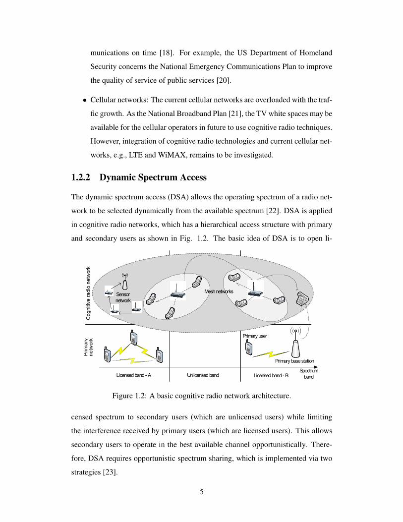
1.2.2 Dynamic Spectrum Access
The dynamic spectrum access (DSA) allows the operating spectrum of a radio net-
work to be selected dynamically from the available spectrum [22]. DSA is applied
in cognitive radio networks, which has a hierarchical access structure with primary
and secondary users as shown in Fig. 1.2. The basic idea of DSA is to open li-
Licensed band - A Licensed band - BUnlicensed band
Primary
network
Cognitive radio network
Spectrum
band
Primary user
Sensor
network
Mesh networks
Primary base station
Figure 1.2: A basic cognitive radio network architecture.
censed spectrum to secondary users (which are unlicensed users) while limiting
the interference received by primary users (which are licensed users). This allows
secondary users to operate in the best available channel opportunistically. There-
fore, DSA requires opportunistic spectrum sharing, which is implemented via two
strategies [23].
5

1. Spectrum overlay does not necessarily impose strict constraints on the trans-
mit power of secondary users, but rather on their transmission time. Conse-
quently, a secondary user accesses a spectrum hole assigned via DSA.
2. Spectrum underlay imposes strict constraints on the transmit power of sec-
ondary users. This power at a certain portion of the spectrum is then low
enough to be regarded as noise by the primary users. Both primary and sec-
ondary users may thus transmit simultaneously in the same channel assigned
via DSA, and this assignment may minimize the mutual interference.
In spectrum overlay cognitive radio, the secondary (cognitive) users are allowed
to opportunistically access spectrum which has already been allocated to primary
users. As this opportunistic access may create interference, secondary users trans-
mit only if primary users are not active. Whenever primary users become active,
secondary users must detect the presence of the primary users reliably, immediately
vacate the channel, and find other free channels for continuing communication. One
of the most important tasks in the spectrum overlay system is thus to identify the
spectrum holes.
1.2.3 Spectrum Sensing
The purpose of spectrum sensing is to identify the spectrum holes for opportunistic
spectrum access. After available channels (spectrum holes) are detected success-
fully, they may be used for communications by a secondary transmitter and a sec-
ondary receiver [24]. Spectrum sensing is performed based on the received signal
from the primary users. Primary users have two states, idle or active. With the pres-
ence of the noise, primary signal detection at a secondary user can be viewed as a bi-
nary hypothesis testing problem in which Hypothesis 0 (H0) and Hypothesis 1 (H1)
are the primary signal absence and the primary signal presence, respectively [25].
Based on the hypothesis testing model, several spectrum sensing techniques have
been developed. They are reviewed next.
6

1.2.4 Spectrum Sensing Techniques
Spectrum sensing techniques include energy detection, matched filter, cyclostation-
ary feature detection, and eigenvalue detection.
• Energy detection: This measures the energy of the received signal within the
pre-defined bandwidth and time period. The measured energy is then com-
pared with a threshold to determine the status (presence/ absence) of the trans-
mitted signal. Not requiring channel gains and other parameter estimates, the
energy detector is a low-cost option. However, it performs poorly under high
noise uncertainty and background interference [26].
• Matched filter: This detector requires perfect knowledge of the transmitted
signal and the channel responses for its coherent processing at the demod-
ulator. The matched filter is the optimal detector of maximizing the signal-
to-noise ratio (SNR) in the presence of additive noise. Since it requires the
perfect knowledge of the channel response, its performance degrades dramat-
ically when there is lack of channel knowledge due to rapid changes of the
channel conditions [27, 28].
• Cyclostationary feature detection: If periodicity properties are introduced in-
tentionally to the modulated signals, the statistical parameters of received sig-
nal such as mean and autocorrelation may vary periodically. Such periodicity
of statistical properties is used in the cyclostationary detection. Cyclosta-
tionary properties of the received signal may be extracted by its input-output
spectral correlation density. The signal absence status can be identified eas-
ily, because the noise signal does not have cyclostationary properties. While
this detector is able to distinguish among the primary user signals, secondary
user signals, or interference. it needs high sampling rate and a large number
of samples, and thus increases computational complexity as well [29–32].
• Eigenvalue detection: The ratio of the maximum (or the average) eigenvalue
to the minimum eigenvalue of the covariance matrix of the received signal
vector is compared with a threshold to detect the absence or the presence of
7

the primary signal. However, if the correlation of the primary signal samples
is zero (e.g., primary signal appears as white noise), eigenvalue detection
may fail - a very rare event. This detector has the advantage of not requiring
the knowledge of the primary signal and the propagation channel conditions.
The main drawback is the computational effort to compute covariance matrix
and eigenvalue decomposition. The threshold selection is challenging as well
[33–35].
1.3 Motivation
The exponential growth of wireless communications has led to spectrum scarcity.
Although cognitive radio has been developed to solve the spectrum scarcity and
spectrum under-utilization issues, many research problems remain open.
Reliable primary user detection via spectrum sensing is one of the critical prob-
lems, and hence spectrum sensing is one of the most challenging and difficult
tasks [36]. Moreover, selecting the best available channel and reducing or elimi-
nating interference to primary users are also essential [37, 38]. All these require-
ments depend on the spectrum sensing technique. Among the spectrum sensing
techniques, energy detection is the most popular one due to its low complexity.
Although energy detection has been well investigated for traditional wireless net-
works, new challenges arise when it is applied in cognitive radio networks.
• A more reliable energy detector (than those in traditional networks) is needed
to minimize interference.
• A much wider spectrum bandwidth needs to be sensed to identify spectrum
holes. Since different spectrum holes experience different signal propagation
conditions, the design and analysis of energy detection is challenging.
• Many transmission environments must be considered. Activities from mul-
tiple licensed wireless applications must be detected. Different applications
may have different population of users, with different mobility patterns, which
have a great impact on the signal reception, and thus, affect energy detection.
8

Thus, to address these research challenges, this thesis focuses on energy detec-
tion for spectrum sensing, and related research problems.
1.4 Problem Statements
Specifically, this thesis addresses five problems, P1-P5, which are related to the
spectrum sensing via energy detection in cognitive radio networks.
P1: Energy detection under channels with both multipath fading and shadowing:
Spectrum holes must be correctly detected by the energy detector, whose per-
formance can be quantified by the false-alarm and detection probabilities.
While the performance of energy detectors on multipath fading has been an-
alyzed extensively, wireless signals also undergo shadowing which severely
impacts the detection capability. Multipath fading superimposed on shad-
owing occurs in practical communication channels. Due to the analytical
intractability of composite fading models, the shadowing effect has been ne-
glected in the literature.
P2: A unified channel model for performance analysis of wireless communica-
tions: Analytical intractability of different propagation models, and the re-
sulting mathematically complicated expressions do not facilitate rapid eval-
uation of energy detection and other wireless network performance. There-
fore, a simple analytical framework is vital, and thus, a unified channel model
which represents typical channel models in various spectrum bands and vari-
ous scenarios is desirable.
P3: A generalized and simplified performance metric for energy detection: The
detection capability of an energy detector depends on many parameters, and is
traditionally characterized through the receiver operating characteristic (ROC)
curve, which is not flexible when more than one parameters change concur-
rently. Further, visual examination of ROC curves to compare different en-
ergy detectors is unreliable. Thus, a generalized and simplified single-valued
9

performance metric, which facilitates energy detector design and analysis, is
desired.
P4: Reliability improvement of energy detector: Spectrum sensing in cognitive
radio may suffer from the notorious hidden terminal problem, which happens
when close by secondary and primary transmitters are blocked by a distur-
bance (e.g., a high building). Although the cooperative spectrum sensing
has been identified as a solution, an extensive performance analysis has been
lacking.
P5: Spectrum sensing in very low SNR: The US FCC and the IEEE 802.22 stan-
dard have determined that cognitive devices must detect with very low false
alarm and missed-detection probabilities within a very short sensing time at
low SNR and low receiver sensitivity. This inherent conflict between low
false alarm and missed-detection probabilities and short sensing time poses
critical challenges to the energy detector design in very low SNR. Little at-
tention was paid to this research problem in the past because of analytical
intractability of traditional frameworks.
1.5 Thesis Outline
Chapters 2–7 provide background knowledge, detailed treatment and new ideas in
order to address the problems P1–P5, which are briefly outlined as follows.
• Chapter 2 contains background knowledge for topics related to this thesis.
The wireless communication channel and its fading are considered through-
out the thesis. The conventional energy detection and its system model are
reviewed to gain further insights of the already existing literature.
• Chapter 3 addresses problem P1, in which the performance of an energy de-
tector for channels with both multipath fading and shadowing is analyzed
by the adoption of the K channel and generalized-K (denoted as KG) chan-
nel. Multipath fading and shadowing effects are shown by using the ROC
curves based on analytical expressions of the average detection probability.
10

The ROC curves are presented for different degrees of multipath fading and
shadowing.
• Composite fading (i.e., multipath fading and shadowing together) has increas-
ingly been analyzed by means of the K channel and related models. Nev-
ertheless, these models do have computational and analytical difficulties as
pointed out in problem P2. Motivated by this context, Chapter 4 proposes a
mixture gamma (MG) distribution for the SNR of mobile radio channels. Not
only is it a more accurate model for composite fading, but is also a versatile
approximation for any fading SNR. With this model, performance metrics
such as the average channel capacity, the outage probability, the symbol error
rate (SER) of general wireless communication networks, and the detection
capability of an energy detector are readily derived. Note that the analysis is
not limited to cognitive radio networks.
• As pointed out in problem P3, a simple figure of merit to describe the per-
formance of an energy detector is desired. Such a measure is the Area Under
the receiver operating characteristic Curve (AUC). In Chapter 5, the AUC is
analyzed for an energy detector with no-diversity reception and with several
popular diversity schemes.
• As a solution to problem P4, a cooperative spectrum sensing cognitive ra-
dio network with much improved reliability is designed based on energy de-
tection, in which multiple cognitive relays in a secondary network can help
forward received primary signals to a fusion center such that detection per-
formance at the fusion center is significantly improved. The detection perfor-
mance of an energy detector used for cooperative spectrum sensing in a cog-
nitive radio network is investigated over channels with both multipath fading
and shadowing in Chapter 6. The analysis focuses on two fusion strategies:
data fusion and decision fusion. The results are extended to multi-hop net-
works as well.
• The IEEE 802.22 WRAN requires spectrum-sensing techniques to identify
11

primary signals with an SNR as low as -20 dB and receiver sensitivity as
low as -116 dBm, which is identified as a challenging problem as in problem
P5. In Chapter 7, under such low-SNR levels, the detection performance of
an energy detector used for spectrum sensing in cognitive radio networks is
investigated, and analytical expressions for performance metrics are derived.
Further, the detection threshold is also optimized to minimize the total error
rate.
∼
12

Chapter 2
Background
This chapter reviews relevant topics for this thesis. For analysis of energy detec-
tion, the wireless channel models which represent small-scale fading, large-scale
fading and composite fading are important. The test statistic of the energy detec-
tor and its distribution depend on the signal model (e.g., Gaussian signal) and the
network (e.g., cooperative networks). Parameters of the energy detector also need
to be carefully designed to achieve target performance metrics. The IEEE 802.22
standard and the cooperative spectrum sensing are also reviewed.
2.1 Mobile Radio Channel
The mobile radio channel refers to the transmission medium between the transmit-
ter and the receiver. Fundamental mobile radio channel propagation effects include
path loss, microscopic (small scale or fast) fading, and macroscopic (large scale or
slow) fading. These effects are modeled as a complex channel gain, h. Additive
thermal noise, with a flat power spectral density, is called the additive white Gaus-
sian noise (AWGN). Including these factors, the received signal may be generically
represented as
y = hs+w (2.1)
where s is the transmitted signal and w is the AWGN term.
The path loss can model the attenuation of signal strength with distance, wave-
length, and antenna heights. In the thesis, while the small-scale fading and the
large-scale fading are considered, the path loss effect is neglected due to analytical
13

difficulties.
2.1.1 Small-Scale Fading and Large-Scale Fading
The small-scale fading, which occurs in indoor environments and also both macro-
cellular and microcellular outdoor environments, results from multipath propaga-
tion due to the reflections and scatters. The constructive and destructive effects of
the multiple signals distort both amplitude and phase of the received signal with
time, which is called the envelope fading, given by Rayleigh, Nakagami-m and Ri-
cian fading models [39]. For Rayleigh fading, the magnitude of the channel gain,
|h|, has Rayleigh distribution given by
f|h|(x) =2x
Ωe−
x2
Ω , 0 ≤ x ≤ ∞ (2.2)
where Ω is the average envelope power. The Nakagami-m fading is a generalized
model for the non-line of sight small-scale fading, which is given as
f|h|(x) =2mmx2m−1
ΩmΓ(m)e−
mx2
Ω , 0 ≤ x ≤ ∞ (2.3)
where 0.5 ≤ m < ∞ is the fading severity parameter, and Γ(·) is the Gamma
function. The Rician channel model fits well with a channel having a dominant
line-of-sight component. If real and imaginary components of h have the mean a
and the variance b, the distribution is given as
f|h|(x) =x
be−
x2+s2
2b I0
(sxb
), 0 ≤ x ≤ ∞ (2.4)
where s =√2a, which is the non-centrality parameter, and I0 (·) is the zeroth-order
modified Bessel function of the first kind.
The large-scale fading, which occurs due to the shadowing effect by buildings,
foliage and other objects, can significantly impact satellite channels, point-to-point
long distance microwave links and macrocellular outdoor communications [40].
The mean-squared amplitude, Ω, represents the shadowing effect which is typically
modeled with the log-normal distribution as [39]
fΩ(x) =ξ
x√
2πσ2ΩdB
e− (10log10(x)−µΩdB)2
2σ2ΩdB , 0 ≤ x ≤ ∞ (2.5)
where ξ = 10ln 10
, and µΩdB and σΩdB are mean and standard deviation of 10log10(Ω),
respectively.
14

2.1.2 Composite Fading
Both microscopic fading and macroscopic fading are modeled by composite shad-
owing/fading distributions. The Rayleigh-lognormal (RL) and Nakagami-lognormal
(NL) are two most common models [39]. But the probability density function (PDF)
of these two composite models are not in closed form, making performance analy-
sis of some applications difficult or intractable. Therefore, the K distribution and
generalized-K orKG distribution have been introduced, by using a gamma distribu-
tion to approximate the lognormal distribution of the shadowing to model channels
with composite multipath fading and shadowing. In [41], the K distribution, a mix-
ture of Rayleigh distribution and gamma distribution, is used to approximate the
Rayleigh-lognormal distribution, referred to as the K channel model, in which the
fading amplitude undergoes multipath fading as a Rayleigh distribution and shad-
owing as a gamma distribution. Therefore, the average power of the fading ampli-
tude, which represents the shadowing effect, follows the gamma distribution. The
PDF of the fading amplitude, denoted as f|h|(x), follows a K distribution which is
given as [42]
f|h|(x) =4
Γ(k)√Ω
(x√Ω
)k
Kk−1
(2√Ωx
), 0 ≤ x ≤ ∞ (2.6)
where Kν(·) is the modified Bessel function of the second kind of order ν, k is the
shaping parameter and Ω represents the mean signal power.
In [43], the KG distribution, a mixture of the Nakagami distribution and gamma
distribution, is presented to approximate the NL distribution, referred to as the KG
channel model. The KG distribution is given as [44]
f|h|(x) =4m
β+12 xβ
Γ(m)Γ(k)Ωβ+12
Kα
[2(mΩ
) 12x
], 0 ≤ x ≤ ∞ (2.7)
where m is the fading parameter, α = k − m, and β = k + m − 1. The KG
distribution reduces to a K distribution when m = 1. Moreover, as m → ∞ and
k → ∞, the KG model tends to a non-fading case, i.e., the AWGN channel. The
accuracy of the approximation is verified by comparison of their moment generating
function (MGF) [42, 44]. The KG model includes special cases, such as the K
15

model, and can also approximate the Nakagami-m model, the RL distribution and
the Suzuki model [41].
Moreover, several other composite models have been developed including the
G- distribution, the Log-normal distribution, and the Gamma distribution [39, 45,
46]. Note that these models are approximations of the RL and NL models.
2.2 System Model of Spectrum Sensing
Primary users are in either idle state or active state. With the presence of the noise,
the signal detection at the receiver can be viewed as a binary hypothesis testing
problem in which Hypothesis 0 (H0) and Hypothesis 1 (H1) are the primary signal
absence and the primary signal presence, respectively [25]. The nth, n = 1, 2, · · · ,
sample of the received signal, y(n), can be given under the binary hypothesis as
[25, 47]:
y(n) =
w(n) : H0
x(n) +w(n) : H1(2.8)
where x = hs.
The complex signal, s has real component sr and imaginary component si, i.e.,
s = sr+jsi.1 The AWGN samples are assumed to be circularly symmetric complex
Gaussian (CSCG) random variables with mean zero (Ew(n) = 0) and variance
2σ2w (Varw(n) = 2σ2
w) where E· and Var· stand for mean and variance,
respectively, i.e., w(n) ∼ CN (0, 2σ2w). A noise sample is denoted as w(n) =
wr(n) + jwi(n) where wr(n) and wi(n) are real-valued Gaussian random variables
with mean zero and variance σ2w, i.e., wr(n), wi(n) ∼ N (0, σ2
w). The channel gain
is denoted as h = hr + jhi. The channel gain can be assumed as a constant within
each spectrum sensing period. In general, (2.8) can be written as
y(n) = θx(n) +w(n) (2.9)
where θ = 0 for H0 and θ = 1 for H1.1A complex number which has real and imaginary components zr and zi, respectively, is denoted asz = zr + jzi.
16

2.3 Spectrum Sensing via Energy Detection
An energy detector is a device that may decide whether the transmitted signal is
absent or present in the noisy environment. Energy detector does not require any
prior knowledge of the transmitted signal (e.g., phase, shape, frequency). The con-
ventional energy detector measures the energy of the received signal over specified
time duration and bandwidth. The energy is then compared with an appropriately
selected threshold to determine the presence or the absence of an unknown signal.
Two models of energy detector can be considered in time-domain implementa-
tions:
1. Analog energy detector which is illustrated in Fig. 2.1(a) is considered in
[48]. It consists of a pre-filter followed by a square-law device and a finite
time integrator. The pre-filter limits the noise bandwidth and normalizes the
noise variance. The output of the integrator is proportional to the energy of
the received signal of the square law device.
2. Digital energy detector is shown in Fig. 2.1(b). It consists of a low pass noise
pre-filter which limits the noise and adjacent signal bandwidths, an analog-to-
digital converter (ADC) which converts continuous signals to discrete digital
signal samples, and a square law device followed by an integrator. The digital
implementation is usually used at the experimental testbed.
( )2
Noise pre-filter Squaring device Integrator
Test
statistics Y(t) ?
( )2
Noise pre-filter Squaring device Integrator
Test
statistics Y(t) ?A/D
ADC
(a)
(b)
Figure 2.1: The conventional energy detectors: (a) analog and (b) digital .
17

The integrator output of any architecture is called decision statistic or test statis-
tic. The test statistic is finally compared at the threshold device followed by deci-
sion device to make the final decision of the presence/absence of transmitted signal.
The test statistic may not always be the integrator output, but it can be any function
which is monotonic with the integrator output [48].
2.4 Test Statistic of Energy Detector
The test statistic of the analog energy detector is given as Λ = 1T
∫ t
t−T[y(t)]2 dt
where T is the time duration [48]. A sample function with bandwidth W and time
duration T can be described approximately by a set of samples N ≈ 2TW . There-
fore, the analog test statistic can be implemented by samples, where the test statistic
is proportional to∑N
n=1 |y(n)|2. In digital implementation, after proper filtering,
sampling, squaring and integration, the test statistic is given by using (2.9) as
Λ =N∑
n=1
|y(n)|2 =N∑
n=1
(er(n)
2 + ei(n)2)
(2.10)
where er(n) = θhrsr(n) − θhisi(n) + wr(n) and ei(n) = θhrsi(n) + θhisr(n) +
wi(n). Since the test statistic only includes the received signal energy, energy detec-
tor is the optimal non-coherent detector for an unknown signal if the signal is Gaus-
sian, uncorrelated and independent with the uncorrelated background noise [49].
The performance of energy detector (or of other detectors) is measured by using
following metrics:
• False alarm probability (Pf ): the probability of deciding the signal is present
while H0 is true, i.e., Pf = P [Λ > λ|H0] where P [·] stands for an event
probability. Pf indicates the probability of undetected spectrum holes. A
large Pf leads to poor spectral efficiency in cognitive radio.
• Missed-detection probability (Pmd): the probability of deciding the signal is
absent while H1 is true, i.e., Pmd = P [Λ < λ|H1], which means a wrong
decision on the unavailable spectrum. A large Pmd means poor reliability,
which introduces unexpected interference to primary users.
18

• Detection probability (Pd): the probability of deciding the signal is present
when H1 is true , i.e., Pd = P [Λ > λ|H1], and thus, Pd = 1− Pmd.
Both reliability and efficiency are expected from the spectrum sensing technique
built into the cognitive radio, i.e., a higher Pd (or lower Pmd) and lower Pf are
preferred.
The statistical properties of Λ are necessary to characterize the performance of
energy detector. Based on the known properties of the received signal and noise, an
accurate and analytically tractable model for Λ is thus vital for further discussion.
While the noise components, wr(n) and wi(n), are zero-mean Gaussian, different
models for the signal to be detected are possible. Therefore, several alternative
models are discussed in the following. The PDFs of Λ under hypotheses H0 and
H1 are denoted as fΛ|H0(x) and fΛ|H1(x), respectively.
2.4.1 Signal Models
Based on the available knowledge of s(n) at receiver, signal can be modeled dif-
ferently, which helps to analyze the distribution of the test statistic under H1. For
example, three different models, S1, S2 and S3, are popularly used in the literature,
and are given as follows.
S1: For given channel gain h, the signal to be detected, y(n), can be assumed
as Gaussian with mean Ey(n) = Ehs(n) +w(n) = hs(n) and vari-
ance Vary(n) = 2σ2w. For the signal transmitted over a flat band-limited
Gaussian noise channel, a basic mathematical model of the test statistic of an
energy detector is given in [48]. The receive SNR can thus be given as
γS1 =|h|2 1
N
∑Nn=1 |s(n)|2
2σ2w
. (2.11)
S2: If the signal sample is considered as random variable which has a Gaussian
distribution, i.e., s(n) ∼ CN (0, 2σ2s), then y(n) ∼ CN (0, 2(σ2
w + σ2s)). The
receive SNR can thus be given as
γS2 =|h|22σ2
s
2σ2w
. (2.12)
19

S3: If the signal sample is considered as random variable with mean zero and
variance 2σ2s , but with an unknown distribution, then y(n) has mean zero and
2(σ2w + σ2
s) variance. The receive SNR can also be given as
γS3 =|h|22σ2
s
2σ2w
. (2.13)
For sufficiently large number of samples, the signal variance can be written by using
its sample variance as 2σ2s ≈ 1
N
∑Nn=1 |s(n)|2 −
(1N
∑Nn=1 s(n)
)2. If the sample
mean goes to zero, i.e., 1N
∑Nn=1 s(n) → 0, 2σ2
s ≈ 1N
∑Nn=1 |s(n)|2, and thus all
the receive SNRs under different signal models which are given in (2.11)-(2.13) are
equal. In general, the instantaneous SNR is denoted as γ.
2.4.2 Distribution of Test Statistics
The exact distributions of the test statistic (2.10) for different signal models are
analyzed in the following under both hypotheses, H0 and H1.
Under H0
In this case, er(n) = wr(n) and ei(n) = wi(n), and er(n) and ei(n) follow
N (0, σ2w). Thus, Λ is a sum of 2N squares of independent N (0, σ2
w) random vari-
ables, and it follows central chi-square distribution which is given as [50]
fΛ|H0(x) =xN−1e
− x
2σ2w
(2σ2w)
N Γ(N), 0 ≤ x <∞. (2.14)
Thus, the false-alarm probability can be derived by using (2.14) as
Pf = P [Λ > λ|H0] =Γ(N, λ
2σ2w)
Γ(N)(2.15)
where Γ(·, ·) is the upper incomplete Gamma function.
Under H1
In this case, the distribution of Λ, fΛ|H1(x), has two different distributions under
two signal models, S1 and S2, for a given channel. However, the distribution of Λ
under S3 cannot be derived.
20

For S1, er(n) and ei(n) follow N (hrsr(n) − hisi(n), σ2w) and N (hrsi(n) +
hisr(n), σ2w), respectively. Since Λ is a sum of 2N squares of independent and non-
identically distributed Gaussian random variables with non-zero mean, Λ follows
non-central chi-square distribution which is given as [50]
fΛ|H1(x) =
(xσ2w
)N−12e− 1
2
(x
σ2w+µ
)
2σ2wµ
N−12
IN−1
(õx
σ2w
), 0 ≤ x <∞, (2.16)
where Iν(·) is the modified Bessel function of the first kind of order ν,
µ =N∑
n=1
(hrsr(n)− hisi(n))2
σ2w
+(hrsi(n) + hisr(n))
2
σ2w
= 2NγS1
which is the non-centrality parameter, and γS1 is given in (2.11). Thus, the detection
probability can be derived for S1 by using (2.16) as
Pd,S1 = P [Λ > λ|H1] = QN
(√2NγS1,
√λ
σw
)(2.17)
where QN(·, ·) is the generalized Marcum-Q function. This signal model is widely
used in the performance analysis of an energy detector in terms of the average
detection probability [51–54].
For S2, er(n) and ei(n) follow N (0, (1 + γS2)σ2w) where γS2 is given in (2.12).
Since Λ is a sum of 2N squares of independent and identically distributed (i.i.d.)
Gaussian random variables with zero mean, Λ follows central chi-square distribu-
tion which is given as
fΛ|H1(x) =xN−1e
− x
2(1+γS2)σ2w
(2(1 + γS2)σ2w)
N Γ(N), , 0 ≤ x <∞. (2.18)
The exact detection probability can be derived for S2 by using (2.18) as
Pd,S2 =Γ(N, λ
2σ2w(1+γS2)
)
Γ(N). (2.19)
This model is used in [55, 56].
For S3, er(n) and ei(n) have unknown distributions, and the exact fΛ|H1(x)
cannot be derived, and it may not be a central or non-central chi-square distribution
as well. However, fΛ|H1(x) can be derived approximately by using the central limit
theorem (CLT).
21

2.4.3 CLT Approach
According to the CLT, the sum of N i.i.d. random variables with finite mean and
variance approaches to a normal distribution when N is large enough. Using the
CLT, the distribution of the test statistic (2.10) can be accurately approximated with
a normal distribution for sufficiently large number of samples as
Λ ∼ N
(N∑
n=1
E|y(n)|2
,
N∑n=1
Var|y(n)|2
).
When the distributions of test statistics under H0 and H1 are Λ ∼ N (m0, σ20) and
Λ ∼ N (m1, σ21), respectively, the performance matrices can be derived as
Pf ≈ Q
(λ−m0
σ0
)and Pd ≈ Q
(λ−m1
σ1
). (2.20)
where Q(·) is the Gaussian-Q function.
If it is possible to evaluate E|y(n)|2 and Var|y(n)|2, the CLT approach can
be applied to H0 and H1 (with any signal model), and the performance matrices can
also be derived as (2.20). The mean and variance for different cases are given as
follows:
E|y(n)|2
=
2σ2
w : H0
2σ2w + |h|2|s(n)|2 : S1
2σ2w + |h|2(2σ2
s) : S2, S3.(2.21)
Var|y(n)|2
=
(2σ2
w)2 : H0
4σ2w(σ
2w + |h|2|s(n)|2) : S1
4(σ2w + |h|2|σ2
s)2 : S2
(2σ2w)
2 + 2|h|2(2σ2w)(2σ
2s) + |h|4(E|s(n)|4] − 4σ4
s) : S3.(2.22)
If s(n) of S3 is complex phase shift keying (PSK) signal, E|s(n)|4 = 4σ4s , and
thus the variance can be evaluated as Var|y(n)|2 = (2σ2w)
2 + 2|h|2(2σ2w)(2σ
2s).
Therefore, the distribution of Λ can be given as
Λ ∼ N
N (N(2σ2
w), N(2σ2w)
2) : H0
N (N(2σ2w)(1 + γ), N(2σ2
w)2(1 + 2γ)) : S1, S3
N (N(2σ2w)(1 + γ), N(2σ2
w)2(1 + γ)2) : S2.
(2.23)
Approximated false-alarm probability and approximated detection probabilities
can be derived by using (2.20) as
Pf ≈ Q
(λ−N(2σ2
w)√N(2σ2
w)
), (2.24)
22

Pd,S1 ≈ Q
(λ−N(2σ2
w)(1 + γ)√N(1 + 2γ)(2σ2
w)
), (2.25)
Pd,S2 ≈ Q
(λ−N(2σ2
w)(1 + γ)√N(1 + γ)(2σ2
w)
). (2.26)
Note that Pd,S3 has the same expression as Pd,S1.
102
10−3
10−2
10−1
100
λ
Pro
babi
lity
ExactCLT
Pf,N=60P
f,N=20
Pd,S1
,N=60
Pd,S2
,N=60P
d,S1,N=20
Pd,S2
,N=20
Figure 2.2: The exact and approximated (CLT) CDFs of the test statistic for S1 andS2 with 2σ2
w = 1 and γ = 5dB.
Fig. 2.2 shows the exact Pf and Pd of the test statistic for S1 and S2.2 Both Pf
and Pd increase significantly when the number of samples increases from N = 20
to N = 60. Fig. 2.2 also shows the CLT approximations of Pf and Pd. The exact
curves (solid-line) match well with the CLT approximations (dashed-line) when
N = 60, while they have a close match when N = 20. This confirms that the test
statistic is approximately Gaussian for a sufficiently large number of samples.
Note that this thesis uses exact Pf and Pd expressions (2.15) (2.17) in Chapters
3–6, and uses approximated Pf and Pd expressions (2.24)-(2.26) (based on CLT) in
Chapter 7.
2Pf and Pd are also the complementary cumulative distribution function (CDF)s of the test statistic.
23
2.5 Design Parameters
The main design parameters of the energy detector are the number of samples and
threshold. However, the performance of the energy detector depends on SNR and
noise variance as well, but the designer has very limited control over them because
these parameters depend on the behavior of the mobile radio channel.
2.5.1 Threshold
A pre-defined threshold λ is required to decide whether the target signal is absent
or present. The threshold determines all performance metrics, Pd, Pf and Pmd,
can vary from 0 to ∞, and selection of its operating threshold is important. The
operating value can be chosen based on the target value of the performance metric
of interest. Although having high Pd while keeping Pf low is preferable (e.g., as
IEEE 802.22 WRAN), these two objectives are conflicting, and may not always be
simultaneously achieved in practice.
When the threshold increases (or decreases), both Pf and Pd are decreased (or
increased). For known N and σw, the common practice of setting the threshold
is based on the constant false alarm probability Pf , e.g., Pf ≤ 0.1. The selected
threshold based on Pf can be given by using (2.24) as
λ∗f =(Q−1(Pf ) +
√N)√
N2σ2w. (2.27)
However this threshold may not guarantee that the energy detector achieves the
target detection probability, e.g., the detection probability should be no less than
0.9 as specified in the IEEE 802.22 WRAN.
2.5.2 Number of Samples
The number of samples is also an important design parameter to achieve the require-
ments on detection and false alarm probabilities. For given false alarm probability
Pf and average detection probability Pd, the minimum required number of samples
can be given as a function of SNR. By eliminating λ from both Pf in (2.24) and Pd
in (2.25) (here signal model S1 is used as an example), N can be given as
N = [Q−1(Pf )−Q−1(Pd)√
2γ + 1]2γ−2 (2.28)
24

which is not a function of the threshold. Due to the monotonically decreasing prop-
erty of Q−1(x), it can be seen that the signal can be detected even in very low SNR
region by increasing N when the noise power is perfectly known. Further, the ap-
proximately required number of samples to achieve a performance target on false
alarm and detection probabilities is in the order of O(γ−2), i.e., energy detector re-
quires more samples at very low SNR [57]. Since N ≈ τfs where τ be the sensing
time and fs be the sampling frequency, the sensing time increases as N increases.
This is a main drawback in spectrum sensing at low SNR because of the limitation
on the maximal allowable sensing time (e.g., the IEEE 802.22 specifies that the
sensing time should be less than 2 seconds).
2.6 IEEE 802.22 Standard
As mentioned in Section 1.2.1, FCC has permitted the TV white space spectrum to
be used by broadband access systems. Several telecommunications standards have
thus been developed to operate in the vacant TV bands based on cognitive radio
technology. Among these standardization efforts [14–16], the IEEE 802.22 WRAN
brings broadband access not only to the WiFi devices but also to general mobile
networks (e.g., micro-, pico- or femto-cells), allowing the use of the cognitive radio
technique on a non-interfering basis [11–13].
The IEEE 802.22 WRAN limits both false alarm (which indicates the level of
undetected spectrum holes) and missed-detection (which indicates the level of unex-
pected interference to primary users) probabilities to 10%. While these two perfor-
mance metrics reflect the overall efficiency and reliability of the cognitive network,
the 10% requirement should be met even under very low SNR conditions, such as
-20 dB SNR with a signal power of -116 dBm and a noise floor of -96 dBm [13].
The IEEE 802.22 WRAN does not prescribe a specific spectrum sensing tech-
nique, and designers are free to select any detection technique such as energy de-
tection, matched filter detection, cyclostationary feature detection, covariance based
detection, etc. [48, 53, 54, 58–65]. While the spectrum sensing techniques perform
well at moderate and high SNRs, in which fine-sensing time can be in order of mil-
25

liseconds (e.g., 25 ms), they perform poorly at a low SNR. Although increasing the
sensing time improves the performance, IEEE 802.22 limits the maximal detection
latency to 2 seconds which may include sensing time and subsequent processing
time. This maximal time limit is critical at low-SNR spectrum sensing.
2.7 Cooperative Spectrum Sensing
Achieving the IEEE 802.22 WRAN spectrum sensing specifications is a tough task
because of shadowing, fading, and time variations of mobile radio channels. More-
over, the hidden terminal problem, which occurs when the link from a primary
transmitter to a secondary user is shadowed (e.g., there is a tall building between
them as shown in Fig. 2.3) while a primary receiver is operating in the vicinity
of the secondary user, presents a tough challenge. Due to this, a secondary user
may fail to notice the presence of the primary transmitter, and then accesses the
licensed channel and causes interference to the primary receiver. To mitigate this
problem, cooperative spectrum sensing has been introduced, in which single coop-
erative node or multiple cooperative nodes are introduced to the secondary network
(Fig. 2.3). Cooperative nodes individually sense the spectrum, and send their col-
lected data to a fusion center. The random spatial distribution of the cooperative
nodes helps to reduce the impact of the hidden terminal problem.
Primary user
Secondary user
(Fusion center)
Building
Cooperative node
Primary network
Secondary
network
Figure 2.3: Cooperative spectrum sensing in a cognitive radio network.
In cooperative spectrum sensing, information from multiple cooperative nodes
is combined at the fusion center to make a decision on the presence or absence
of the primary user. When energy detection is utilized for cooperative spectrum
26

sensing, cooperative nodes report to a fusion center their sensing data, in either
the data fusion or the decision fusion. In data fusion, each cooperative node simply
amplifies the received signal from the primary user and forwards to the fusion center
[66–68]. In decision fusion, each cooperative node makes its own hard decision on
the primary user activity, and the individual decisions are reported to the fusion
center. The performance of such system is analyzed in Chapter 6.
∼
27

Chapter 3
Energy Detection over CompositeFading and Shadowing Channels
This chapter analyzes the performance of an energy detector over mobile radio
channels with composite multipath fading and shadowing effects. These effects
are modeled by using the K and KG channel models. For these channels, the av-
erage detection probabilities of the energy detector are derived for the no-diversity
reception case. A simple approximation of the average detection probability is also
derived for large threshold values. The analysis is then extended to cases with diver-
sity receptions including maximal ratio combining (MRC) and selection combining
(SC).1
3.1 Introduction
The performance of energy detectors has been extensively analyzed by using dif-
ferent channel models assuming a flat, band-limited, Gaussian noise channel [48].
Subsequently, the average detection probability is analyzed over Rayleigh, Rice
and Nakagami fading channels in [69]. Different analytical approaches are given
in [53,70] for the performance of an energy detector with no diversity for Rayleigh,
Rice and Nakagami fading channels and with different diversity receptions such
as MRC, SC and switch-and-stay combining. The performance with equal gain
combining (EGC) under a Nakagami fading channel is analyzed in [54]. All these
1A version of this chapter has been published in IEEE Trans. Wireless Commun., 9: 3662–3670(2010).
28

research papers have focused on multipath fading only.
Shadowing and multipath fading are the two main wireless propagation effects.
While multipath fading can be modeled as a Rayleigh, Rice or Nakagami distri-
bution, shadowing process is typically modeled as a lognormal distribution [39].
Practical communication channels can be modeled as multipath fading superim-
posed on lognormal shadowing, leading to composite channel models. Due to the
analytical intractability of composite fading models, the shadowing effect is some-
times neglected in the literature.
The K and KG channel models described in Section 2.1.2 have been well
adopted for analysis of composite multipath fading and shadowing. Performance of
different wireless communications networks has been analyzed overK orKG chan-
nel model in [42,44,71–73]. The bit error rate (BER) is analyzed for the K channel
model in [71] and for the KG channel model in [73]. The outage probability with
and without co-channel interference is presented based on the KG channel model
in [72]. The average BER with different diversity receptions is derived for the KG
channel model in [44]. Recently, performance of generalized selection combining
receivers over the K channel model is presented in [42]. All these works show the
impact of composite effect (multipath fading and shadowing) in the performance
and design of wireless communications. However, the performance of an energy
detector under composite fading is not available in the literature, and thus it is in-
vestigated in this chapter by using K and KG channel models.
The chapter is organized as follows. The average detection probability of an
energy detector is analyzed without and with diversity techniques in Section 3.2.
Numerical and simulation results are presented in Section 3.3. The concluding
remarks are made in Section 3.4.
3.2 Average Detection Probability
The performance of an energy detector for channels with both multipath fading and
shadowing, by the adoption of the K and KG channel models is analyzed based on
S1 signal model. When the threshold varies from 0 to ∞, the false alarm probability
29
can be easily calculated by using (2.15) for a given number of samples. On the other
hand, the detection probability is determined by threshold, number of samples and
also SNR. Since SNR depends on the channel fading/shadowing, it is essential to
evaluate the average detection probability over the SNR distribution fγ(x) as
Pd =
∞∫0
Pd(x)fγ(x) dx. (3.1)
The critical part of the analysis is the derivation of the average detection proba-
bility. This derivation requires the generalized Marcum-Q function be averaged
over the KG distribution. Since the K and KG channel models contain modified
Bessel functions, the direct integration appears intractable or does not seem to lead
to simple solutions. In order to circumvent these difficulties, the following method
is applied. Since K or KG channel model actually is a result of averaging a con-
ditional Rayleigh or Nakagami PDF by a gamma PDF, the existing results on the
energy detector for Nakagami-m fading case can be averaged over the gamma PDF
(which models the shadowing part) to get the avergae detection probability over
K or KG channel model. This simple trick allows us to avoid the averaging over
the modified Bessel function of the second kind. Similar approach can be applied
for the diversity combining techniques with each diversity branch having identical
instantaneous shadowing effect.
3.2.1 With No-Diversity Reception
The average detection probability of the energy detector can be evaluated by aver-
aging Pd = QN
(√2Nγ,
√λ)
, where σw = 1, in (2.17) over the SNR range, which
can be expressed mathematically as
Pd =
∞∫0
QN(√2Nγ,
√λ)fγ(γ) dγ
=
∞∫0
∞∫0
QN(√
2Nγ,√λ)fγ|Y=y(γ)dγfY (y) dy
=
∞∫0
P Fadd (y)fY (y) dy,
(3.2)
30

where Y is the SNR with only shadowing effect (i.e., multipath fading is excluded),
which follows a gamma distribution [39]
fY (y) =1
Γ(k)Ωkyk−1e−
yΩ , y ≥ 0 (3.3)
and P Fadd (y) =
∫∞0QN(
√2Nγ,
√λ)fγ|Y=y(γ) dγ is the average2 detection prob-
ability with a specific Y value. P Fadd (y) for different applications under different
multipath fading can be expressed using previous results in the literature [53] [69]
[70], by replacing the γ’s in previous results with y. The average detection prob-
ability can be derived after averaging P Fadd (y) by fY (y). This approach appears
mathematically more tractable than the direct integration.
K Channel Model
The average detection probability over the K channel model, PKd , can be evaluated
by replacing each γ of the average detection probability over Rayleigh distribution
in [53, eq. (9)] by y, and averaging over fY (y) as given in Appendix A.1. Thus,
PKd can be expressed as
PKd = e−
λ2
N−2∑n=0
1
n!
(λ
2
)n
+∞∑n=0
(−1)n(λ2
)nΓ(k −N + 1)
n!Γ(k)(NΩ)kU
(k −N + 1; k − n+ 1;
1
NΩ
)
−N−2∑n=0
e−λ2
(λ2
)nΓ(n+ k −N + 1)
n!Γ(k)(NΩ)kU
(n+ k −N + 1; k + 1;
1
NΩ
).
(3.4)
where U(·; ·; ·) is the confluent hypergeometric function of the second kind defined
as [74, eq. (3.383.5)]
∞∫0
e−pxxq−1(1 + ax)−v dx =Γ(q)
aqU(q; q + 1− v;
p
a
)(3.5)
with q > 0, p > 0, a > 0 and v a complex value.
2Here the “average” means the average with respect to multipath fading.
31

KG Channel Model
The average detection probability over KG channel model, PKGd , can be evaluated
by replacing each γ of the average detection probability over Nakagami-m distri-
bution in [53, eq. (7)] by y, and averaging over fY (y) as given in Appendix A.2.
Thus, PKGd can be expressed as
PKGd =
1
Γ(k)
( m
NΩ
)k×
[∞∑s=0
N−1∑n=1
e−λ2
(λ2
)n+s(m)sΓ(s+ k)U
(s+ k; k −m+ 1; m
NΩ
)n!s!(n+ 1)s
+∞∑t=0
m−1∑v=0
(−1)t(λ2)t+vΓ(v + k)
(m−1
m−v−1
)U(v + k; k − t−m+ 2; m
NΩ
)t!v!
+∞∑s=0
m−2∑n=0
n∑a=0
(−1)s(λ2)a+s
(n
n−a
)Γ(a+ k + 1)U
(a+ k + 1; k − s− n+ 1; m
NΩ
)a!s!
](3.6)
where(nk
)is the binomial coefficient defined as
(nk
)= n!
k!(n−k)!, (x)s is the Pochham-
mer symbol defined as (x)s =Γ(x+s)Γ(x)
. This is valid for integer m.
One challenge in calculating the expressions (3.4) and (3.6) is the infinite sums.
As an example, the expression (3.4) is calculated as in the following. The expres-
sion (3.6) can be treated similarly. The expression (3.4) can be rewritten as
PKd = e−
λ2
N−2∑n=0
1
n!
(λ
2
)n
+∞∑n=0
(−1)nan −N−2∑l=0
bl (3.7)
where
an =(λ2)nΓ(k −N + 1)U
(k −N + 1; k − n+ 1; 1
NΩ
)n!Γ(k)(NΩ)k
is the nth term of the auxiliary series∑∞
n=0(−1)nan, and
bl =e−
λ2
(λ2
)lΓ(l + k −N + 1)U
(l + k −N + 1; k + 1; 1
NΩ
)l!Γ(k)(NΩ)k
is the lth term of the finite series∑N−2
l=0 bl. Theoretically, the auxiliary series con-
verges as n → ∞. When λ is small, it is observed that the series converges for
relatively small values of n, and thus, (3.4) can be accurately computed by using
any mathematical software (e.g., MATHEMATICA [75]). When λ is large, the
32

sum requires the evaluation of an for large n, and therefore, accurate computation
of (3.4) is difficult (e.g., numerical underflow and overflow errors degrade the ac-
curacy). For higher λ values, the corresponding values of the average detection
probability as well as the false alarm probability are very small (for instance, it can
be less than 10−3). Thus, an approximation is needed for large λ. Note that the first
and the third terms in (3.7) are finite sums and therefore, can be calculated exactly.
For accuracy of (3.7), it is essential to calculate the second term in (3.7), denoted as
IK =∑∞
n=0(−1)nan, accurately. In the following, convergence acceleration of IK
and an approximation method are given for IK .
Convergence Acceleration
As λ→ ∞, a large number of terms in IK need to be evaluated. This drawback can
be avoided by using a convergence acceleration technique. The idea is to generate
a new sequence by using ak|Nk=0. Consider the partial sums sn =∑n
k=0(−1)kak
for n = 0, 1, . . . , N − 1. The objective is to estimate the limit s∞ by using as few
as possible partial sums. The ϵ-algorithm [76] is a powerful convergence acceler-
ation technique suitable for this purpose. The algorithm generates an array ϵ with
ϵ−1(sn) = 0, ϵ0(sn) = sn, and
ϵr+1(sn) = ϵr−1(sn+1) +1
ϵr(sn+1)− ϵr(sn)(3.8)
where r(≥ 0) is an integer. The acceleration method starts with a partial sum of
IK . It then estimates the converging point of n through (3.8) while keeping adding
adequate terms in IK to reach the required accuracy.
Approximation
After applying binomial expansion with some algebraic manipulations, IK can be
approximated for large λ as
IK ≈ 1
Γ(k)Ωk
N−1∑s=0
(N − 1
s
)N s+1−N
∞∫0
yk−N+se−(λ
2Ny+ y
Ω) dy
=2
Γ(k)(NΩ)k
N−1∑s=0
(N − 1
s
)(λΩ
2N
) p2
Kp
(√2λ
NΩ
) (3.9)
33

where the second equality comes from [74, eq. (3.478.4)] and p = k −N + s+ 1.
The expression (3.9) consists of a finite summation with Kp(·), which is available
in most mathematical software. The accuracy of the average detection probability
depends on the accuracy of this approximation. For instance, a four-decimal-point
accuracy is achieved in the average detection probability when a four-decimal-point
accuracy is achieved in IK .
3.2.2 With Diversity Reception
In this section, the performance of an energy detector is considered with diversity
combining methods. The L diversity branches are independent and modeled with
the K distribution. The same analytical technique can be applied as in (3.2). Two
diversity techniques such as MRC and SC are mainly focused here. Diversity com-
bining techniques are used at the receiver to enhance the receive SNR. However,
they may increase the implementation complexity because receiver may need ad-
ditional knowledge of the network, e.g., knowledge of channel-state information
(CSI).
Maximal Ratio Combining
The MRC is a coherent combining technique which needs CSI in non-coherent
energy detection. Thus, it may increase the design complexity. The MRC receiver
combines all the diversity branches weighted with their corresponding complex fad-
ing gains as shown in Fig. 3.1.
( )2
Transmit
antenna
Receive antennas
Combiner
Square law
device
Energy
detection
1
i
L
Figure 3.1: Energy detection with MRC.
34
The energy detector processes the samples of the combined signal of L diversity
branches, Y(n), which can be given as
Y(n) = Hs(n) +W(n) (3.10)
where H =∑L
l=1 |hl|2 and W(n) =∑L
l=1 h∗lwl(n) are effective channel gain and
noise sample, respectively, and wl(n) and hl are noise and channel coefficient of
the lth branch, respectively. The output signal of the MRC can be written as (3.10).
Thus the test statistic is given as
Λ =N∑
n=1
|Y(n)|2 . (3.11)
The effective number of samples for the test statistic is N . The instantaneous SNR
of the combiner output is thus γMRC = γ1 + γ2 + ... + γL. Since energy detector
compares the received energy after the L i.i.d. branches are combined, the expres-
sion of the false-alarm probability is same as (2.15) and the instantaneous detection
probability for AWGN channels can be given as Pd = QN
(√2NγMRC,
√λ)
. To
derive the average detection probability, Pd should then be averaged over the Ray-
leigh fading first, and then averaged over the shadowing. The PDF of γMRC for i.i.d.
Rayleigh fading channels is given by [39]
fγMRC(x) =xL−1 e−
xγ
Γ(L)γL(3.12)
where γ is the average SNR in any branch (note that the “averaging” is on fading
only, excluding shadowing). The fγMRC(x) in (3.12) is similar to the PDF of γ under
Nakagami fading in no-diversity. Therefore, after averaging on Rayleigh fading,
the Pd under MRC (PMRCd ) can be obtained from the average detection probability
for a Nakagami channel with no diversity (i.e. by replacing m by L and y by Ly
in (A.1) in the Appendix). Therefore, the overall average detection probability for
the K channel model with MRC, PMRCd , can be obtained by averaging the “average
detection probability for a Nakagami channel with no diversity” over a gamma dis-
tribution, which is exactly the expression PKGd in (3.6), but with m replaced by L
and Ω replaced by LΩ.
35

Selection Combining
The combiner selects the branch having the strongest SNR among all diversity
branches. The SNR at the output of the combiner is γSC = maxγ1, γ2, ..., γL.
The PDF of γSC, without shadowing, is given in [70, eq. (29)]. Replacing each γ
in [70, eq. (30)] by y and averaging it over fY (y), the average detection probability
for SC diversity scheme under the K channel model, P SCd , can be evaluated as
P SCd = L
L−1∑p=0
(−1)p
p+ 1
(L− 1
p
)PKd
(Ω
p+ 1
)where PK
d
(Ω
p+1
)is the PK
d in (3.4) with the replacement of each Ω by(
Ωp+1
).
3.3 Numerical and Simulation ResultsValidation of the Analysis
Analytical results in (3.4) and (3.6) are verified by numerical methods3 through the
Gaussian-Legendre method and Monte Carlo simulations, as shown in Fig. 3.2a.
The expressions (3.4) and (3.6) are calculated by MATHEMATICA software
package [75], as shown in Fig. 3.2a by legend “Equation (3.4)” and “Equation
(3.6)”. Since the number of terms to sum up to achieve the required accuracy (e.g.,
up to four decimal points) increases with the increase of λ, an acceleration method
is used, in which an ϵ-algorithm [76] is applied to calculate the alternative series
in (3.4) and (3.6). As an example, the converging points of n (which reaches the
required accuracy) for different λ values are given in Table 3.1, for the equation
(3.4), the ϵ-algorithm, and the Gaussian-Legendre method used in the numerical
approximations.
Numerical integration is performed with the Gaussian-Legendre method, which
is explained here briefly. If an integral is in the form∫ 1
−1f(x) dx, the Gaussian-
Legendre rule can be applied as1∫
−1
f(x) dx ≈n∑
i=1
wif(xi)
3Note that the numerical methods are only for numerical calculation of the expression (3.4) and(3.6). On the other hand, the expression (3.9) is an approximation for (3.4).
36

0 20 40 60 80 1000
0.2
0.4
0.6
0.8
1
λ
Pd
Equation (3.4): m=1Equation (3.6): m=2Equation (3.6): m=3Gaussian−Legendre: m=1Gaussian−Legendre: m=2Gaussian−Legendre: m=3Simulation: m=1Simulation: m=2Simulation: m=3
(a)
40 80 1200
0.04
0.08
0.12
λ
I K
Exact I
K
Approximated IK in equation (3.9)
(b)
Figure 3.2: (a) Comparison of analytical expressions (3.4) and (3.6) with numericalapproximations by the Gaussian-Legendre method, and Monte Carlo simulations(N = 2, k = 5.5 and γ = 10 dB); (b) Comparison of exact IK with approximationin (3.9).
Converging point of (n)λ = 25 λ = 50 λ = 75 λ = 100
Equation (3.4) 20 50 84 114ϵ−Algorithm 11 15 19 23
Gaussian-Legendre 38 38 38 38
Table 3.1: Number of terms required to get the accuracy up to four decimal points.
by a suitable choice of the nodes (Legendre points) xi’s and weights wi’s (i =
1, ..., n), where n is the number of nodes. The integral of IK in the form of∫∞0h(y) dy can be transformed to the form
∫ π2
0ϕ(θ) dθ by using the substitution
y = tan θ. Further, it can be transformed to the form∫ 1
−1f(x) dx using the sub-
stitution θ = π4x + π
4. With the help of the three-term recurrence relation, nodes
xi and weights wi can be computed from the associated eigenvalues and eigenvec-
tors [77, Table 25.4]. Therefore, the Gaussian-Legendre method is suitable for IK
to evaluate (3.4) numerically. A similar method can be applied to evaluate (3.6).
Fig. 3.2a shows that the analytical results in (3.4) and (3.6) match well with the
simulations, and the Gaussian-Legendre method provides an accurate approxima-
tion.
37

Accuracy of the Approximation for IK
In Fig. 3.2b, IK (exact and approximation) vs λ is plotted. The approximation acts
as a lower bound for all λ’s and the bound gets tighter when λ increases from 0
to ∞ (i.e., for large λ’s). As an example, accuracy of four decimal points can be
achieved when λ > 140 with N = 3, k = 5.5 and Ω = 1. However, it should
be noted that for small λ’s (practical threshold range), (3.4) and (3.6) can be used
directly to evaluate the accurate detection probabilities without approximation. The
approximation helps for asymptotic analysis.
0 0.2 0.4 0.6 0.8 10
0.1
0.2
0.3
0.4
0.5
0.6
0.7
0.8
0.9
1
Pf
Pd
k = 0.5k = 1k = 20
5 dB
15 dB
0 dB
(a)
0 0.2 0.4 0.6 0.8 10
0.1
0.2
0.3
0.4
0.5
0.6
0.7
0.8
0.9
1
Pf
Pd
m = 1m = 2m = 4m = 7
5 dB
10 dB
(b)
Figure 3.3: (a) ROC curves for the K channel model with different k (N = 1,γ = 0, 5, 15 dB); (b) ROC curves for KG channel model with different fadingparameters, m (k = 5.5, N = 1, γ = 5, 10 dB).
Impact of the Shadowing and Fading
Fig. 3.3a shows the ROC curves (which are illustrated by Pd vs Pf [78]) for the
K channel model with different k and average SNR γ. With the increase of k, an
improvement in the detection probability is observed. This is because increasing k
diminishes the shadowing effect. When k → ∞, the channel is a Rayleigh fading
model. ForKG channel, Fig. 3.3b shows effect of multipath fading with fixed shad-
owing (k = 5.5). Differentm values are taken, with γ = 5, 10 dB. For largerm, the
receiver has a higher detection probability with a lower false alarm probability, i.e.,
38

the channel fading conditions improve with the reduced fluctuations of the signal
strength.
0 0.2 0.4 0.6 0.8 10.1
0.2
0.3
0.4
0.5
0.6
0.7
0.8
0.9
1
Pf
Pd
No diversityMRC L = 2SC L = 2MRC L = 3SC L = 3
Figure 3.4: ROC curves for L-branch MRC and SC diversity receptions with Kchannel model (N = 3, k = 6, γ = 5 dB).
Performance of Diversity Receptions
The performance of MRC and SC diversity schemes with different number L of
diversity branches, which have the same instantaneous shadowing, is illustrated
in Fig. 3.4. There is an obvious diversity gain in the case of diversity systems
compared to no-diversity system (the case with L = 1). Further, MRC always
outperforms SC.
Shadowing Effect
Further, it is important to notice the differences between Rayleigh-lognormal dis-
tribution and K distribution. In general, the performance of shadowing effect is
compared with respect to shadow standard deviation σΩ and mean µΩ in lognor-
mal distribution [39, eq. (2.200)]. The relationships between the parameters in
Rayleigh-lognormal distribution (σΩ and µΩ) and parameters in K distribution (k
39

0 0.2 0.4 0.6 0.8 10
0.1
0.2
0.3
0.4
0.5
0.6
0.7
0.8
0.9
1
Pf
Pd
k = 1.35k = 0.63k = 0.35σΩ = 4.5 dB
σΩ = 8 dB
σΩ = 13 dB
Figure 3.5: Comparison of K channel model with Rayleigh-lognormal channel.
and Ω) can be obtained as [41]
ξµΩ = lnΩ + Ψ(k) and (ξσΩ)2 = Ψ
′(k)
where ξ = ln 1010
, Ψ(·) is the psi function [77], and Ψ′(·) is the first derivative of
Ψ(·). Fig. 3.5 shows the ROC curves of the energy detector for σΩ ≈ 4.5 dB, 8 dB
and 13 dB to represent urban area, typical microcell and worst case of macrocell,
respectively. The respective k and µΩ values for σΩ ≈ 4.5, 8.0, 13 dB are k ≈
1.35, 0.63, 0.35 and µΩ ≈ 2.5155, -3.2254, -9.893 dBm with Ω =2, respectively.
Fig. 3.5 shows that the K distribution is a well-approximated model for the the
Rayleigh-lognormal distribution.
3.4 Conclusion
The performance of an energy detector under both multipath fading and shadowing
effects is studied by using K and KG channel models. The average detection prob-
abilities are derived along with the approximations for large λ values. Convergence
acceleration based on the ϵ-algorithm is suggested to efficiently compute the infi-
nite series representation. Moreover, the numerically efficient Gaussian-Legendre
40

quadrature is useful for numerical approximations. These results show that the de-
tection probability increases with the fading parameterm and shadowing parameter
k. The reason is that as m → ∞ and k → ∞, the channel approaches the AWGN
channel. Furthermore, when diversity receptions such as MRC and SC are used to
boost the performance of the energy detector, their performance is also analyzed
under multipath faded and shadowed diversity branches. The ROC reveals the ef-
fect of diversity advantage, and, as expected, MRC improves the performance of
the energy detector more than SC.
∼
41

Chapter 4
A Mixture Gamma Distribution toModel the SNR of Wireless Channels
As discussed in Section 2.1.2, composite fading which includes multipath fading
and shadowing has increasingly been analyzed by means of the K channel and
related models. Nevertheless, these models do have computational and analytical
difficulties when energy detection and other wireless network performance are an-
alyzed. Motivated by this problem, this chapter develops a mixture gamma (MG)
distribution which can represent several common wireless channels. The accuracy
of the MG representation of composite fading channels and small-scale fading chan-
nels is also examined. Performance analysis and numerical results are given from
the unified analytical framework.1
4.1 Introduction
Performance Analysis Based on K and KG Models
The use of K and KG models for performance analysis has greatly increased re-
cently (see [44,73,79–86], among many others). For instance, the statistics of SNR,
the average channel capacity and the BER are analyzed in [73,79]. The outage per-
formance, the average BER, and the channel capacity of several adaptive schemes
are derived in [80]. The average output SNR, amount of fading and outage prob-
ability of different diversity receivers are derived in [44]. The closed-form BER
1A version of this chapter has been published in IEEE Trans. Wireless Commun., 10: 4193–4203(2011).
42
is derived for (post-detection) EGC in [81]. The performance of dual-hop non-
regenerative relays and multihop regenerative relays is analyzed in [82–84]. The
average BER of orthogonal frequency division multiplexing (OFDM) systems is
evaluated in [85]. The ergodic capacity of multiple-input multiple-output (MIMO)
systems is investigated in [86]. The performance of an energy detector is analyzed
in Chapter 3 of this thesis. These studies and others show the importance of K and
KG models.
Limitations of K and KG Models
While Rayleigh-lognormal (RL) and Nakagami-lognormal (NL) do not have closed-
form PDFs, the K, KG and G- models do. Nevertheless, their PDFs include special
functions (e.g., modified Bessel functions). Consequently, mathematical complica-
tions arise in the evaluation of wireless performance metrics. For instance, the CDF
of the KG model is derived in [73] by using generalized hypergeometric functions.
The computation of such functions can be difficult as their series expressions may
give rise to numerical issues. Asymptotic expansions may hence be required for
certain ranges of the parameters and the variables. Moreover, the PDF of a sum of
SNRs (required in MRC) is intractable. As well, even numerical methods for MRC
by using the characteristic function approach is quite difficult due to the Whittaker
function [46]. To avoid these difficulties, a KG random variable (RV) is approxi-
mated by a Gamma RV in [46], and the PDF of the sum of independent KG RVs
is further approximated by PDF of another KG RV [87]. These approximations use
moment matching.
While performance evaluation over composite channels is highly important, the
use ofK,KG and G models has analytical and/or computational difficulties. Hence,
an alternative approach is developed by using the MG distribution in this chapter.
The rest of the chapter is organized as follows. The MG distribution is described
in Section 4.2. Several common mobile radio channels are represented by using the
MG model in Section 4.3. In Section 4.4, the accuracy of the MG representation
of composite fading channels and small-scale fading channels is examined. Perfor-
mance analysis and the numerical results from the unified framework are shown in
43

Section 4.5 and Section 4.6. The concluding remarks are in Section 4.7.
4.2 Mixture Gamma Distribution
The MG distribution provides several advantages due to several reasons. First, since
it is a linearly weighted sum of gamma distributions, it inherits several advantages
of the gamma distribution. For example, the MGF and CDF, which are required
in wireless system analysis, have mathematically tractable expressions. Second,
this distribution can approximate not only composite fading channels, but also any
small-scale fading channels. Third, high accuracy is possible by adjusting the pa-
rameters. Overall, by using the MG model, performance of any wireless systems
over a variety of fading channels can be analyzed in a unified framework.
In [88], it is shown that any function f(x), where limx→+∞
f(x) → 0 and x ∈
(0,∞), can be given as f(x) = limu→+∞
Fu(x) where Fu(x) := e−ux∑∞
k=0(ux)k
k!f(ku
),
u > 0. Thus, an arbitrarily close approximation to f(x) can be obtained by increas-
ing the number of terms in the mixture [89]. Note that Fu(x) is a weighted sum
of gamma PDFs. This result provides the motivation for using the MG distribution
to represent any wireless SNR models. We start with the SNR distribution, which
is required for analysis of wireless communication systems. The instantaneous re-
ceived SNR and the average SNR are denoted by γ and γ, respectively.
Probability Density Function (PDF)
The following MG distribution is proposed to approximate the PDF of γ as
fγ(x) =S∑
i=1
wifi(x) =S∑
i=1
αixβi−1e−ζix, x ≥ 0 (4.1)
where fi(x) =ζβii xβi−1e−ζix
Γ(βi)is a standard Gamma distribution, wi =
αiΓ(βi)
ζβii
, S is
the number of terms, and αi, βi and ζi are the parameters of the ith, i = 1, · · · , S,
Gamma component. Further,∑S
i=1wi = 1 as∫∞0fγ(x) dx = 1. The special
case S = 1 reverts to SNR distributions of Rayleigh and Nakagami-m fadings.
Discussion of how to choose S is provided in Section 4.4. Note that formula (4.1)
can approximate the PDF of any positive random variable.
44

Cumulative Distribution Function (CDF)
The CDF of the MG distribution can be evaluated as Fγ(x) =∫ x
0fγ(t) dt to yield
Fγ(x) =S∑
i=1
αiζ−βi
i γ (βi, ζix) (4.2)
where γ(·, ·) is the lower incomplete gamma function [74, eq. (8.350.1)].
Moment Generating Function (MGF)
The MGF of MG distribution, Mγ(s), can be evaluated as Mγ(s) = Ee−sx.
Thus, Mγ(s) =∫∞0e−sxfγ(x) dx can be derived as
Mγ(s) =S∑
i=1
αiΓ(βi)
(s+ ζi)βi. (4.3)
Moments
The r-th (r = 0, 1, · · · ,∞) moment associated with the MG distribution, mγ(r),
can be calculated as mγ(r) = Eγr, to yield
mγ(r) =S∑
i=1
αiΓ(βi + r)ζ−(βi+r)i . (4.4)
The mathematically tractable expressions (4.1)-(4.4) demonstrate the major ben-
efit of the MG distribution. These performance metrics have convenient expressions
without complicated special functions. This fact can facilitate the performance stud-
ies enormously. If a given mobile radio channel can be represented as an MG dis-
tribution, the common performance metrics such as error rates, outage and others
are immediately derived, with details given in Section 4.5.
4.3 MG Distribution for Typical mobile radio chan-nels
This section shows how to represent the SNR PDF of the NL, K, KG, κ-µ, Hoyt,
η-µ and Rician channel models in the form of an MG model, as in (4.1).
45

4.3.1 Nakagami-lognormal Channel
The SNR distribution of the NL channel is a gamma-lognormal (GL) distribution,
given as [90]
fγ(x) =
∞∫0
xm−1e−mxρy
Γ(m)
(m
ρy
)me−
(ln y−µ)2
2λ2
√2πλy
dy (4.5)
where m is the fading parameter in Nakagami-m fading, ρ is the unfaded SNR,
and µ and λ are the mean and the standard deviation of the lognormal distribution,
respectively. When m = 1, expression (4.5) is the SNR distribution of the RL
distribution. The fading and shadowing effects diminish for larger m and smaller
λ, respectively. A closed-form expression of the composite GL SNR distribution is
not available in the literature.
By using substitution t = ln y−µ√2λ
, expression (4.5) can be written as
fγ(x) =xm−1
√π Γ(m)
(m
ρ
)m∞∫
−∞
e−t2g(t) dt (4.6)
where g(t) = e−m(√2λt+µ)e−
mρe−(
√2λt+µ)x. The integration, I =
∫∞−∞ e−t2g(t) dt,
in (4.6) is a Gaussian-Hermite integration which can be approximated as I ≈∑Si=1wig(ti) where ti and wi are the abscissas and weight factors for the Gaussian-
Hermite integration [77]. Therefore, fγ(x) in (4.6) can be expressed as the MG dis-
tribution given in (4.1). After normalization of∫∞0fγ(x) dx = 1, parameters can
be given as
αi = ψ(θi, βi, ζi), βi = m, ζi =m
ρe−(
√2λti+µ), θi =
(m
ρ
)mwie
−m(√2λti+µ)
√πΓ(m)
(4.7)
where ψ(θi, βi, ζi) = θi∑Si=1 θiΓ(βi)ζ
−βii
. Function ψ(θi, βi, ζi) is also used for subse-
quent cases.
4.3.2 K and KG Channels
The SNR distribution of theKG channel has a closed-form expression with the nth-
order modified Bessel function of the second kind [73]. With some mathematical
46

simplifications, the SNR distribution of the KG channel, which is a gamma-gamma
distribution, can be rewritten in an integral form as
fγ(x) =λmxm−1
Γ(m)Γ(k)
∞∫0
e−tg(t) dt (4.8)
where g(t) = tα−1e−λxt , λ = km
γand α = k−m. Here k and m are the distribution
shaping parameters, which represent the multipath fading and shadowing effects of
the mobile radio channel, respectively. The integral in (4.8), I =∫∞0e−tg(t) dt,
can be approximated as a Gaussian-Laguerre quadrature sum as I ≈∑S
i=1wig(ti)
where ti and wi are the abscissas and weight factors for the Gaussian- Laguerre
integration [77]. Thus, (4.8) can be written as the MG distribution with parameters
αi = ψ(θi, βi, ζi), βi = m, ζi =λ
ti, θi =
λmwitα−1i
Γ(m)Γ(k)(4.9)
for i = 1, · · · , S.
4.3.3 η-µ Channel
The η-µ channel model is a generalized form to model the non-line of sight small-
scale fading of a mobile radio channel [91]. The Rayleigh, Nakagami-m and Hoyt
distributions are special cases of the η-µ channel model. The η-µ SNR distribution
is given as [92]
fγ(x) =2√πµµ+ 1
2hµxµ−12 e
−2µhxγ
Γ(µ)Hµ− 12 γµ+
12
Iµ− 12
(2µHx
γ
)(4.10)
where the parameter µ =(1+H2/h2)Eγ2
2Varγ (µ > 0) represents the number of multi-
path clusters, and Iv(·) is the vth-order modified Bessel function of the first kind.
Parameters h and H are to be explained in the following. The η-µ channel includes
two fading formats, Format 1 and Format 2, for two different physical represen-
tations. In Format 1, the independent in-phase and quadrature components of the
fading signal have different powers, and η (0 < η < ∞) is the power ratio of the
in-phase component to the quadrature component. Two parameters h and H are
defined as h = 2+η−1+η4
and H = η−1−η4
, respectively. In Format 2, the in-phase
47
and quadrature components of the fading signal are correlated and have identical
powers. η (−1 < η < 1) is the correlation coefficient between the in-phase and
quadrature components. Two parameters h and H are defined as h = 11−η2
and
H = η1−η2
, respectively [91].
Only a few performance studies for the η-µ channel have been published in
the literature, probably because the modified Bessel function of the first kind in
(4.10) leads to mathematical complexity [92–95]. In the following, the η-µ SNR
distribution is approximated by using the MG distribution.
For a real number v, the function Iv(z) can be computed using [74]
Iv(z) =∞∑k=0
1
k!Γ(v + k + 1)
(z2
)2k+v
. (4.11)
Therefore, the η-µ SNR distribution (4.10) can be given in an alternative form as
fγ(x) =2√πµµ+ 1
2hµe−2µhx
γ
Γ(µ)Hµ− 12 γµ+
12
∞∑i=1
(µHγ
)2i+µ− 52x2µ−3+2i
(i− 1)!Γ(µ+ i− 12). (4.12)
The required accuracy2 to approximate the exact fγ(x) can be achieved by summing
a finite number, S, of terms in (4.12). By matching the two PDFs given in (4.10)
and (4.12), the parameters of the MG distribution can be evaluated as
αi =ψ(θi, βi, ζi), βi = 2(µ− 1 + i), ζi =2µh
γ,
θi =2√πµµ+ 1
2hµ
Γ(µ)Hµ− 12 γµ+
12
(µHγ
)2i+µ− 52
(i− 1)!Γ(µ+ i− 12).
(4.13)
Alternatively, the vth-order modified Bessel function of the first kind, Iv(z), can be
approximated by using the integral representation [74, eq. (8.431.5)]
Iv(z) =
π∫0
ez cosϑ cos(vϑ) dϑ
π−
∞∫0
sin(vπ)e−z cosh t−vt dt
π. (4.14)
With ϑ = uπ2+ π
2and vt = p, Iv(z) can be further written as Iv(z) = I1− I2, where
I1 =∫ 1
−1g1(u) du is a Gaussian-Legendre integration, and I2 =
∫∞0e−pg2(p) dp
2The required accuracy can be defined in terms of the mean square error (MSE) between the exactand approximated expressions or by matching the first r moments.
48

is a Gaussian-Laguerre integration where g1(u) = 12e−z sin(πu
2) cos
((u+ 1)πv
2
)and
g2(p) = sin(πv)e−z cosh( pv)/(πv). Similar to Section 4.3.1 with Gaussian-Hermite
integration, the SNR distribution of the η-µ channel can be approximated by the
MG model.
4.3.4 Nakagami-q (Hoyt) Channel
Satellite links with strong ionospheric scintillation can be modeled with this distri-
bution, and its SNR distribution is given as [90]
fγ(x) =1 + q2
2qγe− (1+q2)2
4q2γxI0
(1− q4
4q2γx
)(4.15)
where I0(·) is the zeroth-order modified Bessel function of the first kind. The fading
parameter q varies from 0 to 1, where q = 0 and q = 1 represent the one-sided
Gaussian and Rayleigh distributions, respectively. Further, this distribution is a
special case of the η-µ distribution when µ = 12
and η = q2. Using Format 1 of the
η-µ distribution, the parameters of the MG distribution for the Nakagami-q channel
can be derived from (4.13) to yield
αi = ψ(θi, βi, ζi), βi = 2i− 1, ζi =(1 + q2)2
4q2γ, θi =
(1 + q2)(
1−q4
8q2γ
)2i−2
2qγΓ(i)(i− 1)!.
(4.16)
4.3.5 κ-µ Channel
The κ-µ distribution fits well with line-of-sight channels. Nakagami-n (Rician)
and Nakagami-m channels are special cases of the κ-µ channel. The κ-µ SNR
distribution is [92]
fγ(x) =µ(1 + κ)
µ+12
κµ−12 eµκγ
µ+12
xµ−12 e−
µ(1+κ)γ
xIµ−1
(2µ
√κ(1 + κ)
γx
)(4.17)
where κ (κ > 0) is the power ratio of the dominant components to the scattered
components of the signal, and µ (µ > 0) is defined as µ = (1+2κ)Eγ2(1+κ)2Varγ . Since fγ(x)
includes the modified Bessel function of the first kind with the square root of the
random parameter x, it is difficult to obtain the MG form with one of the Gaussian
49
integration methods, as discussed in previous subsections. To address this difficulty,
the κ-µ SNR distribution given in (4.17) can be written using (4.11) as
fγ(x) =µ(1 + κ)
µ+12
κµ−12 eµκγ
µ+12
∞∑i=1
[µ2i+µ−3(
κ(1+κ)γ
) 2i+µ−32
Γ(µ− 1 + i)(i− 1)!xµ+i−2e−
µ(1+κ)γ
x
]. (4.18)
The required accuracy for approximating the exact fγ(x) can be achieved by sum-
ming a finite number, S, of terms in (4.18). By matching the two PDFs given in
(4.17) and (4.18), the parameters of the MG distribution can be evaluated as
αi =ψ(θi, βi, ζi), βi = µ+ i− 1, ζi =µ(1 + κ)
γ,
θi =µ(1 + κ)
µ+12
κµ−12 eµκγ
µ+12
µ2i+µ−3(
κ(1+κ)γ
) 2i+µ−32
Γ(µ− 1 + i)(i− 1)!.
(4.19)
Alternatively, one can use a different approach in which the MGF of SNR under
κ−µ distribution can be matched with the MGF of SNR under the MG distribution
given in (4.3). Using the power series expansion of the exponential function ex =∑∞n=0
xn
n!, the MGF of the κ-µ SNR distribution given in [93] can be re-written as an
infinite form. By matching the two MGFs, the parameters of (4.1) can be evaluated.
4.3.6 Nakagami-n (Rician) Channel
The Nakagami-n or Rician channel model fits well with channels having a strong
line-of-sight component. The corresponding SNR distribution is given as [90]
fγ(x) =(1 + n2)e−n2
γe−
(1+n2)γ
xI0
(2n
√(1 + n2)
γx
)(4.20)
where n is the fading parameter (0 ≤ n < ∞), and the Rician factor K is given
as K = n2. The Nakagami-n distribution is a special case of the κ-µ distribution
when µ = 1 and κ = n2. Therefore, the parameters of the MG distribution given in
(4.1) can be evaluated as
αi = ψ(θi, βi, ζi), βi = i, ζi =(1 + n2)
γ, θi =
(1 + n2)
en2 [(i− 1)!]2γ
(n2(1 + n2)
γ
)i−1
.
(4.21)
50

4.3.7 Rayleigh and Nakagami-m Channels
The SNR distributions of the Rayleigh and Nakagami-m channels are exponential
and gamma distributions, respectively [90, eq. (2.7) and (2.21)]. The two distribu-
tions are special cases of the MG distribution. When the Rayleigh distribution is
written in the MG form given in (4.1), the corresponding parameters are S = 1,
α1 = 1γ
, β1 = 1 and ζ1 = 1γ
. For the Nakagami-m distribution, the corresponding
parameters are S = 1, α1 =mm
Γ(m)γm , β1 = m and ζ1 = mγ
.
4.4 Determination of the Number S
For the MG distribution, the number of components S needs to be determined. This
can be selected as the minimum value such that (i) the MSE or Kullback-Leibler
(KL) divergence between the target distribution and the MG distribution is below a
threshold; or (ii) the first r moments of the two distributions match.
2 4 6 8 10
10−4
10−3
10−2
10−1
S
MS
E
KG
GGammaLog−normalMG
(a)
2 4 6 8 1010
−4
10−3
10−2
10−1
100
S
KL
dive
rgen
ce
KG
GGammaLog−normalMG
(b)
Figure 4.1: (a) The MSE versus S when the GL distribution is approximated byKG, G, Gamma, Log-normal and MG for m = 2.7, λ = 1, µ = 0, and the averageSNR = 0 dB; (b) The KL divergence (DKL) versus S when the GL distribution isapproximated by KG, G, Gamma, Log-normal and MG for m = 2.7, λ = 1, µ = 0,and the average SNR = 0 dB.
51

4.4.1 Accuracy of MG Distribution to Approximate mobile ra-dio channel SNR
In the literature, the composite GL model has been approximated by KG [43],
G [45], Log-normal [39], and Gamma models [46]. Here, the accuracy of the MG
approximation is compared with that of those approximations. One of the pos-
sible measures of accuracy is the MSE between two PDFs: the approximate PDF,
fApp(x), and the exact PDF, fExt(x), where MSE = E(fExt(x)− fApp(x))
2. An-
other possible measure of accuracy is the KL divergence (DKL) between fApp(x)
and fExt(x), where DKL =∫∞−∞ fExt(x)log fExt(x)
fApp(x)dx.3
The KG, G, Log-normal and Gamma distributions are selected for the compar-
ison. The Log-normal approximation and the Gamma approximation are obtained
by approximating GL PDF by a Log-normal PDF [39], and KG PDF by a Gamma
PDF [46], respectively. The MSEs and DKLs between the GL and its MG approx-
imation (eq. (4.7)), GL and KG, GL and G, GL and Log-normal, and GL and
Gamma can be calculated numerically, as shown in Fig. 4.1a and Fig. 4.1b, respec-
tively, for m = 2.7, λ = 1, µ = 0, and the average SNR = 0 dB. The parameters
of KG, G, Log-normal and Gamma distributions to match the target GL distribu-
tion are obtained from [39, 41, 45, 46]. The MSE and DKL between GL and MG
distributions are less than 10−3 when the number of components S ≥ 6 and S ≥ 8,
respectively. Based on MSE, MG model is better than Gamma, Log-normal, KG
and G models when S ≥ 2, 2, 4 and 5, respectively. Based on KL divergence, MG
model is better than Gamma, Log-normal, KG and G models when S ≥ 3, 3, 4 and
6, respectively. It can be seen that MSE and KL divergence give similar results for
the minimum value of S that makes the MG model more accurate than Gamma,
Log-normal, KG or G model. Further, these MSE and DKL with MG model de-
crease significantly as S slightly increases.
This fact is also evidenced by Fig. 4.2a, which shows the CDFs of the GL
and its approximations by KG, G, Log-normal, Gamma and MG models. These
curves are plotted on a GL paper. The ordinate of the GL paper is obtained using3Although both the MSE and the KL divergence are measures of the difference between two PDFs,they give different measurements. Nevertheless, they give similar results for the minimum value ofS that makes the MG model more accurate than Gamma, KG or G model, as shown subsequently.
52

10−4
10−2
100
1e−6
1e−5
1e−4
0.001
0.01
0.10.20.30.40.50.60.70.80.9
0.99
0.999
1−(1e−4)
x
CD
F
GLK
G
GGammaLog−normalMG
(a)
0 2 4 6 8 100
0.1
0.2
0.3
x
f γ(x)
K
G (m = 2, k = 3, S = 15)
Hoyt (q2 = 0.5, S = 3)η−µ (η = 3.5, µ = 10, S = 8)
Rician (n2=3, S = 16)κ−µ (κ = 3, µ = 2, S = 16)
(b)
Figure 4.2: (a) The exact CDF of GL distribution and the CDFs of the KG, G,Log-normal, Gamma and MG approximations. The parameter values are m = 2.7,λ = 1, µ = 0, and the average SNR = 0 dB. The number of components in theMG model is S = 5; (b) Exact SNR distributions of KG, Nakagami-q (Hoyt), η-µ(Format 1), Rician and κ-µ channel models and their MG approximations.
the transformation F−1GL (t) where FGL(x) is the CDF of GL distribution. Thus the
GL distribution is a straight line on the GL paper, and others are not. The inverse
function is numerically calculated using MATLAB. The following observations are
made:
1. The exact GL CDF (solid line) matches perfectly with the MG approximation
(small squares) for all x. Just S = 5 terms have been used in this case. Even
better accuracy is possible by slightly increasing S.
2. TheKG approximation [43] deviates significantly in the lower tail (x < 0.09)
and also in the upper tail (x > 5).
3. The G approximation [45] deviates in the lower tail (x < 0.1).
4. The Gamma or Log-normal approximation [39, 46] deviates significantly in
both lower tail (x < 1) and the upper tail (x > 5).
Clearly, the MG distribution is a more accurate representation of composite fading
channels.
53

(κ, µ)(3, 0.5) (3, 1) (3, 2) (7, 0.5) (7, 1) (7, 2)
1st moment 3 3 3 3 3 32nd moment 19 14 12 15 12 113rd moment 154 83 55 87 57 43
S 8 11 16 12 20 26
Table 4.1: The selected value of S and the nearest integer values of the first threemoments of both exact and approximated SNR distributions of κ-µ channel.
Similarly, Fig. 4.2b shows the SNR distributions of theKG, Nakagami-q (Hoyt),
η-µ (Format 1), Rician and κ-µ channel models and their corresponding approxi-
mations in the MG form, when the value of S in the MG distribution is selected as
the minimum value that satisfies MSE ≤ 10−6. Excellent match is also observed in
all curves. Note that in Fig. 4.2b and subsequent figures in this chapter, the con-
tinuous lines and discrete markers show the curves corresponding to the exact and
MG distributions, respectively.
4.4.2 Moment Matching
The parameters of αi, βi and ζi in the MG distribution can be determined based on
matching the MGFs of the exact distribution and the MG distribution. For brevity,
the value of S is determined as the minimum value such that the first r moments
of the two distributions have the same nearest integer values. Table 4.1 shows the
selected S value when r = 3 for κ-µ distribution. The exact distribution and the
approximated MG distribution have the same nearest integer values for the first 3
moments, which are also shown in Table 4.1. In Table 4.1, the (3, 1) and (7, 1)
columns are corresponding to Nakagami-n distribution (Rician) with Rician factors
K = 3 and K = 7, respectively.
To determine the parameters of the MG distribution to approximate other chan-
nel models, the exact SNR moment expressions (mγ(r) = Eγr) for the NL, KG,
Nakagami-q and Nakagami-n are available in the literature [73, 90, 96], and the ex-
act SNR moment expressions of η-µ and κ-µ distributions can be derived from their
moments of the envelope distribution given in [91, eqs. (5), (43), and (46)].
54

4.4.3 Complexity of Determining S
The number of terms S in the MG model may be determined iteratively. S can be
increased until the MSE or KL divergence requirements are met. In our numer-
ical result shown in Figs. 1 and 2, approximately S = 8 can meet the accuracy
requirement of 10−3. To achieve 10−6 accuracy, approximately S = 15 is needed.
Each iteration (corresponding to a particular S) requires 3N parameters αi,
βi and ζi (i = 1, · · · , S). If Gaussian integration methods (Gaussian-Legendre,
Gaussian- Laguerre, or Gaussian-Hermite) are used, their abscissas and weight fac-
tors are already tabulated (e.g., in [77]), or can be generated efficiently by using
simple MATLAB codes. Note that special functions are not involved in the calcu-
lations of the parameters.
4.5 MG Channel Performance Analysis
Performance analysis of wireless technologies such as MIMO, cooperative com-
munications, cognitive radio and ultra-wideband (UWB) radio has become impor-
tant recently. The MG distribution helps to provide a unified performance analysis
framework, because of the mathematical tractability of its CDF, MGF and moments
(Section 4.2) and because of its versatility (Section 4.3). To this end, this section
shows how the MG distribution allows the derivation of typical performance metrics
such as error rate, outage, and others.
Diversity Order
The diversity order is the magnitude of the slope of the error probability versus SNR
curve (log-log scale) in the high SNR region. The array gain measures the shift of
the error probability curve to the left. The diversity order and the array gain relate
to the asymptotic value of the MGF near the infinity, i.e., if the MGF, Mγ(t), can
be written in the form
|Mγ(t)| = b|t|−d +O(|t|−(d+1)) as t→ ∞
55
then b and d define the array gain and diversity order, respectively [97]. Clearly,
using the binomial series expansion, (4.3) can be rewritten as
|Mγ(s)| =S∑
i=1
αiΓ(βi)
(s−βi +
∞∑k=1
(−βik
)ζki s
−(βi+k)
). (4.22)
Therefore, the array gain is b ≈ αnΓ(βn) and the diversity order is d = βn, where
n is the index of the first nonzero αi, i.e., αi = 0 ∀i < n, and αn = 0. Accordingly,
the diversity orders of NL,K,KG, η-µ, Hoyt, κ-µ, Rician, Rayleigh and Nakagami-
m fading channels are m, 1, m, 2µ, 1, µ, 1, 1, and m , respectively.
Average Channel Capacity
By using Shannon’s theorem, the average channel capacity of a single-input single-
output (SISO) channel, C, can be calculated by averaging the instantaneous channel
capacity over the SNR distribution as C =∫∞0B log2(1 + x)fγ(x) dx, where B is
the signal transmission bandwidth. If βi is an integer, the average channel capacity
over the MG distribution, C, can be calculated by using results in [98], as
C =B
ln 2
S∑i=1
αi(βi − 1)!eζiβi∑k=1
Γ(k − βi, ζi)
ζki(4.23)
where Γ(·, ·) is the upper incomplete gamma function [74, eq. (8.350.2)]. Next a
method is provided to calculate C for any value of βi. By replacing log2(1+x) with
the Meijer’s G-function [75, eq. (01.04.26.0003.01)], C can be evaluated, which is
valid for any βi, as
C =B
ln 2
S∑i=1
αiζ−βi
i G1,33,2
[ζ−1i
∣∣∣∣ 1− βi, 1, 11, 0
](4.24)
where Gp,qm,n [·] is the Meijer-G function. For integer βi, both expressions in (4.23)
and (4.24) are equal numerically.
Average SER
Since there is a MGF without special functions in the MG channel model, it can be
used to evaluate the average SER of M -PSK, M -QAM and M -amplitude modula-
tion (AM), as follows.
56

M-PSK
The average SER for M -PSK, P pske , is given in [90, eq. (9.15)] for some channel
models. With the MGF given in (4.3), the average SER for M -PSK over the MG
distribution P pske can be evaluated as
P pske =
S∑i=1
αiΓ(βi)
πζiβi
(M−1)πM∫0
(sin2 θ
sin2 θ +gpskζi
)βi
dθ (4.25)
where gpsk = sin2( πM). Therefore, the average SER of the M -PSK modulation can
be evaluated in closed-form for any value of βi with the aid of [99, eq. (10)].
M-QAM
Square M -QAM signals with a constellation size M = 2k with even k values are
considered. The average SER for M -QAM, P qame , is given in [90, eq. (9.21)] for
some channel models. When the MG distribution is used, P qame can be evaluated as
P qame =
S∑i=1
KαiΓ(βi)
ζiβi
[ π2∫
0
(sin2 θ
sin2 θ + gqamζi
)βi
dθ
−√M − 1√M
π4∫
0
(sin2 θ
sin2 θ + gqamζi
)βi
dθ
] (4.26)
where gqam = 32(M−1)
and K = 4π(1 − 1√
M) . P qam
e in (4.26) can be evaluated in
closed-form for any value of βi with the aid of [99, eq. (12)].
M-AM
Similarly, the average SER for M -AM, P ame , is given in [90, eq. (9.19)] for some
channels. For the MG distribution, it can be evaluated as
P ame =
2(M − 1)
πM
S∑i=1
αiΓ(βi)
πζiβi
π2∫
0
(sin2 θ
sin2 θ + gamζi
)βi
dθ (4.27)
where gam = 3(M2−1)
. With the aid of [90, eq. (5A.1)] or [99, eq. (5)], P ame can be
evaluated in closed-form for any value of βi.
57

Similarly, the SER analysis for other modulation schemes over different digital
communication systems, for example, as given in [100, 101], can be performed
using the MG distribution.
Outage Probability
The outage probability, which is the probability that the received SNR is below a
given threshold γth, can easily be calculated as Pout = Fγ(γth), where Fγ(x) is
given in (4.2).
Energy Detection Related Performance
The MG model can also be used when energy detection related performance met-
rics, such as AUC and average detection probability, are analyzed, as detailed in
Chapters 6 and 7.
4.6 Numerical Results
−10 −5 0 5 10 15 200
1
2
3
4
5
6
7
Average SNR (dB)
Nor
mal
ized
ave
rage
cha
nnel
cap
acity
(b/
s/H
z)
NL, (m,λ,µ)=(2,1,0.25) K
G, (m,k)=(2,5)
η−µ, (η,µ)=(0.5,1.5)
Hoyt, q2=0.5κ−µ, (κ,µ)=(7,2)
Rician, n2=3
Figure 4.3: The average capacity of an SISO channel versus average SNR overdifferent fading channels.
58

Two main focuses of this sub-section are (1) to show how the performance
analysis based on the MG approximation matches with the exact results, and (2)
to compare the performance of different fading channels. Typical distribution pa-
rameters are choosen. The value of S is selected as the minimum value to satisfy
MSE ≤ 10−6. As an example, the parameters and S for the NL, KG, η-µ (For-
mat 1), Hoyt, κ-µ and Rician channels are chosen as (m,λ, µ, S)=(2, 1, 0.25, 10),
(m, k, S)=(2, 5, 6), (η, µ, S)=(0.5, 1.5, 5), (q2, S)=(0.5, 3), (κ, µ, S)= (7, 2, 36) and
(n2, S)=(3, 16), respectively.
The performance curves for the average channel capacity, the outage probabil-
ity, and average SER for binary phase shift keying (BPSK) and QAM are plotted
in Figs. 4.3-4.4b, respectively, based on both exact (continuous lines) and approxi-
mated (discrete points) MG distributions. All figures show an excellent match.
0 10 20 30 40 5010
−10
10−9
10−8
10−7
10−6
10−5
10−4
10−3
10−2
10−1
100
Average SNR (dB)
Out
age
prob
abilt
y
NL, (m,λ,µ)=(2,1,0.25)K
G, (m,k)=(2,5)
η−µ, (η,µ)=(0.5,1.5)
Hoyt, q2=0.5κ−µ, (κ,µ)=(7,2)
Rician, n2=3
(a)
−10 0 10 20 30 40
10−10
10−8
10−6
10−4
10−2
Average transmit SNR (dB)
SE
R
NL, (m,λ,µ)=(2,1,0.25) K
G, (m,k)=(2,5)
η−µ, (η,µ)=(0.5,1.5)
Hoyt, q2=0.5κ−µ, (κ,µ)=(7,2)
Rician, n2=3
BPSK
QAM
(b)
Figure 4.4: (a) The outage probability of an SISO channel versus average SNR overdifferent fading channels for γth = 0 dB; (b) The SER of an SISO channel versusaverage SNR over different fading channels for BPSK and QAM.
As discussed in Section 4.5, the achievable diversity orders of NL, K, KG, η-µ,
Hoyt, κ-µ, Rician, Rayleigh and Nakagami-m fading channels are m, 1, m, 2µ, 1,
µ, 1, 1, and m, respectively. The diversity order can be illustrated by using outage
probability (Fig. 4.4a) or SER (Fig. 4.4b) versus average SNR plots in the high SNR
region. From the figures, NL and KG models show diversity order 2 because their
59

fading parameters are m = 2. Hoyt and Rician models always have diversity order
1. Since η-µ and κ-µ models have µ = 1.5 and µ = 2, they have diversity order
3 and 2, respectively. All these confirm accuracy of our analysis in Section 4.5.
Further, the performance of η-µ and Hoyt channels are compared. Although both
channels have same power ratios in our numerical examples (i.e., η=q2=0.5), the η-
µ channel has higher effective multipath clusters, which help to achieve a diversity
order of 3 (=2µ) while the Hoyt channel has diversity order of one. Therefore,
performance of η-µ channel with (η, µ)=(0.5,1.5) is better than the performance
of Hoyt channel with q2=0.5 in terms of channel capacity, outage, and SER (Figs.
4.3-4.4b). Similarly, performance of κ-µ and Rician channels can be compared.
For the two channels in our numerical examples, the power ratios of the dominant
components to the scattered components of the signal are κ = 7 and n2 = 3,
respectively, and the diversity orders are 2 and 1, respectively. So performance of
κ-µ channel with (κ, µ)=(7,2) is better than the performance of Rician channel with
n2=3 in terms of channel capacity, outage, and SER (Figs. 4.3-4.4b). Since NL,
KG, η-µ, and κ-µ channel models do not have straightforward relationships among
each other, no clear-cut performance comparison can be done.
4.7 Conclusions
The MG distribution to model the SNR of the mobile radio channels has been pro-
posed. Theoretical results [88] [102] show it converges to any PDF over (0,∞),
a justification of this model. It is not only ideal for composite channels, but also
effective for small-scale fading channels. The MG parameters to match a target dis-
tribution can be obtained by approximating with Gaussian quadrature formulas, by
matching moments or by matching PDFs. The MG model offers a more accurate
representation of composite fading channels than those provided by the K models
and other alternatives, which have recently been used in wireless research.
∼
60

Chapter 5
Area under the ROC Curve ofEnergy Detection
The Area Under the ROC Curve (AUC) has been identified as a metric which can
represent different concepts of a hypothesis test. For instance, it is a compact and
single-value quantity which is a measure for the overall detection capability of a
detector. Thus, a comprehensive analysis of the AUC is given for an energy detector.
The average AUCs are derived for the case of no-diversity reception and diversity
reception cases. The detection diversity orders are also derived by using high SNR
approximation of the complementary AUC (CAUC).1
5.1 Introduction
The performance of an energy detector is traditionally characterized through its
ROC curves, (for example, as we discussed in Section 3.3). ROC curves are gen-
erated by plotting either detection probability versus false alarm probability or
missed detection probability versus false alarm probability (called complementary
ROC) [48]. Extensive ROC analysis of the energy detector is available in the wire-
less literature [53,54,69,70]. Looking further afield, it is found that ROC analysis is
regularly used, for example, in the health care field for diagnostic tests, drug testing
and others [103], and in machine learning algorithms [104].
Detection probability and false alarm probability depend on the threshold, num-
1Versions of this chapter have been published in IEEE Trans. Wireless Commun., 9: 1216–1225(2010) and IEEE Commun. Lett., 15: 1301–1303 (2011).
61

ber of samples, fading parameters, number of diversity branches or number of re-
lays, and average SNR. When threshold changes from 0 → ∞, the ROC curve starts
at the upper-right point (1, 1) and eventually moves to the lower-left point (0, 0), or
when the number of samples increases, ROC curves shift to the upper left-hand side
of the ROC graph. Generally, ROC curves are plotted by varying only one parame-
ter while keeping other parameters fixed, and a variety of curves can be generated
for different combinations of parameters of interest.
Although the ROC curves fully characterize the performance of an energy de-
tector, it is desirable to have a single figure of merit. Such a measure is the AUC,
which varies between 12
and 1. If the ROC curve can be given as Pd = f (Pf ) where
Pd is a function of Pf , and as Pf varies from 0 to 1, the AUC can be evaluated as
A =
1∫0
Pd dPf . (5.1)
If the detector performs no better than flipping a coin, then the AUC becomes 12, and
it increases to one as the detector performance improves. As well, the Area Theo-
rem [105] has shown that the AUC is a measure of the detection capability. Actually,
in [106], it has been pointed out that the area under the curve represents the proba-
bility that choosing the correct decision at the detector is more likely than choosing
the incorrect decision. However, as indicated in [107, 108], the exact computation
of AUC is difficult for realistic detection tasks. Therefore, the previous research
efforts mainly focus on bounds of the AUC [107, 108] or the asymptotic expansion
and limiting value of AUC [109]. Unlike [107–109], this chapter targets at deriving
rigorous expressions for the AUC of an energy detector in several scenarios that are
of interest to wireless researchers.
This chapter is organized as follows. The AUC of the energy detector is ana-
lyzed in Section 5.2. The average AUCs of the energy detector are analyzed for
different scenarios in Section 5.3. The numerical and simulation results are pre-
sented in Section 5.4. The concluding remarks are made in Section 5.5.
62

5.2 AUC for Instantaneous SNR
For two energy detectors, it is difficult to compare their performance based on visual
perception of their ROC curves, since the curves may cross. On the other hand,
following the Area Theorem [105], the AUC is introduced, which is equal to the
area covered by the ROC curve. As aforementioned, the AUC is a measure of the
detection capability of the energy detector. Generally, as the threshold λ in the
energy detection varies from ∞ to 0, the false alarm and the detection probabilities
vary from value 0 to value 1, and accordingly, the AUC varies from 12
to 1.
Consider the ROC curve of detection probability versus false-alarm probability
(Pd versus Pf ). Let A(γ) denotes the AUC which is a function of instantaneous
SNR value γ. Therefore, A(γ) can be evaluated as
A(γ) =
1∫0
Pd(γ, λ) dPf (λ). (5.2)
Since Pf (λ) and Pd(γ, λ) are functions of the threshold λ, the threshold averaging
method can be applied for the AUC calculation [110]. When the value of Pf (λ)
varies from 0 → 1, it is equivalent to λ ranging from ∞ → 0. Therefore, (5.2) can
be rewritten as
A(γ) = −∞∫0
Pd(γ, λ)∂Pf (λ)
∂λdλ (5.3)
where ∂Pf (λ)/∂λ is the partial derivative of Pf with respect to λ, which is given
from (2.15) as∂Pf (λ)
∂λ= −λ
N−1e−λ2
2NΓ(N). (5.4)
After the substitution of (2.17) and (5.4) into (5.3), and the transformation√λ = t,
(5.3) can be written as
A(γ) =1
2N−1Γ(N)
∞∫0
t2N−1e−t2
2 QN(√2Nγ, t) dt. (5.5)
Using the following identity of the Marcum-Q function
QN(β, α) =1−QN(α, β) + e−α2+β2
2
N−1∑r=1−N
(α
β
)r
Ir(αβ)
63

where Ir(·) is the rth-order modified Bessel function of the first kind, (5.5) can be
rewritten as
A(γ) =1
2N−1Γ(N)
∞∫0
t2N−1e−t2
2
[1−QN(t,
√2Nγ)
+ e−2Nγ+t2
2
N−1∑k=1−N
(t√2Nγ
)k
Ik(√2Nγt)
]dt.
(5.6)
After some mathematical manipulations as provided in Appendix B.1, A(γ) can be
evaluated as (see the Appendix B.2 for the detailed derivation)
A(γ) = 1−N−1∑k=0
Nkγke−Nγ2
2k k!+
N−1∑k=1−N
Γ(N + k)e−Nγ1F1
(N + k; 1 + k; Nγ
2
)2N+kΓ(N)
(5.7)
where 1F1(·; ·; ·) is the regularized confluent hypergeometric function of the con-
fluent hypergeometric function 1F1(·; ·; ·) [75]. Note that (5.7) gives the AUC of
an energy detector for a specific value of instantaneous SNR γ. Therefore, A(γ) is
the unfaded AUC. The average AUC under the AWGN channel can be found from
(5.7) after replacing γ by γ, where γ is the average SNR.
5.2.1 Complementary AUC
The multipath fading environment, diversity combining schemes, and relay net-
works introduce detection diversity gain on energy detection. However, neither the
ROC curve nor the AUC curve is able to show the order of improvement in de-
tection capability clearly (in graphically) when the average SNR increases. There-
fore, CAUC is introduced as a proxy for the overall detection capability, which can
demonstrate the order of improvement based on a log-log scale of a CAUC versus
average SNR plot when average SNR increases. The CAUC, A′, which is the area
under the complementary ROC curve (the curve of Pmd versus Pf ) is given as
A′ =
1∫0
(1− Pd) dPf = 1−A. (5.8)
When the average SNR increases, while A goes from 0.5 to 1, A′ goes from 0.5 to 0.
Since A′ → 0 as γ → ∞, CAUC is a better performance metric to discuss detection
64

diversity order, which shows how fast the CAUC decreases with the increase in the
SNR in the high SNR range. Thus, detection diversity order can be defined as
d , − limγ→∞
log (A′)
log (γ). (5.9)
In general, the average CAUC can be given as A′ = cγ−d +O(γ−(d+1)) where c is
a constant which is independent of γ, and d is the detection diversity order.
5.2.2 Partial AUC
Although AUC measures overall detection capability, it may not always unambigu-
ously indicate when one detector is better than another. For example, when two
ROC curves cross, it is possible that their AUC’s are the same. This situation arises
when the two associated detectors have different performance in different regions of
detection threshold λ. The area of the ROC curve (for λ from 0 to ∞) only gives the
overall detection performance, but cannot differentiate the two detectors in a small
region of λ, say λ1 ≤ λ ≤ λ2. To remedy this drawback, the partial area under the
ROC curve [111] in region (λ1, λ2) can be used to demonstrate the difference, as
given by
APar(γ) = −λ2∫
λ1
Pd(γ, λ)∂Pf (λ)
∂λdλ. (5.10)
Nevertheless, the partial AUC measure appears intractable for closed-form analy-
sis. It can however be readily evaluated via numerical integration methods that are
available in the mathematical software packages.
5.3 Average AUC over Fading Channels
In this section, average AUC expressions are derived for no-diversity and diversity
receptions, respectively, over Nakagami-m distribution2 which is widely employed
for characterizing mobile radio channel fading. If the signal amplitude follows a
2Actually the MG channel model in Chapter 4 can be used here to model most existing fadingchannels. Please refer to Chapter 7 for details of applying the MG channel model in deriving theaverage AUC over various fading cases.
65
Nakagami-m distribution, then the SNR has a PDF given by [90]
fγNak(x) =1
Γ(m)
(m
γ
)m
xm−1e−mγx, x ≥ 0 (5.11)
where γ is the average SNR and m is Nakagami fading parameter. Subsequently,
the detection diversity order is also derived by using the average CAUC at the high
SNR.
5.3.1 No-Diversity ReceptionDirect Integration
The average AUC, A, over fading channel channels can be evaluated by averaging
(5.7) with the SNR distribution which can be written as
A =
∞∫0
A(x)fγ(x) dx. (5.12)
The average AUC for Nakagami-m fading channel with no diversity, ANak, can be
evaluated through averaging A(γ) in (5.7) by the SNR distribution fγNak(x) given
in (5.11). It can be derived for integer m as (see the Appendix B.3 for the detailed
derivation)
ANak =1− 1
Γ(m)
(2m
2m+Nγ
)m N−1∑k=0
Γ(k +m)
k!
(Nγ
2m+Nγ
)k
+
(m
m+Nγ
)m N−1∑k=1−N
Γ(N + k)2F1
(m;N + k; 1 + k; Nγ
2(m+Nγ)
)2N+kΓ(N)
(5.13)
where 2F1(·; ·; ·; ·) is the regularized confluent hypergeometric function of the con-
fluent hypergeometric function 2F1(·; ·; ·) [75]. When m = 1, the result in (5.13)
means the average AUC over a Rayleigh fading channel. For higher γ, the average
CAUC, A′Nak, can be approximated by using (5.13) as
A′Nak ≈
[(2m)m
NmΓ(m)
N−1∑k=0
Γ(k +m)
k!
−N−1∑
k=1−N
mmΓ(N + k)2F1
(m;N + k; 1 + k; 1
2
)2N+kNmΓ(N)
]γ−m
=gNak(m,N)γ−m
(5.14)
66
where gNak(m,N) is the term in the square brackets which depends on parameters
m andN . Whenm increases, the average AUC converges to 1, and the convergence
speed is with the order of m, which is the detection diversity order.
Moment Generating Function (MGF) Approach
By using the derivative of Pf (λ) with respect to λ and an alternative representation
of Pd(γ, λ), A(γ) can be written as
A(γ) =
∞∫0
e−λ2
j2π
∮Ω
e(1z−1)Nγ+λ
2z
zN(1− z)dzλN−1e−
λ2
2NΓ(N)dλ
=1
j2π
∮Ω
e(1z−1)Nγ
zN(1− z)(2− z)Ndz
(5.15)
where Ω is a circular contour of radius r ∈ [0, 1), and the second equality of (5.15)
results after changing integration orders. The average AUC, A =∫∞0
A(x)fγ(x) dx,
can be written as
A =1
j2π
∮Ω
g(z)dz, where g(z) =Mγ
(1− 1
z
)zN(1− z)(2− z)N
, (5.16)
and Mγ(s) = Ee−sγ is MGF of the received SNR γ. The Residue Theorem in
complex analysis is one of the effective techniques to evaluate the contour integral
in (5.16). If g(z) =∑∞
i=−∞ ai(z − z0)i, the integration of g(z) in a closed contour
Ω encircling z0 is given by∮Ωg(z)dz = j2πa−1 where a−1 is the complex residue.
If the contour encloses multiple poles, then the general result is∮Ω
g(z)dz = j2π∑ai∈⊖
Res (g(z, ai)) (5.17)
where ⊖ is the set of poles contained inside the contour, and Res(g; t) denotes
residues of function g(z) at z = t [112]. The MGF of Nakagami-m fading model is1
(1+ γms)
m . Thus The average AUC over Nakagami-m fading, ANak, is derived based
on (5.16) and (5.17), as
ANak =1(
1 + γm
)m(
Res(g; γ
m+γ
)+ Res (g; 0)
): N > m
Res(g; γ
m+γ
): N ≤ m
(5.18)
67

where
Res(g;
γ
m+ γ
)=
1
(m− 1)!Dm−1
(1
zN−m(1− z)(2− z)N
) ∣∣∣∣z= γ
m+γ
,
Res(g; 0) =1
(N −m− 1)!DN−m−1
1(z − γ
m+γ
)m(1− z)(2− z)N
∣∣∣∣z=0
,
(5.19)
and Dn(f(z)) denotes the nth derivative of f(z) with respect to z.
5.3.2 Diversity Reception
The average AUCs under MRC and square-law combining (SLC) diversity recep-
tions are derived. The L diversity paths are i.i.d. over Nakagami-m fading channels,
and γk is the SNR in the kth branch.
Maximal Ratio Combining
In MRC, all the diversity branches are coherently combined, and the instantaneous
SNR at the output of the combiner is γMRC =∑L
k=1 γk. The PDF of γMRC for
i.i.d. Nakagami-m fading channels is given by [90]
fγMRC (x) =1
Γ(Lm)
(m
γ
)Lm
xLm−1 e−(mγ )x, x ≥ 0. (5.20)
Similar to the derivation of (5.13), the average AUC under MRC, AMRC
Nak , can be
evaluated through averaging A(γ) in (5.7) by the SNR distribution in (5.20), as
AMRC
Nak =1− 1
Γ(Lm)
(2m
2m+Nγ
)Lm N−1∑k=0
Γ(k +m)
k!
(Nγ
2m+Nγ
)k
+
(m
m+Nγ
)Lm N−1∑k=1−N
Γ(N + k)2F1
(Lm,N + k; 1 + k; Nγ
2(m+Nγ)
)2N+kΓ(N)
.
(5.21)
For higher γ, the average CAUC A′MRC
Nak can be approximated by using (5.21) as
AMRC
Nak ≈[
(2m)Lm
NLmΓ(Lm)
N−1∑k=0
Γ(k +m)
k!
−N−1∑
k=1−N
mLmΓ(N + k)2F1
(Lm;N + k; 1 + k; 1
2
)2N+kNLmΓ(N)
]γ−Lm
=gMRC(m,L,N)γ−Lm
(5.22)
68

where gMRC(m,L,N) is the term in the square brackets which depends on param-
eters m, L and N . The detection diversity gain is equal to Lm.
Square-Law Combining
In the non-coherent energy detection, having CSI of all the diversity branches at the
receiver is infeasible. Hence, the non-coherent combining schemes which exploit
the diversity gain in the absence of CSI are more preferable. In contrast to the MRC,
each diversity branch in SLC has a square-law device which performs the square-
and-integrate operation, and the combiner is implemented following the square-law
operation as shown in Fig. 5.1. The energy detector receives the sum of L decision
Receive antennas
Combiner
1
i
L
( )2
( )2
( )2
Energy
detectionTransmit
antenna
Figure 5.1: Energy Detection with SLC.
statistics. The outputs of the square-law devices of L branches are combined to
yield a new decision statistic as
ΛSLC =L∑i=1
Λi =L∑i=1
N∑n=1
|yi(n)|2 (5.23)
where Λi is the test statistic of the ith branch and yi is the receive signal of the ith
branch.
The resultant decision statistic under SLC follows a central chi-square distribu-
tion with 2LN degrees of freedom and a non-central chi-square distribution with
2LN degrees of freedom under hypothesis H0 and H1, respectively. Moreover, the
false alarm and the detection probabilities under AWGN channel can be derived by
69

(2.15) and (2.17) withN and γ being replaced byLN and γSLC , respectively, where
γSLC =∑L
k=1 γk [53]. Thus, it can be seen that the AUC under SLC for AWGN
channel is equivalent to A(γ) in (5.7), after replacing N by LN . Since γSLC and
γMRC have similar expression, the average AUC under SLC with Nakagami-m fad-
ing channels, ASLC
Nak , can be evaluated as AMRC
Nak in (5.21) after replacing N by LN .
Further, high average SNR approximation for CAUC can also be derived as
A′SLCNak ≈ gSLC(m,L,N)γ−Lm (5.24)
where gSLC(m,L,N) is equivalent to gMRC(m,L,N) after replacing N by LN .
The detection diversity gain is equal to Lm.
5.4 Numerical and Simulation Results
In this section, numerical and Monte-Carlo simulation results are presented. Since
the average AUC depends on parameters such as N , γ, m and L (if diversity recep-
tion is used), several different cases are discussed here.
−10 0 10 200.5
0.6
0.7
0.8
0.9
1
SNR (dB)
Ave
rage
AU
C
N=1N=3N=5
N = 1, 3, 5
Figure 5.2: The average AUC versus the average SNR for differentN = 1, 3, 5 withno diversity reception under Nakagami-2 fading channel.
70

Fig. 5.2 shows the average AUC versus the average SNR for different N with
no diversity reception under Nakagami-2 fading channel. Analytical expressions
for average AUCs are verified by numerical calculations and by Monte-Carlo sim-
ulations using MATHEMATICA and MATLAB software packages, respectively.
Continuous and dashed lines in the figure represents numerical values, while dis-
crete signs represent simulation values. Moreover, higher average SNR leads to
larger average AUC and thus, higher overall detection capability. The influence
of the number of samples N on the AUC performance is also illustrated in Fig.
5.2 which shows the average AUC versus the average SNR for different number of
samples, N . A higher number of samples tends towards a higher detection capa-
bility. Although the detection and false alarm probabilities both increase when the
value of N increases, the detection probability increases faster than the false-alarm
probability, thus leading to a higher overall detection capability.
−10 0 10 200.5
0.6
0.7
0.8
0.9
1
SNR (dB)
Ave
rage
AU
C
m=1m=3m=5
(a)
0 10 20
10−4
10−3
10−2
10−1
SNR (dB)
Ave
rage
CA
UC
m=1m=3m=5
m = 1, 3, 5
(b)
Figure 5.3: (a) The average AUC versus the average SNR for different m = 1, 3, 5with no diversity reception under Nakagami-m fading channel; (b) The averageCAUC versus the average SNR for different m = 1, 3, 5 with no diversity receptionunder Nakagami-m fading channel.
Fig. 5.3a shows the average AUC versus the average SNR for different m
values, which demonstrates the effect of fading parameter m on overall detec-
tion capability. When m increases, the average AUC increases, which means the
71

overall detection capability increases. However, Fig. 5.3a does not illustrate the
order of increment clearly. Actually, for high SNRs, A′Nak is approximated as
A′Nak ≈ gNak(m,N)γ−m in (5.14). Thus the CAUC decreases according to order
m which can be demonstrated clearly in Fig. 5.3b by plotting the average CAUC
versus the average SNR for different m values. The detection diversity order is 1, 3
or 5.
0 10 20 30 40 5010
−8
10−7
10−6
10−5
10−4
10−3
10−2
10−1
Average SNR (dB)
CA
UC
NL, (m,λ,µ)=(2,1,0.25) K
G, (m,k)=(2,5)
η−µ, (η,µ)=(0.5,1.5)
Hoyt, q2=0.5κ−µ, (κ,µ)=(7,2)
Rician, n2=3
(a)
0 10 2010
−4
10−3
10−2
10−1
SNR (dB)
Ave
rage
CA
UC
No diversityMRCSLC
L = 1, 2, 3
(b)
Figure 5.4: (a) The average CAUC versus the average SNR for different fadingchannels based on the MG model; (b) The average CAUC versus the average SNRfor different L = 1, 2, 3 with diversity reception under Rayleigh fading channel.
As discussed in Section 4.5, the achievable diversity orders of NL, K, KG, η-µ,
Hoyt, κ-µ, Rician, Rayleigh and Nakagami-m fading channels are m, 1, m, 2µ, 1,
µ, 1, 1, and m, respectively. These diversity orders can also be illustrated by using
the average CAUC versus average SNR plots in Fig. 5.4a in the high SNR region
by using the mixture gamma (MG) channel model.
Fig. 5.4b shows the effect on the overall detection capability due to different
combining techniques with different values of diversity branches L. It can be seen
that, by increasing L, the average CAUC in all combining methods approaches to
zero in the same order Lm in high SNR. For a particular L, although two curves cor-
responding to MRC and SLC are parallel to each other, MRC always outperforms
SLC due to higher end-to-end SNR associated with MRC.
72

5.5 Conclusions
A simple figure of merit characterizing the performance of an energy detector is the
AUC which is simply the area under the ROC curve. The average AUC of an energy
detector is derived for Nakagami-m channels with no-diversity and with diversity
reception (MRC and SLC). The detection diversity order is derived by using high
SNR approximations of CAUC. It is anticipated that the AUC measure will also be
useful for characterizing the performance of other numerous detection algorithms.
∼
73

Chapter 6
Energy Detection based CooperativeSpectrum Sensing
Performance of an energy detector used for cooperative spectrum sensing is inves-
tigated. Single cooperative node, multiple cooperative nodes and multi-hop coop-
erative sensing networks are considered. Two fusion strategies, data fusion and
decision fusion, are analyzed. For data fusion, upper bounds for average detection
probabilities are derived. For decision fusion, the detection and false alarm prob-
abilities are derived under the generalized “k-out-of-n” fusion rule at the fusion
center by considering errors in the reporting channel.1
6.1 Introduction
The cooperative spectrum sensing by using data fusion and decision fusion is dis-
cussed in Section 2.7.
Data fusion
Data fusion has the similar function as the amplify-and-forward (AF) relaying in
relaying networks, and thus a cooperative node does not need complex detection
process. However, the bandwidth of the reporting channel (the channel between the
cooperative node and the fusion center) may be no less than the bandwidth of the
sensed channel. The complex-valued fading coefficients from the primary user to
1A version of this chapter has been published in IEEE Trans. Wireless Commun., 10: 1232–1241(2011).
74

the cooperative node and from the cooperative node to the fusion center are denoted
as f and g, respectively. The AWGN at the cooperative node and the fusion center
are u(n) and v(n), respectively, where u(n),v(n) ∼ CN (0, 2σ2w).
In AF relaying, it can be assumed that the cooperative node has its own power
budget Pr, and the amplification factor, α, is designed accordingly. First the re-
ceived signal power is normalized, and then it is amplified to Pr. The CSI re-
quirement depends on the AF relaying strategy, in which there are two types of
relays [113, 114]:
• Non-coherent power coefficient: the cooperative node knows only the aver-
age fading power of the channel between the primary user and itself, i.e.,
E|f |2, and uses it to constrain its average transmit power. Therefore, α is
given as
α =1
2σ2w + PsE|f |2
(6.1)
where Ps is the power budget at the source.
• Coherent power coefficient: the cooperative node knows instantaneous CSI of
the channel between the primary user and itself, i.e., f , and uses it to constrain
its average transmit power. Therefore, α is given as
α =1
2σ2w + Ps|f |2
. (6.2)
An advantage of the non-coherent power coefficient over the coherent one is in its
less overhead, because the node does not need to estimate instantaneous CSI.
Decision Fusion
In decision fusion, each cooperative node makes one-bit hard decision on the pri-
mary user activity: ‘0’ and ‘1’ mean the absence and presence of primary activities,
respectively. Then, each reporting channel is with a narrow bandwidth. Capability
of complex signal processing is needed at each cooperative node. The fusion rule
at the fusion center can be OR, AND, or Majority rule, which can be generalized
as the “k-out-of-n” rule. The decision device of the fusion center with n coopera-
tive nodes can be implemented with the k-out-of-n rule in which the fusion center
75

decides the presence of primary activity if there are k or more cooperative nodes
that individually decide on the presence of primary activity. When k = 1, k = n
and k = ⌈n/2⌉, where ⌈·⌉ is the ceiling function, the k-out-of-n rule represents OR
rule, AND rule and Majority rule, respectively.
A framework for two-user and multiple-user cooperative spectrum sensing with
data fusion was introduced in [66, 115]. However, an analytical study for the de-
tection capability of cooperative spectrum sensing has not been addressed. De-
cision fusion literature assumes for simplicity that the reporting channel is error-
free [116,117]. However, this assumption may not valid in practice. To fill these re-
search gaps in this area, in this chapter, a rigorous analytical framework is provided
for cooperative spectrum sensing with data fusion, and the detection performance
with decision fusion in scenarios with reporting errors is also investigated.
The rest of the chapter is organized as follows. Section 6.2 gives the preliminar-
ies for the analysis. Sections 6.3 and 6.4 are devoted to the analysis of cooperative
spectrum sensing with data fusion and decision fusion, respectively. Section 6.5
presents our numerical and simulation results, followed by concluding remarks in
Section 6.6.
6.2 Non-CooperativeCases
For non-cooperative cases (i.e., there is only one secondary user that would make a
decision on presence or absence of primary activities), the average detection prob-
ability can be calculated by direct averaging of the instantaneous detection prob-
ability over the respective SNR distribution as explained in Chapter 3. However,
the direct integration is not possible with some cases. This is due to the detection
probability being expressed by the generalized Marcum-Q function which has lim-
ited analytical results. Alternatively, the generalized Marcum-Q function can be
written as a circular contour integral [118], which replaces the Marcum-Q function
76

in (2.17). Thus the average detection probability, Pd, can be given as
Pd =
∞∫0
e−λ2
j2π
∮Γ
e(1z−1)Nx+λ
2z
zN(1− z)dzfγ(x) dx
=e−
λ2
j2π
∮Γ
Mγ
(N − N
z
)e
λ2z
zN(1− z)dz
(6.3)
where fγ(x) is the PDF of channel SNR γ, Mγ(·) is the MGF of channel SNR γ,
and Γ is a circular contour with radius r ∈ [0, 1). Since the Residue Theorem [112]
in complex analysis is a powerful tool to evaluate line integrals and/or real integrals
of functions over closed curves, (6.3) may be solved in the closed form for mathe-
matically tractable MGFs. If Mγ(s) is in a simple rational form (e.g., Nakagami-m
and η-µ fading), MGF approach based on residue evaluation is effective. Unfor-
tunately, MGFs of some fading models (e.g., K or KG model) or some network
scenarios do not give rise to a rational-form MGF. To circumvent the analytical dif-
ficulties, the mixture gamma (MG) model in Chapter 4 can be used as a generalized
fading scenario. After substituting the MGF given in (4.3), Pd can be rewritten as
Pd = e−λ2
S∑i=1
αiΓ(βi)
(ζi +N)βi
1
j2π
∮Γ
g(z)dz (6.4)
where
g(z) =e
λ2z
zN−βi(1− z)(z − N
N+ζi
)βi.
The contour integral can be solved by applying the Residue Theorem assuming
integer values for βi. Details are given in Section 5.3.1 and Appendix C.
There are two possible scenarios, N > βi and N ≤ βi. When N > βi: There
are (N − βi) poles at z = 0 and βi poles at z = NN+ζi
. Therefore, Pd can be
calculated as
Pd = e−λ2
S∑i=1
αiΓ(βi)
(ζi +N)βi
[Res (g; 0) + Res
(g;
N
N + ζi
)](6.5)
where Res (g; 0) and Res(g; N
N+ζi
)are the residues of g(z) at z = 0 and z = N
N+ζi,
respectively. When N ≤ βi: There are βi poles at z = NN+ζi
. Therefore, Pd can be
77

calculated as
Pd = e−λ2
S∑i=1
αiΓ(βi)
(ζi +N)βiRes
(g;
N
N + ζi
). (6.6)
In the following, we will derive average detection probability for cooperative
spectrum sensing with one or multiple cooperative nodes, one or multiple hops.
6.3 Data Fusion
6.3.1 Cooperative Scheme
A cognitive radio network in Fig. 6.1 is considered with a numberK of cooperative
nodes (named r1, r2, ..., rK). In the first phase, all cooperative nodes listen to the
rK
hprK hr dK
r1
ri
r2
hpr1 1
hr d
2hr d
2hpr
hpri hr di
p d
relay link
direct link
hpd
p: primary user
ri: i-th cooperative noded: fusion center
Figure 6.1: Illustration of a multiple-cooperative node network.
primary user signal. Instead of making individual hard decision about the presence
or absence of the primary user, each cooperative node amplifies and forwards the
noisy version of its received signal to the fusion center in the second phase. These
nodes will use orthogonal communication channels. The fusion center receives
independent signals from cooperative nodes. The fusion center is equipped with
78

an energy detector which compares the received signal energy with a pre-defined
threshold λ.
Single-Cooperative Node Networks
In a single-cooperative network, the node types are: primary user, cooperative node,
and fusion center. The cooperative node continuously monitors the signal received
from the primary user. The received signal at the cooperative node, denoted ypr(n),
is given by ypr(n) = θhprs(n) + u(n) where θ denotes the primary activity indica-
tor, which is equal to 1 at the presence of primary activity, or equal to 0 otherwise,
hpr is the channel gain between the primary user and cooperative node, and u(n) is
the AWGN at the cooperative node. The fusion center implements with an energy
detector, which decides whether a signal is present or not by using the received sig-
nal. The decision is made from a binary hypothesis. In general, for hypothesis Hθ,
θ ∈ 0, 1, the received signal at the decision maker (i.e., the fusion center) can be
given as
y(n) = θ√Prαhprhrds(n) +
√Prαhrdu(n) + v(n) (6.7)
where hrd is the flat fading channel gain between the cooperative node and fusion
center.
In this chapter, the non-coherent power coefficient is used which is given in
(6.1). The same receiver structure as in reference [52] is used.2 The effective noise
in (6.7) can be modeled as w|hrd∼ CN
(0, (Prα|hrd|2+1)2σ2
w
). The received sig-
nal is first filtered by an ideal band-pass filter. The filter limits the average noise
power and normalizes the noise variance. The output of the filter is then squared
and integrated over time T to form decision statistic Λ. Therefore, the false alarm
probability and detection probability can be written as (2.15) and (2.17), respec-
tively, with the effective SNR γ = γprγrdC+γrd
where γpr and γrd are SNRs of the links
from the primary user to the cooperative node and from the cooperative node to the
fusion center, respectively, and C =PsE|hpr|2
2σ2w
+ 1.
2Note that cooperative spectrum sensing is not considered in reference [52].
79

Multiple cooperative nodes Networks
A multiple-cooperative node network is shown in Fig. 6.1. There areK cooperative
nodes between the primary user and the fusion center, and hpri , hpd and hrid denote
the channel gains from the primary user to the ith cooperative node ri, from the
primary user to the fusion center, and from the ith cooperative node ri to the fusion
center, respectively. All cooperative nodes receive primary user’s signal through in-
dependent fading channels simultaneously. Each cooperative node (say cooperative
node ri) amplifies the received primary signal by an amplification factor αri , and
forwards to the fusion center over mutually orthogonal channels.
If the fusion center is implemented with MRC, the CSI of channels in the first
hop (or primary network) should be forwarded to the fusion center. On the other
hand, CSI may not be available for energy detection (which is non-coherent). In
contrast to MRC, receiver with SLC (which is a non-coherent combiner) does not
need instantaneous CSI of the channels in the first hop, and consequently results in
a low complexity system. The number K of outputs from all the branches in the
SLC, denoted ΛiKi=1, are combined to form the decision statistic
ΛSLC =K∑i=1
Λi =K∑i=1
N∑n=1
|yi(n)|2
where yi is received signal via the ith cooperative node. Under AWGN channels,
ΛSLC follows a central chi-square distribution with KN degrees of freedom (DoF)
under H0, and a non-central chi-square distribution with KN DoF under H1. Fur-
ther, effective SNR after the combiner is γSLC =∑K
i=1 γi where γi is the equivalent
SNR of the ith relay path. The non-centrality parameter under H1 is 2γSLC . The
false alarm and detection probabilities can be calculated using (2.15) and (2.17) by
replacing N by KN and γ by γSLC .
6.3.2 Analysis of Average Detection ProbabilityMultiple cooperative node network
The derivation of the average detection probability in (6.3) seems analytically dif-
ficult with the MGF of γ which is given in [114, eq. (12)]. Efficient numerical
80

algorithms are available to evaluate a circular contour integral. We can use MATH-
EMATICA or MATLAB software packages that provide adaptive algorithms to re-
cursively partition the integration region. With a high precision level, the numerical
method can provide an efficient and accurate solution for (6.4). In the following,
we derive an upper bound of average detection probability.
The total SNR γ of a multiple-cooperative node network can be upper bounded
by γup as γ ≤ γup =∑K
i=1 γmini , where γmin
i = min(γpri , γrid), and γpri and γrid
are the SNRs of the links from the primary user to cooperative node ri and from
cooperative node ri to the fusion center, respectively. Therefore, for independent
channels, MGF of γup can be written as Mγup(s) =∏K
i=1 Mγmini(s) to yield
Mγup(s) =K∏i=1
γpri + γridγpriγrid
1(s+
γpri+γrid
γpriγrid
) , (6.8)
where γpri and γrid are the average SNRs for links from the primary user to co-
operative node ri and from cooperative node ri to the fusion center, respectively.
Substituting (6.8) into (6.3), an upper bound of Pd, denoted P upd , can be re-written
as (6.3) with
g(z) =e
λ2z
zN−K(1− z)
K∏i=1
1−∆i
z −∆i
,
and
∆i =γpriγrid
γpri + γrid + γpriγrid.
Two scenarios need to be considered: 1) When N > K, there are N −K poles at
origin and K poles for ∆i’s (i = 1, .., K) in radius r ∈ [0, 1), and 2) when N ≤ K,
there are K poles at ∆i’s (i = 1, .., K) in radius r ∈ [0, 1). Therefore, P upd can be
derived as
P upd =
e−
λ2
(Res (g; 0) +
∑Ki=1 Res
(g; ∆i
)): N > K
e−λ2
∑Ki=1 Res
(g; ∆i
): N ≤ K,
(6.9)
where Res (g; 0) and Res(g; ∆i
)denote the residue of the function g(z) at origin
and ∆i, respectively. Appendix C provides the details of the derivation of residue
calculations Res(g; ·).
81
Incorporation with the Direct Link
In preceding subsections, the fusion center receives only signals coming from co-
operative nodes. If the primary user is close to the fusion center, the fusion center
can however have a strong direct link from the primary user. The direct signal can
also be combined at the SLC together with the relayed signals. Then the total SNR
at the fusion center can be written as γ† = γd +∑K
i=1 γri , where γd is the SNR
of the direct path. Assuming independent fading channels, the MGF of γ† can be
written as
Mγ†(s) = Mγd(s)K∏i=1
Mγri(s),
where Mγd(s) is given by 1/(1 + γds) with γd = Eγd, and Mγri(s) is given
in [114, eq. (12)]. As in preceding subsections, an accurate average detection
probability can be found by using numerical integration. An upper bound is derived
in the following. In this case, g(z) in (6.3) can be written as
g(z) =(1−∆)e
λ2z
zN−K−1(1− z)(z −∆)
K∏i=1
1−∆i
z −∆i
(6.10)
where ∆ = γd/(1 + γd). When N > K + 1, there are N −K − 1 poles at origin,
one pole at ∆ and K poles for ∆i’s (i = 1, · · · , K) in radius r ∈ [0, 1). When
N ≤ K + 1, there are one pole at ∆ and K poles for ∆i’s (i = 1, · · · , K) in radius
r ∈ [0, 1). Therefore, a tight upper bound of the detection probability, denoted
P †,upd , can be derived in closed-form as
P †,upd =
e−λ2
(Res (g; 0) + Res (g; ∆) +
∑Ki=1 Res
(g; ∆i
)): N > K + 1
e−λ2
(Res (g; ∆) +
∑Ki=1 Res
(g; ∆i
)): N ≤ K + 1.
(6.11)
All residues, Res (g; 0), Res (g; ∆) and Res(g; ∆i
), are calculated in Appendix C.
6.3.3 Multi-hop cooperative Sensing
Multi-hop communication is introduced as a smart way of providing a broader cov-
erage in wireless networks. The same idea is exploited in a cognitive radio network
because the coverage area can be broadened with less power consumption. Channel
coefficients of different hops can be non-identically distributed random variables.
82

Consider a cognitive radio network with M hops between the primary user
and the fusion center. There are M − 1 cooperative nodes (r1, · · · , rM−1) be-
tween the primary user and the fusion center. The end-to-end SNR is given as
γ =(∑M
i=1
∏ij=1
Cj−1
γj
)−1
where γi is the instantaneous SNR of the ith hop and Cj
is the constant in cooperative node rj and C0 = 1. Since γ can be upper bounded
as γup = ZM
∏Mi=1 γ
M+1−iM
i where ZM =(∏M
i=1C−(M−i)/Mi
)/M [119], the MGF
of γup is expressed using the Pade approximation method as [120]
Mγup(s)∼=
Q∑i=1
µisi
i!+O(sQ+1) where µi = Z i
M
M∏j=1
γji(M−j+1)
M Γ
(i(M − j + 1)
M
),
Q is a finite number of terms of the truncated series, µi is ith moment of γup (here γj
is the average SNR over the jth hop), and O(sQ+1) is the remainder of the truncated
series. After applying the Pade approximation, Mγup(s) is given as
Mγup(s)∼=
∑Ai=0 ais
i
1 +∑B
i=1 bisi=
B∑i=1
qis+ pi
(6.12)
where A and B are specified orders of the numerator and the denominator of the
Pade approximation, ai and bi are approximated coefficients, and pi and qi can
be obtained based on the second equality in (6.12), as detailed in [120, Sec. II-
C], [121, Sec. IV]. Since Mγup(s) in (6.12) is a sum of rational functions, an upper
bound of the average detection probability can be written using (6.3) to yield
P upd =
e−λ2
j2π
B∑i=1
qi1 + pi
∮Ω
gi(z)dz, (6.13)
where
gi(z) =e
λ2z(
z − 11+pi
)zN−1(1− z)
.
When N > 1, there is a pole at z = 1/(1 + pi) and (N − 1) poles at the origin,
and when N = 1, there is only a pole at z = 1/(1 + pi) of gi(z). Thus, P upd can be
written as
P upd =
e−λ2
∑Bi=1
qi1+pi
(Res (gi; 0) + Res
(gi;
11+pi
)): N > 1,
e−λ2
∑Bi=1
qi1+pi
Res(gi;
11+pi
): N = 1,
(6.14)
where Res (gi; 0) and Res (gi; 1/(1 + pi)) are given in Appendix C.
83

6.4 Decision Fusion
Each cooperative node makes its own one-bit hard decision: ‘0’ and ‘1’ mean the
absence and presence of primary activities, respectively. The one-bit hard deci-
sion is forwarded independently to the fusion center, which makes the cooperative
decision on the primary activity.
6.4.1 k-out-of-n Rule
It is assumed that the decision device of the fusion center is implemented with the k-
out-of-n rule (i.e., the fusion center decides the presence of primary activity if there
are k or more cooperative nodes that individually decide the presence of primary
activity). When k = 1, k = n and k = ⌈n/2⌉, the k-out-of-n rule represents OR
rule, AND rule and Majority rule, respectively. In the following, for simplicity of
presentation, pf and pd are used to represent false alarm and detection probabilities,
respectively, for a cooperative node, and use Pf and Pd to represent false alarm and
detection probabilities, respectively, in the fusion center.
Reporting Channels without Errors
If the sensing channels (the channels between the primary user and cooperative
nodes) are identical and independent, then every cooperative node achieves identi-
cal false alarm probability pf and detection probability pd. If there are error free
reporting channels (the channels between the cooperative nodes and the fusion cen-
ter), Pf and Pd at the fusion center can be written as
Pχ =K∑i=k
(K
i
)(pχ)
i(1− pχ)K−i (6.15)
where the notation ‘χ’ means ‘f ’ or ‘d’ for false alarm or detection, respectively.
Reporting Channels with Errors
Because of the imperfect reporting channels, errors occur on the decision bits which
are transmitted by the cooperative nodes. Assume bit-by-bit transmission from co-
operative nodes. Thus, each identical reporting channel can be modeled as a binary
84

symmetric channel (BSC) with cross-over probability pe which is equal to the BER
of the channel.
Consider the ith cooperative node. When the primary activity is present (i.e.,
under H1), the fusion center receives bit ‘1’ from the ith cooperative node when (1)
the one-bit decision at the ith cooperative node is ‘1’ and the fusion center receives
bit ‘1’ from the reporting channel of the ith cooperative node, with probability
pd(1−pe); or (2) the one-bit decision at the ith cooperative node is ‘0’ and the fusion
center receives bit ‘1’ from the reporting channel of the ith cooperative node, with
probability (1− pd)pe. On the other hand, when the primary activity is absent (i.e.,
under H0), the fusion center receives bit ‘1’ from the ith cooperative node when (1)
the one-bit decision at the ith cooperative node is ‘1’ and the fusion center receives
bit ‘1’ from the reporting channel of the ith cooperative node, with probability
pf (1−pe); or (2) the one-bit decision at the ith cooperative node is ‘0’ and the fusion
center receives bit ‘1’ from the reporting channel of the ith cooperative node, with
probability (1−pf )pe. Therefore, the overall false alarm and detection probabilities
with the reporting error can be evaluated as
Pχ =K∑i=k
(K
i
)(pχ,e)
i(1− pχ,e)K−i (6.16)
where pχ,e = pχ(1 − pe) + (1 − pχ)pe is the equivalent false alarm (‘χ’ is ‘f ’) or
detection (‘χ’ is ‘d’) probabilities of the ith cooperative node.
Note that pe is the cross-over probability of BSC. It is typically taken as a con-
stant value (e.g., pe = 10−1, 10−2, 10−3) in a network with AWGN channels. In
the system model, pe can be calculated analytically as BER calculation of differ-
ent modulation schemes under multipath fading and shadowing effects. For BPSK,
BER can be calculated as pe = 1π
∫ π/2
0Mγ
(1/ sin2 θ
)dθ to yield
pe =1
2
(1−
√γ
1 + γ
)and
pe =1
2
S∑i=1
αi
ζi
(1−
√1
1 + ζi
)for Rayleigh fading and composite Rayleigh-lognormal fading, respectively. Here
αi and ζi are defined in (4.1).
85

6.4.2 Multi-hop Cooperative Sensing
Consider a multi-hop wireless network for both identical and non-identical chan-
nels. Each cooperative node makes a decision on the presence or absence of the
primary activity and forwards the one-bit decision to the next hop. Each hop is
modeled as BSC. It is assumed that there are M hops (i.e., M − 1 cooperative
nodes) between the primary user and the fusion center. A channel with (M − 1)
non-identically cascaded BSCs, which is equivalent to a single BSC with 1) effec-
tive cross-over probability Pe given as (see Appendix C for the derivation)
Pe =1
2
(1−
M−1∏i=1
(1− 2pe,i)
)
where pe,i is the cross-over probability of the ith BSC and 2) the approximately
equivalent average SNR being the average SNR of the M − 1 BSCs. A channel
with (M − 1) identically cascaded BSCs, which is equivalent to a single BSC with
effective cross-over probability Pe = 12[1 − (1 − 2pe)
M−1] and the average SNR
being the average SNR of any BSC. Based on the channel gain of the equivalent
single BSC, the detection and false alarm probabilities, pd and pf , of the BSC can be
derived. The detection and false alarm probabilities under a multi-hop cooperative
network can be given as Pd = pd(1−Pe)+ (1− pd)Pe and Pf = pf (1−Pe)+ (1−
pf )Pe, respectively.
6.5 Numerical and Simulation Results
This section provides analytical and simulation results to verify the analytical frame-
work, and to compare the ROC curves [48] of different scenarios that are presented
in the previous sections. Note that each of the following figures contains both an-
alytical result and simulation result, which are represented by lines and discrete
marks, respectively.
The performance of the energy detector in non-cooperative cases (as discussed
in Section 6.2) is first shown, which is an important starting point of the inves-
tigation in the cooperative cases. Fig. 6.2 thus illustrates ROC curves for small
scale fading with Rayleigh channel and composite fading (multipath and shadow-
86

0 0.2 0.4 0.6 0.8 10
0.2
0.4
0.6
0.8
1
Pf
Pd
RayleighRayleigh−lognormal η=0.5Rayleigh−lognormal η=1RayleighRayleigh−lognormal η=0.5Rayleigh−lognormal η=1
γ=5 dB
γ=10 dB
γ=0 dB
γ=-5 dB
Figure 6.2: ROC curves of an energy detector over Rayleigh and Rayleigh-lognormal fading channels
.
ing) with Rayleigh-lognormal channel where S = 10 in (4.1), which makes the
MSE between the exact gamma-lognormal channel model and the approximated
MG channel model in (4.1) less than 10−4. The numerical results match well with
their simulation counterparts, confirming the accuracy of the analysis. The en-
ergy detector capabilities degrade rapidly when the average SNR of the channel
decreases from 10 dB to -5 dB. Further, there is a significant performance degrada-
tion of the energy detector due to the shadowing effect η (η is the standard deviation
of the lognormal distribution).
Second, cooperative cases (discussed in Sections 6.3 and 6.4) are evaluated,
with focus on the impact of the number of cooperative nodes on detection capabil-
ity. The upper bound of average detection probability, based on (6.9), and simula-
tion results are shown in Fig. 6.3a. Note that the bound is tight for all the cases.
Increasing the number of cooperative nodes improves the detection capability. Fig.
6.3b shows the impact of the direct path on the detection capability. The direct path
has an average SNR value as -5 dB, -3 dB, 0 dB, 3dB or 5 dB, in network with
K = 1 or K = 3 cooperative nodes. The average SNR for other channels (from
87

0 0.2 0.4 0.6 0.8 10
0.2
0.4
0.6
0.8
1
Pf
Pd
SimulationAnalytical upper bound
K = 1, 2, 3, 4, 5
(a)
0 0.2 0.4 0.6 0.8 10
0.2
0.4
0.6
0.8
1
Pf
Pd
K=1 (simulations)K=1 (analytical)K=3 (simulations)K=3 (analytical)
K=3 and direct path
Direct path γ=-5, -3, 0 dB
K=1 and direct path
Direct path γ=-5, -3, 0 dB
(b)
Figure 6.3: (a) ROC curves for different number of cooperative nodes over Rayleighfading channels γ = 5 dB; (b) ROC curves with the direct link over Rayleigh fadingchannels.
the primary user to each cooperative node and from each cooperative node to the
fusion center) is 5 dB. When the average SNR of the direct link is improved from
-5 dB to 5 dB, ROC curves move rapidly to the left-upper corner of the ROC plot,
which means better detection capability. The presence of the direct path can sig-
nificantly improve the detection performance. It is better to utilize the direct link
for spectrum identification in the mobile wireless communication networks with
data fusion strategy because there may be a possibility for the fusion center and the
primary user to be close to each other.
Fig. 6.4a and Fig. 6.4b show the ROC curves for k-out-of-n rule in decision
fusion strategy for error-free and erroneous reporting channels, respectively. Three
fusion rules: OR, AND, and Majority rules, are considered. The average SNR in
each link (from the primary user to each cooperative node, and from each coop-
erative node to the fusion center) is 5 dB. With error-free reporting channels, OR
rule outperforms AND and Majority rules, and Majority rule has better detection
capability than AND rule. With erroneous reporting channels, the comparative per-
formances of the three fusion rules are not as clear-cut. However, OR rule outper-
forms AND and Majority rules in lower detection threshold (λ) values (i.e., higher
88
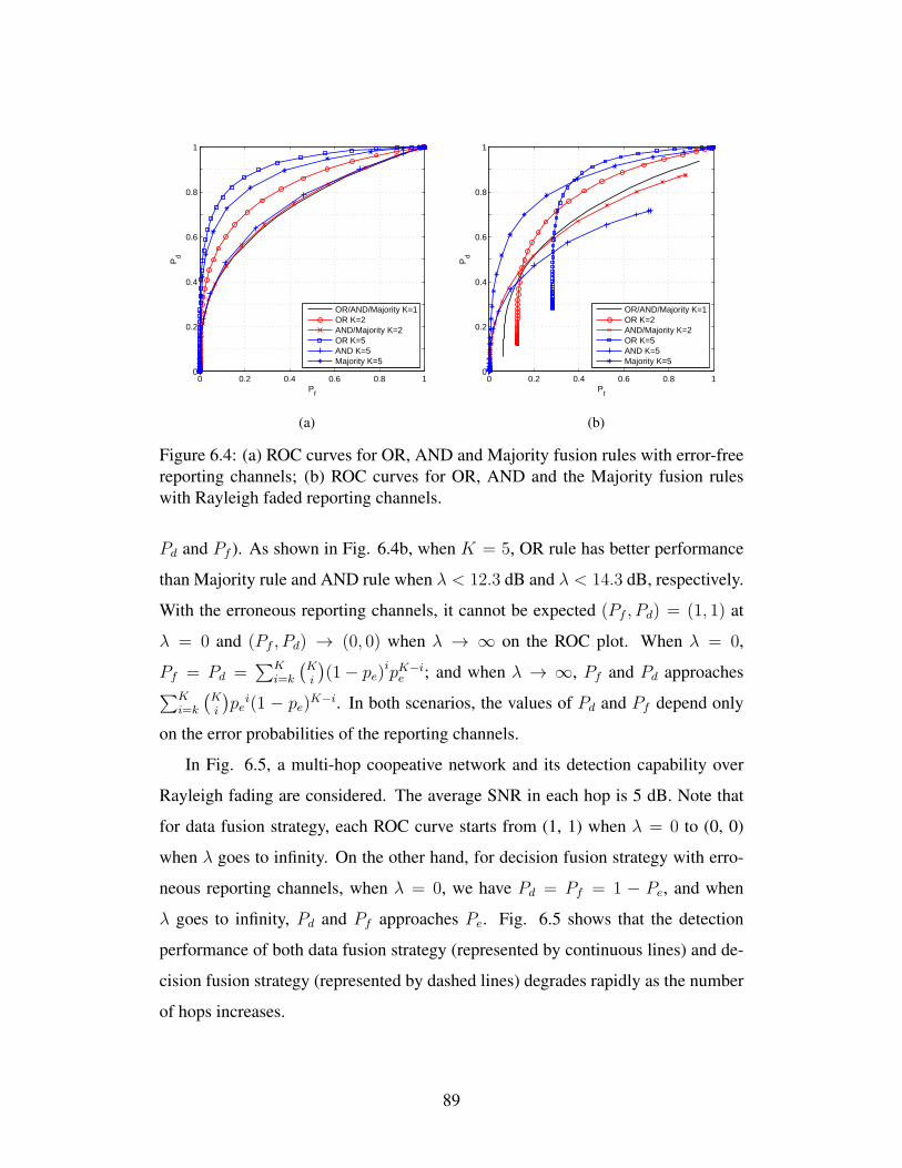
0 0.2 0.4 0.6 0.8 10
0.2
0.4
0.6
0.8
1
Pf
Pd
OR/AND/Majority K=1OR K=2AND/Majority K=2OR K=5AND K=5Majority K=5
(a)
0 0.2 0.4 0.6 0.8 10
0.2
0.4
0.6
0.8
1
Pf
Pd
OR/AND/Majority K=1OR K=2AND/Majority K=2OR K=5AND K=5Majority K=5
(b)
Figure 6.4: (a) ROC curves for OR, AND and Majority fusion rules with error-freereporting channels; (b) ROC curves for OR, AND and the Majority fusion ruleswith Rayleigh faded reporting channels.
Pd and Pf ). As shown in Fig. 6.4b, when K = 5, OR rule has better performance
than Majority rule and AND rule when λ < 12.3 dB and λ < 14.3 dB, respectively.
With the erroneous reporting channels, it cannot be expected (Pf , Pd) = (1, 1) at
λ = 0 and (Pf , Pd) → (0, 0) when λ → ∞ on the ROC plot. When λ = 0,
Pf = Pd =∑K
i=k
(Ki
)(1− pe)
ipK−ie ; and when λ → ∞, Pf and Pd approaches∑K
i=k
(Ki
)pe
i(1 − pe)K−i. In both scenarios, the values of Pd and Pf depend only
on the error probabilities of the reporting channels.
In Fig. 6.5, a multi-hop coopeative network and its detection capability over
Rayleigh fading are considered. The average SNR in each hop is 5 dB. Note that
for data fusion strategy, each ROC curve starts from (1, 1) when λ = 0 to (0, 0)
when λ goes to infinity. On the other hand, for decision fusion strategy with erro-
neous reporting channels, when λ = 0, we have Pd = Pf = 1 − Pe, and when
λ goes to infinity, Pd and Pf approaches Pe. Fig. 6.5 shows that the detection
performance of both data fusion strategy (represented by continuous lines) and de-
cision fusion strategy (represented by dashed lines) degrades rapidly as the number
of hops increases.
89

0 0.2 0.4 0.6 0.8 10
0.1
0.2
0.3
0.4
0.5
0.6
0.7
0.8
0.9
1
Pf
Pd
M = 1M = 2M = 3M = 4M = 5
Figure 6.5: ROC curves for a multi-hop cooperative network.
6.6 Conclusion
Detection performance of cooperative spectrum sensing is analyzed for data fusion
and decision fusion strategies. A new set of results is derived for the average de-
tection probability. For the data fusion strategy, the MGFs of received SNR of the
primary user’s signal at the fusion center are utilized to derive tight bounds of the
average detection probability. For the decision fusion strategy in the cooperative
spectrum sensing, the generalized k-out-of-n fusion rule is considered, with partic-
ular focus on the OR, AND, and Majority rules. OR rule always outperforms AND
and Majority rules, and Majority rule has better detection capability than AND rule
with error-free reporting channels. However, given a probability of reporting error,
the performance is limited by the reporting error. The detection performance of
both strategies degrades rapidly when the number of hops increases.
∼
90

Chapter 7
Energy Detection in Low SNR
The IEEE 802.22 standard requires spectrum-sensing techniques to identify pri-
mary signals with a very low SNR. In this chapter, under such low-SNR levels, the
detection performance of a conventional energy detector used for spectrum sensing
in cognitive radio networks is investigated. The analysis focuses on deriving ap-
proximations for two performance metrics: (1) the average missed-detection proba-
bility, and (2) the average AUC, which measures the overall detection capability of
an energy detector. The analysis develops a unified framework covering many ex-
isting fading channels, square-law diversity-combining technique and cooperative
spectrum-sensing scenarios. The detection threshold is also optimized to minimize
the total error rate subject to bounded false alarm and missed-detection probabili-
ties.
7.1 Introduction
In Section 2.6, some of the specifications of the IEEE 802.22 standard are given,
in which the requirements of false alarm and missed-detection probabilities (both
are less than 0.1) should be met with a very low SNR, e.g., -20 dB SNR [13].
Thus, spectrum sensing at low SNR is vital. Research on various spectrum sens-
ing techniques at moderate and high SNRs is frequently available in the litera-
ture [48, 53, 54]. However, research on spectrum sensing at low SNR is still very
limited. The low SNR spectrum sensing is considered for a differential energy de-
tection scheme of multi-carrier systems (e.g., OFDM) in [58], for multi-antenna
91

detectors (which improve the robustness to noise uncertainty) in [59, 60], and for
a covariance matrix based detection algorithm in [61]. Moreover, low-SNR coop-
erative spectrum sensing techniques are considered for belief propagation in [62],
for cyclostationary detection in [63], for optimal relaying scheme in [64], and for
multi-antenna with a noise-uncertainty-free detector in [65]. These works consider
generalized likelihood ratio detector, alternative energy detector, cyclostationary
feature detector or covariance based detector, in which the operating SNR ranges
generally from 0 to -30 dB.
Due to the mathematical complexity, none of the research in the literature pro-
vides a rigorous unified analytical framework (here ‘unified’ means the framework
is valid with most existing fading channels) for the performance analysis (e.g.,
on average detection performance) and parameter optimization (e.g., on detection
threshold or sensing time) for any spectrum sensing technique at low SNR. The
reason is that although the average performance metrics (e.g., average detection
probability) can be derived rigorously for some particular fading models, the same
analytical framework may not work well for the parameter optimization [53, 54].
Therefore, a unified analytical framework is critically important to the cognitive
radio industry and deserves full investigation, at least for the conventional energy
detection as a benchmark because it is the simplest detection technique and its per-
formance metrics can be an upper bound (e.g., on sensing time) or a lower bound
(e.g., on detection probability) for other complex detection techniques. To achieve
this, this chapter provides a basic rigorous unified analytical framework for con-
ventional energy detection over various fading channels, analyzes the detection
performance, derives the optimal detection threshold that minimizes the total er-
ror rate when both false alarm and missed-detection probabilities are bounded, and
investigates detection performance in diversity combining and cooperative sensing
scenarios.
The rest of this chapter is organized as follows. Section 7.2 discusses energy
detection and its low-SNR model. Section 7.3 analyzes the low-SNR performance
of an energy detector, in terms of the average missed-detection probability and the
average AUC. Sections 7.4 is devoted to the analysis of the optimal detection thresh-
92
old. Section 7.5 presents numerical and simulation results, followed by concluding
remarks in Section 7.6.
7.2 Low-SNR Model
Three signal models, S1, S2 and S3 which are given in Section 2.4.1, can be con-
sidered in the energy detection. For S1 and S2 signal models, the distribution of Λ
is modeled exactly in Section 2.4.2. Under H0, the false-alarm probability is with
the upper incomplete Gamma function. Under H1, the detection probabilities are
with the Marcum-Q function and with the upper incomplete Gamma function for
S1 and S2, respectively. However, none of these functions have closed-form inverse
functions, and thus there is no closed-form expression for the detection threshold
λ when a false-alarm or detection probability is given even with AWGN channel.
This problem becomes more complicated when the fading effect is considered. Al-
though there are rigorous expressions for the average detection performance over
some particular fading channels in the literature, such expressions may not help
for the parameter optimization (e.g., optimizing detection threshold). Since S1 and
S2 signal models have different set of expressions, results of one model cannot be
derived from those of the other model. Moreover, the distribution of Λ cannot be
modeled exactly for S3.
To solve all these problems, the CLT approach can be used as a unified approach
of accurately approximating the distribution of Λ in the three signal models. Re-
calling (2.23), the distribution of Λ can be approximated as a normal distribution
for sufficiently large N as
Λ ∼
N (N(2σ2
w), N(2σ2w)
2) : H0
N (N(2σ2w)(1 + γ), N(2σ2
w)2(1 + 2γ)) : H1 with S1 or S3
N (N(2σ2w)(1 + γ), N(2σ2
w)2(1 + γ)2) : H1 with S2.
(7.1)
Under the low-SNR assumption (i.e., γ ≪ 1), the signal has little impact on
the variance of the test statistic under H1, as used in the Edell model, Berkeley
model and Torrieri model which are well-known Gaussian approximations for the
test statistic under H1 [122, 123]. Thus, (7.1) can be accurately approximated for
93

any of the three signal models as
Λlow ∼
N (Nσ2, Nσ4) : H0
N (Nσ2(1 + γ), Nσ4) : H1(7.2)
where σ =√2σw. The false alarm probability Pf and the missed-detection proba-
bility Pmd(γ) can be evaluated as
Pf =1
2Erfc
(λ−Nσ2
√2Nσ2
)(7.3)
and
Pmd(γ) ≈ 1− 1
2Erfc
(λ−Nσ2(1 + γ)√
2Nσ2
), (7.4)
respectively, where where Q(z) = 12Erfc
(z√2
)and Erfc(·) is the complementary
error function defined as Erfc(z) = 2√π
∫∞ze−t2 dt [74]. Since the detection prob-
ability, Pd(γ) = 1− Pmd(γ), relates to the cumulative distribution function (CDF)
of the test statistic, Fig. 7.1 shows the exact CDF of the test statistic Λ, denoted
FΛ|H1,|h|(x), with S1 signal model and its low-SNR approximation for γ=-10 dB,
-15 dB, or -20 dB when σ = 1 and N = 2 × 10³. The exact CDF (solid line)
matches tightly with the approximation (discrete marks) for the simulated x range
at γ =-20 dB, while the other two cases also show close matches, confirming the
validity of the low-SNR approximation. The accuracy of the approximation is also
shown by the ROC curves in Fig. 7.2 (see discussion in Section 7.5).
7.3 Performance Analysis at a Low SNR
The MG channel model introduced in Chapter 4 is considered as a generalized SNR
distribution for the derivation of analytical results. The ROC curve, AUC, and the
total error rate are used as the performance measures. The ROC curve is a mea-
surement for the sensitivity of a detector used in a binary classifier system [124].
In signal-detection theory, the ROC (or the complementary ROC) curve is a graph-
ical plot of Pd(γ) (or Pmd(γ)) versus Pf as the discrimination threshold λ varies.
The ROC curves of spectrum-sensing detectors have highly non-linear behavior,
and they are, in general, convex. In wireless communications, Pd(γ) depends on
the received instantaneous SNR, which is a function of the mobile radio channel
94

1,900 2,000 2,100 2,200 2,3000
0.2
0.4
0.6
0.8
1
x
FΛ
|H1,|h
|(x)
ExactApproximation
− 15 dB
− 10 dB
− 20 dB
Figure 7.1: The exact and approximated (low-SNR) CDFs of the test statistic whichis modeled using the CLT, with σ = 1 and N = 2 × 10³. S1 is considered as anexample. The exact CDF is based on (7.1) and approximated CDF is based on (7.2).
gain. Therefore, the average detection probability (or average missed-detection
probability) over fading channels is important for plotting the ROC curve, which is
discussed in Section 7.3.1. The AUC is the area under the ROC curve, which varies
between 12
and 1. It represents the probability that the detector is more likely to
choose the correct decision than the incorrect decision. It is a single-valued mea-
sure for the overall detection capability of a detector. The average AUC can be
derived by averaging instantaneous AUC over the SNR distribution which is dis-
cussed in Section 7.3.2. The total error rate, denoted Pe, is the sum of the false
alarm and missed-detection probabilities, Pmd(γ) + Pf , which both depend on the
threshold λ. The total error rate is used in [125] (which is based on the S1 signal
model) as a possible metric for selecting λ. In this chapter, the total error rate is
also adopted to select λ, as will be discussed in Section 7.4.
In this section, a unified approach will be developed to evaluate average detec-
tion probability and average AUC at the low-SNR region. Diversity combining and
cooperative spectrum sensing are also investigated subsequently.
95

7.3.1 Average Missed-Detection ProbabilityOver Fading Channels
For fading channels, the average missed-detection probability, Pmd, can be cal-
culated by directly averaging Pmd(γ) over the SNR distribution to yield Pmd =∫∞0Pmd(x)fγ(x) dx. Next the MG channel model (4.1) will be used for SNR dis-
tributions of many existing fading channels, diversity-combining techniques, and
cooperative sensing.
With the aid of (7.4), (4.1), Erfc(−x) = 2− Erfc(x), and some straightforward
algebraic manipulations, the average missed-detection probability over the general-
ized channel model (4.1), PGenmd , can be given as
PGenmd ≈ 1
2
S∑i=1
αi
∞∫0
xβi−1e−ζixErfc
(√N
2x+
Nσ2 − λ√2Nσ2
)dx.
An integral expression, I(n, p, a, b), which will be used in the later analysis, is
defined as [126, eq. (2.8.9.1)]
I(n, p, a, b) ,∞∫0
xne−pxErfc(ax+ b) dx
=(−1)n∂n
∂pn
Erfc(b)− ep2+4pab
4a2 Erfc(b+ p
2a
)p
,(7.5)
where n is a positive integer, Re[p]> 0, a > 0, b > 0 , and ∂n
∂pn[·] is the nth-order
partial derivative with respect to p. Therefore, PGenmd can be derived for integer βi as
PGenmd ≈ 1
2
S∑i=1
αiI
(βi − 1, ζi,
√N
2,Nσ2 − λ√
2Nσ2
). (7.6)
For example, for a Rayleigh fading channel, the corresponding parameters are S =
1, α1 =1γ
, β1 = 1 and ζ1 = 1γ
. Thus, the average missed-detection probability over
the Rayleigh fading channel, P Raymd , is
P Raymd ≈ 1
2
[Erfc
(Nσ2 − λ√
2Nσ2
)− e
1γ2
+ 4γ
(Nσ2−λ√
2Nσ2
)√N2
2N Erfc(Nσ2 − λ√
2Nσ2+
1
γ√2N
)].
(7.7)
96
For a Nakagami-m fading channel, the corresponding parameters are S = 1, α1 =
mm
Γ(m)γm , β1 = m and ζ1 = mγ
. Thus, for integer m, the average missed-detection
probability over the Nakagami-m fading channel, PNakmd , is
PNakmd ≈ 1
2Γ(m)
(m
γ
)m
I
(m− 1,
m
γ,
√N
2,Nσ2 − λ√
2Nσ2
). (7.8)
Similarly, the average missed-detection probabilities over many other existing fad-
ing channels such as Nakagami-lognormal, K, KG, η-µ, Nakagami-q (Hoyt), κ-µ,
or Nakagami-n (Rician) can be derived easily after properly selecting the parame-
ters S, αi, βi, ζi (i = 1, 2, ..., S) in (4.1).
Diversity Reception
Since the traditional diversity techniques (e.g., MRC) may not work with energy
detection because coherent MRC needs channel state information, which increases
the system complexity, the SLC technique is considered. The outputs of the square-
law devices ofL branches are combined to yield a new decision statistic as in (5.23).
Note that, if Λi is a normal distribution as Λi ∼ N (µi, σ2i ), ΛSLC is also a normal
distribution as ΛSLC ∼ N(∑L
i=1 µi,∑L
i=1 σ2i
). Under H0 and H1, Λi is a normal
distribution as in (7.1) with γ replaced by γi (the SNR of the ith branch). For SLC
with a low SNR, the false alarm probability and the missed-detection probability
under AWGN channels can be evaluated as (7.3) and (7.4), respectively, with N
replaced by LN . For fading channels, if the PDF of γ = 1L
∑Li=1 γi is modeled
by using the generalized channel (4.1),1 with the aid of (7.6), the average missed-
detection probability can be derived as
PGen,SLCmd ≈ 1
2
S∑i=1
αiI
(βi − 1, ζi,
√LN
2,LNσ2 − λ√
2LNσ2
). (7.9)
Thus, the average missed-detection probability over a Rayleigh fading channel can
be derived by using (7.9) with S = 1, α1 = 1Γ(L)
(Lγ
)L, β1 = L and ζ1 = L
γ. Sim-
ilarly, the average missed-detection probability over a Nakagami-m fading channel
1As special cases, the PDF of γ = 1L
∑Li=1 γi when signals of the branches follow
i.i.d. Rayleigh and Nakagami-m fading is fγ(x) = 1Γ(L)
(Lγ
)LxL−1e−
Lγ x and fγ(x) =
1Γ(mL)
(mLγ
)mL
xmL−1e−mLγ x, respectively.
97

can be derived by using (7.9) with S = 1, α1 = 1Γ(mL)
(mLγ
)mL
, β1 = mL and
ζ1 =mLγ
.
If the square-law selection combining technique is applied, the average missed-
detection probability can be derived by using the results in [53] and the general
expression given in eq. (7.6).
Cooperative Spectrum Sensing
Cooperative spectrum sensing can improve signal detection capability by sharing
and combining the information from intermediate cognitive nodes (called coopera-
tive nodes). Because the existing research in the literature focuses on the medium-
or high-SNR region [116], the impact of cooperative spectrum sensing at a low
SNR has not been clarified. To investigate this case, the decision fusion strategy,
in which each cooperative node makes a decision on the primary user activity, is
considered and individual 1-bit decisions are reported to a fusion center. If there
are K cooperative nodes, and the fusion center uses the k-out-of-K fusion rule
(i.e., the fusion center decides on the presence of primary activity if there are k or
more cooperative nodes that individually decide on the presence of primary activ-
ity), the false alarm probability P Coopf and detection probability P Coop
d at the fusion
center can be written as P Coopχ =
∑Ki=k
(Ki
)(pχ)
i(1 − pχ)K−i, where the notation
‘χ’ means ‘f ’ or ‘d’ for false alarm or detection, respectively. It is assumed that
all cooperative nodes have i.i.d. channels from the primary user, and thus, achieve
identical false alarm probability pf and detection probability pd. Thus, the average
missed-detection probability of cooperative spectrum sensing over the generalized
channel model is
PGen,Coopmd ≈ 1−
K∑i=k
(K
i
)(PGenmd
)i (1− PGen
md
)K−i
, (7.10)
with PGenmd given in (7.6). For example, for a Nakagami-m channel, the average
missed-detection probability is equal to (7.10) with PGenmd replaced by PNak
md given in
(7.8).
98

7.3.2 Average AUC
A general expression for the area under the curve is derived in the following Theo-
rem 7.1 for the AWGN case.
Theorem 7.1 Two functions which depend on λ (−∞ < λ < ∞)2 are defined as
Pf (λ) = 12Erfc
(λ−m0√
2σ0
)and Pd(λ) = 1
2Erfc
(λ−m1√
2σ1
), where m0, m1, σ0, and σ1
are real positive values such that m0 ≤ m1 and σ0 ≤ σ1. By eliminating term λ, the
two functions can be combined as Pd = 12Erfc
(σ0
σ1Erfc−1(2Pf )− m1−m0√
2σ1
), which
represents the Pd versus Pf curve. Thus, the area under the Pd versus Pf curve, A,
is given as
A = 1− 1
2Erfc
(m1 −m0√2(σ2
0 + σ21)
). (7.11)
Proof: See Appendix D.1.
The instantaneous AUC of an energy detector at a low SNR can be derived from
(7.11) by replacing m0 = Nσ2, m1 = Nσ2(1 + γ), σ20 = Nσ4, and σ2
1 = Nσ4,
as A(γ) ≈ 1 − 12Erfc
(√N2γ)
. Then the average AUC over the generalized SNR
distribution (4.1) is derived as AGen =∫∞0
A(x)fγ(x) dx, to yield
AGen ≈ 1− 1
2
S∑i=1
αi
∫xβi−1e−ζixErfc
(√N
2x
)dx
= 1 +1
2
S∑i=1
(−1)βi−1αi∂βi−1
∂pβi−1
(1
pe
p2
N Erfc(
p√N
)− 1
p
) ∣∣∣∣∣p=ζi
,
(7.12)
where βi is a positive integer, and the second equality comes after applying [126, eq.
(2.8.5.4)]. This approximation can be used for many mobile radio channel models.
For example, the average AUC over a Rayleigh fading channel, ARay, is
ARay ≈ 1
2+e
1Nγ2
2Erfc
(1
γ
√1
N
), (7.13)
and the average AUC over a Nakagami-m fading channel, ANak, is
ANak ≈ 1 +(−1)m−1mm
2Γ(m)γm∂m−1
∂pm−1
(1
pe
p2
N Erfc(
p√N
)− 1
p
) ∣∣∣∣∣p=m
γ
, (7.14)
2This is the theoretical limit of λ, but negative values of threshold are not considered in practice.
99

where m is an integer.
For the SLC technique, , the average AUC over the generalized channel model is
given in (7.12) with N replaced by LN if the PDF of γ = 1L
∑Li=1 γi is modeled by
using the generalized channel. For example, the average AUC over Rayleigh fading
channels can be derived by using (7.12) with S = 1, α1 = 1Γ(L)
(Lγ
)L, β1 = L,
ζ1 = Lγ
and with N replaced by LN . Similarly, the average AUC over Nakagami-
m fading channels can be derived by using (7.12) with S = 1, α1 =1
Γ(mL)
(mLγ
)mL
,
β1 = mL, ζ1 = mLγ
and with N replaced by LN .
For cooperative spectrum sensing, because P Coopd is difficult to be expressed in
terms of P Coopf , the AUC may not be able to be evaluated even with some numer-
ical methods. Alternatively, a threshold averaging approach which gives the AUC
as A = −∫∞−∞ Pd(λ)
∂Pf (λ)
∂λdλ may be used, because the threshold, λ, affects the
false alarm, the detection and the missed-detection probabilities, which are hence
denoted as Pf (λ), Pd(λ) and Pmd(λ), respectively. By using the binomial expan-
sion and the fact that ∂∂x
[Erfc
(x−ab
)]= − 2
b√πe−
(x−a)2
b2 , the AUC of cooperative
spectrum sensing can be expressed in an integral, which can be evaluated by nu-
merical methods. However, a closed-form expression appears difficult. Note that
our analytical approach for the average missed-detection probability and the aver-
age AUC can also be applied to other alternative energy detection methods in which
the energy detector test statistic is modeled as Gaussian via the CLT.
7.4 Threshold Selection
The traditional way of threshold selection is based on the false alarm probability
only. For a given number of samples (N ), estimated noise variance (σ2), and the
allowable false alarm probability (Pf ), the threshold can thus be obtained by us-
ing (7.3) as λ =(√
2Erfc−1(2Pf ) +√N)√
Nσ2. Unfortunately, this threshold
selection method is not suitable for cognitive radio networks where it is essential
to keep a low missed-detection probability such that primary users are protected
from interference. While threshold selection with different objective functions (by
relaxing some constraints) has been performed in [67,127] and among others, these
100

papers focus on non-fading scenarios because the optimal threshold is analytically
intractable over fading channels. Moreover, the average missed-detection proba-
bility over fading channels has not been available for the low SNR model in (7.2).
Therefore, threshold selection that takes missed-detection probability into account
for the low SNR model over fading channels has not been studied previously, and
is the focus of this section.
For a cognitive radio network, Pmd(λ) is required to be no more than a threshold
denoted P thmd (e.g., Pmd(λ) ≤ 0.1 is required in the IEEE 802.22). This requirement
is equivalent to λ ≤ λ∗md where Pmd(λ∗md) = P th
md, since Pmd(λ) increases with
threshold λ. In addition, it may be required that Pf (λ) is no more than a threshold
P thf (e.g., Pf (λ) ≤ 0.1 is required in the IEEE 802.22) such that the spectrum
opportunities are efficiently utilized. This requirement is equivalent to λ ≥ λ∗f
where Pf (λ∗f ) = P th
f , since Pf (λ) decreases with threshold λ.3
If λ∗f > λ∗md, then there is no feasible λ that satisfies both requirements on
false alarm and missed-detection probabilities, which means other actions need to
be taken, such as increasing the sampling rate of the received signal. If λ∗f ≤ λ∗md,
this means any λ value within range [λ∗f , λ∗md] can satisfy both requirements on false
alarm and missed-detection probabilities. To select a value in the range [λ∗f , λ∗md], a
combination metric of both Pf (λ) and Pmd(λ) can be considered. For this purpose,
the Bayesian cost [128], which is a popular metric to select the detection threshold
in the literature [125, 129–131], can be used. If no cost is associated with correct
decisions on H0 and H1, the Bayesian cost function can be given as
R(λ) = C01P0Pf (λ) + C10P1Pmd(λ),
where C01 and C10 are cost associated with false alarm and missed-detection, re-
spectively, and P0 and P1 are probabilities of H0 and H1, respectively. Since it may
not be reasonable for secondary users to know P0 and P1 in advance, it can be set
P0 = P1, and also set C01 = C10. Then minimizing the Bayesian cost is equiva-
lent to minimizing the total error rate Pe(λ)= Pf (λ) + Pmd(λ).4 Therefore, the
3Note that if P thf = 1, it is equivalent to the case with no requirement on false alarm probability,
which means λ∗f = 0.
4Please note that, if the secondary users know P0 and P1, and/or C01 = C10, our method for the
101

threshold selection problem is formulated as
minimizeλ
Pe(λ) = Pf (λ) + Pmd(λ)
subject to Pf (λ) ≤ P thf
Pmd(λ) ≤ P thmd.
(7.15)
In the optimization problem in (7.15), if the two constraints are relaxed, denote
the optimal solution as λ∗e. Then the optimal solution for problem (7.15), denoted
λ∗, is given as
• λ∗ = λ∗e if λ∗f ≤ λ∗md and λ∗e ∈ [λ∗f , λ∗md];
• λ∗ = λ∗f or λ∗md, whichever is closer to λ∗e, if λ∗f ≤ λ∗md and λ∗e /∈ [λ∗f , λ∗md];
• λ∗ has no solution if λ∗f > λ∗md.
Since Pf (λ) does not depend on fading effect, λ∗f can be derived for any fading
scenario by using (7.3) as
λ∗f =
(√2
NErfc−1
(2P th
f
)+ 1
)Nσ2. (7.16)
In the following, exact λ∗md and λ∗e for AWGN channels and approximated λ∗md and
λ∗e are derived for Rayleigh fading channels.
AWGN Channel
For an AWGN channel, the general case for test statistic Λ in (2.23) is considered.
For S1 or S3 signal model with any SNR value γ, λ∗md can be derived by using
(2.23) as
λ∗md =
(√2(1 + 2γ)
NErfc−1
(2(1− P th
md))+ (1 + γ)
)Nσ2, (7.17)
and λ∗e is given by using (2.23) as
λ∗e = arg minλ
(1 +
1
2Erfc
(λ−Nσ2
√2Nσ2
)− 1
2Erfc
(λ−Nσ2(1 + γ)√2N(1 + 2γ)σ2
))
=Nσ2
2
(1 +
√1 + 2γ
(1 +
(1 + 2γ) ln(1 + 2γ)
Nγ2
) ) (7.18)
optimal threshold selection also works, which minimizes the corresponding Bayesian cost subjectto bounded false alarm and missed-detection probabilities.
102
where the second equality comes as explained in Appendix D.2. Similarly, λ∗md and
λ∗e for S2 signal model can be derived as
λ∗md =
(√2
N(1 + γ)Erfc−1
(2(1− P th
md))+ (1 + γ)
)Nσ2,
λ∗e =Nσ2
2
(1 +
√1 +
2(2 + γ) ln(1 + γ)
Nγ
)(1 + γ
1 + γ2
).
(7.19)
Rayleigh Fading Channel
For a Rayleigh fading channel with low-SNR value, the exact λ∗md and λ∗e are dif-
ficult to be derived due to the non-linearity of Pmd(λ) = P Raymd (λ) and Pe(λ) =
Pf (λ) + P Raymd (λ), respectively, where P Ray
md (λ) is given in (7.7). They can be cal-
culated numerically by using mathematical software packages (e.g., MATHEMAT-
ICA and MATLAB). Here approximations for λ∗md and λ∗e are derived.
Defining α = Nσ2−λ
Nσ2γand a
= 1√2Nγ
, (7.7) can be written as
P Raymd (λ) ≈
1
2
[Erfc (α)− ea
2
e2aαErfc (a+ α)
]. (7.20)
Over an AWGN channel at low SNR, it can be observed from (7.18) that, at a low
SNR (i.e., γ ≪ 1, 1+2γ ≈ 1) and a large N (note that reliable detection is possible
at a large N ), λ∗e can roughly be approximated as λ∗e ≈ Nσ2
2
(1 +
√1 + 2γ
).5 This
rough information is used to find approximated λ∗md and λ∗e for Rayleigh fading. By
using the Taylor series expansions of the Erfc(x) and e2axErfc(a+x) at zero where
Erfc(x) = 1− 2x√π+
2x3
3√π+O(x4)
and
e2axErfc(a+ x) =Erfc(a) +
(2aErfc(a)− 2e−a2
√π
)x
+
(2a2Erfc(a)− 2ae−a2
√π
)x2 +O(x3),
5Here we consider S1 or S3 signal model, as S2 signal model can be treated similarly.
103

P Raymd (λ) can be expanded when α → 0 as
P Raymd (λ) ≈
1
2
(1− ea
2
Erfc(a))− aea
2
Erfc(a)α
+
(a√π− a2ea
2
Erfc(a))α2 +O(α3).
(7.21)
Setting P Raymd (λ
∗md) = P th
md, λ∗md can be calculated as
λ∗md ≈
(1−
√2
Nα∗
)Nσ2 (7.22)
where α∗ =
(A−π1/4
√(4P th
mda−2a− A√π (2a(2P
thmd−1)
√π+A−2)
))2a(1−A)
andA =√πaea
2Erfc(a).
The total error rate is Pe(λ) = Pf (λ) +P Raymd (λ). For ∂Pe(λ)
∂λ= 0, with the aid of
(7.3) and (7.7), it can be written
∂Pe(λ)
∂λ=e
12Nγ2
−λ−Nσ2
Nσ2γ Erfc(
1√2Nγ
− λ−Nσ2√2Nσ2
)2Nσ2γ
− e−(λ−Nσ2)2
2Nσ4
√2πNσ2
= 0
⇐⇒ e
(1√2Nγ
−λ−Nσ2√
2Nσ2
)2
Erfc(
1√2Nγ
− λ−Nσ2
√2Nσ2
)=
√2N
πγ.
(7.23)
The argument of the exponential function and the complementary error function
Erfc(·) in the second line of (7.23), denoted as x =(
1√2Nγ
− λ−Nσ2√2Nσ2
), becomes
very small when N is large.6 Therefore, the Taylor series expansions of these two
functions are considered at zero, which are ex2= 1+x2+ x4
2+O(x6) and Erfc(x) =
1− 2x√π+ 2x3
3√π+O(x5) when x→ 0. Define function
g(x) , ex2
Erfc(x) = 1− 2x√π+ x2 − 4x3
3√π+x4
2− 8x5
15√π+O(x6). (7.24)
Now g(x) = c is to be solved where c =√
2Nπγ as in (7.23). If the first two terms
of (7.24) are considered, we have x ≈√π2(1− c), which leads to
λ∗e ≈2√π
(1 + γ +
1
Nγ−√
π
2N
)Nσ2.
6On the other hand, if N is small, the argument of the exponential function and the comple-mentary error function Erfc(·) in the second line of (7.23) may approach to a large value.Therefore, the Taylor series expansion of Erfc(x) around infinity can be considered, given asErfc(x) = e−x2
(1√πx
− 12√πx3 + 3
4√πx5 +O
(1x6
))when x → ∞. Thus it can be written
g(x) = ex2
Erfc(x) = 1√πx
− 12√πx3 + 3
4√πx5 + O
(1x6
). Similar to the case with large N , a
more accurate approximation for λ∗e can be found by keeping increasing the number of terms of
g(x).
104
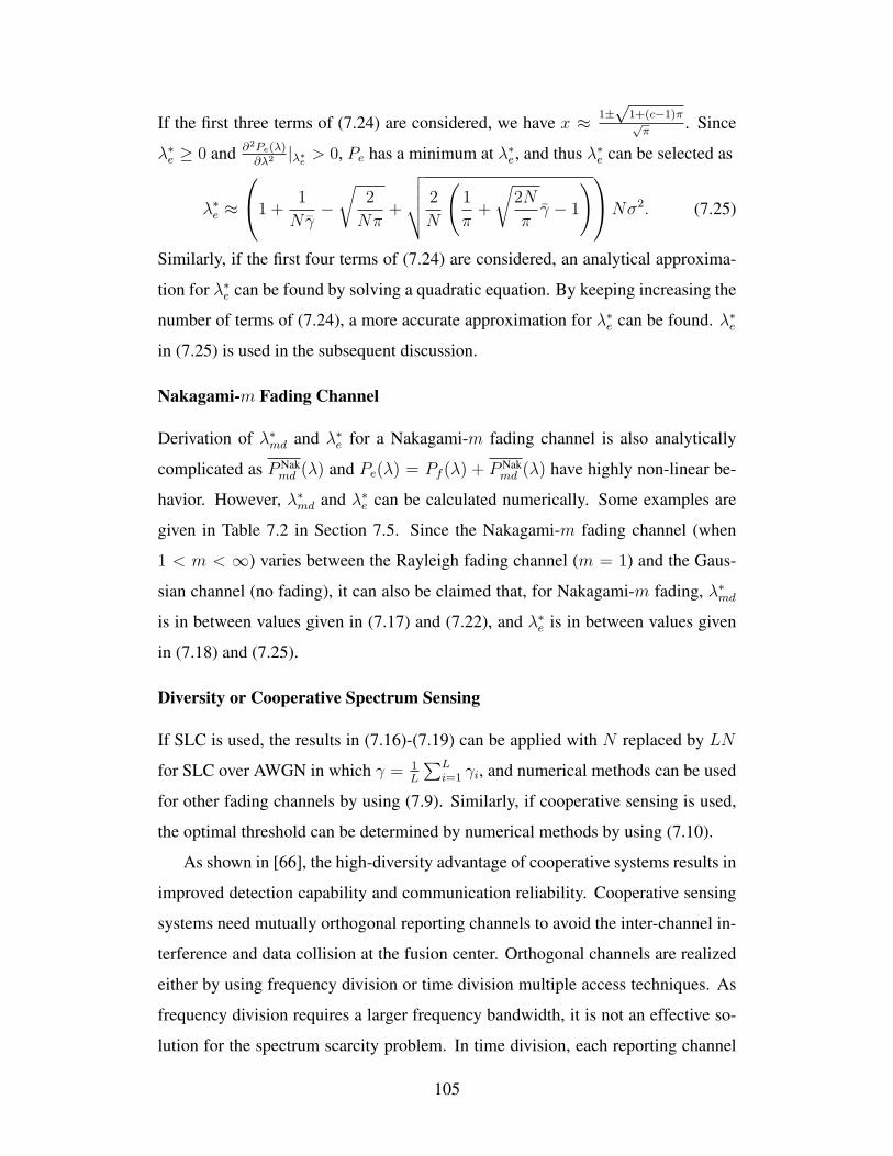
If the first three terms of (7.24) are considered, we have x ≈ 1±√
1+(c−1)π√π
. Since
λ∗e ≥ 0 and ∂2Pe(λ)∂λ2 |λ∗
e> 0, Pe has a minimum at λ∗e, and thus λ∗e can be selected as
λ∗e ≈
1 +1
Nγ−√
2
Nπ+
√√√√ 2
N
(1
π+
√2N
πγ − 1
)Nσ2. (7.25)
Similarly, if the first four terms of (7.24) are considered, an analytical approxima-
tion for λ∗e can be found by solving a quadratic equation. By keeping increasing the
number of terms of (7.24), a more accurate approximation for λ∗e can be found. λ∗ein (7.25) is used in the subsequent discussion.
Nakagami-m Fading Channel
Derivation of λ∗md and λ∗e for a Nakagami-m fading channel is also analytically
complicated as PNakmd (λ) and Pe(λ) = Pf (λ) + PNak
md (λ) have highly non-linear be-
havior. However, λ∗md and λ∗e can be calculated numerically. Some examples are
given in Table 7.2 in Section 7.5. Since the Nakagami-m fading channel (when
1 < m < ∞) varies between the Rayleigh fading channel (m = 1) and the Gaus-
sian channel (no fading), it can also be claimed that, for Nakagami-m fading, λ∗md
is in between values given in (7.17) and (7.22), and λ∗e is in between values given
in (7.18) and (7.25).
Diversity or Cooperative Spectrum Sensing
If SLC is used, the results in (7.16)-(7.19) can be applied with N replaced by LN
for SLC over AWGN in which γ = 1L
∑Li=1 γi, and numerical methods can be used
for other fading channels by using (7.9). Similarly, if cooperative sensing is used,
the optimal threshold can be determined by numerical methods by using (7.10).
As shown in [66], the high-diversity advantage of cooperative systems results in
improved detection capability and communication reliability. Cooperative sensing
systems need mutually orthogonal reporting channels to avoid the inter-channel in-
terference and data collision at the fusion center. Orthogonal channels are realized
either by using frequency division or time division multiple access techniques. As
frequency division requires a larger frequency bandwidth, it is not an effective so-
lution for the spectrum scarcity problem. In time division, each reporting channel
105
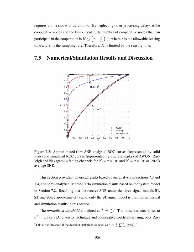
requires a time slot with duration τr. By neglecting other processing delays at the
cooperative nodes and the fusion center, the number of cooperative nodes that can
participate in the cooperation is K ≤(τ − N
fs
)1τr
, where τ is the allowable sensing
time and fs is the sampling rate. Therefore, K is limited by the sensing time.
7.5 Numerical/Simulation Results and Discussion
0 0.1 0.2 0.3 0.4 0.5 0.6 0.7 0.8 0.9 10
0.1
0.2
0.3
0.4
0.5
0.6
0.7
0.8
0.9
1
Pf
Pd
AWGNRayleighNakagami−4
N=2×10⁵
N=2×10³
Figure 7.2: Approximated (low-SNR analysis) ROC curves (represented by solidlines) and simulated ROC curves (represented by discrete marks) of AWGN, Ray-leigh and Nakagami-4 fading channels for N = 2× 10³ and N = 2× 10⁵ at -20 dBaverage SNR.
This section provides numerical results based on our analysis in Sections 7.3 and
7.4, and semi-analytical Monte-Carlo simulation results based on the system model
in Section 7.2. Recalling that the receive SNR under the three signal models S1,
S2, and S3are approximately equal, only the S1 signal model is used for numerical
and simulation results in this section.
The normalized threshold is defined as λ , λN
.7 The noise variance is set to
σ2 = 1. For SLC diversity technique and cooperative spectrum-sensing, only Ray-
7This is the threshold if the decision statistic is selected as Λ = 1N
∑Nn=1 |y(n)|
2.
106

0 0.2 0.4 0.6 0.8 10
0.1
0.2
0.3
0.4
0.5
0.6
0.7
0.8
0.9
1
Pf
Pd
SLC L=2SLC L=3Cooperative K=2Cooperative K=3
N=2×10³
N=2×10⁶
Figure 7.3: Approximated (low-SNR analysis) ROC curves (represented by solidlines) and simulated ROC curves (represented by discrete marks) of SLC whenL = 2, 3 and cooperative spectrum sensing when K = 2, 3 for N = 2 × 10³ andN = 2× 10⁶ over Rayleigh fading at -20 dB average SNR.
leigh fading channels are considered. The Rayleigh fading case provides a worst-
case benchmark because performance loss in Rayleigh fading channel is much
higher than those of AWGN and Nakagami-m (m > 1) fading channels.
One of the main contributions of this research is to derive analytical approx-
imations for the average missed-detection probability in a low-SNR region. The
analytical results can be used to plot ROC curves. Fig. 7.2 and Fig. 7.3 show the
ROC curves calculated based on the analytically derived approximations given in
(7.4), (7.7)-(7.10), and the simulated ROC curves. Specifically, Fig. 7.2 shows the
ROC curves for three fading scenarios: the AWGN, Rayleigh and Nakagami-4 fad-
ing channels with -20 dB average SNR. The ROC curves are plotted in the range
λ ∈ [0.95, 1.05] and λ ∈ [0.995, 1.02] for N = 2 × 10³ and N = 2 × 10⁵, re-
spectively. Fig. 7.3 shows the ROC curves of the SLC diversity technique with
L = 2, 3 and cooperative spectrum-sensing network (with OR decision fusion
rule) with K = 2, 3 over Rayleigh fading at γ= -20 dB when N takes two val-
ues: when N = 2 × 10³, the ROC curves are plotted in the range λ ∈ [1.92, 2.10]
107

and λ ∈ [2.94, 3.10] for SLC with L = 2 and 3, respectively, and in the range
λ ∈ [0.95, 1.1] for cooperative spectrum sensing; when N = 2 × 10⁶, the ROC
curves are plotted in the range λ ∈ [2.00, 2.02] and λ ∈ [3.00, 3.03] for SLC with
L = 2 and 3, respectively, and in the range λ ∈ [0.99, 1.03] for cooperative spec-
trum sensing. The analytical results perfectly match the simulation results for a high
and low number of samples, and also for high and low Pd and Pf , confirming the
accuracy of our low-SNR approximations in (7.4), (7.7)-(7.10). From the two fig-
ures, it can be seen that, when N = 2× 10³, the IEEE 802.22 requirements on false
alarm and missed-detection probabilities cannot be satisfied simultaneously in any
case in the two figures; when N = 2×10⁵, the requirements can be satisfied simul-
taneously for all cases in Fig. 7.2 except Rayleigh fading case; when N = 2× 10⁶,
the requirements can be satisfied simultaneously for all cases in Fig. 7.3. The two
figures clearly show that a larger N improves detection performance. Moreover,
the detection capability is significantly increased with L and K due to the effect of
diversity advantage.
Another contribution of this research is to derive approximations for the average
low-SNR AUC. For example, in Fig. 7.2, the three ROC curves withN = 2×10³ in-
tersect each other, making it difficult to compare the overall detection performance
among the three fading scenarios. In such a case, the AUC, a single-valued mea-
surement, is a better comparative performance metric. By using the approximations
given in Section 7.3.2, the average AUCs with different fading channels and with
SLC diversity combining are calculated and included in Table 7.1. In this table, the
numbers in brackets are area under the simulated curves in Fig. 7.2 and Fig. 7.3. It
can be seen that our approximations for AUC are accurate. As expected, AUC of
energy detection over AWGN channel and that over Rayleigh fading channel vary
from the largest to the smallest. With SLC, a larger number of branches leads to
a higher AUC and provides better overall detection capability. Obviously, a larger
number of samples also leads to a higher AUC confirming a better overall detection
capability.
The next contribution of this research is that the optimal threshold, λ∗, is de-
termined by minimizing the total error rate, Pe(λ) = Pf (λ) + Pmd(λ) under con-
108
Fig. 7.2 N = 2× 10³ N = 2× 10⁵ Fig. 7.3 N = 2× 10³ N = 2× 10⁶
AWGN 0.624085 (0.623489) 0.999217 (0.999174) SLC L = 2 0.663636 (0.662751) 0.995683 (0.995679)Nakagami-4 0.622408 (0.62172) 0.974777 (0.97462) SLC L = 3 0.698242 (0.697292) 0.999455 (0.999455)
Rayleigh 0.616163 (0.615361) 0.895188 (0.895034)
Table 7.1: AUC approximations (the numbers in front of the brackets) versus thearea under the simulated curves (the numbers in the brackets) for AWGN, Rayleigh,Nakagami-4 channels in Fig. 7.2 and SLC (L = 2, 3) in Fig. 7.3.
0.995 1 1.005 1.01 1.015 1.02 1.0250
0.1
0.2
0.3
0.4
0.5
0.6
0.7
0.8
0.9
1
Normalized threshold
Pe
AWGNRayleighNakagami−4Cooperative K=2
(a)
2.995 3 3.005 3.01 3.015 3.02 3.0250
0.1
0.2
0.3
0.4
0.5
0.6
0.7
0.8
0.9
1
Normalized threshold
Pe
SLC L=3
(b)
Figure 7.4: Approximated total error rate (represented by solid lines) and simu-lated total error rate (represented by discrete marks) versus normalized thresholdof (a) AWGN, Rayleigh and Nakagami-4 channels and cooperative spectrum sens-ing (K = 2) over Rayleigh fading; (b) SLC (L = 3) over Rayleigh fading, forN = 2× 10⁶ at -20 dB average SNR.
straints Pf (λ) ≤ P thf , Pmd(λ) ≤ P th
md. We denote P ∗e = Pe(λ
∗), P ∗f = Pf (λ
∗), and
P ∗md = Pmd(λ
∗). When γ= -20 dB and N = 2 × 10⁶, Fig. 7.4a and Fig. 7.4b
show low-SNR approximated total error rates (analytical results represented by
solid lines, where the average missed-detection probability is calculated based on
our analysis in Section 7.3.1) and simulated total error rates (represented by discrete
marks) versus the normalized threshold for the AWGN, Rayleigh, Nakagami-4 fad-
ing channels, cooperative spectrum sensing (K = 2), and SLC diversity combin-
ing (L = 3). Since the analytical results perfectly match the simulation results
in Fig. 7.4, Table 7.2 shows only the numerically calculated normalized thresh-
old values (λ∗f , λ∗md, λ∗e, λ∗), and numerically calculated false alarm probability,
missed-detection probability, and total error rate at λ∗e. In Table 7.2, the numbers
109

SLC L = 3 Cooperative K = 2AWGN Rayleigh Nakagami-4 over Rayleigh over Rayleigh
λ∗f 1.00091 1.00091 1.00091 3.00157 1.00116λ∗md 1.00908 1.00106 (1.0010) 1.00429 3.01096 1.00383λ∗e 1.00498 1.00138 (1.0027) 1.00190 3.00357 1.00192
Pf (λ∗e) 9.90× 10⁻¹³ 0.02 0.004 0.002 0.007
Pmd(λ∗e) 9.90× 10⁻¹³ 0.13 0.011 0.007 0.030
Pe(λ∗e) 1.98× 10⁻¹² 0.15 0.015 0.009 0.037
λ∗ λ∗e λ∗md λ∗e λ∗e λ∗e
Table 7.2: Numerically calculated normalized threshold values (λ∗f , λ∗md, λ∗e, λ∗)
and numerically calculated error probabilities (Pf , Pmd, Pe) at λ∗e for AWGN,Rayleigh and Nakagami-4 channels, SLC, and cooperative spectrum sensing whenN = 2× 10⁶ and γ = −20 dB. The numbers in brackets are approximated λ∗md andλ∗e for Rayleigh fading channels based on (7.22) and (7.25).
in brackets are approximated λ∗md and λ∗e for Rayleigh fading channels based on
(7.22) and (7.25).8 From Table 7.2, we have λ∗f < λ∗e < λ∗md for AWGN channel,
Nakagami-4 channel, SLC diversity combining, and cooperative sensing, and thus,
λ∗ = λ∗e. However, for Rayleigh channel, λ∗f < λ∗md < λ∗e, and thus, λ∗ = λ∗md.
In the rest of this section, the IEEE 802.22 requirements for spectrum sensing
are focused on by using standard parameter values. The IEEE 802.22 requirements
specify that Pf ≤ 0.1 and Pmd ≤ 0.1, and that the channel sensing time τ ≤ 2
seconds for any detection technique. Since N ≈ τfs where fs is the sampling
rate, which may depend on the sampling frequency of the ADC and the fast Fourier
transform bin resolution, N cannot be increased beyond τfs. In an experimental
energy detection implementation [57], fs is selected as fs = 62.5 kHz which may
be a typical test-bed bin resolution for moderate or high SNR. However, fs can take
several mega-hertz in other typical system implementations, e.g., some advanced
ADCs can operate at fs = 20MHz [132], 500 MHz [133], which may benefit low-
SNR sensing. In this chapter, we limit fs = 1MHz, and thus the maximal value of
N is 2× 10⁶ for 2 seconds of sensing time.9
Fig. 7.5 and Fig. 7.6 show analytical error rates (represented by lines) and sim-
8For AWGN channels, there is exact analytical solution for λ∗md and λ∗
e as given in (7.17) and (7.18).For Nakagami-m channels and for SLC or cooperative sensing over fading channels, there are noanalytical results for λ∗
md and λ∗e .
9As only sensing but not the subsequent processing is considered, 2 seconds is used as a referencesensing time. For a fixed N , sensing time can be proportionally reduced by using a higher samplingrate, e.g., there are 2× 10⁶ samples within 10 milliseconds at fs = 200MHz as in [134].
110

6.5 7 7.5 8 8.5 9 9.5 10
x 104
0.05
0.1
0.15
0.2
NP
roba
bilit
y
(a) AWGN
1.5 1.6 1.7 1.8 1.9 2
x 106
0.05
0.1
0.15
0.2
N
Pro
babi
lity
(b) Rayleigh
1.4 1.5 1.6 1.7 1.8 1.9 2 2.1 2.2
x 105
0.05
0.1
0.15
0.2
N
Pro
babi
lity
(c) Nakagami−4
Pf*
Pmd*
Pe*
N=205433
Ns=1511174
Ns=144842
Ns=66345
N=66748
Figure 7.5: Analytical error rates (represented by lines) and simulated error rates(represented by discrete marks) at the optimal threshold value (total error: P ∗
e ; falsealarm: P ∗
f ; and missed-detection: P ∗md) versus the number, N , of samples at -20 dB
average SNR for (a) AWGN; (b) Rayleigh; (c) Nakagami-4 fading channels.
ulated error rates (represented by discrete marks) at the optimal threshold (P ∗f =
Pf (λ∗), P ∗
md = Pmd(λ∗), and P ∗
e = Pe(λ∗)) versus N for fading channels (AWGN,
Rayleigh and Nakagami-4), diversity technique (SLC) and cooperative spectrum
sensing with -20 dB average SNR. The optimal threshold, λ∗, is calculated based
on low-SNR analysis in Section 7.4. Recall that an optimal threshold can be found
only when λ∗f ≤ λ∗md, which is equivalent to N ≥ Ns where Ns is the minimum
number of samples to have a feasible detection threshold that satisfies both require-
ments on false alarm and missed-detection probabilities. Under this condition, there
may be three possible cases such as (i) λ∗f ≤ λ∗md ≤ λ∗e; (ii) λ∗f ≤ λ∗e ≤ λ∗md; or (iii)
λ∗e ≤ λ∗f ≤ λ∗md. As examples given in Fig. 7.5 and Fig. 7.6, we do not have the
third case.
111

0.5 1 1.5 2 2.5 3
x 105
0
0.02
0.04
0.06
0.08
0.1
0.12
0.14
0.16
0.18
0.2
N
Pro
babi
lity
L=2L=3
Pf*
Pmd*
Pe*
Ns=62359 N
s=156005
N=96277
N=279606
(a)
0.5 1 1.5 2 2.5 3 3.5 4
x 105
0.02
0.04
0.06
0.08
0.1
0.12
0.14
0.16
0.18
0.2
N
Pro
babi
lity
K=2K=3
N=295948
N=109651
Pe*
Pf*
Pmd*
Ns=164897
Ns=70743
(b)
Figure 7.6: Analytical error rates (represented by lines) and simulated error rates(represented by discrete marks) at the optimal threshold value (total error: P ∗
e ; falsealarm: P ∗
f ; and missed-detection: P ∗md) versus the number, N , of samples at -20 dB
average SNR for (a) SLC when L = 2, 3; (b) cooperative spectrum sensing whenK = 2, 3, over Rayleigh fading.
Based on our analytical results in Fig. 7.5 and Fig. 7.6,10 the regions of N for
different possible cases are shown in Table 7.3. Table 7.3 also includes the minimal
sensing time to have a feasible detection threshold when fs = 1 MHz, given as
τmin = Ns
1 MHz , and the minimal sampling rate to have a feasible detection threshold
when the sensing time is 2 seconds, given as fs,min = Ns
2 sec . Two cases are used in
Fig. 7.5: AWGN and Rayleigh fading cases, as examples. For the AWGN channel,
there is no feasible detection threshold when N < Ns = 66345. When N ∈
[66345, 66747], we have λ∗f ≤ λ∗md ≤ λ∗e, the optimal threshold is determined by the
missed-detection probability requirement, and thus, in this region of N , P ∗md keeps
at 0.1. When N ≥ 66748, we have λ∗f ≤ λ∗e ≤ λ∗md, and the optimal threshold is
determined by minimizing the total error rate. For Rayleigh fading channel, there
is no feasible detection threshold when N < Ns = 1511174. When N varies from
Ns to 2× 10⁶ (the maximal number of samples when fs = 1 MHz and sensing time
τ = 2 seconds), we have λ∗f ≤ λ∗md ≤ λ∗e, and the optimal threshold is determined
10Since analytical and simulation results in Fig. 7.5 and Fig. 7.6 perfectly match, only the analyticalresults are used to generate Table 7.3.
112

by the missed-detection probability requirement, and thus, P ∗md keeps at 0.1 in this
region of N .
N τmin (sec) fs,min (kHz)λ∗f > λ∗md λ∗f ≤ λ∗md ≤ λ∗e λ∗f ≤ λ∗e ≤ λ∗md λ∗e ≤ λ∗f ≤ λ∗md at fs = 1MHz at τ = 2 sec
AWGN ≤ 66344 [66345, 66747] ≥ 66748 – 0.07 33.2Rayleigh ≤ 1511173 [1511174, 3871892] ≥ 3871893 – 1.51 755.6
Nakagami-4 ≤ 144841 [144842, 205432] ≥ 205433 – 0.14 72.4SLC L = 2 ≤ 156004 [156005, 279605] ≥ 279606 – 0.16 78.0SLC L = 3 ≤ 62358 [62359, 96276] ≥ 96277 – 0.06 31.2
Cooperative K = 2 ≤ 164896 [164897, 295947] ≥ 295948 – 0.16 82.4Cooperative K = 3 ≤ 70742 [70743, 109650] ≥ 109651 – 0.07 35.4
Table 7.3: The regions of N for different cases of λ∗f , λ∗md, λ
∗e, the minimal sensing
time τmin at fs = 1 MHz, and the minimal sampling rate fs,min at τ = 2 seconds.
In the following, diversity-combining technique (SLC with L = 2, 3) and coop-
erative spectrum sensing (K = 2, 3) are evaluated, which can be used to increase
the effective number of samples in the decision statistic while maintaining a small
value of the sampling rate. The Rayleigh fading channel is considered to establish
worse case scenario (than AWGN and Nakagami-m channels). From Table 7.3, for
two or three diversity branches in SLC,Ns is reduced fromNs =1511174 (no diver-
sity) to Ns =156005 or 62359, respectively, which results in the minimum sensing
time at fs = 1 MHz as τmin ≈ 0.16 or 0.06 seconds, and the minimal sampling
rate at τ = 2 seconds as fs,min ≈ 78.0 kHz or 31.2 kHz, respectively. Similarly, for
two or three cooperative nodes in a cooperative spectrum sensing network with OR
fusion rule, the minimum sensing time is τmin ≈ 0.16 or 0.07 seconds, and the min-
imal sampling rate is fs,min ≈ 82.4 kHz or 35.4 kHz, respectively. Thus, to satisfy
both IEEE 802.22 requirements on false alarm and missed-detection probabilities,
diversity combining and cooperative spectrum sensing can significantly reduce the
required sensing time and/or the required sampling rate. Note that, for diversity
combining and cooperative spectrum sensing, different processing delays may be
needed in different networks, which is not accounted in this research.
7.6 Conclusion
In this chapter, low-SNR energy detection in cognitive radio networks is studied.
New approximated expressions for the average missed-detection probability and the
113

average AUC over a generalized channel model are derived. The optimal detection
threshold problem is formulated to minimize the total error rate subject to bounded
false alarm and miss-detection probabilities. The exact optimal detection threshold
for the AWGN channel is derived in closed form. Based on the low-SNR model,
the approximated optimal detection threshold over Rayleigh fading channel is also
given. Diversity combining techniques and cooperative spectrum sensing are shown
to reduce the needed sensing time or sampling rate, enabling low-SNR detection in
cognitive radio networks. The low-SNR detection is highly relevant to the emerging
cognitive radio networks.
∼
114

Chapter 8
Conclusion and Future Work
This thesis provides a rigorous analytical framework for the analysis of energy de-
tection based spectrum sensing in cognitive radio networks.
• Chapter 3 provides the performance analysis of an energy detector under both
multipath fading and shadowing effects. This analysis reveals that severe
multipath fading or/and shadowing degrades the detection performance, and
diversity receptions can help to boost the detection performance.
• Chapter 4 proposes the MG distribution to model the SNR of mobile radio
channels. Although primarily intended to model composite shadowing/fading
channels, this MG distribution is nevertheless effective for many other exist-
ing small-scale fading channels as well. For the scenarios where performance
analysis is complicated or intractable with traditional mathematical tools, the
MG model, a linear combination of gamma distributions, offers a solution.
The MG distribution is not limited to energy detection analysis, but also use-
ful for other wireless network performance as well.
• Although the ROC curves characterize the performance of an energy detector
by using detection and false alarm probabilities, a single figure of merit is
desirable. Chapter 5 thus introduces the measure AUC. The AUC value pro-
vides the insight of overall detection capability (combination of false alarm
and detection probabilities), and also it can reveal some other properties that
cannot be shown clearly by ROC curves, e.g., diversity order.
115

• Cooperative spectrum sensing which can mitigate the impact of multipath
fading or/and shadowing effects is an effective way to improve the detection
performance. Several cooperative spectrum sensing networks are introduced
in Chapter 6, and a new set of results for the average detection probability is
derived for multiple-node and multi-hop cooperative spectrum sensing net-
works based on either data or decision fusion strategy.
• The IEEE 802.22 standard requires spectrum-sensing techniques to identify
primary signals in the very low SNR regime. An accurate low-SNR model
for the energy detection and novel results on the average detection perfor-
mance are provided in Chapter 7. The detection threshold, which is a key de-
sign parameter, is selected by considering false-alarm and missed-detection
probabilities, and sensing time. The results reveal that the IEEE 802.22 re-
quirements can be achieved with a simple (conventional) energy detector by
using a higher sampling frequency, or with diversity combining/cooperative
spectrum sensing by using a lower sampling frequency.
The system models and performance metrics introduced by this thesis, because
of their simplicity and wide suitability for different fading/shadowing and environ-
mental conditions, are already followed by other researchers. The proposed energy
detection models, methodologies and results can be useful for other wireless re-
search topics (e.g., UWB and radar communications). Overall, the research find-
ings will eventually pave the way to design an energy detector in an implementable
manner for cognitive radio networks.
However, there are still some open problems related to the topics of this thesis,
which should be considered in future work.
• In this thesis, the MG model is determined by matching with SNR distribu-
tion of known channel models. Further research directions include the per-
formance analysis of other wireless systems (such as cooperative relaying
networks) and model fitting based on measured channel data (e.g., to find the
parameters in the MG model when aggregate interference is considered).
116
• The conventional energy detector is typically optimal if the signal is impaired
by the Gaussian noise, which comes from many natural sources, e.g., thermal
effect. Moreover, in practice, the received signal may be impaired by a non-
Gaussian noise (e.g., man-made impulsive noise) and interference (e.g., co-
channel, out-of-band spectral leakage). Temperature, training sequence and
known data pattern can help to estimate the noise variance. However, it has
been shown that the noise variance estimation error referred to as noise un-
certainty can make severe performance degradation of energy detector [135].
Similar to the noise power estimation, signal power is calculated based on the
quantized signal levels which may also have an quantization error, δ. Since
threshold and the number of samples of a conventional energy detector are
selected by using estimated noise variance and signal power, the test statistic
may be then defined as
Λ =N∑
n=1
|y(n)± δ|2 ,
which differs from the traditional modeling. The effects of noise estima-
tion and signal quantization errors on detection performance are still unno-
ticed/unexplored in the literature. The analysis and design of an energy de-
tector considering both signal quantization and noise estimation errors will
be an interesting and challenging problem.
∼
117

Bibliography
[1] E. Perahia, “IEEE 802.11n development: History, process, and technology,”
IEEE Commun. Mag., vol. 46, no. 7, pp. 48–55, July 2008.
[2] Q. Spencer, C. Peel, A. Swindlehurst, and M. Haardt, “An introduction to
the multi-user MIMO downlink,” IEEE Commun. Mag., vol. 42, no. 10, pp.
60–67, Oct. 2004.
[3] E. Charfi, L. Chaari, and L. Kamoun, “PHY/MAC enhancements and QoS
mechanisms for very high throughput WLANs: A survey,” 2013.
[4] F. Rusek, D. Persson, B. K. Lau, E. Larsson, T. Marzetta, O. Edfors, and
F. Tufvesson, “Scaling up MIMO: Opportunities and challenges with very
large arrays,” IEEE Signal Process. Mag., vol. 30, no. 1, pp. 40–60, Jan.
2013.
[5] A. Nosratinia, T. Hunter, and A. Hedayat, “Cooperative communication in
wireless networks,” IEEE Commun. Mag., vol. 42, no. 10, pp. 74–80, Oct.
2004.
[6] S. Ramprashad, H. Papadopoulos, A. Benjebbour, Y. Kishiyama, N. Jin-
dal, and G. Caire, “Cooperative cellular networks using multi-user MIMO:
Trade-offs, overheads, and interference control across architectures,” IEEE
Commun. Mag., vol. 49, no. 5, pp. 70–77, May 2011.
[7] D. Gesbert, S. Hanly, H. Huang, S. Shamai Shitz, O. Simeone, and W. Yu,
“Multi-cell MIMO cooperative networks: A new look at interference,” IEEE
J. Select. Areas Commun., vol. 28, no. 9, pp. 1380–1408, Dec. 2010.
118

[8] A. Damnjanovic, J. Montojo, Y. Wei, T. Ji, T. Luo, M. Vajapeyam, T. Yoo,
O. Song, and D. Malladi, “A survey on 3GPP heterogeneous networks,” IEEE
Wireless Commun., vol. 18, no. 3, pp. 10–21, June 2011.
[9] J. Mitola and G. Maguire, “Cognitive radio: Making software radios more
personal,” IEEE Personal Commun., vol. 6, no. 4, pp. 13–18, Aug. 1999.
[10] S. Haykin, “Cognitive radio: Brain-empowered wireless communications,”
IEEE J. Select. Areas Commun., vol. 23, no. 2, pp. 201–220, Feb. 2005.
[11] C. Cordeiro, K. Challapali, D. Birru, and S. S. N., “IEEE 802.22: An intro-
duction to the first wireless standard based on cognitive radios,” J. of Com-
mun. (JCM), vol. 1(1), pp. 38–47, Apr. 2006.
[12] S. J. Shellhammer, “Spectrum sensing in IEEE 802.22,” in Proc. 1st IAPR
Workshop on Cognitive Information Processing, June 2008.
[13] C. Stevenson, G. Chouinard, Z. Lei, W. Hu, S. Shellhammer, and W. Cald-
well, “IEEE 802.22: The first cognitive radio wireless regional area network
standard,” IEEE Commun. Mag., vol. 47, no. 1, pp. 130–138, Jan. 2009.
[14] ECMA-International, “MAC and PHY for operation in TV white
space,” June 2012. [Online]. Available: http://www.ecma-international.org/
publications/files/ECMA-ST/ECMA-392.pdf
[15] F. Granelli, P. Pawelczak, R. Prasad, K. P. Subbalakshmi, R. Chandramouli,
J. Hoffmeyer, and H. Berger, “Standardization and research in cognitive and
dynamic spectrum access networks: IEEE SCC41 efforts and other activi-
ties,” IEEE Commun. Mag., vol. 48, no. 1, pp. 71–79, Jan. 2010.
[16] C.-S. Sum, H. Harada, F. Kojima, Z. Lan, and R. Funada, “Smart utility
networks in TV white space,” IEEE Commun. Mag., vol. 49, no. 7, pp. 132–
139, July 2011.
119

[17] P. Pawelczak, K. Nolan, L. Doyle, S. W. Oh, and D. Cabric, “Cognitive ra-
dio: Ten years of experimentation and development,” IEEE Commun. Mag.,
vol. 49, no. 3, pp. 90–100, Mar. 2011.
[18] J. Wang, M. Ghosh, and K. Challapali, “Emerging cognitive radio applica-
tions: A survey,” IEEE Commun. Mag., vol. 49, no. 3, pp. 74–81, Mar. 2011.
[19] C.-S. Sum, H. Harada, F. Kojima, and L. Lu, “An interference management
protocol for multiple physical layers in IEEE 802.15.4g smart utility net-
works,” IEEE Commun. Mag., vol. 51, no. 4, pp. 84–91, Apr. 2013.
[20] T. Doumi, “Spectrum considerations for public safety in the United States,”
IEEE Commun. Mag., vol. 44, no. 1, pp. 30–37, Jan. 2006.
[21] Connecting-America, “The National Broadband Plan,” 2010. [Online].
Available: http://download.broadband.gov/plan/national-broadband-plan.
[22] IEEE1900.1-2008. IEEE standard definitions and concepts for dynamic
spectrum access: Terminology relating to emerging wireless networks,
system functionality, and spectrum management. [Online]. Available: http://
standards.ieee.org/findstds/standard/1900.1-2008.html
[23] Q. Zhao and B. Sadler, “A survey of dynamic spectrum access,” IEEE Signal
Process. Mag., vol. 24, no. 3, pp. 79–89, May 2007.
[24] T. Yucek and H. Arslan, “A survey of spectrum sensing algorithms for cog-
nitive radio applications,” IEEE Commun. Surveys Tutorials, vol. 11, no. 1,
pp. 116–130, 2009.
[25] Y.-C. Liang, Y. Zeng, E. Peh, and A. T. Hoang, “Sensing-throughput tradeoff
for cognitive radio networks,” IEEE Trans. Wireless Commun., vol. 7, no. 4,
pp. 1326–1337, Apr. 2008.
120

[26] A. Mariani, A. Giorgetti, and M. Chiani, “SNR wall for energy detection
with noise power estimation,” in Proc. IEEE Int. Conf. Commun. (ICC), June
2011.
[27] H.-S. Chen, W. Gao, and D. Daut, “Signature based spectrum sensing algo-
rithms for IEEE 802.22 WRAN,” in Proc. IEEE Int. Conf. Commun. (ICC),
2007, pp. 6487–6492.
[28] D. Cabric, S. M. Mishra, and R. W. Brodersen, “Implementation issues in
spectrum sensing for cognitive radios,” in Proc. Asilomar Conference on Sig-
nals, Systems and Computers., Nov. 2004, pp. 772–776.
[29] W. Gardner, “Signal interception: a unifying theoretical framework for fea-
ture detection,” IEEE Trans. Commun., vol. 36, no. 8, pp. 897–906, Aug.
1988.
[30] ——, “Exploitation of spectral redundancy in cyclostationary signals,” IEEE
Signal Process. Mag., vol. 8, no. 2, pp. 14–36, Apr. 1991.
[31] J. Lunden, V. Koivunen, A. Huttunen, and H. V. Poor, “Collaborative cyclo-
stationary spectrum sensing for cognitive radio systems,” IEEE Trans. Signal
Process., vol. 57, no. 11, pp. 4182–4195, Nov. 2009.
[32] Y. Zeng, Y.-C. Liang, A. T. Hoang, and R. Zhang, “A review on spectrum
sensing for cognitive radio: Challenges and solutions,” EURASIP J. Appl.
Signal Process. (USA), vol. 2010, 2010.
[33] B. H. Juang, G. Y. Li, and J. Ma, “Signal processing in cognitive radio,”
Proc. IEEE, vol. 97, no. 5, pp. 805–823, May 2009.
[34] Y. Zeng and Y. chang Liang, “Eigenvalue-based spectrum sensing algorithms
for cognitive radio,” IEEE Trans. Commun., vol. 57, no. 6, pp. 1784–1793,
June 2009.
121

[35] M. Naraghi-Pour and T. Ikuma, “Autocorrelation-based spectrum sensing for
cognitive radios,” IEEE Trans. Veh. Technol., vol. 59, no. 2, pp. 718–733,
Feb. 2010.
[36] B. Razavi, “Cognitive radio design challenges and techniques,” IEEE J.
Solid-State Circuits, vol. 45, no. 8, pp. 1542–1553, Aug. 2010.
[37] I. F. Akyildiz, W.-Y. Lee, M. C. Vuran, and S. Mohanty, “Next genera-
tion/dynamic spectrum access/cognitive radio wireless networks: A survey,”
Computer Networks Journal (ELSEVIER), vol. 50, pp. 2127–2159, 2006.
[38] R. Prasad, P. Pawelczak, J. Hoffmeyer, and H. Berger, “Cognitive function-
ality in next generation wireless networks: standardization efforts,” IEEE
Commun. Mag., vol. 46, no. 4, pp. 72–78, Apr. 2008.
[39] G. L. Stuber, Principles of Mobile Communication (3rd ed.). Springer,
2012.
[40] S. Hirakawa, N. Sato, and H. Kikuchi, “Broadcasting satellite services for
mobile reception,” Proc. IEEE, vol. 94, no. 1, pp. 327–332, Jan. 2006.
[41] A. Abdi and M. Kaveh, “K distribution: An appropriate substitute for
Rayleigh-lognormal distribution in fading-shadowing wireless channels,”
Electron. Lett., vol. 34, pp. 851–852, Apr. 1998.
[42] P. Theofilakos, A. G. Kanatas, and G. P. Efthymoglou, “Performance of gen-
eralized selection combining receivers in K fading channels,” IEEE Com-
mun. Lett., vol. 12, no. 11, pp. 816–818, Nov. 2008.
[43] P. M. Shankar, “Error rates in generalized shadowed fading channels,” Wire-
less Personal Commun., vol. 28, no. 3, pp. 233–238, 2004.
[44] P. S. Bithas, P. T. Mathiopoulos, and S. A. Kotsopoulos, “Diversity reception
over generalized-K (KG) fading channels,” IEEE Trans. Wireless Commun.,
vol. 6, no. 12, pp. 4238–4243, Dec. 2007.
122

[45] A. Laourine, M.-S. Alouini, S. Affes, and A. Stephenne, “On the perfor-
mance analysis of composite multipath/shadowing channels using the G-
distribution,” IEEE Trans. Commun., vol. 57, no. 4, pp. 1162–1170, Apr.
2009.
[46] S. Al-Ahmadi and H. Yanikomeroglu, “On the approximation of the
generalized–K distribution by a gamma distribution for modeling composite
fading channels,” IEEE Trans. Wireless Commun., vol. 9, no. 2, pp. 706–713,
Feb. 2010.
[47] Z. Quan, S. Cui, A. H. Sayed, and H. V. Poor, “Optimal multiband joint
detection for spectrum sensing in cognitive radio networks,” IEEE Trans.
Signal Process., vol. 57, no. 3, pp. 1128–1140, Mar. 2009.
[48] H. Urkowitz, “Energy detection of unknown deterministic signals,” Proc.
IEEE, vol. 55, no. 4, pp. 523–531, Apr. 1967.
[49] R. Tandra and A. Sahai, “SNR walls for signal detection,” IEEE J. Select.
Topics Signal Process., vol. 2, no. 1, pp. 4–17, Feb. 2008.
[50] A. Papoulis and S. U. Pillai, Probability, Random Variables and Stochastic
Processes. McGraw-Hill Companies, Inc., 2002.
[51] V. Kostylev, “Energy detection of a signal with random amplitude,” in Proc.
IEEE Int. Conf. Commun. (ICC), vol. 3, May 2002, pp. 1606–1610.
[52] F. F. Digham, M. S. Alouini, and M. K. Simon, “On the energy detection of
unknown signals over fading channels,” in Proc. IEEE Int. Conf. Commun.
(ICC), May 2003, pp. 3575–3579.
[53] ——, “On the energy detection of unknown signals over fading channels,”
IEEE Trans. Commun., vol. 55, no. 1, pp. 21–24, Jan. 2007.
[54] S. Herath, N. Rajatheva, and C. Tellambura, “Energy detection of unknown
signals in fading and diversity reception,” IEEE Trans. Commun., vol. 59,
no. 9, pp. 2443–2453, Sep. 2011.
123

[55] J. Salt and H. Nguyen, “Performance prediction for energy detection of un-
known signals,” IEEE Trans. Veh. Technol., vol. 57, no. 6, pp. 3900–3904,
Nov. 2008.
[56] Y. Chen, “Improved energy detector for random signals in Gaussian noise,”
IEEE Trans. Wireless Commun., vol. 9, no. 2, pp. 558–563, Feb. 2010.
[57] D. Cabric, A. Tkachenko, and R. W. Brodersen, “Experimental study of spec-
trum sensing based on energy detection and network cooperation,” in Proc.
1st int. Workshop on Technology and Policy for Accessing Spectrum (TAPAS),
Aug. 2006, p. 12.
[58] P. Cheraghi, Y. Ma, R. Tafazolli, and Z. Lu, “Cluster-based differential en-
ergy detection for spectrum sensing in multi-carrier systems,” IEEE Trans.
Signal Process., vol. 60, no. 12, pp. 6450–6464, Dec. 2012.
[59] D. Ramirez, J. Via, and I. Santamaria, “The locally most powerful test for
multiantenna spectrum sensing with uncalibrated receivers,” in Proc. IEEE
Int. Conf. Acoustics, Speech, and Signal Process. (ICASSP), Mar. 2012, pp.
3437–3440.
[60] J. Sala-Alvarez, G. Vazquez-Vilar, and R. Lopez-Valcarce, “Multiantenna
GLR detection of rank-one signals with known power spectrum in white
noise with unknown spatial correlation,” IEEE Trans. Signal Process.,
vol. 60, no. 6, pp. 3065–3078, June 2012.
[61] F. Lin, R. Qiu, Z. Hu, S. Hou, J. Browning, and M. Wicks, “Generalized
FMD detection for spectrum sensing under low signal-to-noise ratio,” IEEE
Commun. Lett., vol. 16, no. 5, pp. 604–607, May 2012.
[62] Z. Zhang, Z. Han, H. Li, D. Yang, and C. Pei, “Belief propagation based
cooperative compressed spectrum sensing in wideband cognitive radio net-
works,” IEEE Trans. Wireless Commun., vol. 10, no. 9, pp. 3020–3031, Sep.
2011.
124

[63] M. Derakhshani, T. Le-Ngoc, and M. Nasiri-Kenari, “Efficient cooperative
cyclostationary spectrum sensing in cognitive radios at low SNR regimes,”
IEEE Trans. Wireless Commun., vol. 10, no. 11, pp. 3754–3764, Nov. 2011.
[64] T. Cui, F. Gao, and A. Nallanathan, “Optimization of cooperative spectrum
sensing in cognitive radio,” IEEE Trans. Veh. Technol., vol. 60, no. 4, pp.
1578–1589, May 2011.
[65] L. Wei, P. Dharmawansa, and O. Tirkkonen, “Multiple primary user spectrum
sensing in the low SNR regime,” IEEE Trans. Commun., vol. 61, no. 5, pp.
1720–1731, May 2013.
[66] G. Ganesan and Y. Li, “Cooperative spectrum sensing in cognitive radio,
part I: Two user networks,” IEEE Trans. Wireless Commun., vol. 6, no. 6, pp.
2204–2213, June 2007.
[67] R. Fan and H. Jiang, “Optimal multi-channel cooperative sensing in cognitive
radio networks,” IEEE Trans. Wireless Commun., vol. 9, no. 3, pp. 1128–
1138, Mar. 2010.
[68] W. Zhang and K. B. Letaief, “Cooperative communications for cognitive ra-
dio networks,” Proc. IEEE, vol. 97, no. 5, pp. 878–893, May 2009.
[69] V. I. Kostylev, “Energy detection of a signal with random amplitude,” in
Proc. IEEE Int. Conf. Commun. (ICC), 2002, pp. 1606–1610.
[70] F. F. Digham, M. S. Alouini, and M. K. Simon, “On the energy detection of
unknown signals over fading channels,” in Proc. IEEE Int. Conf. Commun.
(ICC), 2003, pp. 3575–3579.
[71] A. Abdi and M. Kaveh, “Comparison of DPSK and MSK bit error rates forK
and Rayleigh-lognormal fading distributions,” IEEE Commun. Lett., vol. 4,
no. 4, pp. 122–124, Apr. 2000.
125

[72] P. M. Shankar, “Performance analysis of diversity combining algorithms in
shadowed fading channels,” Wireless Personal Commun., vol. 37, no. 1, pp.
61–72, Apr. 2006.
[73] P. S. Bithas, N. C. Sagias, P. T. Mathiopoulos, G. K. Karagiannidis, and A. A.
Rontogiannis, “On the performance analysis of digital communications over
generalized-K fading channels,” IEEE Commun. Lett., vol. 10, no. 5, pp.
353–355, May 2006.
[74] I. S. Gradshteyn and I. M. Ryzhik, Table of Integrals, Series and Products,
7th ed. Academic Press Inc, 2007.
[75] Wolfram. The Wolfram functions site. [Online]. Available: http://functions.
wolfram.com
[76] T. Sauter, “Computation of irregularly oscillating integrals,” Appl. Numer.
Math., vol. 35, no. 3, pp. 245–264, Nov. 2000.
[77] M. Abramowitz and I. A. Stegun, Eds., Handbook of Mathematical Func-
tions: with Formulas, Graphs, and Mathematical Tables. New York: Dover
Publications, 1965.
[78] J. P. Egan, Signal Detection Theory and ROC-Analysis. Series in cognition
and perception. New York: Academic press,, 1975.
[79] A. Laourine, M.-S. Alouini, S. Affes, and A. Stephenne, “On the capacity
of generalized-K fading channels,” IEEE Trans. Wireless Commun., vol. 7,
no. 7, pp. 2441–2445, July 2008.
[80] G. Efthymoglou, N. Ermolova, and V. Aalo, “Channel capacity and average
error rates in generalised-K fading channels,” IET Commun., vol. 4, no. 11,
pp. 1364–1372, July 2010.
[81] C. Zhu, J. Mietzner, and R. Schober, “On the performance of non-coherent
transmission schemes with equal-gain combining in generalized K fading,”
IEEE Trans. Wireless Commun., vol. 9, no. 4, pp. 1337–1349, Apr. 2010.
126

[82] L. Wu, J. Lin, K. Niu, and Z. He, “Performance of dual-hop transmissions
with fixed gain relays over generalized-K fading channels,” in Proc. IEEE
Int. Conf. Commun. (ICC), 2009.
[83] K. P. Peppas, C. K. Datsikas, H. E. Nistazakis, and G. S. Tombras, “Dual-
hop relaying communications over generalized-K (KG) fading channels,” J.
Franklin Inst., vol. 4, no. 1, pp. 116–124, Jan. 2010.
[84] J. Cao, L. L. Yang, and Z. Zhong, “Performance of multihop wireless links
over generalized-K fading channels,” in Proc. IEEE Vehicular Technology
Conf. (VTC), 2010.
[85] N. Ermolova, “Analysis of OFDM error rates over nonlinear fading radio
channels,” IEEE Trans. Wireless Commun., vol. 9, no. 6, pp. 1855–1860,
June 2010.
[86] M. Matthaiou, D. Chatzidiamantis, K. Karagiannidis, and A. Nossek, “On
the capacity of generalized-K fading MIMO channels,” IEEE Trans. Signal
Process., vol. 58, no. 11, pp. 5939–5944, Nov. 2010.
[87] S. Al-Ahmadi and H. Yanikomeroglu, “On the approximation of the PDF of
the sum of independent generalized-K RVs by another generalized-K PDF
with applications to distributed antenna systems,” in IEEE Wireless Commun.
and Networking Conf. (WCNC), 2010.
[88] R. DeVore, L. Kuo, and G. Lorentz, Constructive Approximation. New
York: Springer-Verlag, 1993.
[89] M. Wiper, D. R. Insua, and F. Ruggeri, “Mixtures of gamma distributions
with applications,” J. Computational and Graphical Statistics, vol. 10, no. 3,
pp. 440–454, Sep. 2001.
[90] M. K. Simon and M. S. Alouini, Digital Communication over Fading Chan-
nels, 2nd ed. New York: Wiley, 2005.
127

[91] M. D. Yacoub, “The κ-µ distribution and the η-µ distribution,” IEEE Anten-
nas Propagat. Mag., vol. 49, no. 1, pp. 68–81, Feb. 2007.
[92] D. B. da Costa and M. D. Yacoub, “Average channel capacity for generalized
fading scenarios,” IEEE Commun. Lett., vol. 11, no. 12, pp. 949–951, Dec.
2007.
[93] N. Ermolova, “Moment generating functions of the generalized η-µ and κ-µ
distributions and their applications to performance evaluations of commu-
nication systems,” IEEE Commun. Lett., vol. 12, no. 7, pp. 502–504, July
2008.
[94] ——, “Useful integrals for performance evaluation of communication sys-
tems in generalised η-µ and κ-µ fading channels,” IET Commun., vol. 3,
no. 2, pp. 303–308, Feb. 2009.
[95] V. Asghari, D. da Costa, and S. Aıssa, “Symbol error probability of rectangu-
lar QAM in MRC systems with correlated η-µ fading channels,” IEEE Trans.
Veh. Technol., vol. 59, no. 3, pp. 1497–1503, Mar. 2010.
[96] M. Nakagami, “The m-distribution - A general formula for intensity distri-
bution of rapid fading,” in Statistical Methods in Radio Wave Propagation,
W. G. Hoffman, Ed. Oxford, England: Pergamon, 1960.
[97] Z. Wang and G. Giannakis, “A simple and general parameterization quanti-
fying performance in fading channels,” IEEE Trans. Commun., vol. 51, no. 8,
pp. 1389–1398, Aug. 2003.
[98] M. S. Alouini and A. J. Goldsmith, “Capacity of Rayleigh fading channels
under different adaptive transmission and diversity-combining techniques,”
IEEE Trans. Veh. Technol., vol. 48, no. 4, pp. 1165–1181, July 1999.
[99] H. Shin and J. H. Lee, “On the error probability of binary and M–ary signals
in Nakagami–m fading channels,” IEEE Trans. Commun., vol. 52, no. 4, pp.
536–539, Apr. 2004.
128

[100] A. Annamalai and C. Tellambura, “Error rates for Nakagami-m fading mul-
tichannel reception of binary and M -ary signals,” IEEE Trans. Commun.,
vol. 49, no. 1, pp. 58–68, Jan. 2001.
[101] A. Maaref and S. Aıssa, “Exact error probability analysis of rectangular
QAM for single and multichannel reception in Nakagami-m fading chan-
nels,” IEEE Trans. Commun., vol. 57, no. 1, pp. 214–221, Jan. 2009.
[102] S. Asmussen, Applied Probability and Queues. New York: Wiley, 1987.
[103] J. A. Swets, R. M. Dawes, and J. Monahan, “Better decisions through sci-
ence.” Scientific American, vol. 283, no. 4, pp. 82–87, Oct 2000.
[104] F. J. Provost and T. Fawcett, “Robust classification for imprecise environ-
ments,” Machine Learning, vol. 42, no. 3, pp. 203–231, 2001.
[105] T. D. Wickens, Elementary Signal Detection Theory. New York: Oxford
Univ. Press, 2002.
[106] J. A. Hanley and B. J. Mcneil, “The meaning and use of the area under a
receiver operating characteristic (ROC) curve,” Radiology, vol. 143, no. 1,
pp. 29–36, Apr. 1982.
[107] J. H. Shapiro, “Bounds on the area under the ROC curve,” J. Opt. Soc. Am.
A, vol. 16, no. 1, pp. 53–57, Jan. 1999.
[108] E. Clarkson, “Bounds on the area under the receiver operating characteristic
curve for the ideal observer,” J. Opt. Soc. Am. A, vol. 19, no. 10, pp. 1963–
1968, Oct. 2002.
[109] H. H. Barrett, C. K. Abbey, and E. Clarkson, “Objective assessment of image
quality. III. ROC metrics, ideal observers, and likelihood-generating func-
tions,” J. Opt. Soc. Am. A, vol. 15, no. 6, pp. 1520–1535, June 1998.
[110] T. Fawcett, “An introduction to ROC analysis,” Pattern Recognition Lett.,
vol. 27, no. 8, pp. 861–874, June 2006.
129

[111] A. Liu, E. F. Schisterman, and C. Wu, “Nonparametric estimation and hy-
pothesis testing on the partial area under receiver operating characteristic
curves,” Communications in Statistics - Theory and Methods, vol. 34, no. 9,
pp. 2077–2088, Oct. 2005.
[112] S. G. Krantz, Handbook of Complex Variables, 1st Ed. Birkhuser Boston,
1999.
[113] J. N. Laneman, D. N. C. Tse, and G. W. Wornell, “Cooperative diversity in
wireless networks: Efficient protocols and outage behavior,” IEEE Trans. Inf.
Theory, vol. 50, no. 12, pp. 3062–3080, Dec. 2004.
[114] M. O. Hasna and M. S. Alouini, “A performance study of dual-hop transmis-
sions with fixed gain relays,” IEEE Trans. Wireless Commun., vol. 3, no. 6,
pp. 1963–1968, Nov. 2004.
[115] G. Ganesan and Y. Li, “Cooperative spectrum sensing in cognitive radio,
part II: Multiuser networks,” IEEE Trans. Wireless Commun., vol. 6, no. 6,
pp. 2214–2222, June 2007.
[116] A. Ghasemi and E. S. Sousa, “Collaborative spectrum sensing for oppor-
tunistic access in fading environments,” in Proc. IEEE DySPAN, Nov. 2005,
pp. 131–136.
[117] S. M. Mishra, A. Sahai, and R. W. Brodersen, “Cooperative sensing among
cognitive radios,” in Proc. IEEE Int. Conf. Commun. (ICC), vol. 4, June
2006, pp. 1658–1663.
[118] C. Tellambura, A. Annamalai, and V. K. Bhargava, “Closed form and infinite
series solutions for the MGF of a dual-diversity selection combiner output
in bivariate Nakagami fading,” IEEE Trans. Commun., vol. 51, no. 4, pp.
539–542, Apr. 2003.
[119] G. K. Karagiannidis, T. A. Tsiftsis, and R. K. Mallik, “Bounds for mul-
tihop relayed communications in Nakagami-m fading,” IEEE Trans. Com-
mun., vol. 54, no. 1, pp. 18–22, Jan. 2006.
130

[120] G. K. Karagiannidis, “Moments-based approach to the performance analysis
of equal gain diversity in Nakagami-m fading,” IEEE Commun. Lett., vol. 52,
no. 5, pp. 685–690, May 2004.
[121] G. K. Karagiannidis, D. A. Zogas, N. C. Sagias, T. A. Tsiftsis, and P. T. Math-
iopoulos, “Multihop communications with fixed-gain relays over generalized
fading channels,” in Proc. IEEE Global Telecommn. Conf. (GLOBECOM),
2004, pp. 36–40.
[122] R. Mills and G. Prescott, “A comparison of various radiometer detection
models,” IEEE Trans. Aerosp. Electron. Syst., vol. 32, no. 1, pp. 467–473,
Jan. 1996.
[123] S. Ciftci and M. Torlak, “A comparison of energy detectability models for
spectrum sensing,” in Proc. IEEE Global Telecommn. Conf. (GLOBECOM),
Dec. 2008.
[124] J. Zhang and S. T. Mueller, “A note on ROC analysis and non-parametric
estimate of sensitivity,” Psychometrika, vol. 70, no. 1, pp. 203–212, Mar.
2005.
[125] A. Singh, M. Bhatnagar, and R. Mallik, “Cooperative spectrum sensing in
multiple antenna based cognitive radio network using an improved energy
detector,” IEEE Commun. Lett., vol. 16, no. 1, pp. 64–67, Jan. 2012.
[126] A. P. Prudnikov, Y. A. Brychkov, and O. I. Marichev, Integrals and Series,
vol. 2. Gordon and Breach science Publishers, 1986.
[127] Q. Peng, P. Cosman, and L. Milstein, “Optimal sensing disruption for a cog-
nitive radio adversary,” IEEE Trans. Veh. Technol., vol. 59, no. 4, pp. 1801–
1810, May 2010.
[128] H. L. V. Trees, Detection, Estimation, and Modulation Theory, Part I.
Wiley-Interscience, 2001.
131

[129] J. Shen, Y. Liu, S. Liu, J. Gao, G. Xie, and C. Chi, “Robust energy detection
based on Bayesian estimation for cognitive radio,” in Proc. IEEE Global
Telecommn. Conf. (GLOBECOM), Dec. 2008.
[130] F. Penna, Y. Sun, L. Dolecek, and D. Cabric, “Joint spectrum sensing and
detection of malicious nodes via belief propagation,” in Proc. IEEE Global
Telecommn. Conf. (GLOBECOM), Dec. 2011.
[131] P. Jia, M. Vu, T. Le-Ngoc, S.-C. Hong, and V. Tarokh, “Capacity- and
Bayesian-based cognitive sensing with location side information,” IEEE J.
Select. Areas Commun., vol. 29, no. 2, pp. 276–289, Feb. 2011.
[132] “IEEE standard for terminology and test methods for analog-to-digital con-
verters,” IEEE Std 1241-2010 (Revision of IEEE Std 1241-2000), pp. 1–139,
Jan. 2011.
[133] A. Verma and B. Razavi, “A 10-Bit 500-MS/s 55-mW CMOS ADC,” IEEE
J. Solid-State Circuits,, vol. 44, no. 11, pp. 3039–3050, Nov. 2009.
[134] T.-H. Yu, O. Sekkat, S. Rodriguez-Parera, D. Markovic, and D. Cabric, “A
wideband spectrum-sensing processor with adaptive detection threshold and
sensing time,” IEEE Trans. on Circuits and Systems I, vol. 58, no. 11, pp.
2765–2775, Nov. 2011.
[135] A. Mariani, A. Giorgetti, and M. Chiani, “Effects of noise power estimation
on energy detection for cognitive radio applications,” IEEE Trans. Commun.,
vol. 59, no. 12, pp. 3410–3420, Dec. 2011.
[136] L. C. Andrews, Special Functions of Mathematics for Engineers, 2nd ed.
New York: McGraw-Hill, 1992.
[137] A. H. Nuttall, “Some integrals involving the QM function,” Naval Underwa-
ter Systems Center (NUSC), Tech. Rep., May 1974.
∼
132

Appendix A
Proofs for Chapter 3
A.1 Derivation of PKd
the average detection probability over Rayleigh distribution, PKd , can be evaluated
as∫∞0P Fadd (y)fY (y) dy where fY (y) is in (3.3) can be evaluated as in [53, eq. (9)]
which gives
P Fadd (y) =e−
λ2
N−2∑n=0
1
n!
(λ
2
)n
+
(1 +Ny
Ny
)N−1 [e−
λ2(1+Ny) − e−
λ2
N−2∑n=0
1
n!
(λNy
2(1 +Ny)
)n].
After applying series summation for exponential function, and with some algebraic
manipulations, PKd can be written as
PKd = e−
λ2
N−2∑n=0
1
n!
(λ
2
)n
+N1−N
Γ(k)Ωk
∞∑n=0
(−λ2)n
n!
∞∫0
yk−N(1 +Ny)N−n−1e−yΩ dy
− e−λ2
Γ(k)Ωk
N−2∑n=0
N1−N+n(λ2)n
n!
∞∫0
yn+k−N(1 +Ny)N−n−1e−yΩ dy.
PKd can be derived as (3.4) with the aid of (3.5).
133

A.2 Derivation of PKGd
PKGd can be evaluated as
∫∞0P Fadd (y)fY (y) dy where P Fad
d (y) can be written using
[53, eq. (7)]. We use series summation of 1F1(a; c; x) =∑∞
n=0(a)nxn
(c)nn![136, eq.
(10.1)] and Ln(x) =∑n
k=0(−1)k(
nn−k
)xk
k![74, eq. (8.970.1)], where 1F1(·; ·; ·) and
Ln(·) are the confluent hypergeometric function and the Laguerre polynomial of
degree n, respectively. After some algebraic manipulations, equivalent P Fadd (y)
can be expressed as 1
P Fadd (y) =
m−1∑v=0
(m−1
m−v−1
) (λ2
)vv!m1−m
e−λ2
mm+Ny (Ny)v(m+Ny)1−m−v
+m−2∑n=0
n∑a=0
(n
n−a
) (λ2
)aa!m−n
e−λ2
mm+Ny (Ny)a+1(m+Ny)−n−a−1
+∞∑s=0
N−1∑n=1
e−λ2
(λ2
)n+smm
n!s!
(m)s(n+ 1)s
(Ny)s(m+Ny)−s−m.
(A.1)
Applying series summation for exponential function and averaging it over fY (y),
(A.1) can be re-written as
PKGd =
1
Γ(k)(Ω)k
×
[∞∑t=0
m−1∑v=0
(−1)t(λ2)t+vN v
(m−1
m−v−1
)t!v!mv
∞∫0
yv+k−1
(1 +
Ny
m
)−t−m−v+1
e−yΩ dy
+∞∑s=0
m−2∑n=0
n∑a=0
(−1)s(λ2)a+sNa+1
(n
n−a
)a!s!ma+1
∞∫0
ya+k
(1 +
Ny
m
)−s−n−a−1
e−yΩ dy
+ e−λ2
∞∑s=0
N−1∑n=1
(λ2
)n+sN s
n!s!ms
(m)s(n+ 1)s
∞∫0
ys+k−1
(1 +
Ny
m
)−m−s
e−yΩ dy
].
(A.2)
Then, PKGd can be evaluated as (3.6) with the aid of (3.5).
∼
1The expression in [53, eq. (8)] has a typo. The power of the exponential term should be − λβ2σ2 .
134

Appendix B
Proofs for Chapter 5
B.1 Necessary Integrations
Some integrations necessary for derivations in Chapter 5 are presented below.
First, J1(a, p, r, c) is defined as
J1(a, p, r, c) ,∞∫0
xa−1e−px2
Ir(cx) dx (B.1)
with parameters a, p, r, c, where Re[a] > 0 ∧ Re[p] > 0.1 Although a closed-form
solution for J1(a, p, r, c) is available in [126, eq. (2.15.5.4)], it can not be applied
for negative integer values of r. Therefore, an alternative method is presented for
any integer r, as follows.
After applying series expansion of Ir(cx) in (B.1), and with transformation t =
x2, J1(a, p, r, c) can be written as
J1(a, p, r, c) =∞∑k=0
(c2
)2k+r
Γ(k + r + 1)k!
1
2
∞∫0
tk+r+a2
−1e−pt dt.
Further, J1(a, p, r, c) can be shown to be
J1(a, p, r, c) =cr
2r+1p−
a+r2 Γ
(a+ r
2
) ∞∑k=0
(a+r2
)kp−k
Γ(k + r + 1) k!
(c2
4
)k
where (n)k is the Pochhammer symbol defined as (n)k = Γ(n+k)Γ(n)
[74]. Given a
hypergeometric or generalized hypergeometric function pFq(a1, ..., ap; b1, ..., bq; z),
1Here ∧ stands for AND.
135
the regularized hypergeometric function is defined as [75, eq. 07.32.02.0001.01]
pFq(a1, ..., ap; b1, ..., bq; z) ,pFq(a1, ..., ap; b1, ..., bq; z)
Γ(b1)...Γ(bq)
=∞∑k=0
∏pj=1 (aj)k z
k
k!∏q
j=1 Γ(k + bj).
(B.2)
Therefore, J1(a, p, r, c) can be evaluated as
J1(a, p, r, c) =crp−
a+r2 Γ
(a+r2
)2r+1 1F1
(a+ r
2; r + 1;
c2
4p
). (B.3)
Next, J2(a, p, b, d, c) is defined as
J2(a, p, b, d, c) ,∞∫0
xa−1e−px1F1 (b; d; cx) dx (B.4)
with parameters a, p, b, d, c, where Re[a] > 0 ∧ Re[p] > 0. Using the definition of
the regularized hypergeometric functions pFq in (B.2), J2(a, p, b, d, c) can be solved
as
J2(a, p, b, d, c) =∞∑k=0
(a)k ck
k! Γ(b+ k)
∞∫0
xk+a−1e−px dx =∞∑k=0
(a)kck
k! Γ(b+ k)
Γ(k + a)
pk+a.
With the relationship of Γ(k+a) = (a)kΓ(a) for integer values of a, J2(a, p, b, d, c)
is shown to be
J2(a, p, b, d, c) = p−aΓ(a)2F1
(a, b; d;
c
p
). (B.5)
B.2 Derivation of A(γ) in (5.7)
(5.6) can be written as
A(γ) =1
2N−1Γ(N)(I1 − I2 + I3) (B.6)
where I1, I2 and I3 are defined as follows
I1 ,∞∫0
t2N−1e−t2
2 dt = 22N−1Γ(N)
136

I2 ,∞∫0
t2N−1e−t2
2 QN(t,√2γ) dt = 22N−1(N − 1)! e−
γ2
N−1∑k=0
1
k!
(γ2
)k
I3 ,e−γ
N−1∑k=1−N
(1
2γ
) k2
∞∫0
t2N+k−1e−t2Ik
(√2γt)
dt
=e−γ
N−1∑k=1−N
2−(1+k)Γ(N + k) 1F1
(N + k; 1 + k;
γ
2
)where the second equality of I2 is from [137, eq. (28)], and the second equality of
I3 is from (B.1) and (B.3). 1F1(·; ·; ·) is the regularized confluent hypergeometric
function of 1F1 [75].
After replacing I1, I2, and I3 by the above definitions, (B.6) is exactly (5.7).
B.3 Derivation of ANak in (5.13)
With (5.7), (5.12), (5.11) and the fact∫∞0fγ(x) dx = 1, ANak can be written as
ANak = 1− 1
Γ(m)
(m
γ
)m N−1∑k=0
1
2k k!I4 +
1
Γ(m)
(m
γ
)m N−1∑k=1−N
Γ(N + k)
2N+kΓ(N)I5
(B.7)
where I4 and I5 are defined as
I4 ,∞∫0
xm+k−1e−(mγ+ 1
2)x dx = Γ(k +m)
(m
γ+
1
2
)−(k+m)
(B.8)
and
I5 ,∞∫0
xm−1e−(mγ+1)x
1F1
(N + k; 1 + k;
x
2
)dx.
Using the transformation x = 2y and based on (B.4) and (B.5), I5 can be evaluated
for integer m as
I5 =Γ(m)(
mγ+ 1)m 2F1
(m;N + k; 1 + k;
γ
2(m+ γ)
). (B.9)
After replacing I4 by (B.8) and replacing I5 by (B.9), (B.7) is exactly (5.13).
∼
137

Appendix C
Expressions for Chapter 6
C.1 Calculation of Residue
If g(z) has the Laurent series representation, i.e., g(z) =∑∞
i=−∞ ai(z − z0)i for all
z, the coefficient a−1 of (z − z0)−1 is the residue of g(z) at z0 [112]. For g(z) given
in (6.3), assume there are k different poles at z = ηi (i = 1, 2, ..., k) and ni poles at
z = ηi. Thus, Pd in 6.4 can be calculated as Pd = e−λ2
∑ki=1 Res(g; ηi), where
Res (g; ηi) =Dni−1 (g(z)(z − ηi)
ni)∣∣z=ηi
(ni − 1)!,
and Dn(f(z)) denotes the nth derivative of f(z) with respect to z.
Residues of equation (6.5)
Res (g; 0) =DN−βi−1
(g(z)zN−βi
) ∣∣z=0
(N − βi − 1)!
Res(g;
N
N + ζi
)=Dβi−1
(g(z)(z − N
N+ζi)βi
) ∣∣z= N
N+ζi
(βi − 1)!.
Residues of equation (6.9)
Res (g; 0) =
DN−K−1
(eλ2 z
(1−z)
K∏i=1
(1−∆i
z−∆i
)) ∣∣∣∣∣z=0
(N −K − 1)!,
Res (g; ∆j) =e
λ2∆j
∆N−Kj
K∏i=1,i=j
(1−∆i
∆j −∆i
)for j = 1, ...., K.
138

Residues of equation (6.11)
Res (g; 0) =
DN−K−2
((1−∆)e
λ2 z
(1−z)(z−∆)
K∏i=1
1−∆i
z−∆i
) ∣∣∣∣∣z=0
(N −K − 2)!,
Res (g; ∆) =e
λ2∆
∆N−K−1
K∏i=1
1−∆i
∆−∆i
,
Res (g; ∆j) =(1−∆)e
λ2∆j
(∆j −∆)∆N−K−1j
K∏i=1,i =j
(1−∆i
∆j −∆i
),
for j = 1, ...., K.
Residues of equation (6.14)
Res (gi; 0) =1
(N − 2)!DN−2
eλ2z
(1− z)(z − 1
1+pi
)∣∣∣∣∣
z=0
,
Res(gi;
1
1 + pi
)=
eλ2
11+pi
pi(1 + pi)−N.
C.2 Cascaded BSC
The transition probability matrix Ti of the ith hop can be written using the singular
value decomposition as Ti = P−1QiP , where
P =
(1 11 −1
), Qi =
(1 00 1− 2pe,i
), Ti =
(1− pe,i pe,ipe,i 1− pe,i
).
Then, the equivalent transition probability matrix T for n-cascaded binary symmet-
ric channel (BSC)s can be evaluated as T =∏n
i=1 Ti to yield
T =1
2
(1 +
∏ni=1(1− 2pe,i) 1−
∏ni=1(1− 2pe,i)
1−∏n
i=1(1− 2pe,i) 1 +∏n
i=1(1− 2pe,i)
).
Therefore, the effective cross-over probability Pe is given as
Pe =1
2
(1−
n∏i=1
(1− 2pe,i)
).
∼
139

Appendix D
Proofs for Chapter 7
D.1 Proof of Theorem 7.1
As λ varies from −∞ to ∞, Pf varies from 1 to 0. Therefore, the area under Pd
versus Pf curve can be written as
A =
1∫0
1
2Erfc
(σ0σ1
Erfc−1(2x)− m1 −m0√2σ1
)dx
=
+∞∫−∞
1
2Erfc
(σ0σ1z − m1 −m0√
2σ1
)e−z2
√π
dz
(D.1)
where the second equality comes after substituting z = Erfc−1(2x). Moreover, by
using Erfc(x) = 2√π
∫∞xe−w2
dw, and with some algebraic manipulations, (D.1)
can be re-written as
A =1
π
+∞∫−∞
+∞∫σ0σ1
z−m1−m0√2σ1
e−(w2+z2) dw dz.
Now, clockwise rotation to the (w, z) axis through angle θ is applied to generate
the (u, v) axis, which is also equivalent to[uv
]=
[cos θ − sin θsin θ cos θ
] [wz
]axis
transformation where tan θ = σ0
σ1. This result gives
A =1√π
+∞∫−∞
e−u2
du1√π
+∞∫− m1−m0√
2(σ20+σ2
1)
e−v2 dv =1
2Erfc
(− m1 −m0√
2(σ20 + σ2
1)
), (D.2)
140

where the second equality is due to the fact that 1√π
∫ +∞−∞ e−u2
du = 1 and the
definition of the Erfc(·) function. (7.11) can be obtained from (D.2) by using
Erfc(−x) = 2− Erfc(x).
D.2 Optimal Threshold for AWGN Channel
For the optimal threshold, λ∗ = arg minλPe(λ) is achieved when ∂Pe(λ)
∂λ= 0. With
the aid of (2.23), and ∂∂x
Erfc(x−ab
)= −2e
− (x−a)2
b2
b√π
, it can be written
∂Pe(λ)
∂λ=
e− (λ−N(1+γ)σ2)2
2N(1+2γ)σ4√2πN(1 + 2γ)σ2
− e−(λ−Nσ2)2
2Nσ4
√2πNσ2
= 0. (D.3)
After some algebraic manipulations and taking the logarithm, (D.3) can be simpli-
fied into a quadratic equation of λ as
λ2 −Nσ2λ− Nσ4
2
(Nγ +
(1 + 2γ) ln(1 + 2γ)
γ
)= 0. (D.4)
Thus, the solution for λ is given in (7.18) (here the negative root of (D.4) is omitted
since λ ≥ 0).
The second-order derivative of Pe(λ) is given as
∂2Pe(λ)
∂λ2=
(λ−Nσ2)e−(λ−Nσ2)2
2Nσ4
√2πN3/2σ6
− (λ−N(1 + γ)σ2)e− (λ−N(1+γ)σ2)2
2N(1+2γ)σ4
√2πN3/2σ6(1 + 2γ)3/2
. (D.5)
It can be shown that ∂2Pe(λ)∂λ2 |λ=λ∗ > 0 at low SNR when λ∗e is given in (7.18).
Therefore, there is a minimum point of Pe(λ) at λ = λ∗e for λ ≥ 0.
∼
141
Top Related