


Languages
Pages
Legal


UNIVERSITY COLLEGE LONDON
UCL Research Department of Structural and Molecular Biology
Sequence and structural analysis of
antibodies
Abhinandan K. Raghavan
A dissertation submitted to University College London for the
degree of Doctor of Philosophy
1

Declaration
I, Abhinandan K. Raghavan, confirm that the work presented in this thesis is my
own. Where information has been derived from other sources, I confirm that this
has been indicated in the thesis.
Abhinandan K. Raghavan
April 5, 2009
2

Abstract
The work presented in this thesis focusses on the sequence and structural analysis
of antibodies and has fallen into three main areas.
First I developed a method to assess how typical an antibody sequence is of the
expressed human antibody repertoire. My hypothesis was that the more “human-
like” an antibody sequence is (in other words how typical it is of the expressed
human repertoire), the less likely it is to elicit an immune response when used
in vivo in humans. In practice, I found that, while the most and least-human
sequences generated the lowest and highest anti-antibody reponses in the small
available dataset, there was little correlation in between these extremes.
Second, I examined the distribution of the packing angles between VH and VL
domains of antibodies and whether residues in the interface influence the packing
angle angle. This is an important factor which has essentially been ignored in
modelling antibody structures since the packing angle can have a significant effect
on the topography of the combining site. Finding out which interface residues
have the greatest influence is also important in protocols for ‘humanizing’ mouse
3

antibodies to make them more suitable for use in therapy in humans.
Third, I developed a method to apply standard Kabat or Chothia numbering
schemes to an antibody sequence automatically. In brief, the method uses profiles
to identify the ends of the framework regions and then fills in the numbers for each
section. Benchmarking the performance of this algorithm against annotations in
the Kabat database highlighted several errors in the manual annotations in the
Kabat database. Based on structural analysis of insertions and deletions in the
framework regions of antibodies, I have extended the Chothia numbering scheme
to identify the structurally correct positions of insertions and deletions in the
framework regions.
4

Abbreviations
The following abbreviations have been used in this thesis:
Amino acids
One-letter Three-letter Amino-acidcode codeA Ala AlanineC Cys CysteineD Asp Aspartic acidE Glu Glutamic acidF Phe PhenylalanineG Gly GlycineH His HistidineI Ile IsoleucineK Lys LysineL Leu LeucineM Met MethionineN Asn AsparagineP Pro ProlineQ Gln GlutamineR Arg ArginineS Ser SerineT Thr ThreonineV Val ValineW Trp TryptophanY Tyr Tyrosine
5

Miscellaneous
ANN Artificial Neural NetworkBLAST Basic Local Alignment and Search ToolGA Genetic AlgorithmNH Number of hidden nodes in neural networkNN Neural NetworkPDB Protein Data BankRprop Resilience propogationSNNS Stuggart Neural Network SimulatorSRS Sequence Retrieval ServiceSSE Sum of Square ErrorSSEARCH Sequence SearchSVM Support Vector Machine
6

Acknowledgements
At the outset, I would like thank my supervisor, Dr. Andrew Martin, for the
support and patience through what has been a very exciting PhD. I couldn’t
thank him enough for all the help that he has extendend to me.
I’d like to thank members of the group, Anja, Craig, Jacob, Lisa, and Sri for being
so nice and helpful throughout and for making the lab such a wonderful place to
work in. I would also like to thank my mentor, Prof. Christine Orengo, for her
encouragement and help, and the BBSRC and GlaxoSmithKline for funding my
PhD. I am very grateful to Tom, Jesse, and Jahid for excellent maintenance of the
computers and clusters in the department. I have used the research computing
resources at UCL extensively over the last couple of years and the help of all staff
who maintain these resources is gratefully acknowledged.
This PhD would never have been possible without the support of my family,
particularly my wife Kalyani. I’d like to thank her for being a wonderful partner,
teacher, and a pillar of support during exacting phases of my PhD. I would also like
to thank my parents, sister, and my wife’s family for being extremely supportive
7

during the last 4 years.
I’ve made innumerable friends in UCL and in London, each of whom has been
very special. Making it this far is unimaginable without them. I’d like to thank
them all - Lisa, Andrew, Jacob, Anja, Sri, Craig, Sunita, Roger, Juan, Ali, Sarah,
Tom, Jesse, Duncan, Jahid, Kanchan, Ranga, Padu, Natesh, Mark, Sanjay, An-
war, Gillian, Tjelvar, Michael, Antonio, Stefano, Tom, Paul, Dhami, Venu, Pape,
Harkamal, Meena, and the CATH team. In particular, I’d like to thank Sunita
and Roger for their technical inputs while I was writing grant proposals, Lisa for
her limitless patience in answering all my queries and her help, Michael Wright
for help with all the paperwork during my trips outside of the UK, Padu for being
a wonderful host when I needed a change from my cooking, and my cousin Ranga
and his wife Jyothi who made all holidays delightful. I’d also like to thank staff
at the numerous restaurants and eateries in London that made my life as a PhD
student a lot easier than I could imagine.
Dedication
This work is dedicated to my family, my home India, a country of extraordinary
uniqueness, and to London, my second home.
8

Contents
Declaration 2
Abstract 3
Abbreviations 5
Acknowledgements 7
1 Introduction to immunology 26
1.1 Innate immune system . . . . . . . . . . . . . . . . . . . . . . . . . 27
1.2 The Adaptive Immune system . . . . . . . . . . . . . . . . . . . . . 29
1.2.1 B-Lymphocytes . . . . . . . . . . . . . . . . . . . . . . . . . 30
9

1.2.2 T-Lymphocytes . . . . . . . . . . . . . . . . . . . . . . . . . 31
1.2.3 MHC molecules . . . . . . . . . . . . . . . . . . . . . . . . . 31
1.3 Activation of the adaptive immune system . . . . . . . . . . . . . . 32
1.3.1 Structure of an antibody . . . . . . . . . . . . . . . . . . . . 34
1.3.2 Generation of antibody diversity . . . . . . . . . . . . . . . . 35
1.3.3 VDJ Recombination . . . . . . . . . . . . . . . . . . . . . . 37
1.3.4 B-cell maturation, activation and proliferation . . . . . . . . 40
1.3.5 B-cell activation . . . . . . . . . . . . . . . . . . . . . . . . . 45
1.3.6 B-cell effector-response . . . . . . . . . . . . . . . . . . . . . 48
1.4 T-cell responses and cell-mediated immune system . . . . . . . . . . 49
1.4.1 T-cell receptor . . . . . . . . . . . . . . . . . . . . . . . . . . 49
1.4.2 T-cell maturation . . . . . . . . . . . . . . . . . . . . . . . . 49
1.4.3 T-cell activation . . . . . . . . . . . . . . . . . . . . . . . . . 51
1.4.4 T-cell differentiation . . . . . . . . . . . . . . . . . . . . . . 52
10

1.5 Importance of the immune system . . . . . . . . . . . . . . . . . . . 53
2 Introduction to computational methods in bioinformatics 55
2.1 An introduction to genetic algorithms . . . . . . . . . . . . . . . . . 55
2.1.1 Elements of a genetic algorithm . . . . . . . . . . . . . . . . 56
2.1.2 GA Operators . . . . . . . . . . . . . . . . . . . . . . . . . . 57
2.1.3 Encoding a problem . . . . . . . . . . . . . . . . . . . . . . 58
2.1.4 Selection methods . . . . . . . . . . . . . . . . . . . . . . . . 59
2.1.5 Replacement strategies . . . . . . . . . . . . . . . . . . . . . 64
2.2 Introduction to artificial neural networks . . . . . . . . . . . . . . . 66
2.2.1 Machine learning approaches . . . . . . . . . . . . . . . . . . 66
2.2.2 Artificial neural networks . . . . . . . . . . . . . . . . . . . . 67
2.2.3 The process of learning: Learning algorithms . . . . . . . . . 72
2.3 Introduction to protein sequence analysis . . . . . . . . . . . . . . . 76
11

2.3.1 Pairwise sequence alignment . . . . . . . . . . . . . . . . . . 78
2.3.2 Searches against a database of proteins . . . . . . . . . . . . 81
2.3.3 Profile-based search methods . . . . . . . . . . . . . . . . . . 86
3 Assessing humanness of antibody sequences 88
3.1 Preparation of the dataset . . . . . . . . . . . . . . . . . . . . . . . 91
3.2 Comparing pairwise identities of human and mouse sequences . . . 91
3.3 A statistic to assess ‘humanness’ of antibody sequences . . . . . . . 96
3.3.1 Analysis of pairwise sequence identities . . . . . . . . . . . . 96
3.3.2 Analysis of mean sequence identities . . . . . . . . . . . . . 99
3.3.3 Z-Score analysis . . . . . . . . . . . . . . . . . . . . . . . . . 101
3.3.4 Assessment of humanized antibodies . . . . . . . . . . . . . 105
3.3.5 Analysis of humanness of human immunoglobulin germline
genes . . . . . . . . . . . . . . . . . . . . . . . . . . . . . . . 106
3.3.6 Correlating immunogenicity with humanness . . . . . . . . . 113
12

3.4 Assessing humanness of antibody CDRs . . . . . . . . . . . . . . . 118
3.5 Discussions and conclusions . . . . . . . . . . . . . . . . . . . . . . 122
4 An automatic method for applying numbering to antibodies: Anal-
ysis and applications 128
4.1 An alignment-based method to number antibody sequences . . . . . 132
4.1.1 An existing tool for numbering . . . . . . . . . . . . . . . . 132
4.1.2 Preparation of the test dataset . . . . . . . . . . . . . . . . . 133
4.1.3 Principle of the algorithm . . . . . . . . . . . . . . . . . . . 133
4.1.4 Deriving consensus sequences . . . . . . . . . . . . . . . . . 136
4.1.5 Identifying chain type using Z-scores . . . . . . . . . . . . . 139
4.1.6 How the numbering algorithm works . . . . . . . . . . . . . 143
4.1.7 Adjustments to alignments in the L3-LFR4 regions . . . . . 143
4.1.8 Discussion . . . . . . . . . . . . . . . . . . . . . . . . . . . . 149
4.2 A profile-based numbering method . . . . . . . . . . . . . . . . . . 149
13

4.2.1 Preparation of the dataset . . . . . . . . . . . . . . . . . . . 150
4.2.2 Creation of profile sets . . . . . . . . . . . . . . . . . . . . . 150
4.2.3 The numbering algorithm . . . . . . . . . . . . . . . . . . . 153
4.2.4 Benchmarking the numbering algorithm . . . . . . . . . . . 160
4.3 Analysis of errors in the Kabat database . . . . . . . . . . . . . . . 163
4.4 Structural analysis: An alternate structure-based numbering scheme
to accommodate indels in the framework regions . . . . . . . . . . . 172
4.5 Conclusions . . . . . . . . . . . . . . . . . . . . . . . . . . . . . . . 174
5 Predicting the VH/VL interface angle from interface residues 180
5.1 Preparation of the dataset . . . . . . . . . . . . . . . . . . . . . . . 182
5.2 Calculation of the packing angle . . . . . . . . . . . . . . . . . . . . 184
5.3 Identifying interface residues . . . . . . . . . . . . . . . . . . . . . . 189
5.4 Predicting packing angle from interface residues . . . . . . . . . . . 194
5.5 Using a genetic algorithm to sample the interface-residue space . . . 201
14

5.6 Methods of selection . . . . . . . . . . . . . . . . . . . . . . . . . . 204
5.7 Problems: Redundancy in individual population and intelligent se-
lection . . . . . . . . . . . . . . . . . . . . . . . . . . . . . . . . . . 207
5.8 Scoring the quality of each individual . . . . . . . . . . . . . . . . . 212
5.9 Results of GA runs . . . . . . . . . . . . . . . . . . . . . . . . . . . 215
5.9.1 Prediction the VH/VL packing angle . . . . . . . . . . . . . . 215
5.9.2 Choosing key framework interface residues . . . . . . . . . . 219
5.9.3 Jacknifing and analysis of errors of the best individuals . . . 221
5.10 Discussions and conclusion . . . . . . . . . . . . . . . . . . . . . . . 225
6 Conclusions 228
6.1 Assessing humanness of antibodies . . . . . . . . . . . . . . . . . . 228
6.2 Analysis of antibody numbering . . . . . . . . . . . . . . . . . . . . 230
6.3 Analysis of packing angle at the VH/VL interface . . . . . . . . . . . 232
Bibliography 234
15

List of Figures
1.1 Activation of the adaptive immune system . . . . . . . . . . . . . . 33
1.2 Structure of an Immunoglobulin (IgG1) consisting of 12 domains . . 36
1.3 VDJ recombination to produce light chains . . . . . . . . . . . . . . 38
1.4 VDJ recombination to produce heavy chains . . . . . . . . . . . . . 39
1.5 Antigen-independent phase of B-cell maturation . . . . . . . . . . . 43
1.6 Antigen-dependent phase of B-cell maturation . . . . . . . . . . . . 44
2.1 Schematic representation of a neurode . . . . . . . . . . . . . . . . 68
2.2 Plot of induced local field (Vk) vs. the adder function (Uk) . . . . . 71
2.3 Three-layered architecture of a neural network . . . . . . . . . . . . 73
16

2.4 Steps involved in FASTA . . . . . . . . . . . . . . . . . . . . . . . . 82
2.5 Extreme-value distribution of amino acid sequences . . . . . . . . . 85
3.1 Algorithm to compute the mean and standard deviation for every
antibody sequence in the dataset . . . . . . . . . . . . . . . . . . . 93
3.2 Plots of standard deviation vs. the mean percentage identity for
mouse and human sequences . . . . . . . . . . . . . . . . . . . . . . 95
3.3 Frequency distribution plots human/human and mouse/human pair-
wise sequence identities in light and heavy chains . . . . . . . . . . 97
3.4 Histogram of human/human and mouse/human pairwise sequence
identities in lambda and kappa class light chains . . . . . . . . . . . 98
3.5 Z-score distribution for light and heavy chain sequences . . . . . . . 103
3.6 Z-score distribution in the light chain lambda and kappa classes . . 104
3.7 Z-score plots for the human germline genes . . . . . . . . . . . . . . 108
3.8 Plot of AAR percentages vs. humanness scores for therapeutic an-
tibodies . . . . . . . . . . . . . . . . . . . . . . . . . . . . . . . . . 116
17

3.9 Variation of AAR percentages against mean, minimum and maxi-
mum humanness scores of therapeutic antibodies . . . . . . . . . . 117
3.10 Z-score distributions of the lambda class light chain CDRs . . . . . 119
3.11 Z-score distributions of the kappa class light chain CDRs . . . . . . 120
3.12 Z-score distributions of the heavy chain CDRs . . . . . . . . . . . . 121
3.13 Z-score distribution for the concatenated CDRs . . . . . . . . . . . 123
4.1 Introduction to numbering . . . . . . . . . . . . . . . . . . . . . . . 129
4.2 Sequence-alignment-based algorithm for numbering . . . . . . . . . 134
4.3 Original light and heavy chain consensus sequences . . . . . . . . . 135
4.4 Schematic representation of the antibody variable region . . . . . . 137
4.5 Alternate light and heavy chain consensus sequences . . . . . . . . . 138
4.6 Identifying chain-type from Z-scores . . . . . . . . . . . . . . . . . . 142
4.7 Algorithm for alignment-based numbering method . . . . . . . . . . 144
4.8 Error in alignment in HFR3–H3–HFR4 region . . . . . . . . . . . . 148
18
4.9 Isolating the sequence of every region from the best profile assignments156
4.10 Detection of errors in alignments . . . . . . . . . . . . . . . . . . . 157
4.11 Normal numbering . . . . . . . . . . . . . . . . . . . . . . . . . . . 158
4.12 Reverse numbering . . . . . . . . . . . . . . . . . . . . . . . . . . . 159
4.13 Straight numbering . . . . . . . . . . . . . . . . . . . . . . . . . . . 159
4.14 The numbering algorithm . . . . . . . . . . . . . . . . . . . . . . . 161
4.15 Benchmarking the numbering algorithm . . . . . . . . . . . . . . . 164
4.16 Kabat annotation error in LFR1 . . . . . . . . . . . . . . . . . . . . 167
4.17 Kabat annotation error in CDR-L1 . . . . . . . . . . . . . . . . . . 168
4.18 Errors in the Kabat annotation in the regions L1–LFR3 . . . . . . . 169
4.19 Error in the Kabat annotation in L3–LFR4 . . . . . . . . . . . . . . 170
4.20 Kabat annotation error in H2–HFR3 . . . . . . . . . . . . . . . . . 171
4.21 Rigid body superposition in the light chain framework regions . . . 176
4.22 Rigid body superposition in the heavy chain framework regions . . 177
19

4.23 Kabat error in HFR3 . . . . . . . . . . . . . . . . . . . . . . . . . . 177
4.24 Alignment showing insert at H72 . . . . . . . . . . . . . . . . . . . 178
4.25 Spacefilled representation of HFR3 . . . . . . . . . . . . . . . . . . 179
5.1 Algorithm to calculate packing angle . . . . . . . . . . . . . . . . . 185
5.2 Rigid-body superposition of the Cα atoms in the light chain variable
region . . . . . . . . . . . . . . . . . . . . . . . . . . . . . . . . . . 186
5.3 Rigid-body superposition of the Cα atoms in the heavy chain vari-
able region . . . . . . . . . . . . . . . . . . . . . . . . . . . . . . . . 187
5.4 The beta strands at the VH/VL interface, best-fit lines, and packing
angle . . . . . . . . . . . . . . . . . . . . . . . . . . . . . . . . . . . 188
5.5 Algorithm to calculate best-fit lines for the light and heavy chain
variable regions . . . . . . . . . . . . . . . . . . . . . . . . . . . . . 190
5.6 Frequency distribution of the packing angle . . . . . . . . . . . . . . 191
5.7 Extreme packing angles . . . . . . . . . . . . . . . . . . . . . . . . . 192
5.8 Frequency distribution of interface residues . . . . . . . . . . . . . . 193
20

5.9 Architecture of a fully-connected neural network . . . . . . . . . . . 198
5.10 Demonstration of an individual in a population . . . . . . . . . . . 202
5.11 Crossover of two high-scoring individuals A and B . . . . . . . . . . 203
5.12 Redundancy of individuals in a GA run . . . . . . . . . . . . . . . . 208
5.13 Comparing redundancy in Rank and Intelligent selection . . . . . . 211
5.14 Plot comparing the predicted packing angle vs. the actual packing
angle . . . . . . . . . . . . . . . . . . . . . . . . . . . . . . . . . . . 212
5.15 Performance of the genetic algorithm involving all interface positions217
5.16 Performance of the GA involving only non-CDR interface positions 220
5.17 Results of jacknifing the best individual from the GA runs . . . . . 222
5.18 Frequency distribution of the errors in predicting packing angle . . 223
5.19 Plot of errors in packing angle prediction against the actual packing
angle . . . . . . . . . . . . . . . . . . . . . . . . . . . . . . . . . . . 224
21

List of Tables
3.1 Number of sequences in the dataset of mouse and human sequences 91
3.2 Mean raw humanness scores . . . . . . . . . . . . . . . . . . . . . . 101
3.3 Humanness scores of humanized antibodies in published literature . 106
3.4 Humanness scores for the lambda class germline genes . . . . . . . . 107
3.5 Humanness scores for the lambda class germline genes . . . . . . . . 109
3.6 Humanness scores for the heavy chain germline genes . . . . . . . . 110
3.7 Number of V-region genes in Lambda and Kappa class light chain
and heavy chain germline families . . . . . . . . . . . . . . . . . . . 111
3.8 Correlations between humanness scores and Anti-antibody response
(AAR) of antibodies approved for therapy . . . . . . . . . . . . . . 112
22

3.9 Sources of therapeutic antibody sequences . . . . . . . . . . . . . . 113
3.10 Correlation coefficient between AAR and humanness scores of ther-
apeutic antibodies . . . . . . . . . . . . . . . . . . . . . . . . . . . . 115
4.1 Number of sequences in the dataset . . . . . . . . . . . . . . . . . . 133
4.2 Optimal parameters for light and heavy chain sequence alignment . 136
4.3 Numbers of sequences that gave insertions in the consensus alignment137
4.4 Z-score thresholds for identifying chaintype . . . . . . . . . . . . . . 141
4.5 Number of complete/truncated light and heavy chain sequences in
Kabat . . . . . . . . . . . . . . . . . . . . . . . . . . . . . . . . . . 150
4.6 Kabat positions used in the profile definitions . . . . . . . . . . . . 151
4.7 Numbers of sequences that could not be numbered using 3 profiles
(Lambda/Kappa/Heavy) . . . . . . . . . . . . . . . . . . . . . . . . 151
4.8 Classification scheme and number of profile sets . . . . . . . . . . . 152
4.9 Minimum and maximum observed lengths of the 7 regions in the
light and heavy chain . . . . . . . . . . . . . . . . . . . . . . . . . . 154
23

4.10 Regions in the light and heavy chain and methods that are used to
number them . . . . . . . . . . . . . . . . . . . . . . . . . . . . . . 160
4.11 Number of sequences numbered by AbNum that match the Kabat
database annotations . . . . . . . . . . . . . . . . . . . . . . . . . . 163
4.12 Benchmarking the performance of AbNum: comparison with the
Kabat database annotations. The percentages reported in the last
two columns are estimated error percentages based on the sample
set examined manually. . . . . . . . . . . . . . . . . . . . . . . . . . 165
4.13 Region-wise distribution of errors in the Kabat database. . . . . . . 166
4.14 Table comparing the Kabat indels with the structurally corrected
indels . . . . . . . . . . . . . . . . . . . . . . . . . . . . . . . . . . . 173
5.1 Numbers representing the amino acid properties . . . . . . . . . . . 197
5.2 Manual selected sets of interface positions . . . . . . . . . . . . . . 199
5.3 Results of a 5-fold evaluation over manually-chosen interface positions200
5.4 Comparing Roulette-wheel and Rank-based selection methods. The
table shows the best Pearson’s r calculated over 40 generations of
a GA run. . . . . . . . . . . . . . . . . . . . . . . . . . . . . . . . . 206
24

5.5 Standard parameters for the Neural network and the Genetic algo-
rithm . . . . . . . . . . . . . . . . . . . . . . . . . . . . . . . . . . . 215
5.6 Best individual involving a GA run with all interface positions . . . 218
5.7 Best individual involving a GA run with non-CDR interface positions219
25

Chapter 1
Introduction to immunology
The human body contains a number of microenvironments that provide an ideal
niche for the growth and proliferation of several pathogenic and non-pathogenic
microorganisms. In order to prevent the entry and survival of pathogens, each
of us is equipped with a complex immune system capable of efficiently combating
invading microorganisms. The human immune system can be broadly divided into
two- the innate immune system and the acquired or adaptive immune system. As
the name suggests, innate immunity is the inherent immune system that the or-
ganism is born with. The adaptive immune system, on the other hand, is acquired
during the lifetime of the organism. The innate adaptive system is well developed
even in invertebrates, like the nematode Caenorhabditis elegans while the adap-
tive immune system is a unique feature of higher vertebrates starting from jawed
fishes. Referred to as the immunological ‘Big Bang, the evolution of the adaptive
immune system conferred many additional advantages to the organisms possessing
26

them.
1.1 Innate immune system
The innate or the non-adaptive immune system offers the first line of defense and
provides a quick and immediate response to invading pathogens. This branch
of immunity comprises of several players, which provide a physical barrier to
pathogen entry, physiological barrier to their survival, and their elimination by
phagocytosis or extracellular killing of these pathogens to eliminate them from
circulation.
The skin is often the first barrier encountered by invading pathogens. In addition
to being impermeable, the lactic acid and fatty acids in sweat and sebaceous
secretions from the skin are maintain a low pH, which is inhibits the survival of
most pathogens. Mucous secreting cells and cilia that propel mucous-entrapped
pathogens out of the body guard the other openings of the body like the respiratory
and urogenital tracts. In addition, many of the secretions of the body, including
the tears and saliva contain bactericidal factors like lysozyme, a hydrolytic enzyme
that is capable of destroying the bacterial cell wall.
If the microorganism manages to overcome these barriers and enter a tissue,
it encounters resident tissue macrophages. These cells are derived from circu-
lating monocytes that exit from circulation and settle down in various tissues.
Macrophages are long-lived phagocytic cells that are usually the first cells of the
27

innate immune system to recognize invading pathogens. They do this using var-
ious cell-surface receptors including CD14, a receptor that recognizes bacterial
lipopolysaccharide (LPS). Clustering of the receptors upon ligand binding in-
duces phagocytosis of the pathogen into vesicles known as phagosomes inside the
macrophage. These phagosomes then fuse with vesicles called lysosomes, which
are highly acidic compartments harbouring enzymes that can destroy the inter-
nalized pathogen. However, the internalization of pathogens by macrophages re-
sults not only in their destruction by active phagocytosis, but also triggers the
macrophage to secrete various toxic chemicals like hydrogen peroxide, nitric ox-
ide and superoxide anion into the surrounding tissue. In addition, macrophages
also secrete cytokines, which are low molecular weight proteins that regulate the
function of immune cells. These cytokines attract another subset of phagocytes–
the neutrophils. These are short-lived polymorphonuclear neutrophilic leukocytes
that are found in circulation. Local cytokine release induces neutrophils to mi-
grate to the site of injury in large numbers. Just like macrophages, neutrophils
are also phagocytic cells that actively engulf the pathogens and participate in the
elimination of invading microorganisms.
Cytokines also trigger a local inflammatory response, which serves to not only
recruit more cells of the immune system, but also to restrict the area of infection.
An inflammatory response is characterized by redness, pain, heat and swelling in
the area of infection. The inflammatory mediators induce changes in the local
environment i.e. they cause vasodilation of nearby blood vessels and increase the
expression of adhesion molecules on the surface of endothelial cells. These steps
facilitate the recruitment of circulating neutrophils for increased phagocytosis,
monocytes that will mature into more tissue macrophages, as well as mast cells
28

and eosinophils.
In addition to these cell-mediated innate immune responses, tissue damage also
activates several enzymatic systems in the plasma. One of the most important
of these is the complement system. Although it was first discovered as a factor
that augments the activity of humoral branch of acquired immunity, hence the
name complement proteins, it is now clear that it is first activated as part of the
innate immunity. The complement system comprises of a series of enzymatically
catalyzed reactions whose end products bring about various effector functions.
These include the opsonization of antigen to facilitate recognition by macrophages
thereby increasing their phagocytosis, promoting the inflammatory response, and
the formation of a membrane attack complex that lyses pathogens by forming
pores on their surface. The complement system can be activated on microbial
surfaces and also by antibodies, hence they participate in both the innate and
adaptive immune system.
1.2 The Adaptive Immune system
The most important cells of the adaptive immune system are the lymphocytes.
These cells continuously circulate through the blood and the lymph, thus monitor-
ing the status of the body. The two main types of lymphocytes that are involved
in the adaptive immune system are the B-lymphocytes and the T-lymphocytes.
These cell types differ not only in the surface receptors that they possess, but also
their method of recognition of foreign antigen, and their effector mechanisms. The
29

key players of the adaptive immune system are:
• B-Lymphocytes
• T-Lymphocytes
• MHC molecules
1.2.1 B-Lymphocytes
B-lymphocytes mature in the bone marrow in the adult mammals, and are char-
acterized by the presence of approximately 1.5X10⁵ receptor molecules on their
cell surface that are actually membrane bound antibody molecules. All such re-
ceptor molecules on a single B lymphocyte are specific for one particular antigen.
The generation of the enormous diversity of these receptors is brought about by a
process termed VDJ recombination-a process whereby the germline encoded gene
segments for B lymphocyte receptors are recombined in different ways to give rise
to unique combinations of final gene sequence coding for receptor proteins that are
capable of recognizing two antigens differing only in one residue. Upon recognition
of an antigen by the receptor, these B-lymphocytes eventually differentiate into
effector cells called plasma cells, which secrete soluble antibody molecules, and
memory B-cells. B-lymphocytes constitute the humoral immune response branch
of the adaptive immune system, as they can directly recognize soluble antigens
in body fluids (once known as humors). Their only contribution to the adaptive
immune system are the antibody molecules.
30

1.2.2 T-Lymphocytes
T-lymphocytes mature in the thymus and like the B-cells, also possess cell sur-
face receptors for antigen recognition. However, unlike the B cell receptors which
are capable of recognizing soluble antigens, T cell receptors can only recognize
antigens displayed by special MHC molecules on the surface of antigen-presenting
cells, or on self-cells infected with intracellular pathogens like viruses. Hence,
T-cells constitute the cell-mediated immune response branch of the adaptive im-
mune system. When a T cell encounters an altered self-cell, it is stimulated to
proliferate and differentiate into effector cells and memory T-cells. There are two
sub-populations of T-cells – the T helper (TH) cells and the T cytotoxic (TC) cells.
They differ in the type of additional cell surface glycoprotein molecules (CD4 or
CD8) they possess. Generally, cells possessing CD4 function as TH cells while
those possessing CD8 function as TC cells. Recognition of an MHC bound anti-
genic molecule by TH cells results in their differentiation into effector cells that
secrete various cytokines. These cytokines serve as activating signals for B-cells,
TC cells, macrophages and various other cells of the immune system. Activated
TC cells display cytotoxic activity, and they destroy altered self-cells.
1.2.3 MHC molecules
The major histocompatibility complex (MHC) is a cluster of genes on chromo-
some 6 in humans. It is also known as the HLA complex in humans. The loci
constituting the MHC complex are highly polymorphic. Several alleles exist at
31

each locus, hence providing for a wide range of antigen-binding MHC molecules.
The MHC cluster can be subdivided into three regions encoding for three classes
of MHC molecules.
1. Class I MHC genes encode glycoprotein molecules that are expressed on
the surface of nearly all nucleated cells. They are important for displaying
peptide antigens on the surface of infected or altered self-cells for recognition
by TC cells.
2. Class II MHC genes encode glycoprotein molecules that are mainly ex-
pressed on the surface of antigen- presenting cells i.e. dendritic cells, macrophages
and B-cells. They are important for displaying peptide antigens for recogni-
tion by TH cells.
3. Class III MHC genes encode a variety of secreted proteins involved in pro-
viding immunity, including some complement proteins, soluble serum pro-
teins etc.
1.3 Activation of the adaptive immune system
The activation of the two branches of adaptive immune system occur in different
manner. B-cells can either be activated on their own by some non-protein antigens
(e.g. capsular polysaccharides on the surface of certain bacteria), or by interac-
tion with TH cells that recognize the processed antigen-MHC Class II complex
on the surface of B-cells. Interactions between specific co-stimulatory molecules
32

Figure 1.1: Activation of the adaptive immune system
on the TH cells and B-cells, and directed release of cytokines by the TH cells
stimulate B cell proliferation and differentiation into antibody secreting plasma
cells and memory cells. The activation of the adaptive immune system is shown
in Figure 1.3.
The activation of T cell responses requires the interaction of naive T-cells by spe-
cialized cells called the Antigen Presenting Cells (APCs). These cells internalize
foreign bodies efficiently, either by phagocytosis or endocytosis, and process it
intracellularly for display with class II MHC complex on the cell surface. Three
types of cells function as professional APCs, namely the dendritic cells, B-cells
and macrophages. Dendritic cells are perhaps the most important professional
APCs of the immune system. They are phagocytic cells arising from bone marrow
precursor cells, from where they migrate and settle down in various tissues. After
internalizing a pathogen in the infected tissue, dendritic cells are stimulated to
33

migrate to a peripheral lymph node or lymphoid organ, where naive T-cells are
constantly being circulated. Here, the dendritic cells display the processed anti-
genic fragments in a complex with MHC Class II molecules on their cell surface.
T-lymphocytes possessing the antigen-specific receptor recognizing the displayed
antigenic fragment become activated, and they proliferate and give rise to effector
and memory cells.
The most important component of the B cell responses are the B-cell receptors and
antibodies. B-cell receptors are membrane-bound antibody molecules. Antibodies
belong to the immunoglobulin family of proteins, as they possess a characteristic
compact structure known as the immunoglobulin fold.
1.3.1 Structure of an antibody
The basic structure of an antibody is shown in Figure 1.3.1. Antibodies are Y-
shaped immunoglobulin molecules comprised of two light chains and two heavy
chains. Each chain in turn is composed of a variable region at the N-terminus
of the protein and a constant region at the C-terminal end of the protein. The
original four chain model was proposed by Porter (1959). The constant regions
of light chains have either of the two amino acid sequences named kappa (κ) and
lambda (λ). The constant regions of the heavy chains have one of five basic amino
acid sequences i.e. γ, α, µ, δ, or ε. These sequences determine the isotype of the
antibody molecules, and based on the isotype of the heavy chain constant region,
immunoglobulins adopt one of 5 classes in humans – IgG, IgA, IgM, IgD and IgE.
34

The Y-shape of an antibody was first proposed by Valentine and Michael during
their studies of an antibody-hapten complex through electron microscopy (Valen-
tine and Green, 1967). The variable region of an antibody (Fv) consists of two
identical light and heavy chain components on either arm of the molecule (marked
VL and VL respectively in Figure 1.3.1). The variable regions of an antibody con-
tain the interaction site of the antibody with the antigen. The virtually infinite
sequence diversity of the variable region allows an antibody to bind with a wide
range of antigens.
Among the Immunoglobulin isotypes, IgG is the most abundant, making up about
75% of all immunoglobulins found in the human serum (Junqueira and Carneiro,
2005). Further, IgGs consist of four subtypes: IgG1, IgG2, IgG3, and IgG4
(GREY and KUNKEL, 1964; Gergely, 1967), in decreasing order of occurrence.
These subtypes differ mainly in their amino acid sequences as well as in the number
of disulphide bonds between the heavy chains.
1.3.2 Generation of antibody diversity
The ability of the B cell receptors to recognize a wide range of antigens arises
from the generation of a diverse set of B-cell receptors specific for almost every
possible antigen that the organism might come across during it’s lifetime. Instead
of loading the genome with genes encoding for each specific B cell receptor, the
adaptive immune system evolved to generate diversity from a handful of gene
segments by the simple process of recombination.
35

Figure 1.2: Structure of an Immunoglobulin (IgG1) consisting of 12 domains
36

The gene families encoding for B cell receptors are present on three chromosomes in
humans. The multigene families encoding for the κ and λlight chains are present on
chromosomes 2 and 22 respectively, while those encoding for the heavy chains are
present on chromosome 14. The germline sequences of these multigenic families
consist of a number of coding sequences called gene segments. It is these gene
segments that are rearranged during B cell maturation to give rise to various
combinations of sequences. The κand λlight chain gene families consist of multiple
V and J gene segments and a single C gene segment. The heavy chain locus consists
of multiple V, D and J gene segments, as well as multiple C gene segments. The
rearranged V(D)J gene segments codes for the variable region of antibodies, while
the C region codes for the constant region.
1.3.3 VDJ Recombination
Recombination of the V, D and J gene segments is carried out with the help of lym-
phoidcell specific recombinase enzymes RAG-1 (Recombination Activating Genes)
and RAG-2. These enzymes recognize unique sequences flanking the V,D and J
segments called the Recombination Signal Sequence (RSS). The RSSs are made
up of a conserved heptameric sequence (5’CACAGTG 3’) on one end, a conserved
nonameric sequence (5’ACAAAAACC 3’) on the other end, and a spacer region in
between containing 12 or 23 base pairs. An RSS containing a 12 base spacer can
only join to another gene segment possessing 23 base pair spacer, a rule known as
the 12/23 rule. EachV gene segment has an RSS on it’s 3 end, each J gene segment
on it’s 5 end and each D gene segment has an RSS on both sides. The nature
of the spacer in the RSS of the V, D and J gene segments ensures that a V gene
37

Figure 1.3: VDJ recombination to produce light chains
segment joins only to a J and not to another V gene segment, and likewise, for the
J gene segments. The presence of different copies of each gene segment generates
a combinatorial diversity that is a major contributing factor towards generating B
cell receptor diversity. Apart from this, several other mechanisms also add to the
existing diversity. In addition, the diversity of antibodies is enhanced by combi-
natorial association between the light and heavy chain. The VDJ recombination
for light and heavy chains is shown in Figures 1.3 and 1.4 respectively.
Junctional flexibility
During the process of VDJ recombination, the joining of the gene segments is
often imprecise, leading to differences in the final coding sequence for each re-
combination event. This junctional diversity has been shown to occur within the
38

Figure 1.4: VDJ recombination to produce heavy chains
third hypervariable region (CDR3) of the heavy and light chain. Since CDR3 is a
region important for antigen recognition, this process further increases the range
of epitopes that can be recognized by antibodies.
P-Nucleotide and N-nucleotide addition
During the process of recombination, the 3-OH end of the strand cleaved by RAG
enzymes forms a hairpin connecting it to the opposite DNA strand. This hairpin
is cut, sometimes resulting in a short single stranded region referred to as the
P-nucleotides. This is because addition of complementary nucleotides to fill up
the gap results in the generation of palindromic sequences. N-nucleotide addition
refers to the addition of nucleotides by the enzyme terminal deoxynucleotidyl
39

transferase (TdT). Upto 20 nucleotides can be added. N-nucleotides are found
in V-D and D-J gene junctions of assembled heavy chains as the enzyme TdT is
expressed exclusively at the time of heavy chain rearrangeent and not during light
chain rearrangement. These nucleotides are not encoded by the V, D or J gene
segments and thus lead to additional diversity of the antibody sequence.
Somatic hypermutation
There exists another mechanism that acts post gene rearrangements of the heavy
and light chains to generate more antibody diversity. Nucleotides in the V region
of the antibody chain are replaced by alternate nucleotides in a nearly random
manner. These mutations occur at a much greater frequency as compared to
normal mutations, hence it is called hypermutation. It aids in generating B cell
receptor sequences that may bind more strongly to antigens. Such a B- cell is then
selected for rapid proliferation in a process termed affinity maturation.
1.3.4 B-cell maturation, activation and proliferation
B-cell maturation
B-cells maturation begins in the embryo in the fetal liver, fetal bone marrow and
the yolk sac, and continues during adulthood in the bone marrow. The maturation
process involves two distinct phases - antigen-independent phase and antigen-
dependent phase.
40

Antigen-independent phase This phase occurs in the bone marrow in the ab-
sence of exposure to any antigen, and leads to the generation of naive B-cells
that then enter into circulation. Lymphoid stem cells give rise to the first B-
cell lineage cells- the progenitor B-cells (pro-B cell). In the niche provided by
the bone marrow stromal cells, these pro-B-cells differentiate into precursor
B-cells (pre-B-cells). This occurs by the close association between pro-B-cells
and stromal cells which is mediated by cell-cell adhesion molecules expressed
on the pro-B cell and the corresponding receptor present on the bone marrow
stromal cells. Initial contact is mediated by molecules like VLA-4 expressed
on the pro-B-cells that recognize and bind to it’s ligand VCAM-1 on the
stromal cell. This is followed by the activation of c-Kit receptors on the pro-
B-cells by stromal cell surface molecules. By virtue of it’s tyrosine kinase
activity, c-Kit kick-starts a series of events that lead to the proliferation and
differentiation of pro-B-cells into pre-B-cells. Cytokines like IL-7 secreted
by the stromal cells further contributes to the maturation process and also
leads to the detachment of pre-B-cells from stromal cells.
The maturation of pro-B-cells involves Ig-Gene rearrangements. These occur
in a fixed order. First the heavy chain gene rearrangement takes place. The
DH - J H joint is formed, followed by the VH - DH J H rearrangement
to give rise to a productive gene arrangement. At this stage, the B-cell is
termed pre-B cell. The subsequent productive rearrangement of the light
chain gene gives rise to an immature B cell that expresses IgM on it’s cell
surface. The transition of immature B-cells to mature B-cells proceeds with
the expression of IgD isotype of the B cell receptor in addition to the IgM
isotype.
41

Before mature B-cells enter into circulation, they are tested for specificity
to self-antigens. Since the entry into circulation of B-cells reactive to self-
antigens can be fatal, this process of negative selection plays an important
role. About 5x10⁷ B-cells are produced per day by the bone marrow, and
only about 10% of these enter into circulation. Recognition of a self-antigen
by an immature B-cell leads to the crosslinking of membrane IgM molecules
and subsequent death. However, in many cases, following self-antigen recog-
nition, the immature B-cell quickly edits it’s light chain in an attempt to
generate B-cell receptors that are no more specific towards the self-antigen.
The antigen-independent phase of maturation is shown in Figure 1.3.4.
Antigen-dependent phase Mature B-cells that enter circulation survive only
for a few weeks unless activated by an antigen against which their receptor
displays specificity. Antigens can trigger different routes of B cell activation
depending on their nature. Some antigens can directly activate B-cells by
binding to the B cell receptor, while others stimulate B cell activation via a
special class of T-cells called helper T-cells (TH cells). Therefore, antigens
stimulating B-cells can be classified as thymus-independent (TI) and thymus-
dependent (TD) respectively. The antigen-dependent phase of maturation
is shown in Figure 1.3.4.
Thymus-independent antigens can be of two types:
• Type-I TI antigens e.g. gram-negative bacterial cell wall component
lipopolysaccharides, which is capable to non-specifically activating B-
cells when present in high concentrations. These are truly thymus-
independent antigens as they stimulate B-cell response even in nude
mice, which lack a thymus and hence cannot produce T-cells. B-cell
42

Figure 1.5: Antigen-independent phase of B-cell maturation
response to these antigens is not accompanied by isotype switching,
affinity maturation or generation of memory cells.
• Type-II TI antigens e.g. bacterial cell wall polysaccharides. These are
usually highly repetitive molecules that lead to cross-linking of mIgM
molecules on the B-cell surface and subsequent activation of the B-cell.
The complete activation of B-cells by these type of antigens also require
cytokines secreted by TH cells. Affinity maturation or generation of
memory cells does not accompany b-cell response to these antigens.
However, there is some limited isotype switching involved.
Thymus-dependent antigens require the direct involvement of helper T cells
for activation of the humoral response. These are soluble protein antigens
that cannot give rise to effective activation of B cells on their own. The
steps of activation by TD antigens are more complicated, but they result in
isotype switching, affinity maturation and generation of memory cells.
43

Figure 1.6: Antigen-dependent phase of B-cell maturation
44

1.3.5 B-cell activation
When activated by an antigen, naive B-cells are stimulated to exit from the G0
or resting phase of the cell cycle and begin replication and differentiation. This
activation involves two steps that require two types of signals:
• Competence signals, which stimulate naive B-cells to exit from G0 and enter
the G1 phase of the cell-cycle. Two signals (signal 1 and 2) contribute to
the competence signals.
• Progression signals, which drive the cell from G1 to the S phase of the cell
cycle, and ultimately to the replication and differentiation of B cells.
These two signals mediate their effects by activating signal transduction pathways
downstream of the B-cell receptors. The mIgM and mIgD have short cytoplasmic
tails that are insufficient for efficient signal transduction. To overcome this short-
coming, mIgs associate with a disulfide-linked heterodimer Ig-α/Ig-βto form the
complete B-cell receptor (BCR). The cytoplasmic tails of Ig-α/Ig-β contain a se-
quence motif of 18 residues called the Immunoreceptor Tyrosine-based Activation
Motif (ITAM) which can associate with several downstream intracellular signal
transducers like the Src and Syk tyrosine kinases when activated by crosslinking
of mIgs. This leads to the phosphorylation of tyrosine residues in the Ig-α/Ig-β
cytoplasmic tails and the activation of multiple downstream signaling pathways.
The end result of these events is the transcriptional activation of several specific
genes that are further needed for B-cell response to antigens.
45

B-cell activation by thymus-dependent antigens
TD-antigens are not competent enough to induce activation of B-cells on their
own. They are instead internalized by B-cells that recognize them and are dis-
played on the cell surface in conjugation with MHC-II molecules. The antigenic
peptide-MHC-II complex is recognized by TH-cells and this interaction leads to
the formation of T-B conjugates. This conjugate formation is accompanied by
polarized intracellular rearrangement of the golgi and the microtubule-organizing
center towards the site of T cell-B cell interaction. This is believed to aid in the
directed release of cytokines for B-cell activation. MIgM cross-linking and interac-
tion of specific ligand-receptor molecules on the T cell and B-cell surface provides
the competence signal needed to drive the B-cell from G0 to G1 phase. This signal
enables B-cells to express cytokine receptors on their cell surface. Cytokines (IL-
2, IL-4 and IL-5) released from the TH-cells in a directed manner bind to these
receptors and provide the progression signal, leading to the proliferation of these
activated B-cells. Subsequently, these B-cells undergo differentiation.
B-cell differentiation
B-cell activation and differentiation takes place in peripheral lymphoid organs
like the lymph nodes. These are specialized organs that trap antigens circu-
lating through the lymphatic system. These are also organs through which T-
lymphocytes and B-lymphocytes constantly re-circulate. Antigens that enter the
body are processed by professional antigen-presenting cells and brought to the
T-cell zone of local peripheral lymph nodes. Circulating naive T-lymphocytes are
46

exposed to the antigen and those displaying specific recognition for the antigen
are trapped and activated to become TH cells. Circulating B-cells enter lymph
nodes and most B-cell quickly pass through the T-cell zone to enter the B-cell
zone (the primary follicle). However, those B-cells possessing B-cell receptors that
specifically bind the antigen are trapped within the T-cell zone. The interaction
between activated TH cells and B-cells leads to the formation of a primary focus
of clonal expansion of both lymphocytes for several days. . This constitutes the
first phase of the primary humoral immune response. Many of the cells in the
primary focus die by apoptosis at the end of the first phase. Those that survive
can have either of two fates. Some B-cells differentiate into plasma cells capable
of antibody secretion and migrate to the medulla of lymph nodes. Antibodies
secreted from these plasma cells provide immediate protection to the individual.
Some of the remaining B-cells and T-cells migrate to the primary follicles where
they proliferate and form a germinal center. Events that transpire in germinal
centers serve to provide effective later response in case of re-infection. B-cells
undergo a number of differentiation events in germinal centers including somatic
hypermutation, affinity maturation and isotype switching. This serves to select
for B-cells displaying increased affinity for the antigen and enables these selected
B cells to perform various effector functions depending on the isotype. These
B-cells can now differentiate further into plasma cells and memory cells. Plasma
cells are terminally differentiated non-dividing cells that secrete antibodies at a
high rate. They migrate to the bone marrow where the bone marrow cells provide
survival signals to plasma cells. These plasma cells serve as a long-lasting source of
high-affinity antibodies. Memory cells are long-lived cells that provide long-term
immunological memory.
47

1.3.6 B-cell effector-response
The first encounter with an antigen leads to a primary humoral response (de-
scribed above) that culminates in the production of plasma cells and memory
cells. The primary humoral response is characterized by a lag phase, which is the
time required for clonal selection, proliferation and differentiation of naive B-cells.
Memory B-cells that arise from the primary humoral response are key to initiating
the secondary humoral response in case of re-infection by the same antigen. The
secondary response is characterized by a much shorter lag period and an immune
response of greater magnitude as compared to the primary response.
Antibodies synthesized in response to an infection effectively eliminate antigens
by a variety of means including:
1. Acting as opsonins, thus enabling easy recognition by antigen-presenting
cells.
2. Activating the complement system to bring about lysis of infecting cells.
3. Binding to target cells and facilitation recognition by cytotoxic T-cells, thus
leading to antibody-dependent cell-mediated cytotoxicity (ADCC).
4. Binding and neutralizing bacterial toxins
The large number of antibody molecules secreted by plasma ensures that the
invading pathogen is effectively eliminated.
48

1.4 T-cell responses and cell-mediated immune
system
1.4.1 T-cell receptor
T-cell receptors are heterodimers composed of either αβ chains or γδ chains. Like
B-cell receptors, the diversity of T-cell receptors is generated by gene rearrange-
ments. The T-cell receptor is also associated with a signal-transducing complex
CD3 which functions in a similar way to the Ig-α/Ig-β complex in the B-cell re-
ceptor. The cytoplasmic tail of CD3 possesses the immunoreceptor tyrosine-based
activation motif (ITAM) by which it can interact with downstream kinases and
activate downstream signal transduction kinases in response to T-cell receptor ac-
tivation. The T-cell receptor recognizes an antigen only in a complex with MHC
molecules. While the variable region of the T-cell receptor binds to the peptide
fragment in the peptide-MHC complex, the extracellular domains of coreceptors
CD4 and CD8 mediate interaction of the T-cell with the MHC molecule in the
peptide-MHC complex.
1.4.2 T-cell maturation
T-lymphocytes originate in the bone marrow, but subsequently migrate to the
thymus for development in the eighth or ninth week of gestation in humans. Sim-
ilar to B-cell development, T-cells also undergo a series of gene rearrangements
49

that give rise to cells expressing different cell surface molecules. T-cell maturation
starts with the expression of a pre-T cell receptor lacking surface CD4 and CD8
(referred to as the double-negative state) consisting of the CD3 protein, the
β-chain of the TCR and a pre-Tα. First the TCR β-chain gene rearrangement
takes place following which the expression of CD4 and CD8 is induced. These
thymocytes are now called double-positive or CD4+8+ T-cells possessing identical
β-chain sequence. It is only when these double-positive T-cells stop proliferat-
ing that the TCR α-chain gene rearrangements take place. T-cells that fail to
make a productive gene rearrangement do not mature and they die by apoptosis.
Those T-cells that survive are subjected to the next phase of selection termed
thymic-selection. This step is important in ensuring that only those T-cells that
recognize self-MHC molecules in conjunction with foreign antigens are released
into circulation. Thymic-selection occurs in two phases:
1. Positive selection of T-cells capable of recognizing self-MHC molecules thus
resulting in MHC restriction. This is brought about by an interaction with
thymic epithelial cells. During this selection, α-chain gene rearrangements
continues to take place and those T-cells that fail to express αβ-TCR with
self-MHC recognition die by apoptosis in 3-4 days.
2. Negative selection of T-cells possessing high-affinity receptors for self-antigens
displayed by self-MHC molecules, or to self-MHC molecules alone, resulting
in self-tolerance. Positively selected T-cells interact with dendritic cells and
macrophages bearing class I and class II MHC molecules and self-reactive
T-cells are eliminated by apoptosis.
50

At the end of thymic-selection, only those T-cells capable of recognizing altered-
self cells are able to survive and mature. By the time these mature T-cells are
released into the periphery, they are either single-positive CD4+ thymocytes or
single-positive CD8+ thymocytes. These T-cells that have not yet been activated
by an antigen are termed naive T-cells.
1.4.3 T-cell activation
Naive T-cells that exit from the thymus continuously circulate between the blood
and lymphatic system. This includes a passage through the various lymph nodes,
where the chance of encountering an antigen or an antigen-presenting cell display-
ing an antigenic peptide is very high. Upon infection by an antigen, professional
antigen presenting cells ingest, process and display antigenic fragments on their
cell surface. These antigen-presenting cells then migrate to the nearby lymph node
where they are sampled by circulating naive T-cells. The most potent activator
of naive T-cells are dendritic cells. T-cells that are not specific for a particular
MHC-peptide complex quickly re-enter circulation, while those displaying speci-
ficity to the complex are efficiently retained in the lymph node. Interaction of the
TCR with the peptide-MHC complex initiates a series of events in the naive T-cell
leading to it’s exit from the resting G0 phase and entry into the cell cycle. This is
accompanied by the expression of several genes whose products enable the naive
T- cell to proliferate, differentiate, and stimulate effector functions.
The interaction between TCR and CD4/CD8 on the T-cell and the peptide-MHC
complex on the antigen presenting cell alone is not sufficient to induce activa-
51

tion of nave T-cells. Accompanying this interaction is an antigen-nonspecific co-
stimulatory signal provided by the interaction between CD28 molecule on the
T-cell and B7 molecule on the antigen-presenting cell. Co-stimulation of the T-
cell leads to the increased production of the cytokine interleukin-2 (IL-2) and its
receptor (IL-2R) by the activated T-cell, stimulating it’s own proliferation and
differentiation.
1.4.4 T-cell differentiation
The initial proliferative phase of T-cell activation lasts for about 4-5 days ,af-
ter which activated T-cells differentiate into armed effector T-cells and memory
T-cells. Differentiated T-cells do not need stringent conditions for stimulation
and therefore, any subsequent encounter with the peptide-MHC complex leads
to a rapid response. For example, armed effector T-cells no longer need a co-
stimulatory signal for their activation. Armed T-cells are capable of synthesizing
all the effector molecules needed to bring about an effective cell-mediated immune
response. CD4+ T cells differentiate into armed effector TH (T helper) cells while
CD8+ T cells differentiate into armed effector TC (T cytotoxic) cells.
CD4+ T cells are capable of differentiating into either of two subsets, which differ
in the cytokines they produce and also their effector functions:
• TH1 subset which activates the cell-mediated functions of the immune sys-
tem including activation of cytotoxic T-lymphocytes. This subset of CD4+
T-cells secretes cytokines like IL-2, IFN-γand TNF-β.
52

• TH2 which functions as a helper cell for B-cell activation and secretes IL-4,
IL-5, IL-6 and IL-10.
Activated CD8+ T cells enter into circulation and recognize and actively kill in-
fected cells by two major pathways:
1. The release of cytotoxic proteins like perforins and granzymes. Perforins are
pore-forming proteins and they lead to cell death by virtue of disrupting
the membrane integrity of target cells.Granzymes are lytic enzymes that are
believed to trigger a cascade leading to DNA fragmentation of target cell
and it’s apoptosis.
2. The activation of apoptosis in target cells by engaging Fas ligand on cytotoxic
T-cells with Fas receptor on target cell surface.
1.5 Importance of the immune system
Each and every player of the immune system is essential for effectively preventing
infections and diseases. This is highlighted by the manifestations of immunodefi-
ciency diseases. These diseases can arise from a defect in any or several components
of the immune system e.g. defects in the phagocytic system, complement system,
cell-mediated immune system or humoral system. Immunodeficiencies affecting
the humoral immune system can arise from defects in B-cell maturation, defects
in mature B cells, ineffective TH cell activation or inappropriate T cell suppres-
sion. Examples of such diseases include X-linked hyper-IgM syndrome, common
53

variable immunodeficiency etc. Cell-mediated immunodeficiencies can arise from
defects in T cell maturation for example DiGeorge syndrome. One of the most
severe immunodeficiencies arises due to defects in the humoral and cell-mediated
branch of the immune system.For example, defective T and B-cell maturation
gives rise to Severe Combined Immunodeficiency Disease (SCID) while failure to
express MHC molecules gives rise to the Bare-Lymphocyte Syndrome. Such severe
disorders usually result in an early death unless an effective treatment to replace
the defective immune cells is given.
54

Chapter 2
Introduction to computational
methods in bioinformatics
2.1 An introduction to genetic algorithms
The principles of biological evolution have inspired many developments in the
field of computer science. Genetic algorithms (GAs) are search algorithms that
mimic principles of natural selection and natural genetics to find the best possible
solution in a search space that is large and complex.
Genetic algorithms, together with Evolution strategies (Rechenberg, 1965; Rechen-
berg, 1973) and Evolutionary programming (Fogel et al., 1966) comprise a field
termed as Evolutionary computation. GAs were originally developed by John Hol-
land and colleagues (1975) with the following aims:
55

• To synopsize the processes involved in evolution and natural selection.
• To design computational methods that would be based on the principle of
natural selection.
The core theme behind GAs has been searching for optimal solutions in large
and complex search spaces with reduced cost and extended functionality for ar-
tificial systems. The capabilities of GAs in finding optimal solutions have been
established in numerous papers (e.g. Axelrod (1984), Axelrod and Dion (1988))
and the themes of adaptation and evolution appeal naturally as potential ways of
finding solutions to complex problems where the search space is enormous. GAs
incorporate these philosophies through crossover and mutation. In addition, the
fundamentally parallel nature of GAs makes it possible to examine large popula-
tions of candidate solutions to problems simultaneously.
2.1.1 Elements of a genetic algorithm
The technical terms used in describing genetic algorithms bear close semblance to
scientific terms in biology. Understanding the biological terms is therefore a useful
step in understanding the basic components of a genetic algorithm. The following
biological terms constitute the basic terms of a GA:
Chromosome The term Chromosome in biology used to denote strings of DNA.
A chromosome in a GA is used to refer to a potential solution to the problem
56

being addressed and is usually encoded as a bit string (i.e. a set of boolean
values) (See Section 2.1.3).
Gene In biology, the term Gene refers to a block of genomic sequence which per-
forms a specific function. In GAs, a gene is either a single bit or short blocks
of adjacent bits in a chromosome that correspond to a specific characteristic
of a chromosome.
Allele The biological meaning of the term Allele is a member of one of several
forms of a gene. Each allele of a gene encodes for a specific trait or function.
In a GA, an allele represents all the possible combinations of values at every
position (generally a 0 or 1).
2.1.2 GA Operators
Further, two commonly used terms in GAs are parent and child populations of
chromosomes. The parent population of chromosomes is initially created by ran-
domly assembling strings with combinations of alleles (0 and 1 in GAs). The
quality of every chromosome is evaluated to select parents and a new population
of child chromosomes is created by Crossover and Mutation. These steps are
described below and are commonly referred to as GA operators:
1. Selection: This term is used to describe the process of choosing parent chro-
mosomes for reproduction. Parent chromosomes are evaluated for their qual-
ity and assigned scores and selection for reproduction is biased towards par-
ents that have good scores. There are several methods of selecting parent
57

chromosomes which are described in the following sections.
2. Crossover: Once two parent chromosomes have been selected for reproduc-
tion, a random locus is chosen and the parent substrings are spliced together
to form a new chromosome.
3. Mutation: Once parent substrings have been spliced together to form a new
chromosome, some alleles in the new chromosome are changed randomly and
this operation is known as Mutation.
2.1.3 Encoding a problem
The process of representing a problem to the computer is termed as encoding
the problem. Optimal encoding of problems for genetic algorithms is central to
their success. Most genetic algorithms are encoded as fixed length chromosomes.
However, the encoding scheme is largely problem-specific and a number of encod-
ing schemes have been devised for GAs. Some of the most prominent encoding
schemes are:
1. Binary encoding: This is the most common encoding method for a GA and
traces its history back to the time when genetic algorithms were first de-
scribed by John Holland and colleagues (Holland, 1975). Binary strings are
used to encode potential solutions to the problem at hand with each posi-
tion containing one of two possible alleles: 0 or 1. Holland and colleagues
established that the binary scheme has an inherently parallel nature com-
pared with shorter strings that have more than two possible alleles at every
58

position. However, for some problems such as evolving weights in a neural
network, the binary encoding scheme is not the best option.
2. Many-character and real-valued encoding: There are some problems for
which a simple binary encoding will not be adequate. For example, when one
of the inputs to a genetic algorithm is the torsion angle of a specific residue
in a protein, it would be more convenient to have a real-valued encoding
scheme where each position in the string is represented by numbers between
0 and 9. However, there are no established standards on the best encoding
scheme and while a real-valued encoding is useful in one problem, a simple
binary encoding scheme might suffice for another. The encoding scheme will
depend on the problem being addressed in the genetic algorithm.
3. Tree encoding: In this scheme, every chromosome is represented as a tree of
objects. This scheme is most suited for evolving rules or programs. It has
an open-ended limit on the search space. However, there are no standard
benchmarks for the efficacy of this encoding method, as development efforts
for this scheme of encoding are currently at a very nascent stage (O’ Relilly
and Oppacher, 1995; Tackett, 1994).
2.1.4 Selection methods
The process of selection in a GA implies the selection of parent chromosomes to
create a new chromosome. All selection methods are biased towards the selection
of parents that have very high scores. There are many different selection methods
and their applicability depends on the nature of the problem. The following are
59

examples of the most commonly used selection methods:
Roulette wheel selection
This is fitness-proportionate selection method where the likelihood of a particular
parent being selected is given by the fitness of the parent divided by the average
fitness of the entire population of chromosomes. The steps involved in this algo-
rithm are detailed below. These steps are typically used to select 2 parents which
are then crossed over to create a new chromosome.
• Sort the fitnesses of the parent chromosomes in ascending order.
• For the population of parent chromosomes, calculate the total fitness T.
• Select a random value r between 0 and T.
• The chromosome whose fitness puts the sum (when summed in ascending
order of fitnesses) above the randomly chosen value r is chosen for crossover.
One problem with Roulette wheel selection is premature convergence of the pop-
ulation of chromosomes. Initially, the population is quite diverse. Some parents
that score significantly better than others are selected frequently and, when crossed
over, result in the same set of child chromosomes being created. This can cause
the population to converge in a local minimum and become saturated.
60

Sigma selection
Several techniques have been developed to overcome the problem of premature
convergence of the chromosome population. One such strategy is Sigma selection
(Forrest, 1985). In this selection method, the use of the raw scores of the chromo-
somes is avoided. Instead, an expected value is calculated for each chromosome,
the value of which depends on the score of the chromosome, the mean score for
the population and the standard deviation in the score of the population. The
expected value is calculated as:
e(i, t) =
1 + f(i)−f (t)2σ(t)
if σ(t) 6= 0
1 if σ(t) = 0
(2.1)
where e(i, t) is the expected value for chromosome i at time t, f(i) is the fitness
(or score) of chromosome i, f(t) is the average fitness of the population at time t
and σ(t) is the standard deviation of the population fitness at time t (Mitchell,
1996).
Melanie Mitchell reasons that, at the beginning of the GA when the fitness scores
are fairly divergent, the expectation value for chromosomes with high scores will
not be much higher than the average score of the population (f(t)). However,
after several time steps of the GA when the population starts to converge, the
standard deviation in fitness levels (σ(t)) is small, and the chromosomes with high
scores will stand out.
61

Boltzmann selection
Boltzmann selection is only slightly different from Sigma selection in that a ‘tem-
perature’ component is involved while calculating the expectation value for every
chromosome. A high temperature factor ensures that all genes have roughly equal
chances of being selected for crossover. At the beginning of the GA run, the pop-
ulation of chromosomes is likely to be more diverse and therefore the variance in
their scores is also high. In order to boost variability in the population at the
earlier stages of the GA, a high temperature factor is applied in calculating the
expectation factor. However, as convergence occurs, the variance in scores reduces
and the temperature factor is also reduced.
The expectation value for every chromosome is calculated as follows:
e(i, t) =e
f(i)T
µ(ef(i)T )
(2.2)
where f(i) is the score of chromosome i, T is the temperature, µ(ef(i)T ) denotes the
average score of the entire population at time t.
Rank selection
This scheme was originally developed by Baker (1985) in which every chromosome
is assigned a rank depending on its score. Assuming a population of N chromo-
62

somes which are all distinct, the highest-scoring chromosome is assigned a rank
of N and the lowest-scoring chromosome is assigned a rank of 1. In this way, the
need for absolute scores is eliminated.
The procedure of selecting two parents for crossover is similar to Roulette-wheel
selection with the difference being that scores are replaced by ranks. Every chro-
mosome in the population is assigned a rank between 1 and N – the chromosome
with the lowest score is given a rank of 1 and the chromosome with the highest
score is given a rank of N. The following steps are performed twice to select two
parents for crossover.
• Sort the parent chromosomes in ascending rank order.
• For the population of parent chromosomes, calculate the total rank T.
• Select a random value r between 0 and T.
• The chromosome whose rank puts the sum (when summed in ascending order
of ranks) above the randomly chosen value r is chosen for crossover.
Tournament selection
Several of the selection methods described above employ time-consuming computa-
tions to calculate the probability of selection of every chromosome in a population.
For example, in Rank-based selection, chromosomes are required to be sorted in
increasing order of their scores so that selection can be biased towards chromo-
somes that have high scores and therefore low ranks. Similarly in Sigma selection,
63

one round of calculations is used to calculate the mean score of the population
and another to calculate the probability of selection for each chromosome in the
population.
Tournament selection avoids these problems by employing simple selection proce-
dures. The selection of chromosomes for crossover are performed as follows:
• Select N chromosomes at random from the population.
• Choose a random number r between 0 and 1.
• If r is less than k (a user-defined parameter of the algorithm), then the
most fit of the N chromosomes is chosen. Otherwise, one of the remaining
chromosomes is chosen at random.
2.1.5 Replacement strategies
Once child chromosomes have been created after crossover of parent chromosomes,
the process by which the parent and child chromosomes are combined to yield a
new population is termed as replacement. The two most common replacement
strategies are:
64

Generational replacement
This is the oldest replacement strategy and came into existence when genetic
algorithms were originally developed. This method mimics the biological model
in which a whole population of parents are replaced by children. In this method,
the population of parent chromosomes is completely replaced by a population of
child chromosomes.
Steady State Replacement
The Steady State Replacement strategy is a slight variation of generational re-
placement. In this method, only a few individuals from the parent population are
replaced by individuals from the child population. The replaced individuals are
usually the least-fit parents. This method is used in systems where incremental
learning is important and members of a population collectively represent the so-
lution to a problem (See Sywerda (1989), Sywerda (1991), Whitley et al. (1989),
De Jong and Sharma (1993)).
Elitist replacement
This method is a slight variation of the Steady State Replacement method in
which the best genes from the common pool of child and parent chromosomes
are retained. The principle behind this replacement strategy is to retain the best
chromosomes from every generation so that they are not lost in future generations
65

during crossover and mutation to create new populations. This method has been
shown to be very effective in significantly improving the performance of a GA
(De Jong, 1975).
2.2 Introduction to artificial neural networks
2.2.1 Machine learning approaches
Machine learning approaches were developed with the aim of identifying patterns
in data where they cannot be easily described by a set of mathematical rules.
However, the field of machine learning is vast considering that learning can be
applied to several types of problems such as image recognition, classification prob-
lems, natural language processing and robotics, to name but a few. In my PhD, I
have used artificial neural networks along with genetic algorithms to predict the
packing angle at the interface of the light chain and heavy chain variable region
from the nature of residues in the interface (See Chapter 5).
The most prominent machine learning techniques are:
Support vector machines (SVMs) Support Vector Machines are based on Vap-
nik’s statistical learning theory (Vapnik, 2000). SVMs are principally binary
classifiers i.e. they classify a result as belonging to one of two possible out-
come sets. SVMs are therefore not suitable for the prediction of the packing
angle.
66

Decision trees (DTs) Decision trees are usually used to create a set of rules
from which a classification can be made. They accept a set of properties as
input and output a series of yes/no decisions (Russell and Norvig, 1995) and
are therefore not suitable for the prediction of packing angle. DTs are most
often used in data mining applications and in classification problems.
Bayesian networks (BNets) Bayesian networks are based on the Bayes the-
orem (Bayes, 1763) and are amongst the most powerful machine learning
techniques. However, a requirement for the use of BNets is that the data
to be predicted must resemble a normal distribution. As will become clear
from Section 5.1 in Chapter 5, the packing angle distribution is indeed nor-
mal. The use of BNets for the prediction of packing angle was therefore a
possibility.
Artificial neural networks (ANNs) Artificial neural networks assume no prior
distribution of data and can be applied to learn any type of data. I decided to
use ANNs to predict the packing angle as there was more technical expertise
in the group for ANNs compared with BNets.
2.2.2 Artificial neural networks
An Artificial neural network (referred to as just Neural network) is a system
inspired by the working of the neural system. The biological nervous system can be
imagined as consisting of neurons (nerve cells) which are connected to one another
through connections or synapses. Similarly, artificial neural networks are made of
neurodes which are the basic functional units. The schematic representation for a
67

Figure 2.1: Schematic representation of a neurode in an artificial neural network.Figure shows the inputs to the neurode X1, X2, X3...Xn, weights of synapses W1,W2, W3...Wn, summation function σ, bias b, activation function φ and output Y.
68

neurode in an artificial neural network (ANN ) is shown in Figure 2.1. The main
components of an artificial neural network are:
1. Synapses: Synapses form the interconnects between neurodes. Each synapse
that connects a certain input to the neurode is characterised by a weight.
For example, in Figure 2.1, the weight for the synapse that links the second
input to the synapse (X2 ) is represented as W2. For every neurode, the
input signal Xi is multiplied with the corresponding synaptic weight Wi.
These quantities are summed up for all the inputs and together with the bias
function b will determine the output of the neurode. It must be emphasised
that the synaptic weight may be a positive or negative value.
2. Adder: An adder adds the product of all the input signals and the corre-
sponding synaptic weights. In Figure 2.1, this is represented as Σ.
3. Bias function: This function is capable of increasing or reducing the input
to the activation function. The bias function is shown as b in Figure 2.1.
4. Activation function: This function limits the output amplitude of a neurode
and is shown as φ(.) if Figure 2.1.
Consider for example the neurode k th in an artificial neural network. The input
to the neural network as summed by the adder (uk) is given by:
uk =m∑
j=1
wkjxj (2.3)
69

Further, the output of the neurode is given by yk:
yk = φ(vk) (2.4)
where vk is referred to as the induced local field or the activation potential. vk
generally contains a bias function such that:
vk = uk + bk (2.5)
The bias function in Equation 2.5 has the effect of applying an affine transfor-
mation to the additive input to the neurode uk. It must be noted that the bias
function is a parameter that is external to the neurode and may be either a posi-
tive or a negative value. Depending on the value of the bias function bk, the plot
of vk vs. uk may not pass through the origin (Figure 2.2).
In the actual implementation of an artificial neural network, the bias function bk
of a neurode k is fed as an input signal x0 which is given by:
x0 = +1 (2.6)
and the weight of the synaptic connection for this input is:
70

Figure 2.2: Plot of induced local field (Vk) vs. the adder function (Uk)
71

w0 = bk (2.7)
The induced potential vk and output yk of a neurode k may be reformulated as:
vk =m∑
j=0
wkjxj (2.8)
yk = φ(vk) (2.9)
A neural network typically consists of a three-layered architecture as shown in
Figure 2.3: the Input layer, Hidden layer, and the Output layer. Each layer
consists of a set of neurodes with interconnects between the neurodes in every
level. The interconnects that link the neurodes are the synaptic connections and
are characterised by weights described above. Neural networks learn by adjusting
the weights of the synaptic links between the neurodes in each layer.
2.2.3 The process of learning: Learning algorithms
There are primarily two types of signals in fully-connected neural networks (such
as that shown in Figure 2.3) (Parker, 1987):
• Functional signal: A functional signal is one that enters the artificial neural
72

Input layer
Nodes representing residues at interface positions
Nodes in thehidden layer -10, 20, or 30
Hidden layer
Output node representingInterface angle
Output layer
Figure 2.3: Three-layered architecture of a neural network. Each neurode of theinput layer is connected to each neurode in the hidden layer which in turn isconnected to each neurode in the output layer.
network through the input layer, propagates through the hidden layer and
emerges as the output at the output layer. The output from every neurode is
characterised by the inputs applied to the neurode and the synaptic weights
that lead to the neurode. These signals are called functional because they
form the output signal, in addition to determining the output from every
neurode in the neural network.
• Error signal: An error signal is the opposite of a functional signal. It is used
to refine errors made during the learning process. Error signals originate in
the output layer and back-propagate to the input layer. They are so called
because calculation of the error signal at every neurode involves computation
of an error function in some form.
The process of learning in an artificial neural network involves adjusting the synap-
tic weights for inputs to every neurode. One of the most common learning tech-
niques is called Back-propagate as it involves the adjustments starting in the last
layer of the neural network. The following equation summarises the total weight
change in the artificial neural network:
73

∆wji(n) = ηδj(n)yi(n) (2.10)
The notations used in the equation are as follows:
1. n indicates the time step and usually implies a specific training cycle.
2. i and j indicate neurodes in the network such that neurode j is in a layer to
the right of neurode i.
3. ∆wji(n) is the change in weight (or correction) applied to the weight wji(n)
(weight of the synaptic connection that links neurodes i and j ).
4. η is the learning-rate constant of the back-propagate algorithm.
5. δj(n) is the error introduced by neurode j at time step n.
6. yi(n) is the output of neurode i at time step n.
Updates to the weights are carried out using steepest descent minimisation through
the following formula (Rumelhart et al., 1986):
wji(n + 1) = wji(n) − η∆E(w(n)) (2.11)
where wji(n + 1) is the weight at time step n+1, wji(n) is the weight at time step
n, η is the learning constant, and ∆E(w(n)) is the sum of square errors in the
74

weights at time step n. For quick convergence, the rate constant η is usually set
to a value between 0 and 1. However, it is known that this method is very slow.
A modification to the Back-propagate algorithm, Resilient propagate, was pro-
posed by Reidmiller and Braun (Riedmiller and Braun, 1993) in 1993. Unlike
Back-propagate, Resilient propagate (Rprop) implements dynamic learning-rate
constants during neural network training. Rprop has been shown to be far supe-
rior to other learning algorithms in terms of both speed and quality of learning
(Schiffmann et al., 1993).
A problem that has often been cited for the Back-propagate algorithm is that
it gets stuck in local minima. Small changes to the synaptic weight could cause
an overall increase in the cost function (here, the negative overall error rate).
However, there may also exist another set of synaptic weights where the overall
error rate is lower, causing the algorithm to be caught in local minima. This
problem has been overcome in Resilient propagate wherein the size of the weight
change is determined by a weight-specific update value, given by:
∆w(n)ij =
−∆ij(n), ifδE(n)/δwij > 0
+∆ij(n), ifδE(n)/δwij < 0
0; otherwise
(2.12)
where δE(n)/δwij denotes the partial derivative of the sum-of-square error with
respect to the weight of the synaptic link connecting neurodes i and j. Updates
to the weights are carried out using the formula:
75

∆w(n)ij =
η+∆ij(n); if δE(n−1)δwij
. δE(n−1)δwij
> 0
η−∆ij(n); if δE(n−1)δwij
. δE(n−1)δwij
< 0
∆ij(n − 1); otherwise
(2.13)
Therefore every time the sign of the partial derivative of the weight (wij) changes
(implying that the last update was too big and the algorithm crossed a local
minimum value), the update-value ∆ij(n) is decreased by the value η−. On the
other hand, if the sign of the derivative is retained, then the update value is
increased to accelerate convergence.
RProp requires the following parameters to be set:
1. Increase factor η+ (Default) = 1.2.
2. Decrease factor η− (Default) = 0.5.
3. Initial update value ∆0 (Default) = 0.1.
4. Maximum weight step used to prevent the weight from becoming too large
∆max (Default) = 50 (Riedmiller and Braun, 1993).
2.3 Introduction to protein sequence analysis
After the completion of several genome sequencing projects, sequences of nearly 6.5
million proteins are available (http://www.ncbi.nlm.nih.gov/RefSeq/). The
76

most thorough way of annotating protein function is using biochemical analysis.
However, this is impossible on a genomic scale considering the costs involved in
annotating the function of nearly 6.5 million proteins.
Proteins that show significant amino acid sequence similarity tend to be homol-
ogous and have similar or related function. Sequence analysis tools have been
developed with the goal of helping to identify homologous proteins. Some of the
applications of sequence analysis tools include:
• Comparing protein sequences to identify homologous proteins.
• Tracing the evolution of a protein.
• Identifying conserved regions in the sequence of a protein.
An important focus in Bioinformatics has been the development of protein se-
quence comparison methods. These may be broadly classified into one of three
types:
• Pairwise sequence alignment methods to compare two protein sequences.
• Fast heuristic alignment methods that compare a protein sequence with a
database of protein sequences.
• Profile-based search methods to compare a protein sequence with a database
of protein sequences.
• Multiple sequence alignment methods to identify regions of conservation in
the sequences of homologous proteins.
77

2.3.1 Pairwise sequence alignment
Considering that there are only 20 amino acids, it is possible that two randomly
chosen proteins would have a certain number of similar sets of residues entirely by
chance. These statistics must be employed to identify significant relationships. A
requirement in establishing regions of similarity between two proteins is to allow
insertions or deletions in the sequences, commonly referred to as indels. However,
the task of identifying indels to align two protein sequences optimally is difficult.
This is particularly the case when the two proteins are remotely related and have
very low sequence similarity.
Needleman and Wunsch (1970) developed an algorithm using dynamic program-
ming to align two protein sequences automatically. The procedure uses an n × m
matrix to score the identities, or similarities, of residues being compared, where n
and m are the number of amino acids in the two protein sequences. The main steps
involved in the Needleman and Wunsch algorithm are described below (Orengo et
al., 2003):
1. Scoring the matrix – The 2-dimensional matrix is initially populated with a
set of scores to represent the identities or similarities of residues associated
with each position in the matrix. In the simplest case, this can be either
1 or 0 where 1 would indicate identical residues (and therefore include all
residues on the diagonal) and 0 otherwise. Another way of populating the
scores is by using a substitution matrix such as the BLOSUM (Henikoff and
Henikoff, 1992) or Dayhoff matrix (Dayhoff et al., 1978). These indicate
78

the probability of one residue substituting for another residue in a protein
over time.
2. Accumulating the matrix – Once the score for each cell in the 2D matrix has
been computed, the scores are accumulated from the bottom right corner of
the matrix. The best score for a cell represented by the coordinates (i,j) is
selected using the equation:
Si,j = Si,j + max
Si+1,j+1
Si+m,j+1 − g
Si+1,j+m − g
(2.14)
where Si+1,j+1 indicates the score of a diagonal move from cell i + 1,j + 1,
Si+m,j+1 is the score of a move from the j + 1th row, and Si+1,j+m is the score
of a move from the i + 1th column.
An off-diagonal move from either the j + 1th row or i + 1th column, implies
the introduction of a gap in one of the sequences. Adding a gap to the
alignment is penalised by imposing a gap penalty score of the form:
g = o + ne (2.15)
where o is the gap opening penalty, e is the gap extension penalty, and n is
the length of the gap.
3. Tracing the highest scoring path – Once the score for every cell in the matrix
has been calculated, a trace-back is performed to find the optimal alignment
between the two sequences. This is done by starting with the highest-scoring
cell near the top left corner and tracing the path through which the score
79

was accumulated towards the bottom right corner of the matrix. An off-
diagonal move implies the introduction of a gap in the alignment of one
of the sequences. This is in turn equivalent to an insertion in the other
sequence.
While the original dynamic programming method can be slow while aligning long
sequences, the process may be speeded up by using a window for the matrix. This
implies that the score accumulation and traceback is performed only within the
window and the length of insertions or deletions is restricted by the size of the
window.
Smith and Waterman (1981) developed an alternative algorithm which identifies
a local region of similarity (local alignment) between two protein sequences. The
score for each cell in the matrix when aligning sequence a and b is calculated by:
Si,j = max
Si+1,j+1 + S(i, j)
max(Si+k,j) − g
max(Si,j+1) − g
0
(2.16)
where S, i, j, k, m, and g have the same meaning as in the Needleman-Wunsch
algorithm. When the score of a cell becomes negative, then a score of zero is
assigned. The traceback step starts at the cell in the matrix with the highest
score and is terminated when the cumulative score falls to zero. While the highest
score in the Needleman-Wunsch algorithm is always on the outside the matrix, in
80

the Smith-Waterman algorithm, it can appear anywhere in the matrix.
2.3.2 Searches against a database of proteins
While dynamic programming results in the most reliable alignment, the algorithms
are computationally expensive and are not practical when trying to align a protein
sequence with sequences in a large database with the aim of identifying homologues
or finding regions of local alignment. Alternative methods have been developed
using heuristics with the aim of improving the speed of searches against large
databases and identifying homologues. These methods help in the identification
of putative homologues by assigning statistical scores. The two main heuristic-
driven approaches to search against databases of proteins are FASTA (Pearson
and Lipman, 1988) and BLAST (Altschul et al., 1990).
FASTA and BLAST
The FASTA program developed by Pearson and Lipman (1988) is used to compare
a protein sequence with a database of protein sequences. It uses the concept of
words (or tuples) to identify regions of similarity between two proteins.
The working of the FASTA program is shown in Figure 2.4. FASTA uses the
concept of words where a word represents a set of contiguous residues in a sequence.
Normally, a word length of 2 residues is used for proteins. The sequence A to be
compared against a database of sequences is first split into words. In addition,
81

Figure 2.4: Steps involved in the FASTA search program: (a) Find all identicalwords in the query sequence (A) and sequence in the database (B) (b) All theidentical words are scored using a substitution matrix (c) Identical words witha score above a threshold value are joined together using gaps and (d) The twosequences are aligned using the Smith-Waterman algorithm to obtain optimalalignment. Diagram taken from http://www.cbi.pku.edu.cn/images/fasta_
algorithm.gif.
82

to facilitate the comparison of the query sequence with every sequence in the
database, the following steps are performed:
1. Every sequence B in the database is split into its constituent words.
2. The words in A and B are compared and all identical words between the two
sequences are identified and joined into contiguous stretches
3. The best stretches are scored using a substitution matrix (such as PAM)
and words with a score below a threshold value are rejected.
4. All identical words with scores above the threshold value are joined together
using gaps.
5. Smith-Waterman dynamic programming is used to perform a local alignment
between the sequences using a narrow window around the diagonal identified
in the previous steps. This provides an optimised score.
The use of dynamic programming allows the calculation of the overall similarity
measure between the two protein sequences. The significance of the similarity
measure is estimated by assessing how frequently the similarity score is observed
when comparing the query sequence against a database of unrelated sequences.
BLAST
BLAST (or gapped BLAST) (Altschul et al., 1990) performs similar steps to iden-
tify homologues of a query sequence in a database. For a word of length 3, all
possible words that score above a threshold value are found and these words are
83

then identified in a database. The regions spanning the words are extended with-
out introducing gaps while the score remains above a threshold value. If suffi-
ciently good hits are found, then a Smith-Waterman alignment is performed. The
main practical difference between BLAST and FASTA is that BLAST requires the
database to be indexed prior to searching. This is done to increase the speed of
searches.
Statistical methods to assess significance of a match
Sequence identity alone cannot establish whether a hit is a true homologue of a
query protein. For example, it has been established that in the twilight zone of
25% sequence identity or lower, it is impossible to tell from sequence identity alone
whether a hit is a remote homologue, or not a relative at all. This has led to the
development of statistical measures to assess the significance of a match during a
database search.
An assumption in the early versions of FASTA was that the distribution of pair-
wise identities between unrelated sequences was normal. Hence, initial versions of
FASTA used Z-scores to report the likelihood of a match between two sequences.
A Z-score gives the number of standard deviations of a certain value from the
mean of a normal distribution. A high Z-score value (e.g. 15) implied a high
probability of the hit being a homologue of the query protein. However, subse-
quent work showed that the distribution of pairwise identities between unrelated
sequences is an extreme value distribution (Mott, 1992; Altschul and Gish, 1996)
(See Figure 2.5 taken from Hobohm and Sander (1994)). The tail of the extreme
84

Figure 2.5: Extreme value distribution of 200000 sequences with less than 25%sequence identity randomly chosen from the PDB. Image taken from http://www.
biomedcentral.com/1471-2105/8/388/figure/F9 (Dundas et al., 2007).
value distribution tapers more slowly compared with a normal distribution and is
directly proportional to the log of the frequency with which a pairwise sequence
identity score is observed. The frequency information can be used to estimate the
probability of a hit being a true homologue of the query protein. This is reported
by the P-value. For example, a P-value of 0.0001 implies that 1 in 10000 sequences
giving this score or above would be an incorrect hit and not a true homologue of
the query sequence. This statistic is extended to give an E-value (the expected
number of hits with a given score or above in a given database) which is cal-
culated by integrating the linear transformation of the tail of the extreme value
distribution curve. In general, low E-values (typically less than 0.01) indicate an
evolutionary relationship between a hit and the query protein (Pearson, 1998).
85

2.3.3 Profile-based search methods
A profile is a mathematical representation of a set of related sequences. For every
position in the alignment of a set of proteins, a profile contains the probability of
each amino acid occurring at that position.
A profile is constructed from a multiple sequence alignment of three or more related
proteins. Profiles help in identifying the evolutionary conservation of residues with
specific properties at different positions in the sequence. If a specific amino acid
is highly conserved at a certain position, then the amino acid receives a high score
for that position. At positions that are not well conserved, all amino acids receive
low scores. In addition to profiles, there are other mathematical representations
to score the conservation of residues. These include motifs (regular expressions
that represent patterns of a sequence. e.g. Prosite (Hulo et al., 2008)), and
Hidden Markov models (Schneider et al., 1986; Gribskov et al., 1987; Staden,
1988; Tatusov et al., 1994; Yi and Lander, 1994; Bucher et al., 1996; Altschul et
al., 1997; Durbin, 1998).
An important profile-based database search procedure is the Position-Specific It-
erative Basic Local Alignment and Search Tool (PSI-BLAST). This program was
created by Altschul and colleagues (Altschul et al., 1997) as an extension to the
BLAST program. The steps involved in PSI-BLAST are as follows:
• A protein sequence (P) of interest is compared with a database of sequences
by performing a BLAST search between P and every sequence in the database.
86

• All hits with an E-value below a certain threshold are multiply aligned and
a profile is constructed from the multiple alignment.
• In the next iteration, the profile is used to search the database and identify
new homologues.
• After each iteration when a new homologue is identified, a new profile is
constructed and further iterations are performed using the modified profiles.
• The iterations are terminated when no new homologues are identified or a
specified limit is reached.
In Chapter 3, pairwise sequence alignments have been performed using the pro-
gram ssearch33 to estimate the degree of humanness of antibodies. Chapter 4 de-
scribes a profile-based method to identify the start and end of framework regions
of antibodies and apply numbering to antibody sequences. Finally, Chapter 5 de-
scribes a method using artificial neural networks using to predict the packing angle
at the interface of the light chain-heavy chain variable region from a description
of the interface residues. However, since the available training data are limited
compared with the number of potential interface residues, a genetic algorithm is
used to pick the a subset of interface residues in which the penalty function is the
performance of the neural network, in order to select an optimal set of interface
residues.
87

Chapter 3
Assessing humanness of antibody
sequences
Rodent (particularly mouse) monoclonal antibodies are widely used in engineering
antibodies for the treatment of human disease because they may be produced with
high binding affinity to a wide range of antigens. The use of mouse monoclonal
antibodies in the human system gives enormous scope for the treatment and di-
agnosis of several diseases (Glennie and Johnson, 2000). For example, Dyer et al.
(1989) have reported the effectiveness of treating patients with Chronic Lympho-
cytic Leukaemia (CLL) with a rat antibody, CAMPATH-1G. The administration
of the antibody led to a significant clearance of tumour cells in patients. How-
ever, the promulgation of therapy using monoclonal antibodies from other species
(typically mouse or rat) for human disease has been slow owing to some impor-
tant problems. First, in most cases, the original effector function of the rodent
88

antibody is not retained after introduction into the human system (Clark et al.,
1983) and second, rodent antibodies are immunogenic in the human system.
This Human Anti-Mouse Antibody (HAMA) response (Schroff et al., 1985; Shawler
et al., 1985) or Anti-Antibody response (Glennie and Johnson, 2000) prevents
repetitive administration of the antibody for treatment and may lead to anaphy-
lactic shock. There are two main ways in which one can approach this problem -
one could use fully human antibodies produced in phage libraries (Winter et al.,
1994; Low et al., 1996) or transgenic mice (Bruggemann et al., 1991; Mendez et
al., 1997; Vaughan et al., 1998), or one could engineer rodent antibodies so that
they appear more human.
Several strategies now exist which permit antibodies to be engineered in a way such
that they retain the specificity of the rodent antibodies while seeming less alien
to the human immune system. They may broadly be classified as chimerization
(Neuberger et al., 1984; Boulianne et al., 1984) and humanization (Jones et al.,
1986; Riechmann et al., 1988).
Chimerization involves grafting the Fv region of a rodent antibody onto the con-
stant region of a human antibody. However, chimeric antibodies still contain a
substantial rodent component and may still lead to a HAMA response. In hu-
manization, the rodent content is minimised by grafting only the CDRs from the
rodent antibody onto a human framework. Generally a small number of other
framework residues need to be changed to the equivalent rodent residue in order
to restore binding. Roguska et al. (1994) proposed an alternative technique of
‘resurfacing’ where they replace solvent accessible residues in chimeric antibodies
89

with human residues.
Clark (2000) has also questioned the value of more elaborate humanization proto-
cols over chimerics. Data on approval rates for monoclonal antibodies (Reichert,
2001) show that 74% of chimerics have completed Phase III trials with 24% of these
gaining FDA approval. In contrast, only 34% of humanized antibodies have com-
pleted Phase III trials with 25% gaining FDA approval. Thus, overall, chimerics
have been at least as successful at getting into the clinic as humanized antibodies
and a metric for assessing humanness may be of help in selecting rodent variable
domains that could be used effectively as chimerics without the additional effort of
humanization (also a patent minefield). It may also be valuable in selecting human
frameworks for use in humanization. One can ask whether some rodent variable
domains are more human-like than others, and indeed, whether they may be more
typically human than some unusual human antibodies. In one case, a murine anti-
body has been approved for therapy (Orthoclone (OKT3), Ortho Biotech (Glennie
and Johnson, 2000)).
The general question, therefore, is how typical an antibody sequence is of the
expressed human repertoire. To answer this question, I have derived a ‘human-
ness’ statistic. In the first part, the mean and standard deviation of human and
mouse sequences are compared. Further, a Z-score statistic, to assess how typically
human an antibody sequence is of the expressed human repertoire, is described.
Human and mouse variable regions have been compared with the use of this statis-
tic and the analysis has been extended to the CDRs of light and heavy chains.
Part of the work described in this chapter has been published in Abhinandan and
Martin (2007).
90

Type of Number of sequencesdatabase Mouse HumanLambda class 62 1003Kappa class 1292 645Heavy chain 1562 1847
Table 3.1: Number of sequences in each dataset extracted from Kabat database.
3.1 Preparation of the dataset
Sequences of antibody variable regions were extracted from the last public release
of the Kabat database (July 2000) using KabatMan (Martin, 1996). Sequences
were separated on the basis of chain (light and heavy chain), class (lambda and
kappa class for light chains) and species (mouse and human). Table 3.1 gives the
number of sequences used in the analysis. The program ssearch33 from the FASTA
package (Pearson and Lipman, 1988) was used to extract pairwise identities be-
tween the antibody sequences. Graphs were plotted using GNUPLOT (http://
www.gnuplot.org/) and GRACE (http://plasma-gate.weizmann.ac.il/Grace/).
3.2 Comparing pairwise identities of human and
mouse sequences
The mean pairwise identity xi for sequence i in a database of m sequences is
calculated as:
xi =
m∑
j=1,j 6=i
xij
m − 1(3.1)
91

where xij is the pairwise identity between sequence i and j. The standard deviation
σi for sequence i in a database of m sequences is calculated as:
σi =
√
√
√
√
√
m∑
j=1,j 6=i(xij − xi)2
m − 1(3.2)
xij is the pairwise sequence identity between sequence i and j, xi is the mean
pairwise identity for sequence i, and m is the number of human sequences in the
dataset.
In the first step, I wanted to compare the diversity of mouse and human antibody
sequences. In order to do this, I plotted the mean and standard deviation of ev-
ery mouse and human sequence when aligned with every other mouse and human
sequence in the dataset respectively. By comparing the mean and standard devi-
ation of mouse and human sequences, I wanted to see if the points would cluster
together depending on species and further, whether there were any common char-
acteristics between mouse and human antibodies. The algorithm for this is shown
in Figure 3.1.
Every mouse sequence from a specific dataset was taken and queried against the
database of mouse sequences using ssearch33. A very high e-value cutoff of 100000
was used to ensure that pairwise identities between every pair of sequences were
returned by ssearch33 and considered in the calculations. From the set of pairwise
identities, a mean pairwise identity was calculated as shown in equation 3.1. From
the individual pairwise identities and mean sequence identity, a standard deviation
92

Start
Calculate pairwiseidentity between
every pair ofmouse sequences
Calculate pairwiseidentity between
every pair ofhuman sequences
Calculate meanpairwise identity and
SD for everyhuman sequence
Plot the distribution of SDagainst mean pairwise
identity for humanand mouse sequences
Calculate meanpairwise identity and
standard deviation (SD) forevery mouse sequence
End
Figure 3.1: Algorithm to compute the mean and standard deviation for everysequence in the dataset (Table 3.1).
93

was calculated as shown in equation 3.2. All the above steps were repeated for
the human sequences and the distribution of standard deviation against the mean
percentage identity for the mouse and human sequences were plotted separately.
These distributions were plotted for each dataset (heavy chain and lambda and
kappa class for the light chain).
Figure 3.2 gives the plot of standard deviation vs. mean pairwise identity for the
mouse and human antibody sequences. It is clear from the graphs that the data
points for the human and mouse antibodies form distinct clusters. In the case
of lambda class light chains, there is a clear separation between the mouse and
the human plots. While the human antibodies tend to have a mean percentage
identity between 40 and 70% and a wide range of standard deviations, the plot for
the mouse sequences shows that the mouse lambda light chains have high mean
percentage identity while showing lesser sequence diversity. The graph for kappa
class light chains shows that although the data points for the mouse and human
sequences are distinct, a few points overlap. It may also be observed from the plot
that the mouse sequences are more diverse than the human sequences which is in
slight contrast with the lambda class where the human antibodies are more diverse
than their murine counterparts. The graph for the heavy chains shows a virtually
complete overlap of both murine and human antibodies. This also establishes that
both human and murine heavy chains are equally diverse.
94

(a)
(b)
(c)
Figure 3.2: Plot of the standard deviation vs. the mean percentage identity ofmouse and human sequences in (a) Light chain lambda class (b) Light chain kappaclass and (c) Heavy chain.
95

3.3 A statistic to assess ‘humanness’ of antibody
sequences
In the next section, I analysed sequences of antibodies belonging to various chains/classes
in human and mouse to create a Z-score metric based on percentage sequence iden-
tity between antibody sequences. This shows distinct differences between human
and mouse sequences. Based on mean sequence identity and standard deviation,
I have calculated Z-scores for datasets of antibody sequences extracted from the
Kabat database. I have applied the analysis to a set of humanized and chimeric an-
tibodies including a number of sequences where data are available on anti-antibody
responses, and to human germline sequences. The aim was to see whether this
approach may aid in the selection of more suitable mouse variable domains for
antibody engineering to render them more human.
3.3.1 Analysis of pairwise sequence identities
Initially, every human variable domain sequence was taken and compared with the
variable domain of every other human antibody in the respective dataset (light
or heavy chain, lambda or kappa class in the case of light chain sequences). The
program ssearch33 was used to generate pairwise alignments and the pairwise se-
quence identities were recorded. The same procedure was repeated for the mouse
sequences i.e. every mouse sequence was compared with every human sequence in
the respective dataset and the pairwise identities were recorded. The frequency
distribution of the pairwise identities of the human and mouse sequences were
96

0
0.5
1
1.5
2
2.5
3
20 30 40 50 60 70 80 90 100
Per
cent
age
freq
uenc
y
Pairwise sequence identity
Pairwise sequence identities: Light chain
MouseHuman
(a) Light
0
0.5
1
1.5
2
2.5
3
20 30 40 50 60 70 80 90 100
Per
cent
age
freq
uenc
y
Pairwise sequence identity
Pairwise sequence identities: Heavy chain
MouseHuman
(b) Heavy
Figure 3.3: Histogram of human/human and mouse/human pairwise sequenceidentities in (a) light and (b) heavy chains.
97

0
0.5
1
1.5
2
2.5
20 30 40 50 60 70 80 90 100
Per
cent
age
freq
uenc
y
Pairwise sequence identity
Pairwise sequence identities: Light chain lambda class
MouseHuman
(a) Lambda
0
0.2
0.4
0.6
0.8
1
1.2
1.4
1.6
1.8
2
20 30 40 50 60 70 80 90 100
Per
cent
age
freq
uenc
y
Pairwise sequence identity
Pairwise sequence identities: Light chain kappa class
MouseHuman
(b) Kappa
Figure 3.4: Histogram of human/human and mouse/human pairwise sequenceidentities in a) lambda and b) kappa class light chains.
98

then plotted together. It must be noted that there are significant differences be-
tween the number of murine and human antibodies in the dataset for lambda and
kappa class light chains. It was therefore decided to use the normalised percent-
age frequency. The normalised frequency is calculated by dividing the frequency
by the total number of pairwise identities for the respective comparison. Fig-
ure 3.3 shows the frequency distribution of pairwise identities for human/human
and mouse/human between the mouse and human light/heavy chain sequences.
The graphs show that both mouse and human distributions are near-normal and
they share peaks around 50% sequence identity when compared with human se-
quences.
Similarly, a graph was plotted to examine the lambda and kappa light chain classes
separately (Figure 3.4). These plots separate the light chain classes with a more
clear distinction between the mouse and human distributions. The histograms
are near normal distributions with the human kappa light chains (Figure 3.4b)
appearing to show two overlapping sub-classes. The human lambda class sequences
as seen in Figure 3.4a have several peaks. However, the lowest human peak, which
occurs at about 50% sequence identity, is still considerably higher than the murine
peak, which occurs at about 41% sequence identity.
3.3.2 Analysis of mean sequence identities
This initial analysis provides a histogram of sequence identities for each antibody
analysed. In the second stage, I replaced this with a mean sequence identity such
that each antibody was represented by a single value. All antibody sequences
99

belonging to a given dataset were aligned with human sequences of the corre-
sponding chain/class as above. The pairwise identity between every non-identical
pair of sequences was then obtained. By calculating the mean sequence identity
of a sequence scored against the set of human sequences, I obtain a value which
represents how typical a sequence is of the human repertoire. I call this the ‘raw
humanness’.
For each mouse antibody sequence, i, the mean is calculated as:
µi =N∑
j=1
Pij/N (3.3)
while the mean sequence identity for every human antibody is calculated as:
µi =N∑
j=1,j 6=i
Pij/(N − 1) (3.4)
where N is the number of sequences in the respective human dataset and Pij is
the pairwise sequence identity between the i’th and the j’th sequence in the query
and target dataset respectively. The second equation uses N − 1 since both query
and target database are the same and the human probe sequence is not compared
against itself.
A ‘mean raw humanness’ (µ) can be calculated for each dataset:
100

Organism Light chain Heavy chain Light chain Light chainlambda class kappa class
Mouse 50.61 49.85 42.79 58.84Human 55.21 55.01 59.93 67.57
Table 3.2: Mean raw humanness (µ) for each dataset.
µ =M∑
i=1
µi/M (3.5)
where M is the number of sequences in the probe dataset (mouse or human).
Table 3.2 lists the calculated means for each dataset of sequences for human and
mouse with respect to human. As expected, there are marked differences between
the human and murine antibody datasets: the human sequences show higher av-
erage sequence identity than the murine sequences.
3.3.3 Z-Score analysis
Having obtained individual raw humanness scores (µi) and mean scores for each
human dataset (human µ, Table 3.2), Z-scores were calculated as a form of nor-
malisation. A Z-score indicates how many standard deviations above or below
the mean a certain value is. Z-scores for both the mouse and human sequences
were calculated with respect to the appropriate human distribution to assess the
degree of divergence of each sequence from the human average. For the human
sequences, these Z-scores are approximately normally distributed with a mean of
zero. The Z-score was defined as the final measure of how typical a sequence is of
the human repertoire. For simplicity, this was termed the ‘humanness’ (although
101

every human sequence is clearly 100% human). Thus a Z-score of zero represents
a sequence which shows average similarity to the repertoire of human sequences.
Positive Z-scores represent sequences which, on average, show higher sequence
identity with other human sequences and negative Z-scores represent sequences
with less typically human character.
The standard deviation, σ is calculated as:
σ =
√
√
√
√
M∑
i=1
(µi − µ)2/M (3.6)
where µi is the ‘raw humanness’ of an individual sequence and µ is the mean raw
humanness of the human dataset.
Finally, the Z-score of each sequence was calculated as:
Zi = (µi − µ)/σ (3.7)
Z-scores were calculated for every dataset of the mouse and human sequences and
the frequency distribution of the two were overlaid, as shown in Figures 3.5 and
3.6. The two plots show distinct differences between the mouse and the human
distributions. Figure 3.6a appears slightly skewed as the number of mouse lambda
class sequences is less than 10% of the number of human lambda class sequences
(see Table 3.1). Although the mouse lambda class sequences are typically non-
102

0
0.2
0.4
0.6
0.8
1
1.2
1.4
1.6
-6 -5 -4 -3 -2 -1 0 1 2
Per
cent
age
Fre
quen
cy
Z-Score
Light chain
MouseHuman
(a) Light chain
0
0.2
0.4
0.6
0.8
1
1.2
1.4
-4 -3 -2 -1 0 1 2 3
Per
cent
age
Fre
quen
cy
Z-Score
Heavy chain
MouseHuman
(b) Heavy chain
Figure 3.5: Z-score distribution for (a) Light chain (b) Heavy chain sequences.
103

0
1
2
3
4
5
6
7
8
9
-5 -4 -3 -2 -1 0 1 2
Per
cent
age
Fre
quen
cy
Z-Score
Light chain Lambda class
MouseHuman
(a) Lambda class
0
0.2
0.4
0.6
0.8
1
1.2
1.4
1.6
1.8
-6 -5 -4 -3 -2 -1 0 1 2
Per
cent
age
Fre
quen
cy
Z-Score
Light chain Kappa class
MouseHuman
(b) Kappa class
Figure 3.6: Z-score distribution for (a) Light chain Lambda class and (b) Lightchain Kappa class.
104

human, it can be seen that in general, there are significant overlaps between the
mouse and the human plots. This indicates that many mouse sequences are more
typically human than some human sequences.
3.3.4 Assessment of humanized antibodies
The methodology was applied to a small selection of humanized antibodies. Two
papers reporting humanization of murine antibodies were identified from literature
(Yazaki et al., 2004; Roguska et al., 1994). The humanness of the original murine
antibody and the humanized antibody were calculated and compared.
Yazaki et al. (2004) have reported the humanization of T84.66, a murine antibody
that binds with high affinity to the carcinoembyonic antigen (CEA) (Wagener et
al., 1983). They made two humanized antibodies M5A and M5B differing only in
the sequence of the heavy chain. Roguska et al. (1994) have employed a technique
called resurfacing where human surface residues are grafted onto a murine variable
domain. Two ‘resurfaced’ antibodies N901 and B4 have been made using this
procedure.
Table 3.3 gives the humanness scores for the original murine and the humanized
antibodies. From the table, it can be observed that the humanness values for
the humanized antibodies are clearly higher than those of the original murine
donor antibodies. It must also be highlighted that in the case of N901 produced
by resurfacing, only two residues in the murine antibodies were replaced with
their human counterparts in the light chain. Despite this, there is a small, yet
105

Humanness Z-score (σ)Murine Humanized Human
T84.66 Light -1.847 -1.152Heavy -1.161 0.836(M5A)
0.464(M5B)N901∗ Light -1.929 -1.775
Heavy 0.110 0.728B4∗ Light -2.055 -1.762
Heavy -1.686 -1.420HPC4† Light -2.246 0.187 1.390
Heavy -2.413 0.135 1.875
Table 3.3: Results of applying the Z-score analysis to humanized antibodies. Alllight chain scores are in comparison with human light chain kappa class sequences.∗Antibodies humanized by the resurfacing method of Roguska et al. (1994). †Thehuman light chain sequence was the consensus for light chain κ subgroup I andthe heavy chain was the consensus for human heavy chain subgroup III.
appreciable increase in the humanness score establishing the method’s sensitivity
even to small changes in sequence. This also shows that the human residues chosen
by Roguska are generally typical of human antibodies and not just a small subset
of human sequences. It must however be noted that the humanness scores of
the humanized T82.66 are higher than those of the resurfaced antibodies as the
resurfaced antibodies are based on chimeric rodent variable domains rather than
human variable domains.
3.3.5 Analysis of humanness of human immunoglobulin
germline genes
The method is also capable of identifying that humanized antibodies are ‘less
human’ than the original human acceptor sequence. O’Connor et al. (1998) have
reported the use of consensus sequences as human acceptors, selecting a consensus
106

Family VBase Gene name Humanness Family VBase Gene name HumannessVλ1 13-7(A) 1a 0.40 Vλ3 11-7 3e -0.17Vλ1 14-7(A) 1e 1.17 Vλ3 11-7 3m 0.50Vλ1 13-7(A) 1c 0.90 Vλ3 11-7 2-19 0.32Vλ1 13-7(A) 1g 0.89 Vλ4 12-11 4c -3.27Vλ1 13-7(A) 1b 0.92 Vλ4 12-11 4a -2.28Vλ2 14-7(A) 2c 1.09 Vλ4 12-11 4b -2.62Vλ2 14-7(A) 2e 1.27 Vλ5 14-11 5e -1.70Vλ2 14-7(A) 2a2 1.02 Vλ5 14-11 5c -1.91Vλ2 14-7(A) 2d 1.24 Vλ5 14-11 5b -2.38Vλ2 14-7(A) 2b2 0.92 Vλ6 13-7(B) 6a -0.34Vλ3 11-7 3r 0.67 Vλ7 14-7(B) 7a -2.39Vλ3 11-7 3j 0.46 Vλ7 14-7(B) 7b -2.26Vλ3 11-7 3p 0.44 Vλ8 14-7(B) 8a -1.27Vλ3 11-7 3a 0.04 Vλ9 12-12 9a -3.28Vλ3 11-7 3l 0.19 Vλ10 13-7(C) 10a -1.19Vλ3 11-7 3h 0.42
Table 3.4: Humanness scores for the lambda class germline genes.
human subgroup VκI light chain and VH-III family heavy chain. Similarly, Hwang
et al. (2005) selected germline-expressed sequences most similar to the mouse
sequence, the rationale being that germline sequences would be expected to be
non-immunogenic.
It is clear that some germline sequences tend to be used more frequently than oth-
ers so, it was decided to examine the ‘humanness’ of human germline sequences.
The amino-acid sequences of human V-region germline genes were extracted from
VBase (http://vbase.mrc-cpe.cam.ac.uk/) and were queried against the database
of expressed human antibodies to obtain their humanness scores. Table 3.7 gives
the number of germline genes for λ and κ light chains, and heavy chain germline
families. Figure 3.7 gives the plot of humanness score distributions of the germline
genes shown as vertical lines. The humanness scores of individual germline genes
are given in Tables 3.4–3.6.

0
2
4
6
8
10
12
14
16
18
-4 -3 -2 -1 0 1 2 3
Fre
quen
cy o
f occ
urre
nce
Z-Scores
Heavy chain
Germline genesHuman
(a) Heavy chain
0
2
4
6
8
10
12
-4 -3.5 -3 -2.5 -2 -1.5 -1 -0.5 0 0.5 1 1.5
Fre
quen
cy o
f occ
urre
nce
Z-Scores
Light chain lambda class
Germline genesHuman
(b) Light chain lambda class
0
2
4
6
8
10
12
14
16
-6 -5 -4 -3 -2 -1 0 1 2
Fre
quen
cy o
f occ
urre
nce
Z-Scores
Light chain kappa class
Germline genesHuman
(c) Light chain kappa class
Figure 3.7: Results of the Z-score analysis for human germline sequences. Thegermline sequences are indicated by vertical lines overlaid on the distribution ofhumanness scores for expressed human sequences.
108

Family VBase Gene name Humanness Family VBase Gene name HumannessVκI 2-1-(1) O12 1.20 VκII 3-1-(1) O1 -1.79VκI 2-1-(1) O2 1.20 VκII 4-1-(1) A17 -1.97VκI 2-1-(1) O18 0.56 VκII 4-1-(1) A1 -2.09VκI 2-1-(1) O8 0.56 VκII 4-1-(1) A18 -1.71VκI 2-1-(U) A20 0.78 VκII 4-1-(1) A2 -1.77VκI 2-1-(1) A30 0.34 VκII 4-1-(1) A19 -1.40VκI 2-1-(1) L14 -0.19 VκII 4-1-(1) A3 -1.40VκI 2-1-(1) L1 0.89 VκII 4-1-(1) A23 -2.37VκI 2-1-(1) L15 0.75 VκIII 6-1-(1) A27 1.05VκI 2-1-(1) L4 1.02 VκIII 6-1-(1) A11 0.87VκI 2-1-(1) L18 1.02 VκIII 2-1-(1) L2 0.94VκI 2-1-(1) L5 0.84 VκIII 2-1-(1) L16 0.94VκI 2-1-(1) L19 0.84 VκIII 2-1-(1) L6 1.04VκI 2-1-(1) L8 0.86 VκIII 2-1-(U) L20 0.98VκI 2-1-(1) L23 0.36 VκIII 6-1-(1) L25 1.00VκI 2-1-(1) L9 0.69 VκIV 3-1-(1) B3 0.07VκI U-1-(1) L24 0.54 VκV 2-1-(1) B2 -3.67VκI 2-1-(1) L11 0.68 VκVI 2-1-(1) A26 -1.28VκI 2-1-(U) L12 1.04 VκVI 2-1-(1) A10 -1.28VκII 3-1-(1) O11 -1.79 VκVI 2-1-(1) A14 -1.12
Table 3.5: Humanness scores for the lambda class germline genes
In general, it can be seen that the germline genes correspond to peaks in the distri-
butions. Some germline genes are more typical of the expressed human repertoire
than some others. Each germline falls within a cluster of humanness scores re-
flecting the relative frequency with which they are used in the expressed human
repertoire; some families are also seen to overlap. The VH-III, VκIII (and some
of VκI) and Vλ2 (and some Vλ1) are families that have very high Z-scores and
thus are likely to be the germline families from which the high-scoring expressed
human sequences are derived.
Choosing germline sequences as the basis for humanization from one of the high-
scoring sequences is likely to be more effective than choosing germline sequences
from one of the low scoring sequences. This is because a large number of expressed
109

Family VBase Gene name Humanness Family VBase Gene name HumannessVH-I 1-3 1-02 0.04 VH-III 1-3 3-43 1.44VH-I 1-3 1-03 0.12 VH-III 1-3 3-48 1.81VH-I 1-3 1-08 -0.34 VH-III 1-U 3-49 0.89VH-I 1-2 1-18 0.00 VH-III 1-1 3-53 1.87VH-I 1-U 1-24 -0.50 VH-III 1-3 3-64 1.76VH-I 1-3 1-45 -0.84 VH-III 1-1 3-66 2.18VH-I 1-3 1-46 0.38 VH-III 1-4 3-72 1.19VH-I 1-3 1-58 -0.64 VH-III 1-4 3-73 1.10VH-I 1-2 1-69 0.15 VH-III 1-3 3-74 1.94VH-I 1-2 1-e 0.32 VH-III 1-6 3-d 1.24VH-I 1-2 1-f -0.36 VH-IV 2-1/1-1 4-04 0.44VH-II 3-1/2-1 2-05 -2.12 VH-IV 2-1 4-28 0.14VH-II 3-1 2-26 -1.83 VH-IV 3-1 4-30.1 0.35VH-II 3-1 2-70 -1.79 VH-IV 3-1 4-30.2 0.11VH-III 1-3 3-07 1.88 VH-IV 3-1 4-30.4 0.38VH-III 1-3 3-09 1.36 VH-IV 3-1 4-31 0.35VH-III 1-3 3-11 1.99 VH-IV 1-1 4-34 -0.01VH-III 1-1 3-13 1.26 VH-IV 3-1 4-39 0.12VH-III 1-U 3-15 1.48 VH-IV 1-1 4-59 0.52VH-III 1-3 3-20 1.37 VH-IV 3-1 4-61 0.38VH-III 1-3 3-21 1.89 VH-IV 2-1 4-b 0.50VH-III 1-3 3-23 2.17 VH-V 1-2 5-51 0.18VH-III 1-3 3-30 2.07 VH-V 1-2 5-a 0.32VH-III 1-3 3-30.3 2.20 VH-VI 3-5 6-01 -1.00VH-III 1-3 3-30.5 2.07 VH-VII 1-2 7-4.1 -0.12VH-III 1-3 3-33 2.15
Table 3.6: Humanness scores for the heavy chain germline genes.
110

VBase Gene Family NumberLight chain – λ classVL1 5VL2 5VL3 9VL4 3VL5 3VL6 1VL7 2VL8 1VL9 1VL10 1Light chain – κ classVK1 19VK2 9VK3 7VK4 1VK5 1VK6 3Heavy chainVH1 11VH2 3VH3 22VH4 11VH5 2VH6 1VH7 1
Table 3.7: Number of V-region genes in Lambda and Kappa class light chain andheavy chain germline families.
111

Antibody AAR Light chain Heavy chain NotesHumanizedZenapax 34% -0.129 -0.136 Immuno-suppressant actionHuBrE-3 14% -1.811 0.252 Patients may be immuno-suppressedSynagis 1% -0.497 -1.708 NeonatalHerceptin 0.1% 0.462 0.965 Patients may be immuno-suppressedHu-A33 17% -0.401 0.850 Patients may be immuno-suppressedXolair 0.1% 0.309 0.657Campath-1H 1.9% -0.009 -0.564 Patients may be immuno-suppressedChimericInfliximab 61% -2.237 -0.684 Immuno-suppresant actionRituximab 0% -1.813 -1.350 Patients may be immuno-suppressedch14.18 0% -1.829 -1.605 Patients may be immuno-suppressedU36 40% 0.135 1.308 Patients may be immuno-suppressedFully humanHumira 12% 0.874 0.886 Immuno-suppressant action
Table 3.8: Anti-antibody response (AAR, expressed as a percentage of patientswho showed a response — data taken from Hwang and Foote (2005) and from fullprescribing information of antibodies approved for therapy) and humanness scoresfor seven humanized and four chimeric antibodies. All light chains were of the κclass.
sequences similar to the high-scoring germlines is observed in the human repertoire
and these may be less likely to be immunogenic. Highly used frameworks will have
been ‘seen’ by the immune system in the context of different CDR regions (after
somatic hypermutation). This will make it likely that peptides derived from these
antibodies have previously been seen and tolerated by the immune system. It is
not known why some germline sequences are used more frequently than others,
but one possibility is that variations on the less commonly observed germlines
leads to higher immunogenicity and B-cells producing these antibodies are rapidly
eliminated from the body.
112

Antibody Reference forname sequenceInfliximab USP 6284471Rituximab 2B8ch14.18 USP 6969517Re-labelled Chimeric U36 USP 6972324Zenapax (Queen et al., 1989)Hu-BrE-3 (Couto et al., 1994)Synagis (Johnson et al., 1997)Herceptin (Carter et al., 1992)Humira USP 6509015Campath-1H (James et al., 1999)Hu-A33 USP 5773001
Table 3.9: Table listing clinical antibodies and the references containing theirsequence. Abbreviation USP stands for US Patent.
3.3.6 Correlating immunogenicity with humanness
I further investigated the potential of the humanness score as a predictor of anti-
antibody response (AAR). Recently, Hwang and Foote (2005) reviewed reported
AAR data against murine, chimeric and humanized antibodies and classified the
responses as negligible (< 2%), tolerable (2–15%) and marked (> 15%). As ex-
pected, they found that the change from mouse to chimeric antibodies leads to
the greatest reduction in immunogenicity, while humanization leads to a further
decrease. Their paper provides a summary table which reports the percentage
of patients suffering an anti-antibody response. I attempted to obtain sequence
data for the antibodies described. Despite searches of the original literature and
patent data (both from the original patents and the patent sequence data avail-
able through the SRS server at the EBI, http://srs.ebi.ac.uk/, and the IMGT
list of monoclonal antibodies with clinical indications, http://imgt.cines.fr/
textes/IMGTrepertoire/GenesClinical/monoclonalantibodies/), it proved dif-
113

ficult to obtain sequence data for more than a handful of the antibodies. A list of
clinical antibodies and the source of their sequences is shown in Table 3.9.
These sequences were tested using the humanness assessment and humanness
scores are listed in Table 3.8. The results are very difficult to interpret as there
are a number of other factors that may contribute to the AAR. In particular, as
shown in the table, patients may be immuno-compromised as the result of other
treatments (many of the antibodies are used in cancer therapy) and the antibody
itself may have an immuno-suppressant action. Nonetheless, in the case of the
humanized antibodies it can be seen that the sequence with the best humanness
scores (Herceptin) results in virtually no AAR while the worst individual human-
ness score (Infliximab) results in the worst AAR. To investigate the relationship
between humanness and AAR further, I decided to plot the variation of AAR
against the following variables:
• Light chain humanness score.
• Heavy chain humanness score.
• Mean humanness score of the light and heavy chain.
• Maximum humanness score between the light and heavy chain.
• Minimum humanness score between the light and heavy chain.
The graphs for these variations are shown in Figures 3.8 and 3.9. Averaging
the humanness scores for light and heavy chains for each humanized antibody
and calculating the Pearson’s correlation coefficient with AAR values showed no
114

Pearson’s correlationcoefficient (r)
Type Humanized ChimericLight -0.290 0.144Heavy 0.105 0.576Mean -0.090 0.408Min -0.029 0.144Max -0.169 0.577
Table 3.10: Correlation coefficient between the AAR and humanness scores of theantibodies approved for therapy. A negative correlation coefficient implies thatthe AAR decreases as the humanness score increases.
significant correlation (R=-0.09). In contrast, amongst the chimeric antibodies,
the most typically human antibody, U36 (an anti-CD44 v6-domain antibody) leads
to the second highest AAR and surprisingly, there is a positive correlation (r =
0.50). Table 3.10 summarises the correlation coefficients between AAR and the
different categories of Z-scores described earlier. Clearly there is a very limited
amount of data and the interpretation of the data is complex. From preliminary
investigations, there does not appear to be a direct relationship between AAR and
Humanness scores of the therapeutic antibodies (Table 3.8.
Surprisingly Humira, the first ‘fully human’ antibody (generated by phage display)
to be approved for use in therapy is not any less immunogenic than the humanized
antibodies. Immunogenicity data indicate that 12% (Hwang and Foote, 2005) of
people who were repeatedly injected with the drug without an adjuvant developed
neutralising antibodies. This was lower (1%) when Humira was administered with
Methotrexate. Humanness scores for Humira were 0.874 (Light chain Kappa class)
and 0.886 (Heavy chain). While these scores are quite high, there are similar (and
in some cases higher) scores amongst the humanized and chimeric antibodies.
115

-2 -1 0 1 2Light chain Z-score
0
10
20
30
40
50
60
70
AA
R
ChimericHumanized
(a)
-2 -1 0 1 2Heavy chain Z-score
0
10
20
30
40
50
60
70
AA
R
ChimericHumanized
(b)
Figure 3.8: Figure showing the variation of AAR percentages for the chimericand humanized antibodies against (a) light chain and (b) heavy chain humannessscores.
116

-2 -1 0 1 2Mean Z-score
0
10
20
30
40
50
60
70
AA
R
ChimericHumanized
(a)
-2 -1 0 1 2Minimum Z-score
0
10
20
30
40
50
60
70
AA
R
ChimericHumanized
(b)
-2 -1 0 1 2Maximum Z-score
0
10
20
30
40
50
60
70
AA
R
ChimericHumanized
(c)
Figure 3.9: Variation of AAR percentages for chimeric and humanized antibodiesagainst (a) Mean (b) Minimum and (c) Maximum humanness scores.
117

In conclusion, while (with the limited data available) there does not appear to be a
correlation between humanness and AAR, as stated above, it is worth noting that
the least human individual chain also led to the worst AAR while the antibody
with the highest humanness led to the lowest AAR.
3.4 Assessing humanness of antibody CDRs
While it is largely assumed that human antibodies are not immunogenic, it has
been shown that this is not necessarily the case (Macias et al., 1999). As Clark
(2000) points out, every antibody has a unique idiotype encoded by the hypervari-
able regions and even fully human antibodies may elicit an immune response. This
‘HAHA’ (Human Anti-Human Antibody) response is a concept familiar to immu-
nologists as the ‘network hypothesis’ in which every antibody provokes another
anti-idiotypic antibody to regulate the immune response (Jerne, 1974).
Based on this assumption, I decided to investigate the humanness of the CDRs
alone in a similar way (the work described above included both the framework
regions and the CDRs). Sequences of antibody CDRs were extracted from the
July 2000 release of the Kabat database using KabatMan and the sequences were
split into 3 sets based on chain/class (heavy, lambda, and kappa) and species
(murine and human). Humanness of the CDRs was evaluated in two ways: first,
the individual CDRs of murine and human antibodies were compared. In the
second stage, the three CDRs for each dataset were concatenated and compared
together using ssearch33 as above to calculate pairwise identities.
118

(a) CDR-L1
(b) CDR-L2
(c) CDR-L3
Figure 3.10: Z-score distribution for CDRs in the lambda class light chain (a)CDR-L1 (b) CDR-L2 (c) CDR-L3.
119

(a) CDR-L1
(b) CDR-L2
(c) CDR-L3
Figure 3.11: Z-score distribution for CDRs in the kappa class light chain (a) CDR-L1 (b) CDR-L2 (c) CDR-L3.
120

(a) CDR-L1
(b) CDR-H2
(c) CDR-H3
Figure 3.12: Z-score distribution for CDRs in the heavy chains. (a) CDR-H1 (b)CDR-H2 (c) CDR-H3.
121

The plots comparing the Z-Scores of the individual murine CDRs with the human
CDRs are shown in Figures 3.10, 3.11 and 3.12 for the light chain lambda and
kappa classes and the heavy chain respectively. It may be seen that the human
and mouse plots overlap almost completely in all the CDRs suggesting that they
are very similar in both species. While calculating humanness, percentage identity
must be calculated over long stretches of sequence as short sequence alignments
may be incorrect and skew the measure of percentage identity. As CDRs vary
considerably in length (see Table 4.9 on page 154) and it was therefore decided
that humanness of the CDRs would be reassessed by concatenating their sequences
instead of treating them independently.
The plots for the concatenated CDRs for each dataset are shown in Figure 3.13.
From the plots, it is clear that there is almost a complete overlap between the
mouse and human plots. From the individual CDR plots and the concatenated
plots, it can be seen that the mouse and human CDRs are not very different and
that the main differences appear to be encoded in the framework regions.
3.5 Discussions and conclusions
The use of Z-scores allows a normalised ‘humanness’ score to be assigned to an
antibody sequence. While, by definition, it is the case that every human sequence
is 100% human, this analysis shows very clearly that some human sequences are
more typical of the human repertoire (as sampled in the Kabat database) than
other sequences. The fact that differences in ‘humanness’ can be detected between
122

(a) Lambda class light chain
(b) Kappa class light chain
(c) Heavy chain
Figure 3.13: Z-score distribution for the concatenated CDRs (a) Lambda classlight chain (b) Kappa class light chain (c) Heavy chains.
123

humanized antibodies and the human acceptor sequences used in the humanization
indicates that the CDRs play an important role in the overall humanness score.
Nonetheless, looking at the CDRs out of context of the framework shows little
difference in humanness of mouse and human CDRs.
Of course there are many other factors that may contribute to immunogenicity. For
example, the nature of the target, whether it is endocytosed or not, the aggregation
state and formulation of the antibody, the patient’s genetic background, disease
state, etc. However, the notion of typically human antibodies has been exploited
elsewhere. As described above, an approach to humanization had been described
by Hwang et al. (2005) which involves selecting germline-expressed sequences most
similar to a human germline sequence. Using the repertoire of expressed sequences
rather than the germline provides a more realistic sample of circulating antibodies.
Thus while there may be no means to abolish an anti-idiotypic anti-antibody re-
sponse completely (given that mouse and human CDRs are very similar), measures
can be taken to minimise the likelihood of the framework leading to a response.
It is reasonable to assume that an antibody which is more typical of the human
repertoire will be less likely to be immunogenic than a sequence which is less typ-
ical. Analysis indicates that a significant number of mouse antibodies are more
human-like than many human antibodies.
In a recent Phase I drug trial, six healthy volunteers were injected with a human-
ized anti-CD28 antibody, TGN1412 (Hopkin, 2006). This led to a massive and
life-threatening immune response in all six subjects. Initially it was not known
whether this was the result of severe anaphylactic shock induced by TGN1412 it-
124

self, or whether the mode of action of the antibody in binding to CD28 induced a
‘cytokine storm’. The TGN1412 sequence was obtained from US Patent Applica-
tion 20060008457 and showed humanness scores of 0.48 (light) and -0.85 (heavy).
The light chain has a similar humanness score to the best humanized antibody
shown in Table 3.8 (Herceptin), while the heavy chain is much higher than the
score for Synagis. Both of these antibodies are very well tolerated. Thus, before
more information on the mode of action of TGN1412 became available, we were
able to conclude that it was unlikely that the immune response seen in the six
volunteers was a reaction to the humanized antibody itself.
Our analysis of correlations between humanness scores and anti-antibody responses
(Table 3.8) was very limited because finding sequence data for antibodies where
AAR data are available was a near-impossible task. While the small sample is
probably statistically insignificant, it appears that humanness score does show
some correlation with reduced AAR amongst the humanized antibodies, but not
amongst the chimerics. Clearly there is a lot more involved in immunogenicity
than the simple similarity to the human repertoire and it seems likely that there
are specific features within some mouse sequences that render them visible to the
human immune system. I therefore analysed all the sequences in Table 3.8 with
the T-cell epitope prediction server, SYFPEITHI (Rammensee et al., 1999), to
discover whether antibodies leading to a marked anti-antibody response showed a
higher concentration of likely T-cell epitopes. In fact, no differences were found
between the immunogenic and non-immunogenic antibodies.
The process of humanization has usually involved the selection of a human an-
tibody that has a high sequence identity with the murine donor antibody from
125

which the CDR sequences are taken (Queen et al., 1989). This is done to maximise
the chances of obtaining good binding. However, in some cases, such humanized
antibodies still show significant AAR. As described above, an alternative strategy
has been to use germline sequences (Hwang et al., 2005), or consensus sequences
derived from germline sequences (1998; 1992) as the human acceptors. The efficacy
of using consensus human sequences in obtaining good binding has been compared
with selecting the most similar human sequence (Kolbinger et al., 1993; Sato et
al., 1994) and these studies show that, while both methods give similar results, the
use of the human acceptor sequence with the best sequence identity gives some-
what better binding. There has been no direct comparison of the efficacy of the
methods in avoiding AAR. The strategy of using (consensus) germline sequences
as acceptors is designed to maximise the human nature of the acceptor sequence
in the hope that this will be less likely to elicit an anti-antibody response, even
if more mouse donor residues need to be introduced into the framework to obtain
good binding. Our analysis of germline sequences indicates that certain germline
families and specific genes within these families giver higher humanness scores and
are therefore more representative of observed expressed antibodies.
As described above, selecting a human acceptor framework on the basis of se-
quence similarity with the mouse donor may give better binding than selecting
a (consensus) germline sequence. Of course, there is a trade-off between good
binding and AAR. Poorer binding may mean that more antibody has to be ad-
ministered thus increasing the amount of AAR. Germline, or expressed, human
antibodies with high positive Z-scores may be good candidates for use as acceptor
sequences in humanization to minimise the chance of AAR. It may be possible to
select human acceptor sequences which balance sequence identity with the mouse
126

donor (to optimise binding) and the humanness score (to reduce AAR).
One possible problem with the method is that humanness has been evaluated based
on average similarity to the human repertoire as sampled by the Kabat database.
It could therefore be biased simply by the selection of sequences which appear in
the database, or by the frequency of occurrence of particular antigens. However,
the fact that the consensus human sequences used by O’Connor et al. (1998),
and certain germ-line sequences, obtain very high humanness scores suggests that
bias in the selection of antibodies in Kabat is not a problem.
Recent work by an undergraduate project student (Michael Eckett) using IMGT
sequence data suggests that bias in the smaller Kabat dataset is not a problem.
In conclusion, the method I propose allows antibodies from any species to be
screened for their similarity to the expressed human repertoire (their ‘humanness’).
This gives us a tool which may be used to investigate the importance of humanness
in triggering an anti-antibody response. The method suggests a modified strategy
for selecting human frameworks for humanization and may contribute towards
predicting chimeric antibodies with low antigenicity.
127

Chapter 4
An automatic method for
applying numbering to
antibodies: Analysis and
applications
In the analysis of protein sequence and structure, having a standardised number-
ing scheme allows comparison of features without explicit alignment. A numbering
scheme defines standard positions in the sequence and possibly in relation to struc-
ture. Numbering of antibodies was first established by Kabat and Wu (1983) who
analysed antibodies for variability of residues at various positions in the sequence
(Wu and Kabat, 1970). They established that certain regions in the antibody
sequence are more variable than others and termed these hypervariable regions as
128

(a) (b)
Figure 4.1: Two CDR-L1 loops fitted using rigid body superposition. The shortloop (in red) is 11 residues long while the long loop (in blue) is 16 residues. (a)The numbers give the sequential numbering of residues in the loops (24-34 for theshort loop, 24-39 for the long loop) (b) The two CDR-L1 loops numbered so thatstructurally equivalent residues have the same number.
‘Complementarity Determining Regions’ (or CDRs) which they predicted would
interact with the antigen.
This initial analysis has been expanded by other groups leading to the develop-
ment of several numbering schemes. Figure 4.1 explains the concept of numbering
in antibodies. The figure shows CDR-L1 from the light chains of two different
antibodies structurally fitted to one another. The shorter loop (coloured in red) is
11 residues long while the longer loop (in blue) is 16 residues long. If the residues
are numbered sequentially, then the numbering is as indicated in the Figure 4.1a.
129

However, from Figure 4.1b, it can be seen that the residues highlighted by the grey
circles are structurally equivalent and it would be appropriate to assign the same
number to such residues. Therefore in a structurally correct numbering scheme,
the protrusion in the longer loop is regarded as an insertion at position L30 and
residues in this protrusion are numbered L30A, L30B, L30C, L30D, and L30E.
(The prefix L is used to indicate the light chain.)
As stated above, a standardized numbering scheme for antibodies was first in-
troduced by Wu and Kabat (1970). This numbering scheme was derived on the
basis of sequence alignments when no structural information for antibodies was
available. Chothia and Lesk (1987) examined the structures of antibody variable
domains and showed that the sites of insertions and deletions (indels) in CDRs
L1 and H1 suggested by Kabat on the basis of sequence were not structurally cor-
rect leading to the introduction of the Chothia numbering scheme. Unfortunately
in 1989 (Chothia et al., 1989), the numbering scheme was erroneously changed
but in 1997 (Al-Lazikani et al., 1997), the structurally correct numbering scheme
originally proposed in 1987 was reintroduced. Since then, two further schemes
have been introduced. The IMGT numbering scheme (Lefranc et al., 2003) tries
to unify numbering for antibody light and heavy chains with T-cell receptor α
and β chains. However, since IMGT is predominantly a DNA database, the num-
bering stops at the end of the region encoded by the V-gene segment. The AHo
numbering scheme (Honegger and Pluckthun, 2001) extends the IMGT number-
ing scheme into CDR-3 and framework 4 in the antibody variable region. Both
IMGT and AHo schemes accommodate indels by allowing sufficiently long gaps so
that all known sequences may be numbered without insertion letters (e.g.: 30A).
Nonetheless, it is possible in future that unusual antibodies with extremely long
130

insertions will be identified which cannot be numbered using these schemes. While
a common scheme for light and heavy chains and T-cell receptors has a certain
elegance, the practical applications are less obvious. It remains true that im-
munologists tend to continue to use the Kabat scheme while those interested in
structural analysis use the Chothia scheme.
Thus far however, there has been no resource whereby numbering of an antibody
sequence can be performed automatically and accurately. In this chapter, two
methods to number antibody sequences automatically are described. Section 4.1
describes a method that uses pairwise sequence alignments to number an antibody
sequence. This was a refinement of a method previously developed by Dr. A. C.
R. Martin. The target antibody sequence is aligned with a sequence representing
the consensus pattern of an antibody sequence and based on the alignment, the
target antibody sequence is numbered. Section 4.2 describes a more rigorous and
accurate method that uses profiles to fix anchor points in the antibody sequence
and then numbers the framework regions and the loops independently. A web-
server for this program has also been made available via the webpage at http:
//www.bioinf.org.uk/abs/abnum/.
I assessed the performance of the numbering method (Section 4.3) by comparison
with numbering annotations in the last publicly available release of the Kabat
database (July 2000) (Johnson and Wu, 2001). From this analysis, several sig-
nificant errors have been identified in the manual Kabat annotations and this
automated numbering method can be used to rectify these errors. A further inter-
esting outcome of this analysis has been the correction of insertion and deletion
positions in the framework regions of the antibody. While Chothia et al. (1989)
131

corrected the positions of indels in the CDRs of the Kabat numbering scheme
based on structural information, the framework regions were not included in their
analysis. In Section 4.4 of this chapter, I suggest corrections to the Chothia num-
bering scheme for the positions of indels in the framework regions. Some of the
work presented in this chapter has been published in Abhinandan and Martin
(2008).
4.1 An alignment-based method to number an-
tibody sequences
4.1.1 An existing tool for numbering
Martin (1996) has described a method automatically to apply numbering to an
antibody sequence by performing a global alignment of the sequence with a con-
sensus pattern. However, this method fails to number a sequence accurately under
the following conditions:
• When a leader sequence precedes the N-terminal end.
• When there are truncations to the sequence.
• When there are unusual insertions or deletions which tend to distort the
alignment thereby introducing mistakes into the numbering.
132

Type of Number ofdataset sequencesLambda class 1525Kappa class 2453Heavy chain 4724
Table 4.1: The number of sequences in each dataset extracted from the Kabatdatabase.
As an improvement to this method, it was decided that refinements to this program
could be developed to correct the errors introduced for the above reasons.
4.1.2 Preparation of the test dataset
Using KabatMan (Martin, 1996) a test dataset was prepared by extracting se-
quences of the variable region of antibodies from the most recent public release of
the Kabat database (July 2000) (Johnson and Wu, 2001). These sequences were
filtered by KabatMan for 100% sequence identity and were grouped on the basis
of chain (light and heavy chain) and class (Lambda and Kappa in the case of light
chain sequences). Table 4.1 gives the number of sequences that populated each
dataset.
4.1.3 Principle of the algorithm
The program was written in the C programming language and a simplified version
of the algorithm is as shown in Figure 4.2.
The first step in the procedure was deriving a consensus pattern to represent a
133

,
Figure 4.2: Numbering algorithm based on pairwise sequence alignment.
134

Light chain:
LFR1 (Framework 1): ~AVLTQPPXS!%!S!GXXVTI%C
L1 (Loop 1): XXSXXXXXXXXXXXX!X
LFR2 (Framework 2): WYQQKXGXXPK!LIY
L2 (Loop 2): XX%XXXS
LFR3 (Framework 3): GVPXRFSGS!SGTXX%LXISX!XXEDX!XY#C
L3 (Loop 3): XXXXXXXXXXXXXXX
LFR4 (Framework 4): FGXGTKLEIXKRA
Heavy chain:
HFR1 (Framework 1): XVQLXXSGXXL!XPGXS!$!SCX!SG#%F%
H1 (Loop 1): XXXXXXX
HFR2 (Framework 2): WV$QXPG$XLEW!!
H2 (Loop 2): XIXXXXXXGXXXYXXXXK!
HFR3 (Framework 3): $XX!%XDXSXX%!YXXXXSLXXED%AXYYCXX
H3 (Loop 3): XXXXXXXXXXXXXXXXXXXXXXXXXX
HFR4 (Framework 4): WGQGTXVTVSS
The following symbols represent groups of amino acids of a specific nature:
~: Acidic
!: Hydrophobic
#: Aromatic
$: Basic
%: Hydroxyl containing
Figure 4.3: Light and Heavy chain consensus sequences derived fromthe multiple alignment of 48 structures from the PDB (described inhttp://www.bioinf.org.uk/abs/seqmethod.html).
light and heavy chain. Martin (1996) describes deriving a consensus pattern from
the multiple alignment of light and heavy chain sequences from 49 structures. (see
http://www.bioinf.org.uk/abs/seqmethod.html). Figure 4.3 gives the original
consensus sequences derived for the light and heavy chain.
The nw program developed by Dr. A. C. R. Martin that implements the Needle-
man and Wunsch method for global pairwise alignment (Needleman and Wunsch,
135

Type of Gap insertion Gap extension Type ofchain penalty penalty matrixLight 10 1 BLOSUM62Heavy 15 1 Normalized MDM78
Table 4.2: Optimal parameters for alignment of light and heavy chain sequencealignment.
1970) was used to perform alignment between the antibody and the consensus
sequence. Since the numbering scheme depends on the alignment, it is imperative
to ensure correct alignment so that residues are numbered correctly. In order to
ensure correct alignment, the following alignment parameters were varied:
1. Substitution matrix - PET, BLOSUM62, Normalized MDM-78.
2. Gap insertion penalty - 10, 15, and 5.
3. Gap extension penalty - 0, 1, 2, 3, and 5.
After manual examination of several pairwise alignments, the parameters shown
in Table 4.2 were chosen as they gave the most correct alignments of the antibody
sequences with the consensus sequences.
4.1.4 Deriving consensus sequences
An antibody variable region sequence consists of 7 regions, as shown in Figure 4.4.
For unusually long antibody sequences, the pairwise alignment with the consensus
sequence could be incorrect. To resolve this problem, it was decided to derive
136

Figure 4.4: Schematic representation of the seven regions of the antibody variableregion. The prefix L or H indicate light or heavy chain respectively. LFR1, HFR1,LFR2, HFR2, LFR3, HFR3, LFR4, HFR4 - Light or Heavy chain frameworkregions. L1, H1, L2, H2, L3, H3 - Complementarity Determining Regions (CDRs)or loops.
Chain/Class FR1 Loop1 FR2 Loop2 FR3 Loop3 FR4Lambda 0 0 62 119 132 0 0Kappa 4 0 3 13 19 1 0Heavy 1 0 18 3 3 0 3
Table 4.3: Numbers of sequences that gave insertions in the consensus alignment.FR = framework region
alternate consensus sequences for the unusual cases. Having fixed the optimal
alignment parameters, all alignments between the antibody sequence and the orig-
inal consensus sequence (Figure 4.3) were examined. Sequences that gave gaps in
the consensus sequence alignment were isolated and clustered based on regions
where they have more residues than the consensus sequence. These sequences
were multiply aligned using MUSCLE (Edgar, 2004) and an alternate consen-
sus sequence was derived on the basis of sequence conservation. The alternate
consensus sequences are shown in Figure 4.5.
Table 4.3 shows the number of sequences that were clustered based on the region
of insertion in the original consensus sequence.
137

LFR1: ~AVLTQPPXS!%!S!GXXVTI%C
L1: XXSXXXXXXXXXXXX!X
LFR2: WYQQKSPGSAPVTVIY
L2: X%DSDXXXXGS
LFR3: GVPXRFSGS$D!SGTXX%LXISX!XXEDX!XY#C
L3: XXXXXXXXXXXXXXX
LFR4: FGXGTKLEIXKRA
(a) Consensus sequence for insertions in LFR2 segment.
LFR1: ~AVLTQPPXS!%!S!GXXVTI%C
L1: XXSXXXXXXXXXXXX!X
LFR2: WYQQKXGXXPK!LLRY
L2: X%DSDXXXXGS
LFR3: GVPXRFSGS$D!SGTXX%LXISX!XXEDX!XY#C
L3: XXXXXXXXXXXXXXX
LFR4: FGXGTKLEIXKRA
(b) Consensus sequence for insertions in L2-LFR3.
HFR1: XVQLXXSGXXL!XPGXS!$!SCX!SG#%F%
H1: XXXXXXXXXXXXX
HFR2: WV$QXPG$XLEW!!
H2: XIXXXXXXGXXXYXXXXK!
HFR3: $XX!%XDXSXX%!YXXXXXSLXXXED%AXYYCXX
H3: XXXXXXXXXXXXXXXXXXXXXXXXXXXX
HFR4: WGQGTXVTVSS
(c) Consensus sequence for insertions in the heavy chain.
Figure 4.5: Alternate consensus sequences to be used when there are insertions in(a) LFR2 segment of Light chain (b) L2 or LFR3 in Light chain (c) Heavy chain.
138

4.1.5 Identifying chain type using Z-scores
Since the numbering program is applicable only to antibody sequences, the need
to develop a method to differentiate antibodies from non-antibodies and further,
to differentiate light and heavy chains, was realised. Deret et al. (Deret et al.,
1995) have described a method to assign subgroups to human antibody sequences
(Johnson and Wu, 2001) based on sequence conservation in framework 1. It was
initially decided to use their procedure (SUBIM) to classify sequences. However,
the program suffers from two significant limitations:
• An inability to differentiate antibody sequences from non-antibody sequences.
• Assigning incorrect chain types in several cases.
It was then decided to develop a completely new procedure using Z-scores (de-
scribed in Section 3.3). The procedure for doing this is shown in Figure 4.6 and
is detailed below:
1. For every sequence in the input file, do the following steps:
2. Check the length of the input sequence. If it is less than 80 residues long,
report that a chain type cannot be assigned to the sequence and proceed to
the next sequence.
3. Run ssearch33 (from the FASTA package (Pearson and Lipman, 1988))
for the query sequence against the database of human light chain kappa
139

class sequences. An E-value cut-off of 100000 is used so that pairwise iden-
tities between the query sequence with every sequence in the database are
obtained.
4. If the length of the alignment with the top hit is less than 94 residues,
then goto step 7. Some antigens tend to have high sequence similarity with
antibody sequences over short stretches of alignment. This filter ensures that
only sequences with similarity over the entire variable chain of an antibody
are considered for further processing.
5. Calculate the mean sequence identity for the query from the set of pairwise
identities. From this, calculate the Z-score for the query using:
Zquery = (µquery − µhuman)/σhuman (4.1)
where
Zquery - Z-score of the query sequence.
µquery - Mean percentage identity of the query sequence against the library
of human sequences.
µhuman - Mean percentage identity of database of human sequences calculated
by averaging the mean percentage identities of all human sequences when
compared with all other human sequences..
σhuman - Standard deviation of database of human sequences from the aver-
age from the mean percentage identities.
6. If the Z-score is less than the threshold Z-score for the database (-3.9 for
Kappa, -4.5 for Lambda, and -3.1 for Heavy) assign the database type to
140

Chain/Class Z-scoretype thresholdLambda class -4.4970Kappa class -3.8730Heavy chain -3.0630
Table 4.4: Table showing the Z-score thresholds for identifying chaintype. Thethresholds were set after examining the Z-scores of murine and human antibodiesin the Kabat database.
the sequence. Goto step 2 to process the next sequence.
7. Goto step 2 and run ssearch33 against a different database (human lambda
or heavy chain sequences).
8. If none of the Z-scores of the query is above the threshold Z-scores (see
below), assign ANTIGEN type to the sequence. Go to step 2 and process
the next sequence.
The threshold for length was decided after manual examination of antibody se-
quences in the Kabat database. Sequences that are shorter than 80 residues do not
contain features typical of antibodies and it was decided to set this as the length
threshold. Any antibody sequence that is less than 80 residues in length is not
assigned a chain type. Similarly, the threshold for Z-scores was set after evaluating
the Z-scores for mouse and human antibody sequences extracted from the Kabat
database. The thresholds are shown in Table 4.4 and were decided upon based
on the lowest Z-scores observed for the human and mouse antibodies for every
dataset (Lambda/Kappa class light chains and heavy chains). It must be noted
that the thresholds were set after considering the lowest score for a murine anti-
body sequence and the humanness scores of antibodies belonging to other species
were not considered. However, experience suggests these thresholds are suitable
141

Figure 4.6: Identifying type of chain/class of an antibody sequence by calculatingthe Z-score with respect to the distribution of human antibody sequences.
142

for antibody sequences from other species.
4.1.6 How the numbering algorithm works
The overall algorithm is as shown in Figure 4.7. The first step involves the iden-
tification of the chain type (heavy chain or lambda/kappa class for light chain)
using either SUBIM (Deret et al., 1995) or the Z-scores procedure that has been
described in Section 4.1.5. The sequence is aligned with the appropriate consensus
light or heavy sequence. The alignment is checked for possible errors by examining
the consensus sequence alignment for any gaps in which case it is aligned with an
alternate consensus sequence.
An important problem that needed addressing was the case of light chain sequences
with truncations towards the C-terminal end of the variable region. It was noticed
that incorrect alignments were found particularly in the L3-LFR4 region and these
had to be dealt with separately. The following section gives details of the methods
developed to handle these cases.
4.1.7 Adjustments to alignments in the L3-LFR4 regions
As stated above, it was noted that the alignment was frequently incorrect and
adjustments were required. The following steps were followed while adjusting the
alignment in the L3-LFR4 region. Examples provided show the way the alignment
changes are effected.
143

Print alignment andnumbering
STOP
Y N
Y
NN
N
Y
Y
Y
N
Y
N
Accept PIR filewith antibody sequences
For every sequencedo the following
Determine chain types ofinput sequences using
SUBIM/Z-Scores
Is sequencea light chain?
Are there gaps inconsensus alignment?
Globally align query sequencewith alternate heavy chain
consensus sequence
Are there gaps inconsensus alignment
Display warning: Inputsequence has unusual insertions
Globally align query sequencewith heavy chain consensus sequence
Are there gaps inconsensus alignment?
Is gap in LFR2, L2,or LFR3 region?
Globally align query sequencewith alternate light chain
consensus sequence
Are there gaps inconsensus alignment
Display warning: Inputsequence has unusual insertions
Globally align query sequencewith light chain consensus sequence
Figure 4.7: Overall algorithm for the alignment-based numbering method.
144
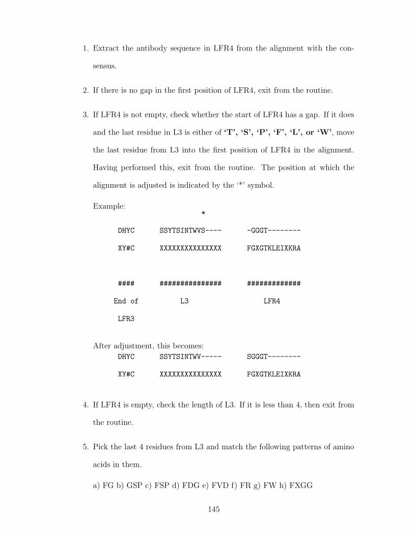
1. Extract the antibody sequence in LFR4 from the alignment with the con-
sensus.
2. If there is no gap in the first position of LFR4, exit from the routine.
3. If LFR4 is not empty, check whether the start of LFR4 has a gap. If it does
and the last residue in L3 is either of ‘T’, ‘S’, ‘P’, ‘F’, ‘L’, or ‘W’, move
the last residue from L3 into the first position of LFR4 in the alignment.
Having performed this, exit from the routine. The position at which the
alignment is adjusted is indicated by the ‘*’ symbol.
Example:*
DHYC SSYTSINTWVS---- -GGGT--------
XY#C XXXXXXXXXXXXXXX FGXGTKLEIXKRA
#### ############### #############
End of L3 LFR4
LFR3
After adjustment, this becomes:
DHYC SSYTSINTWV----- SGGGT--------
XY#C XXXXXXXXXXXXXXX FGXGTKLEIXKRA
4. If LFR4 is empty, check the length of L3. If it is less than 4, then exit from
the routine.
5. Pick the last 4 residues from L3 and match the following patterns of amino
acids in them.
a) FG b) GSP c) FSP d) FDG e) FVD f) FR g) FW h) FXGG
145

If one of these pattens is observed in the last 4 residues of L3, then move
these residues into LFR4 and exit from the routine.
Example:*
DYYC SSYTSISLTVLFG-- -------------
XY#C XXXXXXXXXXXXXXX FGXGTKLEIXKRA
#### ############### #############
End of L3 LFR4
LFR3
After adjustments, this becomes:
DYYC SSYTSISLTVL---- FG-----------
XY#C XXXXXXXXXXXXXXX FGXGTKLEIXKRA
6. Check the number of Glycines in the last 4 residues of L3. If it is less than
2, exit from the routine.
7. If there are at least 2 Glycines amongst the last 4 residues of L3, examine
the residue preceding the first Glycine. If it is one of ‘T’, ‘S’, ‘P’, ‘F’, ‘L’,
or ‘W’, then move the segment from the residue preceding the first glycine
to LFR4. Exit from the routine.
Example:
146

*
DYYC QTWGTGGG------- -------------
XY#C XXXXXXXXXXXXXXX FGXGTKLEIXKRA
#### ############### #############
End of L3 LFR4
LFR3
After adjustments, this becomes:
DYYC QTWG----------- TGGG---------
XY#C XXXXXXXXXXXXXXX FGXGTKLEIXKRA
#### ############### #############
End of L3 LFR4
LFR3
8. If the first residue among the last 4 residues in L3 is a Phenylalanine and the
third residue is Glycine, then move the last 4 residues from L3 into LFR4.
Having performed this, exit from the routine.
Example:
147

(a) Erroneous alignment in HFR3 end–H3–HFR4
(b) Correct alignment
Figure 4.8: Example of an error in the alignment for an equine heavy chain se-quence in the HFR3–H3–HFR4 region. The erroneous alignment (output from thenumbering program) is shown in (a) and the correct alignment is shown in (b).The beginning of H3 and HFR4 are marked by the ‘*’ symbol below the alignment.
*
DYHC GADHGSGSDFVGG-- -------------
XY#C XXXXXXXXXXXXXXX FGXGTKLEIXKRA
#### ############### #############
End of L3 LFR4
LFR3
After adjustments, this becomes:
DYHC GADHGSGSD------ FVGG--------
XY#C XXXXXXXXXXXXXXX FGXGTKLEIXKRA
148

4.1.8 Discussion
From preliminary analysis, it could be said that although the method was rea-
sonably accurate, there was no guarantee that the numbering output from the
program would be perfect owing to inherent limitations with using an alignment-
based approach. It also required a large set of relatively arbitrary rules to deal
with special cases. Unusual sequence features may lead to a wrong alignment
and therefore wrong numbering. An example of this is shown for an equine IgE
heavy chain sequence (Navarro et al., 1995) in the HFR3–H3-HFR4 region in Fig-
ure 4.8. The consensus sequence for CDR-H3 contains several X s to represent
the longest sequence that has been observed for this loop. However, this causes
a wrong alignment because the start of HFR4 is unusual. HFR4 usually starts
with a Tryptophan (W) whereas the start of HFR4 in this sequence is a Glycine
residue (G). It was therefore decided to implement a profile-based approach to ap-
ply numbering to antibody sequences in the hope that this would be less arbitrary
and more accurate.
4.2 A profile-based numbering method
This numbering algorithm uses profiles derived from the Kabat database to fix
anchor points in an antibody sequence. By fixing anchor points in the sequence,
it became possible to isolate the sequence of every region (framework region or
loop) and number each of them independently.
149

Chain type Sequence type Number of sequencesLight Complete 794Light Truncated 3044Heavy Complete 2641Heavy Truncated 1272
Table 4.5: Number of complete/truncated light and heavy chain sequences ex-tracted from the Kabat database.
4.2.1 Preparation of the dataset
Using KabatMan (Martin, 1996), sequences of antibodies were extracted from
the Kabat database (Johnson and Wu, 2001). For ease of benchmarking the
efficiency of the algorithm, the initial set of sequences were classified as being
truncated/complete light or heavy chain sequences. Any sequence with Kabat
annotations for the first and last residues of the variable region (L1, L109 in the
light chain and H1, H113 in the heavy chain) was regarded as being complete
and all other sequences were treated as truncated sequences. Table 4.5 gives the
number of complete and truncated light and heavy chain sequences extracted from
the Kabat database using KabatMan.
For structural analysis, a list of antibody structures was prepared by parsing the
XML file from SACS (Allcorn and Martin, 2002) and the structure files were
obtained from the PDB (Berman et al., 2000).
4.2.2 Creation of profile sets
The strategy adopted was to define a set of anchor points in the sequence and
to fill in the numbering based around these locations. The anchor points were
150

Anchor points for profileProfile name Light HeavyFR1 Start L1 - L6 H1 - H6FR1 End L18 - L23 H20 - H25FR2 Start L35 - L40 H36 - H41FR2 End L44 - L49 H44 - H49FR3 Start L57 - L62 H66 - H71FR3 End L83 - L88 H89 - H94FR4 Start L98 - L103 H103 - H108FR4 End L104 - L109 H108 - H113
Table 4.6: Kabat positions used in the profile definitions.
Chain type Sequence type Sequences that couldnot be numbered (%)
Light Complete 1/794 (0.12%)Light Truncated 44/3044 (1.44%)Heavy Complete 2630/2641 (99.58%)Heavy Truncated 1260/1272 (99.05%)
Table 4.7: Number of complete/truncated light and heavy chain sequences ex-tracted from the Kabat database that could not be numbered using just 3 profilesets (lambda, kappa, heavy).
chosen so that they would represent the start and end of every framework region.
For this I extracted the propensities of each of the 20 amino acids in the first and
last six positions of every framework region using KabatMan (Martin, 1996) and
a Perl script to analyse results. Each set of six residues was termed a profile and
a set of profiles representing the start and end of the four framework regions was
termed a profile set. Table 4.6 gives the list of Kabat positions that were used to
construct the profiles for the light and the heavy chain.
Initially, three profile sets were created, classified on the basis of chain– heavy
chain and lambda and kappa for the light chains. However, a significant number
of the sequences could not be numbered as anchor points for the start and end of
the framework regions could not be fixed in the correct order (See Table 4.7).
151

Classification Number ofprofiles
Human subgroups: Lambda class 6Human subgroups: Kappa class 4Human subgroups: Heavy chain 6Species: Lambda class 6Species: Kappa class 6Species: Heavy chain 4
Table 4.8: Classification scheme and number of profile sets.
Additional profile sets were then created to make each more specific. Table 4.8
lists 32 profiles that were created on the basis of the following criteria:
a) Human subgroup classes as identified by Kabat. From the 1994 version of
the Kabat database, sequences were divided into families based on amino acid
identity where members of a family differ by 12 amino acids or fewer (Deret et al.,
1995). This led to the creation of 16 human sub-group-specific profiles as shown
in Table 4.8.
b) Species of origin for the Lambda, Kappa and Heavy chain sequences. This
resulted in a further 16 non-human species-specific profiles as shown in Table 4.8.
As will be shown later, the development of more specific profiles significantly
improved the number of sequences that could be annotated using the numbering
program (see Table 4.11).
152

4.2.3 The numbering algorithm
To number a sequence, a sliding-window protocol is applied in which each window
consists of a set of six consecutive residues. The window is scored against a profile
before it is moved by a single residue to span the next set of 6-residues. The score
for a profile match is calculated as:
M = max(Sp,j); (j = 0..N − 6) (4.2)
Sp,j =5∑
i=0
log(Si+j) (4.3)
where M represents the score and Sp,j represents the score profile in the j’th
window of the sequence.
Once anchor points for the starts and ends of the framework regions have been
fixed, the sequence for every region (framework 1, loop 2, etc) is extracted and
numbered independently. However, it was noticed in several sequences that the
order of the anchor points was incorrect. For example, the anchor point of the
end of framework region 1 could appear after the anchor point for the start of
framework region 2. While detecting out-of-order misassignments is trivial, de-
tecting all misassignments of anchor points proved tedious requiring the design of
elaborate protocols to ensure error-free assignment.
153
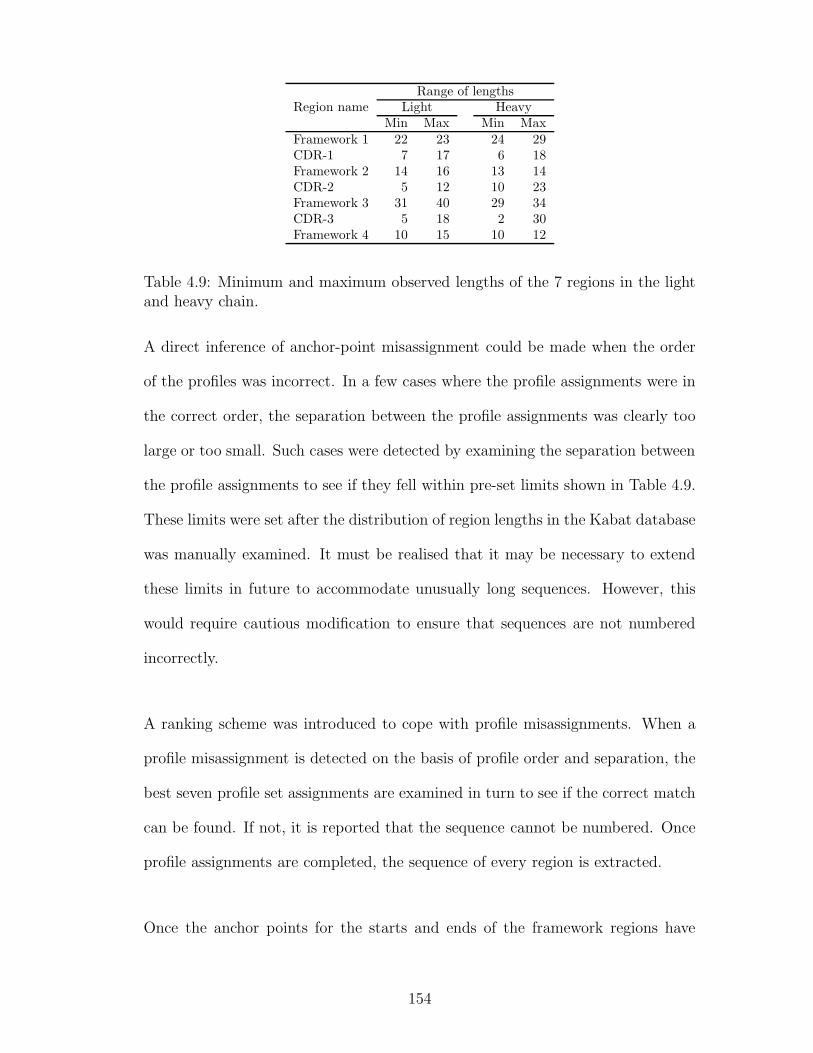
Range of lengthsRegion name Light Heavy
Min Max Min MaxFramework 1 22 23 24 29CDR-1 7 17 6 18Framework 2 14 16 13 14CDR-2 5 12 10 23Framework 3 31 40 29 34CDR-3 5 18 2 30Framework 4 10 15 10 12
Table 4.9: Minimum and maximum observed lengths of the 7 regions in the lightand heavy chain.
A direct inference of anchor-point misassignment could be made when the order
of the profiles was incorrect. In a few cases where the profile assignments were in
the correct order, the separation between the profile assignments was clearly too
large or too small. Such cases were detected by examining the separation between
the profile assignments to see if they fell within pre-set limits shown in Table 4.9.
These limits were set after the distribution of region lengths in the Kabat database
was manually examined. It must be realised that it may be necessary to extend
these limits in future to accommodate unusually long sequences. However, this
would require cautious modification to ensure that sequences are not numbered
incorrectly.
A ranking scheme was introduced to cope with profile misassignments. When a
profile misassignment is detected on the basis of profile order and separation, the
best seven profile set assignments are examined in turn to see if the correct match
can be found. If not, it is reported that the sequence cannot be numbered. Once
profile assignments are completed, the sequence of every region is extracted.
Once the anchor points for the starts and ends of the framework regions have
154

been fixed in the antibody sequence, the sequence of every individual region is
extracted. This is shown in Figure 4.9. The boundaries for every region are set
after the best profile assignments have been made and are known to be in the
correct order. In some cases, the input sequence contains a leader sequence at
the N-terminal end, or the constant region sequence at the C-terminal end. This
process excludes extraneous residues from the N-terminal or C-terminal end of the
antibody as they are not included in the alignment.
To ensure error-free assignment for the region boundaries (start and end of loop
and framework regions), a final check is performed by concatenating the sequences
in the individual regions and examining whether the concatenated sequence is a
substring of the original sequence. This check is particularly useful when the profile
representing the end of FR1 or the start of FR4 have been incorrectly assigned.
An example is shown in Figure 4.10.
Numbering is applied in every region based on one of the following rules:
1. Normal numbering where deletions are made before the position of inser-
tion – For example, the Kabat definition for region CDR-L2 is L50 to L56
giving it a standard length of 7 residues. A maximum length of 12 residues
(antibody Z84995 (Ignatovich et al., 1997)) and a minimum length of 6
residues (antibody Rer5 (Rast et al., 1994)) have been observed for this
region. The position of insertion according to the Kabat standard is L54
(L54A, L54B, L54C etc). Deletions are placed before the position of inser-
tion (L54). For example, in the case of a 5-residue CDR-L2, residues L53
and L54 are deleted. This is demonstrated in Figure 4.11.
155

Figure 4.9: Isolating the sequence of every region from the best profile assignments.Each profile represents the start or the end of a framework region.
156

Figure 4.10: Example showing the detection of errors through alignment with aconsensus sequence pattern. In this example, the profile assignment of heavy chainframework region 4 start is incorrect as framework 4 is truncated after the firstresidue (W). The alignment with the framework 4 consensus is shown in the finalbox.
157

L50 L51 L52 L53 L54 L55 L56G T T - - R T
(a) CDR-L2: GTTRT
L50 L51 L52 L53 L54 L55 L56G T T R - G T
(b) CDR-L2: GTTRGT
L50 L51 L52 L53 L54 L54A L55 L56E D S T T R G T
(c) CDR-L2: EDSTTRGT
Figure 4.11: Normal numbering in CDR-L2. The standard indel position is L54.Deletions are made before the position of insertion. The Kabat numbering isshown for varying lengths of CDR-L2. (a) 5 residues (GTTRT) (b) 6 residues(GTTRGT) (c) 8 residues (EDSTTRGT).
2. Reverse numbering where deletions are made after the position of insertion -
For example in CDR-L1, whose Kabat definition is L24 to L34, the standard
length is 11 residues. A maximum length of 17 residues and minimum length
of 7 residues have been observed in this region. Insertions are placed at
position L27 according to the Kabat standard. Deletions are placed after
the position of insertion (L27). For a 7-residue CDR-L1, residues L28, L29,
L30, and L31 are deleted. This is shown in Table 4.12.
3. Straight numbering where residues are numbered sequentially - In the heavy
chain framework region 4, residues are numbered sequentially as there are
no defined indels in this region. This is shown in Figure 4.13.
In some regions, the Kabat numbering does not impose a fixed site for indels. For
instance, in the heavy chain framework region 2 (HFR2) the deletion appears to be
placed at the most likely position based on sequence. In these cases, an alignment
158

L24 L25 L26 L27 L28 L29 L30 L31 L32 L33 L34S A S V - - - Y Y M Y
(a) CDR-L1: SASVYYMY (8 residues)
L24 L25 L26 L27 L28 L29 L30 L31 L32 L33 L34S A S - - S V Y Y M Y
(b) CDR-L1: SASSVYYMY (9 residues)
L24 L25 L26 L27 L28 L29 L30 L31 L32 L33 L34S A S S - S V Y Y M Y
(c) CDR-L1: SASSSVYYMY (10 residues)
Figure 4.12: Reverse numbering in CDR-L1. The standard Kabat indel positionis L27. Table shows the Kabat numbering where deletions are made after theposition of insertion (L27).
H103 H104 H105 H106 H107 H108 H109 H110 H111 H112 H113W G Q G T M V T V S -
(a) HFR4 - WGQGTMVTVS (10 residues)
L98 L99 L100 L101 L102 L103F G P G T K
L104 L105 L106 L106A L107 L108V T A L S Q
L109 L110 L111P - -
(b) LFR4 - FGPGTKVTALSQP (13 residues)
Figure 4.13: Straight numbering in HFR4. The sequence in the region is WGQGT-MVTVS and numbering is applied sequentially to residues.
159

Region Is alignment performed Is alignment used Numberingname for this region? in numbering? methodLFR1 Yes No 1
L1 No No 2LFR2 No No 1
L2 No No 1LFR3 No No 1
L3 No No 1LFR4 Yes No 3HFR1 Yes Yes 1
H1 No No 2HFR2 Yes Yes 3
H2 No No 2HFR3 No No 1
H3 No No 1HFR4 Yes No 3
Table 4.10: Regions in the light and heavy chain and methods that are used tonumber them.
is performed between the sequence in the region and a consensus pattern for that
region and numbering is applied based on the alignment. Table 4.10 summarises
the numbering methods used for the different regions in the Kabat numbering
scheme.
Figure 4.14 gives a flowchart of the numbering algorithm.
4.2.4 Benchmarking the numbering algorithm
In order to assess the performance of the profile-based numbering program, Ab-
Num, sequences of antibodies and their Kabat numbering were extracted from the
July 2000 release of the Kabat database. This was done using KabatMan and four
test datasets were prepared on the basis of chain type (light or heavy chain) and
nature of sequence (complete or truncated), as described in Section 4.2.1.
160

Startprogram
Read all sequences intomemory
Read all profilessets into memory
Read numbering filesinto memory
Read region informationinto memory
Any moresequences tobe numbered?
Y
Y
N
Start with arank of 1
For every profile segment in aprofile set, find the appropriately
ranked segment assignment in sequence
Calculate profile set score bysumming individual segment scores
Any profile segmentmisassignments?
Is Rank of lastassignment > 7
Y
Report that sequencecannot be numbered
Y
N
N
Translate the profilesegment assignments to
region boundaries
Extract sequencesof individual regions
Is concatenatedsequence asubstring of
originalsequence?N
Read next sequence
End Program
Number sequencein every regionindependently
Y
Align sequence in regionwith a consensus patternfor the region and adjust
region sequence if required
Concatenate sequencesof individual regions
IncreaseRank
Figure 4.14: Flowchart of the numbering program. Profile segment: First or thelast 6 residues in every framework region Region: Either means one of the sevenframework regions (LFR1, HFR3, etc) or a loop (CDR-L1, CDR-H2, CDR-L3,etc).
161

Figure 4.15 gives the algorithm for benchmarking the numbering program. All
sequences annotated in the Kabat database were numbered using AbNum. The
numbering of AbNum was compared with the Kabat numbering. The Kabat
database standard for numbering is very inconsistent in the range of L106–L111
in light chains and H100–H101 (including all residue insertions at H100: H100A,
H100B, H100C, etc.) in the heavy chain. For ease of comparison, residues in
these zones were excluded from examination. Sequences where the AbNum num-
bering matched the Kabat database numbering were regarded as being correctly
numbered. For the other cases where mismatches occurred, a random sample of
sequences was selected and manually examined to determine whether the error
was in the AbNum numbering, or in the Kabat database. These statistics were
then extrapolated to estimate the overall error percentages for the Kabat database
and AbNum as shown in Formulae 4.4 and 4.5:
Ek =ek × Nm
Ns
×100
NT
(4.4)
and
Ea =
(
Ua +(ea × Nm)
Ns
)
×100
NT
(4.5)
where Ek is the estimated percentage of errors in Kabat, Ea is the estimated
percentage of errors in AbNum, ek and ea are the number of errors identified in
Kabat and AbNum respectively in a sample of Ns sequences, Ua is the number
of sequences that AbNum was unable to number, Nm is the total number of mis-
matches between AbNum and Kabat and NT is the total number of sequences.
162

Chain type Status Total number Numbered Match Kabatof sequences
Light Complete 794 793 682Light Truncated 3044 3014 2688Heavy Complete 2641 2622 2416Heavy Truncated 1272 1245 793
Table 4.11: Number of sequences numbered by AbNum that match the Kabatdatabase annotations.
Table 4.11 gives the numbers of sequences that could be numbered by AbNum
and agreed with manual numbering in the Kabat database.
Table 4.12 shows the results of the benchmarking study. All discrepancies in the
AbNum numbering and Kabat database annotations were attributed to errors in
the manual Kabat numbering. Every sequence that could be numbered by AbNum
appears to have been numbered accurately.
4.3 Analysis of errors in the Kabat database
Since the manual examination of discrepancies between AbNum numbering and
the Kabat database numbering seemed to suggest that all were errors in the Kabat
database, I set out to examine the source of these errors. All sequences for which
the AbNum numbering differed from the Kabat numbering were isolated and a
region-wise distribution of these differences is shown in Table 4.13.
The following sections detail the nature of errors in each of these regions. All
definitions of regions described here are Kabat standard definitions.
163

N
CompleteLight chainSequences
Truncated Light chainSequences
CompleteHeavy chainSequences
TruncatedHeavy chainSequences
Split into 4 datasets
Kabatdatabase
Does Kabat databasenumbering match
AbNum numbering?
Consider AbNumnumbering and
Kabat numberingannotation as correct
Y
Calculate overall percentage ofKabat database annotation
error and AbNum error
Can sequencebe numberedusing AbNum
N
Y
Group allsequencess
with mismatches
Select a random sample of50 sequences
Manually examineseach sequence to
ascertain source of error
Categorize error asKabat annotation error
or AbNum error
Extrapolate to totalnumber of errors
Figure 4.15: Algorithm for benchmarking the numbering program.
164

Chain type Total number Not numbered Do not match Sample Error (%)of sequences Kabat size Kabat AbNum
Light chain complete 794 1 111 50 50/50 (14%) 0/50 (0.12%)Light chain truncated 3044 30 326 40 40/40 (10.7%) 0/40 (1%)Heavy chain complete 2641 19 206 50 50/50 (7.85%) 0/50 (0.72%)Heavy chain truncated 1272 27 452 39 39/39 (10.7%) 0/39 (2.12%)
Table 4.12: Benchmarking the performance of AbNum: comparison with the Kabat database annotations. The percentagesreported in the last two columns are estimated error percentages based on the sample set examined manually.
165

Chain type Total number of Number of errorsmismatches FR1 Loop1 FR2 Loop2 FR3 Loop3 FR4
Light chain complete 111 0 13 5 54 72 43 8Light chain truncated 326 5 71 7 112 73 187 49Heavy chain complete 206 70 4 13 71 47 92 10Heavy chain truncated 452 294 11 2 34 34 149 73
Table 4.13: Region-wise distribution of errors in the Kabat database.
166

Label L1 L2 L3 L4 L5 L6AbNum Q S A L T QKabat Q S A L T QLabel L7 L8 L9 L10 L11 L12AbNum P A S - V SKabat P A S V S GLabel L13 L14 L15 L16 L17 L18AbNum G S P G Q SKabat - S P G Q SLabel L19 L20 L21 L22 L23AbNum I T I S CKabat I T I S C
Figure 4.16: Kabat annotation error in LFR1. The 1-residue deletion is placed atL13 by Kabat although the Kabat standard imposes that it must instead be atL10.
Analysis of errors in the light chain
The Kabat standard assigns residues L1–L23 to LFR1. The usual length of LFR1
is 23 residues with a possible 1-residue deletion which according to the Kabat
standard is at position L10. However, as the LFR1 numbering for the protein B3
(Kalsi et al., 1996) in Figure 4.16 demonstrates the position of deletion in Kabat
is not consistent. Such errors have been corrected by AbNum as the position of
deletions has been enforced.
Similarly, incorrect numbering has been observed in CDR-L1. The Kabat standard
assigns residues L24-L34 to CDR-L1 with L27 as the indel position. A number of
incorrect assignments have been observed in this region such as the one shown in
Figure 4.17 for the protein SSbPB (Ivanovski et al., 1998). In the example, the one-
residue insertion must be placed at L27A (the second Serine in RASQSVSSSYLA)
whereas the Kabat database places the insertion at L27F with no L27A....L27E.
167

Label L24 L25 L26 L27 L27A L27BAbNum R A S Q S -Kabat R A S Q - -Label L27C L27D L27E L27F L28 L29AbNum - - - - V SKabat - - - S V SLabel L30 L31 L32 L33 L34AbNum S S Y L AKabat S S Y L A
Figure 4.17: Kabat annotation error in L1. The one-residue serine(RASQSVSSSYLA) has been assigned L27F by the Kabat database although itshould have been assigned L27A.
A different type of error has been observed to occur for the regions L1, LFR2, L2
and LFR3 as shown in Figure 4.18. The example shown is for the light chain of
the antibody SHLC5.1 (Hohman et al., 1992). The end of L1 has been incorrectly
annotated and the error can be seen to extend all the way up to LFR4. The
example in Figure 4.19 shows a similar case where the boundaries of L3 and LFR4
have been incorrectly assigned in the Kabat database.
Analysis of errors in the heavy chain
In the heavy chain too, similar errors with respect to incorrect assignment of
region boundaries have been observed. This is particularly clear in the case of
the H2–HFR3 region. The Kabat numbering for HFR3 is from H66 to H94 and
most sequences have a 3-residue insertion at H82 (H82A, H82B, H82C). However,
my analysis of mismatches between the Kabat and AbNum numbering led me
to discover a large number of discrepancies between the two annotations (nearly
30%). An example of this is shown in Table 4.20 which gives the Kabat database
numbering and the AbNum numbering for CDR-H2 and HFR3. This sequence
168

Original sequence
DPVLTQPGSISSSPGKTVTITCTMSGGTISSYWASWYWQKPDSAPVFVWSESDRMASGIPNRFAGSVDSSSNKMHLTITNVQSEDATDYYCAAAASRSPYRSIFGSGTKLNLGSPR
AbNum assignment
LFR1: DPVLTQPGSISSSPGKTVTITCL1: TMSGGTISSYWASLFR2: WYWQKPDSAPVFVWSL2: ESDRMASLFR3: GIPNRFAGSVDSSSNKMHLTITNVQSEDATDYYCL3: AAAASRSPYRSILFR4: FGSGTKLNLGSPR
Kabat database assignment
LFR1: DPVLTQPGSISSSPGKTVTITCL1: TMSGGTISSYWASWYLFR2: WQKPDSAPVFVWSESL2: DRMASGILFR3: PNRFAGSVDSSSNKMHLTITNVQSEDATDYYCL3: AAAASRSPYRSILFR4: FGSGTKLNLGSPR
Figure 4.18: Errors in the Kabat annotation in regions L1–LFR3. AbNum assignsthe boundaries of each of the regions correctly (marked in blue) whereas the Kabatannotation (which is wrong) is marked in red.
169

Original sequence
SYELTQPPSVSVPPGQTARITCSGDALPKKFAYWYQQKSGQAPVLVIYEDNKRPSEIPERFSGSSSGTMATLTISGAQVEDEGDYYCYSADINAKRVFGGGTKLTVLGQP
AbNum assignment
LFR1: SYELTQPPSVSVPPGQTARITCL1: SGDALPKKFAYLFR2: WYQQKSGQAPVLVIYL2: EDNKRPSLFR3: EIPERFSGSSSGTMATLTISGAQVEDEGDYYCL3: YSADINAKRVLFR4: FGGGTKLTVLGQP
Kabat database assignment
LFR1: SYELTQPPSVSVPPGQTARITCL1: SGDALPKKFAYLFR2: WYQQKSGQAPVLVIYL2: EDNKRPSLFR3: EIPERFSGSSSGTMATLTISGAQVEDEGDYYCL3: YSADINAKRVFGLFR4: GGTKLTVLGQPKA
Figure 4.19: Errors in the Kabat annotation in L3–LFR4. AbNum assigns theboundaries of each of the regions correctly (marked in blue) and the Kabat anno-tation (which is wrong) is marked in red.
170

Label H50 H51 H52 H52A H52B H53 H54 H55AbNum R F H S G R N PKabat R F H - - S G RLabel H56 H57 H58 H59 H60 H61 H62 H63AbNum P Q Y A S E A VKabat N P P Q Y A S ELabel H64 H65 H66 H67 H68 H69 H70 H71AbNum K G R V T A S TKabat A V K G R V T ALabel H72 H73 H74 H75 H76 H77 H78 H79AbNum D S S S C Y M QKabat S T D S S S C YLabel H80 H81 H82 H82A H82B H82C H83 H84AbNum M N S L - - K TKabat M Q M N S L K TLabel H85 H86 H87 H88 H89 H90 H91 H92AbNum E D T G I Y Y CKabat E D T G I Y Y CLabel H93 H94AbNum E DKabat E D
Figure 4.20: Kabat database error in the H2-HFR3 region of Axo1.
does not have the usual 3-residue insertion at H82 and this has been correctly
identified by AbNum. However, since the Kabat database annotations have largely
been manual and the 3-residue insert at H82 is very common, the sequence has
been incorrectly annotated as having residues at H82A-C whereas the insert should
have been at position H52 in CDR-H2.
171

4.4 Structural analysis: An alternate structure-
based numbering scheme to accommodate
indels in the framework regions
As described above, the two most widely used numbering schemes for antibodies
are the Kabat and the Chothia schemes. The Kabat numbering scheme (Kabat et
al., 1983) was based on sequence alignments and placed insertions where they oc-
curred in sequence. Chothia and co-workers (Chothia and Lesk, 1987; Al-Lazikani
et al., 1997) examined structures of antibodies and proposed a numbering scheme
correcting the positions of insertions at the structural level rather than at the
sequence level. However, only CDRs were included in this analysis and framework
regions were not examined.
A list of antibody structures was extracted from SACS (Allcorn and Martin, 2002).
Light chain and heavy chain sequences from 561 structures were extracted from
the SEQRES records of the PDB files. These were numbered using AbNum and
the numbering was patched into the PDB files using patchpdb (Dr. A. Martin,
unpublished). The sequence of every framework region was extracted and analysed
for deviations from the standard lengths described in Kabat (Wu and Kabat,
1970). Structures whose framework region lengths differed from the standard
were fitted using ProFit (Martin, ACR, http://www.bioinf.org.uk/software/
profit/). Where structures of variable regions were not available, four or five
structures were chosen and fitted together to see if certain positions in the region
are more flexible than others and therefore likely to accommodate indels.
172

Region Kabat definition Length range Kabat indel Structural StructuralName (Standard length) Min - Max position ins. pos. del. pos.LFR1 L1 - L23 (23) 22 - 23 L10 - L10LFR2 L35 - L49 (15) 14 - 16 - L40 L41LFR3 L57 - L88 (32) 31 - 40 L66 L68 L68LFR4 L98 - L110 (12) 12 - 13 L106 L107 -HFR1 H1 - H30 (30) 29 - 34 H6 H8 H8HFR2 H36 - H49 (14) 13 - 14 - - H42HFR3 H66 - H94 (29) 30 - 34 H82 H72 -
Table 4.14: Table comparing the Kabat indels with the structurally correctedindels.
Table 4.14 compares the results of this analysis with the Kabat standards for the
positions of insertions and deletions in the framework regions. For LFR1 (Kabat
definition L1 to L23) which has a standard length of 23 residues, a structure with
22 residues (PDB Code 2vit (Fleury et al., 1998)) was found. 2vit also has an
LFR4 (Kabat definition L98 to L110) length of 13 residues compared with the
standard length of 12 residues. I fitted the LFR1 and LFR4 regions of 2vit to
that of 12e8 (Trakhanov et al., 1999) which has standard lengths in these regions.
For the remaining regions however, no structures with unusual framework region
lengths exist.
The fitted structures of light and heavy chain framework regions are shown in Fig-
ures 4.21 and 4.22 respectively indicating the Kabat indel sites and my proposed
structurally correct sites.
The case of HFR3 is particularly interesting. The Kabat definition for HFR3 is
from H66 to H94, a standard length of 29 residues. In most heavy chains however,
there is a 3-residue insertion in HFR3 which Kabat designates as being at H82
(H82A, H82B, H82C); see Figure 4.23a. There are a small number of sequences
173

that do not contain this insertion, but because this situation is rare, the majority
of these are erroneously annotated in Kabat as containing the 3-residue insertion
in HFR3 whereas the residues should be inserted in CDR-H2 at position H52
(Figure 4.23b). In total, 74 sequences in Kabat were identified where the end of
the CDR-H2 and the start of heavy chain framework region 3 have been annotated
incorrectly.
Further analysis of HFR3 indicates that position H82 is unlikely to accommodate
insertions. A pairwise sequence alignment between antibodies axo1 (Patel and
Hsu, 1997) and mab113 (Mantovani et al., 1993) as shown in Figure 4.24 suggests
that H72 is the likely position of the 3-residue insertion. Figure 4.25 shows the
spacefilled representation of the Fv region of an antibody. Residues that would be
numbered H72 and H82 are indicated and it can be seen that H82A-C are relatively
buried while H72A-C are on the surface making it more likely that these residues
would be deleted. This is further corroborated by the work of Annemarie Honegger
(Honegger and Pluckthun, 2001) who analysed the sequences and structures of
light chain and heavy chain variable regions of antibodies and suggested that the
heavy chain has a 2-residue insertion with respect to the light chain at position
H72.
4.5 Conclusions
In this chapter, a new method that uses profiles to apply numbering schemes to
antibody sequences has been described. This approach successfully numbers the
174

‘problem’ sequence described in Section 4.1.8. The analysis of manual annotations
in the Kabat database shows that there is a high percentage of errors. Based on
structural analysis of insertions and deletions in the framework regions of anti-
bodies, I have extended the Chothia numbering scheme to correct the positions of
insertions and deletions in the framework regions.
175

(a) LFR1 (b) LFR2
(c) LFR3 (d) LFR4
Figure 4.21: Rigid body superposition of light chain framework regions. Colourcodes are: red - kabat indel position, green - structurally correct position of inser-tion, pink - structurally correct position of deletion.
176

(a) HFR1 (b) HFR2 (c) HFR3
Figure 4.22: Rigid body superposition of heavy chain framework regions. Colourcodes are: red - kabat indel position, green - structurally correct position of inser-tion, pink - structurally correct position of deletion.
(a) Standard
(b) Correct
Figure 4.23: Numbering in H2-HFR3 (a) The standard numbering for H2-HFR3in the Kabat database annotations (b) The correct numbering when the 3-residueinsertion at H82 are not present.
177

axo1 QIVLTQSGSEVKKPGESMQLKCTVTGFNVNSYWMHWVRQAPGmab113 QVQLVQSGAEVKRPGAPVKVSCKASGYTFTDYYMHWVQQAPG
...CDR−H2−> <−HFR3...axo1 KGLEWVLRFHSGRNPPQYASEAVKG RVTASTDS−−SSCmab113 QGLEWMGRINPNTGGTN−SAQKFQG RVTMTRDTSISTA 65 6789012abc345
..HFR3−>axo1 YMQMNSLKTEDTGIYYCARmab113 YMELSNLRSDDTAMYSCAR 6789012345678901234
(a) Alignment if position of insertion is H72
axo1 QIVLTQSGSEVKKPGESMQLKCTVTGFNVNSYWMHWVRQAPGmab113 QVQLVQSGAEVKRPGAPVKVSCKASGYTFTDYYMHWVQQAPG
...CDR−H2−> <−HFR3...axo1 KGLEWVLRFHSGRNPPQYASEAVKG RVTASTDSSSCYMmab113 QGLEWMGRINPNTGGTN−SAQKFQG RVTMTRDTSISTA 65 6789012345678
..HFR3−>axo1 QMNSL−−KTEDTGIYYCARmab113 YMELSNLRSDDTAMYSCAR 9012abc345678901234
(b) Alignment if position of insertion is H82
Figure 4.24: Sequence alignment between antibodies Axo1 and mab113.
178

Figure 4.25: Spacefill representation of the variable domain of an antibody.The colour codes are: light chain - blue gray, heavy chain - pink, HFR3 - yel-low and highlighted by the white borders. The residues coloured in blue andgreen are H72A-C (if insert position is H72) and H82A-C (if insert positionis H82) respectively. This diagram was prepared using QTree (Martin, ACR,http://www.bioinf.org.uk/software/qtree/).
179

Chapter 5
Predicting the VH/VL interface
angle from interface residues
The variability of antibodies is encoded in the Fv region which consists of two
protein domains. Interactions between the light and the heavy chain contribute
significantly to the stability of the variable fragment (Fv). The VH/VL interface
between the light chain and heavy chain has been shown to affect the binding
kinetics of a peptide (Chatellier et al., 1996). The framework region at the VH/VL
interface consists of two β-sheets (Poljak et al., 1973), the structures of which
are conserved across Fab and light chain dimers (Chothia et al., 1985; Novotny
and Haber, 1985). However, the contribution of residues in the framework re-
gions to interactions with the antigen remains poorly understood. It has been
demonstrated that modification of residues distant from the antigen binding site
of the antibody has a small yet significant effect on the binding affinity with the
180

antigen (Chatellier et al., 1996; Roguska et al., 1996). For example, Adair and co-
workers have demonstrated that modification of residue H23 significantly affects
binding of the antibody with the antigen (Adair et al., 1999). While this may be
an impediment for predicting the affinity of engineered antibodies, it must also
be emphasised that interactions at the VH/VL interface are crucial to maintaining
stability of the Fab. Understanding the influence of residues in the VH/VL interface
on the packing angle between the two domains would help design antibodies with
a definable binding site topography.
In this chapter, I present an analysis of the distribution of the VH/VL packing angle
and a method to predict the interface angle from the nature of interface residues
is described. A set of conserved residues in the framework regions of VL and VH
were chosen and the interface angle was defined as the torsion angle between these
points. The main applications of trying to predict packing angle from interface
residues are in modelling studies of antibodies and in humanization protocols.
The packing angle between the variable chains of antibodies has previously not
been considered when modelling variable chains of antibodies (Martin et al.,
1991; Martin et al., 1989; Whitelegg and Rees, 2000). Knowing the packing angle
prior to modelling the variable region light and heavy chain may help in choosing
more appropriate template structures upon which models may be based. This
work also helps in identifying key residues that influence the packing angle and
therefore, are instrumental in determining the topography of the paratope. The
process of humanization involves grafting of murine CDRs onto human framework
regions (Jones et al., 1986). Further modification of residues flanking the CDRs is
usually required to restore the binding affinity of the mouse antibody (Riechmann
et al., 1988). This could be extended by modifying residues at the VH/VL interface
181

in the humanized antibody to their murine counterparts so that the topography
of the paratope would be preserved.
5.1 Preparation of the dataset
A list of Fv and Fab structures was extracted from the SACS (Allcorn and Mar-
tin, 2002) XML file. This yielded a set of 561 antibody structures including 6
anti-idiotype antibodies (PDB Codes: 1cic, 1dvf, 1iai, 1pg7, 1qfw, and 2dtg).
Anti-idiotype antibodies are antibodies derived against epitopes present in other
antibodies. As every anti-idotypic antibody structure consists of two antibodies,
all anti-idiotype antibody structures were split into two and the final dataset con-
sisted of 567 antibody structures. This set comprised 314 structures for which
the sequences of the light chain and heavy chain were distinct. Conformational
changes in the antibody CDRs upon binding with the antigen have been estab-
lished in several studies (Colman et al., 1987; Bhat et al., 1990; Herron et al.,
1991; Rini et al., 1992; Wilson and Stanfield, 1994; Mylvaganam et al., 1998).
The idea behind allowing redundancy in the dataset is that it allows for vari-
ability in a given structure. Structural fitting of antibodies was performed using
ProFit (http://www.bioinf.org.uk/software/profit/) which implements the
McLachlan algorithm (McLachlan, 1982). The AbNum program described in the
previous chapter was used to apply Chothia numbering to the structures of anti-
bodies.
Programs for analysis were written in C and PERL. All graphs were created us-
182

ing GNUPLOT and GRACE (http://plasma-gate.weizmann.ac.il/Grace/).
The program ssearch33 from the FASTA package (Pearson and Lipman, 1988)
was used in the calculation of Z-scores for chain assignment. The Stuggart Neu-
ral Network Simulator (SNNS) (http://www-ra.informatik.uni-tuebingen.
de/SNNS/) was used to make associations between packing angle and interface
residues. The GRASS library (Team, 2006) was used for calculation of Eigen
vectors and values. The Sun gridengine was used to distribute jobs across a grid
consisting of the C3 and the Queen. The C3 is a farm consisting of 96 IBM series
335 nodes and the Queen is a farm consisting of 30 nodes with each node having
2 dual-core AMD Opteron processors.
The ‘interface residues’ are defined as Chothia-numbered interface positions for
which there is a change in accessibility as a result of VH/VL interaction. As a
first step, sequences of the light and heavy chain were extracted from PDB files
of the antibodies. The Chothia numbering scheme (Chothia and Lesk, 1987; Al-
Lazikani et al., 1997) was applied to all the sequences using AbNum. In the case
of Fabs, only the variable region was considered for further analysis. The Chothia
numbered variable region sequences were patched back into the PDB files to yield
567 numbered Fv region structures.
Once the structure files were prepared with the Chothia numbering applied to
them, the accessibility of all residues in the light and heavy chains was calculated.
Simon Hubbard’s naccess program that implements the algorithm described by Lee
and Richards (1971) was used for the calculation of accessibility. The accessibility
of all residues in the VH/VL complex and in the individual chains was calculated.
Those residues which sustained any change in the accessible surface area were
183

regarded as being interface residues.
5.2 Calculation of the packing angle
The packing angle was defined as the torsion angle at the VH/VL interface. The
steps involved in the calculation of the packing angle are as described below:
1. Identify a set of residues SL and SH that are structurally conserved in the
light and heavy chain respectively.
2. Extract the Cα coordinates for the residues in SL and SH.
3. Find the centroid for each set (CL and CH).
4. For each set, compute the best-fit line passing through the centroid.
5. Identify one point on each line PL and PH on the same side relative to the
respective centroid.
6. Calculate the packing angle as the torsion angle between the points PL, CL,
CH, and PH.
Five antibody light and heavy chains were fitted together on all residues in the
variable region using ProFit to identify conserved residues at the VH/VL interface.
The backbone representations of the fitted structures are shown in Figures 5.2
and 5.3 respectively. The regions coloured in blue correspond to residues that are
highly conserved across antibody structures. These are L35-L38, L85-L88 in
184

Start
Perform rigid-bodysuperposition for a setlight and heavy chain
variable domains
Identify a set of structurallyconserved positions in each
chain - SL (light chain)and SH (heavy chain)
Extract CA coordinates ofthe residues in SL and SH
Find the centroidfor each set
For each set, computea best-fit line passingthrough the centroid
Identify one point on eachline on the same side relative
to the respective centroid
Calculate packing angle asthe torsion angle between
these points
Stop
Figure 5.1: Algorithm to calculate the packing angle at the VH/VL interface.
185

Figure 5.2: Rigid body superposition of the Cα atoms in five structures of thelight chain variable region. The structures used were: 12e8, 15c8, 1a0q, 1a3l,1a3r.
186

Figure 5.3: Rigid body superposition of the Cα atoms in five structures of theheavy chain variable region. The structures used were: : 1oax, 1yec, 1yef,2ddq, 8fab.
187

Figure 5.4: The beta strands at the VH/VL interface, best-fit lines, and packingangle.
188

the light chain and H36-H39, H89-H92 in the heavy chain. These positions
form part of a beta-sheet which is at the core of the interface and outside the
hyper-variable loops. Figure 5.4 shows the beta sheets, the best-fit lines drawn
through them, and the packing angle.
The next step was to calculate a best-fit line for the points in SL and SH. Only
the coordinates of the Cα atoms were used to compute the best-fit line. The
method employed was Principle Component Analysis (PCA) and the calculations
were performed according to the algorithm shown in Figure 5.5.
After calculation of the packing angle across the 567 structures in the dataset, their
frequency distribution was plotted and this is shown in Figure 5.6. The packing
angle varies quite considerably across different structures. The smallest and largest
packing angles observed were 300 and 600 in the structures 1FL3 (Simeonov et al.,
2000) and 1BGX (Murali et al., 1998) respectively. The extreme packing angles
are shown in Figure 5.7.
5.3 Identifying interface residues
Interface residues for the 567 structures were defined as described in Section 5.1.
Owing to the variability in the VH/VL packing angle, the interface residues in
any given structure will be a subset of the total set. A total of 124 positions
(63 light chain and 61 heavy chain positions) were identified as contributing to
the interface in at least one of 567 structures. Figure 5.8 shows the plot of the
189

1. For points in a set (SL or SH ) calculate centroid C (CL or CH).
2. Compute the covariance matrix. The pseudocode for this is given below:
For i=0 to 3(number of dimensions)
Do
For j=0 to 3(number of dimensions)
Do
Total = 0
For start=0 to 4 (number of points in set SL or SH)
Do
Total+=( x[start][i] - C[i] ) *
( x[start][j] - C[j] )
Done /* End of loop For start=0 to 4 */
Covariance(i,j) = Total/(number of points in SL or SH)
Done /* End of For j=0 to 3 */
Done /* End of For i=0 to 3 */
3. Perform an eigen decomposition for the covariance matrix. Calculate eigenvalues and eigen vectors.
4. The eigen vector represented by the largest eigen value is the best-fit linewhen it passes through the centroid.
Figure 5.5: Algorithm used in the calculation of the best-fit line for the light andheavy chain variable regions.
190

30 35 40 45 50 55 60Packing angle
0
10
20
30
40
50
Freq
uenc
y
Figure 5.6: Frequency distribution of the packing angle.
191

(a) 1FL3
(b) 1BGX
Figure 5.7: Extreme packing angles in (a) 1FL3 - 300 (b) 1BGX - 600.
192

0 10 20 30 40 50 60 70 80 90 100 110Light chain position
0
100
200
300
400
500
600
Freq
uenc
y
Frequency distribution at interface: light chain
(a) Light chain
0 10 20 30 40 50 60 70 80 90 100 110Heavy chain position
0
100
200
300
400
500
600
Freq
uenc
y
Frequency distribution at interface: heavy chain
(b) Heavy chain
Figure 5.8: Frequency distribution of interface residues in (a) The Light chain and(b) Heavy chain.
193

frequency distribution of interface residues in the light chain and heavy chain.
5.4 Predicting packing angle from interface residues
It was decided to use a neural network to predict the packing angle from the
interface residues. Amino acids representing the interface residues in different
structures were used as input for the neural network and the output was the
packing angle. The process of training a network involves supplying a set of input
patterns and the output (the result to be predicted) values to help the neural
network ‘learn’ from the data. Once the network has passed the learning phase, it
is supplied with inputs for which it is expected to make predictions of the output
values. The predictions of the neural network are compared with the actual values
and the performance of the neural network is assessed. Here, a five-fold cross
validation was performed. In this procedure, the neural network is trained on 45
of the total data available and the quality of its training is evaluated by assessing
its predictions on the remaining 15
of the data. This is repeated on each slice of
the data and the overall performance is averaged over the five folds.
The input is fed to the neural network in the form of numbers that represent
the amino acids at the interface. A common method of doing this is using a
20-dimensional binary vector representing the 20 amino acids or values from a
similarity matrix. The binary vector contains nineteen 0s and one 1 to indicate
a specific amino acid or values from a similarity matrix. The input layer size is
calculated as:
194
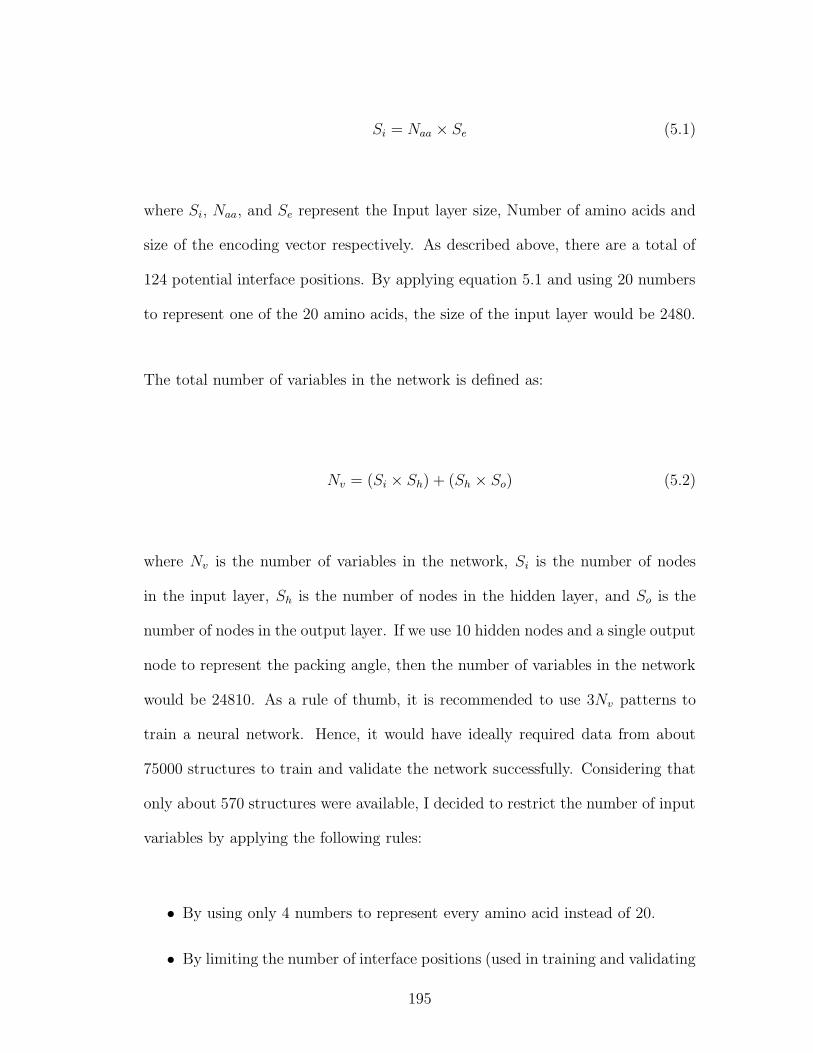
Si = Naa × Se (5.1)
where Si, Naa, and Se represent the Input layer size, Number of amino acids and
size of the encoding vector respectively. As described above, there are a total of
124 potential interface positions. By applying equation 5.1 and using 20 numbers
to represent one of the 20 amino acids, the size of the input layer would be 2480.
The total number of variables in the network is defined as:
Nv = (Si × Sh) + (Sh × So) (5.2)
where Nv is the number of variables in the network, Si is the number of nodes
in the input layer, Sh is the number of nodes in the hidden layer, and So is the
number of nodes in the output layer. If we use 10 hidden nodes and a single output
node to represent the packing angle, then the number of variables in the network
would be 24810. As a rule of thumb, it is recommended to use 3Nv patterns to
train a neural network. Hence, it would have ideally required data from about
75000 structures to train and validate the network successfully. Considering that
only about 570 structures were available, I decided to restrict the number of input
variables by applying the following rules:
• By using only 4 numbers to represent every amino acid instead of 20.
• By limiting the number of interface positions (used in training and validating
195

the neural network) to 20 instead of 124.
The four numbers used to represent every amino acid were chosen on the basis of
the following physical properties:
1. Size of the amino acid, in terms of the number of atoms in the side-chain.
2. Size of the amino acid expressed as the shortest path from the Cα atom to
the atom farthest away from it, i.e. the length of the sidechain.
3. Hydrophobicity
4. Charge
Table 5.1 lists the numbers used to represent the 20 different amino acids. The hy-
drophobicity scales used were taken from the consensus values reported by Eisen-
berg et al. (1982). I decided to use a 4-dimensional encoding vector with 20
interface residues chosen as being most likely to influence the packing angle. By
doing this, the input layer size was reduced to 80 nodes.
Initially, a manual selection of 20 interface residues most likely to influence the
packing angle made using the following sets of criteria:
Method I Highest change in Accessible Surface Area (ASA) in any one structure.
Method II Highest average change in ASA
Method III Most frequently occurring positions with highest change in ASA
196

Amino acid Size Size Hydrophobicity ChargeNS SP
Alanine (A) 1 1 0.250 0Valine (V) 3 2 0.540 0Leucine (L) 4 3 0.530 0Isoleucine (I) 4 3 0.730 0Proline (P) 3 4 -0.07 0Methionine (M) 4 4 0.26 0Phenylalanine (F) 7 5 0.610 0Tryptophan (W) 10 6 0.370 0Glycine (G) 0 0 0.160 0Serine (S) 2 2 -0.26 0Threonine (T) 3 2 -0.18 0Cysteine (C) 2 2 0.04 0Asparagine (N) 4 3 -0.64 0Glutamine 5 4 -0.69 0Tyrosine (Y) 8 6 0.02 0Aspartate (D) 4 3 -0.72 -1Glutamate (E) 5 4 -0.62 -1Lysine (K) 5 5 -1.1 1Arginine (R) 7 6 -1.8 1Histidine (H) 6 4 -0.4 0.5
Table 5.1: Amino acid properties for size, hydrophobicity and charge. NS: numberof side chain atoms in the amino acid; SP: shortest path to the atom farthest awayfrom the Cα atom of the residue. 0.5 was chosen as the charge for Histidine torepresent the fact that it can exist in both charged and uncharged states.
197

Input layer
Nodes representing residues at interface positions
Nodes in thehidden layer -10, 20, or 30
Hidden layer
Output node representingInterface angle
Output layer
Figure 5.9: Architecture of a fully connected network. Not shown in the figure arethe connections between every pair of nodes in the input layer and hidden layerand between nodes in the hidden and output layer.
Method IV Most frequently occurring positions with highest average change in
ASA
The top 10 positions in each chain (light and heavy) were taken and a 5-fold cross
validation was performed. Table 5.2 lists the interface positions that were manu-
ally selected. A fully connected artificial neural network was constructed with the
architecture shown in Figure 5.9. Using the Stuggart Neural Network Simulator
(SNNS) the neural network parameters: learning function, update function, ini-
tialisation function, shuffling and number of cycles were varied and the following
values were found to be most optimal for the problem:
1. Number of cycles of training - 150
198

Method Interface positions
Method I
L34, L36, L44, L46, L50L87, L89, L91, L96, L98
H35, H47, H91, H100B, H100CH100D, H100I, H100G, H100M, H103
Method II
L34, L36, L43, L44, L46L86, L87, L89, L91, L98
H35, H47, H91, H100B, H100CH100D, H100G, H100I, H100M, H103
Method III
L32, L34, L36, L44, L46L50, L87, L91, L96, L98
H45, H47, H50, H91, H99H100, H100A, H100B, H101, H103
Method IV
L34, L36, L38, L43, L44L46, L87, L91, L96, L98
H39, H45, H47, H91, H99H100, H100A, H100B, H101, H103
Table 5.2: Manually chosen interface positions based on methods (I) Highestchange in ASA, (II) Highest average change in ASA, (III) Most frequently oc-curring positions with highest change in ASA, and (IV) Most frequently occurringpositions with highest average change in ASA.
2. Training until sum-of-squares error (SSE) becomes <= 1.5
3. Init function - Randomise weights
4. Learning function - RProp
5. Update function - Topological order
6. Pruning function - Magnitude pruning.
7. Shuffling - TRUE
8. Number of hidden nodes - 10.
A neural network consists of a set of ‘perceptrons’ which generate values between
0 and 1 using a sigmoid function applied to a weighted sum of the inputs:
199

Method Average Pearson’s coefficientover 5 folds
I 0.32II 0.38III 0.40IV 0.30
Table 5.3: Results of a 5-fold evaluation over interface positions chosen manuallyusing the four methods described in the text. The correlation coefficient reportedhas been averaged over the 5 folds.
O = f(N∑
i=1
Wixi) (5.3)
where O is the output of the perceptron, f() is the sigmoid transfer function, xi
is an input, Wi is an weight and N is the number of inputs. I therefore decided
to represent all output values (packing angles) by a value between 0 and 1. The
scaling of packing angles was done according to:
θf =θ − θmin
θmax − θmin(5.4)
where θf is the interface angle fraction, θ is the interface angle, θmax is the maxi-
mum observed interface angle, and θmin is the minimum observed interface angle.
From manual examination, it appeared that shuffling the training data (item 7
in the list of optimal SNNS parameters shown above) while training the neural
network had a positive effect. However, this could not be used when training and
validating the neural network through scripts as it appears that this feature is
only supported by the graphical interface to SNNS.
200

To evaluate the performance of the neural network, the Pearson’s correlation co-
efficient (r) was initially used to compare the output of the neural network and
the actual scaled packing angle (between 0 and 1):
rxy =
n∑
i=1(xi − x)(yi − y)
(n − 1)sxsy
(5.5)
where rxy is the Pearson’s correlation coefficient between two variables x and y,
n is the number of data points, xi and yi are the individual values of variables x
and y, and sx and sy are the standard deviations of the two distributions x and y.
Table 5.3 shows the result of training and validating the neural network based on
the manual selection of interface positions. None of the methods to select interface
residues manually worked particularly well as the Pearson’s correlation coefficient
for all methods was low. However, from manual examination of correlation coef-
ficients over single folds, correlation coefficients as high as 0.6 had been observed.
I therefore decided to have the computer sample sets of interface positions to find
the combination that would be most predictive of the packing angle.
5.5 Using a genetic algorithm to sample the interface-
residue space
The use of a genetic algorithm (GA) for feature selection (i.e. to sample sets
of interface residues and pick the most optimal set) appeared to be a potential
201

Figure 5.10: An individual to represent 10 interface positions. From the stringshown, those alleles with a 1 imply the inclusion of the residue at the respectiveinterface position for training and validation of the neural network.
solution to the problem of low scores of manually selected interface positions.
The overall method of the genetic algorithm developed to sample the space of
interface residues is described below:
1. Create a random population of individuals where each individual represents
a set of interface positions, each allele being a 1 or 0 to indicate whether a
given interface position is included in training the neural net.
2. Evaluate the quality of each individual by training and validating the neural
network over 5 folds (5-fold cross-validation)
3. Create a new population of individuals by crossover of high-scoring individ-
uals.
4. Repeat the above steps for as many generations as required.
202

Figure 5.11: Crossover of two high-scoring individuals A and B
The first step involves the creation of a random population of individuals. Every
individual is a string whose length is the number of interface positions. It consists
of a set of 0s and 1s (alleles) and represents a selection of interface positions to be
used to train and validate a neural network. This is demonstrated in Figure 5.10.
The quality of every individual is assessed by training the neural network and
averaging the Pearson’s correlation coefficient over 5 folds. Initially, a random
population of individuals is created and the quality of every individual is assessed.
A new population of individuals is then generated by selective crossover of high
scoring individuals which is shown in Figure 5.11. Newly created offspring individ-
uals are subject to random mutations at a rate referred to as the mutation rate (µ).
In this work, unless otherwise specified, a default mutation rate of 0.0001 has been
used for Rank-based selection (See Section 5.6). Once the random mutations have
been effected, the offspring individuals become children. These children become
203

the parents for the next generation. They are scored by training and validating
the neural network and further generations of the genetic algorithm progress in
the same way. These steps are repeated until the required number of generations
have been completed or the population has converged.
5.6 Methods of selection
In the process of creating offspring through crossover, a bias is made towards the
selection of parents that have high scores. There are many selection methods for
choosing the parents and in this project, I primarily used Roulette-wheel based
selection and Rank-based selection. These selection strategies have already been
addressed in Chapter 2.
Generation Best Pearson’s r
Rank Roulette-wheel
1 0.4964 0.4980
2 0.5039 0.5082
3 0.5039 0.5082
4 0.5007 0.5082
5 0.5039 0.5082
6 0.5167 0.5082
7 0.5159 0.5082
8 0.5122 0.5082
9 0.5581 0.5054
continued on next page
204

continued from previous page
Generation Best Pearson’s r
Rank Roulette-wheel
10 0.5266 0.5082
11 0.5271 0.5082
12 0.5581 0.5054
13 0.5581 0.5054
14 0.5318 0.5082
15 0.5503 0.5082
16 0.5703 0.5082
17 0.5703 0.5054
18 0.5586 0.5082
19 0.5703 0.5082
20 0.5572 0.5082
21 0.5703 0.5054
22 0.5703 0.5082
23 0.5703 0.5082
24 0.5703 0.5082
25 0.5703 0.5082
26 0.5626 0.5082
27 0.5910 0.5082
28 0.5910 0.5082
29 0.5910 0.5054
30 0.5829 0.5082
continued on next page
205

continued from previous page
Generation Best Pearson’s r
Rank Roulette-wheel
31 0.5870 0.5082
32 0.5910 0.5082
33 0.5910 0.5054
34 0.6006 0.5082
35 0.5910 0.5082
36 0.5946 0.5082
37 0.6149 0.5082
38 0.6006 0.5054
39 0.5910 0.5054
40 0.5910 0.5082
Table 5.4: Comparing Roulette-wheel and Rank-based
selection methods. The table shows the best Pearson’s r
calculated over 40 generations of a GA run.
The effectiveness of a selection procedure is largely assessed by the ability of the
procedure to keep the population diverse (i.e. avoid local minima) and yet achieve
convergence in a reasonable time span. To decide on the method best suited for
the current problem, I performed test runs of the GA on small populations of
individuals for short durations using both Rank-based and Roulette-wheel based
selection methods. Results from a sample run are summarised in Table 5.4. From
the table, it can be seen that the initial scores were nearly equal (0.496 in Rank and
206

0.498 in Roulette-wheel based selection). However, there is a steady increase in
best score for Rank-based selection whereas the best score remains largely static
for Roulette-wheel based selection. It was therefore decided to use Rank-based
selection for future runs of the GA.
5.7 Problems: Redundancy in individual popu-
lation and intelligent selection
A problem with Rank-based selection that became apparent after a few tens of
generations of the GA was that the population of individuals was becoming de-
creasingly diverse. Figure 5.12a shows a graph of a GA run where Rank selection,
together with a mutation rate of 0.0001 were used. The score of the best individ-
ual at the end of 50 generations was 0.638. This could have meant either a) The
genetic algorithm was converging to a globally optimal solution, or b) The GA
was getting stuck in a local minimum problem.
It was assumed that the GA was getting stuck in a local minimum and, as will
become clear from the following sections, this was indeed the case. I developed an
alternative method to alter the mutation rate dynamically during crossover.
In Rank-based selection, the creation of new child individuals is done by bias-
ing selection towards high-scoring parents. A crossover point is chosen randomly
within the parents and the two parts of the parents are combined to yield offspring
(Figure 5.11). When the number of redundant individuals in the population in-
207

0 10 20 30 40 50
Generation
0
1000
2000
3000
4000
5000
Num
ber o
f red
unda
nt in
divi
dual
sRank-based selection
(a)
0 10 20 30 40 50 60
Generation
0
200
400
600
800
1000
Num
ber o
f red
unda
nt in
divi
dual
s
Rank-based selection
(b)
Figure 5.12: Redundancy of individuals in a GA run using Rank-based selectionwith (a) 5000 individuals and µ=0.0001 (b) 1000 individuals and µ=0.001.
208

creases, the chances of choosing two identical individuals randomly for crossover
also increases. Crossover of identical individuals would clearly yield a child iden-
tical to the parents. Since the mutation rate applied to the offspring individual
is very low (0.0001), the final offspring are likely to be unchanged. However, a
higher mutation rate (µ=0.001) did not help curb the exponential rise in the num-
ber of redundant individuals with the passage of every generation. Figure 5.12b
shows that the population of individuals quickly saturates and by the end of 60
generations, nearly the entire population of individuals is redundant.
As a solution to the problem of individual redundancy, I developed a combina-
torial approach. Parent individuals are selected using Rank-based selection, but
a modification to the strategy of using a standard mutation rate was made so
that the mutation rate was varied dynamically, depending on how similar the par-
ents selected for crossover are. The method, which I term Intelligent selection, is
described below:
1. For every child individual to be created, select 2 parents P1 and P2 based
on Rank Based Selection.
2. Choose a cross over point and splice P1 and P2 to create a child Oi.
3. Calculate the degree of similarity S(P1,P2) between the parents P1 and P2 as
given by:
S(P1,P2) =C(P1,P2)
N(P1,P2)(5.6)
where C(P1,P2) is the number of active alleles common between P1 and P2
209

and N(P1,P2) is the sum of active alleles in P1 and P2. When the two
parents are completely identical, the similarity is 0.5 whereas when they
have no common alleles, the similarity is 0.
4. If (0.45 <= S(P1,P2) <= 0.5), then swap five 0s and 1s in Oi.
5. If (0.35 <= S(P1,P2) < 0.45), then use a mutation rate of 0.01 on Oi.
6. If (0.25 <= S(P1,P2) < 0.35), then use a mutation rate of 0.008.
7. if (0.15 <= S(P1,P2) < 0.25), then use a mutation rate of 0.005.
8. if (0 <= S(P1,P2) < 0.15), then use a mutation rate of 0.001.
I used a generational replacement strategy in which the entire population of par-
ents was replaced by children. In addition, I maintained a record of the best
parent from every generation. By using generational replacement, the interface
position space can be explored better and by keeping a record of the best individ-
ual in every generation, it was possible to report the score of the best-performing
individual in the entire GA run.
By varying the mutation rate, it became possible to keep the population diverse
and therefore sample many different combinations of the possible ‘interface po-
sition space’. Figure 5.7 shows a comparison of the performance of Rank-based
selection and Intelligent selection for similar runs of the GA using a population of
5000 individuals over 50 generations. It must also be highlighted that the best in-
dividual at the end of 50 generations in Rank selection had a Pearson’s r of 0.638
while the Pearson’s r for the best individual after 50 generations in Intelligent
selection was 0.63. In the limited test of 50 generations, the intelligent selection
210

Figure 5.13: Comparing Rank and Intelligent selection strategies. Both plotscorrespond to GA runs with 5000 individuals over 50 generations.
211

0 0.2 0.4 0.6 0.8 1Actual packing angle fraction
0
0.2
0.4
0.6
0.8
1
Pred
icte
d pa
ckin
g an
gle
fract
ion
Predicted vs. Actual interface angle fractions
Figure 5.14: Plot of the predicted interface angle fractions vs. the actual interfaceangle fractions for the individual with the best Pearson’s correlation coefficient(0.6442). Perfect predictions would lie on the blue dotted line.
method was able to find a best solution which was just as good as the best solution
from rank-based selection but still maintained a diverse population to avoid local
minima. I decided to perform all further GA runs using the intelligent selection
method.
5.8 Scoring the quality of each individual
Initially, the score of all individuals was evaluated as the Pearson’s correlation
coefficient between the predicted and actual interface angle fractions. However, the
212

Pearson’s r is not very reflective of the actual performance of the neural network
in terms of the accuracy of predictions. This is demonstrated by the graph in
Figure 5.14 which plots the actual interface angle fraction (between 0 and 1) versus
the predicted interface angle fraction for the individual with the best Pearson’s r
(0.644). From the graph, it may be noticed that the errors (given by the distance
of the data points from the blue dotted line) in predictions for very low or high
interface angles is large. Despite the large error, the Pearson’s r between the
actual and predicted interface angle is high. I therefore also assessed the quality
of every individual by means of the error difference between the predicted and
actual values. For this, I used the Root mean square error which is calculated as:
RMSE =
√
√
√
√
√
n∑
i=1(xi − pi)2
n(5.7)
where RMSE is the root mean square error, xi is the actual interface angle frac-
tion, and pi is the predicted interface angle fraction. The score was calculated as
1 − RMSE.
However, the RMSE was not reflective of the actual magnitude of error. Since the
packing angles are scaled to a value between 0 and 1, the RMSE is indicative of the
error at the scaled level and not in terms of the actual angular error in degrees.
Packing angles that are either very low or very high and don’t have sufficient
representation in the dataset tend to be predicted with high errors. However,
this is not adequately reflected in the RMSE as the overall RMSE over the entire
dataset tends to be quite low owing to good predictions for a majority of the
213

packing angles that are sufficiently represented in the dataset. This led me to
search for an alternate statistic to score the quality of predictions so that the error
in extreme packing angles would be reflected.
The relative RMS error (Masters, 1993) calculates the RMS value of the error and
takes the ratio of this value with respect to the sum of the actual values. This is
computed as:
RELRMSE =
√
√
√
√
√
√
√
n∑
i=0(xi − pi)
2
n∑
i=0t2i
(5.8)
where RELRMSE is the relative root mean square error, xi is the actual interface
angle fraction, and pi is the predicted interface angle fraction. The Relative RMS
error is calculated over five folds for every individual and the score for an individual
is calculated as:
SCORE = 1 − RELRMSE (5.9)
From initial performance statistics, it appeared that the RELRMSE was much
more sensitive to errors in predictions of small and large packing angles than the
RMSE and I decided to assess the quality of all individuals using this statistic
instead of the RMSE or the Pearson’s correlation coefficient r.
214

Parameter Value
Neural networkCycles of training 150SSE during training <= 1.5Init function Randomise weightsLearning function RPropUpdate function Topological orderPruning function Magnitude pruningShuffling FALSENH 10Genetic algorithmSelection method Intelligent selectionScoring method Relative RMS error
Table 5.5: Standard parameters for the Neural network and the Genetic algorithm.NH: Number of hidden nodes, SSE: Sum of square error.
5.9 Results of GA runs
5.9.1 Prediction the VH/VL packing angle
To summarise, a GA had been designed to perform feature selection for training
the neural network to predict the VH/VL packing angles. The fitness function
for the GA was the performance of the neural network evaluated over a five-fold
cross-validation and averaging the scores calculated using the Relative RMS error
over the five folds.
Once I had standardized parameters for the neural network and the genetic algo-
rithm (summarised in Table 5.5), I initiated large scale runs of the genetic algo-
rithm involving thousands of individuals for several thousand generations. Owing
to the elaborate computations involved in this, it typically takes about 25 seconds
215

to perform a 5-fold cross-validation of an individual. The runs were performed on
large farms over a period of several months. Problems were encountered at several
stages of the GA largely owing to issues related to the Network file system (NFS).
This slowed down the overall speed of execution of the GA.
Individuals were chosen to represent the following sets of interface positions:
• All interface positions.
• Interface positions that are part of the framework regions.
A genetic algorithm run involving all the 124 interface positions was initiated for a
population of 15000 individuals. The run was initiated on the C3 on 10th of June,
2007 and terminated on the 16th of October, 2007. Sun Gridengine was used to
distribute jobs across the farm. Every job involves training and validation of a
neural network on a set of interface positions which is represented by an individual
in the GA.
The performance at the end of every generation was monitored and is shown as
graphs in Figure 5.15. The performance in the GA is assessed by two parameters:
• The score of the best individual at the end of every generation.
• The average score of individuals in every generation.
When the average score of individuals in the population increases, it is also likely
216

0 500 1000 1500 2000Generation
0.75
0.76
0.77
0.78
0.79
0.8
Ave
rage
scor
e in
gen
erat
ion
Average scores in a GA run involving all interface positions
(a) Average score in every generation
0 500 1000 1500 2000 2500Generation
0.795
0.8
0.805
0.81
0.815
0.82
0.825
0.83
Best
scor
e in
gen
erat
ion
Best score in a GA run involving all interface positions
(b) Best score in every generation
Figure 5.15: GA runs involving all interface positions. Figures shown are (a)Average score in every generation (b) Best score in every generation.
217

GA Interface positionsRun typeAll interface positions L38
L40L42L44L46L87L99H43H52AH55H64H100IH100KH100MH100OH106
Table 5.6: Interface positions corresponding to the best individual from a GA runinvolving all interface positions.
that offspring individuals produced by the crossover of high-scoring individuals
will also have a high score.
From Figure 5.15a, it can be seen that the GA run registers a sharp increase
in the average score initially over the first 50 generations and then flattens out
over the rest of the generations. A similar trend is observed for the best scores
(Figure 5.15b). The best score increases sharply for the first 50 generations from
about 0.8 to a little over 0.82. However, the best score over the entire genetic
algorithm run was achieved in generation 1086 (a score of 0.821 which translates
to a relative RMSE of 0.172). The interface positions represented by the best
individual are shown in Table 5.6.
218

GA Interface positionsRun typeNon-CDR interface positions L38
L40L41L44L46L87H33H42H45H60H62H91H105
Table 5.7: Interface positions corresponding to the best individual from a GA runinvolving only non-CDR interface positions (CDRs defined according to Chothia(Al-Lazikani et al., 1997)).
5.9.2 Choosing key framework interface residues
In the case of humanization of antibodies, murine CDRs are transplanted onto
a human framework region. This is usually done assuming that the transfer of
murine CDRs onto the human framework region would confer the same speci-
ficity of the murine antibody to the humanized antibody. However, residues in
the framework regions flanking the CDRs may have to be modified in order to
reinstate the binding specificity of the original murine antibody to the humanized
antibody (Riechmann et al., 1988). I therefore decided to explore the possibility
of predicting the packing angle by using only a combination of non-CDR interface
residues. Thus the main goal of this work was the identification of key residues in
the framework regions that would be deterministic of the packing angle and there-
fore aid in the engineering of antibodies to confer appropriate antigen specificity.
219

0 250 500 750 1000 1250 1500 1750 2000 2250Generation
0.77
0.78
0.79
0.8
Ave
rage
scor
e in
gen
erat
ion
Average scores in a GA run involving non-CDR interface positions
(a) Average score in every generation
0 500 1000 1500 2000Generation
0.8
0.805
0.81
0.815
0.82
0.825
0.83
0.835
Best
scor
e in
gen
erat
ion
Best scores in a GA run involving non-CDR interface positions
(b) Best score in every generation
Figure 5.16: GA runs involving non-CDR interface positions. Figures shown are(a) Average score in every generation (b) Best score in every generation.
220

A genetic algorithm run involving 64 non-CDR interface positions was initiated on
a population of 15000 individuals on the Queen cluster. All the 64 positions chosen
are part of the framework region according to the Chothia numbering scheme.
Runs were initiated on the 10th of June, 2007 and were terminated on the 4th of
October, 2007. A total of 2166 generations completed in this time period. Results
of the run are shown in Figure 5.16. The graphs for the average and best score in
every generation are very similar in nature to the graphs involving GA runs for
all interface positions. The average and best scores increase sharply for the first
150 generations and then stabilise for the remaining generations. The best score
of 0.833 (a relative RMS error of 0.167) was first seen after 146 generations. The
interface positions represented by the best individual are shown in Table 5.7.
5.9.3 Jacknifing and analysis of errors of the best individ-
uals
I performed a jacknifing examination on the best individual which involved train-
ing the neural network over data from all but one structure and evaluating the
quality of the training by predicting the interface angle for one structure. Results
of the jacknifing run are shown in Figure 5.17. The graph plots the packing angles
predicted by the neural network against the actual interface angles for the best
individuals involving all interface positions (Figure 5.17a) and non-CDR interface
positions (Figure 5.17b). From the figures, it can be seen that the majority of
the predictions are close to the ideal line (represented by the black dotted line).
It is well known that neural networks do not make good predictions on data that
221

(a) All interface positions
(b) Non-CDR interface positions
Figure 5.17: Predicted vs. the Actual packing angle results for jacknifing of thebest individual from the GA runs for (a) All interface positions and (b) Non-CDRinterface positions. Perfect predictions would lie on the black dotted line. Theline in red shows the best-fit regression line for the data points.
222

(a) All interface positions
(b) Non-CDR interface positions
Figure 5.18: Frequency distribution of the error calculated as the difference be-tween the predicted and actual interface angle for the best individual from the GArun involving (a) All interface positions and (b) Non-CDR interface positions.
223

(a) All interface positions
(b) Non-CDR interface positions
Figure 5.19: Plot of errors in packing angle prediction against the actual packingangle (a) involving all interface positions and (b) involving non-CDR interfacepositions.
224

are sparsely represented. This appears to be the case of predicting packing angles
that are less than 430 and greater than 500. For the remaining packing angles,
the predictions of the neural network are very close to the actual packing angle.
This is further corroborated by the frequency distribution plots for the errors in
predictions shown in Figure 5.18. The graph approximates a normal distribution
with a peak around an error value of 0.
Further, to understand the correspondence between the actual packing angle and
the tendency for an error in the prediction, the square of the error for each pre-
diction was plotted against the actual packing angle. These plots are shown in
Figures 5.19a and 5.19b for the best individuals identified from GA runs involv-
ing all interface positions and non-CDR interface positions respectively. The two
graphs are very similar and it may be seen that the majority of the data points lie
close to the X-axis. This reinforces the conclusion from the graphs in Figure 5.18
that the majority of predictions are made with very low error rates. Further, it
may also be inferred that the large errors are primarily seen for either low and
high packing angles which do not have adequate representation in the repertoire
of structures that constitutes the dataset.
5.10 Discussions and conclusion
In this chapter, I have defined and analysed the VH/VL packing angle. From
the runs of the genetic algorithms, I have identified a set of interface residues
(including the CDR residues) which can be used to predict the VH/VL packing
225

angle. Further, important interface residues in the framework regions have been
identified which influence the packing angle and should therefore be considered
during humanization of antibodies. From the analysis and discussions presented
in the above sections, it seems clear that correlations exist between residues in the
VH/VL interface and packing angle.
The results of this work can be used to model the framework regions of antibodies
better by including the correct packing angle between the VH and VL domains.
This work also has applications in humanization of antibodies. The list of interface
residues in Tables 5.6 and 5.7 may be therefore critical in maintaining binding
site topography. By modifying non-CDR residues in the human framework and
replacing them with their counterparts in the murine antibody, there are better
prospects of the humanized version retaining the binding affinity of the murine
antibody. Another future application of this work will be to set up a web-interface
to predict the packing angle. A sequence may be submitted to a server which would
then predict an angle.
However, there are some remaining questions. The fact that the overall scores of
the genetic algorithm (and also the best scores) remain the same for most of the
run suggests that the GA may be caught in a local minimum despite the use of
intelligent selection to sample lots of different combinations of interface positions.
Another problem may be that the neural network is unable to learn adequately
from the input features presented to it. Such a situation may be addressed by
altering the nature of input information representing interface residues to the
neural network.
226

The errors in the prediction of low and high interface angles are quite large even
for the best individuals identified after several rounds of the genetic algorithm.
In practice however, this is not an uncommon problem in the field of neural net-
works as the identification of a single highly precise rule that applies to all data is
usually very hard. An easier solution is to identify more general ‘rules of thumb’.
The procedure for doing this is called boosting (Haykin, 1994). In this method,
different subsets of data are used to train a learning algorithm and general rules
are identified for each subset. At the end of the procedure, all the general rules
are combined to yield one concrete rule. There are several implementations of
boosting algorithms, the most notable amongst them being AdaBoost (Freund
and Schapire, 1996a; Freund and Schapire, 1996b).
However, despite the shortcomings, the neural network is able to predict the ma-
jority of packing angles successfully. The limitations posed by the network in
predicting packing angles which are not adequately represented may be addressed
by over-representation of data for the extreme packing angles.
227

Chapter 6
Conclusions
In this thesis, I developed tools and performed analysis of antibody sequence and
structure. First, I described a method to assess the ‘humanness’ of antibodies.
Next, I presented a method to number antibody sequences and a modified num-
bering scheme to accommodate structural insertions and deletions in the frame-
work regions of the antibody variable region. Third, I described an analysis of
the antibody packing angle at the interface of the light and heavy chain variable
domains and a method to predict this angle.
6.1 Assessing humanness of antibodies
In the work to assess ‘humanness’ of antibodies, I compared mouse and human
antibody sequences. Frequency distribution plots of human and mouse pairwise
228

sequence identities with human sequences reveals significant overlaps as shown in
Figures 3.3 and 3.4. Further, Z-scores were calculated and chosen to represent
how typically ‘human’ an antibody sequence is. Comparison of the mouse and hu-
man Z-score distribution showed that a significant portion of the two plots overlap
(Figures 3.5 and 3.6) indicating that many mouse antibodies are more typically
human-like than some mouse antibodies. Analysis of the Z-score frequency dis-
tribution of human germline genes showed that certain germline genes tend to be
used more frequently than certain others (Figures 3.5 and 3.6). As a final step, I
analysed the correlation between the Z-scores of therapeutic antibodies and their
tendency to be immunogenic. Overall, this examination appeared to suggest no
clear correlation between Z-scores and the AAR (anti-antibody response) of ther-
apeutic antibodies. While high humanness scores in humanized antibodies appear
to give low AAR, the same trend does not hold for Chimeric antibodies. Anal-
ysis of the antibody sequences for prominent T-cell epitopes using SYFPEITHI
did not show significant differences between immunogenic and non-immunogenic
antibodies, but further work in this area would be useful.
A potential problem with the current method of calculating humanness is that it
is based on the Kabat database which may have introduced a bias towards anti-
bodies against specific targets. However, the fact that the frequency distribution
plots of pairwise identities between human antibodies roughly resemble a Gaussian
distribution and further, that human germline genes tend to have high humanness
scores suggests that the bias is not a major issue. As more clinical data becomes
available, the idea of correlating humanness scores of therapeutic antibodies and
AAR should be revisited. Future work should also extend the analysis to the
larger set of sequences available in IMGT and recent work by an undergraduate
229

student in the lab to analyse humanness of antibodies extracted from the IMGT
database indicates that the nature of the graphs are not significantly different.
Part of work from this chapter was published in Abhinandan and Martin (2007).
6.2 Analysis of antibody numbering
From the analysis of antibody variable-region structures, I found that approxi-
mately 10% of sequences in the manually annotated Kabat database have errors
in the numbering. Given the fact that the publicly available Kabat data have not
been updated since July 2000, the availability of reliable numbering is the key
reason why people still use these data. The major alternative source of antibody
sequence data (IMGT) does not provide numbered sequence files.
I have been able to suggest corrections to the positions of insertions and deletions
in the framework region in comparison with the Kabat standard locations that
are used in both the Kabat and the Chothia numbering schemes. I have therefore
proposed a new numbering scheme (See Table 4.14) that extends the Chothia
analysis to correct the positions of indels in the framework regions.
The AbNum numbering program has been thoroughly tested and benchmarked
and can be used to apply numbering schemes to antibody sequences with a very
high level of accuracy. AbNum was able to number 99% of sequences and we
believe that in all cases, discrepancies from the manual numbering in the Kabat
230

database resulted from errors in the Kabat database and not in AbNum. By
simply supplying different data files, Chothia and Kabat numbering schemes can
be applied, as can my modified Chothia scheme with structurally correct indels in
the framework regions. Thus the program can be used reliably to apply standard
numbering schemes to sequences in IMGT thereby enhancing the usefulness of this
resource.
Although most errors in the manual Kabat annotations have been corrected, there
are still a number of sequences that cannot be numbered by the program AbNum
(See 4.12). While the ranking of profiles at the start and end of the framework
regions improves the performance of the numbering program, a ranking scheme for
profile-sets would help improve the coverage of sequences that can be annotated
automatically.
An alternative approach, which would be likely to overcome many of the problems
encountered in positioning the profiles, would be to score and align the profiles
against the sequence using global dynamic programming. This would have zero
gap penalties applied when separation between the profiles is within the observed
ranges with affine penalties applied outside this range. This approach would ensure
that profiles are not positioned out of sequence and would probably simplify the
code considerably.
The work has been published in (Abhinandan and Martin, 2008).
231

6.3 Analysis of packing angle at the VH/VL inter-
face
The VH/VL packing angle has been defined as the torsion angle at the interface of
the light and heavy chain variable region. Analysis of the packing angle has shown
that it can vary by up to 30o and approximates to a normal distribution. Neural
networks, together with feature selection using genetic algorithms has proved a
successful approach to predicting the packing angle. This confirms the hypothesis
that the interface residues are important in defining the packing angle. The best
neural networks are able to predict the packing angle with an RMSE of 2.4o and a
Pearson’s correlation coefficient between the predicted and actual interface angle
of 0.65. However, there are shortcomings in the prediction of low or high interface
angles as the errors in these predictions are quite large despite several cycles of the
genetic algorithm. The use of boosting may alleviate this problem. In addition,
over-representation of data for the extreme packing angles may also help improve
the quality of predictions.
During runs of the genetic algorithm, I noticed that the population of genes was
becoming increasingly redundant after every generation. In order to address this
problem, I developed the method of intelligent selection to maintain diversity.
In addition, I used generational replacement wherein an entire parent popula-
tion of chromosomes is replaced by a population of children. This was done with
the intention of increasing the sampling of the interface position space. How-
ever, the performance of the genetic algorithm did not improve as significantly
as might have been expected. The performance may have been better had elitist
232

replacement been used where the best gene from every generation of the genetic
algorithm is retained (even if it is from the population of parents). It would be
interesting to execute large runs of the genetic algorithm with elitist selection
and analyse whether this represents a better solution of searching through the
interface-position space. However, despite the shortcomings, the neural network
is able to predict the majority of packing angles successfully.
In summary, the work in this thesis has developed a new method for analysing
humanness of antibodies which has potential applications in selecting and de-
signing antibodies for use in vivo. A new method for automatically numbering
antibodies has been developed and deficiencies in the Kabat database have been
highlighted. Analysis has led to the introduction of a refined chothia numbering
scheme. Finally, analysis and prediction of VH/VL packing angles has applications
in antibody modelling and the feature selection highlights interface residues that
may be important in humanization.
233

Bibliography
Abhinandan, K. R. and Martin, A. C. R. (2007). Analyzing the “degree of hu-
manness” of antibody sequences. Journal of Molecular Biology, 369, 852–862.
Abhinandan, K. R. and Martin, A. C. R. (2008). Analysis and improvements to
Kabat and structurally correct numbering of antibody variable domains. Molecular
Immunology, 45, 3832–3839.
Adair, J. R., Athwal, D. S. and Emtage, J. S., (1999). Humanised antibodies. US
patent 5,859,205.
Al-Lazikani, B., Lesk, A. M. and Chothia, C. (1997). Standard conformations for
the canonical structures of immunoglobulins. Journal of Molecular Biology, 273,
927–948.
Allcorn, L. C. and Martin, A. C. R. (2002). SACS–self-maintaining database of
antibody crystal structure information. Bioinformatics, 18, 175–181.
Altschul, S. F. and Gish, W. (1996). Local alignment statistics. Methods Enzy-
mology, 266, 460–480.
Altschul, S. F., Gish, W., Miller, W., Myers, E. W. and Lipman, D. J. (1990).
Basic local alignment search tool. Journal of Molecular Biology, 215, 403–410.
234

Altschul, S. F., Madden, T. L., Schaffer, A. A., Zhang, J., Zhang, Z., Miller, W.
and Lipman, D. J. (1997). Gapped BLAST and PSI-BLAST: a new generation of
protein database search programs. Nucleic Acids Research, 25, 3389–3402.
Axelrod, R. and Dion, D. (1988). The Further Evolution of Cooperation. Science,
242, 1385–1390.
Axelrod, R., (1984). The Evolution of Cooperation. Basic Books.
Baker, J. (1985). Adaptive Selection Methods for Genetic Algorithms. Proceedings
of the 1st International Conference on Genetic Algorithms, pages 101–111.
Bayes, T., (1763). An Essay Towards Solving a Problem in the Doctrine of
Chances. C. Davis, Printer to the Royal Society of London.
Berman, H. M., Bhat, T. N., Bourne, P. E., Feng, Z., Gilliland, G., Weissig, H.
and Westbrook, J. (2000). The Protein Data Bank and the challenge of structural
genomics. Nature Structural Biology, 7 Suppl, 957–959.
Bhat, T. N., Bentley, G. A., Fischmann, T. O., Boulot, G. and Poljak, R. J. (1990).
Small rearrangements in structures of Fv and Fab fragments of antibody D1.3 on
antigen binding. Nature, 347, 483–485.
Boulianne, G. L., Hozumi, N. and Shulman, M. J. (1984). Production of functional
chimaeric mouse/human antibody. Nature, 312, 643–646.
Bruggemann, M., Spicer, C., Buluwela, L., Rosewell, I., Barton, S., Surani, M. A.
and Rabbitts, T. H. (1991). Human antibody production in transgenic mice:
Expression from 100 kb of the human IgH locus. European Journal of Immunology,
21, 1323–1326.
235

Bucher, P., Karplus, K., Moeri, N. and Hofmann, K. (1996). A flexible motif
search technique based on generalized profiles. Computers and Chemistry, 20,
3–23.
Carter, P., Presta, L., Gorman, C. M., Ridgway, J. B., Henner, D., Wong, W. L.,
Rowland, A. M., Kotts, C., Carver, M. E. and Shepard, H. M. (1992). Humaniza-
tion of an anti-p185HER2 antibody for human cancer therapy. Proceedings of the
National Academy of Science, 89, 4285–4289.
Chatellier, J., Van Regenmortel, M. H., Vernet, T. and Altschuh, D. (1996). Func-
tional mapping of conserved residues located at the VL and VH domain interface
of a Fab. Journal of Molecular Biology, 264, 1–6.
Chothia, C. and Lesk, A. M. (1987). Canonical structures for the hypervariable
regions of immunoglobulins. Journal of Molecular Biology, 196, 901–917.
Chothia, C., Lesk, A. M., Tramontano, A., Levitt, M., Smith-Gill, S. J., Air, G.,
Sheriff, S., Padlan, E. A., Davies, D. and Tulip, W. R. (1989). Conformations of
immunoglobulin hypervariable regions. Nature, 342, 877–883.
Chothia, C., Novotny, J., Bruccoleri, R. and Karplus, M. (1985). Domain associ-
ation in immunoglobulin molecules. The packing of variable domains. Journal of
Molecular Biology, 186, 651–663.
Clark, M. (2000). Antibody humanization: a case of the ‘Emperor’s new clothes’?
Immunology Today, 21, 397–402.
Clark, M., Cobbold, S., Hale, G. and Waldmann, H. (1983). Advantages of rat
monoclonal antibodies. Immunology Today, 4, 100–101.
236

Colman, P. M., Laver, W. G., Varghese, J. N., Baker, A. T., Tulloch, P. A.,
Air, G. M. and Webster, R. G. (1987). Three-dimensional structure of a complex
of antibody with influenza virus neuraminidase. Nature, 326, 358–363.
Couto, J. R., Blank, E. W., Peterson, J. A., Kiwan, R., Padlan, E. A. and Ceri-
ani, R. L., (1994). Antigen and Antibody Molecular Engineering in Breast Cancer
Diagnosis and Treatment. Plenum Press, New York.
Dayhoff, M., Schwartz, R. and Orcutt, B. (1978). A model of evolutionary change
in proteins. Atlas of Protein Sequence and Structure, 5, 345–352.
De Jong, K. (1975). An Analysis of the Behavior of a Class of Genetic Adaptive
Systems, University of Michigan. Ann Arbor, MI, Ph. D. thesis.
De Jong, K. and Sarma, J. (1993). Generation gaps revisited. Foundations of
Genetic Algorithms, 2, 19–28.
Deret, S., Maissiat, C., Aucouturier, P. and Chomilier, J. (1995). SUBIM: a pro-
gram for analysing the Kabat database and determining the variability subgroup
of a new immunoglobulin sequence. Computer Applications in the Biosciences,
11, 435–439.
Dundas, J., Binkowski, T. A., DasGupta, B. and Liang, J. (2007). Topology
independent protein structural alignment. BMC Bioinformatics, 8, 388–388.
Durbin, R., (1998). Biological Sequence Analysis: Probabilistic Models of Proteins
and Nucleic Acids. Cambridge University Press.
Dyer, M. J., Hale, G., Hayhoe, F. G. and Waldmann, H. (1989). Effects of
CAMPATH-1 antibodies in vivo in patients with lymphoid malignancies: Influence
of antibody isotype. Blood, 73, 1431–1439.
237

Edgar, R. C. (2004). MUSCLE: multiple sequence alignment with high accuracy
and high throughput. Nucleic Acids Research, 32, 1792–1797.
Eisenberg, D., Weiss, R., Terwilliger, T. and Wilcox, W. (1982). Hydrophobic
moments and protein structure. Faraday Symposia of the Chemical Society, 17,
109–120.
Fleury, D., Wharton, S. A., Skehel, J. J., Knossow, M. and Bizebard, T. (1998).
Antigen distortion allows influenza virus to escape neutralization. Nature Struc-
tural Biology, 5, 119–123.
Fogel, L., Owens, A., Walsh, M. et al., (1966). Artificial Intelligence Through
Simulated Evolution. Wiley New York.
Forrest, S., (1985). Artificial Intelligence Through Simulated Evolution. Unpub-
lished manuscript.
Freund, Y. and Schapire, R. (1996a). Experiments with a new boosting algorithm.
Machine Learning: Proceedings of the Thirteenth International Conference, 148,
156.
Freund, Y. and Schapire, R. (1996b). Game theory, on-line prediction and boost-
ing. Proceedings of the ninth annual conference on Computational learning theory,
pages 325–332.
Gergely, J. (1967). Structural studies of igs. Immunochemistry, 4, 101–107.
Glennie, M. J. and Johnson, P. W. (2000). Clinical trials of antibody therapy.
Immunology Today, 21, 403–410.
238

GREY, H. M. and KUNKEL, H. G. (1964). H CHAIN SUBGROUPS OF
MYELOMA PROTEINS AND NORMAL 7S GAMMA-GLOBULIN. J Exp Med,
120, 253–266.
Gribskov, M., McLachlan, A. and Eisenberg, D. (1987). Profile analysis: detection
of distantly related proteins. Proceedings of the National Academy of Sciences, 84,
4355.
Haykin, S., (1994). Neural Networks: A Comprehensive Foundation. Prentice Hall
PTR Upper Saddle River, NJ, USA.
Henikoff, S. and Henikoff, J. G. (1992). Amino acid substitution matrices from
protein blocks. Proceedings of the National Academy of Science, 89, 10915–10919.
Herron, J. N., He, X. M., Ballard, D. W., Blier, P. R., Pace, P. E., Bothwell, A. L.,
Voss, E. W. and Edmundson, A. B. (1991). An autoantibody to single-stranded
DNA: comparison of the three-dimensional structures of the unliganded Fab and
a deoxynucleotide-Fab complex. Proteins, 11, 159–175.
Hobohm, U. and Sander, C. (1994). Enlarged representative set of protein struc-
tures. Protein Science, 3, 522–524.
Hohman, V. S., Schluter, S. F. and Marchalonis, J. J. (1992). Complete sequence
of a cDNA clone specifying sandbar shark immunoglobulin light chain: gene or-
ganization and implications for the evolution of light chains. Proceedings of the
National Academy of Science, 89, 276–280.
Holland, J., (1975). Adaptation in natural and artificial systems. University of
Michigan press.
239

Honegger, A. and Pluckthun, A. (2001). Yet another numbering scheme for im-
munoglobulin variable domains: an automatic modeling and analysis tool. Journal
of Molecular Biology, 309, 657–670.
Hopkin, M. (2006). Can super-antibody drugs be tamed? Nature, 440, 855–856.
Hulo, N., Bairoch, A., Bulliard, V., Cerutti, L., Cuche, B. A., de Castro, E.,
Lachaize, C., Langendijk-Genevaux, P. S. and Sigrist, C. J. A. (2008). The 20
years of PROSITE. Nucleic Acids Research, 36, D245–D249.
Hwang, W. Y. K., Almagro, J. C., Buss, T. N., Tan, P. and Foote, J. (2005).
Use of human germline genes in a CDR homology-based approach to antibody
humanization. Methods, 36, 35–42.
Hwang, W. Y. K. and Foote, J. (2005). Immunogenicity of engineered antibodies.
Methods, 36, 3–10.
Ignatovich, O., Tomlinson, I. M., Jones, P. T. and Winter, G. (1997). The cre-
ation of diversity in the human immunoglobulin V(lambda) repertoire. Journal of
Molecular Biology, 268, 69–77.
Ivanovski, M., Silvestri, F., Pozzato, G., Anand, S., Mazzaro, C., Burrone, O. R.
and Efremov, D. G. (1998). Somatic hypermutation, clonal diversity, and prefer-
ential expression of the VH 51p1/VL kv325 immunoglobulin gene combination in
hepatitis C virus-associated immunocytomas. Blood, 91, 2433–2442.
James, L., Hale, G., Waldman, H. and Bloomer, A. (1999). 1.9 A Structure of the
Therapeutic Antibody CAMPATH-1H Fab in Complex with a Synthetic Peptide
Antigen. Journal of Molecular Biology, 289, 293–301.
240

Jerne, N. K. (1974). Towards a network theory of the immune system. Ann
Immunol (Paris), 125C, 373–389.
Johnson, G. and Wu, T. T. (2001). Kabat Database and its applications: Future
directions. Nucleic Acids Research, 29, 205–206.
Johnson, S., Oliver, C., Prince, G. A., Hemming, V. G., Pfarr, D. S., Wang, S. C.,
Dormitzer, M., O’Grady, J., Koenig, S., Tamura, J. K., Woods, R., Bansal, G.,
Couchenour, D., Tsao, E., Hall, W. C. and Young, J. F. (1997). Development of
a humanized monoclonal antibody (MEDI-493) with potent in vitro and in vivo
activity against respiratory syncytial virus. The Journal of Infectious Diseases,
176, 1215–1224.
Jones, P. T., Dear, P. H., Foote, J., Neuberger, M. S. and Winter, G. (1986).
Replacing the complementarity-determining regions in a human antibody with
those from a mouse. Nature, 321, 522–525.
Junqueira, L. and Carneiro, J., (2005). Basic histology: text & atlas. McGraw-Hill.
Kabat, E. A., Wu, T. T., Bilofsky, H., Reid-Miller, M. and Perry, H., (1983).
Sequences of Proteins of Immunological Interest. National Institutes of Health,
Bethesda.
Kalsi, J. K., Martin, A. C., Hirabayashi, Y., Ehrenstein, M., Longhurst, C. M.,
Ravirajan, C., Zvelebil, M., Stollar, B. D., Thornton, J. M. and Isenberg, D. A.
(1996). Functional and modelling studies of the binding of human monoclonal
anti-DNA antibodies to DNA. Molecular Immunology, 33, 471–483.
241

Kolbinger, F., Saldanha, J., Hardman, N. and Bendig, M. M. (1993). Human-
ization of a mouse anti-human IgE antibody: a potential therapeutic for IgE-
mediated allergies. Protein Engineering, 6, 971–980.
Lee, B. and Richards, F. M. (1971). The interpretation of protein structures:
Estimation of static accessibility. Journal of Molecular Biology, 55, 379–400.
Lefranc, M.-P., Pommie, C., Ruiz, M., Giudicelli, V., Foulquier, E., Truong, L.,
Thouvenin-Contet, V. and Lefranc, G. (2003). IMGT unique numbering for im-
munoglobulin and T cell receptor variable domains and Ig superfamily V-like do-
mains. Developmental and Comparative Immunology, 27, 55–77.
Low, N. M., Holliger, P. H. and Winter, G. (1996). Mimicking somatic hyper-
mutation: Affinity maturation of antibodies displayed on bacteriophage using a
bacterial mutator strain. Journal of Molecular Biology, 260, 359–368.
Macias, A., Arce, S., Leon, J., Mustelier, G., Bombino, G., Domarco, A., Perez, R.
and Lage, A. (1999). Novel cross-reactive anti-idiotype antibodies with properties
close to the human intravenous immunoglobulin (IVIg). Hybridoma, 18, 263–272.
Mantovani, L., Wilder, R. L. and Casali, P. (1993). Human rheumatoid B-1a
(CD5+ B) cells make somatically hypermutated high affinity IgM rheumatoid
factors. Journal of Immunology, 151, 473–488.
Martin, A. C. (1996). Accessing the Kabat antibody sequence database by com-
puter. Proteins, 25, 130–133.
Martin, A. C., Cheetham, J. C. and Rees, A. R. (1989). Modeling antibody
hypervariable loops: a combined algorithm. Proceedings of the National Academy
of Science, 86, 9268–9272.
242

Martin, A. C., Cheetham, J. C. and Rees, A. R. (1991). Molecular modeling of
antibody combining sites. Methods Enzymology, 203, 121–153.
Masters, T., (1993). Practical Neural Network Recipes in C++. Morgan Kauf-
mann.
McLachlan, A. (1982). Rapid comparison of protein structures. Crystal Physics,
Diffraction, Theoretical and General Crystallography, 38, 871–873.
Mendez, M. J., Green, L. L., Corvalan, J. R., Jia, X. C., Maynard-Currie, C. E.,
Yang, X. D., Gallo, M. L., Louie, D. M., Lee, D. V., Erickson, K. L., Luna, J.,
Roy, C. M., Abderrahim, H., Kirschenbaum, F., Noguchi, M., Smith, D. H.,
Fukushima, A., Hales, J. F., Klapholz, S., Finer, M. H., Davis, C. G., Zsebo, K. M.
and Jakobovits, A. (1997). Functional transplant of megabase human immunoglob-
ulin loci recapitulates human antibody response in mice. Nature Genetics, 15,
146–156.
Mitchell, M., (1996). An Introduction to Genetic Algorithms. MIT Press.
Mott, R. (1992). Maximum-likelihood estimation of the statistical distribution
of Smith-Waterman local sequence similarity scores. Bulletin of Mathematical
Biology, 54, 59–75.
Murali, R., Sharkey, D. J., Daiss, J. L. and Murthy, H. M. (1998). Crystal structure
of Taq DNA polymerase in complex with an inhibitory Fab: the Fab is directed
against an intermediate in the helix-coil dynamics of the enzyme. Proceedings of
the National Academy of Science, 95, 12562–12567.
Mylvaganam, S. E., Paterson, Y. and Getzoff, E. D. (1998). Structural basis for
the binding of an anti-cytochrome c antibody to its antigen: Crystal structures of
243

FabE8-cytochrome c complex to 1.8 A resolution and FabE8 to 2.26 A resolution.
Journal of Molecular Biology, 281, 301–322.
Navarro, P., Barbis, D. P., Antczak, D. and Butler, J. E. (1995). The complete
cDNA and deduced amino acid sequence of equine IgE. Molecular Immunology,
32, 1–8.
Needleman, S. B. and Wunsch, C. D. (1970). A general method applicable to
the search for similarities in the amino acid sequence of two proteins. Journal of
Molecular Biology, 48, 443–453.
Neuberger, M. S., Williams, G. T. and Fox, R. O. (1984). Recombinant antibodies
possessing novel effector functions. Nature, 312, 604–608.
Novotny, J. and Haber, E. (1985). Structural invariants of antigen binding: Com-
parison of immunoglobulin VL-VH and VL-VL domain dimers. Proceedings of the
National Academy of Science, 82, 4592–4596.
O’ Relilly, U. and Oppacher, F. (1995). The troubling aspects of a building block
hypothesis for genetic programming. Foundations of Genetic Algorithms, 3, 73–88.
O’Connor, S. J., Meng, Y. G., Rezaie, A. R. and Presta, L. G. (1998). Humaniza-
tion of an antibody against human protein C and calcium-dependence involving
framework residues. Protein Engineering, 11, 321–328.
Orengo, C., Jones, D. and Thornton, J., (2003). Bioinformatics: genes, proteins
and computers. BIOS Scientific; Distributed in the US by Springer-Verlag.
Parker, D. (1987). Optimal ALgorithms for Adaptive Networks: Second Order
Back Propagation, Second Order Direct Propagation, and Second Order Hebbian
244

Learning. Proceedings of the IEEE International Conference on Neural Networks,
2, 593–600.
Patel, H. M. and Hsu, E. (1997). Abbreviated junctional sequences impoverish
antibody diversity in urodele amphibians. Journal of Immunology, 159, 3391–
3399.
Pearson, W. R. (1998). Empirical statistical estimates for sequence similarity
searches. Journal of Molecular Biology, 276, 71–84.
Pearson, W. R. and Lipman, D. J. (1988). Improved tools for biological sequence
comparison. Proceedings of the National Academy of Science, 85, 2444–2448.
Poljak, R. J., Amzel, L. M., Avey, H. P., Chen, B. L., Phizackerley, R. P. and
Saul, F. (1973). Three-dimensional structure of the Fab’ fragment of a human im-
munoglobulin at 2,8-A resolution. Proceedings of the National Academy of Science,
70, 3305–3310.
Porter, R. R. (1959). The hydrolysis of rabbit γ-globulin and antibodies with
crystalline papain. Biochemistry Journal, 73, 119–127.
Queen, C., Schneider, W. P., Selick, H. E., Payne, P. W., Landolfi, N. F., Dun-
can, J. F., Avdalovic, N. M., Levitt, M., Junghans, R. P. and Waldmann, T. A.
(1989). A humanized antibody that binds to the interleukin 2 receptor. Proceedings
of the National Academy of Science, 86, 10029–10033.
Rammensee, H., Bachmann, J., Emmerich, N. P., Bachor, O. A. and Stevanovic, S.
(1999). SYFPEITHI: database for MHC ligands and peptide motifs. Immuno-
genetics, 50, 213–219.
245

Rast, J. P., Anderson, M. K., Ota, T., Litman, R. T., Margittai, M., Sham-
blott, M. J. and Litman, G. W. (1994). Immunoglobulin light chain class mul-
tiplicity and alternative organizational forms in early vertebrate phylogeny. Im-
munogenetics, 40, 83–99.
Rechenberg, I., (1965). Cybernetic Solution Path of an Experimental Problem
(Royal Aircraft Establishment Translation No. 1122, BF Toms, Trans).
Rechenberg, I., (1973). Evolutionsstrategie: Optimierung technischer Systeme
nach Prinzipien der biologischen Evolution. Frommann-Holzboog Stuttgart.
Reichert, J. M. (2001). Monoclonal antibodies in the clinic. Nature: Biotechnology,
19, 819–822.
Riechmann, L., Clark, M., Waldmann, H. and Winter, G. (1988). Reshaping
human antibodies for therapy. Nature, 332, 323–327.
Riedmiller, M. and Braun, H. (1993). A direct adaptive method for faster back-
propagation learning: theRPROP algorithm. Neural Networks, 1993., IEEE In-
ternational Conference on, pages 586–591.
Rini, J. M., Schulze-Gahmen, U. and Wilson, I. A. (1992). Structural evidence
for induced fit as a mechanism for antibody-antigen recognition. Science, 255,
959–965.
Roguska, M. A., Pedersen, J. T., Henry, A. H., Searle, S. M., Roja, C. M., Av-
ery, B., Hoffee, M., Cook, S., Lambert, J. M., Blattler, W. A., Rees, A. R. and
Guild, B. C. (1996). A comparison of two murine monoclonal antibodies human-
ized by CDR-grafting and variable domain resurfacing. Protein Engineering, 9,
895–904.
246

Roguska, M. A., Pedersen, J. T., Keddy, C. A., Henry, A. H., Searle, S. J., Lam-
bert, J. M., Goldmacher, V. S., Blattler, W. A., Rees, A. R. and Guild, B. C.
(1994). Humanization of murine monoclonal antibodies through variable domain
resurfacing. Proceedings of the National Academy of Science, 91, 969–973.
Rumelhart, D., Hinton, G. and Williams, R., (1986). Learning internal represen-
tations by error propagation. MIT Press Cambridge, MA, USA.
Russell, S. and Norvig, P., (1995). Artificial intelligence: a modern approach.
Prentice-Hall, Inc. Upper Saddle River, NJ, USA.
Sato, K., Tsuchiya, M., Saldanha, J., Koishihara, Y., Ohsugi, Y., Kishimoto, T.
and Bendig, M. M. (1994). Humanization of a mouse anti-human interleukin-6
receptor antibody comparing two methods for selecting human framework regions.
Molecular Immunology, 31, 371–381.
Schiffmann, W., Joost, M. and Werner, R. (1993). Comparison of optimized back-
propagation algorithms. Proceedings of the European Symposium on Artificial
Neural Networks, ESANN, 93, 97–104.
Schneider, T., Stormo, G., Gold, L. and Ehrenfeucht, A. (1986). Information
content of binding sites on nucleotide sequences. Journal of Molecular Biolology,
188, 415–431.
Schroff, R. W., Foon, K. A., Beatty, S. M., Oldham, R. K. and Morgan, A. C.
(1985). Human anti-murine immunoglobulin responses in patients receiving mon-
oclonal antibody therapy. Cancer Research, 45, 879–885.
247

Shawler, D. L., Bartholomew, R. M., Smith, L. M. and Dillman, R. O. (1985).
Human immune response to multiple injections of murine monoclonal IgG. The
Journal of Immunology, 135, 1530–1535.
Simeonov, A., Matsushita, M., Juban, E. A., Thompson, E. H., Hoffman, T. Z.,
Beuscher, A. E., Taylor, M. J., Wirsching, P., Rettig, W., McCusker, J. K.,
Stevens, R. C., Millar, D. P., Schultz, P. G., Lerner, R. A. and Janda, K. D.
(2000). Blue-fluorescent antibodies. Science, 290, 307–313.
Smith, T. F. and Waterman, M. S. (1981). Identification of common molecular
subsequences. Journal of Molecular Biology, 147, 195–197.
Staden, R. (1988). Methods to define and locate patterns of motifs in sequences.
Bioinformatics, 4, 53–60.
Sywerda, G. (1989). Uniform crossover in genetic algorithms. Proceedings of the
third international conference on Genetic algorithms table of contents, pages 2–9.
Sywerda, G. (1991). A Study of Reproduction in Generational and Steady-State
Genetic Algorithms. Foundations of Genetic Algorithms.
Tackett, W., (1994). Recombination, Selection, and the Genetic construction of
computer programs. PhD thesis, University of Southern California.
Tatusov, R., Altschul, S. and Koonin, E. (1994). Detection of conserved segments
in proteins: iterative scanning of sequence databases with alignment blocks. Pro-
ceedings of the National Academy of Sciences, 91, 12091–12095.
Team, G. D., (2006). Geographic Resources Analysis Support System (GRASS)
Software. ITC-irst, Trento, Italy. http://grass.itc.it.
248

Trakhanov, S., Parkin, S., Raffaı, R., Milne, R., Newhouse, Y. M., Weis-
graber, K. H. and Rupp, B. (1999). Structure of a monoclonal 2E8 Fab anti-
body fragment specific for the low-density lipoprotein-receptor binding region of
apolipoprotein E refined at 1.9 A. Acta Crystallographica Section D, 55, 122–128.
Valentine, R. C. and Green, N. M. (1967). Electron microscopy of an antibody-
hapten complex. Journal of Molecular Biology, 27, 615–617.
Vapnik, V., (2000). The Nature of Statistical Learning Theory. Springer publica-
tions.
Vaughan, T. J., Osbourn, J. K. and Tempest, P. R. (1998). Human antibodies by
design. Nature: Biotechnology, 16, 535–539.
Wagener, C., Clark, B. R., Rickard, K. J. and Shively, J. E. (1983). Monoclonal
antibodies for carcinoembryonic antigen and related antigens as a model system:
Determination of affinities and specificities of monoclonal antibodies by using
biotin-labeled antibodies and avidin as precipitating agent in a solution phase
immunoassay. Journal of Immunology, 130, 2302–2307.
Whitelegg, N. and Rees, A. (2000). WAM: an improved algorithm for modelling
antibodies on the WEB. Protein Engineering Design and Selection, 13, 819–824.
Whitley, D. et al. (1989). The GENITOR algorithm and selection pressure: Why
rank-based allocation of reproductive trials is best. Proceedings of the Third In-
ternational Conference on Genetic Algorithms, 1, 116–121.
Wilson, I. A. and Stanfield, R. L. (1994). Antibody-antigen interactions: new
structures and new conformational changes. Current Opinion in Structural Biol-
ogy, 4, 857–867.
249

Winter, G., Griffiths, A. D., Hawkins, R. E. and Hoogenboom, H. R. (1994).
Making antibodies by phage display technology. Annual Review of Immunology,
12, 433–455.
Wu, T. T. and Kabat, E. A. (1970). An analysis of the sequences of the variable
regions of Bence Jones proteins and myeloma light chains and their implications
for antibody complementarity. Journal of Experimental Medicine, 132, 211–250.
Yazaki, P. J., Sherman, M. A., Shively, J. E., Ikle, D., Williams, L. E., Wong, J.
Y. C., Colcher, D., Wu, A. M. and Raubitschek, A. A. (2004). Humanization of the
anti-CEA T84.66 antibody based on crystal structure data. Protein Engineering
Design and Selection, 17, 481–489.
Yi, T. and Lander, E. (1994). Recognition of related proteins by iterative template
refinement (ITR). Protein Science, 3, 1315.
250
Top Related
