


Languages
Pages
Legal

Universidad de GranadaDepartamento de Teoría de la Señal,
Telemática y Telecomunicaciones
Integración de archivos y herramientasradioastronómicas en la arquitectura del
Observatorio Virtual
Juan de Dios Santander VelaDepartamento de Astronomía Extragaláctica,
Instituto de Astrofísica de Andalucía-CSIC
Tesis Doctoral

Editor: Editorial de la Universidad de GranadaAutor: Juan de Dios Santander VelaD.L.: GR. 2295-2009ISBN: 978-84-692-3098-5

Departamento de Teoría de la Señal,Telemática y Telecomunicaciones
Universidad de Granada
Departamento de Astronomía ExtragalácticaInstituto de Astrofísica de Andalucía - CSIC
Integración de archivos y herramientasradioastronómicas en la arquitectura del
Observatorio Virtual
Memoria presentada por:
Juan de Dios Santander Vela
para optar al grado de
Doctor por la Universidad de Granada
Dirigida por:
Lourdes Verdes-Montenegro Atalaya (IAA-CSIC)Enrique Solano Márquez (LAEX-CAB/INTA-CSIC)
Granada, 17 de Abril de 2009

Como directores de la tesis titulada Integración de archivos y herramientas radio-astronómicas en la arquitectura del Observatorio Virtual, presentada por D. Juande Dios Santander Vela,
Dña. Lourdes Verdes-Montenegro Atalaya, Doctora en Cien-cias Físicas y Científico Titular del Departamento de As-tronomía Extragaláctica del Instituto de Astrofísica de An-dalucía (CSIC), y D. Enrique Solano Márquez, Doctor enCiencias Matemáticas del Laboratorio de Astrofísica Es-telar y Exoplanetas del Centro de Astrobiología (LAEX-CAB/INTA-CSIC).
D:
Que la presente memoria, titulada Integración de archivos y herra-mientas radioastronómicas en la arquitectura del Observatorio Virtualha sido realizada por D. Juan de Dios Santander Vela bajo sudirección en el Instituto de Astrofísica de Andalucía (CSIC). Estamemoria constituye la tesis que D. Juan de Dios Santander Velapresenta para optar al grado de Doctor por la Universidad deGranada.
Granada, a 17 de Abril de 2009
Fdo:Lourdes Verdes-Montenegro Atalaya
Fdo:Enrique Solano Márquez


Juan de Dios Santander Vela, autor de la tesis Integración de archivos y herra-mientas radioastronómicas en la arquitectura del Observatorio Virtual, autoriza aque un ejemplar de la misma quede ubicada en la Biblioteca de la EscuelaSuperior de Ingeniería Informática de Granada.
Fdo.: Juan de Dios Santander VelaGranada, a 17 de Abril de 2009


A mi abuela, que nunca creyóvivir para ver este momento.
Y a quienes siempre hanestado a mi lado, incluso
cuando menos me lo merecía:sé que siempre, de una forma
u otra, podré contar convosotros pase lo que pase.


Desde que orbitaron los primeros satélites, hacía unos cincuenta años,billones y cuatrillones de impulsos de información habían estado llegandodel espacio, para ser almacenados para el día en que pudieran contribuiral avance del conocimiento. Sólo una minúscula fracción de esa materiaprima sería tratada; pero no había manera de decir qué observación podríadesear consultar algún científico, dentro de diez, o de cincuenta, o de cienaños. [. . . ] Formaban parte del auténtico tesoro de la Humanidad, másvalioso que todo el oro encerrado inútilmente en los sótanos de los bancos.
Arthur C. Clarke (1917-2008),2001: Una Odisea Espacial (1968).

Índice general
Índice de figuras v
Índice de cuadros vii
Índice de listados xi
Agradecimientos xiii
Resumen xix
I Introduction: Astronomy and the Virtual Observatory 1
1 Introduction 31.1 Technical development of astronomy . . . . . . . . . . . . . . . 31.2 Astronomy data today . . . . . . . . . . . . . . . . . . . . . . . 51.3 Astronomical archives: benefits and problems . . . . . . . . . 71.4 Thesis aim . . . . . . . . . . . . . . . . . . . . . . . . . . . . . . 101.5 Thesis context . . . . . . . . . . . . . . . . . . . . . . . . . . . . 11
2 The Virtual Observatory 132.1 The VO: solving astronomical archival issues . . . . . . . . . . 132.2 VO architecture and philosophy . . . . . . . . . . . . . . . . . . 152.3 VO data formats . . . . . . . . . . . . . . . . . . . . . . . . . . . 172.4 VO data access protocols . . . . . . . . . . . . . . . . . . . . . . 212.5 VO data models . . . . . . . . . . . . . . . . . . . . . . . . . . . 212.6 VO applications . . . . . . . . . . . . . . . . . . . . . . . . . . . 232.7 VO application messaging . . . . . . . . . . . . . . . . . . . . . 232.8 VO resource registry . . . . . . . . . . . . . . . . . . . . . . . . 252.9 The International Virtual Observatory Alliance . . . . . . . . . 262.10 The VO from the point of view of different actors . . . . . . . . 292.11 Precedents to the VO . . . . . . . . . . . . . . . . . . . . . . . . 392.12 Comparable activities in other disciplines . . . . . . . . . . . . 40
i
ii ÍNDICE GENERAL
II Radio astronomical archives in the VO 43
3 Introduction 45
4 Data modelling in the VO 474.1 Elements of a data model . . . . . . . . . . . . . . . . . . . . . 484.2 Semantics, UCDs, UTypes and IVOA vocabularies . . . . . . . 494.3 Role of data models in the VO . . . . . . . . . . . . . . . . . . . 504.4 Data modelling diagrams . . . . . . . . . . . . . . . . . . . . . 514.5 Existing IVOA data models . . . . . . . . . . . . . . . . . . . . 514.6 Other astronomical data modelling efforts . . . . . . . . . . . . 574.7 Conclusions . . . . . . . . . . . . . . . . . . . . . . . . . . . . . 58
5 Radio Astronomical DAta Model for Single-dish radio telescopes 615.1 Basic requirements of astronomical archives . . . . . . . . . . . 615.2 RADAMS requirements and overview . . . . . . . . . . . . . . 635.3 Observation and ObsData . . . . . . . . . . . . . . . . . . . . . 655.4 Characterisation . . . . . . . . . . . . . . . . . . . . . . . . . . . 665.5 Target/Field . . . . . . . . . . . . . . . . . . . . . . . . . . . . . 675.6 Provenance . . . . . . . . . . . . . . . . . . . . . . . . . . . . . . 675.7 Policy . . . . . . . . . . . . . . . . . . . . . . . . . . . . . . . . . 675.8 Curation . . . . . . . . . . . . . . . . . . . . . . . . . . . . . . . 685.9 Packaging . . . . . . . . . . . . . . . . . . . . . . . . . . . . . . 685.10 Conclusions . . . . . . . . . . . . . . . . . . . . . . . . . . . . . 69
6 RADAMS: Characterising radio astronomical observations 716.1 ObsData and Characterisation . . . . . . . . . . . . . . . . . . . 726.2 Target . . . . . . . . . . . . . . . . . . . . . . . . . . . . . . . . . 906.3 Conclusions . . . . . . . . . . . . . . . . . . . . . . . . . . . . . 95
7 RADAMS: Curation, Packaging and Policy 977.1 Curation . . . . . . . . . . . . . . . . . . . . . . . . . . . . . . . 977.2 Policy . . . . . . . . . . . . . . . . . . . . . . . . . . . . . . . . . 1007.3 Packaging . . . . . . . . . . . . . . . . . . . . . . . . . . . . . . 1027.4 Conclusions . . . . . . . . . . . . . . . . . . . . . . . . . . . . . 108
8 Data Provenance 1118.1 Provenance in e-Science . . . . . . . . . . . . . . . . . . . . . . 1128.2 Provenance in astronomy and astrophysics . . . . . . . . . . . 1158.3 Properties of an IVOA Data Provenance proposal . . . . . . . 1188.4 Conclusions . . . . . . . . . . . . . . . . . . . . . . . . . . . . . 119
9 RADAMS: Data provenance 1219.1 Instrumental provenance . . . . . . . . . . . . . . . . . . . . . . 1219.2 Environmental provenance . . . . . . . . . . . . . . . . . . . . 128
iii
9.3 Processing provenance . . . . . . . . . . . . . . . . . . . . . . . 1309.4 Conclusions . . . . . . . . . . . . . . . . . . . . . . . . . . . . . 132
III Bringing legacy tools to the VO 133
10 Legacy astronomical packages and the VO 13510.1 VO-enabling applications . . . . . . . . . . . . . . . . . . . . . 13610.2 Inter-application messaging in the VO . . . . . . . . . . . . . . 13910.3 SAMP: the Simple Application Messaging Protocol . . . . . . 14110.4 Implementing SAMP into an existing application . . . . . . . . 14410.5 Benefits of a SAMP-based API . . . . . . . . . . . . . . . . . . . 14610.6 Conclusions . . . . . . . . . . . . . . . . . . . . . . . . . . . . . 149
11 MOVOIR: Modular VO Interface for Radio astronomy 15111.1 SAMP Messages and MTypes . . . . . . . . . . . . . . . . . . . 15211.2 Already defined MTypes . . . . . . . . . . . . . . . . . . . . . . 15411.3 Alternative response patterns . . . . . . . . . . . . . . . . . . . 15711.4 MOVOIR modules . . . . . . . . . . . . . . . . . . . . . . . . . 16011.5 Salient features of the MOVOIR . . . . . . . . . . . . . . . . . . 16111.6 Main issues . . . . . . . . . . . . . . . . . . . . . . . . . . . . . 16211.7 Conclusions . . . . . . . . . . . . . . . . . . . . . . . . . . . . . 163
IV Thesis applications 165
12 Implementations of RADAMS-based radio astronomical archives 16712.1 The Robledo DSS-63 archive . . . . . . . . . . . . . . . . . . . . 16712.2 The IRAM 30m archive . . . . . . . . . . . . . . . . . . . . . . . 18812.3 Conclusions . . . . . . . . . . . . . . . . . . . . . . . . . . . . . 213
13 Using massa and MOVOIR for VO-enhanced spectral analysis 21913.1 Implementation details . . . . . . . . . . . . . . . . . . . . . . . 22113.2 Conclusions . . . . . . . . . . . . . . . . . . . . . . . . . . . . . 223
Conclusions and future work 225Future work . . . . . . . . . . . . . . . . . . . . . . . . . . . . . . . . 226
Conclusiones y trabajo futuro 227Trabajo futuro . . . . . . . . . . . . . . . . . . . . . . . . . . . . . . . 228
V Appendices 229
A IVOA structure 231
iv ÍNDICE GENERAL
A.1 Working Groups . . . . . . . . . . . . . . . . . . . . . . . . . . . 231A.2 Interest Groups . . . . . . . . . . . . . . . . . . . . . . . . . . . 233A.3 Steering bodies and committees . . . . . . . . . . . . . . . . . . 233A.4 Standard definition process . . . . . . . . . . . . . . . . . . . . 234
B Introduction to XML 237B.1 Data markup . . . . . . . . . . . . . . . . . . . . . . . . . . . . . 237B.2 XML markup . . . . . . . . . . . . . . . . . . . . . . . . . . . . 238B.3 XML validation . . . . . . . . . . . . . . . . . . . . . . . . . . . 239B.4 XML semantics . . . . . . . . . . . . . . . . . . . . . . . . . . . 241B.5 The XML Schema language . . . . . . . . . . . . . . . . . . . . 242
C VOTable format definition 243C.1 VOTable DTD . . . . . . . . . . . . . . . . . . . . . . . . . . . . 243C.2 VOTable XML Schema Definition . . . . . . . . . . . . . . . . . 243C.3 VOTable structure . . . . . . . . . . . . . . . . . . . . . . . . . . 243
D VO protocols 263D.1 Simple ConeSearch . . . . . . . . . . . . . . . . . . . . . . . . . 263D.2 Simple Image Access Protocol . . . . . . . . . . . . . . . . . . . 264D.3 Simple Spectral Access Protocol . . . . . . . . . . . . . . . . . . 268
Bibliografía 273
Índice de figuras
1.1 Atmospheric opaqueness versus wavelength. . . . . . . . . . . . . 51.2 Evolution of the ESO data holdings . . . . . . . . . . . . . . . . . . 81.3 Evolution of telescope areas and CCD pixel resolution . . . . . . . 9
2.1 Virtual Observatory architectural overview . . . . . . . . . . . . . 162.2 VOTable example . . . . . . . . . . . . . . . . . . . . . . . . . . . . 222.3 IVOA member organisations . . . . . . . . . . . . . . . . . . . . . 272.4 IVOA organisational building blocks . . . . . . . . . . . . . . . . . 282.5 User view of the VO . . . . . . . . . . . . . . . . . . . . . . . . . . 302.6 Screenshot of the Aladin Sky Atlas . . . . . . . . . . . . . . . . . . 312.7 Screenshot of TOPCAT . . . . . . . . . . . . . . . . . . . . . . . . . 322.8 Sequence diagram: User VO interaction . . . . . . . . . . . . . . . 332.9 Application view of the VO . . . . . . . . . . . . . . . . . . . . . . 37
4.1 The Observation Data Model . . . . . . . . . . . . . . . . . . . . . 524.2 Characterisation Data Model per axis . . . . . . . . . . . . . . . . 534.3 Accuracy class and CharacterisationAxis . . . . . . . . . . . . . . 544.4 Space and Time Coordinates data model overview . . . . . . . . . 564.5 High-level overview of the Spectral DM . . . . . . . . . . . . . . . 57
5.1 Data modelling layers for different kinds of VO archives . . . . . 625.2 RADAMS general class organisation . . . . . . . . . . . . . . . . . 64
6.1 ObsData class data model . . . . . . . . . . . . . . . . . . . . . . . 736.2 Spatial axis frame metadata . . . . . . . . . . . . . . . . . . . . . . 746.3 Temporal axis metadata . . . . . . . . . . . . . . . . . . . . . . . . 796.4 Spectral axis metadata . . . . . . . . . . . . . . . . . . . . . . . . . 846.5 Observable axis metadata . . . . . . . . . . . . . . . . . . . . . . . 896.6 Target data model . . . . . . . . . . . . . . . . . . . . . . . . . . . . 94
7.1 Curation data model . . . . . . . . . . . . . . . . . . . . . . . . . . 987.2 Policy data model . . . . . . . . . . . . . . . . . . . . . . . . . . . . 1017.3 Role determination algorithm . . . . . . . . . . . . . . . . . . . . . 1037.4 VOPack structure . . . . . . . . . . . . . . . . . . . . . . . . . . . . 107
v
vi ÍNDICE DE FIGURAS
7.5 VOPack schema listing . . . . . . . . . . . . . . . . . . . . . . . . . 109
8.1 Taxonomy of data provenance techniques in e-Science . . . . . . 1128.2 FITS headers showing AIPS History . . . . . . . . . . . . . . . . . 117
9.1 Provenance.Instrument data model . . . . . . . . . . . . . . . . . . 1229.2 Provenance.AmbientConditions data model . . . . . . . . . . . . 1289.3 Provenance.Processing data model . . . . . . . . . . . . . . . . . . 130
10.1 Modules for monolithic a message-based VO-enabled applications 13910.2 Life-cycle of a SAMP hub . . . . . . . . . . . . . . . . . . . . . . . 14210.3 Life-cycle of a SAMP client . . . . . . . . . . . . . . . . . . . . . . . 14310.4 Simplified event flow of a SAMP-enabled application . . . . . . . 145
11.1 Format for describing MTypes. . . . . . . . . . . . . . . . . . . . . 154
12.1 DSS-63 70-meter antenna . . . . . . . . . . . . . . . . . . . . . . . . 16812.2 High level, layered architecture for the Robledo Archive . . . . . 17412.3 Implementation of the data model for the DSS-63 archive . . . . . 17512.4 IRAM 30-meter antenna. . . . . . . . . . . . . . . . . . . . . . . . . 18912.5 TAPAS home screen . . . . . . . . . . . . . . . . . . . . . . . . . . . 20812.6 TAPAS search form . . . . . . . . . . . . . . . . . . . . . . . . . . . 20912.7 TAPAS search results . . . . . . . . . . . . . . . . . . . . . . . . . . 21012.8 TAPAS project detail page . . . . . . . . . . . . . . . . . . . . . . . 21112.9 TAPAS observation scans . . . . . . . . . . . . . . . . . . . . . . . 21212.10TAPAS scan detail for an on-off calibration . . . . . . . . . . . . . 21412.11TAPAS scan detail for an OTF map . . . . . . . . . . . . . . . . . . 21512.12TAPAS project sources . . . . . . . . . . . . . . . . . . . . . . . . . 21612.13TAPAS policy . . . . . . . . . . . . . . . . . . . . . . . . . . . . . . 217
13.1 Window of the massa application, showing a spectrum. . . . . . . 21913.2 SAMP Hub, showing TOPCAT and VODownloader . . . . . . . . 22013.3 VODownloader . . . . . . . . . . . . . . . . . . . . . . . . . . . . . 22113.4 VODownloader: initSamp() . . . . . . . . . . . . . . . . . . . . . 222
A.1 IVOA Document Process . . . . . . . . . . . . . . . . . . . . . . . . 235
C.1 Elements of the <VOTABLE> tag . . . . . . . . . . . . . . . . . . . . . 254C.2 Attributes of the <COOSYS> tag . . . . . . . . . . . . . . . . . . . . . 255C.3 Elements of the <RESOURCE> tag . . . . . . . . . . . . . . . . . . . . 256C.4 Elements of the <TABLE> tag . . . . . . . . . . . . . . . . . . . . . . 257C.5 Elements of the <DATA> tag . . . . . . . . . . . . . . . . . . . . . . . 258C.6 Elements of the <STREAM> tag . . . . . . . . . . . . . . . . . . . . . 259C.7 Elements of the <TABLEDATA> tag . . . . . . . . . . . . . . . . . . . 259
Índice de cuadros
2.1 List of VO applications . . . . . . . . . . . . . . . . . . . . . . . . . 24
6.1 AxisFrame.Spatial metadata . . . . . . . . . . . . . . . . . . . . . . 766.2 Coverage.Spatial.Location metadata . . . . . . . . . . . . . . . . . 776.3 Coverage.Spatial.Bounds metadata . . . . . . . . . . . . . . . . . . 776.4 Coverage.Spatial.Support metadata . . . . . . . . . . . . . . . . . 776.5 Coverage.Spatial.Sensitivity metadata . . . . . . . . . . . . . . . . 786.6 Coverage.Spatial.Resolution metadata . . . . . . . . . . . . . . . . 786.7 Accuracy.Spatial metadata . . . . . . . . . . . . . . . . . . . . . . . 796.8 AxisFrame.Temporal metadata . . . . . . . . . . . . . . . . . . . . 816.9 Coverage.Temporal.Location metadata . . . . . . . . . . . . . . . . 826.10 Coverage.Temporal.Bounds metadata . . . . . . . . . . . . . . . . 826.11 Coverage.Temporal.Support metadata . . . . . . . . . . . . . . . . 836.12 Coverage.Temporal.Resolution metadata . . . . . . . . . . . . . . 836.13 Accuracy.Temporal metadata . . . . . . . . . . . . . . . . . . . . . 846.14 AxisFrame.Spectral metadata . . . . . . . . . . . . . . . . . . . . . 866.15 Coverage.Spectral.Location metadata . . . . . . . . . . . . . . . . 876.16 Coverage.Spectral.Bounds metadata . . . . . . . . . . . . . . . . . 876.17 Coverage.Spectral.Support metadata . . . . . . . . . . . . . . . . . 876.18 Coverage.Spectral.Sensitivity metadata . . . . . . . . . . . . . . . 886.19 Coverage.Spectral.Resolution metadata . . . . . . . . . . . . . . . 886.20 SamplingPrecision.Spectral metadata . . . . . . . . . . . . . . . . 886.21 Accuracy.Spectral metadata . . . . . . . . . . . . . . . . . . . . . . 896.22 AxisFrame.Observable metadata . . . . . . . . . . . . . . . . . . . 916.23 Coverage.Observable.Location metadata . . . . . . . . . . . . . . 926.24 Coverage.Observable.Bounds metadata . . . . . . . . . . . . . . . 926.25 Coverage.Observable.Support metadata . . . . . . . . . . . . . . . 926.26 Coverage.Observable.Resolution metadata . . . . . . . . . . . . . 936.27 SamplingPrecision.Observable metadata . . . . . . . . . . . . . . . 936.28 Accuracy.Observable metadata . . . . . . . . . . . . . . . . . . . . 94
7.1 Policy metadata . . . . . . . . . . . . . . . . . . . . . . . . . . . . . 1047.2 Policy related Users metadata . . . . . . . . . . . . . . . . . . . . . 104
vii
viii ÍNDICE DE CUADROS
7.3 Policy related Project metadata . . . . . . . . . . . . . . . . . . . . 1057.4 Policy related DataID metadata . . . . . . . . . . . . . . . . . . . . 1067.5 Valid packUnit attribute values . . . . . . . . . . . . . . . . . . . . 108
8.1 Data provenance management systems’ properties . . . . . . . . . 116
9.1 Provenance instrument metadata . . . . . . . . . . . . . . . . . . . 1239.2 Instrument location metadata . . . . . . . . . . . . . . . . . . . . . 1249.3 Antenna configuration metadata . . . . . . . . . . . . . . . . . . . 1249.4 Feed configuration metadata . . . . . . . . . . . . . . . . . . . . . 1259.5 Beam configuration metadata . . . . . . . . . . . . . . . . . . . . . 1259.6 Receiver metadata . . . . . . . . . . . . . . . . . . . . . . . . . . . . 1269.7 Spectrum metadata . . . . . . . . . . . . . . . . . . . . . . . . . . . 1269.8 Velocity metadata . . . . . . . . . . . . . . . . . . . . . . . . . . . . 1279.9 AmbientConditions metadata . . . . . . . . . . . . . . . . . . . . . 1299.10 Opacity metadata . . . . . . . . . . . . . . . . . . . . . . . . . . . . 1299.11 Processing Step . . . . . . . . . . . . . . . . . . . . . . . . . . . . . 1319.12 Calibration metadata . . . . . . . . . . . . . . . . . . . . . . . . . . 132
10.1 JSAMP message latency tests . . . . . . . . . . . . . . . . . . . . . 148
11.1 SAMP data types . . . . . . . . . . . . . . . . . . . . . . . . . . . . 153
12.1 DSS-63 properties, versus other antennas . . . . . . . . . . . . . . 16812.2 Antenna, receiver and spectrometer properties of DSS-63 . . . . . 16912.3 Structure of table antennaconfig . . . . . . . . . . . . . . . . . . . 17712.4 Structure of table antennas . . . . . . . . . . . . . . . . . . . . . . 17712.5 Structure of table backends . . . . . . . . . . . . . . . . . . . . . . 17712.6 Structure of table backendsnames . . . . . . . . . . . . . . . . . . . 17812.7 Structure of table calibrationsettings . . . . . . . . . . . . . . . 17812.8 Structure of table expfiles . . . . . . . . . . . . . . . . . . . . . . 17812.9 Structure of table flux . . . . . . . . . . . . . . . . . . . . . . . . . 17812.10Structure of table fluxunits . . . . . . . . . . . . . . . . . . . . . . 17912.11Structure of table focussettings . . . . . . . . . . . . . . . . . . . 17912.12Structure of table frequencyswitching . . . . . . . . . . . . . . . 17912.13Structure of table logfiles . . . . . . . . . . . . . . . . . . . . . . 17912.14Structure of table logs . . . . . . . . . . . . . . . . . . . . . . . . . 17912.15Structure of table logsexp . . . . . . . . . . . . . . . . . . . . . . . 18012.16Structure of table logst . . . . . . . . . . . . . . . . . . . . . . . . 18012.17Structure of table observingmodes . . . . . . . . . . . . . . . . . . 18112.18Structure of table onoffsettings . . . . . . . . . . . . . . . . . . . 18112.19Structure of table otfmapsettings . . . . . . . . . . . . . . . . . . 18112.20Structure of table otfoffsets . . . . . . . . . . . . . . . . . . . . . 18212.21Structure of table pointingsettings . . . . . . . . . . . . . . . . . 18212.22Structure of table projects . . . . . . . . . . . . . . . . . . . . . . 182

ix
12.23Structure of table rawfiles . . . . . . . . . . . . . . . . . . . . . . 18212.24Structure of table receivers . . . . . . . . . . . . . . . . . . . . . . 18312.25Structure of table receiverscfg . . . . . . . . . . . . . . . . . . . . 18312.26Structure of table receiversnames . . . . . . . . . . . . . . . . . . 18312.27Structure of table reducedfiles . . . . . . . . . . . . . . . . . . . . 18412.28Structure of table scans . . . . . . . . . . . . . . . . . . . . . . . . 18412.29Structure of table scansquality . . . . . . . . . . . . . . . . . . . . 18412.30Structure of table softwareversions . . . . . . . . . . . . . . . . . 18512.31Structure of table softwareversions_used_in_scans . . . . . . . 18512.32Structure of table sourcelogs . . . . . . . . . . . . . . . . . . . . . 18512.33Structure of table sources . . . . . . . . . . . . . . . . . . . . . . . 18512.34Structure of table subscans . . . . . . . . . . . . . . . . . . . . . . 18612.35Structure of table switchingmodes . . . . . . . . . . . . . . . . . . 18612.36Structure of table switchingvalues . . . . . . . . . . . . . . . . . 18712.37Structure of table systemnames . . . . . . . . . . . . . . . . . . . . 18712.38Structure of table weatherstation . . . . . . . . . . . . . . . . . . 18712.39Structure of table weathertau . . . . . . . . . . . . . . . . . . . . . 18712.40Observing and switching modes of the IRAM 30m . . . . . . . . . 19012.41Structure of table Antenna . . . . . . . . . . . . . . . . . . . . . . . 19212.42Structure of table Backends . . . . . . . . . . . . . . . . . . . . . . 19212.43Structure of table Basebands . . . . . . . . . . . . . . . . . . . . . . 19212.44Structure of table CalibrationSettings . . . . . . . . . . . . . . . 19312.45Structure of table FocusSettings . . . . . . . . . . . . . . . . . . . 19312.46Structure of table FrequencySwitching . . . . . . . . . . . . . . . 19312.47Structure of table MetadataAttributes . . . . . . . . . . . . . . . 19412.48Structure of table MetadataEntities . . . . . . . . . . . . . . . . . 19412.49Structure of table ObservedSources . . . . . . . . . . . . . . . . . 19412.50Structure of table Offsets . . . . . . . . . . . . . . . . . . . . . . . 19512.51Structure of table OnOffSettings . . . . . . . . . . . . . . . . . . . 19612.52Structure of table OTFMapSettings . . . . . . . . . . . . . . . . . . 19612.53Structure of table PointingSettings . . . . . . . . . . . . . . . . . 19712.54Structure of table Pools . . . . . . . . . . . . . . . . . . . . . . . . 19712.55Structure of table Pools_has_Projects . . . . . . . . . . . . . . . 19712.56Structure of table PredefinedReceivers . . . . . . . . . . . . . . . 19712.57Structure of table PredefinedSources . . . . . . . . . . . . . . . . 19812.58Structure of table Projects . . . . . . . . . . . . . . . . . . . . . . 19812.59Structure of table Projects_has_stProjectModes . . . . . . . . . 19912.60Structure of table Receivers . . . . . . . . . . . . . . . . . . . . . . 19912.61Structure of table RxBolometerCfg . . . . . . . . . . . . . . . . . . 19912.62Structure of table RxReceiversCfg . . . . . . . . . . . . . . . . . . 19912.63Structure of table ScanComments . . . . . . . . . . . . . . . . . . . . 20012.64Structure of table Scans . . . . . . . . . . . . . . . . . . . . . . . . 20112.65Structure of table Scans_has_Offsets . . . . . . . . . . . . . . . . 20112.66Structure of table Secondary . . . . . . . . . . . . . . . . . . . . . . 202
x ÍNDICE DE CUADROS
12.67Structure of table SourceRadialVelocities . . . . . . . . . . . . . 20212.68Structure of table stBkNames . . . . . . . . . . . . . . . . . . . . . . 20212.69Structure of table stFileLocations . . . . . . . . . . . . . . . . . 20212.70Structure of table stObservingModes . . . . . . . . . . . . . . . . . 20312.71Structure of table stPointingModels . . . . . . . . . . . . . . . . . 20312.72Structure of table stPredefinedComments . . . . . . . . . . . . . . 20412.73Structure of table stProjectModes . . . . . . . . . . . . . . . . . . 20412.74Structure of table stRxNames . . . . . . . . . . . . . . . . . . . . . . 20412.75Structure of table stSoftwareVersions . . . . . . . . . . . . . . . 20412.76Structure of table stSoftwareVersions_usedin_Scans . . . . . . 20512.77Structure of table stSwitchingModes . . . . . . . . . . . . . . . . . 20512.78Structure of table stSystemNames . . . . . . . . . . . . . . . . . . . 20512.79Structure of table stTelescopeStates . . . . . . . . . . . . . . . . 20512.80Structure of table Subscans . . . . . . . . . . . . . . . . . . . . . . 20512.81Structure of table SwitchingValues . . . . . . . . . . . . . . . . . 20612.82Structure of table TelescopeStatus . . . . . . . . . . . . . . . . . 20612.83Structure of table TipSettings . . . . . . . . . . . . . . . . . . . . 20612.84Structure of table UsersProfiles . . . . . . . . . . . . . . . . . . . 20712.85Structure of table WeatherStation . . . . . . . . . . . . . . . . . . 20712.86Structure of table WeatherTau . . . . . . . . . . . . . . . . . . . . . 207
C.1 Valid encodingType attributes . . . . . . . . . . . . . . . . . . . . . 260C.2 Valid dataType attributes . . . . . . . . . . . . . . . . . . . . . . . 261
Índice de listados
12.1 SQL statements for Robledo data model . . . . . . . . . . . . . 17612.2 SQL statements for IRAM 30m archive data model . . . . . . . 191C.1 VOTable DTD . . . . . . . . . . . . . . . . . . . . . . . . . . . . 244C.4 VOTable XML Schema . . . . . . . . . . . . . . . . . . . . . . . 247
xi

Agradecimientos
Terminar y entregar una tesis doctoral no es cosa sencilla. Se pasa a vecesmucha angustia, porque uno llega a pensar que su trabajo no merece la pena,o que jamás lo acabará. Y aunque se trate de un esfuerzo enminentementepersonal, la ayuda de otras personas es crucial, y a todos ellos quiero ofrecermi agradecimiento más sincero.
A mis padres los primeros, por su apoyo incondicional, que me ha faci-litado todo, especialmente porque ellos siempre fomentaron mi curiosida enel sentido del término latín curiositas, tal y como lo recoge el Diccionario deAutoridades:
curiosidadsustantivo• Deseo, gusto, apetencia de ver, saber y averi-
guar las cosas, cómo son, suceden, o han pa-sado.
Diccionario de Autoridades, Primera Edición
No deja de ser sintomático que, desde 1992, la primera acepción del DRAEsea Deseo de saber o averiguar alguien lo que no le concierne. Sin curiositas no hayciencia posible.
A continuación tengo que agradecerle a Lourdes, directora de esta tesis, sugran valentía: valentía a la hora de contratar a una persona de cierta edad, conun perfil técnico-comercial, sobre cuya capacidad de integración en un grupode investigación tenía razonables dudas; valentía a la hora de permitir que unapersona que, en principio, iba a hacer un trabajo determinado, realizase a suvez una tesis doctoral bajo su supervisión; y valentía por tener siempre mirasaltas para sí, para el proyecto, y todos nosotros, incluso en los momentosen que podía no ser políticamente correcto. Pero por encima de eso tengoque agradecer, además, su amistad. Y también es mérito suyo que amistad ydirección de tesis nunca hayan estado en conflicto. El rigor y calidad de estetexto se debe a ella en gran medida, mientras que los errores son míos sindiscusión.
A mi co-director de la tesis, Enrique Solano, tengo que agradecerle quehace años se diera cuenta de que el Observatorio Virtual representaba el futuro
xiii
xiv AGRADECIMIENTOS
de la astrofísica, y que se lanzarse a crear el Observatorio Virtual Español(SVO, Spanish Virtual Observatory), sin cuyo apoyo me habría sido imposiblecompletar mi formación. Además él ha confiado en mi para ser representantedel SVO en diferentes órganos, y ha apoyado siempre mi trabajo desde supuesto como miembro del ejecutivo de IVOA. Y sin lugar a dudas, tengo queagradecerle sus valiosas aportaciones para completar esta tesis.
A José Francisco Gómez, el ser co-supervisor de mi trabajo de investiga-ción tutelada, durante el cuál desarrollé la versión preliminar del RADAMS.El rigor del RADAMS se debe en buena medida a sus aportaciones.
A todo el grupo AMIGA, por ser uno de los grupos más simpáticos yacogedores en los que jamás me haya integrado. Y es que tengo cosas queagradecer a todos ellos:
• A Gilles Bergond, su sentido del humor, y siempre estar dispuesto paraexplicar lo que se le pregunte, incluso cuando yo no era más que unrecién llegado.
• A Dani Espada, sus consejos sobre la tesis, y su gran capacidad devisualizar todo el proyecto AMIGA, en la que he procurado inspirarme.
• A Víctor Espigares, sus extensos conocimientos del NCS del IRAM, debases de datos, y su talento informático, sin el cual no existiría TAPAS.
• A Emilio García, su guía sobre la literatura de modelos de datos deIVOA y el primer empujón, pero especialmente el permitirme relajarmecon una de las cosas con las que más disfruto, la divulgación científica,en ese magnífico programa suyo que es A Través del Universo.
• A Stephane Leon, sus invitaciones a café con churros en las que acabá-bamos hablando de trabajo, y también de lo que no es trabajo. Y porconfiar en que un ingeniero podía convertirse en observador radioas-tronómico, proporcionándome uno de los momentos más felices de mivida.
• A Ute Lisenfeld, su hospitalidad en múltiples ocasiones; y tengo queagradecerle también a su marido su paciencia en esas mismas ocasiones,y las sonrisas de sus niñas, tímidas al principio, pero con ganas dedivertirse a costa de los visitantes al final.
• A Vicent Martínez, ser siempre una fuente constante de ánimo, y unaenciclopedia musical que, además, es capaz de cantar o tocar lo que leechen.
• A Breezy Ocaña, el no ser jamás una galaxia aislada, sino toda una galaxiaen interacción, comparartiendo su alegría interior, y sus conocimientosde todo tipo de bailes.
xv
• A Pepe Sabater, su curiosidad por todo lo que tiene que ver con técnicasrelacionadas con la astrofísica, y sus aportaciones al desarrollo futurode todos los becarios, de las que también me he beneficiado.
• A José Enrique Ruiz, la oportunidad tan singular de continuar unaamistad de hace 18 años como si el tiempo no hubiera pasado, y sin queeso le haya impedido ser constructivamente crítico con mi trabajo
• A Simon Verley, pese a no haber podido pasar mucho tiempo con él,todo el trabajo que ha realizado, y que ha servido para poner el mío enperspectiva. . . y profesarle una gran admiración.
• a Susana Sánchez, reciente incorporación a la rama e-Científica del gru-po, siempre hay que agradecerle su perenne sonrisa, y también quevelara por que no me molestaran con el teléfono en los últimos momen-tos de la tesis.
• a Ana Rejón, última incorporación del grupo, le agradezco el cariñoque le pone siempre a todo lo que hace, y a la relación con los demásmiembros del equipo. Y no hay que olvidar sus conocimientos de sico-logía, que me han ayudado a superar los momentos de máxima tensióndurante la escritura de la tesis.
Y cómo no agradecer al insigne Jack Sulentic sus reflexiones sobre laastrofísica en general y su relación con la vida usando como medio sus de-gustaciones de vinos. Long live to Giacomo!
El resto de compañeros del IAA, becarios, post-docs, y personal científico,también han contribuido a hacer de mi estancia un paso de lo más agradable.Comencemos por los futboleros: Diego Bermejo, Daniel Cabrera, MalignoCantero, Charly Carrasco, Darío Díaz, René Duffard, Javier Gorosabel, CarlosGracia, Jonatan Hernández, Jorge Iglesias, José Luis Jaramillo, Martin MatesJelinek, David Martín, Pablo Mellado, Daniel Reverte, Miguel Ángel Sánchez,Wanchope Suárez, Antonio de Ugarte, y algunos más con los que no he podidopasar tanto tiempo.
También ha habido cantidad de compañeros de risas y alegrías: MarcosAparicio, Begoña Ascaso, A.J. Cuesta, Antonio García, Maya García, GabriellaGilli, Inma González, Marta González, Omaira González, Luc Jamet, Yolan-da Jiménez, Carolinha Kehrig, Francisco López, Vicent Martínez, Mar Roca,Cristina Rodríguez, Pepe Sabater, Walter Sabolo, Meme Sánchez, Charo Sanz(enhorabuena, mamaita). Cuando ha habido momentos no tan alegres, voso-tros sabéis quiénes han estado ahí.
E interesantísimas conversaciones de café o sobremesa, con Iván Agudo,Víctor Aldaya, Emilio Alfaro, Pedro Amado, Carlos Barceló, Miguel Cerviño,Víctor Costa, Rafael Garrido, José Luis Jaramillo, Isabel Márquez, Jaime Perea,
xvi AGRADECIMIENTOS
Enrique Pérez, Pepe Vílchez, y muchos más. Mención especial merece PacoNavarro: ¡se le saluda, caballero!
Quisiera destacar a todos los compañeros que han dedicado parte desu escaso tiempo libre a realizar labores de representación del colectivo deestudiantes predoctorales: Pepe Sabater, Daniel Espada, Geli Carballo, MarcosAparicio (enhorabuena, papaito), Antonio García, Meme Sánchez, y MartaGonzález (espero no dejarme a nadie). Su trabajo para que no se menoscabenuestra labor de investigación y nuestro aporte a la actividad científica delcentro como colectivo es fundamental. Las Sesiones de Ciencia, Cine y Debate(CCD) del IAA son un invento vuestro del que disfruta todo el centro, y quehan sido posibles gracias a Daniel Guirado, Mar Roca, Alberto Molino y FabioZandanel, que coordinan o han coordinado dichas actividades.
Y hablando del centro, aprovecho para mandarle un beso a María de losÁngeles Cortés, sin la cual creo sinceramente que el IAA no funcionaría ni lamitad de bien.
Una de las actividades que más me ha servido para relajarme, aunqueno la he podido disfrutar todo lo que habría querido, es bailar tango. Tengoque agradecer a William y Carina sus excelentes clases; a la gente que tuvola iniciativa de sacar adelante las milongas de jueves y domingos, todas lasoportunidades de baile; y a todos mis compañeros su paciencia y consejos.Un abrazo a Aleida, Ana (todas vosotras), Breezy, Carina, Natalia, Silvia ymuchas más.
He agradecido antes a Emilio García el poder participar en A Través delUniverso. Pero el disfrute no habría sido el mismo sin Pablo Santos, AnaTamayo, Felipe Astrologuito, el Capitán Kirk, Chewie, el Reportero Urbanita,ni el Astromático y Blanquita. Y aunque Silbia López no quiera considerarseparte del equipo, le mando un beso porque ella también es muy importante.Y a Ana Rejón y Nieves Fiestas también las cuento aquí, porque también hantenido sus apariciones estelares.
No me quiero olvidar de mi vida pre-científica: sin lo que aprendí mientrasestaba trabajando para BK Brokers, IMPURSA, Trevenque Sistemas de Infor-mación y Nadales Libros, tampoco estaría escribiendo estos agradecimientos,siendo a estas dos últimas compañías a quienes más debo, por diferentesrazones. Mi agradecimiento a Juan Ramón Olmos de Trevenque Sistemas deInformación, y a Francisco Martínez de Zócalo Libros, así como a mis compa-ñeros de Trevenque Jairo Bolívar, Alejandro Morales, José Antonio Vacas, yAntonio Díaz. Y también a alguien que tuvo una corta estancia, pero me abriólos ojos al camino de la investigación: Manuel Díez-Minguito. Compañerosmenos directos, pero también memorables, fueron Rafael Maroto, Paco Mar-tínez Liñán (qué conversaciones de sobremesa), e incluso Francisco Varo (delque aprendí mucho, incluyendo lo que no pretendió enseñarme, aunque fueincluso más útil). And my gratitude to Mark Cameron and John Weisberg,two people I enjoyed working with as we shared the same passion for detail,and for enjoying ourselves the few times we were able to meet together.
xvii
También quiero contar en esta parte a Alfonso Tejedor y Carlos Burgespor prestarme una Memoria de Acceso Aleatorio, una voz en Internet, a vecesválvula de escape, y origen de la difusión en podcast de A Través del Universo.
Una parte más formal de estos agradecimientos: tengo que reconocerel soporte del Plan Nacional de Astronomía y Astrofísica del Ministerio deCiencia e Innovación, ya que directamente a través de sus proyectos AYA2002-03338, AYA2005-07516-C02-01 y AYA2008-06181-C02-01 he disfrutado de fi-nanciación para realizar esta tesis, e indirectamente por la financiación a laRed Temática del Observatorio Virtual Español (Spanish Virtual Observatory,AYA2008-02156, AYA2005-04286). También agradezco al CSIC la concesión deuna beca del programa I3P durante 2006, y han colaborado en mi formaciónlos proyectos con financiación europea EuroVO-DCA (RI031675), VOTech(011892-DS), y EuroVO-AIDA (RI2121104). ¡Y cómo no agradecer a la Orga-nización Europea de Investigación Astronómica en el Hemisferio Sur (ESO)que haya valorado positivamente este trabajo, tanto como para contratarme!
Quisiera terminar dando las gracias a mis amigos de toda la vida, a losque no he podido ver tanto como quisiera por dedicarle tiempo a esta tesis:Ángel, Fermín, Hortensia, Ilu, Isi, JR, Lola (qué niña más linda es Elsa), Rafa,Raquel, Ruly. . . Lo único que me apena es que terminar la tesis no me va a darmucho más tiempo para estar con vosotros. . . pero sí espero que algo más,sobre todo si decidis visitarme en aquél lugar del mundo donde finalmenteacabe. Y le mando un beso fortísimo a mi hermano y mis sobrinos Alba yÁlex, que no sé si llegarán a poder recibirlo.
Un última mensaje: si al lector de estos agradecimientos le parece que melo pasé demasiado bien escribiendo esta tesis, sólo una cosa tengo que decirle:los casi cuatro años que he pasado en este centro han pasado volando, y mitrabajo no habría sido ni la mitad de bueno si no me lo hubiera pasado así debien. Y si de alguien me olvidé, sentiré tanta vergüenza cuando me lo digaque espero que se pueda considerar castigo suficiente.
¡Gracias!

Resumen
El nacimiento de la astrofísica se produce cuando se pasa de la medición de losmovimientos periódicos de los cuerpos celestes a la interrogación de luz pormedio de la espectroscopía. Una forma más poética de decirlo sería afirmarque la astrofísica es la ciencia del análisis extremadatamente cuidadoso de laluz de los cuerpos celestes.
Desde hace tiempo, ese análisis se realiza de forma digital, pero sin queexista una uniformidad entre los datos proporcionados por cada tipo deobservatorio, y ni siquiera entre observatorios del mismo tipo.
Dado que la tendencia actual en la astrofísica nos dirige hacia el análisismultifrecuencia de los objetos celestes (utilizando observatorios que barren elespectro electromagnético desde las ondas de radio hasta los rayos gamma,pasando por el infrarrojo, la luz visible, los rayos ultravioleta y los rayos-X),pero cada una de esas bandas de información se obtiene con instrumentos yobservatorios diferentes (por ejemplo, es imposible observar rayos-X o rayosgamma si no es desde un telescopio espacial), se hace necesario uniformar laforma de expresar información científica dentro del mundo de la astrofísica.
Además, y tal y como expresa la cita de Arthur C. Clarke que da entradaa esta tesis, es posible encontrar información que no se esperaba en los datosguardados. Sin embargo, dado que la capacidad de generación de informaciónde los detectores astronómicos viene también dominada por la Ley de Moore,el incremento de la cantidad de información guardada es exponencial, por loque de nuevo se hace necesario establecer un cambio en la forma de tratar losdatos astrofísicos.
Necesitamos, pues, una infraestructura que permita el acceso distribuidoy uniforme (tanto en protocolos de acceso, como en la descripción de lainformación) a los datos que pueda necesitar el astrónomo, pero tambiénque proporcione servicios de análisis remoto que minimicen al máximo lanecesidad de transferir cantidades ingentes de información entre el archivo yla estación de trabajo.
Esa infraestructura, basada en tecnología de servicios web, tecnologíagrid, y en la descripción de datos mediante modelos de datos basados enXML, se conoce como Observatorio Virtual, y viene desarrollándose desde2001, y fue validada en 2002 con el desarrollo del Astrophysical Virtual Ob-servatory (AVO), una aplicación que era capaz de mostrar imágenes que se
xix
xx RESUMEN
obtenían a partir de diferentes archivos, y de dibujar sobre esas imágenes laslocalizaciones de medidas y observaciones tomadas por otros observatorios.
Desde nuestro grupo de investigación se lidera el proyecto AMIGA (Aná-lisis del Medio Interestelar de Galaxias Aisladas), que pretende realizar unacaracterización estadística multifrecuencia de un conjunto de más de mil ga-laxias seleccionadas por un estricto criterio de aislamiento, lo que garantizaque se han visto libres de interacciones con galaxias de tamaño comparabledurante el último millar de millones de años. Debido a que las propiedadesque nos interesan son las del hidrógeno neutro y gases en estado molecularcomo H2 o CO, las longitudes de onda de radio son de particular interés paranosotros.
El desarrollo del Observatorio Virtual, sin embargo, ha venido dominadopor la zona de luz visible, que es en la que contamos con mayor experiencia,pero también en la que existía un mayor número de archivos ya disponibles.
El propósito de esta tesis, por tanto, es la de proporcionar un marco enel cual se puedan crear archivos radioastronómicos, y se puedan integraren el Observatorio Virtual. Veremos que es necesario ampliar los modelosactualmente existentes dentro del Observatorio Virtual para poder acomodarlos datos radioastronómicos, y aprovecharemos para proporcionar modelosde datos de observaciones más genéricos que los existentes.
Además, es necesario poder integrar las actuales herramientas de análisisradioastronómicas con el Observatorio Virtual. En esta tesis, desarrollamosun mecanismo para la incorporación al Observatorio Virtual tanto de aplica-ciones para las que se dispone de código fuente como para aquellas que nopueden manipularse.
Dicho mecanismo de compatibilidad con el Observatorio Virtual vuelvea utilizar técnicas básicas de computación remota como XML-RPC para es-tablecer un sistema de mensajería entre diferentes módulos basado en unmodelo de publicación/subscripción, tanto de proceso de datos como de ac-ceso al Observatorio Virtual. Se reduce así al mínimo la intervención en lasaplicaciones, que sólo deben incorporar un pequeño módulo de mensajería,dependiendo del resto de módulos para el descubrimiento y manipulaciónde datos del Observatorio Virtual.
Como efecto secundario de esta modularidad, y la existencia de los meca-nismos de publicación/subscrípción, se crea un mecanismo para la creaciónde módulos de funcionalidad dinámicamente descubribles, y que permite laextensión de cualquier aplicación que soporte la suscripción a una serie demensajes ya establecidos.
Por último, procedemos a validar el desarrollo de la tesis mediante eldesarrollo e integración en el Observatorio Virtual de dos archivos radioas-tronómicos, para los radiotelescopios DSS-63 de 70m, ubicado en Robledode Chavela (Madrid), e IRAM 30m de Pico Veleta, en Sierra Nevada (Gra-nada), y la integración en el observatorio virtual de una herramienta paraespectroscopía, massa (MAdrid Simple Spectral Analysis).
Part I
Introduction: Astronomy andthe Virtual Observatory
1

Chapter 1
Introduction
1.1 Technical development of astronomy
Astronomy has always been a technology enabled science. The sky was wellknown to the ancient cultures who found it a source for their calendaringsystems, which allowed them to predict floods, find the best time of the yearfor seeding, and even reinforce the status of religious ministers due to theirconnection to the universe. But even that early astronomy demanded accurateinstruments for timekeeping, angle measurement, and building alignment tomark specific parts of the year thanks to the motion of the sun in the skythroughout the year.
It was not until the times of Galileo, the first historically acknowledgeduser of a telescope, that astronomy suffered another impulse. The discoveryof the Galilean moons revolving around a celestial body other than the Earthput an end to the Ptolemaic illusion that everything in the sky revolvedaround the Earth, and helped establishing the Copernican paradigm shift,where our planet was no longer the centre of the known universe. That shiftrenewed the interest in astronomy, and thanks to it the orbits of planets weredetermined, larger and better telescopes were built to find fainter objects, andmore planets and moons were found.
The next leap in astronomy was the invention of spectroscopy, togetherwith the recognition of fingerprints of elements in the spectra, which for thefirst time allowed us to know what August Comte had thought impossibleto learn: what was the constitution of heavenly bodies1 [1]. Not only that, butspectroscopy can tell us what the physical conditions inside a remote part of
1Comte wrote: The mathematical thermology created by Fourier may tempt us to hope that, ashe has estimated the temperature of the space in which we move, we may in time ascertain the meantemperature of the heavenly bodies: but I regard this order of facts as for ever excluded from ourrecognition. We can never learn their internal constitution, nor, in regard to some of them, how heat isabsorbed by their atmosphere. We may therefore define Astronomy as the science by which we discoverthe laws of the geometrical and mechanical phenomena presented by the heavenly bodies.
3
4 CHAPTER 1. INTRODUCTION
the universe are like. This development was so important that even astron-omy changed its name, becoming astrophysics. We must also remember thatfor most celestial bodies our only source of information is the light2 they emit,absorb, eclipse or otherwise affect. It is the careful treatment of such light,together with the always improving knowledge of the physical processes af-fecting it what allows us to recover from that electromagnetic radiation largeamounts of information from extremely distant and dim objects.
Learning how to permanently register light was first achieved in 1826 byNicéphore Niépce, and a more repeatable and faster process was announcedby Louis Daguerre in 1839, who took himself the first photograph of theMoon during that very year [2, 3]. Just in 1843 the process is applied for thefirst time to the spectrum of the sun by J.W. Dapper, leading to the discoveryof new lines in ultraviolet wavelengths, long before Bunsen and Kirchhoffshowed that those lines were due to absorption by several atomic species.Photography made astrophysics a truly experimental science, as spectra couldbe now recorded and compared between observations.
Another breakthrough in astronomy came hand in hand with a new tech-nology: the discovery of extraterrestrial radio signals by Karl Janksy in 1933,for which he tried to fix a position that seemed to be coincidental with thecentre of our own galaxy [4, 5]. This opened a new window for astrophysics,as the radio sky seemed at first very different, almost unrelated to the visiblesky, and many different objects were discovered, such as pulsars, quasars,galactic jets, et cetera. One of the most relevant new insights for cosmologywas the discovery of the Cosmic Microwave Background radiation by Penziasand Wilson [6, 7], which backed our current Big Bang model of our Universe.
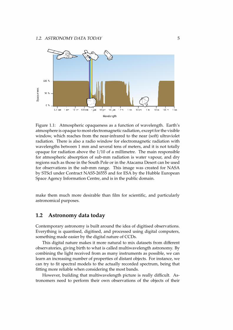
Then came the new windows opened when the space career started, al-lowing humankind, for the first time, to have observatories outside of theatmosphere, which is opaque for radiation other than radio and visible light—see figure 1.1—. We were rewarded with the discovery of strong X-raysources marking active galaxy nuclei, supernovae, and the incredibly brightand distant Gamma-Ray Bursts. By being free of the atmosphere, the Hub-ble Space Telescope has provided us with the deepest view of our Universe,thanks to the repeated, accumulated exposure of the Ultra Deep Field [8].
Of course, our current observatories, both ground-based and space-borne,have only been possible after Charge Couple Devices (CCDs) started to re-place photographic plates. The sensibility of CCDs (measured as their quan-tum efficiency, or percentage of times a photon incidence produces a measur-able change in the sensing element) is much superior to that of photographicplates, allowing the detection of fainter objects. Besides, several other ca-pabilities, specially direct electronic output and linearity in their response,
2In this thesis, we will use light to refer to all kinds of detectable electromagnetic radiation,from the radio band to the gamma rays, and when referring specifically to visible electromag-netic radiation, which our eyes can perceive, we will always use the visible adjective.
1.2. ASTRONOMY DATA TODAY 5
Figure 1.1: Atmospheric opaqueness as a function of wavelength. Earth’satmosphere is opaque to most electromagnetic radiation, except for the visiblewindow, which reaches from the near-infrared to the near (soft) ultravioletradiation. There is also a radio window for electromagnetic radiation withwavelengths between 1 mm and several tens of meters, and it is not totallyopaque for radiation above the 1/10 of a millimetre. The main responsiblefor atmospheric absorption of sub-mm radiation is water vapour, and dryregions such as those in the South Pole or in the Atacama Desert can be usedfor observations in the sub-mm range. This image was created for NASAby STScI under Contract NAS5-26555 and for ESA by the Hubble EuropeanSpace Agency Information Centre, and is in the public domain.
make them much more desirable than film for scientific, and particularlyastronomical purposes.
1.2 Astronomy data today
Contemporary astronomy is built around the idea of digitised observations.Everything is quantised, digitised, and processed using digital computers,something made easier by the digital nature of CCDs.
This digital nature makes it more natural to mix datasets from differentobservatories, giving birth to what is called multiwavelength astronomy. Bycombining the light received from as many instruments as possible, we canlearn an increasing number of properties of distant objects. For instance, wecan try to fit spectral models to the actually recorded spectrum, being thatfitting more reliable when considering the most bands.
However, building that multiwavelength picture is really difficult. As-tronomers need to perform their own observations of the objects of their

6 CHAPTER 1. INTRODUCTION
interest with many different observatories and instruments, something verycostly in terms of both time (observation proposals have to be written, andif approved then the actual observation has to be performed, processed, andanalysed) and effort (spent in learning the different packages needed to reduceastronomical data from different observatories).
Instead, the astronomer can rely on observations previously performedby other astronomers, but that is not easy to accomplish, either: very fewobservatories have archives, and those which have them provide datasetswith very different science requirements. Some observatories provide rawdata, which have to be combined with calibration data for the astronomer toperform the reduction, while others provide already reduced data productswith very little information on how the reduction was performed, whichwere the observing conditions, and so on. Each different archive is accessedthrough its own access portal, has different access policies, different databrowsing mechanisms, and data are finally delivered in different formats.
In the late seventies, the use of digitised imaging, and the need of computer-intensive Fast Fourier Transforms for imaging in radio interferometry madeseveral institutions create, in the late seventies, a common Flexible ImageTransport System, the FITS file format. That data format was presented to thecommunity in 1981 [9], and solved part of the problem of image (and spectral,and tabular data) transport, but the flexibility of the system made FITS filesnot fully compatible between different software packages.
A third source of data for the astronomer are large sky surveys, whichhave started to take place in the last few years, in which data are collected bydedicated wide-field telescopes, with reduction pipelines working for severalspectral bands. The pipelines perform digital processing on the images, anddeterminate tens or hundreds of properties for selected objects. Such is thecase of recent surveys, such as the Sloan Digital Sky Survey (SDSS) [10, 11],such as the Two Micron All Sky Survey (2MASS) [12], but also for the digitisedversion of the Second Palomar Observatory Sky Survey (POSS-II, D-POSS),or even the older, National Geographic Society-Palomar Observatory SkySurvey (NGS-POSSdigitised).
Not all surveys are optical, and there are radio surveys such as the theFIRST [13] and NVSS [14] surveys, performed with the Very Large Arrayradio interferometer (VLA), or the ALFALFA [15, 16], being performed withthe Arecibo radio telescope.
Yet another source of datasets are space-borne satellites. These facilitiesare so expensive, essentially due to the launching costs, that collected datahave to be made available to the community after typically one year of pro-prietary period. The cost of the archive is a small fraction of the operationalcost for the mission, and all space satellites provide some sort of access totheir archives.
1.3. ASTRONOMICAL ARCHIVES: BENEFITS AND PROBLEMS 7
1.3 Astronomical archives: benefits and problems
As pointed in the section before, self-performed observations are but one ofthe ways for astronomers to collect data relevant to their research, while dataarchives, be them originated from the systematic storage of observationaldata from each telescope and instrument, from broad sky surveys, or fromspace-borne missions, conform nowadays the main resource of astronomicaldata.
Archives provide several benefits for astronomers:
Efficiency in resource usage If the observation an astronomer wishes to per-form has already been made, there is no need to go through the fullprocess of writing observation proposals or to wait for the allocatedtime. The data can be downloaded by many different users, servingmany different purposes, some perhaps never considered at the time ofthe observation.
Time domain exploration Some astronomical objects have properties vary-ing in time. Comparing observations taken in different moments allowsto study periodic phenomena (variable stars, asteroid rotation, pulsars,et cetera), or transient phenomena (novae and supernovae, Gamma-RayBursts, et cetera)
Statistical inference Most astronomical processes (specially those regardingextra-galactic astronomy) have time scales much larger than our civili-sation life-span, and our only way to explore them is to take into accountas many objects of the same type as possible. This includes definingobject types, something which can be simplified by data mining tech-niques, which in turn require large datasets to explore.
Non-exclusive access Public archives allow astronomers from countries withlimited research resources to access high-quality data, and produce top-level science.
However, in their current incarnation, archives pose several problems:
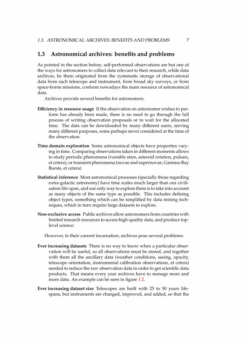
Ever increasing datasets There is no way to know when a particular obser-vation will be useful, so all observations must be stored, and togetherwith them all the ancillary data (weather conditions, seeing, opacity,telescope orientation, instrumental calibration observations, et cetera)needed to reduce the raw observation data in order to get scientific dataproducts. That means every year archives have to manage more andmore data. An example can be seen in figure 1.2.
Ever increasing dataset size Telescopes are built with 25 to 50 years life-spans, but instruments are changed, improved, and added, so that the
8 CHAPTER 1. INTRODUCTIONHow much?The Archive currently holds about 21 TB of active HST and ESO data. In 2002 we distributed about 10 TB in total to users.
How long?The Archive system was initially designed and built in the late 1980s. The first (HST) data became publicly available on January 1st, 1991. Since then VLT and Wide-Field Imager data have become available (late 1990’s) and Archive usage has grown dramatically.
How many users?3000 people are currently registered in the Archive. Each month, about 180 different Archive users and Principal Investigators (PIs) for ESO programmes receive data from us.
How many archive media?The Archive currently comprises about 10,000 different media volumes. The recent, active media currently amount to 4500 DVD-R. The latter are located in 5 different DVD jukeboxes. We also have about 50 200GB magnetic disks in 8 different Linux nodes (the Next Generation Archive System).
Benoît Pirenne, head of the ESO/ST-ECF Science Archive Facility explains:
”The work in the Archive is multi-faceted and comprises, among other things: data input and distribution (manipulation of archive media), the preparation of Principal Investigator packages and overseeing the request queue. The work also includes first line user support and the management of our User Database. Larger projects include copying the entire active data holdings to a new media generation every few years. Technology develops fast, and we have to stay at the forefront! As to the future of the Archive, we should see ever more of the same type of activities. This means that to cope with an ex-pected exponential growth in data volume without increasing the Archive staff significantly, we will have to seek and implement new technical solutions continuously. Efficiency is one of the watchwords for the future. This will have implications for our users as well, as the way data is accessed and distributed may change with time. New techniques are now being developed for the Virtual Observatory that will allow new ways of accessing your data.”
54Evolution of the data distribution volume from the early days until now.
Evolution (past, present and projected future) of the Archive holdings.
OVERVIEW
Figure 1.2: Evolution of the amount of data stored in the ESO archive since1991 to 2003 (in Terabytes in logarithmic scale), together with predictions till2012. Reproduced from [18].
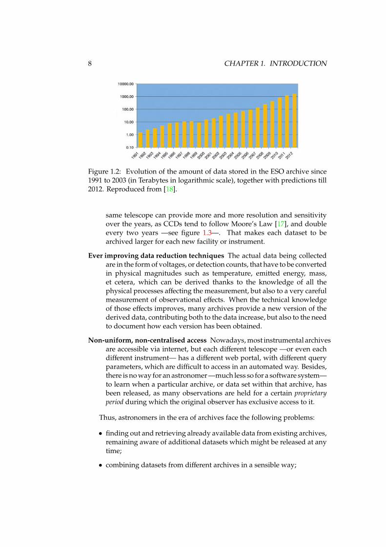
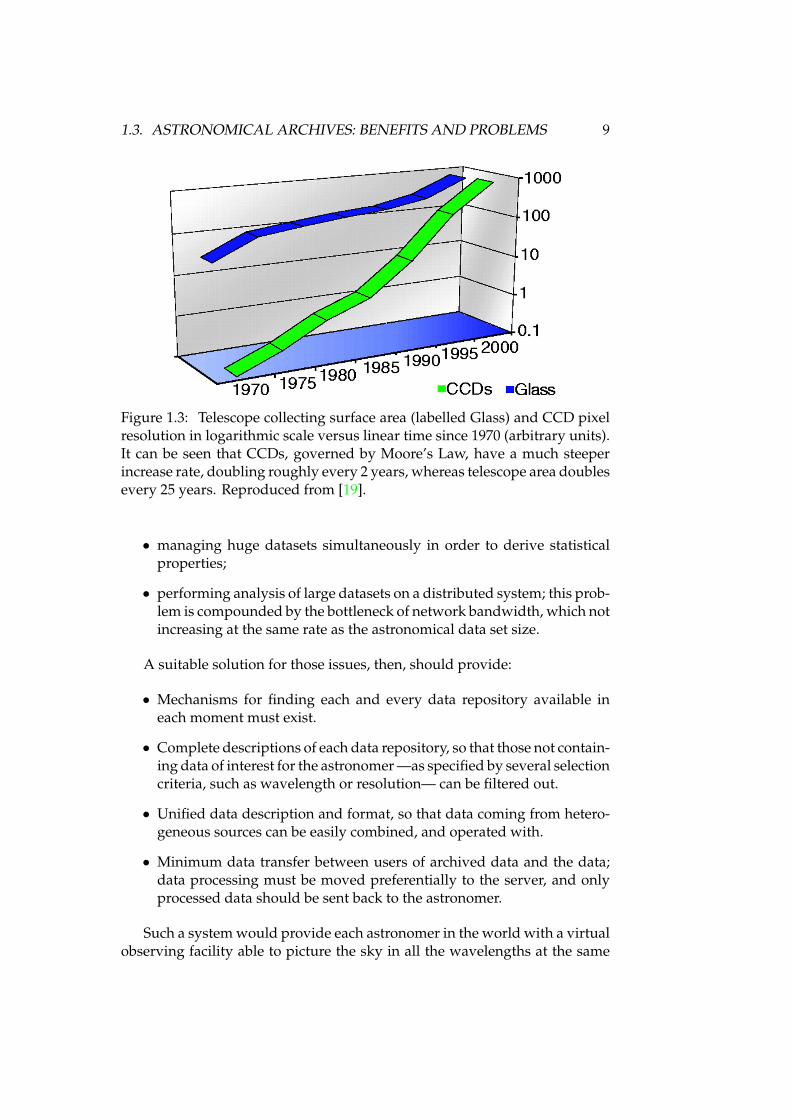
same telescope can provide more and more resolution and sensitivityover the years, as CCDs tend to follow Moore’s Law [17], and doubleevery two years —see figure 1.3—. That makes each dataset to bearchived larger for each new facility or instrument.
Ever improving data reduction techniques The actual data being collectedare in the form of voltages, or detection counts, that have to be convertedin physical magnitudes such as temperature, emitted energy, mass,et cetera, which can be derived thanks to the knowledge of all thephysical processes affecting the measurement, but also to a very carefulmeasurement of observational effects. When the technical knowledgeof those effects improves, many archives provide a new version of thederived data, contributing both to the data increase, but also to the needto document how each version has been obtained.
Non-uniform, non-centralised access Nowadays, most instrumental archivesare accessible via internet, but each different telescope —or even eachdifferent instrument— has a different web portal, with different queryparameters, which are difficult to access in an automated way. Besides,there is no way for an astronomer —much less so for a software system—to learn when a particular archive, or data set within that archive, hasbeen released, as many observations are held for a certain proprietaryperiod during which the original observer has exclusive access to it.
Thus, astronomers in the era of archives face the following problems:
• finding out and retrieving already available data from existing archives,remaining aware of additional datasets which might be released at anytime;
• combining datasets from different archives in a sensible way;
1.3. ASTRONOMICAL ARCHIVES: BENEFITS AND PROBLEMS 9
Figure 1.3: Telescope collecting surface area (labelled Glass) and CCD pixelresolution in logarithmic scale versus linear time since 1970 (arbitrary units).It can be seen that CCDs, governed by Moore’s Law, have a much steeperincrease rate, doubling roughly every 2 years, whereas telescope area doublesevery 25 years. Reproduced from [19].
• managing huge datasets simultaneously in order to derive statisticalproperties;
• performing analysis of large datasets on a distributed system; this prob-lem is compounded by the bottleneck of network bandwidth, which notincreasing at the same rate as the astronomical data set size.
A suitable solution for those issues, then, should provide:
• Mechanisms for finding each and every data repository available ineach moment must exist.
• Complete descriptions of each data repository, so that those not contain-ing data of interest for the astronomer —as specified by several selectioncriteria, such as wavelength or resolution— can be filtered out.
• Unified data description and format, so that data coming from hetero-geneous sources can be easily combined, and operated with.
• Minimum data transfer between users of archived data and the data;data processing must be moved preferentially to the server, and onlyprocessed data should be sent back to the astronomer.
Such a system would provide each astronomer in the world with a virtualobserving facility able to picture the sky in all the wavelengths at the same
10 CHAPTER 1. INTRODUCTION
time, without the need for the astronomer to manually discover each of thedatasets which will conform that picture, or to perform conversions on datacoming from different instruments. That system exists, and is called theVirtual Observatory.
The Virtual Observatory concept was proposed by Jim Gray and AlexSzalay in The World-Wide Telescope [19] in 2001, and the community startedprototyping the system in 2002.
However, many different virtual observatories can be built following thatdefinition. In order to have a single Virtual Observatory where all datasetsand tools are interoperable, standards need to be set and adhered to. Thus astandards sanctioning body is needed, and that is the role of the InternationalVirtual Observatory Alliance (IVOA).
The VO is still in development, but nearing what is called the operationsstage, where astronomers are regularly using VO tools for their research.However, in this thesis will see that there are several problems with thecurrent incarnation of the VO, particularly in the scope of radio astronomy,and multidimensional data access.
1.4 Thesis aim
This thesis is devoted to the study of:
The VO infrastructure Which are the components of the VO, and which arethe interfaces to them, with special emphasis on missing or underdevel-oped blocks for radio astronomical data. This is the scope of chapter 2of Part I.
Modelling radio astronomical data For radio astronomical data to be prop-erly described within the VO data models are needed. Part II is devotedto the RADAMS, the data model developed for radio astronomical ob-servations.
Bringing legacy tools to the VO As there are many man-years of experienceinvested in many already existing astronomical tools, we will study howto incorporate those tools into the VO ecosystem. We have developed aModular VO Interface for Radioastronomy (MOVOIR) which providesboth a GUI for accessing the VO, and tools for adapting legacy tools touse VO protocols. Part III is devoted to it.
Applied work We have used the RADAMS data model as the basis for the as-tronomical archives of the IRAM 30m and DSS-63 70m radio telescopes,and the MOVOIR as the basis for bringing the MASSA and MADCUBAlegacy applications into the VO. We show our results in Part IV is de-voted to the archives which have been built using the RADAMS.
1.5. THESIS CONTEXT 11
As a result of this study, complete VO-compliant radio astronomy modelhas been created, two astronomical archives have been implemented, anda software tool has been developed for allowing legacy radio astronomicaltools access the VO.
1.5 Thesis context
This thesis work has been developed and written within an astrophysicalresearch project (AMIGA3, Analysis of the interstellar Medium of IsolatedGAlaxies) whose objective is studying a sample of isolated galaxies, withmore than 1000 members. A special emphasis is given on radio observationsin the centimetre, millimetre, and sub-millimetre wavelength ranges becausethe (sub)mm spectral band delivers fundamental information to learn aboutphysicochemical processes in the interstellar medium (ISM). It is relevant tonote that astronomy in the (sub)mm range is suffering a strong technologicaladvance, with new astronomical facilities, such as the Sub-Millimetre Array4
(SMA), and the well-advanced construction of the Atacama Large MillimetreArray5 (ALMA).
As public data access in the radio wavelength is limited, we had resolvedto contribute in the building of radio data archives, working together withthe IRAM to provide an archive for the IRAM 30m antenna.
Since our group does intensive analysis of 3D data at all wavelengths(in fact the current trend in spectroscopy), we also decided to collaborate inbringing existing software packages to solve the mentioned tasks, in orderto make our research work more efficient. We have collaborated with JesúsMartín-Pintado’s group at the Molecular and Infrared Astrophysics Depart-ment (DAMIR) of the Institute of Matter Structure, developers of the MASSA(MAdrid Single Spectrum Analysis) and MADCUBA (MADrid CUBe Anal-ysis) tools6 for the Heterodyne Instrument for the Far Infrared7 (HIFI) ofthe soon to be launched Herschel spacecraft8, in order to make both toolscompatible with the VO.
All the problems we need to solve are very similar to those of the astro-nomical community at large (save the emphasis in the radio band), namely:
• easy-to-use data look-up tools, in order to get multi-wavelength datafor every object, to be retrieved from online archives;
• data combination tools, taking into account different data formats, co-ordinate systems, file metadata;
3http://amiga.iaa.csic.es/4http://sma1.sma.hawaii.edu/5http://almaobservatory.org/6Project wiki: http://damir.iem.csic.es/mediawiki-1.12.0/index.php/Portada7http://www.sron.nl/divisions/lea/hifi/8http://herschel.esac.esa.int/

12 CHAPTER 1. INTRODUCTION
• physical parameter extraction tools: each different parameter must in-clude different physics, and needs its own interface.
The community had already started to provide an information-technology-based solution: the Virtual Observatory. All the work performed for thisthesis has been built within that framework.
Chapter 2
The Virtual Observatory
virtualadjective• almost or nearly as described, but not com-
pletely or according to strict definition: thevirtual absence of border controls.
• Computing not physically existing as such butmade by software to appear to do so: a virtualcomputer.
observatorynoun• a room or building housing an astronomical
telescope or other scientific equipment for thestudy of natural phenomena.
• a position or building affording an extensiveview.
The New Oxford American Dictionary, 2nd Edition
2.1 The Virtual Observatory: solving astronomicalarchival issues
In the previous chapter the current status of multi-wavelength, archive basedastronomy was laid as well as the problems arising when dealing with theincreasing number of data archives available to the astronomical community,and with the increasing sizes for each data unit. Additionally, these data unitsmust be combined in order to obtain a multiwavelength view of our universe.
As the archives are already distributed across the world, the solution mustbe network-enabled, and must be as modular as possible, so that different dataproviders and astronomical tool developers can work independently, and
13
14 CHAPTER 2. THE VIRTUAL OBSERVATORY
rely on common interfaces. A Service Oriented Architecture (SOA), wheredata providers create web-services, and tool developers use web-servicesinterfaces to query them fits that description, and allows reuse of alreadyexisting and deployed technology.
It must be noted that astronomical data reduction for large instrumentsis a highly specialised task, and that data reduction techniques are improvedwhen knowledge about the underlying processes (astrophysical and observa-tional) improves. This specialisation, and the long term variability of reduc-tion techniques, makes unfeasible the centralisation of astrophysical archives.
In any case, those services must be oriented to astrophysics, and responsesmust include metadata describing the peculiarities of each data set. Lastly,in order for applications to find out both existing and new services and datasets, a common service registry is needed for VO applications to find outsuitable services and data sets.
Jim Gray and Alexander Szalay, in “The World-Wide Telescope” [19], wereamong the first to outline such a system, which is called the Virtual Obser-vatory (VO). In that paper, they analysed the already mentioned exponentialtrends of instrumental data output and archived data holdings increase, andnoticed the not equally growing gain in astrophysical insight as an unmis-takable sign that astronomers were not being able to cope with the newdata-driven situation, and needed new tools to get the most of the extremelylarge datasets now available to them.
An example of a widely used, very large astronomical dataset is the al-ready mentioned SDSS. In its latest release (DR7), the SDSS consists of morethan 15 TB of image data, plus more than 25 TB of ancillary data, and 18 TB ofcatalogue data. There is not enough bandwidth at the SDSS or at the differentresearch institutions to transfer all the data to all researches which would liketo use the SDSS. And in the future, surveying telescope such as the LargeSynoptic Surveying Telescope (LSST) will produce and process around 7 TBof raw data per night.
Exploiting this ever-increasing amount of data is only feasible by scientific-case guided data selection, together with automated data mining techniques.But for that to be performed in a fully automated way, data archives and dataanalysis tools must become interoperable.
For achieving the interoperability we will need, as stated by F. Genova inher “Interoperability” article [20]:
• common data formats;
• common data access protocols; and
• common data models for the same type of observations, as independentas possible of the generation of the dataset, so that data from verydifferent observatories and instruments can be combined.

2.2. VO ARCHITECTURE AND PHILOSOPHY 15
In addition, as VO services are distributed across the globe, and can bedeployed anywhere, anytime, one or several services registries are needed,so that
But for those common formats, protocols and data model to become trulycompatible an standardisation body is needed. In the VO, that body is theInternational Virtual Observatory Alliance.
In the next sections we will see how the VO achieves archive interoper-ability, which mechanisms provides for minimising local data processing asmuch as possible, and what is the high level organisation of the IVOA.
2.2 VO architecture and philosophy
In Gray and Szalay’s paper [19], the stated philosophy for the VO is that ofan e-infrastructure1 which makes all astronomical data in the world availablefor astronomers as if they were in their own desktop, without the limitationsof desktop computing.
For many large datasets the user should not deal with the data directly, asthe data transport time for many modern datasets is not negligible, and thedata producer’s infrastructure can be better suited for remote processing. Intime, remote processing has to become commonplace, as it will become theonly solution to let users ask questions to datasets much larger than typicalworkstation can manipulate, avoiding network bottlenecks at the same time.
In any case, sufficient metadata must be provided so that astronomers donot need to download data to see if they can be useful or interesting, andperform instead a suitable selection of datasets based on metadata. In par-ticular, data quality assessment through metadata inspection and evaluationallows astronomers not to retrieve, for instance, low resolution datasets if theyneed precise astrometric measurements, while other astronomers interestedon obtaining upper limits of an object’s emissions might find them useful.
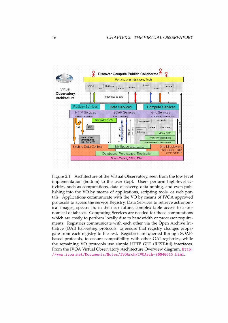
How is that vision actually implemented? Figure 2.1 portraits a simplified,all-encompassing vision of the Virtual Observatory. In that figure we seethe Virtual Observatory from the lowest level supporting implementation(network cabling, routers, storage media, et cetera; what is usually knownas the iron), to base internet protocols, and grid computing middleware, toVO services and protocols implemented on top of that infrastructure, andapplications using both services and protocols to present the user with aunified interface.
It is legitimate to ask how far is the Virtual Observatory today from beingcompletely transparent to the user. The answer to that is that there are several
1The e in e-infrastructure does not stand for electronic, but for enhanced, as in e-Science, orenhanced science. The enhancement is produced by means of the massive use of networkedresources, such as data grids, computation grids, distributed storage, et cetera, which conformthe e-infrastructure.
16 CHAPTER 2. THE VIRTUAL OBSERVATORY
Figure 2.1: Architecture of the Virtual Observatory, seen from the low levelimplementation (bottom) to the user (top). Users perform high-level ac-tivities, such as computations, data discovery, data mining, and even pub-lishing into the VO by means of applications, scripting tools, or web por-tals. Applications communicate with the VO by means of IVOA approvedprotocols to access the service Registry, Data Services to retrieve astronom-ical images, spectra or, in the near future, complex table access to astro-nomical databases. Computing Services are needed for those computationswhich are costly to perform locally due to bandwidth or processor require-ments. Registries communicate with each other via the Open Archive Ini-tiative (OAI) harvesting protocols, to ensure that registry changes propa-gate from each registry to the rest. Registries are queried through SOAP-based protocols, to ensure compatibility with other OAI registries, whilethe remaining VO protocols use simple HTTP GET (REST-ful) interfaces.From the IVOA Virtual Observatory Architecture Overview diagram, http://www.ivoa.net/Documents/Notes/IVOArch/IVOArch-20040615.html.
2.3. VO DATA FORMATS 17
factors which make the Virtual Observatory still a separate environment forastronomical research:
• VO applications and portal are still unknown to many astronomicalusers, including some data providers. The different VO groups aremaking an effort in the dissemination of the VO concept, both for as-tronomical users and data providers. Many different workshops andschools are being promoted in order to reach users and providers.
• Many interesting datasets are still not available via the VO. The NVOand the Euro-VO projects, are developing tools to make data publish-ing easier for small research groups. However, they demand a highlevel of computing expertise in the domain of networking, web servicestechnologies, XML, and of the inner workings of the VO. Besides, a com-mitment to maintain the archive operational in the long term means theresearch group has to keep storage and network resources with a highlevel of availability. This makes it difficult for those small groups tobecome data publishers if they do not deploy a complete archive.
• Many different useful tools for astronomers predate the Internet era,with many legacy tools unable to access Virtual Observatory datasets.
2.3 VO data formats
One of the three key aspects of interoperability, as we have seen,is dataformats. If applications do not know how to operate with the files containingthe data relevant to them it does not matter if data was compliant with a givendata model, or if it was accessible from a common access protocol.
The FITS data format
It was radio astronomy, in particular radio interferometry, which started withthe need for a common data format. Interferometric observations provideastronomical images by means of the inverse Fourier Transform of a sparselysampled 2D Fourier expansion. As reconstruction algorithms needed ex-pensive equipment and long processing times to provide the images, andlater additional cleaning algorithms had to be run, it made sense to create acommon data format which allowed for the interchange of scientific gradeastronomical image (and visibilities) products, so that data could be movedto powerful enough computers. That format is the Flexible Image TransportSystem (FITS), created in the late seventies, and finally published in 1981 [9].
The main benefit from the FITS file format was the decoupling of ac-tual instrument data from data about the instrument and observation setup(metadata). Data resided in image or table extensions, while metadata was

18 CHAPTER 2. THE VIRTUAL OBSERVATORY
expressed in the form of ASCII headers, such as TELESCOP for specifying anobservatory, or INSTRUME for specifying a particular instrument within thatobservatory.
However, the FITS file format, over the years, developed its own share ofproblems:
• Only a small core vocabulary is defined. Additional headers can beused in non-standard ways. The IAU Working Group in charge of thefile format does not mandate particular keywords, or proposes bestpractices for FITS archival.
• Multiplicity of de facto per instrument and per package FITS standards:for instance, the AIPS++ radio interferometry reduction program uses aconvention called FITS-IDI [21] (FITS Interferometry Data Interchange),while AIPS, its ancestor, uses the UVFITS convention. On the sin-gle dish side, IRAM uses the IMB-FITS format [22], while others usethe SDFITS [23] (Single Dish FITS) convention. That means that ob-servation metadata, such as calibration curves, tipping measurements(skydips), et cetera, could be included with the file as additional tablesor not, depending on observatory, and some times depending on theinstrument.
• FITS is not an appropriate file format for archival purposes. Thereis a flat header for all extensions, and it is physically joined to thecorresponding metadata. In order to index a FITS archive, additionallayers have to be applied.
• FITS files cannot be streamed on the fly from an instrument: given thefact that FITS is block oriented (due to its origin as an image transportformat using computer tapes), it is very difficult to generate a valid FITSfile from a continuous stream of data. At most, different FITS files can becreated for different runs of an observation (per scan, or per integration),and then written down as a FITS file. But a truncated FITS file isvery difficult to recover without manual tweaking, or to be interpretedautomatically, apart from the ASCII Header part. Conversely, FITS filescannot be read sequentially, either, and a FITS file needs to be completelyread (apart from the Header), in order to interpret its data.
• There is no way to combine data from different instruments, as unitsand scales are specified in a human readable, but not computer under-standable form.
The latest Definition of the Flexible Image Transport System (FITS) docu-ment [24] still includes phrases referring to some features of the FITS fileformat as legacy, but used by the earlier packages, while new instruments
2.3. VO DATA FORMATS 19
use additional mechanisms not compatible with those used by the oldesttools. It is not uncommon (or unheard of) needing to manually change FITSfiles, or file generation parameters, to make FITS files read from an archive,or observed from other instruments, compatible with particular tools.
With all of its shortcomings, the fact that FITS files allow for the storage ofimages, spectra, and other tables, with additional metadata describing thosedata products, has been enormously beneficial for the astronomical commu-nity, as it has made data distribution and tools development considerablyeasier.
Besides, the main capabilities of the FITS file format, which make it themost successful data format in astronomy to date, and is still in wide usetoday (to the point of being an integral part of the VO), are the following:
Flexibility At the same time FITS weakness and strength, the format flexi-bility2 has allowed it to respond to the changing needs in astronomy,transporting data both from ground-based and space-born optical tele-scopes’ images, radio telescope single dish spectra, maps or On-The-Flyobservations, radio interferometer visibility, imaging, and data cubes,optical Fabry-Perot interferometer data cubes, Integral Field Units 3Dspectroscopy, et cetera. The array of different telescopes and instru-ments using the FITS file format comprises the entire observationalcommunity.
Large availability of support libraries From the beginning, astronomy soft-ware developers could rely on fitsio3, a FITS read and write librarywith access to the full array of capabilities of the FITS data format.That library was written in FORTRAN, but soon a cfitsio library wasreleased for C/C++ development. For Java, support is provided bythe nom.tam.fits4 library, and for Python a NumPy-compatible PyFITS5
library exists.
There are a large number of archives providing FITS files, and for the VOto be successful, and have those archives provide VO compatibility, the VOmust accommodate FITS files.
2FITS flexibility is based on the ability of FITS files of containing an arbitrary numberof multidimensional arrays, each one with its own FITS headers for describing its content.However, it is not possible to specify whether different arrays are related in any way. Forinstance, if one of the arrays corresponds to a reduced spectrum, and another one correspondsto sky spectrum which has been subtracted, the only way to know it would be by manualinspection of the FITS file.
3http://heasarc.gsfc.nasa.gov/docs/software/fitsio/fitsio.html4http://heasarc.gsfc.nasa.gov/docs/heasarc/fits/java/v0.9/5http://www.stsci.edu/resources/software_hardware/pyfits
20 CHAPTER 2. THE VIRTUAL OBSERVATORY
The VOTable
Any new data format wishing to achieve the same diffusion as FITS needsto keep FITS’ main strengths —flexibility, and availability of libraries andtools—, while addressing most of its shortcomings.
The VOTable is the main VO data format for the interchange both oftabular data, and of metadata related to any kind of astronomical data, andhas the following properties:
XML data format The VOTable is an XML-based data format, and as such,it earns a wide availability of data writing and consumption libraries.XML documents can be queried through the XQuery language, or trans-formed in different kind of documents with XML Style-sheet Transfor-mations (XSLTs). Plus, XML documents and processors are inherentlyinternet-ready, providing mechanisms for linking with datasets locatedanywhere in the internet. Prior to the VOTable, different attempts atcombining XML with FITS files had been made [25, 26], and other XML-based based file formats [27, 28] had been devised to replace FITS files.
Namespace support Stemming from its XML origin, VOTables can embedterms from different namespaces, thus allowing further flexibility andextensibility, without losing the origin and semantics of the extension.
Data and metadata separation VOTables are much more verbose than FITSfiles —something common to all XML-based data formats—, and typicaldata sizes are bigger. However, the linking mechanism allows XML-metadata to be processed and queried without having to download theactual astronomical data. What is more, particular FITS sections can bereferenced from any VOTable, so that different VOTables can point tothe same table of a FITS file, or the same VOTable can point to differenttables of the same FITS file.
Astronomical and astrophysical semantics VOTables have astronomy spe-cific tags, such as coordinate system definitions, but FIELD elementscan optionally provide units attributes, and for the clarification of thegeneral kind of information in each field, a ucd attribute —short forUniversal Content Descriptor, UCD— can be used. We will see thatthe UCDs provide metadata with semantics which come from IVOAdefined data models, and that additional utype attributes can be usedto further specify a particular field within a particular data model.
Support for FITS file linking The VOTable can hold data by itself, but thelinking mechanisms are typically used for providing internet access toFITS files.
2.4. VO DATA ACCESS PROTOCOLS 21
Figure 2.2 shows an example VOTable obtained from the AMIGA VOcatalog, with the metadata for the description of a four column table, withthree rows returned.
The complete definition of the VOTable, in terms of its XML DocumentType Definition (DTD), and an XML Schema, can be found in appendix C.
2.4 VO data access protocols
The common file format helps in the data interchange between different sys-tems, and in letting different applications share data. However, in order toretrieve those data from the different archives existing in the VO, commondata access protocols are needed.
Then main astronomical data products produced as astronomical obser-vation facilities are the reduced image, and the reduced 1D spectra. Workingwith those images and spectra, different properties of objects in the universe,such as temperature, distance, diameter, or more directly, received flux, PointSpread Function (PSF), et cetera, can be derived, and positional cataloguescreated.
For those kinds of data the initial VO protocols to be created were theSimple Image Access Protocol [29] (SIAP) and the Simple Spectral AccessProtocol [30, 31] (SSAP). For catalogues the Simple Cone Search (SCS, orConeSearch) protocol [32] was devised, with the idea of retrieving table rowsfrom positional catalogues centred around a certain position, and from acertain angular distance from the centre (hence the Cone in the protocolname).
Apart from data-product driven access protocols, an additional data ac-cess protocol is needed for querying the VO Registry. That protocol is basedon the Open Archives Initiative
You can find a brief description of each protocol interface in appendix Dfor quick reference.
2.5 VO data models
With a common data format and a common data access protocol astronomerswould be able to access different archives using automated tools, and the datacould be sent to different applications.
However, astrophysical datasets are very complex in nature, and with theflexibility of the VOTable or the FITS file formats many different files canbe constructed which contain the same astrophysical information, but in aincompatible form.
A data model is a description of the set of entities needed for informationstorage in a particular field, and specifies both the data being stored, and therelationships between them.
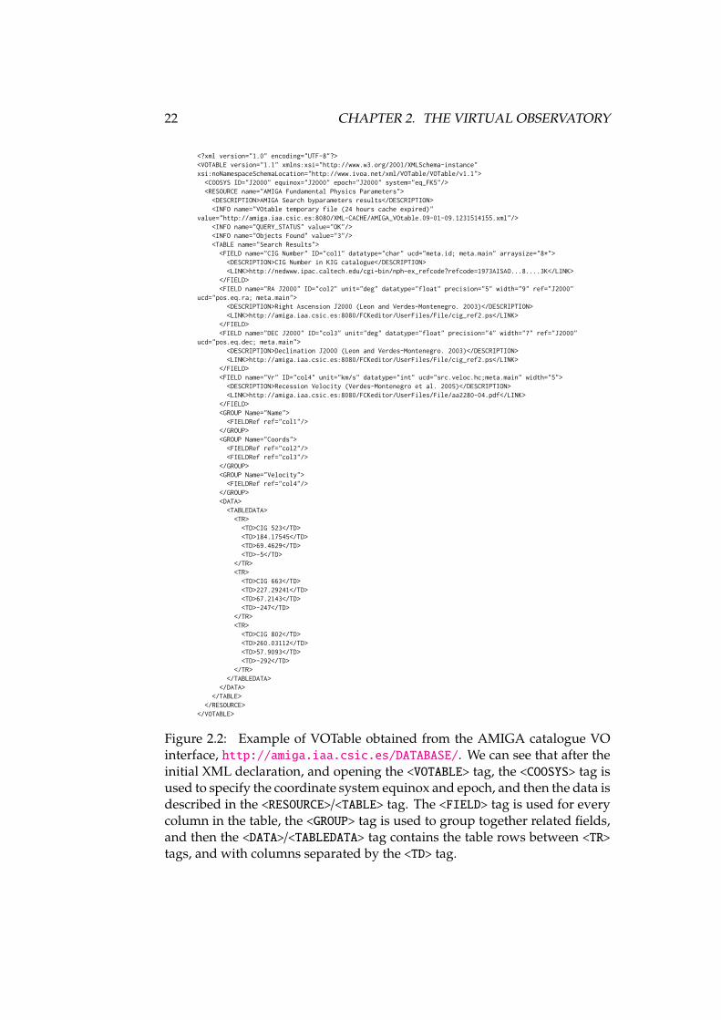
22 CHAPTER 2. THE VIRTUAL OBSERVATORY
- 1/1 -
<?xml version="1.0" encoding="UTF-8"?><VOTABLE version="1.1" xmlns:xsi="http://www.w3.org/2001/XMLSchema-instance"xsi:noNamespaceSchemaLocation="http://www.ivoa.net/xml/VOTable/VOTable/v1.1"> <COOSYS ID="J2000" equinox="J2000" epoch="J2000" system="eq_FK5"/> <RESOURCE name="AMIGA Fundamental Physics Parameters"> <DESCRIPTION>AMIGA Search byparameters results</DESCRIPTION> <INFO name="VOtable temporary file (24 hours cache expired)"value="http://amiga.iaa.csic.es:8080/XML-CACHE/AMIGA_VOtable.09-01-09.1231514155.xml"/> <INFO name="QUERY_STATUS" value="OK"/> <INFO name="Objects Found" value="3"/> <TABLE name="Search Results"> <FIELD name="CIG Number" ID="col1" datatype="char" ucd="meta.id; meta.main" arraysize="8*"> <DESCRIPTION>CIG Number in KIG catalogue</DESCRIPTION> <LINK>http://nedwww.ipac.caltech.edu/cgi-bin/nph-ex_refcode?refcode=1973AISAO...8....3K</LINK> </FIELD> <FIELD name="RA J2000" ID="col2" unit="deg" datatype="float" precision="5" width="9" ref="J2000"ucd="pos.eq.ra; meta.main"> <DESCRIPTION>Right Ascension J2000 (Leon and Verdes-Montenegro. 2003)</DESCRIPTION> <LINK>http://amiga.iaa.csic.es:8080/FCKeditor/UserFiles/File/cig_ref2.ps</LINK> </FIELD> <FIELD name="DEC J2000" ID="col3" unit="deg" datatype="float" precision="4" width="7" ref="J2000"ucd="pos.eq.dec; meta.main"> <DESCRIPTION>Declination J2000 (Leon and Verdes-Montenegro. 2003)</DESCRIPTION> <LINK>http://amiga.iaa.csic.es:8080/FCKeditor/UserFiles/File/cig_ref2.ps</LINK> </FIELD> <FIELD name="Vr" ID="col4" unit="km/s" datatype="int" ucd="src.veloc.hc;meta.main" width="5"> <DESCRIPTION>Recession Velocity (Verdes-Montenegro et al. 2005)</DESCRIPTION> <LINK>http://amiga.iaa.csic.es:8080/FCKeditor/UserFiles/File/aa2280-04.pdf</LINK> </FIELD> <GROUP Name="Name"> <FIELDRef ref="col1"/> </GROUP> <GROUP Name="Coords"> <FIELDRef ref="col2"/> <FIELDRef ref="col3"/> </GROUP> <GROUP Name="Velocity"> <FIELDRef ref="col4"/> </GROUP> <DATA> <TABLEDATA> <TR> <TD>CIG 523</TD> <TD>184.17545</TD> <TD>69.4629</TD> <TD>-5</TD> </TR> <TR> <TD>CIG 663</TD> <TD>227.29241</TD> <TD>67.2143</TD> <TD>-247</TD> </TR> <TR> <TD>CIG 802</TD> <TD>260.03112</TD> <TD>57.9093</TD> <TD>-292</TD> </TR> </TABLEDATA> </DATA> </TABLE> </RESOURCE></VOTABLE>
Figure 2.2: Example of VOTable obtained from the AMIGA catalogue VOinterface, http://amiga.iaa.csic.es/DATABASE/. We can see that after theinitial XML declaration, and opening the <VOTABLE> tag, the <COOSYS> tag isused to specify the coordinate system equinox and epoch, and then the data isdescribed in the <RESOURCE>/<TABLE> tag. The <FIELD> tag is used for everycolumn in the table, the <GROUP> tag is used to group together related fields,and then the <DATA>/<TABLEDATA> tag contains the table rows between <TR>tags, and with columns separated by the <TD> tag.
2.6. VO APPLICATIONS 23
For the VO, there are several kinds of data models which can be built:
A general data model for astronomical observations such a data model wouldbe centred around the idea of astronomical observation and data reduc-tion setup.
Data model for individual data products these data data models would ex-ist for the different data products created with the different astronomicalinstruments: images, spectra, data cubes (collections of images or spec-tra), photometric data, et cetera.
In order to identify that a particular datum, appearing anywhere in a VOdataset, has a precise astronomical meaning the Unified Content Descrip-tors (UCDs) where created. They conform a controlled vocabulary whoseprecise meaning is set by the IVOA, and allow, for instance, to identify if atable column corresponds to flux in a particular radio band, or provides anastronomical coordinate, and so on.
We will see in Part II that the data modelling effort is still ongoing withinthe VO, and one of the main contributions of this thesis is a complete obser-vation data model for radio astronomy, with some parts usable for non radioastronomical observations. More detail in UCDs will be offered there.
2.6 VO applications
VO data formats, access protocols, and data models are the infrastructure onwhich the rest of the VO can rely. We call VO application to any softwarepackage of any kind which makes uses of existing VO services to perform thevisualisation of data in VO format, queries of VO services, or even computa-tions on existing datasets either in VO format, or retrieved from the VO.
Table 2.1 provides a non exhaustive list of applications which providesome form of VO compatibility.
2.7 VO application messaging
The data access protocols mentioned in section 2.4 need the deployment ofa full-featured web server. However, in a local machine, with several VOapplications running at the same time, and with all of them understandingVOTables and FITS files, a simple messaging protocol between applicationswould allow them to notify, or be notified, that some data is available, and ifthe messaging protocol supported it, several applications in communicationcould be showing different but interacting views of the same data.
Such a messaging protocol was prototyped and was initially known asthe PLatform for Astronomical Tool InterConnection (PLASTIC), and imple-mented in many different VO applications, such as TOPCAT, or the Aladin
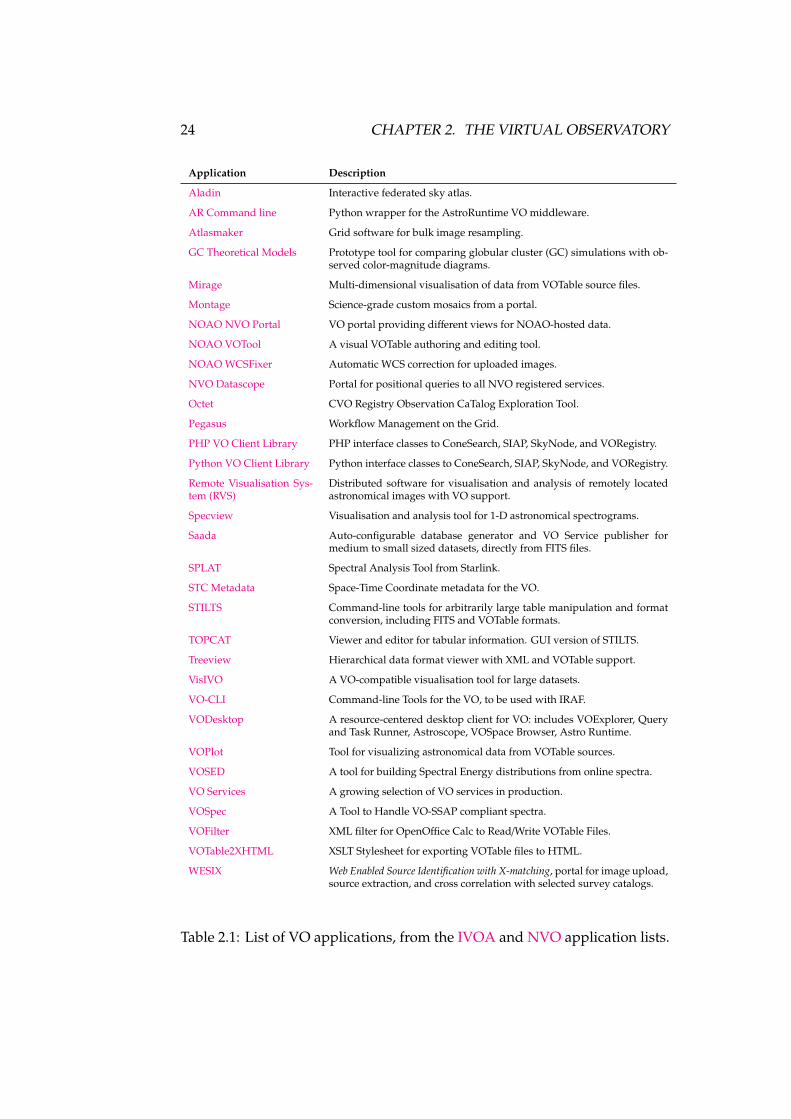
24 CHAPTER 2. THE VIRTUAL OBSERVATORY
Application Description
Aladin Interactive federated sky atlas.
AR Command line Python wrapper for the AstroRuntime VO middleware.
Atlasmaker Grid software for bulk image resampling.
GC Theoretical Models Prototype tool for comparing globular cluster (GC) simulations with ob-served color-magnitude diagrams.
Mirage Multi-dimensional visualisation of data from VOTable source files.
Montage Science-grade custom mosaics from a portal.
NOAO NVO Portal VO portal providing different views for NOAO-hosted data.
NOAO VOTool A visual VOTable authoring and editing tool.
NOAO WCSFixer Automatic WCS correction for uploaded images.
NVO Datascope Portal for positional queries to all NVO registered services.
Octet CVO Registry Observation CaTalog Exploration Tool.
Pegasus Workflow Management on the Grid.
PHP VO Client Library PHP interface classes to ConeSearch, SIAP, SkyNode, and VORegistry.
Python VO Client Library Python interface classes to ConeSearch, SIAP, SkyNode, and VORegistry.
Remote Visualisation Sys-tem (RVS)
Distributed software for visualisation and analysis of remotely locatedastronomical images with VO support.
Specview Visualisation and analysis tool for 1-D astronomical spectrograms.
Saada Auto-configurable database generator and VO Service publisher formedium to small sized datasets, directly from FITS files.
SPLAT Spectral Analysis Tool from Starlink.
STC Metadata Space-Time Coordinate metadata for the VO.
STILTS Command-line tools for arbitrarily large table manipulation and formatconversion, including FITS and VOTable formats.
TOPCAT Viewer and editor for tabular information. GUI version of STILTS.
Treeview Hierarchical data format viewer with XML and VOTable support.
VisIVO A VO-compatible visualisation tool for large datasets.
VO-CLI Command-line Tools for the VO, to be used with IRAF.
VODesktop A resource-centered desktop client for VO: includes VOExplorer, Queryand Task Runner, Astroscope, VOSpace Browser, Astro Runtime.
VOPlot Tool for visualizing astronomical data from VOTable sources.
VOSED A tool for building Spectral Energy distributions from online spectra.
VO Services A growing selection of VO services in production.
VOSpec A Tool to Handle VO-SSAP compliant spectra.
VOFilter XML filter for OpenOffice Calc to Read/Write VOTable Files.
VOTable2XHTML XSLT Stylesheet for exporting VOTable files to HTML.
WESIX Web Enabled Source Identification with X-matching, portal for image upload,source extraction, and cross correlation with selected survey catalogs.
Table 2.1: List of VO applications, from the IVOA and NVO application lists.
2.8. VO RESOURCE REGISTRY 25
Sky Atlas. The shortcomings of the PLASTIC protocol gave birth to the SimpleApplication Messaging Protocol (SAMP), now in Proposed Recommendationstage.
The SAMP messaging protocol is described in section 10.3.
2.8 VO resource registry
The only way VO clients can remain aware of existing and newly incorporatedservices is by means of a registration point were public data services areannounced.
In the VO, there is no centralised, preferential registry. Instead, manyregistries exist, but with the ability to harvest entries from other registries, sothat there can exist specialised registries on one hand, and shared registriesentries on the other.
VO registry and harvesting infrastructure has been built around the OpenArchives Initiative6 (OAI) standard resource registries, so that an already inplace infrastructure could be leveraged. The OAI has developed a Protocol forMetadata Harvesting (OAI-PMH) [33], that allows OAI registries to harvestother OAI registries they might know about (with an entry in their ownregistry, for instance), so that VO resources can be entered in one registry, andthey should propagate to any other OAI-PMH compliant registries.
That allows VO tools to point to a single harvesting registry, and restassured that VO servers will be found in any of those registries.
Registered resources (OAI-PHM records) provide at least the Dublin Coremetadata set [34], which specifies resource types, publishers, curators, etcetera. Additionally, service-specific resource profiles exist for the differentdata access service types, and include astronomical data for service such asthe sky region covered by the observation —footprint—, wavelength, instru-ments providing the data, et cetera.
In particular, the VOResource [35] XML Schema has been developed asthe acceptable OAI-PHM record formats for generic VO registries, and theVODataService schema [36] is in development to further standardise dataservice entries.
Several VO registries provide web pages to query the registries apart fromthe usual OAI-PHM interface, such as the NVO Carnivore7, or the ESA-VOregistry8.
6http://www.openarchives.org/7http://nvo.caltech.edu:8080/carnivore/8http://esavo.esa.int/registry/
26 CHAPTER 2. THE VIRTUAL OBSERVATORY
2.9 Standardising the VO: the International VirtualObservatory Alliance (IVOA)
As previously stated, for VO common data formats, interfaces, and datamodels to become truly standard requires a standards enforcing authority,and within the VO the International Virtual Observatory Alliance (IVOA)is the organisation in charge of developing and sanctioning interoperabilitystandards.
The International Virtual Observatory Alliance was created in 2002, afterthe first national VO associations realised that they needed to keep work-ing together, and than an international standards-setting organisation wasneeded to sanction Virtual Observatory standards, steer the development ofnew ones, and foster the spread of the VO to most data providers.
The IVOA founders were the US National Virtual Observatory (NVO), theEuropean (AVO) and supporting centres —Centre de Données astronomiquesde Strasbourg (CDS), AstroGrid, German Astrophysical Virtual Observatory(GAVO)—, the Russian Virtual Observatory (RVO), VO-India, e-AstronomyAustralia (eAA; later Australian Virtual Observatory, Aus-VO) and the Cana-dian Virtual Observatory (CVO), which in 2002 met at the ESO Headquartersin Garching, and agreed in forming the International Virtual ObservatoryAlliance, following the statement drafted by Peter Quinn, Robert Hanisch,and Andy Lawrence [37]. The minutes of that meeting can be found in [38],and the conference proceedings compiled in the book Toward an InternationalVirtual Observatory [39].
Following that initial meeting, several services were created, and Aladinwas provided with a VO interface, giving birth to the first AstrophysicalVirtual Observatory (AVO) prototype [40].
The inspiration for the IVOA organisation is the World Wide Web Con-sortium9 (W3C), in the sense of providing the steering effort for standards tobe agreed upon within different Working Groups (WGs), so that there is anofficial forum in which such standards are proposed, discussed, and finallyapproved. The main difference with the W3C is that the latter is pay per play—W3C participants pay in order to influence the standardisation process—,while the IVOA is open to any interested party with expertise in a given field.
Presently , the IVOA is formed by 16 VO projects from all over the world10,from Armenia, Australia, Canada, China, Europe, France, Germany, Hun-gary, India, Italy, Japan, Korea, Russia, Spain, the United Kingdom, and theUnited States (see figure 2.3). Membership is open to additional national andinternational projects11.
9http://w3c.org/10http://ivoa.net/pub/members/11 VO projects wishing to join the IVOA must follow the IVOA Guidelines for Participation
http://ivoa.net/Documents/latest/IVOAParticipation.html.
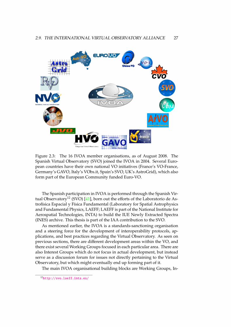
2.9. THE INTERNATIONAL VIRTUAL OBSERVATORY ALLIANCE 27
Figure 2.3: The 16 IVOA member organisations, as of August 2008. TheSpanish Virtual Observatory (SVO) joined the IVOA in 2004. Several Euro-pean countries have their own national VO initiatives (France’s VO-France,Germany’s GAVO, Italy’s VObs.it, Spain’s SVO, UK’s AstroGrid), which alsoform part of the European Community funded Euro-VO.
The Spanish participation in IVOA is performed through the Spanish Vir-tual Observatory12 (SVO) [41], born out the efforts of the Laboratorio de As-trofísica Espacial y Física Fundamental (Laboratory for Spatial Astrophysicsand Fundamental Physics, LAEFF; LAEFF is part of the National Institute forAerospatial Technologies, INTA) to build the IUE Newly Extracted Spectra(INES) archive. This thesis is part of the IAA contribution to the SVO.
As mentioned earlier, the IVOA is a standards-sanctioning organisationand a steering force for the development of interoperability protocols, ap-plications, and best practices regarding the Virtual Observatory. As seen onprevious sections, there are different development areas within the VO, andthere exist several Working Groups focused in each particular area. There arealso Interest Groups which do not focus in actual development, but insteadserve as a discussion forum for issues not directly pertaining to the VirtualObservatory, but which might eventually end up forming part of it.
The main IVOA organisational building blocks are Working Groups, In-
12http://svo.laeff.inta.es/
28 CHAPTER 2. THE VIRTUAL OBSERVATORY
IVOA
Working Groups
Applications
Data Access Layer
Data Modelling
Grid & Web Services
Resource Registry
Semantics
VO Events
VO Query Language
VOTable
Interest Groups
Radio (obsolete)Data Curation &
Preservation
Theory
OGF AstroRG
Steering & Coordination
IVOA Executive
Technical Coordination Group
Standing Committee on Standards & Processes
Figure 2.4: IVOA organisational building blocks: Working Groups, InterestGroups, and Coordination boards. The IVOA activity for standards devel-opment is performed in the Working Groups, while Interest Groups gathertogether IVOA users with common interests outside the Virtual Observatory(such as the Open Grid Forum, or the Data Curation and Preservation interestgroups), or outside existing Working Groups (such as the Radio astronomy oror Theory interest groups). The Steering & Coordination bodies provide themain direction for IVOA activities, technical coordination across the existingWorking Groups (i.e., Data Modelling and Data Access Layer in the devel-opment of interoperable protocols and data set access tools), and take care ofpossible changes to existing standards.
terest Groups, and Coordination and steering committees. Their detaileddiscussion can be found in Appendix A. Figure 2.4 shows graphically thehigh-level organisation of the IVOA.
IVOA Working Groups are not completely equal in scope. Most of themhave to do with particular parts of the IVOA, as seen in figures 2.1 and 2.9.
2.10. THE VO FROM THE POINT OF VIEW OF DIFFERENT ACTORS 29
2.10 The VO from the point of view of different actors
Which parts of the Virtual Observatory do users interact with? What does aparticular astronomer need to know?
In the following subsections we will offer several portraits of the VO asseen from the points of view of different actors: the astronomical user, theapplication developer, the data provider, and the data service developer.
The VO from the user’s point of view
For a non-technical user (one who wishes to use the VO via standard tools,and does not wish to access directly the VO infrastructure), the VO can beseen just as a set of portals (applications or web sites) which access all ofthe services and data available in the Virtual Observatory. Some of themmight also retrieve additional data from non-VO-compliant archives, andeven mix them with local datasets. Users would launch different VO applica-tions depending of the tasks they might wish to perform (Aladin Sky Atlas13
for catalogue and image queries; TOPCAT14 for catalogue and table ma-nipulation; VOSpec15, SpecView16 or SPLAT-VO17 for spectra manipulation;VODesktop18 for Registry queries, remote task execution, and access to theVOSpace; or web portals such as the NVO Datascope19 for all-encompassingbrowser-based archive searches). See figure 2.5 for a conceptual diagram ofthe VO for astronomers.
This can be better explained by means of an example. Imagine Alice isan astronomer who has already been introduced to the VO, and that she issearching for catalogues, images, and spectra on σ-orionis, a star-formingregion in the Orion belt.
She would fire up a tool such as the Aladin Sky Atlas, and use the searchbox to either specify the coordinates of the zone she is interested in, or wouldjust write sigma orionis, and let Aladin query a name solver service, suchas Sesame, to come up with the coordinates.
After having set the coordinates, Alice could set an angular radius for thesearch of interesting datasets, setting the separation for objects in the vicinity,or could just use the default radius. Aladin would ask different archives forboth images and catalogues, laying catalogue data with coordinate informa-tion on top of the retrieved images, which can be composed from severalbands.
13http://aladin.u-strasbg.fr/14http://www.star.bris.ac.uk/~mbt/topcat/15http://esavo.esa.int/vospec/16http://www.stsci.edu/resources/software_hardware/specview17http://www.astrogrid.org/wiki/Install/Downloads18http://www.astrogrid.org/wiki/Install/Downloads19http://heasarc.gsfc.nasa.gov/vo/
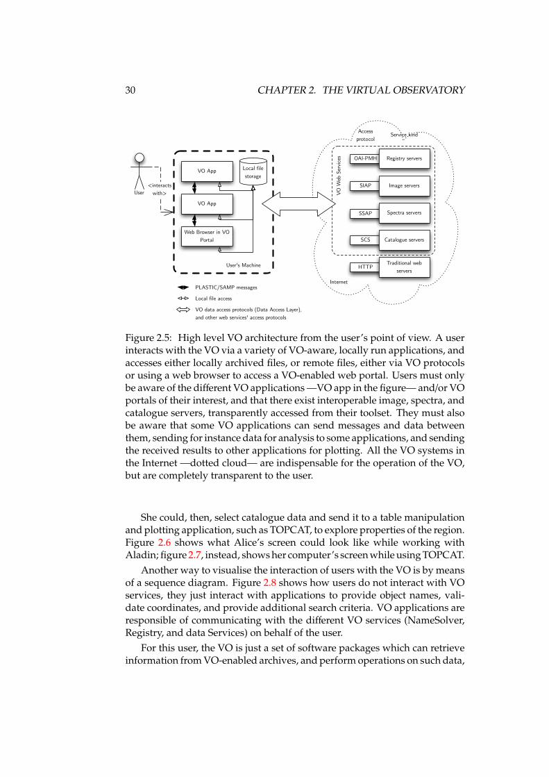
30 CHAPTER 2. THE VIRTUAL OBSERVATORY
<interacts with>User
VO App
VO App
Web Browser in VO Portal
User's Machine
PLASTIC/SAMP messages
OAI-PMH Registry servers
SIAP
SSAP
SCS
HTTP
Image servers
Spectra servers
Catalogue servers
Traditional web servers
VO W
eb S
ervi
ces
Internet
Local file storage
Local file access
VO data access protocols (Data Access Layer),and other web services' access protocols
Service kindAccessprotocol
Figure 2.5: High level VO architecture from the user’s point of view. A userinteracts with the VO via a variety of VO-aware, locally run applications, andaccesses either locally archived files, or remote files, either via VO protocolsor using a web browser to access a VO-enabled web portal. Users must onlybe aware of the different VO applications —VO app in the figure— and/or VOportals of their interest, and that there exist interoperable image, spectra, andcatalogue servers, transparently accessed from their toolset. They must alsobe aware that some VO applications can send messages and data betweenthem, sending for instance data for analysis to some applications, and sendingthe received results to other applications for plotting. All the VO systems inthe Internet —dotted cloud— are indispensable for the operation of the VO,but are completely transparent to the user.
She could, then, select catalogue data and send it to a table manipulationand plotting application, such as TOPCAT, to explore properties of the region.Figure 2.6 shows what Alice’s screen could look like while working withAladin; figure 2.7, instead, shows her computer’s screen while using TOPCAT.
Another way to visualise the interaction of users with the VO is by meansof a sequence diagram. Figure 2.8 shows how users do not interact with VOservices, they just interact with applications to provide object names, vali-date coordinates, and provide additional search criteria. VO applications areresponsible of communicating with the different VO services (NameSolver,Registry, and data Services) on behalf of the user.
For this user, the VO is just a set of software packages which can retrieveinformation from VO-enabled archives, and perform operations on such data,
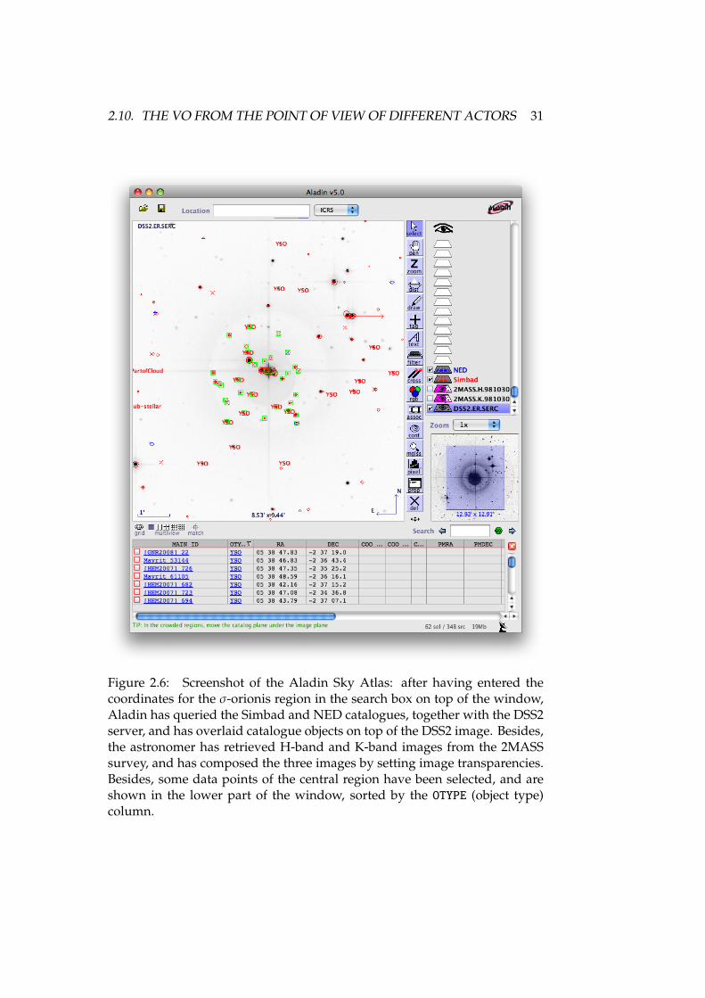
2.10. THE VO FROM THE POINT OF VIEW OF DIFFERENT ACTORS 31
Figure 2.6: Screenshot of the Aladin Sky Atlas: after having entered thecoordinates for the σ-orionis region in the search box on top of the window,Aladin has queried the Simbad and NED catalogues, together with the DSS2server, and has overlaid catalogue objects on top of the DSS2 image. Besides,the astronomer has retrieved H-band and K-band images from the 2MASSsurvey, and has composed the three images by setting image transparencies.Besides, some data points of the central region have been selected, and areshown in the lower part of the window, sorted by the OTYPE (object type)column.
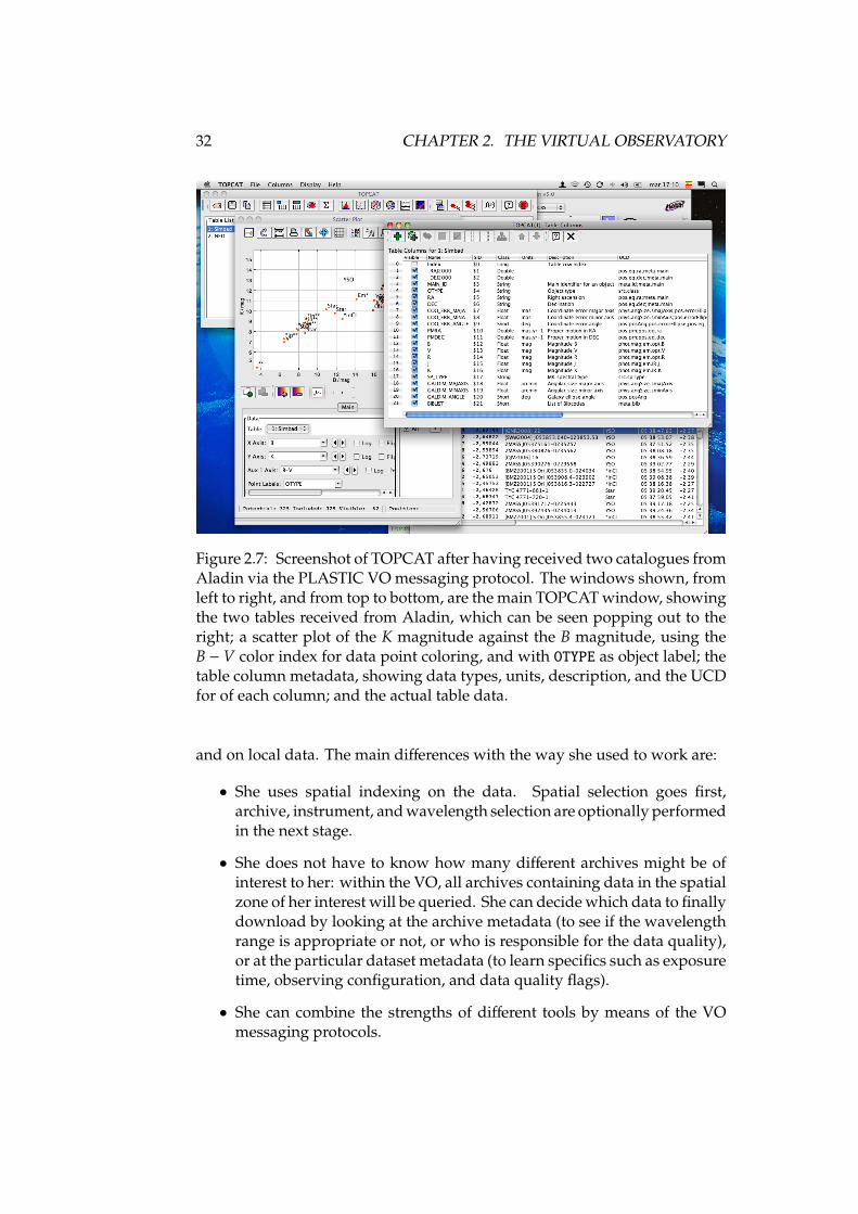
32 CHAPTER 2. THE VIRTUAL OBSERVATORY
Figure 2.7: Screenshot of TOPCAT after having received two catalogues fromAladin via the PLASTIC VO messaging protocol. The windows shown, fromleft to right, and from top to bottom, are the main TOPCAT window, showingthe two tables received from Aladin, which can be seen popping out to theright; a scatter plot of the K magnitude against the B magnitude, using theB − V color index for data point coloring, and with OTYPE as object label; thetable column metadata, showing data types, units, description, and the UCDfor of each column; and the actual table data.
and on local data. The main differences with the way she used to work are:
• She uses spatial indexing on the data. Spatial selection goes first,archive, instrument, and wavelength selection are optionally performedin the next stage.
• She does not have to know how many different archives might be ofinterest to her: within the VO, all archives containing data in the spatialzone of her interest will be queried. She can decide which data to finallydownload by looking at the archive metadata (to see if the wavelengthrange is appropriate or not, or who is responsible for the data quality),or at the particular dataset metadata (to learn specifics such as exposuretime, observing configuration, and data quality flags).
• She can combine the strengths of different tools by means of the VOmessaging protocols.
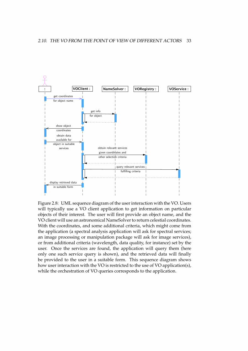
2.10. THE VO FROM THE POINT OF VIEW OF DIFFERENT ACTORS 33
get coordinatesfor object name
get infofor object
show objectcoordinates
obtain dataavailable for
object in suitableservices obtain relevant services
given coordinates andother selection criteria
query relevant servicesfulfilling criteria
display retrieved datain suitable form
Figure 2.8: UML sequence diagram of the user interaction with the VO. Userswill typically use a VO client application to get information on particularobjects of their interest. The user will first provide an object name, and theVO client will use an astronomical NameSolver to return celestial coordinates.With the coordinates, and some additional criteria, which might come fromthe application (a spectral analysis application will ask for spectral services;an image processing or manipulation package will ask for image services),or from additional criteria (wavelength, data quality, for instance) set by theuser. Once the services are found, the application will query them (hereonly one such service query is shown), and the retrieved data will finallybe provided to the user in a suitable form. This sequence diagram showshow user interaction with the VO is restricted to the use of VO application(s),while the orchestration of VO queries corresponds to the application.
34 CHAPTER 2. THE VIRTUAL OBSERVATORY
• She can explore catalogues with higher confidence, because data columnsare fully tagged with standard descriptors (UCDs, Unified Content De-scriptors), which allow automated identification of those datasets.
In other words, she has transparent access to many archives not just froma single tool, but from any tool which is able to query the VO. In marketingterms, any tool sporting a VO-compatible badge.
However, if she wants to exploit the data she has just collected, for instancein order to perform cross-matching between sources, or to create differentcolor diagrams, she needs to know how to find which data columns corre-spond to different astronomical or astrophysical concepts. In other words,she is concerned with data semantics.
The VO from the application developer’s point of view
VO Developers view of the VO arises from what the VO offers for theirapplications. A VO-enabled application, be it brand new or upgraded, can beof two types: data centric or workflow centric. Some data centric applicationscan be scripted to be part of a workflow.
Data centric applications tend to be either data reduction applications orhigh level analysis applications which work on individual datasets at a time.For those applications, the VO is used for:
Finding out interesting datasets That usually means finding archives withdata in the desired wavelength range for certain positions of the sky.
Retrieving candidate datasets Candidate datasets (images, spectra, data cubes)are downloaded one by one, or as a package, to be individually analysedin the local computer.
Local processing One by one processing of the different datasets in orderto obtain scientific grade data products, such as chemical abundance,region temperatures, ionisation states, stellar population age, et cetera.Anything that is obtained from the treatment of the light and the knowl-edge of the physical process at hand.
In this view of the VO, only a few benefits are added over the traditionalastronomer’s workflow, such as providing a single programmatic interfacefor all application to access all archives. That is, the VO provides a uniformdata and metadata access, together with uniform data and metadata format toapplications. Additionally, tools which implement VO messaging protocolsallow the astronomer to use specialised tools for each task, while maintainingalways the benefits of having each application connected to the VO.
On the other hand, workflow centric applications are applications whichwork with large datasets in large batches. For instance, from object types
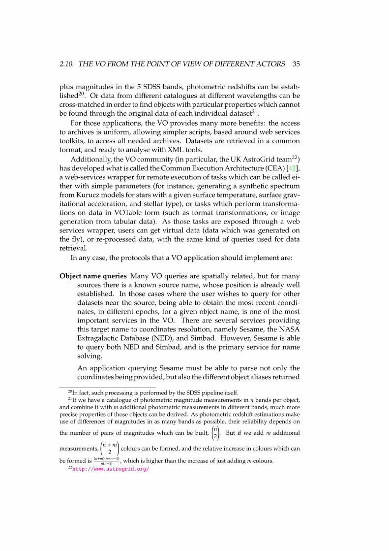
2.10. THE VO FROM THE POINT OF VIEW OF DIFFERENT ACTORS 35
plus magnitudes in the 5 SDSS bands, photometric redshifts can be estab-lished20. Or data from different catalogues at different wavelengths can becross-matched in order to find objects with particular properties which cannotbe found through the original data of each individual dataset21.
For those applications, the VO provides many more benefits: the accessto archives is uniform, allowing simpler scripts, based around web servicestoolkits, to access all needed archives. Datasets are retrieved in a commonformat, and ready to analyse with XML tools.
Additionally, the VO community (in particular, the UK AstroGrid team22)has developed what is called the Common Execution Architecture (CEA) [42],a web-services wrapper for remote execution of tasks which can be called ei-ther with simple parameters (for instance, generating a synthetic spectrumfrom Kurucz models for stars with a given surface temperature, surface grav-itational acceleration, and stellar type), or tasks which perform transforma-tions on data in VOTable form (such as format transformations, or imagegeneration from tabular data). As those tasks are exposed through a webservices wrapper, users can get virtual data (data which was generated onthe fly), or re-processed data, with the same kind of queries used for dataretrieval.
In any case, the protocols that a VO application should implement are:
Object name queries Many VO queries are spatially related, but for manysources there is a known source name, whose position is already wellestablished. In those cases where the user wishes to query for otherdatasets near the source, being able to obtain the most recent coordi-nates, in different epochs, for a given object name, is one of the mostimportant services in the VO. There are several services providingthis target name to coordinates resolution, namely Sesame, the NASAExtragalactic Database (NED), and Simbad. However, Sesame is ableto query both NED and Simbad, and is the primary service for namesolving.
An application querying Sesame must be able to parse not only thecoordinates being provided, but also the different object aliases returned
20In fact, such processing is performed by the SDSS pipeline itself.21If we have a catalogue of photometric magnitude measurements in n bands per object,
and combine it with m additional photometric measurements in different bands, much moreprecise properties of those objects can be derived. As photometric redshift estimations makeuse of differences of magnitudes in as many bands as possible, their reliability depends on
the number of pairs of magnitudes which can be built,(n2
). But if we add m additional
measurements,(n + m
2
)colours can be formed, and the relative increase in colours which can
be formed is (n+m)(n+m−1)n(n−1) , which is higher than the increase of just adding m colours.
22http://www.astrogrid.org/
36 CHAPTER 2. THE VIRTUAL OBSERVATORY
by the service, such as conventional names, coincidental sources atdifferent wavelengths, morphology, redshift, and distance23.
Registry queries Independently of the kind of VO services to be accessed,all applications must be able to query the VO Registry (or registries) sothat they can look for specific services.
Data access queries Once we have coordinates to make our query (or queries),and the application (or the user) has selected entries in the registry thatcan provide useful datasets, the data access protocols relevant to the ap-plication (SCS, SIAP, SSAP, and in the future the TAP) have to be queried,and the returned data (in VOTABLE format) parsed. Appendix D is de-voted to describe the interface to those services, and provides links totheir complete specification.
CEA services If we want our application to take advantage of several remoteVO services, such as those providing data transformation capabilities,mosaicing24, signal processing, or many others running under the CEA,we must implement CEA services calls. The detailed description andspecification of the CEA can be found in [42].
Local messaging services Optionally, the VO interoperability protocols forlocal data interchange and collaboration must be implemented. Thisallows a more modular development of VO tools, letting other applica-tions to pre-process the data, and perform analysis in different ones.
In addition, as VO particular data formats are XML-based, XML manip-ulation toolkits are needed in order to build and interpret VO data, togetherwith FITS processing libraries for applications which must have access to theactual data.
23 For instance, we can query Sesame about M31, and we will learn that it is also known asAndromeda Nebula, Andromeda Galaxy, or simply Andromeda. In specific bands, it corresponds,for instance, with several strong infrared sources from the IRAS catalogue: IRAS F00400+4059and IRAS 00400+4059. Sesame also returns object type information, and simply from queryingSesame we can learn that M31 is an active galaxy of LINER type, with a morphology type of Sb(a spiral galaxy without bars, with packed arms), and at a redshift (z) of −0.001004, meaningthat M31 is, in fact, blueshifted, getting nearer to the Milky Way at a rate of approximately300km/s.
The query which delivers all of this information, in XML format, is:http://cdsws.u-strasbg.fr/axis/services/Sesame?method=sesame&resultType=xi&name=M31
See the CDS Developer’s corner, http://cdsweb.u-strasbg.fr/cdsws.gml, for details onthis and other services.
24Mosaicing is the non-trivial operation of overlaying several astronomical images, withembedded coordinates and resolution information, in order to provide a composition of theoriginal images with a common resolution.
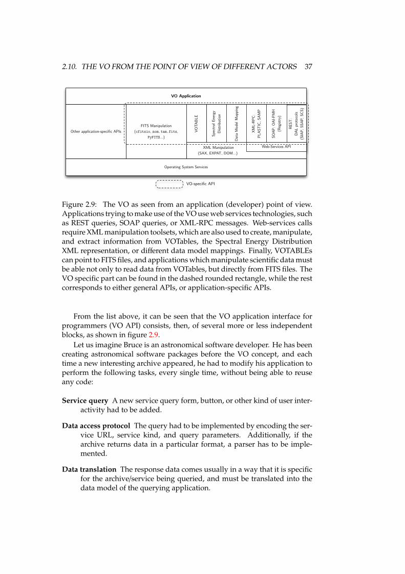
2.10. THE VO FROM THE POINT OF VIEW OF DIFFERENT ACTORS 37
XML Manipulation (SAX, EXPAT, DOM…)
VO Application
FITS Manipulation(cfitsio, nom.tam.fits,
PyFITS…)
VOTA
BLE
Dat
a M
odel
Map
ping
Spec
tral
Ene
rgy
Dist
ribut
ion
Other application-specific APIs
Operating System Services
VO-specific API
REST
:D
AL p
roto
cols
(SIA
P, S
SAP,
SCS
)
SOAP
: OAI
-PM
H(R
egist
ry)
XML-
RPC:
PLAS
TIC,
SAM
P
Web-Services API
Figure 2.9: The VO as seen from an application (developer) point of view.Applications trying to make use of the VO use web services technologies, suchas REST queries, SOAP queries, or XML-RPC messages. Web-services callsrequire XML manipulation toolsets, which are also used to create, manipulate,and extract information from VOTables, the Spectral Energy DistributionXML representation, or different data model mappings. Finally, VOTABLEscan point to FITS files, and applications which manipulate scientific data mustbe able not only to read data from VOTables, but directly from FITS files. TheVO specific part can be found in the dashed rounded rectangle, while the restcorresponds to either general APIs, or application-specific APIs.
From the list above, it can be seen that the VO application interface forprogrammers (VO API) consists, then, of several more or less independentblocks, as shown in figure 2.9.
Let us imagine Bruce is an astronomical software developer. He has beencreating astronomical software packages before the VO concept, and eachtime a new interesting archive appeared, he had to modify his application toperform the following tasks, every single time, without being able to reuseany code:
Service query A new service query form, button, or other kind of user inter-activity had to be added.
Data access protocol The query had to be implemented by encoding the ser-vice URL, service kind, and query parameters. Additionally, if thearchive returns data in a particular format, a parser has to be imple-mented.
Data translation The response data comes usually in a way that it is specificfor the archive/service being queried, and must be translated into thedata model of the querying application.
38 CHAPTER 2. THE VIRTUAL OBSERVATORY
However, all steps above are common for all VO services providing thesame kind of data (catalogues, images, spectra), with the addition of theRegistry query step needed to find out all services providing that kind ofdata, which again has to be implemented only once.
It must be noticed that once the data are in the internal data model of theapplication, it does not matter which was the origin of a particular data set(except for documenting its provenance), and that is the way VO data caninteroperate with non-VO data. An example of application mixing VO withnon-VO data is Aladin: originally Aladin queried different non-VO services,and all VO-services were added as just one additional data source for Aladin.
The VO from the service developer’s point of view
For Bruce, then, the VO is technically rather simple (compared with thearchive access and interface operations already in place in the archive): theservices have to provide access to existing datasets through a web-servicesinterface (most of the time, REST-ful services are used for the VO, except forVO Registry services, which use SOAP queries).
However, the hardest part for VO-services developers is the interfacingbetween the actual data being stored, and the VO data formats, which alsoinclude VO semantics. This is achieved by means of a systematic mappingbetween stored data and data models.
In particular a VO service needs to provide:
VO Service Endpoint(s) A service provider must provide one or more VOservices (delivering images, spectra, or catalogue data). Each differentservice must provide an URL for accessing it, the endpoint. This URLis used to build VO queries by adding parameters to it. Different ser-vices, in the sense that the data they provide corresponds to a differentscientific data product, need to provide different endpoints.
DAL Parser and Query Mechanism The service endpoint parameters haveto be parsed, converted into a query for the internal database (or anyother data access and filtering mechanism), and results obtained. Inshort, the service must comply with the interfaces described in ap-pendix D.
VOTable generation mechanism Once the query has returned results, thesemust be returned into the VOTable format. This includes not only thebuilding of the main tags, which can be considered a wrapper for atabular result, but also the assignment of semantic attributes such asucds and utypes from data model mappings.
Data Model Mapper The VOTable generation mechanism, and the DAL Parser,need a mapping between the data stored in the database and the data
2.11. PRECEDENTS TO THE VO 39
model for the kind of observation being performed. This mapping isused for the filling of the already mentioned semantic attributes.
CEA wrapper A service which provides computing services in the VO en-vironment has to comply with the CEA. A computing service whichwas not built for the VO can integrate into the CEA infrastructure byencapsulating it into a CEA intermediate service (wrapper).
Other task to be eventually performed by the VO Service developer is theendpoint registration. Even when the VO Service can be used as long as itsendpoint is known by any other tool (be it a simple command-line script, ora complete application), new services can only be discovered by tools if theyare registered in a VO Registry.
2.11 Precedents to the VO
The VO infrastructure has taken advantage of already in place systems. Themain precedents are:
The NASA/IPAC Extragalactic Database The NED25 [43] (service acronym),provides online all different catalogues of extragalactic objects ever pub-lished in astronomy. It allows users to perform conesearchs for datacentered on a particular position, and below a certain angular distance,and the results provided the main object positional properties: skycoordinates, distance, relative velocity, object type, morphologycal clas-sification, et cetera, and many other observational parameters, such asgalactic extinction, absolute magnitudes, et cetera.
The Simbad Astronomical Database Simbad26 [44] is an online databasehosted by the Centre de Donées Astronomiques de Strasbourg (CDS),also providing data on different objects outside of our solar system, andthus includes galactic objects. The two databases have a non-emptyintersection, but none is a subset of the other.
The VizieR service for Astronomical Catalogues VizieR27 [45] is a compila-tion of all published astronomical catalogues, classified by wavebandcoverage, space mission if applicable, and/or astrophysical subject.Many astrophysical journals automatically make available in VizieRpositional tables in published articles, and the data is linked to thepublication via the bibcode of the Astrophysics Data System (ADS).
25http://nedwww.ipac.caltech.edu/26http://simbad.u-strasbg.fr/simbad/27http://webviz.u-strasbg.fr/viz-bin/VizieR
40 CHAPTER 2. THE VIRTUAL OBSERVATORY
The SAO/NASA Astrophysics Data System The ADS28 [46] is an online da-tabase containing all bibliographic entries in the fields of Physics andAstrophysics. Entries are proposed by different journal and book pub-lishers, but are also collected from online e-print archives such as thearXiv29. Publications are uniquely identified by a structured code, thebibcode30, which contains details on the publication date, publicationkind, and/or journal, and enough data for unique identification or jour-nal articles. The entries are linked with online versions of the articles,if available, and can be searched by author, words in title or abstract,publication dates, et cetera. VizieR catalogue entries are also consideredpublications by the ADS, with their own bibcode.
These facilities have been federated and linked by means of the bibcode,which allows for the retrieval of publications on any object in Simbad or NED,or for the objects whose data is found in VizieR.
And many observatories, specially space-borne ones, have had onlinearchives from little time after the opening of the Internet and the World WideWeb.
However, all of these services have their own, completely different form-based interfaces, and even when they have started to provide cleaner web-services interfaces, users need to support different query protocols for eachservice, until the VO provided service unification and interoperability tem-plates.
2.12 Comparable activities in other disciplines
We will conclude our introduction of the VO with a selection of other e-science activities which are similar in scope to the Virtual Observatory, butbelong to different scientific fields, or have a different technology base: thedata storage support of data grids, Geographical Information Systems, andthe Bioinformatics Harvester.
Data grids
In e-Science talks, grid technologies tend to come up first and forefront. Evenrepresentatives for e-Science in European countries are typically representedby the National Grid Initiatives, as if e-Science could only be performed viagrid technologies. But the fact is that grid middleware provides some of thecore functionalities that the VO has implemented.
28http://www.adsabs.harvard.edu/29http://arXiv.org/30http://doc.adsabs.harvard.edu/abs_doc/help_pages/bibcodes.html
2.12. COMPARABLE ACTIVITIES IN OTHER DISCIPLINES 41
The definition of grid computing by Ian Foster as a hardware and softwareinfrastructure that provides dependable, consistent, pervasive, and inexpensive ac-cess to high-end computational capabilities [47] is just one part of the VirtualObservatory.
But computation is just a fraction of the VO. In fact, the VO can be moreclosely identified with a data grid [48]: an extension of the grid protocolsin order to create a standard for distributed data storage, data identifica-tion, and metadata management which can integrate archives from differentdisciplines.
In the VO, the data grid exists via the data access protocols, and the stan-dardisation of metadata. A version of the VO can exist implemented on topof grid protocols, but web-services technology was chosen instead in order tominimise the cost of entry for participant institutions/research groups: web-services technology is easier to implement and deploy, both for servers andspecially for clients, and it was very important to be able to have a productiveVO that could engage the community.
In the future, however, the VO can move more towards a grid technologyfoundation, when the computing needs overcome the data needs, and theVO metadata standards are complete. In the meantime, VO protocols are astechnology agnostic as possible. For instance, the IVOA is working in a dis-tributed file system for VO tools, reminiscent of grid data storage pools, withVO specific metadata and implementation independent (it can use WebDAV,NFS, GridFTP, or any other supporting protocol), called VOSpace [49].
Geographical Information Systems
There are many similarities between the VO and Geographical InformationSystems (GIS):
Coordinate system based Both for GIS and the VO, coordinates are one ofthe main indices on data. Finding data nearby a particular coordinate isalso a common feature, and the retrieval of nearby candidates cannot bebased on floating point differences, as it would become computationallycostly. The solution for fast operation of coordinate-based data retrievalis the hierarchical partitioning of the search space using, for instance,techniques such as the Hierarchical Triangular Mesh [50] or the QuadTree Cube [51].
Object to coordinates resolution Also common to both problem domains isthe need to obtain coordinates for a particular object whose only knownproperty is the name. In astronomy such needs are typically handledby the Simbad or NED services, while different GIS systems will usedifferent local or remote databases for obtaining the coordinates.
42 CHAPTER 2. THE VIRTUAL OBSERVATORY
Use of metadata GIS objects are primarily graphs31 with geographical coor-dinates attached to both connections and nodes. But those curves rep-resent roads, buildings, water and gas distribution pipes, agriculturalplantations, et cetera, and each object kind has its own set of metadata,in the same way VO data uses metadata to establish object kind, andinformation kind.
The main difference between the VO and GIS systems is that for the VOthere is a strong standardisation force mandating which data formats to use,and there is usually no restriction in data usage32, and interoperation andnetworking is a key concept in system design, while it is not so for GIS.
However, some GIS systems such as Google Earth33 have started to showthe potential of having a common geographical description format combinedwith the distributed dataset creation and distribution: GIS data, both imagesand object catalogues with metadata can be updated on the data server, andall clients access updated data from then on.
It is remarkable in this context that Google Earth has evolved to includeGoogle Sky, which demonstrates the similar nature of GIS and VO systemswhen the distributed, interoperable data access is taken into account.
Bioinformatic Harvester
The Bioinformatic Harvester34 (BioH) is a bioinformatic meta search engineat KIT Karlsruhe Institute of Technology for genes and protein-associatedinformation. It queries data from more than 35 bioinformatic sites, whichallows for searches in the genome and proteins of several animals of the mostimportant sequenced animals —among them humans, rats, or the drosophila(fruit fly)— or on the complete collection.
The similarities with the VO lie in the distributed nature of the integratedsystems, but the similarities end there:
• the BioH does not use a unified, standardised protocol for harvestingthe data available in the different resources; instead, it uses a custombuilt harvesting engine for each collection.
• there is only one entry point to the Harvester, and there is no publicservice access entry point for external applications.
We can see the BioH as bioinformatic equivalent of the state of affairs inastronomy prior to the VO: similar to the joint ADS and VizieR systems.
31In the mathematical sense: a set of directed connections between sets of nodes.32After all, astrophysical data tend not to be of immediate value for entrepreneurial use.33http://earth.google.com/34http://harvester.fzk.de/harvester/
Part II
Radio astronomical archives inthe VO
43

Chapter 3
Introduction
Due to the more abstract nature of radio astronomical observations, thereare less astronomers and observatories providing radio astronomical data.However, as multi-wavelength studies become more and more commonplacein astrophysics, and are essential for studies such as the one being carriedout within the AMIGA group, being able to access radio astronomical databecomes of the utmost importance.
There are few radio astronomical observatories with proper archives (mostof them provide logbooks, or observation registries, if that much), so provid-ing VO-compatible radio astronomical archives is a valuable contributionto the community both because of the availability of the archive, and thepossibility of using VO-tools to access it.
For existing archives, the data model of the archive itself does not usuallymatch the data model of the VO, mainly due to the difference in scope: archivedata models reflect the data origin, and are built to answer the queries ofengineers, commissioning scientists and scientists; VO data models, on theother hand, are built to describe observations so that the description is enoughfor astronomers, or computer queries, to assess the usefulness of a particularpiece of data.
For a new archive, however, the internal archive data model can be builtby mirroring VO data models, while adding non-VO information so that allneeds can be covered.
In this part, we will describe the RADAMS, a data model for single-dishradio astronomical archives reflecting existing IVOA data models, but whichat the same time provides definitions and proposals for modelling additionalobservational aspects. We will use this data model for the building of theIRAM 30m and DSS-63 archives, which will be shown Part IV.
In addition, some parts of the RADAMS will be used in the developmentof the MOVOIR, a modular VO interface and API to the VO, which will bedescribed in Part III.
We will start by introducing which are the existing IVOA data models
45

46 CHAPTER 3. INTRODUCTION
in chapter 4, and then we will evaluate parts of those models to create theRADAMS (Radio Astronomical DAta Model for Single-dish observations) inchapter 5. Chapter 6 explains how the RADAMS can be used to charac-terise astronomical observations, and the following chapters explore in detailwhich are the missing parts in IVOA data models which are needed for theRADAMS: Curation, Packaging and Policy are specified in chapter 7, whiledata provenance in e-science is reviewed in chapter 8, and the lessons learnedapplied to RADAMS’ Provenance in chapter 9.

Chapter 4
Data modelling in the VO
The interoperability of tools and archives in the VO is only achievable bystandardising the way datasets are accessed, and how the scientific data theycontain is described. The first part is solved by means of standard accessprotocols, while the latter needs the development of suitable data models.
A data model can be defined as a complete description of the set of entitiesneeded for information storage in a particular field, which specifies both thedata being stored, and the relationships between them.
In this way, it can also be seen as the framework in which questions aboutthe data (and metadata) ca be posed: only questions which can be answeredregarding the information AND relationships encoded in the data model canbe answered within the VO framework. And considered this way, a uniform,interoperable observation data model can be mapped into a uniform set ofquestions which can be answered within the VO.
Two main classes of data models are typically considered:
Domain data models These are high-level descriptions of the entities to betaken into account in order to fully implement a data model. Particularattributes of the data entities involved are not set, except for thoseneeded for establishing the relationship between entities.
Implementation model Implementation-dependent description of the par-ticular entities and attributes to be actually stored.
VO data models need to be a mixture of the model types above: for thedata models to be used across observations with different instruments, andwith different scientific objectives in mind, a high-level description is needed.In addition, VO data models affect how data from observatories’ archivesare exposed through VO services, not necessarily to the way such data arestored by the archive. However, there are particular attributes that need aprecise description in order for the model to be useful and, and to be able
47
48 CHAPTER 4. DATA MODELLING IN THE VO
to implement it, so VO data models need to fix the kind of metadata theysupport.
Within the VO, data models apply not only directly to the scientific data,but to the metadata describing them. As the way to structure informationdepends on the application domain, VO data models describe astronomicaldatasets in a way that is as instrument independent as possible, to ensurethat the same description can be used for data with different origins. Usersmust also be able to query those data models to be able to find datasets whichcomply with certain properties.
4.1 Elements of a data model
When defining a VO data model, we have to specify:
Entities Being the data model building blocks, they group related attributeswithin a data model. They can be mapped to Classes in Object-OrientedProgramming (OOP), or Elements in XML.
Fields They are the actual data elements of the model. They map to Attributesin OOP, and they can be mapped to Attributes or to Elements withoutchildren in XML.
Relationships The different entities and fields have hierarchical or relationalrelationships: an observation projects has projected observations, andall entities which share a common project ID are related, for instance.For the data model to be uniquely defined those relationships must bemade explicit.
Cardinalities The number of object instances allowed as part of a relation-ship. It is specified as a range of valid number of entities. For instance,an observation can be related to any number of data files, but it needs tobe related at least with one, meaning that the cardinality of the Obser-vation to Data files relationship would be specified as 1..*. For objectswhich can appear any number of times, including none, the cardinalityis expressed as 0..*. Objects which are optional, but if present can appearjust once have their cardinality expressed as 0..1, and so on.
Data types For computers to be able to correctly interpret a data streama Data type needs to be specified. For instance, object IDs could beIntegers, but they are normally textual, so String data must be used. Wecould consider the restrictions which can be defined for complex datatypes in XML as part of the data typing.
Units No physical quantity can be specified without providing its units.Physical-data related Fields need Units to be specified, or Units have to
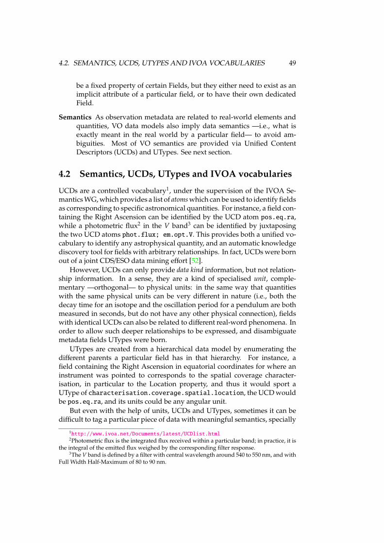
4.2. SEMANTICS, UCDS, UTYPES AND IVOA VOCABULARIES 49
be a fixed property of certain Fields, but they either need to exist as animplicit attribute of a particular field, or to have their own dedicatedField.
Semantics As observation metadata are related to real-world elements andquantities, VO data models also imply data semantics —i.e., what isexactly meant in the real world by a particular field— to avoid am-biguities. Most of VO semantics are provided via Unified ContentDescriptors (UCDs) and UTypes. See next section.
4.2 Semantics, UCDs, UTypes and IVOA vocabularies
UCDs are a controlled vocabulary1, under the supervision of the IVOA Se-mantics WG, which provides a list of atoms which can be used to identify fieldsas corresponding to specific astronomical quantities. For instance, a field con-taining the Right Ascension can be identified by the UCD atom pos.eq.ra,while a photometric flux2 in the V band3 can be identified by juxtaposingthe two UCD atoms phot.flux; em.opt.V. This provides both a unified vo-cabulary to identify any astrophysical quantity, and an automatic knowledgediscovery tool for fields with arbitrary relationships. In fact, UCDs were bornout of a joint CDS/ESO data mining effort [52].
However, UCDs can only provide data kind information, but not relation-ship information. In a sense, they are a kind of specialised unit, comple-mentary —orthogonal— to physical units: in the same way that quantitieswith the same physical units can be very different in nature (i.e., both thedecay time for an isotope and the oscillation period for a pendulum are bothmeasured in seconds, but do not have any other physical connection), fieldswith identical UCDs can also be related to different real-word phenomena. Inorder to allow such deeper relationships to be expressed, and disambiguatemetadata fields UTypes were born.
UTypes are created from a hierarchical data model by enumerating thedifferent parents a particular field has in that hierarchy. For instance, afield containing the Right Ascension in equatorial coordinates for where aninstrument was pointed to corresponds to the spatial coverage character-isation, in particular to the Location property, and thus it would sport aUType of characterisation.coverage.spatial.location, the UCD wouldbe pos.eq.ra, and its units could be any angular unit.
But even with the help of units, UCDs and UTypes, sometimes it can bedifficult to tag a particular piece of data with meaningful semantics, specially
1http://www.ivoa.net/Documents/latest/UCDlist.html2Photometric flux is the integrated flux received within a particular band; in practice, it is
the integral of the emitted flux weighed by the corresponding filter response.3The V band is defined by a filter with central wavelength around 540 to 550 nm, and with
Full Width Half-Maximum of 80 to 90 nm.

50 CHAPTER 4. DATA MODELLING IN THE VO
for data which does not have a direct place in a VO data model. For thatwe can borrow techniques from the Semantic Web (an effort for providingweb documents with semantics, so that, for instance, a table of camera pricescan be tagged so that software tools can identify in it prices, if possiblebelonging to digital cameras, even to particular brands), and provide oneor more standardised astronomical vocabularies. The IVOA Semantics WG4
has started recreating controlled vocabularies such as UCDs in Semantic Webform, and even the IAU thesaurus has been recreated in that way [53]. We willshow how we are using them in the IRAM 30m archive in order to providesemantics to data related to antenna engineering terms.
4.3 Role of data models in the VO
We can identify in the VO four different phases, and we can see that in all ofthem data models play a central role:
Discovery Datasets available in the VO have to be discoverable for themto appear automatically in VO tools. The VO Registry holds data forexisting datasets so that they can be easily discovered. For this phase tobe standardised, we need: data models for Resource metadata (ResDM),were a Resource is either a data provider, an authority, or a data service;a data model for Space-Time Coordinates (STC), so that coordinate-based, region-based or time-based searches can be performed; and adata model for dataset Characterisation (CharDM), so that searches onphysical or instrumental properties are possible. In addition, the UCDand IVOA thesaurus (IVOAT) are relevant in this phase.
Evaluation Datasets have to be evaluated in order to assess their applicabilityto the kind of analysis we might wish to perform; for instance, in orderto do image mosaicing we need a certain coordinate overlap, and inorder to do image stacking we need an almost complete overlap, andcomparable resolutions. The main data model involved in this phase isthe CharDM.
Data Access There is an implicit data model in the IVOA data access proto-cols, the Data Access Layer (DAL), which is centred on targets (coor-dinates with tolerances/search radii), and uses several properties fromthe CharDM, such as the Coverage in several axes, and a streamlinedform of the STC.
Transformation When creating a new dataset, or transforming an existingone, a new CharDM instance needs to be created, one that characterisesthe union of the participating datasets. If the transformed data set
4http://www.ivoa.net/cgi-bin/twiki/bin/view/IVOA/IvoaSemantics
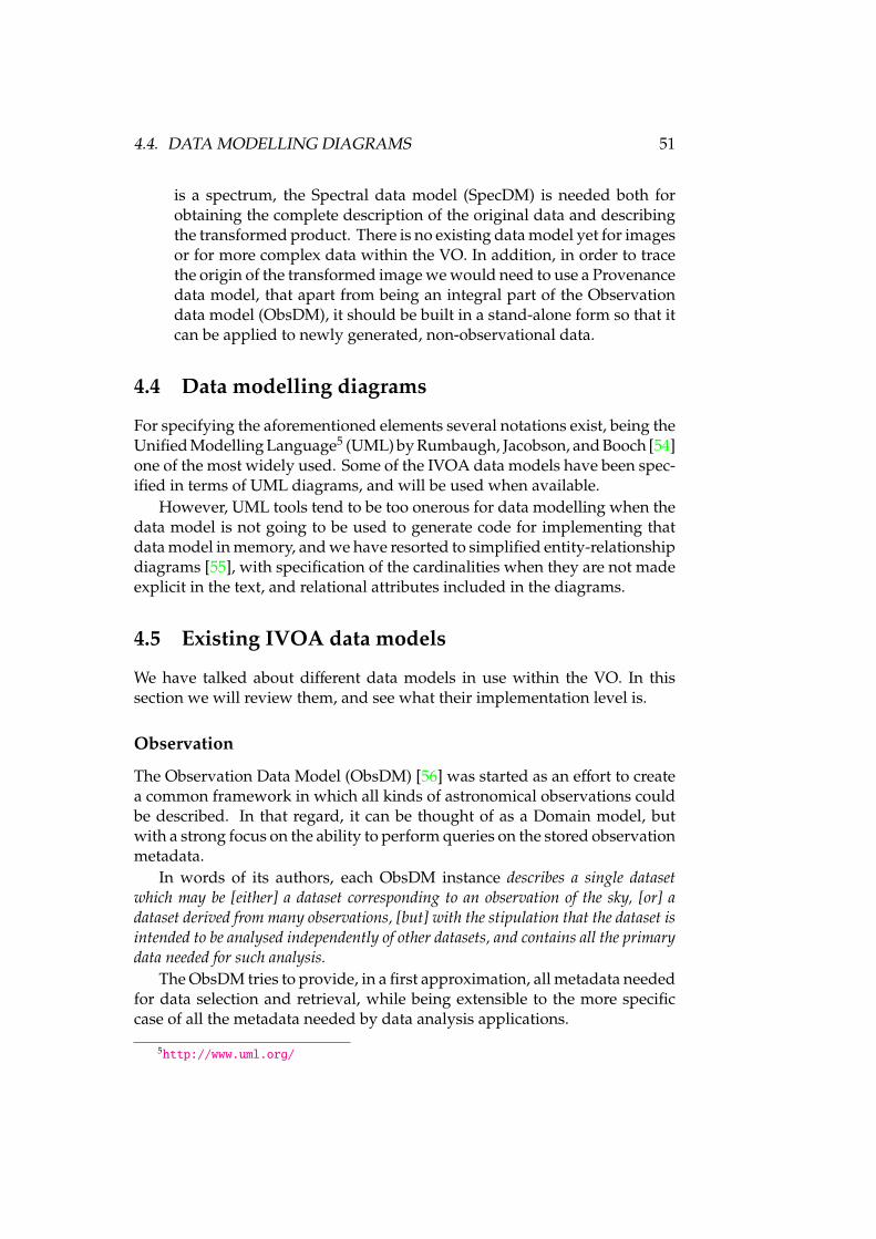
4.4. DATA MODELLING DIAGRAMS 51
is a spectrum, the Spectral data model (SpecDM) is needed both forobtaining the complete description of the original data and describingthe transformed product. There is no existing data model yet for imagesor for more complex data within the VO. In addition, in order to tracethe origin of the transformed image we would need to use a Provenancedata model, that apart from being an integral part of the Observationdata model (ObsDM), it should be built in a stand-alone form so that itcan be applied to newly generated, non-observational data.
4.4 Data modelling diagrams
For specifying the aforementioned elements several notations exist, being theUnified Modelling Language5 (UML) by Rumbaugh, Jacobson, and Booch [54]one of the most widely used. Some of the IVOA data models have been spec-ified in terms of UML diagrams, and will be used when available.
However, UML tools tend to be too onerous for data modelling when thedata model is not going to be used to generate code for implementing thatdata model in memory, and we have resorted to simplified entity-relationshipdiagrams [55], with specification of the cardinalities when they are not madeexplicit in the text, and relational attributes included in the diagrams.
4.5 Existing IVOA data models
We have talked about different data models in use within the VO. In thissection we will review them, and see what their implementation level is.
Observation
The Observation Data Model (ObsDM) [56] was started as an effort to createa common framework in which all kinds of astronomical observations couldbe described. In that regard, it can be thought of as a Domain model, butwith a strong focus on the ability to perform queries on the stored observationmetadata.
In words of its authors, each ObsDM instance describes a single datasetwhich may be [either] a dataset corresponding to an observation of the sky, [or] adataset derived from many observations, [but] with the stipulation that the dataset isintended to be analysed independently of other datasets, and contains all the primarydata needed for such analysis.
The ObsDM tries to provide, in a first approximation, all metadata neededfor data selection and retrieval, while being extensible to the more specificcase of all the metadata needed by data analysis applications.
5http://www.uml.org/
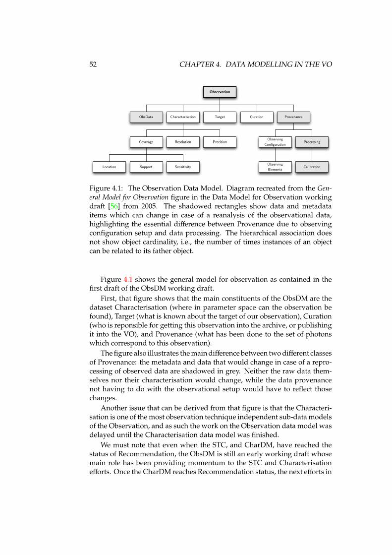
52 CHAPTER 4. DATA MODELLING IN THE VO
Observation
ObsData Characterisation Target
Coverage
Location Support Sensitivity
Resolution Precision
Curation Provenance
Observing Configuration
Observing Elements
Processing
Calibration
Figure 4.1: The Observation Data Model. Diagram recreated from the Gen-eral Model for Observation figure in the Data Model for Observation workingdraft [56] from 2005. The shadowed rectangles show data and metadataitems which can change in case of a reanalysis of the observational data,highlighting the essential difference between Provenance due to observingconfiguration setup and data processing. The hierarchical association doesnot show object cardinality, i.e., the number of times instances of an objectcan be related to its father object.
Figure 4.1 shows the general model for observation as contained in thefirst draft of the ObsDM working draft.
First, that figure shows that the main constituents of the ObsDM are thedataset Characterisation (where in parameter space can the observation befound), Target (what is known about the target of our observation), Curation(who is reponsible for getting this observation into the archive, or publishingit into the VO), and Provenance (what has been done to the set of photonswhich correspond to this observation).
The figure also illustrates the main difference between two different classesof Provenance: the metadata and data that would change in case of a repro-cessing of observed data are shadowed in grey. Neither the raw data them-selves nor their characterisation would change, while the data provenancenot having to do with the observational setup would have to reflect thosechanges.
Another issue that can be derived from that figure is that the Characteri-sation is one of the most observation technique independent sub-data modelsof the Observation, and as such the work on the Observation data model wasdelayed until the Characterisation data model was finished.
We must note that even when the STC, and CharDM, have reached thestatus of Recommendation, the ObsDM is still an early working draft whosemain role has been providing momentum to the STC and Characterisationefforts. Once the CharDM reaches Recommendation status, the next efforts in
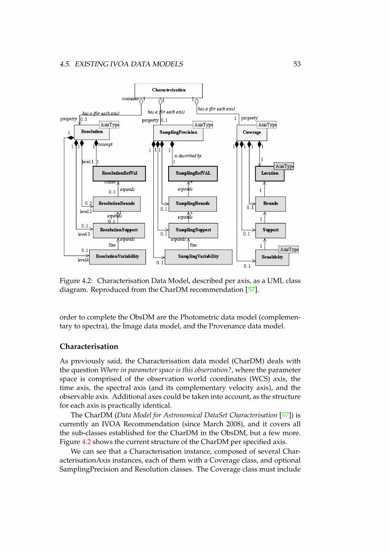
4.5. EXISTING IVOA DATA MODELS 53
Figure 4: The layered structure of Characterisation: This diagram synthe-sises the Property/Axis/Layer approach. The concepts are represented in yel-low. The coarse description is designed by the first level (blue boxes), while thepale blue ones represent the complementary metadata. The Bounds, Supportand Sensitivity classes are nested levels of detail to add knowledge about theCoverage of an Observation. Symmetrically, Resolution and Sampling mayalso have the 4-level structure of description. The complete Characterisa-tion for one observation is obtained by filling the tree for each relevant axis:spatial, spectral, temporal, etc.
17
Figure 4.2: Characterisation Data Model, described per axis, as a UML classdiagram. Reproduced from the CharDM recommendation [57].
order to complete the ObsDM are the Photometric data model (complemen-tary to spectra), the Image data model, and the Provenance data model.
Characterisation
As previously said, the Characterisation data model (CharDM) deals withthe question Where in parameter space is this observation?, where the parameterspace is comprised of the observation world coordinates (WCS) axis, thetime axis, the spectral axis (and its complementary velocity axis), and theobservable axis. Additional axes could be taken into account, as the structurefor each axis is practically identical.
The CharDM (Data Model for Astronomical DataSet Characterisation [57]) iscurrently an IVOA Recommendation (since March 2008), and it covers allthe sub-classes established for the CharDM in the ObsDM, but a few more.Figure 4.2 shows the current structure of the CharDM per specified axis.
We can see that a Characterisation instance, composed of several Char-acterisationAxis instances, each of them with a Coverage class, and optionalSamplingPrecision and Resolution classes. The Coverage class must include
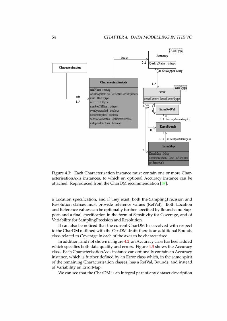
54 CHAPTER 4. DATA MODELLING IN THE VO
Figure 5: This class diagram illustrates the CharacterisationAxis class andits relationship with the Accuracy class, which encompasses various types oferrors such as systematic or statistical.
20
Figure 4.3: Each Characterisation instance must contain one or more Char-acterisationAxis instances, to which an optional Accuracy instance can beattached. Reproduced from the CharDM recommendation [57].
a Location specification, and if they exist, both the SamplingPrecision andResolution classes must provide reference values (RefVal). Both Locationand Reference values can be optionally further specified by Bounds and Sup-port, and a final specification in the form of Sensitivity for Coverage, and ofVariability for SamplingPrecision and Resolution.
It can also be noticed that the current CharDM has evolved with respectto the CharDM outlined with the ObsDM draft: there is an additional Boundsclass related to Coverage in each of the axes to be characterised.
In addition, and not shown in figure 4.2, an Accuracy class has been addedwhich specifies both data quality and errors. Figure 4.3 shows the Accuracyclass. Each CharacterisationAxis instance can optionally contain an Accuracyinstance, which is further defined by an Error class which, in the same spiritof the remaining Characterisation classes, has a RefVal, Bounds, and insteadof Variability an ErrorMap.
We can see that the CharDM is an integral part of any dataset description
4.5. EXISTING IVOA DATA MODELS 55
to be made, and is as observation independent as possible. Indeed, theCharDM is also used within the VODataResource service description in orderto characterise whole archives, or particular subsets of interest in the Registry.
Space and Time Coordinates
The Space and Time Coordinates data model [58] (STC) was created in orderto have a systematic way of specifying different coordinate systems withinthe VO.
While initially the supported coordinate systems for VOTables and dataaccess protocols have been Equatorial, with the possibility to further specifyan epoch, and the IAU has gone a step further with the approval of theInternational Coordinate Reference System (ICRS), equatorial coordinates arenot the natural system for several astronomical disciplines, such as SolarSystem science, or Galactic studies.
The STC is both a data model (it specifies quantities and relationships),but also incorporates two ways of expressing serialisations of data model in-stances: STC-X, an XML-based STC serialisation, and STC-S, which is string-based and more compact and human readable, for use in data models wherean XML payload cannot be delivered, or ease of writing is desirable.
Within the VO there are three places where the STC can be used: dataaccess queries, Characterisation of observation Coverage in both the Spatialand Temporal axes, and the Object to Position resolution. However, for mostof the existing VO services, either J2000 or ICRS equatorial coordinates areassumed.
The complexity of the STC stems from the very different coordinate sys-tems used in astronomy, and the aim to be an all-encompassing effort. Aglimpse of its complexity can be seen in figure 4.4, which shows the mostbasic STC entities6.
Even when the STC is an IVOA Recommendation, is subject to analysisfor better embedding in other data models (see the Spectrum case in thefollowing section), and tools for creating/analysing STC entities are still to bedeveloped.
Spectrum
The Spectrum data model (SpecDM) is different from the data models abovein that it describes a particular data product, and not just a generic observationor an observation set.
Figure 4.5 shows the high-level overview of the Spectrum data model.Compared with the ObsDM, —see figure 4.1— and the CharDM —see fig-ure 4.2—, it can be seen that the Spectral data model is based on the ObsDM,
6And on the STC Recommendation length, which runs at 109 pages.
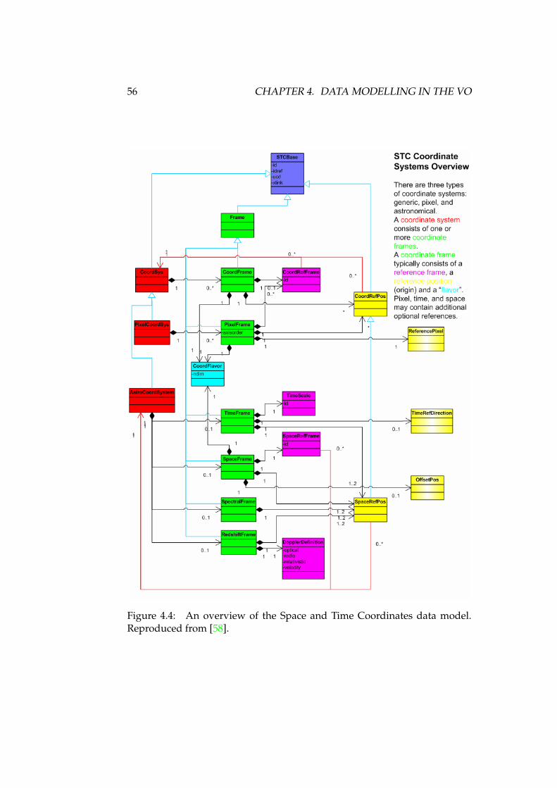
56 CHAPTER 4. DATA MODELLING IN THE VO
!"#$%&'()('($*+,$'-&$./$
0112341351"46754711$ $ 8(9&$::$+*$41;$
Figure 4.4: An overview of the Space and Time Coordinates data model.Reproduced from [58].
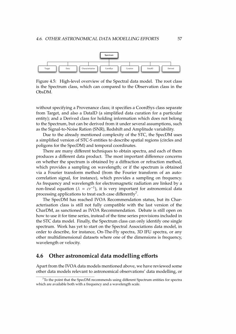
4.6. OTHER ASTRONOMICAL DATA MODELLING EFFORTS 57
Spectrum
Target Data Characterisation CoordSys Curation DataID Derived
Figure 4.5: High-level overview of the Spectral data model. The root classis the Spectrum class, which can compared to the Observation class in theObsDM.
without specifying a Provenance class; it specifies a CoordSys class separatefrom Target, and also a DataID (a simplified data curation for a particularentity); and a Derived class for holding information which does not belongto the Spectrum, but can be derived from it under several assumptions, suchas the Signal-to-Noise Ration (SNR), Redshift and Amplitude variability.
Due to the already mentioned complexity of the STC, the SpecDM usesa simplified version of STC-S entities to describe spatial regions (circles andpoligons for the SpecDM) and temporal coordinates.
There are many different techniques to obtain spectra, and each of themproduces a different data product. The most important difference concernson whether the spectrum is obtained by a diffraction or refraction method,which provides a sampling on wavelength; or if the spectrum is obtainedvia a Fourier transform method (from the Fourier transform of an auto-correlation signal, for instance), which provides a sampling on frequency.As frequency and wavelength for electromagnetic radiation are linked by anon-lineal equation (λ = cν−1), it is very important for astronomical dataprocessing applications to treat each case differently7.
The SpecDM has reached IVOA Recommendation status, but its Char-acterisation class is still not fully compatible with the last version of theCharDM, as sanctioned as IVOA Recommendation. Debate is still open onhow to use it for time series, instead of the time series provisions included inthe STC data model. Finally, the Spectrum class can only identify one singlespectrum. Work has yet to start on the Spectral Associations data model, inorder to describe, for instance, On-The-Fly spectra, 3D IFU spectra, or anyother multidimensional datasets where one of the dimensions is frequency,wavelength or velocity.
4.6 Other astronomical data modelling efforts
Apart from the IVOA data models mentioned above, we have reviewed someother data models relevant to astronomical observations’ data modelling, or
7To the point that the SpecDM recommends using different Spectrum entities for spectrawhich are available both with a frequency and a wavelength scale.
58 CHAPTER 4. DATA MODELLING IN THE VO
data modelling for radio astronomical archives.The only IVOA Note on radio astronomy data prior to the publication
of the RADAMS was the Data model for Raw Radio Telescope by Lamb andPower [59].
Many aspects of our work —specially controlled vocabularies, and theextensibility to interferometry— were initially based upon this model.
Other models reviewed include the data model used for publication ofthe Australian Telescope Compact Array (ATCA) [60] archive8, the scien-tific archive domain model of the National Optical Astronomy Observatory(NOAO) [61] archives9, and the ALMA Science Data Model10 [62].
A special mention is made of the MPEG-7 and MPEG-21 overview doc-uments [63, 64], available in web-page form at http://www.chiariglione.org/, used as the basis for our Policy and Curation sub-models.
4.7 Conclusions
Within the VO, data to be delivered must be described in the most completepossible way so that automated selection and manipulation tools can relyon that description in order to manipulate, select, and ultimately provideunderstanding of the described data.
Both the data themselves and the metadata need to conform to a com-mon data model, in order to make interoperability between different systemspossible. Those data models are governed by the IVOA DM WG.
The only observation-related data model already in Recommendationstage is the SpecDM. The other data models having reached Recommendationstatus are the STC data model, and the CharDM.
The SpecDM shows that it is possible to use the ObsDM as a template tocreate an observation-specific data model, and both the CharDM and the STChave shown their modularity in order to be embedded in other data models.However, STC entities are usually simplified before being properly used.
In order to create a complete VO-compliant data model which can hold allkinds of radio observations from different single-dish observatories we willprovide, then:
Compatibility with existing and/or proposed data models Any VO-compli-ant data model should make use of existing and recommended IVOAdata models, and should try to fit themselves in the data model thatcovers the most the kind of desired data model application.
8http://atoa.atnf.csiro.au/9http://archive.noao.edu/nsa/
10http://aramis.obspm.fr/~alma/ASDM/ASDMEntities/
4.7. CONCLUSIONS 59
Use of existing data models in comparable e-Science disciplines The VirtualObservatory is one example of an e-Science based discipline: the mainsuccess of the VO comes from the federation of disperse datasets, andtheir aggregation through network access protocols. As such, it wouldbe wise to make use of the existing e-Science middleware and conven-tions for non astronomy-specific parts of the system.
Support for spectral associations The SpecDM provides support for spectralmeasurements, but there is no way to relate spectra taken from On-The-Fly observations, or spectra extracted from a radio data cube, or mapsof continuum measurements. This support is added to the RADAMSby combining the CharDM and Packaging.
Specification of missing classes The ObsDM proposed classes for dealingwith data access Policies, data Provenance, and data Packaging, whilethe CharDM proposed a Sensitivity class. A data model for radio as-tronomical observations would need to provide definitions for suchclasses.
Support for radio astronomical observing modes There are widely differ-ent observing modes in radio astronomical, single dish, observatories.A VO data model for them would have to support them.
Extensibility for radio interferometric observations Most of the data modeldetails can be generalised for radio interferometric observations, andwhere possible the way to extend the data model in order to supportinterferometric observations is made explicit.
We will address these requirements in the following chapters.

Chapter 5
RADAMS: a RadioAstronomical DAta Model forSingle-dish radio telescopes
In the past chapters we have been making emphasis on how the VO worksby providing common data access protocols, common data formats for in-formation interchange, and a common data model for expressing, withinthe constraints of the data model and data access protocols of the VO, thedescription of observational data.
In particular, in the previous chapter we have shown the general frame-work proposed by the IVOA for describing whole observations, characteris-ing the parameter space occupied by them, and using a specific format/datamodel for indicating space and time restrictions. We have also seen thatthe Observation data model is not complete, while the CharDM and STCare mature enough to have been granted the IVOA Recommendation status.However, they have never been applied to radio astronomical archives, andhave never been used as the basis for a radio astronomical archive.
In this chapter we will try to answer the question: How to architecture aVO-compatible radio astronomical archive?, and for that we will use the outlinedObsDM as a foundation in order to create a complete data model for radioastronomical observations which can be used both for the development ofsingle-dish radio astronomical archives, enhancing the existing IVOA Obser-vation data model at the same time.
5.1 Basic requirements of astronomical archives
We will start stating the obvious: a radio astronomical online archive hasto provide a way for astronomers to find and retrieve radio astronomicalobservations. The most simple incarnation of such an archive would include
61
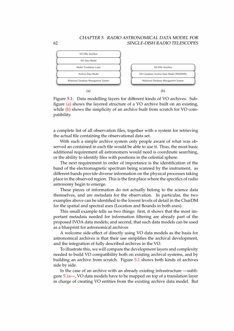
62CHAPTER 5. RADIO ASTRONOMICAL DATA MODEL FOR
SINGLE-DISH RADIO TELESCOPES
VO Data Model
VO DAL Interface
Model Translation Layer
Archive Data Model
Relational Database Management System
(a)
VO-Compliant Archive Data Model (RADAMS)
VO DAL Interface
Relational Database Management System
(b)
Figure 5.1: Data modelling layers for different kinds of VO archives. Sub-figure (a) shows the layered structure of a VO archive built on an existing,while (b) shows the simplicity of an archive built from scratch for VO com-patibility.
a complete list of all observation files, together with a system for retrievingthe actual file containing the observational data set.
With such a simple archive system only people aware of what was ob-served an contained in each file would be able to use it. Thus, the most basicadditional requirement all astronomers would need is coordinate searching,or the ability to identify files with positions in the celestial sphere.
The next requirement in order of importance is the identification of theband of the electromagnetic spectrum being scanned by the instrument, asdifferent bands provide diverse information on the physical processes takingplace in the observed region. This is the first place where the specifics of radioastronomy begin to emerge.
These pieces of information do not actually belong to the science datathemselves, and are metadata for the observation. In particular, the twoexamples above can be identified to the lowest levels of detail in the CharDMfor the spatial and spectral axes (Location and Bounds in both axes).
This small example tells us two things: first, it shows that the most im-portant metadata needed for information filtering are already part of theproposed IVOA data models; and second, that such data models can be usedas a blueprint for astronomical archives
A welcome side-effect of directly using VO data models as the basis forastronomical archives is that their use simplifies the archival development,and the integration of fully described archives in the VO.
To illustrate this, we will compare the development layers and complexityneeded to build VO compatibility both on existing archival systems, and bybuilding an archive from scratch. Figure 5.1 shows both kinds of archivesside by side.
In the case of an archive with an already existing infrastructure —subfi-gure 5.1a—, VO data models have to be mapped on top of a translation layerin charge of creating VO entities from the existing archive data model. But
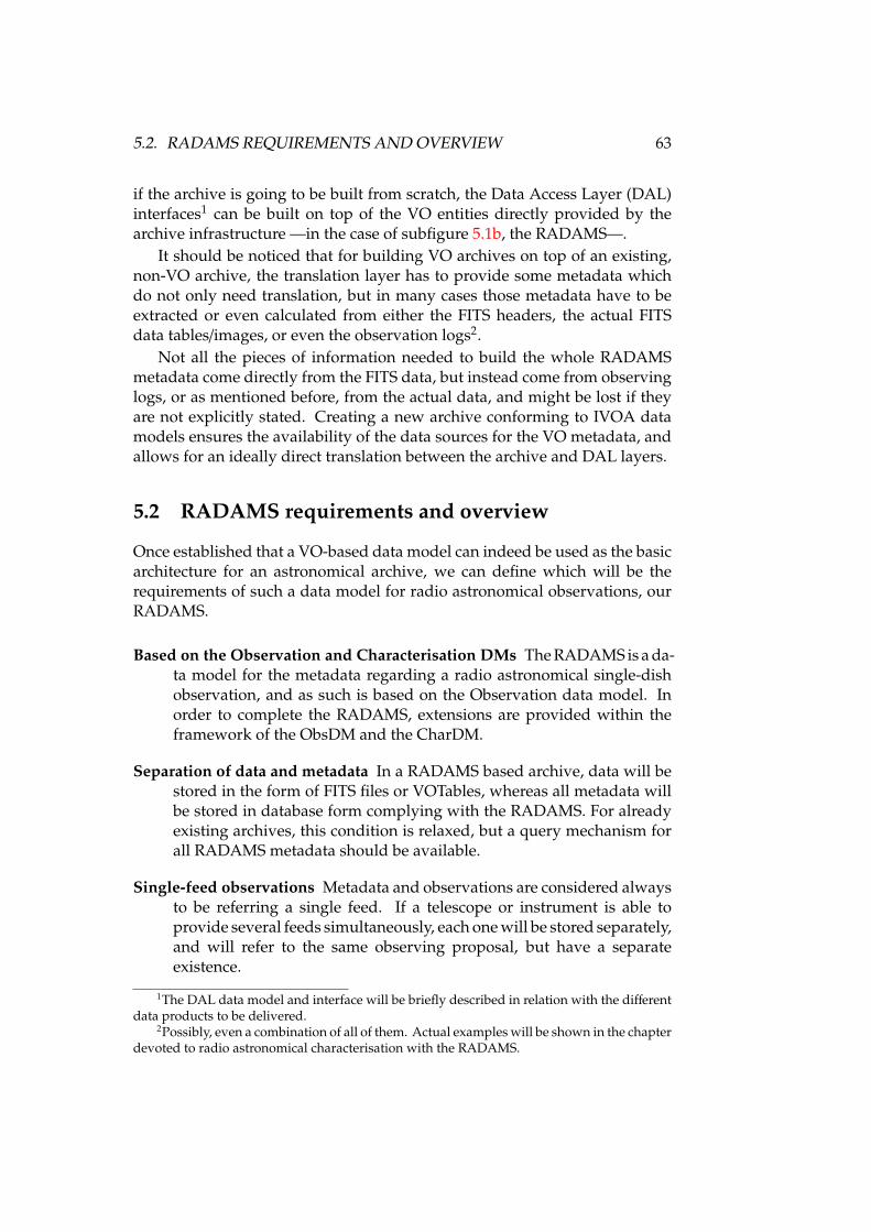
5.2. RADAMS REQUIREMENTS AND OVERVIEW 63
if the archive is going to be built from scratch, the Data Access Layer (DAL)interfaces1 can be built on top of the VO entities directly provided by thearchive infrastructure —in the case of subfigure 5.1b, the RADAMS—.
It should be noticed that for building VO archives on top of an existing,non-VO archive, the translation layer has to provide some metadata whichdo not only need translation, but in many cases those metadata have to beextracted or even calculated from either the FITS headers, the actual FITSdata tables/images, or even the observation logs2.
Not all the pieces of information needed to build the whole RADAMSmetadata come directly from the FITS data, but instead come from observinglogs, or as mentioned before, from the actual data, and might be lost if theyare not explicitly stated. Creating a new archive conforming to IVOA datamodels ensures the availability of the data sources for the VO metadata, andallows for an ideally direct translation between the archive and DAL layers.
5.2 RADAMS requirements and overview
Once established that a VO-based data model can indeed be used as the basicarchitecture for an astronomical archive, we can define which will be therequirements of such a data model for radio astronomical observations, ourRADAMS.
Based on the Observation and Characterisation DMs The RADAMS is a da-ta model for the metadata regarding a radio astronomical single-dishobservation, and as such is based on the Observation data model. Inorder to complete the RADAMS, extensions are provided within theframework of the ObsDM and the CharDM.
Separation of data and metadata In a RADAMS based archive, data will bestored in the form of FITS files or VOTables, whereas all metadata willbe stored in database form complying with the RADAMS. For alreadyexisting archives, this condition is relaxed, but a query mechanism forall RADAMS metadata should be available.
Single-feed observations Metadata and observations are considered alwaysto be referring a single feed. If a telescope or instrument is able toprovide several feeds simultaneously, each one will be stored separately,and will refer to the same observing proposal, but have a separateexistence.
1The DAL data model and interface will be briefly described in relation with the differentdata products to be delivered.
2Possibly, even a combination of all of them. Actual examples will be shown in the chapterdevoted to radio astronomical characterisation with the RADAMS.
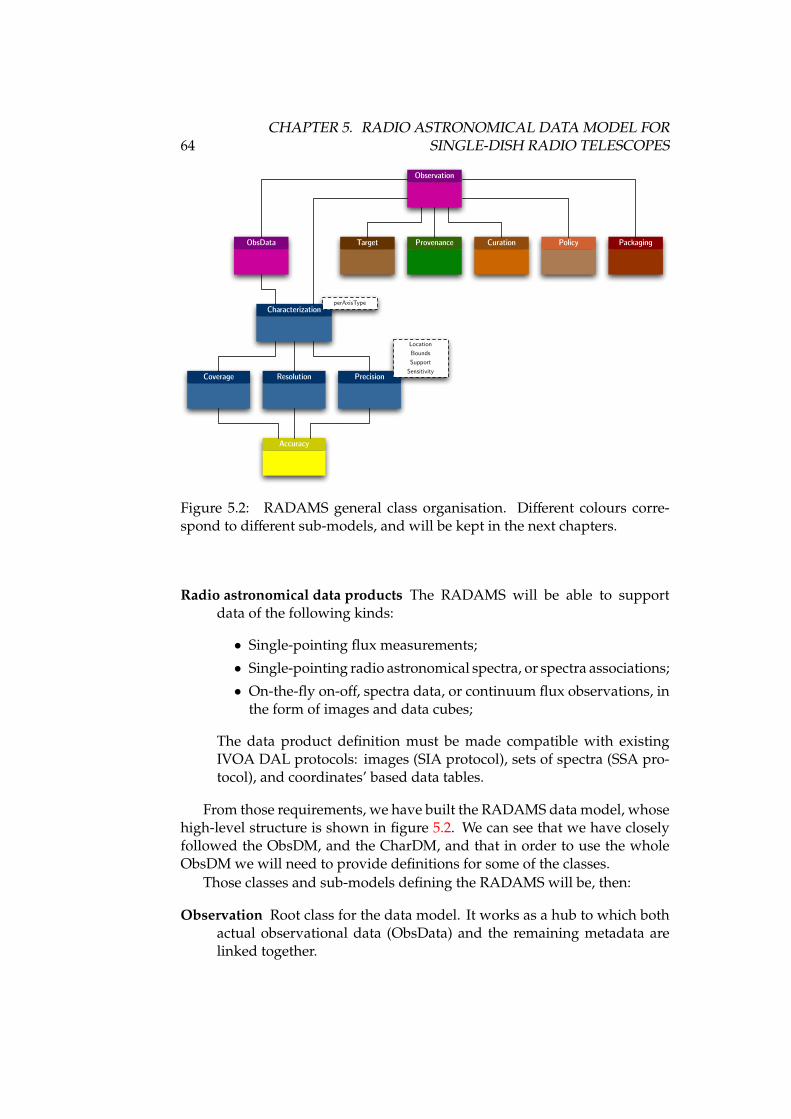
64CHAPTER 5. RADIO ASTRONOMICAL DATA MODEL FOR
SINGLE-DISH RADIO TELESCOPES
Observation
ObsData
Characterization
Coverage Resolution Precision
Target Provenance Curation Policy Packaging
Accuracy
perAxisType
LocationBoundsSupportSensitivity
Figure 5.2: RADAMS general class organisation. Different colours corre-spond to different sub-models, and will be kept in the next chapters.
Radio astronomical data products The RADAMS will be able to supportdata of the following kinds:
• Single-pointing flux measurements;
• Single-pointing radio astronomical spectra, or spectra associations;
• On-the-fly on-off, spectra data, or continuum flux observations, inthe form of images and data cubes;
The data product definition must be made compatible with existingIVOA DAL protocols: images (SIA protocol), sets of spectra (SSA pro-tocol), and coordinates’ based data tables.
From those requirements, we have built the RADAMS data model, whosehigh-level structure is shown in figure 5.2. We can see that we have closelyfollowed the ObsDM, and the CharDM, and that in order to use the wholeObsDM we will need to provide definitions for some of the classes.
Those classes and sub-models defining the RADAMS will be, then:
Observation Root class for the data model. It works as a hub to which bothactual observational data (ObsData) and the remaining metadata arelinked together.
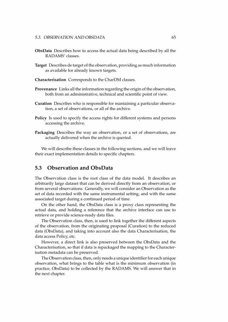
5.3. OBSERVATION AND OBSDATA 65
ObsData Describes how to access the actual data being described by all theRADAMS’ classes.
Target Describes de target of the observation, providing as much informationas available for already known targets.
Characterisation Corresponds to the CharDM classes.
Provenance Links all the information regarding the origin of the observation,both from an administrative, technical and scientific point of view.
Curation Describes who is responsible for mantaining a particular observa-tion, a set of observations, or all of the archive.
Policy Is used to specify the access rights for different systems and personsaccessing the archive.
Packaging Describes the way an observation, or a set of observations, areactually delivered when the archive is queried.
We will describe these classes in the following sections, and we will leavetheir exact implementation details to specific chapters.
5.3 Observation and ObsData
The Observation class is the root class of the data model. It describes anarbitrarily large dataset that can be derived directly from an observation, orfrom several observations. Generally, we will consider an Observation as theset of data recorded with the same instrumental setting, and with the sameassociated target during a continued period of time.
On the other hand, the ObsData class is a proxy class representing theactual data, and holding a reference that the archive interface can use toretrieve or provide science-ready data files.
The Observation class, then, is used to link together the different aspectsof the observation, from the originating proposal (Curation) to the reduceddata (ObsData), and taking into account also the data Characterisation, thedata access Policy, etc.
However, a direct link is also preserved between the ObsData and theCharacterisation, so that if data is repackaged the mapping to the Character-isation metadata can be preserved.
The Observation class, then, only needs a unique identifier for each uniqueobservation, what brings to the table what is the minimum observation (inpractice, ObsData) to be collected by the RADAMS. We will answer that inthe next chapter.
66CHAPTER 5. RADIO ASTRONOMICAL DATA MODEL FOR
SINGLE-DISH RADIO TELESCOPES
5.4 Characterisation
The Characterisation class provides the quantitative and qualitative descrip-tion of the observational data in multiple axes. This information is storedconforming to the most current CharDM IVOA Recommendation [57].
As seen in the previous chapter, we can consider that any astronomicalmeasurement occupies a position in a multi-dimensional space, defined byseveral axes. Initially, this axes are just four (but more can be added): spa-tial (coordinates), temporal, spectral, and a fourth axis corresponding to theobserved physical quantity (e.g., measured flux, or polarisation, in the caseof radio observations). Characterisation gives us a description of the data indifferent attributes and levels of detail inside this multi-dimensional space,including physical units and scales.
The Characterisation class for each individual axis can be divided in thefollowing subclasses:
Coverage Specifies which part of the multi-dimensional space has been en-compassed by the measurement. That is, when was the observationmade and for how long, which field was covered, which bands werestudied, what was the range of observed flux, and so on. Each of thosequestions belongs to a different axis.
Resolution Specifies data resolution in each of the axes. Resolution is inde-pendent of the sampling, as it is a property of the instrument/observingprocess.
Precision If the data are sampled in any axis (e.g., for spectral data in thefrequency domain, data are sampled by means of filter banks, or byFFT from an autocorrelation signal), this class will include informationon the sampling precision. This is different from resolution: resolutionis a property of the instrument, due to uncertainties on the energydistribution of the source, because of convolution of the source’s andthe instrument’s profiles.
Accuracy Specifies the minimum error rate achievable for each axis, bothfrom systematic and random errors.
From this group we can see that for Coverage, Resolution and Precisioninformation can be defined a priori for a whole observing program (in theCharacterisation of a Registry entry, for instance), but they can be differentfor each actual observation dataset, and those will be the ones stored by theRADAMS.
In contrast, Accuracy information needs to be evaluated a posteriori: thelower bounds of accuracy can be known from instrument calibration andknowledge of the observation process, but for some axes assessing the accu-racy actually achieved needs access to historical information.

5.5. TARGET/FIELD 67
5.5 Target/Field
As we have mentioned several times, astronomers study most of the timeobjects they already know, while other times they probe a certain part of thesky to see if there is something new, or even survey a whole region in orderto later exhaustively study that region and all objects they can find in it.
This class allows the RADAMS to include information about observedtargets. Such target can be mapped to known astronomical objects, to detectedsources, to a given field, et cetera. Having this entity in a separate class fromthe Observation one allows to perform queries by Target, and the ability tolink external target information using VO services (such as Sesame, Aladin,the SkyNode interface, et cetera).
In order to be linked with ObsData and Observation classes, the uniqueidentifier for the observation is stored, which allows for queries on giventargets to return observations, but also for observation sets to retrieve Targetinformation.
5.6 Provenance
This class groups all the information describing the way an astronomicaldataset was originated. It has to include the instrumental setting for that par-ticular observation, coordinates for the telescope, weather and atmosphericconditions, and all the information about data pre- and post-processing, whensuch data were created by processing already existing datasets3.
Again, the link with ObsData is the unique observation identifier, but forsome of the information, which are recorded automatically by the engineeringdata collection systems, time-stamps will need to be used to bound the rele-vant information (for instance, focus and pointing calibration observations).
5.7 Policy
In astronomy, observation data are the property of the investigator havingsuggested and planned the observation, for a period which in some casesdepends completely on the observer, which might decide never to release tothe public the observations he made, and in other cases depend on policiesimplemented by the organisation providing the observing facility. Typicalcases are 12 to 24 months of proprietary data from the moment the observationwas performed to the moment the observation is made available to the generalcommunity.
Some observatories have policies where different access rights are avail-able depending on the country or the organisation a particular investigator
3This is already the case for reduced data, which makes extensive use of calibrationinformation, background models and measurements, et cetera.
68CHAPTER 5. RADIO ASTRONOMICAL DATA MODEL FOR
SINGLE-DISH RADIO TELESCOPES
belongs to, due to different agreements between the hosting organisation anddata requesting parties.
This class allows both for the tagging of the observation data, and forestablishing the data access rights for datasets depending on the Policy infor-mation for the dataset itself, and for the user.
Examples of widely different data access policies can be found in archivessuch as the European Southern Observatory Archive4 (ESO). A more generalview on scientific data access policies can be found on the Committee onData for Science and Technology (CODATA) of the International Council forScience (ICSU) on their Scientific Data Policy Statements website5.
In order to accommodate all these different kinds of data access policies,we have chosen a role-based approach, where different permissions are al-lowed not to each different user, but regarding the role that user has againsta particular piece of information. This mechanism will be discussed in detailin chapter 7.2.
5.8 Curation
To be considered part of the VO community, all VO resources have to beincluded in a Registry. The Curation class encompasses all the metadataneeded for well-formed archive and data VO registry. In addition, we alsointegrate an ObservingProgram subclass, proposed by Anita Richards in theDMO document, which acts as an intermediate class that allows groupingtogether different observations with a common goal, such as a any kind ofsurvey, or follow-up observing program, for instance.
Curation information is generated first for the whole archive, and lateron different observations can be associated (via a Packaging different fromthe default for the archive) with a different curator, so that they can either beproperly registered as a different resource, or at least downloaded, packageddata, can refer to the curator for that particular collection.
5.9 Packaging
Archive queries result in different datasets, and a particular dataset for a givenObservation can contain several measurements. The Packaging class specifieswhat is being delivered by the archive as a result for a given query, and theorganisation of data packages different VOTables link to. We will provide an
4The archive of the ESO, for instance, makes header information (including pointing)available immediately after observation, together with calibration data. Actual science dataare only released after a proprietary period (which can be extended under demand), togetherwith observation proposal abstracts. Their policy can be found at http://archive.eso.org/cms/eso-data-access-policy
5http://www.codata.org/data_access/policies.html
5.10. CONCLUSIONS 69
initial development of this class, suitable for the needs of the RADAMS. Wewill also propose a VO general packaging system, the VOPack.
The principles for the VOPack are providing an off-line mechanism for as-sessing the main properties applicable to the whole package of datasets: com-plete Characterisation of Coverage, Resolution, and Precision in all relevantaxes, together with common Curation, Policy, Targets and Data Provenance.
5.10 Conclusions
In this chapter we have shown that a complete version of the ObsDM can beused as a blueprint for building astronomical archives, making easier the taskof building VO services publishing the archive assets.
In a high-level overview, the needs for radio astronomy are quite similarto the needs of astronomy in general: data need to be accessed by coordinates,targets and then spectral and temporal filters applied. We have also shownthat the differences for radio astronomical observations lie in the Charac-terisation part, specially in Spectral coverage, and also in spatial resolution;and in the Provenance class, which deals with the details on how was theobservation observed.
With those specifics in mind, we have built the RADAMS, a Radio Astro-nomical DAta Model for Single-dish observations, which will be used both asa valid blueprint for building a radio astronomical archive from scratch, byvirtue of its implementation of the ObsDM and the CharDM, and the specifi-cation of yet to be defined by the IVOA data models within the ObsDM.
In particular, the data models receiving the most attention from theRADAMS are:
Characterisation Need to characterise radio astronomical observations fromtheir particular properties.
Provenance The origin of the observation in radio astronomy is fundamen-tally different from that of optical observations, as the optical path6 anddetectors are completely different in nature.
Packaging This model, in principle, has no radio astronomical specifics, butit has been developed as a way to provide different kinds of associatedobservations together. In a sense, is a complement to the SpecDM (andthe ObsDM) lack of a way to declare that several observations are notto be independently considered, but that instead form a coherent unitfor scientific analysis.
6Even for non-optical (or non-visible) electromagnetic radiation the path followed byphotons inside a photon collection instrument is called the optical path. The means formaking photons of different wavelengths follow a particular optical path is, as it can beimagined, dependent of the wavelength range.
70CHAPTER 5. RADIO ASTRONOMICAL DATA MODEL FOR
SINGLE-DISH RADIO TELESCOPES
Target Again, this model should not be, in principle, specific to radio astron-omy. It has been defined in a way as general as possible as to be usedfor the SpecDM, the ObsDM, and also be able to host information fromservices such as Simbad, VizieR, and NED, dealing with compilationsof information for named/catalogued sources.
As a result, we will provide specific guidance for the serialisation ofradio astronomical observations in the next chapter, while we will provideadditional details on the Curation, Packaging and Policy data models onchapter 7, leaving the subject of data provenance to chapters 8 and 9.
Chapter 6
RADAMS: Characterising radioastronomical observations
In the previous chapter we analysed how an astronomical archive could bebuilt using the basis of the ObsDM, if the missing data models suggested bythe ObsDM document were to be implemented. We also illustrated how VOcompatibility could be added to archives built on such a basis much moreeasily.
After that, we showed the high level overview of the RADAMS, which wasat first glance almost indistinguishable from the ObsDM, something which isindeed a feature of the RADAMS. Finally, we provided a first overview of thedefinition of each particular class and sub-models, and the way they meshtogether.
Once we have introduced the RADAMS, we will start studying it in detailin this and the following chapters. In particular, this chapter will be devotedto how the RADAMS stores the Observation and ObsData information, andhow the CharDM data model is filled for the different observation modes inradio telescopes.
In addition, in those chapters devoted to the detailed exploration of theRADAMS, we will select appropriate FITS Keywords and UCDs for FITSand VOTable serialisations of observational data. FITS Keywords will beselected first from the official FITS mandatory headers [65]. If no mandatorykeyword exists, they will be chosen from the Multi-Beam FITS Raw DataFormat [22], and lastly from the NRAO GBT FITS data format [66]1. Whereassign appears, it means that a suitable FITS keyword has yet to be selectedfor that particular database attribute.
UCDs will be selected from the UCD1+ vocabulary [67], using the rec-ommended juxtaposition technique in order to clarify the meaning of anygiven term. In some cases, there are no existing UCD atoms, and no UCD
1Sometimes those keywords cannot appear in the main header of a FITS file, but insteadin a FITS extension table, but that will not be specified.
71
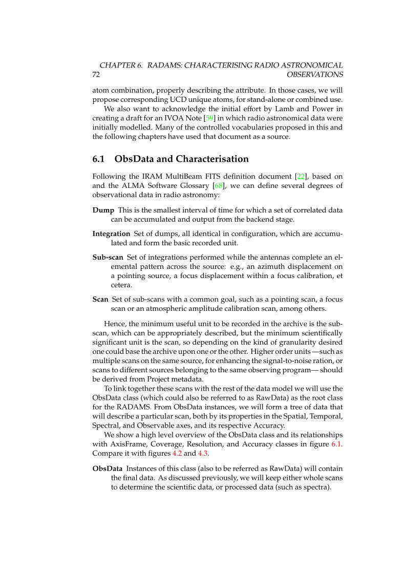
72CHAPTER 6. RADAMS: CHARACTERISING RADIO ASTRONOMICAL
OBSERVATIONS
atom combination, properly describing the attribute. In those cases, we willpropose corresponding UCD unique atoms, for stand-alone or combined use.
We also want to acknowledge the initial effort by Lamb and Power increating a draft for an IVOA Note [59] in which radio astronomical data wereinitially modelled. Many of the controlled vocabularies proposed in this andthe following chapters have used that document as a source.
6.1 ObsData and Characterisation
Following the IRAM MultiBeam FITS definition document [22], based onand the ALMA Software Glossary [68], we can define several degrees ofobservational data in radio astronomy:
Dump This is the smallest interval of time for which a set of correlated datacan be accumulated and output from the backend stage.
Integration Set of dumps, all identical in configuration, which are accumu-lated and form the basic recorded unit.
Sub-scan Set of integrations performed while the antennas complete an el-emental pattern across the source: e.g., an azimuth displacement ona pointing source, a focus displacement within a focus calibration, etcetera.
Scan Set of sub-scans with a common goal, such as a pointing scan, a focusscan or an atmospheric amplitude calibration scan, among others.
Hence, the minimum useful unit to be recorded in the archive is the sub-scan, which can be appropriately described, but the minimum scientificallysignificant unit is the scan, so depending on the kind of granularity desiredone could base the archive upon one or the other. Higher order units —such asmultiple scans on the same source, for enhancing the signal-to-noise ration, orscans to different sources belonging to the same observing program— shouldbe derived from Project metadata.
To link together these scans with the rest of the data model we will use theObsData class (which could also be referred to as RawData) as the root classfor the RADAMS. From ObsData instances, we will form a tree of data thatwill describe a particular scan, both by its properties in the Spatial, Temporal,Spectral, and Observable axes, and its respective Accuracy.
We show a high level overview of the ObsData class and its relationshipswith AxisFrame, Coverage, Resolution, and Accuracy classes in figure 6.1.Compare it with figures 4.2 and 4.3.
ObsData Instances of this class (also to be referred as RawData) will containthe final data. As discussed previously, we will keep either whole scansto determine the scientific data, or processed data (such as spectra).
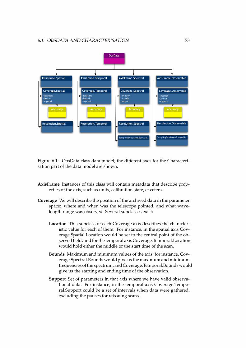
6.1. OBSDATA AND CHARACTERISATION 73
ObsData
AxisFrame.Observable
-location-bounds-support
Coverage.Observable
Accuracy
Resolution.Observable
SamplingPrecision.Observable
AxisFrame.Spectral
Accuracy
-location-bounds-support
Coverage.Spectral
Resolution.Spectral
SamplingPrecision.Spectral
AxisFrame.Temporal
-location-bounds-support
Coverage.Temporal
Accuracy
Resolution.Temporal
AxisFrame.Spatial
-location-bounds-support
Coverage.Spatial
Accuracy
Resolution.Spatial
Figure 6.1: ObsData class data model; the different axes for the Characteri-sation part of the data model are shown.
AxisFrame Instances of this class will contain metadata that describe prop-erties of the axis, such as units, calibration state, et cetera.
Coverage We will describe the position of the archived data in the parameterspace: where and when was the telescope pointed, and what wave-length range was observed. Several subclasses exist:
Location This subclass of each Coverage axis describes the character-istic value for each of them. For instance, in the spatial axis Cov-erage.Spatial.Location would be set to the central point of the ob-served field, and for the temporal axis Coverage.Temporal.Locationwould hold either the middle or the start time of the scan.
Bounds Maximum and minimum values of the axis; for instance, Cov-erage.Spectral.Bounds would give us the maximum and minimumfrequencies of the spectrum, and Coverage.Temporal.Bounds wouldgive us the starting and ending time of the observation.
Support Set of parameters in that axis where we have valid observa-tional data. For instance, in the temporal axis Coverage.Tempo-ral.Support could be a set of intervals when data were gathered,excluding the pauses for reissuing scans.
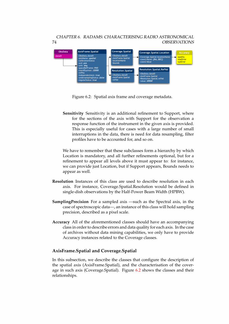
74CHAPTER 6. RADAMS: CHARACTERISING RADIO ASTRONOMICAL
OBSERVATIONS
-dataID
ObsData
+ObsData.dataID-axisName: spatial-calibrationStatus-ucd: pos-unit: deg-spaceRefFrame: FK5-coordEquinox: J2000-refPos-independentAxis: true-undersamplingStatus: false-regularStatus: true
AxisFrame.Spatial
+ObsData.dataID+AxisFrame.Spatial-refVal
Resolution.Spatial
+ObsData.dataID+AxisFrame.Spatial-locationName-bounds
Coverage.Spatial
-quality-statError-sysError
Accuracy
+ObsData.dataID+AxisFrame.Spatial+Resolution.Spatial.refVal-value: HPBW
Resolution.Spatial.RefVal
+Coverage.Spatial.locationName-coord.Name: RA, DEC-coord.Value
Coverage.Spatial.Location
Figure 6.2: Spatial axis frame and coverage metadata.
Sensitivity Sensitivity is an additional refinement to Support, wherefor the sections of the axis with Support for the observation aresponse function of the instrument in the given axis is provided.This is especially useful for cases with a large number of smallinterruptions in the data, there is need for data resampling, filterprofiles have to be accounted for, and so on.
We have to remember that these subclasses form a hierarchy by whichLocation is mandatory, and all further refinements optional, but for arefinement to appear all levels above it must appear to: for instance,we can provide just Location, but if Support appears, Bounds needs toappear as well.
Resolution Instances of this class are used to describe resolution in eachaxis. For instance, Coverage.Spatial.Resolution would be defined insingle-dish observations by the Half-Power Beam Width (HPBW).
SamplingPrecision For a sampled axis —such as the Spectral axis, in thecase of spectroscopic data—, an instance of this class will hold samplingprecision, described as a pixel scale.
Accuracy All of the aforementioned classes should have an accompanyingclass in order to describe errors and data quality for each axis. In the caseof archives without data mining capabilities, we only have to provideAccuracy instances related to the Coverage classes.
AxisFrame.Spatial and Coverage.Spatial
In this subsection, we describe the classes that configure the description ofthe spatial axis (AxisFrame.Spatial), and the characterisation of the cover-age in such axis (Coverage.Spatial). Figure 6.2 shows the classes and theirrelationships.
6.1. OBSDATA AND CHARACTERISATION 75
AxisFrame.Spatial This instance describes the properties of the Spatial axis,such as calibration status, units (normally, degrees), reference frame,epoch, spatial sampling type and sampling status, et cetera.
For the DSS-63 antenna, the spatial axis is never sampled (because weare not storing maps at this stage), and each scan only needs two pairs ofcoordinates (plus pointing accuracy) to describe the antenna-pointingpattern.
As the coordinate space is in this case bi-dimensional, and properties forone of the coordinates do not have to be equal for the other, we shouldeither choose between a vector approach, using two dimensional arraysof coordinates, or splitting the Spatial classes in different subclasses. Wechoose the first approach, and thus all AxisFrame.Spatial attributes willhave a space-separated array of values (just two values separated withan space, for a bi-dimensional coordinate space).
If the archive were to be exploited in the third dimension, an additionaldistance and/or redshift coordinate should be entered. As we have seen,extension in the spatial axis is straightforward. A second option wouldadd an additional axis to the Characterisation data model.
Coverage.Spatial.Location For the DSS-63 antenna, the stored values forthis class correspond to the antenna pointing coordinates. If a Targetis linked, Spatial.Location information sould be the same, unless thetarget is not directly associated, but found by cross-correlation with theTargets database.
Coverage.Spatial.Bounds Bounds for spatial data would be the maximumand minimum for spatial coordinates (normally, right ascension anddeclination) when observing the source. For single point spectroscopicdata, this class is not needed, as the antenna does not describe any pathacross the source.
Coverage.Spatial.Support Typically, the stored values for this class shouldbe equal to those of Coverage.Spatial.Bounds, except when invalid datawithin Coverage.Spatial.Bounds might exist, or in order to describe anelaborate scanning path on the source. This class would describe sucha path.
Coverage.Spatial.Sensitivity In the case of the DSS-63 antenna, Spatial.Sen-sitivity would be defined as the beam pattern of the antenna, in principlein 1D taking symmetries into account, but 2D could be considered, asit would be the case for a synthesised beam in interferometry. Anotherpossibility is the combination of beam pattern with receiver efficiencyat different elevations.
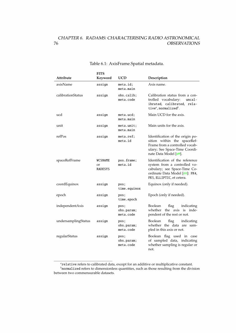
76CHAPTER 6. RADAMS: CHARACTERISING RADIO ASTRONOMICAL
OBSERVATIONS
Table 6.1: AxisFrame.Spatial metadata.
FITSAttribute Keyword UCD Description
axisName assign meta.id;meta.main
Axis name.
calibrationStatus assign obs.calib;meta.code
Calibration status from a con-trolled vocabulary: uncal-ibrated, calibrated, rela-tivea, normalizedb.
ucd assign meta.ucd;meta.main
Main UCD for the axis.
unit assign meta.unit;meta.main
Main units for the axis.
refPos assign meta.ref;meta.id
Identification of the origin po-sition within the spaceRef-Frame from a controlled vocab-ulary; See Space-Time Coordi-nate Data Model [69].
spaceRefFrame WCSNAMEorRADESYS
pos.frame;meta.id
Identification of the referencesystem from a controlled vo-cabulary; see Space-Time Co-ordinate Data Model [69]: FK4,FK5, ELLIPTIC, et cetera.
coordEquinox assign pos;time.equinox
Equinox (only if needed).
epoch assign pos;time.epoch
Epoch (only if needed).
independentAxis assign pos;obs.param;meta.code
Boolean flag indicatingwhether the axis is inde-pendent of the rest or not.
undersamplingStatus assign pos;obs.param;meta.code
Boolean flag indicatingwhether the data are sam-pled in this axis or not.
regularStatus assign pos;obs.param;meta.code
Boolean flag used in caseof sampled data, indicatingwhether sampling is regular ornot.
arelative refers to calibrated data, except for an additive or multiplicative constant.bnormalized refers to dimensionless quantities, such as those resulting from the division
between two commensurable datasets.
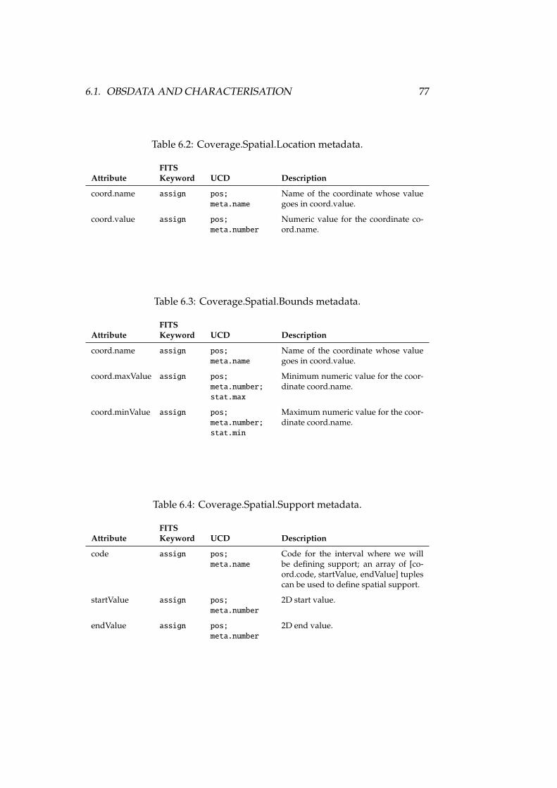
6.1. OBSDATA AND CHARACTERISATION 77
Table 6.2: Coverage.Spatial.Location metadata.
FITSAttribute Keyword UCD Description
coord.name assign pos;meta.name
Name of the coordinate whose valuegoes in coord.value.
coord.value assign pos;meta.number
Numeric value for the coordinate co-ord.name.
Table 6.3: Coverage.Spatial.Bounds metadata.
FITSAttribute Keyword UCD Description
coord.name assign pos;meta.name
Name of the coordinate whose valuegoes in coord.value.
coord.maxValue assign pos;meta.number;stat.max
Minimum numeric value for the coor-dinate coord.name.
coord.minValue assign pos;meta.number;stat.min
Maximum numeric value for the coor-dinate coord.name.
Table 6.4: Coverage.Spatial.Support metadata.
FITSAttribute Keyword UCD Description
code assign pos;meta.name
Code for the interval where we willbe defining support; an array of [co-ord.code, startValue, endValue] tuplescan be used to define spatial support.
startValue assign pos;meta.number
2D start value.
endValue assign pos;meta.number
2D end value.
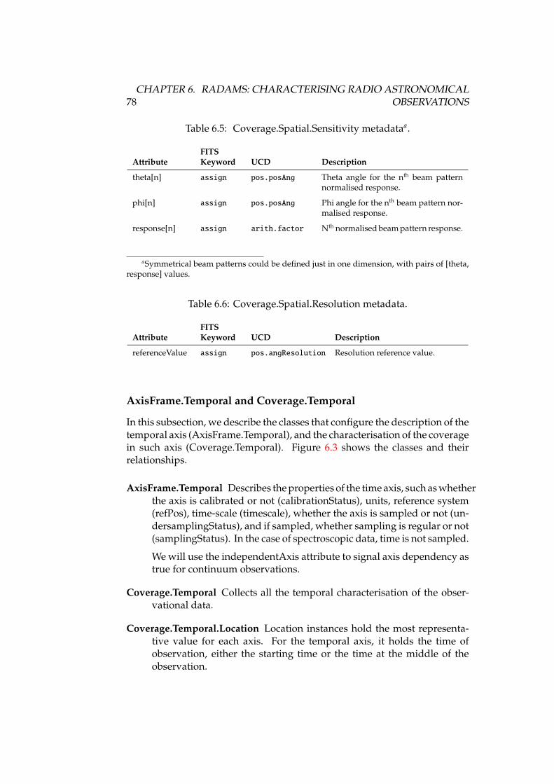
78CHAPTER 6. RADAMS: CHARACTERISING RADIO ASTRONOMICAL
OBSERVATIONS
Table 6.5: Coverage.Spatial.Sensitivity metadataa.
FITSAttribute Keyword UCD Description
theta[n] assign pos.posAng Theta angle for the nth beam patternnormalised response.
phi[n] assign pos.posAng Phi angle for the nth beam pattern nor-malised response.
response[n] assign arith.factor Nth normalised beam pattern response.
aSymmetrical beam patterns could be defined just in one dimension, with pairs of [theta,response] values.
Table 6.6: Coverage.Spatial.Resolution metadata.
FITSAttribute Keyword UCD Description
referenceValue assign pos.angResolution Resolution reference value.
AxisFrame.Temporal and Coverage.Temporal
In this subsection, we describe the classes that configure the description of thetemporal axis (AxisFrame.Temporal), and the characterisation of the coveragein such axis (Coverage.Temporal). Figure 6.3 shows the classes and theirrelationships.
AxisFrame.Temporal Describes the properties of the time axis, such as whetherthe axis is calibrated or not (calibrationStatus), units, reference system(refPos), time-scale (timescale), whether the axis is sampled or not (un-dersamplingStatus), and if sampled, whether sampling is regular or not(samplingStatus). In the case of spectroscopic data, time is not sampled.
We will use the independentAxis attribute to signal axis dependency astrue for continuum observations.
Coverage.Temporal Collects all the temporal characterisation of the obser-vational data.
Coverage.Temporal.Location Location instances hold the most representa-tive value for each axis. For the temporal axis, it holds the time ofobservation, either the starting time or the time at the middle of theobservation.
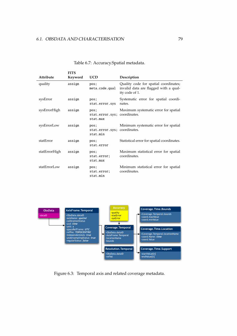
6.1. OBSDATA AND CHARACTERISATION 79
Table 6.7: Accuracy.Spatial metadata.
FITSAttribute Keyword UCD Description
quality assign pos;meta.code.qual
Quality code for spatial coordinates;invalid data are flagged with a qual-ity code of 1.
sysError assign pos;stat.error.sys
Systematic error for spatial coordi-nates.
sysErrorHigh assign pos;stat.error.sys;stat.max
Maximum systematic error for spatialcoordinates.
sysErrorLow assign pos;stat.error.sys;stat.min
Minimum systematic error for spatialcoordinates.
statError assign pos;stat.error
Statistical error for spatial coordinates.
statErrorHigh assign pos;stat.error;stat.max
Maximum statistical error for spatialcoordinates.
statErrorLow assign pos;stat.error;stat.min
Minimum statistical error for spatialcoordinates.
-dataID
ObsData
+ObsData.dataID-axisName: spatial-calibrationStatus-ucd: time-unit: s-spaceRefFrame: UTC-refPos: TOPOCENTRIC-independentAxis: true-undersamplingStatus: true-regularStatus: false
AxisFrame.Temporal
+ObsData.dataID-refVal
Resolution.Temporal
+ObsData.dataID+AxisFrame.Temporal-locationName-bounds
Coverage.Temporal
-quality-statError-sysError
Accuracy
+Coverage.Temporal.locationName-coord.Name: time-coord.Value
Coverage.Time.Location
+Coverage.Temporal.bounds-coord.maxValue-coord.minValue
Coverage.Time.Bounds
-startValue[n]-endValue[n]
Coverage.Time.Support
Figure 6.3: Temporal axis and related coverage metadata.
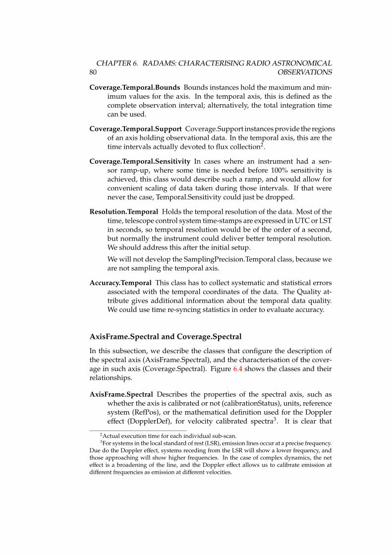
80CHAPTER 6. RADAMS: CHARACTERISING RADIO ASTRONOMICAL
OBSERVATIONS
Coverage.Temporal.Bounds Bounds instances hold the maximum and min-imum values for the axis. In the temporal axis, this is defined as thecomplete observation interval; alternatively, the total integration timecan be used.
Coverage.Temporal.Support Coverage.Support instances provide the regionsof an axis holding observational data. In the temporal axis, this are thetime intervals actually devoted to flux collection2.
Coverage.Temporal.Sensitivity In cases where an instrument had a sen-sor ramp-up, where some time is needed before 100% sensitivity isachieved, this class would describe such a ramp, and would allow forconvenient scaling of data taken during those intervals. If that werenever the case, Temporal.Sensitivity could just be dropped.
Resolution.Temporal Holds the temporal resolution of the data. Most of thetime, telescope control system time-stamps are expressed in UTC or LSTin seconds, so temporal resolution would be of the order of a second,but normally the instrument could deliver better temporal resolution.We should address this after the initial setup.
We will not develop the SamplingPrecision.Temporal class, because weare not sampling the temporal axis.
Accuracy.Temporal This class has to collect systematic and statistical errorsassociated with the temporal coordinates of the data. The Quality at-tribute gives additional information about the temporal data quality.We could use time re-syncing statistics in order to evaluate accuracy.
AxisFrame.Spectral and Coverage.Spectral
In this subsection, we describe the classes that configure the description ofthe spectral axis (AxisFrame.Spectral), and the characterisation of the cover-age in such axis (Coverage.Spectral). Figure 6.4 shows the classes and theirrelationships.
AxisFrame.Spectral Describes the properties of the spectral axis, such aswhether the axis is calibrated or not (calibrationStatus), units, referencesystem (RefPos), or the mathematical definition used for the Dopplereffect (DopplerDef), for velocity calibrated spectra3. It is clear that
2Actual execution time for each individual sub-scan.3For systems in the local standard of rest (LSR), emission lines occur at a precise frequency.
Due do the Doppler effect, systems receding from the LSR will show a lower frequency, andthose approaching will show higher frequencies. In the case of complex dynamics, the neteffect is a broadening of the line, and the Doppler effect allows us to calibrate emission atdifferent frequencies as emission at different velocities.
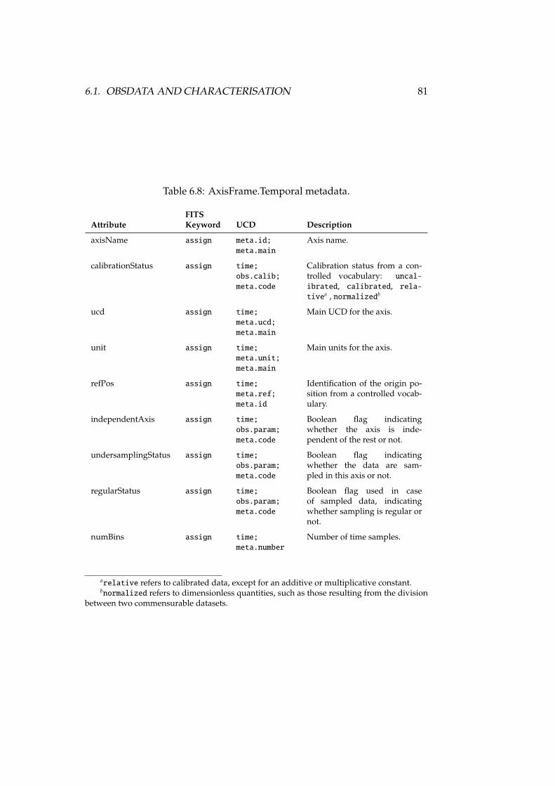
6.1. OBSDATA AND CHARACTERISATION 81
Table 6.8: AxisFrame.Temporal metadata.
FITSAttribute Keyword UCD Description
axisName assign meta.id;meta.main
Axis name.
calibrationStatus assign time;obs.calib;meta.code
Calibration status from a con-trolled vocabulary: uncal-ibrated, calibrated, rela-tivea , normalizedb
ucd assign time;meta.ucd;meta.main
Main UCD for the axis.
unit assign time;meta.unit;meta.main
Main units for the axis.
refPos assign time;meta.ref;meta.id
Identification of the origin po-sition from a controlled vocab-ulary.
independentAxis assign time;obs.param;meta.code
Boolean flag indicatingwhether the axis is inde-pendent of the rest or not.
undersamplingStatus assign time;obs.param;meta.code
Boolean flag indicatingwhether the data are sam-pled in this axis or not.
regularStatus assign time;obs.param;meta.code
Boolean flag used in caseof sampled data, indicatingwhether sampling is regular ornot.
numBins assign time;meta.number
Number of time samples.
arelative refers to calibrated data, except for an additive or multiplicative constant.bnormalized refers to dimensionless quantities, such as those resulting from the division
between two commensurable datasets.
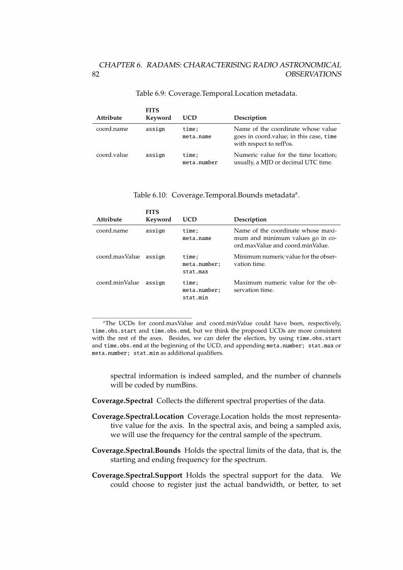
82CHAPTER 6. RADAMS: CHARACTERISING RADIO ASTRONOMICAL
OBSERVATIONS
Table 6.9: Coverage.Temporal.Location metadata.
FITSAttribute Keyword UCD Description
coord.name assign time;meta.name
Name of the coordinate whose valuegoes in coord.value; in this case, timewith respect to refPos.
coord.value assign time;meta.number
Numeric value for the time location;usually, a MJD or decimal UTC time.
Table 6.10: Coverage.Temporal.Bounds metadataa.
FITSAttribute Keyword UCD Description
coord.name assign time;meta.name
Name of the coordinate whose maxi-mum and minimum values go in co-ord.maxValue and coord.minValue.
coord.maxValue assign time;meta.number;stat.max
Minimum numeric value for the obser-vation time.
coord.minValue assign time;meta.number;stat.min
Maximum numeric value for the ob-servation time.
aThe UCDs for coord.maxValue and coord.minValue could have been, respectively,time.obs.start and time.obs.end, but we think the proposed UCDs are more consistentwith the rest of the axes. Besides, we can defer the election, by using time.obs.startand time.obs.end at the beginning of the UCD, and appending meta.number; stat.max ormeta.number; stat.min as additional qualifiers.
spectral information is indeed sampled, and the number of channelswill be coded by numBins.
Coverage.Spectral Collects the different spectral properties of the data.
Coverage.Spectral.Location Coverage.Location holds the most representa-tive value for the axis. In the spectral axis, and being a sampled axis,we will use the frequency for the central sample of the spectrum.
Coverage.Spectral.Bounds Holds the spectral limits of the data, that is, thestarting and ending frequency for the spectrum.
Coverage.Spectral.Support Holds the spectral support for the data. Wecould choose to register just the actual bandwidth, or better, to set

6.1. OBSDATA AND CHARACTERISATION 83
Table 6.11: Coverage.Temporal.Support metadataa.
FITSAttribute Keyword UCD Description
code assign time;meta.code
Code for the time interval where wewill be defining support; an array of[coord.code, startValue, endValue] tu-ples can be used to define temporalsupport.
startValue assign time.expo.start Time interval start value.
endValue assign time.expo.end 2DTime interval end value.
aCoverage.Temporal.Support could be alternatively defined by using just one value, theexposure time, with UCD time.expo. The chosen definition, apart from being more consistentacross axes, allows for discontinuous temporal support.
Table 6.12: Coverage.Temporal.Resolution metadata.
FITSAttribute Keyword UCD Description
referenceValue assign time;meta.number;meta.ref
Resolution reference value.
an array of different intervals where the instrument is sensitive. Betteryet, we could register a sensitivity profile for each frequency. We willinitially choose the array of intervals as the way to express the spectralsupport.
Coverage.Spectral.Sensitivity Holds the sensitivity profile for the instru-ment in frequency; in other words, this would be equal to the detailedfrequency response of the whole antenna-receiver-backend set.
Resolution.Spectral Holds the spectral resolution information for the data.For filter banks, it is the filter bandwidth for each filter, or an aver-age filter bandwidth. In the case of spectra obtained from the Fouriertransform of the autocorrelation function, it is equal to the bandwidthdivided by the number of channels.
SamplingPrecision.Spectral In the case of the Robledo antenna, this valueshould be equal to the value stored at Resolution.Spectral. For other in-struments, SamplingPrecision.Spectral defines the frequency steps fromone frequency bin to the next.
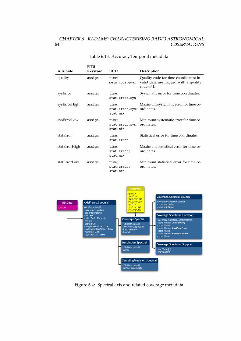
84CHAPTER 6. RADAMS: CHARACTERISING RADIO ASTRONOMICAL
OBSERVATIONS
Table 6.13: Accuracy.Temporal metadata.
FITSAttribute Keyword UCD Description
quality assign time;meta.code.qual
Quality code for time coordinates; in-valid data are flagged with a qualitycode of 1.
sysError assign time;stat.error.sys
Systematic error for time coordinates.
sysErrorHigh assign time;stat.error.sys;stat.max
Maximum systematic error for time co-ordinates.
sysErrorLow assign time;stat.error.sys;stat.min
Minimum systematic error for time co-ordinates.
statError assign time;stat.error
Statistical error for time coordinates.
statErrorHigh assign time;stat.error;stat.max
Maximum statistical error for time co-ordinates.
statErrorLow assign time;stat.error;stat.min
Minimum statistical error for time co-ordinates.
-dataID
ObsData
+ObsData.dataID-axisName: spatial-calibrationStatus-ucd: em-unit: Tmb, Tsky, Jy-refPos:-dopplerDef-independentAxis: true-undersamplingStatus: false-numBins: 384-regularStatus: true
AxisFrame.Spectral
+ObsData.dataID-refVal
Resolution.Spectral
+ObsData.dataID+AxisFrame.Spectral-locationName-bounds
Coverage.Spectral
-quality-statError-statErrorHigh-statErrorLow-sysError-sysErrorHigh-sysErrorLow
Accuracy
+Coverage.Spectral.locationName-coord.Name: CentralFreq-coord.Value-coord.Name: MaxPeakFreq-coord.Value-coord.Name: MaxPeakValue-coord.Value
Coverage.Spectrum.Location
+Coverage.Spectral.bounds-coord.maxValue-coord.minValue
Coverage.Spectral.Bounds
-startValue[n]-endValue[n]
Coverage.Spectrum.Support
+ObsData.dataID-refVal: pixelScale
SamplingPrecision.Spectral
Figure 6.4: Spectral axis and related coverage metadata.

6.1. OBSDATA AND CHARACTERISATION 85
Accuracy.Spectral Errors associated with the spectrum. In the same way asthe support could change along the spectrum, because of different sensi-tivities, we might need to characterise the accuracy along the spectrum.At least in the case of Robledo, the SNR is global, and considered equalfor all frequencies. If not, a first approximation can be using an averageSNR, and maximum and minimum SNR.
AxisFrame.Observable and Coverage.Observable
The Observable axis is, finally, the one directly related to the stored data, in-stead of data headers. In this subsection, we describe the classes that configurethe description of the observable axis (AxisFrame.Observable), and the char-acterisation of the coverage in such axis (Coverage.Observable). Figure 6.5shows the classes and their relationships.
AxisFrame.Observable Describes the properties of the observable axis (whetherthe observable is flux, polarisation state, or any other), such as whetherthe data is calibrated or not (calibrationStatus), applicable units, etcetera. Flux information is sampled at the digital conversion stage,and the number of available different flux levels is codified in numBins.By specifying units in this class, we define whether the observable dataare provided in flux units, or in brightness or antenna temperature. Ad-ditional information, such as the polarisation, can be accommodated inthe same axis in the same way we extended the Spatial axis for 2D or3D coordinates, or by means of (an) additional observable (axis) axes.
Coverage.Observable Collects all information that directly characterises ob-servable data.
Coverage.Observable.Location Coverage.Location instances hold the mostrepresentative value for that axis. In this case, the average spectrum fluxis not significant, specially if we have a strong line detection. Hence,for this axis we will take the maximum flux as Observable.Location.
Coverage.Observable.Bounds Coverage.Bounds instances record the max-imum and minimum values for the axis. In the Observable axis, itrecords minimum and maximum flux for the spectrum.
Coverage.Observable.Support This instance should give us the intervals offlux observed in the spectrum, and we could choose between mak-ing it equal to Coverage.Observable.Bounds, or defining an intervalthat holds a given dispersion from the Coverage.Observable.Locationvalue. We will initially consider Coverage.Observable.Support as equalto Coverage.Observable.Bounds.
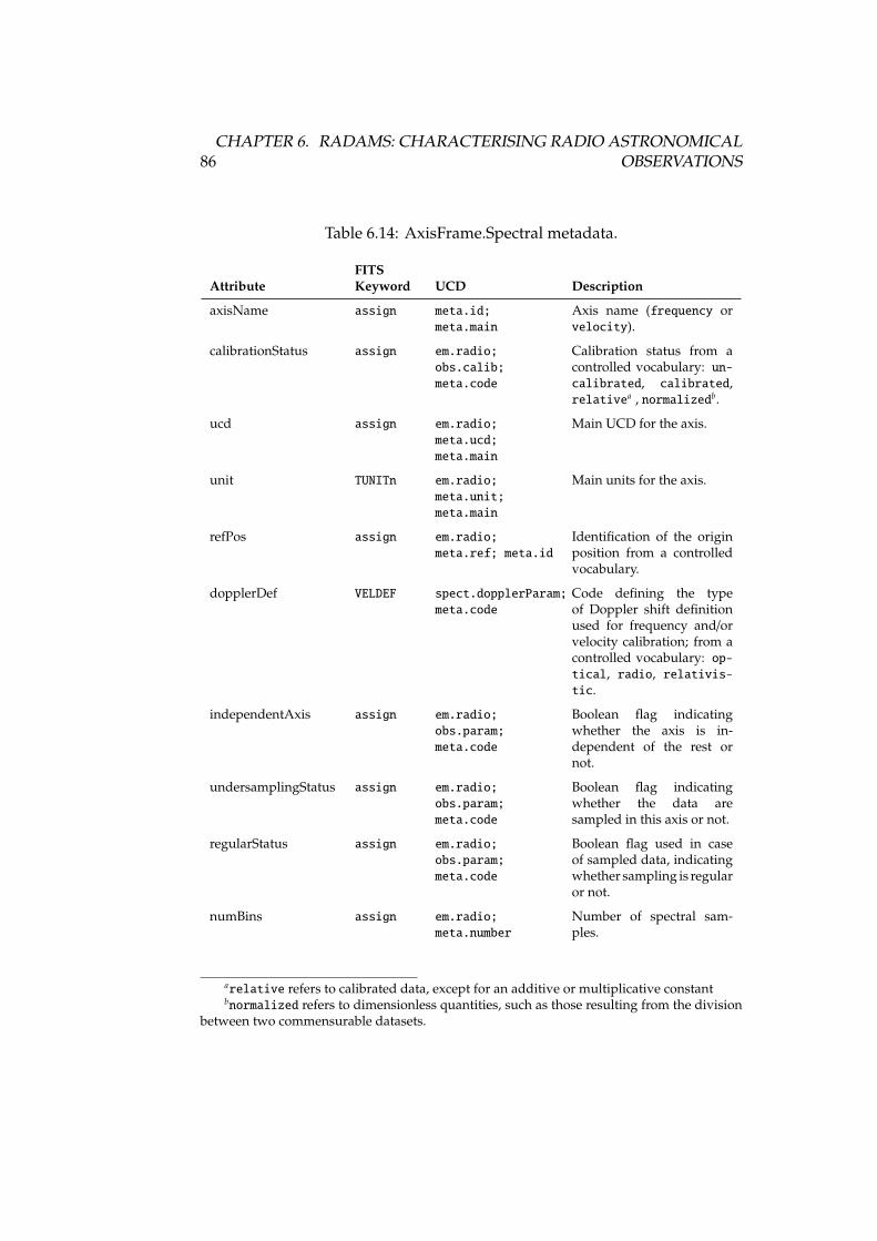
86CHAPTER 6. RADAMS: CHARACTERISING RADIO ASTRONOMICAL
OBSERVATIONS
Table 6.14: AxisFrame.Spectral metadata.
FITSAttribute Keyword UCD Description
axisName assign meta.id;meta.main
Axis name (frequency orvelocity).
calibrationStatus assign em.radio;obs.calib;meta.code
Calibration status from acontrolled vocabulary: un-calibrated, calibrated,relativea , normalizedb.
ucd assign em.radio;meta.ucd;meta.main
Main UCD for the axis.
unit TUNITn em.radio;meta.unit;meta.main
Main units for the axis.
refPos assign em.radio;meta.ref; meta.id
Identification of the originposition from a controlledvocabulary.
dopplerDef VELDEF spect.dopplerParam;meta.code
Code defining the typeof Doppler shift definitionused for frequency and/orvelocity calibration; from acontrolled vocabulary: op-tical, radio, relativis-tic.
independentAxis assign em.radio;obs.param;meta.code
Boolean flag indicatingwhether the axis is in-dependent of the rest ornot.
undersamplingStatus assign em.radio;obs.param;meta.code
Boolean flag indicatingwhether the data aresampled in this axis or not.
regularStatus assign em.radio;obs.param;meta.code
Boolean flag used in caseof sampled data, indicatingwhether sampling is regularor not.
numBins assign em.radio;meta.number
Number of spectral sam-ples.
arelative refers to calibrated data, except for an additive or multiplicative constantbnormalized refers to dimensionless quantities, such as those resulting from the division
between two commensurable datasets.
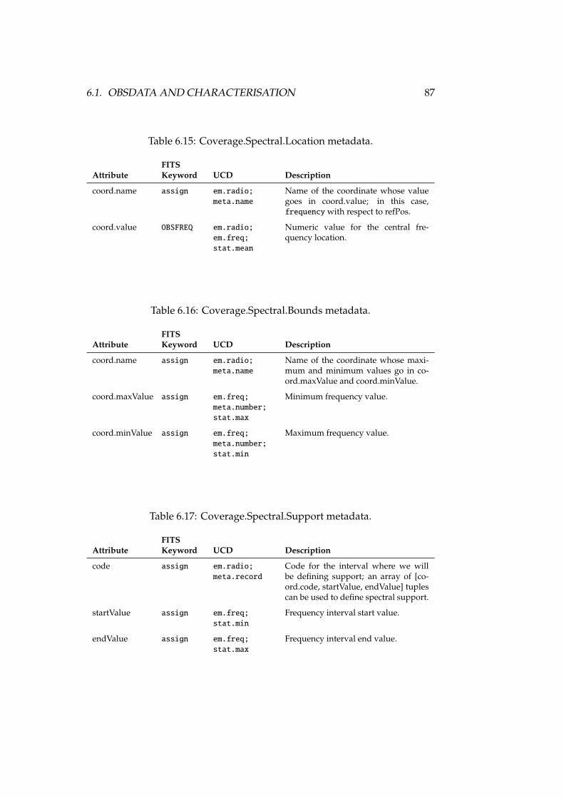
6.1. OBSDATA AND CHARACTERISATION 87
Table 6.15: Coverage.Spectral.Location metadata.
FITSAttribute Keyword UCD Description
coord.name assign em.radio;meta.name
Name of the coordinate whose valuegoes in coord.value; in this case,frequency with respect to refPos.
coord.value OBSFREQ em.radio;em.freq;stat.mean
Numeric value for the central fre-quency location.
Table 6.16: Coverage.Spectral.Bounds metadata.
FITSAttribute Keyword UCD Description
coord.name assign em.radio;meta.name
Name of the coordinate whose maxi-mum and minimum values go in co-ord.maxValue and coord.minValue.
coord.maxValue assign em.freq;meta.number;stat.max
Minimum frequency value.
coord.minValue assign em.freq;meta.number;stat.min
Maximum frequency value.
Table 6.17: Coverage.Spectral.Support metadata.
FITSAttribute Keyword UCD Description
code assign em.radio;meta.record
Code for the interval where we willbe defining support; an array of [co-ord.code, startValue, endValue] tuplescan be used to define spectral support.
startValue assign em.freq;stat.min
Frequency interval start value.
endValue assign em.freq;stat.max
Frequency interval end value.
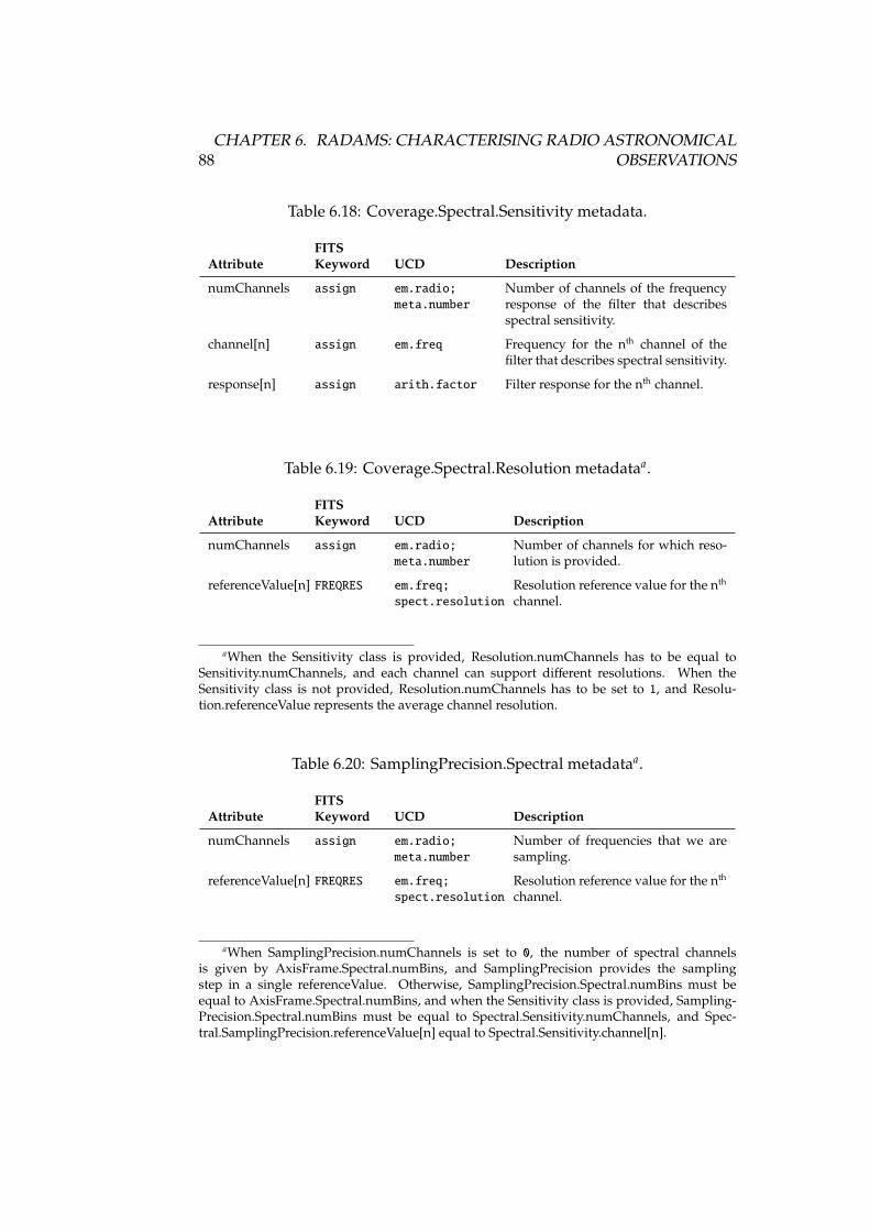
88CHAPTER 6. RADAMS: CHARACTERISING RADIO ASTRONOMICAL
OBSERVATIONS
Table 6.18: Coverage.Spectral.Sensitivity metadata.
FITSAttribute Keyword UCD Description
numChannels assign em.radio;meta.number
Number of channels of the frequencyresponse of the filter that describesspectral sensitivity.
channel[n] assign em.freq Frequency for the nth channel of thefilter that describes spectral sensitivity.
response[n] assign arith.factor Filter response for the nth channel.
Table 6.19: Coverage.Spectral.Resolution metadataa.
FITSAttribute Keyword UCD Description
numChannels assign em.radio;meta.number
Number of channels for which reso-lution is provided.
referenceValue[n] FREQRES em.freq;spect.resolution
Resolution reference value for the nth
channel.
aWhen the Sensitivity class is provided, Resolution.numChannels has to be equal toSensitivity.numChannels, and each channel can support different resolutions. When theSensitivity class is not provided, Resolution.numChannels has to be set to 1, and Resolu-tion.referenceValue represents the average channel resolution.
Table 6.20: SamplingPrecision.Spectral metadataa.
FITSAttribute Keyword UCD Description
numChannels assign em.radio;meta.number
Number of frequencies that we aresampling.
referenceValue[n] FREQRES em.freq;spect.resolution
Resolution reference value for the nth
channel.
aWhen SamplingPrecision.numChannels is set to 0, the number of spectral channelsis given by AxisFrame.Spectral.numBins, and SamplingPrecision provides the samplingstep in a single referenceValue. Otherwise, SamplingPrecision.Spectral.numBins must beequal to AxisFrame.Spectral.numBins, and when the Sensitivity class is provided, Sampling-Precision.Spectral.numBins must be equal to Spectral.Sensitivity.numChannels, and Spec-tral.SamplingPrecision.referenceValue[n] equal to Spectral.Sensitivity.channel[n].
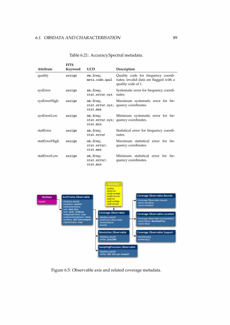
6.1. OBSDATA AND CHARACTERISATION 89
Table 6.21: Accuracy.Spectral metadata.
FITSAttribute Keyword UCD Description
quality assign em.freq;meta.code.qual
Quality code for frequency coordi-nates; invalid data are flagged with aquality code of 1.
sysError assign em.freq;stat.error.sys
Systematic error for frequency coordi-nates.
sysErrorHigh assign em.freq;stat.error.sys;stat.max
Maximum systematic error for fre-quency coordinates.
sysErrorLow assign em.freq;stat.error.sys;stat.min
Minimum systematic error for fre-quency coordinates.
statError assign em.freq;stat.error
Statistical error for frequency coordi-nates.
statErrorHigh assign em.freq;stat.error;stat.max
Maximum statistical error for fre-quency coordinates.
statErrorLow assign em.freq;stat.error;stat.min
Minimum statistical error for fre-quency coordinates.
-dataID
ObsData
+ObsData.dataID-axisName: spatial-calibrationStatus-ucd: phot.flux-unit: Jy/K, Jy/Beam-independentAxis: true-undersamplingStatus: false-numBins: ADC bits/sample?-regularStatus: true
AxisFrame.Observable
+ObsData.dataID-refVal: flux/SNR
Resolution.Observable
+ObsData.dataID+AxisFrame.Observable-locationName-bounds
Coverage.Observable
-quality-statError-statErrorHigh-statErrorLow-sysError-sysErrorHigh-sysErrorLow
Accuracy
+Coverage.Observable.locationName-coord.Name: MaxPeakFlux-coord.Value
Coverage.Observable.Location
+Coverage.Observable.bounds-coord.maxValue-coord.minValue
Coverage.Observable.Bounds
-startValue[n]-endValue[n]
Coverage.Observable.Support
+ObsData.dataID-refVal: ADC bits per sample?
SamplingPrecision.Observable
Figure 6.5: Observable axis and related coverage metadata.
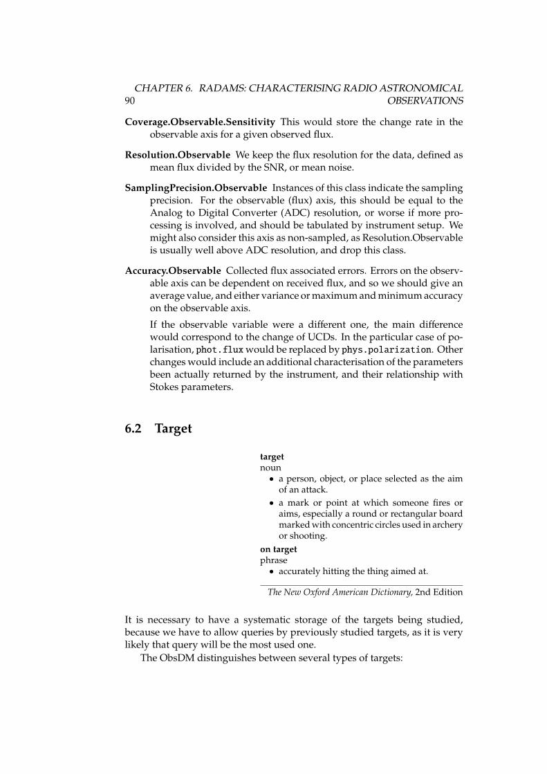
90CHAPTER 6. RADAMS: CHARACTERISING RADIO ASTRONOMICAL
OBSERVATIONS
Coverage.Observable.Sensitivity This would store the change rate in theobservable axis for a given observed flux.
Resolution.Observable We keep the flux resolution for the data, defined asmean flux divided by the SNR, or mean noise.
SamplingPrecision.Observable Instances of this class indicate the samplingprecision. For the observable (flux) axis, this should be equal to theAnalog to Digital Converter (ADC) resolution, or worse if more pro-cessing is involved, and should be tabulated by instrument setup. Wemight also consider this axis as non-sampled, as Resolution.Observableis usually well above ADC resolution, and drop this class.
Accuracy.Observable Collected flux associated errors. Errors on the observ-able axis can be dependent on received flux, and so we should give anaverage value, and either variance or maximum and minimum accuracyon the observable axis.
If the observable variable were a different one, the main differencewould correspond to the change of UCDs. In the particular case of po-larisation, phot.flux would be replaced by phys.polarization. Otherchanges would include an additional characterisation of the parametersbeen actually returned by the instrument, and their relationship withStokes parameters.
6.2 Target
targetnoun• a person, object, or place selected as the aim
of an attack.• a mark or point at which someone fires or
aims, especially a round or rectangular boardmarked with concentric circles used in archeryor shooting.
on targetphrase• accurately hitting the thing aimed at.
The New Oxford American Dictionary, 2nd Edition
It is necessary to have a systematic storage of the targets being studied,because we have to allow queries by previously studied targets, as it is verylikely that query will be the most used one.
The ObsDM distinguishes between several types of targets:
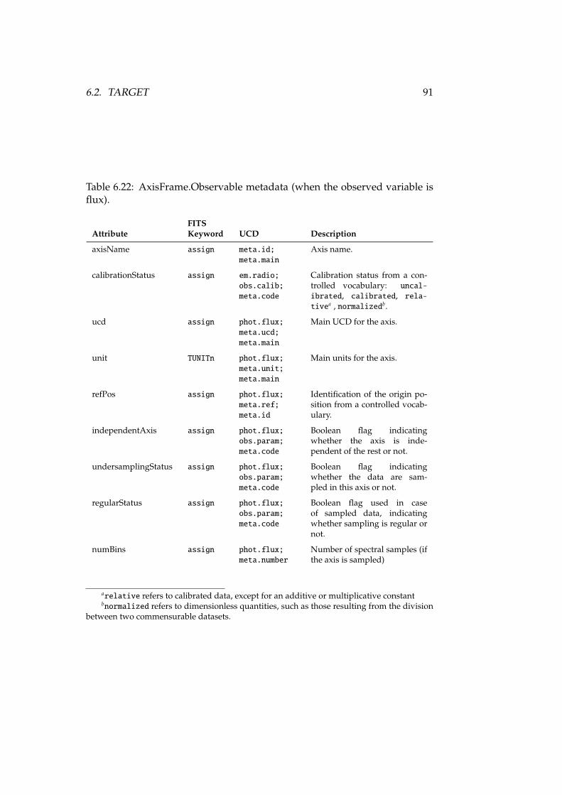
6.2. TARGET 91
Table 6.22: AxisFrame.Observable metadata (when the observed variable isflux).
FITSAttribute Keyword UCD Description
axisName assign meta.id;meta.main
Axis name.
calibrationStatus assign em.radio;obs.calib;meta.code
Calibration status from a con-trolled vocabulary: uncal-ibrated, calibrated, rela-tivea , normalizedb.
ucd assign phot.flux;meta.ucd;meta.main
Main UCD for the axis.
unit TUNITn phot.flux;meta.unit;meta.main
Main units for the axis.
refPos assign phot.flux;meta.ref;meta.id
Identification of the origin po-sition from a controlled vocab-ulary.
independentAxis assign phot.flux;obs.param;meta.code
Boolean flag indicatingwhether the axis is inde-pendent of the rest or not.
undersamplingStatus assign phot.flux;obs.param;meta.code
Boolean flag indicatingwhether the data are sam-pled in this axis or not.
regularStatus assign phot.flux;obs.param;meta.code
Boolean flag used in caseof sampled data, indicatingwhether sampling is regular ornot.
numBins assign phot.flux;meta.number
Number of spectral samples (ifthe axis is sampled)
arelative refers to calibrated data, except for an additive or multiplicative constantbnormalized refers to dimensionless quantities, such as those resulting from the division
between two commensurable datasets.

92CHAPTER 6. RADAMS: CHARACTERISING RADIO ASTRONOMICAL
OBSERVATIONS
Table 6.23: Coverage.Observable.Location metadata (when the observed vari-able is flux).
FITSAttribute Keyword UCD Description
coord.name assign phot.flux;meta.name
Name of the coordinate whose valuegoes in coord.value; in this case, fluxwith respect to refPos.
coord.value assign phot.flux;stat.max
Numeric value for the maximum flux(flux location).
Table 6.24: Coverage.Observable.Bounds metadata.
FITSAttribute Keyword UCD Description
coord.name assign phot.flux;meta.name
Name of the coordinate whose maxi-mum and minimum values go in co-ord.maxValue and coord.minValue.
coord.maxValue assign phot.flux;stat.max
Minimum flux value.
coord.minValue assign phot.flux;stat.min
Maximum flux value.
Table 6.25: Coverage.Observable.Support metadata (when the observed vari-able is flux).
FITSAttribute Keyword UCD Description
code assign em.radio;meta.record
Code for the interval where we willbe defining support; an array of [co-ord.code, startValue, endValue] tuplescan be used to define spectral support.
startValue assign em.freq;stat.min
Frequency interval start value.
endValue assign em.freq;stat.max
Frequency interval end value.
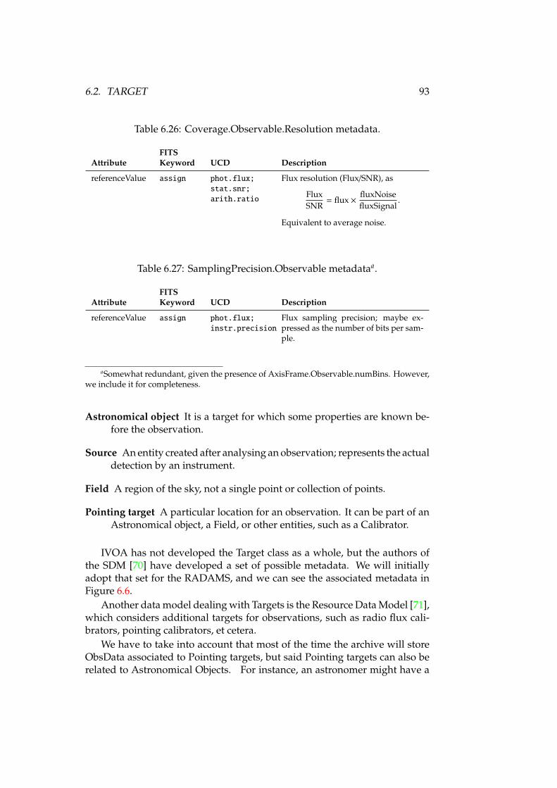
6.2. TARGET 93
Table 6.26: Coverage.Observable.Resolution metadata.
FITSAttribute Keyword UCD Description
referenceValue assign phot.flux;stat.snr;arith.ratio
Flux resolution (Flux/SNR), as
FluxSNR
= flux ×fluxNoisefluxSignal
.
Equivalent to average noise.
Table 6.27: SamplingPrecision.Observable metadataa.
FITSAttribute Keyword UCD Description
referenceValue assign phot.flux;instr.precision
Flux sampling precision; maybe ex-pressed as the number of bits per sam-ple.
aSomewhat redundant, given the presence of AxisFrame.Observable.numBins. However,we include it for completeness.
Astronomical object It is a target for which some properties are known be-fore the observation.
Source An entity created after analysing an observation; represents the actualdetection by an instrument.
Field A region of the sky, not a single point or collection of points.
Pointing target A particular location for an observation. It can be part of anAstronomical object, a Field, or other entities, such as a Calibrator.
IVOA has not developed the Target class as a whole, but the authors ofthe SDM [70] have developed a set of possible metadata. We will initiallyadopt that set for the RADAMS, and we can see the associated metadata inFigure 6.6.
Another data model dealing with Targets is the Resource Data Model [71],which considers additional targets for observations, such as radio flux cali-brators, pointing calibrators, et cetera.
We have to take into account that most of the time the archive will storeObsData associated to Pointing targets, but said Pointing targets can also berelated to Astronomical Objects. For instance, an astronomer might have a
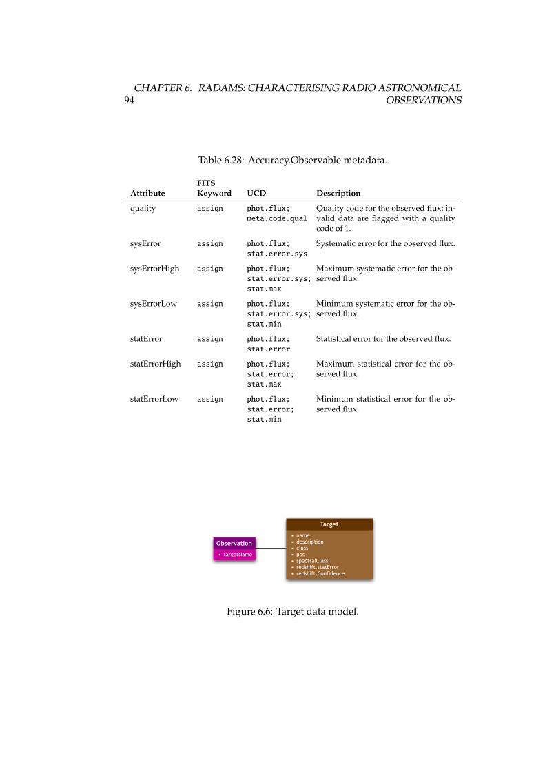
94CHAPTER 6. RADAMS: CHARACTERISING RADIO ASTRONOMICAL
OBSERVATIONS
Table 6.28: Accuracy.Observable metadata.
FITSAttribute Keyword UCD Description
quality assign phot.flux;meta.code.qual
Quality code for the observed flux; in-valid data are flagged with a qualitycode of 1.
sysError assign phot.flux;stat.error.sys
Systematic error for the observed flux.
sysErrorHigh assign phot.flux;stat.error.sys;stat.max
Maximum systematic error for the ob-served flux.
sysErrorLow assign phot.flux;stat.error.sys;stat.min
Minimum systematic error for the ob-served flux.
statError assign phot.flux;stat.error
Statistical error for the observed flux.
statErrorHigh assign phot.flux;stat.error;stat.max
Maximum statistical error for the ob-served flux.
statErrorLow assign phot.flux;stat.error;stat.min
Minimum statistical error for the ob-served flux.
• targetName
Observation• name• description• class• pos• spectralClass• redshift.statError• redshift.Confidence
Target
Figure 6.6: Target data model.
6.3. CONCLUSIONS 95
program in which s/he is looking for water masers as tracers of shocked re-gions, and specifies several Pointing targets. Those Pointing targets, however,will be most likely found within an Astronomical object, such as a planetarynebula. The association of the Astronomical object and the Pointing targetwill be made by means of the Target class.
6.3 Conclusions
In this chapter we have shown that the already specified IVOA data modelsfor Characterisation, together with the Target data model, do not need to bealtered in order to be used for radio astronomical archives.
However, the UCDs for data in the ObsDM, CharDM, or in the Targetclass had never been specified before, and this contributes to the better inter-operation of archives, as data with the same UCDs can be interesting for usein automatic data mining and data discovery.
In the next chapters we will analyse the parts of the RADAMS which needto be created in order to support radio astronomical archives.

Chapter 7
RADAMS: Curation, Packagingand Policy
In this chapter we will follow with our detailed description of the RADAMS,making emphasis on several classes which were introduced in the ObsDM,but which where not actually defined.
These classes are the Curation class, the Packaging class, and the Policyclass. There is still another class introduced by the ObsDM pending of def-inition, the Provenance class, but due to its relevance we will devote twoseparate chapters to it: one to the concept of Data Provenance in e-Science,and one to the actual implementation of Data Provenance in the RADAMS.
7.1 Curation
curatornoun• a keeper or custodian of a museum or other
collection.curateverb [trans.] (usu. be curated)• select, organize, and look after the items in
(a collection or exhibition): both exhibitions arecurated by the museum’s director.
The New Oxford American Dictionary, 2nd Edition
If we conceive sets of astronomical observations (for instance, a particularobservation program, a whole sky survey, et cetera) as collections or exhi-bitions, we can also generalise the VO concept (or any other data based e-Infrastructure) as a special kind of digital museum.
In that case, the definitions above point us to the fact that, for digital datacollections, Curation is related to:
97
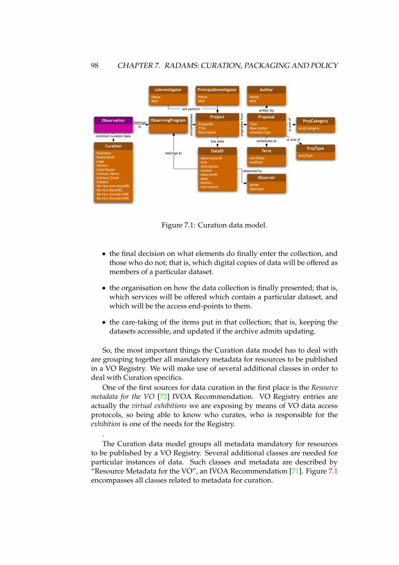
98 CHAPTER 7. RADAMS: CURATION, PACKAGING AND POLICY
Observation
-Publisher-PublisherID-Logo-Version-Contributor-Contact.Name-Contact.Email-Subject–Service.InterfaceURL-Service.BaseURL-Service.StandardURI-Service.StandardURL
Curation
-ProjectID-Title-Description
Project
-Name-Operator
Observer
-projCategory
ProjCategory
-projType
ProjType
-Title-Description-scheduleType
Proposal
-Name-Mail
Author
-startDate-endDate
Term
ObservingProgram
-observationID-title-description-creator-observerID-date-facility-instrument
DataID
-Name-Mail
PrincipalInvestigator
-Name-Mail
coInvestigator
common curation data
belongsto
enco
mpa
sses
has data
belongs to
observed by
orig
inat
es fr
om
written bywill perform
is one of
is on
e of
scheduled at
Figure 7.1: Curation data model.
• the final decision on what elements do finally enter the collection, andthose who do not; that is, which digital copies of data will be offered asmembers of a particular dataset.
• the organisation on how the data collection is finally presented; that is,which services will be offered which contain a particular dataset, andwhich will be the access end-points to them.
• the care-taking of the items put in that collection; that is, keeping thedatasets accessible, and updated if the archive admits updating.
So, the most important things the Curation data model has to deal withare grouping together all mandatory metadata for resources to be publishedin a VO Registry. We will make use of several additional classes in order todeal with Curation specifics.
One of the first sources for data curation in the first place is the Resourcemetadata for the VO [72] IVOA Recommendation. VO Registry entries areactually the virtual exhibitions we are exposing by means of VO data accessprotocols, so being able to know who curates, who is responsible for theexhibition is one of the needs for the Registry.
.The Curation data model groups all metadata mandatory for resources
to be published by a VO Registry. Several additional classes are needed forparticular instances of data. Such classes and metadata are described by“Resource Metadata for the VO”, an IVOA Recommendation [71]. Figure 7.1encompasses all classes related to metadata for curation.
7.1. CURATION 99
Observation The Observation class was discussed earlier. All observationsare related to a single Curation class.
Curation This is the main class that will group all curation related metadatawith relationships to complementary classes such as DataID and therest. It is the same for all data contained in the VO resource (archive)being described.
DataID There is an instance of this class for each different piece of data stored,or at least for each different way to store data. The Spectral Data Modeladvocates for this separation.
ObservingProgram Instances of this class keep common information aboutdifferent observations, describing its scientific or technical goals. Theyalso specify which is the project and/or proposal to which this observingprogram belongs. This class allows for easy querying by project or bycommon goals, such as maser surveys.
While there is debate about whether this class belongs to the Curationor to the Provenance Data Model, we believe it belongs to the CurationData Model, as it is an organisational unit, and in our view it has nothingto do with how the data were taken.
Project This class is the main class from an organizational point of view. Allobservations belong to a single project through a single proposal. AProject instance is related to a collection of Proposal instances.
Proposal As stated in the Project class, a Project can be divided in a seriesof Proposals. A Proposal instance can be related to one or more ob-servations. No observation can be related to more than one Proposalinstance.
Author An Author instance contains information about Proposal authors.
Observer Observer instances represent the observer/s assigned to a Proposal.It also contains a relationship with a Contact acting as the operator forthe instrument.
ProjCategory This instance specifies the scientific category of the project,from a controlled vocabulary; possible values, as specified by the Re-source Data Model, are: instrumental, galactic, terrestrial, so-larSystem, extragalactic, stellar. . .
ProjType This instance specifies the type of observation performed for aparticular proposal. Possible values are specified by the ResourceData Model, and form a controlled vocabulary that we have derivedfrom Lamb’s, ATNF and NRAO proposals [60, 59, 66]: astrometry,
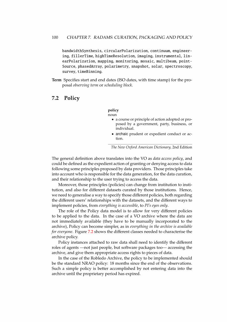
100 CHAPTER 7. RADAMS: CURATION, PACKAGING AND POLICY
bandwidthSynthesis, circularPolarization, continuum, engineer-ing, fillerTime, highTimeResolution, imaging, instrumental, lin-earPolarization, mapping, monitoring, mosaic, multibeam, point-Source, phasedArray, polarimetry, snapshot, solar, spectroscopy,survey, timeBinning.
Term Specifies start and end dates (ISO dates, with time stamp) for the pro-posal observing term or scheduling block.
7.2 Policy
policynoun• a course or principle of action adopted or pro-
posed by a government, party, business, orindividual.
• archaic prudent or expedient conduct or ac-tion.
The New Oxford American Dictionary, 2nd Edition
The general definition above translates into the VO as data access policy, andcould be defined as the expedient action of granting or denying access to datafollowing some principles proposed by data providers. Those principles takeinto account who is responsible for the data generation, for the data curation,and their relationship to the user trying to access the data.
Moreover, those principles (policies) can change from institution to insti-tution, and also for different datasets curated by those institutions. Hence,we need to generalise a way to specify those different policies, both regardingthe different users’ relationships with the datasets, and the different ways toimplement policies, from everything is accessible, to PI’s eyes only.
The role of the Policy data model is to allow for very different policiesto be applied to the data. In the case of a VO archive where the data arenot immediately available (they have to be manually incorporated to thearchive), Policy can become simpler, as in everything in the archive is availablefor everyone. Figure 7.2 shows the different classes needed to characterise thearchive policy.
Policy instances attached to raw data shall need to identify the differentroles of agents —not just people, but software packages too— accessing thearchive, and give them appropriate access rights to pieces of data.
In the case of the Robledo Archive, the policy to be implemented shouldbe the standard NRAO policy: 18 months since the end of the observations.Such a simple policy is better accomplished by not entering data into thearchive until the proprietary period has expired.
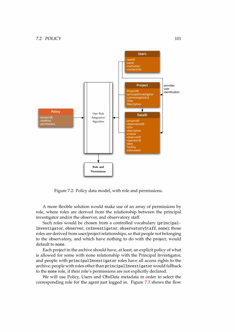
7.2. POLICY 101
+projectID-observationID-title-description-creator+observerID+operatorID-date-facility-instrument
DataID
-ProjectID+principalInvestigator+coInvestigator[n]-Title-Description
Project
-userID-name-institution-contactInfo
Users
+projectID-roleKind-permissions
Policy
providesuseridentification
User RoleAssignationAlgorithm
Role and Permissions
Figure 7.2: Policy data model, with role and permissions.
A more flexible solution would make use of an array of permissions byrole, where roles are derived from the relationship between the principalinvestigator and/or the observer, and observatory staff.
Such roles would be chosen from a controlled vocabulary (principal-Investigator, observer, coInvestigator, observatoryStaff, none); thoseroles are derived from user/project relationships, so that people not belongingto the observatory, and which have nothing to do with the project, woulddefault to none.
Each project in the archive should have, at least, an explicit policy of whatis allowed for some with none relationship with the Principal Investigator,and people with principalInvestigator roles have all access rights to thearchive; people with roles other than principalInvestigatorwould fallbackto the none role, if their role’s permissions are not explicitly declared.
We will use Policy, Users and ObsData metadata in order to select thecorresponding role for the agent just logged in. Figure 7.3 shows the flow
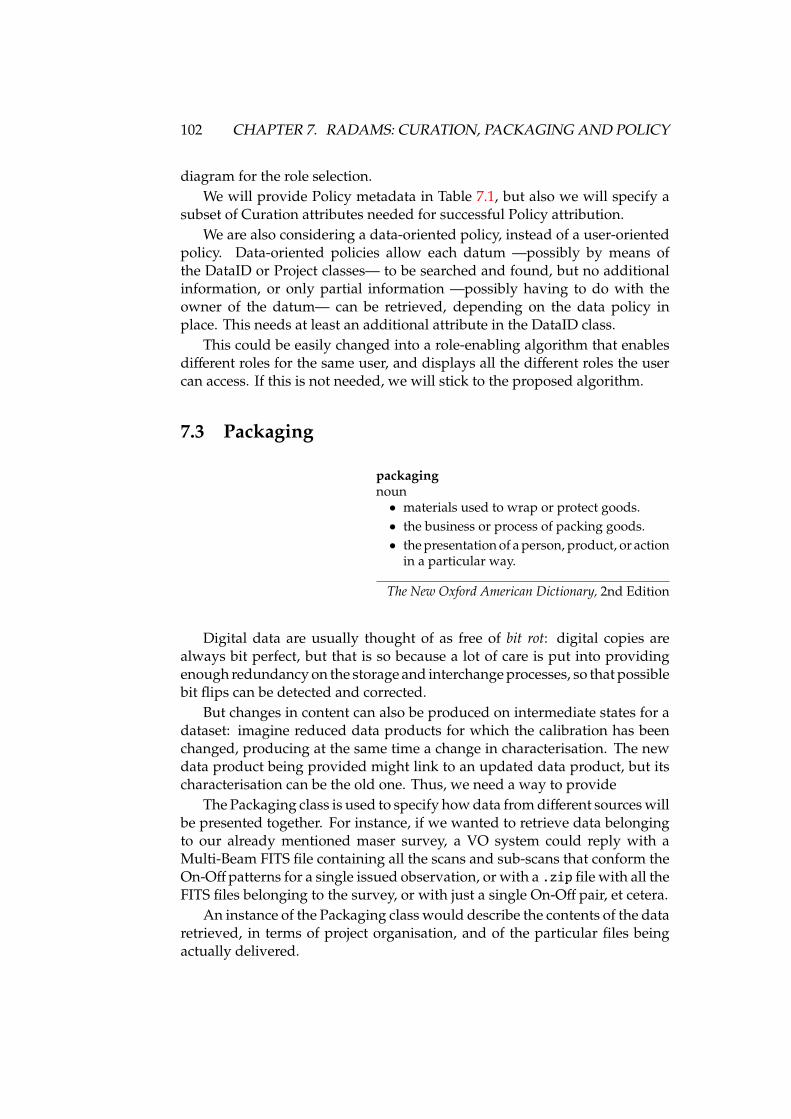
102 CHAPTER 7. RADAMS: CURATION, PACKAGING AND POLICY
diagram for the role selection.We will provide Policy metadata in Table 7.1, but also we will specify a
subset of Curation attributes needed for successful Policy attribution.We are also considering a data-oriented policy, instead of a user-oriented
policy. Data-oriented policies allow each datum —possibly by means ofthe DataID or Project classes— to be searched and found, but no additionalinformation, or only partial information —possibly having to do with theowner of the datum— can be retrieved, depending on the data policy inplace. This needs at least an additional attribute in the DataID class.
This could be easily changed into a role-enabling algorithm that enablesdifferent roles for the same user, and displays all the different roles the usercan access. If this is not needed, we will stick to the proposed algorithm.
7.3 Packaging
packagingnoun• materials used to wrap or protect goods.• the business or process of packing goods.• the presentation of a person, product, or action
in a particular way.
The New Oxford American Dictionary, 2nd Edition
Digital data are usually thought of as free of bit rot: digital copies arealways bit perfect, but that is so because a lot of care is put into providingenough redundancy on the storage and interchange processes, so that possiblebit flips can be detected and corrected.
But changes in content can also be produced on intermediate states for adataset: imagine reduced data products for which the calibration has beenchanged, producing at the same time a change in characterisation. The newdata product being provided might link to an updated data product, but itscharacterisation can be the old one. Thus, we need a way to provide
The Packaging class is used to specify how data from different sources willbe presented together. For instance, if we wanted to retrieve data belongingto our already mentioned maser survey, a VO system could reply with aMulti-Beam FITS file containing all the scans and sub-scans that conform theOn-Off patterns for a single issued observation, or with a .zip file with all theFITS files belonging to the survey, or with just a single On-Off pair, et cetera.
An instance of the Packaging class would describe the contents of the dataretrieved, in terms of project organisation, and of the particular files beingactually delivered.
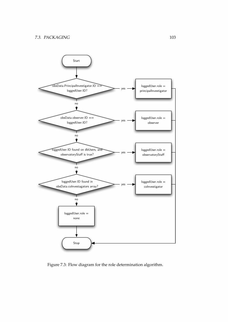
7.3. PACKAGING 103
Start
Stop
obsData.PrincipalInvestigator.ID == loggedUser.ID?
loggedUser.role =principalInvestigator
obsData.observer.ID == loggedUser.ID?
loggedUser.role =observer
loggedUser.ID found in obsData.coInvestagators array?
loggedUser.role =coInvestigator
loggedUser.ID found on dbUsers, and observatoryStaff is true?
loggedUser.role =observatoryStaff
loggedUser.role =none
yes
no
yes
yes
yes
no
no
no
Figure 7.3: Flow diagram for the role determination algorithm.
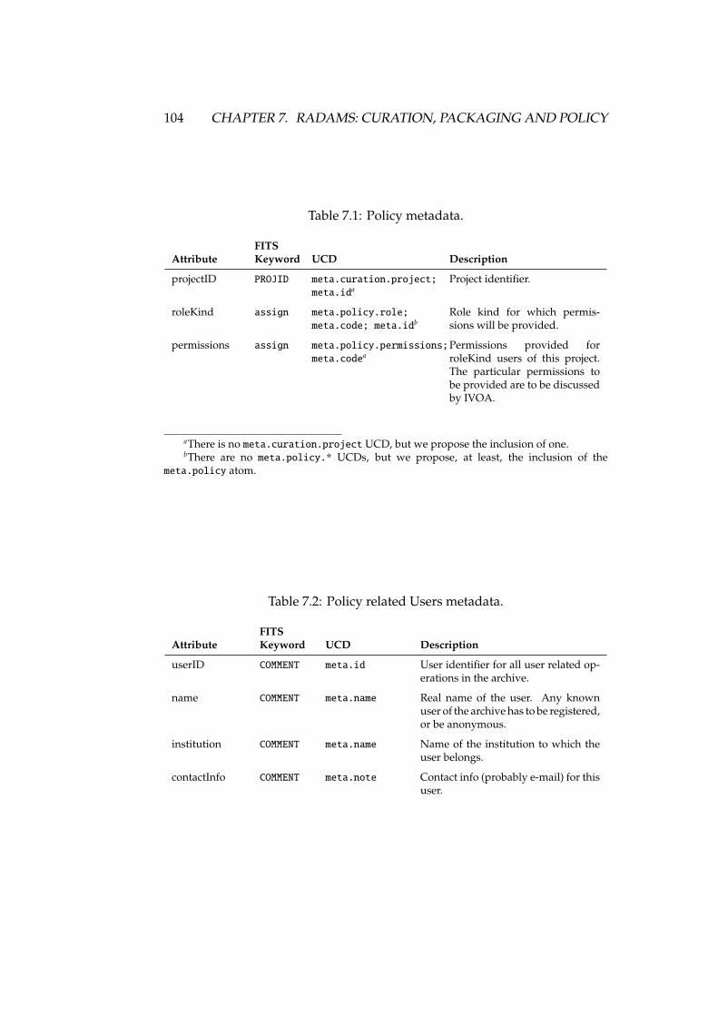
104 CHAPTER 7. RADAMS: CURATION, PACKAGING AND POLICY
Table 7.1: Policy metadata.
FITSAttribute Keyword UCD Description
projectID PROJID meta.curation.project;meta.ida
Project identifier.
roleKind assign meta.policy.role;meta.code; meta.idb
Role kind for which permis-sions will be provided.
permissions assign meta.policy.permissions;meta.codea
Permissions provided forroleKind users of this project.The particular permissions tobe provided are to be discussedby IVOA.
aThere is no meta.curation.project UCD, but we propose the inclusion of one.bThere are no meta.policy.* UCDs, but we propose, at least, the inclusion of the
meta.policy atom.
Table 7.2: Policy related Users metadata.
FITSAttribute Keyword UCD Description
userID COMMENT meta.id User identifier for all user related op-erations in the archive.
name COMMENT meta.name Real name of the user. Any knownuser of the archive has to be registered,or be anonymous.
institution COMMENT meta.name Name of the institution to which theuser belongs.
contactInfo COMMENT meta.note Contact info (probably e-mail) for thisuser.
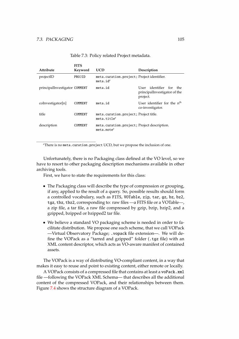
7.3. PACKAGING 105
Table 7.3: Policy related Project metadata.
FITSAttribute Keyword UCD Description
projectID PROJID meta.curation.project;meta.ida
Project identifier.
principalInvestigator COMMENT meta.id User identifier for theprincipalInvestigator of theproject.
coInvestigator[n] COMMENT meta.id User identifier for the nth
co-investigator.
title COMMENT meta.curation.project;meta.titlea
Project title.
description COMMENT meta.curation.project;meta.notea
Project description.
aThere is no meta.curation.project UCD, but we propose the inclusion of one.
Unfortunately, there is no Packaging class defined at the VO level, so wehave to resort to other packaging description mechanisms available in otherarchiving tools.
First, we have to state the requirements for this class:
• The Packaging class will describe the type of compression or grouping,if any, applied to the result of a query. So, possible results should forma controlled vocabulary, such as FITS, VOTable, zip, tar, gz, bz, bz2,tgz, tbz, tbz2, corresponding to: raw files —a FITS file or a VOTable—,a zip file, a tar file, a raw file compressed by gzip, bzip, bzip2, and agzipped, bzipped or bzipped2 tar file.
• We believe a standard VO packaging scheme is needed in order to fa-cilitate distribution. We propose one such scheme, that we call VOPack—Virtual Observatory Package; .vopack file extension—. We will de-fine the VOPack as a “tarred and gzipped” folder (.tgz file) with anXML content descriptor, which acts as VO-aware manifest of containedassets.
The VOPack is a way of distributing VO-compliant content, in a way thatmakes it easy to reuse and point to existing content, either remote or locally.
A VOPack consists of a compressed file that contains at least a voPack.xmlfile —following the VOPack XML Schema— that describes all the additionalcontent of the compressed VOPack, and their relationships between them.Figure 7.4 shows the structure diagram of a VOPack.
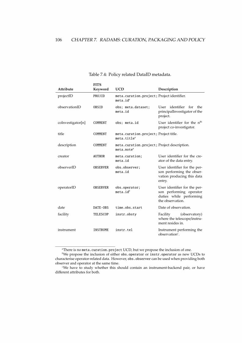
106 CHAPTER 7. RADAMS: CURATION, PACKAGING AND POLICY
Table 7.4: Policy related DataID metadata.
FITSAttribute Keyword UCD Description
projectID PROJID meta.curation.project;meta.ida
Project identifier.
observationID OBSID obs; meta.dataset;meta.id
User identifier for theprincipalInvestigator of theproject.
coInvestigator[n] COMMENT obs; meta.id User identifier for the nth
project co-investigator.
title COMMENT meta.curation.project;meta.titlea
Project title.
description COMMENT meta.curation.project;meta.notea
Project description.
creator AUTHOR meta.curation;meta.id
User identifier for the cre-ator of the data entry.
observerID OBSERVER obs.observer;meta.id
User identifier for the per-son performing the obser-vation producing this dataentry.
operatorID OBSERVER obs.operator;meta.idb
User identifier for the per-son performing operatorduties while performingthe observation.
date DATE-OBS time.obs.start Date of observation.
facility TELESCOP instr.obsty Facility (observatory)where the telescope/instru-ment resides in.
instrument INSTRUME instr.tel Instrument performing theobservationc.
aThere is no meta.curation.project UCD, but we propose the inclusion of one.bWe propose the inclusion of either obs.operator or instr.operator as new UCDs to
characterise operator-related data. However, obs.observer can be used when providing bothobserver and operator at the same time.
cWe have to study whether this should contain an instrument-backend pair, or havedifferent attributes for both.
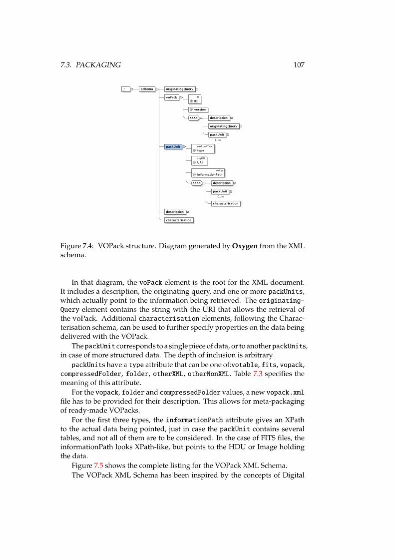
7.3. PACKAGING 107
/ schema originatingQuery
voPack@
IDID
@ version
description
originatingQuery
packUnit1..
packUnit@
packUnitTypetype
@anyURIURI
@string
informationPath
description
packUnit0..
characterisation
description
characterisation
Figure 7.4: VOPack structure. Diagram generated by Oxygen from the XMLschema.
In that diagram, the voPack element is the root for the XML document.It includes a description, the originating query, and one or more packUnits,which actually point to the information being retrieved. The originating-Query element contains the string with the URI that allows the retrieval ofthe voPack. Additional characterisation elements, following the Charac-terisation schema, can be used to further specify properties on the data beingdelivered with the VOPack.
ThepackUnit corresponds to a single piece of data, or to anotherpackUnits,in case of more structured data. The depth of inclusion is arbitrary.
packUnits have a type attribute that can be one of:votable, fits, vopack,compressedFolder, folder, otherXML, otherNonXML. Table 7.3 specifies themeaning of this attribute.
For the vopack, folder and compressedFolder values, a new vopack.xmlfile has to be provided for their description. This allows for meta-packagingof ready-made VOPacks.
For the first three types, the informationPath attribute gives an XPathto the actual data being pointed, just in case the packUnit contains severaltables, and not all of them are to be considered. In the case of FITS files, theinformationPath looks XPath-like, but points to the HDU or Image holdingthe data.
Figure 7.5 shows the complete listing for the VOPack XML Schema.The VOPack XML Schema has been inspired by the concepts of Digital
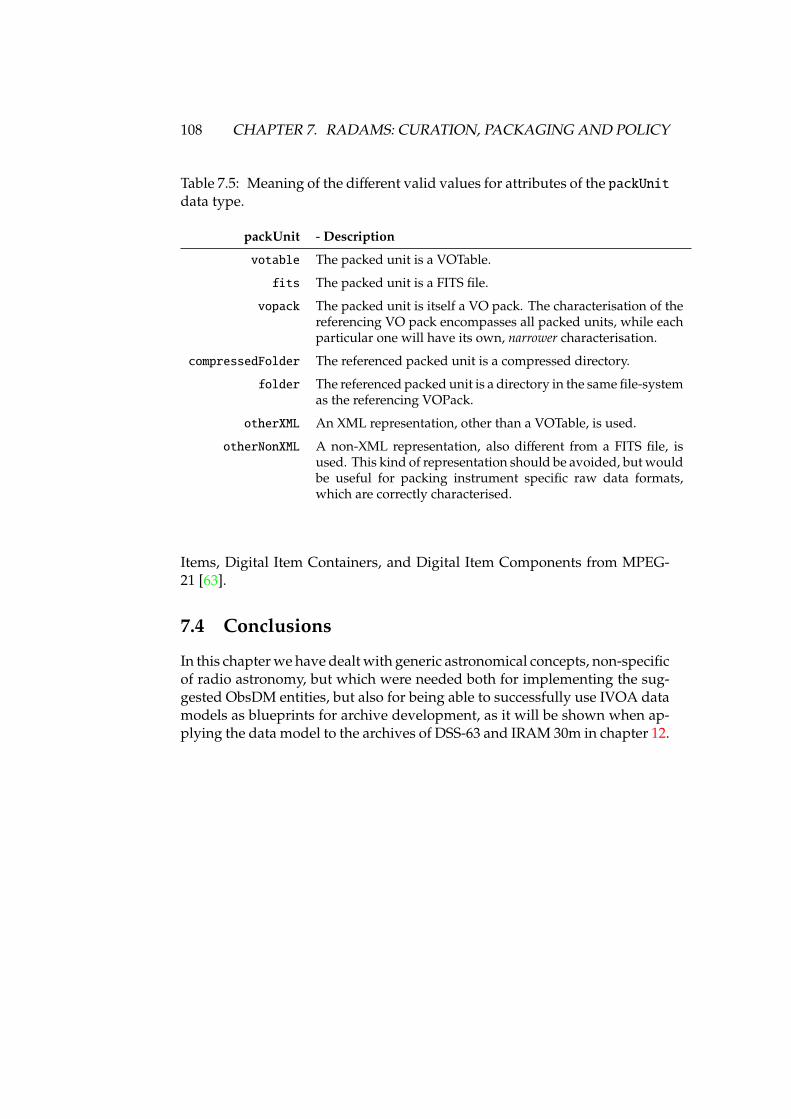
108 CHAPTER 7. RADAMS: CURATION, PACKAGING AND POLICY
Table 7.5: Meaning of the different valid values for attributes of the packUnitdata type.
packUnit - Description
votable The packed unit is a VOTable.
fits The packed unit is a FITS file.
vopack The packed unit is itself a VO pack. The characterisation of thereferencing VO pack encompasses all packed units, while eachparticular one will have its own, narrower characterisation.
compressedFolder The referenced packed unit is a compressed directory.
folder The referenced packed unit is a directory in the same file-systemas the referencing VOPack.
otherXML An XML representation, other than a VOTable, is used.
otherNonXML A non-XML representation, also different from a FITS file, isused. This kind of representation should be avoided, but wouldbe useful for packing instrument specific raw data formats,which are correctly characterised.
Items, Digital Item Containers, and Digital Item Components from MPEG-21 [63].
7.4 Conclusions
In this chapter we have dealt with generic astronomical concepts, non-specificof radio astronomy, but which were needed both for implementing the sug-gested ObsDM entities, but also for being able to successfully use IVOA datamodels as blueprints for archive development, as it will be shown when ap-plying the data model to the archives of DSS-63 and IRAM 30m in chapter 12.
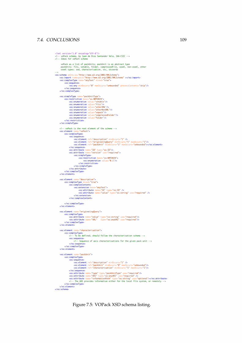
7.4. CONCLUSIONS 109
<?xml version="1.0" encoding="UTF-8"?>
<!-- voPack schema, by Juan de Dios Santander Vela, IAA-CSIC -->
<!-- Ideas for voPach schema
voPack as a list of packUnits; packUnit is an abstract type
packUnits: fits, votable, folder, compressedFile, voxml, non-voxml, other
voxml types: sed, characterisation, stc, stcoords
-->
<xs:schema xmlns:xs="http://www.w3.org/2001/XMLSchema">
<xs:import namespace="http://www.w3.org/2001/XMLSchema" ></xs:import>
<xs:complexType name="anyText" mixed="true">
<xs:sequence>
<xs:any minOccurs="0" maxOccurs="unbounded" processContents="skip"/>
</xs:sequence>
</xs:complexType>
<xs:simpleType name="packUnitType">
<xs:restriction base="xs:NMTOKEN">
<xs:enumeration value="votable"/>
<xs:enumeration value="fits"/>
<xs:enumeration value="otherXML"/>
<xs:enumeration value="otherNonXML"/>
<xs:enumeration value="vopack"/>
<xs:enumeration value="compressedFolder"/>
<xs:enumeration value="folder"/>
</xs:restriction>
</xs:simpleType>
<!-- voPack is the root element of the schema -->
<xs:element name="voPack">
<xs:complexType>
<xs:sequence>
<xs:element ref="description" minOccurs="1" />
<xs:element ref="originatingQuery" minOccurs="1" maxOccurs="1"/>
<xs:element ref="packUnit" minOccurs="1" maxOccurs="unbounded"></xs:element>
</xs:sequence>
<xs:attribute name="ID" type="xs:ID"/>
<xs:attribute name="version" use="required">
<xs:simpleType>
<xs:restriction base="xs:NMTOKEN">
<xs:enumeration value="0.1"/>
</xs:restriction>
</xs:simpleType>
</xs:attribute>
</xs:complexType>
</xs:element>
<xs:element name="description">
<xs:complexType mixed="true">
<xs:complexContent>
<xs:extension base="anyText">
<xs:attribute name="ID" type="xs:ID" />
<xs:attribute name="value" type="xs:string" use="required" />
</xs:extension>
</xs:complexContent>
</xs:complexType>
</xs:element>
<xs:element name="originatingQuery">
<xs:complexType>
<xs:attribute name="value" type="xs:string" use="required"/>
<xs:attribute name="URL" type="xs:anyURI" use="required"/>
</xs:complexType>
</xs:element>
<xs:element name="characterisation">
<xs:complexType>
<!-- To be defined; should follow the characterisation schema -->
<xs:sequence>
<!-- Sequence of axis characterisations for the given pack unit -->
</xs:sequence>
</xs:complexType>
</xs:element>
<xs:element name="packUnit">
<xs:complexType>
<xs:sequence>
<xs:element ref="description" minOccurs="1" />
<xs:element ref="packUnit" minOccurs="0" maxOccurs="unbounded"/>
<xs:element ref="characterisation" minOccurs="1" maxOccurs="1"/>
</xs:sequence>
<xs:attribute name="type" type="packUnitType" use="required"/>
<xs:attribute name="URI" type="xs:anyURI" use="required" />
<xs:attribute name="informationPath" type="xs:string" use="optional"></xs:attribute>
<!-- The URI provides information either for the local file system, or remotely -->
</xs:complexType>
</xs:element>
</xs:schema>
Figure 7.5: VOPack XSD schema listing.

Chapter 8
Data Provenance
provenancenoun• the place of origin or earliest known history of
something.• the beginning of something’s existence; some-
thing’s origin.• a record of ownership of a work of art or an an-
tique, used as a guide to authenticity or qual-ity.
The New Oxford American Dictionary, 2nd Edition
The dictionary definition above points to the main three elements to whichdata provenance in e-Science has to deal with: Attribution, i.e. proper ac-knowledgement of authorship and or origin; Data Quality; and Replicationof results, i.e., the chain of processes needed to derive a result, beginning withdata sources.
In the VO context, we can synthesise a definition by stating that Prove-nance (data provenance) is the record of the earliest known history of anastronomical data set, to be used as a guide to data quality and of data own-ership.
Astronomical datasets use the data coming from different photons1 toderive physical properties from the observed objects. Therefore, data prove-nance —also known as lineage information— in astrophysics is, in fact, theanswer to the question What was done to this collection of photons, and whichsystems did it?
1Their arrival rate, their energy distribution, the positions from the sky, the differencewith properties of photons not coming from the observed region; in addition, the response tophotons, and to their absence, has also to be determined.
111
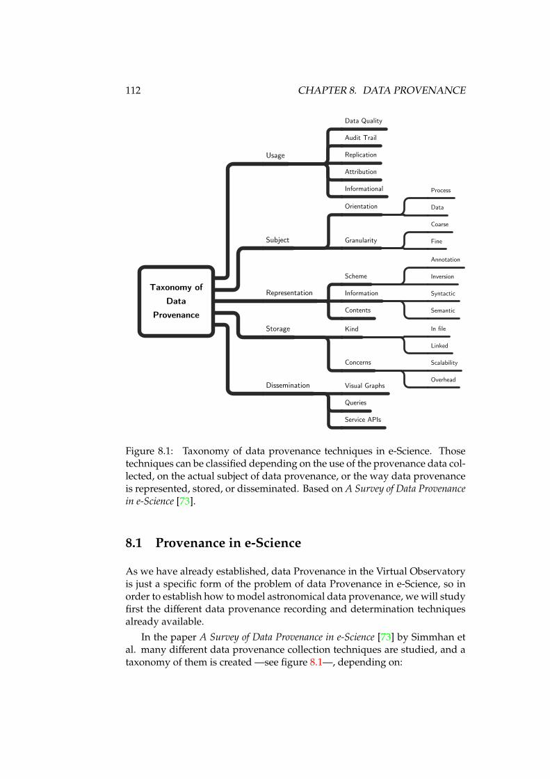
112 CHAPTER 8. DATA PROVENANCE
Taxonomy of Data
Provenance
Usage
Data Quality
Audit Trail
Replication
Attribution
Informational
Subject
Orientation
Process
Data
Granularity
Coarse
Fine
Representation
Scheme
Annotation
Inversion
Information Syntactic
SemanticContents
Storage Kind In file
Linked
Concerns Scalability
OverheadDissemination Visual Graphs
Queries
Service APIs
Figure 8.1: Taxonomy of data provenance techniques in e-Science. Thosetechniques can be classified depending on the use of the provenance data col-lected, on the actual subject of data provenance, or the way data provenanceis represented, stored, or disseminated. Based on A Survey of Data Provenancein e-Science [73].
8.1 Provenance in e-Science
As we have already established, data Provenance in the Virtual Observatoryis just a specific form of the problem of data Provenance in e-Science, so inorder to establish how to model astronomical data provenance, we will studyfirst the different data provenance recording and determination techniquesalready available.
In the paper A Survey of Data Provenance in e-Science [73] by Simmhan etal. many different data provenance collection techniques are studied, and ataxonomy of them is created —see figure 8.1—, depending on:
8.1. PROVENANCE IN E-SCIENCE 113
Usage Data provenance information can be used for estimating data qualityand data reliability, or to provide an audit trail of the data transforma-tions. It can also be used to replicate an experiment, to attribute thecreation of a dataset to a set of original (in the sense of originating) data,and to the set of processes needed to derive the new dataset. Or it canbe informational, without providing enough information to assess anyof the above.
Subject Data provenance can be focused on the data themselves, collectinglineage metadata from each data product, or on the processes on thedata. And in any case the recorded provenance can be coarse grained(for instance, describing a whole set of data) or fine grained (describ-ing each single datum and/or process; for instance, database tuples’attributes).
Representation The way data provenance can be represented is also diverse,and some of them depend on the processing system being studied. Thetwo main approaches in the literature are annotations and inversion.Annotations are a priori provenance metadata: the transformed data areaccompanied by provenance metadata which has been created prior tothe transformation. On the other hand, inversion data provenance is cre-ated a posteriori from the data products of a transformation which can beinverted, with provenance metadata being created from the documen-tation of the process and the differences between inputs and outputs.It is clear that inversion metadata are more compact, while annotationscan include parameters of processes, their versions, and even referencesto publications.
As some of the lineage information implies relationships between datasetsand processes, that information can be captured in data models aboutthe processes, or using semantic web technologies, such as the RDF andOWL languages, in order to describe such relationships. In this way,the process semantics are documented. In any case, the process syntaxis specified from the input data, the output data, and annotations, ifpresent.
Storage As provenance metadata can be generated, collected and/or trans-mitted at many different places, there must be a way to keep thosemetadata stored, while keeping the relationship with the data them-selves. Depending on the grain of the metadata collection process, andon whether the lineage information is just updated or versioned, theamount of provenance metadata can grow several orders of magnitudeabove the original data. Both the overhead of provenance metadata(percentage of storage devoted to provenance versus data, and cost ofmetadata management), and the scalability of the system, that is, how
114 CHAPTER 8. DATA PROVENANCE
to deal with the provenance metadata if the data rate increases an orderof magnitude.
Dissemination Finally, provenance metadata are gathered for applicationsto use them. Typical ways of disseminating lineage information are bymeans of derivation graphs , but in many cases where the provenancemetadata are stored inline with the data the form is just a list of time-stamped annotations. If semantic web tools are used, workflows candetermine the input provenance information and create the dissemi-nation graph at runtime. In addition, specially in cases were lineagemetadata are stored in databases or XML documents, provenance spe-cific queries can be performed, and even provenance query APIs can becreated so that different systems can access such information.
Another classification [74] of Provenance data can be performed regardinghow it is collected or computed:
Why provenance Refers to the reason why a datum is in a given dataset, i.e.,the query that was performed, including data sources. For data comingfrom database queries, different fields can have different sources, butall fields, and many rows derived from the same query, will share thatquery. In a sense, Why provenance is a proof that a datum belongs toa processed (queried) data set, as it corresponds to the minimum setof sources and sources’ entries which, together with the query beingperformed, will provide that datum as an answer.
Where provenance Refers to the actual progenitors of each particular datum,i.e., what particular database tuple, and field in the tuple, provided thedatum we are analysing.
The difference between both kinds can be better illustrated using a data-base originated example. Let us imagine the SQL query:
SELECT name, telephoneFROM employeeWHERE salary > (SELECT AVERAGE salary FROM employee)
And let us say one of the tuples in the result is ("John Doe", 555123467).As all rows inemployeewhere needed for the calculation of the salary average,a change in any row could make our target tuple disappear from the resultlist, so the Why provenance is the query plus the salary, name and telephonefields of all rows of the employee table. The Where provenance, however, isonly concerned with the actual progenitor of each of the tuple’s datum, andthe answer is the name and employee fields of the row containing John Doe’sentry in the employee table.
Finally, another difference can be established for data provenance collec-tion systems, depending on the data collection strategy:

8.2. PROVENANCE IN ASTRONOMY AND ASTROPHYSICS 115
Eager collection Lineage information is created/computed after each trans-formational or derivational step.
Lazy collection Provenance information is calculated on demand, using spe-cific knowledge of the transformations, and parameters saved.
We will end up our review of data provenance systems and classificationsby showing table 8.1 of different data provenance management systems indifferent application areas, and see their characteristics.
We can see that most of the systems assume a relational database infras-tructure, and rely on annotations for carrying on provenance information.Only systems completely contained within a relational database systems useinverse queries or functions for their recovery of data provenance.
So, in order to establish a Data Provenance framework for the VirtualObservatory we will have to establish all of the items above: how to collectthe information, which will be the intended use, and how is the informationgoing to be represented, stored, and presented to intended users and systems;whether we need a Why or Where provenance system depending on typicalVO use cases; and if such system must be Eager or Lazy, again depending onuse cases.
8.2 Provenance in astronomy and astrophysics
After the classification above, we will study the different data provenancetechniques in use within the astronomy, together with their intended appli-cation.
Typically, one of the uses of header cards in FITS files is storing COMMENTSand HISTORY cards. Figure 8.2 shows an example of a FITS file processed bythe AIPS2 interferometric data reduction software.
In that figure we can see an example of how typical astrophysical toolshave been dealing with data provenance. Each different application can makeuse of the FITS header cards, specifically of the HISTORY keyword, in order toprovide feedback of the steps being performed on the data.
In this case, the data provenance being provided is of the Why kind, albeitnot complete. Apart from the text annotation on the FITS headers, tablesof task Parameters are stored within the FITS file itself, so this provenanceinformation is collected eagerly, and corresponds to Why provenance. If allthe operations where invertible, it would also provide an invertible Whereprovenance, but some of the data is lost during each processing step.
However, that is the case for a particular package. The FITS headersadded by the difmap package3, for example, only indicate that difmap hastouched the file somehow, without any details:
2http://www.aips.nrao.edu/3ftp://ftp.astro.caltech.edu/pub/difmap/difmap.html
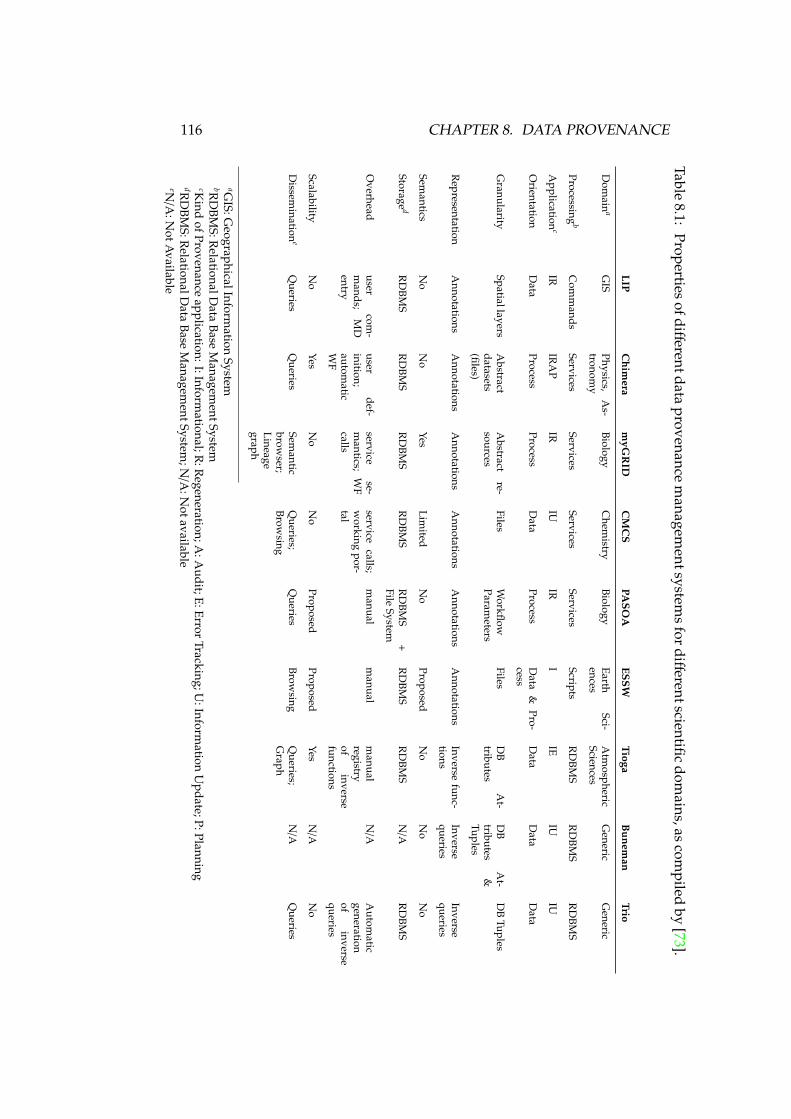
116 CHAPTER 8. DATA PROVENANCETable
8.1:Properties
ofdifferentdataprovenance
managem
entsystems
fordifferentscientific
domains,as
compiled
by[73].
LIPC
himera
myG
RID
CM
CS
PASO
AESSW
TiogaB
uneman
Trio
Dom
aina
GIS
Physics,A
s-tronom
yBiology
Chem
istryBiology
EarthSci-
encesA
tmospheric
SciencesG
enericG
eneric
Processingb
Com
mands
ServicesServices
ServicesServices
ScriptsR
DBM
SR
DBM
SR
DBM
S
Application
cIR
IRA
PIR
IUIR
IIE
IUIU
Orientation
Data
ProcessProcess
Data
ProcessD
ata&
Pro-cess
Data
Data
Data
Granularity
SpatiallayersA
bstractdatasets(files)
Abstract
re-sources
FilesW
orkflowParam
etersFiles
DB
At-
tributesD
BA
t-tributes
&Tuples
DB
Tuples
Representation
Annotations
Annotations
Annotations
Annotations
Annotations
Annotations
Inversefunc-
tionsInversequeries
Inversequeries
Semantics
No
No
YesLim
itedN
oProposed
No
No
No
Storaged
RD
BMS
RD
BMS
RD
BMS
RD
BMS
RD
BMS
+File
SystemR
DBM
SR
DBM
SN
/AR
DBM
S
Overhead
usercom
-m
ands;M
Dentry
userdef-
inition;autom
aticW
F
servicese-
mantics;
WF
calls
servicecalls;
working
por-tal
manual
manual
manual
registryof
inversefunctions
N/A
Autom
aticgenerationof
inversequeries
ScalabilityN
oYes
No
No
ProposedProposed
YesN
/AN
o
Dissem
inatione
Queries
Queries
Semantic
browser;
Lineagegraph
Queries;
Browsing
Queries
Browsing
Queries;
Graph
N/A
Queries
aGIS:G
eographicalInformation
SystembR
DBM
S:RelationalD
ataBase
Managem
entSystemcK
indofProvenance
application:I:Informational;R
:Regeneration;A
:Audit;E:Error
Tracking;U:Inform
ationU
pdate;P:PlanningdR
DBM
S:RelationalD
ataBase
Managem
entSystem;N
/A:N
otavailableeN
/A:N
otAvailable
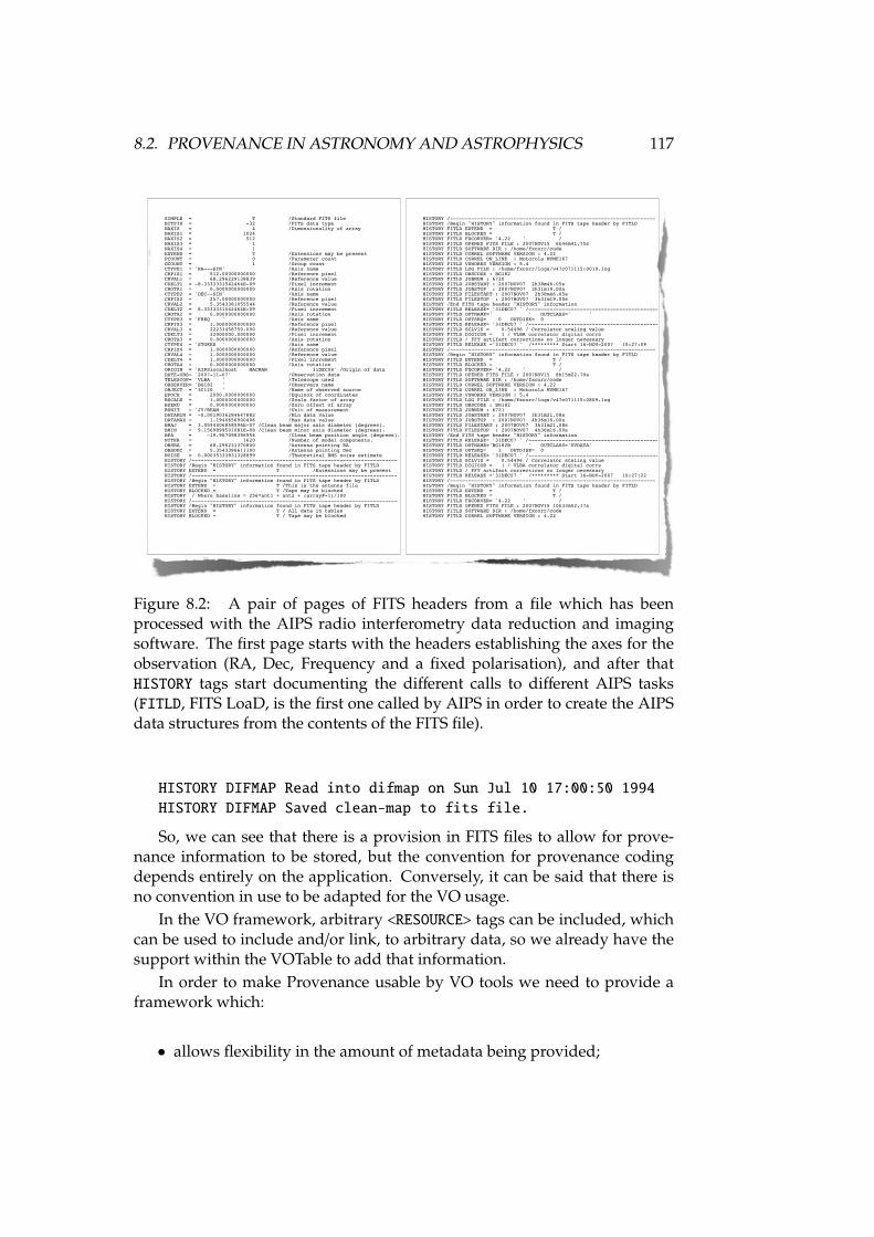
8.2. PROVENANCE IN ASTRONOMY AND ASTROPHYSICS 117
SIMPLE = T /Standard FITS file BITPIX = -32 /FITS data type NAXIS = 4 /Dimensionality of array NAXIS1 = 1024 NAXIS2 = 512 NAXIS3 = 1 NAXIS4 = 1 EXTEND = T /Extensions may be present PCOUNT = 0 /Parameter count GCOUNT = 1 /Group count CTYPE1 = 'RA---SIN' /Axis name CRPIX1 = 512.00000000000 /Reference pixel CRVAL1 = 68.296229138839 /Reference value CDELT1 = -8.3333331542464E-09 /Pixel increment CROTA1 = 0.0000000000000 /Axis rotation CTYPE2 = 'DEC--SIN' /Axis name CRPIX2 = 257.00000000000 /Reference pixel CRVAL2 = 5.3543381055544 /Reference value CDELT2 = 8.3333331542464E-09 /Pixel increment CROTA2 = 0.0000000000000 /Axis rotation CTYPE3 = 'FREQ ' /Axis name CRPIX3 = 1.0000000000000 /Reference pixel CRVAL3 = 22233458750.000 /Reference value CDELT3 = 32000000.000000 /Pixel increment CROTA3 = 0.0000000000000 /Axis rotation CTYPE4 = 'STOKES ' /Axis name CRPIX4 = 1.0000000000000 /Reference pixel CRVAL4 = 1.0000000000000 /Reference value CDELT4 = 1.0000000000000 /Pixel increment CROTA4 = 0.0000000000000 /Axis rotation ORIGIN = 'AIPSlocalhost MACMAR 31DEC08' /Origin of data DATE-OBS= '2007-11-07' /Observation date TELESCOP= 'VLBA ' /Telescope used OBSERVER= 'BG182 ' /Observers name OBJECT = '3C120 ' /Name of observed source EPOCH = 2000.0000000000 /Equinox of coordinates BSCALE = 1.0000000000000 /Scale factor of array BZERO = 0.0000000000000 /Zero offset of array BUNIT = 'JY/BEAM ' /Unit of measurement DATAMIN = -0.0019036284647882 /Min data value DATAMAX = 1.1940656900406 /Max data value BMAJ = 3.0594406858596E-07 /Clean beam major axis diameter (degrees). BMIN = 9.1569899501081E-08 /Clean beam minor axis diameter (degrees). BPA = -19.967098396954 /Clean beam position angle (degrees). NITER = 1620 /Number of model components. OBSRA = 68.296231370800 /Antenna pointing RA OBSDEC = 5.3543386611100 /Antenna pointing Dec NOISE = 0.00035333831328899 /Theoretical RMS noise estimate HISTORY /-------------------------------------------------------------------- HISTORY /Begin "HISTORY" information found in FITS tape header by FITLD HISTORY EXTEND = T /Extensions may be present HISTORY /-------------------------------------------------------------------- HISTORY /Begin "HISTORY" information found in FITS tape header by FITLD HISTORY EXTEND = T /This is the antenna file HISTORY BLOCKED = T /Tape may be blocked HISTORY / Where baseline = 256*ant1 + ant2 + (array#-1)/100 HISTORY /-------------------------------------------------------------------- HISTORY /Begin "HISTORY" information found in FITS tape header by FITLD HISTORY EXTEND = T / All data in tables HISTORY BLOCKED = T / Tape may be blocked
HISTORY /-------------------------------------------------------------------- HISTORY /Begin "HISTORY" information found in FITS tape header by FITLD HISTORY FITLD EXTEND = T / HISTORY FITLD BLOCKED = T / HISTORY FITLD FXCORVER= '4.22 ' / HISTORY FITLD OPENED FITS FILE : 2007NOV15 6h46m41.75s HISTORY FITLD SOFTWARE DIR : /home/fxcorr/code HISTORY FITLD CORREL SOFTWARE VERSION : 4.22 HISTORY FITLD CORREL ON_LINE : Motorola MVME167 HISTORY FITLD VXWORKS VERSION : 5.4 HISTORY FITLD LOG FILE : /home/fxcorr/logs/v47c071115:0019.log HISTORY FITLD OBSCODE : BG182 HISTORY FITLD JOBNUM : 6720 HISTORY FITLD JOBSTART : 2007NOV07 2h38m46.05s HISTORY FITLD JOBSTOP : 2007NOV07 3h31m19.00s HISTORY FITLD FILESTART : 2007NOV07 2h38m46.05s HISTORY FITLD FILESTOP : 2007NOV07 3h31m19.00s HISTORY /End FITS tape header "HISTORY" information HISTORY FITLD RELEASE= '31DEC07 ' /-------------------------------------------- HISTORY FITLD OUTNAME=' ' OUTCLASS=' ' HISTORY FITLD OUTSEQ= 0 OUTDISK= 0 HISTORY FITLD RELEASE= '31DEC07 ' /-------------------------------------------- HISTORY FITLD SCLVIS = 0.54496 / Correlator scaling value HISTORY FITLD DIGICOR = 1 / VLBA correlator digital corrs HISTORY FITLD / FFT artifact corrections no longer necessary HISTORY FITLD RELEASE ='31DEC07 ' /********* Start 16-NOV-2007 10:27:09 HISTORY /-------------------------------------------------------------------- HISTORY /Begin "HISTORY" information found in FITS tape header by FITLD HISTORY FITLD EXTEND = T / HISTORY FITLD BLOCKED = T / HISTORY FITLD FXCORVER= '4.22 ' / HISTORY FITLD OPENED FITS FILE : 2007NOV15 8h15m22.70s HISTORY FITLD SOFTWARE DIR : /home/fxcorr/code HISTORY FITLD CORREL SOFTWARE VERSION : 4.22 HISTORY FITLD CORREL ON_LINE : Motorola MVME167 HISTORY FITLD VXWORKS VERSION : 5.4 HISTORY FITLD LOG FILE : /home/fxcorr/logs/v47c071115:0809.log HISTORY FITLD OBSCODE : BG182 HISTORY FITLD JOBNUM : 6721 HISTORY FITLD JOBSTART : 2007NOV07 3h31m21.08s HISTORY FITLD JOBSTOP : 2007NOV07 4h36m16.00s HISTORY FITLD FILESTART : 2007NOV07 3h31m21.08s HISTORY FITLD FILESTOP : 2007NOV07 4h36m16.00s HISTORY /End FITS tape header "HISTORY" information HISTORY FITLD RELEASE= '31DEC07 ' /-------------------------------------------- HISTORY FITLD OUTNAME='BG182B ' OUTCLASS='UVDATA' HISTORY FITLD OUTSEQ= 1 OUTDISK= 0 HISTORY FITLD RELEASE= '31DEC07 ' /-------------------------------------------- HISTORY FITLD SCLVIS = 0.54496 / Correlator scaling value HISTORY FITLD DIGICOR = 1 / VLBA correlator digital corrs HISTORY FITLD / FFT artifact corrections no longer necessary HISTORY FITLD RELEASE ='31DEC07 ' /********* Start 16-NOV-2007 10:27:22 HISTORY /-------------------------------------------------------------------- HISTORY /Begin "HISTORY" information found in FITS tape header by FITLD HISTORY FITLD EXTEND = T / HISTORY FITLD BLOCKED = T / HISTORY FITLD FXCORVER= '4.22 ' / HISTORY FITLD OPENED FITS FILE : 2007NOV15 10h33m52.17s HISTORY FITLD SOFTWARE DIR : /home/fxcorr/code HISTORY FITLD CORREL SOFTWARE VERSION : 4.22
Figure 8.2: A pair of pages of FITS headers from a file which has beenprocessed with the AIPS radio interferometry data reduction and imagingsoftware. The first page starts with the headers establishing the axes for theobservation (RA, Dec, Frequency and a fixed polarisation), and after thatHISTORY tags start documenting the different calls to different AIPS tasks(FITLD, FITS LoaD, is the first one called by AIPS in order to create the AIPSdata structures from the contents of the FITS file).
HISTORY DIFMAP Read into difmap on Sun Jul 10 17:00:50 1994HISTORY DIFMAP Saved clean-map to fits file.
So, we can see that there is a provision in FITS files to allow for prove-nance information to be stored, but the convention for provenance codingdepends entirely on the application. Conversely, it can be said that there isno convention in use to be adapted for the VO usage.
In the VO framework, arbitrary <RESOURCE> tags can be included, whichcan be used to include and/or link, to arbitrary data, so we already have thesupport within the VOTable to add that information.
In order to make Provenance usable by VO tools we need to provide aframework which:
• allows flexibility in the amount of metadata being provided;
118 CHAPTER 8. DATA PROVENANCE
• allows queries on metadata which are relevant in order to find datasetswhich have given common properties;
• integrate not only software processing data provenance, but also instru-mental data provenance, and observation configuration information.;
• and all of this has to be modular enough so that instrumental dataprovenance plus observation configuration can be adapted for manydifferent observatories.
8.3 Properties of an IVOA Data Provenance proposal
From the requirements above, plus what we have learned about the typicaluses of data provenance in astrophysics, we can say that an IVOA proposalfor data provenance should:
• Be domain specific, but taking into account existing Provenance modelsfor similar e-Science initiatives, such as GIS.
• Independent of RDBMS, as many astronomical datasets do not belongto databases.
• Traditionally, astrophysical data provenance has been used for informa-tive uses, and sometimes for user error tracking. However, in the VOmany data providers want (and even need) their services to be properlyacknowledged (attribution), and data mining tools can make use of dataprovenance information to perform planning of data processing.
• It should be oriented both to the data and the data workflows.
• Provenance has to be provided, at least, at the level of complete ob-servations, but it would be sensible to be able to provide provenanceinformation at the scan level.
• Given the nature of astronomical datasets, and the fact that they usuallygo through a processing pipeline, Provenance information should beEagerly collected, to avoid intensive computations later on,
• Provenance semantics in the VO are guaranteed by the use of severaltechniques: a precise Provenance data model (at least, for radio astro-nomical observations); the use of UTypes to link attributes with specificdata model parts; and the use of UCDs to identify similarities in mean-ing. In addition, the IVOA Vocabularies being proposed4 can be used inorder to clarify precise meanings for terms known to astronomical/in-strumental literature, but still not unified within the IVOA.
4Based on several astronomical thesauri, such as the IAU Thesaurus.
8.4. CONCLUSIONS 119
• Techniques for storing data provenance should be archive-specific, butthe expression of data provenance should be in XML, both in a customObsDM XML format (to be developed), and serialised in VOTablesusing UTypes and UCDs as pointers.
• Given that data provenance is to be expressed in XML, either in customXML format, or in VOTable format, XML-related tools can be used todisseminate the provenance. Besides, XHTML or HTML4 can be used toexpress the data provenance when it is considered to be informational,instead of being available for queries on Provenance data. This lastcase, however, should be avoided, as the role of Provenance in theIVOA should be letting astronomers query on the parameters related toobservation acquisition.
• The scalability of this approach to data Provenance, where each archiveprovides data provenance for the data it provides, allows the creation ofa VO-wide Provenance infrastructure... but introduces the problem ofbeing able to retrieve that information through the network from manydifferent providers. This problem deserves further studies.
One additional concern for any proposal of astronomical data provenanceis the keeping of all provenance information which is delivered, with anno-tations added for additional steps. In many present VO tools VOTables areconverted into an application-specific intermediate representation, and whenexported again as VOTables those metadata are lost.
8.4 Conclusions
Data provenance, by definition, it is completely dependant on the instrumen-tal setting, and thus a VO-wide data provenance mechanism has to provideways for both data archives and software packages to provide provenanceinformation.
However, as most of the data provenance information is used mostly fordata quality assessment and data selection, and less so for data processing,Provenance information should be easily accessible for astronomers and ap-plications, but should be modular enough as to separate instrumental settings,environmental information, and signal processing description.
We will describe these modules in the next chapter.

Chapter 9
RADAMS: Data provenance
In this section, we will deal with the data provenance part of the RADAMS.This sub data model provides support for the description of how data havebeen generated.
As we saw in the RADAMS overview —chapter 5—, we have divideddata provenance in three parts:
Instrumental Has to do with the instrumental setup, i.e., the configurationof all observation elements between the original photon source and thephoton detection equipment.
Environmental Has to do with the elements in the path of the photon sourcewhich cannot be controlled by the instrumental setup, but that nonethe-less affect the photon collection (i.e., by causing turbulence, changingthe refraction index, or absorbing photons). We will register measurableenvironmental parameters in order to estimate possible effects and/ordefects in the detections.
Processing Once raw data are recorded, many different processing steps needto be performed in order to provide science-ready data, or as it is some-times said, data are provided with the instrument signature removedas much as possible. Processing Provenance records the different pro-cesses and their inputs performed in order to achieve the result beingoffered by the archive.
We will study each one in detail in the following sections.
9.1 Instrumental provenance
Figure 9.1 shows the classes associated with the instrumental configurationfor the observation.
121
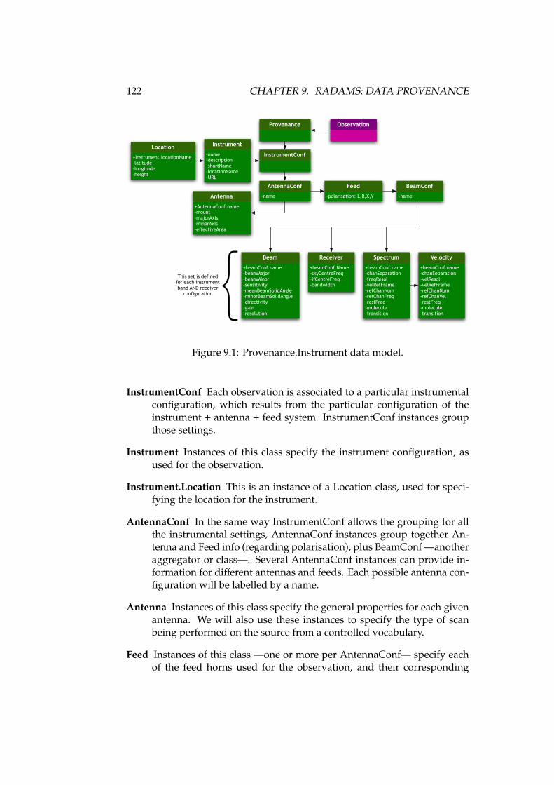
122 CHAPTER 9. RADAMS: DATA PROVENANCE
ObservationProvenance
InstrumentConf
-name
AntennaConf
-polarisation: L,R,X,Y
Feed
-name
BeamConf
+AntennaConf.name-mount-majorAxis-minorAxis-effectiveArea
Antenna
-name-description-shortName-locationName-URL
Instrument
+Instrument.locationName–latitude-longitude-height
Location
+beamConf.name-beamMajor-beamMinor-sensitivity-meanBeamSolidAngle-minorBeamSolidAngle-directivity-gain-resolution
Beam
+beamConf.Name-skyCentreFreq-ifCentreFreq-bandwidth
Receiver
+beamConf.name-chanSeparation-freqResol-velRefFrame-refChanNum-refChanFreq-restFreq-molecule-transition
Spectrum
+beamConf.name-chanSeparation-velResol-velRefFrame-refChanNum-refChanVel-restFreq-molecule-transition
Velocity
This set is defined for each instrument band AND receiver
configuration
Figure 9.1: Provenance.Instrument data model.
InstrumentConf Each observation is associated to a particular instrumentalconfiguration, which results from the particular configuration of theinstrument + antenna + feed system. InstrumentConf instances groupthose settings.
Instrument Instances of this class specify the instrument configuration, asused for the observation.
Instrument.Location This is an instance of a Location class, used for speci-fying the location for the instrument.
AntennaConf In the same way InstrumentConf allows the grouping for allthe instrumental settings, AntennaConf instances group together An-tenna and Feed info (regarding polarisation), plus BeamConf —anotheraggregator or class—. Several AntennaConf instances can provide in-formation for different antennas and feeds. Each possible antenna con-figuration will be labelled by a name.
Antenna Instances of this class specify the general properties for each givenantenna. We will also use these instances to specify the type of scanbeing performed on the source from a controlled vocabulary.
Feed Instances of this class —one or more per AntennaConf— specify eachof the feed horns used for the observation, and their corresponding
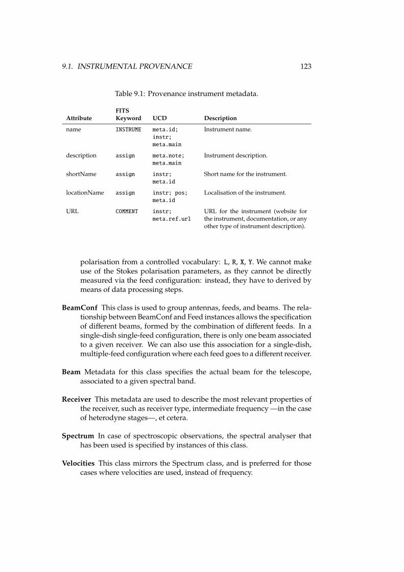
9.1. INSTRUMENTAL PROVENANCE 123
Table 9.1: Provenance instrument metadata.
FITSAttribute Keyword UCD Description
name INSTRUME meta.id;instr;meta.main
Instrument name.
description assign meta.note;meta.main
Instrument description.
shortName assign instr;meta.id
Short name for the instrument.
locationName assign instr; pos;meta.id
Localisation of the instrument.
URL COMMENT instr;meta.ref.url
URL for the instrument (website forthe instrument, documentation, or anyother type of instrument description).
polarisation from a controlled vocabulary: L, R, X, Y. We cannot makeuse of the Stokes polarisation parameters, as they cannot be directlymeasured via the feed configuration: instead, they have to derived bymeans of data processing steps.
BeamConf This class is used to group antennas, feeds, and beams. The rela-tionship between BeamConf and Feed instances allows the specificationof different beams, formed by the combination of different feeds. In asingle-dish single-feed configuration, there is only one beam associatedto a given receiver. We can also use this association for a single-dish,multiple-feed configuration where each feed goes to a different receiver.
Beam Metadata for this class specifies the actual beam for the telescope,associated to a given spectral band.
Receiver This metadata are used to describe the most relevant properties ofthe receiver, such as receiver type, intermediate frequency —in the caseof heterodyne stages—, et cetera.
Spectrum In case of spectroscopic observations, the spectral analyser thathas been used is specified by instances of this class.
Velocities This class mirrors the Spectrum class, and is preferred for thosecases where velocities are used, instead of frequency.
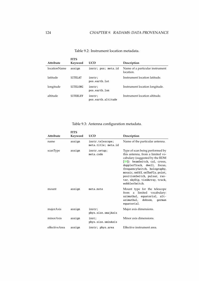
124 CHAPTER 9. RADAMS: DATA PROVENANCE
Table 9.2: Instrument location metadata.
FITSAttribute Keyword UCD Description
locationName assign instr; pos; meta.id Name of a particular instrumentlocation.
latitude SITELAT instr;pos.earth.lat
Instrument location latitude.
longitude SITELONG instr;pos.earth.lon
Instrument location longitude.
altitude SITEELEV instr;pos.earth.altitude
Instrument location altitude.
Table 9.3: Antenna configuration metadata.
FITSAttribute Keyword UCD Description
name assign instr.telescope;meta.title; meta.id
Name of the particular antenna.
scanType assign instr.setup;meta.code
Type of scan being performed bythis antenna, from a limited vo-cabulary (suggested by the RDM[59]): beamSwitch, cal, cross,dopplerTrack, dwell, focus,frequencySwitch, holography,mosaic, onOff, onTheFly, point,positionSwitch, pulsar, ras-ter, skyDip, tiedArray, track,wobblerSwitch.
mount assign meta.note Mount type for the telescopefrom a limited vocabulary:azimuthal, equatorial, alt-azimuthal, dobson, germanequatorial.
majorAxis assign instr;phys.size.smajAxis
Major axis dimensions.
minorAxis assign inst;phys.size.sminAxis
Minor axis dimensions.
effectiveArea assign instr; phys.area Effective instrument area.
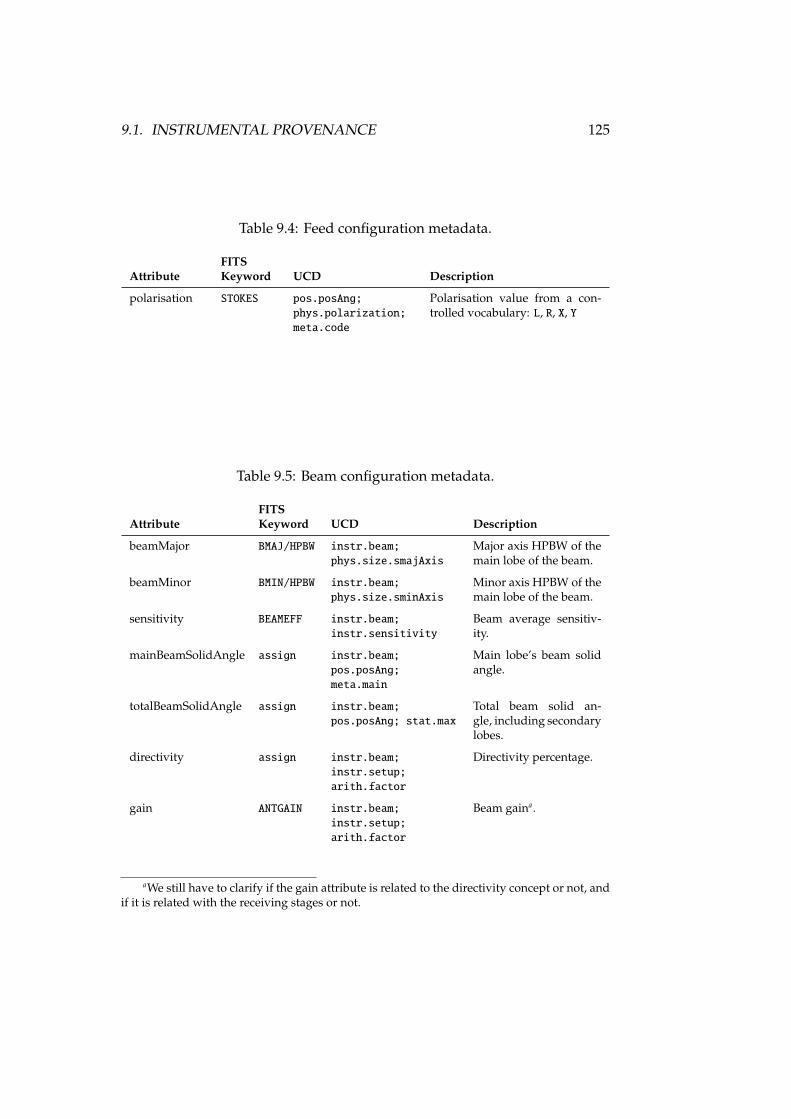
9.1. INSTRUMENTAL PROVENANCE 125
Table 9.4: Feed configuration metadata.
FITSAttribute Keyword UCD Description
polarisation STOKES pos.posAng;phys.polarization;meta.code
Polarisation value from a con-trolled vocabulary: L, R, X, Y
Table 9.5: Beam configuration metadata.
FITSAttribute Keyword UCD Description
beamMajor BMAJ/HPBW instr.beam;phys.size.smajAxis
Major axis HPBW of themain lobe of the beam.
beamMinor BMIN/HPBW instr.beam;phys.size.sminAxis
Minor axis HPBW of themain lobe of the beam.
sensitivity BEAMEFF instr.beam;instr.sensitivity
Beam average sensitiv-ity.
mainBeamSolidAngle assign instr.beam;pos.posAng;meta.main
Main lobe’s beam solidangle.
totalBeamSolidAngle assign instr.beam;pos.posAng; stat.max
Total beam solid an-gle, including secondarylobes.
directivity assign instr.beam;instr.setup;arith.factor
Directivity percentage.
gain ANTGAIN instr.beam;instr.setup;arith.factor
Beam gaina.
aWe still have to clarify if the gain attribute is related to the directivity concept or not, andif it is related with the receiving stages or not.

126 CHAPTER 9. RADAMS: DATA PROVENANCE
Table 9.6: Receiver metadata.
FITSAttribute Keyword UCD Description
type BACKEND instr.setup;meta.note
Receiver type (HEMT, Bolometer, SIS,et cetera).
skyCentreFreq assign src; em.radio;em.freq
Antenna tuning frequency.
IFCentreFreq assign instr.setup;em.freq
Heterodyne receiver intermediate fre-quency (or list of frequencies).
bandwidth BANDWID instr.bandwidth Filter-bank total bandwidth.
Table 9.7: Spectrum metadata. It might be necessary to change the MOLECULEand TRANSITI keywords by LINE, for better CLASS compatibility.
FITSAttribute Keyword UCD Description
numChannels NAXISn spect; em.freq;meta.number
Number of spectral channels.
chanSeparationa assign spect; em.freq Mean channel separation (infrequency units), or channelfrequency separation array.
freqResolution FREQRES spect.resolution;em.freq
Frequency resolution.
refChanNum assign spect; em.freq;meta.number;meta.ref
Spectral reference channel.
refChanFreq OBSFREQ spect; em.freq;meta.code; meta.ref
Spectral reference frequency(observed frequency).
restFreq FREQn orRESTFREQ
spect.line; em.freq Observed spectral line rest fre-quency.
molecule MOLECULEb spect; phys.mol;meta.id
Molecule name.
transition TRANSITIc spect;phys.atmol.transition;meta.id
Transition.
aThere is a certain redundancy between the Provenance.Spectrum.chanSeparation at-tribute and the Coverage.Spectral.Resolution attributes.
bIt might be necessary to change the MOLECULE keyword by LINE, for better CLASS com-patibility.
cIt might be necessary to change the TRANSITI keyword by LINE, for better CLASS com-patibility.
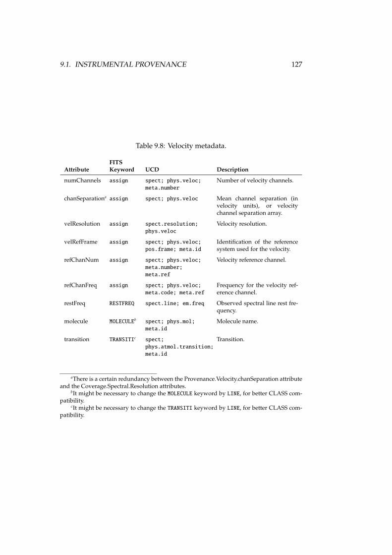
9.1. INSTRUMENTAL PROVENANCE 127
Table 9.8: Velocity metadata.
FITSAttribute Keyword UCD Description
numChannels assign spect; phys.veloc;meta.number
Number of velocity channels.
chanSeparationa assign spect; phys.veloc Mean channel separation (invelocity units), or velocitychannel separation array.
velResolution assign spect.resolution;phys.veloc
Velocity resolution.
velRefFrame assign spect; phys.veloc;pos.frame; meta.id
Identification of the referencesystem used for the velocity.
refChanNum assign spect; phys.veloc;meta.number;meta.ref
Velocity reference channel.
refChanFreq assign spect; phys.veloc;meta.code; meta.ref
Frequency for the velocity ref-erence channel.
restFreq RESTFREQ spect.line; em.freq Observed spectral line rest fre-quency.
molecule MOLECULEb spect; phys.mol;meta.id
Molecule name.
transition TRANSITIc spect;phys.atmol.transition;meta.id
Transition.
aThere is a certain redundancy between the Provenance.Velocity.chanSeparation attributeand the Coverage.Spectral.Resolution attributes.
bIt might be necessary to change the MOLECULE keyword by LINE, for better CLASS com-patibility.
cIt might be necessary to change the TRANSITI keyword by LINE, for better CLASS com-patibility.
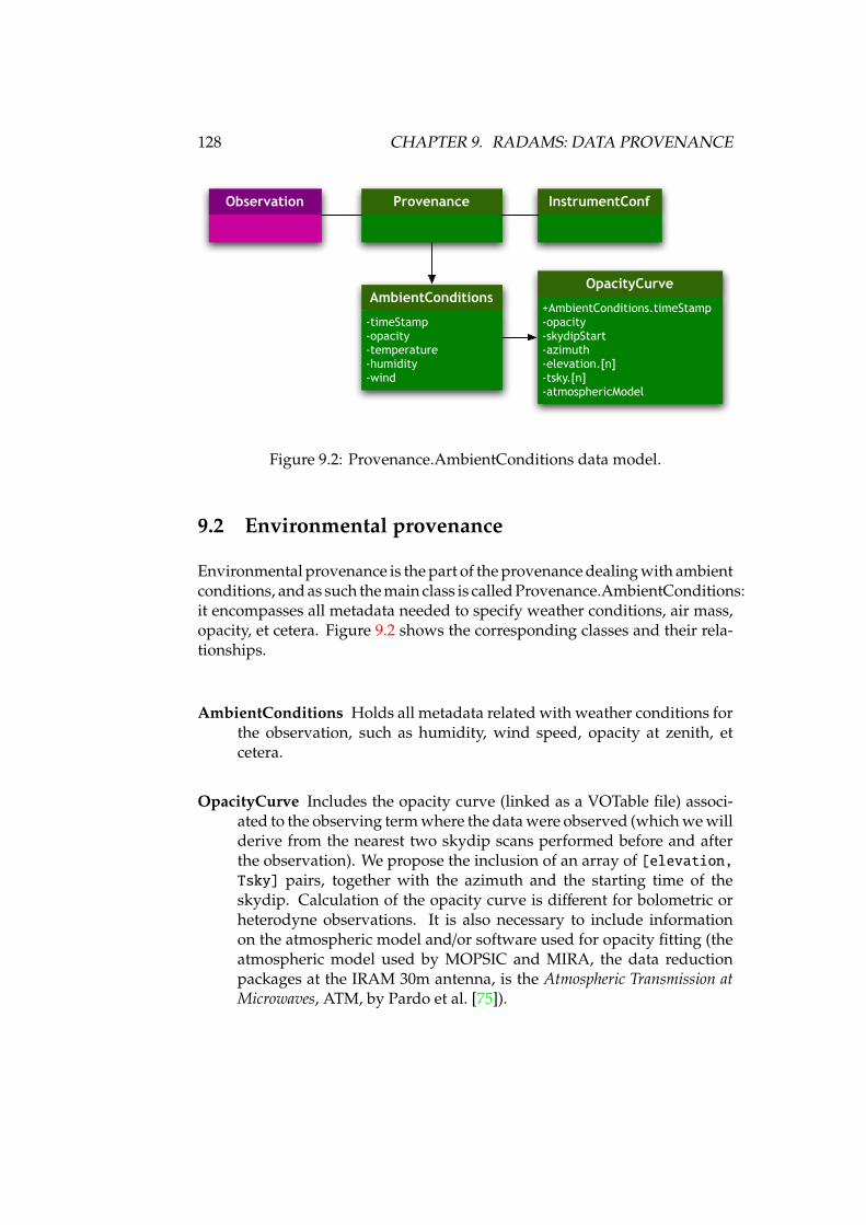
128 CHAPTER 9. RADAMS: DATA PROVENANCE
Observation Provenance InstrumentConf
-timeStamp-opacity-temperature-humidity-wind
AmbientConditions+AmbientConditions.timeStamp-opacity-skydipStart-azimuth-elevation.[n]-tsky.[n]-atmosphericModel
OpacityCurve
Figure 9.2: Provenance.AmbientConditions data model.
9.2 Environmental provenance
Environmental provenance is the part of the provenance dealing with ambientconditions, and as such the main class is called Provenance.AmbientConditions:it encompasses all metadata needed to specify weather conditions, air mass,opacity, et cetera. Figure 9.2 shows the corresponding classes and their rela-tionships.
AmbientConditions Holds all metadata related with weather conditions forthe observation, such as humidity, wind speed, opacity at zenith, etcetera.
OpacityCurve Includes the opacity curve (linked as a VOTable file) associ-ated to the observing term where the data were observed (which we willderive from the nearest two skydip scans performed before and afterthe observation). We propose the inclusion of an array of [elevation,Tsky] pairs, together with the azimuth and the starting time of theskydip. Calculation of the opacity curve is different for bolometric orheterodyne observations. It is also necessary to include informationon the atmospheric model and/or software used for opacity fitting (theatmospheric model used by MOPSIC and MIRA, the data reductionpackages at the IRAM 30m antenna, is the Atmospheric Transmission atMicrowaves, ATM, by Pardo et al. [75]).
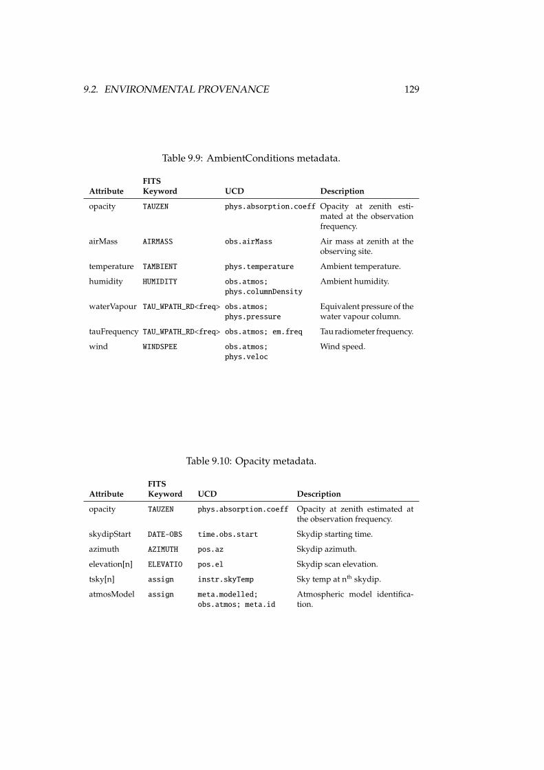
9.2. ENVIRONMENTAL PROVENANCE 129
Table 9.9: AmbientConditions metadata.
FITSAttribute Keyword UCD Description
opacity TAUZEN phys.absorption.coeff Opacity at zenith esti-mated at the observationfrequency.
airMass AIRMASS obs.airMass Air mass at zenith at theobserving site.
temperature TAMBIENT phys.temperature Ambient temperature.
humidity HUMIDITY obs.atmos;phys.columnDensity
Ambient humidity.
waterVapour TAU_WPATH_RD<freq> obs.atmos;phys.pressure
Equivalent pressure of thewater vapour column.
tauFrequency TAU_WPATH_RD<freq> obs.atmos; em.freq Tau radiometer frequency.
wind WINDSPEE obs.atmos;phys.veloc
Wind speed.
Table 9.10: Opacity metadata.
FITSAttribute Keyword UCD Description
opacity TAUZEN phys.absorption.coeff Opacity at zenith estimated atthe observation frequency.
skydipStart DATE-OBS time.obs.start Skydip starting time.
azimuth AZIMUTH pos.az Skydip azimuth.
elevation[n] ELEVATIO pos.el Skydip scan elevation.
tsky[n] assign instr.skyTemp Sky temp at nth skydip.
atmosModel assign meta.modelled;obs.atmos; meta.id
Atmospheric model identifica-tion.
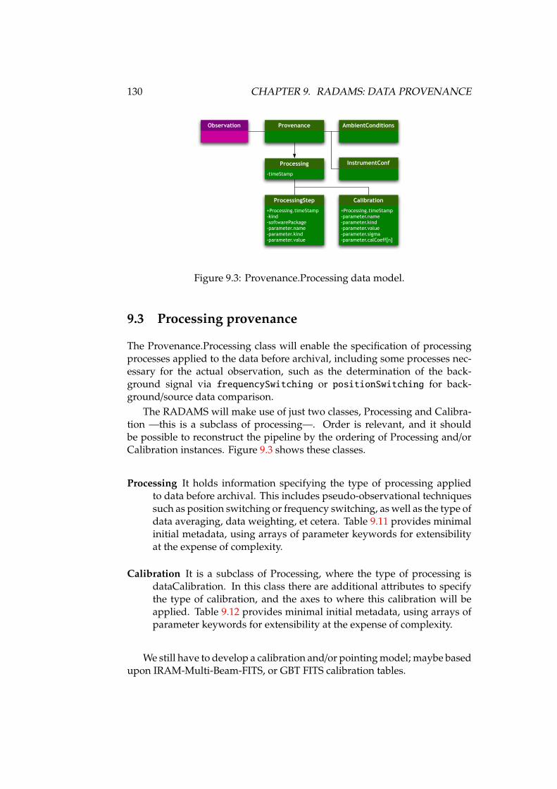
130 CHAPTER 9. RADAMS: DATA PROVENANCE
InstrumentConf
-timeStamp
Processing
Observation Provenance AmbientConditions
+Processing.timeStamp-parameter.name-parameter.kind-parameter.value-parameter.sigma-parameter.calCoeff[n]
Calibration
+Processing.timeStamp-kind-softwarePackage-parameter.name-parameter.kind-parameter.value
ProcessingStep
Figure 9.3: Provenance.Processing data model.
9.3 Processing provenance
The Provenance.Processing class will enable the specification of processingprocesses applied to the data before archival, including some processes nec-essary for the actual observation, such as the determination of the back-ground signal via frequencySwitching or positionSwitching for back-ground/source data comparison.
The RADAMS will make use of just two classes, Processing and Calibra-tion —this is a subclass of processing—. Order is relevant, and it shouldbe possible to reconstruct the pipeline by the ordering of Processing and/orCalibration instances. Figure 9.3 shows these classes.
Processing It holds information specifying the type of processing appliedto data before archival. This includes pseudo-observational techniquessuch as position switching or frequency switching, as well as the type ofdata averaging, data weighting, et cetera. Table 9.11 provides minimalinitial metadata, using arrays of parameter keywords for extensibilityat the expense of complexity.
Calibration It is a subclass of Processing, where the type of processing isdataCalibration. In this class there are additional attributes to specifythe type of calibration, and the axes to where this calibration will beapplied. Table 9.12 provides minimal initial metadata, using arrays ofparameter keywords for extensibility at the expense of complexity.
We still have to develop a calibration and/or pointing model; maybe basedupon IRAM-Multi-Beam-FITS, or GBT FITS calibration tables.
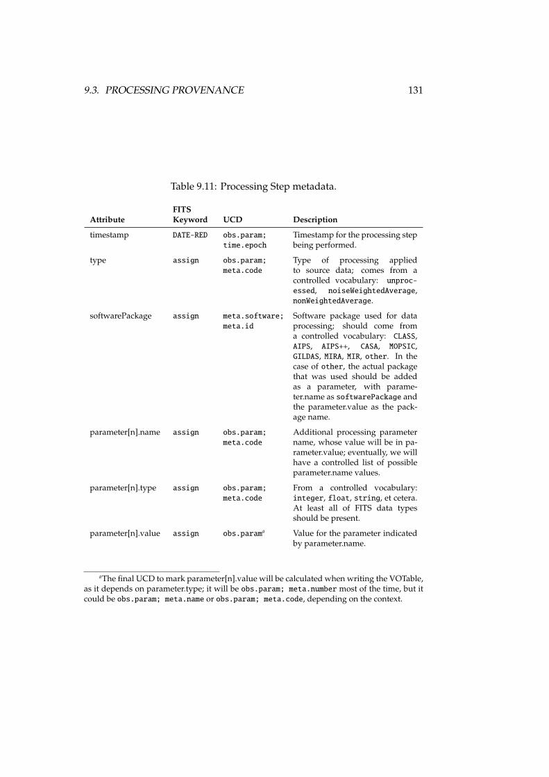
9.3. PROCESSING PROVENANCE 131
Table 9.11: Processing Step metadata.
FITSAttribute Keyword UCD Description
timestamp DATE-RED obs.param;time.epoch
Timestamp for the processing stepbeing performed.
type assign obs.param;meta.code
Type of processing appliedto source data; comes from acontrolled vocabulary: unproc-essed, noiseWeightedAverage,nonWeightedAverage.
softwarePackage assign meta.software;meta.id
Software package used for dataprocessing; should come froma controlled vocabulary: CLASS,AIPS, AIPS++, CASA, MOPSIC,GILDAS, MIRA, MIR, other. In thecase of other, the actual packagethat was used should be addedas a parameter, with parame-ter.name as softwarePackage andthe parameter.value as the pack-age name.
parameter[n].name assign obs.param;meta.code
Additional processing parametername, whose value will be in pa-rameter.value; eventually, we willhave a controlled list of possibleparameter.name values.
parameter[n].type assign obs.param;meta.code
From a controlled vocabulary:integer, float, string, et cetera.At least all of FITS data typesshould be present.
parameter[n].value assign obs.parama Value for the parameter indicatedby parameter.name.
aThe final UCD to mark parameter[n].value will be calculated when writing the VOTable,as it depends on parameter.type; it will be obs.param; meta.number most of the time, but itcould be obs.param; meta.name or obs.param; meta.code, depending on the context.
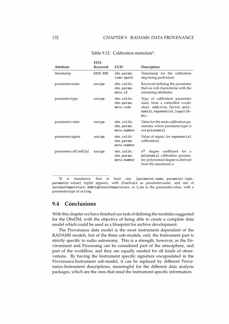
132 CHAPTER 9. RADAMS: DATA PROVENANCE
Table 9.12: Calibration metadataa.
FITSAttribute Keyword UCD Description
timestamp DATE-RED obs.param;time.epoch
Timestamp for the calibrationstep being performed.
parameter.name assign obs.calib;obs.param;meta.id
Keyword defining the parameterthat we will characterise with theremaining attributes.
parameter.type assign obs.calib;obs.param;meta.code
Type of calibration parameterused, from a controlled vocab-ulary: additive, factor, poly-nomial, exponential, logarith-mic.
parameter.value assign obs.calib;obs.param;meta.number
Value for the main calibration pa-rameter, where parameter.type isnot polynomial.
parameter.sigma assign obs.calib;obs.param;meta.number
Value of sigma, for exponentialcalibrations.
parameter.calCoeff.[n] assign obs.calib;obs.param;meta.number
nth degree coefficient for apolynomial calibration parame-ter; polynomial degree is derivedfrom the maximum n.
aIt is mandatory that at least one [parameter.name, parameter.type,parameter.value] triplet appears, with fluxScale as parameter.name, and one ofantennaTemperature, mbBrightnessTemperature, or S_nu as the parameter.value, with aparameter.type of string.
9.4 Conclusions
With this chapter we have finished our task of defining the modules suggestedfor the ObsDM, with the objective of being able to create a complete datamodel which could be used as a blueprint for archive development.
The Provenance data model is the most instrument dependant of theRADAMS models, but of the three sub-models, only the Instrument part isstrictly specific to radio astronomy. This is a strength, however, as the En-vironment and Processing can be considered part of the atmosphere, andpart of the workflow, and they are equally needed for all kinds of obser-vations. By having the Instrument specific signature encapsulated in theProvenance.Instrument sub-model, it can be replaced by different Prove-nance.Instrument descriptions, meaningful for the different data analysispackages, which are the ones that need the instrument-specific information.
Part III
Bringing legacy tools to the VO
133

Chapter 10
Legacy astronomical packagesand the VO
legacynoun• a thing handed down by a predecessor: the
legacy of centuries of neglect.legacyadjective (computing)• Denoting software or hardware that has been
superseded but is difficult to replace becauseof its wide use.
The New Oxford American Dictionary, 2nd Edition
The physical properties we can ascertain from remote astronomical objectsare the result of careful computations on observed datasets, which tend tobe observatory, telescope, instrument, and even observing mode specific.Such computations include background noise estimations, electron counts toincident flux conversions, instrument signal removal, et cetera.
Many different software packages have been developed for performingthose operations (which are commonly known as data reduction), and obtain-ing science-ready data products (i.e., images which have been flux calibrated,given precise astrometry, et cetera), and analysing them to get additionalphysical information. For instance, once a spectrum has been calibrated onthe local standard of rest of the source, the width of an emission line can bedirectly correlated to an expansion or contraction velocity of the observedobject.
The investment in man-years on these applications is enormous, andeven when they have been developed using techniques available many yearsago, and can be considered superseded, the recreation of all the algorithmsin modern languages, or on more modern GUI framework foundations is
135
136 CHAPTER 10. LEGACY ASTRONOMICAL PACKAGES AND THE VO
prohibitive, due to the extensive development and testing that would beneeded for such a replacement.
Examples of 30-year old software packages still in heavy use includeAIPS1, a radio astronomical imaging package from the late seventies orig-inally written in FORTRAN IV; or GIPSY2, a 3D data analysis package forobtaining kinematic properties, whose development started in the early sev-enties, and is also written in FORTRAN.
But the goal set for the VO is to be, in the future, the entire framework forastronomical and astrophysical computing, both for its development and itsexecution, becoming completely transparent to astronomical users.
We cannot expect, then, astronomers to embrace the VO without thetools they are accustomed to, and we cannot recreate all the existing legacyapplications. We must, therefore, find a way to bring these legacy applicationsinto the VO, and that is the scope of this chapter: How to bring legacy applicationsinto the VO environment.
10.1 VO-enabling applications
We must start by answering the question What is a VO-enabled application?From the many VO standards and protocols issued by the IVOA3, which andhow many of them have to be implemented for us to consider an applicationis VO-enabled?
We will understand that a VO-enabled application is a software packagewhich:
1. Can read and/or write data in VOTable (and possibly FITS) format.
2. Can query the VO Registry in order to find VO services or data resources,at least of one particular kind.
3. Can call a subset of VO-registered services for at least one of IVOA dataaccess protocols4.
A somehow orthogonal capability is that of being able to communicatewith other VO applications running in the same machine, via the soon to beapproved Simple Application Messaging Protocol (SAMP) [76].
However, an application which can use SAMP to communicate with otherscan in fact make use of their capabilities, and retrieve the data processed fromothers. Conversely, the processed results can be mixed with those of anyother application.
We can, then, consider that a VO application is just one which:
1http://www.aips.nrao.edu/2http://www.astro.rug.nl/~gipsy/3http://ivoa.net/Documents/4ConeSearch, Simple Image Access, or Simple Spectra Access. See appendix D.
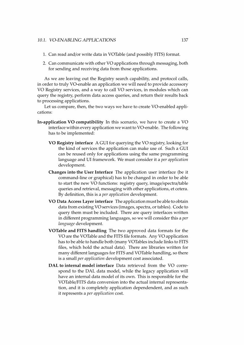
10.1. VO-ENABLING APPLICATIONS 137
1. Can read and/or write data in VOTable (and possibly FITS) format.
2. Can communicate with other VO applications through messaging, bothfor sending and receiving data from those applications.
As we are leaving out the Registry search capability, and protocol calls,in order to truly VO-enable an application we will need to provide accessoryVO Registry services, and a way to call VO services, in modules which canquery the registry, perform data access queries, and return their results backto processing applications.
Let us compare, then, the two ways we have to create VO-enabled appli-cations:
In-application VO compatibility In this scenario, we have to create a VOinterface within every application we want to VO-enable. The followinghas to be implemented:
VO Registry interface A GUI for querying the VO registry, looking forthe kind of services the application can make use of. Such a GUIcan be reused only for applications using the same programminglanguage and UI framework. We must consider it a per applicationdevelopment.
Changes into the User Interface The application user interface (be itcommand-line or graphical) has to be changed in order to be ableto start the new VO functions: registry query, image/spectra/tablequeries and retrieval, messaging with other applications, et cetera.By definition, this is a per application development.
VO Data Access Layer interface The application must be able to obtaindata from existing VO services (images, spectra, or tables). Code toquery them must be included. There are query interfaces writtenin different programming languages, so we will consider this a perlanguage development.
VOTable and FITS handling The two approved data formats for theVO are the VOTable and the FITS file formats. Any VO applicationhas to be able to handle both (many VOTables include links to FITSfiles, which hold the actual data). There are libraries written formany different languages for FITS and VOTable handling, so thereis a small per application development cost associated.
DAL to internal model interface Data retrieved from the VO corre-spond to the DAL data model, while the legacy application willhave an internal data model of its own. This is responsible for theVOTable/FITS data conversion into the actual internal representa-tion, and it is completely application dependendent, and as suchit represents a per application cost.
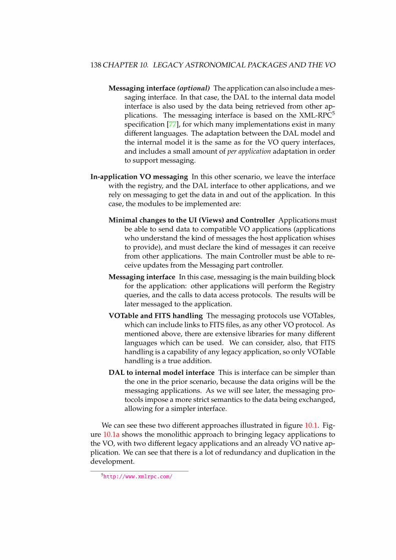
138 CHAPTER 10. LEGACY ASTRONOMICAL PACKAGES AND THE VO
Messaging interface (optional) The application can also include a mes-saging interface. In that case, the DAL to the internal data modelinterface is also used by the data being retrieved from other ap-plications. The messaging interface is based on the XML-RPC5
specification [77], for which many implementations exist in manydifferent languages. The adaptation between the DAL model andthe internal model it is the same as for the VO query interfaces,and includes a small amount of per application adaptation in orderto support messaging.
In-application VO messaging In this other scenario, we leave the interfacewith the registry, and the DAL interface to other applications, and werely on messaging to get the data in and out of the application. In thiscase, the modules to be implemented are:
Minimal changes to the UI (Views) and Controller Applications mustbe able to send data to compatible VO applications (applicationswho understand the kind of messages the host application whisesto provide), and must declare the kind of messages it can receivefrom other applications. The main Controller must be able to re-ceive updates from the Messaging part controller.
Messaging interface In this case, messaging is the main building blockfor the application: other applications will perform the Registryqueries, and the calls to data access protocols. The results will belater messaged to the application.
VOTable and FITS handling The messaging protocols use VOTables,which can include links to FITS files, as any other VO protocol. Asmentioned above, there are extensive libraries for many differentlanguages which can be used. We can consider, also, that FITShandling is a capability of any legacy application, so only VOTablehandling is a true addition.
DAL to internal model interface This is interface can be simpler thanthe one in the prior scenario, because the data origins will be themessaging applications. As we will see later, the messaging pro-tocols impose a more strict semantics to the data being exchanged,allowing for a simpler interface.
We can see these two different approaches illustrated in figure 10.1. Fig-ure 10.1a shows the monolithic approach to bringing legacy applications tothe VO, with two different legacy applications and an already VO native ap-plication. We can see that there is a lot of redundancy and duplication in thedevelopment.
5http://www.xmlrpc.com/
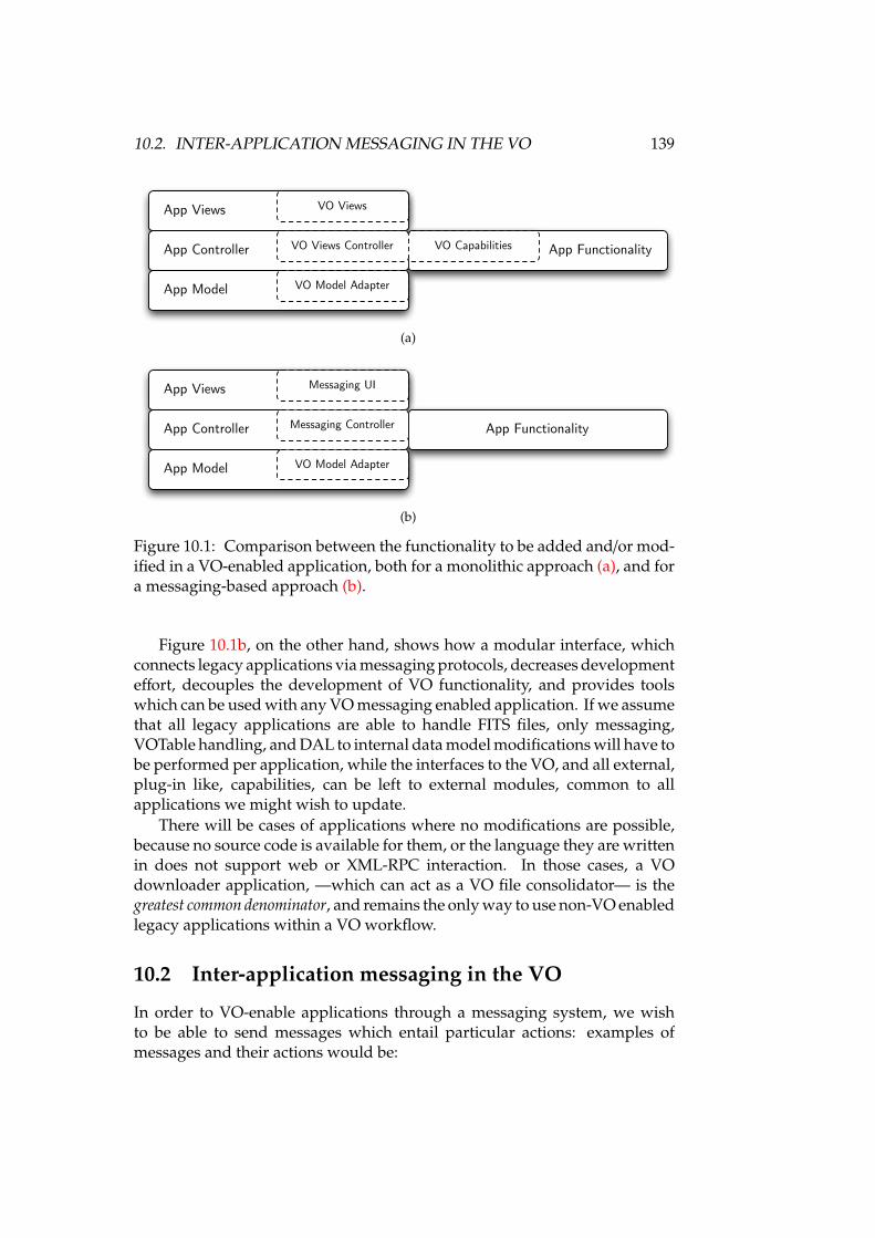
10.2. INTER-APPLICATION MESSAGING IN THE VO 139
App Views
App Controller
App Model
VO Views
VO Views Controller
VO Model Adapter
App FunctionalityVO Capabilities
(a)
App Views
App Controller
App Model
Messaging UI
Messaging Controller
VO Model Adapter
App Functionality
(b)
Figure 10.1: Comparison between the functionality to be added and/or mod-ified in a VO-enabled application, both for a monolithic approach (a), and fora messaging-based approach (b).
Figure 10.1b, on the other hand, shows how a modular interface, whichconnects legacy applications via messaging protocols, decreases developmenteffort, decouples the development of VO functionality, and provides toolswhich can be used with any VO messaging enabled application. If we assumethat all legacy applications are able to handle FITS files, only messaging,VOTable handling, and DAL to internal data model modifications will have tobe performed per application, while the interfaces to the VO, and all external,plug-in like, capabilities, can be left to external modules, common to allapplications we might wish to update.
There will be cases of applications where no modifications are possible,because no source code is available for them, or the language they are writtenin does not support web or XML-RPC interaction. In those cases, a VOdownloader application, —which can act as a VO file consolidator— is thegreatest common denominator, and remains the only way to use non-VO enabledlegacy applications within a VO workflow.
10.2 Inter-application messaging in the VO
In order to VO-enable applications through a messaging system, we wishto be able to send messages which entail particular actions: examples ofmessages and their actions would be:
140 CHAPTER 10. LEGACY ASTRONOMICAL PACKAGES AND THE VO
• Issuing a data load message, and having data loaded on the remoteapplication.
• Issuing a highlight data message, and have the data highlighted on theremote application.
Without taking into account the nature of the data (in the VO, data ispassed by means of VOTables, which might contain data, or link to data), itis clear that there might be several receivers for messages of this nature, so amechanism for registering potential receivers of messages is needed. If thenumber of possible messages is moderate to large, an application would alsoneed to declare the kind of messages it can deal with.
We can see that a possible solution to this are publish-subscribe mecha-nisms, where several parties can act as information publishers, and several(possibly different) parties act as information subscribers. A thorough reviewof publish-subscribe mechanisms has been performed by Eugster et al. [78].
The first messaging mechanism within the VO was an experiment by theVOTech project6, and was the PLatform for AStronomical Tool InterConnec-tion7 (PLASTIC) [79], a client-side messaging protocol.
PLASTIC was based on XML-RPC messaging between client applicationsand a central hub which had to start before the applications could connectto it. Applications would register the messages they support, and wouldprovide handler functions for incoming messages (callbacks).
The number of defined messages was not very large, and by being imple-mented on top of XML-RPC it was easily ported to different languages andplatforms. In fact, in spite of never being an IVOA standard, the number ofapplications supporting PLASTIC was very high, as the cost of implementingPLASTIC capabilities was very low.
However, PLASTIC sported a number of shortcomings:
Hard-coded message types and parameters The messages types were hard-coded in the protocol, making messages fixed, and not extensible. Smallmodifications to an existing message were not possible, as all parame-ters were fixed by the message definition.
Non-uniform messages Each message had a number of parameters that de-pended entirely on the message type, without any governing rule.
Java-based typing Data types were based on Java data types, instead ofrelying on platform-independent data type definitions.
6In turn, inspired by the XPA (uniX Public Access, http://hea-www.harvard.edu/RD/xpa/intro.html) protocol used for communication between tools written for the X11 win-dowing system, or Tcl/Tk, or Perl packages, such as IRAF, or the SAOImage DS9 FITS viewer.IRAF, for instance, can use DS9 as its imaging package thanks to XPA.
7http://plastic.sourceforge.net/
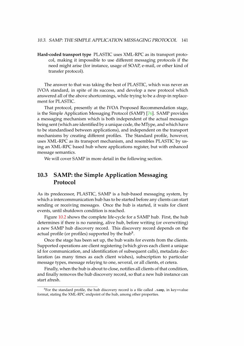
10.3. SAMP: THE SIMPLE APPLICATION MESSAGING PROTOCOL 141
Hard-coded transport type PLASTIC uses XML-RPC as its transport proto-col, making it impossible to use different messaging protocols if theneed might arise (for instance, usage of SOAP, e-mail, or other kind oftransfer protocol).
The answer to that was taking the best of PLASTIC, which was never anIVOA standard, in spite of its success, and develop a new protocol whichanswered all of the above shortcomings, while trying to be a drop-in replace-ment for PLASTIC.
That protocol, presently at the IVOA Proposed Recommendation stage,is the Simple Application Messaging Protocol (SAMP) [76]. SAMP providesa messaging mechanism which is both independent of the actual messagesbeing sent (which are identified by a unique code, the MType, and which haveto be standardised between applications), and independent on the transportmechanisms by creating different profiles. The Standard profile, however,uses XML-RPC as its transport mechanism, and resembles PLASTIC by us-ing an XML-RPC based hub where applications register, but with enhancedmessage semantics.
We will cover SAMP in more detail in the following section.
10.3 SAMP: the Simple Application MessagingProtocol
As its predecessor, PLASTIC, SAMP is a hub-based messaging system, bywhich a intercommunication hub has to be started before any clients can startsending or receiving messages. Once the hub is started, it waits for clientevents, until shutdown condition is reached.
Figure 10.2 shows the complete life-cycle for a SAMP hub. First, the hubdetermines if there is no running, alive hub, before writing (or overwriting)a new SAMP hub discovery record. This discovery record depends on theactual profile (or profiles) supported by the hub8.
Once the stage has been set up, the hub waits for events from the clients.Supported operations are client registering (which gives each client a uniqueid for communication, and identification of subsequent calls), metadata dec-laration (as many times as each client wishes), subscription to particularmessage types, message relaying to one, several, or all clients, et cetera.
Finally, when the hub is about to close, notifies all clients of that condition,and finally removes the hub discovery record, so that a new hub instance canstart afresh.
8For the standard profile, the hub discovery record is a file called .samp, in key=valueformat, stating the XML-RPC endpoint of the hub, among other properties.

142 CHAPTER 10. LEGACY ASTRONOMICAL PACKAGES AND THE VO
Start
Is there a running hub?
Is the hub alive?
Create/Overwrite discovery record
Wait for events
Client registration
Client metadata (re)declara
tion
Client subscription
change
Hub about to
shutdown
End
Message received for
relaying
Client unregisters
Client determined
dead
no
no
yes
yes
1
2
3 4 5 6 7 8
Figure 10.2: Life-cycle of a SAMP hub. Once determined there is no running,alive hub, the discovery record is created, and the hub waits for the differentevents it supports, until shutdown. The numbers on the black circles will beused to refer to particular steps throughout the text.
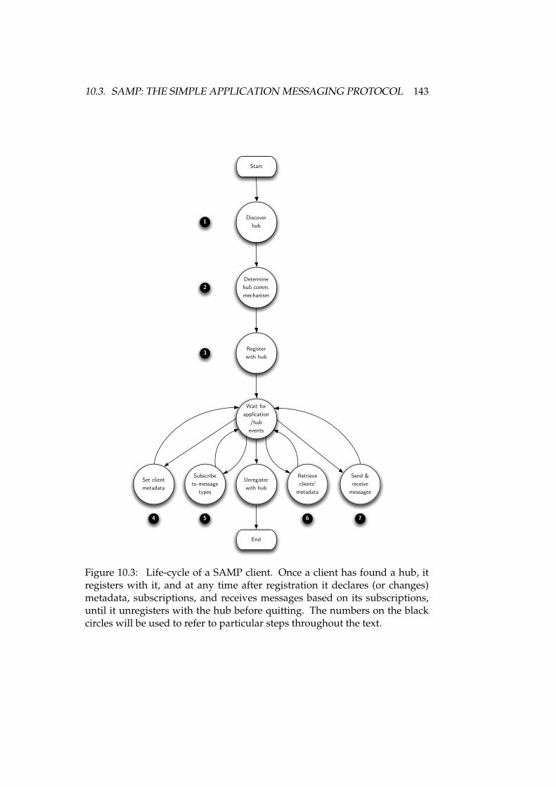
10.3. SAMP: THE SIMPLE APPLICATION MESSAGING PROTOCOL 143
Discover hub
Start
Determine hub comm. mechanism
Register with hub
Wait for application
/hub events
Set client metadata
Subscribe to message
types
Unregister with hub
End
Retrieve clients'
metadata
Send & receive
messages
1
2
3
4 5 6 7
Figure 10.3: Life-cycle of a SAMP client. Once a client has found a hub, itregisters with it, and at any time after registration it declares (or changes)metadata, subscriptions, and receives messages based on its subscriptions,until it unregisters with the hub before quitting. The numbers on the blackcircles will be used to refer to particular steps throughout the text.
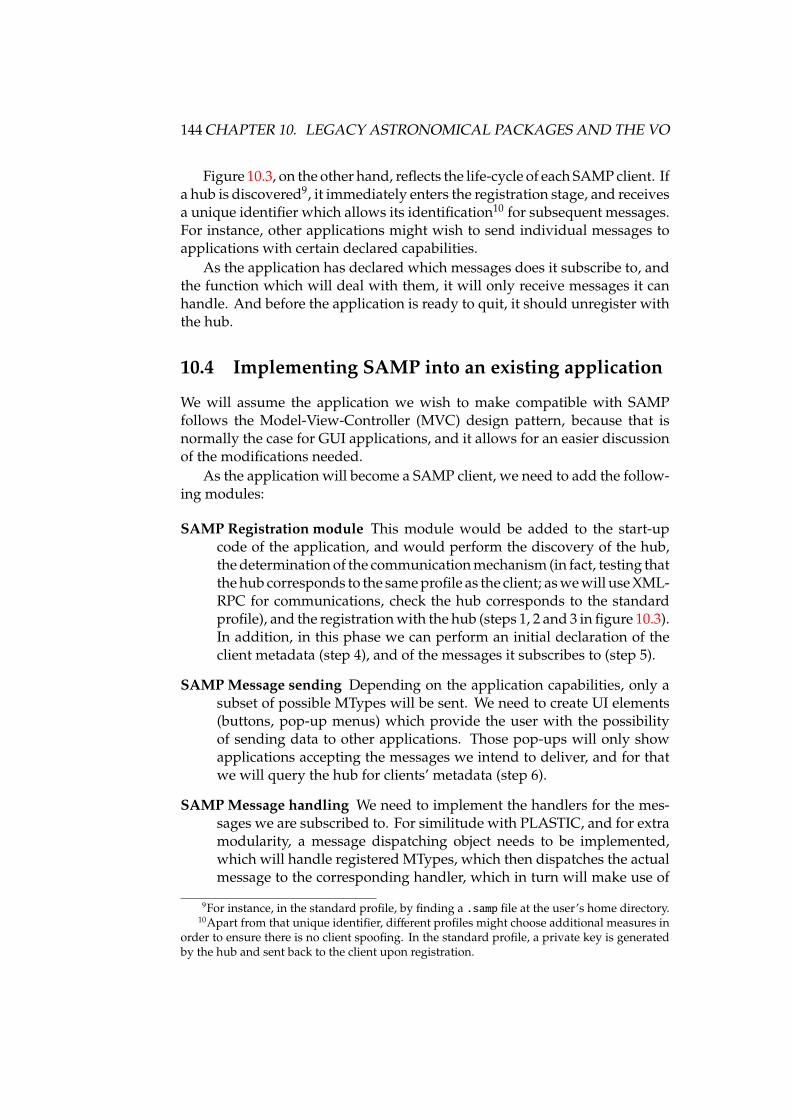
144 CHAPTER 10. LEGACY ASTRONOMICAL PACKAGES AND THE VO
Figure 10.3, on the other hand, reflects the life-cycle of each SAMP client. Ifa hub is discovered9, it immediately enters the registration stage, and receivesa unique identifier which allows its identification10 for subsequent messages.For instance, other applications might wish to send individual messages toapplications with certain declared capabilities.
As the application has declared which messages does it subscribe to, andthe function which will deal with them, it will only receive messages it canhandle. And before the application is ready to quit, it should unregister withthe hub.
10.4 Implementing SAMP into an existing application
We will assume the application we wish to make compatible with SAMPfollows the Model-View-Controller (MVC) design pattern, because that isnormally the case for GUI applications, and it allows for an easier discussionof the modifications needed.
As the application will become a SAMP client, we need to add the follow-ing modules:
SAMP Registration module This module would be added to the start-upcode of the application, and would perform the discovery of the hub,the determination of the communication mechanism (in fact, testing thatthe hub corresponds to the same profile as the client; as we will use XML-RPC for communications, check the hub corresponds to the standardprofile), and the registration with the hub (steps 1, 2 and 3 in figure 10.3).In addition, in this phase we can perform an initial declaration of theclient metadata (step 4), and of the messages it subscribes to (step 5).
SAMP Message sending Depending on the application capabilities, only asubset of possible MTypes will be sent. We need to create UI elements(buttons, pop-up menus) which provide the user with the possibilityof sending data to other applications. Those pop-ups will only showapplications accepting the messages we intend to deliver, and for thatwe will query the hub for clients’ metadata (step 6).
SAMP Message handling We need to implement the handlers for the mes-sages we are subscribed to. For similitude with PLASTIC, and for extramodularity, a message dispatching object needs to be implemented,which will handle registered MTypes, which then dispatches the actualmessage to the corresponding handler, which in turn will make use of
9For instance, in the standard profile, by finding a .samp file at the user’s home directory.10Apart from that unique identifier, different profiles might choose additional measures in
order to ensure there is no client spoofing. In the standard profile, a private key is generatedby the hub and sent back to the client upon registration.
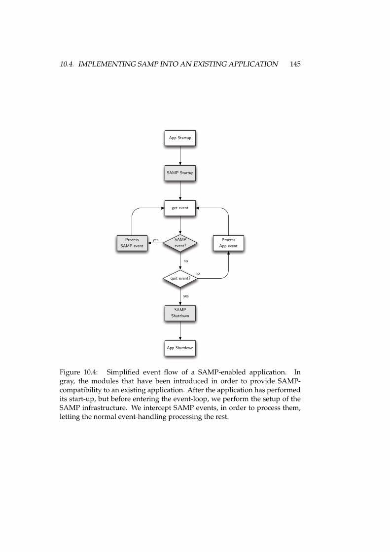
10.4. IMPLEMENTING SAMP INTO AN EXISTING APPLICATION 145
App Startup
SAMP Startup
get event
SAMP event?
quit event?
SAMP Shutdown
App Shutdown
Process SAMP event
Process App event
yes
yes
no
no
Figure 10.4: Simplified event flow of a SAMP-enabled application. Ingray, the modules that have been introduced in order to provide SAMP-compatibility to an existing application. After the application has performedits start-up, but before entering the event-loop, we perform the setup of theSAMP infrastructure. We intercept SAMP events, in order to process them,letting the normal event-handling processing the rest.
146 CHAPTER 10. LEGACY ASTRONOMICAL PACKAGES AND THE VO
existing application functionality to either display or manipulate thereceived message. This corresponds to handling of step 7.
In addition, some small modifications to the main view controller willhave to performed, so that incoming messages with data can be dealt withas if an open file event had been issued. If the application is well factored,changes to the controller can be inexistent.
The changes needed to the application flow are shown in figure 10.4. Themain simplification is the Process SAMP event box, which apart from possi-bly reissuing application-specific events in order to complete event processing(i.e., for finishing a table load message with an actual data load, in the internaldata format of the application; if the application load messages handle FITSfiles, the changes would be minor).
10.5 Benefits of a SAMP-based API
By implementing SAMP on an existing astronomical application, we havegiven it the opportunity to interact with other VO applications, and leavedata selection in the VO to external applications.
However, given that SAMP, as a publish, subscribe, and messaging facilityallows any kind of messages, by defining ad-hoc MTypes we can create newfunctionality that responds in particular ways to given MTypes and theirparameters. This way, we can create a complete Application ProgrammingInterface, in which instead of providing actual, byte-compiled functions, thefunctionality is provided via SAMP messages calls and responses.
Of course, given that the standard profile for SAMP uses XML-RPC, wecould have created such an API as XML-RPC instances. However, bringingthe API to SAMP has the following advantages, both over an XML-RPC APIor pure binary API:
Modularity The building blocks for a SAMP-based API are the supportedMTypes, or families of closely related MTypes. But in any case, anymodule can provide support for one or more MTypes. It brings theclassical do one thing well motto typical from UNIX tools to the VO11.
Discoverability of services In order to be able to receive the MType messageswhich conform the API, functional modules need to register with theSAMP hub. Any application can query the hub, and request a list of theapplications (modules) which support particular messages.
11When PLASTIC was announced, it was marketed in similar terms, but many of the short-comings of PLASTIC did not allow for a radical, modular development.
10.5. BENEFITS OF A SAMP-BASED API 147
Available for all SAMP applications By being based on SAMP, a standardthat many VO applications will implement, and thanks to the discov-erability of SAMP-based services, we are in fact able to create a plug-inAPI for all SAMP-enabled, VO applications.
Easy module building SAMP-based computing modules can be built in anycomputing language and operating system which provides XML-RPCsupport. In fact, as XML-RPC is an HTTP based RPC, with XML pay-loads, any language which can create sockets, and establish an HTTPconnection, can in principle communicate with SAMP services12, just bycreating the XML as strings, and sending them over the wire in HTTP.This allows for SAMP module creation in the language the developer ismore accustomed to, or having the best library for a particular problem.
The main drawback for such a message-based API when compared witha binary API is message latency. Function calls operate at the processor level(or Virtual Machine (VM) level, for VM-based languages such as Java, C#, etcetera), while messaging needs many layers built on top of that.
However, for interactive tasks the latency is well below perception limits,and is the actual computation being performed on the received data whichwill consume most of the time.
In order to have an actual perception of the kind of time involved, wehave used the CalcStorm testing suite found on the JSAMP13 Java package.When running CalcStorm, many small clients connect to the hub, which un-derstand messages for adding, subtracting, multiplying and dividing floatingpoint numbers, and start sending calculation messages to all the rest. Afterexecution, the total time elapsed is divided by the number of messages issued.
The results are shown on table 10.1, and where obtained on an Intel Core2 Duo machine at 2.4GHz, running Mac OS X 10.5.6 and a Java 1.6.0_07 64-bitVM. We can see that in all cases messaging delivers performance which isperfectly in line with interactive needs: even in the slowest case, more than68 messages per second could be sent and received; for computations takingless than messaging time to complete, real time updates can be provided morethan 30 times per second14. In the best case, more than 130 notifications persecond can be delivered.
We can see two additional things: First, the average cost for asynchronousmessaging, where the calling application does not syncs to the response, isjust 22% higher than for synchronous communications. Clearly, for non-immediate results asynchronous messaging is the preferred, more robust
12In that case, the most difficult part is implementing the callback functions.13http://deployer.astrogrid.org/software/jsamp/index.html14For comparison, PAL refresh rate is 25 frames per second, and NTSC refresh rate is 30
frames per second, which allow for perfectly smooth animation.

148 CHAPTER 10. LEGACY ASTRONOMICAL PACKAGES AND THE VO
Table 10.1: JSAMP message latency tests. We have performed several timingtests with the CalcStorm testing suite of the JSAMP package, in a variety ofsituations.
clients queries messaging kinda time per message
20 50 random 10.2 ± 0.3 ms
20 50 random 14.4 ± 0.2 msb
50 20 notify 10.7 ± 0.2 ms
25 40 random 12.0 ± 0.3 ms
1 1000 random 10.8 ± 0.4 ms
1 2000 sync 10.3 ± 0.3 ms
1 2000 async 12.6 ± 0.6 ms
1 2000 notify 7.9 ± 0.3 ms
async stands for synchronous calls; async for asynchronous; notify for asynchronous no-tifications, without callbacks; and random indicates all message kinds above were issued atrandom.
bThis result was obtained with an extra load on the hub caused by an additional testingprocedure.
solution, but for fast enough calculations synchronous messaging works bet-ter.
Second, as the notify test just provides a message, without waiting forcomputation results, it can be shown that messaging overhead for this verysimple computations is around 77%. This includes the creation of the mes-sage, parsing of the arguments, and return of the message in XML format.For heavier computations, the corresponding messaging overhead wouldstrongly decrease.
We have to take into account that CalcStorm timing takes into accountthe time needed to create the clients, register them with the hub, perform allqueries, and unregister them. Even when that is taken into account, all ofthat can be performed in 176 ± 9 ms. Most of the time, there are additional,higher latencies, involved in the kind of interactivity supported by SAMP.
One more thing to note: messaging is eminently parallel, a very desirablefeature in the days of multi-core: going from one core to two cores15, latencyjumped from 7.56± 0.14 ms to 13.7± 0.4 ms, resulting in 1.8 times slowdown,well in line with the core decrease. As each execution unit can reside indifferent cores, and message parameters have to be copied in order to createthe actual XML message, and then parsed again by the receiving end, there
15With a monitoring application on to see load on each CPU
10.6. CONCLUSIONS 149
are far less opportunities for exploiting core-locality, providing many moreopportunities for gains by parallelisation.
10.6 Conclusions
In this chapter, we have shown that, in order to bring astronomical legacyapplication into the VO one of the less intrusive techniques is building VO-compatible messaging in them, and let other applications and modules per-form the actual interfacing with the VO.
That results in a faster adaptation of legacy applications to the VO envi-ronment, and in a much more modular, and more parallel, development ofVO functionality.
However, in order to actually bring applications into the VO we need thefollowing items to exist:
VO Downloader Or file consolidator. As mentioned ealier, all legacy astro-nomical packages are able to read and/or write FITS files. Being able toretrieve both FITS files, and VOTables for later conversion, are the bareminimum for compatibility with the VO.
VO Registry and DAL module For applications which have been enhancedwith SAMP messaging, but have not implemented queries to the VO, aGUI providing access to data services in the VO is the way to access toVO data. In this module data sources will be selected, and once queriedon a single or multiple cones, the data provided will be sent by SAMPmessaging to accepting parties.
VOTable to FITS converter Similar to the VODownloader, a VOTable toFITS converter is needed for providing VO compatibility with appli-cations which cannot be modified.
Additional API The modules above conform the bare minimum to provideVO compatibility for GUI, SAMP based applications. However, as wecan provide units which perform arbitrary computations on the pa-rameters provided (asynchronous messaging supports long executiontimes, and the called module could issue a different message to the call-ing application, depending on the semantics of the message sent), wecan built arbitrary modules.
In this thesis, we will demonstrate support for the following modules:
Name to coordinates resolver Sesame is a web-service hosted by theCDS which provides coordinates for galactic and extragalactic ob-jects, based on the name of the object. We will provide a modulewhich will understand a series of object solving messages, and willdeliver different kinds of answers.
150 CHAPTER 10. LEGACY ASTRONOMICAL PACKAGES AND THE VO
FFT module An FFT module will be developed, which uses both cus-tom MTypes, but also table.load.* and image.load.fits mes-sages, and sends back the result as corresponding table or imageload messages to the calling application, so that arbitrary SAMPapplications can make use of this computation facility.
We will provide a Python wrapper to call these modules from Pythonsource code, and some of the modules will be written in Python as well.However, as the API is based on SAMP messages, any language canbe used to write the modules, and the modules can be run simultane-ously or one by one, as only the modules supporting the messages andcomputations we are interested in need to be registered with the hub.
In the following chapter, we will define the actual API, and the implemen-tation, for the modules established above.
Chapter 11
MOVOIR: MOdular VirtualObservatory InteRface, and VOAPIs
modularadjective• employing or involving a module or modules
as the basis of design or construction.modulenoun• each of a set of standardized parts or indepen-
dent units that can be used to construct a morecomplex structure.
• Computing any of a number of distinct butinterrelated units from which a program maybe built up or into which a complex activitymay be analyzed.
interfacenoun• a point where two systems, subjects, organi-
zations, etc., meet and interact.• Computing a device or program for connecting
two items of hardware or software so that theycan be operated jointly or communicate witheach other.
The New American English Dictionary, 2nd Edition
In the previous chapter we have seen that by creating applications whichsupport VO messaging, using the SAMP messaging protocol, the applicationcan be completely VO-enabled as long as there are outside modules perform-ing certain functions.
151
152 CHAPTER 11. THE MOVOIR
In this chapter, we will show a set of such modules, which we callMOVOIR (as acronym for MOdular Virtual Observatory InteRface). We willsee which are the messages used by already existing applications, and howcan we create our own messages for supporting an interface to the VO, butalso the messages defined by the existing applications can be rethought sothat the support special services, defining that way a plug-in API for the VO.
An additional remark: in this, and the following chapters, the meaningof the words “MUST”, “MUST NOT”, “REQUIRED”, “SHALL”, “SHALLNOT”, “SHOULD”, “SHOULD NOT”, “RECOMMENDED”, “MAY”, and“OPTIONAL”, when they appear in capital letters, are to be interpreted asdescribed by Internet Engineering Task Force (IETF) RFC 21191 [80].
11.1 SAMP Messages and MTypes
SAMP is a hub-based messaging system which supports many different mech-anisms for messaging: message broadcasting, point-to-point messaging, anda publish-subscribe scheme where messages are sent to all interested appli-cations, which have declared such interest when registering with the hub.
All of these operations are performed by sending MTypes, which aremessages with particular codes, so that they have an associated meaning. Inthe SAMP standard profile, they correspond to XML-RPC calls to the hubto the corresponding call, callAndWait, or notify methods, provided asXML-RPC services by the hub. In those calls, there is a message parameterwhich correspond to a map (in the sense of a set of key-value pairs, wherethe keys are strings) with the following keys:
samp.mtype A string which defines the meaning and parameters of themessage. All messages sent with the same samp.mtype need to providethe same mandatory parameters, with the same data types, with thesame expected behaviour.
samp.params A map of the parameters needed for the correct interpretation ofa message with the specified samp.mtype. As mentioned above, whenan MType is defined, their mandatory parameters have to be defined,too. Keys are strings representing the parameter name, and the datatype of the value depends on the actual definition of the MType, but hasto be one of the supported data types.
When a message of a given type returns values, they are returned as mapwith the following keys:
1http://www.ietf.org/rfc/rfc2119.txt
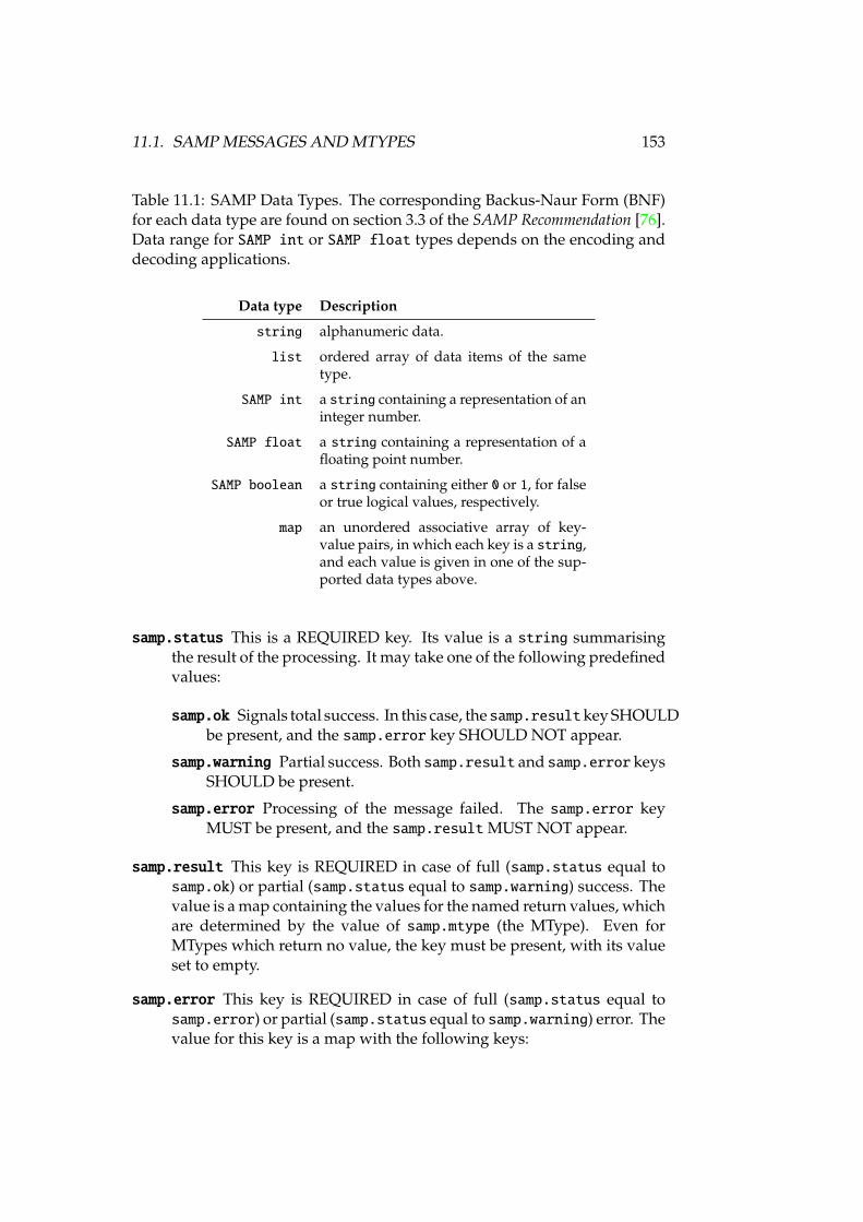
11.1. SAMP MESSAGES AND MTYPES 153
Table 11.1: SAMP Data Types. The corresponding Backus-Naur Form (BNF)for each data type are found on section 3.3 of the SAMP Recommendation [76].Data range for SAMP int or SAMP float types depends on the encoding anddecoding applications.
Data type Description
string alphanumeric data.
list ordered array of data items of the sametype.
SAMP int a string containing a representation of aninteger number.
SAMP float a string containing a representation of afloating point number.
SAMP boolean a string containing either 0 or 1, for falseor true logical values, respectively.
map an unordered associative array of key-value pairs, in which each key is a string,and each value is given in one of the sup-ported data types above.
samp.status This is a REQUIRED key. Its value is a string summarisingthe result of the processing. It may take one of the following predefinedvalues:
samp.ok Signals total success. In this case, thesamp.resultkey SHOULDbe present, and the samp.error key SHOULD NOT appear.
samp.warning Partial success. Both samp.result and samp.error keysSHOULD be present.
samp.error Processing of the message failed. The samp.error keyMUST be present, and the samp.result MUST NOT appear.
samp.result This key is REQUIRED in case of full (samp.status equal tosamp.ok) or partial (samp.status equal to samp.warning) success. Thevalue is a map containing the values for the named return values, whichare determined by the value of samp.mtype (the MType). Even forMTypes which return no value, the key must be present, with its valueset to empty.
samp.error This key is REQUIRED in case of full (samp.status equal tosamp.error) or partial (samp.status equal to samp.warning) error. Thevalue for this key is a map with the following keys:
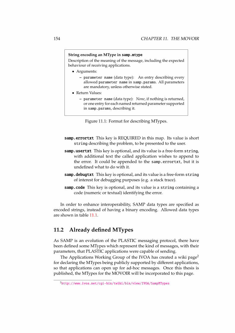
154 CHAPTER 11. THE MOVOIR
String encoding an MType in samp.mtypeDescription of the meaning of the message, including the expectedbehaviour of receiving applications.• Arguments:
– parameter name (data type): An entry describing everyallowed parameter name in samp.params. All parametersare mandatory, unless otherwise stated.
• Return Values:– parameter name (data type): None, if nothing is returned,
or one entry for each named returned parameter supportedin samp.params, describing it.
Figure 11.1: Format for describing MTypes.
samp.errortxt This key is REQUIRED in this map. Its value is shortstring describing the problem, to be presented to the user.
samp.usertxt This key is optional, and its value is a free-form string,with additional text the called application wishes to append tothe error. It could be appended to the samp.errortxt, but it isundefined what to do with it.
samp.debugtxt This key is optional, and its value is a free-form stringof interest for debugging purposes (e.g. a stack trace).
samp.code This key is optional, and its value is a string containing acode (numeric or textual) identifying the error.
In order to enhance interoperability, SAMP data types are specified asencoded strings, instead of having a binary encoding. Allowed data typesare shown in table 11.1.
11.2 Already defined MTypes
As SAMP is an evolution of the PLASTIC messaging protocol, there havebeen defined some MTypes which represent the kind of messages, with theirparameters, that PLASTIC applications were capable of sending.
The Applications Working Group of the IVOA has created a wiki page2
for declaring the MTypes being publicly supported by different applications,so that applications can open up for ad-hoc messages. Once this thesis ispublished, the MTypes for the MOVOIR will be incorporated to this page.
2http://www.ivoa.net/cgi-bin/twiki/bin/view/IVOA/SampMTypes
11.2. ALREADY DEFINED MTYPES 155
In particular, the following MTypes are the ones officially supported byclients such as TOPCAT and Aladin. They will be shown in the format offigure 11.1.
table.load.votable
Load (possibly display, or otherwise acknowledge the receipt of) atable in VOTable format.
• Arguments:
– url (string): URL of the VOTable document to load.– table-id (string) optional: identifier which may be used to
refer to the loaded table in subsequent messages.– name (string) optional: name which may be used to label
the loaded table in the application GUI.
• Return Values:
– none.
table.load.fits
Load (possibly display, or otherwise acknowledge the receipt of) adata table in FITS format.
• Arguments:
– url (string): URL of the FITS file to load.– table-id (string) optional: identifier which may be used to
refer to the loaded table in subsequent messages.– name (string) optional: name which may be used to label
the loaded table in the application GUI.
• Return Values:
– none.
table.highlight.row
Highlights a single row of an identified table by row index. Thetable to operate on is identified by one or both of the table-id orurl arguments. At least one of these must be supplied; if both aregiven they should refer to the same thing. Exactly what highlight-ing means is left to the receiving application.
• Arguments:
– table-id (string) optional, if url is specified: identifier as-sociated with a table, established by a previous message(e.g. table.load.*)
– url (string) optional, if table-id is specified: URL of a table.– row (SAMP int): Row index (zero-based) of the row to
highlight.
156 CHAPTER 11. THE MOVOIR
• Return Values:
– none.
table.select.rowList
Selects a list of rows of an identified table by row index. The tableto operate on is identified by one or both of the table-id or urlarguments. At least one of these must be supplied; if both aregiven they should refer to the same thing. Exactly what selectionmeans is left to the receiving application.
• Arguments:
– table-id (string) optional, if url is specified: identifier as-sociated with a table, established by a previous message(e.g. table.load.*)
– url (string) optional, if table-id is specified: URL of a table.– row (list of SAMP int): list of row indices (zero-based)
defining which table rows are to form the selection
• Return Values:
– none.
image.load.fits
Load (possibly display, or otherwise acknowledge) a two-dimensionalFITS image.
• Arguments:
– url (string): URL of the FITS image to be loaded.– image-id (string) optional: identifier which may be used to
refer to the loaded FITS image in subsequent messages.– name (string) optional: name which may be used to label
the loaded FITS image in the application GUI.
• Return Values:
– none.
coord.pointAt.sky
Directs attention (e.g. by moving a cursor or shifting the field ofview) to a given point on the celestial sphere.
• Arguments:
– ra (SAMP float): Right ascension in degrees.– dec (SAMP float): Declination in degrees.
• Return Values:
– none.

11.3. ALTERNATIVE RESPONSE PATTERNS 157
We can see in the message descriptions that applications developers’ flex-ibility is encouraged, but an additional property of all of these messages col-laborates in that flexibility: none of the MTypes above return anything, andthe application behaviour upon receipt of these messages can be completelyarbitrary.
We will use this flexibility to define a set of behaviours, upon receipt ofstandard MTypes, which will aid in calculations, and will provide the API forthe MOVOIR operations.
11.3 Alternative response patterns
We have seen in the previous section that there are a number of already stan-dardised MTypes, together with their corresponding responses upon receiptof those MTypes. For all of those messages applications returned nothing3,and there were clear indications that applications should perform certaintasks upon receipt of such MTypes, but there is nothing the caller applicationcan do in order to ensure a particular response, and this is a feature of thismessaging system: applications are notified of an event, and what to do uponreceiving it is completely up to them.
One clear case of SAMP-based application which subscribes to the mes-sages above, but does not really perform the actions specified by the MTypedescription, are logger application. A typical logger application would reg-ister with a SAMP hub, and subscribe to every possible message. However,for all messages received the message handler is the same, and just logs thesamp.mtype and samp.params of the call, together with information about thecaller application.
The lesson to learn from this example is that applications which subscribeto broadcasted messages, and specially those who require no answer, arecompletely transparent to caller applications: we can perform any actionit makes sense to perform upon receipt of these messages, as long as theformal behaviour expected by the calling application (in terms of answeringa synchronous message, not letting the calling application blocked, filling allrequired keywords in the response...) is fulfilled.
Let us explore a few examples of new functionality which can be addedby two means: performing a somewhat different action upon receiving oneof the standard messages, or letting called applications see who has calledthem, and send messages back to applications which support them.
3Formally, asynchronously called modules which return nothing SHOULD call the callers’replymethod with a mapwith keys samp.status set to samp.ok and samp.result set to empty,but applications SHOULD NOT behave incorrectly if they do not receive it.
158 CHAPTER 11. THE MOVOIR
Modifying or enhancing response actions
The first case (modifying what is done by the receiving applications) wasillustrated by our previous example of a logger application, and we will alsouse this way to create a VODownloader application.
A VODownloader is, essentially, an application which, instead of actuallyworking with the VOTables and FITS files which are sent to it, it down-loads them to a particular folder. This requires being able to respond tothe table.load.votable, table.load.fits, and image.load.fits, and usethe url parameter as a data source to download the file sent. This changessomehow the meaning of the table.load.* and image.load.fits MTypes,but in a sense which is compatible with the message definition, and providesa valuable service for integrating legacy applications for which there is noaccess to source code, and which cannot be integrated into the VO. For them,a VODownloader application is the only possible data access bridge to theVO.
Performing same message call-backs
When sending an asynchronous message, the caller application provides afunction the called service needs to call back in order to provide the actualresult.
However, that is only possible for asynchronous messages with MTypesexpecting return values, and none of the standard messages provide nothingback. Of course, we can create our own, custom MTypes, but those will onlybe useful for the subset of applications which known about those additionalMTypes. If we want to provide an extension mechanism for already existingVO applications, and for those applications whose only connection to the VOis messaging, we need to provide extensions through the existing MTypes.
Nonetheless, SAMP provides the mechanisms for that: as describedin section 3.12, a callable client must support the receiveNotification,receiveCall, and reply methods, and all of them receive a sender-id pa-rameter.
This allows called applications to send messages to the clients who calledthem first, upon receipt of a particular message.
In this way, we can think of different possibilities upon receipt of a givenMType which can be replied by sending back the same MType:
image.load.fits In this message, only the url parameter is mandatory.Upon receipt of such a message, the called module would perform someprocessing: for instance, image inversion, rotation, reflection, automaticlevel adjustments, adaptive wavelet filtering, FFTs, et cetera. Then, itwould send the application which sent the original message anotherimage.load.fits MType with the processed image.
11.3. ALTERNATIVE RESPONSE PATTERNS 159
table.load.votable Again, in this message only theurlparameter is manda-tory. Upon receipt of such a message, the called module would performsome processing: for instance, FFT of VOTable columns (in order toget spectra from auto-correlation data), statistics on the columns (min,max, average, median, standard deviation, et cetera), et cetera. Then,it would send the application which sent the original table anothertable.load.votable MType with the processed table.
In order for users to discover the actual behaviour of each module, theactual processing being performed (including default parameters being ap-plied) SHOULD be available via the samp.description metadata declaredwith the hub.
Performing different message call-backs
We are not restricted to create responses as messages of the same time tobe back to the calling client. We might have, for example, a module whichtakes an image.load.fits MType, and uses SExtractor4 to create a catalogueof sources detected on that FITS. The catalogue could be sent to other tableloading applications (e.g. TOPCAT, but it could be broadcast to all subscribersof the table.load.votable MType) for display via a table.load.votablemessage, or simple stored as a file in a particular folder.
Another interesting possibility is that of receiving ra and dec coordinatesvia a coords.pointAt.sky MType, and performing a ConeSearch query onthose coordinates for selected services, sending results back as atable.load.votablemessage.
With the schema described up to now we could only build modules limitedto process just one input, be it a table, an image, or a pair of coordinates.
However, we can push this concept further, so that SAMP modules whichneed to operate on two inputs would wait for two messages of the same typefrom the same client, with different data, in order to use both data inputs.
One such example would be a module for cross-matching sources fromtwo different catalogues. The sequence, in this case, would be:
1. An application (e.g. TOPCAT) sends a VOTable to an application (whichwe can call XMatch) which supports the table.load.votable MType.
2. XMatch starts preparing for a XMatch of that first table with anothertable yet to be sent by the same client.
3. The same application sends a second VOTable to the XMatch applicationvia the table.load.votable MType.
4http://terapix.iap.fr/soft/sextractor/
160 CHAPTER 11. THE MOVOIR
4. XMatch performs a cross-matching of both tables, using default param-eters, creating a third table, with all fields from both tables for sourceswhich were successfully cross-matched.
5. When the cross-matching table has been created, a message is sent tothe caller application using the same table.load.votable MType.
Such an XMatch module would be able to provide cross-matching ser-vices to every SAMP-enabled application able to send table.load.votableMTypes, as most applications being able to sendtable.load.votableMTypescan handle them as well. This means that just by supporting the standardmessages, applications can be enhanced by modules which can act upon re-ceipt of standard messages. We have, in fact, created a plug-in API for theVO.
This operation model has the drawback of needing a series of defaultparameters which cannot be specified by the calling applications, as they areusing a generic message for loading data.
That problem could be overcome in two ways: first, as the data is sent inthe VOTable format, if there are additional metadata on spatial resolution thecross-matching service could be able to adjust its default parameters from theavailable information.
Second, specially formatted VOTables could be sent to the modules via thesame table.load.votable messages. The formatting would include precisefield names corresponding to the parameters to be set for processing datafrom subsequent messages.
A final goal of these thesis would be the development of an IVOA-sanctioned plug-in architecture, were specific MTypes would be created forgetting application capabilities (default values set-up, methods for discoveryof plug-in messages, et cetera) the creation of MTypes specific for handlingthese module properties.
In that case, another tool which could be performed would be the auto-matic creation of messages for applications, by just selecting the message, andproviding links to the data being created.
In addition, by publishing into the IVOA wiki the messages used by theMOVOIR, they could become more generalised, and available from manymore modules.
11.4 MOVOIR modules
After having presented how different SAMP-based processing strategies canbe built, we will present here the different MOVOIR modules, and theircorresponding MTypes they support with the actual behaviour being imple-mented.

11.5. SALIENT FEATURES OF THE MOVOIR 161
In particular, we have implemented the modules which were suggestedin section 10.6 of the previous chapter:
11.5 Salient features of the MOVOIR
By the way it has been developed, the MOVOIR has the following properties:
Multi-language support Astronomical data tools used to be written in FOR-TRAN, and compiled for UNIX-like systems. As of late, many astro-nomical applications, specially if they need to communicate with theVO, are being written in Java or in advanced scripting languages suchas Python, which are available not only for UNIX-like systems, but forcommon platforms such as Windows or the Mac. The MOVOIR hasparts written in Java, and in Python, but the interface is common toany kind of application supporting XML-RPC calls. In particular, itwill support language-independent VO application messaging —seesection 2.7—.
Multi-platform support Stemming from the usage of platform neutral lan-guages, such as Java and Python, the MOVOIR can be used in everymajor platform (Linux, Mac, Windows), and in any other platform sup-porting any language with an XML-RPC library, or even just able tocreate communication sockets.
Reuse of existing packages The MOVOIR uses the STIL table library5 for itsinternal table operations, and the AstroRuntime (the server part of theVO Desktop) for VO query support. The application-specific part of theMOVOIR uses also the STIL table library and the nom.tam.fits6 Javalibrary for Java applications, and the standalone STILTS package7 andthe PyFITS8 for Python applications. This allows for the combination ofMOVOIR features with those independently exposed by the STIL andAstroRuntime, and the combination of scripts supporting both toolswith those making use of MOVOIR’s capabilities.
Single-operation, Multiple-targets The MOVOIR is able to work on multi-ple targets as the same time in every function which would normallyexpect a single target. This allows more complex workflows to be built,and to enhance query throughput.
Data Oriented Interface Most VO applications tend to be built around theexisting Data Access Layer, or the VO protocols used for data access.
5http://www.star.bristol.ac.uk/~mbt/stil/6http://heasarc.gsfc.nasa.gov/docs/heasarc/fits/java/v0.9/7http://www.star.bristol.ac.uk/~mbt/stilts/8http://www.stsci.edu/resources/software_hardware/pyfits
162 CHAPTER 11. THE MOVOIR
They also treat the coordinate resolution systems such as Sesame, orRegistry queries, as separate parts of the system. The MOVOIR interfaceis data focused, and filtering is performed from the coordinates first,with particular queries fitted to each particular service. This is also truefor the scripting interface.
Dynamic module update As the MOVOIR uses a hub based mechanismfor module registration, modules can be added or removed dynami-cally, and SAMP-enabled applications expect registered applications tochange over time. This makes modules newly registered with the hubavailable to all applications able to send the MTypes the new modulesare subscribed to. This feature eases development, deployment, andthe updating of the MOVOIR, or any other SAMP-based package.
Message based API As the MOVOIR uses the Simple Application Messag-ing Protocol (SAMP) as the main interaction bus, all operation requestsare sent as SAMP messages, and the synchronous or asynchronous re-sponses are also in the form of SAMP messages. This decision allows forthe definition of an initial plug-in API which is message-based, insteadof language- or library-based.
11.6 Main issues
We will review the main issues with the MOVOIR in this section.
SAMP UI scalability
The main problem with the MOVOIR is its scalability as a plug-in API. Asthe number of modules included with the MOVOIR, together with SAMPapplications, increases, so does the time needed by the user to find the correctmodule for sending the data.
The modularity of the MOVOIR helps, as modules do not need to rununtil needed, and are available right after launch, but still the problem ofa likely increase of the number of SAMP-enabled applications and modulesremains.
Possible UI solutions to that problem would be:
SAMP specific communication panes Instead of using a simple pop-up menu,a SAMP-specific pane could be used, either as a floating or auxiliarywindow, or as a pop-up drawer, which allowed for a better access tometadata descriptions not just in the hub UI, but also in the client.
11.7. CONCLUSIONS 163
High delay, unexpected responses
Some users might think that the MOVOIR can create “non-causal” responses.That is, users might send a message to a module which takes a long processingtime, and even reiterate the message, and then the application they are usingmight show two tables, or two images, that they are no longer expecting.
In order to avoid this processing time should be less than real time ex-pectations. The typical golden rule for interactive systems is delivering aresponse in under 8 to 15 seconds9. Independently of the actual value, re-sponses taking longer than that threshold might be thought as unrelated tothe initiating task, startling users. In any case, systems taking longer than oneminute to process data should use messaging just to retrieve data, providingtheir own UI to initiate the processing, giving information on lead time forthe tasks.
11.7 Conclusions
In this chapter we have shown how a data processing API can be built on topof the SAMP messaging protocol, and what ideas can be developed in orderto create an extension mechanism for already existing VO applications.
The main achievement for the MOVOIR, being based on SAMP, is that itprovides a way to create plug-ins for existing VO applications, which can bemade independent of both the platform and language those modules can bewritten into, and completely independent of applications being enhanced.
9http://www.ariadneproject.org/index.php?id=63

Part IV
Thesis applications
165

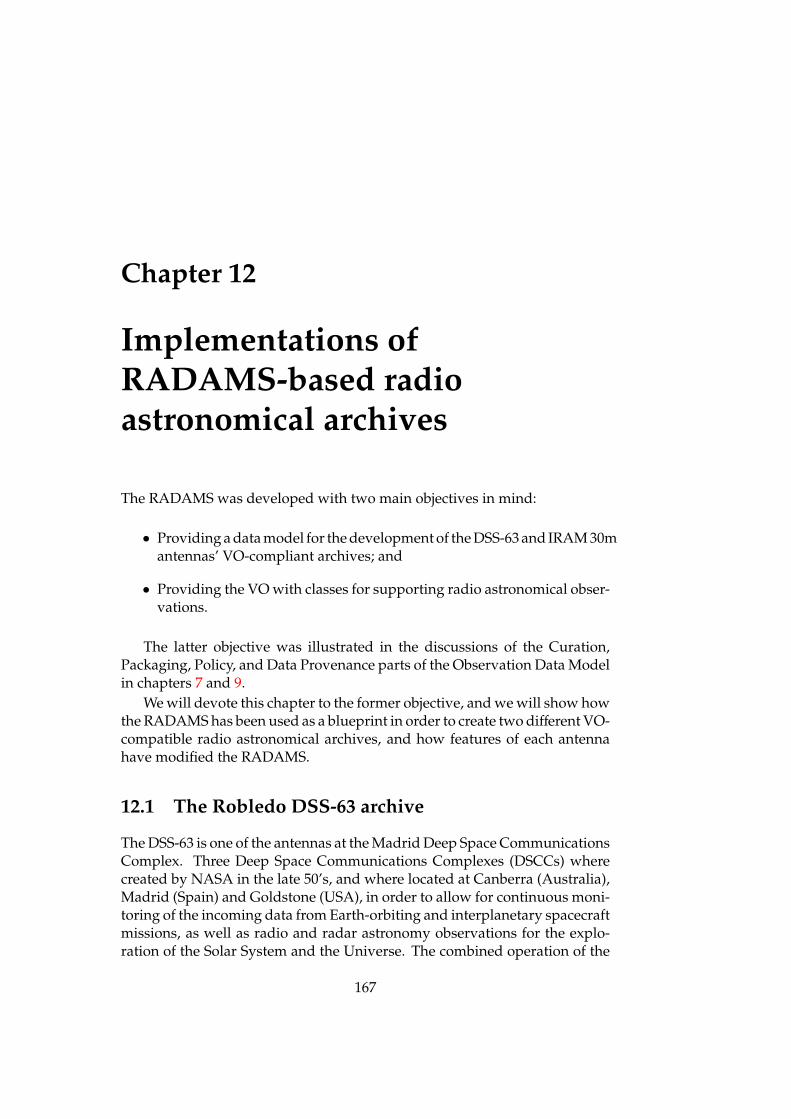
Chapter 12
Implementations ofRADAMS-based radioastronomical archives
The RADAMS was developed with two main objectives in mind:
• Providing a data model for the development of the DSS-63 and IRAM 30mantennas’ VO-compliant archives; and
• Providing the VO with classes for supporting radio astronomical obser-vations.
The latter objective was illustrated in the discussions of the Curation,Packaging, Policy, and Data Provenance parts of the Observation Data Modelin chapters 7 and 9.
We will devote this chapter to the former objective, and we will show howthe RADAMS has been used as a blueprint in order to create two different VO-compatible radio astronomical archives, and how features of each antennahave modified the RADAMS.
12.1 The Robledo DSS-63 archive
The DSS-63 is one of the antennas at the Madrid Deep Space CommunicationsComplex. Three Deep Space Communications Complexes (DSCCs) wherecreated by NASA in the late 50’s, and where located at Canberra (Australia),Madrid (Spain) and Goldstone (USA), in order to allow for continuous moni-toring of the incoming data from Earth-orbiting and interplanetary spacecraftmissions, as well as radio and radar astronomy observations for the explo-ration of the Solar System and the Universe. The combined operation of the
167
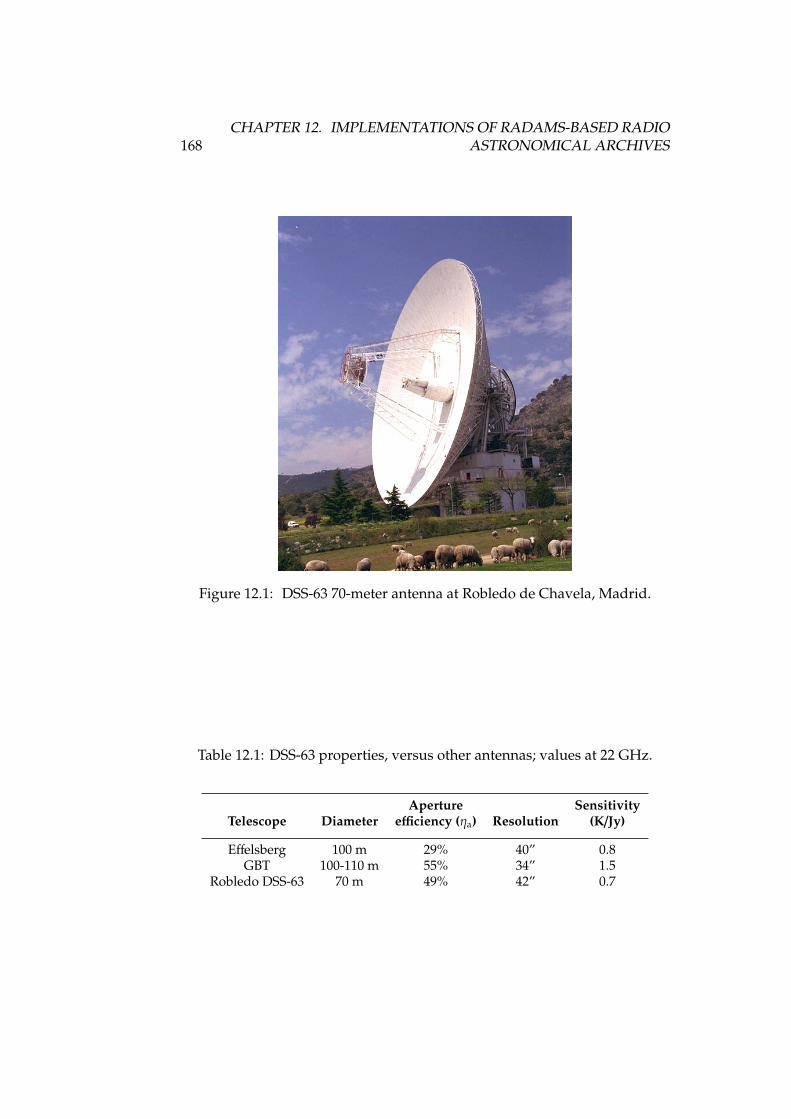
168CHAPTER 12. IMPLEMENTATIONS OF RADAMS-BASED RADIO
ASTRONOMICAL ARCHIVES
Figure 12.1: DSS-63 70-meter antenna at Robledo de Chavela, Madrid.
Table 12.1: DSS-63 properties, versus other antennas; values at 22 GHz.
Aperture SensitivityTelescope Diameter efficiency (ηa) Resolution (K/Jy)
Effelsberg 100 m 29% 40” 0.8GBT 100-110 m 55% 34” 1.5
Robledo DSS-63 70 m 49% 42” 0.7
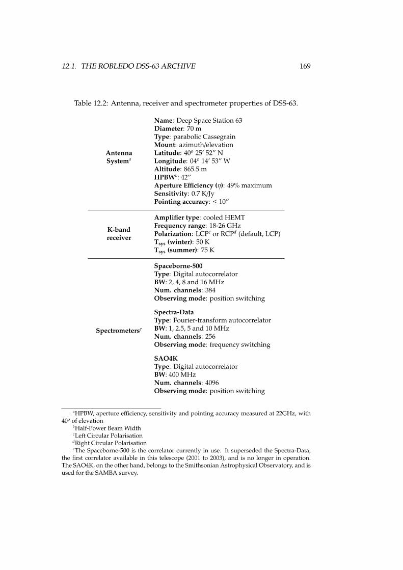
12.1. THE ROBLEDO DSS-63 ARCHIVE 169
Table 12.2: Antenna, receiver and spectrometer properties of DSS-63.
AntennaSystema
Name: Deep Space Station 63Diameter: 70 mType: parabolic CassegrainMount: azimuth/elevationLatitude: 40o 25’ 52” NLongitude: 04o 14’ 53” WAltitude: 865.5 mHPBWb: 42”Aperture Efficiency (η): 49% maximumSensitivity: 0.7 K/JyPointing accuracy: ≤ 10”
K-bandreceiver
Amplifier type: cooled HEMTFrequency range: 18-26 GHzPolarization: LCPc or RCPd (default, LCP)Tsys (winter): 50 KTsys (summer): 75 K
Spectrometerse
Spaceborne-500Type: Digital autocorrelatorBW: 2, 4, 8 and 16 MHzNum. channels: 384Observing mode: position switching
Spectra-DataType: Fourier-transform autocorrelatorBW: 1, 2.5, 5 and 10 MHzNum. channels: 256Observing mode: frequency switching
SAO4KType: Digital autocorrelatorBW: 400 MHzNum. channels: 4096Observing mode: position switching
aHPBW, aperture efficiency, sensitivity and pointing accuracy measured at 22GHz, with40o of elevation
bHalf-Power Beam WidthcLeft Circular PolarisationdRight Circular PolarisationeThe Spaceborne-500 is the correlator currently in use. It superseded the Spectra-Data,
the first correlator available in this telescope (2001 to 2003), and is no longer in operation.The SAO4K, on the other hand, belongs to the Smithsonian Astrophysical Observatory, and isused for the SAMBA survey.
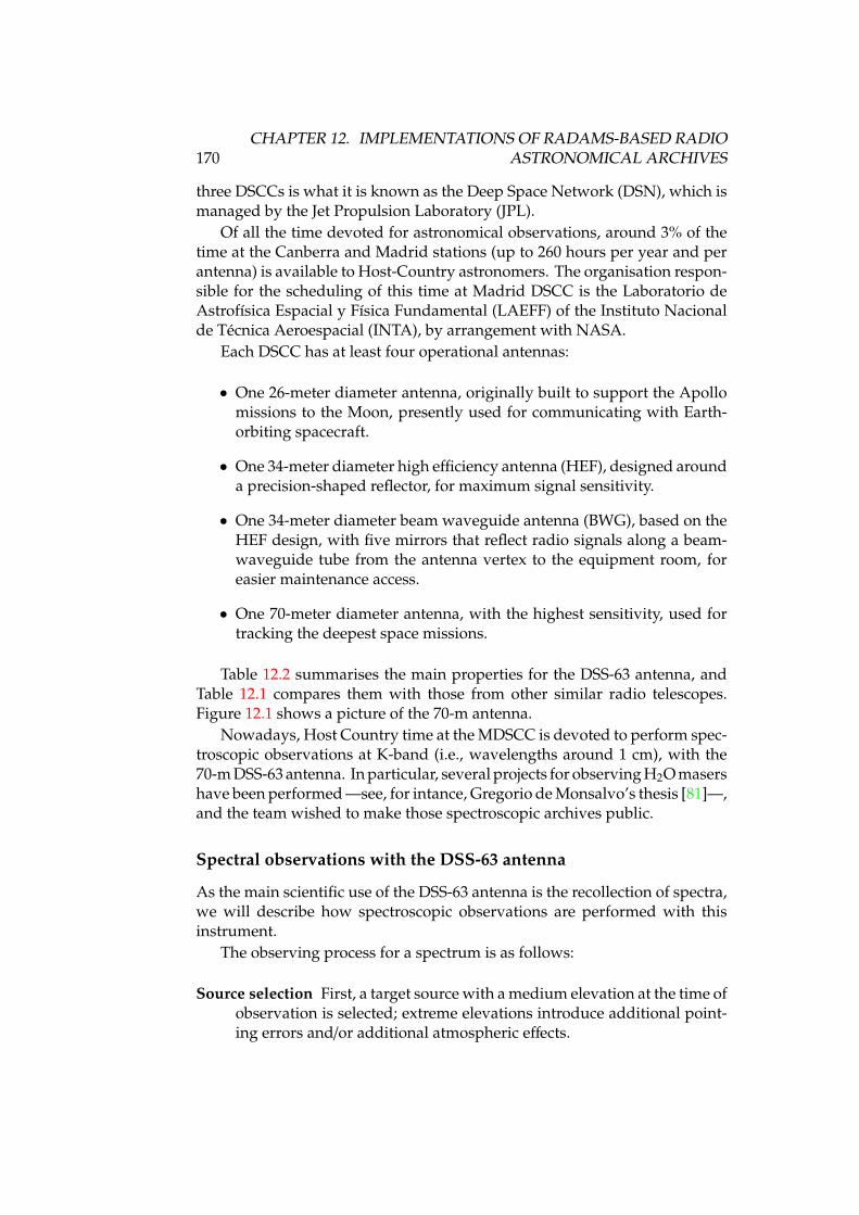
170CHAPTER 12. IMPLEMENTATIONS OF RADAMS-BASED RADIO
ASTRONOMICAL ARCHIVES
three DSCCs is what it is known as the Deep Space Network (DSN), which ismanaged by the Jet Propulsion Laboratory (JPL).
Of all the time devoted for astronomical observations, around 3% of thetime at the Canberra and Madrid stations (up to 260 hours per year and perantenna) is available to Host-Country astronomers. The organisation respon-sible for the scheduling of this time at Madrid DSCC is the Laboratorio deAstrofísica Espacial y Física Fundamental (LAEFF) of the Instituto Nacionalde Técnica Aeroespacial (INTA), by arrangement with NASA.
Each DSCC has at least four operational antennas:
• One 26-meter diameter antenna, originally built to support the Apollomissions to the Moon, presently used for communicating with Earth-orbiting spacecraft.
• One 34-meter diameter high efficiency antenna (HEF), designed arounda precision-shaped reflector, for maximum signal sensitivity.
• One 34-meter diameter beam waveguide antenna (BWG), based on theHEF design, with five mirrors that reflect radio signals along a beam-waveguide tube from the antenna vertex to the equipment room, foreasier maintenance access.
• One 70-meter diameter antenna, with the highest sensitivity, used fortracking the deepest space missions.
Table 12.2 summarises the main properties for the DSS-63 antenna, andTable 12.1 compares them with those from other similar radio telescopes.Figure 12.1 shows a picture of the 70-m antenna.
Nowadays, Host Country time at the MDSCC is devoted to perform spec-troscopic observations at K-band (i.e., wavelengths around 1 cm), with the70-m DSS-63 antenna. In particular, several projects for observing H2O masershave been performed —see, for intance, Gregorio de Monsalvo’s thesis [81]—,and the team wished to make those spectroscopic archives public.
Spectral observations with the DSS-63 antenna
As the main scientific use of the DSS-63 antenna is the recollection of spectra,we will describe how spectroscopic observations are performed with thisinstrument.
The observing process for a spectrum is as follows:
Source selection First, a target source with a medium elevation at the time ofobservation is selected; extreme elevations introduce additional point-ing errors and/or additional atmospheric effects.
12.1. THE ROBLEDO DSS-63 ARCHIVE 171
Pointing calibrator selection Once the source has been selected, a strongpointing calibration source near the target is chosen, because minimis-ing antenna motion1 between pointing calibration and the actual obser-vation better maintains the mirror shape.
Pointing calibration The antenna will be moved up and down in elevation,and clockwise and counter-clockwise in cross-elevation, around theexpected position for the pointing calibrator. As the profile for thetelescope beam conforms to a Gaussian distribution, the data can befitted with a Gaussian, and the pointing error adjusted by comparisonbetween the expected position of the calibrator, and the fitted maximumflux position. This correction will be applied to the coordinates wherethe source is expected to be.
Focus calibration The same calibrator can be used to calibrate the focus ofthe instrument, defined as the position of the secondary mirror thatmaximises the power collected by the instrument. Again, the profilefor the focus, when the mirror is moved along its axis, is assumed to beGaussian, and the fit for the maximum provides the focus.
On/Off source observation Both the source and a nearby position with noemissions have to be observed, in order to discriminate the contributionfrom the instrument. This is performed either by changing the positionof the antenna (position switching), or by moving the secondary mirrorin such a way that the main feed is focused on a different region of thesky, with no radio sources (wobbler switching). Another possibility isto compare the power of the emission from the same source at slightlydifferent frequencies, assuming that the antenna and atmospheric noisedoes not change with this frequency switch (frequency switching). Inthe case of the DSS-63, on/off observations are performed either byposition switching or frequency switching.
Atmospheric corrections The amount of energy received by the instrumentdepends strongly on weather conditions, and on the length of the pathof the signal through the atmosphere. In particular, at cm wavelengthsthe amount of water vapour in the atmosphere is the major contributorto atmospheric opacity (a quantity that is proportional to the proba-bility of a photon being absorbed after travelling a given length in theatmosphere). Measurements of opacity at different elevations (tippingcurves, or skydips), which correspond to different air masses (a measureof the amount of atmospheric gas in the line of sight of the instrument),are used to fit a curve that provides the atmospheric opacity2. This isusually done at DSS-63 once per observing session and frequency setup.
1specially in elevation2See section 7.2 in Tools of radio astronomy [82] for details.
172CHAPTER 12. IMPLEMENTATIONS OF RADAMS-BASED RADIO
ASTRONOMICAL ARCHIVES
There are other corrections and calibrations to consider, but most of themcan be obtained from typical values for the instrument and particular con-figuration, and do not contribute to illustrate the observing process with theDSS-63 antenna.
Of particular interest will be parameters such as system temperature (Tsys),main beam solid angle (Ωmb), aperture efficiency (ηa), and the antenna tem-perature scale.
The data output of the correlator is a 384-sample autocorrelation function,which by means of the Fourier transform (Discrete Fourier Transform, in thiscase) provides a function proportional to the power spectrum of the source3.The post-processing of the observation, together with the calibration proce-dures, will allow us to determine the actual spectrum scale, and frequenciesfor the salient features of the spectrum.
Archive requirements
The archive for the DSS-63 antenna, then, is an archive for single-point spec-troscopic observations. The particular requirements for the archive were:
Support for two single-point modes The DSS-63 antenna archive would hold,as per the initial specification, only single-point on-off spectra using fre-quency switching, or single-point continuum measurements.
VO spectral access services The main data products of the archive are spec-tra, which are supported by the Spectrum Data Model (incorporated inthe RADAMS, as we have seen), and continuum measurements, whichare considered to be one-point, wide-band spectra, similar to photomet-ric data points in the visible band. A SSAP service will be implementedon top of the database.
Web access interface The web access interface would use the same infras-tructure needed for the SSAP service, but providing.
No modification to the instrument control system All of the information storedin the archive should be available either from ingestion of the FITS files,or by harvesting the observation logs and control system output, butnothing should be added to the instrument control system. This is botha precautionary measure, so that we do not interfere with the telescope,but also works for making the project self-contained: tasks can be per-formed without need for external developers to modify another pieceof software.
Simple data access policy The data access policy of application to the archiveis the straightforward NRAO policy: after 18 months, data are available
3See section 4.1.2 of Tools of Radio Astronomy [82] for the derivation.
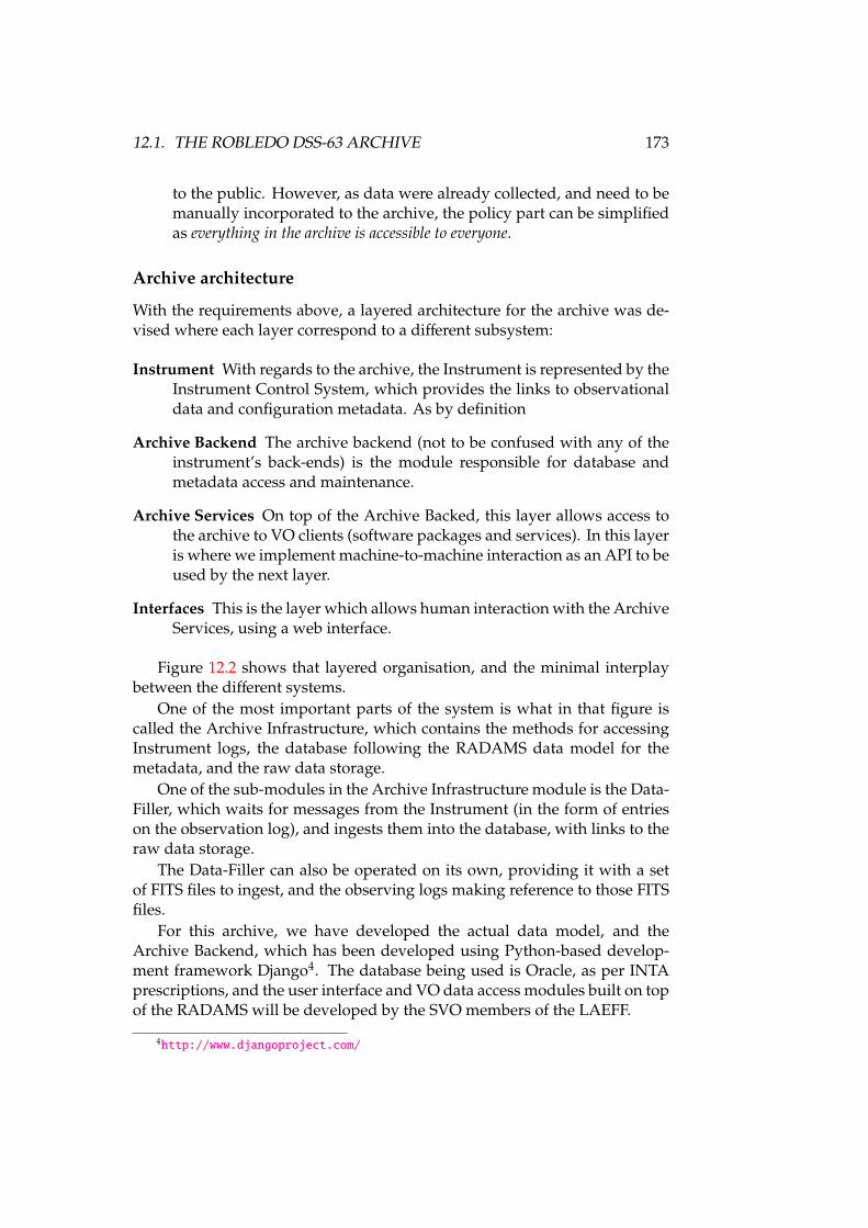
12.1. THE ROBLEDO DSS-63 ARCHIVE 173
to the public. However, as data were already collected, and need to bemanually incorporated to the archive, the policy part can be simplifiedas everything in the archive is accessible to everyone.
Archive architecture
With the requirements above, a layered architecture for the archive was de-vised where each layer correspond to a different subsystem:
Instrument With regards to the archive, the Instrument is represented by theInstrument Control System, which provides the links to observationaldata and configuration metadata. As by definition
Archive Backend The archive backend (not to be confused with any of theinstrument’s back-ends) is the module responsible for database andmetadata access and maintenance.
Archive Services On top of the Archive Backed, this layer allows access tothe archive to VO clients (software packages and services). In this layeris where we implement machine-to-machine interaction as an API to beused by the next layer.
Interfaces This is the layer which allows human interaction with the ArchiveServices, using a web interface.
Figure 12.2 shows that layered organisation, and the minimal interplaybetween the different systems.
One of the most important parts of the system is what in that figure iscalled the Archive Infrastructure, which contains the methods for accessingInstrument logs, the database following the RADAMS data model for themetadata, and the raw data storage.
One of the sub-modules in the Archive Infrastructure module is the Data-Filler, which waits for messages from the Instrument (in the form of entrieson the observation log), and ingests them into the database, with links to theraw data storage.
The Data-Filler can also be operated on its own, providing it with a setof FITS files to ingest, and the observing logs making reference to those FITSfiles.
For this archive, we have developed the actual data model, and theArchive Backend, which has been developed using Python-based develop-ment framework Django4. The database being used is Oracle, as per INTAprescriptions, and the user interface and VO data access modules built on topof the RADAMS will be developed by the SVO members of the LAEFF.
4http://www.djangoproject.com/
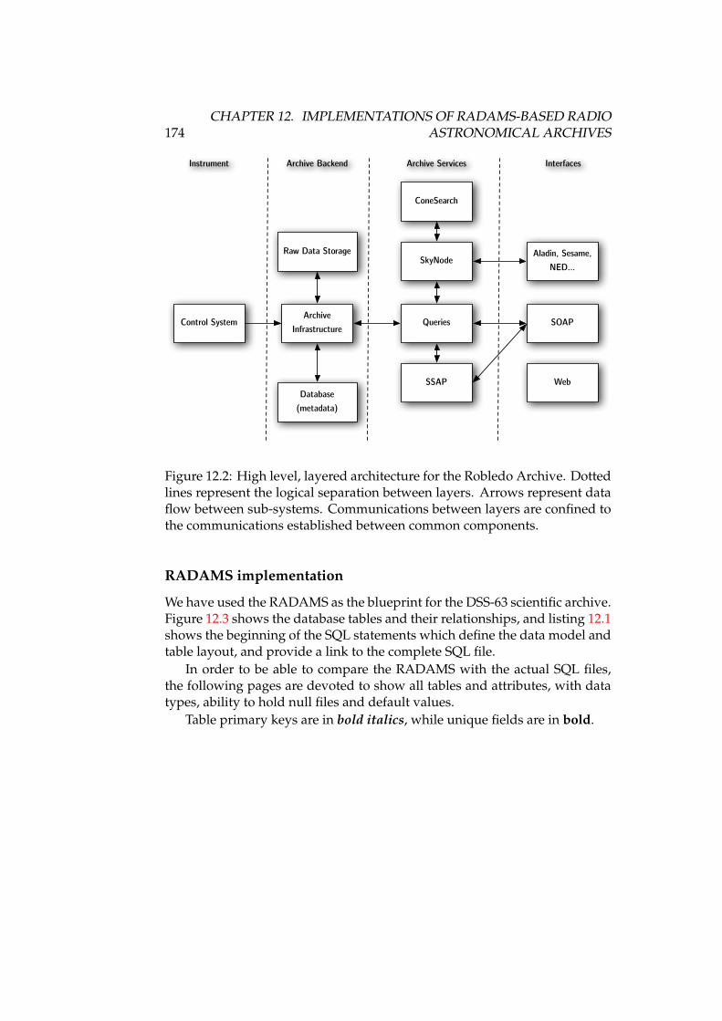
174CHAPTER 12. IMPLEMENTATIONS OF RADAMS-BASED RADIO
ASTRONOMICAL ARCHIVES
Database (metadata)
Queries
SkyNode
ConeSearch
SSAP
Control SystemArchive
Infrastructure
Raw Data Storage
Instrument Archive Backend Archive Services Interfaces
Aladin, Sesame, NED…
SOAP
Web
Figure 12.2: High level, layered architecture for the Robledo Archive. Dottedlines represent the logical separation between layers. Arrows represent dataflow between sub-systems. Communications between layers are confined tothe communications established between common components.
RADAMS implementation
We have used the RADAMS as the blueprint for the DSS-63 scientific archive.Figure 12.3 shows the database tables and their relationships, and listing 12.1shows the beginning of the SQL statements which define the data model andtable layout, and provide a link to the complete SQL file.
In order to be able to compare the RADAMS with the actual SQL files,the following pages are devoted to show all tables and attributes, with datatypes, ability to hold null files and default values.
Table primary keys are in bold italics, while unique fields are in bold.
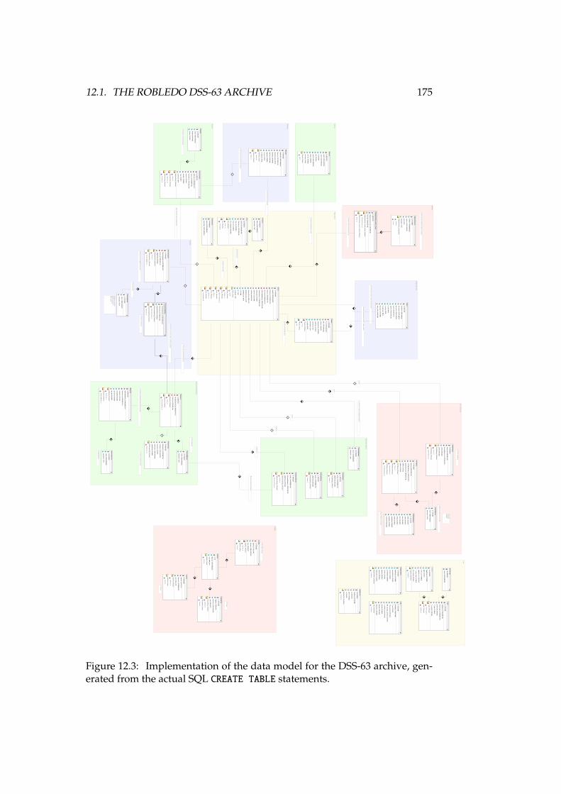
12.1. THE ROBLEDO DSS-63 ARCHIVE 175
Datafiller
Sources
Subscans
Scans related
Observation S
ettings
Receivers and B
ackends
Softw
are
Antenna
OTF and O
n/Off
Sw
itching
django.auth.users
Logs
horizontal projection nasm
yth
Frequency switching
Wobbler sw
itching B
eam sw
itching Total pow
er
Rel_37
FITS files
FITS files
AS
CII files from
logs
Rel_37
Fluxes for scans
Quality of scan data
Each scan has antenna param
eters
Sw
itching values applied in the scan
A scan m
ay use several receivers
Softw
are versions used in the scan
Calibrations
Pointing
OTF
Position S
witching
OnO
ff
Focus
A scan has several subscans
Rel_36
Receivers could have a freq. sw
itching applied
Map settings for the offset
Reference system
for the offset
Sources are observed in scans
Extensible to several antennas
Each subscan has antenna param
eters
One user (astronom
er) made the observation
Receiver used for calibration
List of Backends
Frequency Sw
itchingFrequency and Line N
ame
List of receivers
Sw
itching modes
A scan has an O
bserving Mode assigned
One user (astronom
er) is the P.I. of the project
A project has several scans
A receiver is filtered by m
any backends band
Static table w
ith different software versions
LogsExp
id: INTE
GE
R
timeS
tamp: D
ATE
TIME
gain: DO
UB
LE
linear_corr: DO
UB
LE
quadratic_corr: DO
UB
LE
T_noise_diode: DO
UB
LE
non_linearity: DO
UB
LE
LogsExp_tim
eStam
p
timeS
tamp
reducedFiles
id: INTE
GE
R
logFiles_id: INT (FK
)
filename: V
AR
CH
AR
(255)
year: SM
ALLIN
T
reducedFiles_FKIndex1
logFiles_id
reducedFiles_Unique
filename
rawFiles
id: INTE
GE
R
logFiles_id: INT (FK
)
filename: V
AR
CH
AR
(255)
year: SM
ALLIN
T
rawFiles_FK
Index1
logFiles_id
rawFiles_U
nique
filename
expFiles
id: INTE
GE
R
logFiles_id: INT (FK
)
filename: V
AR
CH
AR
(255)
year: SM
ALLIN
T
expFiles_FKIndex1
logFiles_id
expFiles_Unique
filename
logFiles
id: INT
filename: V
AR
CH
AR
(255)
year: SM
ALLIN
T
logFiles_Unique
filename
FluxUnits
id: INTE
GE
R
name: V
AR
CH
AR
(255)
description: TEX
T
SourceLogs
id: INTE
GE
R
name: V
AR
CH
AR
(255)
Logsid: INTE
GE
R
timeS
tamp: TIM
ES
TAM
P
T_lna: DO
UB
LE
T_fo_assumed: D
OU
BLE
ND
_coupling_correction: DO
UB
LE
T_ambient_load: D
OU
BLE
Azim
uth: DO
UB
LE
Elevation: D
OU
BLE
Frequency: DO
UB
LE
Logs_timeStam
p
timeS
tamp
LogsTid: INTE
GE
R
LogsExp_id: IN
TEG
ER
(FK)
SourceLogs_id: IN
TEG
ER
(FK)
powerm
eter: DO
UB
LE
T_linear: DO
UB
LE
T_corrected: DO
UB
LE
LogsT_FKIndex1
SourceLogs_id
LogsT_FKIndex2
LogsExp_id
Flux
id: INTE
GE
R
Scans_id: IN
TEG
ER
(FK)
FluxUnits_id: IN
TEG
ER
(FK)
Flux_max: D
OU
BLE
Flux_min: D
OU
BLE
Flux_integrated: DO
UB
LE
Flux_FKIndex1
Scans_id
Flux_FKIndex2
FluxUnits_id
ScansQ
uality
id: INTE
GE
R
name: V
AR
CH
AR
(255)
description: VA
RC
HA
R(255)
OnO
ffSettings
id: INTE
GE
R
Scans_id: IN
TEG
ER
(FK)
System
Nam
es_id: INTE
GE
R (FK
)
xOffset: D
OU
BLE
yOffset: D
OU
BLE
OnOffSettings_FK
Index1
Scans_id
OnOffSettings_FK
Index2
System
Nam
es_id
Antennas
id: INTE
GE
R
name: V
AR
CH
AR
(255)
longitude: DO
UB
LE
latitude: DO
UB
LE
OTFM
apSettings
id: INTE
GE
R
xStart: D
OU
BLE
yStart: D
OU
BLE
xEnd: D
OU
BLE
yEnd: D
OU
BLE
xStep: D
OU
BLE
yStep: D
OU
BLE
speedStart: D
OU
BLE
speedEnd: D
OU
BLE
timeP
erOtf: D
OU
BLE
PointingS
ettings
id: INTE
GE
R
Scans_id: IN
TEG
ER
(FK)
addedFields: DO
UB
LE
PointingS
ettings_FKIndex1
Scans_id
FocusSettings
id: INTE
GE
R
Scans_id: IN
TEG
ER
(FK)
addedFields: DO
UB
LE
FocusSettings_FK
Index1
Scans_id
CalibrationS
ettings
id: INTE
GE
R
Scans_id: IN
TEG
ER
(FK)
ReceiversN
ames_id: IN
TEG
ER
(FK)
addedFields: DO
UB
LE
CalibrationS
ettings_FKIndex1
Scans_id
CalibrationS
ettings_FKIndex2
ReceiversN
ames_id
OTFO
ffsets
id: INTE
GE
R
Scans_id: IN
TEG
ER
(FK)
OTFM
apSettings_id: IN
TEG
ER
(FK)
System
Nam
es_id: INTE
GE
R (FK
)
xOffset: D
OU
BLE
yOffset: D
OU
BLE
OTFO
ffsets_FKIndex1
Scans_id
OTFO
ffsets_FKIndex2
System
Nam
es_id
OTFO
ffsets_FKIndex3
OTFM
apSettings_id
System
Nam
es
id: INTE
GE
R
name: V
AR
CH
AR
(255)
description: TEX
T
BackendsN
ames
id: INTE
GE
R
name: V
AR
CH
AR
(255)
description: TEX
T
FrequencySw
itching
Sw
itchingValues_id: IN
TEG
ER
(FK)
Receivers_id: IN
TEG
ER
(FK)
frequencyThrow: D
OU
BLE
FrequencySwitching_FK
Index1
Sw
itchingValues_id
FrequencySwitching_FK
Index2
Receivers_id
ReceiversC
fg
id: INTE
GE
R
Receivers_id: IN
TEG
ER
(FK)
lineNam
e: VA
RC
HA
R(255)
frequency: DO
UB
LE
polarization: VA
RC
HA
R(255)
addedFields: DO
UB
LE
RxReceiversC
fg_FKIndex1
Receivers_id
ReceiversN
ames
id: INTE
GE
R
name: V
AR
CH
AR
(255)
description: TEX
T
Sw
itchingValues
id: INTE
GE
R
Sw
itchingModes_id: IN
TEG
ER
(FK)
Scans_id: IN
TEG
ER
(FK)
addedFields: DO
UB
LE
SwitchingV
alues_FKIndex1
Scans_id
SwitchingV
alues_FKIndex2
Sw
itchingModes_id
WeatherTau
id: INTE
GE
R
timeS
tamp: D
ATE
TIME
tau: DO
UB
LE
sigma: D
OU
BLE
fit: DO
UB
LE
WeatherTau_tim
eStam
p
timeS
tamp
WeatherS
tation
id: INTE
GE
R
timeS
tamp: D
ATE
TIME
electricalField: DO
UB
LE
windV
el: DO
UB
LE
windV
elMax: D
OU
BLE
windD
ir: DO
UB
LE
humidity: D
OU
BLE
pressure: DO
UB
LE
temperature: D
OU
BLE
WeatherS
tation_timeStam
p
timeS
tamp
Sw
itchingModes
id: INTE
GE
R
name: V
AR
CH
AR
(255)
description: TEX
T
ObservingM
odes
id: INTE
GE
R
name: V
AR
CH
AR
(255)
description: TEX
T
AntennaC
onfig
id: INTE
GE
R
Antennas_id: IN
TEG
ER
(FK)
Scans_id: IN
TEG
ER
(FK)
Subscans_id: IN
TEG
ER
(FK)
azimuth: D
OU
BLE
elevation: DO
UB
LE
Tsys: DO
UB
LE
comm
ents: TEX
T
AntennaC
onfig_FKIndex1
Scans_id
AntennaC
onfig_FKIndex2
Subscans_id
AntennaC
onfig_FKIndex3
Antennas_id
Usersid: IN
TEG
ER
username: V
AR
CH
AR
(30)
first_name: V
AR
CH
AR
(30)
last_name: V
AR
CH
AR
(30)
email: V
AR
CH
AR
(75)
passwd: V
AR
CH
AR
(128)
is_staff: BO
OL
is_active: BO
OL
is_superuser: BO
OL
last_login: DA
TETIM
E
date_joined: DA
TETIM
E
Backends
id: INTE
GE
R
BackendsN
ames_id: IN
TEG
ER
(FK)
Receivers_id: IN
TEG
ER
(FK)
resolution: DO
UB
LE
bandwidth: D
OU
BLE
spb_temp: D
OU
BLE
spb_pwr: D
OU
BLE
Backends_FK
Index1
Receivers_id
Backends_FK
Index2
BackendsN
ames_id
Receivers
id: INTE
GE
R
ReceiversN
ames_id: IN
TEG
ER
(FK)
Scans_id: IN
TEG
ER
(FK)
Receivers_FK
Index1
Scans_id
Receivers_FK
Index2
ReceiversN
ames_id
Subscans
id: INTE
GE
R
subscanID: V
AR
CH
AR
(255)
Scans_id: IN
TEG
ER
(FK)
dateObservation: D
ATE
startTime: D
ATE
TIME
endTime: D
ATE
TIME
exposure: DO
UB
LE
is_source: BO
OL
is_reference: BO
OL
Subscans_U
nique
subscanID
Subscans_FK
Index1
Scans_id
Softw
areVersions_used_in_S
cans
id: INTE
GE
R
Softw
areVersions_id: IN
TEG
ER
(FK)
Scans_id: IN
TEG
ER
(FK)
Softw
areVersions_usedin_S
cans_FKIndex1
Softw
areVersions_id
Softw
areVersions_used_in_S
cans_FKIndex3
Scans_id
Sources
id: INTE
GE
R
object: VA
RC
HA
R(255)
name: V
AR
CH
AR
(255)
ra: DO
UB
LE
dec: DO
UB
LE
epoch: VA
RC
HA
R(255)
deltav: DO
UB
LE
velo_lsr: DO
UB
LE
comm
ents: TEX
T
Sources_U
nique
object
Softw
areVersions
id: INTE
GE
R
software: V
AR
CH
AR
(255)
version: VA
RC
HA
R(255)
date: DA
TE
description: TEX
T
softwareV
ersions_uniqueswVer
software
version
Projects
id: INTE
GE
R
PI_id: IN
TEG
ER
(FK)
title: VA
RC
HA
R(255)
priority: INTE
GE
R
allocatedTime: D
OU
BLE
usedTime: D
OU
BLE
comm
ents: TEX
T
description: TEX
T
is_public: BO
OL
Projects_FK
Index1
PI_id
Projects_U
nique
title
Scansid: IN
TEG
ER
scanID: V
AR
CH
AR
(255)
Projects_id: IN
TEG
ER
(FK)
Users_id: IN
TEG
ER
(FK)
Sources_id: IN
TEG
ER
(FK)
ObservingM
odes_id: INTE
GE
R (FK
)
ScansQ
uality_id: INTE
GE
R (FK
)
nSubscans: IN
TEG
ER
startTime: D
ATE
TIME
endTime: D
ATE
TIME
observedTime: S
MA
LLINT
dateObservation: D
ATE
dateReduction: D
ATE
LST: TIM
E
UT: TIM
E
comm
ents: TEX
T
Scans_U
nique
scanID
Scans_FK
Index1
Projects_id
Scans_FK
Index2
ObservingM
odes_id
Scans_FK
Index3
Users_id
Scans_FK
Index4
Sources_id
Scans_FK
Index5
ScansQ
uality_id
1
Figure 12.3: Implementation of the data model for the DSS-63 archive, gen-erated from the actual SQL CREATE TABLE statements.
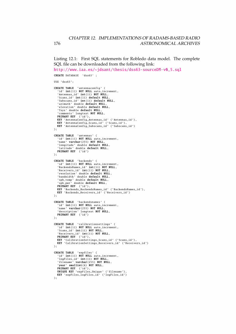
176CHAPTER 12. IMPLEMENTATIONS OF RADAMS-BASED RADIO
ASTRONOMICAL ARCHIVES
Listing 12.1: First SQL statements for Robledo data model. The completeSQL file can be downloaded from the following link:http://www.iaa.es/~jdsant/thesis/dss63-sourceDM-v0_5.sqlCREATE DATABASE ‘dss63‘ ;
USE ‘dss63‘;
CREATE TABLE ‘antennaconfig ‘ (‘id‘ int(11) NOT NULL auto_increment ,‘Antennas_id ‘ int(11) NOT NULL,‘Scans_id ‘ int(11) default NULL,‘Subscans_id ‘ int(11) default NULL,‘azimuth‘ double default NULL,‘elevation ‘ double default NULL,‘Tsys‘ double default NULL,‘comments ‘ longtext NOT NULL,PRIMARY KEY (‘id‘),KEY ‘AntennaConfig_Antennas_id ‘ (‘Antennas_id ‘),KEY ‘AntennaConfig_Scans_id ‘ (‘Scans_id ‘),KEY ‘AntennaConfig_Subscans_id ‘ (‘Subscans_id ‘)
);
CREATE TABLE ‘antennas ‘ (‘id‘ int(11) NOT NULL auto_increment ,‘name‘ varchar(255) NOT NULL,‘longitude ‘ double default NULL,‘latitude ‘ double default NULL,PRIMARY KEY (‘id‘)
);
CREATE TABLE ‘backends ‘ (‘id‘ int(11) NOT NULL auto_increment ,‘BackendsNames_id ‘ int(11) NOT NULL,‘Receivers_id ‘ int(11) NOT NULL,‘resolution ‘ double default NULL,‘bandwidth ‘ double default NULL,‘spb_temp ‘ double default NULL,‘spb_pwr‘ double default NULL,PRIMARY KEY (‘id‘),KEY ‘Backends_BackendsNames_id ‘ (‘BackendsNames_id ‘),KEY ‘Backends_Receivers_id ‘ (‘Receivers_id ‘)
);
CREATE TABLE ‘backendsnames ‘ (‘id‘ int(11) NOT NULL auto_increment ,‘name‘ varchar(255) NOT NULL,‘description ‘ longtext NOT NULL,PRIMARY KEY (‘id‘)
);
CREATE TABLE ‘calibrationsettings ‘ (‘id‘ int(11) NOT NULL auto_increment ,‘Scans_id ‘ int(11) NOT NULL,‘Receivers_id ‘ int(11) NOT NULL,PRIMARY KEY (‘id‘),KEY ‘CalibrationSettings_Scans_id ‘ (‘Scans_id ‘),KEY ‘CalibrationSettings_Receivers_id ‘ (‘Receivers_id ‘)
);
CREATE TABLE ‘expfiles ‘ (‘id‘ int(11) NOT NULL auto_increment ,‘logFiles_id ‘ int(11) NOT NULL,‘filename ‘ varchar(255) NOT NULL,‘year‘ smallint(6) NOT NULL,PRIMARY KEY (‘id‘),UNIQUE KEY ‘expFiles_Unique ‘ (‘filename ‘),KEY ‘expFiles_logFiles_id ‘ (‘logFiles_id ‘)
);
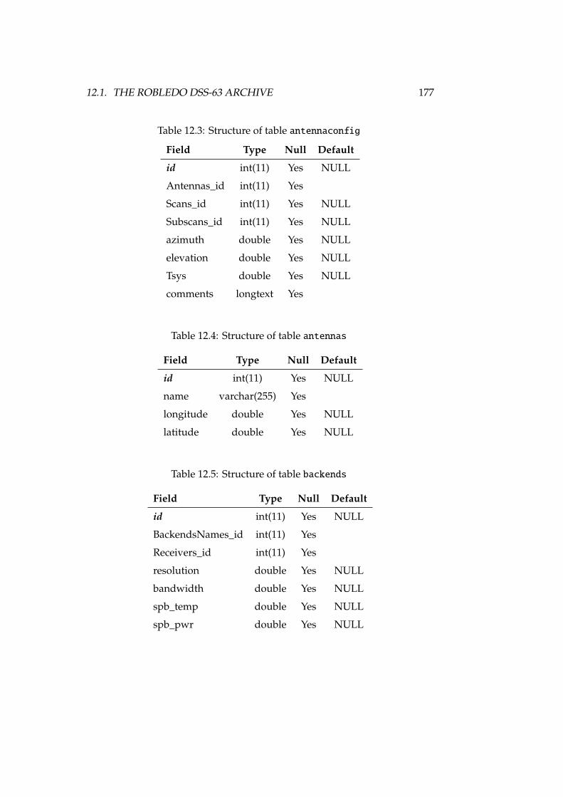
12.1. THE ROBLEDO DSS-63 ARCHIVE 177
Table 12.3: Structure of table antennaconfig
Field Type Null Default
id int(11) Yes NULL
Antennas_id int(11) Yes
Scans_id int(11) Yes NULL
Subscans_id int(11) Yes NULL
azimuth double Yes NULL
elevation double Yes NULL
Tsys double Yes NULL
comments longtext Yes
Table 12.4: Structure of table antennas
Field Type Null Default
id int(11) Yes NULL
name varchar(255) Yes
longitude double Yes NULL
latitude double Yes NULL
Table 12.5: Structure of table backends
Field Type Null Default
id int(11) Yes NULL
BackendsNames_id int(11) Yes
Receivers_id int(11) Yes
resolution double Yes NULL
bandwidth double Yes NULL
spb_temp double Yes NULL
spb_pwr double Yes NULL
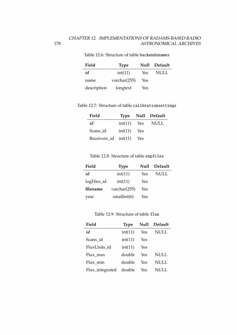
178CHAPTER 12. IMPLEMENTATIONS OF RADAMS-BASED RADIO
ASTRONOMICAL ARCHIVES
Table 12.6: Structure of table backendsnames
Field Type Null Default
id int(11) Yes NULL
name varchar(255) Yes
description longtext Yes
Table 12.7: Structure of table calibrationsettings
Field Type Null Default
id int(11) Yes NULL
Scans_id int(11) Yes
Receivers_id int(11) Yes
Table 12.8: Structure of table expfiles
Field Type Null Default
id int(11) Yes NULL
logFiles_id int(11) Yes
filename varchar(255) Yes
year smallint(6) Yes
Table 12.9: Structure of table flux
Field Type Null Default
id int(11) Yes NULL
Scans_id int(11) Yes
FluxUnits_id int(11) Yes
Flux_max double Yes NULL
Flux_min double Yes NULL
Flux_integrated double Yes NULL
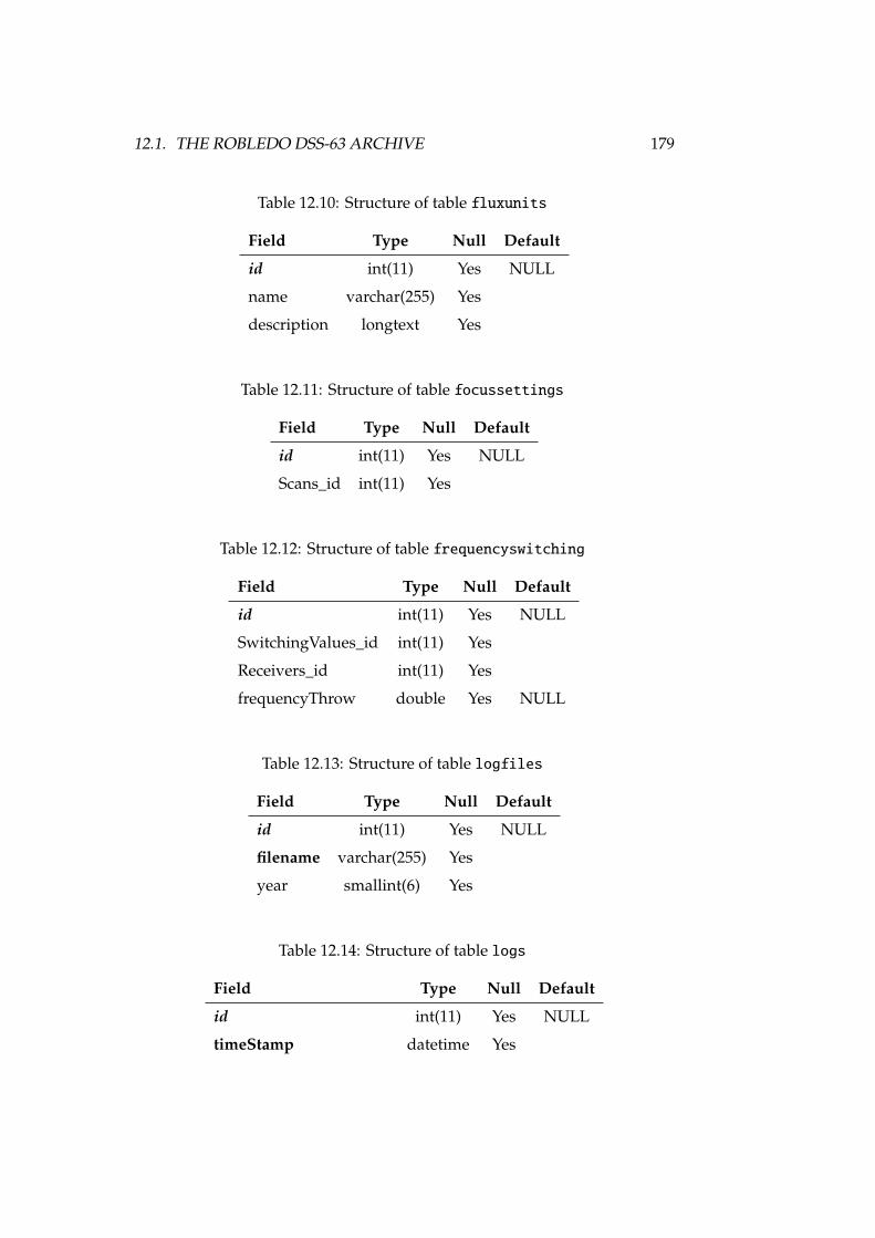
12.1. THE ROBLEDO DSS-63 ARCHIVE 179
Table 12.10: Structure of table fluxunits
Field Type Null Default
id int(11) Yes NULL
name varchar(255) Yes
description longtext Yes
Table 12.11: Structure of table focussettings
Field Type Null Default
id int(11) Yes NULL
Scans_id int(11) Yes
Table 12.12: Structure of table frequencyswitching
Field Type Null Default
id int(11) Yes NULL
SwitchingValues_id int(11) Yes
Receivers_id int(11) Yes
frequencyThrow double Yes NULL
Table 12.13: Structure of table logfiles
Field Type Null Default
id int(11) Yes NULL
filename varchar(255) Yes
year smallint(6) Yes
Table 12.14: Structure of table logs
Field Type Null Default
id int(11) Yes NULL
timeStamp datetime Yes
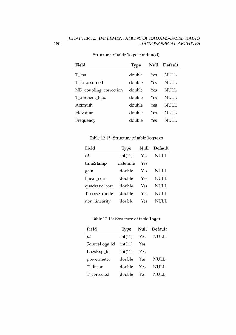
180CHAPTER 12. IMPLEMENTATIONS OF RADAMS-BASED RADIO
ASTRONOMICAL ARCHIVES
Structure of table logs (continued)
Field Type Null Default
T_lna double Yes NULL
T_fo_assumed double Yes NULL
ND_coupling_correction double Yes NULL
T_ambient_load double Yes NULL
Azimuth double Yes NULL
Elevation double Yes NULL
Frequency double Yes NULL
Table 12.15: Structure of table logsexp
Field Type Null Default
id int(11) Yes NULL
timeStamp datetime Yes
gain double Yes NULL
linear_corr double Yes NULL
quadratic_corr double Yes NULL
T_noise_diode double Yes NULL
non_linearity double Yes NULL
Table 12.16: Structure of table logst
Field Type Null Default
id int(11) Yes NULL
SourceLogs_id int(11) Yes
LogsExp_id int(11) Yes
powermeter double Yes NULL
T_linear double Yes NULL
T_corrected double Yes NULL
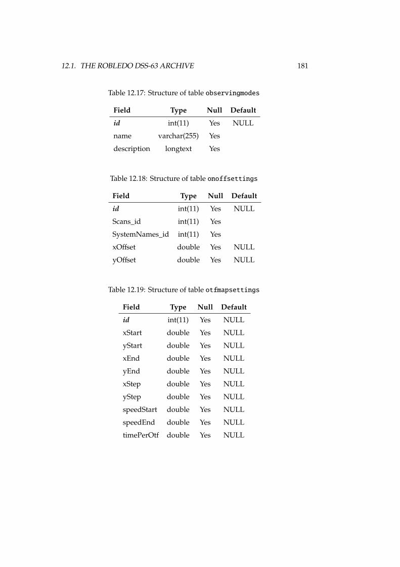
12.1. THE ROBLEDO DSS-63 ARCHIVE 181
Table 12.17: Structure of table observingmodes
Field Type Null Default
id int(11) Yes NULL
name varchar(255) Yes
description longtext Yes
Table 12.18: Structure of table onoffsettings
Field Type Null Default
id int(11) Yes NULL
Scans_id int(11) Yes
SystemNames_id int(11) Yes
xOffset double Yes NULL
yOffset double Yes NULL
Table 12.19: Structure of table otfmapsettings
Field Type Null Default
id int(11) Yes NULL
xStart double Yes NULL
yStart double Yes NULL
xEnd double Yes NULL
yEnd double Yes NULL
xStep double Yes NULL
yStep double Yes NULL
speedStart double Yes NULL
speedEnd double Yes NULL
timePerOtf double Yes NULL
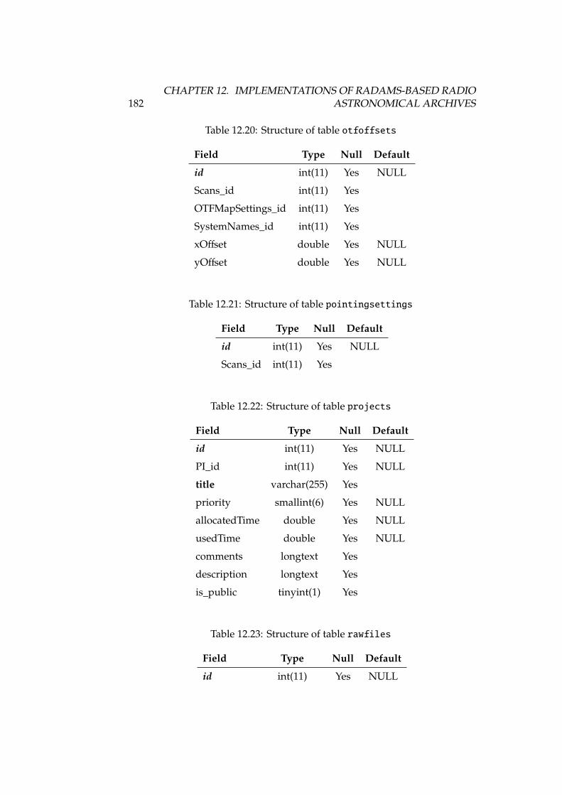
182CHAPTER 12. IMPLEMENTATIONS OF RADAMS-BASED RADIO
ASTRONOMICAL ARCHIVES
Table 12.20: Structure of table otfoffsets
Field Type Null Default
id int(11) Yes NULL
Scans_id int(11) Yes
OTFMapSettings_id int(11) Yes
SystemNames_id int(11) Yes
xOffset double Yes NULL
yOffset double Yes NULL
Table 12.21: Structure of table pointingsettings
Field Type Null Default
id int(11) Yes NULL
Scans_id int(11) Yes
Table 12.22: Structure of table projects
Field Type Null Default
id int(11) Yes NULL
PI_id int(11) Yes NULL
title varchar(255) Yes
priority smallint(6) Yes NULL
allocatedTime double Yes NULL
usedTime double Yes NULL
comments longtext Yes
description longtext Yes
is_public tinyint(1) Yes
Table 12.23: Structure of table rawfiles
Field Type Null Default
id int(11) Yes NULL
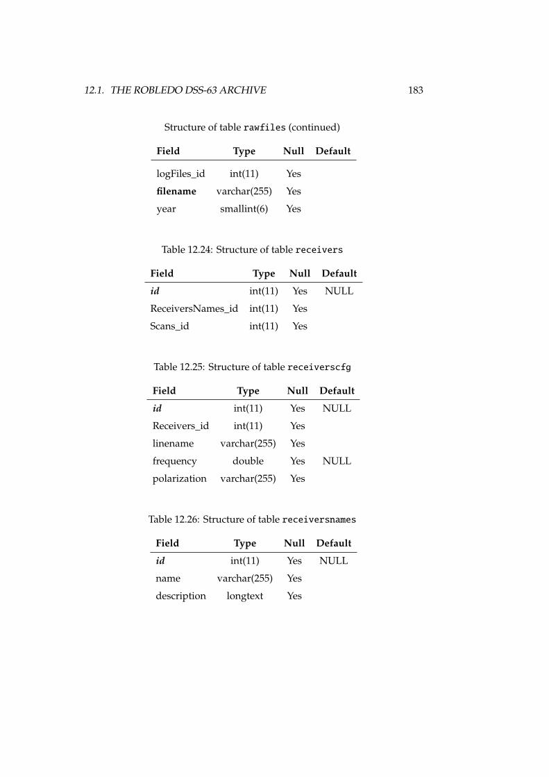
12.1. THE ROBLEDO DSS-63 ARCHIVE 183
Structure of table rawfiles (continued)
Field Type Null Default
logFiles_id int(11) Yes
filename varchar(255) Yes
year smallint(6) Yes
Table 12.24: Structure of table receivers
Field Type Null Default
id int(11) Yes NULL
ReceiversNames_id int(11) Yes
Scans_id int(11) Yes
Table 12.25: Structure of table receiverscfg
Field Type Null Default
id int(11) Yes NULL
Receivers_id int(11) Yes
linename varchar(255) Yes
frequency double Yes NULL
polarization varchar(255) Yes
Table 12.26: Structure of table receiversnames
Field Type Null Default
id int(11) Yes NULL
name varchar(255) Yes
description longtext Yes
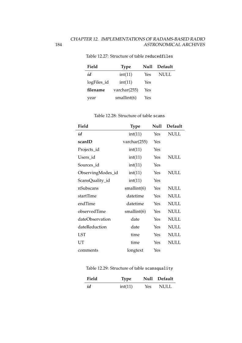
184CHAPTER 12. IMPLEMENTATIONS OF RADAMS-BASED RADIO
ASTRONOMICAL ARCHIVES
Table 12.27: Structure of table reducedfiles
Field Type Null Default
id int(11) Yes NULL
logFiles_id int(11) Yes
filename varchar(255) Yes
year smallint(6) Yes
Table 12.28: Structure of table scans
Field Type Null Default
id int(11) Yes NULL
scanID varchar(255) Yes
Projects_id int(11) Yes
Users_id int(11) Yes NULL
Sources_id int(11) Yes
ObservingModes_id int(11) Yes NULL
ScansQuality_id int(11) Yes
nSubscans smallint(6) Yes NULL
startTime datetime Yes NULL
endTime datetime Yes NULL
observedTime smallint(6) Yes NULL
dateObservation date Yes NULL
dateReduction date Yes NULL
LST time Yes NULL
UT time Yes NULL
comments longtext Yes
Table 12.29: Structure of table scansquality
Field Type Null Default
id int(11) Yes NULL
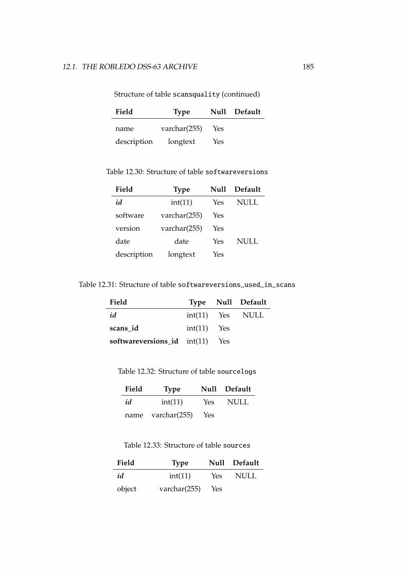
12.1. THE ROBLEDO DSS-63 ARCHIVE 185
Structure of table scansquality (continued)
Field Type Null Default
name varchar(255) Yes
description longtext Yes
Table 12.30: Structure of table softwareversions
Field Type Null Default
id int(11) Yes NULL
software varchar(255) Yes
version varchar(255) Yes
date date Yes NULL
description longtext Yes
Table 12.31: Structure of table softwareversions_used_in_scans
Field Type Null Default
id int(11) Yes NULL
scans_id int(11) Yes
softwareversions_id int(11) Yes
Table 12.32: Structure of table sourcelogs
Field Type Null Default
id int(11) Yes NULL
name varchar(255) Yes
Table 12.33: Structure of table sources
Field Type Null Default
id int(11) Yes NULL
object varchar(255) Yes
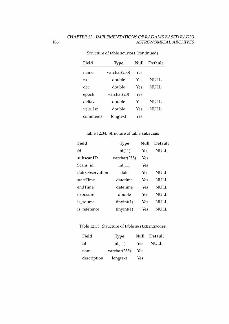
186CHAPTER 12. IMPLEMENTATIONS OF RADAMS-BASED RADIO
ASTRONOMICAL ARCHIVES
Structure of table sources (continued)
Field Type Null Default
name varchar(255) Yes
ra double Yes NULL
dec double Yes NULL
epoch varchar(20) Yes
deltav double Yes NULL
velo_lsr double Yes NULL
comments longtext Yes
Table 12.34: Structure of table subscans
Field Type Null Default
id int(11) Yes NULL
subscanID varchar(255) Yes
Scans_id int(11) Yes
dateObservation date Yes NULL
startTime datetime Yes NULL
endTime datetime Yes NULL
exposure double Yes NULL
is_source tinyint(1) Yes NULL
is_reference tinyint(1) Yes NULL
Table 12.35: Structure of table switchingmodes
Field Type Null Default
id int(11) Yes NULL
name varchar(255) Yes
description longtext Yes
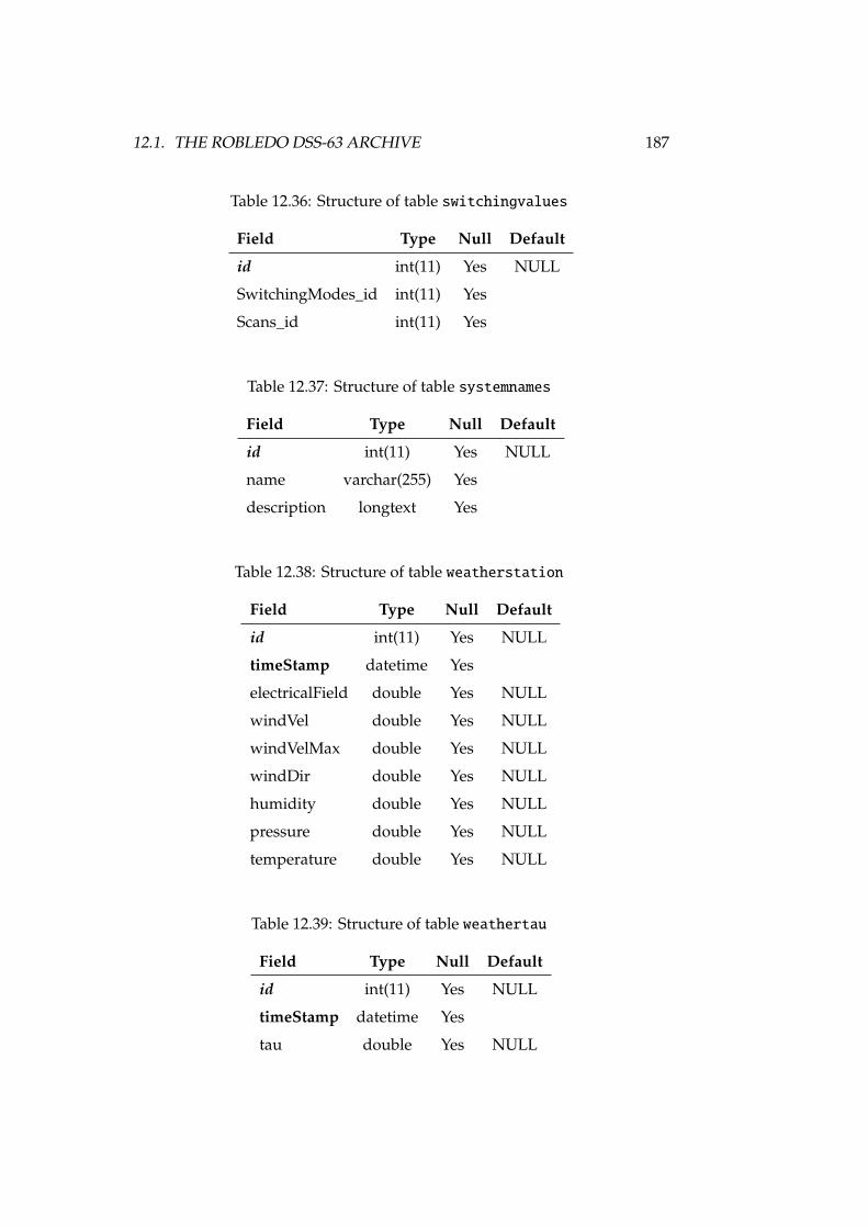
12.1. THE ROBLEDO DSS-63 ARCHIVE 187
Table 12.36: Structure of table switchingvalues
Field Type Null Default
id int(11) Yes NULL
SwitchingModes_id int(11) Yes
Scans_id int(11) Yes
Table 12.37: Structure of table systemnames
Field Type Null Default
id int(11) Yes NULL
name varchar(255) Yes
description longtext Yes
Table 12.38: Structure of table weatherstation
Field Type Null Default
id int(11) Yes NULL
timeStamp datetime Yes
electricalField double Yes NULL
windVel double Yes NULL
windVelMax double Yes NULL
windDir double Yes NULL
humidity double Yes NULL
pressure double Yes NULL
temperature double Yes NULL
Table 12.39: Structure of table weathertau
Field Type Null Default
id int(11) Yes NULL
timeStamp datetime Yes
tau double Yes NULL
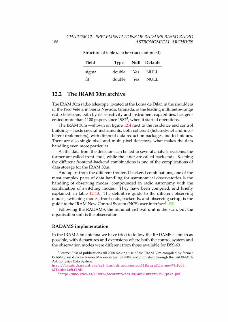
188CHAPTER 12. IMPLEMENTATIONS OF RADAMS-BASED RADIO
ASTRONOMICAL ARCHIVES
Structure of table weathertau (continued)
Field Type Null Default
sigma double Yes NULL
fit double Yes NULL
12.2 The IRAM 30m archive
The IRAM 30m radio telescope, located at the Loma de Dílar, in the shouldersof the Pico Veleta in Sierra Nevada, Granada, is the leading millimetre-rangeradio telescope, both by its sensitivity and instrument capabilities, has gen-erated more than 1100 papers since 19825, when it started operations.
The IRAM 30m —shown on figure 12.4 next to the residence and controlbuilding— hosts several instruments, both coherent (heterodyne) and inco-herent (bolometers), with different data reduction packages and techniques.There are also single-pixel and multi-pixel detectors, what makes the datahandling even more particular.
As the data from the detectors can be fed to several analysis systems, theformer are called front-ends, while the latter are called back-ends. Keepingthe different frontend-backend combinations is one of the complications ofdata storage for the IRAM 30m.
And apart from the different frontend-backend combinations, one of themost complex parts of data handling for astronomical observatories is thehandling of observing modes, compounded in radio astronomy with thecombination of switching modes. They have been compiled, and brieflyexplained, in table 12.40. The definitive guide to the different observingmodes, switching modes, front-ends, backends, and observing setup, is theguide to the IRAM New Control System (NCS) user interface6 [83].
Following the RADAMS, the minimal archival unit is the scan, but theorganisation unit is the observation.
RADAMS implementation
In the IRAM 30m antenna we have tried to follow the RADAMS as much aspossible, with departures and extensions where both the control system andthe observation modes were different from those available for DSS-63.
5Source: List of publications till 2008 making use of the IRAM 30m compiled by formerIRAM-Spain director Rainer Mauersberger till 2008, and published through the SAO/NASAAstrophysics Data System:http://adsabs.harvard.edu/cgi-bin/nph-abs_connect?library&libname=PV_Publ.&libid=45af8f27d3
6http://www.iram.es/IRAMES/documents/ncs30mPako/Current/PDF/pako.pdf
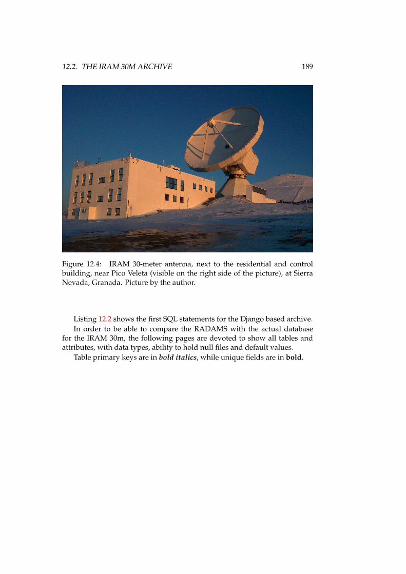
12.2. THE IRAM 30M ARCHIVE 189
Figure 12.4: IRAM 30-meter antenna, next to the residential and controlbuilding, near Pico Veleta (visible on the right side of the picture), at SierraNevada, Granada. Picture by the author.
Listing 12.2 shows the first SQL statements for the Django based archive.In order to be able to compare the RADAMS with the actual database
for the IRAM 30m, the following pages are devoted to show all tables andattributes, with data types, ability to hold null files and default values.
Table primary keys are in bold italics, while unique fields are in bold.
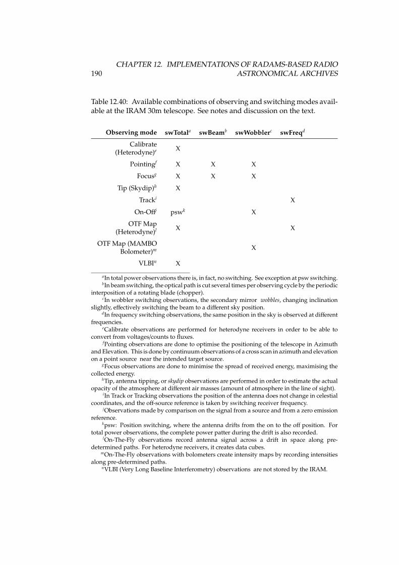
190CHAPTER 12. IMPLEMENTATIONS OF RADAMS-BASED RADIO
ASTRONOMICAL ARCHIVES
Table 12.40: Available combinations of observing and switching modes avail-able at the IRAM 30m telescope. See notes and discussion on the text.
Observing mode swTotala swBeamb swWobblerc swFreqd
Calibrate(Heterodyne)e X
Pointingf X X X
Focusg X X X
Tip (Skydip)h X
Tracki X
On-Offj pswk X
OTF Map(Heterodyne)l X X
OTF Map (MAMBOBolometer)m X
VLBIn X
aIn total power observations there is, in fact, no switching. See exception at psw switching.bIn beam switching, the optical path is cut several times per observing cycle by the periodic
interposition of a rotating blade (chopper).cIn wobbler switching observations, the secondary mirror wobbles, changing inclination
slightly, effectively switching the beam to a different sky position.dIn frequency switching observations, the same position in the sky is observed at different
frequencies.eCalibrate observations are performed for heterodyne receivers in order to be able to
convert from voltages/counts to fluxes.fPointing observations are done to optimise the positioning of the telescope in Azimuth
and Elevation. This is done by continuum observations of a cross scan in azimuth and elevationon a point source near the intended target source.
gFocus observations are done to minimise the spread of received energy, maximising thecollected energy.
hTip, antenna tipping, or skydip observations are performed in order to estimate the actualopacity of the atmosphere at different air masses (amount of atmosphere in the line of sight).
iIn Track or Tracking observations the position of the antenna does not change in celestialcoordinates, and the off-source reference is taken by switching receiver frequency.
jObservations made by comparison on the signal from a source and from a zero emissionreference.
kpsw: Position switching, where the antenna drifts from the on to the off position. Fortotal power observations, the complete power patter during the drift is also recorded.
lOn-The-Fly observations record antenna signal across a drift in space along pre-determined paths. For heterodyne receivers, it creates data cubes.
mOn-The-Fly observations with bolometers create intensity maps by recording intensitiesalong pre-determined paths.
nVLBI (Very Long Baseline Interferometry) observations are not stored by the IRAM.
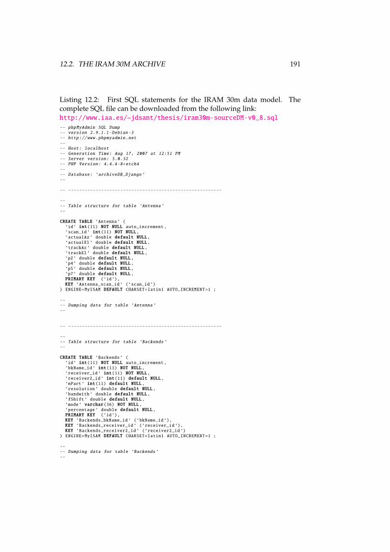
12.2. THE IRAM 30M ARCHIVE 191
Listing 12.2: First SQL statements for the IRAM 30m data model. Thecomplete SQL file can be downloaded from the following link:http://www.iaa.es/~jdsant/thesis/iram30m-sourceDM-v0_8.sql-- phpMyAdmin SQL Dump-- version 2.9.1.1-Debian -3-- http://www.phpmyadmin.net---- Host: localhost-- Generation Time: Aug 17, 2007 at 12:51 PM-- Server version: 5.0.32-- PHP Version: 4.4.4-8+etch4---- Database: ‘archiveDB_Django ‘--
-- --------------------------------------------------------
---- Table structure for table ‘Antenna‘--
CREATE TABLE ‘Antenna‘ (‘id‘ int(11) NOT NULL auto_increment ,‘scan_id‘ int(11) NOT NULL,‘actualAz ‘ double default NULL,‘actualEl ‘ double default NULL,‘trackAz‘ double default NULL,‘trackEl‘ double default NULL,‘p2‘ double default NULL,‘p4‘ double default NULL,‘p5‘ double default NULL,‘p7‘ double default NULL,PRIMARY KEY (‘id‘),KEY ‘Antenna_scan_id ‘ (‘scan_id ‘)
) ENGINE=MyISAM DEFAULT CHARSET=latin1 AUTO_INCREMENT=1 ;
---- Dumping data for table ‘Antenna‘--
-- --------------------------------------------------------
---- Table structure for table ‘Backends ‘--
CREATE TABLE ‘Backends ‘ (‘id‘ int(11) NOT NULL auto_increment ,‘bkName_id ‘ int(11) NOT NULL,‘receiver_id ‘ int(11) NOT NULL,‘receiver2_id ‘ int(11) default NULL,‘nPart‘ int(11) default NULL,‘resolution ‘ double default NULL,‘bandwith ‘ double default NULL,‘fShift‘ double default NULL,‘mode‘ varchar(36) NOT NULL,‘percentage ‘ double default NULL,PRIMARY KEY (‘id‘),KEY ‘Backends_bkName_id ‘ (‘bkName_id ‘),KEY ‘Backends_receiver_id ‘ (‘receiver_id ‘),KEY ‘Backends_receiver2_id ‘ (‘receiver2_id ‘)
) ENGINE=MyISAM DEFAULT CHARSET=latin1 AUTO_INCREMENT=1 ;
---- Dumping data for table ‘Backends ‘--
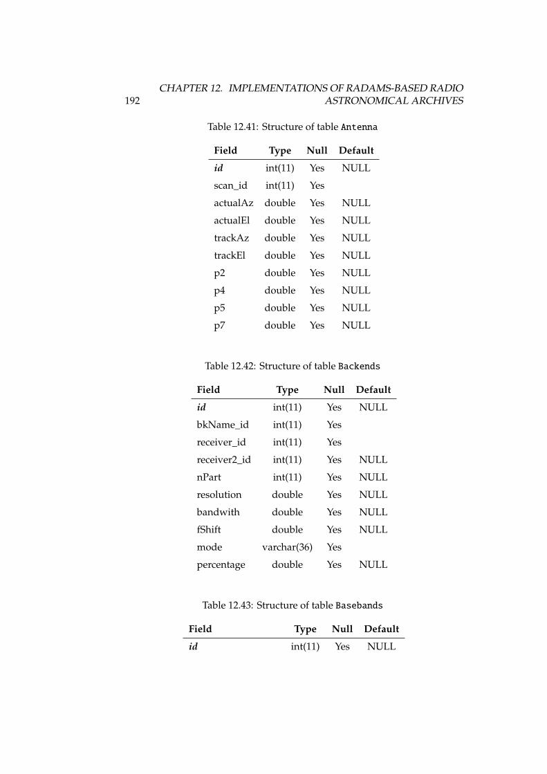
192CHAPTER 12. IMPLEMENTATIONS OF RADAMS-BASED RADIO
ASTRONOMICAL ARCHIVES
Table 12.41: Structure of table Antenna
Field Type Null Default
id int(11) Yes NULL
scan_id int(11) Yes
actualAz double Yes NULL
actualEl double Yes NULL
trackAz double Yes NULL
trackEl double Yes NULL
p2 double Yes NULL
p4 double Yes NULL
p5 double Yes NULL
p7 double Yes NULL
Table 12.42: Structure of table Backends
Field Type Null Default
id int(11) Yes NULL
bkName_id int(11) Yes
receiver_id int(11) Yes
receiver2_id int(11) Yes NULL
nPart int(11) Yes NULL
resolution double Yes NULL
bandwith double Yes NULL
fShift double Yes NULL
mode varchar(36) Yes
percentage double Yes NULL
Table 12.43: Structure of table Basebands
Field Type Null Default
id int(11) Yes NULL
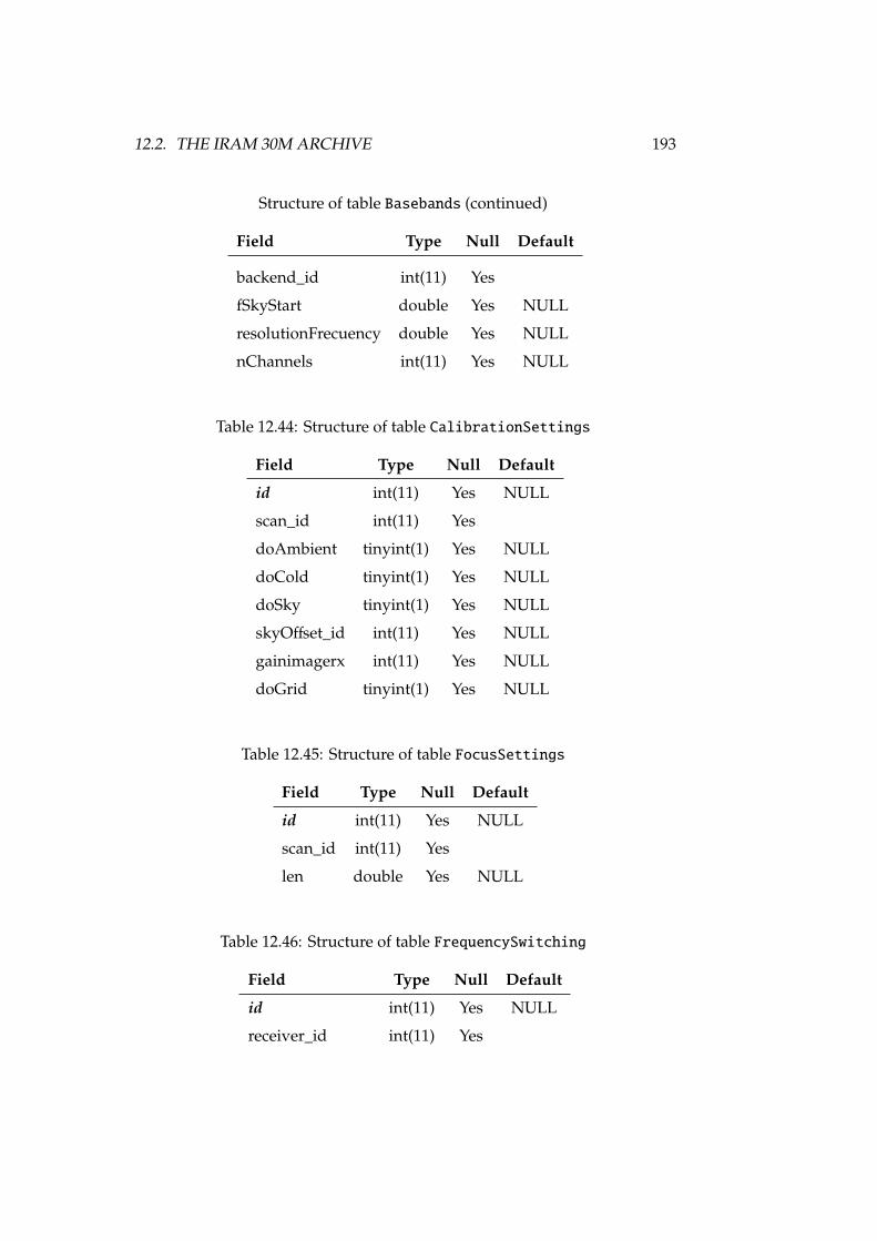
12.2. THE IRAM 30M ARCHIVE 193
Structure of table Basebands (continued)
Field Type Null Default
backend_id int(11) Yes
fSkyStart double Yes NULL
resolutionFrecuency double Yes NULL
nChannels int(11) Yes NULL
Table 12.44: Structure of table CalibrationSettings
Field Type Null Default
id int(11) Yes NULL
scan_id int(11) Yes
doAmbient tinyint(1) Yes NULL
doCold tinyint(1) Yes NULL
doSky tinyint(1) Yes NULL
skyOffset_id int(11) Yes NULL
gainimagerx int(11) Yes NULL
doGrid tinyint(1) Yes NULL
Table 12.45: Structure of table FocusSettings
Field Type Null Default
id int(11) Yes NULL
scan_id int(11) Yes
len double Yes NULL
Table 12.46: Structure of table FrequencySwitching
Field Type Null Default
id int(11) Yes NULL
receiver_id int(11) Yes
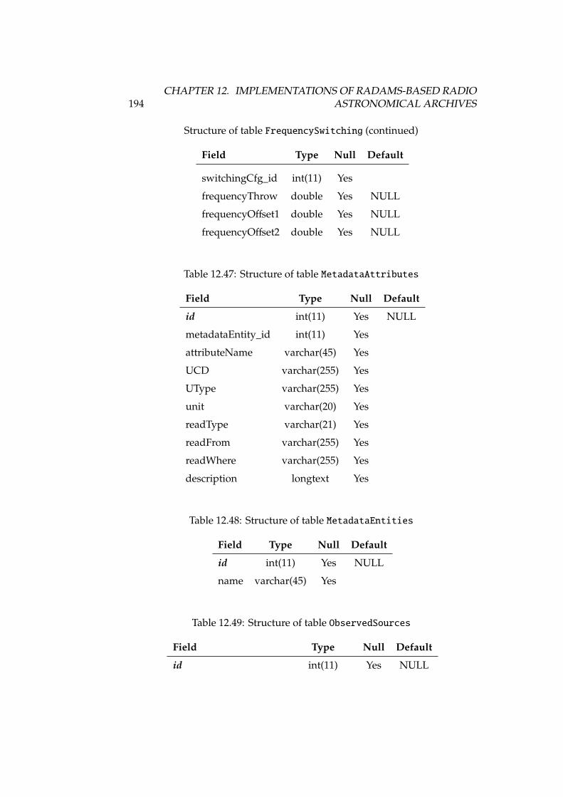
194CHAPTER 12. IMPLEMENTATIONS OF RADAMS-BASED RADIO
ASTRONOMICAL ARCHIVES
Structure of table FrequencySwitching (continued)
Field Type Null Default
switchingCfg_id int(11) Yes
frequencyThrow double Yes NULL
frequencyOffset1 double Yes NULL
frequencyOffset2 double Yes NULL
Table 12.47: Structure of table MetadataAttributes
Field Type Null Default
id int(11) Yes NULL
metadataEntity_id int(11) Yes
attributeName varchar(45) Yes
UCD varchar(255) Yes
UType varchar(255) Yes
unit varchar(20) Yes
readType varchar(21) Yes
readFrom varchar(255) Yes
readWhere varchar(255) Yes
description longtext Yes
Table 12.48: Structure of table MetadataEntities
Field Type Null Default
id int(11) Yes NULL
name varchar(45) Yes
Table 12.49: Structure of table ObservedSources
Field Type Null Default
id int(11) Yes NULL
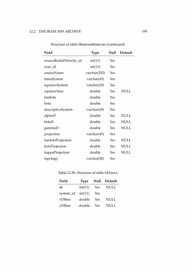
12.2. THE IRAM 30M ARCHIVE 195
Structure of table ObservedSources (continued)
Field Type Null Default
sourceRadialVelocity_id int(11) Yes
scan_id int(11) Yes
sourceName varchar(255) Yes
basisSystem varchar(45) Yes
equinoxSystem varchar(20) Yes
equinoxYear double Yes NULL
lambda double Yes
beta double Yes
descriptiveSystem varchar(45) Yes
alphaD double Yes NULL
betaD double Yes NULL
gammaD double Yes NULL
projection varchar(45) Yes
lambdaProjection double Yes NULL
betaProjection double Yes NULL
kappaProjection double Yes NULL
topology varchar(20) Yes
Table 12.50: Structure of table Offsets
Field Type Null Default
id int(11) Yes NULL
system_id int(11) Yes
xOffset double Yes NULL
yOffset double Yes NULL
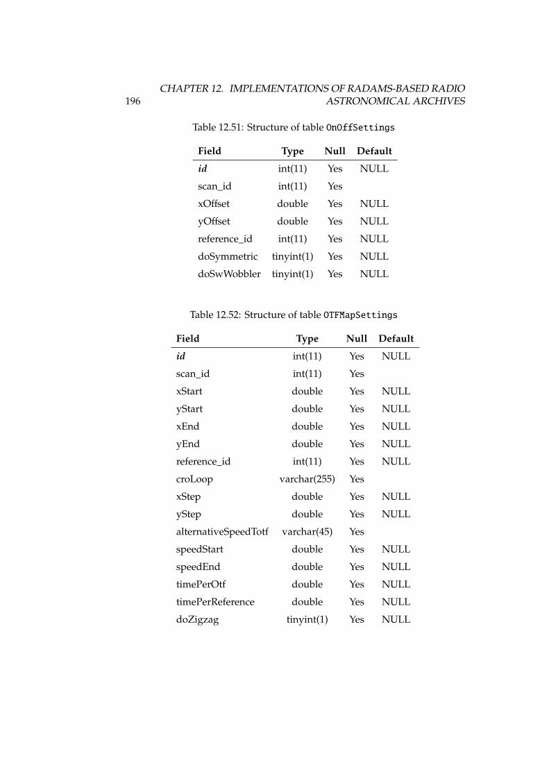
196CHAPTER 12. IMPLEMENTATIONS OF RADAMS-BASED RADIO
ASTRONOMICAL ARCHIVES
Table 12.51: Structure of table OnOffSettings
Field Type Null Default
id int(11) Yes NULL
scan_id int(11) Yes
xOffset double Yes NULL
yOffset double Yes NULL
reference_id int(11) Yes NULL
doSymmetric tinyint(1) Yes NULL
doSwWobbler tinyint(1) Yes NULL
Table 12.52: Structure of table OTFMapSettings
Field Type Null Default
id int(11) Yes NULL
scan_id int(11) Yes
xStart double Yes NULL
yStart double Yes NULL
xEnd double Yes NULL
yEnd double Yes NULL
reference_id int(11) Yes NULL
croLoop varchar(255) Yes
xStep double Yes NULL
yStep double Yes NULL
alternativeSpeedTotf varchar(45) Yes
speedStart double Yes NULL
speedEnd double Yes NULL
timePerOtf double Yes NULL
timePerReference double Yes NULL
doZigzag tinyint(1) Yes NULL

12.2. THE IRAM 30M ARCHIVE 197
Table 12.53: Structure of table PointingSettings
Field Type Null Default
id int(11) Yes NULL
scan_id int(11) Yes
len double Yes NULL
doDoubleBeam tinyint(1) Yes NULL
Table 12.54: Structure of table Pools
Field Type Null Default
id int(11) Yes NULL
name varchar(255) Yes
description varchar(255) Yes
Table 12.55: Structure of table Pools_has_Projects
Field Type Null Default
id int(11) Yes NULL
pools_id int(11) Yes
project_id int(11) Yes
Table 12.56: Structure of table PredefinedReceivers
Field Type Null Default
id int(11) Yes NULL
project_id int(11) Yes
rxName_id int(11) Yes
commentReceiver longtext Yes
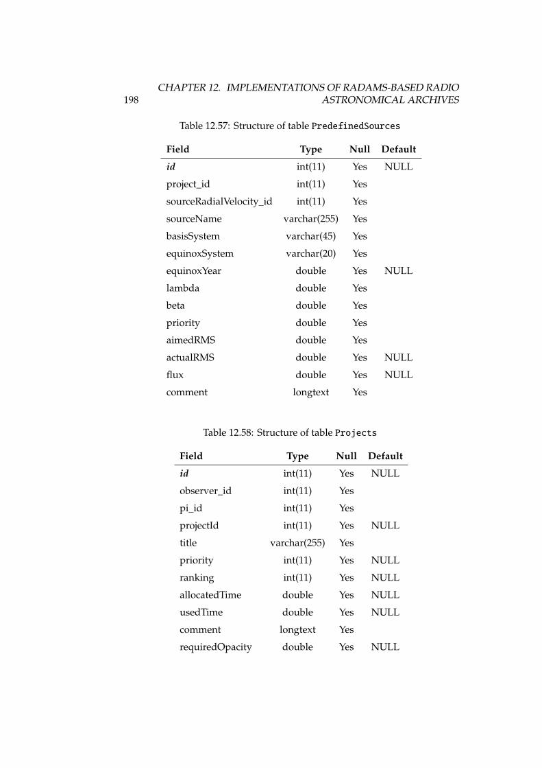
198CHAPTER 12. IMPLEMENTATIONS OF RADAMS-BASED RADIO
ASTRONOMICAL ARCHIVES
Table 12.57: Structure of table PredefinedSources
Field Type Null Default
id int(11) Yes NULL
project_id int(11) Yes
sourceRadialVelocity_id int(11) Yes
sourceName varchar(255) Yes
basisSystem varchar(45) Yes
equinoxSystem varchar(20) Yes
equinoxYear double Yes NULL
lambda double Yes
beta double Yes
priority double Yes
aimedRMS double Yes
actualRMS double Yes NULL
flux double Yes NULL
comment longtext Yes
Table 12.58: Structure of table Projects
Field Type Null Default
id int(11) Yes NULL
observer_id int(11) Yes
pi_id int(11) Yes
projectId int(11) Yes NULL
title varchar(255) Yes
priority int(11) Yes NULL
ranking int(11) Yes NULL
allocatedTime double Yes NULL
usedTime double Yes NULL
comment longtext Yes
requiredOpacity double Yes NULL
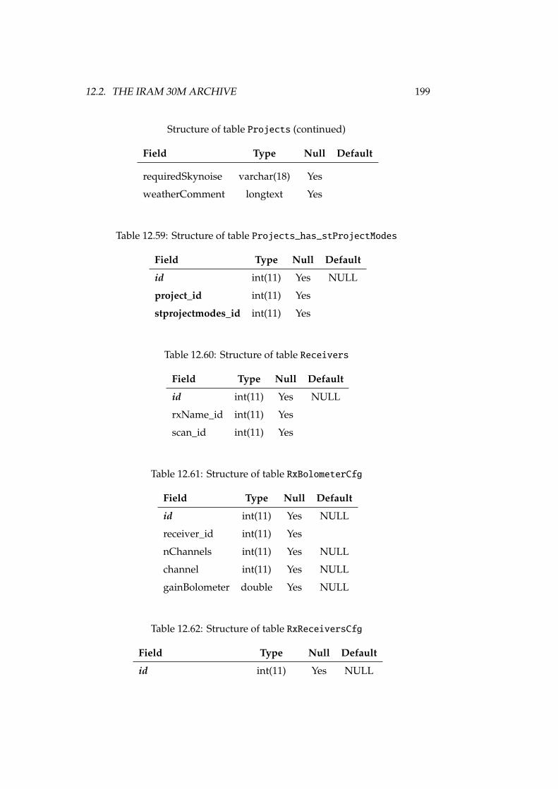
12.2. THE IRAM 30M ARCHIVE 199
Structure of table Projects (continued)
Field Type Null Default
requiredSkynoise varchar(18) Yes
weatherComment longtext Yes
Table 12.59: Structure of table Projects_has_stProjectModes
Field Type Null Default
id int(11) Yes NULL
project_id int(11) Yes
stprojectmodes_id int(11) Yes
Table 12.60: Structure of table Receivers
Field Type Null Default
id int(11) Yes NULL
rxName_id int(11) Yes
scan_id int(11) Yes
Table 12.61: Structure of table RxBolometerCfg
Field Type Null Default
id int(11) Yes NULL
receiver_id int(11) Yes
nChannels int(11) Yes NULL
channel int(11) Yes NULL
gainBolometer double Yes NULL
Table 12.62: Structure of table RxReceiversCfg
Field Type Null Default
id int(11) Yes NULL
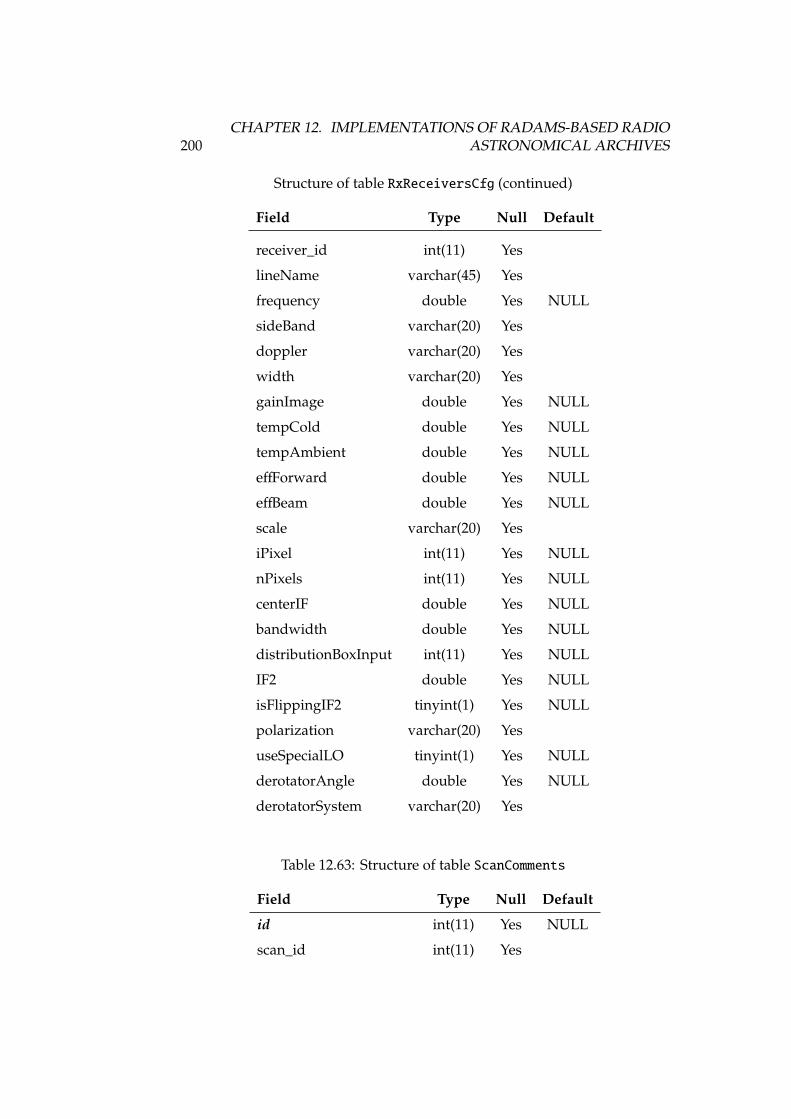
200CHAPTER 12. IMPLEMENTATIONS OF RADAMS-BASED RADIO
ASTRONOMICAL ARCHIVES
Structure of table RxReceiversCfg (continued)
Field Type Null Default
receiver_id int(11) Yes
lineName varchar(45) Yes
frequency double Yes NULL
sideBand varchar(20) Yes
doppler varchar(20) Yes
width varchar(20) Yes
gainImage double Yes NULL
tempCold double Yes NULL
tempAmbient double Yes NULL
effForward double Yes NULL
effBeam double Yes NULL
scale varchar(20) Yes
iPixel int(11) Yes NULL
nPixels int(11) Yes NULL
centerIF double Yes NULL
bandwidth double Yes NULL
distributionBoxInput int(11) Yes NULL
IF2 double Yes NULL
isFlippingIF2 tinyint(1) Yes NULL
polarization varchar(20) Yes
useSpecialLO tinyint(1) Yes NULL
derotatorAngle double Yes NULL
derotatorSystem varchar(20) Yes
Table 12.63: Structure of table ScanComments
Field Type Null Default
id int(11) Yes NULL
scan_id int(11) Yes
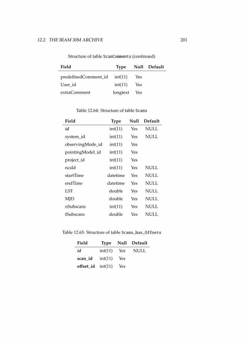
12.2. THE IRAM 30M ARCHIVE 201
Structure of table ScanComments (continued)
Field Type Null Default
predefinedComment_id int(11) Yes
User_id int(11) Yes
extraComment longtext Yes
Table 12.64: Structure of table Scans
Field Type Null Default
id int(11) Yes NULL
system_id int(11) Yes NULL
observingMode_id int(11) Yes
pointingModel_id int(11) Yes
project_id int(11) Yes
ncsId int(11) Yes NULL
startTime datetime Yes NULL
endTime datetime Yes NULL
LST double Yes NULL
MJD double Yes NULL
nSubscans int(11) Yes NULL
tSubscans double Yes NULL
Table 12.65: Structure of table Scans_has_Offsets
Field Type Null Default
id int(11) Yes NULL
scan_id int(11) Yes
offset_id int(11) Yes
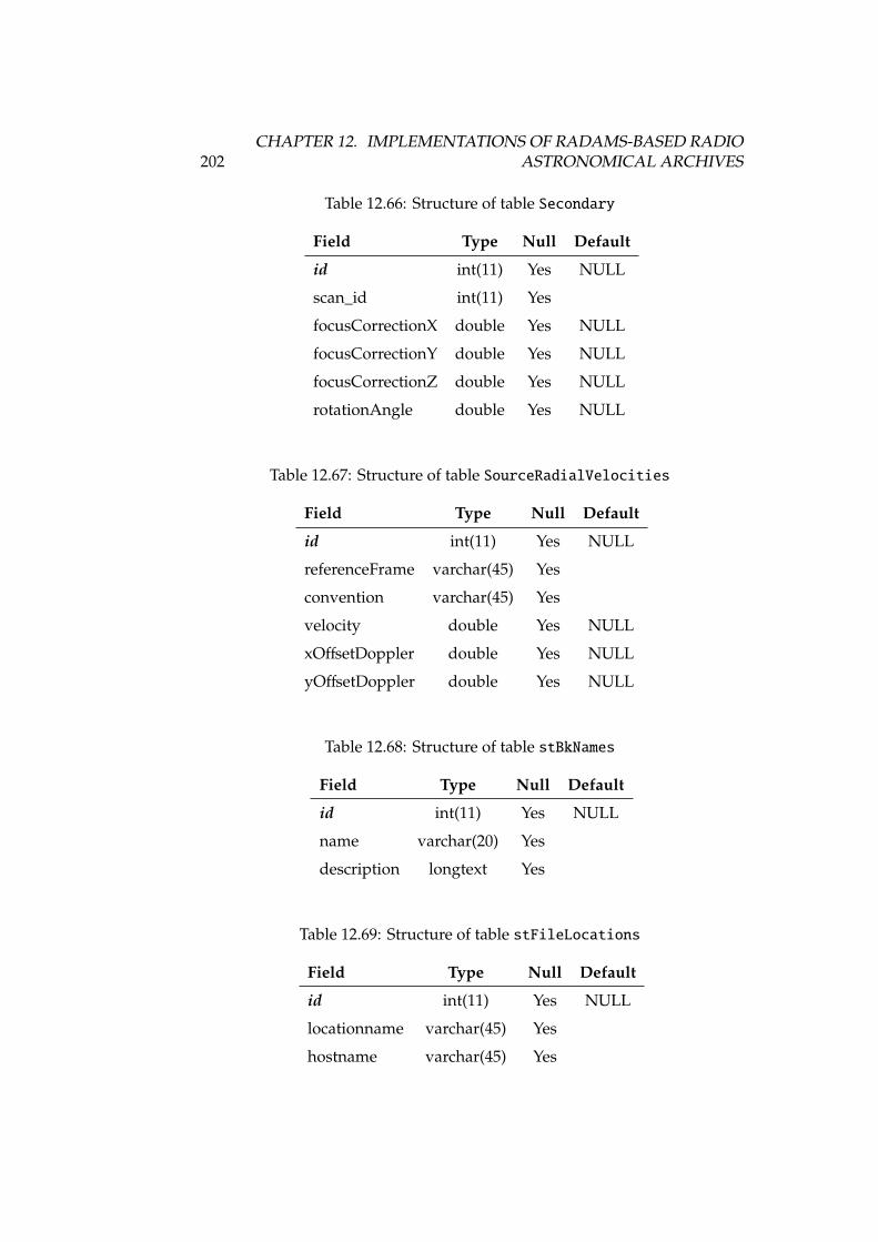
202CHAPTER 12. IMPLEMENTATIONS OF RADAMS-BASED RADIO
ASTRONOMICAL ARCHIVES
Table 12.66: Structure of table Secondary
Field Type Null Default
id int(11) Yes NULL
scan_id int(11) Yes
focusCorrectionX double Yes NULL
focusCorrectionY double Yes NULL
focusCorrectionZ double Yes NULL
rotationAngle double Yes NULL
Table 12.67: Structure of table SourceRadialVelocities
Field Type Null Default
id int(11) Yes NULL
referenceFrame varchar(45) Yes
convention varchar(45) Yes
velocity double Yes NULL
xOffsetDoppler double Yes NULL
yOffsetDoppler double Yes NULL
Table 12.68: Structure of table stBkNames
Field Type Null Default
id int(11) Yes NULL
name varchar(20) Yes
description longtext Yes
Table 12.69: Structure of table stFileLocations
Field Type Null Default
id int(11) Yes NULL
locationname varchar(45) Yes
hostname varchar(45) Yes
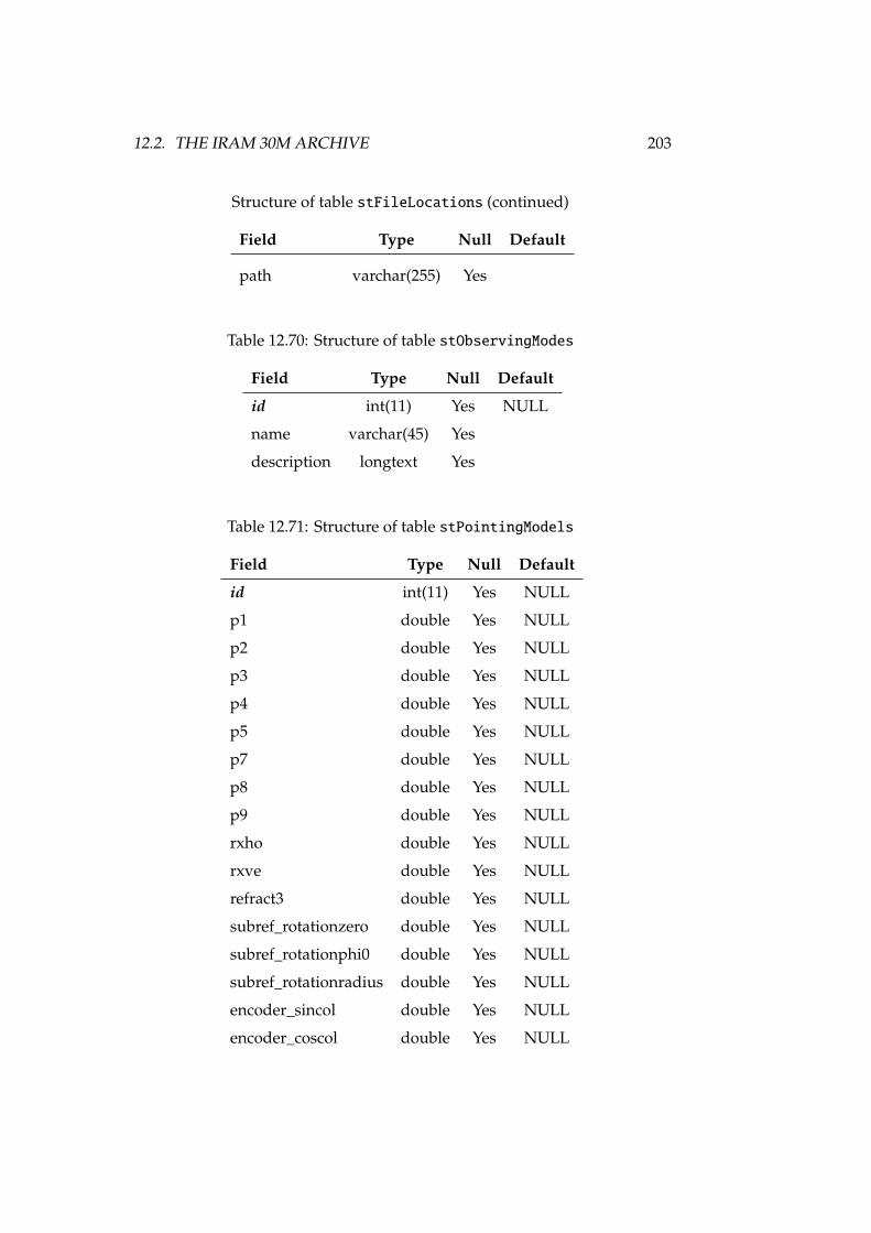
12.2. THE IRAM 30M ARCHIVE 203
Structure of table stFileLocations (continued)
Field Type Null Default
path varchar(255) Yes
Table 12.70: Structure of table stObservingModes
Field Type Null Default
id int(11) Yes NULL
name varchar(45) Yes
description longtext Yes
Table 12.71: Structure of table stPointingModels
Field Type Null Default
id int(11) Yes NULL
p1 double Yes NULL
p2 double Yes NULL
p3 double Yes NULL
p4 double Yes NULL
p5 double Yes NULL
p7 double Yes NULL
p8 double Yes NULL
p9 double Yes NULL
rxho double Yes NULL
rxve double Yes NULL
refract3 double Yes NULL
subref_rotationzero double Yes NULL
subref_rotationphi0 double Yes NULL
subref_rotationradius double Yes NULL
encoder_sincol double Yes NULL
encoder_coscol double Yes NULL
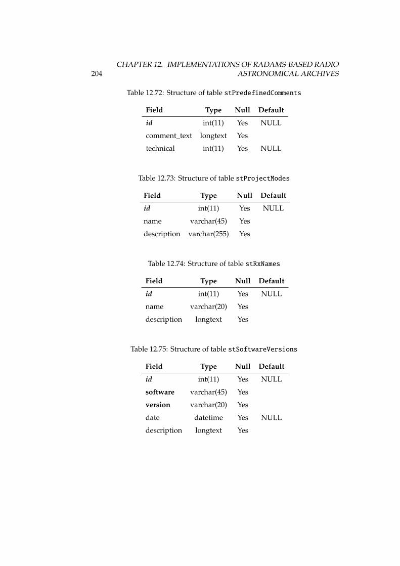
204CHAPTER 12. IMPLEMENTATIONS OF RADAMS-BASED RADIO
ASTRONOMICAL ARCHIVES
Table 12.72: Structure of table stPredefinedComments
Field Type Null Default
id int(11) Yes NULL
comment_text longtext Yes
technical int(11) Yes NULL
Table 12.73: Structure of table stProjectModes
Field Type Null Default
id int(11) Yes NULL
name varchar(45) Yes
description varchar(255) Yes
Table 12.74: Structure of table stRxNames
Field Type Null Default
id int(11) Yes NULL
name varchar(20) Yes
description longtext Yes
Table 12.75: Structure of table stSoftwareVersions
Field Type Null Default
id int(11) Yes NULL
software varchar(45) Yes
version varchar(20) Yes
date datetime Yes NULL
description longtext Yes
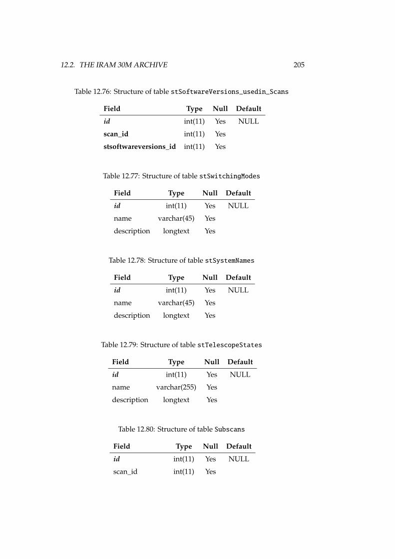
12.2. THE IRAM 30M ARCHIVE 205
Table 12.76: Structure of table stSoftwareVersions_usedin_Scans
Field Type Null Default
id int(11) Yes NULL
scan_id int(11) Yes
stsoftwareversions_id int(11) Yes
Table 12.77: Structure of table stSwitchingModes
Field Type Null Default
id int(11) Yes NULL
name varchar(45) Yes
description longtext Yes
Table 12.78: Structure of table stSystemNames
Field Type Null Default
id int(11) Yes NULL
name varchar(45) Yes
description longtext Yes
Table 12.79: Structure of table stTelescopeStates
Field Type Null Default
id int(11) Yes NULL
name varchar(255) Yes
description longtext Yes
Table 12.80: Structure of table Subscans
Field Type Null Default
id int(11) Yes NULL
scan_id int(11) Yes
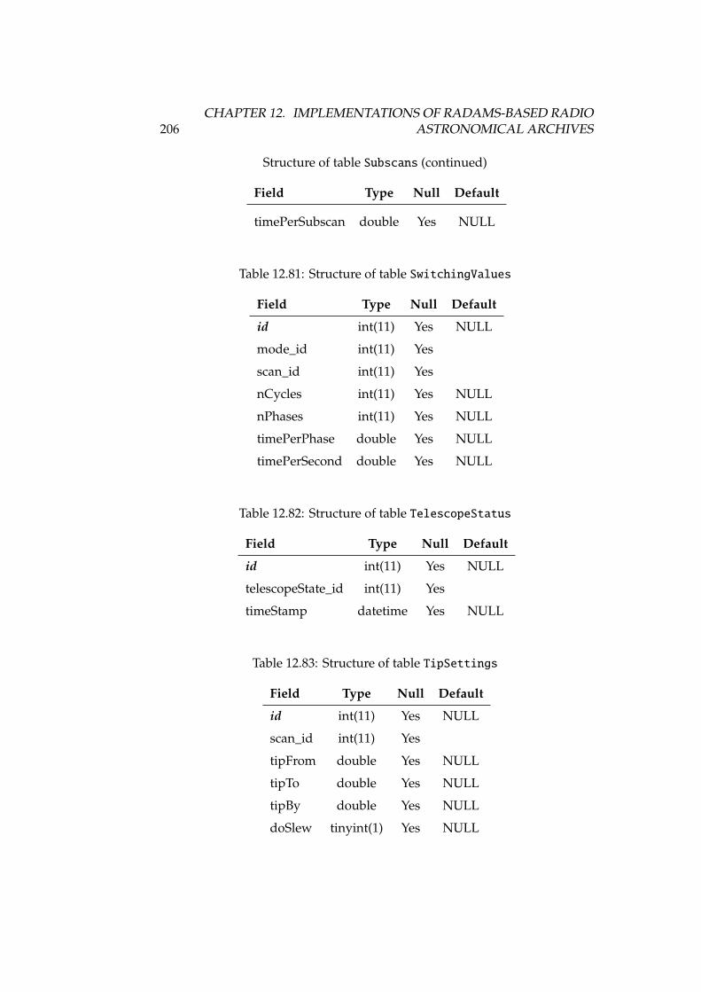
206CHAPTER 12. IMPLEMENTATIONS OF RADAMS-BASED RADIO
ASTRONOMICAL ARCHIVES
Structure of table Subscans (continued)
Field Type Null Default
timePerSubscan double Yes NULL
Table 12.81: Structure of table SwitchingValues
Field Type Null Default
id int(11) Yes NULL
mode_id int(11) Yes
scan_id int(11) Yes
nCycles int(11) Yes NULL
nPhases int(11) Yes NULL
timePerPhase double Yes NULL
timePerSecond double Yes NULL
Table 12.82: Structure of table TelescopeStatus
Field Type Null Default
id int(11) Yes NULL
telescopeState_id int(11) Yes
timeStamp datetime Yes NULL
Table 12.83: Structure of table TipSettings
Field Type Null Default
id int(11) Yes NULL
scan_id int(11) Yes
tipFrom double Yes NULL
tipTo double Yes NULL
tipBy double Yes NULL
doSlew tinyint(1) Yes NULL
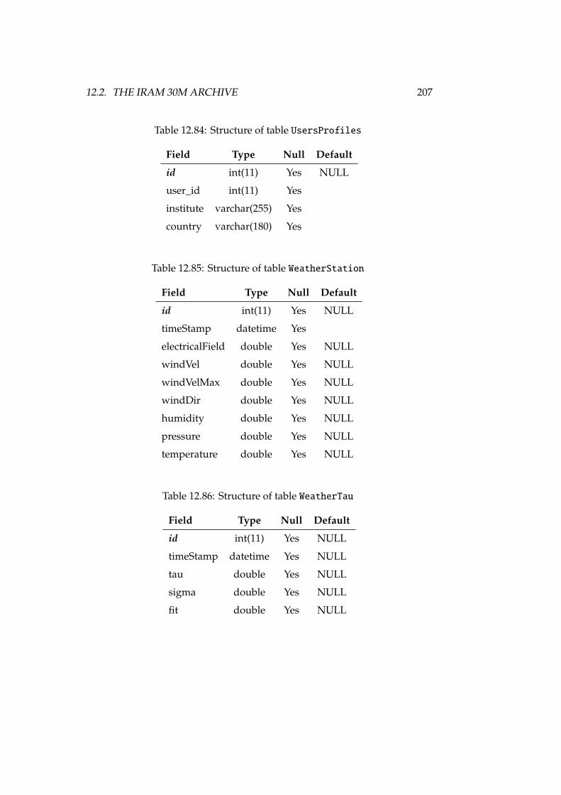
12.2. THE IRAM 30M ARCHIVE 207
Table 12.84: Structure of table UsersProfiles
Field Type Null Default
id int(11) Yes NULL
user_id int(11) Yes
institute varchar(255) Yes
country varchar(180) Yes
Table 12.85: Structure of table WeatherStation
Field Type Null Default
id int(11) Yes NULL
timeStamp datetime Yes
electricalField double Yes NULL
windVel double Yes NULL
windVelMax double Yes NULL
windDir double Yes NULL
humidity double Yes NULL
pressure double Yes NULL
temperature double Yes NULL
Table 12.86: Structure of table WeatherTau
Field Type Null Default
id int(11) Yes NULL
timeStamp datetime Yes NULL
tau double Yes NULL
sigma double Yes NULL
fit double Yes NULL
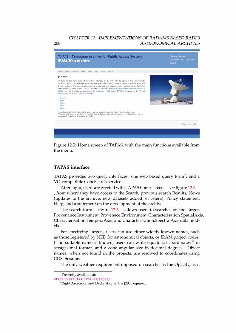
208CHAPTER 12. IMPLEMENTATIONS OF RADAMS-BASED RADIO
ASTRONOMICAL ARCHIVES
IRAM - IAA - CSIC
Home Search Results News Policy Help About Admin
HomeWelcome to the home page of the archive interface of the IRAM-30m telescope in the Sierra Nevada(Granada, Spain). The Telescope Access for Public Archive System (TAPAS) is meant to provide public andprivate access to the observation headers (projects, sources, frequency, etc) recorded at the IRAM-30mtelescope and to public projects. It is a collaboration between the Instituto de Radioastronomía Millimétrica(IRAM) and the Instituto de Astrofísica de Andalucía - CSIC (IAA). TAPAS is included in the VirtualObservatory and is built to be VO-compliant.
SearchNewsPolicyHelpAbout
If you have used TAPAS facilities for your research, please include the following acknowledgment: "This research used the facilities of the Instituto de Radioastronomía Millimétrica in collaboration with theInstituto de Astrofísica de Andalucía - CSIC."
TAPAS - Telescope Archive for Public Access SystemIRAM 30m Archive
Welcome Stephane
Last logged: Sun, 29 Mar 2009
Logout
Figure 12.5: Home screen of TAPAS, with the main functions available fromthe menu.
TAPAS interface
TAPAS provides two query interfaces: one web based query form7, and aVO-compatible ConeSearch service.
After login, users are greeted with TAPAS home screen —see figure 12.5—, from where they have access to the Search, previous search Results, News(updates to the archive, new datasets added, et cetera), Policy statement,Help, and a statement on the development of the archive.
The search form —figure 12.6— allows users to searches on the Target,Provenance.Instrument, Provenace.Environment, Characterisation.SpatialAxis,Characterisation.TemporaAxis, and Characterisation.SpectralAxis data mod-els.
For specifying Targets, users can use either widely known names, suchas those registered by NED for astronomical objects, or IRAM project codes.If no suitable name is known, users can write equatorial coordinates 8 insexagesimal format, and a cone angular size in decimal degrees. Objectnames, when not found in the projects, are resolved to coordinates usingCDS’ Sesame.
The only weather requirement imposed on searches is the Opacity, as it
7Presently available at:https://mrt-lx3.iram.es/tapas/
8Right Ascension and Declination in the J2000 equinox
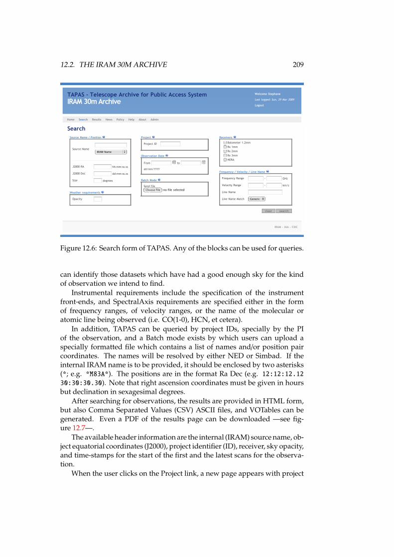
12.2. THE IRAM 30M ARCHIVE 209
SearchSource Name / Position
Source NameIRAM Name
J2000 RA hh:mm:ss.ss
J2000 Dec dd:mm:ss.ss
Size degrees
Weather requirements
Opacity
Project
Project ID
Observation Date
From to
dd/mm/YYYY
Batch Mode
Send fileno file selectedChoose File
Receivers
Bolometer 1.2mm Rx 1mm Rx 2mm Rx 3mm HERA
Frequency / Velocity / Line Name
Frequency Range - GHz
Velocity Range - km/s
Line Name
Line Name Match Generic
clear search
IRAM - IAA - CSIC
Home Search Results News Policy Help About Admin
TAPAS - Telescope Archive for Public Access SystemIRAM 30m Archive
Welcome Stephane
Last logged: Sun, 29 Mar 2009
Logout
Figure 12.6: Search form of TAPAS. Any of the blocks can be used for queries.
can identify those datasets which have had a good enough sky for the kindof observation we intend to find.
Instrumental requirements include the specification of the instrumentfront-ends, and SpectralAxis requirements are specified either in the formof frequency ranges, of velocity ranges, or the name of the molecular oratomic line being observed (i.e. CO(1-0), HCN, et cetera).
In addition, TAPAS can be queried by project IDs, specially by the PIof the observation, and a Batch mode exists by which users can upload aspecially formatted file which contains a list of names and/or position paircoordinates. The names will be resolved by either NED or Simbad. If theinternal IRAM name is to be provided, it should be enclosed by two asterisks(*; e.g. *M83A*). The positions are in the format Ra Dec (e.g. 12:12:12.1230:30:30.30). Note that right ascension coordinates must be given in hoursbut declination in sexagesimal degrees.
After searching for observations, the results are provided in HTML form,but also Comma Separated Values (CSV) ASCII files, and VOTables can begenerated. Even a PDF of the results page can be downloaded —see fig-ure 12.7—.
The available header information are the internal (IRAM) source name, ob-ject equatorial coordinates (J2000), project identifier (ID), receiver, sky opacity,and time-stamps for the start of the first and the latest scans for the observa-tion.
When the user clicks on the Project link, a new page appears with project
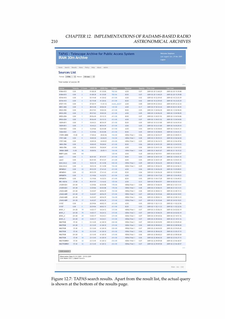
210CHAPTER 12. IMPLEMENTATIONS OF RADAMS-BASED RADIO
ASTRONOMICAL ARCHIVES
Sources ListFormat HTML Return 50 rows
Total number of sources: 85
>>>
Source Velocity # Scans J2000 RA J2000 Dec. Project Receiver Opacity First Scan Last Scan
0106+013 0.00 3 01:08:38 01:35:00 T02-06 A230 0.07 2009-02-20 13:40:29 2009-02-20 15:39:08
0106+013 0.00 3 01:08:38 01:35:00 T02-06 B230 0.07 2009-02-20 13:40:29 2009-02-20 15:39:08
0316+413 0.00 4 03:19:48 41:30:42 d13-08 A230 0.02 2009-02-10 22:59:45 2009-02-10 23:25:39
0316+413 0.00 4 03:19:48 41:30:42 d13-08 B230 0.02 2009-02-10 22:59:45 2009-02-10 23:25:39
0727-115 0.00 1 07:30:19 -11:41:12 monit_oh231 A230 0.00 2009-03-09 22:30:22 2009-03-09 22:32:34
0851+202 0.00 3 08:54:48 20:06:30 125-08 A230 0.17 2009-02-27 02:32:44 2009-03-02 01:30:45
0923+392 0.00 1 09:27:03 39:02:20 d13-08 B230 0.05 2009-02-13 04:56:30 2009-02-13 04:58:45
0923+392 0.00 1 09:27:03 39:02:20 d13-08 A230 0.05 2009-02-13 04:56:30 2009-02-13 04:58:45
0953+254 0.00 1 09:56:49 25:15:15 d13-08 B230 0.07 2009-02-13 04:51:52 2009-02-13 04:54:06
0953+254 0.00 1 09:56:49 25:15:15 d13-08 A230 0.07 2009-02-13 04:51:52 2009-02-13 04:54:06
1039+811 0.00 7 10:44:23 80:54:39 d13-08 B230 0.05 2009-02-10 23:31:00 2009-02-16 04:29:34
1039+811 0.00 7 10:44:23 80:54:39 d13-08 A230 0.05 2009-02-10 23:31:00 2009-02-16 04:29:34
1226+023 0.00 3 12:29:06 02:03:08 d13-08 A230 0.05 2009-02-12 03:58:45 2009-02-12 04:41:31
1226+023 0.00 3 12:29:06 02:03:08 d13-08 B230 0.05 2009-02-12 03:58:45 2009-02-12 04:41:31
17455-2800 -15.00 21 17:48:42 -28:02:06 154-08 HERA1 Pixel 1 0.06 2009-02-23 06:54:37 2009-02-23 08:05:31
1757-240 0.00 9 18:00:30 -24:04:01 154-08 HERA1 Pixel 1 0.08 2009-02-21 05:55:33 2009-02-23 06:56:50
1757-240 0.00 1 18:00:30 -24:04:01 d16-08 HERA1 Pixel 1 0.05 2009-02-23 06:34:15 2009-02-23 06:49:56
1803+784 0.00 1 18:00:45 78:28:04 d13-08 B230 0.06 2009-02-12 04:51:39 2009-02-12 04:53:53
1803+784 0.00 1 18:00:45 78:28:04 d13-08 A230 0.06 2009-02-12 04:51:39 2009-02-12 04:53:53
18060-2005 13.00 58 18:08:56 -20:05:11 154-08 HERA1 Pixel 1 0.08 2009-02-21 06:01:07 2009-02-21 10:15:32
BODY Lulin 0.00 84 125-08 A230 0.20 2009-02-27 00:19:51 2009-03-02 03:02:47
core1 0.00 3 02:01:05 87:41:57 d13-08 B230 0.05 2009-02-12 04:51:39 2009-02-12 05:01:35
core1 0.00 3 02:01:05 87:41:57 d13-08 A230 0.05 2009-02-12 04:51:39 2009-02-12 05:01:35
G34.3+0.2 0.00 1 18:53:18 01:14:58 030-08 HERA1 Pixel 1 0.09 2009-02-21 05:26:35 2009-02-21 05:46:11
G34.3+0.2 0.00 6 18:53:18 01:14:58 154-08 HERA1 Pixel 1 0.09 2009-02-21 05:26:35 2009-02-22 04:56:31
HIP48541 0.00 22 09:53:59 27:41:43 d13-08 A230 0.06 2009-02-13 04:56:30 2009-02-15 05:00:01
HIP48541 0.00 22 09:53:59 27:41:43 d13-08 B230 0.06 2009-02-13 04:56:30 2009-02-15 05:00:01
HIP60074 0.00 9 12:19:06 16:32:53 d13-08 A230 0.05 2009-02-13 04:17:28 2009-02-13 04:49:23
HIP60074 0.00 9 12:19:06 16:32:53 d13-08 B230 0.05 2009-02-13 04:17:28 2009-02-13 04:49:23
IRC+10216 -27.00 4 09:47:57 13:16:42 125-08 A230 0.23 2009-02-27 00:42:57 2009-03-02 02:14:31
J1229+021 241.00 1 12:29:06 02:03:08 178-08 HERA2 Pixel 1 0.08 2009-02-21 03:06:35 2009-02-21 03:13:31
J1229+021 241.00 1 12:29:06 02:03:08 178-08 HERA1 Pixel 1 0.08 2009-02-21 03:06:35 2009-02-21 03:13:31
J1642+689 241.00 1 16:42:07 68:56:39 154-08 HERA2 Pixel 1 0.06 2009-02-23 08:02:14 2009-02-23 08:15:12
J1642+689 241.00 17 16:42:07 68:56:39 215-08 HERA1 Pixel 1 0.07 2009-02-21 03:35:46 2009-02-24 02:10:01
J1642+689 241.00 1 16:42:07 68:56:39 154-08 HERA1 Pixel 1 0.06 2009-02-23 08:02:14 2009-02-23 08:15:12
J1642+689 241.00 17 16:42:07 68:56:39 215-08 HERA2 Pixel 1 0.07 2009-02-21 03:35:46 2009-02-24 02:10:01
l1157 0.00 3 20:39:06 68:02:15 d13-08 A230 0.05 2009-02-11 02:11:33 2009-02-11 02:22:56
l1157 0.00 3 20:39:06 68:02:15 d13-08 B230 0.05 2009-02-11 02:11:33 2009-02-11 02:22:56
M101_1 241.00 79 14:03:17 54:24:12 215-08 HERA2 Pixel 1 0.07 2009-02-21 03:06:35 2009-02-24 02:02:19
M101_1 241.00 79 14:03:17 54:24:12 215-08 HERA1 Pixel 1 0.07 2009-02-21 03:06:35 2009-02-24 02:02:19
M101_3 241.00 29 14:03:17 54:24:21 215-08 HERA1 Pixel 1 0.07 2009-02-23 09:30:36 2009-02-23 10:51:16
M101_3 241.00 29 14:03:17 54:24:21 215-08 HERA2 Pixel 1 0.07 2009-02-23 09:30:36 2009-02-23 10:51:16
NGC7538 -57.40 1 23:13:45 61:28:10 030-08 HERA1 Pixel 1 0.07 2009-02-23 04:54:59 2009-02-23 05:05:42
NGC7538 241.00 3 23:13:45 61:28:10 215-08 HERA1 Pixel 1 0.06 2009-02-23 08:40:23 2009-02-23 08:50:28
NGC7538 -57.40 1 23:13:45 61:28:10 030-08 HERA2 Pixel 1 0.07 2009-02-23 04:54:59 2009-02-23 05:05:42
NGC7538 -57.40 10 23:13:45 61:28:10 d16-08 HERA1 Pixel 1 0.06 2009-02-22 08:46:30 2009-02-23 05:37:15
NGC7538 241.00 3 23:13:45 61:28:10 215-08 HERA2 Pixel 1 0.06 2009-02-23 08:40:23 2009-02-23 08:50:28
NGC7538 -57.40 10 23:13:45 61:28:10 d16-08 HERA2 Pixel 1 0.06 2009-02-22 08:46:30 2009-02-23 05:37:15
NGC7538IRS1 -57.40 32 23:13:45 61:28:12 d16-08 HERA1 Pixel 1 0.07 2009-02-22 09:09:58 2009-02-23 06:40:57
NGC7538IRS1 -57.40 32 23:13:45 61:28:12 d16-08 HERA2 Pixel 1 0.07 2009-02-22 09:09:58 2009-02-23 06:40:57
>>>
Edit search
Observation Date 01/01/2009 - 29/03/2009Line Name CO(2-1) Match Generic
IRAM - IAA - CSIC
Home Search Results News Policy Help About Admin
TAPAS - Telescope Archive for Public Access SystemIRAM 30m Archive
Welcome Stephane
Last logged: Sun, 29 Mar 2009
Logout
Figure 12.7: TAPAS search results. Apart from the result list, the actual queryis shown at the bottom of the results page.
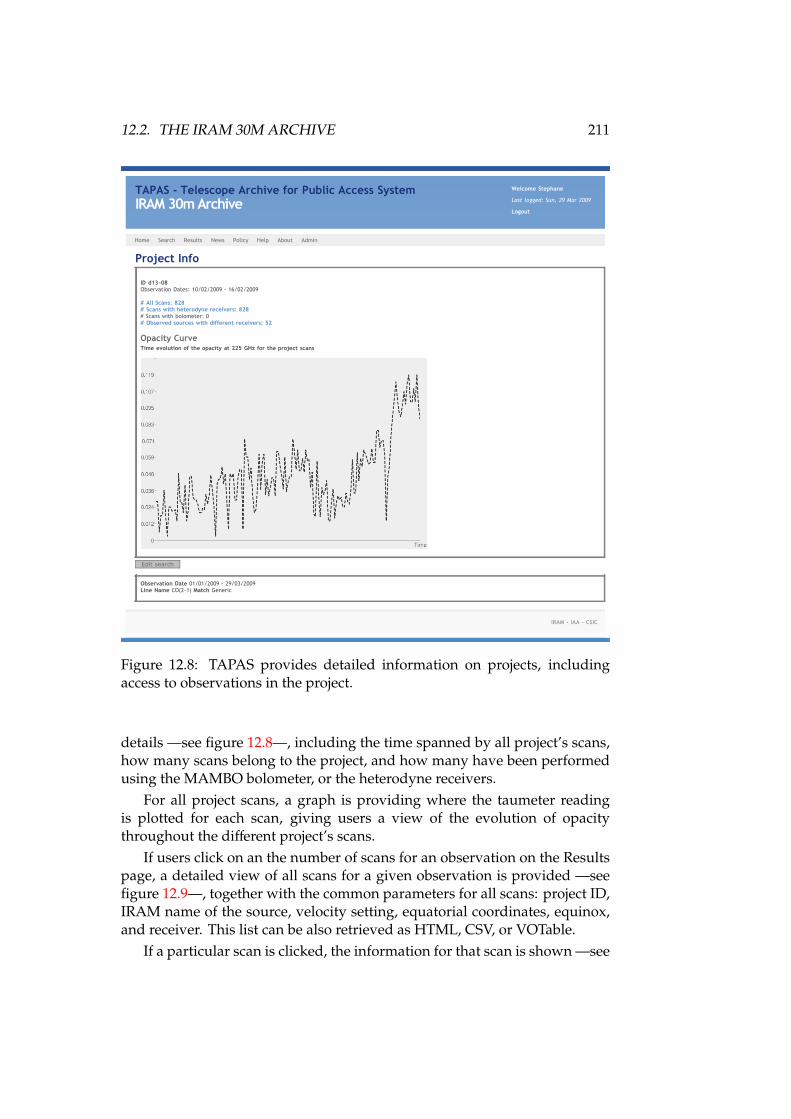
12.2. THE IRAM 30M ARCHIVE 211
Project Info ID d13-08Observation Dates: 10/02/2009 - 16/02/2009
# All Scans: 828# Scans with heterodyne receivers: 828# Scans with bolometer: 0# Observed sources with different receivers: 52
Opacity CurveTime evolution of the opacity at 225 GHz for the project scans
Edit search
Observation Date 01/01/2009 - 29/03/2009Line Name CO(2-1) Match Generic
IRAM - IAA - CSIC
Home Search Results News Policy Help About Admin
TAPAS - Telescope Archive for Public Access SystemIRAM 30m Archive
Welcome Stephane
Last logged: Sun, 29 Mar 2009
Logout
Figure 12.8: TAPAS provides detailed information on projects, includingaccess to observations in the project.
details —see figure 12.8—, including the time spanned by all project’s scans,how many scans belong to the project, and how many have been performedusing the MAMBO bolometer, or the heterodyne receivers.
For all project scans, a graph is providing where the taumeter readingis plotted for each scan, giving users a view of the evolution of opacitythroughout the different project’s scans.
If users click on an the number of scans for an observation on the Resultspage, a detailed view of all scans for a given observation is provided —seefigure 12.9—, together with the common parameters for all scans: project ID,IRAM name of the source, velocity setting, equatorial coordinates, equinox,and receiver. This list can be also retrieved as HTML, CSV, or VOTable.
If a particular scan is clicked, the information for that scan is shown —see
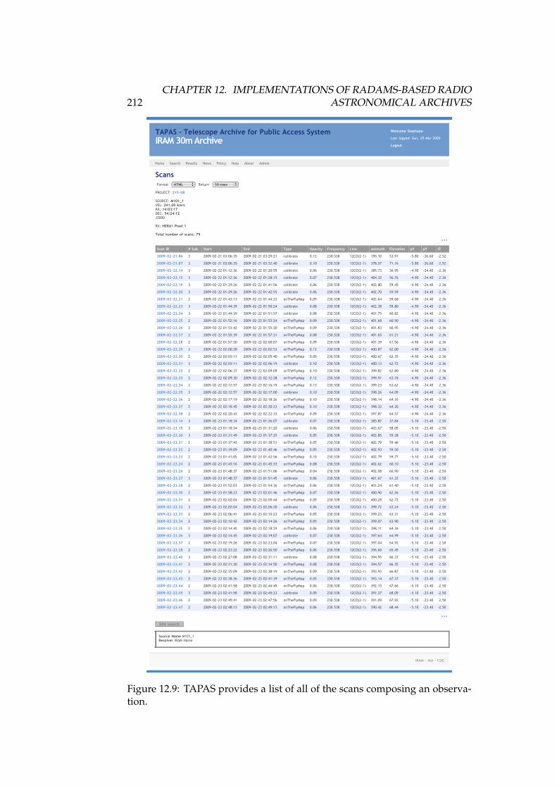
212CHAPTER 12. IMPLEMENTATIONS OF RADAMS-BASED RADIO
ASTRONOMICAL ARCHIVES
ScansFormat HTML Return 50 rows
PROJECT: 215-08
SOURCE: M101_1VEL: 241.00 km/sRA: 14:03:17DEC: 54:24:12J2000
RX: HERA1 Pixel 1
Total number of scans: 79
>>>
Scan ID # Sub. Start End Type Opacity Frequency Line Azimuth Elevation pX pY fZ
2009-02-21.86 3 2009-02-21 03:06:35 2009-02-21 03:29:21 calibrate 0.12 230.538 12CO(2-1) 195.10 53.91 -5.80 -26.60 -2.52
2009-02-21.87 3 2009-02-21 03:06:35 2009-02-21 03:32:40 calibrate 0.10 230.538 12CO(2-1) 378.57 71.16 -5.80 -26.60 -2.52
2009-02-22.14 3 2009-02-22 01:12:36 2009-02-22 01:20:55 calibrate 0.06 230.538 12CO(2-1) 385.73 36.95 -4.90 -24.40 -2.36
2009-02-22.15 3 2009-02-22 01:12:36 2009-02-22 01:28:15 calibrate 0.07 230.538 12CO(2-1) 404.32 56.76 -4.90 -24.40 -2.36
2009-02-22.19 3 2009-02-22 01:29:26 2009-02-22 01:41:56 calibrate 0.06 230.538 12CO(2-1) 402.80 59.45 -4.90 -24.40 -2.36
2009-02-22.20 3 2009-02-22 01:29:26 2009-02-22 01:42:55 calibrate 0.06 230.538 12CO(2-1) 402.70 59.59 -4.90 -24.40 -2.36
2009-02-22.21 2 2009-02-22 01:43:13 2009-02-22 01:44:22 onTheFlyMap 0.09 230.538 12CO(2-1) 402.64 59.68 -4.90 -24.40 -2.36
2009-02-22.23 3 2009-02-22 01:44:39 2009-02-22 01:50:24 calibrate 0.08 230.538 12CO(2-1) 402.38 59.80 -4.90 -24.40 -2.36
2009-02-22.24 3 2009-02-22 01:44:39 2009-02-22 01:51:57 calibrate 0.08 230.538 12CO(2-1) 401.75 60.82 -4.90 -24.40 -2.36
2009-02-22.25 2 2009-02-22 01:52:16 2009-02-22 01:53:24 onTheFlyMap 0.09 230.538 12CO(2-1) 401.68 60.90 -4.90 -24.40 -2.36
2009-02-22.26 2 2009-02-22 01:53:42 2009-02-22 01:55:20 onTheFlyMap 0.09 230.538 12CO(2-1) 401.83 60.95 -4.90 -24.40 -2.36
2009-02-22.27 2 2009-02-22 01:55:39 2009-02-22 01:57:31 onTheFlyMap 0.08 230.538 12CO(2-1) 401.65 61.21 -4.90 -24.40 -2.36
2009-02-22.28 2 2009-02-22 01:57:50 2009-02-22 02:00:07 onTheFlyMap 0.09 230.538 12CO(2-1) 401.39 61.56 -4.90 -24.40 -2.36
2009-02-22.29 2 2009-02-22 02:00:28 2009-02-22 02:02:53 onTheFlyMap 0.12 230.538 12CO(2-1) 400.87 62.00 -4.90 -24.40 -2.36
2009-02-22.30 2 2009-02-22 02:03:11 2009-02-22 02:05:40 onTheFlyMap 0.09 230.538 12CO(2-1) 400.67 62.35 -4.90 -24.40 -2.36
2009-02-22.31 3 2009-02-22 02:03:11 2009-02-22 02:06:19 calibrate 0.10 230.538 12CO(2-1) 400.13 62.72 -4.90 -24.40 -2.36
2009-02-22.32 2 2009-02-22 02:06:37 2009-02-22 02:09:09 onTheFlyMap 0.10 230.538 12CO(2-1) 399.82 62.80 -4.90 -24.40 -2.36
2009-02-22.33 2 2009-02-22 02:09:30 2009-02-22 02:12:38 onTheFlyMap 0.12 230.538 12CO(2-1) 399.91 63.18 -4.90 -24.40 -2.36
2009-02-22.34 2 2009-02-22 02:12:57 2009-02-22 02:16:19 onTheFlyMap 0.13 230.538 12CO(2-1) 399.23 63.62 -4.90 -24.40 -2.36
2009-02-22.35 3 2009-02-22 02:12:57 2009-02-22 02:17:00 calibrate 0.10 230.538 12CO(2-1) 398.26 64.09 -4.90 -24.40 -2.36
2009-02-22.36 2 2009-02-22 02:17:19 2009-02-22 02:18:26 onTheFlyMap 0.10 230.538 12CO(2-1) 398.14 64.16 -4.90 -24.40 -2.36
2009-02-22.37 2 2009-02-22 02:18:45 2009-02-22 02:20:23 onTheFlyMap 0.10 230.538 12CO(2-1) 398.32 64.20 -4.90 -24.40 -2.36
2009-02-22.38 2 2009-02-22 02:20:43 2009-02-22 02:22:33 onTheFlyMap 0.09 230.538 12CO(2-1) 397.87 64.57 -4.90 -24.40 -2.36
2009-02-23.14 3 2009-02-23 01:18:34 2009-02-23 01:26:07 calibrate 0.07 230.538 12CO(2-1) 385.87 37.84 -5.10 -23.40 -2.50
2009-02-23.15 3 2009-02-23 01:18:34 2009-02-23 01:31:20 calibrate 0.06 230.538 12CO(2-1) 403.67 58.05 -5.10 -23.40 -2.50
2009-02-23.20 3 2009-02-23 01:31:49 2009-02-23 01:37:25 calibrate 0.05 230.538 12CO(2-1) 402.85 59.38 -5.10 -23.40 -2.50
2009-02-23.21 2 2009-02-23 01:37:43 2009-02-23 01:38:51 onTheFlyMap 0.05 230.538 12CO(2-1) 402.79 59.46 -5.10 -23.40 -2.50
2009-02-23.22 2 2009-02-23 01:39:09 2009-02-23 01:40:46 onTheFlyMap 0.05 230.538 12CO(2-1) 402.93 59.50 -5.10 -23.40 -2.50
2009-02-23.23 2 2009-02-23 01:41:05 2009-02-23 01:42:56 onTheFlyMap 0.10 230.538 12CO(2-1) 402.79 59.77 -5.10 -23.40 -2.50
2009-02-23.24 2 2009-02-23 01:43:16 2009-02-23 01:45:33 onTheFlyMap 0.08 230.538 12CO(2-1) 402.62 60.10 -5.10 -23.40 -2.50
2009-02-23.26 2 2009-02-23 01:48:37 2009-02-23 01:51:06 onTheFlyMap 0.04 230.538 12CO(2-1) 402.08 60.90 -5.10 -23.40 -2.50
2009-02-23.27 3 2009-02-23 01:48:37 2009-02-23 01:51:45 calibrate 0.06 230.538 12CO(2-1) 401.67 61.32 -5.10 -23.40 -2.50
2009-02-23.28 2 2009-02-23 01:52:03 2009-02-23 01:54:36 onTheFlyMap 0.06 230.538 12CO(2-1) 401.24 61.40 -5.10 -23.40 -2.50
2009-02-23.30 2 2009-02-23 01:58:23 2009-02-23 02:01:46 onTheFlyMap 0.07 230.538 12CO(2-1) 400.90 62.26 -5.10 -23.40 -2.50
2009-02-23.31 2 2009-02-23 02:02:04 2009-02-23 02:05:44 onTheFlyMap 0.05 230.538 12CO(2-1) 400.28 62.72 -5.10 -23.40 -2.50
2009-02-23.32 3 2009-02-23 02:02:04 2009-02-23 02:06:20 calibrate 0.06 230.538 12CO(2-1) 399.72 63.24 -5.10 -23.40 -2.50
2009-02-23.33 2 2009-02-23 02:06:41 2009-02-23 02:10:23 onTheFlyMap 0.05 230.538 12CO(2-1) 399.23 63.31 -5.10 -23.40 -2.50
2009-02-23.34 2 2009-02-23 02:10:42 2009-02-23 02:14:26 onTheFlyMap 0.05 230.538 12CO(2-1) 399.07 63.90 -5.10 -23.40 -2.50
2009-02-23.35 2 2009-02-23 02:14:45 2009-02-23 02:18:29 onTheFlyMap 0.06 230.538 12CO(2-1) 398.11 64.34 -5.10 -23.40 -2.50
2009-02-23.36 3 2009-02-23 02:14:45 2009-02-23 02:19:07 calibrate 0.07 230.538 12CO(2-1) 397.64 64.99 -5.10 -23.40 -2.50
2009-02-23.37 2 2009-02-23 02:19:26 2009-02-23 02:23:04 onTheFlyMap 0.07 230.538 12CO(2-1) 397.04 64.92 -5.10 -23.40 -2.50
2009-02-23.38 2 2009-02-23 02:23:22 2009-02-23 02:26:50 onTheFlyMap 0.06 230.538 12CO(2-1) 396.60 65.45 -5.10 -23.40 -2.50
2009-02-23.40 3 2009-02-23 02:27:08 2009-02-23 02:31:11 calibrate 0.08 230.538 12CO(2-1) 394.95 66.37 -5.10 -23.40 -2.50
2009-02-23.41 2 2009-02-23 02:31:30 2009-02-23 02:34:50 onTheFlyMap 0.08 230.538 12CO(2-1) 394.57 66.35 -5.10 -23.40 -2.50
2009-02-23.42 2 2009-02-23 02:35:09 2009-02-23 02:38:19 onTheFlyMap 0.09 230.538 12CO(2-1) 393.93 66.87 -5.10 -23.40 -2.50
2009-02-23.43 2 2009-02-23 02:38:36 2009-02-23 02:41:39 onTheFlyMap 0.05 230.538 12CO(2-1) 393.14 67.37 -5.10 -23.40 -2.50
2009-02-23.44 2 2009-02-23 02:41:58 2009-02-23 02:44:45 onTheFlyMap 0.06 230.538 12CO(2-1) 392.15 67.66 -5.10 -23.40 -2.50
2009-02-23.45 3 2009-02-23 02:41:58 2009-02-23 02:45:23 calibrate 0.09 230.538 12CO(2-1) 391.37 68.09 -5.10 -23.40 -2.50
2009-02-23.46 2 2009-02-23 02:45:41 2009-02-23 02:47:56 onTheFlyMap 0.09 230.538 12CO(2-1) 391.09 67.92 -5.10 -23.40 -2.50
2009-02-23.47 2 2009-02-23 02:48:13 2009-02-23 02:49:13 onTheFlyMap 0.06 230.538 12CO(2-1) 390.42 68.44 -5.10 -23.40 -2.50
>>>
Edit search
Source Name M101_1Resolver IRAM Name
IRAM - IAA - CSIC
Home Search Results News Policy Help About Admin
TAPAS - Telescope Archive for Public Access SystemIRAM 30m Archive
Welcome Stephane
Last logged: Sun, 29 Mar 2009
Logout
Figure 12.9: TAPAS provides a list of all of the scans composing an observa-tion.
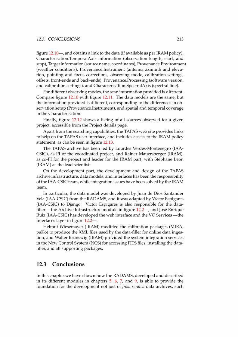
12.3. CONCLUSIONS 213
figure 12.10—, and obtains a link to the data (if available as per IRAM policy),Characterisation.TemporalAxis information (observation length, start, andstop), Target information (source name, coordinates), Provenance.Environment(weather conditions), Provenance.Instrument (antenna azimuth and eleva-tion, pointing and focus corrections, observing mode, calibration settings,offsets, front-ends and back-ends), Provenance.Processing (software version,and calibration settings), and Characterisation.SpectralAxis (spectral line).
For different observing modes, the scan information provided is different.Compare figure 12.10 with figure 12.11. The data models are the same, butthe information provided is different, corresponding to the differences in ob-servation setup (Provenance.Instrument), and spatial and temporal coveragein the Characterisation.
Finally, figure 12.12 shows a listing of all sources observed for a givenproject, accessible from the Project details page.
Apart from the searching capabilities, the TAPAS web site provides linksto help on the TAPAS user interface, and includes access to the IRAM policystatement, as can be seen in figure 12.13.
The TAPAS archive has been led by Lourdes Verdes-Montenegro (IAA-CSIC), as PI of the coordinated project, and Rainer Mauersberger (IRAM),as co-PI for the project and leader for the IRAM part, with Stéphane Leon(IRAM) as the lead scientist.
On the development part, the development and design of the TAPASarchive infrastructure, data models, and interfaces has been the responsibilityof the IAA-CSIC team, while integration issues have been solved by the IRAMteam.
In particular, the data model was developed by Juan de Dios SantanderVela (IAA-CSIC) from the RADAMS, and it was adapted by Víctor Espigares(IAA-CSIC) to Django. Victor Espigares is also responsible for the data-filler —the Archive Infrastructure module in figure 12.2—, and José EnriqueRuiz (IAA-CSIC) has developed the web interface and the VO Services —theInterfaces layer in figure 12.2—.
Helmut Wiesemayer (IRAM) modified the calibration packages (MIRA,paKo) to produce the XML files used by the data-filler for online data inges-tion, and Walter Brunswig (IRAM) provided the system integration servicesin the New Control System (NCS) for accessing FITS files, installing the data-filler, and all supporting packages.
12.3 Conclusions
In this chapter we have shown how the RADAMS, developed and describedin its different modules in chapters 5, 6, 7, and 9, is able to provide thefoundation for the development not just of from scratch data archives, such
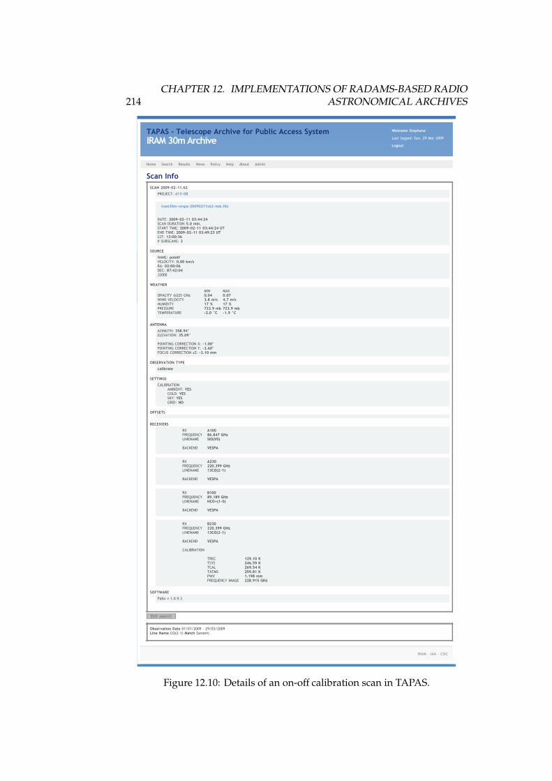
214CHAPTER 12. IMPLEMENTATIONS OF RADAMS-BASED RADIO
ASTRONOMICAL ARCHIVES
Scan InfoSCAN 2009-02-11.62
PROJECT: d13-08
iram30m-vespa-20090211s62-imb.fits
DATE: 2009-02-11 03:44:24SCAN DURATION 5.0 min.START TIME: 2009-02-11 03:44:24 UTEND TIME: 2009-02-11 03:49:23 UTLST: 13:00:36# SUBSCANS: 3
SOURCE
NAME: polotfVELOCITY: 0.00 km/sRA: 02:00:06 DEC: 87:42:04J2000
WEATHER
MIN MAXOPACITY @225 GHz 0.04 0.07WIND VELOCITY 3.8 m/s 4.7 m/sHUMIDITY 17 % 17 %PRESSURE 723.9 mb 723.9 mbTEMPERATURE -2.0 °C -1.9 °C
ANTENNA
AZIMUTH: 358.94°ELEVATION: 35.09°
POINTING CORRECTION X: -1.00"POINTING CORRECTION Y: -3.60"FOCUS CORRECTION zZ: -3.10 mm
OBSERVATION TYPE
calibrate
SETTINGS
CALIBRATION AMBIENT: YES COLD: YES SKY: YES GRID: NO
OFFSETS
RECEIVERS
RX A100FREQUENCY 86.847 GHzLINENAME SIO(V0)
BACKEND VESPA
RX A230FREQUENCY 220.399 GHzLINENAME 13CO(2-1)
BACKEND VESPA
RX B100FREQUENCY 89.189 GHzLINENAME HCO+(1-0)
BACKEND VESPA
RX B230FREQUENCY 220.399 GHzLINENAME 13CO(2-1)
BACKEND VESPA
CALIBRATION
TREC 129.10 KTSYS 246.59 KTCAL 269.54 KTATMS 259.81 KPWV 1.198 mmFREQUENCY IMAGE 228.915 GHz
SOFTWARE
PaKo v 1.0.9.3
Edit search
Observation Date 01/01/2009 - 29/03/2009Line Name CO(2-1) Match Generic
IRAM - IAA - CSIC
Home Search Results News Policy Help About Admin
TAPAS - Telescope Archive for Public Access SystemIRAM 30m Archive
Welcome Stephane
Last logged: Sun, 29 Mar 2009
Logout
Figure 12.10: Details of an on-off calibration scan in TAPAS.
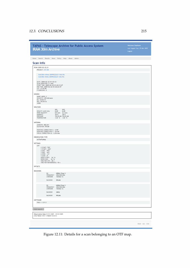
12.3. CONCLUSIONS 215
Scan InfoSCAN 2009-02-22.21
PROJECT: 215-08
iram30m-wilma-20090222s21-imb.fitsiram30m-4mhz-20090222s21-imb.fits
DATE: 2009-02-22 01:43:13SCAN DURATION 1.1 min.START TIME: 2009-02-22 01:43:13 UTEND TIME: 2009-02-22 01:44:22 UTLST: 11:37:49# SUBSCANS: 2
SOURCE
NAME: M101_1VELOCITY: 241.00 km/sRA: 14:03:17 DEC: 54:24:12J2000
WEATHER
MIN MAXOPACITY @225 GHz 0.09 0.09WIND VELOCITY 0.9 m/s 2.3 m/sHUMIDITY 18 % 18 %PRESSURE 723.8 mb 723.8 mbTEMPERATURE -3.8 °C -3.8 °C
ANTENNA
AZIMUTH: 402.64°ELEVATION: 59.68°
POINTING CORRECTION X: -4.90"POINTING CORRECTION Y: -24.40"FOCUS CORRECTION zZ: -2.36 mm
OBSERVATION TYPE
onTheFlyMap
SETTINGS
OTF X START: 792" Y START: -323" X END: 792" Y END: 161" X STEP: -11" Y STEP: 0" SPEED START: 16 "/s SPEED END: 16 "/s TIME PER OTF: 30 s TIME PER REFERERENCE: 10 s
OFFSETS
RECEIVERS
RX HERA1 Pixel 1FREQUENCY 230.538 GHzLINENAME 12CO(2-1)
BACKEND WILMA
RX HERA2 Pixel 1FREQUENCY 230.538 GHzLINENAME 12CO(2-1)
BACKEND 4MHz
BACKEND WILMA
SOFTWARE
PaKo v 1.0.9.3
Edit search
Observation Date 01/01/2009 - 29/03/2009Line Name CO(2-1) Match Generic
IRAM - IAA - CSIC
Home Search Results News Policy Help About Admin
TAPAS - Telescope Archive for Public Access SystemIRAM 30m Archive
Welcome Stephane
Last logged: Sun, 29 Mar 2009
Logout
Figure 12.11: Details for a scan belonging to an OTF map.
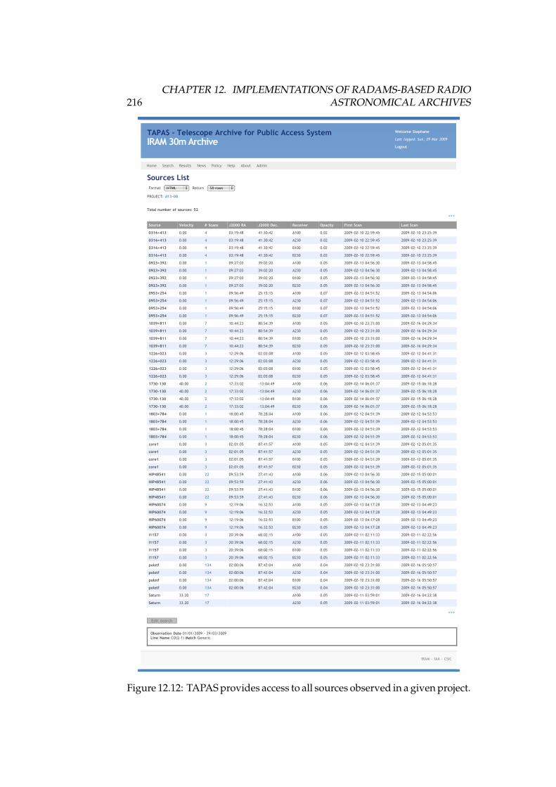
216CHAPTER 12. IMPLEMENTATIONS OF RADAMS-BASED RADIO
ASTRONOMICAL ARCHIVES
Sources ListFormat HTML Return 50 rows
PROJECT: d13-08
Total number of sources: 52
>>>
Source Velocity # Scans J2000 RA J2000 Dec. Receiver Opacity First Scan Last Scan
0316+413 0.00 4 03:19:48 41:30:42 A100 0.02 2009-02-10 22:59:45 2009-02-10 23:25:39
0316+413 0.00 4 03:19:48 41:30:42 A230 0.02 2009-02-10 22:59:45 2009-02-10 23:25:39
0316+413 0.00 4 03:19:48 41:30:42 B100 0.02 2009-02-10 22:59:45 2009-02-10 23:25:39
0316+413 0.00 4 03:19:48 41:30:42 B230 0.02 2009-02-10 22:59:45 2009-02-10 23:25:39
0923+392 0.00 1 09:27:03 39:02:20 A100 0.05 2009-02-13 04:56:30 2009-02-13 04:58:45
0923+392 0.00 1 09:27:03 39:02:20 A230 0.05 2009-02-13 04:56:30 2009-02-13 04:58:45
0923+392 0.00 1 09:27:03 39:02:20 B100 0.05 2009-02-13 04:56:30 2009-02-13 04:58:45
0923+392 0.00 1 09:27:03 39:02:20 B230 0.05 2009-02-13 04:56:30 2009-02-13 04:58:45
0953+254 0.00 1 09:56:49 25:15:15 A100 0.07 2009-02-13 04:51:52 2009-02-13 04:54:06
0953+254 0.00 1 09:56:49 25:15:15 A230 0.07 2009-02-13 04:51:52 2009-02-13 04:54:06
0953+254 0.00 1 09:56:49 25:15:15 B100 0.07 2009-02-13 04:51:52 2009-02-13 04:54:06
0953+254 0.00 1 09:56:49 25:15:15 B230 0.07 2009-02-13 04:51:52 2009-02-13 04:54:06
1039+811 0.00 7 10:44:23 80:54:39 A100 0.05 2009-02-10 23:31:00 2009-02-16 04:29:34
1039+811 0.00 7 10:44:23 80:54:39 A230 0.05 2009-02-10 23:31:00 2009-02-16 04:29:34
1039+811 0.00 7 10:44:23 80:54:39 B100 0.05 2009-02-10 23:31:00 2009-02-16 04:29:34
1039+811 0.00 7 10:44:23 80:54:39 B230 0.05 2009-02-10 23:31:00 2009-02-16 04:29:34
1226+023 0.00 3 12:29:06 02:03:08 A100 0.05 2009-02-12 03:58:45 2009-02-12 04:41:31
1226+023 0.00 3 12:29:06 02:03:08 A230 0.05 2009-02-12 03:58:45 2009-02-12 04:41:31
1226+023 0.00 3 12:29:06 02:03:08 B100 0.05 2009-02-12 03:58:45 2009-02-12 04:41:31
1226+023 0.00 3 12:29:06 02:03:08 B230 0.05 2009-02-12 03:58:45 2009-02-12 04:41:31
1730-130 40.00 2 17:33:02 -13:04:49 A100 0.06 2009-02-14 06:01:37 2009-02-15 06:18:28
1730-130 40.00 2 17:33:02 -13:04:49 A230 0.06 2009-02-14 06:01:37 2009-02-15 06:18:28
1730-130 40.00 2 17:33:02 -13:04:49 B100 0.06 2009-02-14 06:01:37 2009-02-15 06:18:28
1730-130 40.00 2 17:33:02 -13:04:49 B230 0.06 2009-02-14 06:01:37 2009-02-15 06:18:28
1803+784 0.00 1 18:00:45 78:28:04 A100 0.06 2009-02-12 04:51:39 2009-02-12 04:53:53
1803+784 0.00 1 18:00:45 78:28:04 A230 0.06 2009-02-12 04:51:39 2009-02-12 04:53:53
1803+784 0.00 1 18:00:45 78:28:04 B100 0.06 2009-02-12 04:51:39 2009-02-12 04:53:53
1803+784 0.00 1 18:00:45 78:28:04 B230 0.06 2009-02-12 04:51:39 2009-02-12 04:53:53
core1 0.00 3 02:01:05 87:41:57 A100 0.05 2009-02-12 04:51:39 2009-02-12 05:01:35
core1 0.00 3 02:01:05 87:41:57 A230 0.05 2009-02-12 04:51:39 2009-02-12 05:01:35
core1 0.00 3 02:01:05 87:41:57 B100 0.05 2009-02-12 04:51:39 2009-02-12 05:01:35
core1 0.00 3 02:01:05 87:41:57 B230 0.05 2009-02-12 04:51:39 2009-02-12 05:01:35
HIP48541 0.00 22 09:53:59 27:41:43 A100 0.06 2009-02-13 04:56:30 2009-02-15 05:00:01
HIP48541 0.00 22 09:53:59 27:41:43 A230 0.06 2009-02-13 04:56:30 2009-02-15 05:00:01
HIP48541 0.00 22 09:53:59 27:41:43 B100 0.06 2009-02-13 04:56:30 2009-02-15 05:00:01
HIP48541 0.00 22 09:53:59 27:41:43 B230 0.06 2009-02-13 04:56:30 2009-02-15 05:00:01
HIP60074 0.00 9 12:19:06 16:32:53 A100 0.05 2009-02-13 04:17:28 2009-02-13 04:49:23
HIP60074 0.00 9 12:19:06 16:32:53 A230 0.05 2009-02-13 04:17:28 2009-02-13 04:49:23
HIP60074 0.00 9 12:19:06 16:32:53 B100 0.05 2009-02-13 04:17:28 2009-02-13 04:49:23
HIP60074 0.00 9 12:19:06 16:32:53 B230 0.05 2009-02-13 04:17:28 2009-02-13 04:49:23
l1157 0.00 3 20:39:06 68:02:15 A100 0.05 2009-02-11 02:11:33 2009-02-11 02:22:56
l1157 0.00 3 20:39:06 68:02:15 A230 0.05 2009-02-11 02:11:33 2009-02-11 02:22:56
l1157 0.00 3 20:39:06 68:02:15 B100 0.05 2009-02-11 02:11:33 2009-02-11 02:22:56
l1157 0.00 3 20:39:06 68:02:15 B230 0.05 2009-02-11 02:11:33 2009-02-11 02:22:56
polotf 0.00 134 02:00:06 87:42:04 A100 0.04 2009-02-10 23:31:00 2009-02-16 05:50:57
polotf 0.00 134 02:00:06 87:42:04 A230 0.04 2009-02-10 23:31:00 2009-02-16 05:50:57
polotf 0.00 134 02:00:06 87:42:04 B100 0.04 2009-02-10 23:31:00 2009-02-16 05:50:57
polotf 0.00 134 02:00:06 87:42:04 B230 0.04 2009-02-10 23:31:00 2009-02-16 05:50:57
Saturn 33.20 17 A100 0.05 2009-02-11 03:59:01 2009-02-16 04:22:38
Saturn 33.20 17 A230 0.05 2009-02-11 03:59:01 2009-02-16 04:22:38
>>>
Edit search
Observation Date 01/01/2009 - 29/03/2009Line Name CO(2-1) Match Generic
IRAM - IAA - CSIC
Home Search Results News Policy Help About Admin
TAPAS - Telescope Archive for Public Access SystemIRAM 30m Archive
Welcome Stephane
Last logged: Sun, 29 Mar 2009
Logout
Figure 12.12: TAPAS provides access to all sources observed in a given project.

12.3. CONCLUSIONS 217
IRAM - IAA - CSIC
Home Search Results News Policy Help About Admin
PolicyTAPAS contains header information of all astronomical data taken after 01/01/2009. TAPAS does not contain any astronomical heterodyne or bolometer data. However, TAPASprovides the possibility to link the header data of individual scans to FITS files containing the uncalibrated astronomical data. TAPAS provides a Virtual Observatory facility forquery and retrieval of header data.
Access rights to any astronomical data in TAPAS depend on the project. The PI and IRAM decide when to make astronomical data public. For all projects, after a proprietaryperiod of one year, a subset of header data will be made accessible via web interfaces and search tools. IRAM staff have immediate and unrestricted access to all header data.For large programs, access to all data will be granted after a 18 months proprietary period. The proprietary period starts when the last observations of a given project arefinished.
TAPAS - Telescope Archive for Public Access SystemIRAM 30m Archive
Welcome Stephane
Last logged: Sun, 29 Mar 2009
Logout
Figure 12.13: TAPAS policy, as specified by the IRAM.
as that for the DSS-63 antenna, but also for archives being built on top of anexisting archival infrastructure, such as that of the IRAM 30m antenna.
The many different observing modes, frontends, backends, mappingsbetween frontend and backends, and the need to support both raw and pro-cessed data, have enriched the RADAMS with respect to its initial incarnation,to the point of providing the desired basis.
In the case of the IRAM 30m archive, the IRAM data access policy (noactual data available through the archive interface at least for 18 monthssince the end of an observing project, and access to header —pointing andobserving configuration— information for observations after 12 months) havecontributed to validate the Policy data model, and the Instrument, SoftwareProcessing and Calibration Provenance.

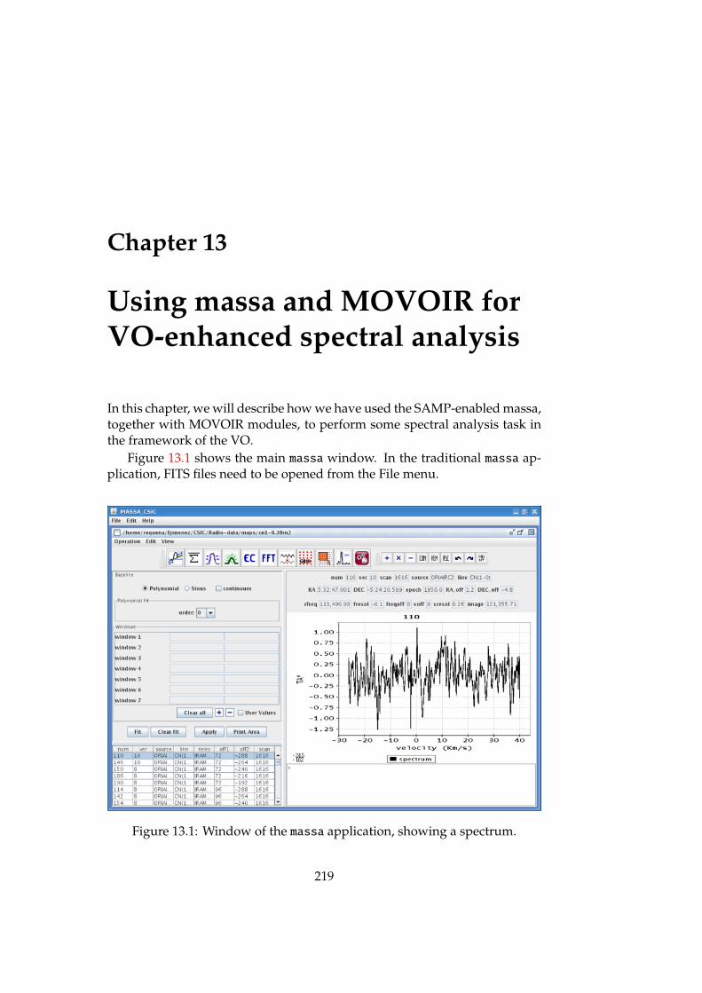
Chapter 13
Using massa and MOVOIR forVO-enhanced spectral analysis
In this chapter, we will describe how we have used the SAMP-enabled massa,together with MOVOIR modules, to perform some spectral analysis task inthe framework of the VO.
Figure 13.1 shows the main massa window. In the traditional massa ap-plication, FITS files need to be opened from the File menu.
Figure 13.1: Window of the massa application, showing a spectrum.
219

220CHAPTER 13. USING MASSA AND MOVOIR FOR VO-ENHANCED
SPECTRAL ANALYSIS
Figure 13.2: SAMP Hub, showing TOPCAT and VODownloader. By havingVODownloader selected, we can see all the messages it is subscribed to.
In figure 13.2 the main window of the JSAMP Hub shows the differentregistered modules. By selecting one of the applications in the list, one caninspect the different messages each application is subscribed to. We can seein the picture that VODownloader is subscribed to samp.* administrativemethods, and to table.load.votable, image.load.fits, and the MOVOIRspecific url.load.file.
Figure 13.3, on the other hand, shows the VODownloader window, afterhaving received a table.load.votable message from TOPCAT. If users clickon a download, they can discover the file in the system’s file browser, orre-send it to another SAMP-enabled application.
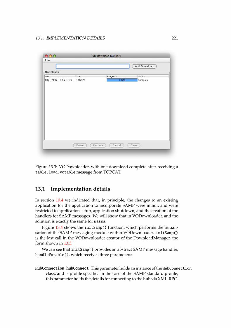
13.1. IMPLEMENTATION DETAILS 221
Figure 13.3: VODownloader, with one download complete after receiving atable.load.votable message from TOPCAT.
13.1 Implementation details
In section 10.4 we indicated that, in principle, the changes to an existingapplication for the application to incorporate SAMP were minor, and wererestricted to application setup, application shutdown, and the creation of thehandlers for SAMP messages. We will show that in VODownloader, and thesolution is exactly the same for massa.
Figure 13.4 shows the initSamp() function, which performs the initiali-sation of the SAMP messaging module within VODownloader. initSamp()is the last call in the VODownloader creator of the DownloadManager, theform shown in 13.3.
We can see that initSamp() provides an abstract SAMP message handler,handleVotable(), which receives three parameters:
HubConnection hubConnect This parameter holds an instance of theHubConnectionclass, and is profile specific. In the case of the SAMP standard profile,this parameter holds the details for connecting to the hub via XML-RPC.
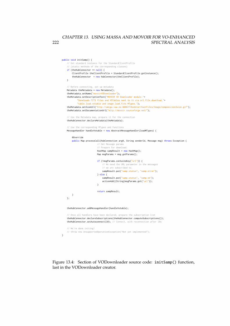
222CHAPTER 13. USING MASSA AND MOVOIR FOR VO-ENHANCED
SPECTRAL ANALYSIS
public void initSamp() // Get standard instance for the StandardClientProfile // (static methods of the corresponding classes) if (theHubConnector == null) ClientProfile theClientProfile = StandardClientProfile.getInstance(); theHubConnector = new HubConnector(theClientProfile); // Before connecting, set up metadata Metadata theMetadata = new Metadata(); theMetadata.setName("movoirVODownloader"); theMetadata.setDescriptionText("MOVOIR VO Downloader module."+ "Donwloads FITS files and VOTables sent to it via url.file.download,"+ "table.load.votable and image.load.fits MTypes."); theMetadata.setIconUrl("http://amiga.iaa.es:8080/FCKeditor/UserFiles/Image/composicion3size.gif"); theMetadata.setDocumentationUrl("http://movoir.sourceforge.net/"); // Use the Metadata map, prepare it for the connection theHubConnector.declareMetadata(theMetadata); // Use the corresponding MTypes and functions MessageHandler handleVotable = new AbstractMessageHandler(loadMTypes) @Override public Map processCall(HubConnection arg0, String senderId, Message msg) throws Exception // Get Message params // Prepare for download: HashMap sampResult = new HashMap(); Map msgParams = msg.getParams(); if (!msgParams.containsKey("url")) // We need the URL parameter in the messages // we are subscribed to. sampResult.put("samp.status", "samp.error"); else sampResult.put("samp.status", "samp.ok"); actionAdd((String)msgParams.get("url")); return sampResult; ; theHubConnector.addMessageHandler(handleVotable); // Once all handlers have been declared, prepare the subscription list theHubConnector.declareSubscriptions(theHubConnector.computeSubscriptions()); theHubConnector.setAutoconnect(10); // Connect, with reconnection after 10s // We're done initing! // throw new UnsupportedOperationException("Not yet implemented");
Figure 13.4: Section of VODownloader source code: initSamp() function,last in the VODownloader creator.

13.2. CONCLUSIONS 223
String senderId This parameter provides a string with the unique identifierof the application that sent (or broadcasted) a message to our handler.We will use this in order to create messages back to the sender with theresult of our computations. In the case of VODownloader, the resultsis always a samp.ok answer, or a samp.error if the message does notprovide a url parameter within the samp.params map.
Message msg The msg parameter is the map described in section 11.1, andprovides all the actual message information: samp.mtype, for choosingthe function to be performed, and samp.params for the function to work.
In the case of VODownloader, the messages which are implemented aretable.load.votable, image.load.fits, and table.load.fits (passed as alist of MType strings in loadMTypes). All of those messages need to providea url parameter.
If url present, the actionAdd(String urlString) method is called inorder to queue the download of the corresponding data. We can see that theactionAdd method already existed in VODownloader, and our handler justdelegates the actual behaviour to an already existing function.
An additional shutdownSamp() method is called from the actionExit()method. Following the flow diagram shown in figure 10.4, we have justmodified:
VODownloader creator We have added an initSamp method to declare themessages we are prepared to handle, at the end of the creator of theDownloadManager class of the VODownload.
Event handling The event handling is modified by the sameinitSampmethod,by adding listeners to SAMP messages with the addMessageHandlermethod. The message handler uses existing controller methods to del-egate the actual implementation of the handler.
VODownloader shutdown In the case of the VODownloader, the origi-nal DownloadManager shutdown is handled by the the actionExitmethod, and the shutdown of the SAMP messaging in VODownloaderis implemented as the first function in that method. For other applica-tions, equivalent placements, if possible within a guaranteed executionthread, need to be chosen.
13.2 Conclusions
By developing a SAMP-based approach for the MOVOIR, we have beenable to VO-enable massa with minimal changes, and at the same time wehave provided a mechanism for enhancing not only massa, but any existingSAMP-enabled application.

224CHAPTER 13. USING MASSA AND MOVOIR FOR VO-ENHANCED
SPECTRAL ANALYSIS
The minimum degree of VO compatibility is provided by the VODown-loader, which enables other VO applications to send table.load.votable,or image.load.fits messages, and consolidate those files into a folder werelegacy applications can retrieve useful data.
We have also shown that the amount of code which has to be modifiedis minimum: code has to be added to initialise the SAMP messaging, andSAMP event handling, but that is achieved by just adding a single methodcall in the application initialisation, and the shutdown of SAMP messagingas the first method in the actionExit method handler.
Conclusions and future work
In this chapter we will summarise the conclusions of the different chapters:
• There was no all-encompassing, IVOA sanctioned, data model for astro-nomical observations, and in any case only work on visible wavelengthshad been performed.
• Once developed the missing parts of the IVOA ObsDM, plus the con-tribution of the CharDM, they can be used as blueprints for archivedevelopment, easing the development of VO-compatible services. Twoarchives, for the IRAM 30m and the DSS-63 antennas, have been devel-oped on that basis.
• The most specific part for radio astronomy is the Provenance datamodel, and more specifically the Provenance.Instrument sub-model.This part has been created in a modular way, so that other instrumentscan have their own description. In particular, extensibility for radiointerferometry has been particularly taken into account.
• We have provided complete metadata for the RADAMS, including FITSkeywords for some attributes, and Unified Content Descriptors (UCDs)for all attributes. In the IRAM 30m archive we have added units meta-data for all table attributes, and we are experimenting with semanticweb technologies, providing additional metadata on engineering data,such as pointing models, et cetera.
• We have shown that providing VO-compatibility using the SAMP mes-saging protocol, based on a publish/subscribe architecture, instead ofbuilding a full VO-client and user interface, allows the integration ofthe VO for legacy tools.
• We have shown, too, that the amount of source code which needs tobe changed within an application following the MVC (Model-View-Controller) paradigm is minimum, which simplifies both development,testing, and debugging. By delegating the actual management of mes-sages received to the controller methods, coupling is reduced.
225
226 CONCLUSIONS AND FUTURE WORK
• We have also shown different mechanisms for creating a plug-in archi-tecture with self-describing, dynamically updated, discoverable com-puting modules, able to work with all existing SAMP-enabled applica-tions without any modification to them.
Future work
In the future, I will work with the European Southern Observatory organisa-tion in archives and archive metadata within the IVOA, and will perform thefollowing tasks in collaboration with the team at the IAA:
• Submit the different RADAMS parts for approval to the IVOA DataModelling Working Group, for the final issuing of the Observation DataModel IVOA Recommendation.
• Generalise the RADAMS with support for interferometry, in collabora-tion with the ALMA Archive Team.
• Extend the use of semantic web technologies in the ESO as a substitutionmechanism for ESO Hierarchic Keywords.
• Propose the MOVOIR as a reference implementation for an IVOAsanctioned plug-in architecture, in order to allow better integration ofMOVOIR modules with plug-in aware applications, and create RADAMS-enabled MOVOIR modules.
Conclusiones y trabajo futuro
Pasamos a resumir las conclusiones de la tesis:
• No existía ningún modelo de datos sancionado por IVOA apropia-do para todas las observaciones astronómicas. Además, los modelosexistentes no soportaban las especificidades de las observaciones radioastronómicas.
• Se han desarrollado dos archivos, para las antenas IRAM 30m y DSS-63,utilizando como base el RADAMS. Se ha demostrado la viabilidad delmodelo de datos de Observaciones de IVOA, ampliado en las clases su-geridas y no implementadas, y suplementado con el modelo de datos deCaracterización de datos astronómicos como base de archivos radioas-tronómicos, facilitando su completa compatibilidad con el ObservatorioVirtual.
• La parte del modelo de datos más específica para radio astronomía esel modelo de datos Provenance (Procedencia), y más específicamenteel sub-model Provenance.Instrument. Al dividir modularmente Prove-nance, y que Provenance.Instrument sea a su vez modular, se permitela sustitución de esta parte del modelo por la descripción de cualquierotro instrumento. En particular, se ha tenido especialmente en cuenta laextensibilidad a interferómetros radio.
• Hemos proporcionado metadatos completos para el RADAMS, inclu-yendo palabras clave FITS para algunos atributos, y Unified ContentDescriptors (UCDs, Descriptores Universales de Contenidos) para to-dos los atributos. En el caso del archivo de IRAM 30m hemos añadidotablas de metadatos para unidades de todos los atributos de las tablas,y estamos experimentando con tecnologías de web semántica, para po-der proporcionar una mejor descripción de los datos correspondientesa seguimiento de valores de ingeniería.
• Hemos mostrado que si se proporciona compatibilidad con VO median-te el protocolo SAMP de mensajería, que está basado en una arquitecturapublicar/subscribir, en vez de crear dentro de la aplicación un cliente VO
227
228 CONCLUSIONES Y TRABAJO FUTURO
completo, con su correspondiente GUI, se puede proporcionar completafuncionalidad VO a aplicaciones pre-VO.
• Hemos demostrado también que la cantidad de código que hay quecambiar en una aplicación que sigue una arquitectura MVC (Model-View-Controller) es mínima, lo que permite simplificar tanto la imple-mentación, como la depuración: al delegar la gestión de la apertura, ola descarga, de los mensajes recibidos a los métodos del controlador, ladepuración se hace más sencilla.
• Hemos mostrado también diferentes mecanismos para crear una arqui-tectura de módulos de cómputo (plug-ins) auto-describibles, dinámi-camente actualizables, y que proporcionan funcionalidad a todas lasaplicaciones capaces de usar mensajería SAMP.
Trabajo futuro
En el futuro, trabajaré con la ESO (European Southern Observatory, Obser-vatory Europeo Austral) en la organización de sus archivos y sus metadatoscorrespondientes en el marco del IVOA, y realizaré las siguientes tareas encolaboración con el grupo del IAA:
• Someter las diferentes partes del RADAMS para su aprobación dentrodel IVOA Data Modelling Working Group, para la creación final deuna IVOA Recommendation correspondiente al Modelo de Datos deObservación.
• Generalizar el RADAMS para que soporte datos interferométricos, encolaboración con el ALMA Archive Team de la ESO.
• Extender el uso de tecnologías de web semántica en substitución delmecanismo ESO Hierarchic Keywords.
• Presentar en MOVOIR en los IVOA InterOp, y el ADASS (AstronomicalData Analysis Software and Systems), y obtener sugerencias de losusuarios para crear más módulos para el MOVOIR.
• Proponer MOVOIR como implementación de referencia para una arqui-tectura de plug-in sancionada por IVOA. Si se sanciona una tal arquitec-tura, se permitiría una mejor integración de los módulos de MOVOIR,mediante el soporte de mensajes adicionales, con aplicaciones que im-plementen dichos mensajes.
• Crear módulos MOVOIR que proporcionen análisis de calidadbasadosen RADAMS.
Part V
Appendices
229

Appendix A
IVOA structure
The International Virtual Observatory Alliance mission and high-level struc-ture was described in section 2.9 of the introduction to the Virtual Observatory.
In this appendix, we provide a detailed overview of the different con-stituents of the IVOA: Working Groups, Interest Groups, and directive com-mittees.
A.1 Working Groups
The existing IVOA Working Groups1 (IVOA WGs) are the following:
Applications This WG is devoted to VO application development. Groupmembers have specified several interoperability protocols (first PLAS-TIC, the PLatform for AStrophysical Tool Interoperability and Collab-oration; later SAMP, the Simple Application Messaging Protocol), andused them to enable VO data sharing between applications running onthe same machine.
Data Access Layer If we view the VO as a superposition of layers whichprovide services to the layers above them, the Data Access Layer wouldbe the one allowing applications to access data by calling VO services.In particular, this WG is devoted to the development of the data accessprotocols for the VO. The Simple Cone Search [32] was the first DALprotocol, followed by the SIAP and the SSAP [30] protocols.
Data Modelling This WG deals with the domain-specific data models neededto make astronomical information interoperable, defining the metadataneeded for VO queries and automated data mining. The Characterisa-tion data model [84] is the most successful product of this WG.
1http://www.ivoa.net/intranet/
231

232 APPENDIX A. IVOA STRUCTURE
Grid and Web Services This WG provides the liaison between the VirtualObservatory and the grid, and other forms of distributed computing.In particular, the GWS WG has created a web services wrapper, theCommon Execution Architecture [42], for several data mining, process-ing, and retrieval tasks, so that they can be offloaded to more powerfulservers for further processing. The services themselves can be imple-mented either on standalone machines, or on the grid, transparently tothe user.
Resource Registry This WG is devoted to one of the key parts of the VO, thediscovery of existing services via VO Registries. VO Registries com-ply with the Open Archive Initiative Protocol for Metadata Harvesting(OAI-PMH), so that readily available solutions exist for VO registries.Metadata harvesting allows VO registries to share newly registered en-tries, so that eventually any resource can be found by querying anyRegistry. This WG has also developed the Registry of Registries (RofR),so that any VO application can find out existing registries, and performqueries across non-harvesting registries.
Semantics This WG is dedicated to the mark-up of information so that datacolumns can be explicitly identified by their intended meaning, withoutneeding to guess the context.
VO Event This WG provides the foundation for the VO to deal with tran-sient events, such as Gamma-ray Bursts (GRBs), supernovae, lensing ofmicrolensing events, transits, et cetera, so that any VOEvent aware sys-tem can decide whether the event is of interest. VOEvent packets [85]carry enough space-time coordinates to allow for automatic driving andaiming of robotics telescopes.
VO Query Language This WG aims to provide a universal query languagefor all table-oriented access protocols. Current IVOA protocols aretarget based, while many other astrophysical questions, specially onsystems built around relational databases, can be expressed on termsof relational algebra. VOQL is based around SQL, with extensions forspatial regions, object cross-matching, and understanding of VO datamodels and semantics.
VOTable This WG has already accomplished the standardisation of the VOdata format. The VOTable, build around an initial XML data format bythe CDS [25], is already mature enough, and the WG will stay dormantafter the final release of the latest VOTable specification [86].

A.2. INTEREST GROUPS 233
A.2 Interest Groups
Apart from the Working Groups, several Interest Groups have been formed.The Interest Groups are not part of the key IVOA infrastructure, but some ofthem are born to study particular needs of the IVOA, to later move them inproduction, or deciding which particular WG will have the responsibility tomove development further. Interest Groups (IGs) could be seen as WorkingGroup incubators. That was the case for the VOEvent interest group, whichturned into a full-blown WG after all the initial work. This is a list of activeand dormant IGs.
Theory The Theory IG was born to study how different kinds of simulateddata could be fit within the VO infrastructure. Currently two kinds ofefforts exist in it: a Numerical Simulations effort, concentrated on howto exploit large database-based simulations such as the MillenniumSimulation2; and a micro-simulations group, devoted to more specific,parameter-based simulations (stellar models, Initial Mass Function dis-tributions, et cetera). Within this IG the Simple Theoretical AccessProtocol (STAP) [87], and the Simple Numerical Access Protocol wheredrafted.
Data Curation and Preservation This IG group was born recently, and itsmain aim is to study how to perform the long term, sustainable, preser-vation, and curation of data within the Virtual Observatory.
Open Grid Forum AstroRG This IG is the liaison of IVOA with the OpenGrid Forum3. The GWS WG focuses on delivering web-services-baseddistributed computing with an unspecified processing backend, whilethis IG specifically seeks to provide reference grid implementations ofVO services.
Radio This IG was the discussion forum for radio astronomy specific provi-sions within the VO. However, this group is now considered dormant,and radio specific extensions are discussed within the different WGs.
A.3 Steering bodies and committees
Additionally to this WGs and IGs, which provide the core development work,within IVOA there are several steering bodies for its governance:
IVOA Executive Committee The IVOA Executive Committee is the mainsteering force of the IVOA, and it is formed by the representatives of
2http://www.mpa-garching.mpg.de/galform/millennium/3http://www.ggf.org/
234 APPENDIX A. IVOA STRUCTURE
the different national and international VO projects, together with theIVOA chair and vice-chair.
Technical Coordination Group The TCG is a committee formed by the Chairsof the Working and Interest Groups as well as the IVOA chairs and vice-chairs. It has its own chair, and its role is to ensure proper technicalcoordination amongst the various IVOA WGs and IGs, as well as beingthe liaison between them and the IVOA Executive Committee.
Standing Committee on Standards and Processes After having drafted theprocesses by which IVOA standards were to be defined, the IVOA Stan-dards and Processes WG was disbanded. However, from time to timethe need to reform either approved standards or the standardisationprocess will arise, and in that case the role of the Standing Committeeon Standards and Processes is to review and update IVOA processes inresponse to the needs of the IVOA community.
A.4 Standard definition process
IVOA standard documents start their life as Working Drafts within any ofthe existing Working Groups. When a consensus has been reached within theWorking Group, the Working Draft is elevated to the IVOA Executive as aProposed Recommendation, which has to be subject to a four weeks reviewperiod, or Request For Comments. If no major issues have been raised duringthe RFC review, or by the IVOA Executive, the Proposed Recommendationturns into an IVOA Recommendation.
IVOA Recommendations can be later evaluated by the IAU VO Work-ing Group in order to become IAU Standards. Currently, the only IVOARecommendation which is an IAU Standard is the VOTable data format.
IVOA Notes can be written by anyone and submitted to a suitable workinggroup, but there is no formal process for their promotion, other than lobbyingin the Working Group for the contents of one or several notes to become aWorking Draft, or part of one.
In any of the promotion steps the documents MUST incorporate thechanges agreed within the RFC period, while other comments, if duly an-swered, do not need to be incorporated. However, if in any of the stages asubstantial revision of the document is needed, the proposal MUST go backto the Working Draft stage.
This standard promotion process is illustrated in figure A.1, and is docu-mented by the IVOA Document Standards [88].
It should be noted that in the IVOA InterOp meeting of Fall 2008 in Balti-more, Robert Hanisch announced an agreement with the NASA AstronomicalDatabase System, responsible for tracking publications related to astronomy.This agreement included Working Draft as low-impact refereed publications
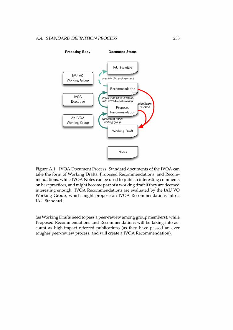
A.4. STANDARD DEFINITION PROCESS 235
Working Draft
Notes
significantrevision
IAU Standard
Recommendation
Proposed Recommendation
agreement withinworking group
IVOA-wide RFC, 4 weeks,with TCG 4-weeks review
possible IAU endorsementIAU VO
Working Group
IVOAExecutive
An IVOAWorking Group
Document StatusProposing Body
Figure A.1: IVOA Document Process. Standard documents of the IVOA cantake the form of Working Drafts, Proposed Recommendations, and Recom-mendations, while IVOA Notes can be used to publish interesting commentson best practices, and might become part of a working draft if they are deemedinteresting enough. IVOA Recommendations are evaluated by the IAU VOWorking Group, which might propose an IVOA Recommendations into aIAU Standard.
(as Working Drafts need to pass a peer-review among group members), whileProposed Recommendations and Recommendations will be taking into ac-count as high-impact refereed publications (as they have passed an evertougher peer-review process, and will create a IVOA Recommendation).

Appendix B
Introduction to XML
XML stands for eXtensible Markup Language. As the name implies, XML is acomputer language for the tagging —markup— of data, or more precisely, anspecification for writing particular markup languages. XML is Recommen-dation of the W3C since February 1998, and the latest XML 1.0 specificationcan be found at the W3C site1. For people not used to interpreting standardreferences, a solid reference guide to XML and related specifications is XMLin a nutshell [89].
The aim of this appendix is presenting astronomers, possibly with somedevelopment experience, with an introduction to XML, so that the VOTableappendix can be better understood.
B.1 Data markup
If we find the following set of data:
Juan de Dios Santander Vela23/05/1972Ingeniero en ElectrónicaInstituto de Astrofísica de Andalucía
we, as resourceful humans with lots of common sense, might think that thefirst line corresponds to the full name of a person, the second one is a date(most likely, a birth date), the third one is a degree (in Spanish), and the fourthone is an institution to which said person might belong.
A non-ambiguous way to present the information above could be thefollowing:
NAME: Juan de Dios Santander VelaBIRTHDATE: 23/05/1972DEGREE(es_ES): Ingeniero en ElectrónicaINSTITUTION: Instituto de Astrofísica de Andalucía
1http://www.w3.org/TR/REC-xml/
237
238 APPENDIX B. INTRODUCTION TO XML
That, for instance, is the kind of convention used in FITS header cards [9]:using keywords for particular pieces of data, and putting the data after saidkeywords.
However, that system brings its own share of problems. For instance, whatkind of keywords must be admitted? How many degrees can a person have,or how many institutions can that person belong to? If we wish to providethe same information for a large number of people, how does a computerrecognise the end of each record?
B.2 XML markup
In XML, those problems are solved by following these rules:
Tags enclose marked up data A piece of data is marked up by enclosing itbetween <TAG> and </TAG>. For instance, a person’s name would bea string enclosed between <NAME> and </NAME>, as in <NAME>Juan deDios Santander Vela</NAME> .
Tags are case sensitive In an XML document, all of the following are differenttags: <NAME>, <name>, <Name>. However, it is strongly recommendednot to use tags which only differ in their capitalisation.
At the root of an XML document, one and only one tag exists That means thatin XML documents, everything is inside a tag. If more tags need to bespecified, they must be enclosed in a higher hierarchy tag. With this inmind,
<NAME>Juan de Dios Santander Vela</NAME><BIRTHDATE>23/05/1972</BIRTHDATE>
is not a valid XML document, but
<PERSON><NAME>Juan de Dios Santander Vela</NAME><BIRTHDATE>23/05/1972</BIRTHDATE></PERSON>
is.
All tags reside completely within other tags This condition means that forclosing a tag, all other tags that might have opened inside must beclosed. That is, <strong><em>This is a text marked up with boldand italics </strong></em> is not valid XML, as the <em> tag opensafter the <strong> tag, but the <em> tag is still open when trying to close<strong>.
The last two conditions are also commonly stated as: XML documentsmust be well-formed. That is, well-formedness is the property of an XML
B.3. XML VALIDATION 239
document of having just a single root element, and having elementscompletely enclosed within other elements.
Additionally, XML tags can hold extra attributes. For instance, the<DEGREE>tag can have an language attribute which specifies the language and countryin which the degree was awarded, i.e., <DEGREE lang=‘es_ES’>Ingenieroen Electrónica</DEGREE> .
With those rules, the information above might be written in XML as:<PERSONS><PERSON><NAME>Juan de Dios Santander Vela</NAME><BIRTHDATE>23/05/1972</BIRTHDATE><DEGREE lang="es_ES">Ingeniero en Electrónica</DEGREE><INSTITUTION>Instituto de Astrofísica deAndalucía</INSTITUTION></PERSON></PERSONS>
An additional <PERSONS> tag has been included so that several <PERSON>records could be found in the same XML document.
B.3 XML validation
In the example above, we have devised an XML-based markup whose root ele-ment is the <PERSONS> tag, which can hold inside one or more <PERSON> tags,each one containing <NAME>, <BIRTHDATE>, <DEGREE> and <INSTITUTION>tags.
However, as there is been no specification of the language, how can acomputer make sure that the <INSTITUTION> tag belongs in the <PERSON>tag? What can be put inside a <BIRTHDATE> tag?
In other words, how can we specify a particular XML markup languageso that computers can validate particular XML document (instances) againstthat specification?
As originally XML was a subset of an existing markup language calledStandard Generalized Markup Language (SGML), XML documents used theSGML mechanism for markup specification, called Document Type Defini-tion (DTD). DTDs specify ELEMENTs, which are the particular tags which canappear in an XML document referencing the DTD, and ATTLISTs (attributelists), which are the sets of attributes that can modify a particular tag. TheELEMENT declarations’ syntax also allows for specifying which tags can occur,and how many times, inside others.
A DTD specifying the ELEMENTs and ATTLIST for the example above wouldbe:
240 APPENDIX B. INTRODUCTION TO XML
<!ELEMENT PERSONS (PERSON*)><!ELEMENT PERSON (NAME,BIRTHDATE?,DEGREE*,INSTITUTION*)><!ELEMENT NAME (#PCDATA)><!ELEMENT BIRTHDATE (#PCDATA)><!ELEMENT DEGREE (#PCDATA)><!ELEMENT INSTITUTION (#PCDATA)><!ATTLIST DEGREE lang CDATA #REQUIRED>
The rules for DTDs are:
• <!ELEMENT tag (tagcontents)> indicates that <tag> tags are allowed,with tagcontents inside.
• tagcontents is either a single tag, a list of tags separated by commas(,, indicating several tags which may appear in sequence), a list of tagsseparated by the vertical bar (|, indicating alternative tags which mightappear), the keyword ANY (indicating that any tag can occur inside), orthe keyword EMPTY (indicating that the <tag> tag must have no content,and can be used as <tag/>. All the tags appearing inside a tagcontentsmust have a corresponding <!ELEMENT tag> entry.
• The number of times a tag specified in tagcontents can appear dependson certain modifier characters after the tag. The asterisk (*) indicatesthat a tag can appear any number of times, including none at all. Thequestion mark (?) indicates that the tag is optional, and can appearonce or none at all. A plus sign (+) indicates that the tag must appear atleast once, but can appear many more times. If no symbol is specified,the tag appears just one time.
• <!ATTLIST tag attrName attrType defaultValue> specifies that the<tag> tag can have an attribute attrName. attrType is one of: CDATA(for strings); (a|b|...|n) (for an attribute which can be any one of ato n); ID (for a unique identifier); IDREF (for a reference to an ID of adifferent element); IDREFS (for a space-separated list of IDs to differentelements); and additional specifiers for entities and entity lists (entitiesare symbols representing particular characters or strings, such as &representing the ampersand (&)), shared controlled vocabularies (forattributes with the same list of possible values). And defaultValue iseither “value”, indicating the attrName can be set to any value, but ifnot value is applied by default; #IMPLIED for attributes which do notneed to be set, and for which no default value is assumed; #REQUIREDfor attributes which must be set with any value; or #FIXED “value” forattributes which must be set exactly to value.
If we take into account the rules above, our DTD states that:
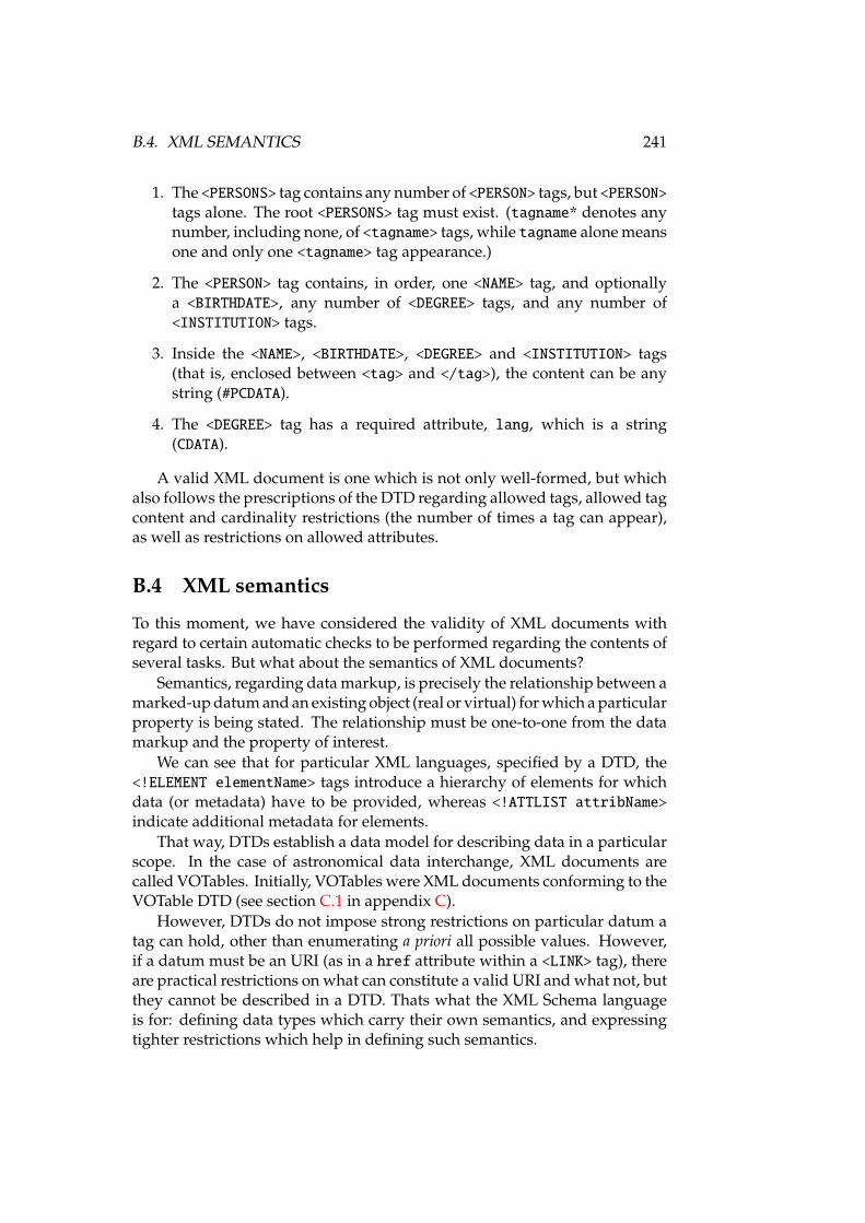
B.4. XML SEMANTICS 241
1. The <PERSONS> tag contains any number of <PERSON> tags, but <PERSON>tags alone. The root <PERSONS> tag must exist. (tagname* denotes anynumber, including none, of <tagname> tags, while tagname alone meansone and only one <tagname> tag appearance.)
2. The <PERSON> tag contains, in order, one <NAME> tag, and optionallya <BIRTHDATE>, any number of <DEGREE> tags, and any number of<INSTITUTION> tags.
3. Inside the <NAME>, <BIRTHDATE>, <DEGREE> and <INSTITUTION> tags(that is, enclosed between <tag> and </tag>), the content can be anystring (#PCDATA).
4. The <DEGREE> tag has a required attribute, lang, which is a string(CDATA).
A valid XML document is one which is not only well-formed, but whichalso follows the prescriptions of the DTD regarding allowed tags, allowed tagcontent and cardinality restrictions (the number of times a tag can appear),as well as restrictions on allowed attributes.
B.4 XML semantics
To this moment, we have considered the validity of XML documents withregard to certain automatic checks to be performed regarding the contents ofseveral tasks. But what about the semantics of XML documents?
Semantics, regarding data markup, is precisely the relationship between amarked-up datum and an existing object (real or virtual) for which a particularproperty is being stated. The relationship must be one-to-one from the datamarkup and the property of interest.
We can see that for particular XML languages, specified by a DTD, the<!ELEMENT elementName> tags introduce a hierarchy of elements for whichdata (or metadata) have to be provided, whereas <!ATTLIST attribName>indicate additional metadata for elements.
That way, DTDs establish a data model for describing data in a particularscope. In the case of astronomical data interchange, XML documents arecalled VOTables. Initially, VOTables were XML documents conforming to theVOTable DTD (see section C.1 in appendix C).
However, DTDs do not impose strong restrictions on particular datum atag can hold, other than enumerating a priori all possible values. However,if a datum must be an URI (as in a href attribute within a <LINK> tag), thereare practical restrictions on what can constitute a valid URI and what not, butthey cannot be described in a DTD. Thats what the XML Schema languageis for: defining data types which carry their own semantics, and expressingtighter restrictions which help in defining such semantics.
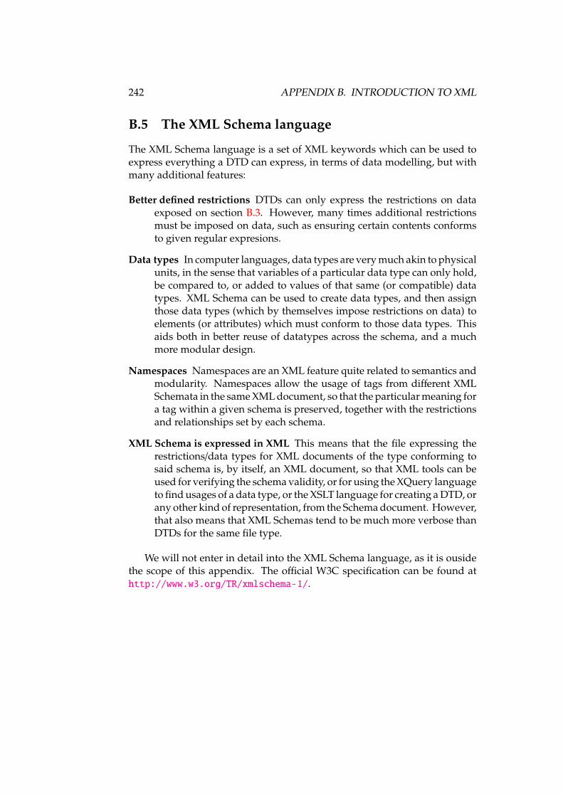
242 APPENDIX B. INTRODUCTION TO XML
B.5 The XML Schema language
The XML Schema language is a set of XML keywords which can be used toexpress everything a DTD can express, in terms of data modelling, but withmany additional features:
Better defined restrictions DTDs can only express the restrictions on dataexposed on section B.3. However, many times additional restrictionsmust be imposed on data, such as ensuring certain contents conformsto given regular expresions.
Data types In computer languages, data types are very much akin to physicalunits, in the sense that variables of a particular data type can only hold,be compared to, or added to values of that same (or compatible) datatypes. XML Schema can be used to create data types, and then assignthose data types (which by themselves impose restrictions on data) toelements (or attributes) which must conform to those data types. Thisaids both in better reuse of datatypes across the schema, and a muchmore modular design.
Namespaces Namespaces are an XML feature quite related to semantics andmodularity. Namespaces allow the usage of tags from different XMLSchemata in the same XML document, so that the particular meaning fora tag within a given schema is preserved, together with the restrictionsand relationships set by each schema.
XML Schema is expressed in XML This means that the file expressing therestrictions/data types for XML documents of the type conforming tosaid schema is, by itself, an XML document, so that XML tools can beused for verifying the schema validity, or for using the XQuery languageto find usages of a data type, or the XSLT language for creating a DTD, orany other kind of representation, from the Schema document. However,that also means that XML Schemas tend to be much more verbose thanDTDs for the same file type.
We will not enter in detail into the XML Schema language, as it is ousidethe scope of this appendix. The official W3C specification can be found athttp://www.w3.org/TR/xmlschema-1/.
Appendix C
VOTable format definition
The VOTable is the main data interchange standard existing in the VO, andis an IVOA Recommendation since 2004. Its formal definition can be foundin [86], or in the IVOA Documents site1. However, we will provide in this ap-pendix a brief description of the VOTable format which also aims to illustratesome parts of that document.
C.1 VOTable DTD
The initial definition of the VOTable, version 1.0, was made in terms of anXML Document Type Definition (DTD), which can be found in listing C.1.This document specifies ELEMENTs, which are the tags that can be used tomarkup data, and which tags can be included, and how many times, withinany other tag; and ATTLISTs, or attribute lists, which are the attributes thatcan further refine a tag being applied to a piece of data.
C.2 VOTable XML Schema Definition
A new version of the VOTable, version 1.1, was a little bit more restrictiveon what is an acceptable VOTable, by means of an XML Schema Definition(XSD). The XML schema can be seen in listing C.4.
C.3 VOTable structure
Independently of whether a VOTable XML document specifies its documenttype via a DTD or the VOTable XML Schena, its structure can be seen infigure C.1.
A VOTable, then, is an XML document whose root element is the<VOTABLE>tag, and which might hold inside a <DESCRIPTION> tag, a <DEFINITIONS>
1http://www.ivoa.net/Documents/latest/VOT.html
243
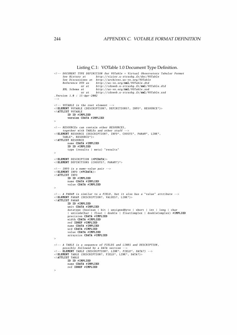
244 APPENDIX C. VOTABLE FORMAT DEFINITION
Listing C.1: VOTable 1.0 Document Type Definition.<!-- DOCUMENT TYPE DEFINITION for VOTable = Virtual Observatory Tabular Format
See History at http://vizier.u-strasbg.fr/doc/VOTableSee Discussions at http://archives.us-vo.org/VOTableReference DTD as http://us-vo.org/xml/VOTable.dtd
or at http://cdsweb.u-strasbg.fr/xml/VOTable.dtdXML Schema at http://us-vo.org/xml/VOTable.xsd
or at http://cdsweb.u-strasbg.fr/xml/VOTable.xsd.Version 1.0 : 15-Apr-2002-->
<!-- VOTABLE is the root element --><!ELEMENT VOTABLE (DESCRIPTION?, DEFINITIONS?, INFO*, RESOURCE*)><!ATTLIST VOTABLE
ID ID #IMPLIEDversion CDATA #IMPLIED
>
<!-- RESOURCEs can contain other RESOURCES ,together with TABLEs and other stuff -->
<!ELEMENT RESOURCE (DESCRIPTION?, INFO*, COOSYS*, PARAM*, LINK*,TABLE*, RESOURCE*)>
<!ATTLIST RESOURCEname CDATA #IMPLIEDID ID #IMPLIEDtype (results | meta) "results"
>
<!ELEMENT DESCRIPTION (#PCDATA)><!ELEMENT DEFINITIONS (COOSYS?, PARAM?)*>
<!-- INFO is a name-value pair --><!ELEMENT INFO (#PCDATA)><!ATTLIST INFO
ID ID #IMPLIEDname CDATA #IMPLIEDvalue CDATA #IMPLIED
>
<!-- A PARAM is similar to a FIELD, but it also has a "value" attribute --><!ELEMENT PARAM (DESCRIPTION?, VALUES?, LINK*)><!ATTLIST PARAM
ID ID #IMPLIEDunit CDATA #IMPLIEDdatatype (boolean | bit | unsignedByte | short | int | long | char| unicodeChar | float | double | floatComplex | doubleComplex) #IMPLIEDprecision CDATA #IMPLIEDwidth CDATA #IMPLIEDref IDREF #IMPLIEDname CDATA #IMPLIEDucd CDATA #IMPLIEDvalue CDATA #IMPLIEDarraysize CDATA #IMPLIED
>
<!-- A TABLE is a sequence of FIELDS and LINKS and DESCRIPTION ,possibly followed by a DATA section -->
<!-- ELEMENT TABLE (DESCRIPTION?, LINK*, FIELD*, DATA?) --><!ELEMENT TABLE (DESCRIPTION?, FIELD*, LINK*, DATA?)><!ATTLIST TABLE
ID ID #IMPLIEDname CDATA #IMPLIEDref IDREF #IMPLIED
>
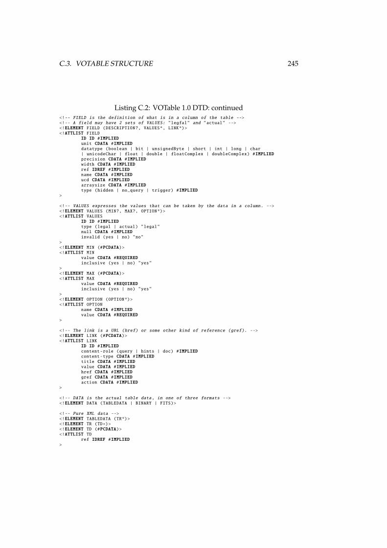
C.3. VOTABLE STRUCTURE 245
Listing C.2: VOTable 1.0 DTD: continued<!-- FIELD is the definition of what is in a column of the table --><!-- A field may have 2 sets of VALUES: "legfal" and "actual" --><!ELEMENT FIELD (DESCRIPTION?, VALUES*, LINK*)><!ATTLIST FIELD
ID ID #IMPLIEDunit CDATA #IMPLIEDdatatype (boolean | bit | unsignedByte | short | int | long | char| unicodeChar | float | double | floatComplex | doubleComplex) #IMPLIEDprecision CDATA #IMPLIEDwidth CDATA #IMPLIEDref IDREF #IMPLIEDname CDATA #IMPLIEDucd CDATA #IMPLIEDarraysize CDATA #IMPLIEDtype (hidden | no_query | trigger) #IMPLIED
>
<!-- VALUES expresses the values that can be taken by the data in a column. --><!ELEMENT VALUES (MIN?, MAX?, OPTION*)><!ATTLIST VALUES
ID ID #IMPLIEDtype (legal | actual) "legal"null CDATA #IMPLIEDinvalid (yes | no) "no"
><!ELEMENT MIN (#PCDATA)><!ATTLIST MIN
value CDATA #REQUIREDinclusive (yes | no) "yes"
><!ELEMENT MAX (#PCDATA)><!ATTLIST MAX
value CDATA #REQUIREDinclusive (yes | no) "yes"
><!ELEMENT OPTION (OPTION*)><!ATTLIST OPTION
name CDATA #IMPLIEDvalue CDATA #REQUIRED
>
<!-- The link is a URL (href) or some other kind of reference (gref). --><!ELEMENT LINK (#PCDATA)><!ATTLIST LINK
ID ID #IMPLIEDcontent-role (query | hints | doc) #IMPLIEDcontent-type CDATA #IMPLIEDtitle CDATA #IMPLIEDvalue CDATA #IMPLIEDhref CDATA #IMPLIEDgref CDATA #IMPLIEDaction CDATA #IMPLIED
>
<!-- DATA is the actual table data, in one of three formats --><!ELEMENT DATA (TABLEDATA | BINARY | FITS)>
<!-- Pure XML data --><!ELEMENT TABLEDATA (TR*)><!ELEMENT TR (TD+)><!ELEMENT TD (#PCDATA)><!ATTLIST TD
ref IDREF #IMPLIED>
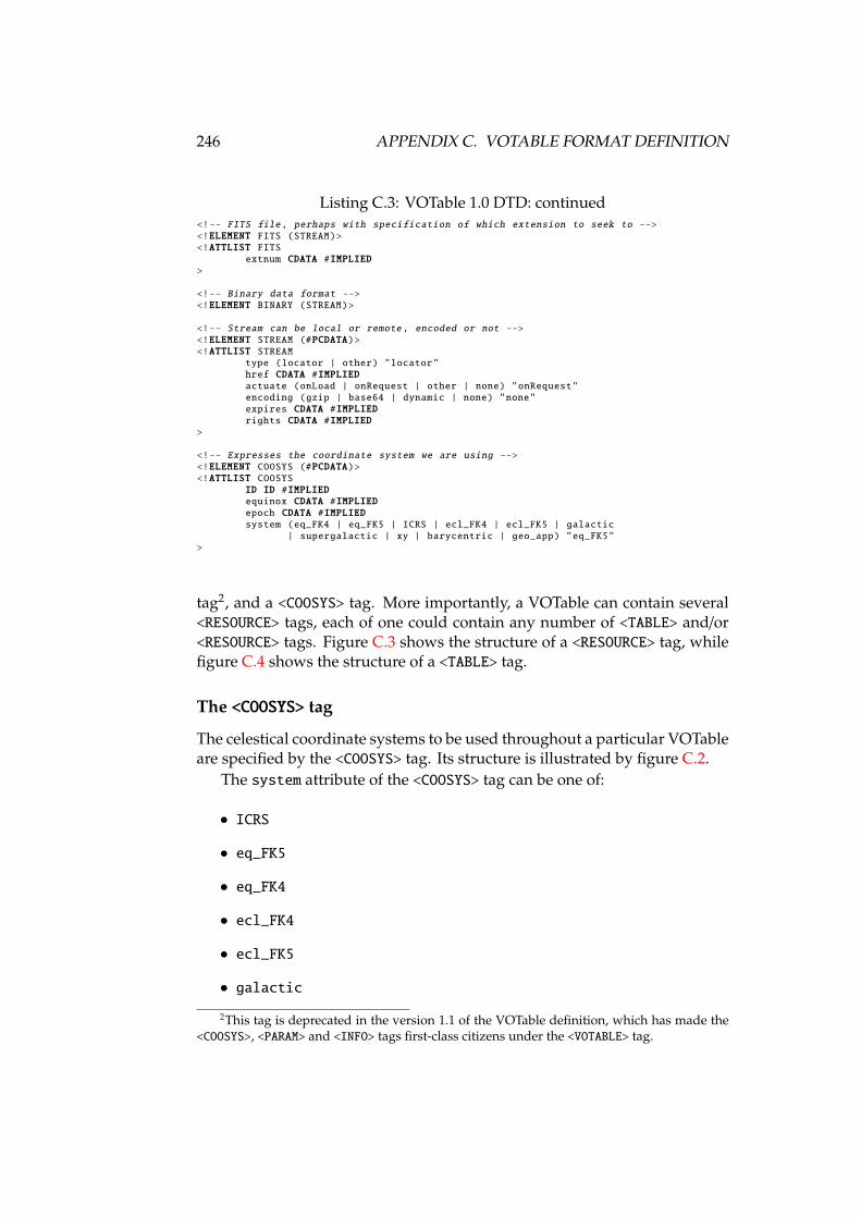
246 APPENDIX C. VOTABLE FORMAT DEFINITION
Listing C.3: VOTable 1.0 DTD: continued<!-- FITS file, perhaps with specification of which extension to seek to --><!ELEMENT FITS (STREAM)><!ATTLIST FITS
extnum CDATA #IMPLIED>
<!-- Binary data format --><!ELEMENT BINARY (STREAM)>
<!-- Stream can be local or remote, encoded or not --><!ELEMENT STREAM (#PCDATA)><!ATTLIST STREAM
type (locator | other) "locator"href CDATA #IMPLIEDactuate (onLoad | onRequest | other | none) "onRequest"encoding (gzip | base64 | dynamic | none) "none"expires CDATA #IMPLIEDrights CDATA #IMPLIED
>
<!-- Expresses the coordinate system we are using --><!ELEMENT COOSYS (#PCDATA)><!ATTLIST COOSYS
ID ID #IMPLIEDequinox CDATA #IMPLIEDepoch CDATA #IMPLIEDsystem (eq_FK4 | eq_FK5 | ICRS | ecl_FK4 | ecl_FK5 | galactic
| supergalactic | xy | barycentric | geo_app) "eq_FK5">
tag2, and a <COOSYS> tag. More importantly, a VOTable can contain several<RESOURCE> tags, each of one could contain any number of <TABLE> and/or<RESOURCE> tags. Figure C.3 shows the structure of a <RESOURCE> tag, whilefigure C.4 shows the structure of a <TABLE> tag.
The <COOSYS> tag
The celestical coordinate systems to be used throughout a particular VOTableare specified by the <COOSYS> tag. Its structure is illustrated by figure C.2.
The system attribute of the <COOSYS> tag can be one of:
• ICRS
• eq_FK5
• eq_FK4
• ecl_FK4
• ecl_FK5
• galactic
2This tag is deprecated in the version 1.1 of the VOTable definition, which has made the<COOSYS>, <PARAM> and <INFO> tags first-class citizens under the <VOTABLE> tag.
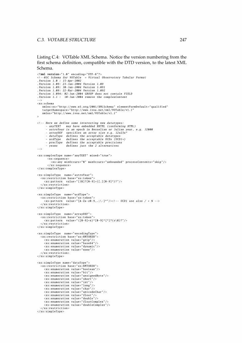
C.3. VOTABLE STRUCTURE 247
Listing C.4: VOTable XML Schema. Notice the version numbering from thefirst schema definition, compatible with the DTD version, to the latest XMLSchema.<?xml version="1.0" encoding="UTF-8"?><!--W3C Schema for VOTable = Virtual Observatory Tabular Format.Version 1.0 : 15-Apr-2002.Version 1.09: 23-Jan-2004 Version 1.09.Version 1.09: 30-Jan-2004 Version 1.091.Version 1.09: 22-Mar-2004 Version 1.092.Version 1.094: 02-Jun-2004 GROUP does not contain FIELD.Version 1.1 : 10-Jun-2004 remove the complexContent--><xs:schema
xmlns:xs="http://www.w3.org/2001/XMLSchema" elementFormDefault="qualified"targetNamespace="http://www.ivoa.net/xml/VOTable/v1.1"xmlns="http://www.ivoa.net/xml/VOTable/v1.1"
>
<!-- Here we define some interesting new datatypes:- anyTEXT may have embedded XHTML (conforming HTML)- astroYear is an epoch in Besselian or Julian year, e.g. J2000- arrayDEF specifies an array size e.g. 12x23x*- dataType defines the acceptable datatypes- ucdType defines the acceptable UCDs (UCD1+)- precType defines the acceptable precisions- yesno defines just the 2 alternatives
-->
<xs:complexType name="anyTEXT" mixed="true"><xs:sequence>
<xs:any minOccurs="0" maxOccurs="unbounded" processContents="skip"/></xs:sequence>
</xs:complexType>
<xs:simpleType name="astroYear"><xs:restriction base="xs:token">
<xs:pattern value="[JB]?[0-9]+([.][0-9]*)?"/></xs:restriction>
</xs:simpleType>
<xs:simpleType name="ucdType"><xs:restriction base="xs:token">
<xs:pattern value="[A-Za-z0-9_.;\-]*"/><!-- UCD1 use also / + % --></xs:restriction>
</xs:simpleType>
<xs:simpleType name="arrayDEF"><xs:restriction base="xs:token">
<xs:pattern value="([0-9]+x)*[0-9]*[*]?(s\W)?"/></xs:restriction>
</xs:simpleType>
<xs:simpleType name="encodingType"><xs:restriction base="xs:NMTOKEN">
<xs:enumeration value="gzip"/><xs:enumeration value="base64"/><xs:enumeration value="dynamic"/><xs:enumeration value="none"/>
</xs:restriction></xs:simpleType>
<xs:simpleType name="dataType"><xs:restriction base="xs:NMTOKEN">
<xs:enumeration value="boolean"/><xs:enumeration value="bit"/><xs:enumeration value="unsignedByte"/><xs:enumeration value="short"/><xs:enumeration value="int"/><xs:enumeration value="long"/><xs:enumeration value="char"/><xs:enumeration value="unicodeChar"/><xs:enumeration value="float"/><xs:enumeration value="double"/><xs:enumeration value="floatComplex"/><xs:enumeration value="doubleComplex"/>
</xs:restriction></xs:simpleType>
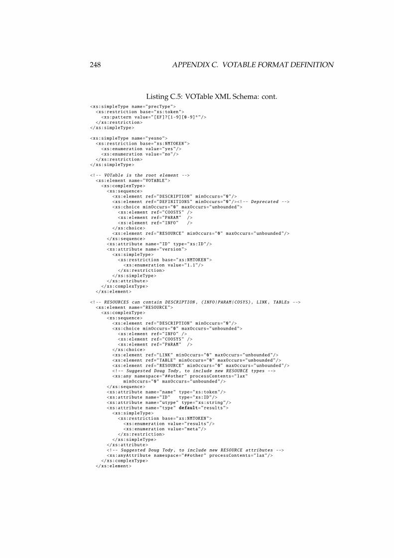
248 APPENDIX C. VOTABLE FORMAT DEFINITION
Listing C.5: VOTable XML Schema: cont.<xs:simpleType name="precType">
<xs:restriction base="xs:token"><xs:pattern value="[EF]?[1-9][0-9]*"/>
</xs:restriction></xs:simpleType>
<xs:simpleType name="yesno"><xs:restriction base="xs:NMTOKEN">
<xs:enumeration value="yes"/><xs:enumeration value="no"/>
</xs:restriction></xs:simpleType>
<!-- VOTable is the root element --><xs:element name="VOTABLE">
<xs:complexType><xs:sequence>
<xs:element ref="DESCRIPTION" minOccurs="0"/><xs:element ref="DEFINITIONS" minOccurs="0"/><!-- Deprecated --><xs:choice minOccurs="0" maxOccurs="unbounded">
<xs:element ref="COOSYS" /><xs:element ref="PARAM" /><xs:element ref="INFO" />
</xs:choice><xs:element ref="RESOURCE" minOccurs="0" maxOccurs="unbounded"/>
</xs:sequence><xs:attribute name="ID" type="xs:ID"/><xs:attribute name="version">
<xs:simpleType><xs:restriction base="xs:NMTOKEN">
<xs:enumeration value="1.1"/></xs:restriction>
</xs:simpleType></xs:attribute>
</xs:complexType></xs:element>
<!-- RESOURCES can contain DESCRIPTION , (INFO|PARAM|COSYS), LINK, TABLEs --><xs:element name="RESOURCE">
<xs:complexType><xs:sequence>
<xs:element ref="DESCRIPTION" minOccurs="0"/><xs:choice minOccurs="0" maxOccurs="unbounded">
<xs:element ref="INFO" /><xs:element ref="COOSYS" /><xs:element ref="PARAM" />
</xs:choice><xs:element ref="LINK" minOccurs="0" maxOccurs="unbounded"/><xs:element ref="TABLE" minOccurs="0" maxOccurs="unbounded"/><xs:element ref="RESOURCE" minOccurs="0" maxOccurs="unbounded"/><!-- Suggested Doug Tody, to include new RESOURCE types --><xs:any namespace="##other" processContents="lax"
minOccurs="0" maxOccurs="unbounded"/></xs:sequence><xs:attribute name="name" type="xs:token"/><xs:attribute name="ID" type="xs:ID"/><xs:attribute name="utype" type="xs:string"/><xs:attribute name="type" default="results">
<xs:simpleType><xs:restriction base="xs:NMTOKEN">
<xs:enumeration value="results"/><xs:enumeration value="meta"/>
</xs:restriction></xs:simpleType>
</xs:attribute><!-- Suggested Doug Tody, to include new RESOURCE attributes --><xs:anyAttribute namespace="##other" processContents="lax"/>
</xs:complexType></xs:element>
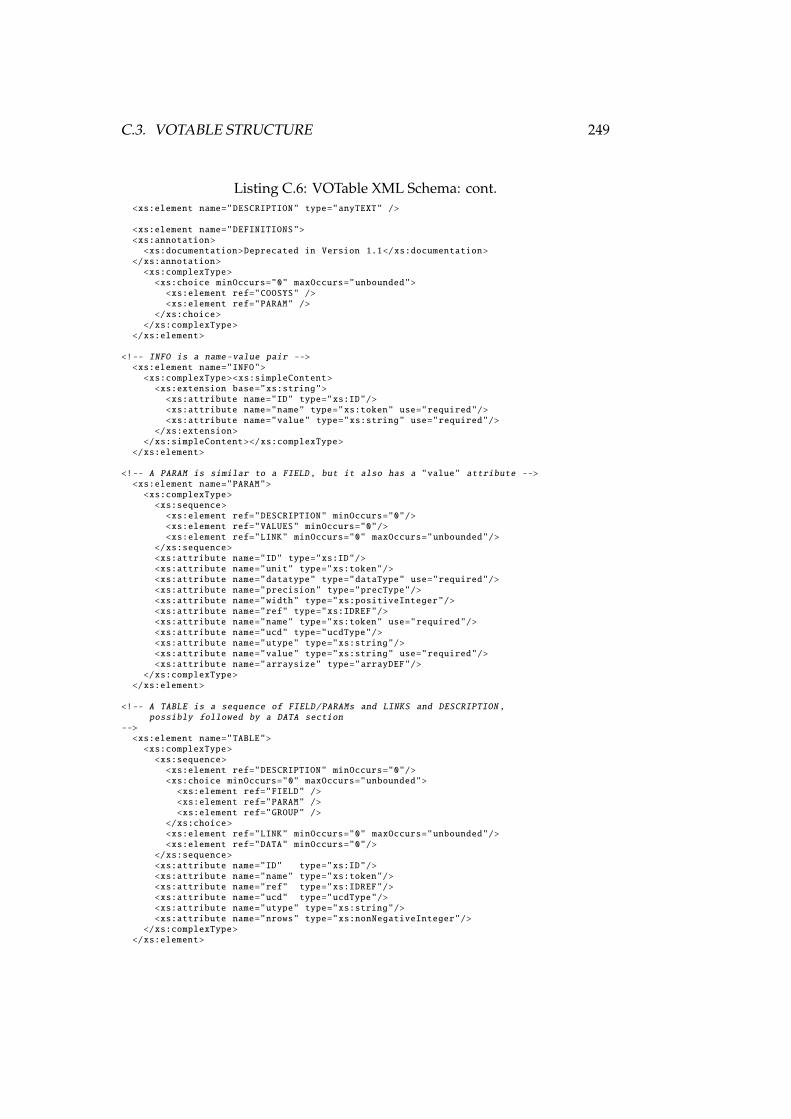
C.3. VOTABLE STRUCTURE 249
Listing C.6: VOTable XML Schema: cont.<xs:element name="DESCRIPTION" type="anyTEXT" />
<xs:element name="DEFINITIONS"><xs:annotation>
<xs:documentation>Deprecated in Version 1.1</xs:documentation></xs:annotation>
<xs:complexType><xs:choice minOccurs="0" maxOccurs="unbounded">
<xs:element ref="COOSYS" /><xs:element ref="PARAM" />
</xs:choice></xs:complexType>
</xs:element>
<!-- INFO is a name-value pair --><xs:element name="INFO">
<xs:complexType><xs:simpleContent><xs:extension base="xs:string">
<xs:attribute name="ID" type="xs:ID"/><xs:attribute name="name" type="xs:token" use="required"/><xs:attribute name="value" type="xs:string" use="required"/>
</xs:extension></xs:simpleContent></xs:complexType>
</xs:element>
<!-- A PARAM is similar to a FIELD, but it also has a "value" attribute --><xs:element name="PARAM">
<xs:complexType><xs:sequence>
<xs:element ref="DESCRIPTION" minOccurs="0"/><xs:element ref="VALUES" minOccurs="0"/><xs:element ref="LINK" minOccurs="0" maxOccurs="unbounded"/>
</xs:sequence><xs:attribute name="ID" type="xs:ID"/><xs:attribute name="unit" type="xs:token"/><xs:attribute name="datatype" type="dataType" use="required"/><xs:attribute name="precision" type="precType"/><xs:attribute name="width" type="xs:positiveInteger"/><xs:attribute name="ref" type="xs:IDREF"/><xs:attribute name="name" type="xs:token" use="required"/><xs:attribute name="ucd" type="ucdType"/><xs:attribute name="utype" type="xs:string"/><xs:attribute name="value" type="xs:string" use="required"/><xs:attribute name="arraysize" type="arrayDEF"/>
</xs:complexType></xs:element>
<!-- A TABLE is a sequence of FIELD/PARAMs and LINKS and DESCRIPTION ,possibly followed by a DATA section
--><xs:element name="TABLE">
<xs:complexType><xs:sequence>
<xs:element ref="DESCRIPTION" minOccurs="0"/><xs:choice minOccurs="0" maxOccurs="unbounded">
<xs:element ref="FIELD" /><xs:element ref="PARAM" /><xs:element ref="GROUP" />
</xs:choice><xs:element ref="LINK" minOccurs="0" maxOccurs="unbounded"/><xs:element ref="DATA" minOccurs="0"/>
</xs:sequence><xs:attribute name="ID" type="xs:ID"/><xs:attribute name="name" type="xs:token"/><xs:attribute name="ref" type="xs:IDREF"/><xs:attribute name="ucd" type="ucdType"/><xs:attribute name="utype" type="xs:string"/><xs:attribute name="nrows" type="xs:nonNegativeInteger"/>
</xs:complexType></xs:element>

250 APPENDIX C. VOTABLE FORMAT DEFINITION
Listing C.7: VOTable XML Schema: cont.
<!-- FIELD is the definition of what is in a column of the table --><xs:element name="FIELD">
<xs:complexType><xs:sequence> <!-- minOccurs="0" maxOccurs="unbounded" -->
<xs:element ref="DESCRIPTION" minOccurs="0"/><xs:element ref="VALUES" minOccurs="0"/> <!-- maxOccurs="2" --><xs:element ref="LINK" minOccurs="0" maxOccurs="unbounded"/>
</xs:sequence><xs:attribute name="ID" type="xs:ID"/><xs:attribute name="unit" type="xs:token"/><xs:attribute name="datatype" type="dataType" use="required"/><xs:attribute name="precision" type="precType"/><xs:attribute name="width" type="xs:positiveInteger"/><xs:attribute name="ref" type="xs:IDREF"/><xs:attribute name="name" type="xs:token" use="required"/><xs:attribute name="ucd" type="ucdType"/><xs:attribute name="utype" type="xs:string"/><xs:attribute name="arraysize" type="xs:string"/><xs:attribute name="type">
<!-- type is not in the Version 1.1, but is kept forbackward compatibility purposes
--><xs:simpleType>
<xs:restriction base="xs:NMTOKEN"><xs:enumeration value="hidden"/><xs:enumeration value="no_query"/><xs:enumeration value="trigger"/><xs:enumeration value="location"/>
</xs:restriction></xs:simpleType>
</xs:attribute></xs:complexType>
</xs:element>
<!-- GROUP groups columns; may include descriptions , fields/params/groups --><xs:element name="GROUP">
<xs:complexType><xs:sequence>
<xs:element ref="DESCRIPTION" minOccurs="0"/><xs:choice minOccurs="0" maxOccurs="unbounded">
<xs:element ref="FIELDref"/><xs:element ref="PARAMref"/><xs:element ref="PARAM"/><xs:element ref="GROUP"/>
</xs:choice></xs:sequence><xs:attribute name="ID" type="xs:ID"/><xs:attribute name="name" type="xs:token"/><xs:attribute name="ref" type="xs:IDREF"/><xs:attribute name="ucd" type="ucdType"/><xs:attribute name="utype" type="xs:string"/>
</xs:complexType></xs:element>
<!-- FIELDref and PARAMref are references to FIELD or PARAM definedin the parent TABLE or RESOURCE -->
<xs:element name="FIELDref"><xs:complexType>
<xs:attribute name="ref" type="xs:IDREF" use="required"/><!-- utype and maybe ucd could well be added there,
will be if necessary --></xs:complexType>
</xs:element><xs:element name="PARAMref">
<xs:complexType><xs:attribute name="ref" type="xs:IDREF" use="required"/><!-- utype and maybe ucd could well be added there,
will be if necessary --></xs:complexType>
</xs:element>
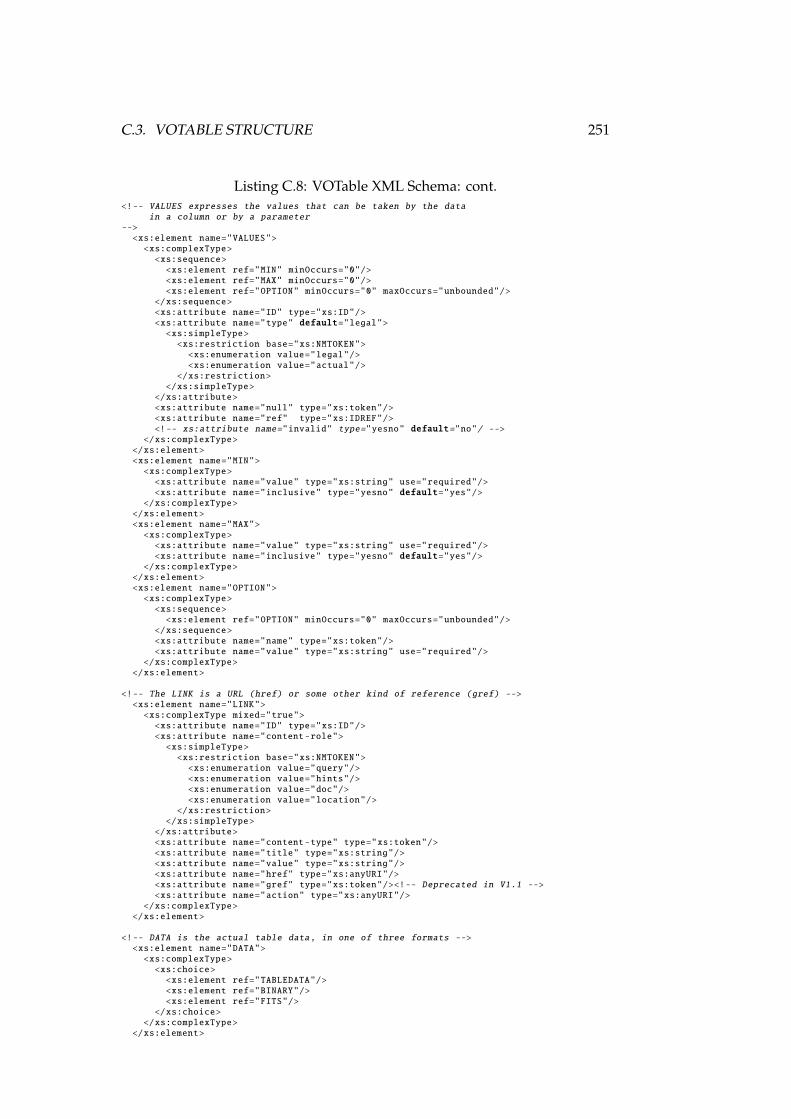
C.3. VOTABLE STRUCTURE 251
Listing C.8: VOTable XML Schema: cont.<!-- VALUES expresses the values that can be taken by the data
in a column or by a parameter-->
<xs:element name="VALUES"><xs:complexType>
<xs:sequence><xs:element ref="MIN" minOccurs="0"/><xs:element ref="MAX" minOccurs="0"/><xs:element ref="OPTION" minOccurs="0" maxOccurs="unbounded"/>
</xs:sequence><xs:attribute name="ID" type="xs:ID"/><xs:attribute name="type" default="legal">
<xs:simpleType><xs:restriction base="xs:NMTOKEN">
<xs:enumeration value="legal"/><xs:enumeration value="actual"/>
</xs:restriction></xs:simpleType>
</xs:attribute><xs:attribute name="null" type="xs:token"/><xs:attribute name="ref" type="xs:IDREF"/><!-- xs:attribute name="invalid" type="yesno" default="no"/ -->
</xs:complexType></xs:element><xs:element name="MIN">
<xs:complexType><xs:attribute name="value" type="xs:string" use="required"/><xs:attribute name="inclusive" type="yesno" default="yes"/>
</xs:complexType></xs:element><xs:element name="MAX">
<xs:complexType><xs:attribute name="value" type="xs:string" use="required"/><xs:attribute name="inclusive" type="yesno" default="yes"/>
</xs:complexType></xs:element><xs:element name="OPTION">
<xs:complexType><xs:sequence>
<xs:element ref="OPTION" minOccurs="0" maxOccurs="unbounded"/></xs:sequence><xs:attribute name="name" type="xs:token"/><xs:attribute name="value" type="xs:string" use="required"/>
</xs:complexType></xs:element>
<!-- The LINK is a URL (href) or some other kind of reference (gref) --><xs:element name="LINK">
<xs:complexType mixed="true"><xs:attribute name="ID" type="xs:ID"/><xs:attribute name="content-role">
<xs:simpleType><xs:restriction base="xs:NMTOKEN">
<xs:enumeration value="query"/><xs:enumeration value="hints"/><xs:enumeration value="doc"/><xs:enumeration value="location"/>
</xs:restriction></xs:simpleType>
</xs:attribute><xs:attribute name="content-type" type="xs:token"/><xs:attribute name="title" type="xs:string"/><xs:attribute name="value" type="xs:string"/><xs:attribute name="href" type="xs:anyURI"/><xs:attribute name="gref" type="xs:token"/><!-- Deprecated in V1.1 --><xs:attribute name="action" type="xs:anyURI"/>
</xs:complexType></xs:element>
<!-- DATA is the actual table data, in one of three formats --><xs:element name="DATA">
<xs:complexType><xs:choice>
<xs:element ref="TABLEDATA"/><xs:element ref="BINARY"/><xs:element ref="FITS"/>
</xs:choice></xs:complexType>
</xs:element>
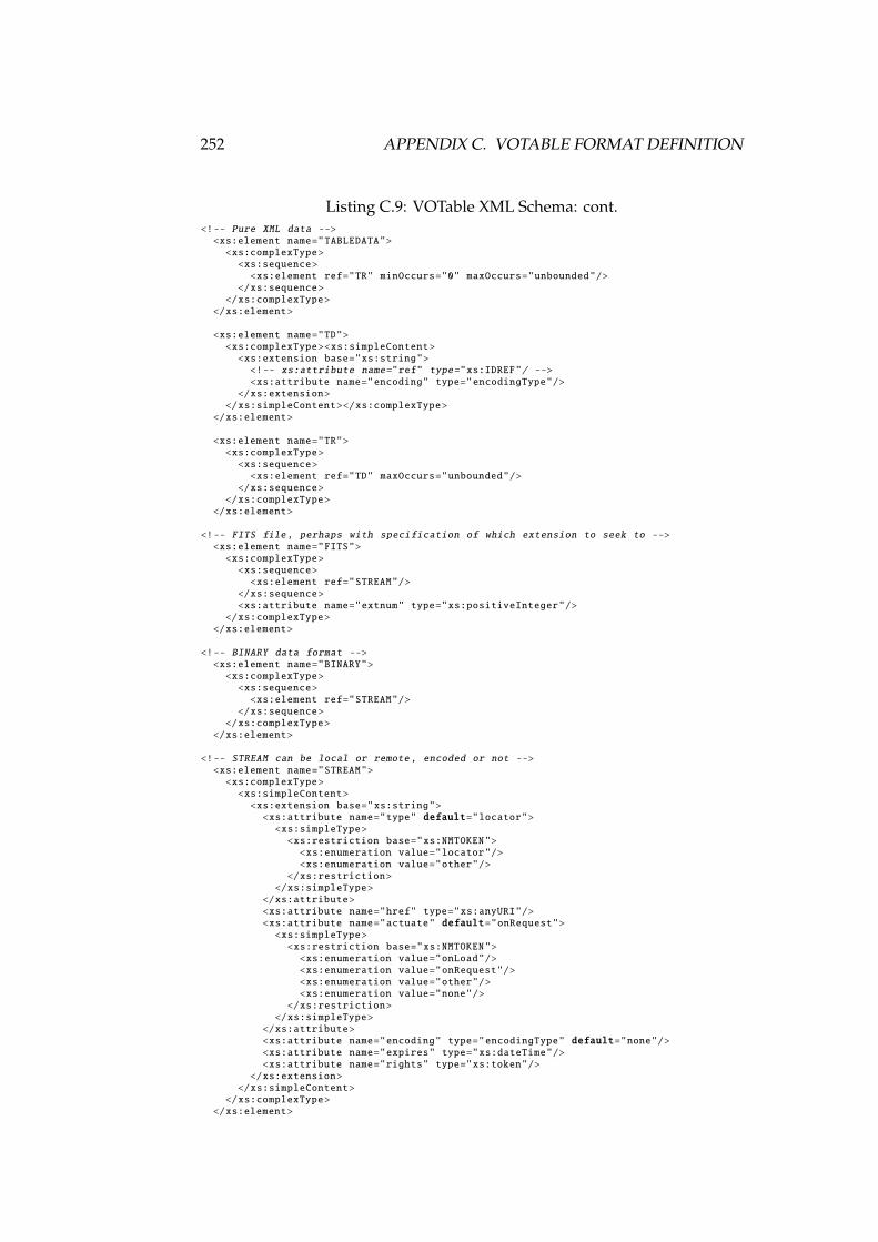
252 APPENDIX C. VOTABLE FORMAT DEFINITION
Listing C.9: VOTable XML Schema: cont.<!-- Pure XML data -->
<xs:element name="TABLEDATA"><xs:complexType>
<xs:sequence><xs:element ref="TR" minOccurs="0" maxOccurs="unbounded"/>
</xs:sequence></xs:complexType>
</xs:element>
<xs:element name="TD"><xs:complexType><xs:simpleContent>
<xs:extension base="xs:string"><!-- xs:attribute name="ref" type="xs:IDREF"/ --><xs:attribute name="encoding" type="encodingType"/>
</xs:extension></xs:simpleContent></xs:complexType>
</xs:element>
<xs:element name="TR"><xs:complexType>
<xs:sequence><xs:element ref="TD" maxOccurs="unbounded"/>
</xs:sequence></xs:complexType>
</xs:element>
<!-- FITS file, perhaps with specification of which extension to seek to --><xs:element name="FITS">
<xs:complexType><xs:sequence>
<xs:element ref="STREAM"/></xs:sequence><xs:attribute name="extnum" type="xs:positiveInteger"/>
</xs:complexType></xs:element>
<!-- BINARY data format --><xs:element name="BINARY">
<xs:complexType><xs:sequence>
<xs:element ref="STREAM"/></xs:sequence>
</xs:complexType></xs:element>
<!-- STREAM can be local or remote, encoded or not --><xs:element name="STREAM">
<xs:complexType><xs:simpleContent>
<xs:extension base="xs:string"><xs:attribute name="type" default="locator">
<xs:simpleType><xs:restriction base="xs:NMTOKEN">
<xs:enumeration value="locator"/><xs:enumeration value="other"/>
</xs:restriction></xs:simpleType>
</xs:attribute><xs:attribute name="href" type="xs:anyURI"/><xs:attribute name="actuate" default="onRequest">
<xs:simpleType><xs:restriction base="xs:NMTOKEN">
<xs:enumeration value="onLoad"/><xs:enumeration value="onRequest"/><xs:enumeration value="other"/><xs:enumeration value="none"/>
</xs:restriction></xs:simpleType>
</xs:attribute><xs:attribute name="encoding" type="encodingType" default="none"/><xs:attribute name="expires" type="xs:dateTime"/><xs:attribute name="rights" type="xs:token"/>
</xs:extension></xs:simpleContent>
</xs:complexType></xs:element>
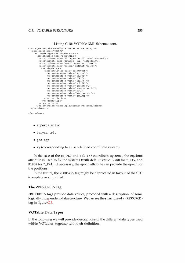
C.3. VOTABLE STRUCTURE 253
Listing C.10: VOTable XML Schema: cont.<!-- Expresses the coordinate system we are using -->
<xs:element name="COOSYS"><xs:complexType><xs:simpleContent>
<xs:extension base="xs:string"><xs:attribute name="ID" type="xs:ID" use="required"/><xs:attribute name="equinox" type="astroYear"/><xs:attribute name="epoch" type="astroYear"/><xs:attribute name="system" default="eq_FK5">
<xs:simpleType><xs:restriction base="xs:NMTOKEN">
<xs:enumeration value="eq_FK4"/><xs:enumeration value="eq_FK5"/><xs:enumeration value="ICRS"/><xs:enumeration value="ecl_FK4"/><xs:enumeration value="ecl_FK5"/><xs:enumeration value="galactic"/><xs:enumeration value="supergalactic"/><xs:enumeration value="xy"/><xs:enumeration value="barycentric"/><xs:enumeration value="geo_app"/>
</xs:restriction></xs:simpleType>
</xs:attribute></xs:extension></xs:simpleContent></xs:complexType>
</xs:element>
</xs:schema>
• supergalactic
• barycentric
• geo_app
• xy (corresponding to a user-defined coordinate system)
In the case of the eq_FK? and ecl_FK? coordinate systems, the equinoxattribute is used to fix the systems (with default vaule J2000 for *_FK5, andB1950 for *_FK4). If necessary, the epoch attribute can provide the epoch forthe positions.
In the future, the <COOSYS> tag might be deprecated in favour of the STC(complete or simplified).
The <RESOURCE> tag
<RESOURCE> tags provide data values, preceded with a description, of somelogically independent data structure. We can see the structure of a<RESOURCE>tag in figure C.3.
VOTable Data Types
In the following we will provide descriptions of the different data types usedwithin VOTables, together with their definition.
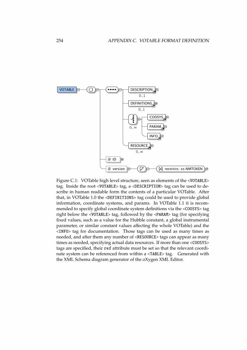
254 APPENDIX C. VOTABLE FORMAT DEFINITION
VOTABLE DESCRIPTION
0..1
DEFINITIONS
0..1
0..
COOSYS
PARAM
INFO
RESOURCE
0..
@ ID
@ version restricts: xs:NMTOKEN
Figure C.1: VOTable high level structure, seen as elements of the <VOTABLE>tag. Inside the root <VOTABLE> tag, a <DESCRIPTION> tag can be used to de-scribe in human readable form the contents of a particular VOTable. Afterthat, in VOTable 1.0 the <DEFINITIONS> tag could be used to provide globalinformation, coordinate systems, and params. In VOTable 1.1 it is recom-mended to specify global coordinate system definitions via the <COOSYS> tagright below the <VOTABLE> tag, followed by the <PARAM> tag (for specifyingfixed values, such as a value for the Hubble constant, a global instrumentalparameter, or similar constant values affecting the whole VOTable) and the<INFO> tag for documentation. Those tags can be used as many times asneeded, and after them any number of <RESOURCE> tags can appear as manytimes as needed, specifying actual data resources. If more than one <COOSYS>tags are specified, their ref attribute must be set so that the relevant coordi-nate system can be referenced from within a <TABLE> tag. Generated withthe XML Schema diagram generator of the oXygen XML Editor.
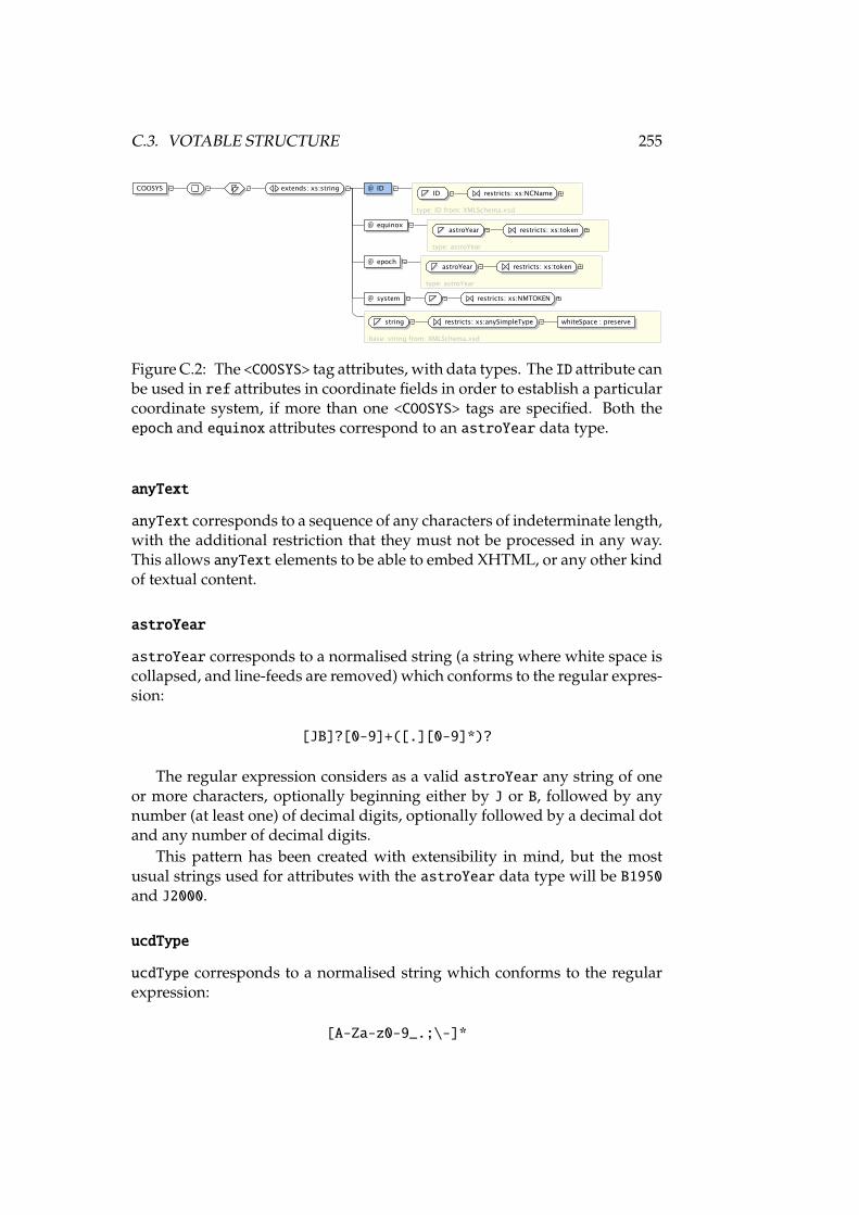
C.3. VOTABLE STRUCTURE 255
COOSYS extends: xs:string @ ID
type: ID from: XMLSchema.xsd
ID restricts: xs:NCName
@ equinox
type: astroYear
astroYear restricts: xs:token
@ epoch
type: astroYear
astroYear restricts: xs:token
@ system restricts: xs:NMTOKEN
base: string from: XMLSchema.xsd
string restricts: xs:anySimpleType whiteSpace : preserve
Figure C.2: The <COOSYS> tag attributes, with data types. The ID attribute canbe used in ref attributes in coordinate fields in order to establish a particularcoordinate system, if more than one <COOSYS> tags are specified. Both theepoch and equinox attributes correspond to an astroYear data type.
anyText
anyText corresponds to a sequence of any characters of indeterminate length,with the additional restriction that they must not be processed in any way.This allows anyText elements to be able to embed XHTML, or any other kindof textual content.
astroYear
astroYear corresponds to a normalised string (a string where white space iscollapsed, and line-feeds are removed) which conforms to the regular expres-sion:
[JB]?[0-9]+([.][0-9]*)?
The regular expression considers as a valid astroYear any string of oneor more characters, optionally beginning either by J or B, followed by anynumber (at least one) of decimal digits, optionally followed by a decimal dotand any number of decimal digits.
This pattern has been created with extensibility in mind, but the mostusual strings used for attributes with the astroYear data type will be B1950and J2000.
ucdType
ucdType corresponds to a normalised string which conforms to the regularexpression:
[A-Za-z0-9_.;\-]*
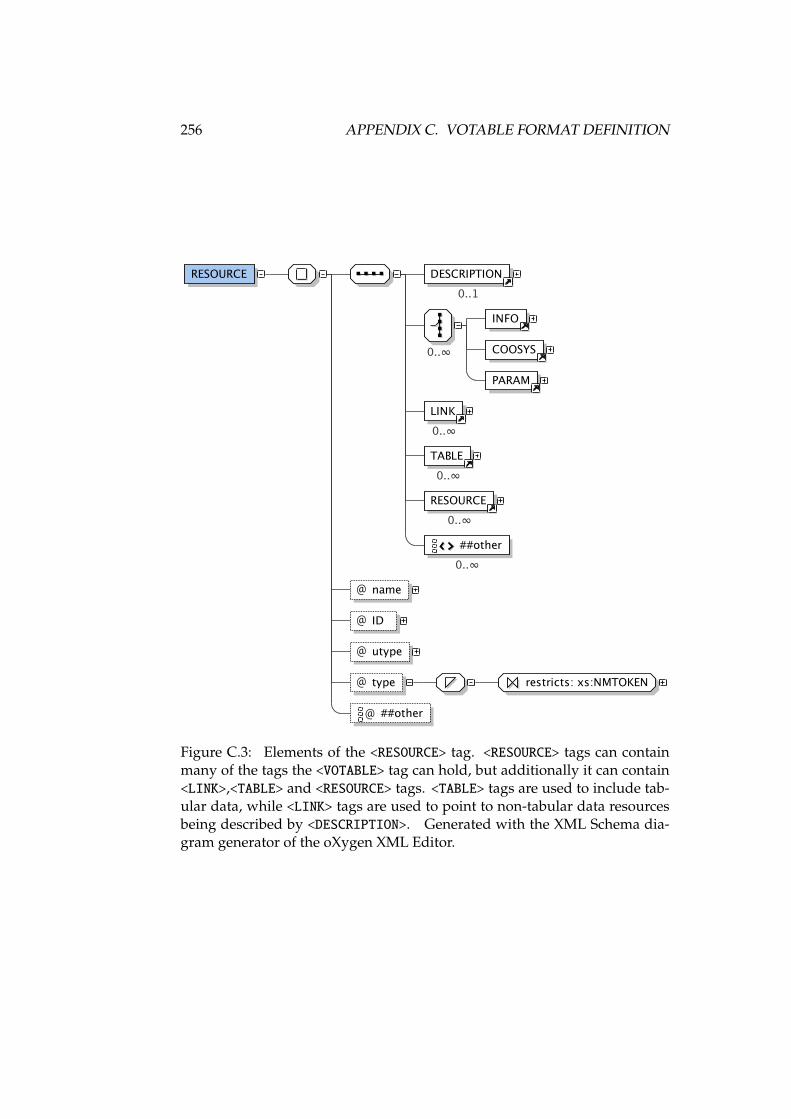
256 APPENDIX C. VOTABLE FORMAT DEFINITION
RESOURCE DESCRIPTION
0..1
0..
INFO
COOSYS
PARAM
LINK
0..
TABLE
0..
RESOURCE
0..
##other
0..
@ name
@ ID
@ utype
@ type restricts: xs:NMTOKEN
@ ##other
Figure C.3: Elements of the <RESOURCE> tag. <RESOURCE> tags can containmany of the tags the <VOTABLE> tag can hold, but additionally it can contain<LINK>,<TABLE> and <RESOURCE> tags. <TABLE> tags are used to include tab-ular data, while <LINK> tags are used to point to non-tabular data resourcesbeing described by <DESCRIPTION>. Generated with the XML Schema dia-gram generator of the oXygen XML Editor.
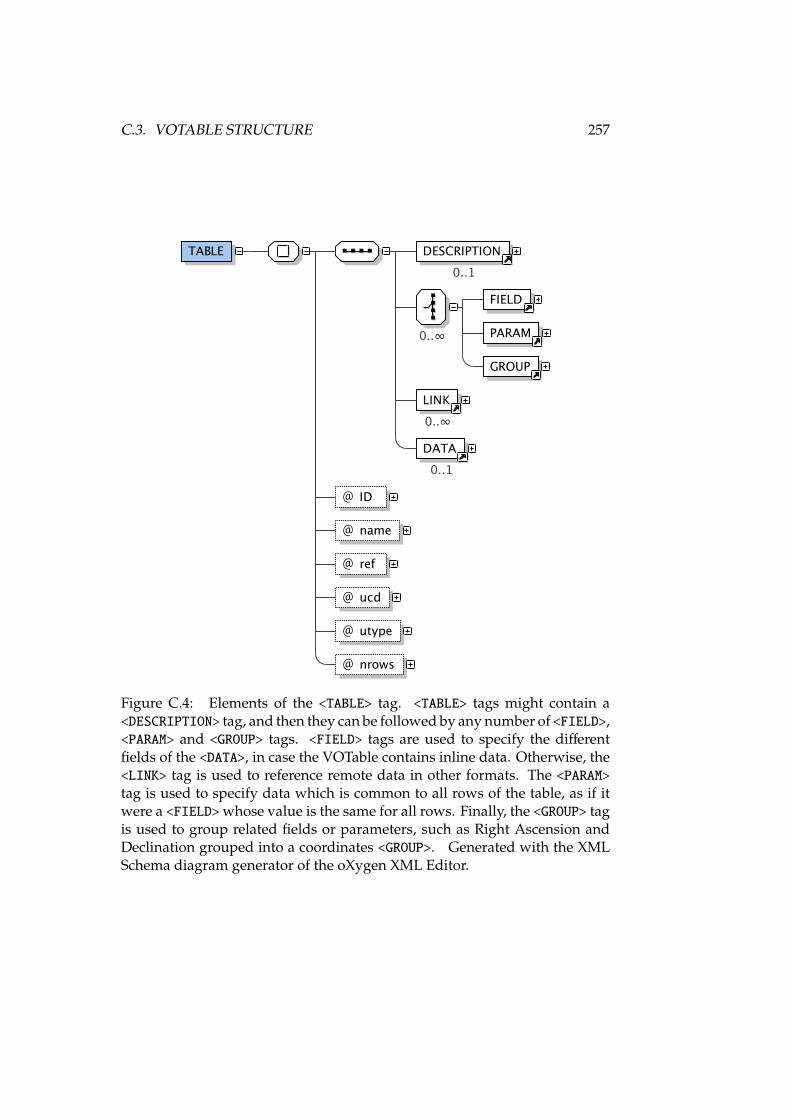
C.3. VOTABLE STRUCTURE 257
TABLE DESCRIPTION
0..1
0..
FIELD
PARAM
GROUP
LINK
0..
DATA
0..1
@ ID
@ name
@ ref
@ ucd
@ utype
@ nrows
Figure C.4: Elements of the <TABLE> tag. <TABLE> tags might contain a<DESCRIPTION> tag, and then they can be followed by any number of <FIELD>,<PARAM> and <GROUP> tags. <FIELD> tags are used to specify the differentfields of the <DATA>, in case the VOTable contains inline data. Otherwise, the<LINK> tag is used to reference remote data in other formats. The <PARAM>tag is used to specify data which is common to all rows of the table, as if itwere a <FIELD> whose value is the same for all rows. Finally, the <GROUP> tagis used to group related fields or parameters, such as Right Ascension andDeclination grouped into a coordinates <GROUP>. Generated with the XMLSchema diagram generator of the oXygen XML Editor.
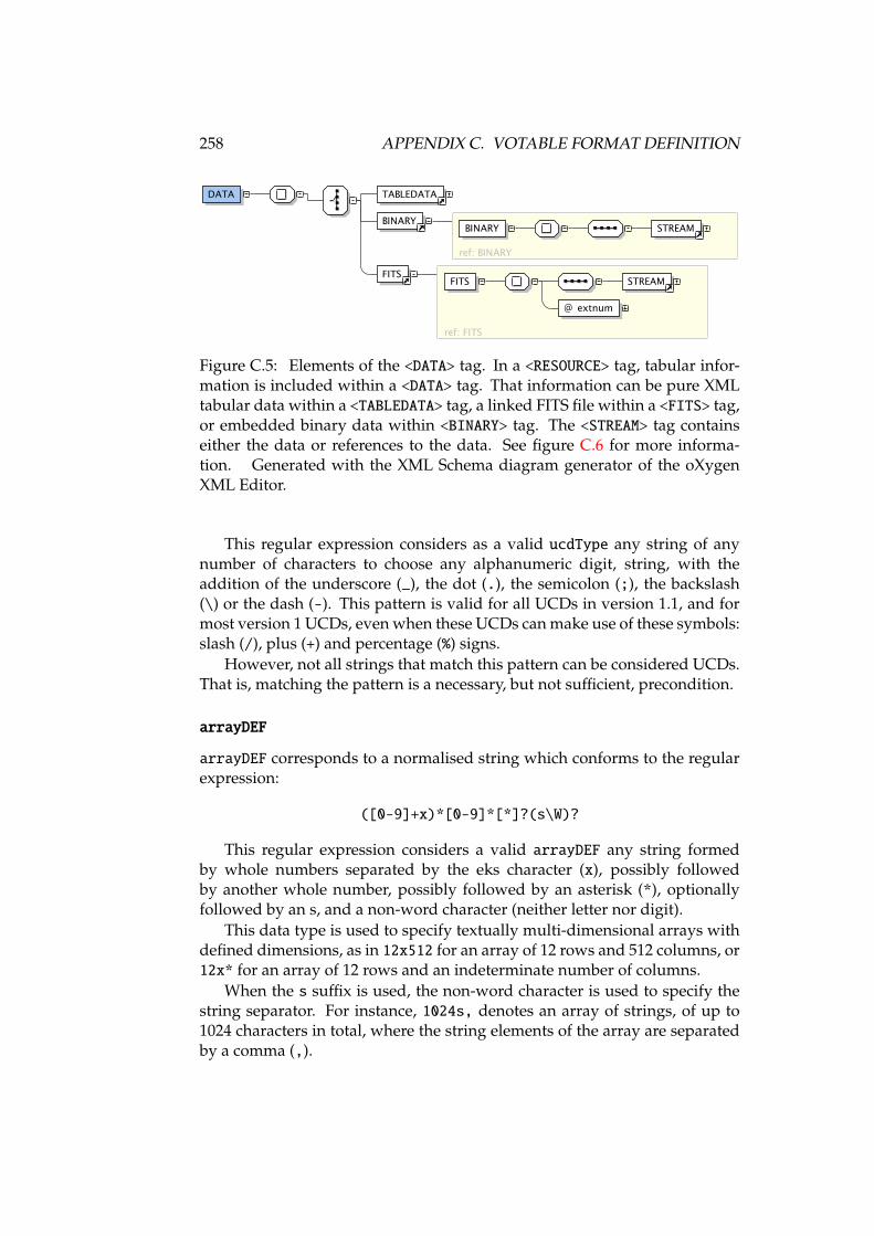
258 APPENDIX C. VOTABLE FORMAT DEFINITION
DATA TABLEDATA
BINARY
ref: BINARY
BINARY STREAM
FITS
ref: FITS
FITS STREAM
@ extnum
Figure C.5: Elements of the <DATA> tag. In a <RESOURCE> tag, tabular infor-mation is included within a <DATA> tag. That information can be pure XMLtabular data within a <TABLEDATA> tag, a linked FITS file within a <FITS> tag,or embedded binary data within <BINARY> tag. The <STREAM> tag containseither the data or references to the data. See figure C.6 for more informa-tion. Generated with the XML Schema diagram generator of the oXygenXML Editor.
This regular expression considers as a valid ucdType any string of anynumber of characters to choose any alphanumeric digit, string, with theaddition of the underscore (_), the dot (.), the semicolon (;), the backslash(\) or the dash (-). This pattern is valid for all UCDs in version 1.1, and formost version 1 UCDs, even when these UCDs can make use of these symbols:slash (/), plus (+) and percentage (%) signs.
However, not all strings that match this pattern can be considered UCDs.That is, matching the pattern is a necessary, but not sufficient, precondition.
arrayDEF
arrayDEF corresponds to a normalised string which conforms to the regularexpression:
([0-9]+x)*[0-9]*[*]?(s\W)?
This regular expression considers a valid arrayDEF any string formedby whole numbers separated by the eks character (x), possibly followedby another whole number, possibly followed by an asterisk (*), optionallyfollowed by an s, and a non-word character (neither letter nor digit).
This data type is used to specify textually multi-dimensional arrays withdefined dimensions, as in 12x512 for an array of 12 rows and 512 columns, or12x* for an array of 12 rows and an indeterminate number of columns.
When the s suffix is used, the non-word character is used to specify thestring separator. For instance, 1024s, denotes an array of strings, of up to1024 characters in total, where the string elements of the array are separatedby a comma (,).

C.3. VOTABLE STRUCTURE 259
STREAM extends: xs:string @ type restricts: xs:NMTOKEN locator
other
base: NMTOKEN from: XMLSchema.xsd
NMTOKEN restricts: xs:token
@ href
@ actuate restricts: xs:NMTOKEN onLoad
onRequest
other
none
base: NMTOKEN from: XMLSchema.xsd
NMTOKEN restricts: xs:token
@ encoding
type: encodingType
encodingType restricts: xs:NMTOKEN gzip
base64
dynamic
none
base: NMTOKEN from: XMLSchema.xsd
NMTOKEN restricts: xs:token
@ expires
type: dateTime from: XMLSchema.xsd
dateTime
@ rights
type: token from: XMLSchema.xsd
token restricts: xs:normalizedString
base: string from: XMLSchema.xsd
string
Figure C.6: Elements of the <STREAM> tag. In this figure we have expanded thedifferent attributes for the <STREAM> tag in order to better understand what hasto be provided. The<STREAM> tag is a string which can contain data encoded inthe formats specified by the encoding attribute, only if the type attribute is notlocator. If the type attribute were locator, the href attribute would containan URI pointing to the actual data source. In any case, an expires attributeexists for transient datasets (for instance, on-demand synthetic datasets, im-age mosaics, or similar non-persistent datasets), the actuate attribute existsfor TODO: Find out what is the actuate attribute used for , and the rightsattribute can be used to store a string (or an escaped XML fragment) whichspecifies in a human readable form the access rights for such data. Generatedwith the XML Schema diagram generator of the oXygen XML Editor.
TABLEDATA TR0..
ref: TR
TR TD1..
Figure C.7: Elements of the <TABLEDATA> tag. Inside the <TABLEDATA> tagseveral <TR> tags can exist, corresponding to different table rows. For eachtable row, there must be as many <TD> tags as <FIELD> tags in the <TABLE>tag containing a particular <TABLEDATA>.
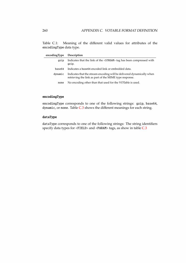
260 APPENDIX C. VOTABLE FORMAT DEFINITION
Table C.1: Meaning of the different valid values for attributes of theencodingType data type.
encodingType Description
gzip Indicates that the link of the <STREAM> tag has been compressed withgzip.
base64 Indicates a base64 encoded link or embedded data.
dynamic Indicates that the stream encoding will be delivered dynamically whenretrieving the link as part of the MIME type response.
none No encoding other than that used for the VOTable is used.
encodingType
encodingType corresponds to one of the following strings: gzip, base64,dynamic, or none. Table C.3 shows the different meanings for each string.
dataType
dataType corresponds to one of the following strings: The string identifiersspecify data types for <FIELD> and <PARAM> tags, as show in table C.3
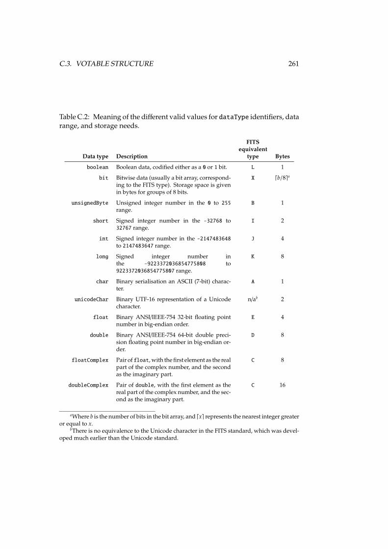
C.3. VOTABLE STRUCTURE 261
Table C.2: Meaning of the different valid values for dataType identifiers, datarange, and storage needs.
FITSequivalent
Data type Description type Bytes
boolean Boolean data, codified either as a 0 or 1 bit. L 1
bit Bitwise data (usually a bit array, correspond-ing to the FITS type). Storage space is givenin bytes for groups of 8 bits.
X db/8ea
unsignedByte Unsigned integer number in the 0 to 255range.
B 1
short Signed integer number in the -32768 to32767 range.
I 2
int Signed integer number in the -2147483648to 2147483647 range.
J 4
long Signed integer number inthe -9223372036854775808 to9223372036854775807 range.
K 8
char Binary serialisation an ASCII (7-bit) charac-ter.
A 1
unicodeChar Binary UTF-16 representation of a Unicodecharacter.
n/ab 2
float Binary ANSI/IEEE-754 32-bit floating pointnumber in big-endian order.
E 4
double Binary ANSI/IEEE-754 64-bit double preci-sion floating point number in big-endian or-der.
D 8
floatComplex Pair offloat, with the first element as the realpart of the complex number, and the secondas the imaginary part.
C 8
doubleComplex Pair of double, with the first element as thereal part of the complex number, and the sec-ond as the imaginary part.
C 16
aWhere b is the number of bits in the bit array, and dxe represents the nearest integer greateror equal to x.
bThere is no equivalence to the Unicode character in the FITS standard, which was devel-oped much earlier than the Unicode standard.

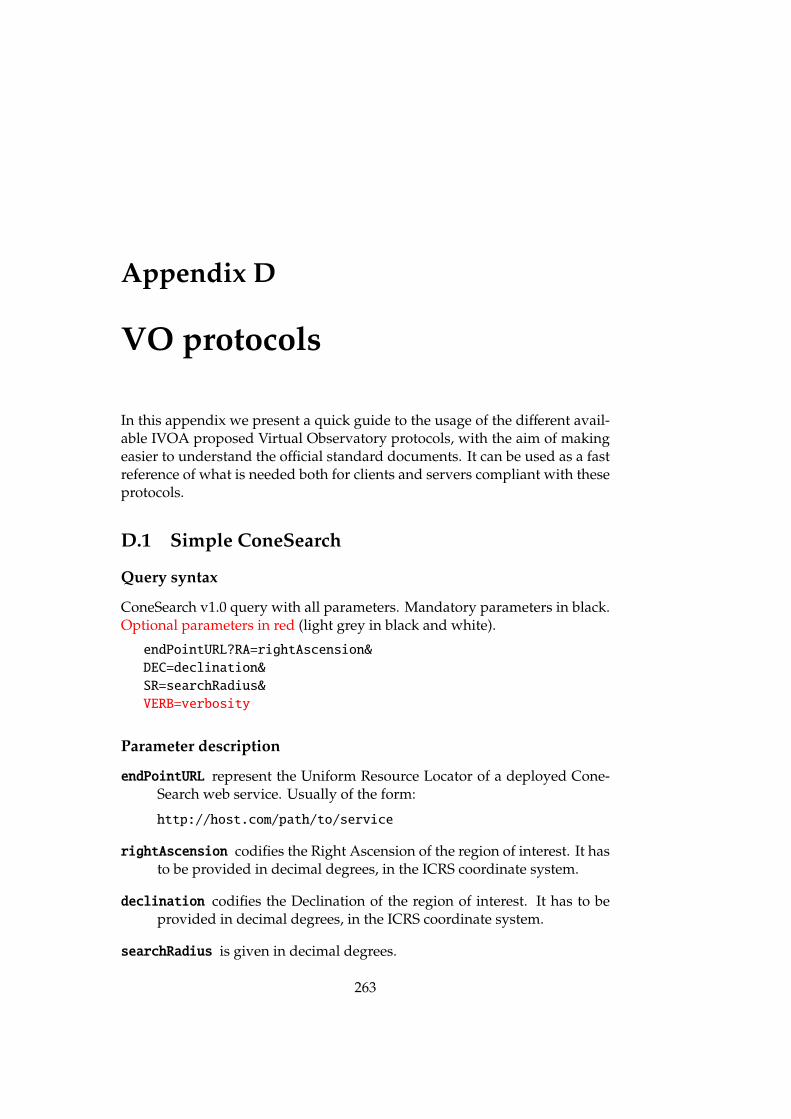
Appendix D
VO protocols
In this appendix we present a quick guide to the usage of the different avail-able IVOA proposed Virtual Observatory protocols, with the aim of makingeasier to understand the official standard documents. It can be used as a fastreference of what is needed both for clients and servers compliant with theseprotocols.
D.1 Simple ConeSearch
Query syntax
ConeSearch v1.0 query with all parameters. Mandatory parameters in black.Optional parameters in red (light grey in black and white).
endPointURL?RA=rightAscension&DEC=declination&SR=searchRadius&VERB=verbosity
Parameter description
endPointURL represent the Uniform Resource Locator of a deployed Cone-Search web service. Usually of the form:
http://host.com/path/to/service
rightAscension codifies the Right Ascension of the region of interest. It hasto be provided in decimal degrees, in the ICRS coordinate system.
declination codifies the Declination of the region of interest. It has to beprovided in decimal degrees, in the ICRS coordinate system.
searchRadius is given in decimal degrees.
263
264 APPENDIX D. VO PROTOCOLS
verbosity specifies reply verbosity; verbosity can be one of 1, 2 or 3. 1provides the least verbose reply, and 3 the most verbose.
Service reply
A ConeSearch service reply consist of a VOTABLE, with complies with thefollowing :
• The VOTABLE response contains just one RESOURCE, which containsjust one TABLE.
• Table fields:
– Exactly ONE field has UCD="ID_MAIN", with the string data type,which provides an unique ID for each table row/record.
– Exactly ONE field has UCD="POS_EQ_RA_MAIN", with data typedouble, representing the Right Ascension of the observed sourcein the ICRS coordinate system.
– Exactly ONE field has UCD="POS_EQ_DEC_MAIN", with data typedouble, representing the Declination of the observed source in theICRS coordinate system.
– An additional <FIELD> or <PARAM> tag with UCD="OBS_ANG-SIZE"can be used to specify a per-record (<FIELD>) or per-table (<PARAM>)positional error on source positions, or angular size for resolvedobservations.
– The rest of the returned fields depend on the catalog,but all<FIELD>or <PARAM> tags should specify description, data type, and UCD.
D.2 Simple Image Access Protocol
Query syntax
Mandatory query parameters listed in black. Optional parameters listedin blue. Not all services implement all optional parameters, except forFORMAT=formatType. Use metadata as formatType to retrieve supportedparameters.
endPointURL?POS=RA,DEC&SIZE=searchRadius&FORMAT=formatType&INTERSECT=intersectionMechanism&NAXIS=axisSizeVector&CFRAME=coordFrame&EQUINOX=equinoxSpec&
D.2. SIMPLE IMAGE ACCESS PROTOCOL 265
CRPIX=refPixCoordVector&CRVAL=refPixValueVector&CDELT=pixScaleVector&ROTANG=rotationAngle&PROJ=projectionKind&VERB=verbosity
Parameter description
endPointURL represents the Uniform Resource Locator of a deployed SIAPweb service. Usually of the form:
http://host.com/path/to/service
RA,DEC is a pair of double quantities, separated by a comma (,), represent-ing Right Ascension and Declination in decimal degrees. No officialconsideration of coordinate system, but ICRS can be assumed.
searchRadius is either a double quantity, or a pair of double quantitiesseparated by a comma (,). If a pair of values is specified, the first isassumed to be an RA width, and the second a DEC width. The regionthus defined has constant RA and DEC edges. The combination of POSand SIZE will be called region of interest (ROI) in the following.
formatType is a string representation of the MIME media type of files beingasked for to the service. It will be one of:
• image/fits
• image/png
• image/jpeg
• text/html
• fits (equivalent to image/fits)
• graphic (equivalent to image/png; image/jpeg)
• all (default value)
Additionally, if formatType is metadata, the service will reply with aVOTABLE with all supported input parameters.
intersectionMechanism specifies how to evaluate the intersection of candi-date images with the ROI specified. It has to be ONE of the following:
COVERS: returned images completely includes (covers) the entire ROI.
ENCLOSED: returned images are completely covered (enclosed) by theROI. Uses the same mechanism of COVERS, reversing the role ofROI and test image.
266 APPENDIX D. VO PROTOCOLS
CENTER: returned images include at least the center of the ROI. This isan special case of OVERLAPS.
OVERLAPS: returned images have some common points with the spec-ified ROI. OVERLAPS should return at least all images returned byCENTER.
axisSizeVector is the size of the output image in pixels. This is a vector-valued quantity, expressed as NAXIS=<width>,<height>.
coordFrame is a string specifying a coordinate system reference frame. It isone of:
• ICRS (default)
• FK5
• FK4
• ECL
• GAL
• SGAL
equinoxSpec is the epoch of the mean equator and equinox for the coordinatesystem reference frame specified by coordFrame. It is not required forICRS, and defaults to B1950 for FK4, and to J2000 otherwise.
refPixCoordVector provides the coordinates of the reference pixel, in pixelcoordinates of the output image. This is a vector-valued quantity of thesame size as axisSizeVector.
refPixValueVector is a vector of the world coordinates relative tocoordFrameat the refPixCoordVector. Defaults to the ROI center coordinates,transformed to the output coordinate system reference if other thanICRS.
pixScaleVector provides the scale of the output image in decimal degreesper pixel. A negative value implies an axis flip. Since the default imageorientation is N up and E to the left, the default sign of pixScaleVectoris [-1,1]. Can be given as comma separated vector, or as a single value;if only one value is given, it applies to both image axes.
rotationAngle specifies the rotation angle for the output image in degreesrelative to coordFrame (an image which is unrotated in one referenceframe may be rotated in another). Rotation of the WCS declination orlatitude axis with respect to the second axis of the image, measured inthe counterclockwise direction (following FITS WCS convention, whichin turn is based on the old AIPS convention). Defaults to 0 (no rotation).
D.2. SIMPLE IMAGE ACCESS PROTOCOL 267
projectionKind specifies the celestial projection of the output image; is oneof TAN, SIN, ARC, et cetera. Defaults to TAN.
verbosity is an integer value, ranging from 0 to 3 that specifies replyverbosity (how much additional meta data are provided).
Optional parameters: query with all mandatory and optional parameters inversion 1:
Remember that parameters not supported by the service will be dis-carded. Call the service with FORMAT=metadata to retrieve supportedparameters (see below).
SIAP v2 extensions: query with mandatory and extended parameters:
endPointURL?POS=RA,DEC&SIZE=searchRadius&REQUEST=requestKind&TIME=timeSpec&ANGRP=angularResolution&PUBDID=pubID&CREATORDID=creatorID&COLLECTION=collectionID&TOP=topNumResults&MAXREC=maxRecords&MTIME=incorporationTime&COMPRESS=compressionFlag&RUNID=jobRunID&REDSHIFT=redShiftRange&TARGETNAME=targetName
See SSAP for explanations on TIME, PUBDID, CREATORDID, COLLECTION,TOP, MAXREC, MTIME, COMPRESS, RUNID, REDSHIFT and TARGETNAME.
requestKind specifies the kind of image services being required: cut-out, mosaicing, atlas archive, pointed archive. A service can sup-port all or some (at least one) of these request kinds.
angularResolution specifies the angular resolving power of the im-age, for interpolated images.
SIAP multidimensional extensions: for SIAP to be extended to support mul-tidimensional data sets, keywordsNAXIS,CRPIX,CRVALandCDELT shouldbe enhanced to specify N dimensions (typically, N ∈ 3, 4); first twoshould always be RA and DEC, with either time, frequency wavelengthor velocity as the third dimension, and polarisation as a fourth axis, ifpresent.
268 APPENDIX D. VO PROTOCOLS
D.3 Simple Spectral Access Protocol
Query syntax
Parameters all SSAP compliant services need to implement are in black. Pa-rameters whose implementation is optional, but recommended, appear inblue, and parameters whose implementation is completely optional appearin red.
endPointURL?POS=RA,DEC&SIZE=searchRadius&BAND=freqRange&TIME=timeRange&FORMAT=formatType&SPECRP=specResol&SPATRES=spatialResol&PUBDID=pubID&CREATORDID=creatorID&COLLECTION=collectionID&TOP=topNumResults&MAXREC=maxRecords&MTIME=modificationTime&COMPRESS=compressionFlag&RUNID=jobRunID&APERTURE=apertAngle&TIMERES=timeResol&SNR=signal2noise&REDSHIFT=redShiftRange&VARAMPL=amplitudeVariability&TARGETNAME=targetName&TARGETCLASS=targetClass&FLUXCALIB=fluxCalibKind&WAVECALIB=waveCalibKind
None of the service mandatory parameters is needed per se in a particularquery: the following are legal, minimal SSAP queries:
endPointURL?POS=RA,DEC&SIZE=searchRadius
endPointURL?TIME=timeRange&BAND=freqRange
Parameter description
The following is a description of the different SSAP parameters. In SSAP,parameters can be qualified by juxtaposing additional qualifiers, separatedby a semicolon (;). Appropriate qualifiers will be pointed out as needed.
D.3. SIMPLE SPECTRAL ACCESS PROTOCOL 269
endPointURL represents the Uniform Resource Locator of a deployed SIAPweb service. Usually of the form:
http://host.com/path/to/service
RA,DEC is a pair of double quantities, separated by a comma (,), represent-ing Right Ascension and Declination in decimal degrees, in the ICRScoordinate system unless otherwise specified.
POS=RA,DEC can be substituted by GALACTICPOS=GalLat,GalLong. Notall services need to support GALACTICPOS.
searchRadius is either a double quantity, or a pair of double quantitiesseparated by a comma (,). If a pair of values is specified, the first isassumed to be an RA width, and the second a DEC width. The regionthus defined has constant RA and DEC edges. The combination of POSand SIZE will be called region of interest (ROI) in the following.
freqRange specifies a frequency range the query should be restricted to,expressed as low/high wavelengths in meters: BAND=2.7E-7/0.13. Asource qualifier can be used to specify that the frequencies are beingspecified at the source LSR: BAND=0.001/0.01;source
timeRange restricts the query to a given date, specified as an ISO 8601 [1]date-time string (e.g., TIME=1998-05-21), or a date-time range in UTC:TIME=1998-05-21/1999). Qualifiers can be used to specify Local Side-real Time or other time zones:
TIME=2003-04-01T02:00:00/2003-04-01T06:00:00;LST.
formatType is a string representation of the MIME media type of files beingasked for to the service. It will be one of:
• application/fits
• compliant (votable or xml)
• native (native format of the archive)
• graphic (PNG, JPEG or EPS)
• votable (compare with XML)
• fits (equivalent to application/fits)
• xml (SED XML serialisation)
• all (default value)
270 APPENDIX D. VO PROTOCOLS
Additionally, if formatType is metadata, the service will reply with aVOTABLE with all supported input parameters.
formatType can be qualified by the conventions used for spectral re-duction, such as convention=STScI-STIS.
specResol is a double specifying spectral resolving power, λ∆λ ; specResol is
a dimensionless quantity.
spatialResol is a double specifying the minimum spatial resolution, indecimal degrees, corresponding to signal PSF.
pubID is a string holding the NASA ADS publication ID.
creatorID is a string specifying the IVORN for the data set creator.
collectionID is a string specifying an IVORN for a particular collection, ora short-name: for instance, the short-name HST Spectra, or its IVORN:ivo://mast.stsci/ssap/hst.
topNumResults is an integer specifying the maximum number of results tobe returned by the query, but requesting them sorted by an heuristicscore defined by the service. That score is built to be higher for bettermatching records. In any case, the same query should always returnthe same topNumResults records. Default value is up to the service, butshould be small enough to deliver fast responses.
maxRecords is an integer specifying the maximum number of results to bereturned by the query. The same query might return different recordsdepending on service implementation. Default value is up to the ser-vice, but should be small enough to deliver fast responses.
modificationTime is similar to timeRange in syntax, but refers to recordcreation or modification date-time.
compressionFlag is astring containing eithertrueorfalse. IfcompressionFlagis true, returned data might be compressed. Default is false.
jobRunID is a string with contains a client side request ID, so that recordsfrom different services, called with the same jobRunID, can be easilyaggregated.
apertAngle is a double used to specify a synthetic aperture angle in decimaldegrees in order to extract spectra from data cubes, event lists or otherfundamental data. For extraction services, this parameter is mandatory,and the service should provide a sensible default.
timeResol is a double specifying minimum time resolution in seconds (typ-ically, the bounds of the exposure time coverage).
D.3. SIMPLE SPECTRAL ACCESS PROTOCOL 271
signal2noise is a dimensionless double specifying the Signal to Noise ratio,as a number of times noise RMS.
redShiftRange is a string encoding a double or a range of doubles, whichspecifies a particular dimensionless redshift or range, calculated us-ing the optical convention z = ∆λ
λ : REDSHIFT=1.3/3.0 means z ∈[1.3, 3.0], REDSHIFT=1.3/ means z ∈ [1.3,+∞), while querying withREDSHIFT=/3.0 means z ∈ [0, 3.0]. Negative values can be used toindicate blueshifts.
amplitudeVariability is dimensionless double in the range [0.0,1.0] indi-cating amplitude variations from the maximum.
targetName is a string providing the name of target that will need to beresolved by SIMBAD, NED, o similar services. To be used instead ofcoordinates.
targetClass is a string providing comma delimited list of types of astro-nomical objects to be searched for. Valid types form controlled vocabu-lary coming from Simbad [3]. Eventually types should come from theIVOA Thesaurus.
fluxCalibKind is a string encoding a boolean value (true or false) indi-cating whether we require returned data fluxes to be calibrated. Nodistinction is made between absolute or relative flux calibration.
waveCalibKind is a string encoding a boolean value (true or false) indicat-ing whether we require returned data wavelengths to be calibrated. Nodistinction is made between absolute or relative wavelength calibration.

Bibliografía
[1] A. Comte, The positive philosophy of Auguste Comte, vol. 1 of 2, ch. I: GeneralView of Book II: Astronomy. London: G. Bell and sons, 1896. 1.1
[2] G. de Vaucouleurs, Astronomical photography. From the daguerrotype to theelectron camera. London: Faber & Faber, 1961, 1961. 1.1
[3] P. Abrahams, “The early history of astrophotography.” 1.1
[4] K. G. Jansky, “Electrical disturbances apparently of extraterrestrial ori-gin,” Proceedings of the Institute of Radio Engineers, vol. 21, pp. 1387–1398,October 1933. 1.1
[5] K. G. Jansky, “A note on the source of interstellar interference,” Procee-dings of the Institute of Radio Engineers, vol. 23, pp. 1158–1163, October1935. 1.1
[6] R. W. Wilson, “The cosmic microwave background radiation,” Science,vol. 205, pp. 866–874, Aug. 1979. 1.1
[7] A. A. Penzias, “The origin of the elements,” Science, vol. 205, pp. 549–554,Aug. 1979. 1.1
[8] S. V. W. Beckwith, M. Stiavelli, A. M. Koekemoer, J. A. R. Caldwell, H. C.Ferguson, R. Hook, R. A. Lucas, L. E. Bergeron, M. Corbin, S. Jogee,N. Panagia, M. Robberto, P. Royle, R. S. Somerville, and M. Sosey, “TheHubble Ultra Deep Field,” The Astronomical Journal, vol. 132, pp. 1729–1755, Nov. 2006. 1.1
[9] D. C. Wells, E. W. Greisen, and R. H. Harten, “FITS: A Flexible ImageTransport System,” Astronomy & Astrophysics, Supplement Series, vol. 44,pp. 363–+, June 1981. 1.2, 2.3, B.1
[10] J. Gunn and D. Weinberg, “The Sloan Digital Sky Survey,” in WideField Spectroscopy and the Distant Universe (S. J. Maddox and A. Aragon-Salamanca, eds.), pp. 3–+, 1995. 1.2
273
274 BIBLIOGRAFÍA
[11] D. G. York, J. Adelman, J. E. Anderson, Jr., S. F. Anderson, J. Annis,N. A. Bahcall, J. A. Bakken, R. Barkhouser, S. Bastian, E. Berman, W. N.Boroski, S. Bracker, C. Briegel, J. W. Briggs, J. Brinkmann, R. Brunner,S. Burles, L. Carey, M. A. Carr, F. J. Castander, B. Chen, P. L. Colestock,A. J. Connolly, J. H. Crocker, I. Csabai, P. C. Czarapata, J. E. Davis, M. Doi,T. Dombeck, D. Eisenstein, N. Ellman, B. R. Elms, M. L. Evans, X. Fan,G. R. Federwitz, L. Fiscelli, S. Friedman, J. A. Frieman, M. Fukugita,B. Gillespie, J. E. Gunn, V. K. Gurbani, E. de Haas, M. Haldeman, F. H.Harris, J. Hayes, T. M. Heckman, G. S. Hennessy, R. B. Hindsley, S. Holm,D. J. Holmgren, C.-h. Huang, C. Hull, D. Husby, S.-I. Ichikawa, T. Ichika-wa, Z. Iveziç, S. Kent, R. S. J. Kim, E. Kinney, M. Klaene, A. N. Kleinman,S. Kleinman, G. R. Knapp, J. Korienek, R. G. Kron, P. Z. Kunszt, D. Q.Lamb, B. Lee, R. F. Leger, S. Limmongkol, C. Lindenmeyer, D. C. Long,C. Loomis, J. Loveday, R. Lucinio, R. H. Lupton, B. MacKinnon, E. J. Man-nery, P. M. Mantsch, B. Margon, P. McGehee, T. A. McKay, A. Meiksin,A. Merelli, D. G. Monet, J. A. Munn, V. K. Narayanan, T. Nash, E. Neil-sen, R. Neswold, H. J. Newberg, R. C. Nichol, T. Nicinski, M. Nonino,N. Okada, S. Okamura, J. P. Ostriker, R. Owen, A. G. Pauls, J. Peoples,R. L. Peterson, D. Petravick, J. R. Pier, A. Pope, R. Pordes, A. Prosapio,R. Rechenmacher, T. R. Quinn, G. T. Richards, M. W. Richmond, C. H.Rivetta, C. M. Rockosi, K. Ruthmansdorfer, D. Sandford, D. J. Schlegel,D. P. Schneider, M. Sekiguchi, G. Sergey, K. Shimasaku, W. A. Siegmund,S. Smee, J. A. Smith, S. Snedden, R. Stone, C. Stoughton, M. A. Strauss,C. Stubbs, M. SubbaRao, A. S. Szalay, I. Szapudi, G. P. Szokoly, A. R.Thakar, C. Tremonti, D. L. Tucker, A. Uomoto, D. Vanden Berk, M. S.Vogeley, P. Waddell, S.-i. Wang, M. Watanabe, D. H. Weinberg, B. Yanny,and N. Yasuda, “The Sloan Digital Sky Survey: Technical Summary,” TheAstronomical Journal, vol. 120, pp. 1579–1587, Sept. 2000. 1.2
[12] M. F. Skrutskie, R. M. Cutri, R. Stiening, M. D. Weinberg, S. Schneider,J. M. Carpenter, C. Beichman, R. Capps, T. Chester, J. Elias, J. Huchra,J. Liebert, C. Lonsdale, D. G. Monet, S. Price, P. Seitzer, T. Jarrett, J. D.Kirkpatrick, J. E. Gizis, E. Howard, T. Evans, J. Fowler, L. Fullmer, R. Hurt,R. Light, E. L. Kopan, K. A. Marsh, H. L. McCallon, R. Tam, S. VanDyk, and S. Wheelock, “The Two Micron All Sky Survey (2MASS),” TheAstronomical Journal, vol. 131, pp. 1163–1183, Feb. 2006. 1.2
[13] R. H. Becker, R. L. White, and D. J. Helfand, “The VLA’s FIRST Survey,”in Astronomical Data Analysis Software and Systems III (D. R. Crabtree, R. J.Hanisch, and J. Barnes, eds.), vol. 61 of Astronomical Society of the PacificConference Series, pp. 165–+, 1994. 1.2
[14] J. J. Condon, W. D. Cotton, E. W. Greisen, R. A. Perley, Q. F. Yin, andJ. J. Broderick, “The NRAO VLA Sky Survey,” in Bulletin of the American
275
Astronomical Society, vol. 25 of Bulletin of the American Astronomical Society,pp. 1389–+, Dec. 1993. 1.2
[15] M. P. Haynes and the ALFALFA Team, “The Arecibo Legacy Fast ALFA(ALFALFA) Extragalactic HI Survey,” ArXiv e-prints, vol. 806, June 2008.1.2
[16] R. Giovanelli, M. P. Haynes, B. R. Kent, P. Perillat, A. Saintonge,N. Brosch, B. Catinella, G. L. Hoffman, S. Stierwalt, K. Spekkens, M. S.Lerner, K. L. Masters, E. Momjian, J. L. Rosenberg, C. M. Springob, A. Bo-selli, V. Charmandaris, J. K. Darling, J. Davies, D. G. Lambas, G. Gavazzi,C. Giovanardi, E. Hardy, L. K. Hunt, A. Iovino, I. D. Karachentsev, V. E.Karachentseva, R. A. Koopmann, C. Marinoni, R. Minchin, E. Muller,M. Putman, C. Pantoja, J. J. Salzer, M. Scodeggio, E. Skillman, J. M. So-lanes, C. Valotto, W. van Driel, and L. van Zee, “The Arecibo LegacyFast ALFA Survey. I. Science Goals, Survey Design, and Strategy,” TheAstronomical Journal, vol. 130, pp. 2598–2612, Dec. 2005. 1.2
[17] G. E. Moore, “Cramming more components onto integrated circuits,”Electronics, vol. 38, April 1965. 1.3
[18] European Southern Observatory (ESO), “The ESO/ST-ECF Science Ar-chive Facility: An overview of our services,” brochure, European Sout-hern Observatory, Space Telescope European Coordination Facility, April2004. 1.2
[19] A. S. Szalay and J. Gray, “The World-Wide Telescope,” Science, vol. 293,pp. 2037–2040, Sept. 2001. 1.3, 2.1, 2.2
[20] F. Genova, “Interoperability,” in Astronomical Data Analysis Software andSystems XI (D. A. Bohlender, D. Durand, and T. H. Handley, eds.), vol. 281of Astronomical Society of the Pacific Conference Series, pp. 41–+, 2002. 2.1
[21] C. Flatters, “The FITS Interferometry Data Interchange Format,” AIPSMemo 102, National Radio Astronomy Observatory, Associated Univer-sities, Inc., Washington DC, USA, August 2000. 2.3
[22] D. Muders, E. Polehampton, and J. Hatchell, “Multi-Beam FITS RawData Format,” tech. rep., Max-Planck-Instituts für Radioastronomie, De-cember 2005. 2.3, 6, 6.1
[23] R. W. Garwood, “SDFITS: A Standard for Storage and Interchange ofSingle Dish Data,” in Astronomical Data Analysis Software and Systems IX(N. Manset, C. Veillet, and D. Crabtree, eds.), vol. 216 of AstronomicalSociety of the Pacific Conference Series, pp. 243–+, 2000. 2.3
276 BIBLIOGRAFÍA
[24] FITS Working Group, “Definition of the Flexible Image TransportSystem (FITS),” FITS Standard Version 3.0, Commission 5: Docu-mentation and Astronomical Data-International Astronomical Union,http://fits.gsfc.nasa.gov/iaufwg/, July 2008. 2.3
[25] F. Ochsenbein, M. Albrecht, A. Brighton, P. Fernique, D. Guillaume, R. J.Hanisch, E. Shaya, and A. Wicenec, “Using XML for Accessing Resourcesin Astronomy,” in Astronomical Data Analysis Software and Systems IX(N. Manset, C. Veillet, and D. Crabtree, eds.), vol. 216 of AstronomicalSociety of the Pacific Conference Series, pp. 83–+, 2000. 2.3, A.1
[26] B. Thomas, E. Shaya, and C. Cheung, “Converting FITS into XML: Met-hods and Advantages,” in Astronomical Data Analysis Software and SystemsX (F. R. Harnden, Jr., F. A. Primini, and H. E. Payne, eds.), vol. 238 ofAstronomical Society of the Pacific Conference Series, pp. 487–+, 2001. 2.3
[27] K. Blackburn, A. Lazzarini, T. Prince, and R. Williams, XSIL: Extensiblescientific interchange language, vol. 1593/1999 of Lecture Notes in ComputerScience, pp. 513–524. Springer, 1999. 2.3
[28] E. Shaya, B. Thomas, J. Gass, J. Blackwell, and C. Cheung, “XDF - anXML-based Scientific Interchange Language,” in Bulletin of the AmericanAstronomical Society, vol. 32 of Bulletin of the American Astronomical Society,pp. 1600–+, Dec. 2000. 2.3
[29] D. Tody and R. Plante, “Simple Image Access Protocol,” IVOA WorkingDraft 1.01, International Virtual Observatory Alliance, October 2008. 2.4
[30] D. Tody and M. Dolensky, “Simple Spectral Access Protocol,” IVOAProposed Recommendation Version 1.01, International Virtual Ob-servatory Alliance, file://localhost/Users/jdsant/Documents/IAA/SSA-20070604.pdf 2007. 2.4, A.1
[31] M. Dolensky and D. Tody, “The Simple Spectral Access protocol,” inSociety of Photo-Optical Instrumentation Engineers (SPIE) Conference Series(P. J. Quinn and A. Bridger, eds.), vol. 5493 of Society of Photo-OpticalInstrumentation Engineers (SPIE) Conference Series, pp. 262–268, Sept. 2004.2.4
[32] R. Williams, R. Hanisch, A. Szalay, and R. Plante, “Simple cone search,”Proposed Recommendation Version 1.03, International Virtual Observa-tory Alliance, February 2008. 2.4, A.1
[33] C. Lagoze, H. Van de Sompel, M. Nelson, and S. Warner, “The OpenArchives Initiative Protocol for Metadata Harvesting,” Tech. Rep. v2.0,Open Archives Initiative, June 2002. 2.8
277
[34] J. Kunze, R. Guenther, M. Hlava, C. Morgan, and J. Perkins, “The DublinCore Metadata Element Set,” American National Standard Z39-85-2007,ANSI/NISO, NISO Press, Bethesda, Maryland, U.S.A., May 2007. 2.8
[35] R. Plante, K. Benson, M. Graham, G. Greene, P. Harrison, G. Lemson,T. Linde, G. Rixon, and A. Stébé, “VOResource: an XML Encoding Sche-ma for Resource Metadata,” IVOA Recommendation v1.03, InternationalVirtual Observatory Alliance, February 2008. 2.8
[36] R. Plante, A. Stébé, K. Benson, M. Graham, G. Greene, P. Harrison, T. Lin-de, G. Rixon, and IVOA Registry WG, “VODataService: a VOResourceSchema extension for describing collections and services,” IVOA Wor-king Draft v1.01, International Virtual Observatory Alliance, October2008. 2.8
[37] P. Quinn, R. Hanisch, and A. Lawrence, “IVOA Statement and Roadmap2002-2005,” June 2002. 2.9
[38] D. de Young, G. Djorgovski, F. Genova, K. Gorski, B. Hanisch,A. Kembhavi, A. Lawrence, T. Linde, O. Malkov, R. Moore, R. Norris,P. Quinn, B. Pirenne, D. Schade, A. S. Szalay, V. Vitkovsky, W. Voges,N. A. Walton, and R. Williams, “First IVOA Full Meeting,” MinutesFM1, International Virtual Observatory Alliance, Garching bei Mün-chen, Germany (http://www.ivoa.net/internal/IVOA/IvoaRepMin/ivoa-fm1-20020613.pdf), June 2002. 2.9
[39] P. J. Quinn and K. M. Górski, eds., Toward an International Virtual Obser-vatory, 2004. 2.9
[40] P. J. Quinn, M. Allen, K. Andrews, T. Boch, F. Bonnarel, S. Derriere,M. Dolensky, P. Fernique, M. Hill, M. C. Leoni, A. Linde, A. Micol,B. Pirenne, A. M. S. Richards, A. Schaaff, G. Tissier, N. A. Walton, andA. Wicenec, “The AVO Prototype,” in Astronomical Data Analysis Softwareand Systems (ADASS) XIII (F. Ochsenbein, M. G. Allen, and D. Egret, eds.),vol. 314 of Astronomical Society of the Pacific Conference Series, pp. 304–+,July 2004. 2.9
[41] R. Gutiérrez, C. Rodrigo, and E. Solano, “The Spanish Virtual Obser-vatory (SVO),” in Astronomical Data Analysis Software and Systems XV(C. Gabriel, C. Arviset, D. Ponz, and E. Solano, eds.), vol. 351 of ASPConference Series, pp. 19–+, July 2006. 2.9
[42] P. Harrison, “A proposal for a Common Execution Architecture,” IVOAWG Internal Draft 2005-05-12 Version 1.2, International Virtual Obser-vatory Alliance, May 2005. 2.10, A.1
278 BIBLIOGRAFÍA
[43] B. F. Madore, G. Helou, H. G. Corwin, Jr., M. Schmitz, X. Wu, and J. Ben-nett, “The NASA/IPAC Extragalactic Database,” in Astronomical DataAnalysis Software and Systems I (D. M. Worrall, C. Biemesderfer, andJ. Barnes, eds.), vol. 25 of Astronomical Society of the Pacific ConferenceSeries, pp. 47–+, 1992. 2.11
[44] M. Wenger, F. Ochsenbein, D. Egret, P. Dubois, F. Bonnarel, S. Borde,F. Genova, G. Jasniewicz, S. Laloë, S. Lesteven, and R. Monier, “TheSIMBAD astronomical database. The CDS reference database for astro-nomical objects,” Astronomy & Astrophysics, Supplement Series, vol. 143,pp. 9–22, Apr. 2000. 2.11
[45] F. Ochsenbein, P. Bauer, and J. Marcout, “The VizieR database of astrono-mical catalogues,” Astronomy & Astrophysics, Supplement Series, vol. 143,pp. 23–32, Apr. 2000. 2.11
[46] M. J. Kurtz, G. Eichhorn, A. Accomazzi, C. S. Grant, S. S. Murray, and J. M.Watson, “The NASA Astrophysics Data System: Overview,” Astronomy& Astrophysics, Supplement Series, vol. 143, pp. 41–59, Apr. 2000. 2.11
[47] I. Foster and C. Kesselman, Computational Grids, ch. 2. Morgan-Kaufman,1999. 2.12
[48] A. Chervenak, I. Foster, C. Kesselman, C. Salisbury, and S. Tuecke, “Thedata grid: Towards an architecture for the distributed management andanalysis of large scientific datasets,” Journal of Network and ComputerApplications, vol. 23, pp. 187–200, 2001. 2.12
[49] M. Graham, D. Morris, and G. Rixon, “VOSpace specification,” Propo-sed Recommendation Version 1.14, International Virtual ObservatoryAlliance, October 2008. 2.12
[50] P. Z. Kunszt, A. S. Szalay, and A. R. Thakar, “The Hierarchical TriangularMesh,” in Mining the Sky (A. J. Banday, S. Zaroubi, and M. Bartelmann,eds.), pp. 631–+, 2001. 2.12
[51] S. Koposov and O. Bartunov, “Q3C, Quad Tree Cube – The new Sky-indexing Concept for Huge Astronomical Catalogues and its Realiza-tion for Main Astronomical Queries (Cone Search and Xmatch) in OpenSource Database PostgreSQL,” in Astronomical Data Analysis Software andSystems XV (C. Gabriel, C. Arviset, D. Ponz, and E. Solano, eds.), vol. 351of Astronomical Society of the Pacific Conference Series, pp. 735–+, July 2006.2.12
[52] P. F. Ortiz, F. Ochsenbein, A. Wicenec, and M. Albrecht, “ESO/CDS Data-mining Tool Development Project,” in Astronomical Data Analysis Softwareand Systems VIII (D. M. Mehringer, R. L. Plante, and D. A. Roberts, eds.),
279
vol. 172 of Astronomical Society of the Pacific Conference Series, pp. 379–+,1999. 4.2
[53] S. Derriere, A. J. G. Gray, N. Gray, F. V. Hessman, T. Linde, A. PreiteMartinez, R. Seaman, and B. Thomas, “Vocabularies in the Virtual Ob-servatory,” IVOA Proposed Recommendation Version 1.13, InternationalVirtual Observatory Alliance, July 2008. 4.2
[54] J. Rumbaugh, I. Jacobson, and G. Booch, The Unified Modeling LanguageReference Manual. Addison-Wesley, 1998. 4.4
[55] P. P.-S. Chen, “The entity-relationship model—toward a unified view ofdata,” ACM Trans. Database Syst., vol. 1, no. 1, pp. 9–36, 1976. 4.4
[56] J. McDowell, F. Bonnarel, D. Giaretta, G. Lemson, M. Louys, and A. Micol,“Data Model for Observation,” IVOA Data Modelling WG Internal Draftv0.23, International Virtual Observatory Alliance, April 2005. 4.5, 4.1
[57] IVOA Data Modelling WG, “Data Model for Astronomical DataSet Cha-racterisation,” IVOA Recommendation v1.13, International Virtual Ob-servatory Alliance, March 2008. 4.2, 4.5, 4.3, 5.4
[58] A. Rots, “Space-Time Coordinate metadata for the Virtual Observatory,”IVOA Recommendation 1.33, International Virtual Observatory Allian-ce, October 2007. 4.5, 4.4
[59] P. Lamb and R. Power, “IVOA Data model for raw radio telescope data,”IVOA Radio Astronomy Interest Group Note for Discussion, October 2003.4.6, 6, 7.1, 9.3
[60] T. Murphy, P. Lamb, C. Owen, and M. Marquarding, “Data storage,processing and visualisation for the ATCA,” ArXiv Astrophysics e-prints,Enero 2006. 4.6, 7.1
[61] P. Warner, “NOAO Science Archive - Domain Model,” tech. rep., Natio-nal Optical Astronomy Observatory, 2004. 4.6
[62] F. Viallefond, “The Alma Science Data Model,” in Astronomical DataAnalysis Software and Systems XV (C. Gabriel, C. Arviset, D. Ponz, andS. Enrique, eds.), vol. 351 of Astronomical Society of the Pacific ConferenceSeries, pp. 627–+, July 2006. 4.6
[63] J. Bormans and K. Hill, “MPEG-21 Overview,” Tech. Rep. v.5, ISO/IECJTC1/SC29/WG11/N5231, October 2002. 4.6, 7.3
[64] J. M. Martínez, “MPEG-7 Overview,” tech. rep., ISO/IECJTC1/SC29/WG11, October 2004. 4.6

280 BIBLIOGRAFÍA
[65] R. J. Hanisch, W. D. Pence, B. M. Schlesinger, A. Farris, E. W. Greisen, P. J.Teuben, R. W. Thompson, and A. Warnock, “Definition of the FlexibleImage Transport System (FITS),” Tech. Rep. NOST 100-2.0, NASA/Scien-ce Office of Standards and Technology (NOST), NASA Goddard SpaceFlight Center, Greenbelt MD 20771, USA, 1999. 6
[66] R. M. Prestage and M. H. Clark, “Device and Log FITS Files for the GBT,”tech. rep., NRAO Green Bank, December 2004. 6, 7.1
[67] A. Preite Martinez, S. Derriere, N. Gray, R. Mann, J. McDowell, T. McGlynn, F. Ochsenbein, P. Osuna, G. Rixon, and R. Williams, “The UCD1+controlled vocabulary,” IVOA Proposed Recommendation Version 1.11,International Virtual Observatory Alliance, December 2005. 6
[68] J. Schwarz and R. Heald, “Software glossary,” Tech. Rep. Version 0.2,Atacama Large Millimeter Array, May 2003. 6.1
[69] A. Rots, “Space-Time Coordinate metadata for the Virtual Observatory,”IVOA Proposed Recommendation, March 2005. 6.1
[70] J. McDowell, D. Tody, T. Budavari, M. Dolensky, F. Valdés, P. Protopapas,and A. Rots, “IVOA Spectral Data Model,” IVOA Data Access Layer WGWorking Draft, May 2006. 6.2
[71] R. Hanisch, G. Greene, A. Linde, R. Plante, A. M. S. Richards, E. Auden,K. T. Noddle, and W. O’Mullane, “Resource metadata for the VirtualObservatory,” in Astronomical Data Analysis Software and Systems XIII(F. Ochsenbein, M. G. Allen, and D. Egret, eds.), vol. 314 of ASP ConferenceSeries, pp. 273–+, 2004. 6.2, 7.1
[72] R. Hanisch, IVOA Resource Registry WG, and NVO Metadata WG, “Re-source Metadata for the Virtual Observatory,” IVOA RecommendationVersion 1.12, International Virtual Observatory Alliance, March 2007. 7.1
[73] Y. L. Simmhan, B. Plale, and D. Gannon, “A survey of data provenancein e-Science,” SIGMOD Record, vol. 34, pp. 31–36, septiembre 2005. 8.1,8.1
[74] P. Buneman, S. Khanna, and T. Wang-Chiew, “Why and Where: A Cha-racterization of Data Provenance,” in Proceedings of the 8th InternationalConference on Database Theory, pp. 316–330, 2001. 8.1
[75] J. R. Pardo, J. Cernicharo, and E. Serabyn, “Atmospheric Transmissionat Microwaves (ATM): an improved model for millimeter/submillimeterapplications,” IEEE Transactions On Antennas And Propagation, vol. 49,pp. 1683–1694, December 2001. 9.2
281
[76] M. B. Taylor, T. Boch, M. Fitzpatrick, A. Allan, L. Paioro, J. Taylor,and D. Tody, “Simple Application Messaging Protocol,” IVOA Propo-sed Recommendation 1.11, International Virtual Observatory Alliance,February 2009. 10.1, 10.2, 11.1
[77] D. Winer, “XML-RPC Specification,” tech. rep., XML-RPC.com, 1999.10.1
[78] P. T. Eugster, P. A. Felber, R. Guerraoui, and A.-M. Kermarrec, “Themany faces of publish/subscribe,” ACM Computing Surveys, vol. 35, no. 2,pp. 114–131, 2003. 10.2
[79] T. Boch, M. Comparato, J. D. Taylor, M. B. Taylor, and N. Winstanley,“PLASTIC — a protocol for desktop application interoperability,” IVOANote v1.0, International Virtual Observatory Alliance, June 2006. 10.2
[80] S. Bradner, “Key words for use in RFCs to Indicate Requirement Levels,”RFC 2119, Internet Engineering Task Force, Mar. 1997. 11
[81] I. de Gregorio Monsalvo, Radio Astronomical Study of the Physical Condi-tions, Kinematics, and Chemistry of the Environment Surrounding Low-MassYoung Stellar Objects. PhD thesis, Universidad Autónoma de Madrid,Facultad de Ciencias Físicas, Departamento de Física Teórica, May 2006.12.1
[82] K. Rohlfs and T. L. Wilson, Tools of radio astronomy. Astronomy &Astrophysics Library, Springer-Verlag, Berlin, West Germany, enlargedfourth edition ed., 2004. 2, 3
[83] H. Ungerechts, “paKo—Observer’s User Interface to the NCS at the30-m Telescope,” User Manual v 1.0.9, Institute de Radio AstronomieMillimetrique, Avenida Divina Pastora, Local 20, 18012 Granada, Spain,October 2007. 12.2
[84] J. McDowell, F. Bonnarel, I. Chilingarian, M. Louys, A. Micol, and A. Ri-chards, “Data Model for Astronomical DataSet Characterisation,” IVOAWorking Draft v1.1, International Virtual Observatory Alliance, May2007. A.1
[85] R. R. White, A. Allan, S. Barthelmy, J. Bloom, M. Graham, F. V. Hessman,S. Marka, A. Rots, K. Scholberg, R. Seaman, C. Stoughton, W. T. Vestrand,R. Williams, and P. R. Wozniak, “Astronomical network event and obser-vation notification,” Astronomische Nachrichten, vol. 327, pp. 775–+, Sept.2006. A.1
[86] F. Ochsenbein, R. Williams, C. Davenhall, D. Durand, P. Fernique, D. Gia-retta, R. Hanisch, T. McGlynn, A. S. Szalay, M. B. Taylor, and A. Wicenec,
282 BIBLIOGRAFÍA
“VOTable Format Definition,” Proposed Recommendation Version 1.1,International Virtual Observatory Alliance, August 2004. A.1, C
[87] C. Rodrigo, R. Gutiérrez, E. Solano, and M. Cerviño, “Theoretical modelsin the Virtual Observatory,” ArXiv e-prints, vol. 711, Nov. 2007. A.2
[88] R. J. Hanisch, C. Arviset, F. Genova, and B. Rino, “IVOA DocumentStandards,” IVOA Proposed Recommendation Version 1.2, InternationalVirtual Observatory Alliance, March 2009. A.4
[89] E. R. Harold and W. S. Means, XML in a nutshell. O’Reilly & Associates,2nd ed., June 2002. B
Top Related