


Languages
Pages
Legal


tJ
L_
w
r
A Survey of Parametrized Variational Principles
and Applications to Computational Mechanics
CARLOS A. FELIPPA
W
--_
W
w
Department of Aerospace Engineering Sciences and
Center for Space Structures and Controls
University of Colorado
Boulder, Colorado 80309-0429, USA
September 1992
Revised May 1993
Report No. CU-CSSC-92-11
mw
L_
Written version of an invited presentation to the First International Mechanics
Seminar held at the Institute de M_canique, Grenoble, France, May 1992.
Accepted for publication in Computer Methods in Applied Mechanics and Engineering
Research supported by NASA Langley Research Center
under Grant NAS1-756, monitored by Dr. J. Housner.
W
https://ntrs.nasa.gov/search.jsp?R=19950026345 2019-05-25T08:25:17+00:00Z

i
IBm
==If
i
ql
am
i
i
,,_

=
|i
A SURVEY OF PARAMETRIZED VARIATIONAL PRINCIPLES
AND APPLICATIONS TO COMPUTATIONAL MECHANICS
CARLOS A. FELIPPA
. •
Department of Aerospace Engineering Sciences and
Center for Space Structures and Controls
University of Colorado, Boulder
Boulder, CO 80309-0429, USA
w
t_,tr_r
=
ABSTRACT
This survey paper describes recent developments in the area of parametrized variationM
principles (PVPs) and selected applications to finite-element computational mechanics.
A PVP is a variational principle containing free parameters that have no effect on the
Euler-Lagrange equations. The theory of single-field PVPs, based on gauge functions
(also known as null Lagrangians) is a subset of the Inverse Problem of Variational Cal-culus that has limited value. On the other hand, multifield PVPs are more interesting
from theoretical and practical standpoints. Following a tutorial introduction, the pa-
per describes the recent construction of multifield PVPs in several areas of elasticity
and electromagnetics. It then discusses three applications to finite-element computa-tional mechanics: the derivation of high-performance finite elements, the development
of element-level error indicators, and the construction of finite element templates. The
paper concludes with an overview of open research areas.
k,.-
r :
U
we
i
Uf_ []i
wip
i"
i

w
7
C =
__=
-...z
w
mm
W
m
1. INTRODUCTION
This paper is the written version of an invited presentation to the First International
Seminar in Mechanics (SIMG) held at the Institute de M6canique de Grenoble on May 1992.
It reviews the recent development and selected applications of parametrized variational
principles (PVPs) in mechanics.
A PVP derives from a functional with free parameters if the Euler-Lagrange equations
turn out to be independent of those parameters. In this survey a sharp distinction is made
between single-field PVPs, in which only one primary field is varied, and multifield (mixed)
PVPs. Single-field PVPsare well known but lack practical importance. They are used
here only in the tutorial introduction of Section 3. Multifield PVPs are less understood
but far more interesting from the standpoints of theory and applications.
The study of multifield PVPs was originally motivated by the desire of finding a variational
basis for some high-performance finite elements , as outlined in Section 5.6. As sometimes
happens, this modest goal led to unexpected discoveries, chief among them a general
parametrization of the functionals of classical elasticity. Subsequently more applications
to finite elements were revealed.
The paper is organized as follows. Section 2 is philosophical in nature and speculates on the
potential impact of this emerging area. Section 3 is a tutorial that presents basic concepts
and definitions using single-field PVPs. Section 4 introduces multifield PVPs. Sections 5
through 8 outline the construction of PVPs for several application areas, with emphasis on
linear elasticity. Those readers with interest restricted to theoretical aspects may skip Sec-
tions 9 through 12, which present applicatiOns of PVPs to finite elements in computational
mechanics. Of these the first application: development of high-performance elements, is
the most developed one. The other applications: error estimation and templates, are in
an exploratory stage and rely largely on conjectures and numerical experimentation. The
paper concludes with an overview of topics that may deserve further research.
2. PHILOSOPHICAL DIGRESSION
Necessity is the mother of invention. Although this aphorism is normally applied to tech-
nological and industrial advances, there have been instances of its validity in mathematical
physics. Three examples can be cited. .... --_
Operational Calculus. Invented by Oliver Heavisid6 to solve the ODEs and PDEs brought
forth by the initial applications of Maxwell's electromagnetic theory in the 1880s. Heavi-
side's calculus was based on heuristic rules, most of which were eventually justified by the
development of transform theory and associated axiomatics. By now operational calculus
is a standard branch of appllecl _and the0retlcaimathematics.
Delta Calculus. Although the underlying ideas existed in latent form prior to 1920, delta
functions were popularized by Paul Dirac as a tool to formulate one of the three versions

"l
of the "old" quantum mechanics. Dirac's recipes were eventually justified twenty years
later by the theory of distributions and generalized functions. Delta calculus is presently
an important analytical and computational tool for engineers and scientists.
Finite Element Method. The pioneering 1943 paper by Courant [15] attracted no attention
then because no need was addressed and digital computers had not arrived. The rapid
development of the FEM in the aerospace industry can be traced back to efforts in the
early 1950s to formulate a satisfactory computer-based procedure for the stiffness analysis
of sweptback, fixed delta wings [61]. This involved an extension to continua of by-then
established discrete-element procedures collectively known as "matrix structural analysis"
[29,34,35,36], which had culminated in the elegant unification of Argyris and Kelsey [3].
The method was named in 1960 by Clough [14]. In this early period primary concern
was given to matching experimental results rather than to the underlying theory. The
connection with variational principles and approximation theory was established in the
1960s after the FEM proved successful on a much wider class of problems.
A common thread runs through these examples:
1. An urgent application need is established.
2. Response to need produces an unpolished tool.
3. Tool is recognized as useful beyond its initial purpose.
4. With interest from mathematicians aroused, theory (and eventually axiomatization)
follows.
As regards parametrized variational principles, only the first two steps have been verified.
The motivating need was the justification of high-performance finite elements. Although
there are indications of usefulness beyond that context, such applications remains to be
firmly established. In any event, much theory is lacking.
3. PARAMETRIZED VARIATIONAL PRINCIPLES: CONCEPT
3.1 A Single-Field Example
Let u = u(x) E C2[a,b] be a real-valued function, while _ is a free parameter.
the parametrized functional
// //n(u; fl) = ½ = ½ [-(u') + + dx,
where ( )' - c9( )�Oz. The Euler-'Lagrange equation associated with _I1 = 0 is
Consider
(1)
E(u) = u" + u = O, (2)
which is independent of fl..... The statement 6 H = O.will be called a parametrized variational
principle, or PVP. Notice, however, that the natural boundary conditions
Fu,(a) = flu(a)- u'(a) = O, Fu,(b) = flu(b) - u'(b) = O, (3)
U
u
'I
I
tZ
I
m
w
w
===
!
b
w

L
=
F
w
,r--
=--L_
---z
are not independent of/3 unless u(a) = u(b) = O.
This example can be easily generalized. Chose an arbitrary function Q(u, z) E (J2[a, b] andconsider
// [-(_')_ + 2_O_' + u_] d_, (4)rI(_;_) =
The Euler-Lagrange equation for (4) is gain (2) -- the simpler form (1) is in fact obtained
if Q = u. Another generalization (noted by a reviewer) is
[ r ]II(u;fl) = ½ ,-(_(_))_+2Z_(_)_(_-_)+(_(_-_) _ e_, _(J)-e_u/e_ _, (5)
for m > 0, whose Euler-Lagrange equation is u (m+2) + u (m) = 0. Despite their simplicity
these functionals have engineering significance; e.g. the suitably normalized (5) with m = 2
governs the buckling of an Euler-Bernoulli beam.
3.2 Principal and Gauge Functlonals
The explanation for the behavior of the preceding functionals is straightforward. Consider
for simplicity (2) in which the parametrized term is separated as
n(_; Z) = n.(u) + Zna(_), (6)
// //lip(u)= ½ [-(u') 2 +u 2] dx, Ha(u)-" uu'dx= ½[u2(b)-u2(a)]. (7)
Here Hp is the principal .functional whereas Ha is a gauge functional. The latter is also
called a null Lagrangian in the literature. Because IIG depends only on boundary values,
its contribution to the Euler-Lagrange equation of II is obviously zero thus cancelling the
effect of ft.
The converse statement is also a well known theorem of variational calculus: if the Euler-
Lagrange equation of a single-field functional vanishes identically, that functional must
depend only on boundary values. See, for example, Section 1.18 of Fox [30].
The second example (5) illustrates the addition of an arbitrary one-dimensional gauge func-
tion. Should the single-field functional depend on several independent variables x, y,...,
one can obviously add the divergence or rotor of multidimensional functions multiplied by
free parameters, because application of Green's or Stokes' theorems reduces such functions
to boundary terms.
3.3 Terminology
A functional that contains one or more free parameters, such as II in the foregoing example,
is called a parametrized functional. If its Euler-Lagrange equation is independent of the
parameters, the stationarity condition _II = 0 is called a parametrized variational principleor PVP.
3
/_ _t_ .,:._:_: genize variations
_ and integrate
The Inverse Perform variation(s) g
rromem and homogenize
f _ Enforce all relations _
(SF)J:/.:" pointwise )WF
_"'_'_*'_"'*_ Weaken selected "////__
relations
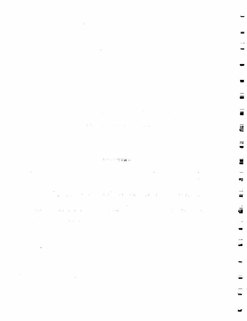
Fig. 1. Diagram sketching Strong, Weak and Variational Forms, and
relationships between form pairs. (Weak Forms are also called
weighted-residual equations, variational equations, Galerkin
equations and integral statements in the literature.)
A PVP is most useful from the standpoint of applications if the value of the functional,
evMuated at an extremal, is independent of the free parameters. This value has often the
meaning of energy. Such a principle will be called an invariant parametrized variational
principle or IPVP. The example functional (3) yields an IPVP if [u"(b)] 2 = [u"(a)] 2 or
if [u'(b)] 2 = [u'(a)] 2. (To prove the latter, insert u = -u" into HG and integrate.) If
[u(b)] 2 = [u(a)] 2, II is independent of fl for any u(z), not just an extremal. This will be
called an absolutely invariant PVP, or AIPVP.
The most useful IPVPs and AIPVPs, however, are those in which invariance does not
depend on boundary conditions. Such functionals will be encountered in following sections.
3.4 Connections with the Inverse Problem
The study of single-field PVP's constitutes a particular topic of the Inverse Problem of
Variational Calculus: given a system of differential equations -- herein called the Strong
Form or SF -- find the Lagrangians that have that system as Euler-Lagrange equations.
These Lagrangians (if they exist) collectively embody the Variational Form (VF) of the
problem. The Weak Form (WF) of the problem, which is also known by the alternative
names listed in Figure 1, is an intermediary between SF and VF. Relations between SF,
WF and VF are annotated in Figure 1.
4
I
I
I
u
w
l
U
w
w
U
w

w
9
m
w
m_t
L_
The Inverse Problem linking ordinary differential equations to single-field functionals is
treated in several monographs [55,57,62]. On the other hand, the multifield case is much
less developed. Aside from the developments presented here, parametrized functionals
have also been studied by the Beijing sch-ooi [37,38] but without establishing connections
to the Finite Element Method.
4. MULTIFIELD VARIATIONAL PRINCIPLES
Single-field PVP have limited practical and theoretical value. After all, gauge functions
have been known for a long time but never attracted much attention. Multifield (mixed)
PVPs are more interesting and fruitful, both theoretically and practically. In this section
two examples are worked out to unveil the flavor of the more complicated cases and expose
the reader to the notational conventions used in following sections.
4.1 One-Dimenslonal Example
As our first encounter with a multifield PVP, the following 6-coefficient generalization of
(2) to two independently varied fields: u a_nd p = u', is postulated:
b U b
II(u,p;J) = ½ u' |j12 J22 j2a u' dx = ½ zTJzdx,P L313 j23 j3z P
(8)
in which
Z = U I , J = 12 j22 j23 (9)
P L313 j23 j33
are the generalized field vector and the functional generating matrix, respectively. This
parameter matrix -- tlie "kernel" of the quadratic form in the z vector -- may be taken as
symmetric because only its symmetric part participates in the first variation. This general
notational arrangement is followed in more complicated linear problems of mathematical
physics presented later.
The Euler-Lagrange equations for _ii = 0 and ,_pII = 0 are
Eu : jllU d- j12u' + ji;P - (ji2 u' + j_2u" + j23)P' = O,(lO)
Ep : j13u + j23u' + j33P = O.
Consistency of (10) with the field equations u _ - p = 0 and u + p_ = 0 dictates that J be
of the form
.... :'! : : _J 0 -a (11)
--O_ OL
Thus the functional is found to depend on two independent free parameters: a and ft.
is this PVP invariant? At an extremal, p = u _, which replaced into (8) yields II =
1 f:(au 2 _ flu,2)dx. Therefore this is not generally an IPVP.
5

A more satisfying parametrization that automatically verifies invariance is obtained by
taking three independent fields, as in the example that follows.
4.2 A PDE Example: 2-D Isotropic Poisson's Equation
As second example we consider the isotropic Poisson's equation (the Laplace equation with
a source term) posed over a finite two-dimensional region _/bounded by a curve F:
kV2u = k _,Ox 2 -t- Oy2 ] -= -f in f_, (12)
where u = u(x,y) is the unknown function, k(x,y) > 0 and f(x,y) are given scalar
functions in f_. Boundary r is decomposed into p_, u rq, on which Dirichlet and Neumann
(flux-type) boundary conditions, respectively, are imposed:
Ou ^u=_ on F,, q=k_-_n=k(gradu)Tn= q on rq, (13)
where _ and _"are prescribed on ru and rq, respectively, and n is the exterior unit normal
on P. The single-field functional II(u) associated with (i2)and (13) is well known:
H=V(u)-P(u), U(u)=½ k "_x +\Oy,] jd , P(u)= fudf_+ , _udr.
(14)Here U(u) has the meaning of internal energy whereas P(u) is an external energy associated
with the source and prescribed-flux terms. As noted in Section 3.2, functional (14) can be
trivially parametrized by adding multiples of the divergence or rotor of gauge functions.
But such PVPs have no practical importance.
To begin the construction of a multifield PVP we introduce the two intermediate vector
fields: gradient g and flux vector p, as candidates for independent variation:
g= gyg_ =gradu= Ou/Oy , p= P_ =kg=kgradu=k Ou/oyOU/OX.
(15)The PDE (12) decomposes into the three field equations
g = Vu = grad u, p = kg, VTp + f = div p + f = 0, (16)
where ally -= V T is the divergence operator. In mechanical applications these are called
the kinematic, constitutive and balance equations, respectively.
The three field equations (16) and two boundary conditions (13) collectively make up the
Strong Form (SF) of the isotropic Poisson's equation. This SF is graphically represented
in Figure 2 using a modified Tonti diagram. Relations such as g = grad u are called
strong connections (which means that they are enforced point by point) and depicted as
solid lines. The main departure of Figure 2 from Tonti's original diagrams [47,59,60] is the
explicit separation of field equations and boundary conditions; this has been found useful
in teaching variational methods. In addition, a graphical distinction is made between
unknown and data fields, as indicated in Figure 2, also for instructional reasons.
=g
i
=
ZI
g
II
l
w
I
m
I

Ei•m
E
m_
Et
U
W
I ^nu: l.............U...............! on_ u
g = grad u
mr2
divp +f= 0
haf_
I IPkglgmo 0 IqpTn ton
I 1Unknown field Datafield
Strong connection
Fig. 2. Graphical representation of the Strong Form (SF) of the
isotropic two-dimensional Poisson's equation (12) with
the B.C.s (13) as a modified Tonti diagram.
4.3 A 3-Field PVP for Poisson's Equation
The configuration of (14) suggests trying to parametrize the internal energy U as a three-
field quadratic form, leading to the arrangement displayed below in full:
U(u,g,p)=½_
PM
kg,
kgy
k Ou/Oz
k Ou/Oy
"jxa jll j12jla jll j12j12 j12 j22j12 j12 j22j13 ja3 j23j13 j13 j23
312 313
312 313
J22 323
J22 323
323 333
323 333
313
313
323
J23
333
333
I k-lp.
k-lpy
g*
gy
Ou/OxOu/Oy
d_, (17)
in which for simplicity the explicit dependence of U on the j coefficients is dropped from
its arguments. The symmetry of the kernel matrix can be justified as in the previous
example, whereas its 2 × 2 block structure is a consequence of avoiding distortions in the
vector-component contributions to the internal energy. This functional is fully specified if
the 3 × 3 generating matrix J, which has the same form of (9), is given.
Now (17) looks unduly complicated for such a simple problem. At the same time, what
is being varied is not easily seen. We clarify and simplify this form in two steps: passing
7

I
to matrix-vector notation, and then applying the primary- versus derived-field convention
explained below:
U(fi, g, 15)- ½ [._ k_ j22I daJ_
k grad _ LJiaI j23I jaaIJ [ grad fi (18)
{ 15 }T [jnI j12I j131] {g P}g.._=½/aa Pg |j12I j22I j23I|df_.
pU LJ13I j2aI jaaIJ g_
Here I denotes the 2 × 2 identity matrix, pg = k_, p_ = kg" = k grad _, gP = k-l_,
g" = grad _. This notational convention, introduced in [19,20], is based on two rules:
1. A varied (primary) field is marked with a superposed tilde such as fi or 15. This allows
to reserve tildeless symbols such as u or p for generic or exact fields.
2. A derived (secondary) field is identified by writing its "parent" primary field as su-
perscript; e.g. p" = k grad _ is the flux associated with the varied field ft.
Of course at the exact solution of (12) all p's and g's coalesce, but the distinction is crucial
in variational-based approximation methods.
Note the pleasing appearance of the last term in (18): the notation groups fluxes on the
left and gradients on the right. Flux times gradient is internal energy, so the kernel matrix
simply weights, through the j coefficients, the nine possible combinations 15Tgp, _T_, ...
etc. (It is possible to further streamline (18) into U = ½ fn zTWz d_, as in the last of
(8), but this is too compact for most developments.) These notational conventions are
especially helpful in the more complicated application problems presented in Sections 5-7.
The first variation of U may be compactly expressed as
5U = Iv [(g)TSP + (_)TSg- (div _)TSu] dV + fs(p)Tn 5u dS, (19)
in which _, _ and _ denote the combinations
Z_ Z_ U
g=jllgP +j12g+j13g u, p=j1215+j22p° +j23p ", p=j1315+j23pg +ja3P u. (20)
On linking 5U with the variation of the parameter-free external-energy term P given in
(14), we obtain the Euler-Lagrange equations in _2
A _= =Ep:g=0, Eg: 0, E," div_+f 0, (21)
while the Neumann boundary condition on is (_)rn = _'. Consistency with the
three field equations (16) and the boundary condition q = _"leads to constraint conditions
on the j coefficients. These can be expeditiously obtained by noting that at the exact
solution of the Poisson's problem, p = 15 = pg = p_ and g = g = gg = g". Consequently
J11+ J12 + J13 = 0, Jll + J12 + j13 = 0, ja1+ j12 + j13 =1. (22)
8
mI
z
s
mm
I
g
W
m
im
.w
w
m
U
f
=
m
Im

L
===
w
It follows that the functional (18) combined with P yields a PVP, which is in fact a three-
parameter family. If we chose the diagonal entries jla, j22 and j33 as the free parameters,
the constraints (22) are met if the functional generating matrix takes the form
jn " I"7(-.hl -J22 +ja3 - 1) a •g(-311 + j22 -- j33 + 1) jll --s3
J = j22 i • [g(311 -- j22 -- j33 + 1) = -s3 j22
symm j3a --82 --Sl
--31 .
j33
(23)
Here the negatives of the three off-diagonal elements of J are abbreviated to sl, s2 and s3
for use below.
The choice ja3 = 1, others zero, yields the well known single-field functional (16). Other
choices for J are discussed in conjunction with the classical elasticity problem in Section
5, which has a similar parametric structure.
Using the decomposition of J as sum of rank-one matrices
000I!00 10i] 11!]J = 0 0 0 + S 1 1 -1 + s2 0 0 + s3 -1 1 , (24)
0 0 1 -1 1 -1 0 0 0
one can rewrite the three Euler-Lagrange equations (21) in a form that illuminates the
weighted-residual connection to the field equations (16):
E,: -g") + s3(gp = 0,E0: s3(p ° - _) + s,(p g p") = 0, (25)
E,: div [p" + sl(p" - pg) + s2(p" - 15)] + f = 0.
What happens if, say, s2 = s3 = 0? Then Ep becomes an identity and _ drops out as
an independently varied field [observe that jll = 0 because of (22) and consequently the
first row and column of J vanish.] Similarly if Sl = s3 = 0, Eg becomes an identity and
15 drops out as varied field. The case sa = s2 = 0 reduces E, to divp"+f = 0 but
three-field principles are still possible because one may select Jla = j22 = -j12 "- P, where
p is arbitrary; setting p = 0 gives back the simplified functional (14).
The form (25) show that the s's, or their reciprocals, can be interpreted as weights on
the field equations. No such flexibility is available with single-field functionals because
the parameters factor out at the first variation level. This is the key reason behind the
imp, ortance of multi field PVPs.
Is this PVP_invariant?. At an extremal the p's and g's coalesce. The internal energy
reduces to fa pTg dV multiplied by jll +j12 +... +jaa, which is one because of (22). Thus
we have an IPVP. The same property holds for all PVPs presented in Sections 5-8, and is
crucial in the application to finite element error-estimation discussed in Section 10.
Does (18) embed all: possible functionals for the internal energy of the Poisson's equation?
No[ In this formulation u must be a primary field in II, although 15 and/or g may drop
9

^
a ons u
e=Du
inV
DT+ f= 0
inV
A - - "
I I°: ele ° I -tl ! nin V on S t _,,.,...,....,.
il
m
t_
I
I
I
l
Fig. 3. Graphical representation of the Strong Form (SF) of the
primal (displacement-based) formulation of classicalelasticity. Refer to Figure 2 for display conventions.
out for certain choices of J as discussed above. To make u disappear, the last row (and
column) of J must have all zero entries, which contradicts the last of (22). Consequently
functionals with internal energy of the form U(p, g), U(p) or U(g) escape this framework.
This point is further elaborated in Section 5.5.
5. CLASSICAL ELASTICITY
"ClassicM elasticity" is short for the more precise "compressible linear hyperelastotatics."
This is the application area in which the multifield PVPs discussed here originated in
response to needs from finite element technology. As a result, it is still the best developed
one in terms of FEM applications.
Theensuing discussion emphasizes three-dimensionM eiasticity. Specialization to struc-
tural models such as beams, plates and shells, as well as the derivation of canonical func-
tionals for these cases, is covered from a modern viewpoint by several authors, e.g. Reddy
[53,54] and Hartmann [31].
5.1 Governing Equations
Consider an body of volume V referred to a rectangular Cartesian coordinate system xi,
i = 1,2, 3. The body is bounded by surface S of external unit normal n - hi. The surface
is decomposed into S' : Sd U St. Displacements d -- di are prescribed on Sd whereas surface
tractions t" = [i are prescribed on St. Body forces f - fi are prescribed in volume V.
The three unknown internal fields are: displacements u = ui, strains e = eij and stresses
o" - aij. The stress traction vector on S is o'n - an, = ajinj (summation convention
implied). To facilitate the construction of elasticity functionals in matrix form, stresses
10
I
W
"In
I
g
I
i
m
J
W

w
w
= ,
=__
w
w
m
m
and strains are arranged in the usual 6-component vector forms
o'T "-- [(:rll a22 (733 (712 a23 o'31 ] ,
eT--[ell e22 e33 2e12 2e23 2e31],(26)
These fields are connected by the kinematic, constitutive and balance equations
e = Du, a" = Ee, DTa • + f -- 0, (27)
where
D
O/OZl 0 00 Oax2 o
0 0 O/Oz3O/Oz2 O/Oz] 0
0 O/Oz3 O/Oz2OlOz3 0 Wax]
(28)
is the 6 x 3 symmetric-gradient operator, its transpose D T the 3 x 6 tensor-divergence
operator, and E is the 6 x 6 stress-strain matrix of elastic moduli arranged in the usual
manner. The boundary conditions are
u-d on Sd, a'.----t on S,. (29)
The field equations (27) and boundary conditions (29) make up the Strong Form (SF) of
the classical-elasticity problem. The SF is graphically represented in Figure 3 using again
a modified Tonti diagram of the primal (displacement-based) formulation.
5.2 Weak and Variational Forms
From the Strong Form one can proceed to several Weak Forms (WF) by selectively "weak-
ening" strong connections. A var!ation-homogenization and integration process then yields
a Variational Form (VF) as was sketched in Figure 1. Two specific functionals of classical
elasticity are worked out as examples before proceeding to the general parametrization.
Figure 4 depicts the Weak Form (WF) of the Potential Energy (PE) functional for classical
elastostatics, in which the displacement field u is the only primary field. The WF diagram is
adapted from the Strong-Form Tonti diagrams of Figures 2±3, with some additional graphic
conventions explained in Figure 4. Furthermore the derived field notation introduced in
Section 4.3 appears again. For example, e" = Du is identified by the "tracer superscript"
u that remind us that these are displacement-derived strains.
Two strong connections: the balance equations DTo " + f = 0 in V and the flux boundary
condition: o'_ = t" on St, have been weakened by making them satisfied only in an average
sense: ' ::_ "
Jv/(DT°'_' + f) w dV + Js/ (°'_' - t)w clS = O, (30)
11

A
fA ° l ° IeU= D
Varied (primary) field
Data field
I Im
_\\\\\\\\\\_q
Derived (secondary) field
Strong connection
Weak connection
U
J
Fig. 4. The Weak Form (WF) of the Potential Energy principle of classical elasticity.Also known as the Principle of Virtual Work. The function inner-product
abbreviations (a,b)v a_ef fv aTbdY and [a,b]s d__ffs aTbdS are used
for labeling the weak connections because f is not available for graphics.
where w are the "virtual displacements" in the parlance of mechanics. To pass to the VF,
set w = 6u, homogenize variations and integrate obtaining the Potential Energy functional
-- : : ...... -Assecond example, consider the:= -derivationof the Hellinger-Reissner=:= (HR)= stress-
displacement functional. Figure 5 depicts the appropriate Weak Form (WF). The varied
fields are displacements fi and stresses &. Three = =:=: :: _ .:-- _weaklinks have been introduced:......
/v(e _ -ea)6_dV +/v(DT_+ f)6udV + _s (&_ -t )6udS= O
..... where _e n _ _=_rijn j. From this one can pass to the Hellinger-Reissner functional
(32)
1-IHl_(fi,&)= /v&T(e_--½ea)dV--/vfTfadV-- fs tTfadS. (33)
: : :There are variants of both the PE and HR functionals in which the displacement boundary
condition u = ^d is only weakly enforced. This results in the appearance of an additional
Sd boundary term displayed in (35) below.
12
W
m
gmm
l--II_
m

• s
=
eU=D_
+=0
Fig. 5. The Weak Form (WF) of the Hellinger-Reissner principle of
classical elasticity. (For notation explanation refer to Figure 4.)
E-
l
m
==
--=
5.3 Canonical Functionals and Hybridization
The PE and HR functionals are instances of the so-called canonical functionals. According
to Oden and Reddy [46,47] there are seven canonical functionals for the primal formulation
of linear selfadjoint boundary value problems that fit the SF scheme of Figures 2 and 3.
For classical linear elastostatics these are listed in Table 1, along with the names of the best
known ones. (Oden and Reddy list eight functionals but one is a trivial combination of
PE and HR.) This number expands to 14 if one includes the dual formulation of elasticity
based on potentials, but such generalization -- which is discussed in detail by Oden and
Reddy [47] -- will not be considered here.
Are there more? The number increases if one allows hybrid functionals into consideration.
All functionals of classical elasticity can be expressed in the form analogous to (14):
II = U - P, (34): L : ::
where U is the volume term that represents stored strain energy and the potential P
includes body-force and boundary contributions. The conventional form of P is:
ec(fi, &, 6.) = fTfidV + (_r,,) (u d)dS + tTfidS.d c
(35)
13

U
Table 1. The Canonical FunctionaIs of Classical Linear Elastostatics
(after 0den and Reddy [47])
..... e :: =
Varied fields Acronym Functional name
i:! PE
& CE
6
fi, & HR
fi, _ SDRN
tr, e
u, ¢r, e HW
Potential energy
Complementary energy
No name
Hellinger- Reissner
Strain-displacement Reissner
No name
Hu-Washizu
g
!
J
where _r. is generally a weighted combination of o'", w e and _r as shown in Eq. (43) of
Section 5.4. The Sd term drops if the displacement boundary condition u = d is strong,
as in (31) and !33); in such case pc depends only on ft.
Two more forms appear when one considers hybrid functionals for a finite element dis-
cretization of V. (Such functionals can also be constructed for bodies with internal phys-
ical interfaces.) In the following Si is the counted-twice union of element interfaces not
on S, while (] and t are boundary-displacement and boundary-traction fields, respectively,
that are independently varied on Si:
Pd(fi,&,_,_l) -- fTfidV + (_rn) (u-d)dS + "_fidS + trT(fi-- d) dS. (36)d t i
Use of either of these potentials allows fi to be discontinuous across internal interfaces.
In (36) fields (] and fi are weakly connected on Si, whereas in (37) fields t and _,, are
weakly connected on Si. With these additional choices one can have, for example, three
variants of the Hellinger-Reissner functional: IICHR = UHR -- pc, IIdHR = UHR -- pal, and
IItHRd = UHR -- pt. The last two were called d-generalized and t-generalized function-
als, respectively, in [19,20]. The hybrid functionais of Plan and Tong [51,52,63] can be
precipitated as special cases of these two forms.
When these hybrid variants are accounted for, the number of primal canonical functionals
roughly triples (it is not exactly 7 x 3 = 21 because certain hybridizations are incompatible
with some functionals of Table 1). But in fact all of them are mere "points" in the space of
parametrized functionals constructed below. Therefore the correct answer to the previous
question is that there is an infinite number of functionals from which classical elasticity
can be derived.
I
al
mm
I
_=_
I
g
I
141
W

w
J22
w
=
J
w
_m
==
m
m
[-1 011.......HR/ooo /
" tlooj
0-11]HW-11o
100
ro::,i]/-101
L 1 1-1
J33
ooo]000001
_o
1
. [°°°1i SDR o-1 1
i 010
,o]1°o
"""_ J 11
Fig. 6. Representation of the three-parameter PVP for classical
elasticity in (j11, j_, jaa) space. Generating matrices
for interesting functionals are shown near the "points."
5.4 Heuristic Parametrizatlon
The strain energy portion U of II = U - P can be written down as follows for the PE, HR
and HW canonical functionals:
u_(_) = ½f. _" 0_r u 0
dV,
e u
(38)
'°!](e/=_l[,v _° 0 0UHR( _I, O') dV,tr _ I 0 e _'
1 o.e i I- o _ dV,UHW([I, a', e) = -_ or u I 0 0 e"
(39)
(40)
where I is the 6 x 6 identity matrix. This pattern suggests trying the parametrized form
U(u, cr,e) = 1 o-e
or u
Tj11I
j12I
jlsIj12i 1311j2zI j23I[ ejz3I j33IJ e u
dY. (41)
15

u
This is formally similar to (18) except that the or and e vectors have 6 components, and
the generalized field vectors 18 components.
The first variation of U can be compactly written
fv u T5U= [(_)Tsor+(_')TSe--(div_')TSu]dV+/(orn) SudS,,IS
(42)
in which _, _ and _" denote the weighted combinations
,, . eU .- ue= jl]e p + j]2_ + 2]a , or= j]2& + j22 org + j23 tru, Or= j]3& + j23 trg -4- j33or u,
Combining 5U with 5P yields 61-I. For example, if P is taken as pc of (35)
(43)
5II:/v [(_)TSor + (_.)T ,e_r T ,u] dV+ _ (_'. 't)TSudS+ fs (__fi)T 5_rn dS, (44)t d
where r = div or +f are internal equilibrium violations. Consistency arguments again show
that the coefficients must satisfy the constraints (22) reproduced here for convenience:
jll + j12 + j]a = 0, j12 + j22 + j23 0, j13 + j23 + j33 = 1. (45)
This leaves 6 - 3 = 3 free parameters. As usual the 3 x 3 matrix J of entries jkt is called
the functional generating matrix. The special settings
[i0!] 10i] [011 [!0i]J= 0 , J= 0 0 , J= -1 1 0 , J= -1 ,
0 -1 0 1 0 0 1
(46)yield the PE, HR, HW and SDR canonical functionals, respectively. Other interesting but
anonymous functionals in jl], j22, j33 space are marked with a o in Figure 6. A glance
at this figure derails the lofty status accorded the Hu-Washizu (HW) functional in many
textbooks as the most general three-field functional of elasticity.
The weighted field-equation representation analogous to (25) is
Ee: s2(e a - e u) + s3(e*' - _) = 0,
,3(or - + e - or")= o,E_: dlv [or_ + Sl(O "_ - ore) + s2(er_ _ &)] + f = 0,
(47)
where scaling factors sl, s2 and s3 are defined in (23). The general Weak Form for arbitrary
parameters is depicted in Figure 7. As can be observed this has become more complex,
requiring some study to sort out. The "strength" of the weak connections can be measured
by the value of the scaling factors as discussed in Section 4.3. If factor pairs vanish "box
merging" occurs as explained therein.
16
w
III
IB
i
W
m
=,=
U
I
F

!_aw
E_v
m
L__
I1
s 1
s 1
_////////////////////_
x_,\\\\\\\\\\\\\\\\\x_
Fig. 7.
Weak connections conjugate to 8o
Weak connections conjugate to 8e
Weak connections conjugate to 8u
Weak Form for the general parametrization (40). Numbers annotated
near weak connections are the scaling factors in Eqs. (46).
5.5 Functionals Without Independent Displacements
There is a subset of elasticity functionals without independently varied displacements; for
example the well known principle of Complementary Energy (CE). In Felippa and Militello
[22] it is shown that all functionals with independently varied stresses can be embedded in a
one-parameter form that includes CE as a special case. The only functional left out of these
three-parameter and one-parameter framework is the unnamed canonical functional whose
only independent varied field is strains. Summarizing: all canonical primal functionals of
linear elasticity can be covered with a 3-parameter family II(5, &, _), a 1-parameter family
H(5",_), plus a 0-parameter family II(_). This statement can be extended to encompass
hybrid variants.
5.6 Historical Note
The three-parameter form (41) was not the first one constructed. A one-parameter subset
that connects points PE and HR of Figure 6 was discovered in 1987 and published in
17

e=Du DTc+ f=O
s=Gg_I ° ° ...................Fig. 8. Generalization of the Strong Form of classical linear elastostatics
(diagramed in Figure 3) to encompass material incompressibility.
[19,20]. This was the byproduct of an effort to variationally justify the Free Formulation
(FF) of finite elements [12,13]. The effort was actually motivated by criticism of a follow-
up paper [18] by a reviewer who justly observed that the excellent performance of the
FF-based plate-bending element presented therein had computational but no theoretical
basis.
Subsequent developments were serendipitous. Another one-parameter form, joining
"points" HR and HW of Figure 6, had been constructed [40,41] to justify the Assumed
Natural Strain method [7,32,50,58]. This work evolved later into the Assumed Natural De-
viatoric Strain (ANDES) formulation [22,43]. Comparison of the SFF and ANDES results
led to the general parametrization (41) published in [22,23].
6. ENCOMPASSING INCOMPRESSIBLE BEHAVIOR
The functionals of linear elastostatics studied in the previous section fall if the material
is incompressible. To encompass incompressibility one must begin by splitting the stress
tensor into deviatoric and mean stresses, and the strain tensor into deviatoric and mean
strains. In Cartesian tensor notation:
aij = sij -P_ij,1
' eij = gij -- -_O_ij,
1p =-½aii = -_ trace er,
0 =-eii = -trace e = -div u.(48)
Here p denotes the (actual) pressure, 0 the total strain condensation, _ij is the Kronecker
delta, and the summation convention applies over the range 1,2,3. These tensor compo-
nents are arranged in 6-vector form following the prescription (26) so we can rewrite the
splitting (48) as
a=s-ph, e=g-0h, hT:[1 1 1 0 0 0]. (49)
18
II
W
I
g
J
u
FI
I
w
b
w

w
w
r__
E__
z
m
The kinematic relations and balance equations are stili e = Du and DTo " + f = 0 as
in (27). The boundary conditions are still (29). As far as the constitutive equations is
concerned, the assumed split is
s = Gg, p = k_, (50)
where (_ is a (generally anisotropic) deviatoric-stress-to-deviatoric-strain matrix inver_ible
for all values of compressibility, and k is thrice the bulk modulus K. Incompressibility
occurs in the limit k ---* c_. Note that the model (50) assumes that the material is
volumetrically isotropic although deviatoric anisotropy is permitted. The Strong Form
diagram shown in Figure 8 summarizes the governing equations.
The governing functionals are again II = U - P. The internal energy U has been
parametrized by Felippa [24] in the form
p,g,O)= ½fv
, T
S g
S u
pe
, pu
j11I ]12i jl3I jl4h jl_h jlsh-
j12I i22I j2aI J24h j25h j2_h
j13I i2aI jaaI ja4h ja_h j36h
j14h T j:4h T js4h T j44 j45 j46
jlsh T j:sh T jash T j45 j55 js_• T
.316h j26 hT ja6 hT j46 j56 j66
¢ gS '
g
g"
6p, dY,
(51)
where I is the 6 x 6 identity matrix, h is defined in (49), and the derived fields are
sg = G_, s" = G-1Dfi, p0 = kg, p" = -k div fi, g_ = G_, g_ = GDfi, OP = k-1i5
and _' = -div ft. In the incompressible limit OJ' vanishes. The analysis of [24] shows
that consistency of the Euler-Lagrange equations with the field equations requires that the
following nine constraints be satisfied:
jll +jl2nUjl3----0, j14"{-jls+j16----O, j12+j22-J-j23=O,
j24+j25+j26 =0, jla+j2s+js3 = 1, ja4+jas+j36=O,
j4_+j_6+j68 = 1, j44+j45+j46 =0, j45+j_+j_ =0.
(52)
Furthermore, to include the incompressible limit, j_ = j_ = 0. Consequently there are
21 - 11 = 10 free parameters. The s_mt)lest generating matrix that satisfies all constraints
J
j_
.?12
_14
J16
_12 _13
_22 _23
_23 _33
_24 Ja4
J26 _36
is
J14 j15
_:4 j:_
)a4 ja_
_44 j4_
_4_ j_
_46 j56
j16 "
J:_
ja_
j4_
j_
j_
-0
0
0
0
0
0
0 0 0 0 0
0 0 0 0 0
0 1 0 0 0
0 0 -1 0 1
0 0 0 0 0
0 0 1 0 0
(53)
This leads to a generalization of the PE functional (31) that exactly accomodates incom-
pressibility. Other choices are examined in [24], where stress-strain splittings more general
than (48) are considered.
19

Iu=dU
#I II
II
-1\
x=CTT (a=Ee, s=G¢) [
II
U
+
3
^
_n= t
Strong Form diagram for micropolar elastostatics without couple stresses.
7. MICROPOLAR ELASTOSTATICS
The extension to a if-nearly elastic micropoi_ medium without couple stresses has been
investigated by Felippa [25]. In this elasticity model the stress tensor 7"and the strain tensor
3' are no longer symmetric. They are decomposed as 7" = o" + s, and 3" = e + ¢, where _r
and e are the symmetric parts and s and ¢ the antisymmetric parts, respectively. (Symbol
s does not have the meaning of Section 6.) General, symmetric and antisymmetric tensors
that arise in this model may be arranged as 9, 6, and 3-component vectors, respectively,
to facilitate the use of matrix notation in the parametrized functionals. Notational details
are given in that reference.
The rotational portion of u now enters the field equations. The infinitesimal rotation
vector (also called macrorotations) is w = Ru, where R is the rotor or curl operator.
The microrotation vector 0 is introduced so that the antisymmetric strains are given by
¢ = w - 0. The irrotational part of u is ue, which generates the symmetric strains
e = Du = Du¢, where D is again the symmetric gradient operator. Finally, body-volume
actions are decomposed into f = b + c, where b and c are the body force and body couple
per unit volume, respectively. Classical elasticity is recovered if c vanishes.
The balance equations are DTer + f = 0 and RTs + c = 0. The constitutive equations
are er = Ee and s = G¢, which may be merged as r = C3", where C is block diagonal.
These field equations, plus the boundary conditions u = d on Sd and 7-,, = t" on St, are
summarized in the Strong Form diagram of Figure 9.
The functional II again decomposes into U - P. The parametrized form of the internal
2O
I
k _
M
m
11
U
g
il
lira
J
i
m
L_

l,
v
r.-
.==.
t_m
energy U has the structure
O"
O.e
Or u~
S uO
T-j1116 j1216 j1316 0 0 0
j1216 j2216 j2316 0 0 0
j1316 j2316 j3316 0 0 0
0 0 0 j4413 j4513 j4613
0 0 0 j4513 j5513 j5_I3
0 0 0 j4_I3 j5_I3 j6_I3
'ea ]e _e~
¢/ i ' dV,¢, ¢u0
(54)where Is and I3 denote the identity matrices of order 6 and 3, respectively. The derived
quantities are o"e = E_, o"u = ED£,, s ¢ = G¢, s ue = G(Rfi- 0), ¢_ = G-_ and
= -
The zero entries of the kernel matrix in (54) reflect the orthogonality of symmetric and
antisymmetric parts. The analysis carried out in [25] shows that consistency with the field
equations requires that
jll-{-j12-{-j13 =0,
jas-I-j45+j46 ----0,
j12 q-j22 + j23 = 0,
j45 q-j55 + j56 - 0,
j13+j23+j33=l,
j4_+j_+j6_= 1.
Consequently there are 12 - 6 = 6 free parameters in (54).
generating matrix that meets these constraints is
(55)
One possible choice for the
J _____
jll J12 Jla 0 0 0
j12 j22 j2a 0 0 0
jla j23 jaa 0 0 0
0 0 0 j44 j45 j46
0 0 0 j45 jss j56
0 0 0 j46 j56 j_6
--1 0 1 0 0 0
0 0 0 0 0 0
1 0 0 0 0 0
0 0 0 --1 0 1
0 0 0 0 0 0
0 0 0 1 0 0
(56)
An alternative application of these functionals is to non-polar media in which c = 0
although the symmetry of the stress tensor is only enforced weakly. Such functionals
furnish a basis for construction of finite elements for classical elasticity with independently
varied rotation fie_lds, a subject that has recently been given impetus by the paper of
Hughes and Brezzi [33]. In fact the choice (56) yields one of the canonical functionals
derived in that paper. The Appendix of [25] extends these PVPs to micropolar media with
couple stresses.
8. ELECTROMAGNETODYNAMICS
As final example, consider classical electromagnetodynamics based on Maxwell's equations.
In this model the unknown internal fields are the magnetic and electric fluxes H, and D
the magnetic and electric intensities B and E, the magnetic potential A and the electric
potential (I). The prescribed volume fields are the current intensity j and the electric source
21

Fig. i0.
II
L
I!
Q.
II
,m
"_ D=EE E
B =_H
II
|
mmt_.
P !L II
The Strong Form of isotropic linear electromagnetodynamics, withboundary conditions omitted for simplicity. Here e and # denote
the electric permittivity and magnetic permeability, respectively, ofthe medium. Other symbols are defined in the text. A superposed
dot denotes derivative with respect to time t.
I
u
I
U
I
U
l
I
p. The field equations are summarized in the SF depicted in Figure 10, in which boundary
conditions have been omitted for simplicity.
The general functional has the form II = U - S - B, where U is the generalized elec-
tromagnetic energy, S includes source terms and B contains boundary-closure terms. A
parametrized form of U studied by Felippa and Schuler [28] is
'LU=_×
C_ 1 i_i
c-lH B
c-lH A
f)t D E
D CA
T "gllI
g12I
g13I
g14I
g15I
.gl_I
g12I g13I g14I g15I g16I
g22I g23I g24I g25I g26I
g23I gazI g34I g35I gz6I
g24I g34I g44I g45I g46I
g25I g35I g45I g55I g56I
g2_I g36I g4_I gb_I g66I
IcB
cB A(57)
where I is the 3 x 3 identity matrix and c is the speed of propagation of EM disturbances.
(The parametrization coefficients for this functional are denoted by g instead of j to avoid
confusion with the symbol for current density.) The derived terms in (57) are H s = #-113,
H A = #-1 curl .A., D E = eE, etc. The analysis of [28] shows that the g coefficients must
22
J
W
I
W
1
W
g
1
W
L
m
=--
=,--
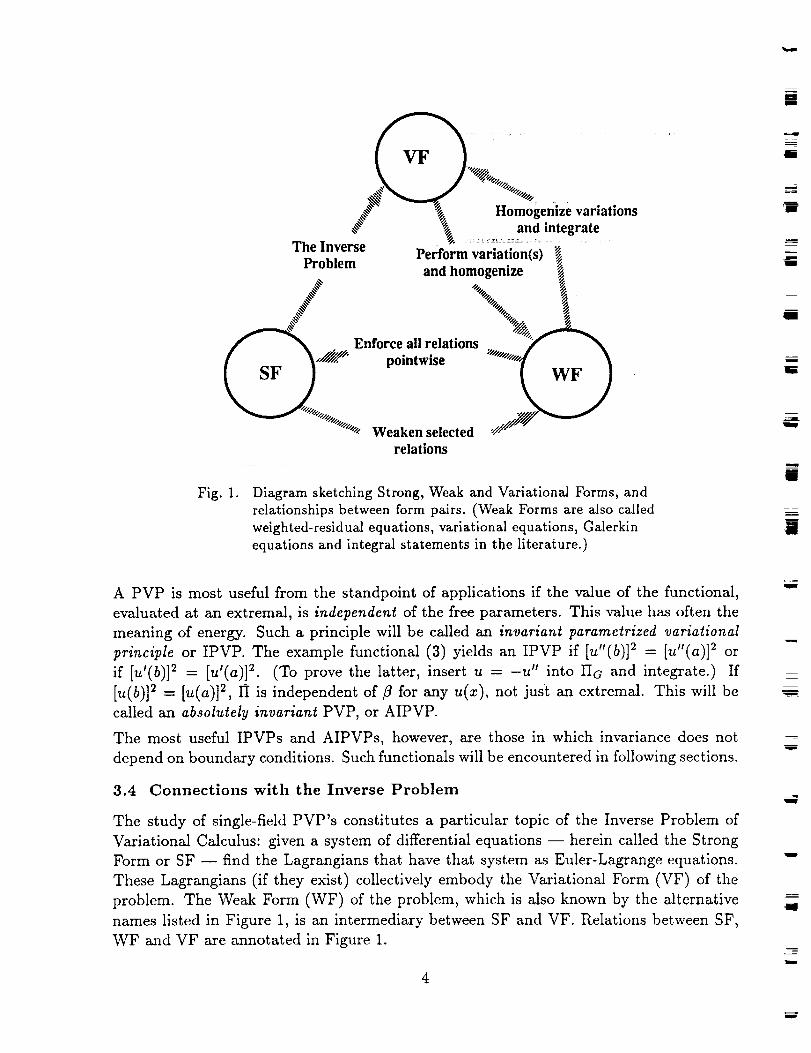
satisfy the 12 consistency constraints:
gll +g12Wg13 =0,
g12_g22_g23 =0,
g13+g23_g33 = 1,
g34+g35+g36 =0,
g14+g24+g34 =0' _
gls+g25+g35
g14-]-g15-{-g16 =0,
g24-{-g25+g26 =0,
g16]-g26-}-g36 =0,
g46+gs_+g_6 = "1,
g44+g45+g46 =0,
----0, gas+g_5+g56 =
which leaves 21 - 12 = 9 free parameters. The simplest choice for
G
g_ g12 g13 g14 g15 g_
g_2 g22 g23 g2a g25 g2s
g13 g23 g33 g34 g35 g3s
g_4 g24 g3t g44 g45 g4s
g_5 g2s g35 g45 g_5 gss
0
0
0
0
0
0
(5S)
,
the generating matrix is
0 0 0 0 0
0 0 0 0 0
0 1 0 0 0
0 0 0 0 0
0 0 0 0 0
0 0 0 0 -1
(59)
which, on including prescribed sources p and j, yields the two-field Lagrangian
½ - llV × XII v& ÷ _jT_ _ p_ dVdt. (60)
Felippa and Schuler [28] extend this PVP to the situation in which the current density j
is unknown, in which case Ohm's law has to be adjoined to the governing equations. This
extension is important as a departure point for the finite element analysis of Type I and
II superconductors.
9: APPLICATIONS TO FINITE ELEMENT METHODS
From previous examples it is seen that multifield PVPs are interesting in their own right
because they provide a continuous space of functionals. Canonical functionals are "instance
points" of this space. Moving in this space is equivalent to changing weights on the field
equations. A theorem proven for a parametrized functional is "economical" in the sense
that it need not be redone for specific instances.
Traditionally books dealing with applications of variational calculus in mechanics jump
from one specific canonical functional t0another. This approach has two instructional
disadvantages. First the reader is left with the impression that only a finite number of
functionals exist. Second, what ought to be shared properties are proved over and over, a
boring repetitive feat that can easily span hundreds of pages.
Aside from this theoretical and educational unifying value, multifield PVPs offer applica-
tions to variationally-based methods of approximation in general and the Finite Element
Method (FEM) in particular. Following are three intriguing subjects pertaining to FEM,
which in the author's opinion merit further exploration.
23

m
(A) Improved Approximation. Approximate FEM solutions generally depend on the
free parameters while the converged solution (assuming a convergent approximation
method) does not. Can the parameters be chosen to improve the quality of approxi-
mation on a fixed finite element mesh?
(E) A-posteriori error estimation. Assume the PVP is an IPVP. Suppose we obtain FE
solutions for two different parameter sets on the same mesh. As the mesh is refined the
values of the functional for both solutions approaches each other over each element.
Can this property be exploited to construct local (element level) error estimators?
(T) Templates. Using PVPs, can we derive universal "templates" for FE matrix expres-
sions that covers all convergent finite elements of a given freedom configuration?
The answers to these questions are in different state of development.
Exploiting (A) leads to high-performance finite elements. This is an application that has
been investigated over the past four years with focus in classical elasticity, and has led
to production-level finite elements. Knowledge as to the effect of parameter selection is
increasing, but much remains to be done.
Exploiting (E) leads to element-level error estimators. Only limited numerical experimen-
tation has been carried out, and most of the theory remains to be developed.
The idea of templates (T) has been explored for some specific finite elements, but it remains
largely a conjecture.
The next three Sections describe the state of these applications in further detail.
IO. APPLICATION 1: HIGH PERFORMANCE FINITE ELEMENTS
A high performance finite element (HPFE for short) for structural mechanics is a simple
element that delivers results of engineering accuracy on coarse meshes.
By "simple" it is meant that the element has few degrees of freedom, all physical, preferably
at corners only. Engineering accuracy typically means less than 1% error in displacements
and 5% in stresses. The term "coarse mesh" is subjective. In terms of structural applica-
tions, it characterizes a mesh that an experienced modeler would use to capture the basic
physics with a minimum number of degrees of freedom. This number is of course problem
dependent: a coarse mesh for a simple supported, uniform loaded plate would typically be
a 2 x 2 or 4 × 4 mesh with less than 100 freedoms; on the other hand a coarse mesh for a
complete aerospace vehicle may involve 50,000 to a million freedoms.
Mandatory attributes for a HPFE are: convergent, frame invariant and rank sufficient.Desirable attributes include:
• Yields similar accuracy in displacements and stresses.
• Is relatively insensible to geometric distortion.
• Is mixable with other elements.
• Provides effective a-posteriori error estimators to drive mesh adaptation procedures.
24
I
g
m
l
U
i
g
im
g
i
F
_ I
w
W

M.*
r_
w
m
L _
zm
E_,,_
B
• Fits naturally into displacement-based FE programs.
• Extends readily to nonlinear and dynamic problems.
The goal of attaining reasonable accuracy with coarse meshes of simple elements is the key
one, however, and deserves further comment. This requirement should not be confused with
fast asymptotic convergence for fine mesheSi= Simple elements cannot effectively compete
with higher order elements in this regard, and are not effective in applications that demand
very high accuracy. What matters is the accuracy obtained for the meshes typically used
in complex engineering systems, as discussed above.
10.1 Unification
Many tools and techniques have been developed over the past three decades to develop
HPFEs. The most practically important are: (a) incompatible shape functions; (b) hybrid
and mixed formulations; (c) reduced, selective and directional numerical integration; (d)
assumed natural strains and the Free Formulation. These four techniques originated in
the mid 1960s, late 1960s, early 1970s and early 1980s, respectively.
The approach recently pursued by the author has relied upon the use of PVPs with hybrid
treatment of element interfaces. More specifically, three ingredients are used:
1. The parametrized internal energy functional (41).
2. A d-generalized hybrid treatment of interfaces through the forcing potential (36).
3. Additional assumptions (sometimes called "variational crimes" or "tricks") that canbe placed on a variational setting through Lagrange multipliers.
The first two ingredients says that HPFEs can be effectively constructed using hybrid
PVPs of the form
IIa(5, &, _, c]) = U(5,&,_) - Pd(5,&, _, _]), (61)
where U and pd are given by (41) and (36), respectively. Observe that pd contains indepen-
dently varied displacements c] on element interfaces. This allows the internal displacements
fi to be nonconforming and in some cases (ANDES elements) ignored entirely.
Throughout this section we shall deal with individual elements only. Element identifiers,
which will be required in Section 11, are omitted for simplicity.
For mechanical elements modeled by classical elasticity, the HPFE derivation method
summarized in Figure 11 leads to finite element stiffness equations that decompose as
(Kb + Kh)v = p, (62)
where v are visible degrees of freedom (those matched with other elements, also known
as connectors), p are associated node forces, Kb is the basic stiffness matrix, which is
constructed for convergence and mizability, and Kh is the higher order stiffness matrix,
which is constructed for stability and accuracy. This decomposition was first obtained,
without variational arguments, by Bergan and Nyg£rd in the derivation of the unsealed
Free Formulation [12]. A key result of the multifield variational formulation is that only
Kh depends on the functional parameters [22,23].
25

Element Basic Higher Order
db dh
i!. +
_,SFF,EFF)
(ANS,ANDES)
Fig. 11. Summary of assumptions made in constructing a high-performance mechanical
element from the PVP (61)' For the basic stiffness an interior constant stress
field & = & and an interelement-compatible boundary displacement field (tb are
assumed. For the higher order stiffness either an internal displacement field fi
is assumed with the FF and its variants, or an internal strain field 6 is assumed
with the ANS formulation and its variants. (Only the deviatoric part of
appears in the ANDES variant.) The boundary displacement field (th need
not be the same as rib, although it often is. In the FF and variants thereof,dh and fi are collocated at node points.
10.2 The Parametrized 3'Node Bar Element
The 3-node bar element depicted in Figure 12 will be used to illustrate the steps in the
derivation of HPFE stiffness equations from PVPs. The element has total length 2h
and constant axial rigidity EA. The applied force per unit length is f(x). The internal
fields are the axial displacement u(x), axial strain e(z) = u'(x), and internal axial force
N(x) = Aa(x) = EAe(x). The 3 degrees of freedom (dof) are the node displacements v,,
v2 and v3 along the bar axis. For an internal finite element of this type, the d-generalized
parametrized functional (61) reduces to
N _ -sa j22 -sl _ dx- fudxIId(fi'N'_"d)=½ h N _, -*2-sa j33 e" h
(63)
LI
where N e = EA_, N u = EAu', e N = (EA)-IN, e u = u', and N= -s21V - siN _ +333" N u.
To construct the element we make assumptions on the varied fields N, fi, g and d. In
expressing _ and _ it is convenient to introduce the hierarchical displacement of node 2:1
732 = v2 - 7(Vl + va), which is the midpoint deviation from linearity. We also introduce
the natural coordinates (1 = ½(1 - x/h) and (3 = ½(1 + x/h) for convenience.
26
,umt
i
J
i
II
U
I
!
It
zm
g
zII
J
u
i
w
U
m

= ==__w
.e*.:.]_: ,_t. j
,#_i|i,'_
d(-h)
Oi i i i
EA--
/ 3 -- v3.... "---'-'"-'---_---"*---'--'*-'--'---'*-f(x)
Fig. 12. Three-node bar element used a.s example of derivation of
stiffness equations from the d-generalized principle (63).
N
==
w
IL_
-_._.u
=
The internal force is constant over the element: N = fig. The mean force N is a degree of
freedom that (thanks to the hybrid treatment) can be eliminated at the element level.
The axial displacement is expanded into a basic (linearly-varying) component ub, which
represents rigid body modes and constant strain states, and a higher-order (quadratically-
varying) component uh:
(z(x) -- ub(x) + Uh(X), Ub(X) -- Vl_l + V3_3, Uh(X) = 4_2_1_3. (64)
The assumed strain is also split into a basic component (the average or mean strain 5) and
a higher-order component called the deviatoric strain:
e=eTeh, e=(va-Vl)/h, en(z) =-_--[# sign(z)- 2(1- #)], (65)
Observe that eh is represented here by a constant-plus-linear function that is odd in x, and
contains a coefficient # that weights the "mixing" between the constant and linear parts.
If # = 0 the strain varies linearly as in the quadratic-displacement element and _ = e _'.
If # = 1 the strain is constant over subelements 1-2 and 2-3 and agrees with that of the
"macroelement" constructed with two linear 2-node bar elements. The assumption (65)
satisfies the compatibility conditions f° h ca(z)dx = - f: eh(X)dx = _2 for any/1.
Finally, the boundary displacements are identified with the end-node displacements:
d(-h) = a -h = d(h)= d h = (66)
Because u(z) also agrees exactly with vl and va at the end nodes, the boundary term in
(63) vanishes. Inserting the above assumptions into (63) produces a quadratic form in
the degrees of freedom vl, _52, v3 and fig. Rendering the form stationary with respect to
27

these freedomsleads to a system of linear equations that immediately gives N = EA_ =
EA(v3 - Vl)/h. Elimination of N yields the element stiffness equations
01]1 0 _ 2EA
o o-1 0 oool){vl} {pi}0 1 0 _2 = /)2
0 0 0 v3 P3
(67)
where forces Pl, i52 and pa result from the nodal lumping of f(x) and
1 1 2f_= _[(4--#)j11+(# 2 #)J22+#j33+(4--#)]= + +(#2 2#+ +- - 4)s3 4]. (68)
Expressing (67) in terms of the total midpoint displacement v2 rather than 7)2 yields
EA
6h
1 0
0 0
-1 0
3+3/3
-6/3-3 + 3/_
: :-: :: 7 7 :
-1 EA [I -2
0 L- 2 41 -2
{vi}-6_ 3 v3
1){vi}-2 v2
1 v3
{Pl /
-- P2 •
P3
(69)
Here we see the emergence of the stiffness decomposition (62). The basic stiffness Kb
contains no parameters and has rank one, so by itself it is rank deficient. The higher order
stiffness has also rank one and its addition stabilizes K as long as/_ > 0.
Although the FEM solution converges for any positive/_, maximum accuracy in smooth
problems is obtained for /_ = 4/3. This yields the well known 3-node quadratic bar
element. [To check this, take ja3 = 1, jll = j22 = 0 in (68) to get the PE functional, which
annihilates the separate strain assumption (65).] On the other hand, setting/3 = 1 yields
the 3-node "macroelement" equivalent to assembling two linear bar elements. [To check
this, take j22 = 1, jll = ja3 = 0 in (68) to get the HW functional and set/_ = 1].
The foregoing derivation appears to be overkill for such a simple element. Indeed (69) can
be obtained without recourse to any variational principle. Direct physical reasoning (as in
the original FF), algebraic arguments relying on subspace decomposition of node motions,
or even finite differences: all methods lead to (69). Such universality is the motivation
behind the template conjecture discussed in Section 12. In two and three dimensions and
especially complicated elements, however, variationally-based methods do have a place.
10.3 The Parametrized 2-Node Plane Beam Element
As a second one-dimensional example consider a two-node element for an Euler-Bernouilli
(C 1) plane beam of constant rigidity EI and span h. The four nodal degrees of freedom
are the transverse el_d displacements wl and w2 and the end rotations/_1 and 02 as shown
in Figure 14. Any parametrization method, whether variationally based or not, produces
28
g
J
w
W
m
g
i
U
W
i
i

w
L_
=__
m
=__
=__
w I
Z,W
EI
01
Fig. 13. Two-node Euler-Bernouilli beam element.
a decomposed stiffness matrix of the form
I!°°000°1EI 1 0 -1 EI
K = Kb + Kh = _ + j3--_-
-1 0 1
4 -2h -4 ]-2h
r-2h h 2 2h h 2
-4 2h 4 2h "
-2h h 2 2h h 2
(70)
where _ > 0. Both K_ and Kh have rank one, and combine to provide the proper rank of
two. The (optimal) Hermitian-cubic beam element is recovered if _ = 3.
An interesting property is that the Timoshenko (C °) beam has exactly the same stiffness
decomposition but the optimal _ is then 3 + 36(EI/GA)h -2, where GA is the section-
averaged shear rigidity; if GA ---+¢x_ or h ---+0, _ ---* 3. The distinction made in the copious
finite element literature on C o versus C 1 beam elements is seen to be artificial.
10.4 Three High-Performance Triangles
For multidimensional elements the general parametrized functional (61) has not been yet
exploited in its full generality. As of this writing only two one-parameter subsets have
been studied in some detail:
1. A stress-displacement d-generalized functional II_(fl, &, d) associated with the Free
Formulation (FF) and two variants thereof: the Scaled Free Formulation (SFF) in-
troduced in [13] and the Extended Free Formulation (EFF) proposed in [21]. Its free
parameter is called 7- Reduces to PE for "i' = 0 and to HR for 7 = 1 (see Figure 14).
2. A stress-strain-displacement d-generalized functional II_(u, er, e, d) associated with
the Assumed Natural Deviatoric Strain (ANDES) formulation. Its free parameter is
called a. Reduces to HR for a = 0 and HW for a = 1 (see Figure 14).
The most successful multidimensional HP elements constructed to date using these subsets
are depicted in Figure 15 and briefly described below. The EFFAND element is a plane
stress triangle (membrane component in shell element) with nine degrees of freedom, three
29
J22I
HW
_O _
"33 DSDR
Jll
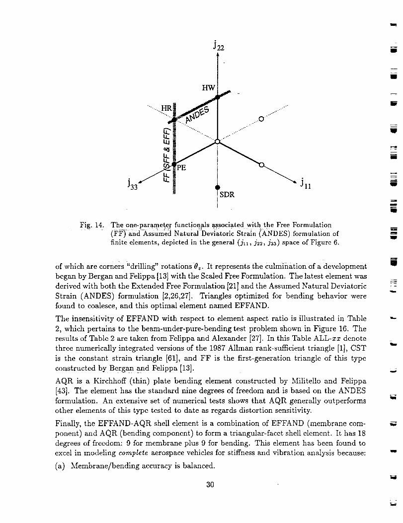
Fig. 14. The one-parameter functionals associated with the Free Formulation
(F15_and_ssumed Natu_rai_-Dev_atoric Stra{n (}kNDES) formulation of
finite elements, depicted in the general (j11, j:2, jaa) space of Figure 6.
of which are corners "drilling" rotations 8z. It represents the culmination of a development
began by Bergan and Felippa [13] with. the Scaled Free Formulation. The latest element was
derived with both the Extended Free Formulation [21] and the Assumed Natural Deviatoric
Strain (ANDES) formulation [2,26,27]. Triangles optimized for bending behavior were
found to coalesce, and this optimal element named EFFAND.
The insensitivity of EFFAND with respect to element aspect ratio is illustrated in Table
2, which pertains to the beam-under-pure-bending test problem shown in Figure 16. The
results of Table 2 are taken from Felippa and Alexander [27]. In this Table ALL-xx denote
three numerically integrated versions of the 1987 Allman rank-sufficient triangle [1], CST
is the constant strain triangle [61], and FF is the first-generation triangle of this type
constructed by Bergan and Felippa [13].
AQR is a Kirchhoff (thin) plate bending element constructed by Militello and Felippa
[43]. The element has the standard nine degrees of freedom and is based on the ANDES
formulation. An extensive set of numerical tests shows that AQR generally outperforms
other elements of this type tested to date as regards distortion sensitivity.
Finally, the EFFAND-AQR shell element is a combination of EFFAND (membrane com-
ponent) and AQR (bending component) to form a triangular-facet shell element. It has 18
degrees of freedom: 9 for membrane plus 9 for bending. This element has been found to
excel in modeling complete aerospace vehicles for stiffness and vibration analysis because:
(a) Membrane/bending accuracy is balanced.
3O
I
W
in
,==J
mqll
I
i
g
W
u
w

=
L •
E--
0zU Z
Uy Oy
Z
X
u X
• Li.:
Ozt
EFFAND-AQR x "_. , OX
0 X
Fig. 15. Three high-performance elements constructed with PVPs: the
EFFAND membrane 9-dof element, the AQR plate-bending
9-dof element, and the EFFAND-AQR 18-dof shell element.
(b) Global results -- e.g. frequencies -- of engineering accuracy may be obtained with
"coarse" meshes (for a complete aircraft, 50,000 to 200,000 dof). This is importantfor full-vehicle aeroelastic simulations.
(c) The presence of a complete set of rotational freedoms eliminates juncture modeling
problems.
(d) The element simplicity helps implementation on medium and fine-grained parallel
supercomputers with limited memory per processor.
11. APPPLICATION 2: LOCAL ERROR ESTIMATION
As second PVP application we take up the subject of a posteriori estimation of the local
discretization error of a computed finite element solution. These estimators may be used
to guide computer-driven mesh adaptation processes based on r, h or p techniques.
The theory of FE local estimation and mesh adaptivity has received substantial attention
over the past 17 years since the appear_ce of the original papers by Babu_ka [4] and
Sewell [56]. Much of the theory pertains to conforming finite element models based on the
Potential Energy principle or its equivalents. Because elements based on these assumptions
31

n
Y
32 - M=100
D
J
m
w
z
II
Fig. 16. Test problem for high-performance membrane element: 16:1
cantilever of rectangular cross section under pure end moment M.
Poisson's ratio v = 0, E adjusted so that exact tip deflection is100. A 32 x 2 mesli iS sh0wn. Each rectangular macroelement is
made up of four "crisscrossed" membrane triangles. (After [27].)
Table 2. Tip Defleciiona (exact=lO0) for Beam of Figure 16
g
lg
U
Element v Mesh: z-subdivisions x y-subdivisions
32x2 16x2 8x2 4x2 2x2
ALL-3i 0 87.99 75.47 37.01 5.51 0.42
ALL-3m 0 81.02 51.62 9.64 0.74 0.04
ALL-7i 0 85.43 67.44 23.65 2.55 0.17
CST 0 53.33 33.33 13.33 3.92 1.02
EFFAND 0 100.00 100.00 100.00 100.00 100.00
FF 0 100.25 99.15 98.38 98.08 97.98
are rarely the best performing ones, a curious situation arises in which the well developed
error theory applies to rather uninteresting elements., : :
11.1 Error Equations for Poisson_s Problem
We review the basic error equations for a conforming finite element discretization of the
Poisson's problem discussed in Section 3.2 based on the PE-like principle (14). The analysis
follows essentially Babu_ka and Miller [5] as well as Babugka, Dur£n and Rodriguez [6].
The bounded domain f_ with boundary F is replaced by a regular FE mesh with nonover-
lapping elements numbered e = 1,... N +. Element e has interior f_+ and boundary r _.
The latter is composed of N_ element sides identified as 1"3, j = 1,... N_e. For simplicity
the geometric discretization error is neglected so that f_ _-- UeF/e and 1-' - Ue,jF_ V F_ E F.
Further it is assumed that when an element side belongs to F, it is completely contained
32
J
I
w
gg
: =
J
II
I
= =
W

= =
T--!
L
w
w._.$
in either F_ or Fq. The union of element boundaries F_ not on I' is called Fi, which thus
collects all internal sides. An internal side that is shared by two adjacent elements e andd is called F _d.
Let u = u(x,y) be the exact solution of the Poisson problem (11)-(12) with f E L2(_),
_'E L2(Fq) andS'= 0onFd. Let _ = _(x,y) E HI(_) : Fa = 0 be a conforming finite
element solution, and eu = u - _ the approximation error. The localization of _ over
element e is _e. The source residual is r - V2_ + f in each fie and is conventionally zero
over element sides. For each element e we denote the boundary-normal flux derived from
as qU_ = kO£z*/On* where n _ is the unit outward normal on F _. On each internal side
Fed shared by elements e and d we select a common normal direction n ed and define the
flux jump as
_q,,,a] = q., cos(n*, n d*) - q,,a cos(n a, nd,), (71)
a value that is independent of the choice for n *d. Let w = w(x,y) E Ha(fl) : W[r'd = 0 be
a test function. Introduce the usual bilinear form associated with the internal energy (14)
U(u,w) = fn(div u) T div wdfl. (72)
On integrating by parts one finds that the error satisfies
V(u - fi, w) = U(e u , w) = fw dn + w dfl + dr - --w dr'e--1 ¢ ¢ e=l , One
= rwdn+ -er,q e,d
(73)which may be called the Weak Form of the Error (WFE). It displays three contributions.
The first term shows the effect of the source'residual error r = _72_ + f over each element.
The second term brings the effect of violating the flux boundary conditions. The third
term gives the contribution of interelement flux jumps.
The error energy measure is obtained by taking w = u - fi = e_:
Rde=f U(et"e') -- fn re" d_+ / (_'-q_')e u dr`- Efr Eq_'_d_e_' dr`, (74)q e,d *d El"/
which may be called the Error Energy Equation (EEE). Relations of this nature are the
basis for developing a posteriori local'err0r: estimators-for the Laplace and Poisson equa-
tions as well as (with suitable extensions) the Stokes and elasticity problems. There is an
abundant and rapidly growing literature in this topic. The state of the art is typified by
the research of Oden and coworkers [16,48,49].
Several technical difficulties, however, may be noted.
1. Both WFE and EEE involve the exact solution u, which is of course unknown. Con-
sequently a higher order estimation is inevitable. One way to achieve this is by
33

i
EA
u(x)
f(x)
Fig. 17. Bar problem used to illustrate behavior of HOE error indicator.
considering element patches (macroelements) and smoothing _, as in the widely used
projection method of Zienkiewicz and Zhu [67]. Another group of techniques relies on
hierarchical approximations [64,65,66].
2. Many interesting problems display jumps (e.g. at shocks, wavefronts, plastic bands)
in the exact solution. The resulting lack of smoothness -- in the previous case, u can
be no longer assumed in H 1 (f_) -- requires substantial revisions in the analysis.
3. The FE solution has been assumed to be variationally consistent with Eq. (14), that
is, fully conforming. But in many practical problems, especially in structural and
continuum mechanics applications, interelement continuity is lost. This may be due
to several factors. First, as noted in Section 10 most high-performance finite elements
(HPFEs) abandon conformity from the outset. Second, the treatment of complicated
3-D structures such as shells, folded plates or stiffened panels often introduces discon-
tinuities even if the constituent elements (by miracle) were fully conforming.
4. Although a WFE such as (73) can be formally extended without difficulty to PVPs
thus fitting HPFEs, the resulting EEE is generally indefinite and thus unsuitable as
an error measure. It is preferable to keep error measures positive definite, as in the
example that follows, by concentrating on a single field of interest to the user.
11.2 The 3-Node Bar Element Revisited
To motivate the approach discussed below, it is useful to consider again the 3-node bar
element of Figure 11, now as the problem depicted in Figure 17. This example connects to
the Poisson's equation discussed above by simply taking k = EA, u as axial displacement,
and f as prescribed axial force. Domains f/and F reduce to x-aligned segments and end
node points, respectively. The bar ends are assumed fixed: Vl = V3 = 0; therefore _2 = v2.
End fixity is not an important restriction because any element must exactly capture the
linear motion ub of (64).
We investigate here an assumed strain element variant of that considered in Section 10.2.
It is based on the ANDES functional (already mentioned in Section 10.4) that is obtained
by taking jll = a - 1, j22 = a, j33 = 0, and which reduces to HW for c_ = 1 and to HR
for c_ = 0. The assumptions on N, _ and d are as before. The displacement field is again
34
m
L--
i
J
M
m
I
I
I
i
J
J
m
m
U
J
w
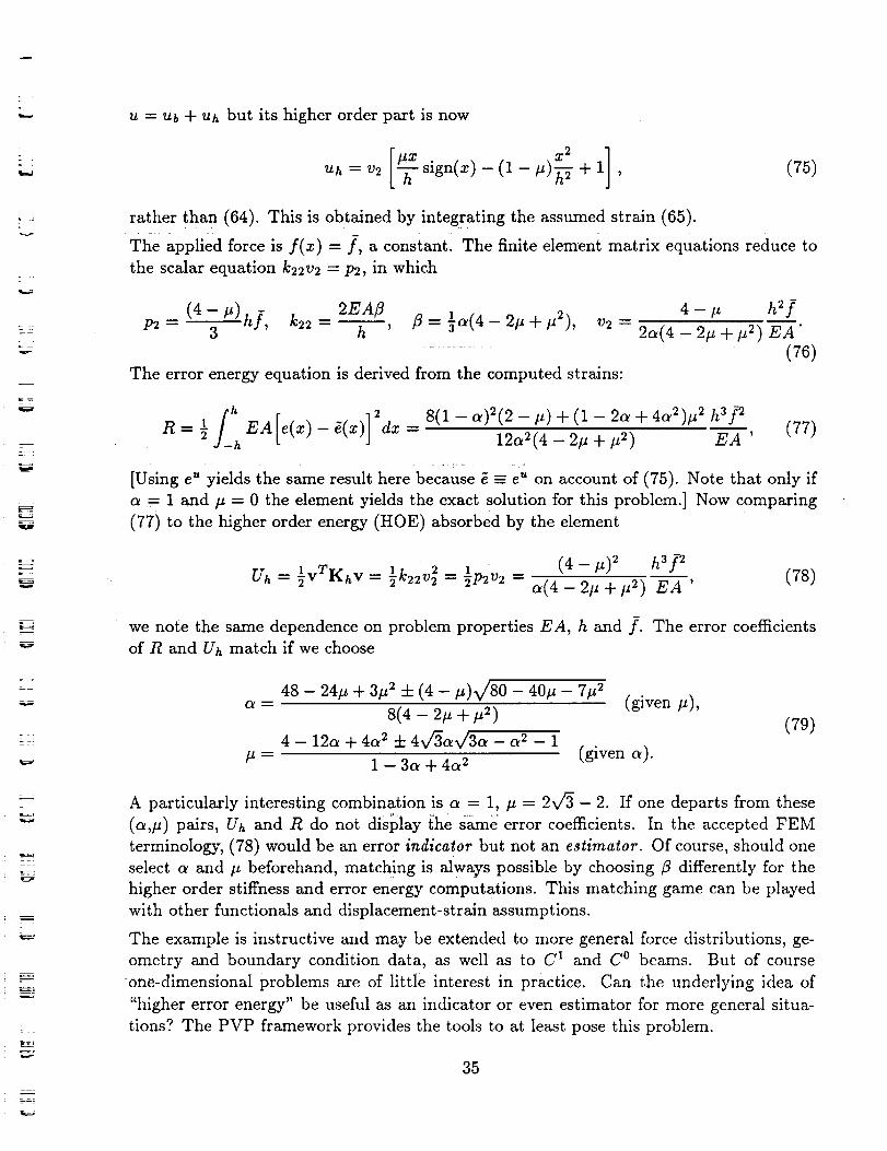
: ?
w
v
= =
L .
u = Ub + uh but its higher order part is now
Uh = v2 sign(x) -- (1 -- #)_- + 1 , (75)
rather than (64). This is obtained by integrating the assumed strain (65).
The applied force is f(x) = f, a constant. The finite element matrix equations reduce to
the scalar equation k22v2 = p2, in which
(4-_t) h], k22- 2EArlP2 -- 3 h ' fl = _o_(4- 2# + _2), V2 __
- 7
The error energy equation is derived from the computed strains:
4 - _t h2f
2a(4 - 2# + #2) EA"
(76)
F [ ]R=½ EA e(x)-_(x) 2dx=8(1-a)2(2-#)+(1-2c_+4a2)#2h3f2h 12a2(4- 2# + #2) EA '
(77)
[Using eu yields the same result here because _ e" on account of (75). Note that only if
a = 1 and # = 0 the element yields the exact solution for this problem.] Now comparing
(77) to the higher order energy (HOE) absorbed by the element
Uh ½vTKh v = 1 2 1 "= _k22v 2 = _p2v2 =(4-#) 2 h3f 2
c_(4 - 2# + #2) EA '(78)
we note the same dependence on problem properties EA, h and f. The error coefficients
of R and Uh match if we choose
48 - 24# + 3# 2 + (4 - #)_/80 - 40# - 7# 2
8(4 - 2_ + #2) (given #),
4 -- 12a + 4a _- :i: 4v/3a_/3a - a 2 - 1
1 - 3a + 4a 2 (given a).
(79)
A particularly interesting combination is a = 1, # = 2V_- 2. If one departs from these
(a,#) pairs, Uh and R do not display ihe same error coefficients. In the accepted FEM
terminology, (78) would be an error indicator but not an estimator. Of course, should one
select o_ and # beforehand, matching is always possible by choosing fl differently for the
higher order stiffness and error energy computations. This matching game can be played
with other functionals and displacement-strain assumptions.
The example is instructive and may be extended to more general force distributions, ge-
ometry and boundary condition data, as well as to C 1 and C o beams. But of course
one-dimensional problems are of little interest in practice. Can the underlying idea of
"higher error energy" be useful as an indicator or even estimator for more general situa-
tions? The PVP framework provides the tools to at least pose this problem.
35
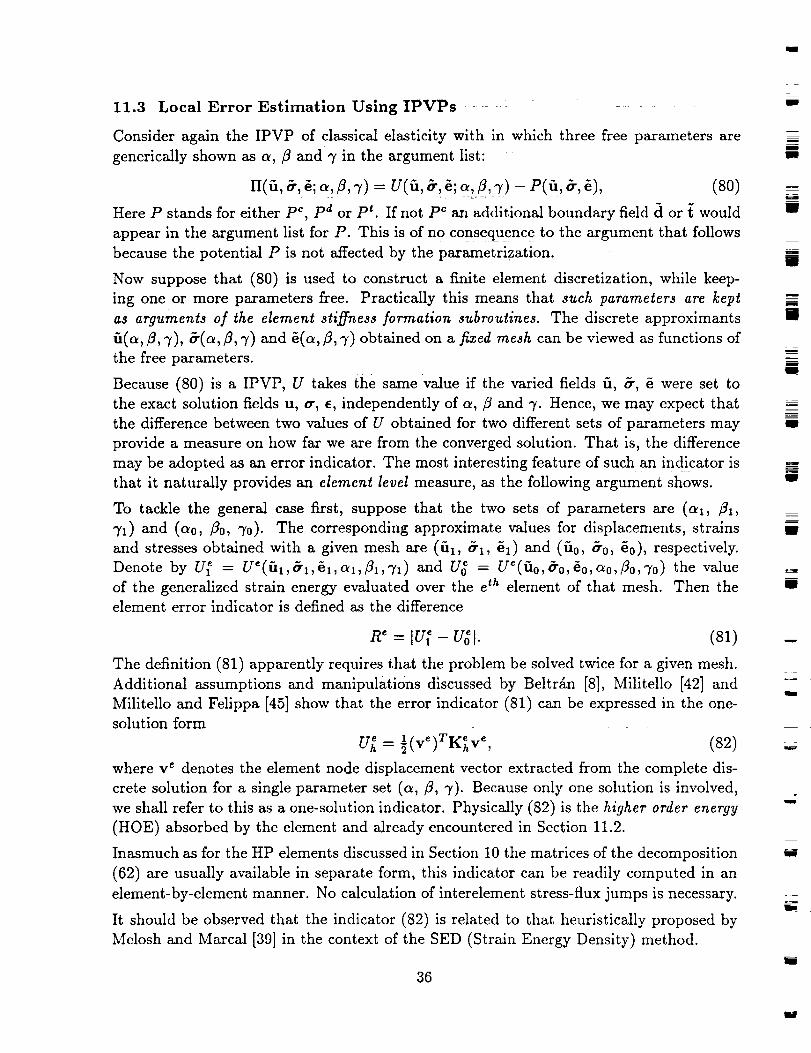
11.3 Local Error Estimation Using IPVPs
Consider again the IPVP of classical elasticity with in which three free parameters are
generically shown as a,/3 mad 7 in the argument list:
n(fi,_,_; a,#,7) = u(fi, _, _;,_,#,7) - v(fi, _,_), (80)
Here P stands for either pc, pa or pt. If not pc an additional boundary field a or t would
appear in the argument list for P. This is of n 9 conseq_uenc e to the argument that follows
because the potential P is not affected by the parametrization.
Now suppose that (80) is used to construct a finite element discretization, while keep-
ing one or more parameters free. Practically this means that such parameters are kept
as arguments of the element stiffness formation subroutines. The discrete approximants
fi(a,/3, 7), &(c_,/3, 7) and _(c_,/3, 7) obtained on a fixed mesh can be viewed as functions of
the free parameters.
Because (80) is a IPVP, U takes the same value if the varied fields u, o', e were set to
the exact solution fields u, _r, e, independently of c_,/3 and 7- Hence, we may expect that
the difference between two values of U obtained for two different sets of parameters may
provide a measure on how far we are from the converged solution. That is, the difference
may be adopted as an error indicator. The most interesting feature of such an indicator is
that it naturally provides an element level measure, as the {ollowing argument shows.
To tackle the general case first, suppose that the two sets of parameters are (ml, /3x,
7a) and (a0, /30, 70). The corresponding approximate values for displacements, strains
and stresses obtained with a given mesh are (ill, &x, _1) and (rio, &0, _0), respectively.
Denote by U_ = Ue(l'11,O'l,e1,o/1,/31,71) and U_ = Ve(fi0,&0,_0,a0,/30,70) the value
of the generalized strain energy evaluated over the e th element of that mesh. Then the
element error indicator is defined as the difference
n =lu -v l. (81)
The definition (81) apparently requires that the problem be solved twice for a given mesh.
Additional assumptions and manipulations discussed by Beltr£n [8], Militello [42] and
Militello and Felippa [45] show that the error indicator (81) can be expressed in the one-solution form
U_ = ir- c_r,_-__, (82)_v ) XXhV ,
where v e denotes the element node displacement vector extracted from the complete dis-
crete solution for a single parameter set (a,/3, 7). Because only one solution is involved,
we shall refer to this as a one-solution indicator. Physically (82) is the higher order energy
(HOE) absorbed by the element and already encountered in Section 11.2.
Inasmuch as for the HP elements discussed in Section 10 the matrices of the decomposition
(62) are usually available in separate form, this indicator can be readily computed in an
element-by-element manner. No calculation of interelement stress-flux jumps is necessary.
It should be observed that the indicator (82) is related to that heuristically proposed by
Melosh and Marcal [39] in the context of the SED (Strain Energy Density) method.
36
D
m
m
I
l
u
i
mg
I
g
J
I
t
m
!
k
W
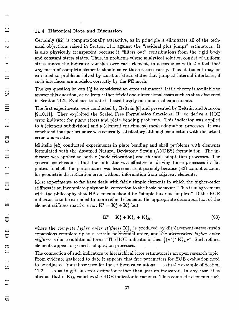
L
W
L--
v
W
±
r _
= =
11.4 Historical Note and Discussion
Certainly (82) is computationally attractive, as in principle it eliminates all of the tech-
nical objections raised in Section 11.1 against the "residual plus jumps" estimators. It
is also physically transparent because it "filters out" contributions from the rigid body
and constant stress states. Thus, in problems whose analytical solution consist of uniform
stress states the indicator vanishes over each element, in accordance with the fact that
any mesh of complete elements should solve those cases exactly. This statement may be
extended to problems solved by constant stress states that jump at internal interfaces, if
such interfaces are modeled correctly by the FE mesh.
The key question is: can U_, be considered an error estimator? Little theory is available to
answer this question, aside from rather trivial one-dimensional cases such as that discussed
in Section 11.2. Evidence to date is based largely on numerical experiments.
The first experiments were conducted by BeitrKn [8]:and presented by Beltr£n and Alarc6n
[9,10,11]. They exploited the Scaled Free Formulation functional 1-Ix to derive a HOE
error indicator for plane stress and plate bending problems. This indicator was applied
to h (element subdivision) and p (element enrichment) mesh adaptation processes. It was
concluded that performance was generally satisfactory although connection with the actual
error was erratic.
Militello [42] conducted experiments in plate bending and shell problems with elements
formulated with the Assumed Natural Deviatoric Strain (ANDES) formulation. The in-
dicator was applied to both r (node relocation) and rh mesh adaptation processes. The
general conclusion is that the indicator was effective in driving those processes in flat
plates. In shells the performance was less consistent possibly because (82) cannot account
for geometric discretization error without information from adjacent elements.
Most experiments so far have dealt with fairly simple elements in which the higher-order
stiffness is an incomplete-polynomial correction to the basic behavior. This is in agreement
with the philosophy that HP elements should be "simple but not simplex." If the HOE
indicator is to be extended to more refined elements, the appropriate decomposition of the
element stiffness matrix is not K _ = K_ + K_ but
K _ = K_ + K_,_ + K_,h, (83)
where the complete higher order stiffness K_c is produced by displacement-stress-strain
expansions complete up to a certain polynomial order, and the hierarchical higher order
stiffness is due to additional terms. The HOE indicator is then ½(ve)TK_h v'. Such refined
elements appear in p mesh-adaptation processes.
The connection of such indicators to hierarchical error estimators is an open research topic.
From evidence gathered to date it appears that free parameters for HOE evaluation need
to be adjusted from those used for the stiffness calculations -- as in the example of Section
11.2 -- so as to ge't an error estimator rather than just an indicator. In any case, it is
obvious that if Khh vanishes the HOE indicator is vacuous. Thus complete elements such
37

u
as the Linear Strain Triangle or Quadratic Strain Triangle [17] should be viewed as useless
for this purpose.
12. APPLICATION 3: FINITE ELEMENT TEMPLATES
The following stiffness matrix decomposition has been observed to recur in several FF and
ANDES elements (in particular, those mentioned in Section 10):
K - Kb +Hh = cLE LT +flwTswh, (84)
where c is the inverse of the element volume, area or length, f_ is a positive scaling factor,
L and Th are geometric matrices, E is the matrix of elastic moduli, and S depends on the
geometry and c0nstitutlve behavior as well as variational principle parametrization. (The
element index e has again been omitted from (84) for simplicity.)
Additional properties are as follows. The geometric matrix L, which is called the force-
lumping matrix in accordance with the FF terminology [12]' is responsible for satisfaction
of the patch test as well as that of element mixability properties; a detailed discussion of
these points has been recently given by Militello and Felippa [44]. The geometric matrix Th
annihilates the rigid-body modes and constant strain states. Together with S it provides
the correct rank to Ka, and thus is responsible for stability and accuracy.
Both L and S may contain free parameters. Any free parameters in L, however, must
be the same for all elements in an assembly; otherwise convergence and mixability are
impaired. On the other hand, parameters in S, as well as _, may vary from element to
element as long as the correct rank is preserved.
The form (84) will be called a finite element template, or template for short. The template
conjecture asserts that (84) is the most general form for all convergent FE of given degree-
of-freedom configuration.
A paxametrized expression that provides all such elements is called an universal template. A
parametrized expression that provides a practically important subset of all such elements is
called a generic template. Equations (69) and (70) provide examples of universal templates
for the 3-node bar and 2-node plane beam element, respectively.
Verification of this conjecture for more general elements would have the following projected
implications:
1. The confusion associated with the enormous number of "named" elements claimed in
the literature clears up: such elements, just like the canonical functionals discussed
previously, become points in a parametric continuum. Among other benefits, such
unification should help to streamline teaching of finite element theory and hence release
instruction time to cover problem modeling aspects.
2. Construction and testing of parametrized FE libraries can be greatly simplified.
3. Another realm of mesh adaptivity opens up: c adaptation, in which programs can
pick up elements from the paxaxnetrized continuum to strive for maximum accuracy
on a fixed mesh.
38
J
I
I
J
Q
i
I
U
I
==
g
I
m
=_
_I
I
J
w
=
_*K2_
"-W
w
. Several persistent mysteries may be cleared once and for all: convergence, mixability,
accuracy, locking, spurious modes, and distortion sensitivity. These properties could
be traced to components of the template (84) and interpreted physically.
13. CONCLUSION
The paper has surveyed the development of Parametrized Variational Principles and se-
lected applications to the Finite Element Method. It is shown that multifield PVPs provide
a framework by which classical variational principles may be embedded into a parametriz-
able continuum of functionals.
Three FEM applications have been reviewed: construction of high performance finite el-
ements, local error estimation, and element templates. These are in different stages of
development. While the application to HPFEs has succeeded beyond initial expectations,
the development of element-level error-eStimation has primarily relied on numerical exper-
iments, and the notion of templates is largely a conjecture suggested by isolated examples.
In the author's view, the following areas of variational methods merit further development:
• Parametrization of boundary terms, and use of such functionals in interfacing finite
element and variational Boundary Element discretizations (or, more generally, Trefftz
methods).
• Extension to dynamic and nonlinear problems. It is well known that finite elements
optimized for linear static analysis may not perform as well when time-dependency
and nonlinear effects are included. Functional parametrization opens up possibilities
of extending the aforementioned FEM applications to such cases.
following FEM-application areas would benefit from focused research work:
Establishment of a general convergence theory of FEM based on PVPs. Areas that
require special attention are: dependence of element performance on choice of param-
eters, mixability properties, and limitation principles.
• Development of a sound a-po,teriori error estimation methodology for two- and three-
dimensional nonconforming elementsi in particular establishing connections between
HOE and hierarchical error estimators.
. Verification or disproval of the template conjecture. If proven, proceed to exploit the
benefits outlined in Section 12.
The
Acknowledgements
The author is indebted to Professor Bernard Nayroles for the invitation to address the 1992 SIMG.
The preparation of this work has been supported by NASA Langley Research Center under GrantNAS1-756, monitored by Dr. J. Housner.
39

I
.
.
References
1. D.J. Allman, A compatible triangular element including vertex rotations for plane elasticity
analysis, Computers eJ Structures, 19 (1984) 1"8
2. K. Alvin, H. M. de la Fuente, B. Haugen and C. A. Felippa, Membrane elements with corner
drilling freedoms: I. The EFF element, Finite Elements in Analysis and Design, 12, (1992),163-187
J. H. Argyris and S. K elsey, Energy _Theorems and Structural Analysis, Butterworths Sci.
Pubs., London (1960); reprinted from Aircraft Engrg. 26 (1954) and 27 (1955)
4. I. Babu_ka, The selfadaptive approach in the finite element method, in The Mathematics
of Finite Elements and Applications H MAFELAP 75, ed. by J. R. Whiteman, Academic
Press, London (1975) I25Li42. : ....... _...... _
I. Babu_ka and A. Miller, A feedback finite element method with a-posteriori error estimation:
Part I. The finite element method and some basic properties of the a-posteriori error indicator,
Comput. Methods Appl. Mech. Engrg., 61 (1987) 1±40
6. I. Babu_ka, R. Dur£n and R. Rodriguez, Analysis of the efficiency of an a-posteriori error
estimator for linear triangular finite elements, SIAM J. Numer. Anal., 29 (1992) 947-964
7. K.J. Bathe and E. N. Dvorkin, A four-node plate bending element based on Mindlin/Reissner
plate theory and a mixed interpolation, Int. J. Numer. Meth. Engrg., 21 (1985) 367-383
8. F.J. Beltr£n, Estimadores de error basados en principios variacionales multicampo para
c61culos pot elementos rialtos, Tests Doctoral, Universidad Polit_cnica de Madrid (1990)
9. F.J. Beltr£n and E. Alarc6n, Estimadores del error de discretizaci6n con principios varia-
cionales multicampo: I. Elasticidad, Rev. Internat. M_todos Numer. Cdlculo y Diserio en
Ingenieria, 8 (1992) 43-55
10. F.J. Beltr£n and E. Alarcdn, Estimadores del error de discretizaci'on con principios varia-
cionales multicampo: II. Flexi6n de placas, Rev. Internat. M_todos Numer. Cdlculo y Dise,_o
en Ingenieria, 8 (1992) 139-156
11. F.J. Beltr£n and E. Alarc6n, Accuracy estimates based on multifield variational principles,
Eur. J. Mech. A//Solids, 11 (1992) 487-518
12. P.G. Bergan and M. K. Nyg£rd, Finite elements with increased freedom in choosing shape
functions, Internat. J. of Numerical Methods in Engineering, 20 (1984) 643-664
13. P.G. Bergan and C. A. Felippa, A triangular membrane element with rotational degrees of
freedom, Comput. Methods Appl. Mech. Engrg., 50 (1985) 25-69
14. R.W. Clough, The finite element method in plane stress analysis, J. Struct. Div. ASCE,
Proc. 2nd Conf. Electronic Computation (1961) 345-378
15. R. Courant, Variational methods for the solution of problems of equilibrium and vibrations,
Bull. Amer. Math. Soc., 49 (1943) 1-23
16. L. Demkowicz, J. T. Oden, W. Rachowicz and O. Hardy, Towards a universal h-p adaptive
finite element Strategy, Part 1. Constrained approximation and data structure, Comput.
Methods Appl. Mech. Engrg., 77 (1989) 79-112
17. C.A. Felippa, Refined finite element analysis of linear and nonlinear two-dimensional struc-
tures, Ph. D. Dissertation, Department of Civil Engineering, University of California at
Berkeley, Berkeley, CA (1966)
4O
J
g
Im
i
II
m
I
II
Z
ZII
m_
J
u
J

= ,
w
[ ]
w
u
L JE
= =
18. C.A. Felippa and P. G. Bergan, A triangular plate bending element based on an energy-
orthogonal free formulation, Comput. Methods Appl. Mech. Engrg. , 61 (1987) 129-160
19. C.A. Fellppa, Parametrized multlfield variational prineipies in elasticity: I. Mixed function-
als, Commun. Appt. Numer. Methods, 5 (1989) 69-78
20. C.A. Felippa, Parametrized multifield variationalprinciples in elasticity: II. Hybrid func-
tionals and the free formulation, Commun. Appl. Numer. Methods, 5 (1989) 79-88
21. C.A. Felippa, The extended free formulation of finite elements in linear elasticity, J. Appl.
Mech., 56 (1989) 609-616
22. C.A. Felippa and C. Militello, Developments in variational methods for high performance
plate and shell elements, in Analytical and Computational Models for Shells, CED Vol. 3,
ed. by A. K. Noor, T. Belytschko and J. C. Simo, The American Society of MechanicalEngineers, ASME, New York (1989) 191'216
23. C.A. Fellppa and C. Militello, Variational Formulation of High Performance Finite Elements:
Parametrized Variational Principles, Computers gY Structures, 36 (i990) 1-11
24. C.A. Felippa, Parametrized variational principles encompassing compressible and incom-
pressible elasticity, Internat. Y. Solids Structures, 29 (1991) 57-68
25. C.A. Felippa, Parametrized variational principles for micropolar elasticity, Internat. J. Solids
Structures, 29 (1992) 2709-2721
26. C.A. Felippa and C. Milltello, Membrane elements with corner drilling freedoms: II. The
ANDES element, Finite Elements in Analysis and Design, 12 (1992) 189-201
27. C. A. Felippa and Alexander, S., Membrane elements with corner drilling freedoms: III.Implementation and performance validation, Finite Elements in Analysis and Design, 12
(1992) 203-239
28. C.A. Felippa and J. Schuler, Parametrized variational principles for electromagnetodynamics,
Proceeding ASME/ASCE Conference Charlottesville, VA June 1993, to appear in boundASME volume
29. R.A. Frazer, W. J. Duncan and A. R. Collar, Elementary Matrices, Cambridge Univ. Press,
(1963) (First edition 1938)
30. C. Fox, An Introduction to the Calculus of Variations, Dover, New York (1950)
31. F. Hartmann, The Mathematical Basis of Structural Mechanics, Springer-Verlag, Berlin, 1985
32. H. C. Huang and E. Hinton, A new nine node degenerated shell element with enhanced
membrane and shear interpolation, Int. J. Numer. Meth. Engrg., 22 (1986) 73-92
33. T.J.R. Hughes and F. Brezzi, On drilling degrees of freedom, Comput. Methods Appl. Mech.
Engrg., 72 (1989) 105-121
34. B. Langefors, Analysis of elastic structures by matrix coefficients, with special regard to
semimonocoque structures, J. Aero. Sci., 19 (1952) 451-458
35. S. Levy, Computation of influence coefficients for aircraft structures with discontinuities and
sweepback, J. Aero. Sei., 14, (1947) 547-560
36. S. Levy, Structural analysis and influence coefficients for delta wings, J. Aero. Sci., 20,
(1953) 677-684
37. S. Liu and Z. Jiang, General form of the generalized variational principle in elasticity, Corn-
muM. Appl. Numer. Methods, 5 (1988) 749-760
41

38. S.Liu, ExtendedGurtin's variationalprinciplesfor linearelastodynamics,in Computational
Mechanics '91, ed. by S. N. Atluri, D. E. Beskos, R. Jones and G. Yagawa, ICES Publications,
Atlanta, GA (1991) 649-650
39. R.J. Melosh and P. V. Marcal, An energy basis for mesh refinement of structural continua,
Internat. J. Numer. Methods Engrg., 11 (1977) 1083-1091.
40. C. Militello and C. A. Felippa, A variational justification of the assumed natural strain
formulation of finite elements: I. Variational principles, Computers eJ Structures, 34 (1990)
431-438
41. C. Militello and C. A. Felippa, A variational justification of the assumed natural strainformulation of finite elements: II. The four-node C O plate element, Computers eJ Structures,
84 (1990) 439-444
42. C. Militell0, Application of Parametrized Variational Principles to the Finite Element
Method, Ph. D. Dissertation, Department of Aerospace Engineering Sciences, University of
Colorado, Boulder, CO (1991)
43. C. Militello and C. A. Felippa, The first ANDES elements: 9-dof plate bending triangles,
Comput. Methods Appl. Mech. Engrg., 93 (1991) 217-246.
44. C. Militello and C. A. Felippa, The individual element test revisited, in The Finite Element
Method in the I990s, ed. by E. Ofiate, J. Periaux and A. Samuelsson, Springer-Verlag, Berlin
(1991) 554-564
45. C. Militell0 and C. A. Felippa, r-adaptive methods based on element level error estimators
for parallel analysis of plates and shells, presented to First US National Congress on Compu-
tational Mechanics, Chicago (July 1991); also in 33rd AIAA/ASCE/ASME/AIH Structures,
Structural Dynamics and Materials Conference Proceedings, Dallas (April 1992)
46. J.T. Oden and J. N. Reddy, On dual complementary variational principles in mathematical
physics, Int. J. Engrg. Sci., 12 (1974) 1-29
47. J.T. Oden and J. N. Reddy, Variational Methods in Theoretical Mechanics, Springer-Verlag
(1982)
48. J.T. Oden and L. Demkowicz, Advances in adaptive improvements: A survey of adaptive
methods in computational mechanics, in State of the Art Surveys in Computational Mechan-
ics, ed. by A. K. Noor and J. T. Oden, ASME, New York (1988) 441-468
49. J.T. Oden, L. Demkowicz, W. Rachowicz and T. A. Westermann, Towards a universal h-p
adaptive finite element strategy, Part 2. A posteriory error adaptation, Comput. Methods
Appl. Mech. Engrg., 77 (1989) 113-180
50. K. C. Park and G. M. Stanley, A curved C O shell element based on assumed natural-
coordinate strains, J. Appl. Mech., 53 (1976) 278-290
51. T. H. H. Plan and P. Tong, Basis of finite element methods for solid continua, Internat. J.
Numer. Methods Engrg., 1 (1969) 3-28
52. T. H. H. Plan, Finite element methods by variational principles with relaxed continuity
requirements, in Variational Methods in Engineering, Vol. 1, ed. by C. A. Brebbia and H.Tottenham, Southampton University Press, Southhampton (1973)
53. J.N. Reddy, On complemnentary variational principles for the linear theory of plates, Journal
of Structural Mechanics, 4 (1976) 417-436
54. J.N. Reddy, Energy and Variational Methods in Applied Mechanics, Wiley/Interscience, New
York, 1984
42
l
J
I
g
m
g
II!
I
W
U
u
W
mm
g
zm
im

W
W
k_
55. R. Santilli, Foundations of Theoretical Mechanics I, Springer-Verlag, Berlin (1978)
56. G. Sewell, An adaptive computer program for the solution of Div(P(X,Y)GradU) =
F(X,Y, U) on a polynomial region, in The Mathematics of Finite Elements and Applica-tions H MAFELAP 75, ed. by J. R. Whiteman, Academic Press, London (1975) 543-554.
57. M.J. Sewell, Mazimum and Minimum Principles, Cambridge, (1987)
58. J.C. Simo and T. J. R. Hughes, On the variational foundations of assumed strain methods,
J. Appl. Mech., 53 (1986) 51-54
59. E. Tonti, On the mathematical structure of a large class of physical theories, Accad. Naz. dei
Lincei, Series III, 52 (1972) 48-56
60. E. Tonti, A mathematical model for physical theories, Accad. Naz. dei Lincei, Series VIII,
52 (1972) 175-181,350-356
61. M.J. Turner, R. W. Clough, 1:[. C. Martin and L. J. Topp, Stiffness and deflection analysis
of complex structures, J. Aero. Sci., 23 (1956) 805-823
62. B.D. Vujanovic and S. E. Jones, Variational Methods in Nonconsewative Phenomena, Aca-
demic Press (1989)
63. K. Washizu, Variational Methods in Elasticity and Plasticity, Pergamon Press (1972)
64. O.C. Zienkiewicz, D. W. Kelly, J. P. Gago, J. P. and I. Babu_ka, Hierarchical finite element
approaches, error estimates and adaptive refinement, in The Mathematics of Finite Elements
and Applications IV (MAFELAP VI), ed. by J.R. Whiteman, Academic Press, New York
(1981)
65. O.C. Zienkiewicz and A. Craig, A-posteriori error estimates and adaptive mesh refinement in
the finite element method concepts, Chapter 5 in The Mathematical Basis of Finite ElementMethods, ed. by D. Griffiths, Clarendon Press, Oxford (1984)
66. O.C. Zienkiewicz and A. Craig, Adaptive refinement, error estimates, multigrid solution and
hierarchic finite element method concepts, Chapter 2 in Accuracy Estimates and Adaptive
Refinements in Finite Element Computations, ed. by I. Babu_ka et.al., John Wiley and Sons,
Chichester (1986) .......
67. O.C. Zienkiewicz and J. Z. Zhu, A simple error estimator and adaptive procedure for practical
engineering analysis, Internat. J. Numer. Methods Engrg., 24 (1987) 337-357.
: ! _<r£. !
L_
w
z=
43

COMPUTER METHODS IN APPLIED MECHANICS AND ENGINEERING -"
Editors:
John. H. Argyris
Thomas J.R. Hughes
J. Tinsley Oden
InstRute for Computer Applications, -- L_lit, rmi Qlt-i_.e --,
Pfaffenwaldring 27, W-7000 Stuttgart 80, German); Tel. No.." (0711) 685-3593
Imperial College of Science and Technb-log_v, Prince Consort l_d., London ==SW7, = United Kingdom
Stanford University, Division of Applied Mechanics, Durand Building, Stanford, California 94305-4040,
USA, Tel. No- (415) 723-2040, Fax No.." (415) 723-1778
TICOM Office, 3500 West Balcones Center Drive, Austin,
Texas 78759, USA, Tel. No.: (512) 471-3312, Fax No.: (512) 471-8694
l[I
D
J
I
April 5, 1993II
Dr. Carlos Felippa ...............University of ColoradoDepartment of Aerospace Engineering and
Center for Space Structures and ControlsBoulder, CO 80309 =
Dear Carlos:
Ref: #404 "Parametrized Variational Principles and Applications To ComputationalMechanics"
by C__lo_s_Felippa
We have now obtained a review on your paper, "Parametrized Variational Principles andApplications To Computational Mechanics". The review_ers state that this is an excellentpaper, although it requires a few minor revisions. Please look over the enclosedcomments and, if you wish, submit a revised version of the paper for a quick final review.
Thank you for allowing Computer Methods in Applied Mechanics and Engineering toconsider your work, and we look forward to hearing from you.
Sincerely,
Editor
JTOIIc
Enclosure
zm
I
I
mg
U
B
J
g
Journal published by." Elsevier Science Publishers BN. (North-Holland), P.O. Box 1991, 1000 BZ Amsterdam, The Netherlands Iw
Top Related