


Languages
Pages
Legal


abbr
1

Time to Produce and Emerging Market Crises ∗
Felipe Schwartzman
January 19, 2010
Abstract
This paper argues that interest rates affect output through their impact on the cost of variable
inputs such as materials and labor. This effect occurs because of time lags in the production process.
To test the theory, I exploit the following cross-sectional implication: industries that usually hold more
inventories relative to their variable costs should react more strongly to changes in the cost of capital.
I find that during emerging market crises there is a large and robust reallocation towards sectors
with low inventory-to-cost ratios. I set up a multi-sector general equilibrium model with production
lags which match the inventory-to-cost ratios in the data. Exogenous shocks calibrated to reproduce
movements in aggregate variables during the crises generate a sectoral reallocation compatible with
the empirical predictions. Furthermore, the model generates a sizeable and quick reaction of aggregate
output in reaction to an isolated interest rate shock, which is consistent with findings in the previous
literature. All these results rely only on the assumption about the production technology, without
any reference to financial or payment frictions.
∗I would like to thank Nobu Kiyotaki and Markus Brunnermeier for advising me in this work. I also thank GeorgeAlessandria, Tiago Berriel, Carlos Carvalho, Bo Honore, Oleg Itskhoki, Ryo Jinnai, Pat Kehoe, Kalina Manova, VirgiliuMidrigan, Fernanda Nechio, Esteban Rossi-Hansberg, Huntley Schaller, Sam Schulhofer-Wohl, Hyun Shin, Chris Sims, MarkWatson, Adam Zawadowski and participants in various workshops and seminars in Princeton for helpful advice. All remainingerrors and omissions are of my entire responsibility.

1 Introduction
This paper argues that interest rates affect output through their impact on the cost of variable inputs
such as materials and labor. The cost of variable inputs increases in the interest rate because of time
lags in the production process. When a firm sets out to produce a good, first it has to acquire raw
materials and put workers to work, and only after a period of time it is able to sell the finished good.
In the interim, the firm foregoes interest income or incurs interest costs. If the interest rate goes up,
the production process becomes more costly so that the firm optimally chooses to reduce its sales.
I exploit the following cross-sectional implication of the theory: industries that usually hold more
inventories relative to their variable costs should react more strongly to changes in the cost of capital.1
The reason is that inventories account for the value of all variable inputs accumulated between the time
of their acquisition and the sale of the corresponding output. As a consequence, the ratio between total
inventories and variable costs captures the importance of the foregone interest rate income associated
with the purchase of variable inputs.2
The empirical analysis focuses on episodes in which the link between capital flows and output
was most likely to be visible. These are the sudden stop episodes identified by Calvoetal:2006b. The
discrete jump in current account surplus observed in these episodes suggest that they were largely
unforeseen shocks. The large and persistent drop in investment/output ratio that follows suggests a
large and persistent increase in the cost of capital. Together these suggest that these episodes provide
interesting natural experiments on the effects of shocks to the cost of capital on output.
I find that in the course of these episodes there is a large and robust reallocation towards sectors
with low inventory-to-cost ratios. Figure ?? shows the reallocation pattern in the data. Each point
refers to a manufacturing industry. The vertical axis depicts the difference in the log of value added
in the year when GDP was at its lowest and the value three years before, averaged over 21 sudden
stop episodes.3 The horizontal axis represents a proxy for the inventory-to-cost ratio calculated for
each industry.4 As I discuss in section ??, the addition of controls reduces the slope of the regression
coefficient, but the correlation is remarkably robust.
The reduced form estimates establish that the reallocation goes in the direction predicted by
the theory. To assess whether time lags in production can plausibly account for the magnitude of
the estimated effects, I set up a multi-sector general equilibrium model with delays between the
1The bulk of inventories are raw materials and work-in-process, the value of which are naturally tied to production plans.Also, finished goods inventories have been found to follow sales quite closely at yearly frequencies, so that it is adequate tointerpret these as factors of production [?].
2As opposed to inventory to sale ratio, since sales also include markups and income of fixed factors which have little rolein the short term decisions.
3I use volume indices for value added4I use data from manufacturing industries in the US, following the tradition initiated by Rajanzingales:1998. Total
inventories are the sum of the stocks of raw materials, work in process and finished good inventories, and the variable costsinclude materials and direct labor costs. Inventories are measured in dollars and costs are measured in dollars per month.Hence the ratio is measured in months. A ratio of 2 implies that firms hold an amount of inventories equivalent to twomonths worth of costs.
3
use of inputs and the completion of the output. I calibrate the production lags so that they are
compatible with the inventory-to-cost ratios in the data. I then simulate a crisis in the model as
a combination of shocks to foreign interest rate and total factor productivity, chosen to match the
magnitude and persistence of changes in GDP and fixed investment. The model is able to generate a
sectoral reallocation in response to a crisis-like event in line with the estimates from the data.
Lastly, I can also use the model to assess the importance of the production time channel for the
impact of interest rate shocks on aggregate output. The model implies that the shock to the foreign
interest rate accounts for about one quarter of the initial drop in output. In particular, because of
the interest rate shock alone, GDP drops about 4% over the first two quarters after the shocks.
This large effect may come across as puzzling given the short lags in the production process. The
main reason is a relatively high level of “substitution”, in the sense emphasized by KingRebelo:1999.
I allow firms to choose capacity utilization and, following the practice in the Small Open Economy
RBC literature, do not allow for wealth effects in labor supply. These assumptions imply that the
supply fixed capital and labor do not impose important constraints on the effect of the shocks.
The notion that interest rates affects the cost of variable inputs is hardly new. However, the
usual mechanisms rely on some form or another of payment frictions. For example, christianoeichen-
baum:1992 propose that firms need to hold cash in order to pay the wage bill, so that if the interest
rate goes up, these payments become more costly. This assumption is problematic when it comes
to emerging market economies that underwent periods of very large inflation. The reason is that,
with a cash-in-advance constraint, the financial cost is increasing not in the real, but in the nominal
interest rates. During inflationary times the variability in inflation, and hence in the nominal interest
rate, was larger by an order of magnitude when compared with the post-stabilization period. Given a
cash-in-advance constraint, this would imply a commensurate difference in the volatility of production
costs and of output.5
NeumeyerPerri:2004 propose that in emerging markets payments are made in real, non-interest
rate bearing assets instead of cash. This assumption allows them to match the negative correlation
between detrended output and the real interest rate on government bonds observed in Argentina, while
encompassing both periods with high and low inflation. Their success has prompted many authors
to use a similar device in more elaborate models of emerging market business cycles.6 While the
assumption is successful in terms of its aggregate implications, Charikehoemagrattan:2005 criticize it
for the lack of an empirical counterpart. This paper resolves the issue by proposing that the purchase
of variable inputs is itself a real, short-term investment, so that no recourse to payment frictions is
needed.
This paper discusses how a change in the cost of capital affects output, but it leaves open the
5Nevertheless, cash-in-advance constraints in the payment of inputs has a long tradition in the emerging market businesscycle literature, for example Cavallo:1981. See AgenorMontiel:2002, Ch. 6 and 7 for a discussion of this early literature.
6See for example christianogustroldos:2004, Mendoza:2006, UribeYue:2006, Otsu:2007 and MendozaYue:2008. An excep-tion is GertlerGilchristNatalucci:2007, in that interest rate shocks affect production quickly through the impact of changesin the real exchange rate on capacity utilization decisions.
4

determination of this cost. This task is undertaken, for example, by Mendoza:2006. The author
demonstrates how a business cycle model with occasionally binding credit constraint at the level of
the economy is able to generate alternating periods of normal business cycle variations and sudden
stops.7 In itself, however, these frictions do not imply a drop in output, and Mendoza recurs to
a payment-in-advance constraint to get this effect. On the empirical side, a similar point can be
made about the studies by Kroszneretal:2006 and Dellariccia:2007. They find that, in banking crises,
industries that rely more on external finance to fund long term investment lose relatively more of their
output. Their empirical results illuminate the effect of banking crises on the cost of capital, but they
leave open how this exposure translates into a drop in output.
The empirical findings in this paper are complemented by independent work by TongWei:2009.
Using data from emerging market firms, the authors show that a high inventory-to-sale ratio was
associated with a relatively large drop in share-prices in the aftermath of the latest global crisis. Their
price evidence complements the quantity evidence presented here. Raddatz:2006 presents another set
of related empirical findings. He finds that industries with high inventory-to-sale ratio are relatively
more volatile in countries with a low level of financial development. His findings emphasize the role
of the financial system in providing liquidity insurance.8
The paper proceeds as follows: Section 2 uses a simple partial equilibrium example to lay out the
link between theory and data. In particular, it shows that if production time is allowed for then
firms which normally hold a higher inventory-to-cost ratio will respond more strongly to interest rate
shocks. Section 3 contains the data analysis. It documents the cross-industry correlation between
the inventory-to-cost ratio and the change in value added during emerging market crises, providing
various robustness checks. Section 4 introduces the general equilibrium business cycle model, discusses
its calibration, and reports the results of the different experiments. Section 5 concludes the paper.
2 Time to produce in Partial Equilibrium
This section discusses, in a partial equilibrium setup, the key cross-sectional prediction of the time to
produce model: shocks to the interest rate have an impact on sales that is largest for firms that have
a large steady state inventory-to-cost ratio.
I construct the argument in two steps. First, I introduce the production function that underlies
the analysis and show that, after a short transition period, the impact of a persistent interest rate
shock on sales is increasing in the share of inputs that a firm has to acquire early on.9
7Like here, the marginal cost of capital in Mendoza:2006 is the same for all firms. Implicitly, the balance sheet constraintsin his model are the ones faced by domestic financial intermediaries as opposed to domestic productive units, as suggestedby Krishnamurthy:2003.
8Markups vary less than inventories across firms, so that inventories to cost and inventories to sale ratios are normallyclosely linked.
9In the exposition below I focus on sales as a measure of economic activity, since these are more conceptually straightfor-ward than value added. I discuss how the results change economic activity is measured using value added instead.
5

Second, I show that this share can be mapped into the ratio between inventories and variable costs.
This is the key insight that drives the paper. This mapping underlies the empirical analysis in section
3 and the calibration in section 4.
2.1 A one time shock to the interest rate
The production function is an application of Kydlandprescott:1982 time to build technology. I use
the term “time to produce” instead of “time to build” to emphasize the rather short-horizon process
of transforming variable inputs into manufactured goods, as opposed to the more time consuming
process of building ships or factories. I take a broad view of production that includes the storage
of inputs and finished goods in order to economize on logistics and avoid stock-outs. This is akin to
Ramey:1989 suggestion that inventories can be usefully modeled as factors of production.10
In order to sell output at t, a firm must acquire inputs in t− 1 and t− 2. The production function
is Cobb-Douglas with decreasing returns to scale, as follows:11
Yt =([Zt (0)]1−ω [Zt−1 (1)]ω
)φ, φ < 1
Where Zt (v) is a composite of inputs acquired in t to generate a sale v periods ahead.
Consider the perfect foresight path of sales after a one time, unexpected shock to the interest
rate. Suppose firms are in steady state and at t = 0 they find that the future path of interest rate
will change. The new interest rate path is a perturbation around the old steady state that decays
geometrically, at a rate η. By assumption, the prices of output and inputs do not change. As a
consequence, this is a partial equilibrium exercise.
I assume that Zt (v) is a composite of the same set of goods irrespective of v, the horizon to which
it is assigned. This implies that I can denote a price index for Zt (v) which is independent of v. The
problem of the firm at t = 0 is:
maxZt(v),Yt
∞∑t=0
t∏s=0
1Rs
[ptYt − qtZt (0)− qtZt (1)]
s.t. : Yt =([Zt (0)]1−ω [Zt−1 (1)]ω
)φZ−1 (1) = z
Where qt and pt are, respectively, a price index for the composite of inputs and the price of the
final goods, and Rt is the interest rate between periods t and t+ 1. The constraint implies that input
10However, the production function approximates the treatment in MacciniMooreSchaller:2004 more closely in that itemphasizes the role of flows of goods into production, rather than stocks
11The decreasing returns to scale may stem from fixed inputs. This is a minor omission since the share of variable inputsin manufacturing production is typically above 80%. In the calibrated model I allow for constant returns to scale at the firmlevel.
6

choices made before t = 0 cannot be changed.
I can rewrite the problem as a sequence of maximization problems:
t=0:
maxZ0(1),Y0
p0Y0 − q0Z0 (0)
s.t. : Y0 =(Z0 (0)1−ω zω
)φ
The cost of inputs acquired at t = −1 is sunk, but not the ones acquired in t = 0. The profit
maximizing output is:
Y0 = χ0zωφ
(q0p0
)− (1−ω)φ1−(1−ω)φ
Where χ0 is a constant term. Note that output is insensitive to the interest rate. This is because
all inter-temporal decisions relevant for period t production were made beforehand.
t≥ 1:
From t ≥ 1 onward, the problem of the firm is:
maxZt(v),Yt
ptYt − qtZt (0)−Rt−1qt−1Zt−1 (1)
s.t. : Yt =([Zt (0)]1−ω [Zt−1 (1)]ω
)φ
Now, the profit maximizing output is
Yt = χ
[(Rt−1qt−1)
ω (qt)1−ω
pt
]− φ1−φ
Where again χ is a constant term. This implies that
dYtYt
= − φ
1− φωdRt−1
Rt−1
Since dRtRt
= η dRt−1
Rt−1, I can write the relationship between current output and current interest rate
as:
7
dYtYt
= − φ
1− φ
ω
η
dRtRt
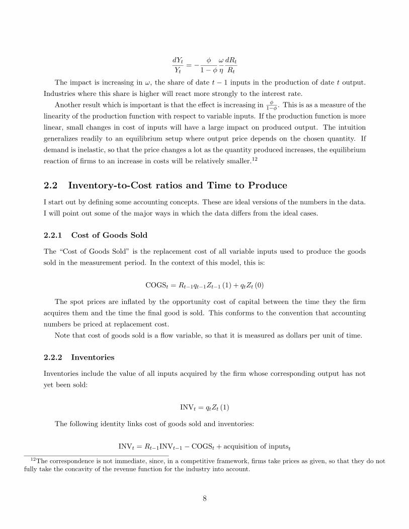
The impact is increasing in ω, the share of date t − 1 inputs in the production of date t output.
Industries where this share is higher will react more strongly to the interest rate.
Another result which is important is that the effect is increasing in φ1−φ . This is as a measure of the
linearity of the production function with respect to variable inputs. If the production function is more
linear, small changes in cost of inputs will have a large impact on produced output. The intuition
generalizes readily to an equilibrium setup where output price depends on the chosen quantity. If
demand is inelastic, so that the price changes a lot as the quantity produced increases, the equilibrium
reaction of firms to an increase in costs will be relatively smaller.12
2.2 Inventory-to-Cost ratios and Time to Produce
I start out by defining some accounting concepts. These are ideal versions of the numbers in the data.
I will point out some of the major ways in which the data differs from the ideal cases.
2.2.1 Cost of Goods Sold
The “Cost of Goods Sold” is the replacement cost of all variable inputs used to produce the goods
sold in the measurement period. In the context of this model, this is:
COGSt = Rt−1qt−1Zt−1 (1) + qtZt (0)
The spot prices are inflated by the opportunity cost of capital between the time they the firm
acquires them and the time the final good is sold. This conforms to the convention that accounting
numbers be priced at replacement cost.
Note that cost of goods sold is a flow variable, so that it is measured as dollars per unit of time.
2.2.2 Inventories
Inventories include the value of all inputs acquired by the firm whose corresponding output has not
yet been sold:
INVt = qtZt (1)
The following identity links cost of goods sold and inventories:
INVt = Rt−1INVt−1 − COGSt + acquisition of inputst12The correspondence is not immediate, since, in a competitive framework, firms take prices as given, so that they do not
fully take the concavity of the revenue function for the industry into account.
8

Where previous period inventories are inflated by the interest rate so that they are valued at
replacement cost. While in practice the valuation of costs and inventories deviates from the ideal
represented above, the rest of accounting identity above is normally respected.13
2.2.3 Inventory-to-Cost Ratio
The inventory-to-cost ratio is:
INVt
COGSt=
qtZt (1)Rt−1qt−1Zt−1 (1) + qtZt (0)
Under perfect foresight, the Cobb-Douglas assumption implies that:
INVt
COGSt=ωφYt+1
φYt
This is a forward looking variable, since inventories reflect future production plans. It will fluctuate
with the business cycle as firms change their production plans. Note that since inventories are a stock
variable, measured in dollars, and the cost of goods sold is a flow variable, measured in dollars per
unit of time, the inventory-to-cost ratio is measured in units of time.
For the purposes of this paper, the interesting quantity is the steady state inventory-to-cost ratio,
that is, the one obtained when Yt = Yt−1 for all t. This satisfies:
INVCOGS
=qZ (1)
RqZ (1) + qZ (0)
Again, applying the Cobb-Douglas assumption:
INVCOGS
=ωφY
φY= ω
Recall that ω plays an important role in characterizing the impact of the interest rate shock on
sales. In particular, from t ≥ 1 onwards, the impact is increasing in ω. This implies that the impact
of an interest rate shock is, everything else constant, increasing in the inventory-to-cost ratio.
If the persistence parameter η is close to 1, then
dYtYt
∼=INV
COGSφ
1− φ
dRtRt
13In particular, accounting practices differ depending on whether inventories are valued at the cost of the inputs boughtmost recently (Last In First Out) or at the price of the oldest inputs who have not yet been deducted from inventories (FirstIn First Out) or still other practices
9

So that the impact of interest rate on output is directly proportional to the inventory-to-cost ratio.
This latter result generalizes to arbitrary convex production functions with inputs included many
periods in advance. The discussion of is in Appendix B.
2.2.4 Caveats
A few caveats are worth mentioning. First, inventory and costs rarely if ever account for financing
costs. This problem is not particularly important if the period of time considered is not very large. In
the data, inventory turnover ratios for the manufacturing sector are around 2 months. This implies
that the financing costs are fairly small.
Second many important costs may not be accounted for in the cost of goods sold and in inventories,
notably maintenance cost of capital and administrative labor. However, it is normally the case that
whatever costs are accounted for under “cost of goods sold”, they are also included in inventories,
including direct labor costs. This implies that the ratio is approximately correct if the omitted costs
have a time profile similar to the included ones.
Third, the actual measurements of productive activity are based on value added and not on sales.
Because value added data includes the change in inventories, it has a forward looking component.
This implies that the reaction of value added to interest rate shocks should be faster than the reaction
of sales. However, as the economy evolves along the perfect foresight path, the two measures become
tightly linked, as demonstrated in Appendix A.
3 Data Analysis
This section presents the empirical results. It shows that during emerging market crises there is a
strong reallocation towards sectors with lower inventory-to-cost ratio. The data analysis in this section
shows that the reallocation does not reflect other plausible explanations and is a robust feature of
emerging market crises, having occurred in the 80’s and the 90’s, in Latin America and in other
continents. Last, this section shows that the reallocation was persistent, so that it was not a mere
reflection of short run inventory adjustment dynamics.
3.1 Events
The analysis centers on events that Calvoetal:2006b identify as output collapses following Systemic
Sudden Stops.14 The list of episodes is in table ?? These are restricted to emerging market economies,
and consist of large output drops that occurred together with unusually large reversals in current
account. In order to isolate “systemic” episodes, the authors focus on periods when international
rates at which emerging market countries borrowed were relatively high. This filter helps assure that
the episodes were somehow linked to the difficult foreign financial environment. The dates picked
14See the above mentioned paper and Calvoetal:2004 for further details of how exactly these events were selected.
10
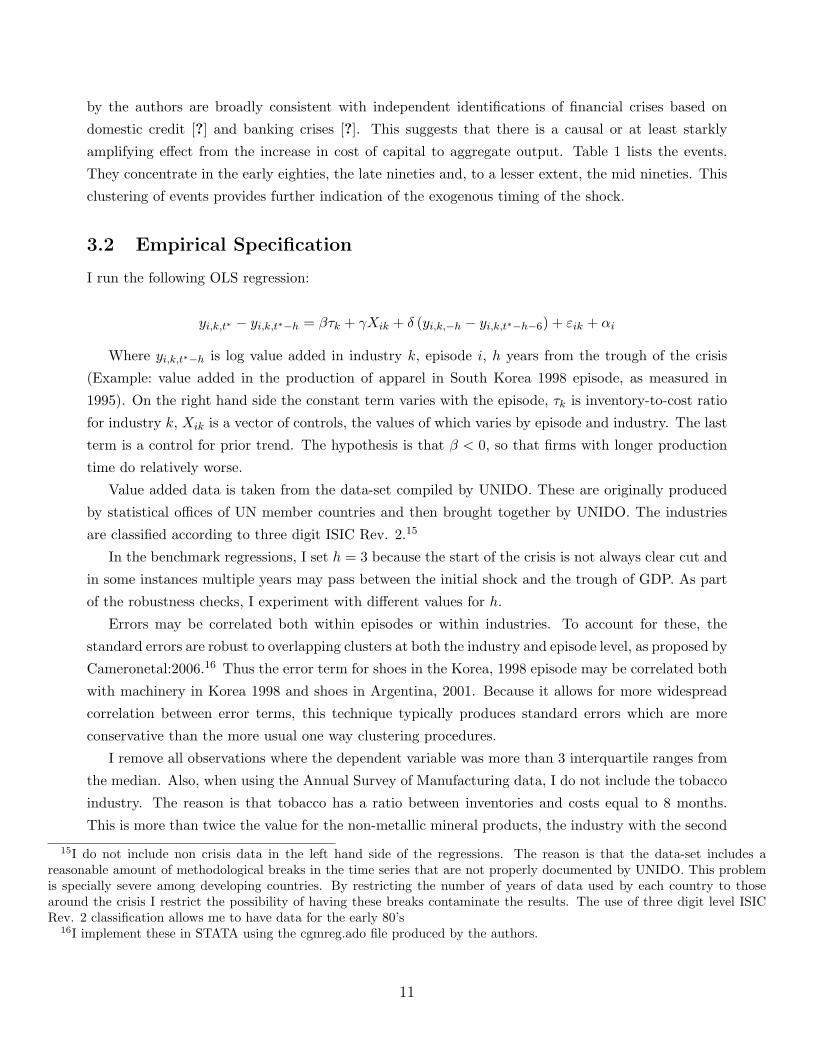
by the authors are broadly consistent with independent identifications of financial crises based on
domestic credit [?] and banking crises [?]. This suggests that there is a causal or at least starkly
amplifying effect from the increase in cost of capital to aggregate output. Table 1 lists the events.
They concentrate in the early eighties, the late nineties and, to a lesser extent, the mid nineties. This
clustering of events provides further indication of the exogenous timing of the shock.
3.2 Empirical Specification
I run the following OLS regression:
yi,k,t∗ − yi,k,t∗−h = βτk + γXik + δ (yi,k,−h − yi,k,t∗−h−6) + εik + αi
Where yi,k,t∗−h is log value added in industry k, episode i, h years from the trough of the crisis
(Example: value added in the production of apparel in South Korea 1998 episode, as measured in
1995). On the right hand side the constant term varies with the episode, τk is inventory-to-cost ratio
for industry k, Xik is a vector of controls, the values of which varies by episode and industry. The last
term is a control for prior trend. The hypothesis is that β < 0, so that firms with longer production
time do relatively worse.
Value added data is taken from the data-set compiled by UNIDO. These are originally produced
by statistical offices of UN member countries and then brought together by UNIDO. The industries
are classified according to three digit ISIC Rev. 2.15
In the benchmark regressions, I set h = 3 because the start of the crisis is not always clear cut and
in some instances multiple years may pass between the initial shock and the trough of GDP. As part
of the robustness checks, I experiment with different values for h.
Errors may be correlated both within episodes or within industries. To account for these, the
standard errors are robust to overlapping clusters at both the industry and episode level, as proposed by
Cameronetal:2006.16 Thus the error term for shoes in the Korea, 1998 episode may be correlated both
with machinery in Korea 1998 and shoes in Argentina, 2001. Because it allows for more widespread
correlation between error terms, this technique typically produces standard errors which are more
conservative than the more usual one way clustering procedures.
I remove all observations where the dependent variable was more than 3 interquartile ranges from
the median. Also, when using the Annual Survey of Manufacturing data, I do not include the tobacco
industry. The reason is that tobacco has a ratio between inventories and costs equal to 8 months.
This is more than twice the value for the non-metallic mineral products, the industry with the second
15I do not include non crisis data in the left hand side of the regressions. The reason is that the data-set includes areasonable amount of methodological breaks in the time series that are not properly documented by UNIDO. This problemis specially severe among developing countries. By restricting the number of years of data used by each country to thosearound the crisis I restrict the possibility of having these breaks contaminate the results. The use of three digit level ISICRev. 2 classification allows me to have data for the early 80’s
16I implement these in STATA using the cgmreg.ado file produced by the authors.
11
highest inventory-to-cost ratio.
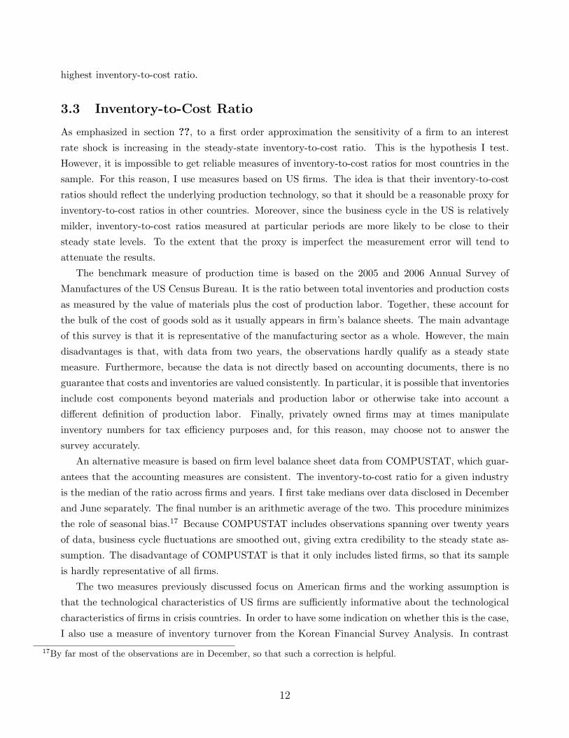
3.3 Inventory-to-Cost Ratio
As emphasized in section ??, to a first order approximation the sensitivity of a firm to an interest
rate shock is increasing in the steady-state inventory-to-cost ratio. This is the hypothesis I test.
However, it is impossible to get reliable measures of inventory-to-cost ratios for most countries in the
sample. For this reason, I use measures based on US firms. The idea is that their inventory-to-cost
ratios should reflect the underlying production technology, so that it should be a reasonable proxy for
inventory-to-cost ratios in other countries. Moreover, since the business cycle in the US is relatively
milder, inventory-to-cost ratios measured at particular periods are more likely to be close to their
steady state levels. To the extent that the proxy is imperfect the measurement error will tend to
attenuate the results.
The benchmark measure of production time is based on the 2005 and 2006 Annual Survey of
Manufactures of the US Census Bureau. It is the ratio between total inventories and production costs
as measured by the value of materials plus the cost of production labor. Together, these account for
the bulk of the cost of goods sold as it usually appears in firm’s balance sheets. The main advantage
of this survey is that it is representative of the manufacturing sector as a whole. However, the main
disadvantages is that, with data from two years, the observations hardly qualify as a steady state
measure. Furthermore, because the data is not directly based on accounting documents, there is no
guarantee that costs and inventories are valued consistently. In particular, it is possible that inventories
include cost components beyond materials and production labor or otherwise take into account a
different definition of production labor. Finally, privately owned firms may at times manipulate
inventory numbers for tax efficiency purposes and, for this reason, may choose not to answer the
survey accurately.
An alternative measure is based on firm level balance sheet data from COMPUSTAT, which guar-
antees that the accounting measures are consistent. The inventory-to-cost ratio for a given industry
is the median of the ratio across firms and years. I first take medians over data disclosed in December
and June separately. The final number is an arithmetic average of the two. This procedure minimizes
the role of seasonal bias.17 Because COMPUSTAT includes observations spanning over twenty years
of data, business cycle fluctuations are smoothed out, giving extra credibility to the steady state as-
sumption. The disadvantage of COMPUSTAT is that it only includes listed firms, so that its sample
is hardly representative of all firms.
The two measures previously discussed focus on American firms and the working assumption is
that the technological characteristics of US firms are sufficiently informative about the technological
characteristics of firms in crisis countries. In order to have some indication on whether this is the case,
I also use a measure of inventory turnover from the Korean Financial Survey Analysis. In contrast
17By far most of the observations are in December, so that such a correction is helpful.
12

to the measure based on the Annual Survey of Manufacturing, this gives equal weight to firms of
different sizes. The main advantage is that this avoids measurement error associated with idiosyncratic
decisions of very large producers, a particular problem in South Korea given its high rate of industrial
concentration. The turnover measure is defined as inventories/sales as opposed to inventories/costs,
which means that the numbers should be slightly smaller since sales are typically larger than costs.
Table ?? has the descriptive statistics for the three variables. The average production time is highest
in the COMPUSTAT sample, at 2.5 months, with a slightly smaller number for the Korean data.
Figure ?? shows the joint distribution between the Korean data (in the horizontal axis) and the two
US based measures (in the vertical axis). There is a reasonable amount of correlation between them,
between 0.5 and 0.6, summarized in table ??. The correlation between the Korean and American data
implies that taking US numbers as representative of other countries may not be so off the mark.
3.4 Controls
In this section I describe the controls. I include controls that account for a large range of alternative
forces that may lead to a sectoral reallocation. These are important to the extent that they are
correlated both with the inventory turnover ratio and the change in value added in the crisis period.
Table ?? has the descriptive statistics for the control variables. Table ?? has the correlations with the
dependent variables. In what follows, I discuss each one of them in detail.
3.4.1 Demand Side
Industries that specialize on investment or durable goods should be more impacted in a crisis since the
demand for these products is more pro-cyclical.18 On the other hand, firms that are export oriented
should experience a smaller drop in output.
I infer the share of output that is destined to the production of exports, investment goods and
durable consumer goods using input-output matrices made available by OECD.19 To measure the
demand for durable consumer goods consumption, I assume that all the consumption from certain
sectors is durable.20 I use country specific input-output matrices whenever possible, otherwise I
use an average for the region.21 I allow for indirect demand effects through the supply chain. As
a consequence, the control variable takes into account that the demand for basic metals is heavily
affected by the demand for investment goods.
18see, for example, the behavior of investment described by Calvoetal:2006b.19Thus basic metals are destined to the production of investment goods even though this only occurs indirectly. The
Leontief inverse gives the indirect destinations of output.20I define as durable consumption all the consumption of wood products, furniture, non-metallic mineral, machinery and
equipment and likewise use the Leontief inverse to account for indirect effects.21Thus, for example, the input-output structure for Malaysia is the average between South Korea and Indonesia.
13
3.4.2 Cost
During a sudden stop, there are massive realignments in relative prices. One particular case of interest
are imported inputs, which usually become more expensive. In the opposite direction, the reduced
demand for labor in a crisis should reduce wages. To capture these effects I include the share of labor
and imported inputs into production. For completeness, I also include a control for material share.
This is interesting since firms with high share of materials will have less sunk costs and will be more
willing to adjust its production to new circumstances.
3.4.3 Normal Cyclicality
The results may not capture the particular effect of the sudden stop, but just the usual effect of a
downturn. To proxy for the typical cyclicality of an industry, first I regress the growth in output of
each country/industry on GDP using overlapping three year windows as my observations but excluding
the 3 year period included in the left hand side of the main regression. I then collect the coefficients
and average them over industries. footnoteI also experimented with a measure of cyclicality based
only on US data. The results are largely similar, and are available upon request.
3.4.4 External Dependence
Rajanzingales:1998 define External Dependence as
External Dependence =Capital Expenditure - Cash Flow
Capital Expenditure
They calculate averages of this ratio for listed firms in the US. Rajan and Zingales argue that
the ratio captures technological aspects of production, in particular, the extent to which investment
is front-loaded when compared to production. Everything else constant, if access to finance is more
expensive, industries that require more up-front investment should do relatively worse. Dellaric-
cia:2007 and Kroszneretal:2006 have applied this insight to banking crises, and they find an important
role for external dependence. For comparability, I use the same numbers for external dependence as
Rajanzingales:1998.
3.4.5 Size
The empirical corporate finance literature has often focused on size as a determinant of differences in
the supply of finance available to different firms.22 Firm size may also matter because large firms are
more likely to be exporters.23 The UNIDO dataset has data on employment and number of establish-
ments by industries. I calculate for each country/industry pair the average employment/establishment
22See Fazzarietal:1988 for the seminal paper and GertlerGilchrist:1994 for an application specific to interest rate shocks.However, see also Kaplanzingales:1992 for a critique.
23See Melitz:2003.
14

ratio.24
3.5 Results
Table ?? shows the regression results with the turnover ratio from the Annual Survey of Manufacturing
as the dependent variable. Each column corresponds to a different measure of the turnover ratio. The
results are consistent and, for the measures based on US firms, statistically significant. The coefficient
on the turnover ratio of Korean firms is slightly higher. This is because for Korean firms the data
corresponds to inventory-to-sale ratio and sales are larger than costs.
The results for the controls are interesting in themselves. Most of them have the expected sign,
with exception of external dependence, which is positive, and the wage share, which is negative. The
coefficient on wage share is surprising, since it is highly statistically and economically significant. A
standard deviation change in the wage share implies a drop of 4.3% in output, which is an effect of the
same order as the inventory turnover. The exact reason for this coefficient constitutes a puzzle. One
possible explanation is that there are lags between the training and hiring of workers and production
of goods which are not adequately captured by inventories. Also, the evidence sits in nicely with the
suggestion by NeumeyerPerri:2004 that an interest rate shock increases primarily the cost of labor
input.
3.5.1 Sub-samples
Crisis episodes were heavily concentrated in certain time periods and geographic regions. About half
of the crises in the sample took place in the early eighties and the other half between the mid to late
nineties (and Argentina in 2001). Geographically, about half of the crises were in Latin America and
the rest distributed between Asia, Africa, Russia and the Middle East. I assess whether the coefficient
on the inventory-to-cost ratio is robust to splitting the sample in different ways.
The results are in table ??. The point estimate of the coefficient on inventory-to-cost ratios is
remarkably robust. For the US based measures, the coefficient is robust in 5 out of 8 cases. Given
that samples are half the size, it is not surprising that the statistical significance is reduced.25
The robustness of the coefficients is specially interesting, since in the early eighties, the crises
were followed by a much larger increase in inflation than in the nineties. The results provide further
evidence that cash-in-advance constraints were not playing an important role in production decisions.
3.5.2 Alternative time windows and persistence
A further robustness check involves changing the window over which I consider the drop in output.
The results are summarized in table ??. In the first rows I shorten the window by using a year closer
24I also experiment with the employment/establishment ratio in the year before the crisis. The results are virtuallyidentical.
25I have also run regressions that only include East Asian countries. However, there are only four of those in the sample,Korea, Malaysia, Thailand and Indonesia. The standard errors become even larger and the results unstable.
15
to the trough as the benchmark. The coefficients are robustly negative, although they tend to be less
significant and the coefficient smaller. As mentioned above, shorter time windows include cases where
the crisis was already under way in the initial year. Furthermore, estimates based on shorter windows
are likely to be more noisy, which by itself should imply larger standard errors.
The windows in the last two rows compare value added three years before the trough of the crisis
with, respectively, three and five years after the trough. The coefficients provide information about
the persistence in the reallocation once the recovery has taken place. The somewhat surprising result
is that the reallocation is quite persistent. This is important because it indicates that the findings are
most likely not associated with short-term inventory adjustment. Given a total inventory turnover
ratio of less than three months and an even smaller number as far as finished goods inventories are
concerned, these dynamics should have been exhausted once the recovery is under way.26
4 Quantitative Model
4.1 Model Setup
The model economy has multiple sectors, allowing for investigation of the impact of different shocks
on the cross-section of industries. In particular, it has NT tradable sectors corresponding to manufac-
turing sectors. Since this is a general equilibrium model, I also allow for NNT non-tradable sectors in
order to have a comprehensive depiction of the economy.
4.1.1 Household
Let st denote the history of states of nature up to time t. There is a representative household who
takes prices as given and is able to borrow and lend abroad at an exogenous riskless gross interest rate
er(st). The household supplies labor and consumes both durable and non-durable goods. The utility
function of this household is time-separable with period utility given by
u(C
(st
),KH
(st
), L
(st
))=
11− σ
[γd 1ρC
(st
) ρ−1ρ +
(1− γd
) 1ρKH
(st
) ρ−1ρ
] ρρ−1
−L
(st
)1+ 1ψ
1 + 1ψ
1−σ
Where C(st
)is non-durable consumption and D
(st
)is the stock of durable goods held by the
household, L(st
)is labor supply.
This utility function follows GHH:1988. Its essential property is that the labor supply does not
respond to wealth of the household, only to wages. One motivation is that labor supply is costly
26In particular Alessandriaetal:2008 study the implications of inventory adjustment dynamics for the response of importsand import prices in the aftermath of devaluations. They find large effects which, however, exhaust themselves in less thana year.
16

because it implies a loss in output from home production or self employment. Such an interpre-
tation is particularly suitable for developing countries, where a large fraction of the population is
self-employed.27
4.1.2 Production Functions
The production function of each sector is:
Y i(st
)=
τ i∏v=0
Zi(st−v, v
)ωi(v)∑
ωi (v) = 1
Where Yi is the production of the input i. Zi(st−v; v
)denotes a composite of goods acquired in
period t− v to produce the finished good which is sold v periods ahead. It is defined as:
Zi(st, v
)= γiea(s
t) (ui
(st; v
)Ki
(st; v
))αiK (Li
(st; v
))αiL (Mi
(st; v
))1−αiL−αiK
Where ui(st−1; v
)denotes the rate of utilization of fixed capital at t.
4.1.3 Capital Accumulation, Utilization and Maintenance Costs
Capital is sector specific and is produced by combining old capital and investment goods:28
Ki
(st
)=
[(1− δKi
) (Ki
(st−1
)) ζ−1ζ +
(δKi
) 1ζ
(Ii
(st
)) ζ−1ζ
] ζ−1ζ
Durable consumer goods are produced in a similar fashion:
KH
(st
)=
[(1− δD
) (KH
(st−1
)) ζ−1ζ +
(δH
) 1ζ (IH
(st
)) ζ−1ζ
] ζ−1ζ
Whenever a firm uses capital, it has to make up for wear and tear. This maintenance requirement
is increasing in capacity utilization. The required spare parts satisfy:29
27The motivation for strong wealth effects in labor supply relies to a large extent on the observation that there is not aclear long run trend in average hours worked [?]. However, there is a clear increase in labor force participation in emergingmarket economies. See, for example, Young:1995 for the Asian Tigers.
28
Let Ki(st) = K(I(st),K(st−1)
). The parametrization below is such that G satisfies the following conditions:
K = K (δK,K) ,∂K (δK,K)
∂I= 1,
∂K (δK,K)∂K
= 1− δ
29In the calibration, I choose units so that in steady state u = 1 and the firm does not have maintenance costs. If capacityutilization is below steady state, the firm has spare parts, that they can sell at market prices for alternative uses. This
17
Ωi
(st
)=
χ
1 + ξ
[ui
(st
)1+ξ − 1]Ki
(st
)4.1.4 Composite Goods
Non-durable consumption C(st
), fixed investment Ii
(st
), durable consumption good investment
IH(st
), materials Mi
(st
)and spare parts Ωi
(st
)are composites of the goods produced in the
NT +NNT sectors and imported goods. These composites are represented by CES aggregates:
X(st
)=
∑j∈1,...,NT+NNT
(γjX
) 1ρ (Xj
(st
)) ρ−1ρ
+(1−
∑j∈1,...,NT+NNT γ
jX
) 1ρ (X∗ (
st)) ρ−1
ρ
ρρ−1
Where X stands in for C, Ii, Ωi or Mi. X∗ (st
)is the amount of imported goods used for the
production of X and∑γiX < 1.
4.1.5 Foreign Trade
While the economy is small with respect to capital markets, it is large relative to product market. This
is the case, for example, if countries produce different varieties that are not perfect substitutes.30 This
assumption implies that tradable sectors have to respond at least somewhat to changes in domestic
demand.
The tradable sectors face the following inverse demand function:
pi(st
)= χi
[EXP i
(st
)]− 1θ
Where pi(st
)is the price of good i with respect to the foreign good and EXP i
(st
)are exports of
sector i good. I assume that services, construction and real estate are non-tradable.
For the tradable sectors, exports are identical to the total output from sector i minus the sum of
the domestic demands for this good:
EXP i(st
)= Y i
(st
)− Ci
(st
)− IiH
(st
)−
∑j∈1,...,NT+NNT
(M ij
(st
)+ Iij
(st
)+ Ωi
j
(st
))For non-tradables, exports are equal to zero:
EXP i(st
)= 0 if i is non-tradable
assumption is made for tractability, but does not have any important consequence.30It is a common assumption in the literature. See GertlerGilchristNatalucci:2007 and KehoeRuhl:2008. Note that this
does not imply monopolistic power if many producers in a country produce the same variety. All that is required is that thecountry be sufficiently big relative to the world demand for that variety.
18

Total imports are the sum of all foreign goods demanded for different uses:
IMP(st
)= C∗
(st
)+ I∗H
(st
)+
∑j∈1,...,NT+NNT
(M∗j
(st
)+ I∗j
(st
)+ Ω∗
j
(st
))I take these foreign goods to be the numeraire, so that their price is identical to 1. The current
account identity is:
B(st
)−R
(st−1
)B
(st−1
)= IMP
(st
)−
∑i∈1,...,NT
pi(st
)EXP i
(st
)Where B
(st
)is the amount of net foreign debt held by domestic households.
4.1.6 Resource Constraints
While capital is sector specific, its utilization can be shuffled around for the production of goods to
be finalized at different horizons. This implies the following resource constraint for capital stock for
sector k:
∑v
ui(st; v
)Ki
(st; v
)≤ ui
(st
)Ki
(st
)Raw materials respect an analogous resource constraint:
∑v
Mi
(st, v
)≤Mi
(st
)In contrast, labor is perfectly mobile between sectors. This implies the following labor market
clearing condition
∑k∈1,...,NT+NNT
n∑v
Li(st, v
)≤ L
(st
)Finally, there is a market clearing condition in the non-tradable sectors. This is:
Ci(st
)+ IiH
(st
)+Gi +
∑j∈1,...,NT+NNT
(M ij
(st
)+ Iij
(st
)+ Ωi
j
(st
))≤ Y i
(st
)Where Gi are government purchases, assumed to be constant over time.
19

4.1.7 Equilibrium
The economy has a representative household and there are no frictions or missing markets. This
implies that the allocation can be computed as the solution to a planner’s problem. However, this has
to be modified so that the planner does not internalize the impact of choices on pi(st
). Otherwise, the
planner would use market power in the foreign goods market to increase the welfare of home house-
holds at the expense of foreign households. Such coordination is unlikely to occur in a decentralized
equilibrium.
The equilibrium is defined as follows: The social planner takes the functionspi
(st
)k∈1,...,NT
as
given and chooses all remaining functions of st to maximize household welfare subject to technological
and resource constraints described above. The equilibrium is the solution to the planner’s problem
andpi
(st
)k∈1,...,NT
so that for all st,pi
(st
)k∈1,...,NT
=χi
[EXP i
(st
)]− 1θ
k∈1,...,NT
.
4.2 Calibration
4.2.1 Sectors and Shares
The first task is to assign empirical counterparts to the different sectors. I use an average of the
input-output tables in section ??. To do this, first I normalize the entries in each of the tables to total
production in the country. I then average over all of them. the resulting” input-output table has 48
sectors which I aggregate into 20 as follows:
First, I aggregate all the non-manufacturing sectors into three non-tradables: construction and
real estate and a large, residual, “service” sector that includes services, retail, utilities, public admin-
istration and agriculture. I treat mining as a foreign sector since it is highly tradable and employs
very little.31
Singling out the construction sector is interesting because its long production time has motivated
the introduction of time to build technology by Kydlandprescott:1982. It is potentially very important
in so far as aggregate dynamics are concerned. The real estate sector, in turn, is included to absorb
the output of the construction sector. The real estate sector allows the model to have a large and
important construction sector without exaggerating the importance of this type of capital in the
remaining production activities.
As far as the manufacturing sectors are concerned, I assign to each one of them an ISIC Rev. 2 code
in order to be able to match to the data in the emprical section. The correspondence is not perfect.
Some sectors that are differentiated in the empirical section, such as textiles and apparel, only appear
as a single sector in the input-output matrix. On the other hand, the input-output matrix includes
more machinery producing sectors than in the UNIDO data-set. In this latter case, I consolidate the
sectors in order to build equivalents to the ones in section ??.
The sectors that I treat as non-tradable do, as a matter of fact, trade. I treat all their sales abroad
as domestic sales and all the purchases from their counterpart abroad as domestic purchases. I am
31I also experimented with treating agriculture the same way as mining. The results are not sensitive to this assumption.
20

still left with a (small) imbalance. Also, at the aggregate level there is a trade imbalance that does
not come up in the steady state of the model. I remove these imbalances by rescaling the size of the
non-tradable sector and of domestic absorption.
I rescale the labor shares up by a factor of 2, conforming to the findings in Young:1995 and
Gollin:2002 that labor shares in developing countries are frequently underestimated because of the
large number of self-employed workers. This brings the aggregate labor share close to 0.6, which is
the norm of developed countries. Also, I do not allow explicitly for indirect taxes in the model, so that
I split them between labor and capital income.32 Given the input-output table, it is a straightforward
matter to calculate the factor shares for the different sectors as well as the weight of each sector in
each of the different composite goods.33
4.2.2 Time to Produce
I calibrate the production process in each sector as follows. First, for the manufacturing sectors, I set
Y i(st
)= Zi
(st, 0
)1−ωiZi
(st−1, 1
)ωiI choose ωi for each sector so that the inventory-to-cost ratio matches the numbers constructed
from the Annual Survey of Manufacturing.34
The production function for services and real estate sectors is simply:
Y i(st
)= Zi
(st, 0
)Finally, for the construction sector,
Y Const.(st
)= ZConst.
(st, 0
) 14 ZConst.
(st−1, 1
) 14 ZConst.
(st−2, 2
) 14 ZConst.
(st−3, 3
) 14
Counter-Factual Calibrations: For the sake of comparison, I also include some counter-factual
calibrations. I assume that all manufacturing sectors produce instantaneously, so that
Y i(st
)= Zi
(st, 0
)∀i ∈ 1, NT
4.2.3 Export demand, capital accumulation and maintenance cost
The crucial parameter in the demand for net exports is the price elasticity, θ. In fact, the literature on
emerging market business cycles has diverged dramatically on the appropriate value for this parameter,
32For an interesting account of how heterogeneity in indirect taxes provides a foundation for fluctuations in TFP, seeBenjaminMeza:2009.
33The only slight difficulty is in making sure that factor shares reflect the heterogeneity in opportunity cost of capital facedby the different sectors.
34For sectors which encompass more than one sector in my data-set, I pick the number corresponding to the one withrelatively larger value added.
21

with some papers setting it as low as 1 or 2 and many other papers assuming that the economy
is small in the goods markets, so that, effectively, θ → ∞. Econometric estimates diverge, with
Mendoza:1994 finding that there is no Granger causation running from exports to terms of trade, and
SenhadjiMontenegro:1998 estimating price elasticities of export demand as low as 1.5. More relevant
to the present work, Bursteinetal:2005 show that, over some important cases of large exchange rate
depreciations the price of traded goods at the dock dropped very little in foreign currency terms,
which suggests a high elasticity of demand for exports. I use θ = 20 as my benchmark and, in the end
of the paper, present sensitivity analysis with θ = 2 and θ = 200.
For the capital accumulation equations, I set the depreciation of fixed capital δK equal to 10%
yearly for all sectors but real estate. The depreciation rate for the capital of the real estate sector
I set to 2.3% yearly. Finally, the depreciation of durable consumer goods δH to 13%. These values
approximate the rate used by the Bureau of Economic Analysis to depreciate stocks of physical assets
in the US economy.
To calibrate maintenance cost, I set ξ = 0.5 and µ set such that in steady state ui(st
)= 1. As
far as the share parameters are concerned, I assume that they are identical to the investment good,
except that I exclude output from the construction sector.
The remaining parameter is the elasticity of investment to the replacement cost of capital, ζ. This
is hard to calibrate, so that I allow the model to pick it jointly with the interest rate and TFP shocks
(see discussion below).
4.2.4 Remaining Parameters
For the household preferences, there are three parameters to be calibrated, ψ, σ, ρ. I follow Men-
doza:1991 and UribeYue:2006 and take ψ = 2.28 and σ = 2. The household discounts the future at a
rate β. I set that to be equal to 1R in steady state, and choose R so that the steady state interest rate
is 3.5%.
I assume ρ = 2, so that the output of different sectors are substitutes.
4.2.5 Exogenous processes and adjustment costs
The exogenous state determines the path of interest rates, productivity, and foreign demand for
domestic inputs. These are described by the following auto-regressive processes:
r(st
)= (1− ηr) r + ηrr
(st−1
)+ εr (st)
a(st
)= ηaa
(st−1
)+ εa (st)
I pick the steady state interest rate r to match the ratio between investment and total output.
This is about 8.49% per year, which is consistent with the interest rates often observed in emerging
markets.
22
I model the crisis as a simultaneous, one-time shock to both processes. In order to calibrate the
magnitude of the shocks and the persistence parameters, I use the average deviation from trend of
output and capital formation across the crises episodes. In particular, I require that the model matches
the average drop of GDP and fixed capital formation in the trough of the crisis, and that it matches
the change in the deviation from trend in the two years after the trough.35 The calibration targets
are depicted in figure ??. Note in particular that investment drops much more than GDP and that
both series remain fail to revert to their previous trend.
The calibrated parameters are highly dependent on the importance of adjustment costs. If adjust-
ment costs are high, the same drop in investment relative to output will require a larger increase in the
interest rate. Since adjustment costs are particularly important for the short term dynamics of invest-
ment following a shock, I use available quarterly data on investment and GDP from UribeYue:2006.
Their dataset includes information on six episodes which are included in the events studied in this
paper.36 The exact quarter in which the crisis starts is easy to identify. It is the quarter close to the
trough of the crisis in which there was a large increase in the trade balance. As the calibration target,
I use the ratio of average investment/GDP ratio in the trough of the crisis to its value in the first
couple of quarters after the shock.37 This calibration target is depicted in figure ??.
The calibration based on investment and GDP series is preferable to the use of direct measures of
the interest rate and TFP. Interest rates in emerging markets can be a poor measure of the marginal
cost of funds faced by agents in these economies, specially around times of crisis. On the one hand,
interest rates may reflect risk premia that, per se, do not add to the marginal cost of funds. On the
other hand, many of the crisis economies had fairly regulated financial systems to begin with. From
that perspective, the interest rate could actually be an underestimate of the marginal cost of capital.38
As for TFP, an accurate measurement requires the calculation of hours data which, for most of these
countries, is not available.
The calibration implies a very persistent interest rate shock (ηr = .99) , high adjustment costs
(ζ = 0.91), and a TFP shock that mean-reverts relatively quickly (ηa = .91). The persistent interest
rate is necessary to account not only for the persistence of investment and of GDP, but also in the
drop in the investment/output ratio.
I solve the model by log-linear approximation around the non-stochastic steady state. This is
necessary because of the large number of state variables.39
35See details in Appendix C.36Argentina (2001), Ecuador (1999), Malaysia (1998), Mexico (1995), South Korea (1999), and Turkey (1998).37See details in Appendix C.38Naturally, this discussion suggests that the implicit restriction that all sectors in the economy face the same interest rate
may not be appropriate. Investigating the role, if any, that such a heterogeneity is an important direction for future work.39I solve the model using Dynare.
23

4.3 The Effect of Shocks
This section studies the effect of exogenous shocks in the economy described above. I show the
results for aggregate GDP, gross capital formation and cross-sectoral output. The central purpose
is to understand the role of the time-to-produce technology. In order to emphasize this, I use the
calibration for the exogenous shocks and capital adjustment cost parameters used in the full model.
Figure ?? shows how output and investment react to the shocks under the different assumptions
concerning the existence of time to produce. In order to facilitate the comparison I do not recalibrate
the shocks and adjustment cost parameter for the different models. The interest rate shock is very
persistent, which, in turn, implies a persistent reaction of GDP and investment. In effect, GDP
is declining over time as fixed capital is progressively reduced. In contrast, the reaction of GDP
and investment to the TFP shock are clearly mean-reverting, in line with the mean reversion in the
exogenous shock itself.
Over the long run, interest rate shocks are most potent in the full model. This is not surprising,
since the models without time to produce has one less channel through which the interest rate can
affect output. Interestingly, there is not a discernible difference between models in the reaction to the
TFP shock.
The most interesting differences between the models are in the first couple of quarters following the
shocks. First, they highlight the role of sunk costs in generating delayed responses. Because in both
models there is time-to-build in the construction sector, investment decreases only slowly in the first
four quarters. This is because it is optimal to conclude building projects that were initiated before the
shock hits given that a large part of the requisite effort has already been made.40 A similar dynamic
is visible in the response of GDP to a TFP shock. Instead of dropping immediately and then slowly
recovering, GDP follows a hump-shaped response pattern.
The final result is that, over the first couple of quarters, GDP responds most strongly to an interest
rate shock if manufacturing production takes time. The reason is that, absent production lags, over
the short run manufacturing sectors are very little affected by the interest rate shock. In effect,
they benefit from lower wages and lower price of non-tradable inputs. The possibility to reallocate
labor from non-tradable towards the tradable sector allows the economy to adjust to the interest
rate shock without much initial pain. The result is reminiscent of the findings by KehoeRuhl:2008
and Charikehoemagrattan:2005.41 The interest rate shock does become important over the longer
run for all models, as fixed capital gets depleted. Once time-to-produce is allowed for, firms in the
manufacturing sector react to the interest rate shock with a reduction in output, since now their
40In the model, fixed investment is only accounted for once the final good is ready to be incorporated into the capitalstock. According to the 1993 System of National Accounts, “The time at which gross fixed capital formation is recordedis when the ownership of the fixed assets is transferred to the institutional unit that intends to use them in production.”(http://unstats.un.org/unsd/sna1993/toctop.asp, Ch. 10-B). Thus, the procedure is adequate if in the economies underconsideration all construction activity is performed by institutional units other than the ones who actually use the buildings.This is unlikely to be the case, but it is a better assumption than that all construction is made in house.
41Although in these papers, the counter-intuitive results are made even more dramatic because the authors allow for wealtheffects on labor supply.
24
production costs have increased. Note that the difference between the two models is visible even in
the first quarter, since value added includes the change in inventories, itself a forward looking variable.
Finally, the scatter plots in figure ?? shows the deviation from trend in the value added of each
sector, averaged over the trough of the crisis. The first row depicts results for the full model, whereas
the second row has the results for the model where time to build is only prevalent in the construction
sector. The TFP shock has mainly a level effect, with very little implications for the cross-section
in either model. In contrast, in both models the interest rate shock generates a reallocation in the
direction shown by the data. However, the reallocation is much stronger in the model with production
time in manufacturing.42
4.4 Comparison with Data
Figure ?? compares output in different sectors in the trough of the crisis in the data with what both
the full model and the model where manufacturing sectors produce instantaneously. The data for each
industry refers to an average across countries of the difference between their current output and their
previous trend.
Overall the model generated data tends to over-estimate the performance of manufacturing sectors
relative to the data, as demonstrated by the higher intercept of the regression curves. The model fares
much better is in capturing the slope of the regression line, which I take as a measure of the reallocation
towards sectors with low inventory-to-cost ratios. This is most visible in figure ??, where the data-
points correspond to deviations from means, so that all regression lines have the same intercept. Note
that the model without time to produce in manufacturing has a much flatter slope.
In what follows I discuss the results in more detail, with special attention for the role of different
parameters.
4.4.1 Reallocation from Tradables to Non-Tradables
The average drop in manufacturing is, in the data, larger than the drop in overall GDP.43 44
Table ?? shows the average deviation from steady state of output in the manufacturing sector
relative to the deviation from steady state of GDP given different parametrizations of the full model
(to facilitate the comparison, I do not recalibrate the persistence and magnitude of the shocks and the
42The major reason there is a reallocation in the model without production time is because there is a correlation betweenorientation towards the production of investment goods and production time. The slope goes away once this correlation iscontrolled for.
43This empirical finding stands in contrast to the findings by TornellWestermann:2002 who document that, in the aftermathof emerging market crises, there is a reallocation from non-tradable to tradable production. To a large extent the discrepancyhas to do with aggregation: manufacturing sectors that fall least also respond for a larger share of manufacturing production.In contrast, I weight all sectors equally in this exercise.
44A similar problem occurs in KehoeRuhl:2008 model of sectoral reallocation in the Mexican crisis. While the authorsclaim success in generating a reallocation towards tradable production, the reallocation implied by the model is much largerthan the one they find in the data.
25

capital adjustment cost parameter). Higher numbers imply that the model predicts that manufacturing
drops relatively more when compared to overall GDP.
When compared to the model where production in the manufacturing sector is instantaneous, the
full model does somewhat better. This is not surprising, since if production is instantaneous, the cost
of manufacturing production will not be directly affected by the interest rate.
The reallocation from non-tradables to tradables is much less pronounced if labor supply is more
elastic. The reason is that with inelastic labor supply, workers displaced from the non-tradable sector
move to manufacturing. If labor supply is elastic, it will be preferable for many of these workers to
stay at home rather than have a low labor productivity in one of the manufacturing sectors.
Another interesting parameter is the elasticity of foreign demand for exports. The relative gains
for the tradable sector are least if this elasticity is low. This is fairly intuitive. With a low elasticity
of demand, there is less to be gained by increasing exports.
Finally, the output loss in the manufacturing sector is relatively larger if capacity utilization costs
are close to linear. The reason is that, with linear capacity utilization costs, small changes in costs
have a large impact on output.
4.4.2 Reallocation within Manufacturing
Where the benchmark model does a much better job is in replicating the reallocation pattern within
manufacturing. This can be seen from the slope of the regression line in the model, which is only
slightly smaller than that for the data. In contrast, the model without production time among
manufacturing industries does a much poorer job. To the extent that it does imply a negative slope,
this is a consequence of other cross-industry differences, such as export orientation.
In order to isolate the role of production time, I regress the model generated data on model
equivalents of the controls included in the regressions in the empirical section of the paper. I use all
the sources of cross-sectoral heterogeneity which are explicitly modeled, leaving out establishment size,
external finance dependence and cyclicality. Table ?? show the estimated coefficient for the inventory-
to-cost ratio in the model, given different parametrizations. The coefficient in the benchmark model
is smaller than in the data, but still within the confidence interval. In contrast, in the model where
production in the manufacturing sector is instantaneous, the coefficient becomes positive.
As far as alternative parametrizations are concerned, the most interesting results are linked to
assumptions about the price elasticity of foreign demand for domestic exports. In order to get a
quantitatively meaningful cross-sectoral reallocation it must be the case that this elasticity is high. If
it goes down to 2, very little cross-sectoral reallocation occurs. The reason is that final price changes
would countervail the impact of the interest rate shock on production costs.
4.4.3 Initial Impact
One important issue for the emerging market literature is the extent to which a sudden capital flight
can in and of itself generate an immediate drop in output. To a large extent, this preoccupation
26

is behind NeumeyerPerri:2004 modeling decisions and Charikehoemagrattan:2005 critique. In the
context of this model, the question is to what extent the interest rate shock alone can account for the
initial drop in output immediately following the crisis shock.45
In the benchmark calibration, the interest rate shock accounts for more or less 25% of the drop
in output in the quarter when the shock hits and the following one. This is substantial, but not
overwhelming. However, it is much larger than what is obtained if there is no production time in the
manufacturing sectors, which is essential zero. The reason is that, absent production time, the planner
can move resources away from the non-tradable sectors towards tradable production in response to
an interest rate shock, so that the resulting movements in demand have very little effect on output.
Also, any effects on the supply side only accrue over longer periods of time, as the fixed capital stock
is depleted.
With time to produce, savings are needed not just to fund fixed investment, but also to fund
variable investment, in the form of materials, labor input and spare parts needed to make up for
capital utilization. Because the maturity time of this form of investment is much shorter, the results
are felt almost immediately.
As far as alternative parameters are concerned, again the most interesting ones are the ones
concerning the price elasticity of exports. The role of the interest rate is largest when the price
elasticity of exports is low. In this case, the planner cannot easily make up for the reduced domestic
demand by increasing output in the exporting sectors since this attempt will be met by increased prices.
Note, however, that in this case a completely different mechanism is at play. While interesting, such a
mechanism is inconsistent with the cross-sectional evidence since, as discussed in section ??, such low
elasticities would imply an inability of the model to generate a pattern of cross-sectoral reallocation
consistent with the data.
5 Conclusion
This paper proposes that production time is an important propagation mechanism for interest rate
changes. It partly accounts for two observations about emerging market economies: that shocks to
the interest rate have a strong and swift impact on output and that in crisis episodes there is a
substantial reallocation towards industrial sectors that use few inventories relative to their costs. It is
similar to NeumeyerPerri:2004 payment-in-advance constraint in so far as the aggregate implications
are concerned, but it is also able to account for cross-sectional facts.
The paper opens up some important avenues for research. First, it highlights the importance of
understanding the role of variable capital investment in order to understand emerging market crises.
While this role was previously emphasized by NeumeyerPerri:2004 as a means to generate reasonable
time-series behavior out of for a Small Open Economy RBC model, as it turns out something along
these lines is also necessary to generate the requisite cross-sectoral behavior. The particular form of
45Such a decomposition is possible because the model is solved using a linear approximation.
27

variable capital emphasized in this paper, summarized in the inventory-to-cost ratios, is interesting in
that it is relatively straightforward to measure and is associated with real quantities. As a consequence,
it does not rely on frictions which are hard to measure and to motivate.
One direction for further work which is closer to the spirit of NeumeyerPerri:2004 contribution
is to investigate the special role of the wage-bill. The regression results imply that labor intensive
industries did relatively worse in the crises, when everything else is constant. This is, on the face of it,
a counter-intuitive finding, that deserves further exploration. One possibility, which is in line with the
argument in this paper, is that labor includes administrative work, which has a longer time horizon
than labor directly applied to the production process. More generally, the need to train new workers
and other costs of hiring may have similar implications. Allowing for a richer labor market structure
seems to be an interesting way forward.
The second avenue for research is an exploration of the links to the credit friction literature. In
the paper, I take the cost of capital as given and look at the effects on production, while much of the
literature does the opposite. The question is whether there is some important insight to be gained by
combining the two. This is specially likely to yield interesting results if credit frictions operate at the
level of the firm, as in currency mismatch models or if the crisis is understood primarily as a failure of
the banking system in channeling funds from consumers to firms.46 In these cases, a mechanism that
operates specifically through the supply is important in order for these frictions to have important
role in so far a short term output dynamics are concerned.
Third, it is worth asking what the results tell us about developed economies. There is nothing, in
principle, that makes the mechanism more relevant to emerging markets than for developed countries.
Understanding whether there are important differences to be considered is in itself an important area
for further research.
Lastly, on a methodological note, the paper illustrates the fruitfulness but also some of the pitfalls
of exploiting cross-sectional data to shed light on macroeconomic mechanisms. On the one hand,
cross-sectional data add a whole new dimension of facts that can be used to discipline macroeconomic
models. On the other hand, counter-factuals based on cross-sectional analysis tends to ignore general
equilibrium effects, so that complementing these with a model is important to have a full appreciation
of the effects in question. More generally, the increasing ability to solve large multi-sector models and
availability of good quality cross-sectional data should allow for even richer explorations along these
lines in the years to come.
46In particular, christianogustroldos:2004 point out that a payment in advance constraint affect the calculus of optimalpolicy to deal with these frictions. It would be interesting to check whether introducing production time affects the result.More fundamentally, because production time can be traced to inventories and production technology this would allow for aquantitative assessment of christianogustroldos:2004 mechanism.
28

Appendix A: Value Added Accounting with Time to Pro-
duce
This appendix shows the implications of time to produce for value added accounting. The framework
is an extension of the partial equilibrium model in section 2. Because value added includes wages,
suppose the production function is
Yt =([Zt (1)]1−ω [Zt−1 (2)]ω
)φZt (v) = (Mt (v))
1−αL (Lt (v))αL
The numbers in parenthesis denote the distance in time between the acquisition of the input and
the sale of the output. Zt (v) is a composite of materials, Mt (v) and labor Lt (v)
Let qt be the price of raw materials and wt the wage rate. Then
V At = Yt − qt (Mt (0) +Mt (1)) + Invt −Rt−1Invt−1
Again, the definition above abides to the recommendation of the 1993 System of National Accounts
that inventories should be valued at current price.
Substituting in the various definitions:
V At = Yt − COGSt + wtLt (0) + wtLt (1)
Thus, value added is the sum of the profits of the firm and the wages dispensed to workers at time
t.
Note that, given perfect foresight, profit maximization implies that:
V At = (1− φ)Yt + φαL ((1− ω)Yt + ωYt+1)
While sales are determined by prior input choices, value added is not since it incorporates the
income of workers involved in the production of future output. Thus, the reaction of value added to
an interest rate shock is actually even quicker than that of sales. From t ≥ 2 onwards, if the interest
rate shock is persistent enough. value added behaves very much like sales and the comparative statics
on ω apply as before.
29

Appendix B: Inventory Turnover and Interest Exposure
with generic production function
This section extends the framework in section 2 to allow for generic production functions. Suppose
yt = f(Zt−v (v)Nv=0
)With f strictly increasing and concave. Consider the problem of a firm under perfect foresight.
The firm is deciding how much to produce at t with enough time to choose all the Zt−v (v).
To study the production decision of this firm, it is useful to define the accumulation function. This
is the appropriate rate to inflate past costs so that they are comparable with present gains. Call the
numeraire good a ”dollar”. If R (u) is the dollar interest rate between periods u and u+1, then, under
perfect foresight, the accumulation function is
Γt−v (v) ≡t−1∏
u=t−vR (u)
The cost minimization problem for the firm is:
min∑v
Γt−v (v) qt−vMt−v (v)
s.t. : f(Mt−v (v)Nv=0
)≥ yt
Consider the impact of a permanent interest rate shock (that is, with η → 1). This will affect
Γt−v (v). Application of the chain rule combined with Shephard’s lemma implies that:
dC(yt, Γt−v (v) , qt−vNv=0
)C
(yt, Γt−v (v) , qt−vNv=0
) =∑ Γt−v (v) qt−vzt−v (v) v∑
u Γt−u (u) qt−uzt−u (u)dR
R
It is straightforward to show that, in steady state, coefficient multiplying dRR in the right hand side
is exactly equal to the ratio between inventories and costs.
30

Appendix C: Details of Calibration
In order to calibrate the model I use yearly data on output and investment for 21 episodes in my
sample and quarterly data for 6 countries (Argentina, Ecuador, Korea, Mexico, Malaysia, Turkey).
I start by specifying the targets based on the yearly data. Let t∗ denote the trough of GDP
as identified by Calvo et al. (2006). First, for each time series, I calculate the deviation from the
projection a of linear trend estimated using the data from t∗−9 to t∗−3 (I use log values for GDP and
gross fixed capital formation). I then average across all the 21 episodes to get the average deviation
from trend.
In order to perform the comparison to the calibrated data, I have to time aggregate it. I also have
to take into account that there are different possible quarters in which the crisis may have started so
that the trough of GDP falls in year t∗. In particular, the simulations imply that this will be a case
for crises starting in any quarter from March t∗ − 1 to January t∗. Thus, the model counterpart of
output in year t∗ is an average across crises whose starting dates correspond to these different cases.
Let GDP t and It correspond, respectively, to the average log deviations from trend of GDP and
investment in the yearly data. The calibration targets are GDP t∗ , It∗ , GDP t∗+2−GDP t∗ , It∗+2− It∗ .The last calibration target exploits information in quarterly data. For each of the 6 countries
for which I have the data, I calculate the difference between log investment and log GDP and then
calculate the deviation from the average value of this difference in year t∗ − 3. Denote the resulting
series by ıs. Let s denote denote the quarter corresponding to the onset of the crisis, identified as an
occasion close to the Calvo dates in which the trade balance increases by a historically large amount.
The investment to GDP ratio is at its lowest in s+ 5. The calibration target is ıs−1+ıs+ıs+1
ıs+4+ıs+5+ıs+6.
Denote the model counterparts of the different variables by removing the hats. I solve the following
minimization problem:
minηa,ηr,εa,εr
(GDPt∗ − GDPt∗
)2+
(It∗ − It∗
)2
+(GDPt∗+2 −GDPt∗ −
(GDP t∗+2 − GDP t∗
))2
+(It∗+2 − It∗ −
(It∗+2 − It∗
))2
+(
is−1+is+is+1
is+4+is+5+is+6− ıs−1+ıs+ıs+1
ıs+4+ıs+5+ıs+6
)2
For most of the cases, I am able to bring the loss function down to 10−5 and sometimes as low as
10−6. The bulk of the remaining error is normally concentrated in the(It∗+2 − It∗ −
(It∗+2 − It∗
))2
and reflects the difficulty of the model in generating a drop in investment even after the trough of the
crisis, as observed in the data.
31

311
313
321
322323
324
331
332
341
342
351 352
353354
355
356
361362
369
371
372
381
382
383
384 385390
−.4
−.3
−.2
−.1
0C
hang
e in
Val
ue A
dded
from
t*−
3 to
t*
1 2 3 4Inventory−to−Cost (Annual Survey of Manufacturing)
Mean change across crisesInventory−to−Cost and Change in Value Added
.
Figure 1: Change in value added averaged across crises episodes against inventory turnover for eachindustryThe change in value added is the log change in the three years leading to the trough of the crisis. Theturnover ratio is the ratio between total inventories and variable costs, calculated with data from theAnnual Manufacturing Survey for 2006. Industry data are published by UNIDO and refer to 3 digitclassifications according to ISIC Rev. 2.
32

311
313
321323
324
331332
341
342
351
352
353
354355
356
361
369
371
372
381
382
383384
385
390311
313
321
323
324331
332
341
342
351
352353
354
355
356
361
369
371
372
381382
383
384
385
390
01
23
4In
vent
ory/
Cos
ts (
US
A, m
onth
s)
.5 1 1.5 2 2.5Inventory/Sales (South Korea, months)
Annual Survey of Manufacturing (US) COMPUSTAT (US)
Inventory TurnoverMeasures of Time to Produce
Figure 2: Inventory Turnover MeasuresThe change in value added is the log change in the three years leading to the trough of the crisis. Timeto produce is the ratio between total inventories and production costs calculated based on data fromthe Annual Manufacturing Survey for 2006. Industry data are published by UNIDO and refer to 3 digitclassifications according to ISIC Rev. 2.
Country Year N Country Year N
Argentina 1982 28 Turkey 1994 28El Salvador 1982 27 Morocco 1995 27Brazil 1983 26 Mexico 1995 28Chile 1983 28 Indonesia 1998 27Mexico 1983 28 South Korea 1998 28Peru 1983 28 Malaysia 1998 28South Africa 1983 28 Russia 1998 28Cote d’Ivoire 1984 20 Thailand 1998 8Nigeria 1984 8 Ecuador 1999 28Uruguay 1984 28 Turkey 1999 28
Argentina 2002 28
Table 1: Crises EpisodesThe episodes are the same ones selected by Calvoetal:2006b, see text for details.
33

mean median min max stdevInventory-to-Cost (Survey of Manuf.) 1.97 1.77 0.76 3.43 0.66
Inventory-to-Cost (COMPUSTAT) 2.46 2.45 0.51 3.94 0.91Inventory-to-Sale (Korea) 1.60 1.61 0.61 2.61 0.44
Export 0.25 0.19 0.04 1.03 0.16Investment 0.22 0.13 0.00 0.87 0.21
Durable Cons. 0.08 0.03 0.00 0.41 0.09Cyclicality 1.36 1.38 0.49 2.43 0.47
Labor Share 0.14 0.14 0.02 0.31 0.06Materials Share 0.66 0.67 0.50 0.86 0.07
Import Share 0.12 0.10 0.02 0.75 0.08External Dependence 0.24 0.22 -0.45 1.14 0.33
Size 1.44 1.50 0.49 1.97 0.28
Table 2: Descriptive StatisticsInventory Turnover (Survey of Manuf.) is the ratio of aggregate inventories to the sum of aggregate cost ofmaterials and production labor for each sector in the Annual Survey of Manufacturing, averaged over 2005and 2006. The data for Tobacco industry (ISIC 314) is excluded. Inventory Turnover (COMPUSTAT) isthe median ratio of inventories to cost across firms and years in the COMPUSTAT database using data since1980. Inventory Turnover (Korea) is the average ratio of inventories to sales in the Financial StatementAnalysis collected by the Korean government. Export, Investment and Durable Consumption represent thefraction of sectoral output that eventually finds its way to either of these final uses. Durable Consumptionincludes all consumption from industries whose ISIC numbers start in 33, 36 and 38 (wood products,non-metallic minerals and machinery and equipment). Export, Investment and Durable Consumption arecalculated using the Leontief Inverse. The source data are input output matrices for Argentina, Brazil,Indonesia, Nigeria, Russia, South Africa, South Korea and Turkey compiled by OECD. The data for missingcountries is imputed based on regional averages. Cyclicality is the coefficient of a regression of growth inthe sector on growth in aggregate GDP using overlapping 3 year growth rates as data and excluding thethree years before the trough of the crisis. Shares of materials, labor and imports are taken from the sameinput output matrices as above. External Dependence is the dependence on external finance as defined byRajanzingales:1998. The numbers are taken from their paper. Size is the average over time of the ratiobetween employees and establishments for each country/industry observation calculated with data fromthe UNIDO database.
34

Chan
gein
Val
ue
Added
Inve
nto
ryTurn
over
(Surv
eyof
Man
uf.)
Inve
nto
ryTurn
over
(CO
MP
US-
TAT
)
Inve
nto
ryTurn
over
(Kor
ea)
Inve
nto
ry-t
o-C
ost
(Surv
eyof
Man
uf.)
-0.4
522
1In
vento
ry-t
o-C
ost
(CO
MP
USTA
T)
-0.6
234
0.48
411
Inve
nto
ry-t
o-Sal
e(K
orea
)-0
.535
0.43
280.
6549
1E
xpor
t0.
0185
-0.1
866
0.08
420.
2352
Inve
stm
ent
-0.4
799
0.26
520.
3664
0.08
23D
ura
ble
Con
s.-0
.620
60.
1082
0.39
370.
4571
Cycl
ical
ity
-0.2
797
0.03
790.
1691
0.01
91Lab
orShar
e-0
.66
0.41
520.
3061
0.35
57M
ater
ials
Shar
e0.
4516
-0.3
991
-0.1
761
-0.1
988
Impor
tShar
e0.
0957
-0.2
635
-0.0
443
-0.0
228
Exte
rnal
Dep
enden
ce-0
.167
10.
0506
0.24
960.
3428
Siz
e0.
3603
-0.1
328
-0.1
581
-0.0
907
Tab
le3:
Indust
ryLev
elC
orre
lati
ons
Cor
rela
tion
son
lyre
fer
tocr
oss
indust
ryva
riat
ion.
Var
iable
sth
atva
ryac
ross
countr
ies
are
firs
tav
erag
edat
the
indust
ryle
vel.
See
not
esin
table
??
for
det
ails
onhow
the
vari
able
sar
eco
nst
ruct
ed.
35

(1) (2) (3)Annual Survey of Manuf. COMPUSTAT South Korea
Inventory-to-Cost -0.0404** -0.0307* -0.0519(0.0177) (0.0157) (0.0408)Exports -0.203 -0.184 -0.153(0.126) (0.137) (0.147)
Investment -0.0872 -0.0479 -0.0927(0.0824) (0.0673) (0.0760)
Durable Consumption -0.396** -0.311 -0.287(0.201) (0.220) (0.215)
Cyclicality -0.0291 -0.0401 -0.0424(0.0342) (0.0343) (0.0384)
Wage Share -0.738** -0.733** -0.733*(0.352) (0.344) (0.393)
Materials Share 0.122 0.273 0.181(0.197) (0.198) (0.217)
Import Share -0.144 -0.156 -0.140(0.144) (0.157) (0.149)
External Dependence 0.0296 0.0509 0.0614*(0.0395) (0.0416) (0.0372)
Size 0.0759 0.0992** 0.0935**(0.0543) (0.0486) (0.0474)
Previous Growth 0.109 0.106 0.108(0.0715) (0.0708) (0.0730)
Observations 449 433 433R-squared 0.458 0.468 0.464
Standard errors in parentheses*** p<0.01, ** p<0.05, * p<0.1
Table 4: Regressions: Change in Value added from t∗ − 3 to t∗
The dependent variable is the log change in value added in the three years leading to the trough of GDP.The columns refer to inventory-to-cost ratios based on different sources (see table ?? for a descriptionof all variables, the “South-Korea” column refers to inventory-to-sale data). Previous growth refers tothe growth between 9 and 3 years before the trough of GDP. Regressions include country fixed effects(omitted). Standard errors are robust to overlapping clusters on country and industry [?]
36
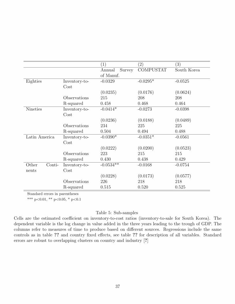
(1) (2) (3)Annual Surveyof Manuf.
COMPUSTAT South Korea
Eighties Inventory-to-Cost
-0.0329 -0.0295* -0.0525
(0.0235) (0.0176) (0.0624)Observations 215 208 208R-squared 0.458 0.468 0.464
Nineties Inventory-to-Cost
-0.0414* -0.0273 -0.0398
(0.0236) (0.0188) (0.0489)Observations 234 225 225R-squared 0.504 0.494 0.488
Latin America Inventory-to-Cost
-0.0390* -0.0351* -0.0561
(0.0222) (0.0200) (0.0523)Observations 223 215 215R-squared 0.430 0.438 0.429
Other Conti-nents
Inventory-to-Cost
-0.0534** -0.0168 -0.0754
(0.0228) (0.0173) (0.0577)Observations 226 218 218R-squared 0.515 0.520 0.525
Standard errors in parentheses*** p<0.01, ** p<0.05, * p<0.1
Table 5: Sub-samplesCells are the estimated coefficient on inventory-to-cost ratios (inventory-to-sale for South Korea). Thedependent variable is the log change in value added in the three years leading to the trough of GDP. Thecolumns refer to measures of time to produce based on different sources. Regressions include the samecontrols as in table ?? and country fixed effects, see table ?? for description of all variables. Standarderrors are robust to overlapping clusters on country and industry [?]
37

Annual Survey of Manuf. COMPUSTAT South Koreat*-3 to t* Inventory
Turnover-0.0404** -0.0307* -0.0519
(0.0177) (0.0157) (0.0408)Observations 449 433 433
t*-2 to t* InventoryTurnover
-.0241* -.0238** -.0351
(0.0140) (0.0119) (0.0332)Observations 445 429 429
t*-3 to t*+3 InventoryTurnover
-0.0297 -.0307** -0.0442
(0.0250) (0.0140) (0.0425)Observations 361 334 334
t*-3 to t*+5 InventoryTurnover
-.0324 -0.0486*** -0.0662
(0.0245) (0.0177) (0.0453)Observations 446 430 430
Standard errors in parentheses*** p<0.01, ** p<0.05, * p<0.1
Table 6: Sensitivity to time windowThe columns refer to measures of time to produce based on different sources. Regressions include the samecontrols as in table ?? and country fixed effects, see table ?? for description of all variables. Standarderrors are robust to overlapping clusters on country and industry [?]
38

−4 −3 −2 −1 0 1 2 3 4−0.6
−0.5
−0.4
−0.3
−0.2
−0.1
0
0.1
Years from trough
Ave
rage
log
devi
atio
n fr
om p
revi
ous
tren
d
GDPInvestment
Figure 3: Aggregate Investment and GDPAverages over the 21 crises of the log deviation from trend of aggregate Gross Fixed Capital Formationand GDP. Trend is based on a linear estimate using data from 9 to 3 years before the trough of GDP
0 2 4 6 8 10−0.4
−0.35
−0.3
−0.25
−0.2
−0.15
−0.1
−0.05
0
Quarters from crisis
Log(
I/GD
P),
diff
eren
ce fr
om s
tead
y st
ate
Figure 4: Investment to GDP ratio in quarterly dataAverages of log deviations from steady state level over 6 episodes for which quarterly data is available:Argentina (2001), Ecuador (1999), Korea (1998), Malaysia (1998), Mexico (1995), Turkey (1999)
39

Parameter Valueθ Elasticity of demand for exports 20ρ Elasticity of substitution between home sectors 2σ Relative risk aversion 2ψ Elasticity of labor supply 2.3β Discount rate 0.97% p.y.ζ Elasticity of investment to marginal q 0.9143δK Depreciation of capital 10% (per year)δH Depreciation of capital in Real Estate Sector 2.3% (per year)δD Depreciation of durables 13% (per year)ξ Elasticity of maintenance cost to utilization 0.5ηr Persistence of interest rate shock 0.9934 (per quarter)ηa Persistence of TFP shock 0.9011 (per quarter)r Steady state interest rate 8.49% (per year)
Table 7: Benchmark Calibration
40

0 5 10 15−0.1
−0.08
−0.06
−0.04
−0.02
0
Quarters
GD
P
Interest Rate Shock
0 5 10 15−0.14
−0.12
−0.1
−0.08
−0.06
−0.04
Quarters
GD
P
TFP Shock
0 5 10 15−0.5
−0.45
−0.4
−0.35
−0.3
Quarters
Inve
stm
ent
Interest Rate Shock
0 5 10 15−0.05
−0.045
−0.04
−0.035
−0.03
−0.025
−0.02
Quarters
Inve
stm
ent
TFP Shock
Full Model
No Time to Produce in Manufacturing
Figure 5: Effect of shocks to interest rate and TFP on GDP and fixed investment.The shocks to TFP and interest rate are equal to -0.254% and 8.71% (yearly) respectively. Calibration isthe benchmark, given in table ??.
41

1 1.5 2 2.5 3−0.15
−0.1
−0.05
0
0.05
0.1
0.15
0.2
0.25Interest Rate Shock
Val
ue A
dded
S.S. Inventory/Cost (months)
1 1.5 2 2.5 3−0.22
−0.2
−0.18
−0.16
−0.14
−0.12
−0.1Productivity Shock
Val
ue A
dded
S.S. Inventory/Cost (months)
Full ModelNo Time to Produce in Manufacturing
Figure 6: Cross-Sectional Reallocation Among Manufacturing Industries for Different ShocksLevel of output in different manufacturing industries in the year when aggregate GDP is at its trough.The shocks to TFP and interest rate are equal to -0.254% and 8.71% (yearly) respectively. Calibration isthe benchmark, given in table. Model generated data is time-aggregated from quarterly to yearly. Thenumber depicted in the graph are averages over all possible starting dates for the crisis, starting from thesecond quarter in t*-1 to the first quarter in t*, where t* is the year when GDP is at the trough. Data foreach industry are averages across episodes of the deviations from linear trends estimated for each seriesindividually based on data from t*-9 to t*-3
42

Model t* t*+3Benchmark value -0.017 -0.025
p-stat 18.6% 84.3%No Time to Produce in Manufacturing value 0.009 0.005
p-stat 0.6% 16.7%θ = 2 value 0.007 -0.006
p-stat 0.8% 33.8%θ = 200 value -0.085 -0.102
p-stat 1.3% 0.4%χ = 0.1 value -0.023 -0.036
p-stat 32.8% 80.9%χ = 1 value -0.012 -0.018
p-stat 11.0% 65.3%ψ = 4.54 value -0.015 -0.025
p-stat 15.2% 85.9%ψ = 1.13 value -0.018 -0.024
p-stat 19.6% 81%Data -0.040 -0.030
Table 8: Coefficients on Inventory-to-Cost ratios Coefficients on Inventory-to-Cost ratios measured inmonths when model generated data is regressed on inventory-to-cost and controls for demand side (in-vestment, export and durable consumption orientation) and supply side (share of wages, materials andimported goods in inputs) heterogeneity. Data is coefficients on full regressions (see table ??). p-statsare from a test that coefficient estimated in the data is equal to the coefficient calculated for the model.Remaining calibrated parameters are all as in table ??.
43
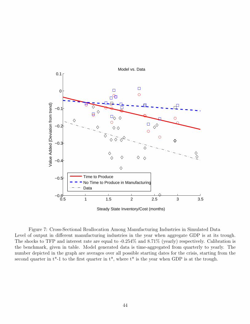
0.5 1 1.5 2 2.5 3 3.5−0.6
−0.5
−0.4
−0.3
−0.2
−0.1
0
0.1
Steady State Inventory/Cost (months)
Val
ue A
dded
(D
evia
tion
from
tren
d)
Model vs. Data
Time to ProduceNo Time to Produce in ManufacturingData
Figure 7: Cross-Sectional Reallocation Among Manufacturing Industries in Simulated DataLevel of output in different manufacturing industries in the year when aggregate GDP is at its trough.The shocks to TFP and interest rate are equal to -0.254% and 8.71% (yearly) respectively. Calibration isthe benchmark, given in table. Model generated data is time-aggregated from quarterly to yearly. Thenumber depicted in the graph are averages over all possible starting dates for the crisis, starting from thesecond quarter in t*-1 to the first quarter in t*, where t* is the year when GDP is at the trough.
44

−1.5 −1 −0.5 0 0.5 1 1.5−0.4
−0.3
−0.2
−0.1
0
0.1
0.2
0.3
Steady State Inventory/Cost (months)
Val
ue A
dded
(D
evia
tion
from
Ave
rage
)
Model vs. Data (same intercept)
Time to ProduceNo Time to Produce in ManufacturingData
Figure 8: Cross-Sectional Reallocation Among Manufacturing Industries in Simulated Data: Deviationsfrom MeansLevel of output in different manufacturing industries in the year when aggregate GDP is at its trough.The shocks to TFP and interest rate are equal to -0.254% and 8.71% (yearly) respectively. Calibration isthe benchmark, given in table. Model generated data is time-aggregated from quarterly to yearly. Thenumber depicted in the graph are averages over all possible starting dates for the crisis, starting from thesecond quarter in t*-1 to the first quarter in t*, where t* is the year when GDP is at the trough.
45
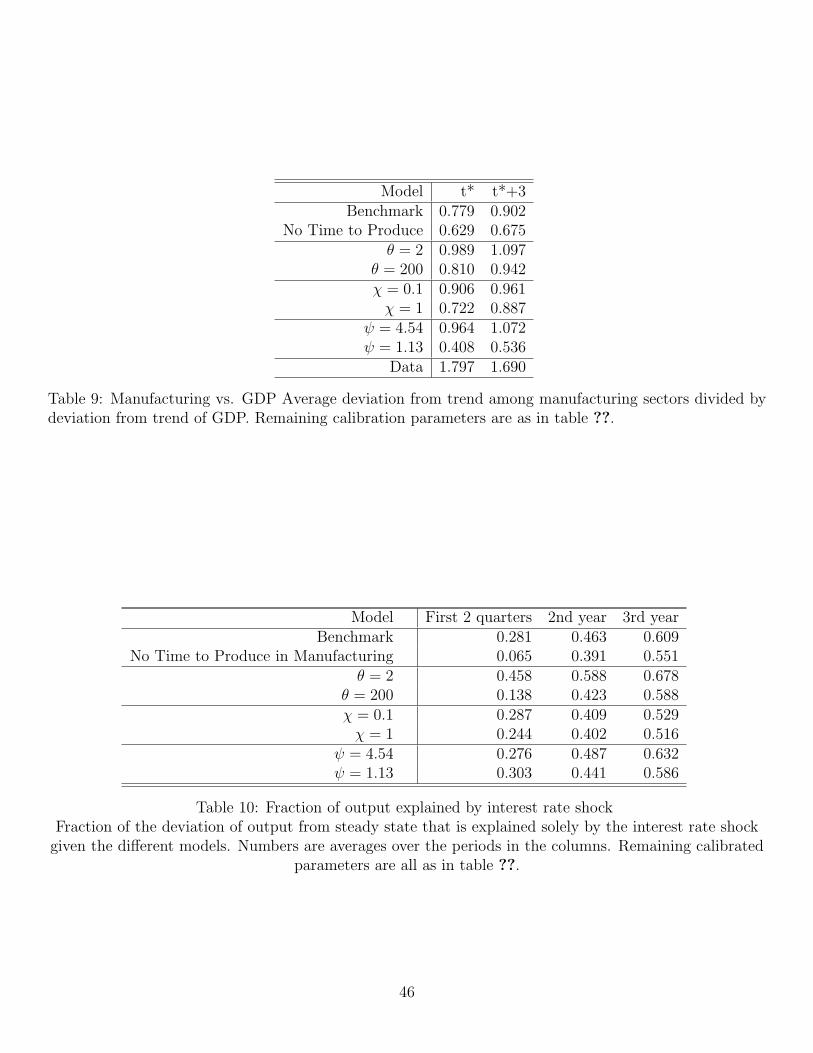
Model t* t*+3Benchmark 0.779 0.902
No Time to Produce 0.629 0.675θ = 2 0.989 1.097
θ = 200 0.810 0.942χ = 0.1 0.906 0.961χ = 1 0.722 0.887
ψ = 4.54 0.964 1.072ψ = 1.13 0.408 0.536
Data 1.797 1.690
Table 9: Manufacturing vs. GDP Average deviation from trend among manufacturing sectors divided bydeviation from trend of GDP. Remaining calibration parameters are as in table ??.
Model First 2 quarters 2nd year 3rd yearBenchmark 0.281 0.463 0.609
No Time to Produce in Manufacturing 0.065 0.391 0.551θ = 2 0.458 0.588 0.678
θ = 200 0.138 0.423 0.588χ = 0.1 0.287 0.409 0.529χ = 1 0.244 0.402 0.516
ψ = 4.54 0.276 0.487 0.632ψ = 1.13 0.303 0.441 0.586
Table 10: Fraction of output explained by interest rate shockFraction of the deviation of output from steady state that is explained solely by the interest rate shock
given the different models. Numbers are averages over the periods in the columns. Remaining calibratedparameters are all as in table ??.
46
Top Related