


Languages
Pages
Legal

This Week’s Topics Review Class Concepts
- AC/MC Rules of Overhead
- Simple Pricing
- Price Elasticity of Demand
Review Homework Practice Problems
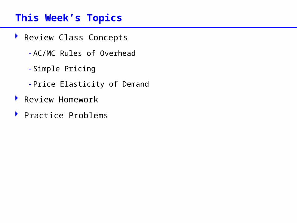
Class Concepts – AC/MC Rules of Overhead Sequential Decisions
- Should I produce the first product?
- Is the price I can sell at greater than average cost?
- Should I, also, produce the second product?
- Is the price I can sell at greater than marginal cost?
Knowledge Check: Which orders would I accept, if I received the following sequentially (not knowing I would receive the subsequent orders)?
- FC = 200, MC = 5
- Order 1: 100 units, Price = $6.50/unit
- Order 2: 200 units, Price = $6.01/unit
- Order 3: 50 units, Price = $5.50/unit
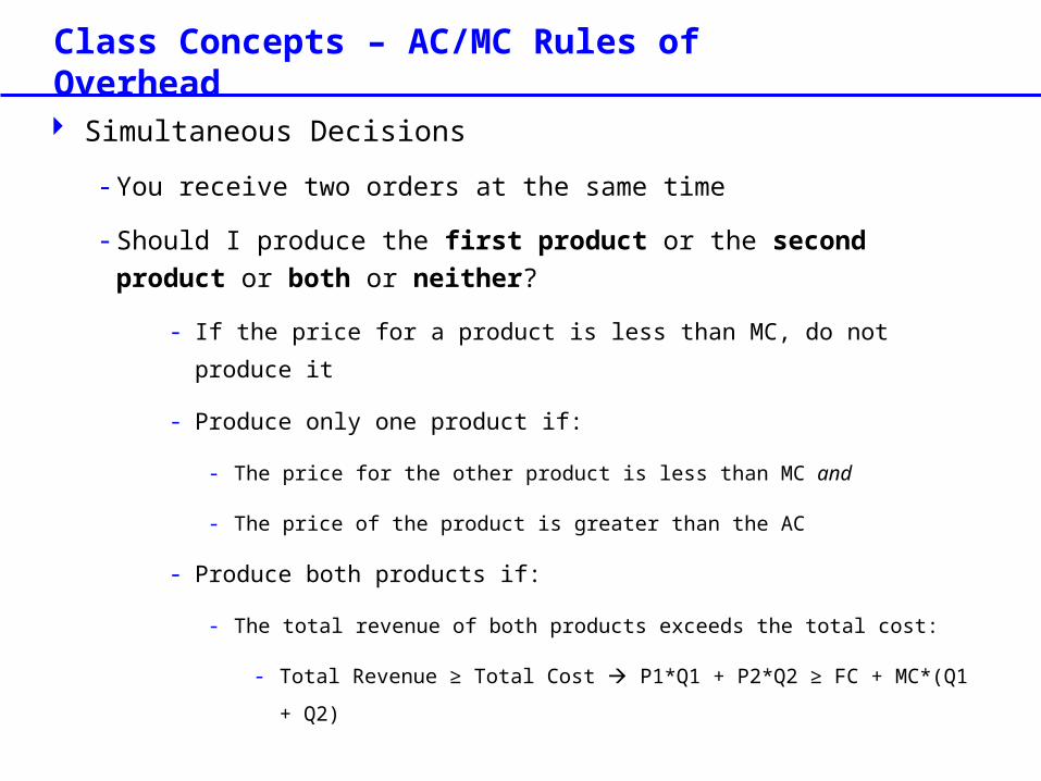
Class Concepts – AC/MC Rules of Overhead Simultaneous Decisions
- You receive two orders at the same time
- Should I produce the first product or the second product or both or neither?
- If the price for a product is less than MC, do not produce it
- Produce only one product if:
- The price for the other product is less than MC and
- The price of the product is greater than the AC
- Produce both products if:
- The total revenue of both products exceeds the total cost:
- Total Revenue ≥ Total Cost P1*Q1 + P2*Q2 ≥ FC + MC*(Q1 +
Q2)
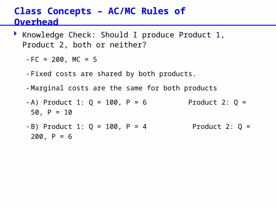
Class Concepts – AC/MC Rules of Overhead Knowledge Check: Should I produce Product 1, Product 2,
both or neither?
- FC = 200, MC = 5
- Fixed costs are shared by both products.
- Marginal costs are the same for both products
- A) Product 1: Q = 100, P = 6 Product 2: Q = 50, P = 10
- B) Product 1: Q = 100, P = 4 Product 2: Q = 200, P = 6
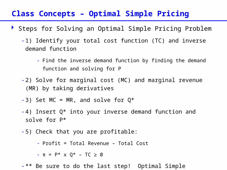
Class Concepts – Optimal Simple Pricing Steps for Solving an Optimal Simple Pricing Problem
- 1) Identify your total cost function (TC) and inverse demand function
- Find the inverse demand function by finding the demand function and solving for P
- 2) Solve for marginal cost (MC) and marginal revenue (MR) by taking derivatives
- 3) Set MC = MR, and solve for Q*
- 4) Insert Q* into your inverse demand function and solve for P*
- 5) Check that you are profitable:
- Profit = Total Revenue – Total Cost
- π = P* x Q* – TC ≥ 0
- ** Be sure to do the last step! Optimal Simple Pricing helps you figure out the most profit you can make from selling a good, given available demand. Is that optimal profit high enough to cover your fixed costs?
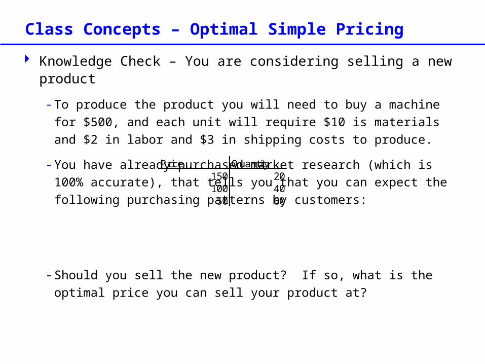
Class Concepts – Optimal Simple Pricing Knowledge Check – You are considering selling a new
product
- To produce the product you will need to buy a machine for $500, and each unit will require $10 is materials and $2 in labor and $3 in shipping costs to produce.
- You have already purchased market research (which is 100% accurate), that tells you that you can expect the following purchasing patterns by customers:
- Should you sell the new product? If so, what is the optimal price you can sell your product at?
Price Quantity150 20100 4050 60
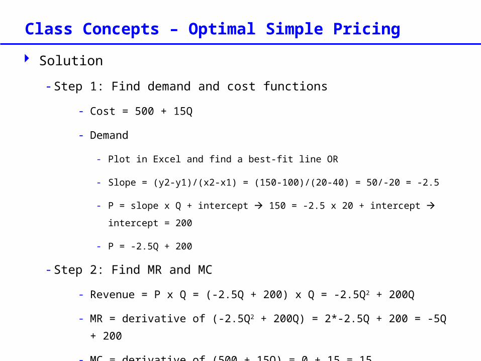
Class Concepts – Optimal Simple Pricing Solution
- Step 1: Find demand and cost functions
- Cost = 500 + 15Q
- Demand
- Plot in Excel and find a best-fit line OR
- Slope = (y2-y1)/(x2-x1) = (150-100)/(20-40) = 50/-20 = -2.5
- P = slope x Q + intercept 150 = -2.5 x 20 + intercept intercept =
200
- P = -2.5Q + 200
- Step 2: Find MR and MC
- Revenue = P x Q = (-2.5Q + 200) x Q = -2.5Q2 + 200Q
- MR = derivative of (-2.5Q2 + 200Q) = 2*-2.5Q + 200 = -5Q + 200
- MC = derivative of (500 + 15Q) = 0 + 15 = 15
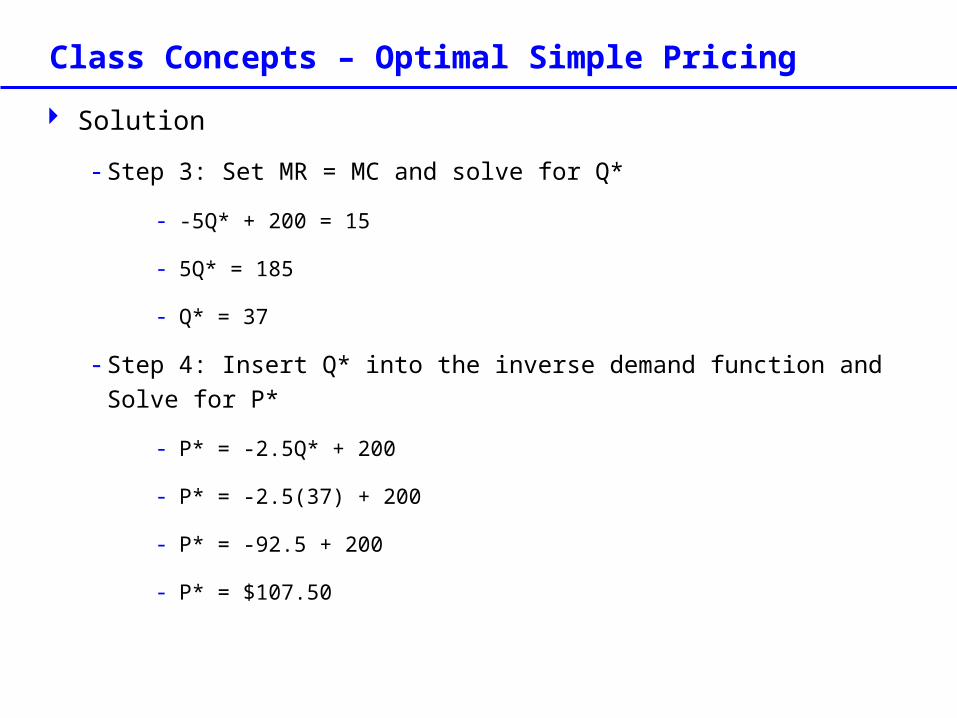
Class Concepts – Optimal Simple Pricing Solution
- Step 3: Set MR = MC and solve for Q*
- -5Q* + 200 = 15
- 5Q* = 185
- Q* = 37
- Step 4: Insert Q* into the inverse demand function and Solve for P*
- P* = -2.5Q* + 200
- P* = -2.5(37) + 200
- P* = -92.5 + 200
- P* = $107.50
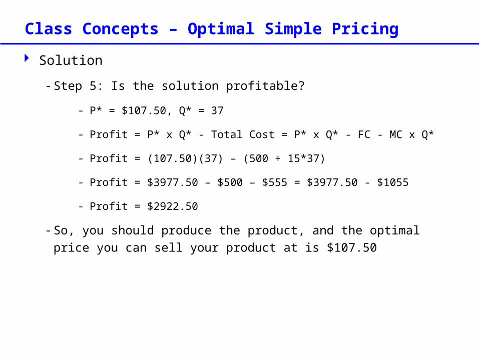
Class Concepts – Optimal Simple Pricing Solution
- Step 5: Is the solution profitable?
- P* = $107.50, Q* = 37
- Profit = P* x Q* - Total Cost = P* x Q* - FC - MC x Q*
- Profit = (107.50)(37) – (500 + 15*37)
- Profit = $3977.50 – $500 – $555 = $3977.50 - $1055
- Profit = $2922.50
- So, you should produce the product, and the optimal price you can sell your product at is $107.50
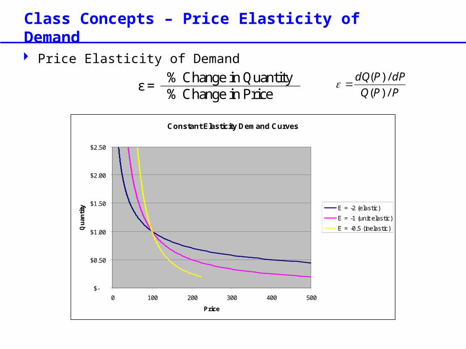
Class Concepts – Price Elasticity of Demand Price Elasticity of Demand
% Change in Quantity ε = % Change in Price
Constant Elasticity Demand Curves
$-
$0.50
$1.00
$1.50
$2.00
$2.50
0 100 200 300 400 500
Price
Qua
ntity E = -2 (elastic)
E = -1 (unit elastic)E = -0.5 (inelastic)
PPQdPPdQ
/)(/)(
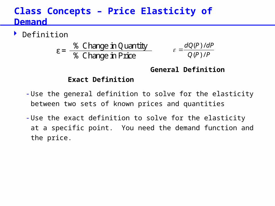
Class Concepts – Price Elasticity of Demand Definition
General Definition Exact Definition
- Use the general definition to solve for the elasticity between two sets of known prices and quantities
- Use the exact definition to solve for the elasticity at a specific point. You need the demand function and the price.
% Change in Quantity ε = % Change in Price
PPQdPPdQ
/)(/)(
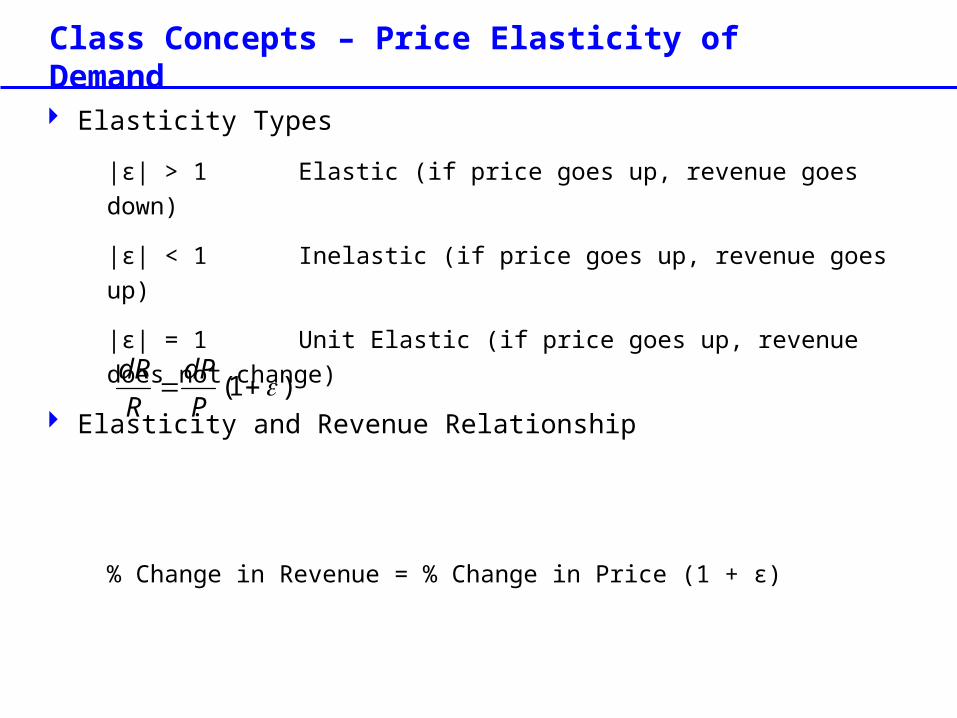
Class Concepts – Price Elasticity of Demand Elasticity Types
|ε| > 1 Elastic (if price goes up, revenue goes down)
|ε| < 1 Inelastic (if price goes up, revenue goes up)
|ε| = 1 Unit Elastic (if price goes up, revenue does not change)
Elasticity and Revenue Relationship
% Change in Revenue = % Change in Price (1 + ε)
)1( PdP
RdR
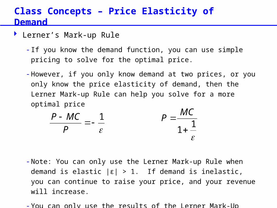
Class Concepts – Price Elasticity of Demand Lerner’s Mark-up Rule
- If you know the demand function, you can use simple pricing to solve for the optimal price.
- However, if you only know demand at two prices, or you only know the price elasticity of demand, then the Lerner Mark-up Rule can help you solve for a more optimal price
- Note: You can only use the Lerner Mark-up Rule when demand is elastic |ε| > 1. If demand is inelastic, you can continue to raise your price, and your revenue will increase.
- You can only use the results of the Lerner Mark-Up Rule if the resulting optimal price is close to your original known demand points
1
PMCP
11
MCP
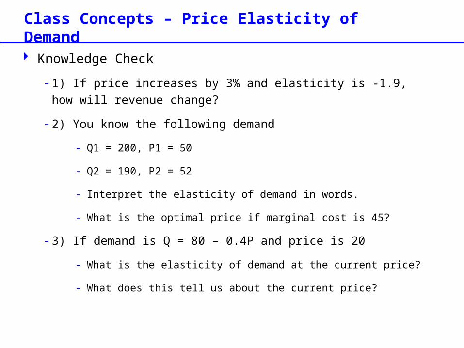
Class Concepts – Price Elasticity of Demand Knowledge Check
- 1) If price increases by 3% and elasticity is -1.9, how will revenue change?
- 2) You know the following demand
- Q1 = 200, P1 = 50
- Q2 = 190, P2 = 52
- Interpret the elasticity of demand in words.
- What is the optimal price if marginal cost is 45?
- 3) If demand is Q = 80 – 0.4P and price is 20
- What is the elasticity of demand at the current price?
- What does this tell us about the current price?
Class Concepts – Price Elasticity of Demand Knowledge Check
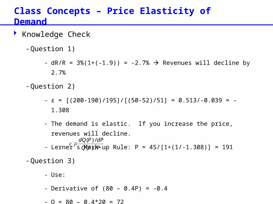
- Question 1)
- dR/R = 3%(1+(-1.9)) = -2.7% Revenues will decline by 2.7%
- Question 2)
- ε = [(200-190)/195]/[(50-52)/51] = 0.513/-0.039 = -1.308
- The demand is elastic. If you increase the price, revenues will decline.
- Lerner’s Mark-up Rule: P = 45/[1+(1/-1.308)] = 191
- Question 3)
- Use:
- Derivative of (80 – 0.4P) = -0.4
- Q = 80 – 0.4*20 = 72
- ε = -0.4/(72/20) = -0.4/3.6 = -0.111
PPQdPPdQ
/)(/)(
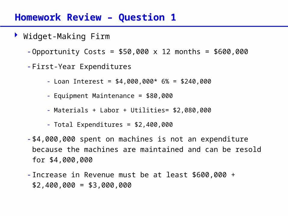
Homework Review – Question 1 Widget-Making Firm
- Opportunity Costs = $50,000 x 12 months = $600,000
- First-Year Expenditures
- Loan Interest = $4,000,000* 6% = $240,000
- Equipment Maintenance = $80,000
- Materials + Labor + Utilities= $2,080,000
- Total Expenditures = $2,400,000
- $4,000,000 spent on machines is not an expenditure because the machines are maintained and can be resold for $4,000,000
- Increase in Revenue must be at least $600,000 + $2,400,000 = $3,000,000
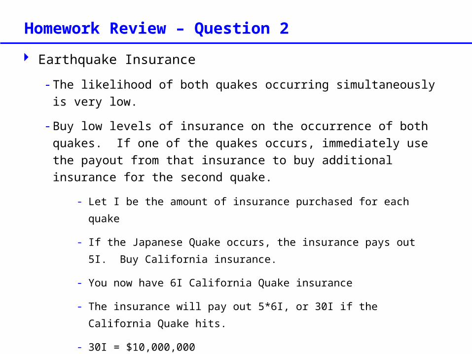
Homework Review – Question 2 Earthquake Insurance
- The likelihood of both quakes occurring simultaneously is very low.
- Buy low levels of insurance on the occurrence of both quakes. If one of the quakes occurs, immediately use the payout from that insurance to buy additional insurance for the second quake.
- Let I be the amount of insurance purchased for each quake
- If the Japanese Quake occurs, the insurance pays out 5I. Buy California insurance.
- You now have 6I California Quake insurance
- The insurance will pay out 5*6I, or 30I if the California Quake hits.
- 30I = $10,000,000
- I = 333,333.34
- So, the company should buy $333,333.34 in insurance on the Japanese Quake and buy $333,333.34 in insurance on the California Quake
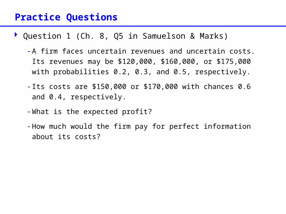
Practice Questions Question 1 (Ch. 8, Q5 in Samuelson & Marks)
- A firm faces uncertain revenues and uncertain costs. Its revenues may be $120,000, $160,000, or $175,000 with probabilities 0.2, 0.3, and 0.5, respectively.
- Its costs are $150,000 or $170,000 with chances 0.6 and 0.4, respectively.
- What is the expected profit?
- How much would the firm pay for perfect information about its costs?
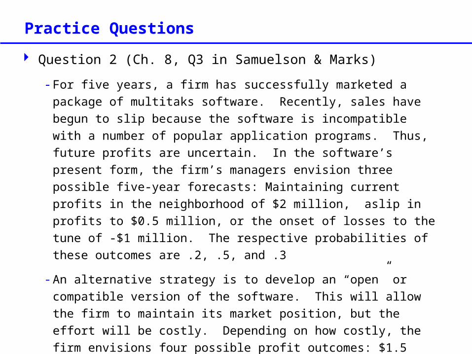
Practice Questions Question 2 (Ch. 8, Q3 in Samuelson & Marks)
- For five years, a firm has successfully marketed a package of multitaks software. Recently, sales have begun to slip because the software is incompatible with a number of popular application programs. Thus, future profits are uncertain. In the software’s present form, the firm’s managers envision three possible five-year forecasts: Maintaining current profits in the neighborhood of $2 million, aslip in profits to $0.5 million, or the onset of losses to the tune of -$1 million. The respective probabilities of these outcomes are .2, .5, and .3
- An alternative strategy is to develop an “open” or compatible version of the software. This will allow the firm to maintain its market position, but the effort will be costly. Depending on how costly, the firm envisions four possible profit outcomes: $1.5 million, $1.1 million, $0.8 million, and $0.6 million, with each outcome considered equally likely.
- Which course of action produces greater expected profit?
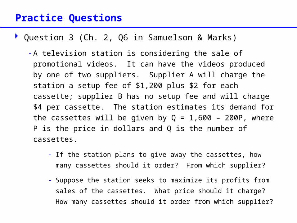
Practice Questions Question 3 (Ch. 2, Q6 in Samuelson & Marks)
- A television station is considering the sale of promotional videos. It can have the videos produced by one of two suppliers. Supplier A will charge the station a setup fee of $1,200 plus $2 for each cassette; supplier B has no setup fee and will charge $4 per cassette. The station estimates its demand for the cassettes will be given by Q = 1,600 – 200P, where P is the price in dollars and Q is the number of cassettes.
- If the station plans to give away the cassettes, how many cassettes should it order? From which supplier?
- Suppose the station seeks to maximize its profits from sales of the cassettes. What price should it charge? How many cassettes should it order from which supplier?
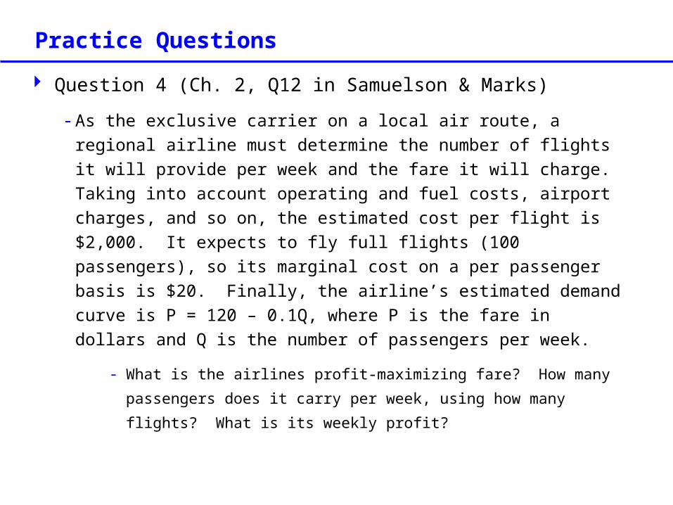
Practice Questions Question 4 (Ch. 2, Q12 in Samuelson & Marks)
- As the exclusive carrier on a local air route, a regional airline must determine the number of flights it will provide per week and the fare it will charge. Taking into account operating and fuel costs, airport charges, and so on, the estimated cost per flight is $2,000. It expects to fly full flights (100 passengers), so its marginal cost on a per passenger basis is $20. Finally, the airline’s estimated demand curve is P = 120 – 0.1Q, where P is the fare in dollars and Q is the number of passengers per week.
- What is the airlines profit-maximizing fare? How many passengers does it carry per week, using how many flights? What is its weekly profit?