


Languages
Pages
Legal

1
The uValue Companion: A Handbook on Valuation

2
CHAPTER 1
APPROACHES TO VALUATION In general terms, there are three approaches to valuation. The first, discounted
cashflow valuation, relates the value of an asset to the present value of expected future
cashflows on that asset. The second, relative valuation, estimates the value of an asset by
looking at the pricing of 'comparable' assets relative to a common variable like earnings,
cashflows, book value or sales. The third, contingent claim valuation, uses option pricing
models to measure the value of assets that share option characteristics.
Discounted Cashflow Valuation
In discounted cashflows valuation, the value of an asset is the present value of the
expected cashflows on the asset, discounted back at a rate that reflects the riskiness of
these cashflows. This approach gets the most play in classrooms and comes with the best
theoretical credentials.
Basis for Approach
We buy most assets because we expect them to generate cash flows for us in the
future. In discounted cash flow valuation, we begin with a simple proposition. The value
of an asset is not what someone perceives it to be worth but it is a function of the
expected cash flows on that asset. Put simply, assets with high and predictable cash flows
should have higher values than assets with low and volatile cash flows. In discounted
cash flow valuation, we estimate the value of an asset as the present value of the expected
cash flows on it.
€
Value of asset = E(CF1)(1+ r)
+E(CF2 )(1+ r)2 +
E(CF3 )(1+ r)3 ..... +
E(CFn )(1+ r)n
where,
n = Life of the asset
E(CFt) = Expected cashflow in period t
r = Discount rate reflecting the riskiness of the estimated cashflows
The cashflows will vary from asset to asset -- dividends for stocks, coupons (interest) and
the face value for bonds and after-tax cashflows for a business. The discount rate will be
3
a function of the riskiness of the estimated cashflows, with higher rates for riskier assets
and lower rates for safer ones.
Using discounted cash flow models is in some sense an act of faith. We believe
that every asset has an intrinsic value and we try to estimate that intrinsic value by
looking at an asset’s fundamentals. What is intrinsic value? Consider it the value that
would be attached to an asset by an all-knowing analyst with access to all information
available right now and a perfect valuation model. No such analyst exists, of course, but
we all aspire to be as close as we can to this perfect analyst. The problem lies in the fact
that none of us ever gets to see what the true intrinsic value of an asset is and we
therefore have no way of knowing whether our discounted cash flow valuations are close
to the mark or not.
Classifying Discounted Cash Flow Models
There are three distinct ways in which we can categorize discounted cash flow
models. In the first, we differentiate between valuing a business as a going concern as
opposed to a collection of assets. In the second, we draw a distinction between valuing
the equity in a business and valuing the business itself. In the third, we lay out three
different and equivalent ways of doing discounted cash flow valuation – the expected
cash flow approach, a value based upon excess returns and adjusted present value.
a. Going Concern versus Asset Valuation
The value of an asset in the discounted cash flow framework is the present value
of the expected cash flows on that asset. Extending this proposition to valuing a business,
it can be argued that the value of a business is the sum of the values of the individual
assets owned by the business. While this may be technically right, there is a key
difference between valuing a collection of assets and a business. A business or a
company is an on-going entity with assets that it already owns and assets it expects to
invest in the future. This can be best seen when we look at the financial balance sheet (as
opposed to an accounting balance sheet) for an ongoing company in figure 1.1:

4
Note that investments that have already been made are categorized as assets in place, but
investments that we expect the business to make in the future are growth assets.
A financial balance sheet provides a good framework to draw out the differences
between valuing a business as a going concern and valuing it as a collection of assets. In
a going concern valuation, we have to make our best judgments not only on existing
investments but also on expected future investments and their profitability. While this
may seem to be foolhardy, a large proportion of the market value of growth companies
comes from their growth assets. In an asset-based valuation, we focus primarily on the
assets in place and estimate the value of each asset separately. Adding the asset values
together yields the value of the business. For companies with lucrative growth
opportunities, asset-based valuations will yield lower values than going concern
valuations.
One special case of asset-based valuation is liquidation valuation, where we value
assets based upon the presumption that they have to be sold now. In theory, this should be
equal to the value obtained from discounted cash flow valuations of individual assets but
the urgency associated with liquidating assets quickly may result in a discount on the
value. How large the discount will be will depend upon the number of potential buyers
for the assets, the asset characteristics and the state of the economy.
b. Equity Valuation versus Firm Valuation
There are two ways in which we can approach discounted cash flow valuation.
The first is to value the entire business, with both assets-in-place and growth assets; this
is often termed firm or enterprise valuation.
Assets Liabilities
Investments alreadymade
Debt
Equity
Borrowed money
Owner’s fundsInvestments yet tobe made
Assets in PlaceExisting InvestmentsGenerate cashflows today
Growth AssetsExpected Value that will be created by future investments
Figure 1.1: A Simple View of a Firm

5
The cash flows before debt payments and after reinvestment needs are called free cash
flows to the firm, and the discount rate that reflects the composite cost of financing from
all sources of capital is called the cost of capital.
The second way is to just value the equity stake in the business, and this is called
equity valuation.
The cash flows after debt payments and reinvestment needs are called free cash flows to
equity, and the discount rate that reflects just the cost of equity financing is the cost of
equity.
Note also that we can always get from the former (firm value) to the latter (equity
value) by netting out the value of all non-equity claims from firm value. Done right, the
value of equity should be the same whether it is valued directly (by discounting cash
Assets Liabilities
Assets in Place Debt
Equity
Discount rate reflects the cost of raising both debt and equity financing, in proportion to their use
Growth Assets
Firm Valuation
Cash flows considered are cashflows from assets, prior to any debt paymentsbut after firm has reinvested to create growth assets
Present value is value of the entire firm, and reflects the value of all claims on the firm.
Assets Liabilities
Assets in Place Debt
EquityDiscount rate reflects only the cost of raising equity financingGrowth Assets
Equity Valuation
Cash flows considered are cashflows from assets, after debt payments and after making reinvestments needed for future growth
Present value is value of just the equity claims on the firm
6
flows to equity a the cost of equity) or indirectly (by valuing the firm and subtracting out
the value of all non-equity claims).
c. Variations on DCF Models
The model that we have presented in this section, where expected cash flows are
discounted back at a risk-adjusted discount rate, is the most commonly used discounted
cash flow approach but there are two widely used variants. In the first, we separate the
cash flows into excess return cash flows and normal return cash flows. Earning the risk-
adjusted required return (cost of capital or equity) is considered a normal return cash flow
but any cash flows above or below this number are categorized as excess returns; excess
returns can therefore be either positive or negative. With the excess return valuation
framework, the value of a business can be written as the sum of two components:
Value of business = Capital Invested in firm today + Present value of excess
return cash flows from both existing and future projects
If we make the assumption that the accounting measure of capital invested (book value of
capital) is a good measure of capital invested in assets today, this approach implies that
firms that earn positive excess return cash flows will trade at market values higher than
their book values and that the reverse will be true for firms that earn negative excess
return cash flows.
In the second variation, called the adjusted present value (APV) approach, we
separate the effects on value of debt financing from the value of the assets of a business.
In general, using debt to fund a firm’s operations creates tax benefits (because interest
expenses are tax deductible) on the plus side and increases bankruptcy risk (and expected
bankruptcy costs) on the minus side. In the APV approach, the value of a firm can be
written as follows:
Value of business = Value of business with 100% equity financing + Present
value of Expected Tax Benefits of Debt – Expected Bankruptcy Costs
In contrast to the conventional approach, where the effects of debt financing are captured
in the discount rate, the APV approach attempts to estimate the expected dollar value of
debt benefits and costs separately from the value of the operating assets.

7
While proponents of each approach like to claim that their approach is the best
and most precise, we will show later in the book that the three approaches yield the same
estimates of value, if we make consistent assumptions.
Inputs to Discounted Cash Flow Models
There are three inputs that are required to value any asset in this model - the
expected cash flow, the timing of the cash flow and the discount rate that is appropriate
given the riskiness of these cash flows.
a. Discount Rates
In valuation, we begin with the fundamental notion that the discount rate used on
a cash flow should reflect its riskiness, with higher risk cash flows having higher discount
rates. There are two ways of viewing risk. The first is purely in terms of the likelihood
that an entity will default on a commitment to make a payment, such as interest or
principal due, and this is called default risk. When looking at debt, the cost of debt is the
rate that reflects this default risk.
The second way of viewing risk is in terms of the variation of actual returns
around expected returns. The actual returns on a risky investment can be very different
from expected returns; the greater the variation, the greater the risk. When looking at
equity, we tend to use measures of risk based upon return variance. There are some basic
points on which these models agree. The first is that risk in an investment has to
perceived through the eyes of the marginal investor in that investment, and this marginal
investor is assumed to be well diversified across multiple investments. Therefore, the risk
in an investment that should determine discount rates is the non-diversifiable or market
risk of that investment. The second is that the expected return on any investment can be
obtained starting with the expected return on a riskless investment, and adding to it a
premium to reflect the amount of market risk in that investment. This expected return
yields the cost of equity.
The cost of capital can be obtained by taking an average of the cost of equity,
estimated as above, and the after-tax cost of borrowing, based upon default risk, and
weighting by the proportions used by each. We will argue that the weights used, when
valuing an on-going business, should be based upon the market values of debt and equity.

8
While there are some analysts who use book value weights, doing so violates a basic
principle of valuation, which is that at a fair value1, one should be indifferent between
buying and selling an asset.
b. Expected Cash Flows
In the strictest sense, the only cash flow an equity investor gets out of a publicly
traded firm is the dividend; models that use the dividends as cash flows are called
dividend discount models. A broader definition of cash flows to equity would be the cash
flows left over after the cash flow claims of non-equity investors in the firm have been
met (interest and principal payments to debt holders and preferred dividends) and after
enough of these cash flows has been reinvested into the firm to sustain the projected
growth in cash flows. This is the free cash flow to equity (FCFE), and models that use
these cash flows are called FCFE discount models.
The cashflow to the firm is the cumulated cash flow to all claimholders in the
firm. One way to obtain this cashflow is to add the free cash flows to equity to the cash
flows to lenders (debt) and preferred stockholders. A far simpler way of obtaining the
same number is to estimate the cash flows prior to debt and preferred dividend payments,
by subtracting from the after-tax operating income the net investment needs to sustain
growth. This cash flow is called the free cash flow to the firm (FCFF) and the models that
use these cash flows are called FCFF models.
c. Expected Growth
It is while estimating the expected growth in cash flows in the future that analysts
confront uncertainty most directly. There are three generic ways of estimating growth.
One is to look at a company’s past and use the historical growth rate posted by that
company. The peril is that past growth may provide little indication of future growth. The
second is to obtain estimates of growth from more informed sources. For some analysts, 1 When book value weights are used, the costs of capital tend to be much lower for many U.S. firms, since
book equity is lower than market equity. This then pushes up the value for these firms. While this may
make it attractive to the sellers of these firms, very few buyers would be willing to pay this price for the
firm, since it would require that the debt that they use in their financing will have to be based upon the
book value, often requiring tripling or quadrupling the dollar debt in the firm.

9
this translates into using the estimates provided by a company’s management whereas for
others it takes the form of using consensus estimates of growth made by others who
follow the firm. The bias associated with both these sources should raise questions about
the resulting valuations.
There is a third way to estimate growth, where the expected growth rate is tied to
two variables that are determined by the firm being valued - how much of the earnings
are reinvested back into the firm and how well those earnings are reinvested. In the equity
valuation model, this expected growth rate is a product of the retention ratio, i.e. the
proportion of net income not paid out to stockholders, and the return on equity on the
projects taken with that money. In the firm valuation model, the expected growth rate is a
product of the reinvestment rate, which is the proportion of after-tax operating income
that goes into net new investments and the return on capital earned on these investments.
The advantages of using these fundamental growth rates are two fold. The first is that the
resulting valuations will be internally consistent and companies that are assumed to have
high growth are required to pay for the growth with more reinvestment. The second is
that it lays the foundation for considering how firms can make themselves more valuable
to their investors.
DCF Valuation: Pluses and Minuses
To true believers, discounted cash flow valuation is the only way to approach
valuation, but the benefits may be more nuanced that they are willing to admit. On the
plus side, discounted cash flow valuation, done right, requires analysts to understand the
businesses that they are valuing and ask searching questions about the sustainability of
cash flows and risk. Discounted cash flow valuation is tailor made for those who buy into
the Warren Buffett adage that what we are buying are not stocks but the underlying
businesses. In addition, discounted cash flow valuations is inherently contrarian in the
sense that it forces analysts to look for the fundamentals that drive value rather than what
market perceptions are. Consequently, if stock prices rise (fall) disproportionately relative
to the underlying earnings and cash flows, discounted cash flows models are likely to
find stocks to be over valued (under valued).

10
There are, however, limitations with discounted cash flow valuation. In the hands
of sloppy analysts, discounted cash flow valuations can be manipulated to generate
estimates of value that have no relationship to intrinsic value. We also need substantially
more information to value a company with discounted cash flow models, since we have
to estimate cashflows, growth rates and discount rates. Finally, discounted cash flow
models may very well find every stock in a sector or even a market to be over valued, if
market perceptions have run ahead of fundamentals. For portfolio managers and equity
research analysts, who are required to find equities to buy even in the most over valued
markets, this creates a conundrum. They can go with their discounted cash flow
valuations and conclude that everything is overvalued, which may put them out of
business, or they can find an alternate approach that is more sensitive to market moods. It
should come as no surprise that many choose the latter.
Relative Valuation While the focus in classrooms and academic discussions remains on discounted
cash flow valuation, the reality is that most assets are valued on a relative basis. In
relative valuation, we value an asset by looking at how the market prices similar assets.
Thus, when determining what to pay for a house, we look at what similar houses in the
neighborhood sold for rather than doing an intrinsic valuation. Extending this analogy to
stocks, investors often decide whether a stock is cheap or expensive by comparing its
pricing to that of similar stocks (usually in its peer group). In this section, we will
consider the basis for relative valuation, ways in which it can be used and its advantages
and disadvantages.
Basis for approach
In relative valuation, the value of an asset is derived from the pricing of
'comparable' assets, standardized using a common variable. Included in this description
are two key components of relative valuation. The first is the notion of comparable or
similar assets. From a valuation standpoint, this would imply assets with similar cash
flows, risk and growth potential. In practice, it is usually taken to mean other companies
that are in the same business as the company being valued. The other is a standardized
price. After all, the price per share of a company is in some sense arbitrary since it is a

11
function of the number of shares outstanding; a two for one stock split would halve the
price. Dividing the price or market value by some measure that is related to that value
will yield a standardized price. When valuing stocks, this essentially translates into using
multiples where we divide the market value by earnings, book value or revenues to arrive
at an estimate of standardized value. We can then compare these numbers across
companies.
The simplest and most direct applications of relative valuations are with real
assets where it is easy to find similar assets or even identical ones. The asking price for a
Mickey Mantle rookie baseball card or a 1965 Ford Mustang is relatively easy to estimate
given that there are other Mickey Mantle cards and 1965 Ford Mustangs out there and
that the prices at which they have been bought and sold can be obtained. With equity
valuation, relative valuation becomes more complicated by two realities. The first is the
absence of similar assets, requiring us to stretch the definition of comparable to include
companies that are different from the one that we are valuing. After all, what company in
the world is remotely similar to Microsoft or GE? The other is that different ways of
standardizing prices (different multiples) can yield different values for the same
company.
Harking back to our earlier discussion of discounted cash flow valuation, we
argued that discounted cash flow valuation was a search (albeit unfulfilled) for intrinsic
value. In relative valuation, we have given up on estimating intrinsic value and
essentially put our trust in markets getting it right, at least on average.
Variations on Relative Valuation
In relative valuation, the value of an asset is based upon how similar assets are
priced. In practice, there are three variations on relative valuation, with the differences
primarily in how we define comparable firms and control for differences across firms:
a. Direct comparison: In this approach, analysts try to find one or two companies that
look almost exactly like the company they are trying to value and estimate the value
based upon how these “similar” companies are priced. The key part in this analysis is
identifying these similar companies and getting their market values.

12
b. Peer Group Average: In the second, analysts compare how their company is priced
(using a multiple) with how the peer group is priced (using the average for that multiple).
Thus, a stock is considered cheap if it trade at 12 times earnings and the average price
earnings ratio for the sector is 15. Implicit in this approach is the assumption that while
companies may vary widely across a sector, the average for the sector is representative
for a typical company.
c. Peer group average adjusted for differences: Recognizing that there can be wide
differences between the company being valued and other companies in the comparable
firm group, analysts sometimes try to control for differences between companies. In
many cases, the control is subjective: a company with higher expected growth than the
industry will trade at a higher multiple of earnings than the industry average but how
much higher is left unspecified. In a few cases, analysts explicitly try to control for
differences between companies by either adjusting the multiple being used or by using
statistical techniques. As an example of the former, consider PEG ratios. These ratios are
computed by dividing PE ratios by expected growth rates, thus controlling (at least in
theory) for differences in growth and allowing analysts to compare companies with
different growth rates. For statistical controls, we can use a multiple regression where we
can regress the multiple that we are using against the fundamentals that we believe cause
that multiple to vary across companies. The resulting regression can be used to estimate
the value of an individual company. In fact, we will argue later in this book that statistical
techniques are powerful enough to allow us to expand the comparable firm sample to
include the entire market.
Applicability of multiples and limitations
The allure of multiples is that they are simple and easy to relate to. They can be
used to obtain estimates of value quickly for firms and assets, and are particularly useful
when there are a large number of comparable firms being traded on financial markets,
and the market is, on average, pricing these firms correctly. In fact, relative valuation is
tailor made for analysts and portfolio managers who not only have to find under valued
equities in any market, no matter how overvalued, but also get judged on a relative basis.
An analyst who picks stocks based upon their PE ratios, relative to the sectors they

13
operate in, will always find under valued stocks in any market; if entire sectors are over
valued and his stocks decline, he will still look good on a relative basis since his stocks
will decline less than comparable stocks (assuming the relative valuation is right).
By the same token, they are also easy to misuse and manipulate, especially when
comparable firms are used. Given that no two firms are exactly similar in terms of risk
and growth, the definition of 'comparable' firms is a subjective one. Consequently, a
biased analyst can choose a group of comparable firms to confirm his or her biases about
a firm's value. While this potential for bias exists with discounted cashflow valuation as
well, the analyst in DCF valuation is forced to be much more explicit about the
assumptions which determine the final value. With multiples, these assumptions are often
left unstated.
The other problem with using multiples based upon comparable firms is that it
builds in errors (over valuation or under valuation) that the market might be making in
valuing these firms. If, for instance, we find a company to be under valued because it
trades at 15 times earnings and comparable companies trade at 25 times earnings, we may
still lose on the investment if the entire sector is over valued. In relative valuation, all that
we can claim is that a stock looks cheap or expensive relative to the group we compared
it to, rather than make an absolute judgment about value. Ultimately, relative valuation
judgments depend upon how well we have picked the comparable companies and how
how good a job the market has done in pricing them.
Contingent Claim Valuation
There is little in either discounted cashflow or relative valuation that can be
considered new and revolutionary. In recent years, though, analysts have increasingly
used option-pricing models, developed to value listed options, to value assets, businesses
and equity stakes in businesses. These applications are often categorized loosely as real
options, but as we will see later in this book, they have to be used with caution.
Basis for Approach
A contingent claim or option is an asset which pays off only under certain
contingencies - if the value of the underlying asset exceeds a pre-specified value for a call
option, or is less than a pre-specified value for a put option. Much work has been done in

14
the last few decades in developing models that value options, and these option-pricing
models can be used to value any assets that have option-like features.
Figure 1.2 illustrates the payoffs on call and put options as a function of the value
of the underlying asset:
Figure 1.2: Payoffs on Options as a Function of the Underlying Asset's Value
An option can be valued as a function of the following variables - the current value and
the variance in value of the underlying asset, the strike price and the time to expiration of
the option and the riskless interest rate. This was first established by Black and Scholes
(1972) and has been extended and refined subsequently in numerous variants.2 While the
Black-Scholes option-pricing model ignored dividends and assumed that options would
not be exercised early, it can be modified to allow for both. A discrete-time variant, the
Binomial option-pricing model, has also been developed to price options.
An asset can be valued as a call option if the payoffs on it are a function of the
value of an underlying asset; if that value exceeds a pre-specified level, the asset is worth
the difference; if not, it is worth nothing. It can be valued as a put option if it gains value
as the value of the underlying asset drops below a pre- specified level, and if it is worth
2 Black, F. and M. Scholes, 1972, The Valuation of Option Contracts and a Test of Market Efficiency,
Journal of Finance, v27, 399-417.
Value of AssetStrike Price
Call OptionPut Option

15
nothing when the underlying asset's value exceeds that specified level. There are many
assets that generally are not viewed as options but still share several option
characteristics. A patent can be analyzed as a call option on a product, with the
investment outlay needed to get the project going considered the strike price and the
patent life becoming the life of the option. An undeveloped oil reserve or gold mine
provides its owner with a call option to develop the reserve or mine, if oil or gold prices
increase.
The essence of the real options argument is that discounted cash flow models
understate the value of assets with option characteristics. The understatement occurs
because DCF models value assets based upon a set of expected cash flows and do not
fully consider the possibility that firms can learn from real time developments and
respond to that learning. For example, an oil company can observe what the oil price is
each year and adjust its development of new reserves and production in existing reserves
accordingly rather than be locked into a fixed production schedule. As a result, there
should be an option premium added on to the discounted cash flow value of the oil
reserves. It is this premium on value that makes real options so alluring and so potentially
dangerous.
Applicability and Limitations
Using option-pricing models in valuation does have its advantages. First, there are
some assets that cannot be valued with conventional valuation models because their value
derives almost entirely from their option characteristics. For example, a biotechnology
firm with a single promising patent for a blockbuster cancer drug wending its way
through the FDA approval process cannot be easily valued using discounted cash flow or
relative valuation models. It can, however, be valued as an option. The same can be said
about equity in a money losing company with substantial debt; most investors buying this
stock are buying it for the same reasons they buy deep out-of-the-money options. Second,
option-pricing models do yield more realistic estimates of value for assets where there is
a significant benefit obtained from learning and flexibility. Discounted cash flow models
will understate the values of natural resource companies, where the observed price of the
natural resource is a key factor in decision making. Third, option-pricing models do

16
highlight a very important aspect of risk. While risk is considered almost always in
negative terms in discounted cash flow and relative valuation (with higher risk reducing
value), the value of options increases as volatility increases. For some assets, at least, risk
can be an ally and can be exploited to generate additional value.
This is not to suggest that using real options models is an unalloyed good. Using
real options arguments to justify paying premiums on discounted cash flow valuations,
when the options argument does not hold, can result in overpayment. While we do not
disagree with the notion that firms can learn by observing what happens over time, this
learning has value only if it has some degree of exclusivity. We will argue later in this
book that it is usually inappropriate to attach an option premium to value if the learning is
not exclusive and competitors can adapt their behavior as well. There are also limitations
in using option pricing models to value long-term options on non-traded assets. The
assumptions made about constant variance and dividend yields, which are not seriously
contested for short term options, are much more difficult to defend when options have
long lifetimes. When the underlying asset is not traded, the inputs for the value of the
underlying asset and the variance in that value cannot be extracted from financial markets
and have to be estimated. Thus the final values obtained from these applications of option
pricing models have much more estimation error associated with them than the values
obtained in their more standard applications (to value short term traded options).

17
CHAPTER 2
VALUING BUSINESSES ACROSS SECTORS AND THE LIFE CYCLE While the fundamentals of valuation are straightforward, the challenges we face
in valuing companies shift as these firms move through the life cycle from idea
businesses, often privately owned, to young growth companies, either public or on the
verge of going public, to mature companies, with diverse product lines and serving
different markets, to companies in decline, marking time until they are liquidated. At
each stage, we are called upon to estimate the same inputs – cash flows, growth rates and
discount rates – but with varying amounts of information and different degrees of
precision. All too often, when confronted with significant uncertainty or limited
information, we will be tempted by the dark side of valuation, where first principles are
abandoned, new paradigms are created and common sense is the casualty.
Foundations of Value Without delving into the estimation details, we can use the intrinsic value
equation of the business to list the four broad questions that we need to answer, in order
to value any business: What are the cash flows that will be generated by the existing
investments of the company? How much value, if any, will be added by future growth?
How risky are the expected cashflows from both existing and growth investments and
what is the cost of funding them? When will the firm become a stable growth firm,
allowing us to estimate a terminal value?
What are the cash flows generated by existing assets?
If a firm has significant investments that it has already made, the first inputs into
valuation are the cash flows from these existing assets. In practical terms, this requires
estimating how much the firm generated in earnings and cashflows from these assets in
the most recent period, how much growth (if any) is expected in these earnings/cashflows
over time and how long the assets will continue to generate cash flows. While data that
allows us to answer all of these questions may be available in current financial
statements, they might not be conclusive. In particular, cash flows can be difficult to
obtain if the existing assets are still not fully operational (infrastructure investments that

18
have been made, but are not in full production mode) or if they are not being efficiently
utilized. There can also be estimation issues when the firm in question is in a volatile
business, where earnings on existing assets can rise and fall as a result of macroeconomic
forces.
How much value will be added by future investments (growth)?
For some companies, the bulk of value will be derived from investments that you
expect them to make in the future. To estimate the value added by these investments, you
have to make judgments on two variables. The first is the magnitude of these new
investments, relative to the size of the firm. In other words, the value added can be very
different, if you assume that a firm reinvests 80% of its earnings back into new
investments than if you assume that it reinvests 20%. The second is the quality of the new
investments, measured in terms of excess returns, i.e., the returns the firm makes on the
investments over and above the cost of funding those investments. Investing in new
assets that generate returns of 15%, when the cost of capital of 10%, will add value, but
investing in new assets that generate returns of 10%, with the same cost of capital, will
not. In other, words, it is growth with excess returns that creates value, not growth per se.
Since growth assets rest entirely on expectations and perception, we can make
two statements about them. One is that valuing growth assets will generally pose more
challenges than valuing existing assets; historical or financial statement information is
less likely to provide conclusive results. The other is that there will be there will be far
more volatility in the value of growth assets than in the value of existing assets, both over
time and across different people valuing the same firm. Analysts are likely to not only
differ more on the inputs into growth asset value – the magnitude and quality of new
investments – but will also change their own estimates more over time, as new
information comes out about the firm. A poor earnings announcement by a growth
company may alter the value of its existing assets just a little but can dramatically shift
expectations about the value of growth assets.
How risky are the cashflows and what are the consequences for discount rates?
Neither the cash flows from existing assets, nor the cash flows from growth
investments, is guaranteed. When valuing these cash flows, we have to consider risk

19
somewhere and the discount rate is usually the vehicle that we use to convey the concerns
that we may have about uncertainty in the future. In practical terms, we use higher
discount rates to discount riskier cash flows, and thus give them a lower value than more
predictable cash flows. While this a common sense notion, there are issues that we run
into in putting this into practice, when valuing firms:
1. Dependence on the past: The risk that we are concerned about is entirely in the
future, but our estimates of risk are usually based upon data from the past –
historical prices, earnings and cash flows. While this dependence upon historical
data is understandable, it can give rise to problems when that data is unavailable,
unreliable or shifting.
2. Diverse risk investments: When valuing firms, we generally estimate one discount
rate for its aggregate cash flows, partly because of the way we estimate risk
parameters and partly for convenience. Firms do generate cashflows from
multiple assets, in different locations, with varying amounts of risk, and the
discount rates we use should be different for each set of cash flows.
3. Changes in risk over time: In most valuations, we estimate one discount rate and
we leave it unchanged over time, again partly for ease and partly because we feel
uncomfortable changing discount rates over time. When valuing a firm, though, it
is entirely possible, and indeed likely, that the risk of the firm will change over
time as its asset mix changes and it matures. In fact, if we accept the earlier
proposition that the cash flows from growth assets are more difficult to predict
than cash flows from existing assets, we should expect the discount rate used on
the cumulative expected cash flows of a growth firm to decrease as its growth rate
declines over time.
When will the firm become mature?
The question of when a firm will become a mature firm is relevant because it
determines the length of the high growth period and the value that we attach to the firm at
the end of the period (the terminal value). It is question that may be easy to answer for a
few firms, including larger and more stable firms that are either already mature
businesses or close to it, or firms that derive their growth from a single competitive
20
advantage with an expiration date (for instance, a patent). For most firms, the conclusion
will be murky for two reasons:
1. Making a judgment about when a firm will become mature requires us to look at
the sector in which the firm operates, the state of its competitors and what they
will do in the future. For firms in sectors that are evolving, with new entrants and
existing competitors exiting, this will be difficult to do.
2. While we are sanguine about mapping out pathways to the terminal value in
discounted cash flow models and generally assume that every firm makes it to
stable growth and goes on, the real world delivers surprises along the way that
may impede these paths. After all, most firms do not make it to the steady state
that we aspire, and instead get acquired, restructured or go bankrupt well before
the terminal year.
In summary, not only is estimating when a firm will become mature difficult to do, but
considering whether a firm will make it as a going concern for a valuation is just as
important.
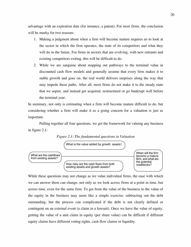
Pulling together all four questions, we get the framework for valuing any business
in figure 2.1:
Figure 2.1: The fundamental questions in Valuation
While these questions may not change as we value individual firms, the ease with which
we can answer them can change, not only as we look across firms at a point in time, but
across time, even for the same firm. To get from the value of the business to the value of
the equity in the business may seem like a simple exercise: subtracting out the debt
outstanding, but the process can complicated if the debt is not clearly defined or
contingent on an external event (a claim in a lawsuit). Once we have the value of equity,
getting the value of a unit claim in equity (per share value) can be difficult if different
equity claims have different voting rights, cash flow claims or liquidity.
What are the cashflows from existing assets?
What is the value added by growth assets?
How risky are the cash flows from both existing assets and growth assets?
When will the firm become a mature fiirm, and what are the potential roadblocks?

21
Valuation across the Life Cycle While the inputs into valuation are the same for all businesses, the challenges we
face in making the estimates can vary significantly across firms. In this section, we first
break firms down into four groups based upon where they are in the life cycle and then
explore the estimation issues we run into with firms in each stage.
The Business Life Cycle Firms pass through a life cycle, starting as young, idea companies and working
their way to high growth, maturity and eventual decline. Since the difficulties associated
with estimating valuation inputs vary as firms go through the life cycle, it is useful to
start with the five phases that we divide the life cycle into and consider the challenges in
each phase separately in figure 2.2:
Note that the time spent in each phase can vary widely across firms, with some like
Google and Amazon, speeding through the early phases and quickly become growth
Mostly future growth
More from existing assets than growth
Entirelhy from existing assets
Figure 2.2: Valuation Issues across the Life Cycle
Comparable firms
Revenues
Earnings
None Some, but in same stage of growth
Large number of comparables, at different stages
Declining number of comparables, mostly mature
Revenues/Current Operations
Non-existent or low revenues/ Negative operating income
Revenues increasing/ Income still low or negative
Revenue growth slows/ Operating income still growing
Operating History
Revenues and Operating income growtth drops off
More comparable, at different stages
Portion from existing assets/ Growth still dominates
None Very limited
Some operating history
Operating history can be used in valuation
Substantial operating history
Source of Value
$ Revenues/Earnings
Time
Revenues in high growth/ Operating income also growing
Entirely future growth
Start-upor Ideacompanies
Young Growth
Mature Growth Mature Decline

22
companies whereas other make the adjustment much more gradually. Many growth
companies have only a few years of growth before they become mature businesses,
whereas a few, like Coca Cola, IBM and Walmart, are able to stretch their growth periods
to last decades. At each phase in the cycle, these are companies that never make it
through, either because they run out of cash and access to capital or have trouble making
debt payments.
Early in the life cycle: Young companies Every business starts with an idea; the idea germinates in a market need that an
entrepreneur sees (or thinks he sees) and a way of filling that need. While most ideas go
nowhere, some individuals take the next step of investing in the idea. The capital to
finance the investment usually comes from personal funds (from savings, friends and
family), and in the best-case scenario yields a commercial product or service. Assuming
that the product or service finds a ready market, the business will usually need to access
more capital, supplied usually by venture capitalists, who provide funds in return for a
share of the equity in the business. Building on the most optimistic assumptions again,
success for the investors in the business ultimately is manifested as a public offering to
the market or sale to larger entity.
At each stage in the process, we need estimates of value. At the idea stage, the
value may never be put down on paper but it is the potential for this value that induces
the entrepreneur to invest both time and money in developing the idea. At subsequent
stages of the capital raising process, the valuations become more explicit because they
determine what the entrepreneur will have to give up as a share of ownership in return for
external funding. At the time of the public offering, the valuation is key to determining
the offering price.
Using the template for valuation that we developed in the last section, it is easy to
see why young companies also create the most daunting challenges for valuation. There
are few or no existing assets and almost all of the value comes from expectations of
future growth. The current financial statements of the firm provide no clues about the
potential margins and returns that will be generated by the future, and there is little
historical data that can be used to develop risk measures. To cap the estimation problem,

23
many young firms will not make it to stable growth and estimating when it will happen
for firms that survive is difficult to do. In addition, these firms are often dependent upon
one or a few key people for their success, and losing them can have significant effects on
value. A final valuation challenge we face with valuing equity in young companies is that
different equity investors have different claims on the cash flows: the investors with the
first claims on the cash flows should have the more valuable claims. Figure 2.3
summarizes these valuation challenges:
Given these problems, it is not surprising that analysts often fall back on simplistic
measures of value, guesstimates or on rules of thumb to value young companies.
The Growth Phase: Growth companies
Some idea companies make it through the test of competition to become young
growth companies. Their products or services have found a market niche and many of
these companies make the transition to the public market, though a few remain private.
Revenue growth is usually high but the costs associated with building up market share
can result in losses and negative cash flows, at least early in the growth cycle. As revenue
growth persists, earnings turn positive and often grow exponentially in the first few years.
What are the cashflows from existing assets?
What is the value added by growth assets?
How risky are the cash flows from both existing assets and growth assets?
When will the firm become a mature fiirm, and what are the potential roadblocks?
Cash flows from existing assets non-existent or negative.
Limited historical data on earnings, and no market prices for securities makes it difficult to assess risk.
Making judgments on revenues/ profits difficult becaue you cannot draw on history. If you have no product/service, it is difficult to gauge market potential or profitability. The company;s entire value lies in future growth but you have little to base your estimate on.
Will the firm will make it through the gauntlet of market demand and competition. Even if it does, assessing when it will become mature is difficult because there is so little to go on.
Figure 2.3: Estimation Issues - Young and Start-up Companies
What is the value of equity in the firm?
Different claims on cash flows can affect value of equity at each stage.
24
Valuing young growth companies is a little easier than valuing start-up or idea
companies because the markets for products and services are more clearly established and
the current financial statements provides some clues to future profitability. There are four
key estimation issues that can still create valuation uncertainty. The first is how well the
revenue growth that the company is reporting will scale up; in other words, how quickly
will revenue growth decline as the firm gets bigger? The answer will differ across
companies, and will be a function of both the company’s competitive advantages and the
market that it serves. The second is determining how profit margins will evolve over
time, as revenues grow. The third is making reasonable assumptions about reinvestment
to sustain revenue growth, with concurrent judgments about the returns on investment in
the business. The fourth is that as revenue growth and profit margins change over time,
the risk of the firm will also shift, with the requirement that we estimate how risk will
evolve in the future. The final issue that we face when valuing equity in growth
companies in valuing options that the firm may granted to employees over time and the
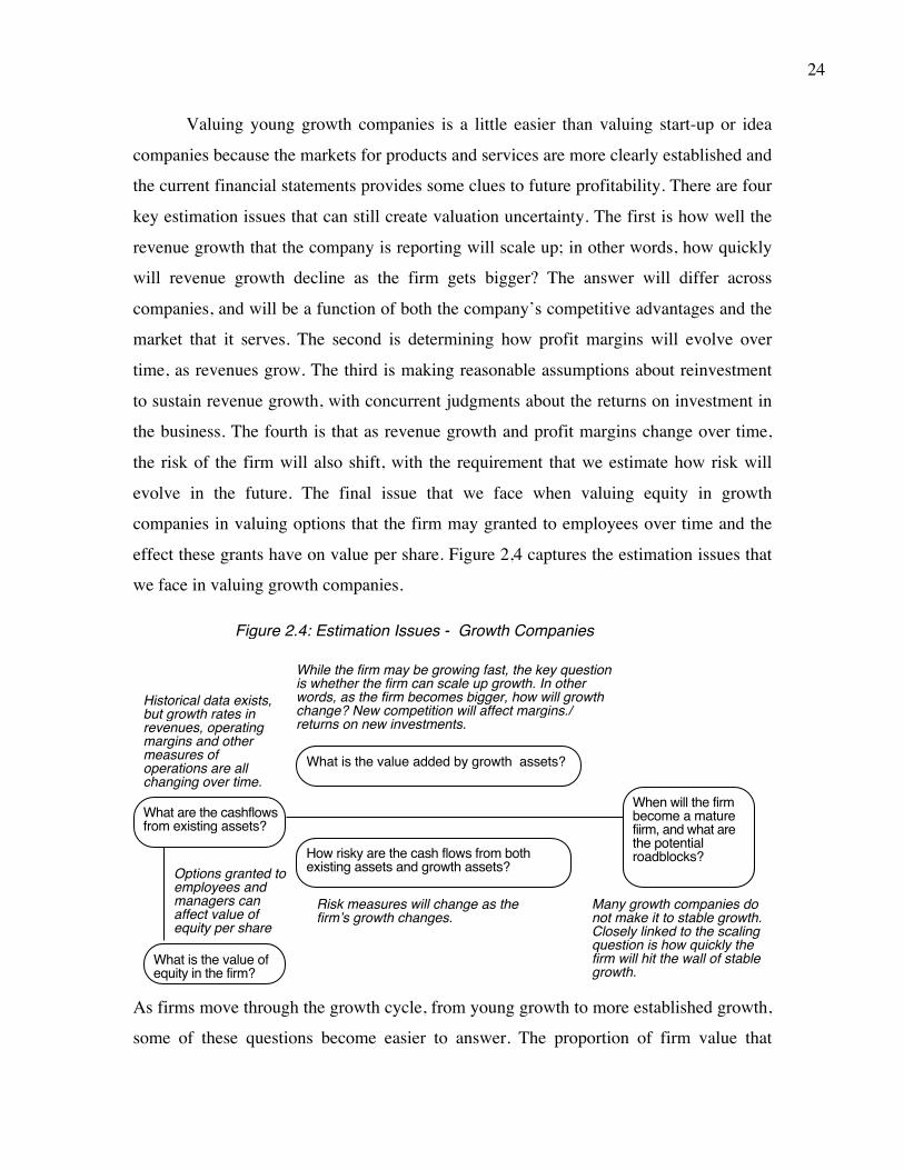
effect these grants have on value per share. Figure 2,4 captures the estimation issues that
we face in valuing growth companies.
As firms move through the growth cycle, from young growth to more established growth,
some of these questions become easier to answer. The proportion of firm value that
What are the cashflows from existing assets?
What is the value added by growth assets?
How risky are the cash flows from both existing assets and growth assets?
When will the firm become a mature fiirm, and what are the potential roadblocks?
Historical data exists, but growth rates in revenues, operating margins and other measures of operations are all changing over time.
Risk measures will change as the firmʼs growth changes.
While the firm may be growing fast, the key question is whether the firm can scale up growth. In other words, as the firm becomes bigger, how will growth change? New competition will affect margins./ returns on new investments.
Many growth companies do not make it to stable growth. Closely linked to the scaling question is how quickly the firm will hit the wall of stable growth.
Figure 2.4: Estimation Issues - Growth Companies
What is the value of equity in the firm?
Options granted to employees and managers can affect value of equity per share

25
comes from growth assets declines as existing assets become more profitable and also
account for a larger chunk of overall value.
Maturity – A mixed blessing: Mature firms
Even the best of growth companies reach a point where size works against them.
Their growth rates in revenues and earnings converge on the growth rate of the economy.
In this phase, the bulk of a firm’s value comes from existing investments, and financial
statements become more informative. Revenue growth is steady and profit margins have
settled into a pattern, making it easier to forecast earnings and cashflows.
While estimation does become simpler with these companies, there are potential
problems that analysts have to consider. The first is that the results from operations
(including revenues and earnings) reflect how well the firm is utilizing its existing assets.
Changes in operating efficiency can have large impacts on earnings and cash flows, even
in the near term. The second is that mature firms sometimes turn to acquisitions to
recreate growth potential, and predicting the magnitude and consequences of acquisitions
is much more difficult to do than estimating growth from organic or internal investments.
The third is that mature firms are more likely to look to financial restructuring to increase
their value; the mix of debt and equity used to fund the business may change overnight
and assets (such as accounts receivable) may be securitized. The final issue is that
mature companies sometimes have equity claims with differences in voting right and
control claims, and hence different values. Figure 2.5 frames the estimation challenges at
mature companies.

26
Not surprisingly, mature firms are usually targeted in hostile acquisitions and leveraged
buyouts, where the buyer believes that changing the way the firm is run can result in
significant increases in value.
Winding down: Dealing with decline Most firms reach a point in the life cycle, where their existing markets are
shrinking and becoming less profitable, and the forecast for the future is more of the
same. Under these circumstances, these firms react by selling assets and returning cash to
investors. Put another way, these firms derive their value entirely from existing assets and
that value is expected to shrink over time.
Valuing declining companies requires making judgments about the assets that will
be divested over time and the profitability of the assets that will be left in the firm.
Judgments about how much cash will be received in these divestitures and how that cash
will be utilized (pay dividends, buy back shares, retire debt) can influence the value
attached to the firm. There is another concern that overhangs this valuation. Some firms
in decline that have significant debt obligations can become distressed, a problem not
specific to declining firms but more common with them. Finally, the equity values in
What are the cashflows from existing assets?
What is the value added by growth assets?
How risky are the cash flows from both existing assets and growth assets?
When will the firm become a mature fiirm, and what are the potential roadblocks?
Lots of historical data on earnings and cashflows. Key questions remain if these numbers are volatile over time or if the existing assets are not being efficiently utilized.
Operating risk should be stable, but the firm can change its financial leverage This can affect both the cost of equtiy and capital.
Growth is usually not very high, but firms may still be generating healthy returns on investments, relative to cost of funding. Questions include how long they can generate these excess returns and with what growth rate in operations. Restructuring can change both inputs dramatically and some firms maintain high growth through acquisitions.
Maintaining excess returns or high growth for any length of time is difficult to do for a mature firm.
Figure 2.5: Estimation Issues - Mature Companies
What is the value of equity in the firm?
Equity claims can vary in voting rights and dividends.

27
declining firms can be affected significantly by the presence of underfunded pension
obligations and the overhand of litigation costs than other firms. In figure 2.6, we look at
these questions:
Valuing firms in decline poses a special challenge for analysts who are used to
conventional valuation models that adopt a growth-oriented view of the future. In other
words, assuming that current earnings will grow at healthy rates for the future or forever
will result in estimates of value for these firms that are way too high.
Valuation across the business spectrum In the last section, we considered the different issues we fact in estimating
cashflows, growth rates, risk and maturity across the business life cycle. In this section,
we consider how firms in some businesses are more difficult to value than others. We
consider five groups of companies – financial service firms such as banks, investment
banks and insurance companies, cyclical and commodity businesses, businesses with
intangible assets (human capital, patents, technology), emerging market companies that
face significant political risk and multi-business, global companies. With each group, we
examine what it is about the firms within the group that generate valuation problems.
What are the cashflows from existing assets?
What is the value added by growth assets?
How risky are the cash flows from both existing assets and growth assets?
When will the firm become a mature fiirm, and what are the potential roadblocks?
Historial data often reflects flat or declining revenues and falling margins. Investments often earn less than the cost of capital.
Depending upon the risk of the assets being divested and the use of the proceeds from the divestuture (to pay dividends or retire debt), the risk in both the firm and its equity can change.
Growth can be negative, as firm sheds assets and shrinks. As less profitable assets are shed, the firmʼs remaining assets may improve in quality.
There is a real chance, especially with high financial leverage, that the firm will not make it. If it is expected to survive as a going concern, it will be as a much smaller entity.
Figure 2.6: Estimation Issues - Declining Companies
What is the value of equity in the firm?
Underfunded pension obligations and litigation claims can lower value of equity. Liquidation preferences can affrect value of equity

28
Financial Service firms
While financial service firms have historically been viewed as stable investments
that are relatively simple to value, financial crises bring out the dangers in this
assumption. In 2008, for instance, the equity values at most banks swing wildly, and the
equity at many others including Lehman, Bear Stearns and Fortis lost all value. It was a
wake-up call to analysts who had used fairly simplistic models to value these banks and
had missed the brewing problems.
So what are the potential problems with valuing financial service firms? We can
frame them in terms of the four basic inputs into the valuation process. The existing
assets of banks are primarily financial assets, with a good portion being traded in
markets. While accounting rules require that these assets be marked to market, they are
not always consistently applied across different classes of assets. Since the risk in these
assets can vary widely across firms, and information about this risk is not always
forthcoming, accounting errors feed into valuation errors. The risk is magnified by the
high financial leverage at banks and investment banks, and it is not uncommon to see
banks have debt to equity ratios of 30 to 1 or higher, allowing them to leverage up the
profitability of their operations. Financial service firms are, for the most part, regulated,
and regulatory rules can affect growth potential. The regulatory restrictions on book
equity capital as a ratio of loans, at a bank, influences how quickly the bank can expand
over time and how profitable that expansion will be. Changes in regulatory rules will
therefore have big effects on growth and value, with more lenient (stricter) rules resulting
in more (less) value from growth assets. Finally, since the damage created by a troubled
bank or investment bank can be extensive, it is also likely that problems at these entities
will evoke much swifter reactions from authorities than at other firms. A troubled bank
will be quickly taken over to protect depositors, lenders and customers, but the equity in
the banks will be wiped out in the process. As a final point, getting to the value of equity
per share for a financial service firm can be complicated by the presence of preferred
stock, which shares characteristics with both debt and equity. Figure 2.7 summarizes the
valuation issues at financial service firms:

29
Analysts who value banks go through cycles. In good times, they tend to under estimate
the risk of financial crises and extrapolate from current profitability to arrive at higher
values for financial service firms. In crises, they lose perspective and mark down the
values of healthy banks and unhealthy banks, without much discrimination.
Cyclical and Commodity Companies If we define a mature company as one that delivers predictable earnings and
revenues, period after period, cyclical and commodity companies will never be mature,
since even the largest, most established of them have volatile earnings. The earnings
volatility has little to do with the company and is more reflective of variability in the
underlying economy (for cyclical firms) or the base commodity (for a commodity
company).
The biggest issue with valuing cyclical and commodity companies lies in the base
year numbers that are used in valuation. If we do what we do with most other companies
and use the current year as the base year, we risk building into our valuations the vagaries
of the economy or commodity prices in that year. As an illustration, valuing oil
companies, using earnings from 2007 as a base year, will inevitably result in too high a
value; the spike in oil prices that year contributed to the profitability of almost all oil
What are the cashflows from existing assets?
What is the value added by growth assets?
How risky are the cash flows from both existing assets and growth assets?
When will the firm become a mature fiirm, and what are the potential roadblocks?
Exisitng assets are usually financial assets or loans, often marked to market. Earnings do not provide much information on underlying risk.
Most financial service firms have high financial leverage, magnifying their exposure to operating risk. If operating risk changes significantly, the effects will be magnified on equity.
Growth can be strongly influenced by regulatory limits and constraints. Both the amount of new investments and the returns on these investments can change with regulatory changes.
In additioin to all the normal constraints, financial service firms also have to worry about maintaining capital ratios that are acceptable ot regulators. If they do not, they can be taken over and shut down.
Figure 2.7: Estimation Issues - Financial Service Firms
What is the value of equity in the firm?
Preferred stock is a significant source of capital.
30
companies, small and large, efficient and inefficient. Similarly valuing housing
companies, using earnings and other numbers from 2008, when the economy was
drastically slowing down, will result in values that are too low. The uncertainty we feel
about base year earnings also percolates into other parts of the valuation. Estimates of
growth at cyclical and commodity companies depend more on our views on overall
economic growth and the future of commodity prices than they do on the investments
made at individual companies. Similarly, risk that lies dormant when the economy is
doing well and commodity prices are rising can manifest itself suddenly when the cycle
turns. Finally, for highly levered cyclical and commodity companies, especially when the
debt was accumulated during earnings upswings, a reversal of fortune can very quickly
put the firm at risk. In addition, for companies like oil companies, the fact that natural
resources are finite – there is only so much oil under the ground – can put a crimp on
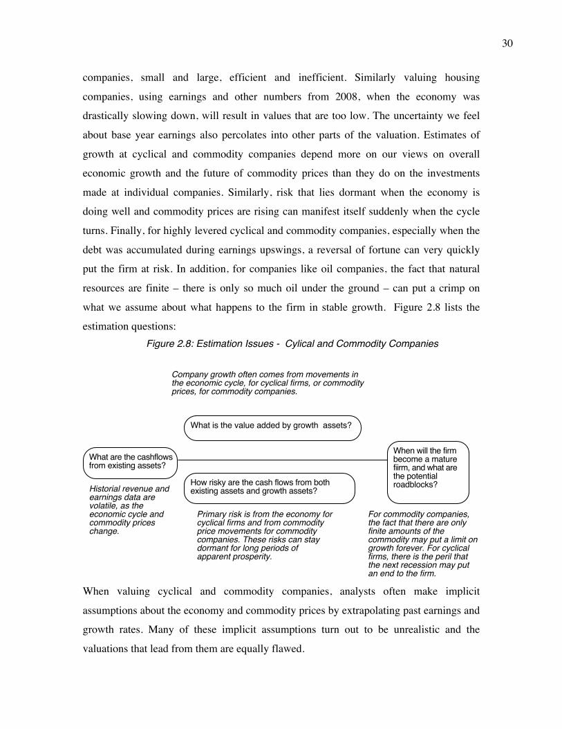
what we assume about what happens to the firm in stable growth. Figure 2.8 lists the
estimation questions:
When valuing cyclical and commodity companies, analysts often make implicit
assumptions about the economy and commodity prices by extrapolating past earnings and
growth rates. Many of these implicit assumptions turn out to be unrealistic and the
valuations that lead from them are equally flawed.
What are the cashflows from existing assets?
What is the value added by growth assets?
How risky are the cash flows from both existing assets and growth assets?
When will the firm become a mature fiirm, and what are the potential roadblocks?Historial revenue and
earnings data are volatile, as the economic cycle and commodity prices change.
Primary risk is from the economy for cyclical firms and from commodity price movements for commodity companies. These risks can stay dormant for long periods of apparent prosperity.
Company growth often comes from movements in the economic cycle, for cyclical firms, or commodity prices, for commodity companies.
For commodity companies, the fact that there are only finite amounts of the commodity may put a limit on growth forever. For cyclical firms, there is the peril that the next recession may put an end to the firm.
Figure 2.8: Estimation Issues - Cylical and Commodity Companies
31
Businesses with Intangible Assets
In the last two decades, we have seen mature economies, such as the US and
Western Europe, shift away from manufacturing to service and technology businesses. In
the process, we have come to recognize how little of the value at many of our largest
companies today comes not from physical assets (like land, machinery and factories) and
how much of the value comes from intangible assets. Intangible assets range the
spectrum, from brand name at Coca Cola to technological know-how at Google and
human capital at firms like McKinsey. As accountants grapple with how best to deal with
these intangible assets, we fact similar challenges when valuing them.
Let us state at the outset that there should be no reason why the tools that we have
developed over time for physical assets cannot be applied to intangible assets. The value
of a brand name or patent should be the present value of the cash flows from that asset,
discounted back at an appropriate risk adjusted rate. The problem that we face is that the
accounting standards for firms with intangible assets are not entirely consistent with the
standards for firms with physical assets. An automobile company that invests in a new
plant/factory is allowed to treat that expenditure as a capital expenditure, record the item
as an asset and depreciate it over its life. A technology firm that invests in research and
development, with the hope of generating new patents, is required to expense the entire
expenditure, record no assets and cannot amortize or depreciate the item. The same can
be said of a consumer product company that expends millions on advertising with the
intent of building up a brand name. The consequences for estimating the basic inputs for
valuation are profound. For existing assets, the accounting treatment of intangible assets
makes both current earnings and book value unreliable, since the former is net of R&D
and the latter does not include investments in the firm’s biggest assets. Since
reinvestment and accounting return numbers are flawed for the same reasons, assessing
expected growth becomes more difficult. Since lenders tend to be wary about lending to
firms with intangible assets, they tend to be funded predominantly with equity, and the
risk of equity can change quickly over a firm’s life cycle. Finally, estimating when a firm
with intangible assets gets to steady state can be complex. On the one hand, easy entry
into and exit from the business and rapid changes in technology can cause growth rates to
drop quickly at some firms. On the other hand, the long life of some competitive

32
advantages like brand name and the ease with which firms can scale up (they do not need
heavy infrastructure or physical investments) can allow other firms to maintain high
growth, with excess returns, for decades. The problems that we face in valuing companies
with intangible assets are shown in figure 2.9:
Analysts when faced with valuing firms with intangible assets tend to use the accounting
earnings and book values at these firms, without correcting for the miscategorization of
capital expenditures. Any analyst who compares the PE ratio for Microsoft to the PE ratio
for GE is guilty of this error. In addition, there is also the temptation, when doing
valuations, to add arbitrary premiums to estimated value to reflect the value of
intangibles. Thus, adding a 30% premium to the value estimate of Coca Cola is not a
sensible way of capturing the value of a brand name.
Emerging Market Companies
In the last decade, the economies that have grown the fastest have been in Asia
and Latin America. With that growth, we have also seen an explosion of listings in
What are the cashflows from existing assets?
What is the value added by growth assets?
How risky are the cash flows from both existing assets and growth assets?
When will the firm become a mature fiirm, and what are the potential roadblocks?The capital
expenditures associated with acquiring intangible assets (technology, himan capital) are mis-categorized as operating expenses, leading to inccorect accounting earnings and measures of capital invested.
It ican be more difficult to borrow against intangible assets than it is against tangible assets. The risk in operations can change depending upon how stable the intangible asset is.
If capital expenditures are miscategorized as operating expenses, it becomes very difficult to assess how much a firm is reinvesting for future growth and how well its investments are doing.
Intangible assets such as brand name and customer loyalty can last for very long periods or dissipate overnight.
Figure 2.9: Estimation Issues - Intangible Assets

33
financial markets in these emerging economies and increased interest in valuing
companies in these markets.
In valuing emerging market companies, the overriding concern that analysts have
is that the risk of the countries that these companies operate in often overwhelms the risk
in the companies themselves. Investing in a stable company in Argentina will still expose
you to considerable risk, as country risk swings back and forth. While the inputs to
valuing emerging market companies are familiar – cashflows from existing and growth
assets, risk and getting to stable growth – country risk creates estimation issues with each
input. Variations in accounting standards and corporate governance rules across emerging
markets often result in lack of transparency when it comes to current earnings and
investments, making it difficult to assess the value of existing assets. Expectations of
future growth rest almost as much on how the emerging market that the company is
located will evolve, as they do on the company’s own prospects. Put another way, it is
difficult for even the best-run emerging market company to grow, if the market it
operates in is in crisis. In a similar vein, the overlay of country risk on company risk
indicates that we have to confront and measure both, if we want to value emerging
market companies. Finally, in addition to economic crises that visit emerging markets at
regular intervals, putting all companies at risk, there is also the added risk that companies
can be nationalized or appropriated by the government. The challenges associated with
valuing emerging market companies are captured in figure 2.10:

34
Analysts who value emerging market companies develop their own coping mechanisms
for dealing with the overhang of country, with some mechanisms being healthier than
others. In its most unhealthy form, analysts avoid even dealing with the risk, switching to
more stable currencies for their valuations and adopting very simplistic measures of
country risk (such as adding a fixed premium to every company in a market). In other
cases, their pre-occupation with country risk leads them to double count and triple count
the risk and not pay sufficient attention to the company being valued.
Multi-business and Global companies As investors globalize their portfolios, companies are also becoming increasingly
globalized, with many of the largest ones operating in multiple businesses. Give that
these businesses have very different risk and operating characteristics, valuing the multi-
business, global company can be a challenge even to the best-prepared analyst.
The conventional approach to valuing a company has generally been to work with
the consolidated earnings and cashflows of the business, and discount those cash flows
using an aggregated risk measure for the company that reflects its mix of businesses.
While this approach works well for firms in one or few lines of business, it becomes
increasingly difficult as companies spread their operations across multiple businesses in
multiple markets. Consider a firm like General Electric, a conglomerate that operates in
What are the cashflows from existing assets?
What is the value added by growth assets?
How risky are the cash flows from both existing assets and growth assets?
When will the firm become a mature fiirm, and what are the potential roadblocks?
Big shifts in economic environment (inflation, itnerest rates) can affect operating earnings history. Poor corporate governance and weak accounting standards can lead to lack of transparency on earnings.
Even if the companyʼs risk is stable, there can be significant changes in country risk over time.
Growth rates for a company will be affected heavily be growth rate and political developments in the country in which it operates.
Economic crises can put many companies at risk. Government actions (nationalization) can affect long term value.
Figure 2.10: Estimation Issues - Emerging Market Companies
What is the value of equity in the firm?
Cross holdings can affect value of equity

35
dozens of businesses and in almost every country on the globe. The financial statements
of the company reflect its aggregated operations, across its different businesses and
geographic locations. Attaching a value to existing assets becomes difficult to do, since
these assets vary widely in terms of risk and return generating capacity. While GE may
break down earnings for its different business lines, those numbers are contaminated by
the accounting allocation of centralized costs and intra-business transactions. The
expected growth rates can be very different for different parts of the business, not only in
terms of magnitude but also in quality. Furthermore, as the firm grows at different rates
in different businesses, its overall risk will change to reflect the new business weights,
adding another problem to valuation. Finally, different pieces of the company may
approach stable growth at different points in time, making it difficult to stop and assess
the terminal value. Figure 2.11 summarizes the estimation questions that we have to
answer for complex companies.
Analysts who value multi-business and global companies often draw on the averaging
argument to justify not knowing as much as they should about individual businesses.
Higher growth (risk) in some businesses will be offset by lower growth (risk) in other
businesses, they argue, thus justifying their overall estimates of growth and risk. They
What are the cashflows from existing assets?
What is the value added by growth assets?
How risky are the cash flows from both existing assets and growth assets?
When will the firm become a mature fiirm, and what are the potential roadblocks?The firm reports
aggregate earnings from its investments in many businesses and many countries as well as in many currencies. Breakdown of earnings and operating variables in either incomplete or misleading.
Since risk can vary widely depending upon the cash flow stream, estimating one cost of equity and capital for a multi-business, global company that can be maintained over time is an exercise in futility.
Growth rates can vary widely across busineses and across countries. Trying to estimate “one” growth rate fro a firm can be difficult to do.
Different parts of the company will reach stable growth at different points in time.
Figure 2.11: Estimation Issues - Multi -business and Global Businesses

36
underestimate the dangers of the unknown. All too often, with companies like these, what
you do not know is more likely to contain bad news than good news.
Conclusion Some companies are easier to value than others. When we have to leave the
comfort zone of companies with solid earnings and predictable futures, we invariably
stray into the dark side of valuation, where we invent new principles, violate established
ones and come up with unsustainable values for businesses.
In this chapter, we laid out the four inputs that we have to estimate to value any
company – the expected cash from investments that the business has already made
(existing assets), the value that will be added by new investments (growth assets), the risk
in these cash flows and the point in time where we expect the firm to become a mature
firm. The estimation challenges we face will vary widely across companies and we
consider how estimation issues vary across the life cycle of a firm. For young and start-up
firms, the absence of historical data and the dependence on growth assets makes
estimating future cash flows and risk particularly difficult to do. With growth firms, the
question shifts to whether growth rates can be maintained and, if so, for how long, as
firms scale up. With mature firms, the big issue in valuation shifts to whether existing
assets are being efficiently utilized and whether the financial mix used by the firm makes
sense; restructuring the firm to make it better run may dramatically alter value. For
declining firms, estimating revenues and margins as assets get divested, while also
considering the possibility of default can be tricky. The estimation challenges we face
can also be different for different subsets of companies – cyclical and commodity
companies have volatile operating results, companies with intangible assets have earnings
that are skewed by how accountants treat investments in these assets, and the risk in
emerging market and global companies can be difficult to assess. Finally, valuing any
company can become more difficult in economies where the fundamentals – riskfree
rates, risk premiums and economic growth – are volatile.

37
CHAPTER 3
INTRINSIC VALUATION: THE COST OF CAPITAL (WACC)
APPROACH In discounted cashflows valuation, the value of an asset is the present value of the
expected cashflows on the asset, discounted back at a rate that reflects the riskiness of
these cashflows. In chapter 1, we noted the distinction between valuing a business and
valuing equity in the business. In this section, we will focus on how best to value a
business, using the cost of capital approach.
Determinants of Value While you can choose to value just the equity or the entire business, there are
four basic inputs that you need for a value estimate, though how you define the inputs
will be different depending upon whether you do firm or equity valuation. Figure 3.1
summarizes the determinants of value.
The first input is the cashflow from existing assets, defined either as pre-debt (and to the
firm) or as post-debt (and to equity) earnings, net of reinvestment to generate future
growth. With equity cashflows, we can use an even stricter definition of cash flow and
consider only dividends paid. The second input is growth, with growth in operating
income being the key input when valuing the entire business and growth in equity income
(net income or earnings per share) becoming the focus when valuing equity. The third
Current CashflowsThese are the cash flows from existing investment,s, net of any reinvestment needed to sustain future growth. They can be computed before debt cashflows (to the firm) or after debt cashflows (to equity investors).
Expected Growth during high growth period
Growth from new investmentsGrowth created by making new investments; function of amount and quality of investments
Efficiency GrowthGrowth generated by using existing assets better
Length of the high growth periodSince value creating growth requires excess returns, this is a function of- Magnitude of competitive advantages- Sustainability of competitive advantages
Stable growth firm, with no or very limited excess returns
Cost of financing (debt or capital) to apply to discounting cashflowsDetermined by- Operating risk of the company- Default risk of the company- Mix of debt and equity used in financing
Figure 3.1: Determinants of Value
Terminal Value of firm (equity)

38
input is the discount rate, defined as the cost of the overall capital of the firm, when
valuing the business, and as cost of equity, when valuing equity. The final input, allowing
for closure, is the terminal value, defined as the estimated value of firm (equity) at the
end of the forecast period in firm (equity) valuation.
For the rest of this section, we will focus on estimating the inputs into firm
valuation models, starting with the cashflows, moving on to risk (and discount rates) and
then closing with a discussion of how best to estimate the growth rate for the high growth
period and the value at the end of that period.
Cash Flows When valuing a business, as opposed to just the equity stake in the business, we
begin by separating the operating assets of the business from its cash and marketable
securities and estimating the cash flows from those operating assets. This operating cash
flow, which is generally called the free cash flow to the firm (FCFF) should be both after
taxes and after all reinvestment needs have been met. Since a firm raises capital from
debt and equity investors, the cash flow to the firm should be before interest and principal
payments on debt.
To estimate the free cash flow to the firm, we start with after-tax operating
earnings and to estimate the cash flows to the firm prior to debt payments but after
reinvestment needs have been met:
Step 1: To estimate the operating earnings after taxes, we start with the reported earnings
before interest and taxes (EBIT) and estimate the taxes we would have paid if this income
had been the taxable income.
After-tax operating income = EBIT (1- tax rate)
There are two points to note about this measure. The first is that the tax rate used to
compute after-tax income can be much lower than the statutory tax rate in the near term,
but that gap will narrow over time, as the company matures. The second is that the actual
taxes paid can and often is much lower than the hypothetical tax that we are estimating in
the computation. This will especially be true for firms with substantial interest expenses,
since these expenses can reduce taxable income and taxes. We are intentionally ignoring

39
the tax benefits accruing from interest expenses, when computing cash flows, because we
will consider these same tax benefits, when computing the discount rate (cost of capital).
Step 2: To estimate reinvestment, we will break it down into two parts:
a. Reinvestment in long-lived assets is measured as the difference between capital
expenditures (the amount invested in long lived assets during the period) and
depreciation (the accounting expense generated by capital expenditures in prior
periods). We net the latter because it is not a cash expense and hence can be added
back to net income.
b. Reinvestment in short-lived assets is measured by the change in non-cash working
capital. In effect, increases in inventory and accounts receivable represent cash tied
up in assets that do not generate returns – wasting assets. The reason we done
consider cash in the computation is because we assume that companies with large
cash balances generally invest them in low-risk, marketable securities like
commercial paper and treasury bills; these investments earn a low but a fair rate of
return and are therefore not wasting assets.3 To the extent that they are offset by the
use of supplier credit and accounts payable, the effect on cash flows can be muted.
The overall change in non-cash working capital (Δ NWC) therefore is investment in
short-term assets.
In summary, the free cash flow to the firm can be written as:
FCFF = EBIT (1-t)– (Capital Expenditures –Depreciation) - Δ NWC
Reinvestment reduces the free cash flow, but it provides a payoff in terms of future
growth. We will come back and consider whether the net effect is positive or negative
after we consider how best to estimate growth.
Another way of presenting the same equation is to cumulate the net capital expenditures
and working capital change into one number, and state it as a percentage of the after-tax
operating income. This ratio of reinvestment to after-tax operating income is called the
reinvestment rate, and the free cash flow to the firm can be written as: 3 Note that we do not make the distinction between operating and non-operating cash that some analysts do
(they proceed to include operating cash in working capital). Our distinction is between wasting cash (which
would include currency or cash earning below-market rate returns) and non-wasting cash. We are assuming
that the former will be a small or negligible number at a publicly traded company.
40
Reinvestment Rate =
€
(Capital Expenditures - Depreciation + Δ Working Capital)After - tax Operating Income
Free Cash Flow to the Firm = EBIT (1-t) (1 – Reinvestment Rate)
Note that the reinvestment rate can exceed 100%4, if the firm has substantial reinvestment
needs. The reinvestment rate can also be less than zero, for firms that are divesting assets
and shrinking capital.
A few final thoughts about free cash flow to the firm are worth noting before we
move on to discount rates. First, the free cash flow to the firm can be negative, just as the
FCFE can, but debt cash flows can no longer be the culprit; even highly levered firms
that are paying down debt will report positive FCFF while also registering negative
FCFE. If the FCFF is negative, the firm will be raising fresh capital, with the mix of debt
and equity being determined by the mix used to compute the cost of capital. Second, the
cash flow to the firm is the basis for all cash distributions made by the firm to its
investors; dividends, stock buybacks, interest payments and debt repayments all have to
be made out of these cash flows.
Risk Cash flows that are riskier should be assessed a lower value than more stable
cashflows, but how do we measure risk and reflect it in value? In conventional
discounted cash flow valuation models, the discount rate becomes the vehicle for
conveying our concerns about risk. We use higher discount rates on riskier cash flows
and lower discount rates on safer cash flows. In this section, we will begin be contrasting
how the risk in equity can vary from the risk in a business, and then consider the
mechanics of estimating the cost of equity and capital.
Business Risk versus Equity Risk
Before we delve into the details of risk measurement and discount rates, we
should draw a contrast between two different ways of thinking about risk that relate back
to the financial balance sheet that we presented in chapter 1. In the first, we think about
4 In practical terms, this firm will have to raise external financing, either from debt or equity or both, to
cover the excess reinvestment.
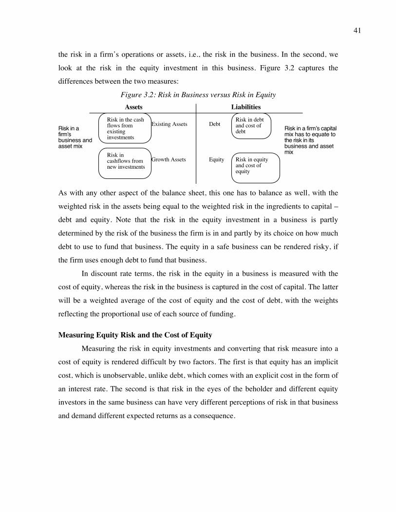
41
the risk in a firm’s operations or assets, i.e., the risk in the business. In the second, we
look at the risk in the equity investment in this business. Figure 3.2 captures the
differences between the two measures:
Figure 3.2: Risk in Business versus Risk in Equity
As with any other aspect of the balance sheet, this one has to balance as well, with the
weighted risk in the assets being equal to the weighted risk in the ingredients to capital –
debt and equity. Note that the risk in the equity investment in a business is partly
determined by the risk of the business the firm is in and partly by its choice on how much
debt to use to fund that business. The equity in a safe business can be rendered risky, if
the firm uses enough debt to fund that business.
In discount rate terms, the risk in the equity in a business is measured with the
cost of equity, whereas the risk in the business is captured in the cost of capital. The latter
will be a weighted average of the cost of equity and the cost of debt, with the weights
reflecting the proportional use of each source of funding.
Measuring Equity Risk and the Cost of Equity
Measuring the risk in equity investments and converting that risk measure into a
cost of equity is rendered difficult by two factors. The first is that equity has an implicit
cost, which is unobservable, unlike debt, which comes with an explicit cost in the form of
an interest rate. The second is that risk in the eyes of the beholder and different equity
investors in the same business can have very different perceptions of risk in that business
and demand different expected returns as a consequence.
Assets Liabilities
Existing Assets Debt
Equity
Risk in debt and cost of debt
Risk in equity and cost of equity
Growth Assets
Risk in the cash flows from existing investments
Risk in cashflows from new investments
Risk in a firmʼs business and asset mix
Risk in a firmʼs capital mix has to equate to the risk in its business and asset mix

42
The Diversified Marginal Investor
If there were only one equity investor in a company, estimating equity risk and
the cost of equity would be a far simpler exercise. We would measure the risk of
investing in equity in that company to the investor and assess a reasonable rate of return,
given that risk. In a publicly traded company, we run into the practical problem that the
equity investors number in the hundreds, if not the thousands, and that they not only vary
in size, from small to large investors, but also in risk aversion. So, whose perspective
should we take when measuring risk and cost of equity? In corporate finance and
valuation, we develop the notion of the marginal investor, i.e., the investor most likely to
influence the market price of publicly traded equity. The marginal investor in a publicly
traded stock has to own enough stock in the company to make a difference and be willing
to trade on that stock. The common theme shared by risk and return models in finance is
that the marginal investor is diversified, and we measure the risk in an investment as the
risk added to a diversified portfolio. Put another way, it is only that portion of the risk in
an investment that is attributable to the broader market or economy, and hence not
diversifiable, that should be built into expected returns.
Models for Expected Return (Cost of Equity)
It is on the issue of how best to measure this non-diversifiable risk that the
different risk and return models in finance part ways. Let use consider the alternatives:
• In the capital asset pricing model (CAPM), this risk is captured in the beta that we
assign an asset/business, with that number carrying the burden of measuring exposure
to all of the components of market risk. The expected return on an investment can
then be specified as a function of three variables – the riskfree rate, the beta of the
investment and the equity risk premium (the premium demanded for investing in the
average risk investment):
Expected Return = Riskfree Rate + BetaInvestment (Equity Risk Premium)
The riskfree rate and equity risk premium are the same for all investments in a market
but the beta will capture the market risk exposure of the investment; a beta of one
represents an average risk investment, and betas above (below) one indicate
investments that are riskier (safer) than the average risk investment in the market.

43
• In the arbitrage pricing and multi-factor models, we allow for multiple sources of
non-diversifiable (or market) risk and estimate betas against each one. The expected
return on an investment can be written as a function of the multiple betas (relative to
each market risk factor) and the risk premium for that factor. If there are k factors in
the model with βji and Risk Premiumj representing the beta and risk premium of
factor j, the expected return on the investment can be written as:
Expected Return =
€
Riskfree Rate + β jj=1
j=k
∑ (Risk Premiumj)
Note that the capital asset pricing model can be written as a special case of these
multi-factor models, with a single factor (the market) replacing the multiple factors.
• The final class of models can be categorized as proxy models. In these models, we
essentially give up on measuring risk directly and instead look at historical data for
clues on what types of investments (stocks) have earned high returns in the past, and
then use the common characteristic(s) that they share as a measure of risk. For
instance, researchers have found that market capitalization and price to book ratios
are correlated with returns; stocks with small market capitalization and low price to
book ratios have historically earned higher returns than large market stocks with
higher price to book ratios. Using the historical data, we can then estimate the
expected return for a company, based on its market capitalization and price to book
ratio.
Expected Return = a + b(Market Capitalization) + c (Price to Book Ratio)
Since we are no longer working within the confines of an economic model, it is not
surprising that researchers keep finding new variables (trading volume, price
momentum) that improve the predictive power of these models. The open question,
though, is whether these variables are truly proxies for risk or indicators of market
inefficiency. In effect, we may be explaining away the misvaluatiion of classes of
stock by the market by using proxy models for risk.
Estimation Issues
With the CAPM and multi-factor models, the inputs that we need for the expected
return are straightforward. We need to come up with a risk free rate and an equity risk
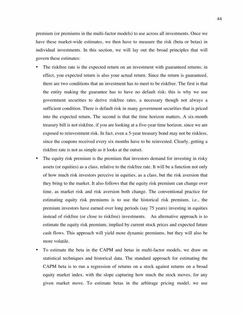
44
premium (or premiums in the multi-factor models) to use across all investments. Once we
have these market-wide estimates, we then have to measure the risk (beta or betas) in
individual investments. In this section, we will lay out the broad principles that will
govern these estimates:
• The riskfree rate is the expected return on an investment with guaranteed returns; in
effect, you expected return is also your actual return. Since the return is guaranteed,
there are two conditions that an investment has to meet to be riskfree. The first is that
the entity making the guarantee has to have no default risk; this is why we use
government securities to derive riskfree rates, a necessary though not always a
sufficient condition. There is default risk in many government securities that is priced
into the expected return. The second is that the time horizon matters. A six-month
treasury bill is not riskfree, if you are looking at a five-year time horizon, since we are
exposed to reinvestment risk. In fact, even a 5-year treasury bond may not be riskless,
since the coupons received every six months have to be reinvested. Clearly, getting a
riskfree rate is not as simple as it looks at the outset.
• The equity risk premium is the premium that investors demand for investing in risky
assets (or equities) as a class, relative to the riskfree rate. It will be a function not only
of how much risk investors perceive in equities, as a class, but the risk aversion that
they bring to the market. It also follows that the equity risk premium can change over
time, as market risk and risk aversion both change. The conventional practice for
estimating equity risk premiums is to use the historical risk premium, i.e., the
premium investors have earned over long periods (say 75 years) investing in equities
instead of riskfree (or close to riskfree) investments. An alternative approach is to
estimate the equity risk premium, implied by current stock prices and expected future
cash flows. This approach will yield more dynamic premiums, but they will also be
more volatile.
• To estimate the beta in the CAPM and betas in multi-factor models, we draw on
statistical techniques and historical data. The standard approach for estimating the
CAPM beta is to run a regression of returns on a stock against returns on a broad
equity market index, with the slope capturing how much the stock moves, for any
given market move. To estimate betas in the arbitrage pricing model, we use

45
historical return data on stocks and factor analysis to extract both the number of
factors in the models, as well as factor betas for individual companies. As a
consequence, the beta estimates that we obtain will always be backward looking
(since they are derived from past data) and noisy (they are statistical estimates, with
standard errors). In addition, these approaches clearly will not work for investments
that do not have a trading history (young companies, divisions of publicly traded
companies). One solution is to replace the regression beta with a bottom-up beta, i.e.,
a beta that is based upon industry averages for the businesses that the firm is in,
adjusted for differences in financial leverage.5 Since industry averages are more
precise than individual regression betas, and the weights on the businesses can reflect
the current mix of a firm, bottom up betas generally offer better estimates for the
future.
The Cost of Debt While equity investors receive residual cash flows and bear the bulk of the
operating risk in most firms, lenders to the firm also face the risk that they will not
receive their promised payments – interest expenses and principal repayments. It is to
cover this default risk that lenders add a “default spread” to the riskless rate when they
lend money to firms; the greater the perceived risk of default, the greater the default
spread and the cost of debt. The other dimension on which debt and equity can vary is in
their treatment for tax purposes, with cashflows to equity investors (dividends and stock
buybacks) coming from after-tax cash flows, whereas interest payments are tax
deductible. In effect, the tax law provides a benefit to debt and lowers the cost of
borrowing to businesses.
5 The simplest and most widely used equation relating betas to debt to equity ratios is based on the
assumption that debt provides a tax advantage and that the beta of debt is zero.
Beta for equity = Beta of business * (1+ (1- tax rate) (Debt/ Equity))
The beta for equity is a levered beta, whereas the beta of the business is titled an unlevered beta. Regression
betas are equity betas and are thus levered – the debt to equity ratio over the regression period is embedded
in the beta.
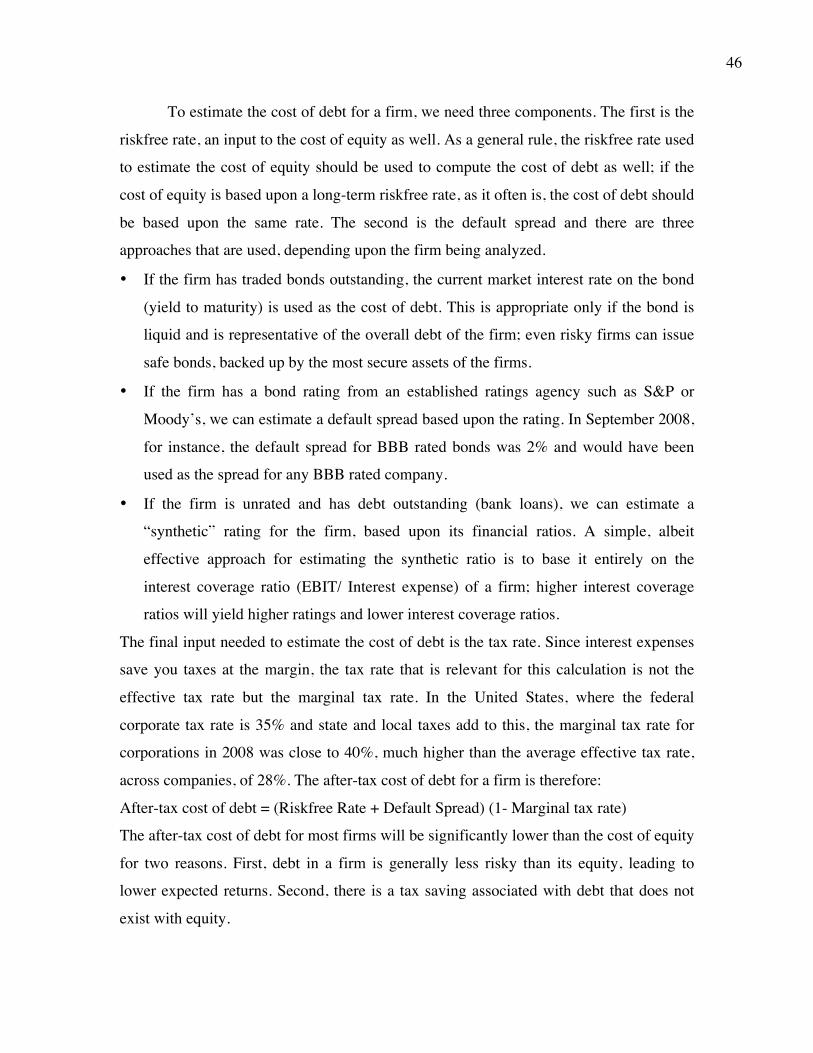
46
To estimate the cost of debt for a firm, we need three components. The first is the
riskfree rate, an input to the cost of equity as well. As a general rule, the riskfree rate used
to estimate the cost of equity should be used to compute the cost of debt as well; if the
cost of equity is based upon a long-term riskfree rate, as it often is, the cost of debt should
be based upon the same rate. The second is the default spread and there are three
approaches that are used, depending upon the firm being analyzed.
• If the firm has traded bonds outstanding, the current market interest rate on the bond
(yield to maturity) is used as the cost of debt. This is appropriate only if the bond is
liquid and is representative of the overall debt of the firm; even risky firms can issue
safe bonds, backed up by the most secure assets of the firms.
• If the firm has a bond rating from an established ratings agency such as S&P or
Moody’s, we can estimate a default spread based upon the rating. In September 2008,
for instance, the default spread for BBB rated bonds was 2% and would have been
used as the spread for any BBB rated company.
• If the firm is unrated and has debt outstanding (bank loans), we can estimate a
“synthetic” rating for the firm, based upon its financial ratios. A simple, albeit
effective approach for estimating the synthetic ratio is to base it entirely on the
interest coverage ratio (EBIT/ Interest expense) of a firm; higher interest coverage
ratios will yield higher ratings and lower interest coverage ratios.
The final input needed to estimate the cost of debt is the tax rate. Since interest expenses
save you taxes at the margin, the tax rate that is relevant for this calculation is not the
effective tax rate but the marginal tax rate. In the United States, where the federal
corporate tax rate is 35% and state and local taxes add to this, the marginal tax rate for
corporations in 2008 was close to 40%, much higher than the average effective tax rate,
across companies, of 28%. The after-tax cost of debt for a firm is therefore:
After-tax cost of debt = (Riskfree Rate + Default Spread) (1- Marginal tax rate)
The after-tax cost of debt for most firms will be significantly lower than the cost of equity
for two reasons. First, debt in a firm is generally less risky than its equity, leading to
lower expected returns. Second, there is a tax saving associated with debt that does not
exist with equity.

47
Debt Ratios and the Cost of Capital
Once we have estimated the costs of debt and equity, we still have to assign
weights for the two ingredients. To come up with this value, we could start with the mix
of debt and equity that the firm uses right now. In making this estimate, the values that
we should use are market values, rather than book values. For publicly traded firms,
estimating the market value of equity is usually a trivial exercise, where we multiply the
share price by the number of shares outstanding. Estimating the market value of debt is
usually a more difficult exercise, since most firms have some debt that is not traded.
Though many practitioners fall back on book value of debt as a proxy of market value,
estimating the market value of debt is still a better practice.
Once we have the current market value weights for debt and equity for use in the
cost of capital, we have a follow up judgment to make in terms of whether these weights
will change or remain stable. If we assume that they will change, we have to specify both
what the right or target mix for the firm will be and how soon the change will occur. In
an acquisition, for instance, we can assume that the acquirer can replace the existing mix
with the target mix instantaneously. As passive investors in publicly traded firms, we
have to be more cautious, since we do not control how a firm funds its operations. In this
case, we may adjust the debt ratio from the current mix to the target over time, with
concurrent changes in the costs of debt, equity and capital. In fact, the last point about
debt ratios and costs of capital changing over time is worth reemphasizing. As companies
change over time, we should expect the cost of capital to change as well.
Growth Rates There is no other ingredient in discounted cash flow valuation that evokes as
much angst as estimating future growth. Unlike cash flows and discount rates, where we
often have the security of historical data, growth rates require us to grapple with the
future. In this section, we will examine two of the standard approaches for estimating
growth (by looking at the past and using analyst estimates) and close with a discussion of
the fundamentals that determine growth.

48
Historical and Forecasted Growth Rates
When confronted with the task of estimating growth, it is not surprising that
analysts turn to the past. In effect, they use growth in revenues or earnings in the recent
past as a predictor of growth in the future. Before we put this practice under the
microscope, we should add that the historical growth rates for the same company can
yield different estimates n for the following reasons:
1. Earnings measure: The growth rates in earnings per share, net income, operating
income and revenues can be very different for the same firm over a specified time
period.
2. Period of analysis: For firms that have been in existence for long periods, the growth
rates can be very different if we look at ten years of history as opposed to five years.
3. Averaging approach: Even if we agree on an earnings measure and time period for the
analysis, the growth rates we derive can be different, depending upon how we
compute the values. We could, for instance, compute the growth rate in each period
and average the growth rates over time, yielding an arithmetic average. Alternatively,
we could use just the starting and ending values for the measure and compute a
geometric average. For firms with volatile earnings, the latter can generate a very
different (and lower) value for growth than the former.
A debate how best to estimate historical growth makes sense only if it is a good predictor
of future growth. Unfortunately, studies that have looked at the relationship have
generally concluded that (a) the relationship between past and future growth is a very
weak one, (b) scaling matters, with growth dropping off significantly as companies grow
and (c) firms and sectors grow through growth cycles, with high growth in one period
followed by low growth in the next.
If historical growth is not a useful predictor of future growth, there is another
source that we can use for future growth. We can draw on those who know the firm better
than we do – equity research analysts who have tracked the firm for years or the
managers in the firm – and use their estimates of growth. On the plus side, these forecasts
should be based upon better information than we have available to us. After all, managers
should have a clearer sense of how much they will reinvest in their own businesses and
what the potential returns on investments are when they do, and equity research analysts
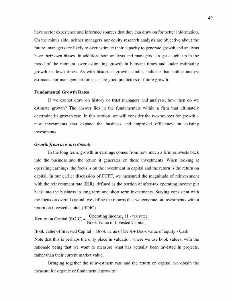
49
have sector experience and informed sources that they can draw on for better information.
On the minus side, neither managers nor equity research analysts are objective about the
future; managers are likely to over estimate their capacity to generate growth and analysts
have their own biases. In addition, both analysts and managers can get caught up in the
mood of the moment, over estimating growth in buoyant times and under estimating
growth in down times. As with historical growth, studies indicate that neither analyst
estimates nor management forecasts are good predictors of future growth.
Fundamental Growth Rates
If we cannot draw on history or trust managers and analysts, how then do we
estimate growth? The answer lies in the fundamentals within a firm that ultimately
determine its growth rate. In this section, we will consider the two sources for growth –
new investments that expand the business and improved efficiency on existing
investments.
Growth from new investments
In the long term, growth in earnings comes from how much a firm reinvests back
into the business and the return it generates on these investments. When looking at
operating earnings, the focus is on the investment in capital and the return is the return on
capital. In our earlier discussion of FCFF, we measured the magnitude of reinvestment
with the reinvestment rate (RIR), defined as the portion of after-tax operating income put
back into the business in long term and short term investments. Staying consistent with
the focus on overall capital, we define the returns that we generate on investments with a
return on invested capital (ROIC)
Return on Capital (ROIC) = Operating Incomet (1 - tax rate)Book Value of Invested Capitalt-1
Book value of Invested Capital = Book value of Debt + Book value of equity - Cash
Note that this is perhaps the only place in valuation where we use book values, with the
rationale being that we want to measure what has actually been invested in projects,
rather than their current market value.
Bringing together the reinvestment rate and the return on capital, we obtain the
measure for organic or fundamental growth:
50
Expected Growth in operating income = Reinvestment Rate * ROIC
There are two issues that arise in this estimate. The first is that uaccounting
measures (earnings and book value) can be skewed by accounting choices on
restructuring charges, amortization and capitalization all making a difference in the final
numbers.6 The other issue that we have to consider is the difference between marginal
and average returns. Note that the return on investment that we use to compute the
growth from new investments should be the return earned on those investments alone, i.e,
a marginal return. The return on existing assets is an average return on a portfolio of
investments already made. While we often use the same value for both numbers in
valuation, they can be different, in fact, very different in practice.
Efficiency Growth
For many mature firms with limited investment opportunities, the potential for
growth from new investments is limited. These firms cannot maintain a high
reinvestment rate and deliver a high return on capital with that reinvestment. However,
they can still grow at healthy rates if they can improve the returns that they earn on
existing assets or margins on revenues. Conversely, declines in returns on existing assets
can translate into drops in earnings growth rates. The simplest way to present efficiency
growth is in terms of improving operating margins over time. If we state operating
earnings in terms of revenues and margins, we get the following:
EBIT in period t = Revenues in period t * Expected operating margin in period t
Thus, if you expect operating margins to change over time, you should not use the
fundamental growth equation developed in the last section as your base growth rate.
Instead, you should forecast revenues and margins over time, and estimate the operating
income as the product of the two.
When valuing companies, efficiency growth is pure gravy in terms of value
created, since the growth comes with no concurrent cost. Unlike growth from new
investments, where the positive effects of growth have to be offset against the negative
6 To get a sense of the problems with using accounting numbers, and how best to correct for them, see:
Damodaran, A., 2007, Return on capital, Return on Invested Capital and Return on Equity: Measurement
and Implications, Working Paper, SSRN.
51
effect of more investment, improving the return on capital on existing assets increases the
growth rate without adversely affecting the cash flows. It should as come as no surprise,
then, that analysts who want to increase the value of a company draw on the efficiency
argument to justify much higher growth rates than those estimated using fundamentals.
While the potential for efficiency growth is always there, you can draw on
increased efficiency to justify growth only for finite periods. After all, a firm cannot be
infinitely inefficient. In discounted cash flow valuation, this has a practical consequence:
you can draw on both efficiency and new investments to justify growth during the high
growth period, but only on new investments to justify growth forever (in the terminal
value computation).
Terminal Value Publicly traded firms do not have finite lives. Given that we cannot estimate cash
flows forever, we generally impose closure in valuation models by stopping our
estimation of cash flows sometime in the future and then computing a terminal value that
reflects all cash flows beyond that point. There are three approaches generally used to
estimate the terminal value. The most common approach, which is to apply a multiple to
earnings in the terminal year to arrive at the terminal value, is inconsistent with intrinsic
valuation. Since these multiples are usually obtained by looking at what comparable
firms are trading at in the market today, this is a relative valuation, rather than a
discounted cash flow valuation. The two more legitimate ways of estimating terminal
value are to estimate a liquidation value for the assets of the firm, assuming that the
assets are sold in the terminal year, and the other is to estimate a going concern or a
terminal value.
1. Liquidation Value If we assume that the business will be ended in the terminal year and that its
assets will be liquidated at that time, we can estimate the proceeds from the liquidation.
This liquidation value still has to be estimated, using a combination of market-based
numbers (for assets that have ready markets) and cashflow-based estimates. For firms
that have finite lives and marketable assets (like real estate), this represents a fairly

52
conservative way of estimating terminal value. For other firms, estimating liquidation
value becomes more difficult to do, either because the assets are not separable (brand
name value in a consumer product company) or because there is no market for the
individual assets. One approach is to use the estimated book value of the assets as a
starting point, and to estimate the liquidation value, based upon the book value.
2. Going Concern or Terminal value
If we treat the firm as a going concern at the end of the estimation period, we can
estimate the value of that concern by assuming that cash flows will grow at a constant
rate forever afterwards. This perpetual growth model draws on a simple present value
equation to arrive at terminal value:
€
Terminal Valuen = Cashflow in year n +1(Discount rate−Perpetual growth rate)
Our definitions of cash flow and growth rate have to be consistent with whether we are
valuing dividends, cash flows to equity or cash flows to the firm; the discount rate will be
the cost of equity for the first two and the cost of capital for the last. The perpetual
growth model is a powerful one, but it can be easily misused. In fact, analysts often use it
is as a piggy bank that they go to whenever they feel that the value that they have derived
for an asset is too low or high. Small changes in the inputs can alter the terminal value
dramatically. Consequently, there are three key constraints that should be imposed on its
estimation:
a. Cap the growth rate: Small changes in the stable growth rate can change the terminal
value significantly and the effect gets larger as the growth rate approaches the discount
rate used in the estimation. The fact that a stable growth rate is constant forever, however,
puts strong constraints on how high it can be. Since no firm can grow forever at a rate
higher than the growth rate of the economy in which it operates, the constant growth rate
cannot be greater than the overall growth rate of the economy. So, what is the maximum
stable growth rate that you can use in a valuation? The answer will depend on whether
the valuation is being done in real or nominal terms, and if the latter, the currency used to
estimate cash flows. With the former, you would use the real growth rate in the economy
as your constraint, whereas with the latter, you would add expected inflation in the

53
currency to the real growth. Setting the stable growth rate to be less than or equal to the
growth rate of the economy is not only the consistent thing to do but it also ensures that
the growth rate will be less than the discount rate. This is because of the relationship
between the riskless rate that goes into the discount rate and the growth rate of the
economy. Note that the riskless rate can be written as:
Nominal riskless rate = Real riskless rate + Expected inflation rate
In the long term, the real riskless rate will converge on the real growth rate of the
economy and the nominal riskless rate will approach the nominal growth rate of the
economy. In fact, a simple rule of thumb on the stable growth rate is that it should not
exceed the riskless rate used in the valuation.
b. Use mature company risk characteristics: As firms move from high growth to stable
growth, we need to give them the characteristics of stable growth firms. A firm in stable
growth is different from that same firm in high growth on a number of dimensions. In
general, you would expect stable growth firms to be less risky and use more debt. In
practice, we should move betas for even high risk firms towards one in stable growth and
give them debt ratios, more consistent with larger, more stable cashflows.
c. Reinvestment and Excess Return Assumptions: Stable growth firms tend to reinvest
less than high growth firms and it is critical that we both capture the effects of lower
growth on reinvestment and that we ensure that the firm reinvests enough to sustain its
stable growth rate in the terminal phase. Given the relationship between growth,
reinvestment rate and returns that we established in the section on expected growth rates,
we can estimate the reinvestment rate in terminal value:
Reinvestment rate in terminal year = Stable growth rateROIC in stable phase
Linking the reinvestment rate and retention ratio to the stable growth rate also
makes the valuation less sensitive to assumptions about stable growth. While increasing
the stable growth rate, holding all else constant, can dramatically increase value,
changing the reinvestment rate as the growth rate changes will create an offsetting effect.
RateGrowth StableCapital ofCost Rate)nt Reinvestme-t)(1(1EBIT=Value Terminal
n
1+n
−−

54
The gains from increasing the growth rate will be partially or completely offset by the
loss in cash flows because of the higher reinvestment rate. Whether value increases or
decreases as the stable growth increases will entirely depend upon what you assume
about excess returns. If the return on capital is higher than the cost of capital in the stable
growth period, increasing the stable growth rate will increase value. If the return on
capital is equal to the stable period cost of capital, increasing the stable growth rate will
have no effect on value. Substituting in the stable growth rate as a function of the
reinvestment rate, from above, you get:
Capital)on Return *Rateent (ReinvestmCapital ofCost Rate)nt Reinvestme -t)(1(1EBIT=Value Terminal
n
1+n
−−
Setting the return on capital equal to the cost of capital, you arrive at:
n
1+nWACC=ROC Capital ofCost
t)(1EBIT=Value Terminal −
In closing, the key assumption in the terminal value computation is not what
growth rate you use in the valuation, but what excess returns accompany that growth rate.
If you assume no excess returns, the growth rate becomes irrelevant. There are some
valuation experts who believe that this is the only sustainable assumption, since no firm
can maintain competitive advantages forever. In practice, though, there may be some
wiggle room, insofar as the firm may become a stable growth firm before its excess
returns go to zero. If that is the case and the competitive advantages of the firm are strong
and sustainable (even if they do not last forever), we may be able to give the firm some
excess returns in perpetuity. As a simple rule of thumb again, these excess returns forever
should be modest (<4-5%) and will affect the terminal value.
Tying up loose ends We have covered the four inputs that go into discounted cash flow valuation
models – cash flows, discount rates, growth rates and the terminal value. The present
value we arrive at, when we discount the cash flows at the risk-adjusted rates should yield
an estimate of value, but getting from that number to what we would be willing to pay per
share for equity does require use to consider a few other factors.

55
a. Cash and Marketable Securities: Most companies have cash balances that are not
insignificant in magnitude. Is this cash balance already incorporated into the present
value? Since the FCFF is based on operating income, and interest income from cash
is not part of operating income we have not valued cash yet and it should be added on
to the present value.
b. Cross Holdings in other companies: Companies sometimes invest in other firms, and
these cross holdings can generally be categorized as either minority or majority
holdings. With the former, the holdings are usually less than 50%, and the income
from the holdings are reported in the income statement below the operating income
line. If we use free cash flow to the firm to value the operating assets, we have not
valued these minority holdings yet, and they have to be valued explicitly and added to
present value. With majority holdings, which generally exceed 50%, firms usually
consolidate the entire subsidiary in their financials, and report 100% of the operating
income and assets of the subsidiary. To reflect the portion of the subsidiary that does
not belong to them, they report the book value of that portion as minority interest in a
balance sheet. If we compute cash flows from consolidated financial statements, we
have to subtract out the estimated market value of the minority interest.
c. Debt: Discounting cash flows at the cost of capital yields the value of operating
assets. To get to the value of equity, we should subtract out the debt outstanding at the
current time. Note that any debt that may be raised in the future is captured in the debt
ratio used in the cost of capital computation and should not be subtracted out to get to
today’s equity value. If there are other liabilities that are a potential drain on value –
unfunded pension or health care obligations or potential losses from lawsuits, they
should also be netted out to arrive at equity value
d. Employee Options: Having arrived at the value of equity in the firm, there is one final
estimate that we have to make, especially if the firm has made it a practice to grant
options to managers. Since many of these options will be still outstanding, we have to
consider them as another (and different) claim on equity. While analysts often use
short cuts (such as adjusting the number of shares for dilution) to deal with these
options, the right approach is to value the options (using an option pricing model),

56
reduce the value of equity by the option value and then divide by the actual number of
shares outstanding.
In summary, to get to value of equity per share from the present value of the cash flows
(value of operating assets):
Value of equity/share = Value of operating assets + Cash - Debt- Employee optionsPrimary number of shares outstanding
Conclusion The intrinsic value of a company reflects its fundamentals. The primary tool for
estimating intrinsic value is the discounted cash flow model. We started by looking at the
contrast between valuing the equity in a business and valuing the entire business, and
then moved on to the four inputs that we need for the model. The cash flows to equity
investors can be defined strictly as dividends, more expansively as dividends augmented
with stock buybacks and most generally as free cash flows to equity (potential dividends).
The cash flow to the firm is the cumulative cash flow to both equity investors and
lenders, and thus is a pre-debt cash flow. The discount rates we apply have to be
consistent with the cash flow definition, with the cost of equity used to discount cash
flows to equity and the cost of capital to discount cash flows to the firm. When estimating
growth, we noted the limitations of historical growth numbers and outside estimates, and
the importance of linking growth to fundamentals. Finally, we applied closure to the
models by assuming that cash flows will settle into stable growth, sometime in the future,
but imposed constraints on what this growth rate can be and the characteristics of stable
growth companies.
57
CHAPTER 4
INTRINSIC VALUATION: THE APV MODEL In the adjusted present value (APV) approach, we separate the effects on value of
debt financing from the value of the assets of a business. In contrast to the cost of capital
approach, where the effects of debt financing are captured in the discount rate, the APV
approach attempts to estimate the expected dollar value of debt benefits and costs
separately from the value of the operating assets. In this chapter, we start by looking at
the basis for the APV approach and then move on to ways of putting it into practice.
Basis for APV Approach
In the APV approach, we begin with the value of the firm without debt. As we
add debt to the firm, we consider the net effect on value by considering both the benefits
and the costs of borrowing. In general, using debt to fund a firm’s operations creates tax
benefits (because interest expenses are tax deductible) on the plus side and increases
bankruptcy risk (and expected bankruptcy costs) on the minus side. The value of a firm
can be written as follows:
Value of business = Value of business with 100% equity financing + Present
value of Expected Tax Benefits of Debt – Expected Bankruptcy Costs
The first attempt to isolate the effect of tax benefits from borrowing was in Miller and
Modigliani (1963), where they valued the present value of the tax savings in debt as a
perpetuity using the cost of debt as the discount rate. The adjusted present value
approach, in its current form, was first presented in Myers (1974) in the context of
examining the interrelationship between investment and financing decisions. 7
Implicitly, the adjusted present value approach is built on the presumption that it
is easier and more precise to compute the valuation impact of debt in absolute terms
rather than in proportional terms. Firms, it is argued, do not state target debt as a ratio of
market value (as implied by the cost of capital approach) but in dollar value terms. 7 Modigliani, F. and M. Miller, 1958, The Cost of Capital, Corporation Finance and the Theory of
Investment, American Economic Review, v48, 261-297; Myers, S., 1974, Interactions in Corporate
Financing and Investment Decisions—Implications for Capital Budgeting, Journal of Finance, v29, March,
1-25.

58
Measuring Adjusted Present Value
In the adjusted present value approach, we estimate the value of the firm in three
steps. We begin by estimating the value of the firm with no leverage. We then consider
the present value of the interest tax savings generated by borrowing a given amount of
money. Finally, we evaluate the effect of borrowing the amount on the probability that
the firm will go bankrupt, and the expected cost of bankruptcy.
a. Unlevered (all-equity) value
The first step in the APV approach is the estimation of the value of the unlevered
firm, i.e., the value of the firm as an all-equity funded entity. This can be accomplished
by discounting the expected free cash flow to the firm at the cost of equity that the firm
would have had, if it had no debt. In the special case where cash flows grow at a constant
rate in perpetuity, the value of the firm is easily computed.
Value of Unlevered Firm = ( )g -
g1FCFF
u
o
ρ+
where FCFF0 is the current after-tax operating cash flow to the firm, ρu is the unlevered
cost of equity and g is the expected growth rate. In the more general case, we can value
the firm using any set of growth assumptions we believe are reasonable for the firm.
The inputs needed for this valuation are the expected cashflows, growth rates and
the unlevered cost of equity. Since the free cash flows to the firm that we estimated for
the cost of capital approach were unlevered or operating cash flows, we use precisely the
same cash flows in the APV approach. Using the same principles in measuring after-tax
operating income and reinvestment that we developed in chapter 3, we obtain the
following:
FCFF = EBIT (1-t) – (Capital Expenditure – Depreciation) – Change in non-cash
working capital
The growth rate in these cash flows is also estimated exactly the same way as it was in
the cost of capital approach, with the same caveats applying: don’t trust historical growth
rates or analyst forecasts and tie growth to fundamentals:
Expected growth rate = Reinvestment Rate * ROIC

59
The only input where the two approaches diverge is on the discount rate. In the cost of
capital approach, we used a weighted average of the cost of equity and the after-tax cost
of debt, with the intent of capturing the effect of debt in the discount rate. Since the APV
approach separately evaluates the effects of debt separately, the discount rate used to
compute the unlevered firm value should be the cost of equity that the firm would have
had, as an all-equity funded entity. There are two ways in which this unlevered cost of
equity can be obtained:
a. Bottom up approach: If you can obtain the unlevered or pure play betas of
different businesses, you can estimate the unlevered beta for a company by taking
a weighted average of the betas of the businesses in which it operates, with the
weights being based upon the estimated values of the businesses. Thus, if you are
working with a company that generates 60% of its value from steel and 40% from
chemicals, its unlevered beta will be the weighted average of the betas of the two
businesses.
b. Regression beta unlevered: In the second approach, we start with a levered beta,
obtained from a regression or alternate technique and try to back out an unlevered
beta for the firm. There are three variants that are used to make this adjustment.
• In the Hamada approach, we assume that debt creates tax benefits (which
are manifested as an asset) and that the beta of debt is zero. Note that this
is not equivalent to assuming that debt is riskless, but essentially assumes
(perhaps unrealistically) that default risk is not related to overall market
risk. With these assumptions, the unlevered beta can be written as:
Unlevered beta = Levered Beta(1+ (1− tax rate) (Debt/Equity))
The tax rate used is the marginal tax rate and the debt to equity ratio is the
market debt to equity ratio.
• In a slight variant of this approach, we assume that debt has no effect on firm
value (with the tax benefits being offset by expected bankruptcy costs) and
estimate the levered beta, purely as a function of the debt to equity ratio.
Unlevered beta = Levered Beta(1+Debt/Equity)

60
This approach will yield lower unlevered betas than the Hamada approach.
• In the third approach, we relax the assumption that the beta of debt is zero by
explicitly estimate a debt beta. We can then modify either the Hamada
equation or its no-tax counterpart to estimate unlevered betas for the firm.
Unlevered betaHamada =
Levered Beta + Beta of Debt (1-tax rate) (Debt/Equity)(1+ (1− tax rate) (Debt/Equity))
Unlevered betaNo tax asset = Levered Beta + Beta of Debt (Debt/Equity)(1+Debt/Equity)
This approach will yield higher unlevered betas than the other two
approaches, because it brings in the additional market risk embedded in the
debt.
So, which approach yields the best answers? The debt beta approach is the
most realistic but it will yield answers that are very different only if the firm is
exposed to a significant amount of default risk in the first place. One very
simple way to compute a debt beta is to compare the default spread on the
company’s debt to the overall equity risk premium. Thus, a AA rated firm that
has a default spread of 0.5% would have a debt beta of 0.1, if the equity risk
premium of is 5%.
Beta of debt = Default Spread of DebtEquity Risk Premium
=0.5%5.0%
= 0.10
While this approach is simple, it does assume that all of the default risk is
market risk.
Once the unlevered beta is computed, it can be used to compute the cost of equity for the
firm, which will also be its cost of capital as an all-equity funded firm.
Tax Benefits of Debt
The second step in this approach is the calculation of the expected tax benefit
from a given level of debt. This tax benefit is a function of the tax rate of the firm and is
discounted to reflect the riskiness of this cash flow.

61
Value of Tax Benefits = Tax Ratet * Interest Ratet * Debt t(1+r)t
t=1
t=∞
∑
There are three estimation questions that we have to address here. The first is what tax
rate to use in computing the tax benefit and whether than rate can change over time. The
second is the dollar debt to use in computing the tax savings and whether that amount can
vary across time. The final issue relates to what discount rate to use to compute the
present value of the tax benefits. In the early iterations of APV, the tax rate and dollar
debt were viewed as constants (resulting in tax savings as a perpetuity) and the pre-tax
cost of debt was used as the discount rate leading to a simplification of the tax benefit
value:
Value of Tax Benefits
( )( )( )
( )( )Dtc=
=
=
DebtRateTax Debt ofCost
DebtDebt ofCost RateTax
Subsequent adaptations of the approach allowed for variations in both the tax rate and the
dollar debt level, and raised questions about whether it was appropriate to use the cost of
debt as the discount rate.
a. The tax rate question: Since interest expenses save you taxes on your last dollar
(or marginal dollar), there is a strong case to be made that the marginal or
statutory tax rate should be used in computing the tax benefits from debt. While
this may be straight forward for a company with purely domestic operations that
generates all of its income from one country, it can get complicated for
multinationals. Notwithstanding this nuance, at least for US companies, it can be
argued that the marginal tax rate that is used should be the one for the US. In
2010, KPMG estimated this tax rate, including state and local taxes, to be about
40%. 8
b. Dollar debt and interest expense: While the early versions of the APV locked in
debt and interest expenses at current levels and treated them as perpetuities, there
8 The argument is that even if a significant portion of a multinational’s income comes from lower tax
locales, it can strategically raise debt in the locations that provide the greatest tax benefit. Since the US
marginal tax rate is the second highest in the world, after Japan, that would be the US.

62
is no reason why the model cannot be expanded to cover debt levels and interest
expenses that change over time. This does put the onus on the analyst to estimate
how much the firm will have in dollar debt each period into the future and the
interest rate to attach to the debt. One simple variant is to keep the debt ratio fixed
and to allow the dollar debt to increase proportionately with firm value, while
keeping the pre-tax cost of debt fixed. Thus, if you have $ 100 million in debt
currently and expect the firm to grow 3% a year, your dollar debt will grow 3% a
year and interest expenses (and tax benefits) will keep pace. In some cases,
though, you will have access to explicit debt repayment schedules and interest
rate estimates. This is often true in leveraged transactions, where a firm is
acquired with a disproportionately large debt burden, with plans in place for the
debt to be repaid over time. The dollar debt level can therefore be entered each
period.
c. Discount rate for tax benefits: There are two choices for discount rate to use in
computing the present value of tax benefits. The original version of the APV
argued for the use of the pre-tax cost of debt, on the assumption that the tax
benefit of debt has the same risk profile as the debt, since it is based upon interest
expenses. The alternative view is that the real risk that the firms face on the tax
benefit issue stem not from the interest expenses but from the taxable income
side. In other words, if the firm does not make enough taxable income, it cannot
get the tax benefit from interest expenses. This make the case for the use of the
cost of equity, and in this case the unlevered cost of equity, as the discount rate
for tax benefits.
Expected Bankruptcy Costs
The third step is to evaluate the effect of the given level of debt on the default risk
of the firm and on expected bankruptcy costs. In theory, at least, this requires the
estimation of the probability of default with the additional debt and the direct and indirect
cost of bankruptcy. If πa is the probability of default after the additional debt and BC is
the present value of the bankruptcy cost, the present value of expected bankruptcy cost
can be estimated.

63
PV of Expected Bankruptcy cost ( )( )BCaπ=
= Cost Bankruptcy of PVBankruptcy ofy Probabilit
This step of the adjusted present value approach poses the most significant estimation
problem, since neither the probability of bankruptcy nor the bankruptcy cost can be
estimated directly.
Probability of Bankruptcy
There are two basic ways in which the probability of bankruptcy can be estimated
indirectly. One is to estimate a bond rating, as we did in the cost of capital approach, at
each level of debt and use the empirical estimates of default probabilities for each rating.
For instance, Table 8.19, extracted from an annually updated study by Altman,
summarizes the probability of default over ten years by bond rating class.9 Table 8.19 Default Rates by Bond Rating Classes
Rating Likelihood of Default AAA 0.07% AA 0.51% A+ 0.60% A 0.66% A- 2.50% BBB 7.54% BB 16.63% B+ 25.00% B 36.80% B- 45.00% CCC 59.01% CC 70.00% C 85.00% D 100.00%
Source: Altman (2008).
Thus, a firm that has a BBB rating (actual or synthetic) can be assumed to have a
probability of default in the long term of 7.54%.
The other is to use a statistical approach, such as a probit to estimate the
probability of default, based on the firm’s observable characteristics, at each level of
9 Altman, E.I., 2008, The Default Experience of U.S. Bonds, Working Paper, Salomon Center, New York
University. This study estimated default rates over ten years only for some of the ratings classes. We
extrapolated the rest of the ratings.
64
debt. The other is to use a statistical approach to estimate the probability of default, based
upon the firm’s observable characteristics, at each level of debt.
The Cost of Bankruptcy
The cost of going bankrupt is neither obvious nor easily quantified. It is true that
bankruptcy is a disaster for all involved in the firm—lenders often get a fraction of what
they are owed, and equity investors get nothing—but the overall cost of bankruptcy
includes the indirect costs on operations of being perceived as having high default risk.
a. Direct Costs
The direct, or deadweight, cost of bankruptcy is that which is incurred in terms of
cash outflows at the time of bankruptcy. These costs include the legal and administrative
costs of a bankruptcy, as well as the present value effects of delays in paying out the cash
flows. In a widely quoted study of railroad bankruptcies in the 1970s, Warner estimated
the legal and administrative costs of eleven railroads to be on average 5.3 percent of the
value of the assets at the time of the bankruptcy. He also estimated that it took, on
average, thirteen years before the railroads were reorganized and released from the
bankruptcy costs.10 These costs, although certainly not negligible, are not overwhelming,
especially in light of two additional factors. First, the direct cost as a percentage of the
value of the assets decreases to 1.4 percent if the asset value is computed five years
before the bankruptcy. Second, railroads in general are likely to have higher bankruptcy
costs than other companies because of the nature of their assets (real estate and fixed
equipment).
b. Indirect Costs
If the only costs of bankruptcy were the direct costs, the low leverage maintained
by many firms would be puzzling. There are, however, much larger costs associated with
taking on debt and increasing default risk, which arise prior to the bankruptcy, largely as
a consequence of the perception that a firm is in financial trouble. The first is the
perception on the part of the customers that the firm is in trouble. When this happens,
customers may stop buying the product or service because of the fear that the company 10 Warner, J.N., 1977, Bankruptcy Costs: Some Evidence, Journal of Finance, v32, 337-347.

65
will go out of business. In 1980, for example, when car buyers believed that Chrysler was
on the verge of bankruptcy, they chose to buy from Ford and GM, largely because they
were concerned about receiving service and parts for their cars after their purchases.
Similarly, in the late 1980s, when Continental Airlines found itself in financial trouble,
business travelers switched to other airlines because they were unsure about whether they
would be able to accumulate and use their frequent-flier miles on the airline. The second
indirect cost is the stricter terms suppliers start demanding to protect themselves against
the possibility of default, leading to an increase in working capital and a decrease in cash
flows. The third cost is the difficulty the firm may experience trying to raise fresh capital
for its projects—both debt and equity investors are reluctant to take the risk, leading to
capital rationing constraints and the rejection of good projects.
Given this reasoning, the indirect costs of bankruptcy are likely to be higher for
the following types of firms:11
• Firms that sell durable products with long lives that require replacement parts and
service: Thus, a personal computer manufacturer would have higher indirect costs
associated with bankruptcy than would a grocery store.
• Firms that provide goods or services for which quality is an important attribute but is
difficult to determine in advance: Because the quality cannot be determined easily in
advance, the reputation of the firm plays a significant role in whether the customer
will buy the product in the first place. For instance, the perception that an airline is in
financial trouble may scare away customers who worry that the planes belonging to
the airline will not be maintained.
• Firms producing products whose value to customers depends on the services and
complementary products supplied by independent companies: Returning to the
example of personal computers, a computer system is valuable only insofar as there is
software available to run on it. If the firm manufacturing the computers is perceived
to be in trouble, it is entirely possible that the independent suppliers that produce the
software might stop providing it. Thus, if Apple Computers gets into financial
11 See Shapiro, A., 1989, Modern Corporate Finance, Macmillan, New York; Titman, S., 1984, The Effect
of Capital Structure on a Firm's Liquidation Decision, Journal of Financial Economics, v13, 1371-51.

66
trouble, many software manufacturers might stop producing software for its
machines, leading to an erosion in its potential market.
• Firms that sell products that require continuous service and support from the
manufacturer: A manufacturer of copying machines, for which constant service
seems to be a necessary operating characteristic, would be affected more adversely by
the perception of default risk than would a furniture manufacturer, for example.
The bankruptcy cost can be estimated, albeit with considerable error, from studies that
have looked at the magnitude of this cost in actual bankruptcies. Research that has looked
at the direct cost of bankruptcy concludes that they are small12, relative to firm value and
the variation across firms is not dramatic. However, indirect bankruptcy costs can be
catastrophic for many firms and essentially make the perception of distress into a reality.
The magnitude of these costs is not only much larger than the direct bankruptcy costs, but
also vary much more widely across firms, with estimates ranging from 10-40% of firm
value.13
Variants on APV
While the original version of the adjusted present value model was fairly rigid in
its treatment of the tax benefits of debt and expected bankruptcy costs, subsequent
variations allow for more flexibility in the treatment of both. Some of these changes can
be attributed to pragmatic considerations, primarily because of the absence of
information, whereas others represented theoretical corrections.
One adaptation of the model was suggested by Luehrman (1997), where he
presents an example where the dollar debt level, rather than remain fixed as it does in
conventional APV, changes over time as a fraction of book value.14 The interest tax
12 Warner, J.N., 1977, Bankruptcy Costs: Some Evidence, Journal of Finance, v32, 337-347. He studies railroad bankruptcies, and concludes that the direct cost of bankruptcy was only 5% on the day before bankruptcy. In fact, it is even lower when assessed five years ahead of the bankruptcy. 13 For an examination of the theory behind indirect bankruptcy costs, see Opler, T. and S. Titman, 1994. For an estimate on how large these indirect bankruptcy costs are in the real world, see Andrade, G. and S. Kaplan, 1998. They look at highly levered transactions that subsequently became distressed and conclude that the magnitude of these costs ranges from 10% to 23% of firm value. 14 Luehrman, T. A., 1997, Using APV: A Better Tool for Valuing Operations, Harvard Business Review, May-June, 145-154.
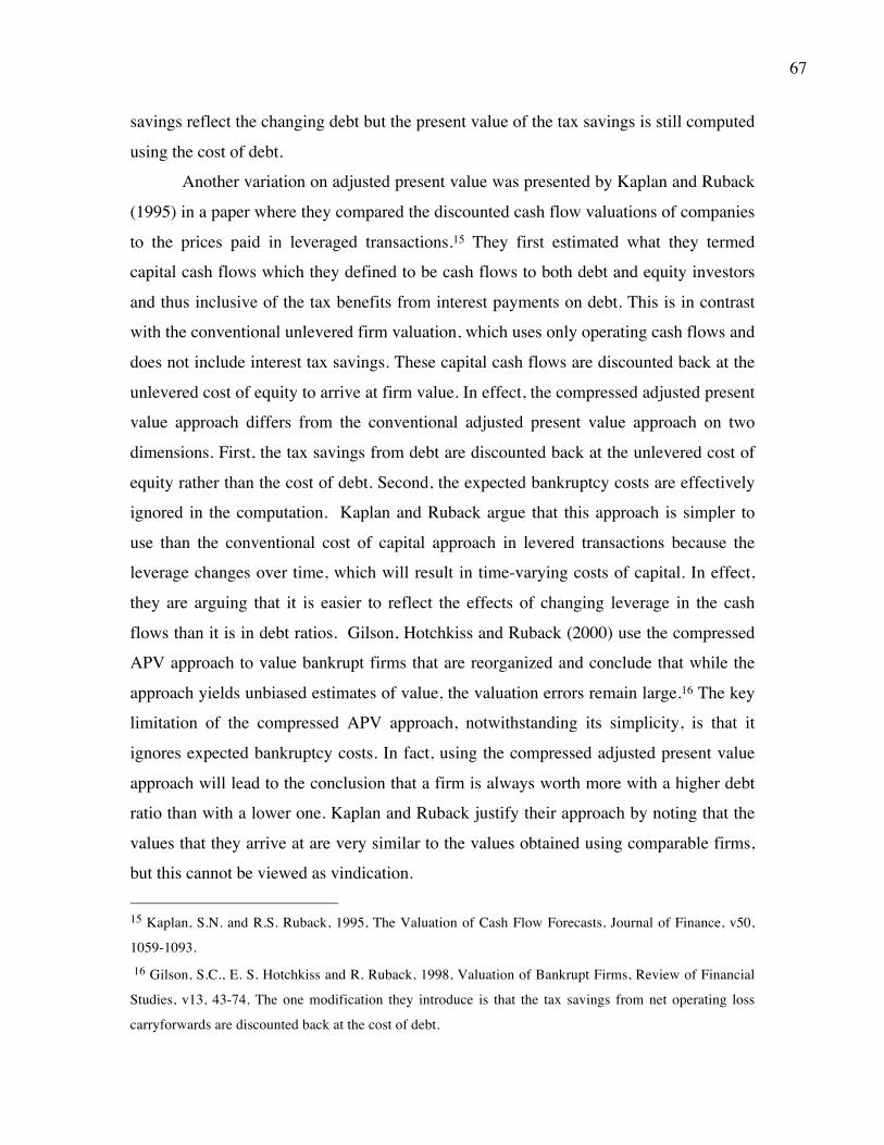
67
savings reflect the changing debt but the present value of the tax savings is still computed
using the cost of debt.
Another variation on adjusted present value was presented by Kaplan and Ruback
(1995) in a paper where they compared the discounted cash flow valuations of companies
to the prices paid in leveraged transactions.15 They first estimated what they termed
capital cash flows which they defined to be cash flows to both debt and equity investors
and thus inclusive of the tax benefits from interest payments on debt. This is in contrast
with the conventional unlevered firm valuation, which uses only operating cash flows and
does not include interest tax savings. These capital cash flows are discounted back at the
unlevered cost of equity to arrive at firm value. In effect, the compressed adjusted present
value approach differs from the conventional adjusted present value approach on two
dimensions. First, the tax savings from debt are discounted back at the unlevered cost of
equity rather than the cost of debt. Second, the expected bankruptcy costs are effectively
ignored in the computation. Kaplan and Ruback argue that this approach is simpler to
use than the conventional cost of capital approach in levered transactions because the
leverage changes over time, which will result in time-varying costs of capital. In effect,
they are arguing that it is easier to reflect the effects of changing leverage in the cash
flows than it is in debt ratios. Gilson, Hotchkiss and Ruback (2000) use the compressed
APV approach to value bankrupt firms that are reorganized and conclude that while the
approach yields unbiased estimates of value, the valuation errors remain large.16 The key
limitation of the compressed APV approach, notwithstanding its simplicity, is that it
ignores expected bankruptcy costs. In fact, using the compressed adjusted present value
approach will lead to the conclusion that a firm is always worth more with a higher debt
ratio than with a lower one. Kaplan and Ruback justify their approach by noting that the
values that they arrive at are very similar to the values obtained using comparable firms,
but this cannot be viewed as vindication. 15 Kaplan, S.N. and R.S. Ruback, 1995, The Valuation of Cash Flow Forecasts, Journal of Finance, v50,
1059-1093.
16 Gilson, S.C., E. S. Hotchkiss and R. Ruback, 1998, Valuation of Bankrupt Firms, Review of Financial
Studies, v13, 43-74. The one modification they introduce is that the tax savings from net operating loss
carryforwards are discounted back at the cost of debt.

68
Ruback (2000) provides a more extensive justification of the capital cash flow
approach to valuation.17 He notes that the conventional APV’s assumption that interest
tax savings have the same risk as the debt (and thus get discounted back at the cost of
debt) may be justifiable for a fixed dollar debt but that it is more reasonable to assume
that interest tax savings share the same risk as the operating assets, when dollar debt is
expected to change over time. He also notes that the capital cash flow approach assumes
that debt grows with firm value and is thus closer to the cost of capital approach, where
free cash flows to the firm are discounted back at a cost of capital. In fact, he shows that
when the dollar debt raised each year is such that the debt ratio stays constant, the cost of
capital approach and the capital cash flows approach yield identical results.
Cost of Capital versus APV Valuation
To understand when the cost of capital approach, the adjusted present value
approach and the modified adjusted present value approach (with capital cash flows)
yield similar and different results, we consider the mechanics of each approach in table 1:
Table 1: Cost of Capital, APV and Compressed APV
Cost of Capital Conventional APV Compressed APV Cash flow discounted
Free Cash Flow to Firm (prior to all debt payments)
Free Cash Flow to Firm (prior to debt payments)
Free Cash Flow to Firm + Tax Savings from Interest Payments
Discount Rate used Weighted average of cost of equity and after-tax cost of debt = Cost of capital
Unlevered cost of equity
Weighted average of cost of equity and pre-tax cost of debt = Unlevered cost of equity
Tax Savings from Debt
Shows up through the discount rate
Added on separately as present value of tax savings (using cost of debt as discount rate)
Shows up through cash flow
Dollar debt levels Determined by debt ratios used in cost of capital. If debt ratio
Fixed dollar debt Dollar debt can change over time – increase or decrease.
17 Ruback, R.S., 2000, Capital Cash Flows: A Simple Approach to Valuing Risky Cash Flows, Working
Paper, Harvard Business School.
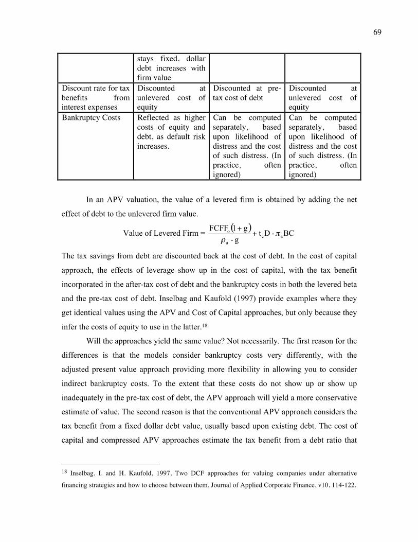
69
stays fixed, dollar debt increases with firm value
Discount rate for tax benefits from interest expenses
Discounted at unlevered cost of equity
Discounted at pre-tax cost of debt
Discounted at unlevered cost of equity
Bankruptcy Costs Reflected as higher costs of equity and debt, as default risk increases.
Can be computed separately, based upon likelihood of distress and the cost of such distress. (In practice, often ignored)
Can be computed separately, based upon likelihood of distress and the cost of such distress. (In practice, often ignored)
In an APV valuation, the value of a levered firm is obtained by adding the net
effect of debt to the unlevered firm value.
Value of Levered Firm = ( ) BC-Dtg-g1FCFF
acu
o πρ
++
The tax savings from debt are discounted back at the cost of debt. In the cost of capital
approach, the effects of leverage show up in the cost of capital, with the tax benefit
incorporated in the after-tax cost of debt and the bankruptcy costs in both the levered beta
and the pre-tax cost of debt. Inselbag and Kaufold (1997) provide examples where they
get identical values using the APV and Cost of Capital approaches, but only because they
infer the costs of equity to use in the latter.18
Will the approaches yield the same value? Not necessarily. The first reason for the
differences is that the models consider bankruptcy costs very differently, with the
adjusted present value approach providing more flexibility in allowing you to consider
indirect bankruptcy costs. To the extent that these costs do not show up or show up
inadequately in the pre-tax cost of debt, the APV approach will yield a more conservative
estimate of value. The second reason is that the conventional APV approach considers the
tax benefit from a fixed dollar debt value, usually based upon existing debt. The cost of
capital and compressed APV approaches estimate the tax benefit from a debt ratio that
18 Inselbag, I. and H. Kaufold, 1997, Two DCF approaches for valuing companies under alternative
financing strategies and how to choose between them, Journal of Applied Corporate Finance, v10, 114-122.

70
may require the firm to borrow increasing amounts in the future. For instance, assuming a
market debt to capital ratio of 30% in perpetuity for a growing firm will require it to
borrow more in the future and the tax benefit from expected future borrowings is
incorporated into value today. Finally, the discount rate used to compute the present
value of tax benefits is the pre-tax cost of debt in the conventional APV approach and the
unlevered cost of equity in the compressed APV and the cost of capital approaches. As
we noted earlier, the compressed APV approach yields equivalent values to the cost of
capital approach, if we allow dollar debt to reflect changing firm value (and debt ratio
assumptions) and ignore the effect of indirect bankruptcy costs. The conventional APV
approach yields a higher value than either of the other two approaches because it views
the tax savings from debt as less risky and assigns a higher value to it.
Which approach will yield more reasonable estimates of value? The dollar debt
assumption in the APV approach is a more conservative one but the fundamental flaw
with the APV model lies in the difficulties associated with estimating expected
bankruptcy costs. As long as that cost cannot be estimated, the APV approach will
continue to be used in half-baked form where the present value of tax benefits will be
added to the unlevered firm value to arrive at total firm value.
Conclusion In the adjusted present value approach, we separate debt from the operating assets
of the firm, and value its effects independently of the firm. The APV model is
particularly useful for levered transactions where the initial high debt level used to fund
assets is expected to decrease over time and you have access to the repayment and
interest expense schedule. It allows the analyst to first value the operating assets, without
the distraction of the heavy debt load, and to then assess the value added (or not) by the
additional debt in the transaction. Note, though, that to obtain realistic values for equity,
you have to incorporate the expected bankruptcy costs into your APV model.

71
CHAPTER 5
INTRINSIC VALUATION: EQUITY VALUATION MODELS In chapters 3 and 4, we looked at two approaches that can be used to value an
entire business or firm – discounting free cash flows to the firm at the cost of capital and
the APV approach. In this chapter, we turn our attention to an alternate way of thinking
about valuation, where we focus on valuing the equity in the firm directly, by discounting
cash flows to equity investors at the rate of return that these investors demand for
investing in the equity – the cost of equity.
Inputs to a Equity DCF Valuation In chapter 3, we outlined the key determinants to value and we reproduce the
figure below in Figure 5.1.
From the perspective of equity valuation, the first input is the cashflow from existing
assets, defined as post-debt (and to equity) earnings, net of reinvestment to generate
future growth. In fact, we can use an even stricter definition of cash flow and consider
only dividends paid. The second input is growth, with growth in equity income (net
income or earnings per share) becoming the focus when valuing equity. The third input is
the discount rate, defined as the cost of equity, since we are valuing equity. The final
input, allowing for closure, is the terminal value, defined as the estimated value of equity
at the end of the forecast period in equity valuation.
Current CashflowsThese are the cash flows from existing investment,s, net of any reinvestment needed to sustain future growth. They can be computed before debt cashflows (to the firm) or after debt cashflows (to equity investors).
Expected Growth during high growth period
Growth from new investmentsGrowth created by making new investments; function of amount and quality of investments
Efficiency GrowthGrowth generated by using existing assets better
Length of the high growth periodSince value creating growth requires excess returns, this is a function of- Magnitude of competitive advantages- Sustainability of competitive advantages
Stable growth firm, with no or very limited excess returns
Cost of financing (debt or capital) to apply to discounting cashflowsDetermined by- Operating risk of the company- Default risk of the company- Mix of debt and equity used in financing
Figure 5.1: Determinants of Value
Terminal Value of firm (equity)

72
For the rest of this section, we will focus on estimating the inputs into discounted
cash flow models, starting with the cashflows, moving on to risk (and discount rates) and
then closing with a discussion of how best to estimate the growth rate for the high growth
period and the value at the end of that period.
Cash Flows In this section, we will begin with the strictest measure of cash flow to equity, i.e.
the dividends received by investors, and then progressively move to more expansive
measures of cash flows, which generally require more information.
Dividends
When an investor buys stock, he generally expects to get two types of cash flows -
dividends during the holding period and an expected price at the end of the holding
period. Since this expected price is itself determined by future dividends, the value of a
stock is the present value of just expected dividends. If we accept this premise, the only
cash flow to equity that we should be considering in valuation is the dividend paid, and
estimating that dividend for the last period should be a simple exercise. Since many firms
do not pay dividends, this number can be zero, but it should never be negative.
Augmented Dividends
One of the limitations of focusing on dividends is that many companies,
especially in the United States but increasingly around the world, have shifted from
dividends to stock buybacks as their mechanism for returning cash to stockholders. While
only those stockholders who sell their stock back receive cash, it still represents cash
returned to equity investors. In 2007, for instance, firms in the United States returned
twice as much cash in the form of stock buybacks than they did in dividends, and
focusing only on dividends will result in the under valuation of equity. One simple way
of adjusting for this is to augment the dividend with stock buybacks and look at the
cumulative cash returned to stockholders.
Augmented Dividends = Dividends + Stock Buybacks
One problem, though, is that unlike dividends that are smoothed out over time, stock
buybacks can spike in some years and be followed by years of inaction. We therefore will

73
have to normalize buybacks by using average buybacks over a period of time (say, 5
years) to arrive at more reasonable annualized numbers.
Potential Dividends (Free Cash flow to Equity)
With both dividends and augmented dividends, we are trusting managers at
publicly traded firms to return to pay out to stockholders any excess cash left over after
meeting operating and reinvestment needs. However, we do know that managers do not
always follow this practice, as evidenced by the large cash balances that you see at most
publicly traded firms. To estimate what managers could have returned to equity investors,
we develop a measure of potential dividends that we term the free cash flow to equity.
Intuitively, the free cash flow to equity measures the cash left over after taxes,
reinvestment needs and debt cash flows have been met. It is measured as follows:
FCFE = Net Income – Reinvestment Needs – Debt Cash flows
= Net Income - (Capital Expenditures - Depreciation + Change in non-cash
working Capital – Principal) - (Repayments - New Debt Issues)
Consider the equation in pieces. We begin with net income, since that is the earnings
generated for equity investors; it is after interest expenses and taxes. We compute what
the firm has to reinvest in long term assets as net capital expenditures and what it has to
invest in short term assets as the change in non-cash working capital, thus sticking with
the definitions we attached to each term in the cost of capital model. The final input into
the process are the negative cash flows associated with the repayment of old debt and the
positive cash flows to equity investors from raising new debt. If old debt is replaced with
new debt of exactly the same magnitude, this term will be zero, but it will generate
positive (negative) cash flows when debt issues exceed (are less than) debt repayments.
Focusing on just debt cash flows allows us to zero in on a way to simplify this
computation. In the special case where the capital expenditures and the working capital
are expected to be financed at a fixed debt ratio δ, and principal repayments are made
from new debt issues, the FCFE is measured as follows:
FCFE = Net Income - (1-δ) (Capital Expenditures - Depreciation) - (1-δ) Δ Working
Capital

74
In effect, we are assuming that a firm with a 30% debt ratio that is growing through
reinvestment will choose to fund 30% of its reinvestment needs with new debt and
replace old debt that comes due with new debt.
There is one more way in which we can present the free cash flow to equity. If we
define the portion of the net income that equity investors reinvest back into the firm as
the equity reinvestment rate, we can state the FCFE as a function of this rate.
Equity Reinvestment Rate
= (Capital Expenditures - Depreciation + Δ Working Capital) (1- δ)Net Income
FCFE = Net Income (1 – Equity Reinvestment Rate)
A final note on the contrast between the first two measures of cash flows to equity
(dividends and augmented dividends) and this measure. Unlike those measures, which
can never be less than zero, the free cash flow to equity can be negative for a number of
reasons. The first is that the net income could be negative, a not uncommon phenomenon
even for mature firms. The second is that reinvestment needs can overwhelm net income,
which is often the case for growth companies, especially early in the life cycle. The third
is that large debt repayments coming due that have to funded with equity cash flows can
cause negative FCFE; highly levered firms that are trying to bring their debt ratios down
can go through years of negative FCFE. The fourth is that the quirks of the reinvestment
process, where firms invest large amounts in long-lived and short-lived assets in some
years and nothing in others, can cause the FCFE to be negative in the big reinvestment
years and positive in others. As with buybacks, we have to consider normalizing
reinvestment numbers across time when estimating cash flows to equity. If the FCFE is
negative, it is indicative of the firm needing to raise fresh equity.
Risk and Discount Rates In chapter 3, we laid out the core issues in estimating the cost of equity. We noted
first the difficult in estimating an implicit cost (cost of equity is implicit whereas the
interest rate on a loan is explicit) and argued that we should estimate the cost of equity
through the eyes of the marginal investor in the company. In fact, if that marginal
investor is diversified, the risk that we measure is only the risk that cannot be diversified

75
away. We also looked at the different models for estimating cost of equity (the CAPM,
the Arbitrage Pricing Model and Multi-factor Models) and the challenges in estimating
the inputs to these models.
We would like to add a couple of intuitive points to that discussion. The first is
that the cost of equity for a firm can and often should change over time, as its growth rate
changes and it approaches maturity. Using beta as a measure for growth, for instance, you
would expect to see the beta for a young, growth firm go from 1.80 today (when it is
young, high growth and risky) to a number closer to one as the firm approaches maturity.
The second is to reemphasize a point we made in the earlier chapter on estimating betas.
It is bad practice to trust a single regression (or a service that reports that regression) for
the beta for your company. You will be better served using industry averages for the
businesses in which your firm operates and correcting for financial and operating
leverage differences.
Growth Rates
To estimate growth rates in equity earnings, we can draw on some of the same
approaches we used for operating earnings, looking at historical growth or trusting in
analyst forecasts, but they are just as flawed in this context as they were in the operating
income context. Consequently, we will fall back on the same approach that we focused
on for operating income, which is to link expected growth in earnings to how much a
firm reinvests and how well it does so.
While investment and return on investment are generic terms, the way in which
we define them will depend upon whether we are looking at equity earnings or operating
income. When looking at equity earnings, our focus is on the investment in equity and the
return is the return on equity. The change in investment is computed as the reinvestment,
with the measurement of the reinvestment again varying depending upon the cash flow
being discounted. In dividend discount models, reinvestment is defined as retained
earnings (i.e.. any income not paid out as dividends). In free cash flow to equity (firm)
models, reinvestment is defined in terms of the equity reinvestment rate (reinvestment
rate).
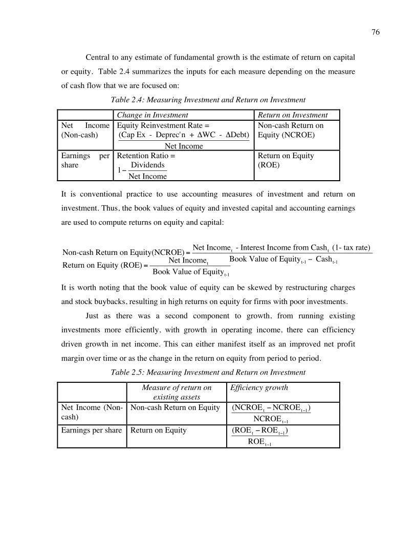
76
Central to any estimate of fundamental growth is the estimate of return on capital
or equity. Table 2.4 summarizes the inputs for each measure depending on the measure
of cash flow that we are focused on:
Table 2.4: Measuring Investment and Return on Investment
Change in Investment Return on Investment Net Income (Non-cash)
Equity Reinvestment Rate =
€
(Cap Ex - Deprec'n + ΔWC - ΔDebt)Net Income
Non-cash Return on Equity (NCROE)
Earnings per share
Retention Ratio =
€
1− DividendsNet Income
Return on Equity (ROE)
It is conventional practice to use accounting measures of investment and return on
investment. Thus, the book values of equity and invested capital and accounting earnings
are used to compute returns on equity and capital:
Non-cash Return on Equity(NCROE) = Net Incomet - Interest Income from Casht (1- tax rate) Book Value of Equityt-1 − Casht-1Return on Equity (ROE) = Net Incomet
Book Value of Equityt-1
It is worth noting that the book value of equity can be skewed by restructuring charges
and stock buybacks, resulting in high returns on equity for firms with poor investments.
Just as there was a second component to growth, from running existing
investments more efficiently, with growth in operating income, there can efficiency
driven growth in net income. This can either manifest itself as an improved net profit
margin over time or as the change in the return on equity from period to period.
Table 2.5: Measuring Investment and Return on Investment
Measure of return on existing assets
Efficiency growth
Net Income (Non-cash)
Non-cash Return on Equity
€
(NCROEt −NCROEt−1)NCROEt−1
Earnings per share Return on Equity
€
(ROEt −ROEt−1)ROEt−1

77
Terminal Value
When discussing terminal value in the context of the cost of capital approach, we
noted three key constraints: (a) Make sure that the growth rate you estimate in perpetuity
is less than the growth rate of the economy. In fact, we suggested using the riskfree rate
as a proxy for long term growth in the economy and setting the growth rate at or below
the riskfee rate (b) Give the company the characteristics of a mature company in stable
growth. In the context of equity models, this requires us to bring the beta of the company
closer to one, the beta for the market and (c) Make sure you reinvest to sustain the stable
growth rate.
Stable growth firms tend to reinvest less than high growth firms and it is critical
that we both capture the effects of lower growth on reinvestment and that we ensure that
the firm reinvests enough to sustain its stable growth rate in the terminal phase. Given the
relationship between growth, reinvestment rate and returns that we established in the
section on expected growth rates, we can estimate the reinvestment rate that is consistent
with expected growth in table 2.7:
Table 2.7: Reinvestment in Stable Growth
Model Reinvestment Rate in stable growth
Dividend
€
Stable Growth rateReturn on Equity in stable growth
FCFE
€
Stable Growth rateNon - cash Return on Equity in stable growth
Linking the equity reinvestment rate and retention ratio to the stable growth rate
also makes the valuation less sensitive to assumptions about stable growth. While
increasing the stable growth rate, holding all else constant, can dramatically increase
value, changing the reinvestment rate as the growth rate changes will create an offsetting
effect.
€
Terminal Value of Equity = Net Incomen +1 1- gn
ROE n
"
# $
%
& '
(Cost of Equityn − gn )

78
In the special case where the cost of equity = ROE, the growth rate becomes irrelevant
and the terminal value of equity can be written as:
€
Terminal ValueROE=Cost of Equity = Net Incomen +1 Cost of Equityn
Tying up loose ends When using equity valuation models, there are fewer loose ends to tie up, partly
because net income already includes the income from cash and cross holdings but that I
always not a hard and fast rule. Thus, if the cash flows are based non-cash net income, we
have not valued cash yet and it should be added on to the present value. If, on the other
hand, we estimate cash flows from the cumulative net income or use the dividend
discount model, cash already has been implicitly valued; the income from cash is part of
the final cash flow and the discount rate presumably has been adjusted to reflect the
presence of cash.
There is no need to net debt out, since we have estimated the equity value in the
business, though we may still net out underfunded pension/health care obligations or the
costs of a potential lawsuit from the equity value. We should still subtract out the
estimated value of employee options, since that represents a drain on equity value to
common shareholders. Table 5.3 summarizes how we deal with loose ends in different
discounted cash flow models.
Table 2.9: Dealing with loose ends in valuation
Loose End Dividend Discount Model
FCFE Model FCFF Model
Cash and Marketable Securities
Ignore, since net income includes interest income from cash.
Ignore, if FCFE is computed using total net income. Add, if FCFE is computed using non-cash net income
Add. Operating income does not include income from cash.
Cross Holdings Ignore, since net income includes income from cross holdings.
Ignore, since net income includes income from cross holdings.
Add market value of minority holdings and subtract market value of minority interests.
Other Liabilities Ignore. The Subtract out expected Subtract out under

79
assumption is that the firm is considering costs when setting dividends.
litigation costs. funded pension obligations, health care obligations and expected litigation costs.
Employee options
Ignore. Subtract out value of equity options outstanding
Subtract out value of equity options outstanding
FCFE versus Dividend Discount Model Valuation
The FCFE model can be viewed as an alternative to the dividend discount model.
Since the two approaches sometimes provide different estimates of value for equity, it is
worth examining when they provide similar estimates of value, when they provide
different estimates of value and what the difference tells us about the firm.
a. When they are similar
There are two conditions under which the value from using the FCFE in
discounted cashflow valuation will be the same as the value obtained from using the
dividend discount model. The first is the obvious one, where the dividends are equal to
the FCFE. There are firms that maintain a policy of paying out excess cash as dividends
either because they have pre-committed to doing so or because they have investors who
expect this policy of them.
The second condition is more subtle, where the FCFE is greater than dividends,
but the excess cash (FCFE - Dividends) is invested in fairly priced assets (i.e. assets that
earn a fair rate of return and thus have zero net present value). For instance, investing in
financial assets that are fairly priced should yield a net present value of zero. To get
equivalent values from the two approaches, though, we have to keep track of
accumulating cash in the dividend discount model and add it to the value of equity (as
shown in illustration 5.10 at the end of this section).
b. When they are different
There are several cases where the two models will provide different estimates of
value. First, when the FCFE is greater than the dividend and the excess cash either earns

80
below-market interest rates or is invested in negative net present value assets, the value
from the FCFE model will be greater than the value from the dividend discount model.
There is reason to believe that this is not as unusual as it would seem at the outset. There
are numerous case studies of firms, which having accumulated large cash balances by
paying out low dividends relative to FCFE, have chosen to use this cash to finance
unwise takeovers (where the price paid is greater than the value received from the
takeover). Second, the payment of dividends less than FCFE lowers debt-equity ratios
and may lead the firm to become under levered, causing a loss in value.
In the cases where dividends are greater than FCFE, the firm will have to issue
either new stock or debt to pay these dividends or cut back on its investments, leading to
at least one of three negative consequences for value. If the firm issues new equity to
fund dividends, it will face substantial issuance costs that decrease value. If the firm
borrows the money to pay the dividends, the firm may become over levered (relative to
the optimal) leading to a loss in value. Finally, if paying too much in dividends leads to
capital rationing constraints where good projects are rejected, there will be a loss of value
(captured by the net present value of the rejected projects).
There is a third possibility and it reflects different assumptions about reinvestment
and growth in the two models. If the same growth rate used in the dividend discount and
FCFE models, the FCFE model will give a higher value than the dividend discount model
whenever FCFE are higher than dividends and a lower value when dividends exceed
FCFE. In reality, the growth rate in FCFE should be different from the growth rate in
dividends, because the free cash flow to equity is assumed to be paid out to stockholders.
This will affect the equity reinvestment rate of the firm. In addition, the return on equity
used in the FCFE model should reflect the return on equity on non-cash investments,
whereas the return on equity used in the dividend discount model should be the overall
return on equity. In general, when firms pay out much less in dividends than they have
available in FCFE, the expected growth rate and terminal value will be higher in the
dividend discount model, but the year-to-year cash flows will be higher in the FCFE
model.

81
3. What does it mean when they are different?
When the value using the FCFE model is different from the value using the
dividend discount model, with consistent growth assumptions, there are two questions
that need to be addressed - What does the difference between the two models tell us?
Which of the two models is the appropriate one to use in evaluating the market price?
The more common occurrence is for the value from the FCFE model to exceed
the value from the dividend discount model. The difference between the value from the
FCFE model and the value using the dividend discount model can be considered one
component of the value of controlling a firm - it measures the value of controlling
dividend policy. In a hostile takeover, the bidder can expect to control the firm and
change the dividend policy (to reflect FCFE), thus capturing the higher FCFE value.
As for which of the two values is the more appropriate one for use in evaluating
the market price, the answer lies in the openness of the market for corporate control. If
there is a sizable probability that a firm can be taken over or its management changed, the
market price will reflect that likelihood and the appropriate benchmark to use is the value
from the FCFE model. As changes in corporate control become more difficult, either
because of a firm's size and/or legal or market restrictions on takeovers, the value from
the dividend discount model will provide the appropriate benchmark for comparison.
Per Share versus Aggregate Valuation In this chapter, some of the valuations that we did used per share values for
earnings and cash flows and arrived at a per share estimate of value for equity. Other
valuations used aggregate net income and cash flows and arrived at the aggregate value
for equity. Why use one approach over the other and what are the pros and cons?
The per share approach tends to be a little simpler and information is usually more
accessible. Most data services report earnings per share and analyst estimates of growth
in earnings per share. There are two reasons, though, for sticking with aggregate
valuation. The first is that it is easier to keep operating assets separate from cash, if we
begin with net income rather than earnings per share, and break it down into net income
from operating assets and cash income. The second is that the number of shares to use to
compute per share values can be subject to debate when there are options, warrants and
82
convertible bonds outstanding. These equity options issued by the firm can be converted
into shares, thus altering the number of shares outstanding. Analysts do try to factor in
these options by computing the partially diluted (where options in the money are counted
as shares outstanding) or fully diluted (where all options are counted) per share values.
However, options do not lend themselves easily to this characterization. A much more
robust way of dealing with options is to value them as options and to subtract this value
from the aggregate value of equity estimated for a firm to arrive at an equity value for
common stock. Dividing this value by the actual number of shares outstanding should
yield the correct value for equity per share. We will deal with this question much more
extensively later in this book, when we look at employee stock options and their effects
on value.
Firm valuation versus equity valuation The equity valuation models, whether they use dividends or free cash flows to
equity, yield a value for the equity in a company. The value of equity, however, can be
extracted from the value of the firm by subtracting out the market value of outstanding
debt. Since these are alternative ways of valuing equity, two questions arise - Why value
the firm rather than equity? Will the values for equity obtained from the firm valuation
approach be consistent with the values obtained from the equity valuation approaches?
The advantage of using the firm valuation approach is that cashflows relating to
debt do not have to be considered explicitly, since the FCFF is a pre-debt cashflow, while
they have to be taken into account in estimating FCFE. In cases where the leverage is
expected to change significantly over time, this is a significant saving, since estimating
new debt issues and debt repayments when leverage is changing can become increasingly
messy the further into the future you go. The firm valuation approach does, however,
require information about debt ratios and interest rates to estimate the weighted average
cost of capital.
The value for equity obtained from the firm valuation and equity valuation
approaches will be the same if you make consistent assumptions about financial leverage.
Getting them to converge in practice is much more difficult. Let us begin with the
simplest case – a no-growth, perpetual firm. Assume that the firm has $166.67 million in

83
earnings before interest and taxes and a tax rate of 40%. Assume that the firm has equity
with a market value of $600 million, with a cost of equity of 13.87% debt of $400 million
and with a pre-tax cost of debt of 7%. The firm’s cost of capital can be estimated.
Cost of capital = ( ) ( )( ) 10%10004000.4-17%
100060013.87% =!
"
#$%
&+!"
#$%
&
Value of the firm = ( ) ( ) $1,0000.10
0.4-1166.67capital ofCost
t-1EBIT==
Note that the firm has no reinvestment and no growth. We can value equity in this firm
by subtracting out the value of debt.
Value of equity = Value of firm – Value of debt = $ 1,000 - $400 = $ 600 million
Now let us value the equity directly by estimating the net income:
Net Income = (EBIT – Pre-tax cost of debt * Debt) (1-t) = (166.67 - 0.07*400) (1-0.4) =
83.202 million
The value of equity can be obtained by discounting this net income at the cost of equity:
Value of equity = million 600 $0.138783.202
equity ofCost IncomeNet
==
Even this simple example works because of the following assumptions that we made
implicitly or explicitly during the valuation.
1. The values for debt and equity used to compute the cost of capital were equal to
the values that we obtained in the valuation. Notwithstanding the circularity in
reasoning – you need the cost of capital to obtain the values in the first place – it
indicates that a cost of capital based upon market value weights will not yield the
same value for equity as an equity valuation model, if the firm is not fairly priced
in the first place.
2. There are no extraordinary or non-operating items that affect net income but not
operating income. Thus, to get from operating to net income, all we do is subtract
out interest expenses and taxes.
3. The interest expenses are equal to the pre-tax cost of debt multiplied by the
market value of debt. If a firm has old debt on its books, with interest expenses
that are different from this value, the two approaches will diverge.

84
If there is expected growth, the potential for inconsistency multiplies. You have to ensure
that you borrow enough money to fund new investments to keep your debt ratio at a level
consistent with what you are assuming when you compute the cost of capital.
Conclusion The intrinsic value of a company reflects its fundamentals. The primary tool for
estimating intrinsic value is the discounted cash flow model. We started by looking at the
contrast between valuing the equity in a business and valuing the entire business, and
then moved on to the four inputs that we need for the model. The cash flows to equity
investors can be defined strictly as dividends, more expansively as dividends augmented
with stock buybacks and most generally as free cash flows to equity (potential dividends).
The cash flow to the firm is the cumulative cash flow to both equity investors and
lenders, and thus is a pre-debt cash flow. The discount rates we apply have to be
consistent with the cash flow definition, with the cost of equity used to discount cash
flows to equity and the cost of capital to discount cash flows to the firm. When estimating
growth, we noted the limitations of historical growth numbers and outside estimates, and
the importance of linking growth to fundamentals. Finally, we applied closure to the
models by assuming that cash flows will settle into stable growth, sometime in the future,
but imposed constraints on what this growth rate can be and the characteristics of stable
growth companies.
We closed the chapter by looking at three variations on the discounted cash flow
model. In the certainty equivalent approach, we adjusted the cash flows for risk and
discounted back at the riskfree rate. In the adjusted present value approach, we separated
debt from the operating assets of the firm, and valued its effects independently of the
firm. In the excess return model, we zeroed in on the fact that its is not growth per se that
creates value but growth with excess returns. However, we noted that the models agree at
the core, though there are minor differences in assumptions.
85
CHAPTER 6
RELATIVE VALUATION In discounted cash flow valuation, the objective is to find the value of an asset,
given its cash flow, growth and risk characteristics. In relative valuation, the objective is
to value an asset, based upon how similar assets are currently priced by the market.
Consequently, there are two components to relative valuation. The first is that to value
assets on a relative basis, prices have to be standardized, usually by converting prices into
multiples of some common variable. While this common variable will vary across assets,
it usually takes the form of earnings, book value or revenues for publicly traded stocks..
The second is to find similar assets, which is difficult to do since no two assets are
exactly identical. With real assets like antiques and baseball cards, the differences may be
small and easily controlled for when pricing the assets. In the context of valuing equity in
firms, the problems are compounded since firms in the same business can still differ on
risk, growth potential and cash flows. The question of how to control for these
differences, when comparing a multiple across several firms, becomes a key one.
While relative valuation is easy to use and intuitive, it is also easy to misuse. In
this chapter, we will develop a four-step process for doing relative valuation. In the
process, we will also develop a series of tests that can be used to ensure that multiples are
correctly used.
What is relative valuation? In relative valuation, we value an asset based upon how similar assets are priced
in the market. A prospective house buyer decides how much to pay for a house by
looking at the prices paid for similar houses in the neighborhood. A baseball card
collector makes a judgment on how much to pay for a Mickey Mantle rookie card by
checking transactions prices on other Mickey Mantle rookie cards. In the same vein, a
potential investor in a stock tries to estimate its value by looking at the market pricing of
“similar” stocks.
Embedded in this description are the three essential steps in relative valuation.
The first step is finding comparable assets that are priced by the market, a task that is

86
easier to accomplish with real assets like baseball cards and houses than it is with stocks.
All too often, analysts use other companies in the same sector as comparable, comparing
a software firm to other software firms or a utility to other utilities. The second step is
scaling the market prices to a common variable to generate standardized prices that are
comparable. While this may not be necessary when comparing identical assets (Mickey
Mantle rookie cards), it is necessary when comparing assets that vary in size or units.
Other things remaining equal, a smaller house or apartment should trade at a lower price
than a larger residence. In the context of stocks, this equalization usually requires
converting the market value of equity or the firm into multiples of earnings, book value
or revenues. The third and last step in the process is adjusting for differences across
assets when comparing their standardized values. Again, using the example of a house, a
newer house with more updated amenities should be priced higher than a similar sized
older house that needs renovation. With stocks, differences in pricing across stocks can
be attributed to all of the fundamentals that we talked about in discounted cash flow
valuation. Higher growth companies, for instance, should trade at higher multiples than
lower growth companies in the same sector. Many analysts adjust for these differences
qualitatively, making every relative valuation a story telling experience; analysts with
better and more believable stories are given credit for better valuations.
There is a significant philosophical difference between discounted cash flow and
relative valuation. In discounted cash flow valuation, we are attempting to estimate the
intrinsic value of an asset based upon its capacity to generate cash flows in the future. In
relative valuation, we are making a judgment on how much an asset is worth by looking
at what the market is paying for similar assets. If the market is correct, on average, in the
way it prices assets, discounted cash flow and relative valuations may converge. If,
however, the market is systematically over pricing or under pricing a group of assets or
an entire sector, discounted cash flow valuations can deviate from relative valuations.
Standardized Values and Multiples Comparing assets that are not exactly similar can be a challenge. If we have to
compare the prices of two buildings of different sizes in the same location, the smaller
building will look cheaper unless we control for the size difference by computing the

87
price per square foot. When comparing publicly traded stocks across companies, the
price per share of a stock is a function both of the value of the equity in a company and
the number of shares outstanding in the firm. To compare the values of “similar” firms in
the market, we need to standardize the values in some way by scaling them to a common
variable. In general, values can be standardized relative to the earnings firms generate, to
the books values, to the revenues that firms generate or to measures that are specific to
firms in a sector. Figure 6.1 lists the alternatives:
Figure 6.1: Choices in Standardization
To provide a couple of illustrations, we can divide the market value of equity by the net
income to estimate the PE ratio (measuring how much equity investors are paying per
dollar of earnings), or the enterprise value to EBITDA to get a sense of the market value
of operating assets, relative to operating cash flows. We can even estimate what we are
paying as a market value per subscriber in a cable company or what the market value is
relative to the accounting estimate of value (book value). The central reason for
standardizing, though, does not change. We want to compare these numbers across
companies.
The Four Basic Steps to Using Multiples Multiples are easy to use and easy to misuse. There are four basic steps to using
multiples wisely and for detecting misuse in the hands of others. The first step is to
ensure that the multiple is defined consistently and that it is measured uniformly across
the firms being compared. The second step is to be aware of the cross sectional
Numerator = What you are paying for the asset
Denominator = What you are getting in return
Market value of equity Market value for the firmFirm value = Market value of equity
+ Market value of debt
Market value of operating assets of firmEnterprise value (EV) = Market value of equity
+ Market value of debt- Cash
Revenuesa. Accounting revenuesb. Drivers- # Customers- # Subscribers- # units
Earningsa. To Equity investors - Net Income - Earnings per shareb. To Firm - Operating income (EBIT)
Book Valuea. Equity= BV of equityb. Firm= BV of debt + BV of equityc. Invested Capital= BV of equity + BV of debt - Cash
Multiple =
Cash flowa. To Equity- Net Income + Depreciation- Free CF to Equityb. To Firm- EBIT + DA (EBITDA)- Free CF to Firm
88
distribution of the multiple, not only across firms in the sector being analyzed but also
across the entire market. The third step is to analyze the multiple and understand not only
what fundamentals determine the multiple but also how changes in these fundamentals
translate into changes in the multiple. The final step is finding the right firms to use for
comparison and controlling for differences that may persist across these firms.
1. Definitional Tests
Even the simplest multiples are defined differently by different analysts.
Consider, for instance, the price earnings ratio (PE), the most widely used valuation
multiple in valuation. Analysts define it to be the market price divided by the earnings per
share but that is where the consensus ends. There are a number of variants on the PE
ratio. While the current price is conventionally used in the numerator, there are some
analysts who use the average price over the last six months or a year. The earnings per
share in the denominator can be the earnings per share from the most recent financial
year (yielding the current PE), the last four quarters of earnings (yielding the trailing PE)
and expected earnings per share in the next financial year (resulting in a forward PE). In
addition, earnings per share can be computed based upon primary shares outstanding or
fully diluted shares and can include or exclude extraordinary items.
Not only can these variants on earnings yield vastly different values for the price
earnings ratio but the one that gets used by analysts depends upon their biases. For
instance, in periods of rising earnings, the forward PE will yield consistently lower values
than the trailing PE, which, in turn, will be lower than the current PE. A bullish analyst
will tend to use the forward PE to make the case that the stock is trading at a low multiple
of earnings, while a bearish analyst will focus on the current PE to make the case that the
multiple is too high. The first step when discussing a valuation based upon a multiple is
to ensure that everyone in the discussion is using the same definition for that multiple.
Consistency
Every multiple has a numerator and a denominator. The numerator can be either
an equity value (such as market price or value of equity) or a firm value (such as
enterprise value, which is the sum of the values of debt and equity, net of cash). The
denominator can be an equity measure (such as earnings per share, net income or book
89
value of equity) or a firm measure (such as operating income, EBITDA or book value of
capital).
One of the key tests to run on a multiple is to examine whether the numerator and
denominator are defined consistently. If the numerator for a multiple is an equity value,
then the denominator should be an equity value as well. If the numerator is a firm value,
then the denominator should be a firm value as well. To illustrate, the price earnings ratio
is a consistently defined multiple, since the numerator is the price per share (which is an
equity value) and the denominator is earnings per share (which is also an equity value).
So is the Enterprise value to EBITDA multiple, since the numerator and denominator are
both firm value measures; the enterprise value measures the market value of the operating
assets of a company and the EBITDA is the cashflow generated by the operating assets,
prior to taxes and reinvestment needs.
Are there any multiples in use that are inconsistently defined? Consider the price
to EBITDA multiple, a multiple that has acquired adherents in the last few years among
analysts. The numerator in this multiple is an equity value and the denominator is a
measure of earnings to the firm. The analysts who use this multiple will probably argue
that the inconsistency does not matter since the multiple is computed the same way for all
of the comparable firms; but they would be wrong. If some firms on the list have no debt
and others carry significant amounts of debt, the latter will look cheap on a price to
EBITDA basis, when in fact they might be over or correctly priced.
Uniformity
In relative valuation, the multiple is computed for all of the firms in a group and
then compared across these firms to make judgments on which firms are over priced and
which are under priced. For this comparison to have any merit, the multiple has to be
defined uniformly across all of the firms in the group. Thus, if the trailing PE is used for
one firm, it has to be used for all of the others as well. In fact, one of the problems with
using the current PE to compare firms in a group is that different firms can have different
fiscal-year ends. This can lead to some firms having their prices divided by earnings from
July 2007 to June 2008, with other firms having their prices divided by earnings from
January 2008 to December 2008. While the differences can be minor in mature sectors,

90
where earnings do not make quantum jumps over six months, they can be large in high-
growth sectors.
With both earnings and book value measures, there is another component to be
concerned about and that is the accounting standards used to estimate earnings and book
values. Differences in accounting standards can result in very different earnings and book
value numbers for similar firms. This makes comparisons of multiples across firms in
different markets, with different accounting standards, very difficult. Even with the same
accounting standards governing companies, there can be differences in firms that arise
because of discretionary accounting choices. There is also the additional problem posed
by the fact that some firms use different accounting rules (on depreciation and expensing)
for reporting purposes and tax purposes and others do not.19 In summary, companies that
use aggressive assumptions in measuring earnings will look cheaper on earnings
multiples than firms that adopt conservative accounting practices.
2. Descriptive Tests
When using a multiple, it is always useful to have a sense of what a high value, a low
value or a typical value for that multiple is in the market. In other words, knowing the
distributional characteristics of a multiple is a key part of using that multiple to identify
under or over valued firms. In addition, we need to understand the effects of outliers on
averages and unearth any biases in these estimates, introduced in the process of
estimating multiples. In the final part of this section, we will look at how the distributions
of multiples shift over time.
Distributional Characteristics
When using multiples to value companies, we often compare the values across
companies in a sector. What is often lacking, however, is a sense of how the multiple is
distributed across the entire market. The standard statistics – the average and standard
deviation – are where we should start, but they represent the beginning of the exploration.
19 Firms that adopt different rules for reporting and tax purposes generally report higher earnings to their
stockholders than they do to the tax authorities. When they are compared on a price earnings basis to firms
that do not maintain different reporting and tax books, they will look cheaper (lower PE).
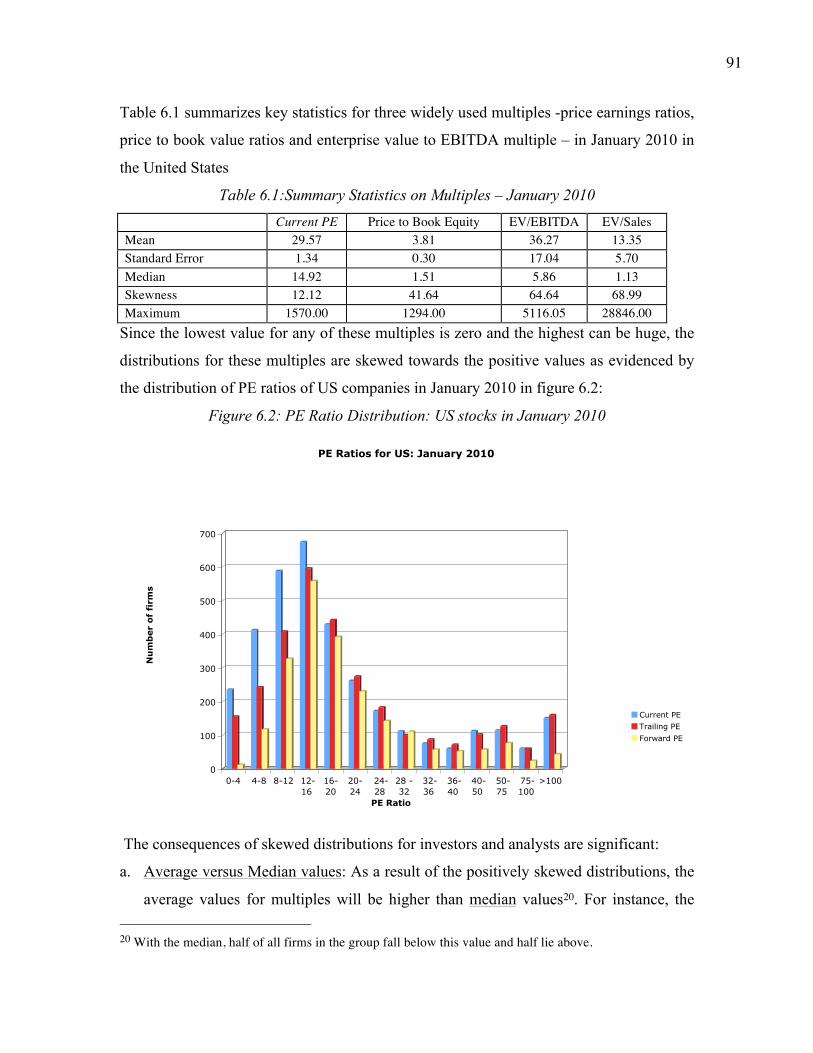
91
Table 6.1 summarizes key statistics for three widely used multiples -price earnings ratios,
price to book value ratios and enterprise value to EBITDA multiple – in January 2010 in
the United States
Table 6.1:Summary Statistics on Multiples – January 2010 Current PE Price to Book Equity EV/EBITDA EV/Sales
Mean 29.57 3.81 36.27 13.35 Standard Error 1.34 0.30 17.04 5.70 Median 14.92 1.51 5.86 1.13 Skewness 12.12 41.64 64.64 68.99 Maximum 1570.00 1294.00 5116.05 28846.00
Since the lowest value for any of these multiples is zero and the highest can be huge, the
distributions for these multiples are skewed towards the positive values as evidenced by
the distribution of PE ratios of US companies in January 2010 in figure 6.2:
Figure 6.2: PE Ratio Distribution: US stocks in January 2010
The consequences of skewed distributions for investors and analysts are significant:
a. Average versus Median values: As a result of the positively skewed distributions, the
average values for multiples will be higher than median values20. For instance, the 20 With the median, half of all firms in the group fall below this value and half lie above.
0
100
200
300
400
500
600
700
Nu
mb
er
of
firm
s
0-4 4-8 8-12 12-16
16-20
20-24
24-28
28 -32
32-36
36-40
40-50
50-75
75-100
>100
PE Ratio
PE Ratios for US: January 2010
Current PETrailing PEForward PE

92
median PE ratio in January 2010 was about 15, well below the average PE reported in
table 4.1 and this is true for all multiples. The median value is much more
representative of the typical firm in the group and any comparisons should be made to
medians. The standard sales pitch of a stock being cheap because it trades at a
multiple less than the average for the sector should be retired in favor of one which
compares the stock’s pricing to the median for the sector.
b. Probabilistic statements: As a result of the focus on normal distributions in most
statistics classes, we begin attributing its properties to all distributions. For instance, it
is true that the probability of values in a normal distribution falling more than two
standard deviations away from the mean is very small. In the case of the PE ratio, this
rule would suggest that few companies should have PE ratios that fall below 27.89
(which is the average of 29.57 minus two standard errors) or above 32.25 (the average
plus two standard errors). The reality is that there are thousands of firms that fall
outside this range because the distributions are not normal.
c. Outliers and averages: Since multiples can take on extreme values, data reporting
services that compute and report average values for multiples either throw out these
outliers when computing the averages or constrain the multiples to be less than or
equal to a fixed number. For instance, any firm that has a price earnings ratio greater
than 500 will be assumed to have a price earnings ratio of 500. The consequence is
that the averages reported by two services for the same sector or market will almost
never match up because they deal with outliers differently.
Analytical Tests
In discussing why analysts were so fond of using multiples, we argued that relative
valuations require fewer assumptions than discounted cash flow valuations. While this is
technically true, it is only so on the surface. In reality, we make just as many assumptions
when we do a relative valuation as we do in a discounted cash flow valuation. The
difference is that the assumptions in a relative valuation are implicit and unstated,
whereas those in discounted cash flow valuation are explicit and stated. The two primary
questions that we need to answer before using a multiple are: What are the fundamentals

93
that determine at what multiple a firm should trade? How do changes in the fundamentals
affect the multiple?
Determinants
In the introduction to discounted cash flow valuation, we observed that the value
of a firm is a function of three variables – it’s capacity to generate cash flows, its
expected growth in these cash flows and the uncertainty associated with these cash flows.
Every multiple, whether it is of earnings, revenues or book value, is a function of the
same three variables – risk, growth and cash flow generating potential. Intuitively, then,
firms with higher growth rates, less risk and greater cash flow generating potential should
trade at higher multiples than firms with lower growth, higher risk and less cash flow
potential.
The specific measures of growth, risk and cash flow generating potential that are
used will vary from multiple to multiple. To look under the hood, so to speak, of equity
and firm value multiples, we can go back to fairly simple discounted cash flow models
for equity and firm value and use them to derive the multiples.
In the simplest discounted cash flow model for equity, which is a stable growth
dividend discount model, the value of equity is:
Value of Equity =
€
P0 =DPS1k e − gn
where DPS1 is the expected dividend in the next year, ke is the cost of equity and gn is the
expected stable growth rate. Dividing both sides by the earnings, we obtain the
discounted cash flow equation specifying the PE ratio for a stable growth firm.
€
P0EPS0
= PE = Payout Ratio* (1+ gn )
ke-gn
The key determinants of the PE ratio are the expected growth rate in earnings per share,
the cost of equity and the payout ratio. Other things remaining equal, we would expect
higher growth, lower risk and higher payout ratio firms to trade at higher multiples of
earnings than firms without these characteristics.
Dividing both sides by the book value of equity, we can estimate the price/book
value ratio for a stable growth firm.
94
€
P0BV0
= PBV = ROE * Payout Ratio* (1+ gn )
k e-gn
where ROE is the return on equity and is the only variable in addition to the three that
determine PE ratios (growth rate, cost of equity and payout) that affects price to book
equity.
Dividing by the Sales per share, the price/sales ratio for a stable growth firm can
be estimated as a function of its profit margin, payout ratio, risk and expected growth.
€
P0Sales0
= PS = Profit Margin * Payout Ratio* (1+ gn )
ke-gn
The net margin is the new variable that is added to the process. While all of these
computations are based upon a stable growth dividend discount model, we will show that
the conclusions hold even when we look at companies with high growth potential and
with other equity valuation models.
We can do a similar analysis to derive the firm value multiples. The value of a
firm in stable growth can be written as:
Value of Firm =
€
V0 =FCFF1k c − gn
Dividing both sides by the expected free cash flow to the firm yields the Value/FCFF
multiple for a stable growth firm.
€
V0FCFF1
=1
k c − gn
The multiple of FCFF that a firm commands will depend upon two variables – its cost of
capital and its expected stable growth rate. Since the free cash flow the firm is the after-
tax operating income netted against the net capital expenditures and working capital
needs of the firm, the multiples of revenues, EBIT and after-tax EBIT can also be
estimated similarly.
€
V0
EBIT1(1− t)=
(1- Reinvestment Rate) k c − gn

95
€
V0
EBIT1
=(1- Reinvestment Rate)(1- t)
k c − gn
€
V0
Sales=
After - tax Operating Margin (1- Reinvestment Rate) k c − gn
Table 6.2 summarizes the multiples and the key variables that determine each multiple,
with the sign of the relationship in brackets next to each variable: ñ indicates that an
increase in this variable will increase the multiple, whereas ê indicates that an increase
in this variable will decrease the multiple, holding all else constant.
Table 6.2: Fundamentals Determining Multiples
Multiple Fundamental Determinants
Price Earnings Ratio Expected Growth(ñ), Payout(ñ), Risk(ê)
Price to Book Equity Ratio Expected Growth(ñ), Payout(ñ), Risk(ê), ROE(ñ)
Price to Sales Ratio Expected Growth(ñ), Payout(ñ), Risk(ê), Net
Margin(ñ)
EV to FCFF Cost of capital(ê), Growth Rate(ñ)
EV to EBITDA Expected Growth(ñ), Reinvestment Rate(ê), Risk(ê),
ROC(ñ), Tax rate(ê)
EV to Capital Ratio Expected Growth(ñ), Reinvestment Rate(ê), Risk(ê),
ROC(ñ)
EV to Sales Expected Growth(ñ), Reinvestment Rate(ê), Risk(ê),
Operating Margin(ñ)
The point of this analysis is not to suggest that we go back to using discounted cash flow
valuation, but to understand the variables that may cause these multiples to vary across
firms in the same sector. If we ignore these variables, we might conclude that a stock
with a PE of 8 is cheaper than one with a PE of 12 when the true reason may be that the
latter has higher expected growth or we might decide that a stock with a P/BV ratio of 0.7
is cheaper than one with a P/BV ratio of 1.5 when the true reason may be that the latter
has a much higher return on equity.

96
Companion Variable
While the variables that determine a multiple can be extracted from a discounted
cash flow model and the relationship between each variable and the multiple can be
developed by holding all else constant and asking what-if questions, there is a single
variable that dominates when it comes to explaining each multiple (and it is not the same
variable for every multiple). This variable, which is called the companion variable, is
critical to using multiples wisely in making valuation judgments and can be identified by
looking for the variable that best explain differences across firms using a particular
multiple.
So, what are the companion variables for the most widely used multiples? To
arrive at this judgment, we looked at which of the variables listed in table 6.2 was most
useful in explaining differences across firms with each multiple and came up with the list
in table 6.3:
Table 6.3: Companion Variables for Multiples
Multiple Companion variable Valuation mismatch
PE Ratio Expected Growth Low PE stock with high expected growth rate
in earnings per share
PBV Ratio ROE Low PBV stock with high ROE
PS Ratio Net Margin Low PS stock with high net profit margin.
EV/EBITDA Reinvestment Rate Low EV/EBITDA stock with low reinvestment
needs
EV/Capital Return on Capital Low EV/Capital stock with high return on
capital.
EV/Sales After-tax operating
margin
Low EV/Sales ratio with a high after-tax
operating margin.
Relationship
Knowing the fundamentals that determine a multiple is a useful first step, but
understanding how the multiple changes as the fundamentals change is just as critical to
using the multiple. To illustrate, knowing that higher growth firms have higher PE ratios
is not a sufficient insight if we are called upon to analyze whether a firm with a growth

97
rate that is twice as high as the average growth rate for the sector should have a PE ratio
that is 1.5 times or 1.8 times or 2 times the average price earnings ratio for the sector. To
make this judgment, we need to know how the PE ratio changes as the growth rate
changes.
A surprisingly large number of valuation analyses are based upon the assumption
that there is a linear relationship between multiples and fundamentals. For instance, the
PEG ratio, which is the ratio of the PE to the expected growth rate of a firm and widely
used to analyze high growth firms, implicitly assumes that PE ratios and expected growth
rates are linearly related.
One of the advantages of deriving the multiples from a discounted cash flow
model, as was done in the last section, is that we can analyze the relationship between
each fundamental variable and the multiple by keeping everything else constant and
changing the value of that variable. When we do this, we will find that there are very few
linear relationships in valuation.
3. Application Tests
When multiples are used, they tend to be used in conjunction with comparable
firms to determine the value of a firm or its equity. But what is a comparable firm? While
the conventional practice is to look at firms within the same industry or business, this is
not necessarily always the correct or the best way of identifying these firms. In addition,
no matter how carefully we choose comparable firms, differences will remain between
the firm we are valuing and the comparable firms. Figuring out how to control for these
differences is a significant part of relative valuation.
What is a comparable firm?
A comparable firm is one with cash flows, growth potential, and risk similar to
the firm being valued. It would be ideal if we could value a firm by looking at how an
exactly identical firm - in terms of risk, growth and cash flows - is priced. Nowhere in
this definition is there a component that relates to the industry or sector to which a firm
belongs. Thus, a telecommunications firm can be compared to a software firm, if the two
are identical in terms of cash flows, growth and risk. In most analyses, however, analysts
define comparable firms to be other firms in the firm’s business or businesses. If there are
98
enough firms in the industry to allow for it, this list is pruned further using other criteria;
for instance, only firms of similar size may be considered. The implicit assumption being
made here is that firms in the same sector have similar risk, growth, and cash flow
profiles and therefore can be compared with much more legitimacy.
This approach becomes more difficult to apply when there are relatively few firms
in a sector. In most markets outside the United States, the number of publicly traded
firms in a particular sector, especially if it is defined narrowly, is small. It is also difficult
to define firms in the same sector as comparable firms if differences in risk, growth and
cash flow profiles across firms within a sector are large. Thus, there are hundreds of
computer software companies listed in the United States, but the differences across these
firms are also large. The tradeoff is therefore a simple one. Defining an industry more
broadly increases the number of comparable firms, but it also results in a more diverse
group of companies.
There are alternatives to the conventional practice of defining comparable firms.
One is to look for firms that are similar in terms of valuation fundamentals. For instance,
to estimate the value of a firm with a beta of 1.2, an expected growth rate in earnings per
share of 20% and a return on equity of 40%21, we would find other firms across the entire
market with similar characteristics.22 The other is consider all firms in the market as
comparable firms and to control for differences on the fundamentals across these firms,
using statistical techniques.
Controlling for Differences across Firms
No matter how carefully we construct our list of comparable firms, we will end up
with firms that are different from the firm we are valuing. The differences may be small
on some variables and large on others and we will have to control for these differences in
a relative valuation. There are three ways of controlling for these differences:
21 The return on equity of 40% becomes a proxy for cash flow potential. With a 20% growth rate and a
40% return on equity, this firm will be able to return half of its earnings to its stockholders in the form of
dividends or stock buybacks. 22 Finding these firms manually may be tedious when your universe includes 10000 stocks. You could
draw on statistical techniques such as cluster analysis to find similar firms.

99
1. Subjective Adjustments
Relative valuation begins with two choices - the multiple used in the analysis and
the group of firms that comprises the comparable firms. In many relative valuation, the
multiple is calculated for each of the comparable firms and the average is computed. To
evaluate an individual firm, the analyst then compare the multiple it trades at to the
average computed; if it is significantly different, the analyst can make a subjective
judgment about whether the firm’s individual characteristics (growth, risk or cash flows)
may explain the difference. Thus, a firm may have a PE ratio of 22 in a sector where the
average PE is only 15, but the analyst may conclude that this difference can be justified
because the firm has higher growth potential than the average firm in the industry. If, in
the judgment of the analyst, the difference on the multiple cannot be explained by the
fundamentals, the firm will be viewed as over valued (if its multiple is higher than the
average) or undervalued (if its multiple is lower than the average).
The weakness in this approach is not that analysts are called upon to make
subjective judgments, but that the judgments are often based upon little more than
guesswork. All too often, these judgments confirm their biases about companies.
2. Modified Multiples
In this approach, we modify the multiple to take into account the most important
variable determining it – the companion variable. To provide an illustration, analysts who
compare PE ratios across companies with very different growth rates often divide the PE
ratio by the expected growth rate in EPS to determine a growth-adjusted PE ratio or the
PEG ratio. This ratio is then compared across companies with different growth rates to
find under and over valued companies.
There are two implicit assumptions that we make when using these modified
multiples. The first is that these firms are comparable on all the other measures of value,
other than the one being controlled for. In other words, when comparing PEG ratios
across companies, we are assuming that they are all of equivalent risk. The other
assumption generally made is that that the relationship between the multiples and
fundamentals is linear. Again, using PEG ratios to illustrate the point, we are assuming
that as growth doubles, the PE ratio will double; if this assumption does not hold up and
100
PE ratios do not increase proportional to growth, companies with high growth rates will
look cheap on a PEG ratio basis.
3. Statistical Techniques
In a regression, we attempt to explain a dependent variable by using independent
variables that we believe influence the dependent variable. This mirrors what we are
attempting to do in relative valuation, where we try to explain differences across firms on
a multiple (PE ratio, EV/EBITDA) using fundamental variables (such as risk, growth and
cash flows). Regressions offer three advantages over the subjective approach:
a. The output from the regression gives us a measure of how strong the relationship is
between the multiple and the variable being used. Thus, if we are contending that
higher growth companies have higher PE ratios, the regression should yield clues to
both how growth and PE ratios are related (through the coefficient on growth as an
independent variable) and how strong the relationship is (through the t statistics and R
squared).
b. If the relationship between a multiple and the fundamental we are using to explain it
is non-linear, the regression can be modified to allow for the relationship.
c. Unlike the modified multiple approach, where we were able to control for differences
on only one variable, a regression can be extended to allow for more than one
variable and even for cross effects across these variables.
In general, regressions seem particularly suited to our task in relative valuation, which is
to make sense of voluminous and sometimes contradictory data. There are two key
questions that we face when running sector regressions:
• The first relates to how we define the sector. If we define sectors too narrowly, we
run the risk of having small sample sizes, which undercut the usefulness of the
regression. Defining sectors broadly entails fewer risks. While there may be large
differences across firms when we do this, we can control for those differences in the
regression.
• The second involves the independent variables that we use in the regression. While
the focus in statistics classes is increasing the explanatory power of the regression
(through the R-squared) and including any variables that accomplish this, the focus of

101
regressions in relative valuations is narrower. Since our objective is not to explain
away all differences in pricing across firms but only those differences that are
explained by fundamentals, we will use only those variables that are related to those
fundamentals. The last section where we analyzed multiples using DCF models
should yield valuable clues. As an example, consider the PE ratio. Since it is
determined by the payout ratio, expected growth and risk, we will include only those
variables in the regression. We will not add other variables to this regression, even if
doing so increases the explanatory power, if there is no fundamental reason why these
variables should be related to PE ratios.
Summary In relative valuation, we estimate the value of an asset by looking at how similar
assets are priced. To make this comparison, we begin by converting prices into multiples
– standardizing prices – and then comparing these multiples across firms that we define
as comparable. Prices can be standardized based upon earnings, book value, revenue or
sector-specific variables.
While the allure of multiples remains their simplicity, there are four steps in using
them soundly. First, we have to define the multiple consistently and measure it uniformly
across the firms being compared. Second, we need to have a sense of how the multiple
varies across firms in the market. In other words, we need to know what a high value, a
low value and a typical value are for the multiple in question. Third, we need to identify
the fundamental variables that determine each multiple and how changes in these
fundamentals affect the value of the multiple. Finally, we need to find truly comparable
firms and adjust for differences between the firms on fundamental characteristics.

102
CHAPTER 7
REAL OPTION VALUATION The real options approach has its foundations in two elements – the capacity of
individuals or entities to learn from what is happening around them and their willingness
and the ability to modify behavior based upon that learning. In this chapter, we examine
possible uses for real options in valuation, with caveats on the values.
The Essence of Real Options To understand the basis of the real options argument and the reasons for its allure,
it is easiest to think in terms of decision trees. Consider a very simple example of a
decision tree in figure 7.1:
Figure 7.1: Simple Decision Tree
Given the equal probabilities of up and down movements, and the larger potential loss,
the expected value for this investment is negative.
Expected Value = 0.50 (100) + 0.5 (-120) = -$10
Now contrast this will the slightly more complicated two-phase decision tree in figure
7.2:
Figure 7.2: Two-phase Decision Tree
$ 100
-$120
p =1/2
1-p =1/2
p=1/3
1-p=2/3-10
+10
+90
-110
p=2/3
1-p=1/3

103
Note that the total potential profits and losses over the two phases in the tree are identical
to the profit and loss of the simple tree in figure 8.1; your total gain is $ 100 and your
total loss is $120. Note also that the cumulative probabilities of success and failure
remain at the 50% that we used in the simple tree. When we compute the expected value
of this tree, though, the outcome changes:
Expected Value = (2/3) (-10) + 1/3 [10+(2/3)(90) + (1/3)(-110)] = $4.44
What is it about the second decision tree that makes a potentially bad investment (in the
first tree) into a good investment (in the second)? We would attribute the change to two
factors. First, by allowing for an initial phase where you get to observe the cashflows on a
first and relatively small try at the investment, we allow for learning. Thus, getting a bad
outcome in the first phase (-10 instead of +10) is an indicator that the overall investment
is more likely to be money losing than money making. Second, you act on the learning by
abandoning the investment, if the outcome from the first phase is negative; we will call
this adaptive behavior.
In essence, the value of real options stems from the fact that when investing in
risky assets, we can learn from observing what happens in the real world and adapting
our behavior to increase our potential upside from the investment and to decrease the
possible downside. In the real options framework, we use updated knowledge or
information to expand opportunities while reducing danger. In the context of a risky
investment, there are three potential actions that can be taken based upon this updated
knowledge. The first is that you build on good fortune to increase your possible profits;
this is the option to expand. For instance, a market test that suggests that consumers are
far more receptive to a new product than you expected them to be could be used as a
basis for expanding the scale of the project and speeding its delivery to the market. The
second is to scale down or even abandon an investment when the information you receive
contains bad news; this is the option to abandon and can allow you to cut your losses. The
third is to hold off on making further investments, if the information you receive suggests
ambivalence about future prospects; this is the option to delay or wait. You are, in a
sense, buying time for the investment, hoping that product and market developments will
make it attractive in the future.

104
We would add one final piece to the mix that is often forgotten but is just as
important as the learning and adaptive behavior components in terms of contributing to
the real options arguments. The value of learning is greatest, when you and only you have
access to that learning and can act on it. After all, the expected value of knowledge that is
public, where anyone can act on that knowledge, will be close to zero. We will term this
third condition “exclusivity” and use it to scrutinize when real options have the most
value.
Real Option Examples As we noted in the introductory section, there are three types of options embedded
in investments – the option to expand, delay and abandon an investment. In this section,
we will consider each of these options and how they made add value to an investment, as
well as potential implications for valuation and risk management.
The Option to Delay an Investment
Investments are typically analyzed based upon their expected cash flows and
discount rates at the time of the analysis; the net present value computed on that basis is a
measure of its value and acceptability at that time. The rule that emerges is a simple one:
negative net present value investments destroy value and should not be accepted.
Expected cash flows and discount rates change over time, however, and so does the net
present value. Thus, a project that has a negative net present value now may have a
positive net present value in the future. In a competitive environment, in which individual
firms have no special advantages over their competitors in taking projects, this may not
seem significant. In an environment in which a project can be taken by only one firm
(because of legal restrictions or other barriers to entry to competitors), however, the
changes in the project’s value over time give it the characteristics of a call option.
Basic Setup
In the abstract, assume that a project requires an initial up-front investment of X,
and that the present value of expected cash inflows computed right now is V. The net
present value of this project is the difference between the two:
NPV = V - X
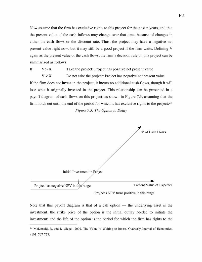
105
Now assume that the firm has exclusive rights to this project for the next n years, and that
the present value of the cash inflows may change over that time, because of changes in
either the cash flows or the discount rate. Thus, the project may have a negative net
present value right now, but it may still be a good project if the firm waits. Defining V
again as the present value of the cash flows, the firm’s decision rule on this project can be
summarized as follows:
If V > X Take the project: Project has positive net present value
V < X Do not take the project: Project has negative net present value
If the firm does not invest in the project, it incurs no additional cash flows, though it will
lose what it originally invested in the project. This relationship can be presented in a
payoff diagram of cash flows on this project, as shown in Figure 7.3, assuming that the
firm holds out until the end of the period for which it has exclusive rights to the project:23
Figure 7.3: The Option to Delay
Present Value of Expected Cash Flows
PV of Cash Flows
Initial Investment in Project
Project has negative NPV in this range
Project's NPV turns positive in this range
Note that this payoff diagram is that of a call option –– the underlying asset is the
investment, the strike price of the option is the initial outlay needed to initiate the
investment; and the life of the option is the period for which the firm has rights to the 23 McDonald, R. and D. Siegel, 2002, The Value of Waiting to Invest, Quarterly Journal of Economics,
v101, 707-728.

106
investment. The present value of the cash flows on this project and the expected variance
in this present value represent the value and variance of the underlying asset.
Valuing an Option to Delay
On the surface, the inputs needed to apply option pricing theory to valuing the
option to delay are the same as those needed for any option. We need the value of the
underlying asset, the variance in that value, the time to expiration on the option, the strike
price, the riskless rate and the equivalent of the dividend yield (cost of delay). Actually
estimating these inputs for product patent valuation can be difficult, however.
a. Value Of The Underlying Asset: In this case, the underlying asset is the investment
itself. The current value of this asset is the present value of expected cash flows from
initiating the project now, not including the up-front investment, which can be obtained
by doing a standard capital budgeting analysis.
b. Variance in the value of the asset: The present value of the expected cashflows that
measures the value of the asset will change over time, partly because the potential market
size for the product may be unknown, and partly because technological shifts can change
the cost structure and profitability of the product. The variance in the present value of
cash flows from the project can be estimated in one of three ways.
• If similar projects have been introduced in the past, the variance in the cash flows
from those projects can be used as an estimate. This may be the way that a consumer
product company like Gillette might estimate the variance associated with introducing
a new blade for its razors.
• Probabilities can be assigned to various market scenarios, cash flows estimated under
each scenario and the variance estimated across present values. Alternatively, the
probability distributions can be estimated for each of the inputs into the project
analysis - the size of the market, the market share and the profit margin, for instance -
and simulations used to estimate the variance in the present values that emerge.
• The variance in the market value of publicly traded firms involved in the same
business (as the project being considered) can be used as an estimate of the variance.
Thus, the average variance in firm value of firms involved in the software business
can be used as the variance in present value of a software project.

107
The value of the option is largely derived from the variance in cash flows - the higher the
variance, the higher the value of the project delay option. Thus, the value of an option to
delay a project in a stable business will be less than the value of a similar option in an
environment where technology, competition and markets are all changing rapidly.
c. Exercise Price On Option: A project delay option is exercised when the firm owning
the rights to the project decides to invest in it. The cost of making this investment is the
exercise price of the option. The underlying assumption is that this cost remains constant
(in present value dollars) and that any uncertainty associated with the product is reflected
in the present value of cash flows on the product.
d. Expiration Of The Option And The Riskless Rate The project delay option expires
when the rights to the project lapse; investments made after the project rights expire are
assumed to deliver a net present value of zero as competition drives returns down to the
required rate. The riskless rate to use in pricing the option should be the rate that
corresponds to the expiration of the option. While this input can be estimated easily when
firms have the explicit right to a project (through a license or a patent, for instance), it
becomes far more difficult to obtain when firms only have a competitive advantage to
take a project.
d. Cost of Delay (Dividend Yield): There is a cost to delaying taking a project, once the
net present value turns positive. Since the project rights expire after a fixed period, and
excess profits (which are the source of positive present value) are assumed to disappear
after that time as new competitors emerge, each year of delay translates into one less year
of value-creating cash flows.24 If the cash flows are evenly distributed over time, and the
life of the patent is n years, the cost of delay can be written as:
€
Annual cost of delay = 1n
Thus, if the project rights are for 20 years, the annual cost of delay works out to 5% a
year. Note, though, that this cost of delay rises each year , to 1/19 in year 2, 1/18 in year 3
and so on, making the cost of delaying exercise larger over time.
24 A value-creating cashflow is one that adds to the net present value because it is in excess of the required
return for investments of equivalent risk.

108
Practical Considerations
While it is quite clear that the option to delay is embedded in many investments,
there are several problems associated with the use of option pricing models to value these
options. First, the underlying asset in this option, which is the project, is not traded,
making it difficult to estimate its value and variance. We would argue that the value can
be estimated from the expected cash flows and the discount rate for the project, albeit
with error. The variance is more difficult to estimate, however, since we are attempting
the estimate a variance in project value over time.
Second, the behavior of prices over time may not conform to the price path
assumed by the option pricing models. In particular, the assumption that prices move in
small increments continuously (an assumption of the Black-Scholes model), and that the
variance in value remains unchanged over time, may be difficult to justify in the context
of a real investment. For instance, a sudden technological change may dramatically
change the value of a project, either positively or negatively.
Third, there may be no specific period for which the firm has rights to the project.
For instance, a firm may have significant advantages over its competitors, which may, in
turn, provide it with the virtually exclusive rights to a project for a period of time. The
rights are not legal restrictions, however, and could erode faster than expected. In such
cases, the expected life of the project itself is uncertain and only an estimate. Ironically,
uncertainty about the expected life of the option can increase the variance in present
value, and through it, the expected value of the rights to the project.
Applications of Option to Delay
The option to delay provides interesting perspectives on three common
investment problems. The first is in the valuation of patents, especially those that are not
viable today but could be viable in the future; by extension, this will also allow us to look
at whether R&D expenses are delivering value. The second is in the analysis of natural
resource assets – vacant land, undeveloped oil reserves etc.
Patents
A product patent provides a firm with the right to develop and market a product.
The firm will do so only if the present value of the expected cash flows from the product
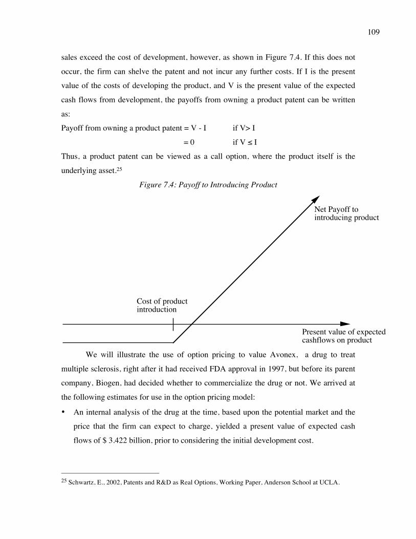
109
sales exceed the cost of development, however, as shown in Figure 7.4. If this does not
occur, the firm can shelve the patent and not incur any further costs. If I is the present
value of the costs of developing the product, and V is the present value of the expected
cash flows from development, the payoffs from owning a product patent can be written
as:
Payoff from owning a product patent = V - I if V> I
= 0 if V ≤ I
Thus, a product patent can be viewed as a call option, where the product itself is the
underlying asset.25
Figure 7.4: Payoff to Introducing Product
We will illustrate the use of option pricing to value Avonex, a drug to treat
multiple sclerosis, right after it had received FDA approval in 1997, but before its parent
company, Biogen, had decided whether to commercialize the drug or not. We arrived at
the following estimates for use in the option pricing model:
• An internal analysis of the drug at the time, based upon the potential market and the
price that the firm can expect to charge, yielded a present value of expected cash
flows of $ 3.422 billion, prior to considering the initial development cost.
25 Schwartz, E., 2002, Patents and R&D as Real Options, Working Paper, Anderson School at UCLA.
Present value of expectedcashflows on product
Net Payoff to introducing product
Cost of productintroduction

110
• The initial cost of developing the drug for commercial use was estimated to be $2.875
billion, if the drug was introduced immediately.
• The firm had the patent on the drug for the next 17 years, and the 17-year Treasury
bond rate was 6.7%.
• The average historical variance in market value for publicly traded bio-technology
firms was 0.224.
• It was assumed that the potential for excess returns exists only during the patent life,
and that competition will wipe out excess returns beyond that period. Thus, any delay
in introducing the drug, once it is viable, will cost the firm one year of patent-
protected excess returns. (For the initial analysis, the cost of delay will be 1/17, the
following year, it will be 1/16, the year after, 1/15 and so on.)
Based on these assumptions, we obtained the following inputs to the option pricing
model.
Present Value of Cash Flows from Introducing Drug Now = S = $ 3.422 billion
Initial Cost of Developing Drug for commercial use = K = $ 2.875 billion
Patent life = t = 17 years Riskless Rate = r = 6.7% (17-year T.Bond rate)
Variance in Expected Present Values =σ2 = 0.224
Expected Cost of Delay = y = 1/17 = 5.89%
Using these inputs in an option pricing model, we derived a value of $907 million for the
option,26 and this can be considered to be the real options value attached to the patent on
Avonex. To provide a contrast, the net present value of this patent is only $ 547 million:
NPV = $3,422 million - $ 2,875 million = $ 547 million
The time premium of $ 360 million ($907 million -$547 million) on this option suggests
that the firm will be better off waiting rather than developing the drug immediately, the
cost of delay notwithstanding. However, the cost of delay will increase over time, and
make exercise (development) more likely. Note also that we are assuming that the firm is
protected from all competition for the life of the patent. In reality, there are other
pharmaceutical firms working on their own drugs to treat multiple sclerosis and that can
26 This value was derived from using a Black Scholes model with these inputs. With a binomial model, the
estimated value increases slightly to $915 million.
111
affect both the option value and the firm’s behavior. In particular, if we assume that
Upjohn or Pfizer has a competing drug working through the FDA pipeline and that the
drug is expected to reach the market in 6 years, the cost of delay will increase to 16.67%
(1/6) and the option value will dissipate.
The implications of viewing patents as options can be significant. First, it implies
that non-viable patents will continue to have value, especially in businesses where there
is substantial volatility. Second, it indicates that firms may hold off on developing viable
patents, if they feel that they gain more from waiting than they lose in terms of cash
flows; this behavior will be more common if there is no significant competition on the
horizon. Third, the value of patents will be higher in risky businesses than in safe
businesses, since option value increases with volatility. If we consider R&D to be the
expense associated with acquiring these patents, this would imply that research should
have its biggest payoff when directed to areas where less is known and there is more
uncertainty. Consequently, we should expect pharmaceutical firms to spend more of their
R&D budgets on gene therapy than on flu vaccines.27
Natural Resource Options
In a natural resource investment, the underlying asset is the natural resource and
the value of the asset is based upon two variables - (1) the estimated quantity, and (2) the
price of the resource. Thus, in a gold mine, for example, the value of the underlying asset
is the value of the estimated gold reserves in the mine, based upon the current price of
gold. In most such investments, there is an initial cost associated with developing the
resource; the difference between the value of the asset extracted and the cost of the
development is the profit to the owner of the resource (see Figure 7.5). Defining the cost
of development as X, and the estimated value of the developed resource as V, the
potential payoffs on a natural resource option can be written as follows:
27 Pakes, A., 1986, Patents as Options: Some Estimates of the Value of Holding European Patent Stocks,
Econometrica, v54, 755-784. While this paper does not explicitly value patents as options, it examines the
returns investors would have earned investing in companies that derive their value from patents. The return
distribution resembles that of a portfolio of options, with most investments losing money but the winners
providing disproportionate gains.

112
Payoff on natural resource investment = V - X if V > X
= 0 if V≤ X
Thus, the investment in a natural resource option has a payoff function similar to a call
option.28
Figure 7.5: Payoff from Developing Natural Resource Reserves
To value a natural resource investment as an option, we need to make assumptions about
a number of variables:
1. Available reserves of the resource: Since this is not known with certainty at the outset,
it has to be estimated. In an oil tract, for instance, geologists can provide reasonably
accurate estimates of the quantity of oil available in the tract.
2. Estimated cost of developing the resource: The estimated development cost is the
exercise price of the option. Again, a combination of knowledge about past costs and the
specifics of the investment have to be used to come up with a reasonable measure of
development cost.
3. Time to expiration of the option: The life of a natural resource option can be defined in
one of two ways. First, if the ownership of the investment has to be relinquished at the
end of a fixed period of time, that period will be the life of the option. In many offshore
28 Brennan, M. and E. Schwartz, 1985, Evaluating Natural Resource Investments, The Journal of Business,
v58, 135-157.
Value of estimated reserveof natural resource
Net Payoff on extracting reserve
Cost of Developing reserve

113
oil leases, for instance, the oil tracts are leased to the oil company for several years. The
second approach is based upon the inventory of the resource and the capacity output rate,
as well as estimates of the number of years it would take to exhaust the inventory. Thus, a
gold mine with a mine inventory of 3 million ounces and a capacity output rate of
150,000 ounces a year will be exhausted in 20 years, which is defined as the life of the
natural resource option.
4. Variance in value of the underlying asset: The variance in the value of the underlying
asset is determined by two factors – (1) variability in the price of the resource, and (2)
variability in the estimate of available reserves. In the special case where the quantity of
the reserve is known with certainty, the variance in the underlying asset's value will
depend entirely upon the variance in the price of the natural resource. In the more
realistic case where the quantity of the reserve and the oil price can change over time, the
option becomes more difficult to value; here, the firm may have to invest in stages to
exploit the reserves.
5. Cost of Delay: The net production revenue as a percentage of the market value of the
reserve is the equivalent of the dividend yield and is treated the same way in calculating
option values. An alternative way of thinking about this cost is in terms of a cost of delay.
Once a natural resource option is in-the-money (Value of the reserves > Cost of
developing these reserves), the firm, by not exercising the option, is costing itself the
production revenue it could have generated by developing the reserve.
An important issue in using option pricing models to value natural resource
options is the effect of development lags on the value of these options. Since the
resources cannot be extracted instantaneously, a time lag has to be allowed between the
decision to extract the resources and the actual extraction. A simple adjustment for this
lag is to reduce the value of the developed reserve to reflect the loss of cash flows during
the development period. Thus, if there is a one-year lag in development, the current value
of the developed reserve will be discounted back one year at the net production
revenue/asset value ratio29 (which we also called the dividend yield above).30
29 Intuitively, it may seem like the discounting should occur at the riskfree rate. The simplest way of
explaining why we discount at the dividend yield is to consider the analogy with a listed option on a stock.

114
To illustrate the use of option pricing to value natural reserves, consider an
offshore oil property with an estimated reserve of 50 million barrels of oil; the cost of
developing the reserve is expected to be $ 600 million, and the development lag is two
years. The firm has the rights to exploit this reserve for the next 20 years, and the
marginal value per barrel of oil is $12 currently31 (price per barrel - marginal cost per
barrel). Once developed, the net production revenue each year will be 5% of the value of
the reserves. The riskless rate is 8%, and the variance in ln(oil prices) is 0.03. Given this
information, the inputs to the option pricing model can be estimated as follows:
Current Value of the asset = S = Value of the developed reserve discounted back
the length of the development lag at the dividend yield = $12 * 50 /(1.05)2 = $
544.22
If development is started today, the oil will not be available for sale until two years from
now. The estimated opportunity cost of this delay is the lost production revenue over the
delay period; hence, the discounting of the reserve back at the dividend yield.
Exercise Price = Cost of developing reserve = $ 600 million (assumed to be both
known and fixed over time)
Time to expiration on the option = 20 years
In this example, we assume that the only uncertainty is in the price of oil, and the
variance therefore becomes the variance in oil prices.
Variance in the value of the underlying asset (oil) = 0.03
Riskless rate =8%
Dividend Yield = Net production revenue / Value of reserve = 5%
Assume that on exercising a listed option on a stock, you had to wait six months for the stock to be
delivered to you. What you lose is the dividends you would have received over the six-month period by
holding the stock. Hence, the discounting is at the dividend yield.
30 Brennan, M.J., and E.S. Schwartz, 1985, Evaluating Natural Resource Investments, Journal of Business 58, pp. 135-157. 31 For simplicity, we will assume that while this marginal value per barrel of oil will grow over time, the
present value of the marginal value will remain unchanged at $ 12 per barrel. If we do not make this
assumption, we will have to estimate the present value of the oil that will be extracted over the extraction
period.

115
Based upon these inputs, the option pricing model yields an estimate of value of $97.08
million.32 This oil reserve, though not viable at current prices, is still a valuable property
because of its potential to create value if oil prices go up.33
The same type of analysis can be extended to any other commodity company
(gold and copper reserves, for instance) and even to vacant land or real estate properties.
The owner of vacant land in Manhattan can choose whether and when to develop the land
and will make that decision based upon real estate values. 34
What are the implications of viewing natural resource reserves as options? The
first is that the value of a natural resource company can be written as a sum of two
values: the conventional risk adjusted value of expected cash flows from developed
reserves and the option value of undeveloped reserves. While both will increase in value
as the price of the natural resource increases, the latter will respond positively to
increases in price volatility. Thus, the values of oil companies should increase if oil price
volatility increases, even if oil prices themselves do not go up. The second is that
conventional discounted cash flow valuation will understate the value of natural resource
companies, even if the expected cash flows are unbiased and reasonable because it will
miss the option premium inherent in their undeveloped reserves. The third is that
development of natural resource reserves will slow down as the volatility in prices
increases; the time premium on the options will increase, making exercise of the options
(development of the reserves) less likely.
Mining and commodity companies have been at the forefront in using real options
in decision making and their usage of the technology predates the current boom in real
options. One reason is that natural resource options come closest to meeting the pre-
requisites for the use of option pricing models. Firms can learn a great deal by observing 32 This is the estimate from a Black-Scholes model, with a dividend yield adjustment. Using a binomial
model yields an estimate of value of $ 101 million. 33 Paddock, J.L. & D. R. Siegel & J.L. Smith (1988): “Option Valuation of Claims on Real Assets: The Case of Offshore Petroleum Leases”, Quarterly Journal of Economics, August 1988, pp.479-508. This paper provides a detailed examination of the application of real options to value oil reserves. They applied the model to examine the prices paid for offshore oil leases in the US in 1980 and concluded that companies over paid (relative to the option value). 34 Quigg, L, 1993] Empirical Testing of Real Option-Pricing Models », Journal of Finance, vol.48, 621-640. The author examined transaction data on 2700 undeveloped and 3200 developed real estate properties between 1976-79 and found evidence of a premium arising from the option to wait in the former.

116
commodity prices and can adjust their behavior (in terms of development and
exploration) quickly. In addition, if we consider exclusivity to be a pre-requisite for real
options to have value, that exclusivity for natural resource options derives from their
natural scarcity; there is, after all, only a finite amount of oil and gold under the ground
and vacant land in Manhattan. Finally, natural resource reserves come closest to meeting
the arbitrage/replication requirements that option pricing models are built upon; both the
underlying asset (the natural resource) and the option can often be bought and sold.
The Option to Expand
In some cases, a firm will take an investment because doing so allows it either to
make other investments or to enter other markets in the future. In such cases, it can be
argued that the initial investment provides the firm with an option to expand, and the firm
should therefore be willing to pay a price for such an option. Consequently, a firm may
be willing to lose money on the first investment because it perceives the option to expand
as having a large enough value to compensate for the initial loss.
To examine this option, assume that the present value of the expected cash flows
from entering the new market or taking the new project is V, and the total investment
needed to enter this market or take this project is X. Further, assume that the firm has a
fixed time horizon, at the end of which it has to make the final decision on whether or not
to take advantage of this opportunity. Finally, assume that the firm cannot move forward
on this opportunity if it does not take the initial investment. This scenario implies the
option payoffs shown in Figure 7.6.

117
Figure 7.6: The Option to Expand
Present Value of Expected Cash Flows
PV of Cash Flows
Cost of Expansion
Expansion has negative NPV in this range Expansion NPV turns positive in this range
As you can see, at the expiration of the fixed time horizon, the firm will enter the new
market or take the new investment if the present value of the expected cash flows at that
point in time exceeds the cost of entering the market.
Consider a simple example of an option to expand. Disney is considering starting
a Spanish version of the Disney Channel in Mexico and estimates the net present value of
this investment to be -$150 million. While the negative net present value would normally
suggest that rejecting the investment is the best course, assume that if the Mexican
venture does better than expected, Disney plans to expand the network to the rest of
South America at a cost of $ 500 million. Based on its current assessment of this market,
Disney believes that the present value of the expected cash flows on this investment is
only $ 400 million (making it a negative net present value investment as well). The
saving grace is that the latter present value is an estimate and Disney does not have a firm
grasp of the market; a Monte Carlo simulation of the investments yields a standard
deviation of 50% in value. Finally, assume that Disney will have to make this expansion
decision within 5 years of the Mexican investment, and that the five-year riskfree rate is
4%. The value of the expansion option can now be computed using the inputs:
S = Present value of expansion cash flows = $ 400 million
118
K = Cost of expansion = $ 500 million
σ = Standard deviation in value (from simulation) = 50%
t = 5 years
r = 4%
The resulting option value is $167 million.35
The practical considerations associated with estimating the value of the option to
expand are similar to those associated with valuing the option to delay. In most cases,
firms with options to expand have no specific time horizon by which they have to make
an expansion decision, making these open-ended options, or, at best, options with
arbitrary lives. Even in those cases where a life can be estimated for the option, neither
the size nor the potential market for the product may be known, and estimating either can
be problematic. To illustrate, consider the Disney example discussed above. While we
adopted a period of five years, at the end of which the Disney has to decide one way or
another on its future expansion into South America, it is entirely possible that this time
frame is not specified at the time the store is opened. Furthermore, we have assumed that
both the cost and the present value of expansion are known initially. In reality, the firm
may not have good estimates for either before making the first investment, since it does
not have much information on the underlying market.
Implications
The option to expand is implicitly used by firms to rationalize taking investments
that have negative net present value, but provide significant opportunities to tap into new
markets or sell new products. While the option pricing approach adds rigor to this
argument by estimating the value of this option, it also provides insight into those
occasions when it is most valuable. In general, the option to expand is clearly more
valuable for more volatile businesses with higher returns on projects (such as
biotechnology or computer software), than in stable businesses with lower returns (such
as housing, utilities or automobile production). Specifically, the option to expand is at the
basis of arguments that an investment should be made because of strategic considerations
or that large investments should be broken up into smaller phases. It can also be 35 This value was computed using the Black-Scholes model. A binomial model yields a similar value.

119
considered a rationale for why firms may accumulate cash or hold back on borrowing,
thus preserving financial flexibility.
Strategic Considerations
In many acquisitions or investments, the acquiring firm believes that the
transaction will give it competitive advantages in the future. These competitive
advantages range the gamut, and include:
• Entrée into a Growing or Large Market: An investment or acquisition may allow the
firm to enter a large or potentially large market much sooner than it otherwise would
have been able to do so. A good example of this would be the acquisition of a
Mexican retail firm by a US firm, with the intent of expanding into the Mexican
market.
• Technological Expertise: In some cases, the acquisition is motivated by the desire to
acquire a proprietary technology, that will allow the acquirer to expand either its
existing market or into a new market.
• Brand Name: Firms sometime pay large premiums over market price to acquire firms
with valuable brand names, because they believe that these brand names can be used
for expansion into new markets in the future.
While all of these potential advantages may be used to justify initial investments that do
not meet financial benchmarks, not all of them create valuable options. The value of the
option is derived from the degree to which these competitive advantages, assuming that
they do exist, translate into sustainable excess returns. As a consequence, these
advantages can be used to justify premiums only in cases where the acquiring firm
believes that it has some degree of exclusivity in the targeted market or technology. Two
examples can help illustrate this point. A telecommunications firm should be willing to
pay a premium for Chinese telecomm firm, if the latter has exclusive rights to service a
large segment of the Chinese market; the option to expand in the Chinese market could
be worth a significant amount.36 On the other hand, a developed market retailer should be 36 A note of caution needs to be added here. If the exclusive rights to a market come with no pricing power
– in other words, the Government will set the price you charge your customers – it may very well translate
into zero excess returns (and no option value).

120
wary about paying a real option premium for an Indian retail firm, even though it may
believe that the Indian market could grow to be a lucrative one. The option to expand into
this lucrative market is open to all entrants and not just to existing retailers and thus may
not translate into sustainable excess returns.
Multi-Stage Projects/ Investments
When entering new businesses or making new investments, firms sometimes have
the option to enter the business in stages. While doing so may reduce potential upside, it
also protects the firm against downside risk, by allowing it, at each stage, to gauge
demand and decide whether to go on to the next stage. In other words, a standard project
can be recast as a series of options to expand, with each option being dependent on the
previous one. There are two propositions that follow:
• Some projects that do not look good on a full investment basis may be value creating
if the firm can invest in stages.
• Some projects that look attractive on a full investment basis may become even more
attractive if taken in stages.
The gain in value from the options created by multi-stage investments has to be weighed
off against the cost. Taking investments in stages may allow competitors who decide to
enter the market on a full scale to capture the market. It may also lead to higher costs at
each stage, since the firm is not taking full advantage of economies of scale.
There are several implications that emerge from viewing this choice between
multi-stage and one-time investments in an option framework. The projects where the
gains will be largest from making the investment in multiple stages include:
(1) Projects where there are significant barriers to entry from competitors entering the
market, and taking advantage of delays in full-scale production. Thus, a firm with a
patent on a product or other legal protection against competition pays a much smaller
price for starting small and expanding as it learns more about the product
(2) Projects where there is significant uncertainty about the size of the market and the
eventual success of the project. Here, starting small and expanding allows the firm to
reduce its losses if the product does not sell as well as anticipated, and to learn more
about the market at each stage. This information can then be useful in subsequent
121
stages in both product design and marketing. Hsu argues that venture capitalists
invest in young companies in stages, partly to capture the value of option of
waiting/learning at each stage and partly to reduce the likelihood that the entrepreneur
will be too conservative in pursuing risky (but good) opportunities.37
(3) Projects where there is a substantial investment needed in infrastructure (large fixed
costs) and high operating leverage. Since the savings from doing a project in multiple
stages can be traced to investments needed at each stage, they are likely to be greater
in firms where those costs are large. Capital intensive projects as well as projects that
require large initial marketing expenses (a new brand name product for a consumer
product company) will gain more from the options created by taking the project in
multiple stages.
Growth Companies
In the stock market boom in the 1990s, we witnessed the phenomenon of young,
start-up, internet companies with large market capitalizations but little to show in terms
of earnings, cash flows or even revenues. Conventional valuation models suggested that it
would be difficult, if not impossible, to justify these market valuations with expected
cash flows. In an interesting twist on the option to expand argument, there were some
who argued that investors in these companies were buying options to expand and be part
of a potentially huge e-commerce market, rather than conventional stock.38
While the argument is alluring and serves to pacify investors in growth companies
who may feel that they are paying too much, there are clearly dangers in making this
stretch. The biggest one is that the “exclusivity” component that is necessary for real
options to have value is being given short shrift. Consider investing in an internet stock in
1999 and assume that you are paying a premium to be part of a potentially large online
market in 2008. Assume further that this market comes to fruition. Could you partake in
this market without paying that upfront premium a dot-com company? We don’t see why
37 Hsu, Y., 2002, Staging of Venture Capital Investment: A Real Options Analysis, Working paper,
University of Cambridge. 38 Schwartz, E.S. and M. Moon, 2001, Rational Pricing of Internet Companies Revisited, The Financial Review 36, pp. 7-26. A simpler version of the same argument was made in Mauboussin, M., 1998, Get Real: Using Real Options in Security Analysis, CSFB Publication, June 23, 1999.
122
not. After all, GE and Nokia are just as capable of being part of this online market, as are
any number of new entrants into the market.39
The Option to Abandon an Investment
The final option to consider here is the option to abandon a project when its cash
flows do not measure up to expectations. One way to reflect this value is through decision
trees. The decision tree has limited applicability in most real world investment analyses;
it typically works only for multi-stage projects, and it requires inputs on probabilities at
each stage of the project. The option pricing approach provides a more general way of
estimating and building in the value of abandonment into investment analysis. To
illustrate, assume that V is the remaining value on a project if it continues to the end of its
life, and L is the liquidation or abandonment value for the same project at the same point
in time. If the project has a life of n years, the value of continuing the project can be
compared to the liquidation (abandonment) value. If the value from continuing is higher,
the project should be continued; if the value of abandonment is higher, the holder of the
abandonment option could consider abandoning the project .
Payoff from owning an abandonment option = 0 if V > L
= L-V if V ≤ L
These payoffs are graphed in Figure 7.7, as a function of the expected value from
continuing the investment.
39 This argument is fleshed out in my book, “The Dark Side of Valuation”, published by Prentice-Hall.

123
Figure 7.7: The Option to Abandon
PV of Cash Flows from project
Salvage Value from Abandonment
Unlike the prior two cases, the option to abandon takes on the characteristics of a put
option.
Consider a simple example. Assume that a firm is considering taking a 10-year
project that requires an initial investment of $ 100 million in a real estate partnership,
where the present value of expected cash flows is $ 110 million. While the net present
value of $ 10 million is small, assume that the firm has the option to abandon this project
anytime in the next 10 years, by selling its share of the ownership to the other partners in
the venture for $ 50 million. Assume that the variance in the present value of the
expected cash flows from being in the partnership is 0.09.
The value of the abandonment option can be estimated by determining the
characteristics of the put option:
Value of the Underlying Asset (S) = PV of Cash Flows from Project
= $ 110 million
Strike Price (K) = Salvage Value from Abandonment = $ 50 million
Variance in Underlying Asset’s Value = 0.09
Time to expiration = Period for which the firm has abandonment option = 10 years
The project has a 25-year life and is expected to lose value each year; for simplicity, we
will assume that the loss is linear (4% a year).
Loss in value each year = 1/n = 1/25 = 4%

124
Assume that the ten-year riskless rate is 6%. The value of the put option can be estimated
as follows:
Call Value = 110 exp(-.04)(10) (0.9737) -50 (exp(-0.06)(10) (0.8387) = $ 84.09 million
Put Value= $ 84.09 - 110 + 50 exp(-0.06)(10) = $ 1.53 million
The value of this abandonment option has to be added on to the net present value of the
project of $ 10 million, yielding a total net present value with the abandonment option of
$ 11.53 million. Note though that abandonment becomes a more and more attractive
option as the remaining project life decreases, since the present value of the remaining
cash flows will decrease.
In the above analysis, we assumed, rather unrealistically, that the abandonment
value was clearly specified up front and that it did not change during the life of the
project. This may be true in some very specific cases, in which an abandonment option is
built into the contract. More often, however, the firm has the option to abandon, and the
salvage value from doing so has to be estimated (with error) up front. Further, the
abandonment value may change over the life of the project, making it difficult to apply
traditional option pricing techniques. Finally, it is entirely possible that abandoning a
project may not bring in a liquidation value, but may create costs instead; a
manufacturing firm may have to pay severance to its workers, for instance. In such cases,
it would not make sense to abandon, unless the present value of the expected cash flows
from continuing with the investment are even more negative.
Implications
The fact that the option to abandon has value provides a rationale for firms to
build in operating flexibility to scale back or terminate projects if they do not measure up
to expectations. It also indicates that firms that focus on generating more revenues by
offering their customers the option to walk away from commitments may be giving up
more than they gain, in the process.
1. Escape Clauses
When a firm enters into a long term risky investment that requires a large up front
investment, it should do so with the clear understanding that it may regret making this

125
investment fairly early in its life. Being able to get out of such long-term commitments
that threaten to drain more resources in the future is at the heart of the option to abandon.
It is true that some of this flexibility is determined by the business that you are in; getting
out of bad investments is easier to do in service businesses than in heavy infrastructure
businesses. However, it is also true that there are actions that firms can take at the time of
making these investments that give them more choices, if things do not go according to
plan.
The first and most direct way is to build operating flexibility contractually with
those parties that are involved in the investment. Thus, contracts with suppliers may be
written on an annual basis, rather than long term, and employees may be hired on a
temporary basis, rather than permanently. The physical plant used for a project may be
leased on a short-term basis, rather than bought, and the financial investment may be
made in stages rather than as an initial lump sum. While there is a cost to building in this
flexibility, the gains may be much larger, especially in volatile businesses. The initial
capital investment can be shared with another investor, presumably with deeper pockets
and a greater willingness to stay with the investment, even if it turns sour. This provides a
rationale for join venture investing, especially for small firms that have limited resources;
finding a cash-rich, larger company to share the risk may well be worth the cost.
None of these actions are costless. Entering into short term agreements with
suppliers and leasing the physical plant may be more expensive than committing for the
life of the investment, but that additional cost has to be weighed off against the benefit of
maintaining the abandonment option.
2. Customer Incentives
Firms that are intent on increasing revenues sometimes offer abandonment
options to customers to induce them to buy their products and services. As an example,
consider a firm that sells its products on multi-year contracts and offers customers the
option to cancel their contracts at any time, with no cost. While this may sweeten the deal
and increase sales, there is likely to be a substantial cost. In the event of a recession,
customers that are unable to meet their obligations are likely to cancel their contracts. In
effect, the firm has made its good times better and its bad times worse; the cost of this

126
increased volatility in earnings and revenues has to be measured against the potential gain
in revenue growth to see if the net effect is positive.
This discussion should also act as a cautionary note for those firms that are run
with marketing objectives such as maximizing market share or posting high revenue
growth. Those objectives can often be accomplished by giving valuable options to
customers – sales people will want to meet their sales targets and are not particularly
concerned about the long term costs they may create with their commitments to
customers – and the firm may be worse off as a consequence.
3. Switching Options
While the abandonment option considers the value of shutting an investment
down entirely, there is an intermediate alternative that is worth examining. Firms can
sometimes alter production levels in response to demand and being able to do so can
make an investment more valuable. Consider, for instance, a power company that is
considering a new plant to generate electricity and assume that the company can run the
plant at full capacity and produce 1 million kilowatt hours of power or at half capacity
(and substantially less cost) and produce 500,000 kilowatt hours of power. In this case,
the company can observe both the demand for power and the revenues per kilowatt-hour
and decide whether it makes sense to run at full or half capacity. The value of this
switching option can then be compared to the cost of building in this flexibility in the first
place.
The airline business provides an interesting case study in how different companies
manage their cost structure and the payoffs to their strategies. One reason that Southwest
Airlines has been able to maintain its profitability in a deeply troubled sector is that the
company has made cost flexibility a central component in its decision process. From its
choice of using only one type of aircraft for its entire fleet40 to its refusal, for the most
part, to fly into large urban airports (with high gate costs), the company’s operations have
created the most flexible cost structure in the business. Thus, when revenues dip (as they
40 From its inception until recently, Southwest used the Boeing 737 as its workhorse, thus reducing its need
to maintain different maintenance crews at each airport it flies into.

127
inevitably do at some point in time when the economy weakens), Southwest is able to
trim its costs and stay profitable while other airlines teeter on the brink of bankruptcy.
Caveats on Real Options The discussion on the potential applications of real options should provide a
window into why they are so alluring to practitioners and businesses. In essence, we are
ignoring that the time honored rules of capital budgeting, which include rejecting
investments that have negative net present value, when real options are present. Not only
does the real options approach encourage you to make investments that do not meet
conventional financial criteria, it also makes it more likely that you will do so, the less
you know about the investment. Ignorance, rather than being a weakness, becomes a
virtue because it pushes up the uncertainty in the estimated value and the resulting option
value. To prevent the real options process from being hijacked by managers who want to
rationalize bad (and risky) decisions, we have to impose some reasonable constraints on
when it can be used and when it is used, how to estimate its value.
First, not all investments have options embedded in them, and not all options, even if
they do exist, have value. To assess whether an investment creates valuable options that
need to be analyzed and valued, three key questions need to be answered affirmatively.
• Is the first investment a pre-requisite for the later investment/expansion? If not, how
necessary is the first investment for the later investment/expansion? Consider our
earlier analysis of the value of a patent or the value of an undeveloped oil reserve as
options. A firm cannot generate patents without investing in research or paying
another firm for the patents, and it cannot get rights to an undeveloped oil reserve
without bidding on it at a government auction or buying it from another oil company.
Clearly, the initial investment here (spending on R&D, bidding at the auction) is
required for the firm to have the second option. Now consider the Disney expansion
into Mexico. The initial investment in a Spanish channel provides Disney with
information about market potential, without which presumably it is unwilling to
expand into the larger South American market. Unlike the patent and undeveloped
reserves illustrations, the initial investment is not a pre-requisite for the second,
though management might view it as such. The connection gets even weaker when

128
we look at one firm acquiring another to have the option to be able to enter a large
market. Acquiring an internet service provider to have a foothold in the internet
retailing market or buying a Brazilian brewery to preserve the option to enter the
Brazilian beer market would be examples of such transactions.
• Does the firm have an exclusive right to the later investment/expansion? If not, does
the initial investment provide the firm with significant competitive advantages on
subsequent investments? The value of the option ultimately derives not from the cash
flows generated by then second and subsequent investments, but from the excess
returns generated by these cash flows. The greater the potential for excess returns on
the second investment, the greater the value of the option in the first investment. The
potential for excess returns is closely tied to how much of a competitive advantage
the first investment provides the firm when it takes subsequent investments. At one
extreme, again, consider investing in research and development to acquire a patent.
The patent gives the firm that owns it the exclusive rights to produce that product, and
if the market potential is large, the right to the excess returns from the project. At the
other extreme, the firm might get no competitive advantages on subsequent
investments, in which case, it is questionable as to whether there can be any excess
returns on these investments. In reality, most investments will fall in the continuum
between these two extremes, with greater competitive advantages being associated
with higher excess returns and larger option values.
• How sustainable are the competitive advantages? In a competitive market place,
excess returns attract competitors, and competition drives out excess returns. The
more sustainable the competitive advantages possessed by a firm, the greater will be
the value of the options embedded in the initial investment. The sustainability of
competitive advantages is a function of two forces. The first is the nature of the
competition; other things remaining equal, competitive advantages fade much more
quickly in sectors where there are aggressive competitors and new entry into the
business is easy. The second is the nature of the competitive advantage. If the
resource controlled by the firm is finite and scarce (as is the case with natural
resource reserves and vacant land), the competitive advantage is likely to be
sustainable for longer periods. Alternatively, if the competitive advantage comes from

129
being the first mover in a market or technological expertise, it will come under assault
far sooner. The most direct way of reflecting this in the value of the option is in its
life; the life of the option can be set to the period of competitive advantage and only
the excess returns earned over this period counts towards the value of the option.
Second, when real options are used to justify a decision, the justification has to be in
more than qualitative terms. In other words, managers who argue for taking a project with
poor returns or paying a premium on an acquisition on the basis of real options, should be
required to value these real options and show, in fact, that the economic benefits exceed
the costs. There will be two arguments made against this requirement. The first is that
real options cannot be easily valued, since the inputs are difficult to obtain and often
noisy. The second is that the inputs to option pricing models can be easily manipulated to
back up whatever the conclusion might be. While both arguments have some basis, an
estimate with error is better than no estimate at all, and the process of quantitatively
trying to estimate the value of a real option is, in fact, the first step to understanding what
drives it value.
There is one final note of caution that we should add about the use of option
pricing models to assess the value of real options. Option pricing models, be they of the
binomial or Black Scholes variety, are based on two fundamental precepts – replication
and arbitrage. For either to be feasible, you have to be able to trade on the underlying
asset and on the option. This is easy to accomplish with a listed option on a traded stock;
you can trade on both the stock and the listed option. It is much more difficult to pull off
when valuing a patent or an investment expansion opportunity; neither the underlying
asset (the product that emerges from the patent) nor the option itself are traded. This does
not mean that you cannot estimate the value of a patent as an option but it does indicate
that monetizing this value will be much more difficult to do. In the Avonex example from
earlier in the chapter, the option value for the patent was $907 million whereas the
conventional risk adjusted value was only $547 million. Much as you may believe in the
former as the right estimate of value, it is unlikely that any potential buyer of the patent
will come close to paying that amount.

130
Conclusion In this chapter, we considered three potential real options and applications of
each. The first is the option to delay, where a firm with exclusive rights to an investment
has the option of deciding when to take that investment and to delay taking it, if
necessary. The second is the option to expand, where a firm may be willing to lose
money on an initial investment, in the hope of expanding into other investments or
markets further down the road. The third is the option to abandon an investment, if it
looks like a money loser, early in the process.
While it is clearly appropriate to attach value to real options in some cases –
patents, reserves of natural resources or exclusive licenses – the argument for an option
premium gets progressively weaker as we move away from the exclusivity inherent in
each of these cases. In particular, a firm that invests into an emerging market in a money-
losing enterprise, using the argument that that market is a large and potentially profitable
one, could be making a serious mistake. After all, the firm could be right in its
assessment of the market, but absent barriers to entry, it may not be able to earn excess
returns in that market or keep the competition out. Not all opportunities are options and
not all options have significant economic value.

131
Appendix: Basics of Options and Option Pricing An option provides the holder with the right to buy or sell a specified quantity of
an underlying asset at a fixed price (called a strike price or an exercise price) at or before
the expiration date of the option. Since it is a right and not an obligation, the holder can
choose not to exercise the right and allow the option to expire. There are two types of
options - call options and put options.
Option Payoffs A call option gives the buyer of the option the right to buy the underlying asset at a
fixed price, called the strike or the exercise price, at any time prior to the expiration date
of the option: the buyer pays a price for this right. If at expiration, the value of the asset is
less than the strike price, the option is not exercised and expires worthless. If, on the
other hand, the value of the asset is greater than the strike price, the option is exercised -
the buyer of the option buys the stock at the exercise price and the difference between the
asset value and the exercise price comprises the gross profit on the investment. The net
profit on the investment is the difference between the gross profit and the price paid for
the call initially. A payoff diagram illustrates the cash payoff on an option at expiration.
For a call, the net payoff is negative (and equal to the price paid for the call) if the value
of the underlying asset is less than the strike price. If the price of the underlying asset
exceeds the strike price, the gross payoff is the difference between the value of the
underlying asset and the strike price, and the net payoff is the difference between the
gross payoff and the price of the call. This is illustrated in the figure 7A.1:

132
Figure 7A.1: Call Option – Payoff Diagram
Strike Price
Net Payoff
Price of Underlying Asset
A put option gives the buyer of the option the right to sell the underlying asset at a
fixed price, again called the strike or exercise price, at any time prior to the expiration
date of the option. The buyer pays a price for this right. If the price of the underlying
asset is greater than the strike price, the option will not be exercised and will expire
worthless. If on the other hand, the price of the underlying asset is less than the strike
price, the owner of the put option will exercise the option and sell the stock a the strike
price, claiming the difference between the strike price and the market value of the asset as
the gross profit. Again, netting out the initial cost paid for the put yields the net profit
from the transaction. A put has a negative net payoff if the value of the underlying asset
exceeds the strike price, and has a gross payoff equal to the difference between the strike
price and the value of the underlying asset if the asset value is less than the strike price.
This is summarized in figure 7A.2.

133
Figure 7A.2: Put Option – Payoff Diagram
Price of Underlying Asset
Strike Price
Net Payoff
There is one final distinction that needs to be made. Options are usually categorized as
American or European options. A primary distinction between two is that American
options can be exercised at any time prior to its expiration, while European options can
be exercised only at expiration. The possibility of early exercise makes American options
more valuable than otherwise similar European options; it also makes them more difficult
to value. There is one compensating factor that enables the former to be valued using
models designed for the latter. In most cases, the time premium associated with the
remaining life of an option and transactions costs makes early exercise sub-optimal. In
other words, the holders of in-the-money options will generally get much more by selling
the option to someone else than by exercising the options.41
41 While early exercise is not optimal generally, there are at least two exceptions to this rule. One is a case
where the underlying asset pays large dividends, thus reducing the value of the asset, and any call options
on that asset. In this case, call options may be exercised just before an ex-dividend date, if the time
premium on the options is less than the expected decline in asset value as a consequence of the dividend
payment. The other exception arises when an investor holds both the underlying asset and deep in-the-
money puts on that asset at a time when interest rates are high. In this case, the time premium on the put
may be less than the potential gain from exercising the put early and earning interest on the exercise price.

134
Determinants of Option Value The value of an option is determined by a number of variables relating to the
underlying asset and financial markets.
1. Current Value of the Underlying Asset : Options are assets that derive value from an
underlying asset. Consequently, changes in the value of the underlying asset affect the
value of the options on that asset. Since calls provide the right to buy the underlying asset
at a fixed price, an increase in the value of the asset will increase the value of the calls.
Puts, on the other hand, become less valuable as the value of the asset increase.
2. Variance in Value of the Underlying Asset: The buyer of an option acquires the right
to buy or sell the underlying asset at a fixed price. The higher the variance in the value of
the underlying asset, the greater the value of the option. This is true for both calls and
puts. While it may seem counter-intuitive that an increase in a risk measure (variance)
should increase value, options are different from other securities since buyers of options
can never lose more than the price they pay for them; in fact, they have the potential to
earn significant returns from large price movements.
3. Dividends Paid on the Underlying Asset: The value of the underlying asset can be
expected to decrease if dividend payments are made on the asset during the life of the
option. Consequently, the value of a call on the asset is a decreasing function of the size
of expected dividend payments, and the value of a put is an increasing function of
expected dividend payments. A more intuitive way of thinking about dividend payments,
for call options, is as a cost of delaying exercise on in-the-money options. To see why,
consider a option on a traded stock. Once a call option is in the money, i.e, the holder of
the option will make a gross payoff by exercising the option, exercising the call option
will provide the holder with the stock, and entitle him or her to the dividends on the stock
in subsequent periods. Failing to exercise the option will mean that these dividends are
foregone.
4. Strike Price of Option: A key characteristic used to describe an option is the strike
price. In the case of calls, where the holder acquires the right to buy at a fixed price, the
value of the call will decline as the strike price increases. In the case of puts, where the
holder has the right to sell at a fixed price, the value will increase as the strike price
increases.
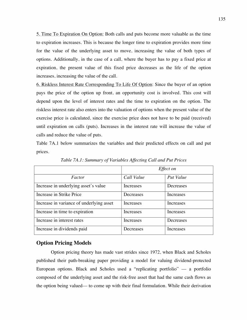
135
5. Time To Expiration On Option: Both calls and puts become more valuable as the time
to expiration increases. This is because the longer time to expiration provides more time
for the value of the underlying asset to move, increasing the value of both types of
options. Additionally, in the case of a call, where the buyer has to pay a fixed price at
expiration, the present value of this fixed price decreases as the life of the option
increases, increasing the value of the call.
6. Riskless Interest Rate Corresponding To Life Of Option: Since the buyer of an option
pays the price of the option up front, an opportunity cost is involved. This cost will
depend upon the level of interest rates and the time to expiration on the option. The
riskless interest rate also enters into the valuation of options when the present value of the
exercise price is calculated, since the exercise price does not have to be paid (received)
until expiration on calls (puts). Increases in the interest rate will increase the value of
calls and reduce the value of puts.
Table 7A.1 below summarizes the variables and their predicted effects on call and put
prices.
Table 7A.1: Summary of Variables Affecting Call and Put Prices
Effect on
Factor Call Value Put Value
Increase in underlying asset’s value Increases Decreases
Increase in Strike Price Decreases Increases
Increase in variance of underlying asset Increases Increases
Increase in time to expiration Increases Increases
Increase in interest rates Increases Decreases
Increase in dividends paid Decreases Increases
Option Pricing Models Option pricing theory has made vast strides since 1972, when Black and Scholes
published their path-breaking paper providing a model for valuing dividend-protected
European options. Black and Scholes used a “replicating portfolio” –– a portfolio
composed of the underlying asset and the risk-free asset that had the same cash flows as
the option being valued–– to come up with their final formulation. While their derivation

136
is mathematically complicated, there is a simpler binomial model for valuing options that
draws on the same logic.
The Binomial Model
The binomial option pricing model is based upon a simple formulation for the
asset price process, in which the asset, in any time period, can move to one of two
possible prices. The general formulation of a stock price process that follows the
binomial is shown in figure 7A.3.
Figure 7A.3: General Formulation for Binomial Price Path
In this figure, S is the current stock price; the price moves up to Su with probability p and
down to Sd with probability 1-p in any time period.
The objective in creating a replicating portfolio is to use a combination of risk-
free borrowing/lending and the underlying asset to create the same cash flows as the
option being valued. The principles of arbitrage apply here, and the value of the option
must be equal to the value of the replicating portfolio. In the case of the general
formulation above, where stock prices can either move up to Su or down to Sd in any
time period, the replicating portfolio for a call with strike price K will involve borrowing
$B and acquiring ∆ of the underlying asset, where:
∆ = Number of units of the underlying asset bought = (Cu - Cd)/(Su - Sd)
where,
S
Su
Sd
Su2
Sd2
Sud

137
Cu = Value of the call if the stock price is Su
Cd = Value of the call if the stock price is Sd
In a multi-period binomial process, the valuation has to proceed iteratively; i.e.,
starting with the last time period and moving backwards in time until the current point in
time. The portfolios replicating the option are created at each step and valued, providing
the values for the option in that time period. The final output from the binomial option
pricing model is a statement of the value of the option in terms of the replicating
portfolio, composed of Δ shares (option delta) of the underlying asset and risk-free
borrowing/lending.
Value of the call = Current value of underlying asset * Option Delta - Borrowing
needed to replicate the option
Consider a simple example. Assume that the objective is to value a call with a strike price
of 50, which is expected to expire in two time periods, on an underlying asset whose
price currently is 50 and is expected to follow a binomial process:
Now assume that the interest rate is 11%. In addition, define
Δ = Number of shares in the replicating portfolio
B = Dollars of borrowing in replicating portfolio

138
The objective is to combine Δ shares of stock and B dollars of borrowing to replicate the
cash flows from the call with a strike price of $ 50. This can be done iteratively, starting
with the last period and working back through the binomial tree.
Step 1: Start with the end nodes and work backwards:
Thus, if the stock price is $70 at t=1, borrowing $45 and buying one share of the stock
will give the same cash flows as buying the call. The value of the call at t=1, if the stock
price is $70, is therefore:
Value of Call = Value of Replicating Position = 70 Δ - B = 70-45 = 25
Considering the other leg of the binomial tree at t=1,
If the stock price is 35 at t=1, then the call is worth nothing.
Step 2: Move backwards to the earlier time period and create a replicating portfolio that
will provide the cash flows the option will provide.

139
In other words, borrowing $22.5 and buying 5/7 of a share will provide the same cash
flows as a call with a strike price of $50. The value of the call therefore has to be the
same as the value of this position.
Value of Call = Value of replicating position = 5/7 X Current stock price - $ 22.5 =
$ 13.20
The binomial model provides insight into the determinants of option value. The value of
an option is not determined by the expected price of the asset but by its current price,
which, of course, reflects expectations about the future. This is a direct consequence of
arbitrage. If the option value deviates from the value of the replicating portfolio, investors
can create an arbitrage position, i.e., one that requires no investment, involves no risk,
and delivers positive returns. To illustrate, if the portfolio that replicates the call costs
more than the call does in the market, an investor could buy the call, sell the replicating
portfiolio and be guaranteed the difference as a profit. The cash flows on the two
positions will offset each other, leading to no cash flows in subsequent periods. The
option value also increases as the time to expiration is extended, as the price movements
(u and d) increase, and with increases in the interest rate.
The Black-Scholes Model The binomial model is a discrete-time model for asset price movements, including
a time interval (t) between price movements. As the time interval is shortened, the
limiting distribution, as t approaches 0, can take one of two forms. If as t approaches 0,
price changes become smaller, the limiting distribution is the normal distribution and the
price process is a continuous one. If as t approaches 0, price changes remain large, the
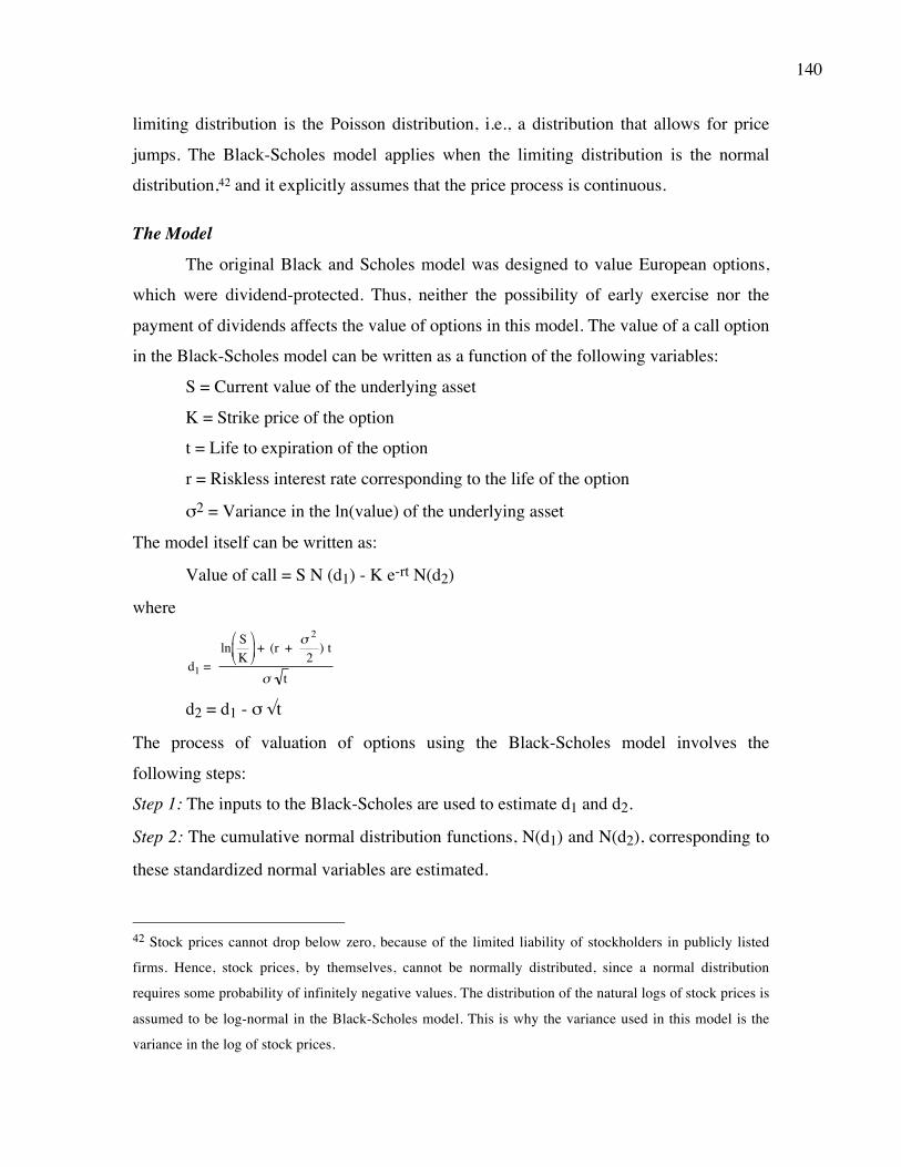
140
limiting distribution is the Poisson distribution, i.e., a distribution that allows for price
jumps. The Black-Scholes model applies when the limiting distribution is the normal
distribution,42 and it explicitly assumes that the price process is continuous.
The Model
The original Black and Scholes model was designed to value European options,
which were dividend-protected. Thus, neither the possibility of early exercise nor the
payment of dividends affects the value of options in this model. The value of a call option
in the Black-Scholes model can be written as a function of the following variables:
S = Current value of the underlying asset
K = Strike price of the option
t = Life to expiration of the option
r = Riskless interest rate corresponding to the life of the option
σ2 = Variance in the ln(value) of the underlying asset
The model itself can be written as:
Value of call = S N (d1) - K e-rt N(d2)
where
€
d1 = ln S
K"
# $
%
& ' + (r + σ
2
2) t
σ t
d2 = d1 - σ √t
The process of valuation of options using the Black-Scholes model involves the
following steps:
Step 1: The inputs to the Black-Scholes are used to estimate d1 and d2.
Step 2: The cumulative normal distribution functions, N(d1) and N(d2), corresponding to
these standardized normal variables are estimated.
42 Stock prices cannot drop below zero, because of the limited liability of stockholders in publicly listed
firms. Hence, stock prices, by themselves, cannot be normally distributed, since a normal distribution
requires some probability of infinitely negative values. The distribution of the natural logs of stock prices is
assumed to be log-normal in the Black-Scholes model. This is why the variance used in this model is the
variance in the log of stock prices.

141
Step 3: The present value of the exercise price is estimated, using the continuous time
version of the present value formulation:
Present value of exercise price = K e-rt
Step 4: The value of the call is estimated from the Black-Scholes model.
The determinants of value in the Black-Scholes are the same as those in the
binomial - the current value of the stock price, the variability in stock prices, the time to
expiration on the option, the strike price, and the riskless interest rate. The principle of
replicating portfolios that is used in binomial valuation also underlies the Black-Scholes
model. In fact, embedded in the Black-Scholes model is the replicating portfolio.
Value of call = S N (d1) - K e-rt N(d2)
Buy N(d1) shares Borrow this amount
N(d1), which is the number of shares that are needed to create the replicating portfolio is
called the option delta. This replicating portfolio is self-financing and has the same value
as the call at every stage of the option's life.
Model Limitations and Fixes
The version of the Black-Scholes model presented above does not take into
account the possibility of early exercise or the payment of dividends, both of which
impact the value of options. Adjustments exist, which while not perfect, provide partial
corrections to value.
1. Dividends
The payment of dividends reduces the stock price. Consequently, call options will
become less valuable and put options more valuable as dividend payments increase. One
approach to dealing with dividends to estimate the present value of expected dividends
paid by the underlying asset during the option life and subtract it from the current value
of the asset to use as “S” in the model. Since this becomes impractical as the option life
becomes longer, we would suggest an alternate approach. If the dividend yield (y =
dividends/ current value of the asset) of the underlying asset is expected to remain
unchanged during the life of the option, the Black-Scholes model can be modified to take
dividends into account.

142
C = S e-yt N(d1) - K e-rt N(d2)
where
€
d1 = ln S
K"
# $
%
& ' + (r - y + σ
2
2) t
σ t
d2 = d1 - σ √t
From an intuitive standpoint, the adjustments have two effects. First, the value of the
asset is discounted back to the present at the dividend yield to take into account the
expected drop in value from dividend payments. Second, the interest rate is offset by the
dividend yield to reflect the lower carrying cost from holding the stock (in the replicating
portfolio). The net effect will be a reduction in the value of calls, with the adjustment,
and an increase in the value of puts.
2. Early Exercise
The Black-Scholes model is designed to value European options, whereas most
options that we consider are American options, which can be exercised anytime before
expiration. Without working through the mechanics of valuation models, an American
option should always be worth at least as much and generally more than a European
option because of the early exercise option. There are three basic approaches for dealing
with the possibility of early exercise. The first is to continue to use the unadjusted Black-
Scholes, and regard the resulting value as a floor or conservative estimate of the true
value. The second approach is to value the option to each potential exercise date. With
options on stocks, this basically requires that we value options to each ex-dividend day
and chooses the maximum of the estimated call values. The third approach is to use a
modified version of the binomial model to consider the possibility of early exercise.
While it is difficult to estimate the prices for each node of a binomial, there is a
way in which variances estimated from historical data can be used to compute the
expected up and down movements in the binomial. To illustrate, if σ2 is the variance in
ln(stock prices), the up and down movements in the binomial can be estimated as
follows:
u = Exp [(r - σ2/2)(T/m) + √(σ2T/m)]

143
d = Exp [(r - σ2/2)(T/m) - √(σ2T/m)]
where u and d are the up and down movements per unit time for the binomial, T is the life
of the option and m is the number of periods within that lifetime. Multiplying the stock
price at each stage by u and d will yield the up and the down prices. These can then be
used to value the asset.
3. The Impact Of Exercise On The Value Of The Underlying Asset
The derivation of the Black-Scholes model is based upon the assumption that
exercising an option does not affect the value of the underlying asset. This may be true
for listed options on stocks, but it is not true for some types of options. For instance, the
exercise of warrants increases the number of shares outstanding and brings fresh cash
into the firm, both of which will affect the stock price.43 The expected negative impact
(dilution) of exercise will decrease the value of warrants compared to otherwise similar
call options. The adjustment for dilution in the Black-Scholes to the stock price is fairly
simple. The stock price is adjusted for the expected dilution from the exercise of the
options. In the case of warrants, for instance:
Dilution-adjusted S = (S ns+W nw) / (ns + nw)
where
S = Current value of the stock nw = Number of warrants
outstanding
W = Market value of warrants outstanding ns = Number of shares outstanding
When the warrants are exercised, the number of shares outstanding will increase,
reducing the stock price. The numerator reflects the market value of equity, including
both stocks and warrants outstanding. The reduction in S will reduce the value of the call
option.
There is an element of circularity in this analysis, since the value of the warrant is
needed to estimate the dilution-adjusted S and the dilution-adjusted S is needed to
estimate the value of the warrant. This problem can be resolved by starting the process
43 Warrants are call options issued by firms, either as part of management compensation contracts or to
raise equity.
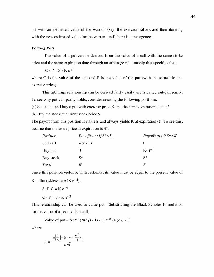
144
off with an estimated value of the warrant (say, the exercise value), and then iterating
with the new estimated value for the warrant until there is convergence.
Valuing Puts
The value of a put can be derived from the value of a call with the same strike
price and the same expiration date through an arbitrage relationship that specifies that:
C - P = S - K e-rt
where C is the value of the call and P is the value of the put (with the same life and
exercise price).
This arbitrage relationship can be derived fairly easily and is called put-call parity.
To see why put-call parity holds, consider creating the following portfolio:
(a) Sell a call and buy a put with exercise price K and the same expiration date "t"
(b) Buy the stock at current stock price S
The payoff from this position is riskless and always yields K at expiration (t). To see this,
assume that the stock price at expiration is S*:
Position Payoffs at t if S*>K Payoffs at t if S*<K
Sell call -(S*-K) 0
Buy put 0 K-S*
Buy stock S* S*
Total K K
Since this position yields K with certainty, its value must be equal to the present value of
K at the riskless rate (K e-rt).
S+P-C = K e-rt
C - P = S - K e-rt
This relationship can be used to value puts. Substituting the Black-Scholes formulation
for the value of an equivalent call,
Value of put = S e-yt (N(d1) - 1) - K e-rt (N(d2) - 1)
where
€
d1 = ln S
K"
# $
%
& ' + (r - y + σ
2
2) t
σ t

145
d2 = d1 - σ √t

146
CHAPTER 8
MODEL CHOICES AND A PHIOSOPHICAL DISCOURSE The problem in valuation is not that there are not enough models to value an asset,
it is that there are too many. Choosing the right model to use in valuation is as critical to
arriving at a reasonable value as understanding how to use the model. This chapter
attempts to provide an overview of the valuation models introduced in this book and a
general framework that can be used to pick the right model for any task. It closes with
some thoughts about valuation in general that are worth keeping in mind, as you start
valuing assets or companies.
Choices in valuation models In the broadest possible terms, firms or assets can be valued in one of four ways –
asset based valuation approaches where you estimate what the assets owned by a firm are
worth currently, discounted cashflow valuation approaches that discount cashflows to
arrive at a value of equity or the firm, relative valuation approaches that base value upon
multiples and option pricing approaches that use contingent claim valuation. Within each
of these approaches, there are further choices that help determine the final value.
There are at least two ways in which you can value a firm using asset based
valuation techniques. One is liquidation value, where you consider what the market will
be willing to pay for assets, if the assets were liquidated today. The other is replacement
cost, where you evaluate how much it would cost you to replicate or replace the assets
that a firm has in place today.
In the context of discounted cashflow valuation, cashflows to equity can be
discounted at the cost of equity to arrive at a value of equity or cashflows to the firm can
be discounted at the cost of capital to arrive at the value for the firm. The cashflows to
equity themselves can be defined in the strictest sense as dividends or in a more
expansive sense as free cashflows to equity. These models can be further categorized on
the basis of assumptions about growth into stable growth, two-stage and three-stage
models. Finally, the measurement of earnings and cashflows may be modified to match
the special characteristics of the firm/asset - current earnings for firms/assets which have
147
normal earnings or normalized earnings for firms/assets whose current earnings may be
distorted either by temporary factors or cyclical effects.
In the context of multiples, you can use either equity or firm value as your
measure of value and relate it to a number of firm-specific variables – earnings, book
value and sales. The multiples themselves can be estimated by using comparable firms in
the same business or from cross-sectional regressions that use the broader universe. For
other assets, such as real estate, the price can similarly expressed as a function of gross
income or per square foot of space. Here, the comparables would be other properties in
the same locale with similar characteristics.
Contingent claim models can also be used in a variety of scenarios. When you
consider the option that a firm has to delay making investment decisions, you can value a
patent or an undeveloped natural resource reserve as an option. The option to expand may
make young firms with potentially large markets trade at a premium on their discounted
cashflow values. Finally, equity investors may derive value from the option to liquidate
troubled firms with substantial debt.
Which approach should you use? The values that you obtain from the four approaches described above can be very
different and deciding which one to use can be a critical step. This judgment, however,
will depend upon several factors, some of which relate to the business being valued but
many of which relate to you, as the analyst.
Asset or Business Characteristics
The approach that you use to value a business will depend upon how marketable
its assets are, whether it generates cash flows and how unique it is in terms of its
operations.
Marketability of Assets
Liquidation valuation and replacement cost valuation are easiest to do for firms
that have assets that are separable and marketable. For instance, you can estimate the
liquidation value for a real estate company because its properties can be sold individually
and you can estimate the value of each property easily. The same cannot be said of
148
companies like Coca Cola or Disney, which have valuable assets that are linked to each
other or to a brand name. You can also use this same analysis to see why the liquidation
or replacement cost value of a high growth business will bear little resemblance to true
value. Unlike assets in place, growth assets cannot be easily identified or sold.
Cash Flow Generating Capacity
You can categorize assets into three groups based upon their capacity to generate
cash flows – assets that are either generating cash flows currently or are expected to do so
in the near future, assets that are not generating cash flows currently but could in the
future in the event of a contingency and assets that will never generate cash flows.
• The first group includes most publicly traded companies and these firms can be
valued using discounted cash flow models. Note that we do not draw a distinction
between negative and positive cash flows and young, start-up companies that
generate negative cash flow can still be valued using discounted cash flow
models.
• The second group includes assets such as drug patents, promising (but not viable)
technology, undeveloped oil or mining reserves and undeveloped land. These
assets may generate no cash flows currently and could generate large cash flows
in the future but only under certain conditions – if the FDA approves the drug
patent, if the technology becomes commercially viable, if oil prices and
commercial property values go up. While you could estimate expected values
using discounted cash flow models by assigning probabilities to these events, you
will understate the value of the assets if you do so. You should value these assets
using option pricing models.
• Assets that are never expected to generate cash flows include your primary
residence, a baseball card collection or fine art. These assets can only be valued
using relative valuation models.
Uniqueness (or presence of comparables)
In a market where thousands of stocks are traded and tens of thousands of assets
are bought and sold every day, it may be difficult to visualize an asset or business that is
so unique that you cannot find comparable assets. On a continuum, though, some assets

149
and businesses are part of a large group of similar assets, with no or very small
differences across the assets. These assets are tailor-made for relative valuation, since
assembling comparable assets (businesses) and controlling for differences is simple. The
further you move from this ideal, the less reliable is relative valuation. For businesses that
are truly unique, discounted cash flow valuation will yield much better estimates of
value.
Analyst Characteristics and Beliefs
The valuation approach that you choose to use will depend upon your time
horizon, the reason that you are doing the valuation in the first place and what you think
about markets – whether they are efficient and if they are not, what form the inefficiency
takes.
Time Horizon
At one extreme, in discounted cash flow valuation you consider a firm as a going
concern that may last into perpetuity. At the other extreme, with liquidation valuation,
you are estimating value on the assumption that the firm will cease operations today.
With relative valuation and contingent claim valuation, you take an intermediate position
between the two. Not surprisingly, then, you should be using discounted cash flow
valuation, if you have a long time horizon, and relative valuation, if you have a shorter
time horizon. This may explain why discounted cash flow valuation is more prevalent in
valuing a firm for an acquisition and relative valuation is more common in equity
research and portfolio management.
Reason for doing the valuation
Analysts value businesses for a number of reasons and the valuation approach
used will vary depending upon the reason. If you are an equity research analyst following
steel companies, your job description is simple. You are asked to find the most under and
over valued companies in the sector and not to take a stand on whether the sector overall
is under or over valued. You can see why multiples would be your weapon of choice
when valuing companies. This effect is likely to be exaggerated if the way you are judged

150
and rewarded is on a relative basis, i.e., your recommendations are compared to those
made by other steel company analysts. If you are an individual investor setting money
aside for retirement or a private businessperson valuing a business for purchase, on the
other hand, you want to estimate intrinsic value. Consequently, discounted cash flow
valuation is likely to be more appropriate for your needs.
Beliefs about Markets
Embedded in each approach are assumptions about markets and how they work or
fail to work. With discounted cash flow valuation, you are assuming that market prices
deviate from intrinsic value but that they correct themselves over long periods. With
relative valuation, you are assuming that markets are on average right and that while
individual firms in a sector or market may be mispriced, the sector or overall market is
fairly priced. With asset-based valuation models, you are assuming that the markets for
real and financial assets can deviate and that you can take advantage of these differences.
Finally, with option pricing models, you are assuming that markets are not very efficient
at assessing the value of flexibility that firms have and that option pricing models will
therefore give you an advantage. In each and every one of these cases, though, you are
assuming that markets will eventually recognize their mistakes and correct them.
Choosing the right DCF Model The model used in valuation should be tailored to match the characteristics of the
asset being valued. The unfortunate truth is that the reverse is often true. Time and
resources are wasted trying to make assets fit a pre-specified valuation model, either
because it is considered to be the 'best' model or because not enough thought goes into
the process of model choice. There is no one 'best' model. The appropriate model to use
in a particular setting will depend upon a number of the characteristics of the asset or firm
being valued.
Firm versus Equity Valuation
With consistent assumptions about growth and leverage, you should get the same
value for your equity using the firm approach (where you value the firm and subtract
outstanding debt) and the equity approach (where you value equity directly). If this is the
151
case, you might wonder why you would pick one approach over the other. The answer is
purely pragmatic and tilts us towards firm valuation, over equity valuation, for most
firms:
(1) For most publicly traded firms, it is not only easier to estimate cash flows prior to
debt payments and to adjust the discount rate for risk (or compute the tax benefits of debt
separately) but it also preserves more flexibility. In other words, you can go back and
change your assumptions about debt usage in the future easily in a firm valuation, but it is
far more difficult to do in equity valuation
(2) By separating operating assets from non-operating assets (cash, cross holdings), firm
valuation allows us to focus on the risk and cash flow characteristics of the business
decisions made by a firm. While you do have to take care to bring in the value of cash
and cross holdings into the final value, you can value these investments using much
simpler techniques than you use for the operating assets.
Are there dangers? Sure. By focusing on cash flows prior to debt payments, you may be
missing signals that the firm may be headed towards default. However, there is no reason
why you cannot value a firm using firm valuation approaches and estimate the cash flow
for equity separately.
So, when should you use equity valuation? For financial service firms, where debt
is both difficult to define and determine and where it is more raw material than a source
of capital, the focus should stay firmly on equity valuation. For real estate or private
equity investments, where the focus is on highly levered equity investors and their
returns, it may also be useful to focus on the equity invested and the cash flows to these
equity investors.
Cost of Capital versus APV valuation In the chapter on APV valuation, we noted that the cost of capital approaches and
APV will yield the same value for a business, with consistent assumptions on growth and
risk. The key difference between the approaches is that the tax benefits of debt are
incorporated into the discount rate (cost of capital) in the cost of capital approach and are
counted separately, net of bankruptcy costs, in the APV approach. Again, the choice has
to be a pragmatic one:

152
a. For companies where the debt ratio is expected to change over time, it is easier to
adjust the cost of capital for time varying debt ratios than it is to estimate the net
value added by debt.
b. In transactions where the focus is on dollar debt and changes in that value over
time, the APV approach is easier to use. Estimating debt ratios in future periods
can be problematic, with dollar debt values, because estimating equity values in
future periods puts you at risk of circularity in the valuation.
Even in the latter case, a key input into the APV model is the expected bankruptcy
cost. If it is difficult to estimate bankruptcy costs, analysts often ignore these costs
and the values obtained from APV models have to be taken with a grain of salt, since
they will be overstated.
Dividends or Free Cash flow to Equity In valuing equity, you can discount dividends or free cashflows to equity. In the
chapter on equity valuation models, we examined why the models may give you different
answers, and what you would need to assume for the models to reconcile. If you can
estimate the free cash flow to equity (the potential dividend), you will get a more realistic
estimate of value using it to compute value rather than the dividends. In effect, for a firm
that pays too little in dividends (relative to its free cash flow to equity), you are
incorporating the effect of the cash build up in the firm into the value of equity. For a
firm that pays out too much in dividends, you are reducing the value of equity to reflect
your expectation that the dividends are unsustainable.
In some cases, though, especially with financial service companies, it may be
difficult, if not impossible, to estimate the free cash to equity, because capital
expenditures and working capital are not identifiable easily. In those cases, you have no
choice but to focus on the dividend discount model.
Choosing the Right Relative Valuation Model Many analysts choose to value assets using relative valuation models. In making
this choice, two basic questions have to be answered -- Which multiple will be used in
the valuation? Will this multiple be arrived at using the sector or the entire market?

153
Which multiple should I use?
In the chapters on multiples, we presented a variety of multiples. Some were
based upon earnings, some on book value and some on revenues. For some multiples, we
used current values and for others, we used forward or forecast values. Since the values
you obtain are likely to be different using different multiples, deciding which multiple to
use can make a big difference to your estimate of value. There are three ways you can
answer this question –the first is to adopt the cynical view that you should use the
multiple that reflects your biases, the second is to value your firm with different multiples
and try to use all of the values that you obtain and the third is to pick the best multiple
and base your valuation on it.
The most sensible choice is to pick a multiple that resonates in the sector that your
company operates in. One way to find this multiple is to look at the variables that
managers in the sector focus and work backwards to the multiple that matches that
variable. In retailing, for instance, the focus on margins and same store sales would lead
us to use revenue multiples. In banking, the emphasis on return on equity would suggest
that price to book ratios be used to value banks. The other is to find the variable that is
most highly correlated with firm value in the sector. For instance, current earnings and
value are much more highly correlated in consumer product companies than in
technology companies. Using price earnings ratios makes more sense for the former than
for the latter.
How should you define comparable companies?
There are three choices. One is to define comparable narrowly and to look for
companies that resemble the company that you are valuing on multiple dimensions – size,
growth potential and risk. The net result will be a small sample of firms that are
“similar” to the firm you are valuing. The second is to define comparable firms more
broadly, and to bring in firms that operate in the same sector, even if they differ from
your firm on key dimensions. This will allow for much larger samples of firms, albeit
some with different characteristic than the firm you are valuing.
If you want to compare the pricing multiple (PE, EV/EBITDA) that your firm is
trading at to an average or median value, not correcting for differences across companies,

154
you should go with the former: a small sample of similar companies. The risk, though, is
that you may be finding a small cluster of mispriced companies. If you plan to control for
differences across firms – by modifying the multiple or with a regression- you will be
better served with a larger sample of less comparable firms.
Intrinsic versus Relative Value
The two approaches to valuation – discounted cash flow valuation and relative
valuation – will generally yield different estimates of value for the same firm at the same
point in time. It is even possible for one approach to generate the result that the stock is
under valued while the other concludes that it is over valued. Furthermore, even within
relative valuation, we can arrive at different estimates of value depending upon which
multiple we use and what firms we based the relative valuation on.
The differences in value between discounted cash flow valuation and relative
valuation come from different views of market efficiency, or put more precisely, market
inefficiency. In discounted cash flow valuation, we assume that markets make mistakes,
that they correct these mistakes over time, and that these mistakes can often occur across
entire sectors or even the entire market. In relative valuation, we assume that while
markets make mistakes on individual stocks, they are correct on average. In other words,
when we value a new software company relative to other small software companies, we
are assuming that the market has priced these companies correctly, on average, even
though it might have made mistakes in the pricing of each of them individually. Thus, a
stock may be over valued on a discounted cash flow basis but under valued on a relative
basis, if the firms used for comparison in the relative valuation are all overpriced by the
market. The reverse would occur, if an entire sector or market were underpriced.
When should you use the option pricing models? In the chapters on applying option pricing models to valuation, we presented a
number of scenarios where option pricing may yield a premium on traditional discounted
cash flow valuation. We do not intend to revisit those scenarios, but offer the following
general propositions that you should keep in mind when using option pricing models.
155
• Use Options sparingly: Restrict your use of options to where they make the
biggest difference in valuation. In general, options will affect value the most at
smaller firms that derive the bulk of their value from assets that resemble options.
Therefore, valuing patents as options to estimate firm value makes more sense for
a small biotechnology firm than it does for a drug giant like Merck. While Merck
may have dozens of patents, it derives much of its value from a portfolio of
developed drugs and the cash flows they generate.
• Opportunities are not always options: You should be careful not to mistake
opportunities for options. Analysts often see a firm with growth potential and
assume that there must be valuable options embedded in the firm. For
opportunities to become valuable options, you need some degree of exclusivity
for the firm in question – this can come from legal restrictions on competition or a
significant competitive edge.
• Do not double count options: All too often, analysts incorporate the effect of
options on fundamentals in the company value and then proceed to add on
premiums to reflect the same options. Consider, for instance, the undeveloped oil
reserves owned by an oil company. While it is legitimate to value these reserves
as options, you should not add this value to a discounted cashflow valuation of the
company, if your expected growth rate in the valuation is set higher because of
the firm’s undeveloped reserves.
Some fundamental (philosophical) propositions about valuation When confronted with uncertainty or missing information, we are tempted to
adopt loosely backed rules of thumb and make inconsistent assumptions about growth,
risk, and cash flows. The following sections outline a few propositions that can guide us
in making better judgments and estimates, and result in better valuations.
Proposition 1: Be steadfast on principles, open to new tools and flexible on estimates.
A principle is a core idea, a tool is what you use to put that idea into practice, and an
estimate is what emerges from that tool. There are a few basic principles in valuation that
we should never compromise on, no matter what the counterarguments are. They include
the following (a) that an asset derives it value from its capacity to generate cash flows in

156
the future, (b) that risk affects value ,(c) that growth has to be earned (not endowed) and
(d) that the laws of demand and supply cannot be repealed. An analyst who argues that
firms can grow forever without reinvesting is violating a first principle. Lest this be seen
as a sign of rigidity, we would hasten to add that we should always be willing to
compromise on, and accept, better tools, and be open to alternative estimates for inputs
into value.
Proposition 2: Pay Heed to Markets, But Don’t Let Them Determine Your Valuations
Many of the companies that we are called on to value are traded in financial markets and
have market prices. Without making any judgments about markets or their efficiency, we
believe that there is valuable information in how the market is pricing assets. When
valuing a company, we should pay attention to the market price for two reasons:
• The information we extract from markets on implied growth rates, risk, and cash
flows can be used to improve our valuations.
• Ultimately, we make money not from our estimates of intrinsic values, but from the
market prices moving to those intrinsic values. Thus, we need to understand why
market prices deviate from value and how they will adjust over time.
At the same time, paying too much attention to markets (and prices) can lead to paralysis,
since there is always an alternative set of assumptions under which the market price is
justified. In other words, if we start by assuming that the market is always right, we will
end up confirming that assumption in our valuations.
Proposition 3: Risk Matters
It is true that considerable resources have been invested in both academia and practice in
coming up with models to assess risk and derive expected returns. It is also true that these
models often make assumptions about the real world that do not withstand close scrutiny.
In the capital asset pricing model, for instance, we assume no transaction costs and
private information to derive the relationship between expected returns and betas.
Analysts, looking at these models, find themselves disagreeing with the assumptions.
That is perfectly understandable, but jumping from that disagreement to a conclusion that
risk does not matter in value is not.
Proposition 4: Growth Is Not Free and Is Not Always Value-Adding

157
If there is a theme to our discussions of growth across the chapters, it is that growth is not
free. Ultimately, the expected growth in a company’s earnings and cash flows must come
from either new investments or improved efficiency. The latter is finite growth and there
is a limit to how efficient you can become as a firm, whereas new investment growth can
be for the long term (and potentially forever). It is also critical to remember that growth
by itself is not always a plus for a company, since the value added by growth is a function
of the quality of the investments that generated that growth.
Proposition 5: All Good Things Come to an End
In addition to looking at the value added or destroyed by growth, we often have to make
estimates of future growth rates for companies. In making this assessment, we must pay
attention to two key variables. The first is the scaling effect. As companies get bigger, it
becomes more and more difficult for them to keep delivering the excess returns and
growth rates they did in the past. Thus, it is almost a certainty that a firm that has grown
100% a year for the last three years will grow at a slower rate in the next three years. The
second factor is competition. When firms are successful, they attract attention, which in
turn leads to imitation and increased competition. While firms may be successful at
keeping this competition at bay for extended periods (using legal and other tools), the
new competitors will inevitably chip away at profitability and growth.
Proposition 6: Watch Out for Truncation Risk
In conventional discounted cash flow valuation, we value firms as going concerns, with
cash flows continuing into perpetuity. While this may not be an unreasonable assumption
for some firms, the reality is that most firms do not make it to this stable-growth phase.
Many young firms run out of cash and have to shut down, some mature firms become the
targets of acquirers, and most distressed firms end up defaulting on debt and going out of
business. The optimism that underlies discounted cash flow valuation can lead us to
overestimate the values of firms, where the risk of not making it (truncation risk) is high.
Proposition 7: Look at the Past, But Think About the Future
One of the conundrums we face in valuation is that although almost all the data we have
available to us is about the past, reflecting the company’s history (past financial
statements, betas), the sector (industry average margins and returns on capital), and
macroeconomic variables (interest rates, exchange rates, stock returns), all the forecasts

158
we have to make are for the future. While we cannot manufacture data for the future, we
can follow some simple rules to minimize the damage. First, use historical data, but do
not be bound by it. Second, trust in mean reversion, but watch out for structural breaks
and challenges. Third, use forward estimates as alternatives or checks to historical data.
Proposition 8: Draw on the Law of Large Numbers
In many cases, the numbers that we use in valuation come from looking at samples of
past data. The historical equity risk premium, for instance, is estimated by averaging the
premium earned by stocks over treasuries over long time periods. Even if these estimates
are constantly updated and are from services that have impeccable reputations, these
numbers cannot be treated as facts. They are estimates, based on samples, and they come
with substantial standard errors. While making estimates based on data will always be
subject to noise, we can do some things to make these estimates more precise. The first is
to use larger samples. With historical risk premiums, for instance, an equity risk premium
estimated over 100 years of data will have a standard error of only 2% associated with it.
With betas, replacing a single regression beta with a sector average can yield far more
precision in your estimate. The second is to use statistical tools, like multiple regressions,
to reduce the estimation error. We should make a final point about the law of large
numbers. Since the values we obtain for individual companies are estimates, the
likelihood that we will be wrong about any one company in any one period is high.
However, if we assess value well, our chances of being right will improve if we extend to
multiple periods (longer time horizons) and across multiple stocks (portfolios).
Proposition 9: Accept Uncertainty, and Deal with It
Accept uncertainty as a given, understanding that no matter how carefully we construct
models, we cannot make uncertainty go away. Thus, adding more detail to models or
making models more complicated, both of which are tactics that analysts use to reduce
uncertainty, often does little to alleviate the problem and may actually make it worse.
Uncertainty and risk are part of life and investing. When valuing companies, we can
demand a premium for taking this risk in the discount rate and arrive at a risk-adjusted
value, but it will change as circumstances change.
Proposition 10: Convert Stories to Numbers

159
One of the critiques of discounted cash flow valuation is that it is so focused on numbers
that it misses the qualitative variables. Included in the list of qualitative variables are
items such as customer loyalty, brand name, and good management. Every number in a
discounted cash flow valuation should have an economic rationale[md]a good economic
story behind it. Thus, when we set a firm’s return on capital at 15%, well above its cost of
capital, it behooves us to think about this firm’s competitive advantages (most of which
are qualitative) and how they translate into the return on capital. On the flip side, every
solid economic story should find a place in the numbers. Brand name affects value, but it
does so by increasing margins and excess returns, not as a premium at the end of the
process.
Conclusion The analyst faced with the task of valuing a firm/asset or its equity has to choose
among three different approaches -- discounted cashflow valuation, relative valuation and
option pricing models; and within each approach, they must also choose among different
models. These choices will be driven largely by the characteristics of the firm/asset being
valued - the level of its earnings, its growth potential, the sources of earnings growth, the
stability of its leverage and its dividend policy. Matching the valuation model to the asset
or firm being valued is as important a part of valuation as understanding the models and
having the right inputs.

160
Top Related