Download - The selling process: If at first you don't succeed, try try try …economics.uwo.ca/grad/alumniconference2005/Papers/anglin.pdf · The selling process: If, at first, you don't succeed,

The selling process: If, at first, you don'tsucceed, try, try, try again

By Paul M. Anglin University of Windsor

July 2004

Abstract

About 40 percent of attempts to sell a house end with the seller not selling. This aspect of behavior has not been studied carefully and, by organizing the datain a way that reveals the behavior of sellers instead of listings, I consider somehypotheses related to the ability of a market process to efficiently allocateresources. First, a change in market conditions may cause the seller to changetheir decision between the time of listing and the end date. Second, the seller mayenter the market as a test and find that the buyers’ willingness-to-pay is less thantheir willingness-to-accept. Third, the seller may end a listing because they aredissatisfied with a broker and wish to switch to a new broker. There is somesupport for each hypothesis.

JEL: C78, D80, R31, C41, D81, D83 Keywords: real estate, bargaining, market frictions, relist, real estate agent, list price,

over-pricing, selling price, liquidity, bargaining power, search, matching,time-till-sale

This research uses historical data. Anybody using this research should consult a qualifiedprofessional since neither I nor the University of Windsor will accept any responsibility for costsor consequences associated with this research. Thanks are due to Dinghai Xu, Shi Fu and YangWang for their able research assistance. Robin Wiebe’s assistance with data and insights hasalso been useful, though he does not bear any responsibility for errors and omissions. Commentswould be appreciated and can be sent to [email protected] or by mail to the Department ofEconomics, University of Windsor, Windsor, ON Canada N9B 3P4. The latest version of thispaper can be found at http://www.uwindsor.ca/PaulAnglin

Try, try and try again 1Economists like to argue that the price system rations the set of potential buyers and

sellers so that the most willing sellers trade with the most willing buyers. In this model, it is

difficult to understand why 40 percent of people who attempt to sell their house exit from the

market before selling. Some people give up, which suggests that the market is sending the

wrong signals and wasting scarce resources. Some people start trying to sell again, which

suggests that some real estate agents are not doing a good enough job. These examples imply

that traditional models of the selling process omit important margins of adjustment.

The textbook model of the selling process can be criticized for many reasons, especially

in the context of a housing market. First, it is so costly to sell a house and the commonly

available information is so poor that professionals are often paid to assist most attempts. Even

with their assistance, the process takes many months. Second, theoretical models of the market

process tend to focus on the equilibrium outcome. Given the time needed to sell a house,

variations in this process are likely to have real effects even before a market attains an

equilibrium. Third, many papers study the selling process but only a complementary study of

failures could explain why a sale represents a successful outcome rather than being the only

outcome.

A study of failed attempts reveals new dimensions of behavior such as trying again and

waiting between attempts. The central question is what might cause an attempt to fail. The most

obvious explanation is that market conditions may change but previous research has identified

certain puzzles. Abundant evidence (e.g. Steele, 1996; Mayer and Genesove 1997; Mayer and

Genesove, 2001) suggests that selling prices and list prices adjust surprisingly slowly to even

large changes in the apparent market equilibrium. Other research (Clayton, 1996, 1997;

Capozza, Hendershott and Mack, 2004) shows that housing markets are not informationally

efficient over time. Thus, it may be true that an action that was rational may become irrational

but the constraints that make a choice rational also need to be carefully considered.

Researchers have studied parts of this problem. For example, a poorly informed seller

may also be learning about market conditions during the listing. Such sellers should start with a

Try, try and try again 2high list price as part of an exercise in optimal learning or to allow for the possibility that market

conditions may improve (Read, 1988; Krainer, 2001). Given the benefits associated with such

activities, a few sellers may enter a market with the intention of speculating on future trends or

on luck in the matching process rather than with the intention of selling with probability 1.

A second explanation is simply that a seller’s problem is not stationary (Lambson,

McQueen and Slade, 2003; Ben-Shahar, 2002, Salant, 1991). For example, the cost of selling

may change when they commit to buy a different house. Or, it may be getting close to the start

date for a new job in another city and their children may prefer to start at their new school on

time. Or, the marginal return to remaining on the market may diminish if the house acquires a

stigma (Taylor, 1999).

A third conjecture is related to a weakness of commonly-used data sets. A listing may

end without a sale because the seller is unhappy with one agent and seeks a different agent. If

the second agent is successful then, according to most data sets used to study the selling process,

only the second attempt would be recorded even if the first attempt was also relevant to the

seller. The final hypothesis is that a failure is the fault of the seller. The most obvious action is

the seller’s choice of list price although previous analyses have considered only the effect of the

list price on the length of time it takes to sell a house. As this paper notes, the inference drawn

from an increase in the average time-till-sale and the inference drawn from a decrease in the

probability of expiry differ slightly: the first fact suggests that market conditions are worsening

while the second fact may suggest that sellers see no better alternative. Commonly reported

measures of the state of a market mix these two facts together.

The next section describes the data on failed attempts to sell since this phenomenon is not

well-known. The fact that the data span three years enables me to distinguish first attempts and

second attempts with a reasonable level of confidence. Amongst other facts, I note how the

description of the house usually changes between attempts. The following section offers more

details on the hypotheses concerning seller behavior. In general, I add to the approach outlined

in Anglin, Rutherford and Springer (2003) and Anglin (2004). The third section describes the

Try, try and try again 3

1 Condominium properties, which are distinguished by suite numbers at a single streetaddress, and listings, such as “LOT 23”, were excluded from this study because the data cannotprecisely identify an individual seller. Similarly, property that was “under construction” or“newly constructed” was omitted since the trade offs involved in selling such houses are likely todiffer substantially from other types of property: very few sellers of these properties made a“second attempt”. Properties with a list price above C$450,000 or below C$40,000 or withomitted data in other variables were also excluded.

data and how certain variables were constructed. Where previous papers have tended to

organize the data in a way that focuses on the process of selling a listing, this paper focuses on

the process of selling a house at a specific address. The fourth section discusses some

econometric issues and the fifth section discusses the results. In general, the results support the

hypotheses outlined above.

1/ Introduction to the Data

I use data provided by the Windsor and Essex County Real Estate Board. It represents

24,939 listings of residential1 properties between 1997 and early 2000. Knowing the address and

outcome of each attempt, it is possible to link a sequence of different attempts to sell by one

seller and to distinguish that sequence from one sale followed by an attempt to sell by the

different owner. In total, the data record attempts to sell by 20,002 different sellers.

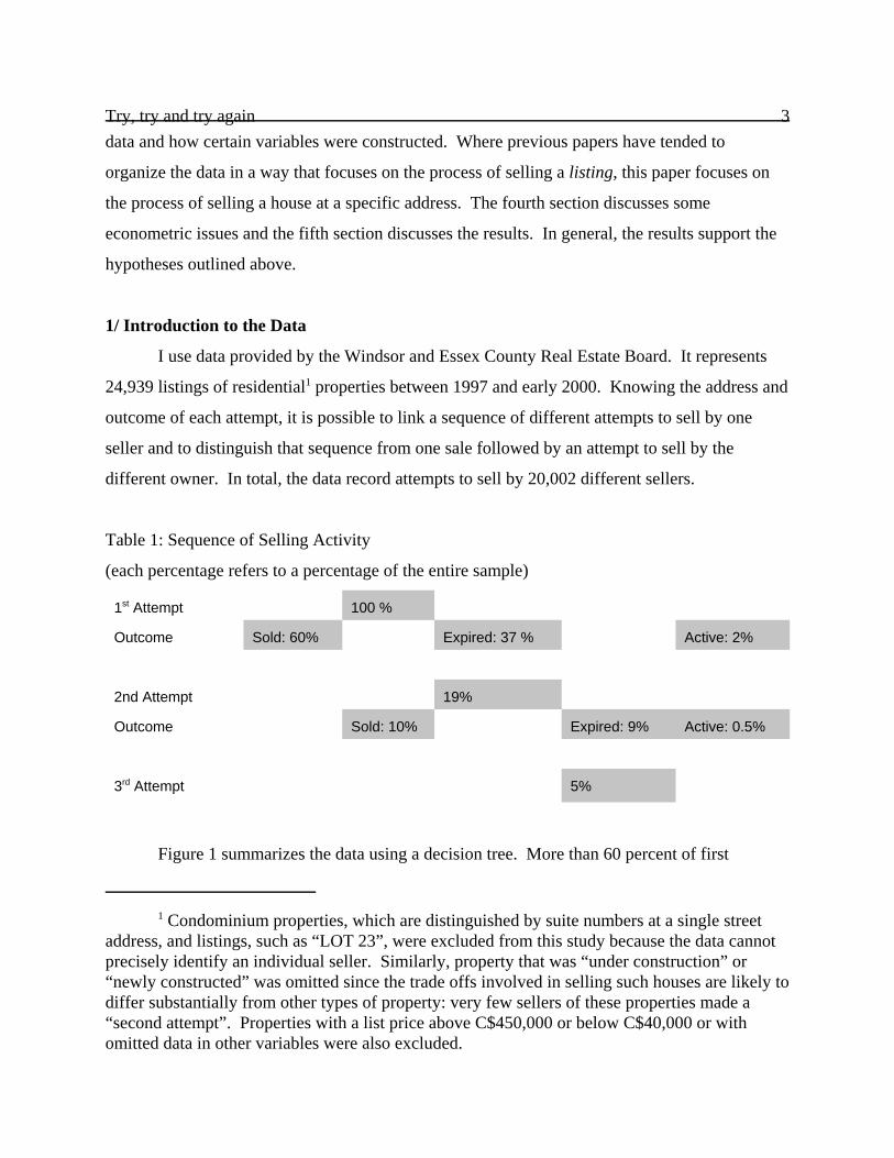
Table 1: Sequence of Selling Activity

(each percentage refers to a percentage of the entire sample)

1st Attempt 100 %

Outcome Sold: 60% Expired: 37 % Active: 2%

2nd Attempt 19%

Outcome Sold: 10% Expired: 9% Active: 0.5%

3rd Attempt 5%

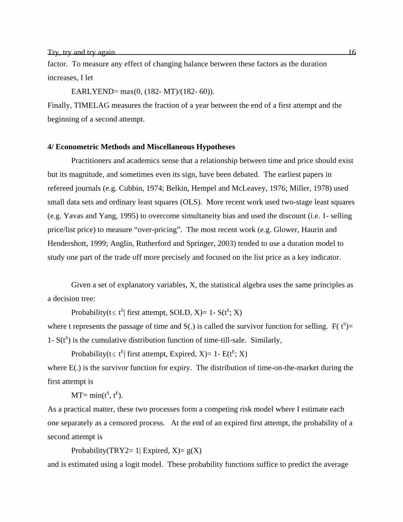
Figure 1 summarizes the data using a decision tree. More than 60 percent of first


0%

5%

10%

15%

20%

Per-w

eek

Prob

.

1 6 11 16 21 26 31Weeks

SOLD EXPD

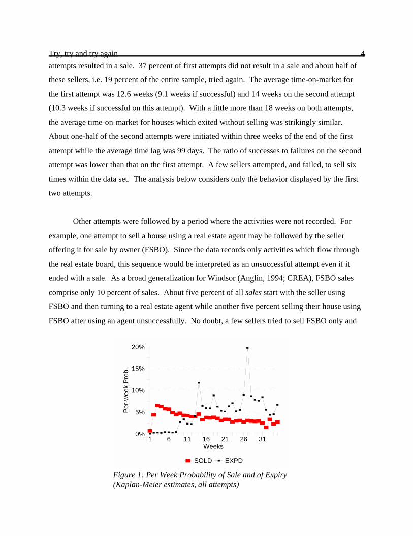
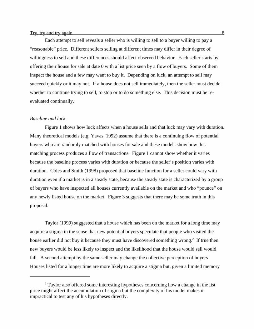
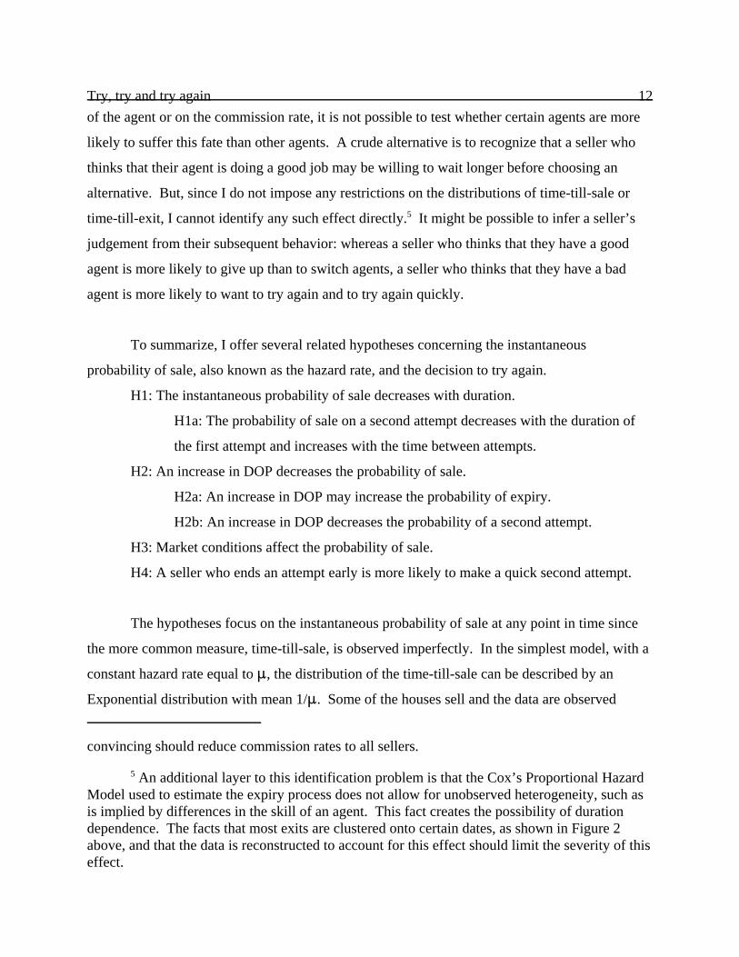
Figure 1: Per Week Probability of Sale and of Expiry(Kaplan-Meier estimates, all attempts)

attempts resulted in a sale. 37 percent of first attempts did not result in a sale and about half of

these sellers, i.e. 19 percent of the entire sample, tried again. The average time-on-market for

the first attempt was 12.6 weeks (9.1 weeks if successful) and 14 weeks on the second attempt

(10.3 weeks if successful on this attempt). With a little more than 18 weeks on both attempts,

the average time-on-market for houses which exited without selling was strikingly similar.

About one-half of the second attempts were initiated within three weeks of the end of the first

attempt while the average time lag was 99 days. The ratio of successes to failures on the second

attempt was lower than that on the first attempt. A few sellers attempted, and failed, to sell six

times within the data set. The analysis below considers only the behavior displayed by the first

two attempts.

Other attempts were followed by a period where the activities were not recorded. For

example, one attempt to sell a house using a real estate agent may be followed by the seller

offering it for sale by owner (FSBO). Since the data records only activities which flow through

the real estate board, this sequence would be interpreted as an unsuccessful attempt even if it

ended with a sale. As a broad generalization for Windsor (Anglin, 1994; CREA), FSBO sales

comprise only 10 percent of sales. About five percent of all sales start with the seller using

FSBO and then turning to a real estate agent while another five percent selling their house using

FSBO after using an agent unsuccessfully. No doubt, a few sellers tried to sell FSBO only and


0

10

20

30

40

50

Perc

ent

1 6 11 16 21 26 31Day of the Month

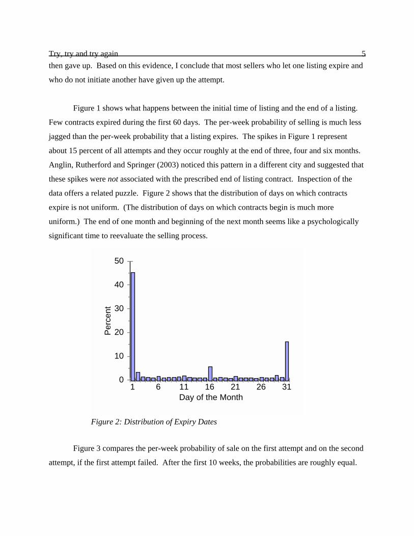
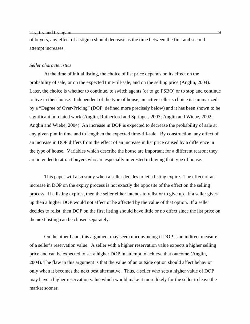
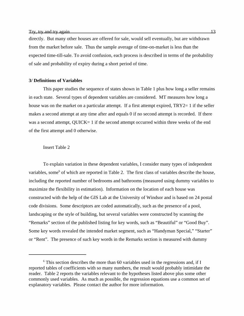
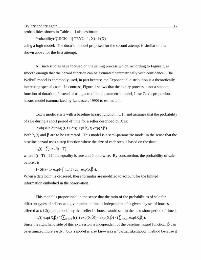
Figure 2: Distribution of Expiry Dates

then gave up. Based on this evidence, I conclude that most sellers who let one listing expire and

who do not initiate another have given up the attempt.

Figure 1 shows what happens between the initial time of listing and the end of a listing.

Few contracts expired during the first 60 days. The per-week probability of selling is much less

jagged than the per-week probability that a listing expires. The spikes in Figure 1 represent

about 15 percent of all attempts and they occur roughly at the end of three, four and six months.

Anglin, Rutherford and Springer (2003) noticed this pattern in a different city and suggested that

these spikes were not associated with the prescribed end of listing contract. Inspection of the

data offers a related puzzle. Figure 2 shows that the distribution of days on which contracts

expire is not uniform. (The distribution of days on which contracts begin is much more

uniform.) The end of one month and beginning of the next month seems like a psychologically

significant time to reevaluate the selling process.

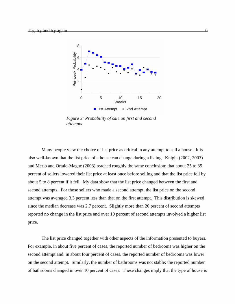
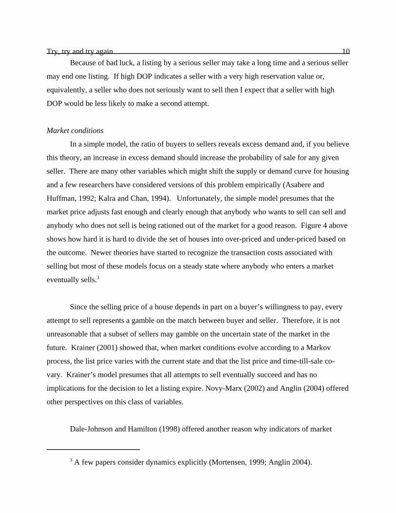
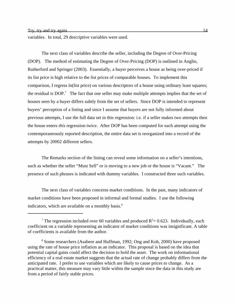
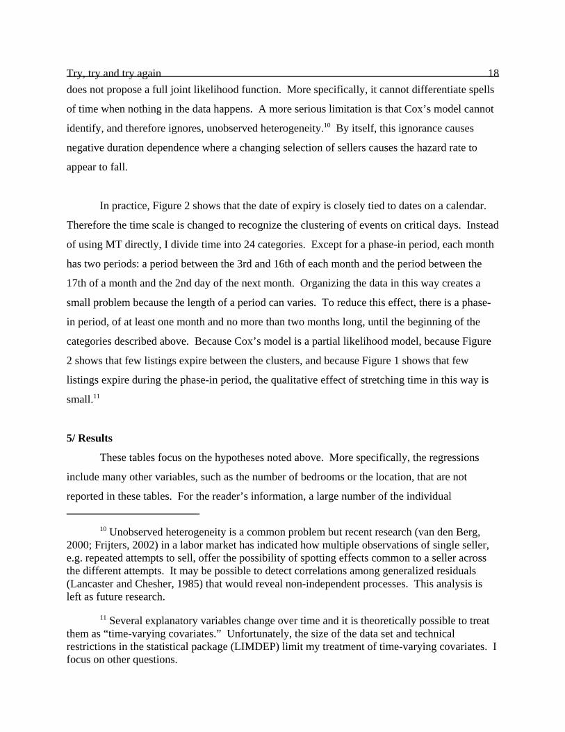
Figure 3 compares the per-week probability of sale on the first attempt and on the second

attempt, if the first attempt failed. After the first 10 weeks, the probabilities are roughly equal.


2

4

6

8

Per-w

eek

Prob

abilit

y

0 5 10 15 20Weeks

1st Attempt 2nd Attempt

Figure 3: Probability of sale on first and secondattempts

Many people view the choice of list price as critical in any attempt to sell a house. It is

also well-known that the list price of a house can change during a listing. Knight (2002, 2003)

and Merlo and Ortalo-Magne (2003) reached roughly the same conclusion: that about 25 to 35

percent of sellers lowered their list price at least once before selling and that the list price fell by

about 5 to 8 percent if it fell. My data show that the list price changed between the first and

second attempts. For those sellers who made a second attempt, the list price on the second

attempt was averaged 3.3 percent less than that on the first attempt. This distribution is skewed

since the median decrease was 2.7 percent. Slightly more than 20 percent of second attempts

reported no change in the list price and over 10 percent of second attempts involved a higher list

price.

The list price changed together with other aspects of the information presented to buyers.

For example, in about five percent of cases, the reported number of bedrooms was higher on the

second attempt and, in about four percent of cases, the reported number of bedrooms was lower

on the second attempt. Similarly, the number of bathrooms was not stable: the reported number

of bathrooms changed in over 10 percent of cases. These changes imply that the type of house is


-0.3 -0.2 -0.1 0 0.1 0.2 0.3 0.4DOP

102030405060708090

Perc

entil

e

Sold Expired

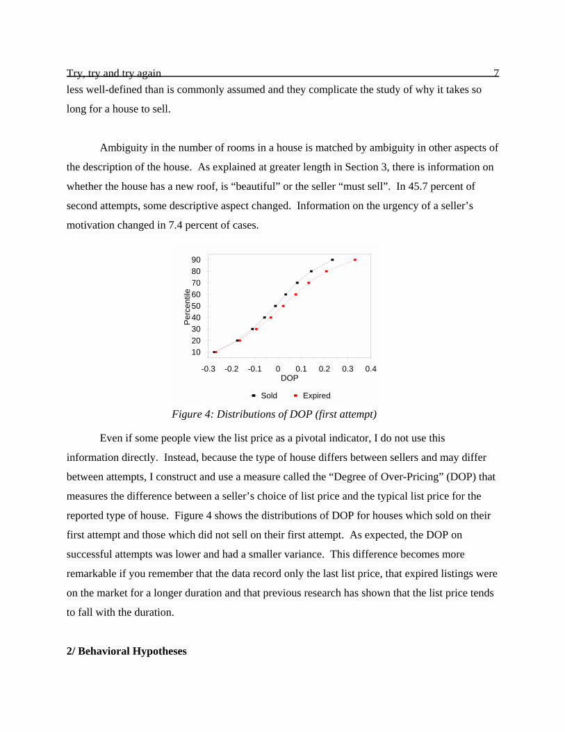
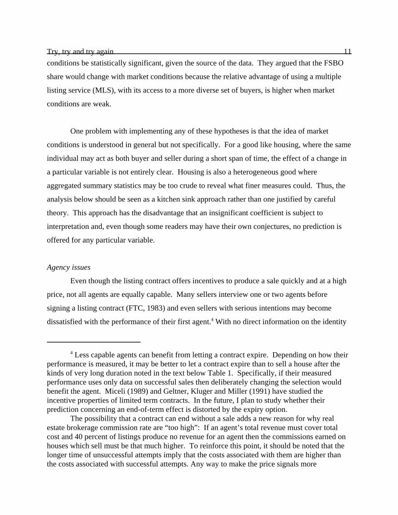
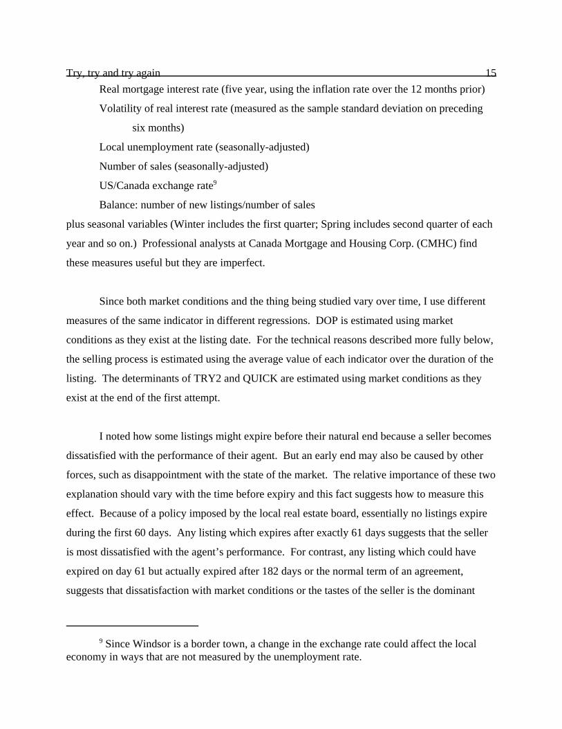
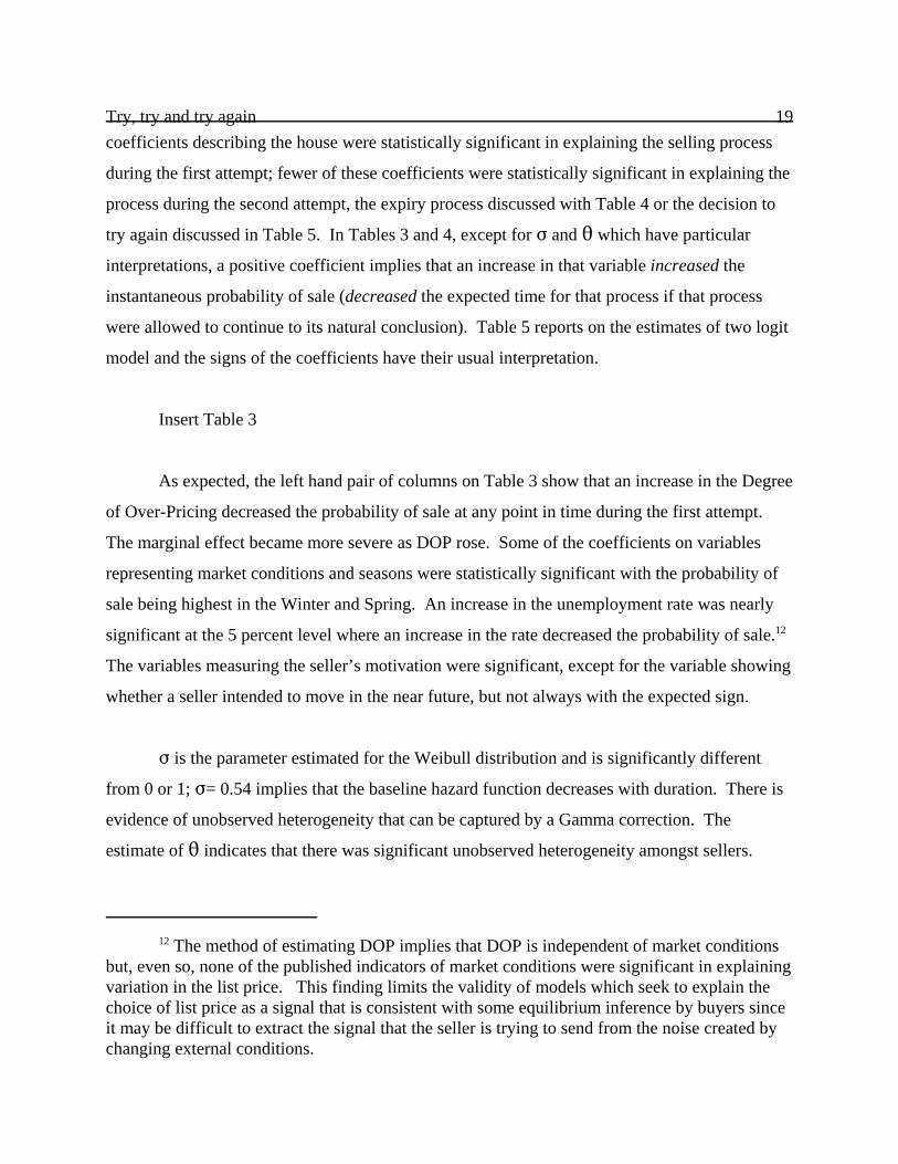
Figure 4: Distributions of DOP (first attempt)

less well-defined than is commonly assumed and they complicate the study of why it takes so

long for a house to sell.

Ambiguity in the number of rooms in a house is matched by ambiguity in other aspects of

the description of the house. As explained at greater length in Section 3, there is information on

whether the house has a new roof, is “beautiful” or the seller “must sell”. In 45.7 percent of

second attempts, some descriptive aspect changed. Information on the urgency of a seller’s

motivation changed in 7.4 percent of cases.

Even if some people view the list price as a pivotal indicator, I do not use this

information directly. Instead, because the type of house differs between sellers and may differ

between attempts, I construct and use a measure called the “Degree of Over-Pricing” (DOP) that

measures the difference between a seller’s choice of list price and the typical list price for the

reported type of house. Figure 4 shows the distributions of DOP for houses which sold on their

first attempt and those which did not sell on their first attempt. As expected, the DOP on

successful attempts was lower and had a smaller variance. This difference becomes more

remarkable if you remember that the data record only the last list price, that expired listings were

on the market for a longer duration and that previous research has shown that the list price tends

to fall with the duration.

2/ Behavioral Hypotheses


2 Taylor also offered some interesting hypotheses concerning how a change in the listprice might affect the accumulation of stigma but the complexity of his model makes itimpractical to test any of his hypotheses directly.

Each attempt to sell reveals a seller who is willing to sell to a buyer willing to pay a

“reasonable” price. Different sellers selling at different times may differ in their degree of

willingness to sell and these differences should affect observed behavior. Each seller starts by

offering their house for sale at date 0 with a list price seen by a flow of buyers. Some of them

inspect the house and a few may want to buy it. Depending on luck, an attempt to sell may

succeed quickly or it may not. If a house does not sell immediately, then the seller must decide

whether to continue trying to sell, to stop or to do something else. This decision must be re-

evaluated continually.

Baseline and luck

Figure 1 shows how luck affects when a house sells and that luck may vary with duration.

Many theoretical models (e.g. Yavas, 1992) assume that there is a continuing flow of potential

buyers who are randomly matched with houses for sale and these models show how this

matching process produces a flow of transactions. Figure 1 cannot show whether it varies

because the baseline process varies with duration or because the seller’s position varies with

duration. Coles and Smith (1998) proposed that baseline function for a seller could vary with

duration even if a market is in a steady state, because the steady state is characterized by a group

of buyers who have inspected all houses currently available on the market and who “pounce” on

any newly listed house on the market. Figure 3 suggests that there may be some truth in this

proposal.

Taylor (1999) suggested that a house which has been on the market for a long time may

acquire a stigma in the sense that new potential buyers speculate that people who visited the

house earlier did not buy it because they must have discovered something wrong.2 If true then

new buyers would be less likely to inspect and the likelihood that the house would sell would

fall. A second attempt by the same seller may change the collective perception of buyers.

Houses listed for a longer time are more likely to acquire a stigma but, given a limited memory

Try, try and try again 9of buyers, any effect of a stigma should decrease as the time between the first and second

attempt increases.

Seller characteristics

At the time of initial listing, the choice of list price depends on its effect on the

probability of sale, or on the expected time-till-sale, and on the selling price (Anglin, 2004).

Later, the choice is whether to continue, to switch agents (or to go FSBO) or to stop and continue

to live in their house. Independent of the type of house, an active seller’s choice is summarized

by a “Degree of Over-Pricing” (DOP, defined more precisely below) and it has been shown to be

significant in related work (Anglin, Rutherford and Springer, 2003; Anglin and Wiebe, 2002;

Anglin and Wiebe, 2004): An increase in DOP is expected to decrease the probability of sale at

any given pint in time and to lengthen the expected time-till-sale. By construction, any effect of

an increase in DOP differs from the effect of an increase in list price caused by a difference in

the type of house. Variables which describe the house are important for a different reason; they

are intended to attract buyers who are especially interested in buying that type of house.

This paper will also study when a seller decides to let a listing expire. The effect of an

increase in DOP on the expiry process is not exactly the opposite of the effect on the selling

process. If a listing expires, then the seller either intends to relist or to give up. If a seller gives

up then a higher DOP would not affect or be affected by the value of that option. If a seller

decides to relist, then DOP on the first listing should have little or no effect since the list price on

the next listing can be chosen separately.

On the other hand, this argument may seem unconvincing if DOP is an indirect measure

of a seller’s reservation value. A seller with a higher reservation value expects a higher selling

price and can be expected to set a higher DOP in attempt to achieve that outcome (Anglin,

2004). The flaw in this argument is that the value of an outside option should affect behavior

only when it becomes the next best alternative. Thus, a seller who sets a higher value of DOP

may have a higher reservation value which would make it more likely for the seller to leave the

market sooner.


3 A few papers consider dynamics explicitly (Mortensen, 1999; Anglin 2004).

Because of bad luck, a listing by a serious seller may take a long time and a serious seller

may end one listing. If high DOP indicates a seller with a very high reservation value or,

equivalently, a seller who does not seriously want to sell then I expect that a seller with high

DOP would be less likely to make a second attempt.

Market conditions

In a simple model, the ratio of buyers to sellers reveals excess demand and, if you believe

this theory, an increase in excess demand should increase the probability of sale for any given

seller. There are many other variables which might shift the supply or demand curve for housing

and a few researchers have considered versions of this problem empirically (Asabere and

Huffman, 1992; Kalra and Chan, 1994). Unfortunately, the simple model presumes that the

market price adjusts fast enough and clearly enough that anybody who wants to sell can sell and

anybody who does not sell is being rationed out of the market for a good reason. Figure 4 above

shows how hard it is hard to divide the set of houses into over-priced and under-priced based on

the outcome. Newer theories have started to recognize the transaction costs associated with

selling but most of these models focus on a steady state where anybody who enters a market

eventually sells.3

Since the selling price of a house depends in part on a buyer’s willingness to pay, every

attempt to sell represents a gamble on the match between buyer and seller. Therefore, it is not

unreasonable that a subset of sellers may gamble on the uncertain state of the market in the

future. Krainer (2001) showed that, when market conditions evolve according to a Markov

process, the list price varies with the current state and that the list price and time-till-sale co-

vary. Krainer’s model presumes that all attempts to sell eventually succeed and has no

implications for the decision to let a listing expire. Novy-Marx (2002) and Anglin (2004) offered

other perspectives on this class of variables.

Dale-Johnson and Hamilton (1998) offered another reason why indicators of market


4 Less capable agents can benefit from letting a contract expire. Depending on how theirperformance is measured, it may be better to let a contract expire than to sell a house after thekinds of very long duration noted in the text below Table 1. Specifically, if their measuredperformance uses only data on successful sales then deliberately changing the selection wouldbenefit the agent. Miceli (1989) and Geltner, Kluger and Miller (1991) have studied theincentive properties of limited term contracts. In the future, I plan to study whether theirprediction concerning an end-of-term effect is distorted by the expiry option.

The possibility that a contract can end without a sale adds a new reason for why realestate brokerage commission rate are “too high”: If an agent’s total revenue must cover totalcost and 40 percent of listings produce no revenue for an agent then the commissions earned onhouses which sell must be that much higher. To reinforce this point, it should be noted that thelonger time of unsuccessful attempts imply that the costs associated with them are higher thanthe costs associated with successful attempts. Any way to make the price signals more

conditions be statistically significant, given the source of the data. They argued that the FSBO

share would change with market conditions because the relative advantage of using a multiple

listing service (MLS), with its access to a more diverse set of buyers, is higher when market

conditions are weak.

One problem with implementing any of these hypotheses is that the idea of market

conditions is understood in general but not specifically. For a good like housing, where the same

individual may act as both buyer and seller during a short span of time, the effect of a change in

a particular variable is not entirely clear. Housing is also a heterogeneous good where

aggregated summary statistics may be too crude to reveal what finer measures could. Thus, the

analysis below should be seen as a kitchen sink approach rather than one justified by careful

theory. This approach has the disadvantage that an insignificant coefficient is subject to

interpretation and, even though some readers may have their own conjectures, no prediction is

offered for any particular variable.

Agency issues

Even though the listing contract offers incentives to produce a sale quickly and at a high

price, not all agents are equally capable. Many sellers interview one or two agents before

signing a listing contract (FTC, 1983) and even sellers with serious intentions may become

dissatisfied with the performance of their first agent.4 With no direct information on the identity


convincing should reduce commission rates to all sellers.

5 An additional layer to this identification problem is that the Cox’s Proportional HazardModel used to estimate the expiry process does not allow for unobserved heterogeneity, such asis implied by differences in the skill of an agent. This fact creates the possibility of durationdependence. The facts that most exits are clustered onto certain dates, as shown in Figure 2above, and that the data is reconstructed to account for this effect should limit the severity of thiseffect.

of the agent or on the commission rate, it is not possible to test whether certain agents are more

likely to suffer this fate than other agents. A crude alternative is to recognize that a seller who

thinks that their agent is doing a good job may be willing to wait longer before choosing an

alternative. But, since I do not impose any restrictions on the distributions of time-till-sale or

time-till-exit, I cannot identify any such effect directly.5 It might be possible to infer a seller’s

judgement from their subsequent behavior: whereas a seller who thinks that they have a good

agent is more likely to give up than to switch agents, a seller who thinks that they have a bad

agent is more likely to want to try again and to try again quickly.

To summarize, I offer several related hypotheses concerning the instantaneous

probability of sale, also known as the hazard rate, and the decision to try again.

H1: The instantaneous probability of sale decreases with duration.

H1a: The probability of sale on a second attempt decreases with the duration of

the first attempt and increases with the time between attempts.

H2: An increase in DOP decreases the probability of sale.

H2a: An increase in DOP may increase the probability of expiry.

H2b: An increase in DOP decreases the probability of a second attempt.

H3: Market conditions affect the probability of sale.

H4: A seller who ends an attempt early is more likely to make a quick second attempt.

The hypotheses focus on the instantaneous probability of sale at any point in time since

the more common measure, time-till-sale, is observed imperfectly. In the simplest model, with a

constant hazard rate equal to :, the distribution of the time-till-sale can be described by an

Exponential distribution with mean 1/:. Some of the houses sell and the data are observed


6 This section describes the more than 60 variables used in the regressions and, if Ireported tables of coefficients with so many numbers, the result would probably intimidate thereader. Table 2 reports the variables relevant to the hypotheses listed above plus some othercommonly used variables. As much as possible, the regression equations use a common set ofexplanatory variables. Please contact the author for more information.

directly. But many other houses are offered for sale, would sell eventually, but are withdrawn

from the market before sale. Thus the sample average of time-on-market is less than the

expected time-till-sale. To avoid confusion, each process is described in terms of the probability

of sale and probability of expiry during a short period of time.

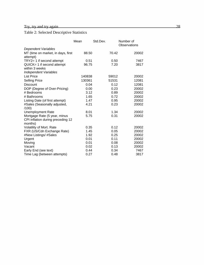
3/ Definitions of Variables

This paper studies the sequence of states shown in Table 1 plus how long a seller remains

in each state. Several types of dependent variables are considered. MT measures how long a

house was on the market on a particular attempt. If a first attempt expired, TRY2= 1 if the seller

makes a second attempt at any time after and equals 0 if no second attempt is recorded. If there

was a second attempt, QUICK= 1 if the second attempt occurred within three weeks of the end

of the first attempt and 0 otherwise.

Insert Table 2

To explain variation in these dependent variables, I consider many types of independent

variables, some6 of which are reported in Table 2. The first class of variables describe the house,

including the reported number of bedrooms and bathrooms (measured using dummy variables to

maximize the flexibility in estimation). Information on the location of each house was

constructed with the help of the GIS Lab at the University of Windsor and is based on 24 postal

code divisions. Some descriptors are coded automatically, such as the presence of a pool,

landscaping or the style of building, but several variables were constructed by scanning the

“Remarks” section of the published listing for key words, such as “Beautiful” or “Good Buy”.

Some key words revealed the intended market segment, such as “Handyman Special,” “Starter”

or “Rent”. The presence of such key words in the Remarks section is measured with dummy


7 The regression included over 60 variables and produced R2= 0.623. Individually, eachcoefficient on a variable representing an indicator of market conditions was insignificant. A tableof coefficients is available from the author.

8 Some researchers (Asabere and Huffman, 1992; Ong and Koh, 2000) have proposedusing the rate of house price inflation as an indicator. This proposal is based on the idea thatpotential capital gains could affect the decision to hold the asset. The work on informationalefficiency of a real estate market suggests that the actual rate of change probably differs from theanticipated rate. I prefer to use variables which are likely to cause prices to change. As apractical matter, this measure may vary little within the sample since the data in this study arefrom a period of fairly stable prices.

variables. In total, 29 descriptive variables were used.

The next class of variables describe the seller, including the Degree of Over-Pricing

(DOP). The method of estimating the Degree of Over-Pricing (DOP) is outlined in Anglin,

Rutherford and Springer (2003). Essentially, a buyer perceives a house as being over-priced if

its list price is high relative to the list prices of comparable houses. To implement this

comparison, I regress ln(list price) on various descriptors of a house using ordinary least squares;

the residual is DOP.7 The fact that one seller may make multiple attempts implies that the set of

houses seen by a buyer differs subtly from the set of sellers. Since DOP is intended to represent

buyers’ perception of a listing and since I assume that buyers are not fully informed about

previous attempts, I use the full data set in this regression: i.e. if a seller makes two attempts then

the house enters this regression twice. After DOP has been computed for each attempt using the

contemporaneously reported description, the entire data set is reorganized into a record of the

attempts by 20002 different sellers.

The Remarks section of the listing can reveal some information on a seller’s intentions,

such as whether the seller “Must Sell” or is moving to a new job or the house is “Vacant.” The

presence of such phrases is indicated with dummy variables. I constructed three such variables.

The next class of variables concerns market conditions. In the past, many indicators of

market conditions have been proposed in informal and formal studies. I use the following

indicators, which are available on a monthly basis.8


9 Since Windsor is a border town, a change in the exchange rate could affect the localeconomy in ways that are not measured by the unemployment rate.

Real mortgage interest rate (five year, using the inflation rate over the 12 months prior)

Volatility of real interest rate (measured as the sample standard deviation on preceding

six months)

Local unemployment rate (seasonally-adjusted)

Number of sales (seasonally-adjusted)

US/Canada exchange rate9

Balance: number of new listings/number of sales

plus seasonal variables (Winter includes the first quarter; Spring includes second quarter of each

year and so on.) Professional analysts at Canada Mortgage and Housing Corp. (CMHC) find

these measures useful but they are imperfect.

Since both market conditions and the thing being studied vary over time, I use different

measures of the same indicator in different regressions. DOP is estimated using market

conditions as they exist at the listing date. For the technical reasons described more fully below,

the selling process is estimated using the average value of each indicator over the duration of the

listing. The determinants of TRY2 and QUICK are estimated using market conditions as they

exist at the end of the first attempt.

I noted how some listings might expire before their natural end because a seller becomes

dissatisfied with the performance of their agent. But an early end may also be caused by other

forces, such as disappointment with the state of the market. The relative importance of these two

explanation should vary with the time before expiry and this fact suggests how to measure this

effect. Because of a policy imposed by the local real estate board, essentially no listings expire

during the first 60 days. Any listing which expires after exactly 61 days suggests that the seller

is most dissatisfied with the agent’s performance. For contrast, any listing which could have

expired on day 61 but actually expired after 182 days or the normal term of an agreement,

suggests that dissatisfaction with market conditions or the tastes of the seller is the dominant

Try, try and try again 16factor. To measure any effect of changing balance between these factors as the duration

increases, I let

EARLYEND= max(0, (182- MT)/(182- 60)).

Finally, TIMELAG measures the fraction of a year between the end of a first attempt and the

beginning of a second attempt.

4/ Econometric Methods and Miscellaneous Hypotheses

Practitioners and academics sense that a relationship between time and price should exist

but its magnitude, and sometimes even its sign, have been debated. The earliest papers in

refereed journals (e.g. Cubbin, 1974; Belkin, Hempel and McLeavey, 1976; Miller, 1978) used

small data sets and ordinary least squares (OLS). More recent work used two-stage least squares

(e.g. Yavas and Yang, 1995) to overcome simultaneity bias and used the discount (i.e. 1- selling

price/list price) to measure “over-pricing”. The most recent work (e.g. Glower, Haurin and

Hendershott, 1999; Anglin, Rutherford and Springer, 2003) tended to use a duration model to

study one part of the trade off more precisely and focused on the list price as a key indicator.

Given a set of explanatory variables, X, the statistical algebra uses the same principles as

a decision tree:

Probability(t# tS| first attempt, SOLD, X)= 1- S(tS; X)

where t represents the passage of time and S(.) is called the survivor function for selling. F( tS)=

1- S(tS) is the cumulative distribution function of time-till-sale. Similarly,

Probability(t# tE| first attempt, Expired, X)= 1- E(tE; X)

where E(.) is the survivor function for expiry. The distribution of time-on-the-market during the

first attempt is

MT= min(tS, tE).

As a practical matter, these two processes form a competing risk model where I estimate each

one separately as a censored process. At the end of an expired first attempt, the probability of a

second attempt is

Probability(TRY2= 1| Expired, X)= g(X)

and is estimated using a logit model. These probability functions suffice to predict the average

Try, try and try again 17probabilities shown in Table 1. I also estimate

Probability(QUICK= 1| TRY2= 1, X)= h(X)

using a logit model. The duration model proposed for the second attempt is similar to that

shown above for the first attempt.

All such studies have focused on the selling process which, according to Figure 1, is

smooth enough that the hazard function can be estimated parametrically with confidence. The

Weibull model is commonly used, in part because the Exponential distribution is a theoretically

interesting special case. In contrast, Figure 1 shows that the expiry process is not a smooth

function of duration. Instead of using a traditional parametric model, I use Cox’s proportional

hazard model (summarized by Lancaster, 1990) to estimate it.

Cox’s model starts with a baseline hazard function, h0(t), and assumes that the probability

of sale during a short period of time for a seller described by X is:

Prob(sale during (t, t+ dt); X)= h0(t) exp(X$).

Both h0(t) and $ are to be estimated. This model is a semi-parametric model in the sense that the

baseline hazard uses a step function where the size of each step is based on the data:

h0(t)= 3t "T I(t= T)

where I(t= T)= 1 if the equality is true and 0 otherwise. By construction, the probability of sale

before t is

1- S(t)= 1- exp(-It h0(T) dT exp(X$)).

When a data point is censored, these formulas are modified to account for the limited

information embodied in the observation.

This model is proportional in the sense that the ratio of the probabilities of sale for

different types of sellers at a given point in time is independent of t: given any set of houses

offered at t, G(t), the probability that seller i’s house would sell in the next short period of time is

h0(t) exp(Xi$) / (3j, G(t) h0(t) exp(Xj$))= exp(Xi$) / (3j, G(t) exp(Xj$)).

Since the right hand side of this expression is independent of the baseline hazard function, $ can

be estimated more easily. Cox’s model is also known as a “partial likelihood” method because it


10 Unobserved heterogeneity is a common problem but recent research (van den Berg,2000; Frijters, 2002) in a labor market has indicated how multiple observations of single seller,e.g. repeated attempts to sell, offer the possibility of spotting effects common to a seller acrossthe different attempts. It may be possible to detect correlations among generalized residuals(Lancaster and Chesher, 1985) that would reveal non-independent processes. This analysis isleft as future research.

11 Several explanatory variables change over time and it is theoretically possible to treatthem as “time-varying covariates.” Unfortunately, the size of the data set and technicalrestrictions in the statistical package (LIMDEP) limit my treatment of time-varying covariates. Ifocus on other questions.

does not propose a full joint likelihood function. More specifically, it cannot differentiate spells

of time when nothing in the data happens. A more serious limitation is that Cox’s model cannot

identify, and therefore ignores, unobserved heterogeneity.10 By itself, this ignorance causes

negative duration dependence where a changing selection of sellers causes the hazard rate to

appear to fall.

In practice, Figure 2 shows that the date of expiry is closely tied to dates on a calendar.

Therefore the time scale is changed to recognize the clustering of events on critical days. Instead

of using MT directly, I divide time into 24 categories. Except for a phase-in period, each month

has two periods: a period between the 3rd and 16th of each month and the period between the

17th of a month and the 2nd day of the next month. Organizing the data in this way creates a

small problem because the length of a period can varies. To reduce this effect, there is a phase-

in period, of at least one month and no more than two months long, until the beginning of the

categories described above. Because Cox’s model is a partial likelihood model, because Figure

2 shows that few listings expire between the clusters, and because Figure 1 shows that few

listings expire during the phase-in period, the qualitative effect of stretching time in this way is

small.11

5/ Results

These tables focus on the hypotheses noted above. More specifically, the regressions

include many other variables, such as the number of bedrooms or the location, that are not

reported in these tables. For the reader’s information, a large number of the individual


12 The method of estimating DOP implies that DOP is independent of market conditionsbut, even so, none of the published indicators of market conditions were significant in explainingvariation in the list price. This finding limits the validity of models which seek to explain thechoice of list price as a signal that is consistent with some equilibrium inference by buyers sinceit may be difficult to extract the signal that the seller is trying to send from the noise created bychanging external conditions.

coefficients describing the house were statistically significant in explaining the selling process

during the first attempt; fewer of these coefficients were statistically significant in explaining the

process during the second attempt, the expiry process discussed with Table 4 or the decision to

try again discussed in Table 5. In Tables 3 and 4, except for F and 2 which have particular

interpretations, a positive coefficient implies that an increase in that variable increased the

instantaneous probability of sale (decreased the expected time for that process if that process

were allowed to continue to its natural conclusion). Table 5 reports on the estimates of two logit

model and the signs of the coefficients have their usual interpretation.

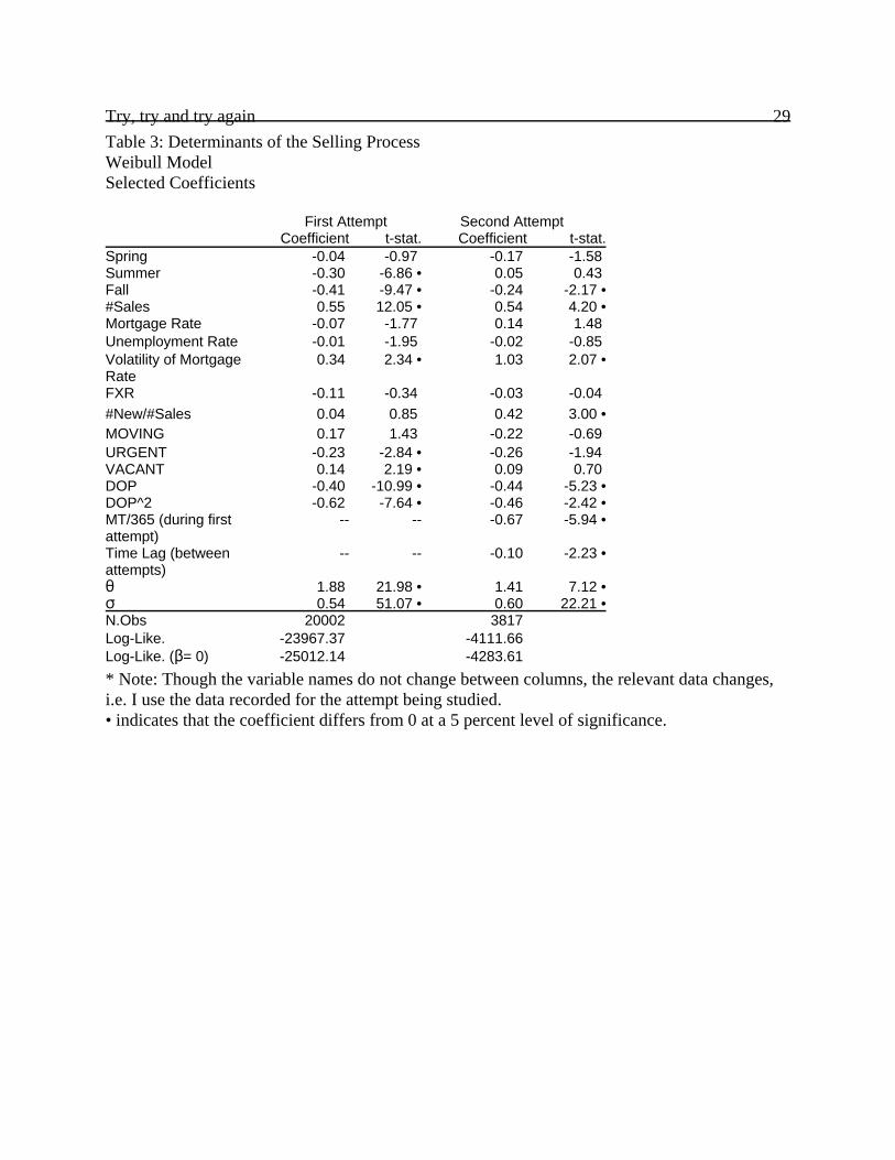
Insert Table 3

As expected, the left hand pair of columns on Table 3 show that an increase in the Degree

of Over-Pricing decreased the probability of sale at any point in time during the first attempt.

The marginal effect became more severe as DOP rose. Some of the coefficients on variables

representing market conditions and seasons were statistically significant with the probability of

sale being highest in the Winter and Spring. An increase in the unemployment rate was nearly

significant at the 5 percent level where an increase in the rate decreased the probability of sale.12

The variables measuring the seller’s motivation were significant, except for the variable showing

whether a seller intended to move in the near future, but not always with the expected sign.

F is the parameter estimated for the Weibull distribution and is significantly different

from 0 or 1; F= 0.54 implies that the baseline hazard function decreases with duration. There is

evidence of unobserved heterogeneity that can be captured by a Gamma correction. The

estimate of 2 indicates that there was significant unobserved heterogeneity amongst sellers.

Try, try and try again 20The coefficients relating to the second attempt, shown in the right hand pair of columns,

follow the same general pattern as for the first attempt except that the levels of t-statistics on the

second attempt are usually lower. The right hand columns also include two measures of the

duration before the start of the second attempt. A longer duration on an unsuccessful first

attempt decreased the instantaneous probability of sale at any point during the second attempt

and a longer time lag between attempts also decreased the probability of sale on the second

attempt. The effect of a lengthy first attempt dominated the effect of a time lag between attempts

by a factor of about 7.

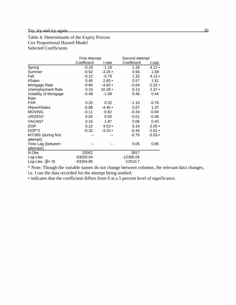
Insert Table 4

The left hand pair of columns on Table 4 report selected coefficients for the expiry

process on the first attempt using Cox’s model. For most of the range of DOP, an increase in

DOP increased the instantaneous probability that a listing would expire. For very high values of

DOP, the coefficient on DOP2 shows that this effect reaches a peak before falling. Mortgage

interest rates and unemployment rates were important determinants of the expiry process: an

decrease in the interest rate or an increase in the unemployment rate increased the probability of

expiry.

The right hand pair of columns on Table 4 report coefficients concerning the second

attempt. The seasonal pattern changed significantly but the coefficients on indicators of market

conditions were similar to those reported for the first attempt with the exception of the ratio of

new listings to sales. On the first attempt an increase in this ratio decreased the probability of

expiry whereas, on the second attempt, the coefficient was positive though insignificant.

An increase in either the duration of the first attempt decreased the probability of expiry

or an increase in the time lag between attempts decreased the probability of expiry. Again, the

effect of a prior listing dominates the effect of the intervening time by a large factor. This

finding suggests that such sellers had serious intentions during their first attempt to sell and that

the intervening time lag represents a failed attempt to sell by FSBO. This suggestion is


0.1

0.2

0.3

0.4Pe

r-per

iod

Prob

abilit

y

1 6 11 16 21Periods

First Att. Second Att.

Figure 5: Baseline Hazard Function of Expiry (per-period probability)

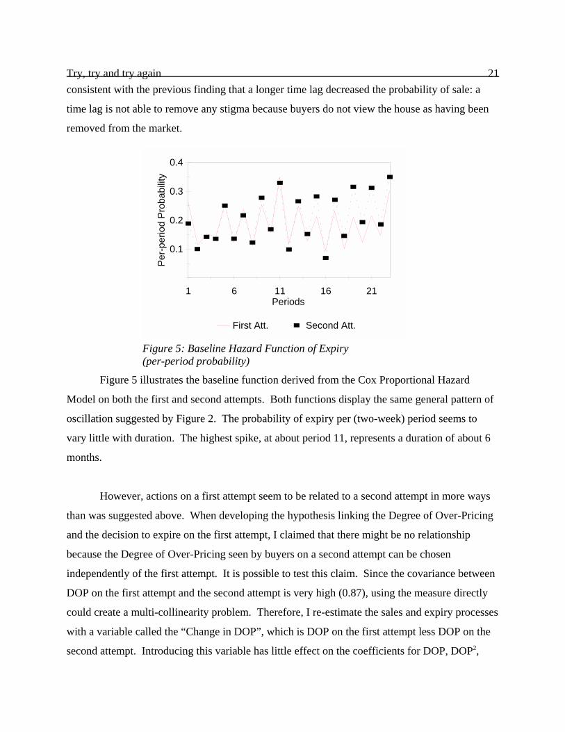
consistent with the previous finding that a longer time lag decreased the probability of sale: a

time lag is not able to remove any stigma because buyers do not view the house as having been

removed from the market.

Figure 5 illustrates the baseline function derived from the Cox Proportional Hazard

Model on both the first and second attempts. Both functions display the same general pattern of

oscillation suggested by Figure 2. The probability of expiry per (two-week) period seems to

vary little with duration. The highest spike, at about period 11, represents a duration of about 6

months.

However, actions on a first attempt seem to be related to a second attempt in more ways

than was suggested above. When developing the hypothesis linking the Degree of Over-Pricing

and the decision to expire on the first attempt, I claimed that there might be no relationship

because the Degree of Over-Pricing seen by buyers on a second attempt can be chosen

independently of the first attempt. It is possible to test this claim. Since the covariance between

DOP on the first attempt and the second attempt is very high (0.87), using the measure directly

could create a multi-collinearity problem. Therefore, I re-estimate the sales and expiry processes

with a variable called the “Change in DOP”, which is DOP on the first attempt less DOP on the

second attempt. Introducing this variable has little effect on the coefficients for DOP, DOP2,

Try, try and try again 22MT/365 or Time Lag but is negative and significant in both regressions. To be more

specifically, if I compare two second attempts having equal DOP, the attempt with the higher

DOP on the first attempt would have a lower the probability of sale and a lower probability of

expiry at any given point in time.

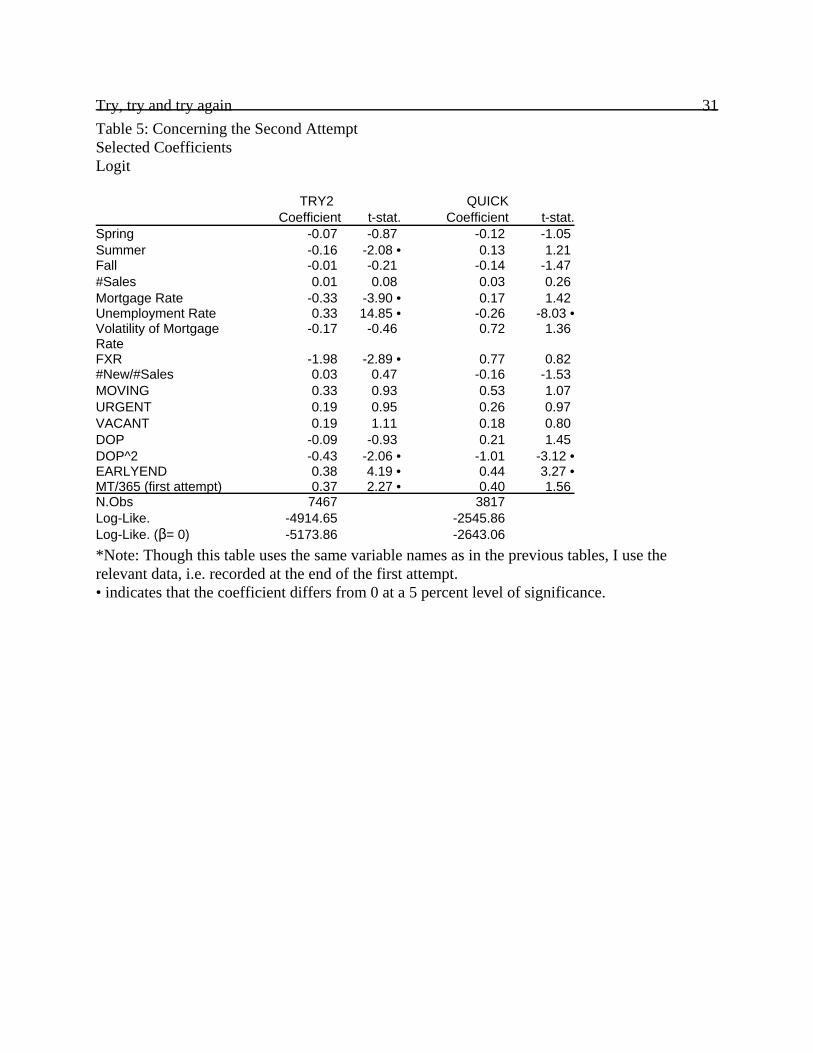
Insert Table 5

Table 5 reports selected coefficients on the decision to try again after a first attempt

failed. At the micro-level, an increase in DOP decreased the probability of a second attempt and

a seller with the highest DOP was less likely to try quickly. Sellers whose listing ended early

were more likely to try again. For those sellers who decided to make a second attempt, sellers

with a very high values of DOP on the first attempt were less likely to try again quickly and

sellers who ended another listing early were more likely to try again quickly. At the macro-

level, the mortgage interest rate and the unemployment rate had a significant effect on the

decision to try again. Surprisingly, an increase in the ratio of new sellers to sales (my proxy for

excess supply) had no significant effect on the probability or timing of a second attempt. While

some of the coefficients are statistically significant, adding the variables does little to improve

the goodness of fit.

6/ Implications

These results are mostly consistent with the hypotheses presented at the end of Section 2.

The first set of hypotheses focused on the general selling process. I found that the hazard rate,

i.e. the instantaneous probability, of sale decreased with duration and that an increase in the first

duration decreased the hazard rate for the second duration. Waiting between attempts had a

much smaller effect but with an unanticipated sign. This evidence, together with Figure 3 mostly

confirms Hypothesis 1. In part, this evidence explains why a rational seller would want to give

up an attempt rather than waiting indefinitely.

The second set of hypotheses focused on the Degree of Over-Pricing (DOP). As earlier

studies found, an increase in DOP decreased the probability of sale. I also found that an increase

Try, try and try again 23in DOP tended to increase the probability of expiry on the first attempt and to decrease the

probability of making a second attempt. Thus, Hypothesis 2 is confirmed. DOP should be seen

as a credible indicator of a seller’s bargaining position. Figure 4 suggests that the market

process tends to select the more willing sellers, i.e. those with lower values of DOP, but the

randomness inherent in the matching process removes the assurance that only the lowest priced

sellers will sell.

The fourth hypothesis focused on the role of an agent. I found some effects due to

dissatisfaction with an agent: sellers who ended a listing early were more likely to try again and

were more likely to try again quickly.

The third hypothesis focused on market conditions. I find that there are effects worthy of

future study but, since the effect of a change in market conditions is not based on any specific

theoretical model, I hesitate to attach an interpretation to any given coefficient. In an important

sense, the coefficients of the selling process and of the expiry process should be combined

because there is more than one dimension to a seller’s behavior: letting a listing expire is not

exactly the same thing as not selling. It is true that, ultimately, a house either sells or it does not

but this truth ignores the time margin. Combining results from the selling and expiry processes,

an increase in the unemployment rate decreased the probability of sale and increased the

probability that a seller would let a listing expire at any given point in time. Thomas (1996)

noted that one of the problems with using a competing risk model to explain behavior is that the

individual coefficients do not directly reveal the magnitude or sign of an effect on a selected

fraction of listings. With the coefficients estimated here and without more computations, for

example, the effect of an increase in the unemployment rate on the average time-till-sale of

houses which sell is ambiguous.

This paper ignores some practical problems with using market conditions as explanatory

variables. First, I do not distinguish between anticipated and unanticipated changes in market

conditions. Anticipated conditions, of the kind that Krainer (2001) considered, affect a seller’s

decision to enter a market and all subsequent events. Unanticipated changes may not even be

Try, try and try again 24recognized until after the seller completes the transaction with an “unanticipated” buyer. The

way that the explanatory variables are constructed has the effect of assuming that sellers are

myopic. Second, though not reported here, indicators of market conditions had little effect on

the list price. Using an independent data set covering some of the same time period as the data

used here, Anglin and Wiebe (2004) noted that the variation in DOP has a more significant effect

on the selling price than indicators of market conditions. Thus, the link between measures of

“market conditions” and the actions of individual sellers in the middle of a market is only

imperfectly understood.

It may be that the measures are too crude to be useful for the kinds of detailed

calculations that an individual seller needs to make. Or, it may be that the average price of a

house varies according to a different mechanism. Read (1988), Salant (1991), Ben-Shahar

(2003) and others have proposed models where the selling price is a function of duration. With

given conditions, this price function combines with the realized time-till-sale to produce a

realized selling price; for a given price function, a change in market conditions which changes

duration would be enough to change the average realized price. In this kind of model, it would

be vital to recognize the fact that some sellers prefer to let their listing expire rather than

continue forever.

It may be that market conditions change the selection of sellers types active in a market

but this data set cannot study this question directly because it does not include data on people

who think about selling their house. The evidence from the behavior of sellers who make a

second attempt may provide some insight, because such sellers are near the margin, but these

sellers are also selected by a process that is not fully understood.

Try, try and try again 25BibliographyAnglin, P. 1994. “A summary of some data on buying and selling houses,” working paper,University of Windsor.

Anglin, P., 2004. “The value and liquidity effects of a change in market conditions”, workingpaper, University of Windsor.

Anglin, P., R. Rutherford and T. Springer, 2003. “The trade off between the selling price andtime-on-the-market: The impact of price setting,” Journal of Real Estate Finance andEconomics, 26 (1), 95- 111.

Anglin, P. and R. Wiebe, 2002. “House prices and time-till-sale in Windsor,” report submitted tothe Windsor and Essex County Real Estate Board (with supplements).

Anglin, P., and R. Wiebe, 2004. “Pricing in an illiquid real estate market”, working paper,University of Windsor.

Asabere, P. and F. Huffman, 1992. “Macroeconomic determinants of time on the market,” RealEstate Issues, 39- 43.

Ben-Shahar, D., 2002. “Theoretical and empirical analysis of the multiperiod pricing pattern inthe real estate market,” Journal of Housing Economics, 11, 95- 107.

Canadian Real Estate Association (CREA) 2003. “Who we are” available athttp://www.crea.ca/public/about/about.htm

Capozza, D., P. Hendershott and C. Mack, 2004. “An anatomy of price dynamics in illiquidmarkets: Analysis and Evidence from local housing markets”, Real Estate Economics, 32 (1), 1-32.

Clayton, J., 1996. “Rational expectations, market fundamentals and housing price volatility,”Real Estate Economics, 24(4), 441-470.

Clayton, J., 1997. “Are housing price cycles driven by irrational expectations?,” Journal of RealEstate Finance and Economics, 14, 341-63.

Coles, M.G., and E. Smith, 1998. “Marketplaces and matching”, International EconomicReview, 39 (1), 239-54.

Dale-Johnson, D. and S. Hamilton, 1998. “Housing market conditions, listing choice and MLSmarket share,” Real Estate Economics, 26 (2), 275- 307.

Federal Trade Commission, 1983. The residential real estate brokerage industry, staff report,Los Angeles.

Try, try and try again 26Frijters, P., 2002. “The non-parametric identification of lagged duration dependence,”Economics Letters, 73 (3), 289- 292.

Forgey, F.A., R.C. Rutherford and T.M. Springer. 1996. “Search and liquidity in single-familyhousing,” Real Estate Economics, 24:3, 273-292.

Geltner, D.M., B.D. Kluger, and N. Miller, 1991. “Optimal price and selling effort from theperspectives of the broker and seller”, American Real Estate and Urban Economics AssociationJournal, 19 (1), 1- 24.

Genesove, D. and C.J. Mayer, 1997. “Equity and time to sale in the real estate market,” American Economic Review, 87:3, 255-270.

Genesove, D., and C.J. Mayer. 2001. “Loss aversion and seller behavior: Evidence from thehousing market,” Quarterly Journal of Economics

Glower, M., D.R. Haurin and P.H. Hendershott. 1998. “Selling time and selling price: Theinfluence of seller motivation,” Real Estate Economics, 26:4, 719-740.

Kalra R., and K.C. Chan, 1994. “Censored sample bias, macroeconomic factors and time onmarket of residential housing,” Journal of Real Estate Research, 9:2, 253- 262.

Keifer, N., 1988. “Economic duration data and hazard functions”, Journal of EconomicLiterature, 26, 646- 679.

Knight, J., 2002. “Listing price, time on market and ultimate selling price: Causes and effects ofhidden listing price changes,” Real Estate Economics,

Krainer, J. 2001. “A theory of liquidity in residential real estate markets,” Journal of UrbanEconomics 49, 32- 53.

Lambson, V., G. McQueen and B. Slade, 2003. “Do out-of-state buyers pay more? Anexamination of anchoring induced bias and search costs”, Real Estate Economics, 32 (1), 85-126.

Lancaster, T., 1990. The econometric analysis of transition data, Cambridge University Press,New York.

Lancaster, T. and A. Chesher, 1985. “Residual analysis for censored duration data,” EconomicsLetters, 18, 35- 38.

Lin, Z. and K. Vandell, 2001. “Illiquidity and real estate risk,” working paper, University ofWisconsin- Madison School of Business.

Miceli, T., 1989. “The optimal duration of real estate listing contracts”, American Real Estate

Try, try and try again 27and Urban Economics Association Journal, 17(3), 267-77. Mortensen, International Economic Review

Novy- Marx, R., 2002. “The fine line between hot and cold markets”, working paper, HaasSchool of Business, University of California, Berkeley.

Ong, S.E., and Y.C. Koh, 2000. “Time-on-market and price trade-offs in high-rise housingsub-markets”, Urban Studies, 37 (11), 2057-71.

Ortalo-Magne, F., and A. Merlo, 2002. “Bargaining over real estate: Evidence from England,working paper,” University of Wisconsin.

Pissarides, C., 2000. Equilibrium unemployment theory, MIT Press, Cambridge, MA.

Read, C., 1988. “Price strategies for idiosyncratic goods- The case of housing,” American RealEstate and Urban Economics Association Journal, 16(4), 379- 395.

Rosen, S., 1974. “Hedonic prices and implicit markets,” Journal of Political Economy, 82 (1),34- 55.

Salant, S., 1991. “For sale by owner: When to use a broker and how to price the house,” Journalof Real Estate Finance and Economics, 4 (2), 157- 173.

Stein, J.C., 1995. “Prices and trading volume in the housing market: a model with down-paymenteffects,” Quarterly Journal of Economics, 110:2, 379-406.

Taylor, C., 1999. “Time-on-the-market as a sign of quality,” Review of Economic Studies, 66 (3),555-78.

Thomas, J. 1996. “On the interpretation of covariate estimates in independent competing risksmodels,” Bulletin of Economic Research, 48 (1), 27- 39.

Yavas, A. 1992. “A simple search and bargaining model of real estate markets,” Journal of theAmerican Real Estate and Urban Economics Association (now Real Estate Economics), 20:4,533-548.

Yavas, A. and S. Yang, 1995. “The strategic role of listing price in marketing real estate: Theoryand evidence,” Real Estate Economics, 23 (3), 347- 368.

van den Berg, G., 2000. “Duration models: Specification, Identification and MultipleDurations,” working paper, Free University Amsterdam; forthcoming chapter in Handbook ofEconometrics, Vol. V ed. by J. Heckman and E. Leamer.

Zorn, T., and W.H. Sackley, 1991. “Buyers’ and sellers’ markets: A simple rational expectationssearch model of the housing market,” Journal of Real Estate Finance and Economics, 4 (3).

Try, try and try again 28Table 2: Selected Descriptive Statistics

Mean Std.Dev. Number ofObservations

Dependent Variables MT (time on market, in days, firstattempt)

88.50 70.42 20002

TRY2= 1 if second attempt 0.51 0.50 7467 QUICK= 1 if second attemptwithin 3 weeks

96.75 7.20 3817

Independent VariablesList Price 140838 59012 20002 Selling Price 130361 51531 12081 Discount 0.04 0.12 12081 DOP (Degree of Over-Pricing) 0.00 0.23 20002 # Bedrooms 3.12 0.89 20002 # Bathrooms 1.65 0.72 20002 Listing Date (of first attempt) 1.47 0.95 20002 #Sales (Seasonally adjusted,/100)

4.21 0.23 20002

Unemployment Rate 8.01 1.34 20002 Mortgage Rate (5 year, minusCPI inflation during preceding 12months)

5.75 0.31 20002

Volatility of Mort. Rate 0.35 0.12 20002 FXR (US/Cdn Exchange Rate) 1.45 0.05 20002 #New Listings/ #Sales 1.92 0.25 20002 Urgent 0.01 0.11 20002 Moving 0.01 0.08 20002 Vacant 0.02 0.13 20002 Early End (see text) 0.44 0.34 7467 Time Lag (between attempts) 0.27 0.48 3817

Try, try and try again 29Table 3: Determinants of the Selling Process Weibull Model Selected Coefficients

First Attempt Second Attempt Coefficient t-stat. Coefficient t-stat.

Spring -0.04 -0.97 -0.17 -1.58 Summer -0.30 -6.86 • 0.05 0.43 Fall -0.41 -9.47 • -0.24 -2.17 •#Sales 0.55 12.05 • 0.54 4.20 •Mortgage Rate -0.07 -1.77 0.14 1.48 Unemployment Rate -0.01 -1.95 -0.02 -0.85 Volatility of MortgageRate

0.34 2.34 • 1.03 2.07 •

FXR -0.11 -0.34 -0.03 -0.04 #New/#Sales 0.04 0.85 0.42 3.00 •MOVING 0.17 1.43 -0.22 -0.69 URGENT -0.23 -2.84 • -0.26 -1.94 VACANT 0.14 2.19 • 0.09 0.70 DOP -0.40 -10.99 • -0.44 -5.23 •DOP^2 -0.62 -7.64 • -0.46 -2.42 •MT/365 (during firstattempt)

-- -- -0.67 -5.94 •

Time Lag (betweenattempts)

-- -- -0.10 -2.23 •

2 1.88 21.98 • 1.41 7.12 •F 0.54 51.07 • 0.60 22.21 •N.Obs 20002 3817 Log-Like. -23967.37 -4111.66 Log-Like. ($= 0) -25012.14 -4283.61 * Note: Though the variable names do not change between columns, the relevant data changes,i.e. I use the data recorded for the attempt being studied. • indicates that the coefficient differs from 0 at a 5 percent level of significance.

Try, try and try again 30Table 4: Determinants of the Expiry Process Cox Proportional Hazard Model Selected Coefficients

First Attempt Second Attempt Coefficient t-stat. Coefficient t-stat.

Spring -0.18 -1.19 1.26 4.12 •Summer -0.52 -3.26 • 0.56 1.58 Fall -0.12 -0.79 1.32 4.13 •#Sales 0.40 2.83 • 0.57 1.91 Mortgage Rate -0.66 -4.60 • -0.64 -2.32 •Unemployment Rate 0.16 10.28 • 0.13 2.37 •Volatility of MortgageRate

-0.48 -1.08 0.46 0.44

FXR 0.20 0.32 -1.16 -0.76 #New/#Sales -0.88 -4.46 • 0.57 1.37 MOVING -0.11 -0.62 -0.34 -0.94 URGENT 0.05 0.50 -0.01 -0.06 VACANT 0.16 1.87 0.06 0.43 DOP 0.22 4.53 • 0.19 2.00 •DOP^2 -0.32 -3.15 • -0.44 -2.01 •MT/365 (during firstattempt)

-- -- -0.75 -5.03 •

Time Lag (betweenattempts)

-- -- 0.05 0.85

N.Obs 20002 3817 Log-Like. -63020.54 -12365.05 Log-Like. ($= 0) -63264.85 -12510.7 * Note: Though the variable names do not change between columns, the relevant data changes,i.e. I use the data recorded for the attempt being studied. • indicates that the coefficient differs from 0 at a 5 percent level of significance.

Try, try and try again 31Table 5: Concerning the Second Attempt Selected Coefficients Logit

TRY2 QUICKCoefficient t-stat. Coefficient t-stat.

Spring -0.07 -0.87 -0.12 -1.05 Summer -0.16 -2.08 • 0.13 1.21 Fall -0.01 -0.21 -0.14 -1.47 #Sales 0.01 0.08 0.03 0.26 Mortgage Rate -0.33 -3.90 • 0.17 1.42 Unemployment Rate 0.33 14.85 • -0.26 -8.03 •Volatility of MortgageRate

-0.17 -0.46 0.72 1.36

FXR -1.98 -2.89 • 0.77 0.82 #New/#Sales 0.03 0.47 -0.16 -1.53 MOVING 0.33 0.93 0.53 1.07 URGENT 0.19 0.95 0.26 0.97 VACANT 0.19 1.11 0.18 0.80 DOP -0.09 -0.93 0.21 1.45 DOP^2 -0.43 -2.06 • -1.01 -3.12 •EARLYEND 0.38 4.19 • 0.44 3.27 •MT/365 (first attempt) 0.37 2.27 • 0.40 1.56 N.Obs 7467 3817 Log-Like. -4914.65 -2545.86 Log-Like. ($= 0) -5173.86 -2643.06 *Note: Though this table uses the same variable names as in the previous tables, I use therelevant data, i.e. recorded at the end of the first attempt. • indicates that the coefficient differs from 0 at a 5 percent level of significance.