


Languages
Pages
Legal

The Role of International Public Goods in Tax
Cooperation
Pantelis Kammas* and Apostolis Philippopoulosy
Abstract
We provide a quantitative assessment of the welfare cost of tax competition or, equiva-
lently, the welfare benefit of international tax policy cooperation. We use a simple multi-
country general equilibrium model of a world economy, in which there are two types of
cross-country spillovers: the first one generated by the international capital mobility and,
the second one, by the presence of international public goods. In the absence of interna-
tional public goods, although welfare in the non-cooperative case is typically lower than in
the cooperative case, the welfare difference is negligible quantitatively. Things change
drastically, both quantitatively and qualitatively, once we introduce international public
goods. Now, there can be big benefits from cooperation and welfare effects cease to be
monotonic. (JEL classification codes: F02, H2, H4)
Keywords: Capital mobility, tax competition, public goods, welfare
1 Introduction
One of the main results in international economics is that non-cooperative
(Nash) national tax policies lead to a race-to-the-bottom and suboptimal
outcomes. Hence, there is need for international cooperation. Such argu-
ments become stronger as the degree of economic integration increases
and tax competition becomes fiercer.1
* Department of Economics, University of Ioannina. e-mail: [email protected] Department of Economics, Athens University of Economics and Business, Department of
Economics, University of Glasgow and CESifo. e-mail: [email protected] are grateful to the editor and two anonymous referees for constructive criticisms andsuggestions. We thank K. Angelopoulos, G. Economides, C. Kotsogiannis and H. Parkfor discussions and comments. We have also benefited from comments by A. Adam,M. Delis, V. Dioikitopoulos, T. Moutos and N. Tsakiris. Any errors are ours. Thefirst co-author acknowledges financial support from the Greek Ministry of Educationand the European Union under the ‘Iraklitos’ research fellowship programme.
1 See, for example, Persson and Tabellini (1992, 1995), who also reviewed the literature.The standard race-to-the-bottom result is usually derived in a setup where the onlycross-country spillover effect, or externality, is generated by international capital mobilityand where national policy instruments are chosen by Ramsey (benevolent) policymakers.A similar setup is used here. Note that international cooperation can becomecounter-productive if we depart from Ramsey policymakers, and there are failures atpolicymaking level. Here we do not study such issues, so cooperation is superior tonon-cooperation. See Razin and Sadka (1999) for various political–economy aspects oftax competition. For empirical evidence of tax competition in OECD countries, see, forexample, Devereux, Lockwood and Redoano (2008).
� The Author 2009. Published by Oxford University Presson behalf of Ifo Institute for Economic Research, Munich. All rights reserved.For permissions, please email: [email protected] 278
CESifo Economic Studies, Vol. 56, 2/2010, 278–299 doi:10.1093/cesifo/ifp025Advance Access publication 9 November 2009
at Athens U
niversity of Econom
ics and Business on M
ay 13, 2011cesifo.oxfordjournals.org
Dow
nloaded from

But recent quantitative studies using general equilibrium models withRamsey-type policymakers indicate that the welfare gains from coordi-nated tax policies are not significant quantitatively (see, e.g., Mendozaand Tezar, 2005 and Sørensen, 2004). In most of these studies, the welfaregains from coordination are around 1 percent of gross domestic productand remain robustly ‘small’ across different model specifications andpolicy scenarios.2
In this article, we re-examine the quantitative welfare implication ofinternational tax cooperation. The difference from most of the relatedliterature is that we incorporate an international public good, namely apublic good, whose benefits can extend beyond national boundaries (seealso Bjorvatn and Schjelderup, 2002). As Tabellini (2003) pointed out,such goods constitute an important factor of the European Union (EU).Examples include foreign or defence policy and environmental quality.In addition, the abolition of borders between EU member states has gen-erated a status of increased cross-country spillovers in several areas suchas internal security, immigration policy and scientific research. We showthat the incorporation of international public goods in a model of inter-national tax competition changes the above-mentioned results drastically.We use a multi-country version of the general equilibrium model in
Persson and Tabellini (1992). This is a simple and tractable model.There are two types of cross-border spillovers. The first one is generatedby international capital mobility and results in the problem of tax com-petition for mobile tax bases. The second spillover is generated by thepresence of international public goods and results in the problem of freeriding on other countries’ contribution.When we solve the model numerically to get a measure of general equi-
librium welfare, our results are as follows. In the absence of internationalpublic goods, the welfare gain from cooperation is quantitatively small.The reason is that higher tax rates (as we switch from Nash to coopera-tion) is good for public goods provision in the short run, but they are badfor private investment and, in turn, future consumption. The latter offsetsthe beneficial effect of higher public goods provision in the short run.Thus, in a non-static setup, suboptimally low Nash tax rates are notthat bad quantitatively, as already shown by, for example, Mendozaand Tezar (2005).Results change drastically once we introduce international public goods.
Although, as mentioned above, we realize that what is small or large is
2 What is ‘small’ or ‘large’ is of course arbitrary. One percent gain may be considered to belarge enough. The key point, however, is whether the welfare gain from cooperationchanges substantially across different model specifications. Here we show that it does,once we introduce international public goods.
CESifo Economic Studies, 56, 2/2010 279
The Role of International Public Goods in Tax Cooperation
at Athens U
niversity of Econom
ics and Business on M
ay 13, 2011cesifo.oxfordjournals.org
Dow
nloaded from
arbitrary and we should be cautious how to read these numbers, it is fair
and robust to claim that (a) the introduction of international public goods
into a rather conventional model with international capital mobility makes
the welfare gain from cooperation particularly big. Thus, the argument for
international cooperation becomes much stronger when there are public
goods that extend beyond national borders. (b) The combination of the
two spillovers has qualitative implications too. The welfare gain from
cooperation is nonmonotonic in the magnitude of cross-country spilloversfrom international public goods; after a turning point, the welfare gain
falls with this magnitude (see also Bjorvatn and Schjelderup, 2002, for
similar effects on tax rates).The rest of the article is as follows. Section 2 solves for a world com-
petitive equilibrium (WCE). Section 3 solves for optimal policies. Section 4
concludes.
2 World economy
Consider a world economy composed of a finite number of identical
countries N, indexed by i ¼ 1,2, . . . ,N. Each country i is populated by a
representative private agent and a benevolent Ramsey national govern-
ment. The private agent in each country consumes and invests at home
and abroad, where investment abroad implies a mobility or transaction
cost (the latter provides a measure of the degree of capital mobility). The
national government in each country taxes domestic and foreign investorsat the same rate (source principle of taxation) to finance the provision of a
public good whose benefits can extend beyond national boundaries.We use a simple two-period (present and future) model adapted from
Persson and Tabellini (1992). The differences are that here we use a multi-
country version of this model and add an international public good as in
Bjorvatn and Schjelderup (2002). All countries produce the same com-
modity and have access to a linear technology.The sequence of events is as follows. In the beginning of the game,
national governments choose once-and-for-all their tax policies and the
associated contributions to the public good. In turn, private agents max-
imize their lifetime utility making their investment and (present and
future) consumption decisions. Working with backward induction, wefirst solve the private agents’ problem by taking prices and policies as
given. This will give us a WCE, which is for any feasible tax policies. In
turn, we solve for Nash national tax policies. Namely, each national gov-
ernment chooses its own tax rate optimally subject to the WCE by taking
as given the tax policies of the other government. We also solve for coop-
erative national policies; this will serve as a benchmark.
280 CESifo Economic Studies, 56, 2/2010
P. Kammas and A. Philippopoulos
at Athens U
niversity of Econom
ics and Business on M
ay 13, 2011cesifo.oxfordjournals.org
Dow
nloaded from
2.1 Behaviour of private agents
The representative household in each country i maximizes
Ui ¼ Uðci1,ci2,G
iÞ ð1aÞ
where ci1 and ci2 are private consumption in the first and second period,
respectively, and Gi is the international public good from the viewpoint of
private agent located in country i (see equation (5) below). The utility
function is increasing and quasi-concave. For algebraic simplicity, we
use an additively separable function of the form
Ui ¼ log ci1 þ ci2 þ �Gi ð1bÞ
where � is the weight given to public services relative to private
consumption.3
The first-period budget constraint of the private agent in country i is
ci1 þ kii þXN
jð6¼iÞ¼1
kij ¼ ei ð2aÞ
that is, the private agent begins with an exogenous endowment, ei, and
uses this endowment for consumption, ci1, investment at home, kii, and
investment in other countries j 6¼ i denoted as kij.The second-period budget constraint of the private agent in country i is
ci2 ¼ ð1� tiÞAikii þXN
jð6¼iÞ¼1
ð1� tjÞAjkij �XN
jð6¼iÞ¼1
mijðkijÞ2
2ð2bÞ
where 0 < ti < 1 and 0 < tj < 1 are income tax rates in countries i and
j 6¼ i, respectively, the parameters Ai > 0 and Aj > 0 are the exogenous
capital returns in i and j, respectively, and mij � 0 is a measure of mobility
costs when an investor located in i invests in j 6¼ i (as said above, mij
3 Persson and Tabellini (1992) also use a utility function that is linear in second-periodoutcomes (but they abstract from utility-enhancing public goods). In the numerical solu-tions presented in Section 3 below, in order to get a well-defined general equilibriumsolution, we need a relatively high value of the valuation of public services (�), whentax policies are chosen non-cooperatively (Nash). Intuitively, tax competition leads to toolow tax rates and too small provision of public services (Gi) relative to private consump-tion (ci2), so that one needs to value public services a lot to restore their desirability. Inparticular, one needs to value them more than concurrent private consumption (hence,� > 1). This is not required when tax policies are chosen cooperatively (in that case, wecan get a solution even if � < 1). Also note that, even in the Nash case, one can set lowervalues of � (although always in the range � > 1), when the degree of cross-country spil-lovers from international public goods (see b in equation (5) below) rises; this is because band � are substitutes with optimally chosen policies. See Section 3 below for furtherdetails.
CESifo Economic Studies, 56, 2/2010 281
The Role of International Public Goods in Tax Cooperation
at Athens U
niversity of Econom
ics and Business on M
ay 13, 2011cesifo.oxfordjournals.org
Dow
nloaded from
provides a measure of international capital mobility, where mij ¼ 0 implies
perfect mobility and mij!1 zero mobility).4
Private agents act competitively by taking policy variables as given.
Substituting equations (2a) and (2b) into (1b), the first-order conditions
with respect to kii and kij give, respectively (these are Euler-type equations)
1
ci1¼ ð1� tiÞAi ð3aÞ
1
ci1¼ ð1� tjÞAj �mijkij for j 6¼ i ð3bÞ
so that ð1� tiÞAi ¼ ð1� tjÞAj �mijkij. Thus, without uncertainty, net
returns are equalized.
2.2 National government budget constraint
Each national government i spends gi on a public good by taxing domestic
and foreign investors at the same rate, 0 < ti < 1. Thus, assuming a
balanced budget, the budget constraint of national government in
country i is
gi ¼ tiAiki ð4Þ
where ki ¼ kii þ�Njð6¼iÞ¼1k
ji denotes the total capital stock in country i (kji is
the capital invested in country i by investors located in country j 6¼ i).
2.3 International public good
To model the international public good Gi, as defined in equations (1a)
and (1b) above, we follow, for example, Alesina and Wacziarg (1999) and
Bjorvatn and Schjelderup (2002), by assuming
Gi ¼ gi þ bXN
jð6¼iÞ¼1
gj ð5Þ
where the parameter 0 � b � 1 measures the strength of international spil-
lovers in public good provision. When b ¼ 0, there is no spillover and the
public good is national or local. When b ¼ 1, there are perfect spillovers
and the public good is fully international.
4 Strictly speaking, since these costs materialize in the second period, while investment takesplace in the first period, these costs are costs of repatriation rather than costs of investingabroad. But, since this is not important algebraically, we prefer to use the terminology ofPersson and Tabellini (1992).
282 CESifo Economic Studies, 56, 2/2010
P. Kammas and A. Philippopoulos
at Athens U
niversity of Econom
ics and Business on M
ay 13, 2011cesifo.oxfordjournals.org
Dow
nloaded from
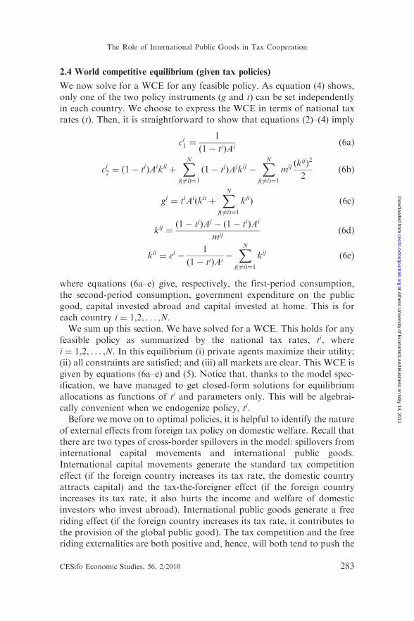
2.4 World competitive equilibrium (given tax policies)
We now solve for a WCE for any feasible policy. As equation (4) shows,only one of the two policy instruments (g and t) can be set independentlyin each country. We choose to express the WCE in terms of national taxrates (t). Then, it is straightforward to show that equations (2)–(4) imply
ci1 ¼1
ð1� tiÞAið6aÞ
ci2 ¼ ð1� tiÞAikii þXN
jð6¼iÞ¼1
ð1� tjÞAjkij �XN
jð6¼iÞ¼1
mij ðkijÞ
2
2ð6bÞ
gi ¼ tiAiðkii þXN
jð6¼iÞ¼1
kjiÞ ð6cÞ
kij ¼ð1� tjÞAj � ð1� tiÞAi
mijð6dÞ
kii ¼ ei �1
ð1� tiÞAi�
XNjð6¼iÞ¼1
kij ð6eÞ
where equations (6a–e) give, respectively, the first-period consumption,the second-period consumption, government expenditure on the publicgood, capital invested abroad and capital invested at home. This is foreach country i ¼ 1,2, . . . ,N.We sum up this section. We have solved for a WCE. This holds for any
feasible policy as summarized by the national tax rates, ti, wherei ¼ 1,2, . . . ,N. In this equilibrium (i) private agents maximize their utility;(ii) all constraints are satisfied; and (iii) all markets are clear. This WCE isgiven by equations (6a–e) and (5). Notice that, thanks to the model spec-ification, we have managed to get closed-form solutions for equilibriumallocations as functions of ti and parameters only. This will be algebrai-cally convenient when we endogenize policy, ti.Before we move on to optimal policies, it is helpful to identify the nature
of external effects from foreign tax policy on domestic welfare. Recall thatthere are two types of cross-border spillovers in the model: spillovers frominternational capital movements and international public goods.International capital movements generate the standard tax competitioneffect (if the foreign country increases its tax rate, the domestic countryattracts capital) and the tax-the-foreigner effect (if the foreign countryincreases its tax rate, it also hurts the income and welfare of domesticinvestors who invest abroad). International public goods generate a freeriding effect (if the foreign country increases its tax rate, it contributes tothe provision of the global public good). The tax competition and the freeriding externalities are both positive and, hence, will both tend to push the
CESifo Economic Studies, 56, 2/2010 283
The Role of International Public Goods in Tax Cooperation
at Athens U
niversity of Econom
ics and Business on M
ay 13, 2011cesifo.oxfordjournals.org
Dow
nloaded from
uncoordinated tax rate below its Pareto efficient value. The tax-the-
foreigner effect can be negative or positive depending on whether the
domestic country is exporter or importer of capital and, hence, can
work in either direction.5 We let the solution below to determine the net
final externality and, hence, how Nash and cooperative policies may differ.
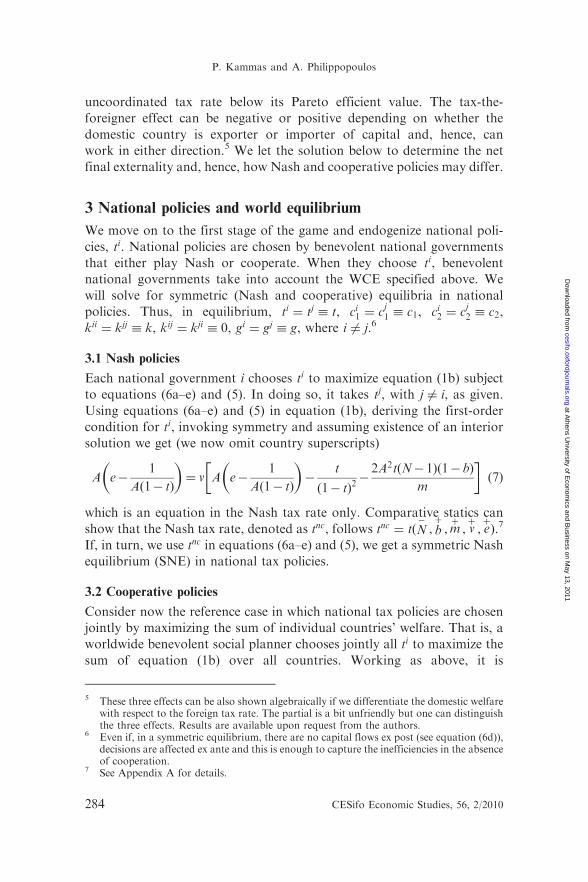
3 National policies and world equilibrium
We move on to the first stage of the game and endogenize national poli-
cies, ti. National policies are chosen by benevolent national governments
that either play Nash or cooperate. When they choose ti, benevolent
national governments take into account the WCE specified above. We
will solve for symmetric (Nash and cooperative) equilibria in national
policies. Thus, in equilibrium, ti ¼ tj � t, ci1 ¼ cj1 � c1, ci2 ¼ cj2 � c2,
kii ¼ kjj � k, kij ¼ kji � 0, gi ¼ gj � g, where i 6¼ j.6
3.1 Nash policies
Each national government i chooses ti to maximize equation (1b) subject
to equations (6a–e) and (5). In doing so, it takes tj, with j 6¼ i, as given.
Using equations (6a–e) and (5) in equation (1b), deriving the first-order
condition for ti, invoking symmetry and assuming existence of an interior
solution we get (we now omit country superscripts)
A e�1
Að1� tÞ
� �¼ v A e�
1
Að1� tÞ
� ��
t
ð1� tÞ2�2A2tðN� 1Þð1� bÞ
m
� �ð7Þ
which is an equation in the Nash tax rate only. Comparative statics can
show that the Nash tax rate, denoted as tnc, follows tnc ¼ tðN�
, bþ
,mþ, vþ, eþÞ.7
If, in turn, we use tnc in equations (6a–e) and (5), we get a symmetric Nash
equilibrium (SNE) in national tax policies.
3.2 Cooperative policies
Consider now the reference case in which national tax policies are chosen
jointly by maximizing the sum of individual countries’ welfare. That is, a
worldwide benevolent social planner chooses jointly all ti to maximize the
sum of equation (1b) over all countries. Working as above, it is
5 These three effects can be also shown algebraically if we differentiate the domestic welfarewith respect to the foreign tax rate. The partial is a bit unfriendly but one can distinguishthe three effects. Results are available upon request from the authors.
6 Even if, in a symmetric equilibrium, there are no capital flows ex post (see equation (6d)),decisions are affected ex ante and this is enough to capture the inefficiencies in the absenceof cooperation.
7 See Appendix A for details.
284 CESifo Economic Studies, 56, 2/2010
P. Kammas and A. Philippopoulos
at Athens U
niversity of Econom
ics and Business on M
ay 13, 2011cesifo.oxfordjournals.org
Dow
nloaded from
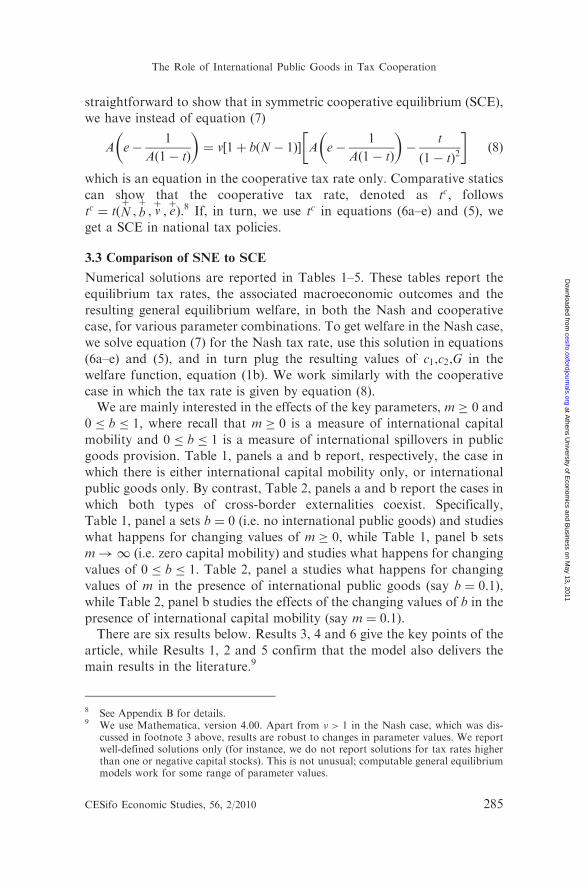
straightforward to show that in symmetric cooperative equilibrium (SCE),
we have instead of equation (7)
A e�1
Að1� tÞ
� �¼ v½1þ bðN� 1Þ� A e�
1
Að1� tÞ
� ��
t
ð1� tÞ2
� �ð8Þ
which is an equation in the cooperative tax rate only. Comparative statics
can show that the cooperative tax rate, denoted as tc, follows
tc ¼ tðNþ
, bþ
, vþ, eþÞ.8 If, in turn, we use tc in equations (6a–e) and (5), we
get a SCE in national tax policies.
3.3 Comparison of SNE to SCE
Numerical solutions are reported in Tables 1–5. These tables report the
equilibrium tax rates, the associated macroeconomic outcomes and the
resulting general equilibrium welfare, in both the Nash and cooperative
case, for various parameter combinations. To get welfare in the Nash case,
we solve equation (7) for the Nash tax rate, use this solution in equations
(6a–e) and (5), and in turn plug the resulting values of c1,c2,G in the
welfare function, equation (1b). We work similarly with the cooperative
case in which the tax rate is given by equation (8).We are mainly interested in the effects of the key parameters, m � 0 and
0 � b � 1, where recall that m � 0 is a measure of international capital
mobility and 0 � b � 1 is a measure of international spillovers in public
goods provision. Table 1, panels a and b report, respectively, the case in
which there is either international capital mobility only, or international
public goods only. By contrast, Table 2, panels a and b report the cases in
which both types of cross-border externalities coexist. Specifically,
Table 1, panel a sets b ¼ 0 (i.e. no international public goods) and studies
what happens for changing values of m � 0, while Table 1, panel b sets
m!1 (i.e. zero capital mobility) and studies what happens for changing
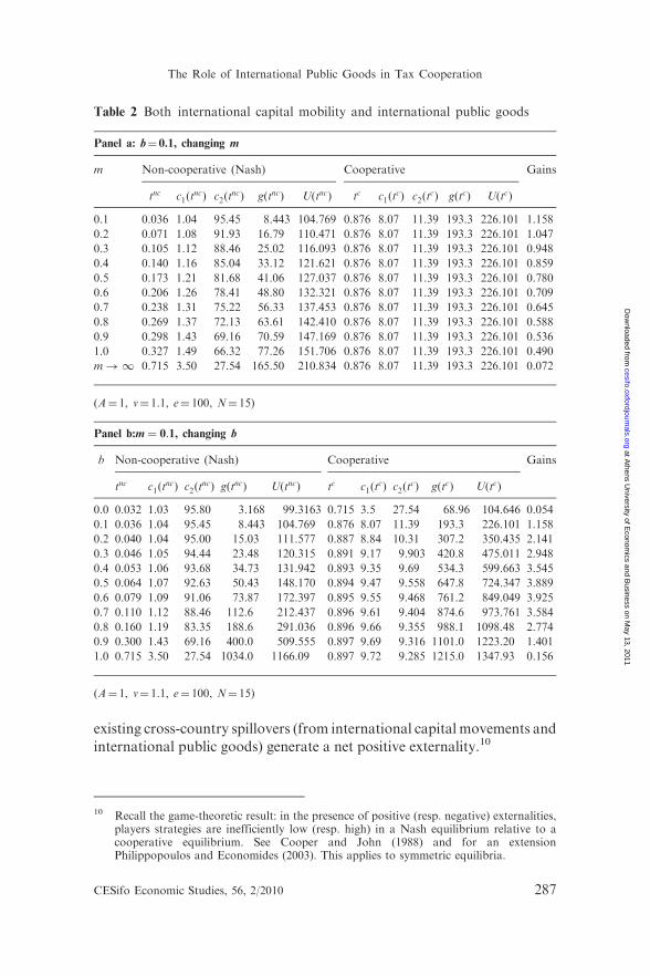
values of 0 � b � 1. Table 2, panel a studies what happens for changing
values of m in the presence of international public goods (say b ¼ 0:1),while Table 2, panel b studies the effects of the changing values of b in the
presence of international capital mobility (say m ¼ 0:1).There are six results below. Results 3, 4 and 6 give the key points of the
article, while Results 1, 2 and 5 confirm that the model also delivers the
main results in the literature.9
8 See Appendix B for details.9 We use Mathematica, version 4.00. Apart from � > 1 in the Nash case, which was dis-
cussed in footnote 3 above, results are robust to changes in parameter values. We reportwell-defined solutions only (for instance, we do not report solutions for tax rates higherthan one or negative capital stocks). This is not unusual; computable general equilibriummodels work for some range of parameter values.
CESifo Economic Studies, 56, 2/2010 285
The Role of International Public Goods in Tax Cooperation
at Athens U
niversity of Econom
ics and Business on M
ay 13, 2011cesifo.oxfordjournals.org
Dow
nloaded from

Result 1. In all cases, the Nash tax rate is less than, or equal to, the coop-
erative tax rate (i.e. 0 < tnc � tc < 1). Also, welfare under Nash is less
than, or equal to, welfare under cooperation. Only when we set m!1
and b ¼ 0 in Table 1, panel a (i.e. neither international capital mobility, nor
international public goods, so that the economies are practically closed),
the two solutions coincide. In all ‘interior’ cases (0 � m <1 and/or b > 0),
the Nash tax rate is found to be suboptimally low. This means that the
Table 1 Either international capital mobility or international public goods only
Panel a: b¼ 0, changing m
m Non-cooperative (Nash) Cooperative Gains
tnc c1ðtncÞ c2ðt
ncÞ gðtncÞ UðtncÞ tc c1ðtcÞ c2ðt
cÞ gðtcÞ UðtcÞ
0.1 0.032 1.03 95.8 3.168 99.3163 0.715 3.5 27.54 68.96 104.646 0.054
0.2 0.064 1.07 92.63 6.304 99.6282 0.715 3.5 27.54 68.96 104.646 0.050
0.3 0.095 1.11 89.49 9.403 99.9352 0.715 3.5 27.54 68.96 104.646 0.047
0.4 0.126 1.14 86.40 12.46 100.236 0.715 3.5 27.54 68.96 104.646 0.044
0.5 0.156 1.19 83.35 15.46 100.531 0.715 3.5 27.54 68.96 104.646 0.041
0.6 0.186 1.23 80.36 18.41 100.818 0.715 3.5 27.54 68.96 104.646 0.038
0.7 0.216 1.27 77.44 21.29 101.097 0.715 3.5 27.54 68.96 104.646 0.035
0.8 0.244 1.32 74.59 24.09 101.366 0.715 3.5 27.54 68.96 104.646 0.032
0.9 0.272 1.37 71.83 26.80 101.624 0.715 3.5 27.54 68.96 104.646 0.030
1.0 0.298 1.43 69.16 29.41 101.871 0.715 3.5 27.54 68.96 104.646 0.027
m!1 0.715 3.50 27.54 68.96 104.646 0.715 3.5 27.54 68.96 104.646 0.000
(A¼ 1, v¼ 1.1, e¼ 100, N¼ 15)
Panel b: m!1, changing b
b Non-cooperative (Nash) Cooperative Gains
tnc c1ðtncÞ c2ðt
ncÞ gðtncÞ UðtncÞ tc c1ðtcÞ c2ðt
cÞ gðtcÞ UðtcÞ
0.0 0.715 3.50 27.54 68.95 104.646 0.715 3.5 27.54 68.96 104.646 0.000
0.1 0.715 3.50 27.54 165.5 210.834 0.876 8.07 11.39 193.3 226.101 0.072
0.2 0.715 3.50 27.54 262.0 317.022 0.887 8.84 10.31 307.2 350.435 0.105
0.3 0.715 3.50 27.54 358.6 423.211 0.891 9.17 9.903 420.8 475.011 0.122
0.4 0.715 3.50 27.54 455.1 529.402 0.893 9.35 9.690 534.3 599.663 0.133
0.5 0.715 3.50 27.54 551.6 635.593 0.894 9.47 9.558 647.8 724.347 0.140
0.6 0.715 3.50 27.54 648.2 741.785 0.895 9.55 9.468 761.2 849.049 0.145
0.7 0.715 3.50 27.54 744.7 847.978 0.896 9.61 9.404 874.6 973.761 0.148
0.8 0.715 3.50 27.54 841.3 954.175 0.896 9.66 9.355 988.1 1098.48 0.151
0.9 0.715 3.50 27.54 937.8 1060.39 0.897 9.69 9.316 1101.0 1223.20 0.154
1.0 0.715 3.50 27.54 1034.0 1166.09 0.897 9.72 9.285 1215.0 1347.93 0.156
(A¼ 1, v¼ 1.1, N¼ 15, e¼ 100)
286 CESifo Economic Studies, 56, 2/2010
P. Kammas and A. Philippopoulos
at Athens U
niversity of Econom
ics and Business on M
ay 13, 2011cesifo.oxfordjournals.org
Dow
nloaded from
existing cross-country spillovers (from international capital movements and
international public goods) generate a net positive externality.10
Table 2 Both international capital mobility and international public goods
Panel a: b¼ 0.1, changing m
m Non-cooperative (Nash) Cooperative Gains
tnc c1ðtncÞ c2ðt
ncÞ gðtncÞ UðtncÞ tc c1ðtcÞ c2ðt
cÞ gðtcÞ UðtcÞ
0.1 0.036 1.04 95.45 8.443 104.769 0.876 8.07 11.39 193.3 226.101 1.158
0.2 0.071 1.08 91.93 16.79 110.471 0.876 8.07 11.39 193.3 226.101 1.047
0.3 0.105 1.12 88.46 25.02 116.093 0.876 8.07 11.39 193.3 226.101 0.948
0.4 0.140 1.16 85.04 33.12 121.621 0.876 8.07 11.39 193.3 226.101 0.859
0.5 0.173 1.21 81.68 41.06 127.037 0.876 8.07 11.39 193.3 226.101 0.780
0.6 0.206 1.26 78.41 48.80 132.321 0.876 8.07 11.39 193.3 226.101 0.709
0.7 0.238 1.31 75.22 56.33 137.453 0.876 8.07 11.39 193.3 226.101 0.645
0.8 0.269 1.37 72.13 63.61 142.410 0.876 8.07 11.39 193.3 226.101 0.588
0.9 0.298 1.43 69.16 70.59 147.169 0.876 8.07 11.39 193.3 226.101 0.536
1.0 0.327 1.49 66.32 77.26 151.706 0.876 8.07 11.39 193.3 226.101 0.490
m!1 0.715 3.50 27.54 165.50 210.834 0.876 8.07 11.39 193.3 226.101 0.072
(A¼ 1, v¼ 1.1, e¼ 100, N¼ 15)
Panel b:m ¼ 0:1, changing b
b Non-cooperative (Nash) Cooperative Gains
tnc c1ðtncÞ c2ðt
ncÞ gðtncÞ UðtncÞ tc c1ðtcÞ c2ðt
cÞ gðtcÞ UðtcÞ
0.0 0.032 1.03 95.80 3.168 99.3163 0.715 3.5 27.54 68.96 104.646 0.054
0.1 0.036 1.04 95.45 8.443 104.769 0.876 8.07 11.39 193.3 226.101 1.158
0.2 0.040 1.04 95.00 15.03 111.577 0.887 8.84 10.31 307.2 350.435 2.141
0.3 0.046 1.05 94.44 23.48 120.315 0.891 9.17 9.903 420.8 475.011 2.948
0.4 0.053 1.06 93.68 34.73 131.942 0.893 9.35 9.69 534.3 599.663 3.545
0.5 0.064 1.07 92.63 50.43 148.170 0.894 9.47 9.558 647.8 724.347 3.889
0.6 0.079 1.09 91.06 73.87 172.397 0.895 9.55 9.468 761.2 849.049 3.925
0.7 0.110 1.12 88.46 112.6 212.437 0.896 9.61 9.404 874.6 973.761 3.584
0.8 0.160 1.19 83.35 188.6 291.036 0.896 9.66 9.355 988.1 1098.48 2.774
0.9 0.300 1.43 69.16 400.0 509.555 0.897 9.69 9.316 1101.0 1223.20 1.401
1.0 0.715 3.50 27.54 1034.0 1166.09 0.897 9.72 9.285 1215.0 1347.93 0.156
(A¼ 1, v¼ 1.1, e¼ 100, N¼ 15)
10 Recall the game-theoretic result: in the presence of positive (resp. negative) externalities,players strategies are inefficiently low (resp. high) in a Nash equilibrium relative to acooperative equilibrium. See Cooper and John (1988) and for an extensionPhilippopoulos and Economides (2003). This applies to symmetric equilibria.
CESifo Economic Studies, 56, 2/2010 287
The Role of International Public Goods in Tax Cooperation
at Athens U
niversity of Econom
ics and Business on M
ay 13, 2011cesifo.oxfordjournals.org
Dow
nloaded from
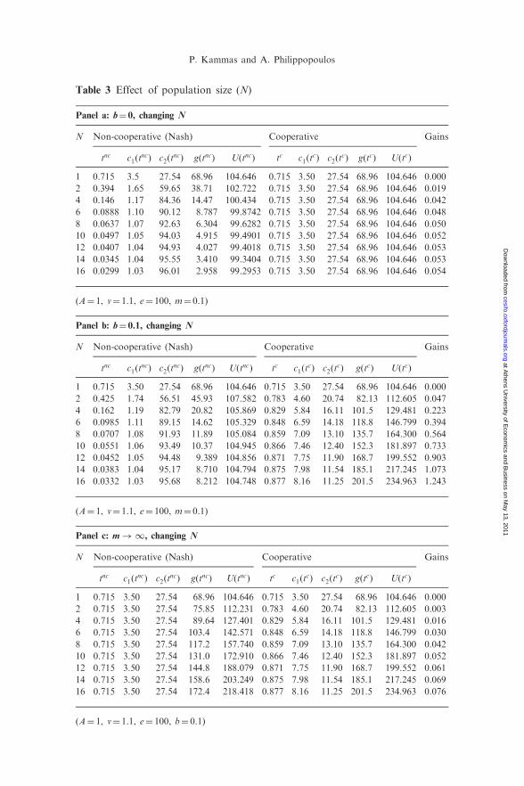
Table 3 Effect of population size (N)
Panel a: b¼ 0, changing N
N Non-cooperative (Nash) Cooperative Gains
tnc c1ðtncÞ c2ðt
ncÞ gðtncÞ UðtncÞ tc c1ðtcÞ c2ðt
cÞ gðtcÞ UðtcÞ
1 0.715 3.5 27.54 68.96 104.646 0.715 3.50 27.54 68.96 104.646 0.000
2 0.394 1.65 59.65 38.71 102.722 0.715 3.50 27.54 68.96 104.646 0.019
4 0.146 1.17 84.36 14.47 100.434 0.715 3.50 27.54 68.96 104.646 0.042
6 0.0888 1.10 90.12 8.787 99.8742 0.715 3.50 27.54 68.96 104.646 0.048
8 0.0637 1.07 92.63 6.304 99.6282 0.715 3.50 27.54 68.96 104.646 0.050
10 0.0497 1.05 94.03 4.915 99.4901 0.715 3.50 27.54 68.96 104.646 0.052
12 0.0407 1.04 94.93 4.027 99.4018 0.715 3.50 27.54 68.96 104.646 0.053
14 0.0345 1.04 95.55 3.410 99.3404 0.715 3.50 27.54 68.96 104.646 0.053
16 0.0299 1.03 96.01 2.958 99.2953 0.715 3.50 27.54 68.96 104.646 0.054
(A¼ 1, v¼ 1.1, e¼ 100, m¼ 0.1)
Panel b: b¼ 0.1, changing N
N Non-cooperative (Nash) Cooperative Gains
tnc c1ðtncÞ c2ðt
ncÞ gðtncÞ UðtncÞ tc c1ðtcÞ c2ðt
cÞ gðtcÞ UðtcÞ
1 0.715 3.50 27.54 68.96 104.646 0.715 3.50 27.54 68.96 104.646 0.000
2 0.425 1.74 56.51 45.93 107.582 0.783 4.60 20.74 82.13 112.605 0.047
4 0.162 1.19 82.79 20.82 105.869 0.829 5.84 16.11 101.5 129.481 0.223
6 0.0985 1.11 89.15 14.62 105.329 0.848 6.59 14.18 118.8 146.799 0.394
8 0.0707 1.08 91.93 11.89 105.084 0.859 7.09 13.10 135.7 164.300 0.564
10 0.0551 1.06 93.49 10.37 104.945 0.866 7.46 12.40 152.3 181.897 0.733
12 0.0452 1.05 94.48 9.389 104.856 0.871 7.75 11.90 168.7 199.552 0.903
14 0.0383 1.04 95.17 8.710 104.794 0.875 7.98 11.54 185.1 217.245 1.073
16 0.0332 1.03 95.68 8.212 104.748 0.877 8.16 11.25 201.5 234.963 1.243
(A¼ 1, v¼ 1.1, e¼ 100, m¼ 0.1)
Panel c: m!1, changing N
N Non-cooperative (Nash) Cooperative Gains
tnc c1ðtncÞ c2ðt
ncÞ gðtncÞ UðtncÞ tc c1ðtcÞ c2ðt
cÞ gðtcÞ UðtcÞ
1 0.715 3.50 27.54 68.96 104.646 0.715 3.50 27.54 68.96 104.646 0.000
2 0.715 3.50 27.54 75.85 112.231 0.783 4.60 20.74 82.13 112.605 0.003
4 0.715 3.50 27.54 89.64 127.401 0.829 5.84 16.11 101.5 129.481 0.016
6 0.715 3.50 27.54 103.4 142.571 0.848 6.59 14.18 118.8 146.799 0.030
8 0.715 3.50 27.54 117.2 157.740 0.859 7.09 13.10 135.7 164.300 0.042
10 0.715 3.50 27.54 131.0 172.910 0.866 7.46 12.40 152.3 181.897 0.052
12 0.715 3.50 27.54 144.8 188.079 0.871 7.75 11.90 168.7 199.552 0.061
14 0.715 3.50 27.54 158.6 203.249 0.875 7.98 11.54 185.1 217.245 0.069
16 0.715 3.50 27.54 172.4 218.418 0.877 8.16 11.25 201.5 234.963 0.076
(A¼ 1, v¼ 1.1, e¼ 100, b¼ 0.1)
P. Kammas and A. Philippopoulos
at Athens U
niversity of Econom
ics and Business on M
ay 13, 2011cesifo.oxfordjournals.org
Dow
nloaded from
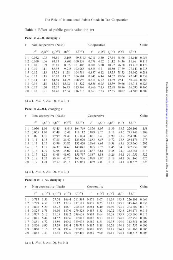
Table 4 Effect of public goods valuation (v)
Panel a: b¼ 0, changing v
v Non-cooperative (Nash) Cooperative Gains
tnc c1ðtncÞ c2ðt
ncÞ gðtncÞ UðtncÞ tc c1ðtcÞ c2ðt
cÞ gðtcÞ UðtcÞ
1.1 0.032 1.03 95.80 3.168 99.3163 0.715 3.50 27.54 68.96 104.646 0.0541.2 0.059 1.06 93.13 5.803 100.159 0.779 4.52 21.12 74.36 111.86 0.1171.3 0.081 1.09 90.88 8.029 101.405 0.808 5.20 18.22 76.58 119.419 0.1781.4 0.10 1.11 88.95 9.935 102.968 0.825 5.71 16.50 77.79 127.143 0.2351.5 0.12 1.13 87.28 11.58 104.784 0.837 6.12 15.35 78.53 134.962 0.2881.6 0.13 1.15 85.82 13.02 106.804 0.845 6.44 14.52 79.04 142.842 0.3371.7 0.14 1.17 84.54 14.29 108.993 0.851 6.72 13.89 79.4 150.764 0.3831.8 0.16 1.18 83.39 15.42 111.322 0.856 6.95 13.39 79.66 158.718 0.4261.9 0.17 1.20 82.37 16.43 113.769 0.860 7.15 12.98 79.86 166.695 0.4652.0 0.18 1.21 81.45 17.34 116.316 0.863 7.33 12.65 80.02 174.689 0.502
(A¼ 1, N¼ 15, e¼ 100, m¼ 0.1)
Panel b: b¼ 0.1, changing v
v Non-cooperative (Nash) Cooperative Gains
tnc c1ðtncÞ c2ðt
ncÞ gðtncÞ UðtncÞ tc c1ðtcÞ c2ðt
cÞ gðtcÞ UðtcÞ
1.1 0.036 1.04 95.45 8.443 104.769 0.876 8.07 11.39 193.3 226.101 1.1581.2 0.065 1.07 92.49 15.47 111.112 0.879 8.25 11.11 193.5 245.442 1.2081.3 0.09 1.10 89.99 21.40 117.894 0.881 8.40 10.90 193.7 264.802 1.2461.4 0.11 1.13 87.85 26.47 125.020 0.883 8.53 10.72 193.8 284.176 1.2731.5 0.13 1.15 85.99 30.86 132.420 0.884 8.64 10.58 193.9 303.560 1.2921.6 0.15 1.17 84.37 34.69 140.041 0.885 8.73 10.45 194.0 322.952 1.3061.7 0.16 1.19 82.95 38.07 147.844 0.887 8.81 10.35 194.0 342.351 1.3161.8 0.17 1.21 81.68 41.07 155.797 0.887 8.88 10.26 194.1 361.755 1.3221.9 0.18 1.23 80.54 43.75 163.876 0.888 8.95 10.18 194.1 381.163 1.3262.0 0.19 1.24 79.52 46.16 172.063 0.889 9.00 10.11 194.1 400.575 1.328
(A¼ 1, N¼ 15, e¼ 100, m¼ 0.1)
Panel c: m!1, changing v
v Non-cooperative (Nash) Cooperative Gains
tnc c1ðtncÞ c2ðt
ncÞ gðtncÞ UðtncÞ tc c1ðtcÞ c2ðt
cÞ gðtcÞ UðtcÞ
1.1 0.715 3.50 27.54 166.4 211.393 0.876 8.07 11.39 193.3 226.101 0.0691.2 0.779 4.52 21.12 179.5 237.517 0.879 8.25 11.11 193.5 245.442 0.0331.3 0.808 5.20 18.22 186.1 260.545 0.881 8.40 10.90 193.7 264.802 0.0161.4 0.825 5.71 16.50 187.0 279.828 0.883 8.53 10.72 193.8 284.176 0.0151.5 0.837 6.12 15.35 188.2 299.658 0.884 8.64 10.58 193.9 303.560 0.0131.6 0.845 6.44 14.52 189.6 319.813 0.885 8.73 10.45 194.0 322.952 0.0091.7 0.851 6.72 13.89 190.8 339.936 0.887 8.81 10.35 194.0 342.351 0.0071.8 0.856 6.95 13.39 191.4 359.719 0.887 8.88 10.26 194.1 361.755 0.0061.9 0.860 7.15 12.98 191.6 379.056 0.888 8.95 10.18 194.1 381.163 0.0052.0 0.863 7.33 12.65 192.6 399.400 0.889 9.00 10.11 194.1 400.575 0.003
(A¼ 1, N¼ 15, e¼ 100, b¼ 0.1)
The Role of International Public Goods in Tax Cooperation
at Athens U
niversity of Econom
ics and Business on M
ay 13, 2011cesifo.oxfordjournals.org
Dow
nloaded from
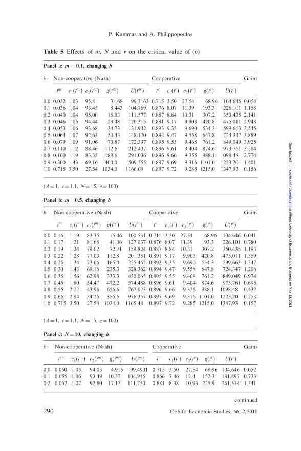
Table 5 Effects of m, N and v on the critical value of (b)
Panel a: m ¼ 0:1, changing b
b Non-cooperative (Nash) Cooperative Gains
tnc c1ðtncÞ c2ðt
ncÞ gðtncÞ UðtncÞ tc c1ðtcÞ c2ðt
cÞ gðtcÞ UðtcÞ
0.0 0.032 1.03 95.8 3.168 99.3163 0.715 3.50 27.54 68.96 104.646 0.054
0.1 0.036 1.04 95.45 8.443 104.769 0.876 8.07 11.39 193.3 226.101 1.158
0.2 0.040 1.04 95.00 15.03 111.577 0.887 8.84 10.31 307.2 350.435 2.141
0.3 0.046 1.05 94.44 23.48 120.315 0.891 9.17 9.903 420.8 475.011 2.948
0.4 0.053 1.06 93.68 34.73 131.942 0.893 9.35 9.690 534.3 599.663 3.545
0.5 0.064 1.07 92.63 50.43 148.170 0.894 9.47 9.558 647.8 724.347 3.889
0.6 0.079 1.09 91.06 73.87 172.397 0.895 9.55 9.468 761.2 849.049 3.925
0.7 0.110 1.12 88.46 112.6 212.437 0.896 9.61 9.404 874.6 973.761 3.584
0.8 0.160 1.19 83.35 188.6 291.036 0.896 9.66 9.355 988.1 1098.48 2.774
0.9 0.300 1.43 69.16 400.0 509.555 0.897 9.69 9.316 1101.0 1223.20 1.401
1.0 0.715 3.50 27.54 1034.0 1166.09 0.897 9.72 9.285 1215.0 1347.93 0.156
(A¼ 1, v¼ 1.1, N¼ 15, e¼ 100)
Panel b: m¼ 0.5, changing b
b Non-cooperative (Nash) Cooperative Gains
tnc c1ðtncÞ c2ðt
ncÞ gðtncÞ UðtncÞ tc c1ðtcÞ c2ðt
cÞ gðtcÞ UðtcÞ
0.0 0.16 1.19 83.35 15.46 100.531 0.715 3.50 27.54 68.96 104.646 0.041
0.1 0.17 1.21 81.68 41.06 127.037 0.876 8.07 11.39 193.3 226.101 0.780
0.2 0.19 1.24 79.62 72.71 159.824 0.887 8.84 10.31 307.2 350.435 1.193
0.3 0.22 1.28 77.03 112.8 201.351 0.891 9.17 9.903 420.8 475.011 1.359
0.4 0.25 1.34 73.66 165.0 255.462 0.893 9.35 9.690 534.3 599.663 1.347
0.5 0.30 1.43 69.16 235.3 328.362 0.894 9.47 9.558 647.8 724.347 1.206
0.6 0.36 1.56 62.98 333.3 430.065 0.895 9.55 9.468 761.2 849.049 0.974
0.7 0.45 1.80 54.47 472.2 574.488 0.896 9.61 9.404 874.6 973.761 0.695
0.8 0.55 2.22 43.96 656.6 767.023 0.896 9.66 9.355 988.1 1098.48 0.432
0.9 0.65 2.84 34.26 855.5 976.357 0.897 9.69 9.316 1101.0 1223.20 0.253
1.0 0.715 3.50 27.54 1034.0 1165.48 0.897 9.72 9.285 1215.0 1347.93 0.157
(A¼ 1, v¼ 1.1, N¼ 15, e¼ 100)
Panel c: N¼ 10, changing b
b Non-cooperative (Nash) Cooperative Gains
tnc c1ðtncÞ c2ðt
ncÞ gðtncÞ UðtncÞ tc c1ðtcÞ c2ðt
cÞ gðtcÞ UðtcÞ
0.0 0.050 1.05 94.03 4.915 99.4901 0.715 3.50 27.54 68.96 104.646 0.052
0.1 0.055 1.06 93.49 10.37 104.945 0.866 7.46 12.4 152.3 181.897 0.733
0.2 0.062 1.07 92.80 17.17 111.750 0.881 8.38 10.93 225.9 261.574 1.341
continued
290 CESifo Economic Studies, 56, 2/2010
P. Kammas and A. Philippopoulos
at Athens U
niversity of Econom
ics and Business on M
ay 13, 2011cesifo.oxfordjournals.org
Dow
nloaded from

Table 5 Continued
b Non-cooperative (Nash) Cooperative Gains
tnc c1ðtncÞ c2ðt
ncÞ gðtncÞ UðtncÞ tc c1ðtcÞ c2ðt
cÞ gðtcÞ UðtcÞ
0.3 0.071 1.08 91.93 25.89 120.476 0.886 8.81 10.35 299.1 341.542 1.835
0.4 0.082 1.09 90.76 37.47 132.067 0.89 9.06 10.04 372.1 421.608 2.192
0.5 0.099 1.11 89.15 53.6 148.206 0.892 9.22 9.847 445.1 501.718 2.385
0.6 0.120 1.14 86.74 77.58 172.204 0.893 9.33 9.714 518.1 581.853 2.379
0.7 0.160 1.19 82.79 116.9 211.557 0.894 9.42 9.617 591.0 662.002 2.129
0.8 0.240 1.31 75.22 192.5 287.203 0.895 9.48 9.543 664.0 742.160 1.584
0.9 0.420 1.74 56.51 379.9 474.990 0.895 9.54 9.485 736.9 822.326 0.731
1.0 0.715 3.50 27.54 689.6 786.640 0.896 9.58 9.438 809.8 902.496 0.147
(A¼ 1, v¼ 1.1, m¼ 0.1, e¼ 100)
Panel d: N¼ 20, changing b
b Non-cooperative (Nash) Cooperative Gains
tnc c1ðtncÞ c2ðt
ncÞ gðtncÞ UðtncÞ tc c1ðtcÞ c2ðt
cÞ gðtcÞ UðtcÞ
0.0 0.024 1.02 96.64 2.337 99.2334 0.715 3.50 27.54 68.96 104.646 0.055
0.1 0.026 1.03 96.38 7.528 104.685 0.882 8.44 10.84 234.1 270.452 1.583
0.2 0.029 1.03 96.05 14.01 111.493 0.89 9.10 9.991 388.4 439.407 2.941
0.3 0.034 1.03 95.63 22.34 120.236 0.893 9.36 9.678 542.4 608.568 4.061
0.4 0.039 1.04 95.07 33.42 131.876 0.895 9.51 9.516 696.4 777.789 4.898
0.5 0.047 1.05 94.29 48.91 148.139 0.896 9.60 9.416 850.3 947.036 5.393
0.6 0.059 1.06 93.13 72.06 172.453 0.897 9.66 9.349 1004 1116.30 5.473
0.7 0.078 1.08 91.19 110.4 212.752 0.897 9.71 9.300 1158 1285.57 5.043
0.8 0.120 1.13 87.37 186.3 292.402 0.897 9.74 9.263 1312 1454.84 3.975
0.9 0.230 1.29 76.38 404.1 521.183 0.898 9.77 9.235 1466 1624.12 2.116
1.0 0.715 3.50 27.54 1379.2 1545.20 0.898 9.79 9.212 1620 1793.40 0.161
(A¼ 1, v¼ 1.1, m¼ 0.1, e¼ 100)
Panel e: v¼ 1.2, changing b
b Non-cooperative (Nash) Cooperative Gains
tnc c1ðtncÞ c2ðt
ncÞ gðtncÞ UðtncÞ tc c1ðtcÞ c2ðt
cÞ gðtcÞ UðtcÞ
0.0 0.059 1.06 93.13 5.803 100.159 0.779 4.52 21.12 74.36 111.86 0.117
0.1 0.065 1.07 92.49 15.47 111.112 0.879 8.25 11.11 193.5 245.442 1.209
0.2 0.073 1.08 91.68 27.52 124.783 0.888 8.95 10.18 307.3 381.163 2.055
0.3 0.084 1.09 90.64 43.00 142.324 0.892 9.24 9.818 420.9 517.096 2.633
0.4 0.097 1.11 89.26 63.57 165.646 0.894 9.41 9.626 534.4 653.096 2.943
0.5 0.12 1.13 87.34 92.25 198.160 0.895 9.52 9.507 647.8 789.125 2.982
0.6 0.15 1.17 84.47 135.00 246.600 0.896 9.59 9.427 761.2 925.171 2.752
continued
CESifo Economic Studies, 56, 2/2010 291
The Role of International Public Goods in Tax Cooperation
at Athens U
niversity of Econom
ics and Business on M
ay 13, 2011cesifo.oxfordjournals.org
Dow
nloaded from

In what follows (i.e. Results 2–6 below), we investigate the implicationsof introducing international public goods. As we show, the interplaybetween international public goods and international capital flows haveimportant implications for the welfare gains from cooperation, both quan-titatively and qualitatively.Result 2. It is useful to start with quantitative results in the popular
special case in which there are no international public goods. This is thecase in Table 1, panel a. In the absence of international public goods(b ¼ 0), the welfare difference between the Nash case and the cooperativecase is relatively small. This happens even when the tax rates differ a lotbetween the two cases. For instance, when the mobility cost is m ¼ 1, theNash tax rate is tnc ¼ 0:298, while the socially optimal tax rate istc ¼ 0:715. Nevertheless, despite this big difference in tax rates, the utilitylevels are pretty close: UðtncÞ ¼ 101:871 in the Nash case versus
Table 5 Continued
b Non-cooperative (Nash) Cooperative Gains
tnc c1ðtncÞ c2ðt
ncÞ gðtncÞ UðtncÞ tc c1ðtcÞ c2ðt
cÞ gðtcÞ UðtcÞ
0.7 0.19 1.24 79.76 205.30 326.287 0.896 9.65 9.368 874.7 1061.23 2.252
0.8 0.28 1.40 70.64 341.20 480.365 0.897 9.69 9.323 988.1 1197.29 1.492
0.9 0.51 2.03 48.19 677.00 861.302 0.897 9.72 9.289 1101 1333.35 0.548
1.0 0.779 4.52 21.12 1115.40 1360.26 0.897 9.75 9.261 1215 1469.42 0.080
A¼ 1, N¼ 15, m¼ 0.1, e¼ 100)
Panel f: v¼ 1.5, changing b
b Non-cooperative (Nash) Cooperative Gains
tnc c1ðtncÞ c2ðt
ncÞ gðtncÞ UðtncÞ tc c1ðtcÞ c2ðt
cÞ gðtcÞ UðtcÞ
0.0 0.12 1.13 87.28 11.58 104.784 0.837 6.12 15.35 78.53 134.962 0.288
0.1 0.13 1.15 85.99 30.86 132.42 0.884 8.64 10.58 193.9 303.56 1.292
0.2 0.15 1.17 84.38 54.89 166.883 0.891 9.17 9.907 307.5 473.393 1.837
0.3 0.17 1.20 82.32 85.7 211.046 0.894 9.40 9.637 421.0 643.38 2.049
0.4 0.19 1.24 79.58 126.6 269.642 0.895 9.53 9.491 534.4 813.418 2.017
0.5 0.23 1.30 75.78 183.3 351.035 0.896 9.62 9.399 647.9 983.479 1.802
0.6 0.29 1.41 70.16 267.2 471.37 0.897 9.67 9.337 761.3 1153.55 1.447
0.7 0.38 1.61 61.12 402.5 665.307 0.897 9.72 9.291 874.7 1323.63 0.990
0.8 0.54 2.16 45.25 641.6 1008.37 0.897 9.75 9.256 988.1 1493.72 0.481
0.9 0.74 3.89 24.71 971.0 1482.60 0.898 9.78 9.229 1102.0 1663.80 0.122
1.0 0.837 6.12 15.35 1177.95 1783.062 0.898 9.80 9.207 1215.0 1833.89 0.029
(A¼ 1, N¼ 15, m¼ 0.1, e¼ 100)
292 CESifo Economic Studies, 56, 2/2010
P. Kammas and A. Philippopoulos
at Athens U
niversity of Econom
ics and Business on M
ay 13, 2011cesifo.oxfordjournals.org
Dow
nloaded from

UðtcÞ ¼ 104:646 in the cooperative case, so that the welfare gains fromcoordination are 2.7 percentage points.The intuition behind this result is revealed by looking at macroeconomic
outcomes. Recall that utility depends on both private consumption andpublic good provision (see equation (1b)). Our numerical simulationsimply that higher tax rates (as we switch from Nash to cooperation) canbe good for public good provision, but are particularly bad for second-period private consumption. This happens because higher tax rates hurtprivate investment and in turn future private consumption (see equation(6b)) so that the beneficial effect of higher tax rates gets smaller.Therefore, in a dynamic setup, Nash tax rates are not that bad quantita-tively. This is different from a static model, where higher tax rates canincrease the provision of public goods without hurting the economy in thefuture. The standard argument—that tax competition is harmful in thepresence of cross-country spillovers—becomes weaker in a dynamic setup.Finally, in Table 1, panel a, the effect of m is monotonic, in the sense
that as capital mobility rises and tax competition gets fiercer (i.e. as m getssmaller), the difference between the two (Nash and cooperative) tax ratesand, hence, the gain from cooperation rises. This monotonic effect alsoholds in the presence of international public goods (see Table 2, panel abelow), that is, it holds for any value of 0 � b � 1.Result 3. Consider now the symmetrically opposite case from the one
described above. Namely, there is zero capital mobility (m!1) so that itis only public goods that generate cross-border spillovers. This case isreported in Table 1, panel b. The benefits from cooperation becomebigger than those in Table 1, panel a. Thus, free riding problems mattermore than problems associated with internationally mobile tax bases.Also note that, in the absence of capital mobility, the welfare benefit is
monotonic in b (see Table 1, panel b). That is, without capital mobility, asthe magnitude of international spillovers from public goods provisionincreases, the incentive to free ride on other countries’ provision ofpublic goods becomes stronger, and, hence, the difference between thetwo (Nash and cooperative) tax rates and the gain from cooperationrise monotonically.Result 4. Now, in Table 2, panels a and b, both spillovers are present.
The combination of international capital mobility (0 � m <1) and inter-national public goods (b > 0) makes the gains for cooperation really big.For instance, compare Table 1, panel a (zero international spillover frompublic goods) to Table 2, panel a (a modest degree of international spil-lover from public goods) by focusing on the same magnitude of interna-tional capital mobility; when say m ¼ 1, the welfare gain from cooperationis 49 percentage points in Table 2, panel a, while it was only 2.7 percentagepoints in Table 1, panel a. The fact that it is the combination of the two
CESifo Economic Studies, 56, 2/2010 293
The Role of International Public Goods in Tax Cooperation
at Athens U
niversity of Econom
ics and Business on M
ay 13, 2011cesifo.oxfordjournals.org
Dow
nloaded from

spillovers that makes the quantitative difference is confirmed when wecompare Table 1, panel b (no capital mobility) and Table 2, panel b (cap-ital mobility), both for varying values of 0 � b � 1. The benefits are muchbigger in Table 2, panel b. Thus, the introduction of international publicgoods into a model with international capital mobility has drastic quan-titative welfare implications.It is also important to note that, for given 0 � m <1, the effect of b is
not monotonic. This is shown in Table 2, panel b, where we set saym ¼ 0:1 and examine the effects from changes in 0 � b � 1. Up to a crit-ical value of b, denoted as b�, which is around 0.6 in Table 2, panel b, thehigher the magnitude of international spillovers from public goods provi-sion, or the worse the free riding problem, the higher the welfare gain fromcooperation. But after b�, the higher is the value of b, the lower getsthe welfare gain from cooperation. This happens because, after b�, asthe public good turns from local to international, the incentive to competefor mobile tax bases is reduced. Actually, in the special case of full inter-national spillovers from provided public goods (b ¼ 1), the incentive tocompete for mobile tax bases, and the distortions associated with this, arecompletely eliminated. This is shown by the fact that when b ¼ 1, thesolution is independent of the value of m (see, e.g., Table 1, panel b andTable 2, panel b). This is similar to the main result in Bjorvatn andSchjelderup (2002, proposition 1).11 Nevertheless, as also pointed out byBjorvatn and Schjelderup, there is still undersupply of public goods in theNash equilibrium due to free riding. Summarizing, when both interna-tional spillovers are present, they do not simply add up to a single extern-ality; their interaction is nonlinear in the sense that the effects of b arenonmonotonic.12
Result 5. We next report the effects of other parameter values. Table 3,panels a–c report results for changing values of population size (N), when,respectively, there is capital mobility but no international public goods(0 � m <1 and b ¼ 0), there are both capital mobility and internationalpublic goods (0 � m <1 and b > 0) and there are international publicgoods but no capital mobility (b > 0 and m!1). Results are monotonic.The welfare gain from cooperation increases with the size of population.This happens because, in symmetric equilibria, coordination problems, orNash-type inefficiencies, get worse with the number of players.13
11 Bjorvatn and Schjelderup (2002, Section 3) also review the earlier literatures on mobiletax bases and spillovers in public goods provision, and discuss how this result (i.e. theelimination of the tax competition effect in the presence of full spillovers from publicgoods) is related to those literatures. Differences between our work and that in Bjorvatnand Schjelderup are clarified in Section 4 below.
12 We are grateful to a referee for pointing this out to us.13 In the case of asymmetric equilibria, the relation is ambiguous.
294 CESifo Economic Studies, 56, 2/2010
P. Kammas and A. Philippopoulos
at Athens U
niversity of Econom
ics and Business on M
ay 13, 2011cesifo.oxfordjournals.org
Dow
nloaded from
Table 4, panels a–c report what happens when the valuation of the
public good (�) changes. We consider the same three cases as above.
Results are again monotonic. In Table 4, panels a–b, with capital mobility,as � rises, the welfare gain from cooperation gets larger. By contrast, in
Table 4, panel c, without capital mobility, as � rises, the welfare gain from
cooperation gets smaller. The idea in Table 4, panel c is that, when the
only international spillover is from public goods provision, the more we
value public goods, the more we internalize cross-country spillovers even
in the absence of cooperation. On the other hand, when there is alsointernational capital mobility, as in Table 4, panels a–b, the dominant
effect of � is through international capital flows.Result 6. Combining the above results, it is only the value of 0 � b � 1
that produces humped-shaped effects on the gain from cooperation, and
this happens when both international public goods and international cap-ital mobility are present. Results are summarized in Table 5, panels a–b
(two different values of mobility costs), 5c–d (two different values of pop-
ulation size) and 5e–f (two different values of public goods valuation). In
all these tables, both spillovers are present and we experiment with chan-
ging values of 0 � b � 1.Notice that the turning point of b (b�) depends on the magnitude of all
other parameters. Table 5, panels a–f reveal that the turning point of b
arrives later (i.e. b� gets larger), when international capital mobility
increases (i.e. m gets smaller), the number of countries increases (i.e. N
gets bigger) or the valuation of the public good decreases (i.e. � gets
smaller). The intuition behind the effects of m (see Table 5, panels a–b)and N (see Table 5, panels c–d) is as follows. Lower values of m and/or
higher values of N make coordination more desirable or, equivalently,
make tax competition costlier. Hence, they narrow the range of b over
which it is possible to offset (via international spillovers from locally pro-
vided public goods) the distorting effects from tax competition. The intu-ition behind the effects of � (see Table 5, panels e–f) is as follows. Both b
and � work through the same channel, namely international public goods.
Also, as we have seen above, higher values of 0 � b � b� (given �) andhigher values of � (given b) work in the same direction increasing the
welfare loss from tax competition. Hence, before the turning point of b
(b�), they can be thought as substitutes. This is why as � gets smaller, b�
can get larger in Table 5, panels e–f.
4 Conclusions, related work and extensions
We provided a quantitative assessment of the welfare benefits from inter-
national tax policy cooperation. We showed that, once we introduce
CESifo Economic Studies, 56, 2/2010 295
The Role of International Public Goods in Tax Cooperation
at Athens U
niversity of Econom
ics and Business on M
ay 13, 2011cesifo.oxfordjournals.org
Dow
nloaded from
international public goods to a rather standard model of tax competition,
the difference in tax policies is reflected to a big difference in welfare and,
hence, there are substantial gains from tax cooperation. Free riding on
each other’s contribution to international public goods appears to be more
important and costly than tax competition for mobile tax bases. On the
other hand, welfare effects are not monotonic in the degree of interna-
tional spillovers from public goods provision.As mentioned already, an article close to ours is Bjorvatn and
Schjelderup (2002). Both articles show the importance of introducing
international public goods. But Bjorvatn and Schjelderup focus on tax
implications and, in particular, on the case in which full spillovers from
international public goods eliminate the tax competition effect. In our
article, the focus is on the implications of international public goods for
the welfare benefits from international cooperation, and how these bene-
fits are affected by changes in a wide menu of parameters (the degree of
international spillovers from public goods is one of them). Besides,
although this is less important, there are modelling differences. For
instance, our model allows for various degrees of capital mobility as
well as for both current and future consumption (this helps us to identify
how tax competition for mobile tax bases is good for current investment
and future consumption).It would be interesting to add more types of cross-country spillovers.
Here, we focused on international capital flows and international public
goods. It would also be interesting to study the above issues into a fully
dynamic stochastic general equilibrium neoclassical growth model.
Appendixes
Appendix A
A Nash equilibrium in national policies is summarized by the tax rate that
solves equation (7). This Nash tax rate, 0 < tnc < 1, is unique. Also com-
parative static exercises imply tnc ¼ tðN�
, bþ
,mþ, vþ, eþÞ; thus, the tax rate
decreases with the number of countries and increases with the strength
of international spillovers, mobility costs, the weight given to public goods
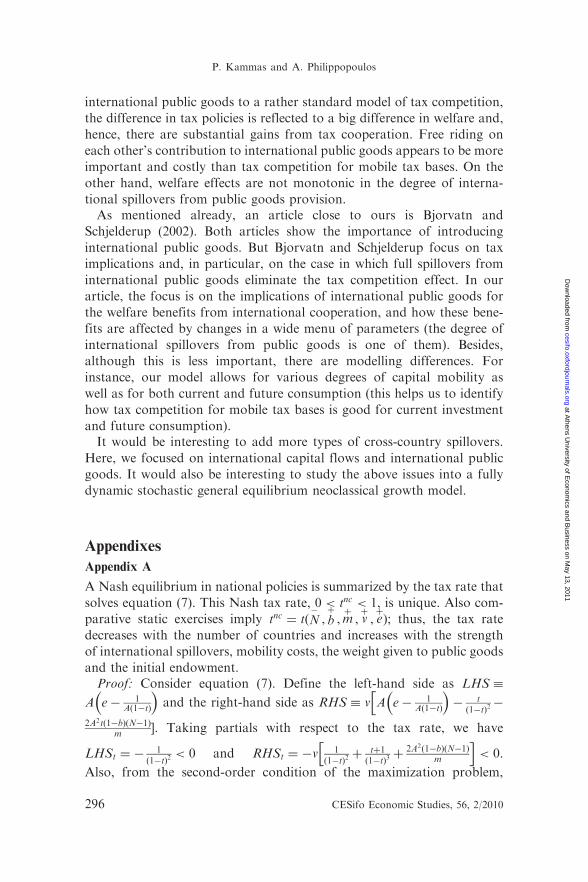
and the initial endowment.Proof: Consider equation (7). Define the left-hand side as LHS �
A e� 1Að1�tÞ
� �and the right-hand side as RHS � v A e� 1
Að1�tÞ
� �� tð1�tÞ2�
h2A2tð1�bÞðN�1Þ
m �. Taking partials with respect to the tax rate, we have
LHSt ¼ �1
ð1�tÞ2< 0 and RHSt ¼ �v
1ð1�tÞ2þ tþ1ð1�tÞ3þ
2A2ð1�bÞðN�1Þm
h i< 0.
Also, from the second-order condition of the maximization problem,
296 CESifo Economic Studies, 56, 2/2010
P. Kammas and A. Philippopoulos
at Athens U
niversity of Econom
ics and Business on M
ay 13, 2011cesifo.oxfordjournals.org
Dow
nloaded from
RHStj j > LHStj j for 0 < t < 1. Hence, assuming existence of a 0 < t < 1,
there is a unique solution tnc as illustrated in Figure A1.
In turn, total differentiation in equation (7) implies @tnc
@m ¼2A2tvðN�1Þð1�bÞm2ðLHSt�RHStÞ
,
which is non-negative since ðLHSt � RHStÞ > 0. Also, @tnc
@e ¼Aðv�1Þ
ðLHSt�RHStÞ,
which is positive when v > 1.
In addition, @tnc
@v ¼A e� 1
Að1�tÞ
� � t
ð1�tÞ2�
2A2 tðN�1Þð1�bÞm
h iLHSt�RHSt
¼ RHSvðRHSt�LHStÞ
and
@tnc
@b ¼2A2tvðN�1Þ
mðLHSt�RHStÞ, which are also positive. Finally, @tnc
@N ¼2A2tvðb�1Þ
mðLHSt�RHStÞ,
which is non-positive.
Appendix B
A cooperative equilibrium in national policies is summarized by the tax
rate that solves equation (8). This cooperative tax rate, 0 < tc < 1, is
unique. Also comparative static exercises imply tc ¼ tðNþ
, bþ
, vþ, eþÞ; thus,
the tax rate increases with the number of countries, the strength of inter-
national spillovers, the weight given to public goods and the initial endow-
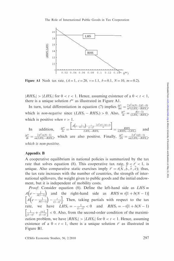
ment, but it is independent of mobility costs.Proof: Consider equation (8). Define the left-hand side as LHS �
A e� 1Að1�tÞ
� �and the right-hand side as RHS � v½1þ bðN� 1Þ�
A e� 1Að1�tÞ
� �� tð1�tÞ2
h i. Then, taking partials with respect to the tax
rate, we have LHSt ¼ �1
ð1�tÞ2< 0 and RHSt ¼ �v½1þ bðN� 1Þ
1ð1�tÞ2þ tþ1ð1�tÞ3
h i< 0. Also, from the second-order condition of the maximi-
zation problem, we have RHStj j > LHStj j for 0 < t < 1. Hence, assuming
existence of a 0 < t < 1, there is a unique solution tc as illustrated in
Figure B1.
0.02 0.04 0.06 0.08 0.1 0.12 0.14
10
12
14
16
18
20
RHS
LHS
(RH
S,L
HS)
(tnc)
Figure A1 Nash tax rate. (A¼ 1, e¼ 20, v¼ 1.1, b¼ 0.1, N¼ 10, m¼ 0.2).
CESifo Economic Studies, 56, 2/2010 297
The Role of International Public Goods in Tax Cooperation
at Athens U
niversity of Econom
ics and Business on M
ay 13, 2011cesifo.oxfordjournals.org
Dow
nloaded from

In turn, total differentiation in equation (8) implies @tc
@m ¼ 0,@tc
@e ¼Aðvðbþ1Þ�1ÞðLHSt�RHStÞ
, which is positive when v > 1bþ1.
In addition, @tc
@v ¼ ð1þ bðN� 1ÞÞA e� 1
Að1�tÞ
� � t
ð1�tÞ2
h iLHSt�RHSt
¼ RHSvðRHSt�LHStÞ
,
@tc
@b ¼ vðN� 1ÞA e� 1
Að1�tÞ
� � t
ð1�tÞ2
h iðLHSt�RHStÞ
and @tc
@N ¼ vbA e� 1
Að1�tÞ
� � t
ð1�tÞ2
h iðLHSt�RHStÞ
, which are all
positive.
References
Alesina, A. and R. Wacziarg (1999), ‘‘Is Europe is Going too Far?’’
Carnegie-Rocherster Conference Papers on Public Policy 51, 1–42.
Bjorvatn, K. and G. Schjelderup (2002), ‘‘Tax Competition with
International Public Goods’’, International Tax and Public Finance 9,
111–120.
Cooper, R. and A. John (1988), ‘‘Coordinating Coordination Failures in
Keynesian Models’’, Quarterly Journal of Economics 103, 441–463.
Devereux, M., B. Lockwood and M. Redoano (2008), ‘‘Do Countries
Compete over Corporate Tax Rates?’’ Journal of Public Economics 92,
1210–1235.
Kammas, P. and A. Philippopoulos (2007), ‘‘How Harmful is
International Tax Competition?’’, in G. Korres, ed., Regionalisation,
Growth, and Economic Integration, Physica-Verlag HD, Springer.
Mendoza, E. and L. Tezar (2005), ‘‘Why Hasn’t Tax Competition
Triggered a Race to the Bottom? Some Quantitative Lessons from the
EU’’, Journal of Monetary Economics 52, 163–204.
0.2 0.4 0.6 0.8
–10
10
20
30
40RHS
LHS
(tc)
(RH
S,L
HS)
Figure B1 Cooperative tax rate. (A¼ 1, e¼ 20, v¼ 1.1, b¼ 0.1, N¼ 10).
298 CESifo Economic Studies, 56, 2/2010
P. Kammas and A. Philippopoulos
at Athens U
niversity of Econom
ics and Business on M
ay 13, 2011cesifo.oxfordjournals.org
Dow
nloaded from
Persson, T. and G. Tabellini (1992), ‘‘The Politics of 1992: Fiscal Policyand European Integration’’, Review of Economic Studies 59, 689–701.
Persson, T. and G. Tabellini (1995), ‘‘Double-Edged Incentives:Institutions and Policy Coordination’’, in G. Grossman and K.Rogoff, eds., Handbook of International Economics, Volume 3, North-Holland, Amsterdam.
Philippopoulos, A. and G. Economides (2003), ‘‘Are Nash Tax Rates tooLow or too High? The Role of Endogenous Growth in Models withPublic Goods’’, Review of Economic Dynamics 6, 37–53.
Razin, A. and E. Sadka, eds., (1999), The Economics of Globalization:Policy Perspectives from Public Economics, Cambridge UniversityPress, Cambridge.
Sørensen, P. (2004), ‘‘International Tax Coordination: RegionalismVersus Globalism’’, Journal of Public Economics 88, 1187–1214.
Tabellini, G. (2003), ‘‘Principles of Policymaking in the EU: An EconomicPerspective’’, CESIFO Economic Studies 49, 75–102.
CESifo Economic Studies, 56, 2/2010 299
The Role of International Public Goods in Tax Cooperation
at Athens U
niversity of Econom
ics and Business on M
ay 13, 2011cesifo.oxfordjournals.org
Dow
nloaded from
Top Related