


Languages
Pages
Legal


The relationship between tax rates and budgetary
income. Adaptability of the Laffer curve in
budgetary planning
MASTER THESIS
Authors Academic Advisor
Sarunas Cerekas Erik Strøjer Madsen
MSc in Finance and International Business Department of Economics and
Business
Arturas Gumuliauskas
MSc in Finance and International Business
June 2012

Table of Contents
1. INTRODUCTION ................................................................................................................. 3
2. THEORY OF TAXES .......................................................................................................... 5
2.1. Tax history ...................................................................................................................... 5
2.2. Concept of taxes ............................................................................................................. 7
2.3. Classification of taxes ..................................................................................................... 8
2.4. Laffer Curve .................................................................................................................... 9
2.5. Personal Income Tax ..................................................................................................... 15
2.6. Value Added Tax ........................................................................................................... 17
3. TAX ANALYSIS ................................................................................................................. 21
3.1. GDP dynamics .............................................................................................................. 21
3.2. Budgetary dynamics ..................................................................................................... 26
3.3. Revenue composition ................................................................................................... 33
3.4. Income tax overview .................................................................................................... 35
3.5. VAT overview ............................................................................................................... 47
4. LABOR TAX REVENUE ESTIMATION ........................................................................... 56
4.1. Labor tax ratio determination ....................................................................................... 56
4.2. Labor tax revenue determination ................................................................................. 58
4.3. The Data ....................................................................................................................... 61
4.4. Model ........................................................................................................................... 62
4.5. Results .......................................................................................................................... 69
5. VAT REVENUE ESTIMATION ......................................................................................... 71
5.1. VAT Revenue Determination......................................................................................... 72
5.2. The Data ....................................................................................................................... 76
5.3. Model ........................................................................................................................... 78
5.3.1. Linear-Linear Model .................................................................................................. 79
5.3.2. Log- Log Model ......................................................................................................... 83
5.4. Results .......................................................................................................................... 86
6. CONCLUSION ................................................................................................................... 89
7. REFERENCES .................................................................................................................. 91

1. INTRODUCTION
"In this world nothing is certain but death and taxes."
--Benjamin Franklin, in a letter to M. Leroy, 1789.
Relying on these words of wisdom we should not fight taxes but learn to live
with them. History shows that changes in tax systems were common practice and
one can assume that the present system will continue to adopt changes based on
the state of public finances and extent of international trade, making the topic of
anticipating shift in taxation highly relevant. Taxes are the backbone of general
government revenue for countries across the globe and the imbalances between
revenue and expenditure often are the sources of political quarrels and economic
swings.
Due to the effects of globalization and free capital movement, which are
especially evident in economic and political unions, market participants are free to
choose the country of activity. Generally market participants are concerned with
the overall fiscal stability and tend to favor more stable countries. Countries with
the most significant or unexpected fiscal policy adjustments tend to be regarded as
slightly unstable and unpredictable, transforming them into risky markets with an
unattractive environment thus evoking the negative effect of capital flight from the
country.
Unsustainable levels of debt to GDP and budgetary deficits constitute a lethal
combination and have become a material topic for policy makers. Recent events
including the Greek debt restructuring deal, that was executed in March 2012 and
huge concerns aimed at similarly indebted South European countries of Portugal,
Italy and Spain raise the topic of austerity measures. Generally three ways of
budgetary balancing are used in practice: cuts in expenditures, increases in
revenues and borrowing, with the third option being the preferred choice of most

4 | P a g e
governments. However an initiative of fiscal austerity measures1 for most of the
European Union member states has been enacted on May 2012; it severely
curtailed the use of borrowing by general government, especially in the case of
member states that have and excessive and hardly sustainable debt to GDP ratio
of 60 %.
Since it is difficult to argue against the use of any of the two remaining
budgetary balancing measures, we will focus our thesis on the revenue maximising
measures that are at the disposal of individual countries. We identified the two
dominating taxes used by EU member states – labor tax and value added tax.
Each of the taxes will be estimated based on the Laffer theory of revenue
maximization. In theory Laffer Curve explains the parabolic relationship between
tax revenue and tax rate. The objective is to define the model for tax revenue to
see if the model is robust and fits with the theory of Laffer Curve. As a final result,
the revenue maximizing labor tax and value added tax rates will be computed and
compared to existing tax rates in different European countries.
The first section explores the basic theory of the taxes, including the concept of
the Laffer Curve. The second section presents the macroeconomic situation of the
sample countries and analyses labor tax and value added tax in more depth.
Finally, the models and estimations for both labor tax revenue and value added tax
revenue are estimated with the conclusions along with a summary presented at the
end of the paper.
1 Treaty on Stability, Coordination and Governance in the Economic and Monetary Union

5 | P a g e
2. THEORY OF TAXES
The Oxford dictionary states that a tax (Latin taxare: ‘to censure, charge,
compute‘) is a compulsory contribution to state revenue, levied by the government
on workers' income and business profits, or added to the cost of some goods,
services , and transactions. Taxes are not voluntary payments or donations in their
essence, but rather enforced contributions with failures to comply resulting in state
prosecution and punishment by law.
According to Meidūnas V., Puzinauskas (2001), no services or goods are
granted directly to the individual taxpayer for the payment of taxes. Funds are
accumulated and later dispensed through the budgetary mechanism according to
current National priorities. Budgetary expenditures exceeding revenue can only be
offset by borrowing or increasing tax rates, meaning that budgetary sustainability is
an essential element for the existence of a sovereign nation.
History shows that changes in tax systems were common practice and one can
assume that the present system will continue to adopt changes based on the state
of public finances and extent of international trade, making the topic of anticipating
shift in taxation highly relevant.
2.1. Tax history
Taxation can be considered as an integral part of society. With the evolution of
states came changes in the means of raising funds for military activities, expansion
and common social affairs (Meidūnas V., Puzinauskas, P, 2001). Taxes in all its
forms played a crucial role in the development of the modern state. The first
documented tax system was recorded in Ancient Egypt around 3000 BC, when
during a biennial event the Pharaoh would appear before his people and collect
taxes. Along with taxation came immunity from taxation to the privileged groups
with the first documented occurrence around 2600 BC for temple staff and the
property of temples and foundations.

6 | P a g e
Ancient Mesopotamian records provide more insight to the extent and methods
used in the primitive taxation systems. Due to the lack of a unified measure of
value, currently played by currency, taxes were paid in kind. Some periods saw
excessive taxation with a poll tax requiring each man to deliver a cow or a sheep to
the authorities, tolls and duties levied on the merchants required a portion of
transported goods to be paid. The most burdensome obligation frequently recorded
in history is the labor obligation, meaning that households were required to perform
certain deeds, including military service, for the state or local powers. A form of
labor obligation- serfdom- was common in Europe until its cancellation in late XIX
century, with obligations reaching 6 days of labor per week for every employable
household member.
Taxation levels varied depending on the state of public finance and in certain
countries displayed high levels of flexibility. In 167 BC due to successful expansion
and income generated from recently captured provinces, the Roman Empire
revoked the tax against land owned by its citizens in Italy. The Roman Empire also
practiced a novel approach to tax collection by introducing the model of private tax
collectors called ‘publicani’ at the expense of tax payers resulting in excess tax
rates.
As stated by Meidūnas V., Puzinauskas, (2001), the process of centralization of
political power in Europe that started in XV-XVI century caused serious financial
problems due to increased military, administrative and other expenses and was a
catalyst for change in taxation. The new movement, called mercantilism, focused
on enriching the state from international trade by decreasing taxation on exports
and increasing taxation on imports and laid the foundation of the basic principles of
modern customs and duty policies. Successive years saw growing concerns on the
topic of taxes with numerous proposals offered, from the Physiocratic position of a
single tax based on land ownership, since all the goods produced stem from land,
to the classical finance school position of minimizing taxes and the role of the state
altogether.
Two major schools of the modern economic thought on taxation are the ones of
Neo-Keynesian and Neo-classicists. The first movement envisions taxes as a

7 | P a g e
regulatory mechanism for manufacturing and industry and the tax system as an
anti-inflation and anti-recession model aimed at countering economic cycles and
thus smoothening economic swings. This is theoretically achieved by increasing
the tax burden and imposing additional constraints during the growth cycle and
contrary - decreasing the tax burden and increasing public expenditure during the
contraction cycle in the economy. The opposing economic school – the Neo-
classicists – holds a contradicting approach to taxes and believes in the self
regulating capabilities of the free market. According to them competition itself holds
the necessary regulatory power and the role of taxes and government in general
should be limited to warranting an effective balance of supply and demand and
ensuring local and national security (Stačiokas, R.,Rimas, J., 2003)
However taxation systems are constantly changing and the current model is
most likely simply a stage of the ongoing transition.
2.2. Concept of taxes
According to Stačiokas, R.,Rimas, J., (2003), taxes are the primary means of
funding public services such as security from external threats, internal policing and
sustaining public order, health care, social care, education, major infrastructure
projects, etc. Global practice shows that most of the public services cannot be
successfully outsourced through private businesses, since in many instances
projects might have negative net present value or the service might generate
insufficient return on investment. In the case of policing functions, privately owned
subjects might not be trustworthy with extremely fertile ground for corruption.
Generally it is difficult to evaluate the extent of public services consumed by
separate individuals, therefore common practice is taxation based on capability by
the subject.
In modern economics, fiscal policy and taxation rates can be a distortive
element. A lag factor exists in the administrative and functional level as well as in
the identification of economic cycles. This means that fiscal policy adjustments and
taxation rate changes require extensive discussion in the government level prior to

8 | P a g e
the decision. Substantial lag is also evident between the moment of resolution and
the actual effect that the resolution produces. Economic cycles are judged by major
macroeconomic rates such as inflation rates and Gross Domestic Product (GDP)
rates which by themselves are lagging indicators. Therefore reacting to economic
cycles through fiscal changes presents significant challenges and has the power to
trigger severe budgetary constraints.
2.3. Classification of taxes
In modern times individual taxes are composed of five essential elements
(classification supplied by Meidūnas V., Puzinauskas, P, 2001):
• A tax subject is a person who is assigned the obligation to pay taxes.
Commonly the tax subject and the actual tax payer are congruous, but in
certain cases they might not coincide (in the case of value added tax, the tax
subject is the consumer of the product, but the payer is the seller of the
product).
• A tax object is the actual object that is being taxed like income, services,
goods, assets, etc.
• The unit of taxation is a unit of measurement that is required for the estimation
of the amount of tax payable, like a currency unit for income tax, a hectare for
land taxes, capacity for excise duties.
• The tax rate is amount of tax required per unit of taxation. Usually the tax rate
is expressed in a percentage value (income tax, goods and services tax), it can
also be expressed as a fixed amount (diesel, tobacco).
• A tax exemption is a special tax rate reduction for certain tax subjects. Tax
exemptions may be temporary or permanent, compulsory or allowable. A tax
credit (a delay of payments) and tax holiday (a waiver of taxes for a certain
period of time) are both forms of tax exemption.
In modern tax theory, taxes are broadly categorized into two branches- direct
and indirect taxes. The distinction is made based on tax object and the relation

9 | P a g e
between the tax subject and state- directly from income and assets or indirectly
from the price system (added to the price of goods sold within a state). Classifying
individual taxes into these major branches is a fairly subjective matter because
most direct taxes like corporate revenue taxes can be argued to be transferable to
the consumer in the pricing process, but the dominant classification is common and
based on best practice.
The most widespread direct tax is the income tax, levied on personal income
and corporate revenue. Other examples of direct taxes are property taxes, land
taxes, inheritance taxes, capital, capital gains taxes and other. The most common
indirect taxes are levied on goods and services, like the Value Added Tax, the
Goods and Sales Tax and other taxes that actually fall on the consumer but are
paid by the seller, like excise duties on oil products, alcohol, tobacco and other
goods that are generally regulated by the government or belong to monopolist
industries.
A different type of tax is the Ecological tax, the subject of which is the
consumption of polluting materials like most oil products. The tax revenue is not
directed to the national or municipal budgets but is rather accumulated for dealing
with prevention and consequences of pollution. Another specific tax exists in the
European Union and is levied on the imports of agricultural products, the proceeds
of which are directed to the EU budget.
In our thesis we will focus on two major taxes- one from each branch- personal
income tax and Value Added Tax. The particular taxes were chosen based on their
prevalence globally and the extent of budgetary income they generate.
2.4. Laffer Curve
As the stagflation, high unemployment and high inflation appeared in the 1970s,
demand side policies were unable to solve such type of the problems (van Duijn,
1982). However, supply-side economists believed that the reason for stagflation is
an excessive tax burden and an economical over-regulation by the government. In

10 | P a g e
order to solve stagflation problem, the policy of a tax reduction and a deregulation
of the economy must be pursued (Burda, Wyplosz, 1993). Supply
expressed in the Laffer curve which depicts the expected rel
revenue and tax rate.
The Laffer curve is named after economist Art Laffer, who is said to have drawn
this curve on a napkin in a Washington restaurant in 1974. The Laffer curve states
that there is parabolic relationship between tax
noted, “there are always two tax rates that yield the same revenues” (Laffer, 1986).
That means that taxable income changes when tax rate is altered, but there is a
point where reduction in taxable income from higher ta
enough to completely offset the higher tax rate. This point is called “revenue
maximizing” point.
Laffer curve is the illustration of a dynamic scoring model (Fig
scoring model (Figure 1a) assumes that the higher the ta
revenue is collected. One can contradict that if tax rate was 100 per cent, no one
would work and thus no tax revenue would be collected. Also, if tax rate was 0 per
cent, obviously no tax revenue would be collected as well. This lead
that relationship between tax rate and tax revenue must be parabolic.
Figure 1. Comparison of the static scoring and dynamic scoring.
order to solve stagflation problem, the policy of a tax reduction and a deregulation
of the economy must be pursued (Burda, Wyplosz, 1993). Supply
expressed in the Laffer curve which depicts the expected relationship between tax
The Laffer curve is named after economist Art Laffer, who is said to have drawn
this curve on a napkin in a Washington restaurant in 1974. The Laffer curve states
that there is parabolic relationship between tax rates and tax revenue. As Art Laffer
noted, “there are always two tax rates that yield the same revenues” (Laffer, 1986).
That means that taxable income changes when tax rate is altered, but there is a
point where reduction in taxable income from higher tax rates becomes large
enough to completely offset the higher tax rate. This point is called “revenue
Laffer curve is the illustration of a dynamic scoring model (Fig
igure 1a) assumes that the higher the tax rate the higher tax
revenue is collected. One can contradict that if tax rate was 100 per cent, no one
would work and thus no tax revenue would be collected. Also, if tax rate was 0 per
cent, obviously no tax revenue would be collected as well. This lead
that relationship between tax rate and tax revenue must be parabolic.
. Comparison of the static scoring and dynamic scoring.
order to solve stagflation problem, the policy of a tax reduction and a deregulation
of the economy must be pursued (Burda, Wyplosz, 1993). Supply-side ideas are
ationship between tax
The Laffer curve is named after economist Art Laffer, who is said to have drawn
this curve on a napkin in a Washington restaurant in 1974. The Laffer curve states
rates and tax revenue. As Art Laffer
noted, “there are always two tax rates that yield the same revenues” (Laffer, 1986).
That means that taxable income changes when tax rate is altered, but there is a
x rates becomes large
enough to completely offset the higher tax rate. This point is called “revenue-
Laffer curve is the illustration of a dynamic scoring model (Figure 1b). Static
x rate the higher tax
revenue is collected. One can contradict that if tax rate was 100 per cent, no one
would work and thus no tax revenue would be collected. Also, if tax rate was 0 per
cent, obviously no tax revenue would be collected as well. This leads to a notion
that relationship between tax rate and tax revenue must be parabolic.

11 | P a g e
Laffer assumes that too high tax rates make people to be inactive
Figure 2 illustrates extreme occasion when tax rate is 100 per cent. High taxation
rate leads to low production, low incomes and, consequently, to low tax revenues
(Heijman, van Ophem, 2005). Additionally, people may become active in the black
labor economy. As Friedman et al
are generally correlated with a higher share of the unofficial economy. Lower tax
rates, conversely, make people to withdraw from the black economy and become
officially active. Point B in Figure 2 shows “reve
government can reach optimum tax rate and collect maximum possible tax
revenue.
Figure 2. Laffer Curve
As Mitchell (2009) argues revenue maximizing point is not the best for whole
economy. Ideal policy is reached in growth max
somewhere on upward sloping section of the Laffer curve. Growth maximizing
point is greater than zero, because there is a need for tax revenue to ensure
market economy function. Society needs such things as public safety,
courts, and healthcare.
The Laffer curve explains relationship between tax rate and tax revenue.
However, in the real world tax rate changes are not made in isolation with other
economic aspects. Beczi (2000) analyses what happens if the government
Laffer assumes that too high tax rates make people to be inactive
extreme occasion when tax rate is 100 per cent. High taxation
rate leads to low production, low incomes and, consequently, to low tax revenues
(Heijman, van Ophem, 2005). Additionally, people may become active in the black
labor economy. As Friedman et al (Friedman et al, 2000) shows, higher tax rates
are generally correlated with a higher share of the unofficial economy. Lower tax
rates, conversely, make people to withdraw from the black economy and become
officially active. Point B in Figure 2 shows “revenue-maximizing” level where
government can reach optimum tax rate and collect maximum possible tax
As Mitchell (2009) argues revenue maximizing point is not the best for whole
economy. Ideal policy is reached in growth maximizing point (Figure 2), which is
somewhere on upward sloping section of the Laffer curve. Growth maximizing
point is greater than zero, because there is a need for tax revenue to ensure
market economy function. Society needs such things as public safety,
The Laffer curve explains relationship between tax rate and tax revenue.
However, in the real world tax rate changes are not made in isolation with other
economic aspects. Beczi (2000) analyses what happens if the government
Laffer assumes that too high tax rates make people to be inactive – Point C in
extreme occasion when tax rate is 100 per cent. High taxation
rate leads to low production, low incomes and, consequently, to low tax revenues
(Heijman, van Ophem, 2005). Additionally, people may become active in the black
(Friedman et al, 2000) shows, higher tax rates
are generally correlated with a higher share of the unofficial economy. Lower tax
rates, conversely, make people to withdraw from the black economy and become
maximizing” level where
government can reach optimum tax rate and collect maximum possible tax
As Mitchell (2009) argues revenue maximizing point is not the best for whole
imizing point (Figure 2), which is
somewhere on upward sloping section of the Laffer curve. Growth maximizing
point is greater than zero, because there is a need for tax revenue to ensure
market economy function. Society needs such things as public safety, honest
The Laffer curve explains relationship between tax rate and tax revenue.
However, in the real world tax rate changes are not made in isolation with other
economic aspects. Beczi (2000) analyses what happens if the government actively

12 | P a g e
spend its revenues, as it is obvious in the real world. If the government spends
more revenues on taxed goods, it will increase the demand for good. This action
will offset the decrease in tax revenue caused by tax increase. Therefore, revenue
maximizing tax rate will rise. In Figure 3 one can see that because of demand
curve shift, revenue-maximizing tax rate moves from Point A to Point E. Finally
Beczi (2000) concludes that if government cuts taxes and at the same time rises
government consumption and decreases public investments, it increases the
likelihood that optimal tax revenues are lost. Tax policy must be related to both
public investment and public spending.
Figure 3. The impact on tax rate due to demand curve shift.
Furthermore, Henderson (1981) points out interesting idea that real
curve is more complex. It looks like in Figure 4, because, as Henderson argues,
tax rate cut would not necessarily cause people to work more.
spend its revenues, as it is obvious in the real world. If the government spends
more revenues on taxed goods, it will increase the demand for good. This action
will offset the decrease in tax revenue caused by tax increase. Therefore, revenue
ximizing tax rate will rise. In Figure 3 one can see that because of demand
maximizing tax rate moves from Point A to Point E. Finally
) concludes that if government cuts taxes and at the same time rises
on and decreases public investments, it increases the
likelihood that optimal tax revenues are lost. Tax policy must be related to both
public investment and public spending.
The impact on tax rate due to demand curve shift.
Furthermore, Henderson (1981) points out interesting idea that real
curve is more complex. It looks like in Figure 4, because, as Henderson argues,
tax rate cut would not necessarily cause people to work more.
spend its revenues, as it is obvious in the real world. If the government spends
more revenues on taxed goods, it will increase the demand for good. This action
will offset the decrease in tax revenue caused by tax increase. Therefore, revenue-
ximizing tax rate will rise. In Figure 3 one can see that because of demand
maximizing tax rate moves from Point A to Point E. Finally
) concludes that if government cuts taxes and at the same time rises
on and decreases public investments, it increases the
likelihood that optimal tax revenues are lost. Tax policy must be related to both
Furthermore, Henderson (1981) points out interesting idea that real-life Laffer
curve is more complex. It looks like in Figure 4, because, as Henderson argues,

13 | P a g e
Figure 4. Complex shape of the
If the government cuts tax rate, tax revenues move from point A to point B.
People get higher income because of tax cut, but they might work less and spend
more time for leisure. Therefore, tax revenues decrease.
Another aspect, discussed by
which is also a tax. If tax rate cut does not cause immediate rise of tax revenue
and government does not decrease spending, the increase in budget deficit will
appear. Therefore, in countries, which have
would increase. Also increase in tax revenues might appear simpl
population growth.
Feige, Edgar L., and Robert T. McGee (1982) developed a simple model for
Laffer curve. The model shows that the shape and
Sweden depend on the power supply, the progressivity of the tax system and the
size of the observed economy.
Jonas Agell and Mats Persson (2000) analyze the government budget balance
in a simple endogenous growth model, by
transfer-adjusted tax rates in OECD countries to determine if countries apply
theoretically optimal tax rates. Jesús Alfonso Novales and Ruiz (2002) analyze
Complex shape of the Laffer Curve.
If the government cuts tax rate, tax revenues move from point A to point B.
People get higher income because of tax cut, but they might work less and spend
more time for leisure. Therefore, tax revenues decrease.
Another aspect, discussed by Henderson, is that tax cut can increase inflation,
which is also a tax. If tax rate cut does not cause immediate rise of tax revenue
and government does not decrease spending, the increase in budget deficit will
appear. Therefore, in countries, which have the power of currency issue, inflation
would increase. Also increase in tax revenues might appear simpl
Feige, Edgar L., and Robert T. McGee (1982) developed a simple model for
Laffer curve. The model shows that the shape and position of the Laffer curve for
Sweden depend on the power supply, the progressivity of the tax system and the
size of the observed economy.
Jonas Agell and Mats Persson (2000) analyze the government budget balance
in a simple endogenous growth model, by conducting an empirical study of
adjusted tax rates in OECD countries to determine if countries apply
theoretically optimal tax rates. Jesús Alfonso Novales and Ruiz (2002) analyze
If the government cuts tax rate, tax revenues move from point A to point B.
People get higher income because of tax cut, but they might work less and spend
Henderson, is that tax cut can increase inflation,
which is also a tax. If tax rate cut does not cause immediate rise of tax revenue
and government does not decrease spending, the increase in budget deficit will
the power of currency issue, inflation
would increase. Also increase in tax revenues might appear simply because of
Feige, Edgar L., and Robert T. McGee (1982) developed a simple model for
position of the Laffer curve for
Sweden depend on the power supply, the progressivity of the tax system and the
Jonas Agell and Mats Persson (2000) analyze the government budget balance
conducting an empirical study of
adjusted tax rates in OECD countries to determine if countries apply
theoretically optimal tax rates. Jesús Alfonso Novales and Ruiz (2002) analyze

14 | P a g e
how to manage deficit by substituting debt with taxes. They find that tax cuts on
labor and capital income have a positive effect on growth rate of the economy.
Trabandt Mathias and Harald Uhlig (2006) used a neoclassical growth model,
calibrated with constant Frisch elasticity for the US, and EU-14 economy. The
results show that both US and EU-14 economies can increase tax rates on labor
and capital income and gain higher tax revenues. However the Laffer curve in
consumption taxes does not have a peak.
The discussion about implementation of the Laffer curve in practice spread
widely in the USA in 1970’s. At that time top federal tax rate was 70 per cent and
encouraged people from that tax bracket to withdraw from official economy.
Proponents of the Laffer curve suggested politicians to cut tax rate and collect
higher tax revenues. Finally in 1988 top tax rate dropped to 28 per cent leading to
the increase of tax revenue five times as much revenue as was collected when top
tax rate was 70 per cent2. Table 1 shows that the number of tax payers (who’s
income was over $200 000) was nearly 117 000 and tax paid was more than $19
billion. After tax cut the number of the taxpayers in that bracket jumped to nearly
724 000 and the government collected more than $99 billion of taxes. However one
needs take into account the facts that population grew over this period as well as
inflation increased about 44 per cent. Still this example illustrates strong effect of
the Laffer curve.
Taxes paid on income over $200 000 in 1980
Tax bracket Number of
taxpayers
Taxable
income Income tax paid
$200 000 - $500 000 99 971 $22 696 007 $11 089 114
$500 000 - $1 000 000 12 379 $6 512 424 $3 613 195
$1 000 000 and more 4 389 $7 013 225 $4 301 111
Total 116 757 $36 221 656 $19 003 420
Taxes paid on income over $200 000 in 1988
Tax bracket Number of Taxable Income tax paid
2 http://www.irs.gov/taxstats/indtaxstats/article/0,,id=96981,00.html

15 | P a g e
$200 000 - $500 000
$500 000 - $1 000 000
$1 000 000 and more
Total
Table 1. Labor tax statistics in the USA
Another example is Ireland. In 1985 with corporate tax rate of 50 per cent
Ireland collected tax revenues equal to 1.1 per cent of GDP
steadily decreased corporate tax rate until it was 12.5 per cent in 2000. As shown
in Figure 5, corporate tax revenues increased about three times and reached 3.6
percent of GDP. It must be noted that GDP figures are corrected for inflatio
Laffer curve effect is obvious in this case.
Figure 5. Corporate Tax Rate and Corporate Tax Revenue dynamics in Ireland.
2.5. Personal Income Tax
Personal Income Tax is a direct tax levied on income of a person. A person
means an individual, an
Generally, a person pay tax calendar year basis.
3 http://www.oecd.org.dataoecd/48/27/41498733.pdf
taxpayers income
547 239 $134 655 949
114 562 $67 552 225
61 896 $150 744 777
723 697 $352 952 951
Labor tax statistics in the USA
Another example is Ireland. In 1985 with corporate tax rate of 50 per cent
Ireland collected tax revenues equal to 1.1 per cent of GDP3. The government
steadily decreased corporate tax rate until it was 12.5 per cent in 2000. As shown
, corporate tax revenues increased about three times and reached 3.6
percent of GDP. It must be noted that GDP figures are corrected for inflatio
Laffer curve effect is obvious in this case.
Corporate Tax Rate and Corporate Tax Revenue dynamics in Ireland.
Personal Income Tax
Personal Income Tax is a direct tax levied on income of a person. A person
means an individual, an ordinary partnership, a non-juristic body of person.
Generally, a person pay tax calendar year basis.
http://www.oecd.org.dataoecd/48/27/41498733.pdf
$38 446 620
$19 040 602
$42 254 821
$99 742 043
Another example is Ireland. In 1985 with corporate tax rate of 50 per cent
. The government
steadily decreased corporate tax rate until it was 12.5 per cent in 2000. As shown
, corporate tax revenues increased about three times and reached 3.6
percent of GDP. It must be noted that GDP figures are corrected for inflation. So
Corporate Tax Rate and Corporate Tax Revenue dynamics in Ireland.
Personal Income Tax is a direct tax levied on income of a person. A person
juristic body of person.

16 | P a g e
Taxpayers are classified into residents and non-residents. The definition of a
concept “resident” differs from country to country. Basically, “resident” means any
person residing in certain country for a certain period of time. A resident of certain
country is liable to pay tax on income from sources both in the country he/she
resides and in foreign countries. A non-resident is a person who does not reside in
certain country but still earns income in that country.
Income can be in cash and in kind. Both of these income types are chargeable
to the personal income tax. The income which is subject to income taxation is
called assessable income. Certain deductions and allowances are allowed in the
calculation of the taxable income. Taxpayer shall make deductions from
assessable income before the allowances are granted. Therefore, taxable income
is calculated by the following formula:
Taxable income = Assessable Income - deductions - allowances
Taxes can have a significant effect on income distribution in an economy. As
Adam Smith (1904) noted tax should be linked to ability to pay. Therefore, tax
systems can be distinguished as follows:
• Progressive tax system – a system in which tax represents a greater proportion
of a person's income as their income rises. In other words, the average rate of
taxation rises.
• Regressive tax system – a system in which tax represents a smaller proportion
of a person's income as their income rises. In other words, the average rate of
taxation falls.
• Proportional tax system – a system in which tax is paid as the percentage if the
income. The percentage remains the same despite the level of income. In this
system the average rate of taxation is constant.
There is always an open discussion about the difficulties in administering the
tax and maintaining a sense of fairness of who is paying and how much. Proposals
to modify the income tax system to make it “flat” (fewer tax rates and fewer
deductions) arise more often (Kiefer, 2010). Still, income tax is an important source
of budgetary income. However, each country has its own specifics on personal

17 | P a g e
income tax. The review of personal income tax along with labor taxes are depicted
in Section 3.4.
2.6. Value Added Tax
Value added tax (VAT) is one of the most widespread indirect taxes in the world
with increasingly more countries adopting it for taxation of consumption. According
to the Organization of Economic Cooperation and Development (OECD), over 150
countries have implemented a VAT/GST and there is a need for a global platform
where the economic, social and cross border issues of operating a VAT/GST can
be discussed. A VAT is levied on the difference between a business’s sales and
its purchases of goods and services. Typically, a business calculates the tax due
on its sales, subtracts a credit for taxes paid on its purchases, and remits the
difference to the government (United States Accountability Office Report to
Congressional Requests, Value Added Taxes, 2008.)
The Lithuanian Ministry of Finance proposes the following definition of the VAT
subject: ‘the subject of VAT is the supply of goods and services by a taxable
person in the performance of his/its economic activities within the territory of the
country that are affected for consideration’. The value added tax system is
designed to address various problems associated with the conventional sales tax
system such as cascading- the term describing a situation when the end consumer
of a product is obliged to pay taxes on an input that has already been taxed earlier
in the production chain. The clarity and transparency of the VAT system enables
effective elimination of the cascade problem and the associated tax evasion
problem. In regard of International trade, VAT is seen by some countries as
discriminatory. The American Manufacturing Trade Action Coalition (AMTAC)
express concerns that the rebate of taxes upon export normally is prohibited under
the World Trade Organization trading regime, but within the Value Added Tax
system, taxes are rebated on exports and assessed on imports, triggering
International imbalances and providing certain countries with a competitive
advantage. According to the OECD, research suggests that the current

18 | P a g e
international environment for consumption taxes, especially with respect to trade in
services and intangibles, is hindering business activity and economic growth and
distorts competition. The US Government Accountability Office also discusses
initiatives of introducing a VAT equivalent in the US. The creation of a global
framework for applying VAT/GST on international trade is therefore a key priority
for the OECD.
Our Master thesis will be primarily focused on members of the European Union
therefore the European VAT systems will be addressed in more depth. VAT was
invented in 1954 by a French economist and introduced by Maurice Laure, the joint
director of the French tax authority. It was introduced for large businesses but later
expanded to remaining sectors of the economy. On 11 April 1967 the first two VAT
Directives were adopted, establishing a general, multi-stage but non-cumulative
turnover tax to replace all other turnover taxes in the Member States. The first two
VAT Directives laid down only the general structures of the system with Member
States being free to determine the VAT coverage. In May 1977 the Sixth VAT
Directive was adopted and established a uniform VAT coverage. On 1 January
2007, the Sixth Directive was replaced by the VAT Directive which guarantees that
the VAT contributed by each of the Member States to the Community's own
resources can be calculated. It still however, allows Member States many possible
exceptions and derogations from the standard VAT coverage. Moreover, it does
not set out the rates of VAT to be applied in Member States, only a minimum rate
of 15%. For transactions between taxable persons it is still a destination based
VAT system, but it is a Transitional VAT System, and the intention is eventually to
have a common system of VAT where VAT is charged by the seller of goods - an
origin based VAT system with VAT being charged at the rate in force where the
supplier is established4.
The European e-Justice portal under the European Commission provides the
following explanation of a VAT system: ‘The common system of VAT applies to the
production and distribution of goods and services bought and sold for consumption
4 European Commission on the history of value added taxes in Europe

19 | P a g e
within the European Union and the actual tax burden is visible at each stage in the
production and distribution chain. To ensure that the tax is neutral in impact,
irrespective of the number of transactions, taxable persons for VAT may deduct
from their VAT account the amount of tax which they have paid to other taxable
persons. VAT is finally borne by the final consumer in the form of a percentage
addition to the final price of the goods or services’. Double taxation is avoided and
tax is paid only on the value added at each stage of production and distribution. In
this way, as the final price of the product is equal to the sum of the values added at
each preceding stage, the final VAT paid is made up of the sum of the VAT paid at
each stage. The tax is paid to the revenue authorities by the seller of the goods,
who is the taxable person, but it is actually paid by the buyer to the seller as part of
the price thus making it an indirect tax.
For VAT purposes, a taxable person is any individual, partnership, company or
any other subject which supplies taxable goods and services in the course of
business. However, if the annual turnover of this person is less than a certain limit
(the threshold), which differs according to the Member State, the person does not
have to register as a payer and charge VAT on their sales. EU Member States
have freedom of choice setting the values of thresholds for VAT registration and for
the minimum standard and reduced rates as long as they comply with the minimum
requirements. Supplies of goods and services subject to VAT are normally subject
to a standard rate of at least 15% but Member States may apply one or two
reduced rates of not less than 5% to goods and services enumerated in a restricted
list. However, these rules are complicated by a multitude of derogations granted to
certain Member States which were granted during the negotiations preceding the
adoption of the VAT rates Directive of 1992 and in the Acts of Accession to the
European Union. Such derogations prevent a coherent system of VAT rates in the
EU from being applied.
In order to eliminate any competitive disadvantages stemming from tax rate
differences between Member states and for the purpose of exports between the
Community and non-member countries, no VAT is charged on the transaction and
the VAT already paid on the inputs of the good for export is deducted - this is an

20 | P a g e
exemption with the right to deduct the input VAT. There is thus no residual VAT
contained in the export price. However, as far as imports are concerned, VAT must
be paid at the moment the goods are imported so they are immediately placed on
the same footing as equivalent goods produced in the Community. Taxable people
registered for VAT will be allowed to deduct this VAT in their next VAT return5 The
significance of value added tax proceeds in European Union member states both in
its nominal form and as a proportion of total tax revenue with associated
implications will be discussed in a later chapter of the thesis.
5 The European e-Justice Portal under the European Commission,
http://ec.europa.eu/taxation_customs/index_en.htm
21 | P a g e
3. TAX ANALYSIS
Differing taxation policies and trends, as well as the political and business
environment, are basic factors affecting the level of competitiveness of countries.
As was already mentioned, consistency in countries‘ economic and taxation policy
is of vital importance to the subjects pursuing business objectives both in their
home markets and abroad. Specific data on the dynamics of national budgetary
revenue, the composition of the revenue depending on specific taxes, levels of
expenditure and borrowing should be addressed in order to substantiate the
problem of possible tax changes Europe-wide.
We will present a basic overview of the present-day European Union member
states Gross Domestic Product (GDP) dynamics, revenue and expenditure levels
of the general government and analyze the composition of revenue and its trends.
General government data will be used as an aggregate proxy allowing us to
perform country level comparison and bypass the variations in the extent of
centralization, municipal taxation and compulsory social welfare charges.
3.1. GDP dynamics
Gross domestic product is a measure of the economic activity, defined as the
value of all goods and services produced less the value of any goods or services
used in their creation. It is important to review the extent of and dynamics of
economic activity in all the EU member states and grasp the underlying differences
between them. Due to limited availability of valid statistical data for the full sample,
only the period of 1996-2011 will be reviewed in this section.
Table 2 demonstrates the significant disparity of nominal GDP growth in the EU
member states from year 1996 to 2011 with 1996 as the base year. As visible in
the table, the greatest growth was displayed by member states that were admitted
during the final two enlargement stages with exceptionally high figures
demonstrated by the former states of the Soviet Union and its satellites of the
Warsaw Pact. The economies of these highly dynamic countries are extremely

22 | P a g e
sensitive to economic and fiscal policy changes and represent a potential obstacle
in the homogenization of the tax environment. The column depicting nominal GDP
change in national currency for the Euro Zone countries is calculated as Euro-fixed
series by applying the Euro fixed rate on the national currencies data with
discrepancies of the GDP change data compared to nominal GDP change in Euros
stemming from the pre-Euro exchange rate fluctuations. The column is intended to
display the heterogeneity of the economies of the member states with Romania
and Bulgaria having recently experienced a period of significant inflation, and
Czech Republic, Slovakia and Lithuania appreciating the value of their currencies
during the period of 1996-2011. Furthermore, while Czech Republic and Slovakia
(Slovakia joined the Euro Zone in January 1st 1999) have evolved from a pegged
currency rate to a managed and eventually floating exchange rate with its positive
effects on the economy and trade, Lithuania achieved the depreciation by merely
swapping the base currency used for the peg from US Dollar to the Euro. This
means that even in this respect the three countries are not readily comparable.
Country
Nominal GDP
Change, EUR
Nominal GDP
Change, National currency Country
Nominal GDP
Change, EUR
Nominal GDP
Change, National currency
Belgium 69,81% 74,00% Luxembourg 157,65% 171,08%
Bulgaria 386,28% 4173,53% Hungary 178,51% 301,56% Czech Republic 203,02% 116,24% Malta 121,08% 107,37% Denmark 65,23% 67,04% Netherlands 82,84% 88,30% Germany 33,86% 37,11% Austria 62,92% 66,87% Estonia 328,82% 339,11% Poland 199,36% 260,92% Ireland 165,47% 163,50% Portugal 79,24% 83,46% Greece 96,01% 118,59% Romania 370,21% 4982,06% Spain 118,85% 126,52% Slovenia 113,84% 198,32% France 60,40% 62,05% Slovakia 314,47% 220,79% Italy 58,42% 56,59% Finland 89,43% 93,25% Cyprus 143,22% 140,49% Sweden 77,77% 88,52%
Latvia 348,25% 352,54% United Kingdom 81,08% 92,85%
Lithuania 362,62% 214,54% Table 2. Nominal GDP growth in 1996-2011

23 | P a g e
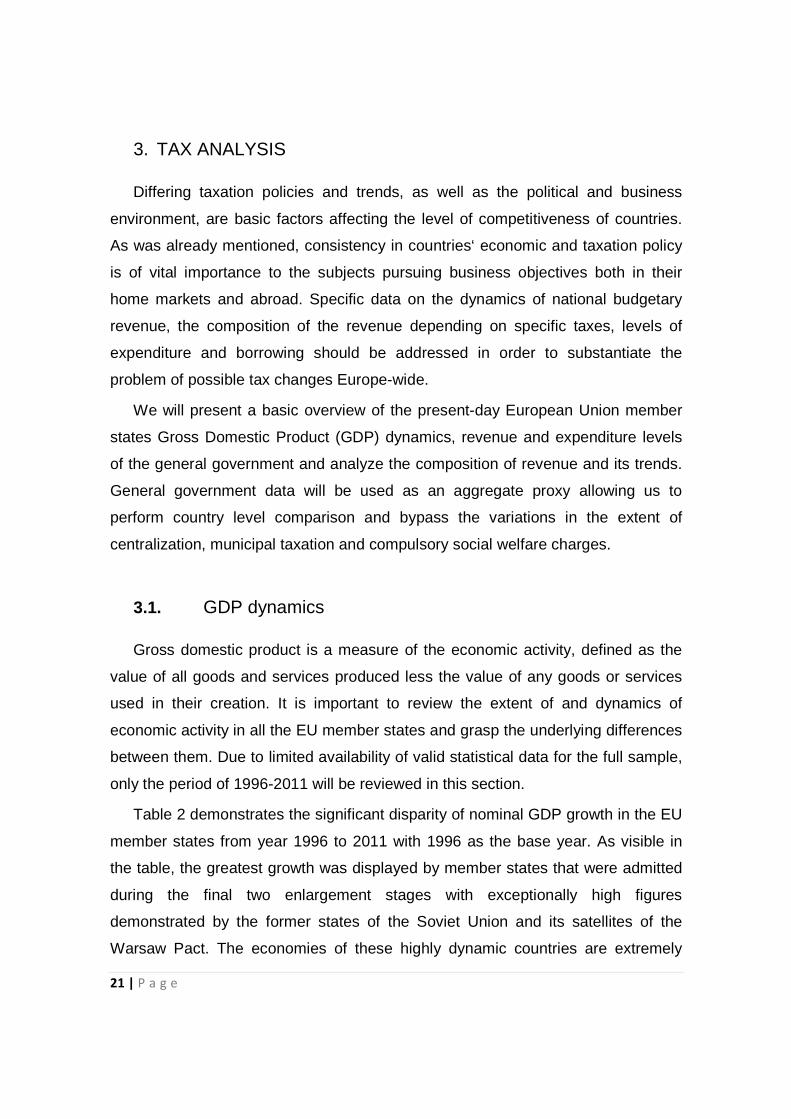
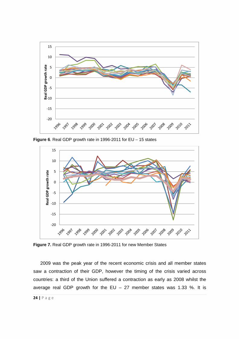
Figures 6 and 7 have intentionally been projected on a uniform vertical axis
range to depict the real GDP growth rate for year 1996 to 2011 for two groups of
countries based on the years of accession to the European Union. The duration of
membership is likely to reflect the qualitative effect resulting from prolonged
exposure to the unified market conditions, broader experience in the competitive
market setting and the inveteracy of democratic rule and correspondent values.
The first group consists of the EU – 15 countries that have been member states
during the whole sample period and the second group is comprised of countries
admitted during the latest stages of EU enlargement most of which have
experienced a transition to the competitive market setting during the sample
period. The calculation of the annual growth rate of GDP volume is intended to
allow comparisons of the dynamics of economic development both over time and
between economies of different sizes. For measuring the growth rate of GDP in
terms of volumes, the GDP at current prices are valued in the prices of the
previous year and the thus computed volume changes are imposed on the level of
a reference year. This type of measurement eliminates the effects of price changes
during the period and allows for adequate comparison. Among the EU – 15
member states Ireland and Luxembourg initially demonstrated a higher growth rate
in and Greece experienced significant contraction in the end of the period. The 12
EU member states that have joined the Union during the last stages of
enlargement are depicted individually with the bold line representing the average
arithmetical real GDP growth rate for the 15 EU countries. The three newly
independent Baltic states of Lithuania, Latvia and Estonia have experienced the
greatest fluctuations in the growth rate with Malta and Cyprus showing generally
milder deviations and Poland demonstrating a sustainably higher growth rate with
increased resilience to significant changes.
24 | P a g e
Figure 6. Real GDP growth rate in 1996-2011 for EU – 15 states
Figure 7. Real GDP growth rate in 1996-2011 for new Member States
2009 was the peak year of the recent economic crisis and all member states
saw a contraction of their GDP, however the timing of the crisis varied across
countries: a third of the Union suffered a contraction as early as 2008 whilst the
average real GDP growth for the EU – 27 member states was 1.33 %. It is
-20
-15
-10
-5
0
5
10
15R
ea
l G
DP
gro
wth
ra
te
-20
-15
-10
-5
0
5
10
15
Re
al
GD
P g
row
th r
ate
25 | P a g e
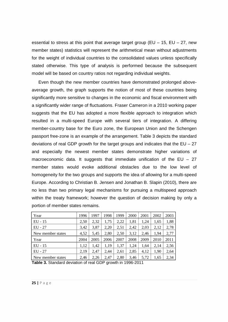
essential to stress at this point that average target group (EU – 15, EU – 27, new
member states) statistics will represent the arithmetical mean without adjustments
for the weight of individual countries to the consolidated values unless specifically
stated otherwise. This type of analysis is performed because the subsequent
model will be based on country ratios not regarding individual weights.
Even though the new member countries have demonstrated prolonged above-
average growth, the graph supports the notion of most of these countries being
significantly more sensitive to changes in the economic and fiscal environment with
a significantly wider range of fluctuations. Fraser Cameron in a 2010 working paper
suggests that the EU has adopted a more flexible approach to integration which
resulted in a multi-speed Europe with several tiers of integration. A differing
member-country base for the Euro zone, the European Union and the Schengen
passport free-zone is an example of the arrangement. Table 3 depicts the standard
deviations of real GDP growth for the target groups and indicates that the EU – 27
and especially the newest member states demonstrate higher variations of
macroeconomic data. It suggests that immediate unification of the EU – 27
member states would evoke additional obstacles due to the low level of
homogeneity for the two groups and supports the idea of allowing for a multi-speed
Europe. According to Christian B. Jensen and Jonathan B. Slapin (2010), there are
no less than two primary legal mechanisms for pursuing a multispeed approach
within the treaty framework; however the question of decision making by only a
portion of member states remains.
Year 1996 1997 1998 1999 2000 2001 2002 2003
EU - 15 2,50 2,32 1,75 2,22 1,81 1,24 1,65 1,88
EU - 27 3,42 3,87 2,20 2,51 2,42 2,03 2,12 2,78
New member states 4,52 5,45 2,80 2,50 3,12 2,46 1,94 2,77
Year 2004 2005 2006 2007 2008 2009 2010 2011
EU - 15 1,12 1,42 1,19 1,37 1,24 1,64 2,14 2,56
EU - 27 2,19 2,47 2,44 2,61 2,85 4,12 1,90 2,64
New member states 2,46 2,26 2,47 2,80 3,46 5,72 1,65 2,34 Table 3. Standard deviation of real GDP growth in 1996-2011

26 | P a g e
3.2. Budgetary dynamics
As mentioned, general government data will be used as an aggregate proxy
allowing us to perform country level comparison and bypass the variations in the
extent of centralization, municipal taxation and compulsory social welfare charges.
The European System of Accounts (ESA 95), section 2.69 defines the general
government sector as ‘all institutional units which are other non-market producers
whose output is intended for individual and collective consumption, and mainly
financed by compulsory payments made by units belonging to other sectors, and/or
all institutional units principally engaged in the redistribution of national income and
wealth‘ and is made up of the following four sub-categories: central government,
state government, local government and social security funds.
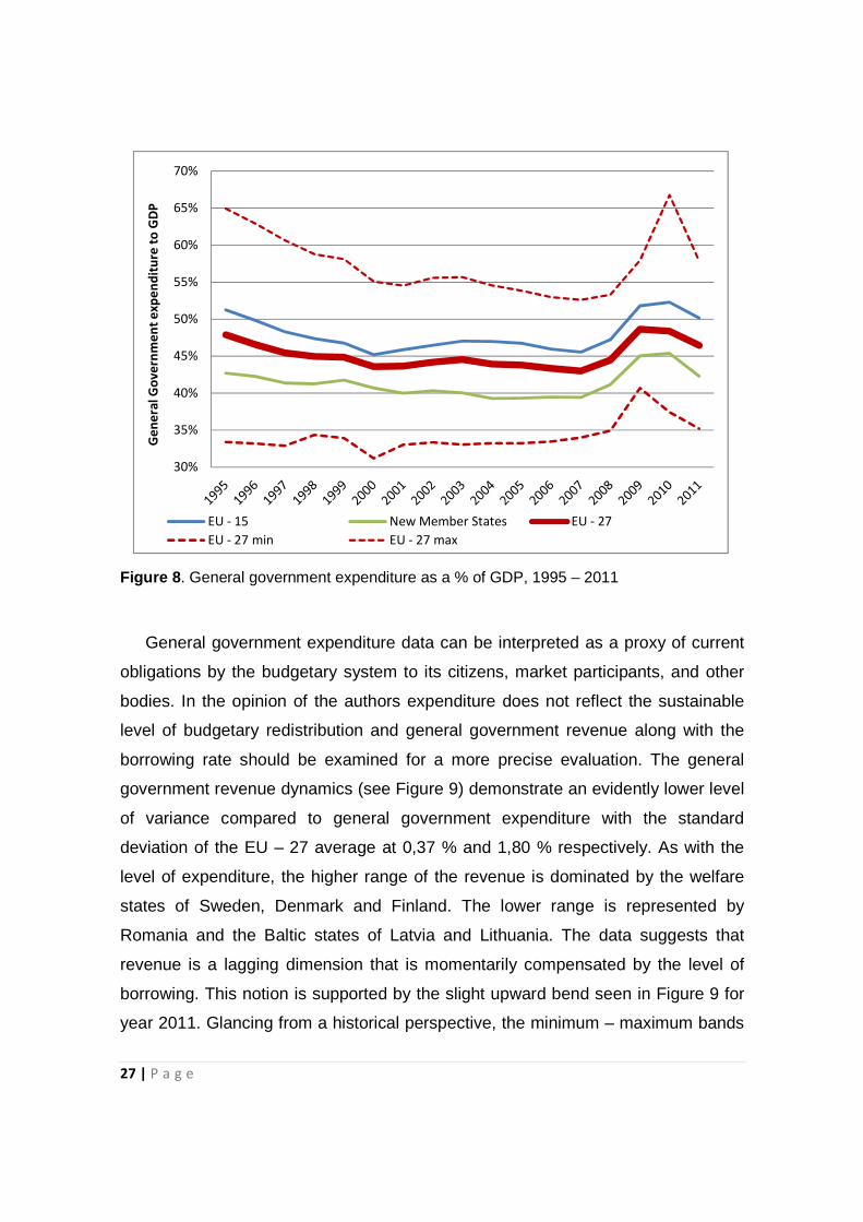
As seen in Figure 8, the dynamics of general government expenditure as a
percentage of GDP for both target groups follow a nearly identical trend with the
coefficient of correlation reaching a significant value of 0,897. The EU – 15
member states tend to have a higher level of GDP redistribution through the
budgetary system with the Scandinavian countries consistently holding the highest
levels during the sample period thus demonstrating the most typical characteristic
of welfare states. The lower range is dominated by the newest member states with
Romania, the three Baltic states and Ireland displaying the lowest redistribution
rates during the sample period; During the financial downturn Ireland moved from
the lower boundary to the highest value with an increase from 36,61 percent in
year 2007 to 66,79 percent in year 2010. The minimum and maximum bands of the
full EU – 27 sample period clearly visualizes the extreme differences of aggregate
expenditure incurred by the sectors of general government.
27 | P a g e
Figure 8. General government expenditure as a % of GDP, 1995 – 2011
General government expenditure data can be interpreted as a proxy of current
obligations by the budgetary system to its citizens, market participants, and other
bodies. In the opinion of the authors expenditure does not reflect the sustainable
level of budgetary redistribution and general government revenue along with the
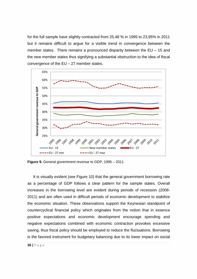
borrowing rate should be examined for a more precise evaluation. The general
government revenue dynamics (see Figure 9) demonstrate an evidently lower level
of variance compared to general government expenditure with the standard
deviation of the EU – 27 average at 0,37 % and 1,80 % respectively. As with the
level of expenditure, the higher range of the revenue is dominated by the welfare
states of Sweden, Denmark and Finland. The lower range is represented by
Romania and the Baltic states of Latvia and Lithuania. The data suggests that
revenue is a lagging dimension that is momentarily compensated by the level of
borrowing. This notion is supported by the slight upward bend seen in Figure 9 for
year 2011. Glancing from a historical perspective, the minimum – maximum bands
30%
35%
40%
45%
50%
55%
60%
65%
70%
Ge
ne
ral
Go
ve
rnm
en
t e
xp
en
dit
ure
to
GD
P
EU - 15 New Member States EU - 27
EU - 27 min EU - 27 max
28 | P a g e
for the full sample have slightly contracted from 25,48 % in 1995 to 23,95% in 2011
but it remains difficult to argue for a visible trend in convergence between the
member states. There remains a pronounced disparity between the EU – 15 and
the new member states thus signifying a substantial obstruction to the idea of fiscal
convergence of the EU – 27 member states.
Figure 9. General government revenue to GDP, 1995 – 2011
It is visually evident (see Figure 10) that the general government borrowing rate
as a percentage of GDP follows a clear pattern for the sample states. Overall
increases in the borrowing level are evident during periods of recession (2008-
2011) and are often used in difficult periods of economic development to stabilize
the economic situation. These observations support the Keynesian standpoint of
countercyclical financial policy which originates from the notion that in essence
positive expectations and economic development encourage spending and
negative expectations combined with economic contraction provokes excessive
saving, thus fiscal policy should be employed to reduce the fluctuations. Borrowing
is the favored instrument for budgetary balancing due to its lower impact on social
25%
30%
35%
40%
45%
50%
55%
60%
65%
Ge
ne
ral
go
ve
rnm
en
t re
ve
nu
e t
o G
DP
EU - 15 New member states EU - 27
EU - 27 min EU - 27 max

29 | P a g e
disorder and its immediate effect since the alternative rout of cutting budgetary
expenses and increasing the tax burden evokes immediate protests and resistance
and is not able to deliver the necessary results in a desirable time frame. However,
extensive borrowing causes certain hazards with a recent example demonstrated
by Greece and increasing distrust mounting on the EU – 15 states of Portugal,
Spain and Italy. European level discussions on fiscal austerity requirements hint on
limiting the use of borrowing for budgetary balancing.
Figure 10. General government borrowing to GDP, 1995 - 2011
Even though Maastricht criteria on the general deficit level were set out
demanded member states to limit their total government deficit to 3% of GDP as
well as limit total gross general government debt to 60% of GDP, changes were
introduced on 2nd May 2012. The new rule that is introduced in the present EU
Fiscal Compact Treaty6 allows limited temporary deviations and stipulates:
• ‘the budgetary position of the general government of a Contracting Party shall
be balanced or in surplus; 6 see Treaty on Stability, Coordination and Governance in the Economic and Monetary Union,
European Council
-10%
-5%
0%
5%
10%
15%
20%
25%
30%
35%
Ge
ne
ral
go
ve
rnm
en
t b
orr
ow
ing
to
GD
P
EU - 15 New member states EU - 27
EU - 27 min EU - 27 max
30 | P a g e
• the rule under point (a) shall be deemed to be respected if the annual structural
balance of the general government is at its country-specific medium-term
objective, as defined in the revised Stability and Growth Pact, with a lower limit
of a structural deficit of 0,5 % of the gross domestic product at market prices.
The Contracting Parties shall ensure rapid convergence towards their
respective medium-term objective. The time-frame for such convergence will
be proposed by the European Commission taking into consideration country-
specific sustainability risks. Progress towards, and respect of, the medium-term
objective shall be evaluated on the basis of an overall assessment with the
structural balance as a reference, including an analysis of expenditure net of
discretionary revenue measures, in line with the revised Stability and Growth
Pact;
• the Contracting Parties may temporarily deviate from their respective medium-
term objective or the adjustment path towards it only in exceptional
circumstances, as defined in point (b) of paragraph 3;
• where the ratio of the general government debt to gross domestic product at
market prices is significantly below 60 % and where risks in terms of long-term
sustainability of public finances are low, the lower limit of the medium-term
objective specified under point (b) can reach a structural deficit of at most 1,0
% of the gross domestic product at market prices;
• in the event of significant observed deviations from the medium-term objective
or the adjustment path towards it, a correction mechanism shall be triggered
automatically. The mechanism shall include the obligation of the Contracting
Party concerned to implement measures to correct the deviations over a
defined period of time.’
The full content of the article 3, point 1 of the aforementioned treaty was quoted
in order not to distort or restrict the purport intended by the treaty. Provisions of the
Treaty are to be employed by Contracting Parties at the latest one year after the
entry into force. On 2nd May, 2012 the treaty was signed by – thus the Contracting
Parties constitute – all members of the European Union except two: United
31 | P a g e
Kingdom and Czech Republic. The key provision of the Treaty, as noted in the
quote, is the imposed limits on the use of borrowing in the budgetary balancing
process thus putting an emphasis on fiscal austerity consisting of expenditure
cutting and revenue boosting measures.
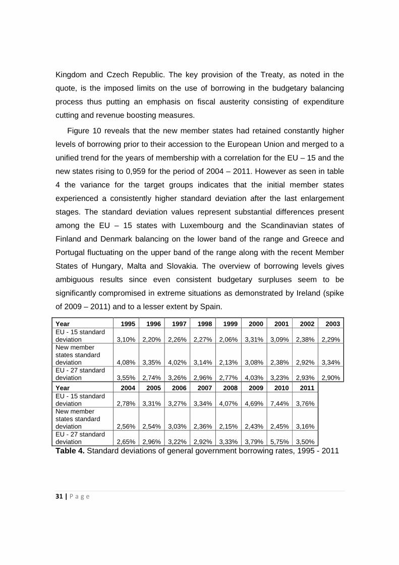
Figure 10 reveals that the new member states had retained constantly higher
levels of borrowing prior to their accession to the European Union and merged to a
unified trend for the years of membership with a correlation for the EU – 15 and the
new states rising to 0,959 for the period of 2004 – 2011. However as seen in table
4 the variance for the target groups indicates that the initial member states
experienced a consistently higher standard deviation after the last enlargement
stages. The standard deviation values represent substantial differences present
among the EU – 15 states with Luxembourg and the Scandinavian states of
Finland and Denmark balancing on the lower band of the range and Greece and
Portugal fluctuating on the upper band of the range along with the recent Member
States of Hungary, Malta and Slovakia. The overview of borrowing levels gives
ambiguous results since even consistent budgetary surpluses seem to be
significantly compromised in extreme situations as demonstrated by Ireland (spike
of 2009 – 2011) and to a lesser extent by Spain.
Year 1995 1996 1997 1998 1999 2000 2001 2002 2003 EU - 15 standard deviation 3,10% 2,20% 2,26% 2,27% 2,06% 3,31% 3,09% 2,38% 2,29% New member states standard deviation 4,08% 3,35% 4,02% 3,14% 2,13% 3,08% 2,38% 2,92% 3,34% EU - 27 standard deviation 3,55% 2,74% 3,26% 2,96% 2,77% 4,03% 3,23% 2,93% 2,90%
Year 2004 2005 2006 2007 2008 2009 2010 2011 EU - 15 standard deviation 2,78% 3,31% 3,27% 3,34% 4,07% 4,69% 7,44% 3,76% New member states standard deviation 2,56% 2,54% 3,03% 2,36% 2,15% 2,43% 2,45% 3,16% EU - 27 standard deviation 2,65% 2,96% 3,22% 2,92% 3,33% 3,79% 5,75% 3,50% Table 4. Standard deviations of general government borrowing rates, 1995 - 2011

32 | P a g e
A visualization of the debt to GDP ratios for the target groups is presented in
Figure 11. These ratios generally represent the cumulative total of the borrowing
levels throughout a certain period that have to be adjusted for the changes in GDP.
EU – 15 states tend to have a significantly higher debt to GDP ratio with a
correspondingly higher absolute standard deviation however despite the initial
differences a contraction of the range ensued with a common trend developing
afterwards. The EU – 15 and new member states have demonstrated a rather
uniform development of the debt to GDP ratio for 2004 – 2011 correlating at 0,91.
For individual countries Greece, Italy and Belgium dominate the upper range and
Luxembourg and Estonia consistently lead the lower range. An example of the
Baltic states of Latvia, Lithuania and Estonia suggest that significant differences
can exist between countries that share a common history, hold independence for a
unified period of time and are located in a relatively close proximity thus impeding
their comparability. Extreme deviations of debt to GDP and especially the growing
range pose a serious obstacle to the convergence of fiscal policies.
Figure 11. Debt to GDP ratio, 1995 – 2011
0,00
0,20
0,40
0,60
0,80
1,00
1,20
1,40
1,60
1,80
De
bt
to G
DP
ra
tip
EU - 15 New member states EU - 27 EU - 27 min EU - 27 max
33 | P a g e
3.3. Revenue composition
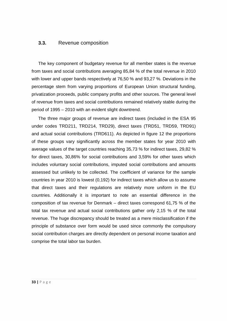
The key component of budgetary revenue for all member states is the revenue
from taxes and social contributions averaging 85,84 % of the total revenue in 2010
with lower and upper bands respectively at 76,50 % and 93,27 %. Deviations in the
percentage stem from varying proportions of European Union structural funding,
privatization proceeds, public company profits and other sources. The general level
of revenue from taxes and social contributions remained relatively stable during the
period of 1995 – 2010 with an evident slight downtrend.
The three major groups of revenue are indirect taxes (included in the ESA 95
under codes TRD211, TRD214, TRD29), direct taxes (TRD51, TRD59, TRD91)
and actual social contributions (TRD611). As depicted in figure 12 the proportions
of these groups vary significantly across the member states for year 2010 with
average values of the target countries reaching 35,73 % for indirect taxes, 29,82 %
for direct taxes, 30,86% for social contributions and 3,59% for other taxes which
includes voluntary social contributions, imputed social contributions and amounts
assessed but unlikely to be collected. The coefficient of variance for the sample
countries in year 2010 is lowest (0,192) for indirect taxes which allow us to assume
that direct taxes and their regulations are relatively more uniform in the EU
countries. Additionally it is important to note an essential difference in the
composition of tax revenue for Denmark – direct taxes correspond 61,75 % of the
total tax revenue and actual social contributions gather only 2,15 % of the total
revenue. The huge discrepancy should be treated as a mere misclassification if the
principle of substance over form would be used since commonly the compulsory
social contribution charges are directly dependent on personal income taxation and
comprise the total labor tax burden.
34 | P a g e
Figure 12. Composition of taxes and social contributions revenue as a % of GDP, 2010
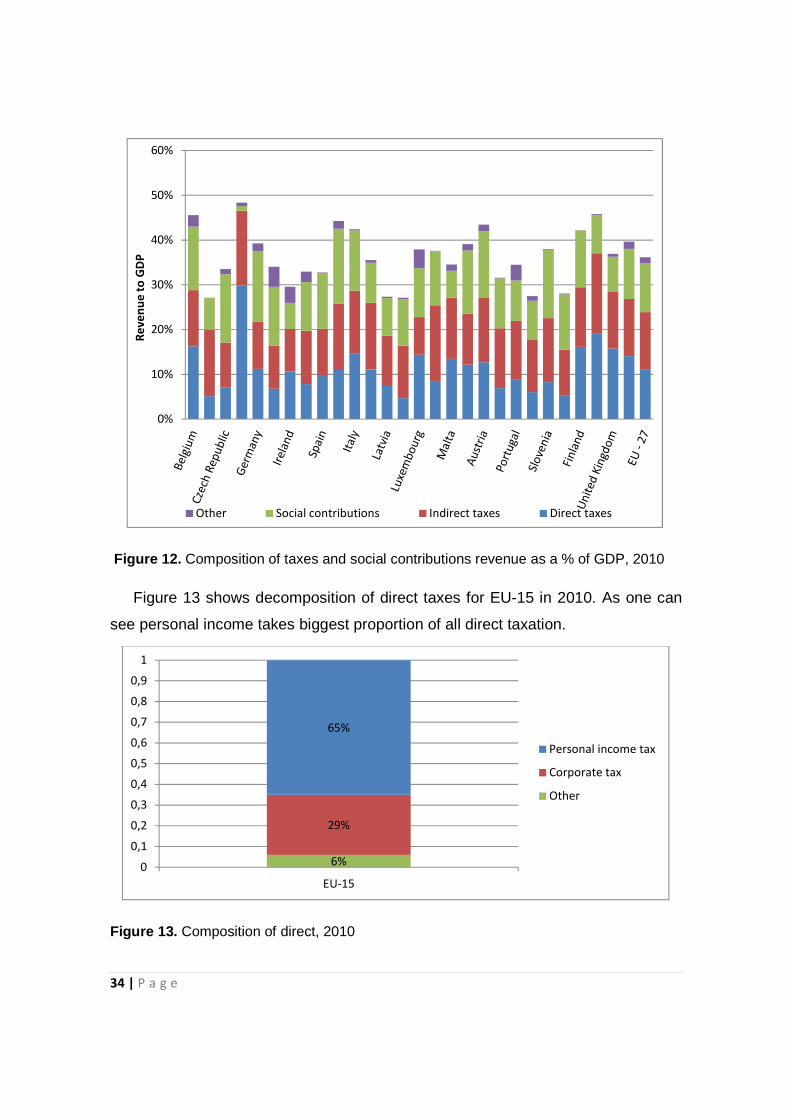
Figure 13 shows decomposition of direct taxes for EU-15 in 2010. As one can
see personal income takes biggest proportion of all direct taxation.
Figure 13. Composition of direct, 2010
0%
10%
20%
30%
40%
50%
60%R
ev
en
ue
to
GD
P
Other Social contributions Indirect taxes Direct taxes
6%
29%
65%
0
0,1
0,2
0,3
0,4
0,5
0,6
0,7
0,8
0,9
1
EU-15
Personal income tax
Corporate tax
Other

35 | P a g e
During the period of 1995 – 2010 indirect taxes with value added tax in
particular demonstrated consistent growth as the proportion of total taxes and
social contributions climbing from 18,26 % in 1995 to 21,29% in 2010 while
proceeds from income taxes saw a consistent decrease from 30,20 % in 1995 to
20,70 % in 2010. Figure 14 depicts the composition of indirect taxes for the target
groups in 2010 with the principal portion of indirect taxes comprised of value added
type taxes. The specifics of value added taxes make it an efficient tax with
relatively low administration costs. Even though the proportion and importance of
value added tax has risen during the sample period, convergence of the proceeds
for the target groups could not be identified since the gap between the groups has
slightly widened from 5,43 % to 6,23 % for 1995 - 2010, representing a 14,78 %
increase.
Figure 14. Composition of indirect taxes as a percentage of total taxes and social contributions, 2010
3.4. Income tax overview
This section depicts and analyses tax structure along with labor tax in major
observable countries. As the lack of data for labor tax revenue appears in most of
Eastern European countries and some Western European countries, this section
0
0,05
0,1
0,15
0,2
0,25
0,3
0,35
0,4
EU - 15 EU - 27
Other taxes on
products
Taxes on production
except VAT and
imports
VAT

36 | P a g e
provides tax analysis for the following 12 countries: Austria, Belgium, Denmark,
Finland, France, Germany, Italy, Netherland, Norway, Spain, Sweden, UK.
Generally, Sweden collects the highest labor tax revenue
GDP in comparison to other EU countries. UK, on the other hand, has the lowest
labor tax revenue ratio to GDP (Figure
Figure 15. Labor tax revenue as a percentage of GDP 1996
UK has the lowest implicit labor tax rate amongst EU countries. This is
illustrated in Figure 16. EU
cent in the period 1996-2010.
provides tax analysis for the following 12 countries: Austria, Belgium, Denmark,
Finland, France, Germany, Italy, Netherland, Norway, Spain, Sweden, UK.
Generally, Sweden collects the highest labor tax revenues as a proportion of
GDP in comparison to other EU countries. UK, on the other hand, has the lowest
labor tax revenue ratio to GDP (Figure 15).
Labor tax revenue as a percentage of GDP 1996-2010.
UK has the lowest implicit labor tax rate amongst EU countries. This is
. EU-27 implicit labor tax rate ranges from 35 .5 to 36.5 per
2010.
provides tax analysis for the following 12 countries: Austria, Belgium, Denmark,
Finland, France, Germany, Italy, Netherland, Norway, Spain, Sweden, UK.
s as a proportion of
GDP in comparison to other EU countries. UK, on the other hand, has the lowest
UK has the lowest implicit labor tax rate amongst EU countries. This is
27 implicit labor tax rate ranges from 35 .5 to 36.5 per

37 | P a g e
Figure 16. Implicit tax rates in EU countries 1996
Austria
Recently there is discussion weather high overall taxes in Austria downgrade
the pace of growth (Schratzenstaller, 2007). Personal income tax is progressive
and maximum marginal rate is 50%. In 2012 tax brackets for personal income tax
is illustrated in Table 5.
Income (EUR)
111,00125,00160,001 and over
Table 5. Personal income tax
Employment income is also a subject to wage tax, which is withheld by the
employer and transferred to tax authorities. Table
implicit labor tax rate dynamics for the period 1996
Implicit tax rates in EU countries 1996-2010.
Recently there is discussion weather high overall taxes in Austria downgrade
the pace of growth (Schratzenstaller, 2007). Personal income tax is progressive
and maximum marginal rate is 50%. In 2012 tax brackets for personal income tax
Income (EUR) Tax rate(%)
1-11,000 0 11,001-25,000 36.5 25,001- 60,000 43.21 60,001 and over 50
Personal income tax rates in Austria, 2011
Employment income is also a subject to wage tax, which is withheld by the
employer and transferred to tax authorities. Table 6 shows labor tax revenue and
implicit labor tax rate dynamics for the period 1996-2010. As one can see labor tax
Recently there is discussion weather high overall taxes in Austria downgrade
the pace of growth (Schratzenstaller, 2007). Personal income tax is progressive
and maximum marginal rate is 50%. In 2012 tax brackets for personal income tax
Employment income is also a subject to wage tax, which is withheld by the
shows labor tax revenue and
2010. As one can see labor tax
38 | P a g e
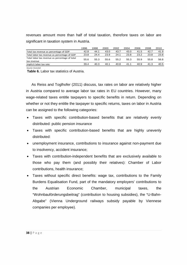
revenues amount more than half of total taxation, therefore taxes on labor are
significant in taxation system in Austria.
1996 1998 2000 2002 2004 2006 2008 2010Total tax revenue as percentage of GDP 42.8 44.1 43.0 43.7 43.0 41.5 42.7 41.9Total labor tax revenue as percentage of GDP 23.8 24.4 23.9 24.1 23.8 23.2 23.8 23.8Total labor tax revenue as percentage of total
tax revenue55.6 55.3 55.6 55.2 55.3 55.9 55.8 56.8
Implicit labor tax rate 39.4 40.3 40.1 40.8 41.1 40.9 41.3 40.5
Source: Eurostat
Table 6. Labor tax statistics of Austria.
As Reiss and Toglhofer (2011) discuss, tax rates on labor are relatively higher
in Austria compared to average labor tax rates in EU countries. However, many
wage-related taxes entitle taxpayers to specific benefits in return. Depending on
whether or not they entitle the taxpayer to specific returns, taxes on labor in Austria
can be assigned to the following categories:
• Taxes with specific contribution-based benefits that are relatively evenly
distributed: public pension insurance
• Taxes with specific contribution-based benefits that are highly unevenly
distributed:
• unemployment insurance, contributions to insurance against non-payment due
to insolvency, accident insurance;
• Taxes with contribution-independent benefits that are exclusively available to
those who pay them (and possibly their relatives): Chamber of Labor
contributions, health insurance;
• Taxes without specific direct benefits: wage tax, contributions to the Family
Burdens Equalisation Fund, part of the mandatory employers’ contributions to
the Austrian Economic Chamber, municipal taxes, the
“Wohnbauförderungsbeitrag” (contribution to housing subsidies), the “U-Bahn-
Abgabe” (Vienna Underground railways subsidy payable by Viennese
companies per employee).

39 | P a g e
Belgium
Belgium has progressive personal income tax system. Table 7 depicts tax
brackets for different income.
Income (EUR) Tax rate (%)
1-7,900 25 7,901-11,240 30 11,241- 18,730 40 18,731-34,330 45 34,331 and over 50
Table 7. Personal income tax rates in Belgium, 2011
Also there is additional tax-free allowance for dependent children: EUR 1,370
for one child, EUR 3,520 for two children and EUR 7,889 for three and more
children. As for labor taxes, an implicit labor tax in Belgium varies from 42.4 per
cent to 44 percent in the period 1996-2010. Labor tax revenues account for more
than 50 per cent of total taxation. This is illustrated in Table 8.
1996 1998 2000 2002 2004 2006 2008 2010Total tax revenue as percentage of GDP 44.4 45.5 45.1 45.2 44.9 44.4 44.3 44.0Total labor tax revenue as percentage of GDP 24.2 24.5 24.2 24.8 24.0 23.0 23.6 23.8Total labor tax revenue as percentage of total
tax revenue54.5 53.9 53.7 54.9 53.5 51.8 53.3 54.1
Implicit labor tax rate 43.2 44.0 43.6 43.3 43.8 42.5 42.4 42.5
Source: Eurostat
Table 8. Labor tax statistics of Belgium.
Denmark
Taxable income in Denmark is taxed at progressive rates up to 51.5 per cent.
The municipal taxes are determined by each county and range from 22.8 per cent
to 27.8 per cent; the health tax is 8 per cent and the church tax, which is optional,
ranges from 0.44 per cent to 1.5 per cent. The state tax consists of a bottom
bracket tax of 3.76 per cent, and a top bracket tax of 15 per cent for income
exceeding DKK 389,900. A special 25 per cent (or 33 per cent) taxation scheme

40 | P a g e
may be available for approved scientists or employees/individuals that meet the
high salary qualification.
In Table 9 one can see implicit labor tax rate decrease starting 2004. This can
be partly explained by tax cut introduced in 2004 (Eurostat, 2007).
1996 1998 2000 2002 2004 2006 2008 2010Total tax revenue as percentage of GDP 49.2 49.3 49.4 47.9 49.0 49.6 47.7 47.6Total labor tax revenue as percentage of GDP 27.3 26.3 26.6 26.1 25.2 24.6 25.4 24.6Total labor tax revenue as percentage of total
tax revenue55.5 53.3 53.9 54.5 51.4 49.6 53.3 51.7
Implicit labor tax rate 40.2 38.9 41.0 38.8 37.5 36.9 36.6 34.8
Source: Eurostat
Table 9. Labor tax statistics of Denmark.
Another tax reform was implemented recently. On 1 March 2009 the Danish
government formed a political agreement with Dansk Folkeparti (The Danish
Peoples Party) on a tax reform from 2010 – the so called Forårspakke 2.0. The
legislation was adopted by parliament by the end of May 2009 and will gradually
come into force during the years 2010-2019. The reform involves tax cuts and
financing of around 30 billion DKK corresponding to around 1.5% of GDP (The
Danish Ministry of Taxation, 2009).
Finland
Taxes on personal income are progressive and are shown in Table 10.
Additionally, municipal income tax must be added, which varies from 16.5 per cent
to 21 per cent.
Taxable income (EUR)
Tax on lower amount (EUR)
Rate on excess (%)
15,200 – 22,600 8 8.5
22,601 – 36,800 489 17.5 36,801 – 66,400 2,974 21.5 66,401 and over 9,338 30.0
Table 10. Personal income tax rates in Finland, 2011
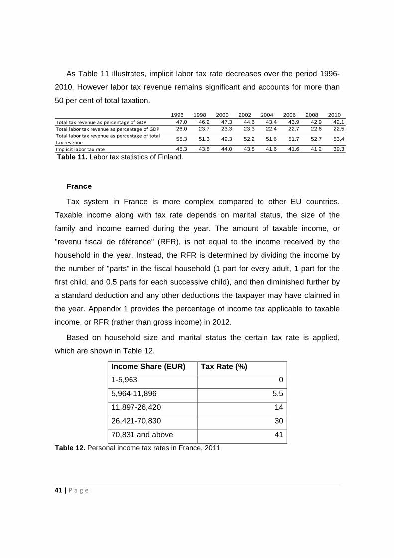
41 | P a g e
As Table 11 illustrates, implicit labor tax rate decreases over the period 1996-
2010. However labor tax revenue remains significant and accounts for more than
50 per cent of total taxation.
1996 1998 2000 2002 2004 2006 2008 2010Total tax revenue as percentage of GDP 47.0 46.2 47.3 44.6 43.4 43.9 42.9 42.1Total labor tax revenue as percentage of GDP 26.0 23.7 23.3 23.3 22.4 22.7 22.6 22.5Total labor tax revenue as percentage of total
tax revenue55.3 51.3 49.3 52.2 51.6 51.7 52.7 53.4
Implicit labor tax rate 45.3 43.8 44.0 43.8 41.6 41.6 41.2 39.3
Table 11. Labor tax statistics of Finland.
France
Tax system in France is more complex compared to other EU countries.
Taxable income along with tax rate depends on marital status, the size of the
family and income earned during the year. The amount of taxable income, or
"revenu fiscal de référence" (RFR), is not equal to the income received by the
household in the year. Instead, the RFR is determined by dividing the income by
the number of "parts" in the fiscal household (1 part for every adult, 1 part for the
first child, and 0.5 parts for each successive child), and then diminished further by
a standard deduction and any other deductions the taxpayer may have claimed in
the year. Appendix 1 provides the percentage of income tax applicable to taxable
income, or RFR (rather than gross income) in 2012.
Based on household size and marital status the certain tax rate is applied,
which are shown in Table 12.
Income Share (EUR) Tax Rate (%)
1-5,963 0
5,964-11,896 5.5
11,897-26,420 14
26,421-70,830 30
70,831 and above 41
Table 12. Personal income tax rates in France, 2011

42 | P a g e
Labor tax rate during the period 1996-2010 fluctuates at the tight range 41.0-
42.1 per cent (Table 13).
1996 1998 2000 2002 2004 2006 2008 2010Total tax revenue as percentage of GDP 44.1 44.1 44.2 43.3 43.3 44.1 43.3 42.5Total labor tax revenue as percentage of GDP 23.0 22.8 23.0 22.8 22.9 23.0 22.8 23.1Total labor tax revenue as percentage of total
tax revenue52.2 51.7 52.0 52.7 52.9 52.1 52.7 54.3
Implicit labor tax rate 41.4 42.1 41.9 41.1 41.3 41.7 41.5 41.0
Source: Eurostat
Table 13. Labor tax statistics of France.
Germany
In 2000 Germany has performed tax reform, which is considered to be the most
ambitious tax reform in postwar German history (Haan and Steiner, 2005). Since
the tax reform was complex, basically personal tax rates were raised, but tax base
were narrowed.
Although a slight decrease of implicit labor tax rate is observed since 2000,
labor tax revenue in Germany still constitutes large share of all tax revenues
collected (Table 13).
1996 1998 2000 2002 2004 2006 2008 2010Total tax revenue as percentage of GDP 40.1 40.4 41.2 38.9 38.3 38.6 38.8 38.1Total labor tax revenue as percentage of GDP 23.9 24.0 24.0 23.6 22.7 21.7 21.5 21.4Total labor tax revenue as percentage of total
tax revenue59.6 59.4 58.2 60.7 59.3 56.2 55.4 56.2
Implicit labor tax rate 38.3 39.2 39.1 38.7 37.8 37.6 38.0 37.4
Source: Eurostat
Table 13. Labor tax statistics of Germany.
Italy
Italy has progressive tax system. Personal income tax is applied depending on
income level. Table 14 depicts different personal income tax rates.

43 | P a g e
Taxable Income
(EUR)
Tax Rate (%)
Up to 15,000 23
15,001 – 28,000 27
28,001 – 55,000 38
55,001 – 75,000 41
Over 75,000 43
Table 14. Personal income tax rates in Italy, 2011
The share of labor tax increased during the period 1996-2010. In 2010 labor tax
revenue was 51.6 per cent of total tax revenue, while implicit labor tax rate jumped
to 42.6 per cent (Table 15).
1996 1998 2000 2002 2004 2006 2008 2010Total tax revenue as percentage of GDP 41.7 42.3 41.5 40.4 40.3 41.8 42.7 42.2Total labor tax revenue as percentage of GDP 19.8 20.7 19.7 20.0 20.0 20.3 21.5 21.8Total labor tax revenue as percentage of total
tax revenue47.5 48.9 47.5 49.5 49.6 48.6 50.4 51.6
Implicit labor tax rate 41.5 43.1 41.8 41.8 41.5 40.8 42.8 42.6
Source: Eurostat
Table 15. Labor tax statistics of Italy.
Netherlands
The Netherlands has a system of personal income tax known as the 'box
system'. The boxes contain three different types of income. Taxable income is
divided as follows:
• Box 1: Taxable income from work and home (only the main residence);
• Box 2: Taxable income from substantial interests in companies with limited
liability;
• Box 3: Income from savings and investment.
As for box 1, tax rate is progressive to 52 per cent (Table 16).
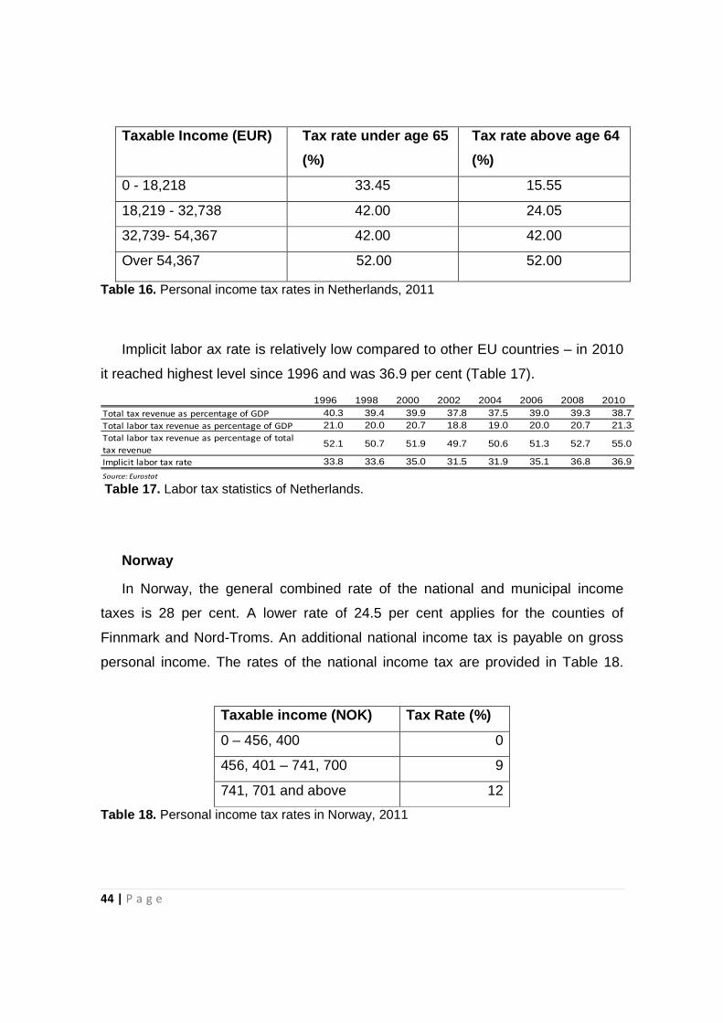
44 | P a g e
Taxable Income (EUR) Tax rate under age 65
(%)
Tax rate above age 64
(%)
0 - 18,218 33.45 15.55
18,219 - 32,738 42.00 24.05
32,739- 54,367 42.00 42.00
Over 54,367 52.00 52.00
Table 16. Personal income tax rates in Netherlands, 2011
Implicit labor ax rate is relatively low compared to other EU countries – in 2010
it reached highest level since 1996 and was 36.9 per cent (Table 17).
1996 1998 2000 2002 2004 2006 2008 2010Total tax revenue as percentage of GDP 40.3 39.4 39.9 37.8 37.5 39.0 39.3 38.7Total labor tax revenue as percentage of GDP 21.0 20.0 20.7 18.8 19.0 20.0 20.7 21.3Total labor tax revenue as percentage of total
tax revenue52.1 50.7 51.9 49.7 50.6 51.3 52.7 55.0
Implicit labor tax rate 33.8 33.6 35.0 31.5 31.9 35.1 36.8 36.9
Source: Eurostat
Table 17. Labor tax statistics of Netherlands.
Norway
In Norway, the general combined rate of the national and municipal income
taxes is 28 per cent. A lower rate of 24.5 per cent applies for the counties of
Finnmark and Nord-Troms. An additional national income tax is payable on gross
personal income. The rates of the national income tax are provided in Table 18.
Taxable income (NOK) Tax Rate (%)
0 – 456, 400 0
456, 401 – 741, 700 9
741, 701 and above 12
Table 18. Personal income tax rates in Norway, 2011

45 | P a g e
A personal allowance of NOK 84,420 is available to jointly assessed married
couples and for single persons with dependents. The allowance for single persons
without dependents and married persons assessed separately is NOK 42,210).
In addition, social security taxes are paid. Employees pay 7.8 per cent of gross
salary income. For self-employed individuals the rate is 11 per cent.
Table 19 shows that implicit labor tax in Norway is lower compared to other EU
countries. Also labor tax revenue makes only 36.8-42.9 percent of total tax revenue
(range for the period 1996-2010). This shows that labor tax is not so important as it
is in other EU countries, still it remains significant in total tax composition.
1996 1998 2000 2002 2004 2006 2008 2010Total tax revenue as percentage of GDP 42.4 42.0 42.6 43.1 43.1 43.5 42.1 42.9Total labor tax revenue as percentage of GDP 18.2 19.9 17.2 18.6 17.8 16.0 16.2 17.8Total labor tax revenue as percentage of total
tax revenue42.9 47.4 40.4 43.2 41.3 36.8 38.5 41.5
Implicit labor tax rate 37.0 37.3 37.1 37.5 37.8 36.6 35.8 36.1
Source: Eurostat
Table 19. Labor tax statistics of Norway.
Spain
Personal income tax rates in Spain are progressive to 43 per cent. Detailed tax
rates are shown in Table 20.
Income (EUR) Tax Rate (%)
0 - 17,707 24
17,707 - 33,007 28
33,007 - 53,407 37
53,407 and more 43
Table 20. Personal income tax rates in Spain, 2011
When the earned income is less than EUR 22,000, the individual is not obliged to
prepare a tax return. If there is more than one individual in the same family unit, the
limit is EUR 8,000. Although personal income tax is progressive, Spain has many
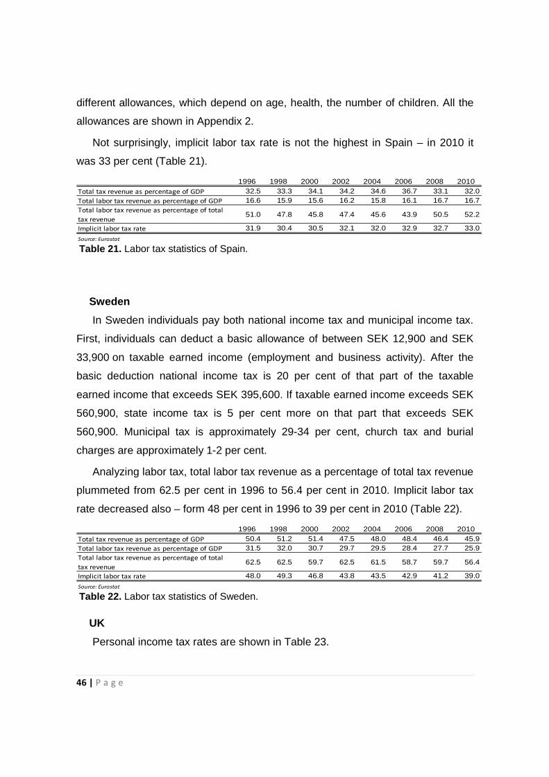
46 | P a g e
different allowances, which depend on age, health, the number of children. All the
allowances are shown in Appendix 2.
Not surprisingly, implicit labor tax rate is not the highest in Spain – in 2010 it
was 33 per cent (Table 21).
1996 1998 2000 2002 2004 2006 2008 2010Total tax revenue as percentage of GDP 32.5 33.3 34.1 34.2 34.6 36.7 33.1 32.0Total labor tax revenue as percentage of GDP 16.6 15.9 15.6 16.2 15.8 16.1 16.7 16.7Total labor tax revenue as percentage of total
tax revenue51.0 47.8 45.8 47.4 45.6 43.9 50.5 52.2
Implicit labor tax rate 31.9 30.4 30.5 32.1 32.0 32.9 32.7 33.0
Source: Eurostat
Table 21. Labor tax statistics of Spain.
Sweden
In Sweden individuals pay both national income tax and municipal income tax.
First, individuals can deduct a basic allowance of between SEK 12,900 and SEK
33,900 on taxable earned income (employment and business activity). After the
basic deduction national income tax is 20 per cent of that part of the taxable
earned income that exceeds SEK 395,600. If taxable earned income exceeds SEK
560,900, state income tax is 5 per cent more on that part that exceeds SEK
560,900. Municipal tax is approximately 29-34 per cent, church tax and burial
charges are approximately 1-2 per cent.
Analyzing labor tax, total labor tax revenue as a percentage of total tax revenue
plummeted from 62.5 per cent in 1996 to 56.4 per cent in 2010. Implicit labor tax
rate decreased also – form 48 per cent in 1996 to 39 per cent in 2010 (Table 22).
1996 1998 2000 2002 2004 2006 2008 2010Total tax revenue as percentage of GDP 50.4 51.2 51.4 47.5 48.0 48.4 46.4 45.9Total labor tax revenue as percentage of GDP 31.5 32.0 30.7 29.7 29.5 28.4 27.7 25.9Total labor tax revenue as percentage of total
tax revenue62.5 62.5 59.7 62.5 61.5 58.7 59.7 56.4
Implicit labor tax rate 48.0 49.3 46.8 43.8 43.5 42.9 41.2 39.0
Source: Eurostat
Table 22. Labor tax statistics of Sweden.
UK
Personal income tax rates are shown in Table 23.

47 | P a g e
Income (GBP) Tax Rate (%)
0 – 37,400 20
37,401 – 150,000 40
Over 150,000 50
Table 23. Personal income tax rates in UK, 2011
United Kingdom has the lowest implicit labor tax rate amongst all observable
countries. Implicit labor tax rate was 25.7 per cent in 2010. Total tax revenue as a
percentage of GDP is the lowest as well. In 2010 more than 40 per cent of total tax
revenue was collected from labor tax (Table 24).
1996 1998 2000 2002 2004 2006 2008 2010Total tax revenue as percentage of GDP 34.4 36.0 36.7 34.9 35.2 36.7 38.0 35.6Total labor tax revenue as percentage of GDP 13.1 13.6 14.3 13.7 13.9 14.4 14.7 14.3Total labor tax revenue as percentage of total
tax revenue38.1 37.8 39.0 39.2 39.5 39.2 38.7 40.2
Implicit labor tax rate 25.0 25.3 25.9 24.7 25.5 26.5 26.9 25.7
Source: Eurostat
Table 23. Labor tax statistics of UK.
3.5. VAT overview
Value added tax in European Union is applied in a relatively uniform manner.
The common system of VAT applies to the production and distribution of goods
and services bought and sold for consumption within the European Union and the
actual tax burden are visible at each stage in the production and distribution. VAT
is finally borne by the final consumer in the form of a percentage addition to the
final price of the goods or services (The European e-Justice Portal under the
European Commission). The application of Value added tax was regulated by the
Sixth Directive up to 1 January 2007 and by the VAT Directive onwards. The VAT
Directive does not set out specific rates to be applied in the member states, the
main requirement is for the minimum value of the standard rate of 15 %; the
Directive also allows Member States many possible exceptions and derogations
from the standard VAT coverage. The VAT system is currently in a transitional
mode as a destination based system with the intention of transforming to an origin

48 | P a g e
based system thus changes in the future are inevitable. The major source of
variation between member states are the tax rates including reduced rates and
zero rating, and exemptions that follow individualized provisions, i.e. the minimum
registration threshold for small enterprises.
VAT revenue has demonstrated a consistent increase as a percentage of GDP
during the period of 1995 – 2010 (Figure 15). The higher band of the range is
mainly populated by the new member states like Bulgaria, Estonia and Lithuania
and the lower band of the range by Italy, Luxembourg and Belgium. Despite the
uniformity of VAT regulations, the proportion of revenue to GDP remains highly
scattered. The significant differences are induced by varying levels of zero-
rating and exemptions as individual countries are free to determine VAT
thresholds. The thresholds range from 5580 EUR in Belgium to 81843 EUR in
United Kingdom with the absolute majority of member states clustering around the
lower part of the range. Controversially the new member states are generally
exhibiting higher threshold limits than the EU – 15 states (Appendix 3).
Figure 15. VAT revenue as a percentage to GDP, 1995 - 2010
5%
10%
15%
20%
25%
30%
35%
40%
VA
T r
ev
en
ue
to
GD
P
EU - 15 New member states EU - 27 EU - 27 min EU - 27 max

49 | P a g e
Standard VAT rates have also demonstrated a consistent rise throughout the
sample period with an especially sharp increase in years 2009 and 2010 (Figure
16). This sharp rise indicates that value added taxes might be used as a primary
line for budgetary revenue balancing and might be used to offset the possible
limitations of borrowing accessibility. Empirical data implies that VAT rates have
grown strongly as a result of the crisis. VAT standard rates have often changed
from 2009 onwards, in the vast majority of cases upwards with an impressive
relative 3,73 % increase for 2008 – 2010. The amazing aspect of this development
is the rapid spread of VAT rate increases throughout the Union. While in 2008 only
Portugal changed the standard VAT rate, six did in 2009 and another eight
countries increased their rates in 2010, among which Greece by four points and
Romania by five. During the last 5 years only United Kingdom employed a VAT
rate cut of 2,5% in 1 December of 2008 but abandoned it in 1 January 2010
additionally announcing a rate hike of 2,5% in 4 January 2011.
Figure 16. Average VAT rates in EU – 27 for 1995 – 2010.
The period of value added tax employment in the European Union member
states saw a total of 120 changes in the standard tax rate (European Commission
VAT report, 2012). In a majority of cases the standard tax rate was increased (92)
with only 28 reported instances attributed to a VAT cut, 9 of the cuts were
18,4%
18,6%
18,8%
19,0%
19,2%
19,4%
19,6%
19,8%
20,0%
20,2%
20,4%
Av
era
ge
VA
T r
ate
s
50 | P a g e
employed by Ireland and France – member states with the most changes
performed. According to the report, eight countries applied a zero rate in
consumption. The most dominating sectors of zero-rating are the sales of
newspapers and/or other printed materials (Belgium, Denmark, Ireland, Sweden,
United Kingdom, Finland), medicine (Ireland, Malta, Sweden, United Kingdom) and
consumption associated with the agricultural sector (Ireland, Malta, United
Kingdom) and other. United Kingdom and Ireland offered a widest coverage of zero
rated consumption; however the exact value of actual zero-rated consumption
cannot be supplied due to the confidentiality of data.
Regarding the sample countries reduced rates are used extensively and in
varying proportions with five states – Spain, France, Ireland, Italy and Luxembourg
using super reduced rates for certain fields of consumption. The rate itself varied
significantly in the range of 2,1 % to 4,8% and huge deviations in the super
reduced rate coverage applied across the countries was evident with food
products, printables (especially periodicals and newspapers) and construction
sector being the primary beneficiaries of the rate. Luxembourg enjoyed the widest
coverage of super reduced rates and Ireland employed the rate only for food
products.
VAT revenue ratio is a universal indicator compounding the effects of reduced,
super reduced and zero rates, VAT exemption and VAT evasion. The VAT revenue
ratio consists of actual VAT revenues collected divided by the product of the VAT
standard rate and net final consumption, i.e. final consumption expenditure minus
VAT receipts. In essence the ratio represents the proportion of the theoretical
(calculated on the assumption that all consumption would be taxed at the standard
rate and consumption would not react to the change in VAT burden) and actual
VAT revenue.
A low value of the ratio suggests that exemptions, reduced rates, or tax evasion
have a significant impact on revenue collection. The final consumption expenditure
(P3 in ESA 95) includes the household final consumption expenditure (private
consumption), non-profit institutions serving households (NPISH) final consumption
expenditure and general government final consumption expenditure. The indicator
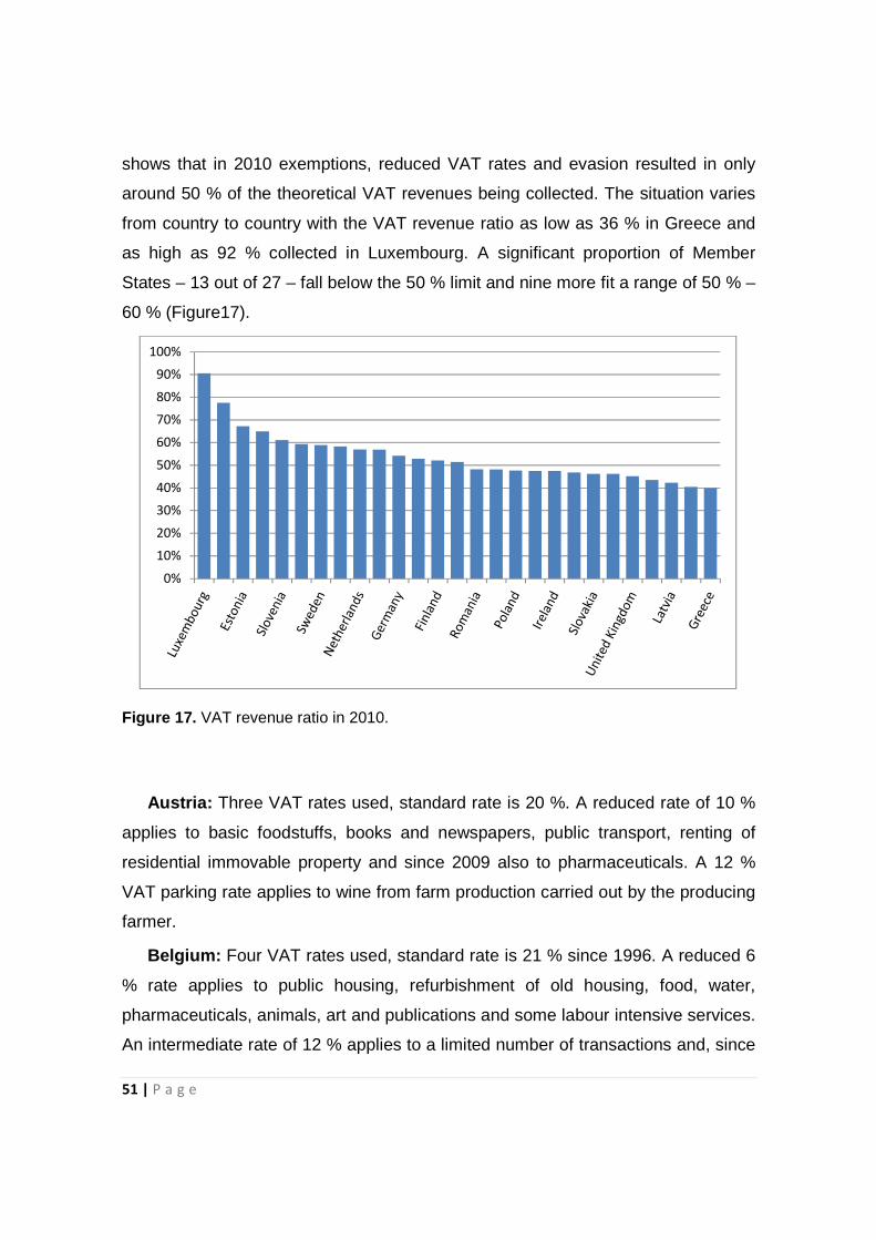
51 | P a g e
shows that in 2010 exemptions, reduced VAT rates and evasion resulted in only
around 50 % of the theoretical VAT revenues being collected. The situation varies
from country to country with the VAT revenue ratio as low as 36 % in Greece and
as high as 92 % collected in Luxembourg. A significant proportion of Member
States – 13 out of 27 – fall below the 50 % limit and nine more fit a range of 50 % –
60 % (Figure17).
Figure 17. VAT revenue ratio in 2010.
Austria: Three VAT rates used, standard rate is 20 %. A reduced rate of 10 %
applies to basic foodstuffs, books and newspapers, public transport, renting of
residential immovable property and since 2009 also to pharmaceuticals. A 12 %
VAT parking rate applies to wine from farm production carried out by the producing
farmer.
Belgium: Four VAT rates used, standard rate is 21 % since 1996. A reduced 6
% rate applies to public housing, refurbishment of old housing, food, water,
pharmaceuticals, animals, art and publications and some labour intensive services.
An intermediate rate of 12 % applies to a limited number of transactions and, since
0%
10%
20%
30%
40%
50%
60%
70%
80%
90%
100%
52 | P a g e
1st January 2010, to food in restaurants and catering services. A zero rate applies
to newspapers and certain weeklies.
Bulgaria: Two VAT rates used, standard rate is 20 %. The reduced rate of 9 %
applies to hotel accommodation and was increased from 7 % in April 2011.
Cyprus: Four VAT rates used, standard rate is 15 %. Reduced rates of 5 %
and 8 % are used for foodstuff and pharmaceutical products,
construction/purchase of the first residence, accommodation and restaurant
services, etc. Zero rate is applied on supplies of goods and services to sea-going
vessels, and international transportation, as well as exports and intra-Community
dispatches of goods and services In addition Cyprus exempts certain products –
letting of immovable property, cultural, sport, banking, insurance, medical and
hospital services.
Czech Republic: Two VAT rates used, standard rate is 20 %.Reduced rate of
14 % applies to food products, pharmaceuticals products as well as to some
services. Certain services (e.g. postal, broadcasting, banking, insurance, financial,
health and social welfare, transfer and lease of land and buildings or structures,
provision of lotteries and similar games of chance and education) are exempted
without credit for input tax.
Denmark: Two VAT rates used, standard rate is 25 %. Zero rate applied to
newspapers.
Estonia: Two VAT rates used, standard rate is 20 %. A 9 % reduced rate
applies to a limited list of goods (books, periodicals, medicine, accommodation).
Finland: Three VAT rates used, standard rate is 23%.The reduced rate of 13 %
is applied on selected goods and services, including food and restaurants.
Reduced rate of 9 % is applied on hotels, medicines, books and tickets to cultural
events, newspapers etc.
France: Four VAT rates used, standard rate is 19.6 %. Reduced rates of 5,5 %
is applied to essential goods and 7 % to the housing sector, accommodation and
restaurant services. Additionally a super reduced rate of 2.1 % applies to
newspapers, theatre performances and approved medicines.

53 | P a g e
Germany: Two VAT rates used, standard rate is 19 %. A 7 % reduced VAT
rate is applied to certain products, e.g. for staple food, public transport and books,
hotels and pensions. Few exemptions are also granted (rents and doctors'
services).
Greece: Three VAT rates used, standard rate is 23%. A reduced rate of 13 % is
applied to goods such as fresh food products, some pharmaceuticals,
transportation and electricity, certain professional services, and services by doctors
and dentists. A 6.5 % rate applies to hotel accommodation services, newspapers,
periodicals and books. For the regions of the Dodecanese, the Cyclades and
Eastern Aegean islands the above rates are reduced by 30 %.
Hungary: Three VAT rates used, standard rate is 27%.A reduced rate of 18%
is applied to while milk, milk products, bread, bakery products, and accommodation
services. 5 % is applied to district heating services, specific medicines and medical
materials, books, newspapers, etc.
Ireland: Four VAT rates used, standard rate is 21 %. The reduced rates of 13.5
% applies to various services, newspapers, building work and household energy
and fuels and 9% applies to hotel services. A zero rate applies to basic food,
children's clothing, children's footwear and books along with Exemptions on
transport services.
Italy: Three VAT rates used, standard rate is 21%. A reduced rate of 10 %
applies to non-luxury housing, other foodstuffs, electricity, mineral oil, medicines
and artistic performances. The super-reduced rate applies mostly to staple
foodstuffs, newspapers, some medical appliances, and residential housing.
Latvia: Two VAT rates used, standard rate is 22%. The reduced rate of 12 % is
applicable on: supplies of medicines, medical devices and medical goods,
specialized products intended for infants, the inland public transport services,
supply of heating to households and guest accommodation services.
Lithuania: Three VAT rates used, standard rate is 21%. The temporary
reduced rate of 9 % applies to books and non-periodical publications, residential
heating and the 5 % rate is applicable to medicines.

54 | P a g e
Luxembourg: Six VAT rates used, standard rate is 15 %. A reduced rate of 6
% applies to gas, electric power, flowers and labor-intensive services such as
hairdressing and window cleaning. An intermediary rate of 12 % applies to wine
and coal. Rates of 4 % or 10 % apply to farmers and foresters subject to a specific
regime. A super-reduced rate of 3 % applies to food and beverages,
pharmaceutical products, books and newspapers and passenger transport.
Malta: Four VAT rates used, standard rate is 18 %. A 7 % reduced rate is
applied to holiday accommodation, 5 % rate applies to letting of sites for artistic or
cultural activities, electricity, printed material, medical accessories and goods
intended for the use of disabled persons. Zero-rated supplies include food,
pharmaceutical goods, local transport and cultural services.
Netherlands: Two VAT rates used, standard rate is 19 %. The reduced rate of
6 % applies to inter alia, food, water, pharmaceuticals, art, cultural events and
publications.
Poland: Four VAT rates used, standard rate is 23 %. The reduced rates of5 %
and 8 % applies to certain foodstuffs, children’s footwear, domestic transport,
social housing, etc. Zero rate is used of international transport, etc.
Portugal: Four VAT rates used, standard rate is 23 %. The 6 % reduced rate is
applied to domestic transport services, construction, agricultural inputs, etc. The 13
% rate is applied to catering services, and zero rate is applied to international
transportation.
Romania: Four VAT rates used, standard rate is 24 %. A reduced rate of 9 %
applies to goods such as pharmaceutical products, medical equipment for disabled
persons, books, newspapers, admission to cultural services and hotel
accommodation. A 5 % reduced rate applies to the supply of social and some
private dwellings. VAT exemptions without right of deduction apply to, among
others, medical treatments, some educational and cultural activities, public postal
services, certain banking and financial transactions, insurance and reinsurance.
Slovakia: Three VAT rates used, standard rate is 20 %. The 10 % reduced rate
is applicable to medicines, certain other medical and pharmaceutical products to
55 | P a g e
books. Zero rate applies to intra-Community supply of goods, export of goods,
provision of services consisting of work on movable assets returned to a third
country, transport services and passenger transport, and services directly related
to import and export of goods.
Slovenia: Two VAT rates used, standard rate is 20 %. The reduced rate of 8.5
% applies to supply of goods and services including, inter alia, books, food,
agricultural and pharmaceutical products, certain services provided at the local
level.
Spain: Three VAT rates used, standard rate is 18 %. The 8 % rate applies to
specific categories of goods like catering, domestic and international
transportation, agricultural inputs and others. The super reduced rate of 4 %
applies to some foodstuffs, books, newspapers and other periodicals,
pharmaceuticals and construction services.
Sweden: Four VAT rates used, standard rate is 25 %. A reduced rate of 12 %
applies to foodstuffs and to services related to tourism, restaurants and catering. A
reduced rate of 6 % applies to domestic daily and weekly newspapers and
periodicals; domestic transportation of persons and ski-lift services; cinema, circus
and concert admission fees. A zero rate is applied to prescription medicines, gold
for investment purposes, and a number of financial services as well as insurance
and reinsurance services. Some sectors are exempt from the tax altogether, like
the purchase and rental of immovable property; medical, dental and social care;
education, banking and other financial services, certain cultural and sporting
activities.
United Kingdom: Three VAT rates used, standard rate is 20 %. A reduced rate
of 5 % applies, for example to fuel and power and also on the installation of energy
saving materials. A zero-rate is used extensively as it applies to some food items,
books, new constructions, passenger transport, some supplies to charities and to
children's clothing and footwear. Some exemptions also apply.
56 | P a g e
4. LABOR TAX REVENUE ESTIMATION
4.1. Labor tax ratio determination
Tax rate on labor usually is not unique in single country. EU countries have
complex tax system and most of the countries have several income tax rates
depending on tax base brackets or even marital status. For example, in the UK
there are three different income tax rates: 20 per cent, if person's taxable income is
under £35 500; 40 per cent if taxable income is in the range of £35 001 - £150 000;
50 per cent if taxable income is over £150 000. In Ireland tax brackets varies for
married taxpayers and single ones - threshold for single taxpayers is 32 800 €, for
married taxpayers – 41 800 €. Because of such complexity and other tax
exemptions and deductions, we cannot apply weighted tax rate method.
In many academic studies tax revenues are expressed as a ratio of some
aggregate tax base. Such ratios are often called as average tax ratios, or as
implicit tax rates. The discussion and research of implicit tax rates started with the
paper of Mendoza, Razin, & Tesar (1994). They suggested using average effective
tax rate, which is easy to compute. Using Mendoza et al. (1994) methodology, it is
possible to calculate indicators of the tax burden on, for example, consumption,
labor, capital and corporate income. Mendoza, Razin, & Tesar (1994) distinguished
following five different tax ratios: a personal income tax ratio, a labor income tax
ratio, a capital income tax ratio, a corporate income tax ratio and a consumption
tax ratio. Later Mendoza, Milesi-Ferretti, & Asea (1997) updated data of previous
study. Jarass & Obermair (1997) also came up with a “natural resources &
environment” tax ratio. OECD Revenue Statistics report compares tax ratios
among different countries by expressing the aggregate revenue of one particular
tax as a percentage of GDP. Other method to measure differences among tax
systems is to compare the impact of statutory tax rates, calculated for individual
taxpayers. The example can be found in the OECD publication The Tax/Benefit
Position of Employees (OECD 1998b).
57 | P a g e
In this paper, the methodology of Mendoza et al. (1997) is chosen to calculate
tax rate on labor. Volkerink and de Haan (2001) points out the following
advantages of average effective tax ratios:
• Effective tax ratios are much simpler to calculate than marginal effective tax
rates, where one has to take into account all kinds of deductions and reliefs
that are probably not very representative anyway.
• Effective tax ratios are much easier to compare by country because they are in
most cases constructed in a similar way for each country.
• Effective tax ratios are an appropriate input for macroeconomic models
• Effective tax ratios indicate real changes in the tax system that might be over-
or understated by, for example, a tax-to-GDP ratio.
In order to calculate the average effective tax ratio on labor (τl), it is necessary
to calculate the average effective tax ratio on total household income, τh. Average
effective tax ratio on total household income allocates personal income tax to
capital and labor under the assumption that the average tax rate paid on each is
the same. τh is calculated as follows:
τh = 1100/(OSPUE+PEI + W) (1)
Where7
1100 – Tax revenue on income, profits, and capital gains on individuals,
OSPUE - Operating surplus of private unincorporated enterprises,
PEI - Property and entrepreneurial income,
W - Wages and salaries.
Equation (1) states that the average effective tax ratio on household income is
personal income tax revenue divided by the household income. Household income
comprises operating surplus of the unincorporated sector (OSPUE), property
income (PEI) and dependent wage income (W). It has to be noted that imputed 7 The symbols and mnemonics are used in OECD National Accounts and Revenue Statistics
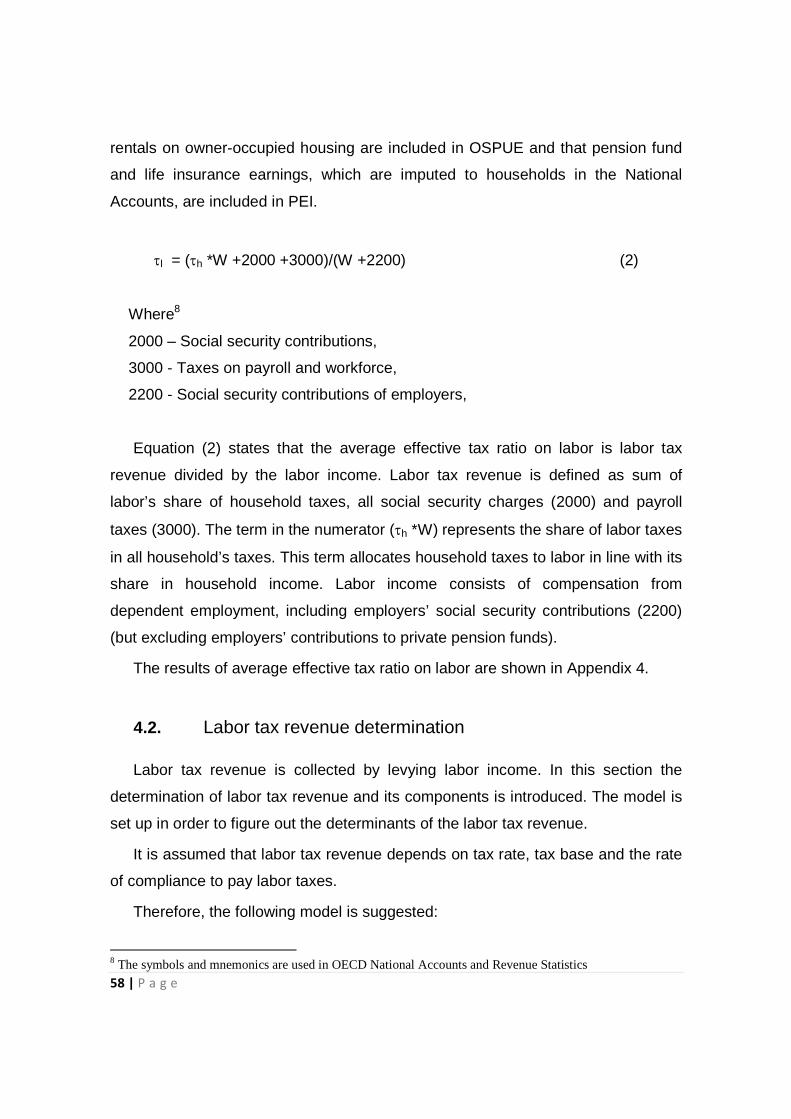
58 | P a g e
rentals on owner-occupied housing are included in OSPUE and that pension fund
and life insurance earnings, which are imputed to households in the National
Accounts, are included in PEI.
τl = (τh *W +2000 +3000)/(W +2200) (2)
Where8
2000 – Social security contributions,
3000 - Taxes on payroll and workforce,
2200 - Social security contributions of employers,
Equation (2) states that the average effective tax ratio on labor is labor tax
revenue divided by the labor income. Labor tax revenue is defined as sum of
labor’s share of household taxes, all social security charges (2000) and payroll
taxes (3000). The term in the numerator (τh *W) represents the share of labor taxes
in all household’s taxes. This term allocates household taxes to labor in line with its
share in household income. Labor income consists of compensation from
dependent employment, including employers’ social security contributions (2200)
(but excluding employers’ contributions to private pension funds).
The results of average effective tax ratio on labor are shown in Appendix 4.
4.2. Labor tax revenue determination
Labor tax revenue is collected by levying labor income. In this section the
determination of labor tax revenue and its components is introduced. The model is
set up in order to figure out the determinants of the labor tax revenue.
It is assumed that labor tax revenue depends on tax rate, tax base and the rate
of compliance to pay labor taxes.
Therefore, the following model is suggested:
8 The symbols and mnemonics are used in OECD National Accounts and Revenue Statistics

59 | P a g e
R�� = α�� × B�� × v�� (3)
Where
Rjt – revenue form labor tax for country j at time t,
αjt – the compliance rate for country j at time t,
Bjt – tax base – labor income for country j at time t,
vjt – labor tax rate for country j at time t.
In order to compare revenues among different countries the ratio to GDP is
included:
���� = α�� × β�� × v�� (4)
Where
Yjt – GDP at market prices for country j at time t,
βjt – tax base as a proportion of GDP for country j at time t.
The latter equation defines that labor tax revenue as a proportion of GDP will
increase directly with a tax rate, an increase in the tax base and increase in
compliance.
Tax rate, as depicted above, is derived as a ratio between labor tax revenue
and labor income using Mendoza et al. Therefore as for tax base the definite data
is used. Tax base (Bjt) is the product of average wage in country j at time t and total
labor force in country j at time t. This tax base could be referred as “potential” tax
base, showing the maximum possible size of the tax base if all the labor force
worked for average wage. That is the model is constructed with the assumption
that the maximum tax revenue can be collected if all the labor force worked for
current average wage and paid taxes of average effective tax ratio. However,
maximum revenue is not collected because current tax rate might be too high for

60 | P a g e
some individuals and they evade taxes by shifting to shadow or black economy.
The model assumes that unemployment is highly related to compliance to pay
taxes. Generally, tax base is reflected by formula:
B�� = w�� × L�� (5)
Where
wjt – average annual wage for country j at time t,
Ljt – total labor force for country j at time t.
Consequently,
β�� =���×���
��� (6)
The compliance ratio (αjt) is a function of “black economy” in a country.
Matthews (2003) uses currency to GDP ratio to measure the level of “black
economy”. He argues that argued that countries with a high ratio of currency to
GDP have a greater level of “black economy” activity and a lower compliance ratio
than countries with a lower currency to GDP ratio.
One of the determinants of the compliance ratio α is the level of black economy
is the level of black economy as a proportion of GDP as estimated by Schneider et
al, (2009). The empirical method used by Schneider et al is based on the statistical
theory of unobserved variables, which considers multiple causes and indicators of
the phenomenon to be measured, i.e. it explicitly considers multiple causes leading
to the existence and growth of the shadow economy, as well as the multiple effects
of the shadow economy over time. In particular, a Multiple Indicators Multiple
Causes (MIMIC) model – a particular type of a structural equations model (SEM) –
is used to analyze and estimate the shadow economies. The model uses variables
such as tax and social security contribution burdens, intensity of regulations, extent
of public sector services etc. With reference to Keen and Smith (1996) one can
assume that the incentive to evade is not linear in the tax rate and ambiguity is
captured by including quadratic term of the tax rate:
α�� = α(v��� ,m��) (7)

61 | P a g e
where mjt is the level of black economy as proportion to GDP in country j at time
t.
The full equation of labor tax revenue model is following:
���� = v�� × β�� × α(v��� , m��) (8)
4.3. The Data
The data for average effective tax ratio is collected from OECD Revenue
Statistics and Eurostat. The period of analysis covers 1965-2010 with some of
exceptions for several countries. The analysis is made for 11 EU countries and
Norway. Due to lack of the data we could not include more EU countries. For
example recent EU members provide data only since 1999, in some cases only
since 2004.
The main problem in the process of data collection was that only one country
(Germany) distinguishes tax revenue by different source of income – labor tax
revenue, capital tax revenue and corporate income tax revenue. Therefore, the
methodology of Mendoza, Razin, & Tesar (1994) was applied. Labor tax revenue is
considered to have the same weight in total income tax revenue as the wages and
salaries have in the sum of sum of the operating surplus of private unincorporated
enterprises, property and entrepreneurial income and wages.
Despite minor problems the empirical examples of most of the countries
illustrate humped shape of Laffer curve (Appendix 5). Figure 18 shows the scatter
plot of labor tax revenue as a percentage of GDP against average effective tax
ratio for all 463 observations.
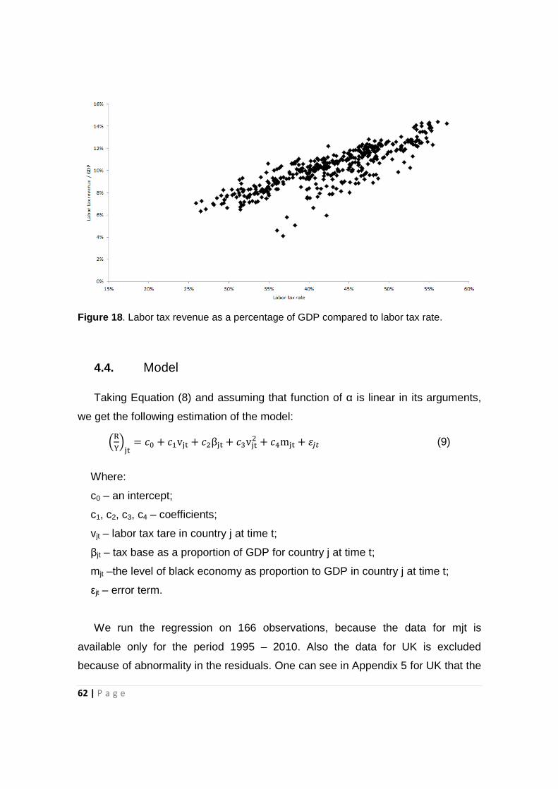
62 | P a g e
Figure 18. Labor tax revenue as a percentage of GDP compared to labor tax rate.
4.4. Model
Taking Equation (8) and assuming that function of α is linear in its arguments,
we get the following estimation of the model:
���� = �� + ��v�� + ��� + ��v��� + ��m�� + � ! (9)
Where:
c0 – an intercept;
c1, c2, c3, c4 – coefficients;
vjt – labor tax tare in country j at time t;
βjt – tax base as a proportion of GDP for country j at time t;
mjt –the level of black economy as proportion to GDP in country j at time t;
εjt – error term.
We run the regression on 166 observations, because the data for mjt is
available only for the period 1995 – 2010. Also the data for UK is excluded
because of abnormality in the residuals. One can see in Appendix 5 for UK that the

63 | P a g e
relation between labor tax rate and labor tax revenue as GDP is not humped
shaped but more random.
The primary results of the regression are shown in Table 24. Initial estimation
indicates that more than 87% of the dependent variable is explained by the model.
Also F-statistics show that the hypothesis that all the coefficients are null, can be
rejected. Contrary, all the coefficients are significant at the 2% level. As shown in
Figure 19 residuals are distributed normally – Jarque-Bera test does not reject
hypothesis of normal distribution of residuals.
Table 24. The output of the initial regression.
However, Durbin-Watson test indicates possibility of serial correlation – Durbin-
Watson statistics is 0.585, which is close to zero. Durbin-Watson statistic
measures the linear association between adjacent residuals from a regression
model. If the statistic is below about 1.5, it is a strong indication of positive first
order serial correlation (Vebbek, 2000).

64 | P a g e
Figure 19. The distribution of the residuals of the model.
Appendix 6 shows the correlogram for the first 36 lags. The correlogram has
spikes at lags up to four and at last five lags as well. The Q-statistics are significant
at all lags, indicating significant serial correlation in the residuals.
Additionally we perform Breusch-Godfrey Serial Correlation Lagrange multiplier
(LM) Test. This test belongs to the class of asymptotic tests. (Vebbek, 2000).
Unlike the Durbin-Watson statistic, the LM test may be used to test for higher order
autocorrelation errors and is applicable whether or not there are lagged dependent
variables. The results of LM test are shown in Table 25. Using the lag of 2 yields,
the test rejects the hypothesis of no serial correlation up to order two. Serial
correlation means that the residuals are correlated with their own lagged values.
This correlation violates the standard assumption of regression theory that
disturbances are not correlated with other disturbances.
Table 25. The output of Breusch-Godfrey Serial Correlation LM Test.
0
2
4
6
8
10
12
14
16
-0.015 -0.010 -0.005 0.000 0.005 0.010 0.015
Series: ResidualsSample 1 173Observations 166
Mean 2.46e-18Median -0.000220Maximum 0.017747Minimum -0.016697Std. Dev. 0.006416Skewness -0.106868Kurtosis 3.162675
Jarque-Bera 0.499013Probability 0.779185
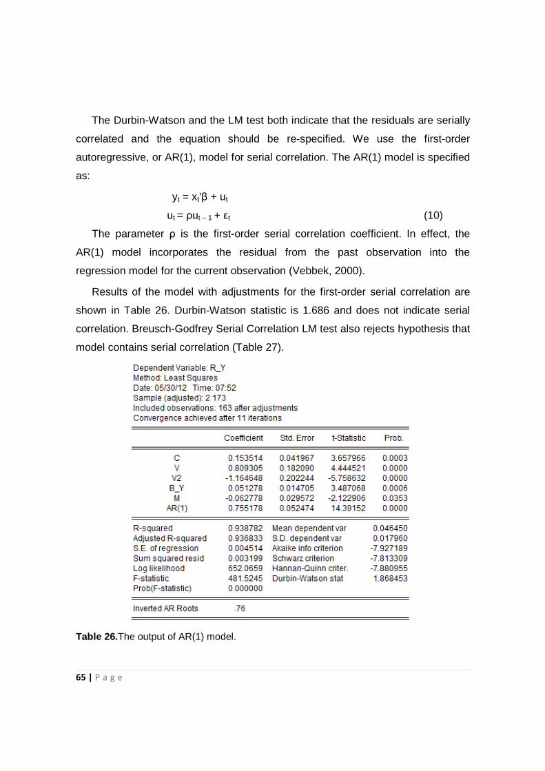
65 | P a g e
The Durbin-Watson and the LM test both indicate that the residuals are serially
correlated and the equation should be re-specified. We use the first-order
autoregressive, or AR(1), model for serial correlation. The AR(1) model is specified
as:
yt = xt’β + ut
ut = ρut – 1 + εt (10)
The parameter ρ is the first-order serial correlation coefficient. In effect, the
AR(1) model incorporates the residual from the past observation into the
regression model for the current observation (Vebbek, 2000).
Results of the model with adjustments for the first-order serial correlation are
shown in Table 26. Durbin-Watson statistic is 1.686 and does not indicate serial
correlation. Breusch-Godfrey Serial Correlation LM test also rejects hypothesis that
model contains serial correlation (Table 27).
Table 26.The output of AR(1) model.

66 | P a g e
Table 27. The output of Breusch-Godfrey Serial Correlation LM Test for AR(1) model.
It is has to be noted that all the coefficients are significant at 5 % level. T-
statistics show that for each coefficient separately and F-statistics reject hypothesis
that all the coefficients are equal to zero. Also R-squared is 0.9388, which shows
that the regression accounts for 93.88% percent of the variance in the dependent
variable. Figure 20 depicts fitted, actual residual values. The actual and fitted
values almost match each other, indicates high success of the regression in
predicting the values of the dependent variable within the sample.
Figure 20. Actual, fitted and residual values for AR(1) model.
Additionally, we use another method for dealing with serial correlation. The
method is called first difference method. It is a transformation on a time series
-.02
-.01
.00
.01
.02
.03
.00
.02
.04
.06
.08
.10
25 50 75 100 125 150
Residual Actual Fitted
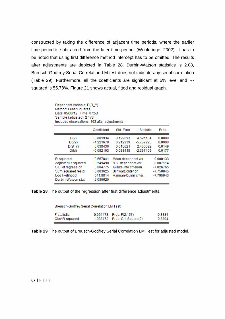
67 | P a g e
constructed by taking the difference of adjacent time periods, where the earlier
time period is subtracted from the later time period. (Wooldridge, 2002). It has to
be noted that using first difference method intercept has to be omitted. The results
after adjustments are depicted in Table 28. Durbin-Watson statistics is 2.08,
Breusch-Godfrey Serial Correlation LM test does not indicate any serial correlation
(Table 29). Furthermore, all the coefficients are significant at 5% level and R-
squared is 55.78%. Figure 21 shows actual, fitted and residual graph.
Table 28. The output of the regression after first difference adjustments.
Table 29. The output of Breusch-Godfrey Serial Correlation LM Test for adjusted model.

68 | P a g e
Figure 21. Actual, fitted and residual values for adjusted model.
Additionally we test if the variance of the error term is constant. If the error
terms do not have constant variance, they are said to be heteroskedastic. We use
White test to test for heteroskedasticity. Table 30 shows output of White test. With
F-statistics of 1.295 (p-value 0.22) we can reject hypothesis that error terms are
not constant.
Table 30. The output of White Heteroskedasticity Test.
-.04
-.02
.00
.02
.04
-.04
-.02
.00
.02
.04
.06
.08
25 50 75 100 125 150
Residual Actual Fitted
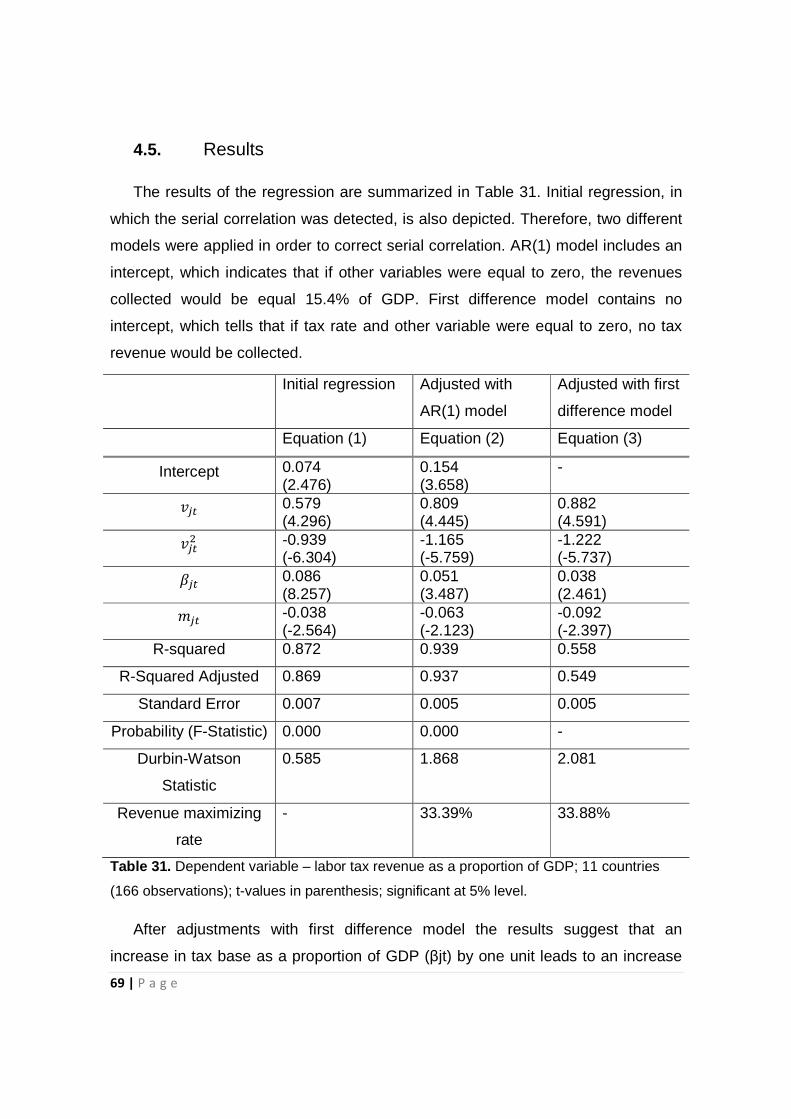
69 | P a g e
4.5. Results
The results of the regression are summarized in Table 31. Initial regression, in
which the serial correlation was detected, is also depicted. Therefore, two different
models were applied in order to correct serial correlation. AR(1) model includes an
intercept, which indicates that if other variables were equal to zero, the revenues
collected would be equal 15.4% of GDP. First difference model contains no
intercept, which tells that if tax rate and other variable were equal to zero, no tax
revenue would be collected.
Initial regression Adjusted with
AR(1) model
Adjusted with first
difference model
Equation (1) Equation (2) Equation (3)
Intercept 0.074 (2.476)
0.154 (3.658)
-
" ! 0.579 (4.296)
0.809 (4.445)
0.882 (4.591)
" !� -0.939 (-6.304)
-1.165 (-5.759)
-1.222 (-5.737)
# ! 0.086 (8.257)
0.051 (3.487)
0.038 (2.461)
$ ! -0.038 (-2.564)
-0.063 (-2.123)
-0.092 (-2.397)
R-squared 0.872 0.939 0.558
R-Squared Adjusted 0.869 0.937 0.549
Standard Error 0.007 0.005 0.005
Probability (F-Statistic) 0.000 0.000 -
Durbin-Watson
Statistic
0.585 1.868 2.081
Revenue maximizing
rate
- 33.39% 33.88%
Table 31. Dependent variable – labor tax revenue as a proportion of GDP; 11 countries
(166 observations); t-values in parenthesis; significant at 5% level.
After adjustments with first difference model the results suggest that an
increase in tax base as a proportion of GDP (βjt) by one unit leads to an increase

70 | P a g e
in labor tax revenue as a proportion of GDP by 0.038 units. Also there is an
indication that changes in “black economy” levels influence revenues collected. As
the results show, the change in black economy level as a proportion of GDP (mjt)
affects the change in labor tax revenue as a proportion of GDP by 0.092 units. This
conclusion could be a good suggestion to politicians to fight “black economy” more
actively because it can add more revenues to the budget.
Important point of the results is that quadratic term in tax rate is significant and
correctly signed. Thus, we calculate revenue maximizing labor tax rate. This is
done by finding derivate of each equation and setting the derivate to zero. We
found that revenues maximizing tax rate is 33.39% in AR(1) model and 33.88% in
first difference model. Many countries, such as Germany and Sweden, have higher
average tax rate than the maximizing one, therefore there is a room for labor tax
cuts, which would lead to even higher tax revenues. However for such countries as
Finland and UK, where average tax rate is lower than maximizing one, upward
changes in tax rate could raise political and social tension.
It has to be noted that the conclusions may not be accurate enough as there
are very few observations – only 166. The problem arises because of the lack of
data. For example, the methods and calculation for “black economy” levels are
available since 1995. Hopefully, bearing in mind that more qualitative and more
precise statistics are collected in these days, after a decade similar model will be
conducted and provide improved results.

71 | P a g e
5. VAT REVENUE ESTIMATION
As described in European Union law, the common system of VAT applies to the
production and distribution of goods and services bought and sold for consumption
within the European Union and the actual tax burden is visible at each stage in the
production and distribution chain. Generally, a value added tax resolves one of the
biggest drawbacks of a sales tax- omits the distortive effect of taxation on
intermediate consumption. To ensure that the tax is neutral in impact, irrespective
of the number of transactions, taxable persons for VAT may deduct from their VAT
account the amount of tax which they have paid to other taxable persons. VAT is
finally borne by the final consumer in the form of a percentage addition to the final
price of the goods or services. Double taxation is avoided and tax is paid only on
the value added at each stage of production and distribution (The European e-
Justice Portal under the European Commission). The main argument against VAT
is argued to be greater administrative and compliance costs because it envelopes
market participants in all stages of production and services, not only the final stage.
Since there are fixed costs of compliance that fall on the producers, it is generally
argued that VAT rates should not be levied at rates below 10%. Additionally,
extensive use of zero-rating and tax exemptions can substantially increase the
costs of VAT (Hagemann et al, 1988)
Even though the potential for evasion is believed to be reduced by the self –
policing nature of the value added taxes, European authorities have recently and
with growing concern addressed the VAT gap problem. The ‘Study to quantify and
analyse the VAT gap in the EU-25 Member States’ report issued on 21st
September 2009 the impact of the VAT gap in the member states. VAT gap is
described as the gap between the amount of value added tax due and the amount
received by the member states. VAT gap is not a measure of VAT fraud instead for
example it might include VAT not paid as a result of legitimate tax avoidance
measures and VAT not collected due to insolvencies. The VAT gap is primarily
estimated on national accounts data and depends on the accuracy and
completeness of the data, thus it might not take into account some activities that

72 | P a g e
are outside the scope of national accounts. The VAT gap in the period of year 2000
to 2006 is estimated to be as high as 30 percent of the aggregate theoretical tax
base.
As presented in the above mentioned report, there is a lack of data for the
estimation of VAT fraud, since:
• (a)’published data on the size of different types of VAT fraud are insufficient to
piece together an estimate of VAT fraud in the economy as a whole.
• (b) There may be a selection bias. Presenting the value of the different types of
VAT fraud detected by tax agencies, as reported by some in annual reports,
would risk giving a distorted account of the relative importance of different
types of VAT fraud as well as of overall level of VAT fraud.
• (c) The raw data underlying the estimates of particular types of VAT are based,
almost invariably, on operational data held by the tax agencies. Generally,
these are confidential, as are the methods used to derive them.’
5.1. VAT Revenue Determination
This section will set out a framework for the determination of VAT revenues by
the decomposition of its components and the modeling of the determinants of the
VAT base. In the broader sense, VAT revenues will depend on the VAT base, the
VAT rate and the compliance rate. The following model is suggested:
R�� = α�� × B�� × v�� (11)
Where:
Rjt – VAT revenue for country j at time t;
αjt – the compliance rate as a proportion of GDP at market prices for country j at
time t;
Bjt – VAT base for country j at time t;
vjt – the representative VAT rate for country j at time t;

73 | P a g e
In order to compare revenues among different countries the ratio to GDP is
included:
���� = α�� × β�� × v�� (12)
Where:
Yjt – GDP at market prices for country j at time t,
βjt – tax base as a proportion of GDP at market prices for country j at time t.
Equation (12) is used for the comparability of the VAT revenue results between
all member states. It states that VAT revenue as a proportion of GDP will increase
directly with the VAT rate, an increase in the VAT base as a proportion of GDP,
and an increase in compliance.
The weighted average value added tax rate would be the appropriate measure
of the representative VAT rate. However such data is not readily available for most
countries and if available it would significantly limit our sample due to the irregular
intervals available. The standard VAT rate will be used as a proxy for the weighted
average value added tax rate.
Despite the fact that value added taxes are relatively uniform in their
application, the VAT base differs significantly from country to country. The VAT
base will be proxied by the VAT revenue ratio which is the proportion of actual VAT
revenue to final consumption adjusted by the tax revenue. VAT base is derived
from the final consumption expenditure accounts which are calculated based on
purchasers’ price. According to the European System of Accounts (ESA 95 3.06
and 3.92), purchasers’ price is the price the purchaser actually pays for the
products; including any taxes less subsidies on the products (but excluding
deductible taxes like VAT on the products), etc. The second proportion expresses
the VAT base a percentage of GDP. The arguments of the function are presented
as available in the Eurostat statistic databases:

74 | P a g e
B�� =%�����
&��×('���(%�����)× '���
*%'�� (13)
Where:
D211�� – value added type tax revenues;
P3�� – final consumption expenditure;
012 ! – gross domestic product;
An additional argument is added in order to evaluate the appearance of cross-
border trading between member states. We sought to evaluate the extent of cross
border trading originating from the fundamental differences in the application of
VAT amid member states. We employed a variable representing the VAT gap (G��) – an estimate that was presented by Reckon LLP, (2009) in a European
Commission report (see Study to quantify and analyse the VAT gap in the EU-25
Member States). VAT generally indicates the effect of reduced and zero rating of
the tax base and can be argued to be one of the factors determining the distinct
volumes of cross-border trading in the EU member states. The VAT base is
expressed by:
β�� = β(B��, G��) (14)
The compliance rate ‘α’ is the function of the shadow economy in a country. It
may be argued that the extent of tax evasion and tax fraud is dependent on the
national cultural and economic factors, on the perception of the quality of life and
other qualitative factors causing distortions in the compliance rate. We are lacking
substantial data both for quantitative and qualitative factors for the compliance rate
therefore a model estimating the aggregate compliance rate will be employed.
75 | P a g e
As for the base of our compliance rate we will use data of the shadow economy
as estimated by Schneider et al, (2009). The extent of the shadow economy is
expressed as a proportion of GDP in market prices for each of the European Union
member countries. Previous studies of Schneider (1994b, 2000, 2004, 2005 and
2007) and Johnson, Kaufmann and Zoido-Lobatón (1998a, 1998b) found
statistically significant evidence for the influence of taxation on the shadow
economy suggesting a connection between the compliance rate and the extent of
the shadow economy. The estimates in question are aimed at quantifying the
aggregate extent of the shadow economy therefore we will try to model the
compliance rate for VAT.
As proposed by Kent Matthews (2003), the theory of direct tax evasion is
ambiguous on the effect of tax rates on evasion. A higher tax rate will increase the
incentive to evade, but evasion is a risky activity and greater risk could result in
increased compliance. The standard results regarding the ambiguity of the effect of
the tax rate on the compliance ratio follows through the assumption of risk
aversion. However, Cremer & Gahvari (1993) show that compliance decreases for
an increase in the indirect tax rate in the case of a competitive risk neutral firm. The
incremental change of the tax rate can be also argued as an important factor and
will be added to the model.
The number of VAT rates is another factor leading to possible tax avoidance.
Agha & Haughton, (1996) suggest, that the compliance rate depends on the level
of the average value added tax rate and on the presence of multiple tax rates.
Thus the higher the number of VAT rates, the higher possibility to misclassify
goods and the lower the compliance ratio. The ambiguity of the effect of the value
added tax rate on compliance is captured by a quadratic term in the VAT rate since
it is reasonable to assume that the incentive to evade is non-linear in the tax rate,
Kent Matthews, (2003).
Statistical economic data suggests the existence of significant underlying
differences between EU member states based on the date of their accession to the
Union with the newest member states showing a significantly higher level of
shadow economy and non – compliance. In order to reflect the transitional state of
76 | P a g e
the countries that have experienced a shift from a planned economy to a free
economy and to compensate for the distortions a dummy variable will be added to
the equation with the value of =1 will be attributed to the ex – members of the
Warsaw Pact zone, and =0 for the EU – 15 member states and Malta, Cyprus and
Slovenia. Based on the presumptions presented above, the compliance rate will be
estimated as:
α�� = α(v��, v��� , m��, N��, ∆v��, Dum��) (15)
Combining equations (14) and (15) into the equation (12), we can finalize the
model as:
���� = (v��, v��� , m��, N��, ∆v��, Dum��, B��, G��) (16)
5.2. The Data
We have collected a balanced panel of data on 25 countries of the EU, omitting
Romania and Bulgaria from the sample due to a shortage of data inputs. The
estimation period has been drastically curtailed because of data availability issues
connected to the VAT base and compliance. The bulk of statistical information
used in the estimation was obtained from Eurostat databases. Information on the
historical tax rates and their reductions was drawn from a European Commission
taxation paper VAT Rates Applied in the Member States of the European Union,
Situation at 1st January 2012.
Ideally, the weighted average VAT rate would be most appropriate measure of
the effective VAT rate. However, the weighted rates are considered confidential
data by the Directorate-General for Budget, European Commission and could only
be acquired for a single year. The use of the standard rate is based on two factors:
most of VAT-rated consumer spending is taxed at the standard rate across the EU,
and the correlation between the available weighted average tax rates and standard
rates for the sample was 0,923. Even though it does not provide information about
77 | P a g e
the correlation of the rates over the full sample it serves as an indicator of the
cross-section variation of the rates.
Schneider et al, (2010) base their estimation of the shadow economy on the
following definition: ‘the shadow economy includes all market-based legal
production of goods and services that are deliberately concealed from public
authorities for any of the following reasons:
• to avoid payment of income, value added or other taxes;
• to avoid payment of social security contributions;
• to avoid having to meet certain legal labor market standards, such as minimum
wages, maximum working hours, safety standards, etc.;
• to avoid complying with certain administrative procedures, such as completing
statistical questionnaires or other administrative forms.’
The empirical method used by Schneider et al, (2010) is based on the statistical
theory of unobserved variables, which considers multiple causes and indicators of
the phenomenon to be measured, i.e. it explicitly considers multiple causes leading
to the existence and growth of the shadow economy, as well as the multiple effects
of the shadow economy over time. In particular, a Multiple Indicators Multiple
Causes (MIMIC) model – a particular type of a structural equations model (SEM) –
is used to analyze and estimate the shadow economies. Previous studies of
Schneider found statistically significant evidence for the influence of taxation on the
shadow economy.
Our dataset was severely trimmed by the availability of data and constituted of
135 observations for 23 member states (excl. Romania, Bulgaria, Denmark and
Cyprus). The humped shape of the variables is evident in Figure 22.

78 | P a g e
Figure 22. . VAT revenue as a percentage of GDP compared to VAT rate
5.3. Model
Taking Equation (16) and assuming that function of α is linear in its arguments,
we get the following estimation of the model:
���� = �� + ��v�� + ��v��� + ��m�� + ��N�� + �7∆v�� + �8Dum�� + �9B�� + �:G�� + � ! (17)
Where:
�� – the intercept;
��, ��, ��, ��, �7, �8, �9 – coefficients;
� ! – error term for country j at time t;
Hsing, (1996) argues, that in empirical work additional functional forms like the
log-log and the semi-log (the log-linear and the linear-log) should be used to
identify a form that better fits the sample and Laffer curve.
4%
5%
6%
7%
8%
9%
10%
12% 14% 16% 18% 20% 22% 24%
VA
T r
ev
en
ue
to
GD
P
VAT rate
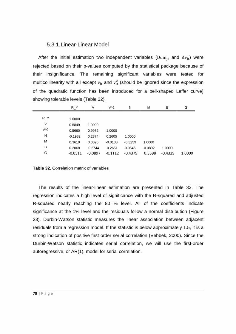
79 | P a g e
5.3.1. Linear-Linear Model
After the initial estimation two independent variables (Dum�� and ∆v��) were
rejected based on their p-values computed by the statistical package because of
their insignificance. The remaining significant variables were tested for
multicollinearity with all except v�� and v��� (should be ignored since the expression
of the quadratic function has been introduced for a bell-shaped Laffer curve)
showing tolerable levels (Table 32).
R_Y V V^2 N M B G
R_Y
1.0000 V
0.5849 1.0000 V^2
0.5660 0.9982 1.0000 N
-0.1982 0.2374 0.2605 1.0000 M
0.3619 0.0026 -0.0133 -0.3259 1.0000 B
0.2068 -0.2744 -0.2651 0.0546 -0.0892 1.0000 G
-0.0511 -0.0897 -0.1112 -0.4379 0.5598 -0.4329 1.0000
Table 32. Correlation matrix of variables
The results of the linear-linear estimation are presented in Table 33. The
regression indicates a high level of significance with the R-squared and adjusted
R-squared nearly reaching the 80 % level. All of the coefficients indicate
significance at the 1% level and the residuals follow a normal distribution (Figure
23). Durbin-Watson statistic measures the linear association between adjacent
residuals from a regression model. If the statistic is below approximately 1.5, it is a
strong indication of positive first order serial correlation (Vebbek, 2000). Since the
Durbin-Watson statistic indicates serial correlation, we will use the first-order
autoregressive, or AR(1), model for serial correlation.
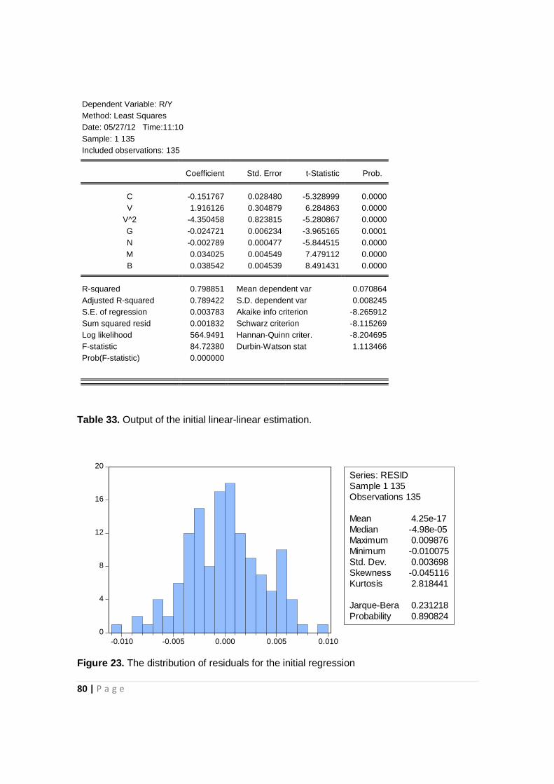
80 | P a g e
Dependent Variable: R/Y Method: Least Squares Date: 05/27/12 Time:11:10 Sample: 1 135 Included observations: 135
Coefficient Std. Error t-Statistic Prob.
C -0.151767 0.028480 -5.328999 0.0000 V 1.916126 0.304879 6.284863 0.0000
V^2 -4.350458 0.823815 -5.280867 0.0000 G -0.024721 0.006234 -3.965165 0.0001 N -0.002789 0.000477 -5.844515 0.0000 M 0.034025 0.004549 7.479112 0.0000 B 0.038542 0.004539 8.491431 0.0000
R-squared 0.798851 Mean dependent var 0.070864 Adjusted R-squared 0.789422 S.D. dependent var 0.008245 S.E. of regression 0.003783 Akaike info criterion -8.265912 Sum squared resid 0.001832 Schwarz criterion -8.115269 Log likelihood 564.9491 Hannan-Quinn criter. -8.204695 F-statistic 84.72380 Durbin-Watson stat 1.113466 Prob(F-statistic) 0.000000
Table 33. Output of the initial linear-linear estimation.
Figure 23. The distribution of residuals for the initial regression
0
4
8
12
16
20
-0.010 -0.005 0.000 0.005 0.010
Series: RESIDSample 1 135Observations 135
Mean 4.25e-17Median -4.98e-05Maximum 0.009876Minimum -0.010075Std. Dev. 0.003698Skewness -0.045116Kurtosis 2.818441
Jarque-Bera 0.231218Probability 0.890824

81 | P a g e
After the adjustment, the Durbin-Watson statistic exceeds the value of 1.5
indicating that the hypothesis of no serial correlation can be accepted. It has to be
noted, that after the adjustment the coefficients are significant at the 1 % level and
the R-squared and adjusted R-squared projects a high level of significance
exceeding 85 %. The value of coefficient c� has a negative value thus confirming a
bell-shaped Laffer curve for the sample for the linear-linear estimation (Table 33).
We also test for the indications of heteroskedasticity – to check if the variance of
the error term is constant. If the error terms do not have constant variance, they
are said to be heteroskedastic. We use the White test which produces the value of
F-statistic equal to 1.47 (p-value 0.0885), signifying that we can accept the null
hypothesis of constant error terms. We do not identify strong outliers for the
residual sample of the AR(1) adjusted model (Figure 24).
According to optimization theory, tax revenue is maximized when the first order
derivative of VAT revenue to GDP with respect to the VAT rate is set equal to zero,
assuming that the coefficient of the quadratic term assumes a negative value
otherwise the tax revenue minimizing rate would be calculated and the Laffer
principle violated.

82 | P a g e
Dependent Variable: R/Y Method: Least Squares Date: 05/27/12 Time:101:11 Sample (adjusted): 2 135 Included observations: 134 after adjustments Convergence achieved after 12 iterations
Coefficient Std. Error t-Statistic Prob.
C -0.199409 0.055125 -3.617404 0.0004 V 2.571848 0.599064 4.293106 0.0000
V^2 -6.329918 1.621351 -3.904101 0.0002 G -0.019332 0.005522 -3.500977 0.0006 N -0.001379 0.000436 -3.162574 0.0020 M 0.030692 0.005359 5.727234 0.0000 B 0.022272 0.004498 4.951637 0.0000
AR(1) 0.664340 0.068474 9.702030 0.0000
R-squared 0.859624 Mean dependent var 0.070755 Adjusted R-squared 0.851825 S.D. dependent var 0.008177 S.E. of regression 0.003148 Akaike info criterion -8.626461 Sum squared resid 0.001248 Schwarz criterion -8.453455 Log likelihood 585.9729 Hannan-Quinn criter. -8.556157 F-statistic 110.2271 Durbin-Watson stat 2.117891 Prob(F-statistic) 0.000000
Inverted AR Roots .66
Table 33. Output of AR(1) adjusted regression
Heteroskedasticity Test: White
F-statistic 1.469760 Prob. F(26,107) 0.0885 Obs*R-squared 35.26280 Prob. Chi-Square(26) 0.1061 Scaled explained SS 67.84692 Prob. Chi-Square(26) 0.0000
Table 34. Output of White Heteroskedasticity test

83 | P a g e
Figure 24. Actual, fitted and residual values for the AR(1) adjusted estimation
5.3.2. Log- Log Model
We will estimate alternative functional forms, namely the log-log form, as
specified by Hsing, (1996). In the log-log form, the coefficients are the elasticities,
which are assumed to be the same during the sample period. Taking logs of
equation (16) we arrive at:
ln ���� = �� + ��ln(v��) + ��>?(v��)� + ��ln(m��) + ��ln(N��) + �7 ln@∆v��A +
�8ln(Dum��) + �9ln(B��) + �:ln(G��) + � ! (18)
The equation is regressed on the same set of observations for the full list of
independent variables and the model is adjusted for the insignificant variables just
as the linear-linear form. Ln(Dum��) and ln(∆v��) are rejected due to non positive
number value issues. Ln(G��)is rejected based on insignificance (probability of
0.337). The subsequent model displays robust qualities with all of the variables
significant at the 1 % level and the R-squared and adjusted R-squared exhibiting
-.008
-.004
.000
.004
.008
.012
.05
.06
.07
.08
.09
25 50 75 100 125
Residual Actual Fitted

84 | P a g e
sufficient significance of 78 % – 79 % (see appendix 7). The residuals display
properties of normal distribution (Jarque-Bera of 1.819549 with the probability of
0.403, see Figure 25) therefore we continue with tests for auto-correlation and
heteroskedasticity.
Figure 25. The distribution of residuals of the initial log-log model
The Durbin-Watson statistic displays a value of 1.006 which suggests that
autocorrelation exists therefore we apply the AR(1) model just like in the linear-
linear form. The intermediate estimation output is presented in Appendix 8. ln(N��)
is rejected due to insignificance (probability of 0.1889). The Durbin-Watson statistic
for AR(1) adjusted model is 2.033 and does not indicate serial correlation. Once
again we use the White test which produces the value of F-statistic equal to 1.78
(p-value 0.0584), signifying that we can accept the null hypothesis of constant error
terms (Table 35). We do not identify strong outliers for the residual sample of the
AR(1) adjusted model (Figure 26).
0
2
4
6
8
10
12
14
-0.15 -0.10 -0.05 0.00 0.05 0.10
Series: RESIDSample 1 135Observations 135
Mean 1.63e-15Median 0.005697Maximum 0.131565Minimum -0.154806Std. Dev. 0.053739Skewness -0.275387Kurtosis 2.858143
Jarque-Bera 1.819549Probability 0.402615

85 | P a g e
Heteroskedasticity Test: White
F-statistic 1.782242 Prob. F(12,121) 0.0584 Obs*R-squared 20.12717 Prob. Chi-Square(12) 0.0647 Scaled explained SS 38.51611 Prob. Chi-Square(12) 0.0001
Table 35. Output of White Heteroskedasticity test for log-log
The final AR(1) adjusted log-log estimation is significant at the 1 % level and
produces R-squared and adjusted R-squared values exceeding 85 %, implying a
high level of significance. Statistical tests indicate that the error terms are not auto-
correlated and are homoskedastic. The coefficient values support the humped
shape of the Laffer curve and allow us to calculate the VAT revenue maximizing
tax rate (Table 36). Additionally we attempted to employ the first difference model,
but the subsequent coefficient did not support the bell shaped curve and the overall
significance of the model was under 10%, suggesting that no valid conclusions
could be drawn from the model.
Figure 26. Actual, fitted and residual values for the AR(1) adjusted log-log estimation
-.15
-.10
-.05
.00
.05
.10
.15
.20
-3.0
-2.9
-2.8
-2.7
-2.6
-2.5
-2.4
25 50 75 100 125
Residual Actual Fitted

86 | P a g e
Dependent Variable: LOG(R/Y) Method: Least Squares Date: 05/27/12 Time: 11:15 Sample (adjusted): 2 135 Included observations: 134 after adjustments Convergence achieved after 10 iterations
Coefficient Std. Error t-Statistic Prob.
C -9.708906 2.282341 -4.253924 0.0000 LOG(V) -9.260168 2.672665 -3.464770 0.0007
LOG(V)^2 -2.900493 0.782417 -3.707094 0.0003 LOG(M) 0.078993 0.013872 5.694525 0.0000 LOG(B) 0.265414 0.036618 7.248280 0.0000 AR(1) 0.686951 0.066574 10.31856 0.0000
R-squared 0.859430 Mean dependent var -2.655220 Adjusted R-squared 0.853939 S.D. dependent var 0.116510 S.E. of regression 0.044528 Akaike info criterion -3.341677 Sum squared resid 0.253785 Schwarz criterion -3.211923 Log likelihood 229.8923 Hannan-Quinn criter. -3.288949 F-statistic 156.5161 Durbin-Watson stat 2.033227 Prob(F-statistic) 0.000000
Inverted AR Roots .69
Table 36. Final AR(1) adjusted log-log estimation output
The initial and subsequent estimations of a semi-log model would not produce a
negative coefficient for the quadratic term meaning that any interpretations of the
model would be void and a U-shaped Laffer Curve would be plotted thus
contradicting the Laffer theory.
5.4. Results
The results of the regressions are summarized in Table 37. Initial Linear-Linear
regression, in which the serial correlation was detected, is also depicted, but the
maximizing rate is not calculated. The models include an intercept since data
points are available only in a limited range of tax rate values and it would not be

87 | P a g e
possible to extrapolate the tax rate from 0 % to 100%. The same applies to the
initial Log-Log.
Initial Linear-Linear
regression
AR(1) adjusted
Linear-Linear regression
Initial Log-Log
regression
AR(1) adjusted Log-Log
regression
Intercept -0.151767
(-5.328999) -0.199409 (-3.617404)
-6.403651 (-5.494488)
-9.708906 (-4.253924)
" ! 1.916126
(6.284863) 2.571848 (4.293106)
-5.738982 (-4.208469)
-9.260168 (-3.464770)
" !� -4.350458 (-5.280867)
-6.329918 (-3.904101)
-1.928708 (-4.820699)
-2.900493 (-3.707094)
0 ! -0.024721 (-3.965165)
-0.019332 (-3.500977) - -
B !
-0.002789 (-5.844515)
-0.001379 (-3.162574)
-0.055023 (12.03949) -
$ !
0.034025 (7.479112)
0.030692 (5.727234)
0.081697 (6.645544)
0.078993 (5.694525)
C !
0.038542 (8.491431)
0.022272 (4.951637)
0.401906 (-3.334546)
0.265414 (7.248280)
AR(1) - 0.66434 (9.702030) -
0.686951 (10.31856)
R-squared 0.798851 0.859624 0.790085 0.85943 R-Squared Adjusted 0.789422 0.851825 0.781949 0.853939
Standard Error 0.003783 0.003148 0.054771 0.044528 Probability (F-Statistic) 0.000000 0.000000 0.000000 0.000000 Durbin-Watson Statistic 1.113466 2.117891 1.00613 2.033227
Revenue maximizing rate - 20.57% - 20.26%
Table 37. Dependent variable – VAT revenue as a proportion of GDP; 23 countries (135 observations); t-values in parenthesis.
In the linear form the slope remains constant while in the Log-Log form the
coefficient is the elasticity, which is assumed to be the same during the sample
period. Coefficient values of the quadratic term support thr bell shaped Laffer curve
and allow us to calculate the revenue maximizing rates, which are relatively
uniform, with the maximizing rate between 20.26 % and 20.57 %. Matthews, K.
(2003) present a slightly lower range for the maximising rate at 18.0 % - 19.3 %.
The differences can be justified by the widening of the sample – all of the member
states of the 2004 enlargement stage are included. A sharp increase in the
average VAT rate for EU was visible in the period of 2008 and 2010 with the

88 | P a g e
average rate reaching 20.19%. The uniform actions of raising VAT rates across the
Union suggest that the rates were on the upward slope of the curve, but caution
should be practiced when debating additional VAT rate hikes, because according
to our research the rates are close to the theoretical maximising rates and might
easily sway to the prohibitive side of the curve.
Coefficients of the VAT gap estimate support our assumption that the increasing
extent of zero and reduced VAT rating stimulate surplus cross-border trading. The
assumption of negative effect of the number of officially administered on the VAT
revenue was also affirmed, as indicated by the negative coefficient values.
According to the coefficients, an increase in the VAT base corresponds in an
increase of VAT revenue.
Controversial conclusions can be drawn from the shadow economy estimates,
since according to the coefficient values an increase in the shadow economy and
simultaneously in VAT fraud would result in growing VAT revenue. The
discrepancy might be caused by error of the estimation of shadow economy,
because it is not hard data and should be interpreted with caution.
Finally, it has to be noted that the conclusions may not be accurate enough as
there are very few observations – only 135. The lack of data constitutes the
greatest obstacle in quantifying the tax revenue curve and we can only hope that
more frequent and obtainable data will be accessible in the future for the estimation
of optimizing tax rates.
89 | P a g e
6. CONCLUSION
Labor taxes and value added taxes are the most substantial taxes levied on
individuals. Therefore upward or downward changes of these taxes are of sensitive
nature to the wider society. On the other hand the level of these taxes is important
for the state’s budget, as in most European countries labor tax revenue accounts
for about half of all taxes collected, while VAT revenue accounts for more than a
fifth of total tax revenues. The goal of each government is to set such tax rates
which would be acceptable for the society at the same time maximizing the tax
revenue. The theory of the Laffer Curve explains the relationship between tax
revenue and tax rate. The question is whether the theory works in practice.
The results of the analysis performed in this paper support the notion of the
Laffer Curve representing a bell shaped arch. Both the function of VAT revenue
and the function of labor tax revenue are parabolic and illustrate that efficiency of
the tax system declines with an increase in tax rates. Labor tax revenue is
positively dependent on tax base and tax rate itself. However the level of the black
economy negatively influences labor tax revenue. The same dependency applies
to VAT revenue just additionally we found that the number of tax rates is significant
and has an impact on VAT revenue. The only controversial observation was the
positive effect of an increase in the shadow economy on VAT revenue collection.
This distortion could be justified by the soft nature of the shadow economy
estimates and should be interpreted with an appropriate level of tolerance
In order to test how Laffer Curve works out with real-life data, the quadratic term
of the tax rates was introduced. It was found to be significant with the correct sign
of the coefficient. The quadratic term allows for the computation of revenue
optimizing tax rates. As for the labor tax rate, we found that the revenue
maximizing tax rate is in the range of 33.39 – 33.88 per cent. VAT revenue
maximizing tax rate lies in the range of 20.26 % – 20.57 % Countries such as
France, Austria and Belgium have higher average labor tax rates than the
maximizing one, therefore tax cuts should be considered. Accordingly this would

90 | P a g e
lead to even higher tax revenues. However, for countries such as Greece, Finland
and UK, where average tax rates are lower, upward changes in tax rates could
raise political and social tension. As for VAT rates, countries like Denmark,
Sweden, Hungary and Finland seem to be positioned on the prohibitive slope of
the curve and should introduce tax cuts while Spain, Malta, Luxembourg and
Germany could benefit from an increase in tax rates. Additionally, and expansion of
the VAT base that is taxed on the standard rate could be an efficient measure of
generating additional tax revenue.

91 | P a g e
7. REFERENCES
1. Agell, J., Mats, P., 2000, „On the Analystics of the Dynamic Laffer Curve”, Working
paper, pp. 1-26.
2. Agha, A., Haughton, J., 1996, “Designing VAT systems: some efficiency
considerations”, Review of Economics and Statistics, LXXVIII, 2, pp. 303–308.
3. Auerbach, A.J., 1985. The theory of excess burden and optimal taxation. In: Auerbach, A.J., Feldstein, M. (Eds.), Handbook of Public Economics. North-Holland, Amsterdam.
4. Becsi Z., 2000, The shifty Laffer curve, Economic Review - Federal Reserve Bank
of Atlanta, Third Quarter.
5. Begg, D., 1998, „Pegging Out: Lessons from the Czech Exchange Rate Crisis“, Journal of comparative economics 26, 669–690.
6. Burda, M., Wyplosz, C., 1993, Macroeconomics: A European Text, OUP, New
York.
7. Cameron, F. , 2010, The European Union as a Model for Regional Integration,
Council on Foreign Relations working paper.
8. Cremer, H., Gahvari, F., 1993, “Tax evasion and optimal commodity taxation”,
Journal of Public Economics, 50, pp. 261–275.
9. Danish Tax reform 2010, 2009, Paper to the OECD WP 2 meeting, The Danish
Ministry of Taxation.
10. Eurostat Databases, https://ec.europa.eu/eurostat
11. Feige, E.L., McGee, R.T., 1983, „The Unobserved Economy and the UK. Laffer
Curve”, Journal of Economics, 85 (4), pp. 499-519.
12. Friedman, E., Johnson, S., Kaufmann, D., Zoido-Lobaton, P., 2000, “Dodging the
grabbing hand: the determinants of unofficial activity in 69 countries”, Journal
Public Economics 76 (3), pp. 459–493.
13. Haan P., Steiner V, 2005, Labor Market Effects of the German Tax Reform 2000,
Discussion Papers, German Institute of Economic Research.
14. Hagemann, R. P., Jones, B. R. & Montador, R. B., 1988 “Tax reform in OECD
countries: motives, constraints and practice”, OECD Economic Studies, 10, Spring,
pp. 85–226.

92 | P a g e
15. Heijman W.J.M., van Ophem, J.A.C., 2005, “Willingness to pay tax. The Laffer
curve revisited for 12 OECD countries”, The Journal of Socio-Economics 34, pp.
714–723.
16. Henderson D., 1981, “Limitations of the Laffer Curve as a justification for tax cuts”,
Cato Journal, vol. I, No. 1 Spring.
17. Hill, R. W., Holland, P. W., 1977 „Two robust alternatives to least squares
regression“, Journal of the American Statistical Association, Vol. 72, No. 360 (Dec.,
1977), pp. 828-833
18. Hsing, Y., 1996, „Estimating the Laffer curve and policy implications“, Journal of
Socio-Economics, 3(25), pp. 395–401.
19. Ireland, P. N., 1994, “Supply-side economics and endogenous growth”, Journal Of
Monetary Economics 33, pp. 559-572.
20. Jarass L., Obermair G.M., 1997, More Jobs, Less Tax Evasion, Cleaner
Environment, Report commissioned by the European Commission.
21. Jensen, C. B., Slapin, J. B., 2010, Institutional Hokey-Pokey: The Politics of
Multispeed Integration in the European Union, UCD Dublin European Institute
Working Paper 10-1, p. 10-11.
22. Kee, M., Smith S., 1996, “The future of Value Added Tax in the European Union”,
Economic Policy, 23, October, pp. 375–420.
23. Keen, M. & Smith, S., 1996, “The future of Value Added Tax in the European
Union”, Economic Policy, 23,October, pp. 375–420.
24. Kominkova, Z., 1999, Monetary and Exchange Rate Policy in Slovakia, National
Bank of Slovakia, Bratislava.
25. Laffer, A.B., 1986, “The Ellipse: an explanation of the Laffer curve in a two-factor
model”, In Canton, V.A., Kadlec, C.W., Laffer, A.B. (Eds.), The Financial Analyst’s
Guide to Fiscal Policy, Greenwood Press, New York, pp. 1–35.
26. Lindsey, L. B., 1987, “Individual taxpayer response to tax cuts: 1982-1984: With
implications for the revenue maximizing tax rate”, Journal of Public Economics
33(2), pp. 173-206.
27. Malcomson, J., 1986, “Some analytics of the Laffer curve”,. Journal of Public
Economics 29, 263–279.
28. Matthews K., “VAT Evasion and VAT Avoidance: Is there a European Laffer curve
for VAT?”, International Review of Applied Economics, 17: 1, pp. 105 — 114.

93 | P a g e
29. Meidūnas, V., Puzinauskas, P., 2001, Mokesčiai: Teorija, Vaidmuo, Raida, VĮ
Teisinės informacijos centras, Vilnius, pp 6-38.
30. Mendoza E. G., Razin A., Tesar L.L., 1994, “Effective tax rates in macroeconomics.
Cross-country estimates of tax rates on factor incomes and consumption,” Journal
of Monetary Economics, 34 (3), pp. 297–323.
31. Mendoza E.G., Milesi-Ferretti G.M., Asea P., 1997, “On the ineffectiveness of tax
policy in altering long-run growth: Harberger’s superneutrality conjecture,” Journal
of Public Economics, 66 (1), pp. 99–126.
32. Mitchell D.J., 2009, “The Laffer Curve: Understanding the Relationship Between
Tax Rates, Taxable Income, and Tax Revenue”, Prosperitas, Vol. IX, Issue I.
33. Novales, A., Ruiz, J., 2002, „Dynamic Laffer curves”, Journal of Economic
Dynamics & Control, 27, pp. 181-206.
34. OECD 1998, The Tax/Benefit Position of Employees 1995-1996. Paris. OECD.
35. OECD Databases, http://www.oecd-ilibrary.org/
36. Reckon LLP, 2009, Study to quantify and analyse the VAT gap in the EU-25
Member States, European Comission, 5-11.
37. Reiss L., Toglhofer W., 2011, “Austria’s Tax Structure in International Comparison
– A Statistical and EconomicAnalysis”, Monetary Policy&Economy, Q1/11.
38. Schneider, F., Buehn, A., Montenegro, C. E., 2010, Shadow Economies all over
the World: New Estimates for 162 Countries from 1999 to 2007, Policy research
working paper, The World Bank.
39. Schratzenstaller, M. 2007, “WIFO-Weißbuch: Wachstumsimpulse durch die
öffentliche Hand”, In: WIFO-Monatsberichte 80(6). 509–526.
40. Smith A., 1904 An Inquiry into the Nature and Causes of the Wealth of Nations,
London: Methuen and Co., Ltd., ed. Edwin Cannan.
41. Stačiokas, R.,Rimas J., 2003, Mokesčiai: Istorinė Raida ir Dabartis, Kaunas
‘Technologija’, Kaunas.
42. Stuart, C., 1981, “Swedish tax rates, labor supply and tax revenues”, Journal of
Political Economy 89, 1020–1038.
43. Trabandt, M., Uhlig, H., 2006, „How Far Are We From The Slippery Slope? The
Laffer Curve”, SFB 649 Discussion Paper, 2006-023 April 3, pp. 1-69.
44. Treaty on Stability, Coordination and Governance in the Economic and Monetary
Union
94 | P a g e
45. United States Accountability Office (GAO), 2008 “Value Added Taxes. Lessons
Learned from Other Countries on Compliance Risks, Administrative Costs,
Compliance Burden, and Transition”, Report to Congressional Requests.
46. van Duijn, J.J., 1982, “Supply-side economics: het antwoord op de crisis? [Supply-
side economics: the answer to the crises?]”, in Sint, M.,Verbruggen, H., (Eds.),
Economen over crisis [Economists on the Crisis], Intermedair,Amsterdam/Brussel,
pp. 231–277.
47. Vebbek M., 2000, A Guide to Modern Econometrics, John Wiley&Sons Ltd,
48. Volkerink B., de Haan J., 2001, “Tax Ratios: A Critical Survey”, Modified study.
49. Wooldridge J. M., 2002, Econometric Analysis of Cross Section and Panel Data,
Cambridge, MA: The MIT Press.
50. Ziliak, James P., Thomas J. Kniesner, 2005, “The Effect of Income Taxation on Consumption and Labor Supply," Journal of Labor Economics, vol. 23(4), 769-796.
51. Ziliak, S.T., McCloskey, D.N., 2004, “The standard error of regressions”, Journal of
Socio-Economics 34, 97–144.
Top Related