Noname manuscript No.(will be inserted by the editor)

The Reaction Mass Biped: Geometric Mechanics andControl

Avinash Siravuru · Sasi P. Viswanathan ·Koushil Sreenath · Amit K. Sanyal

the date of receipt and acceptance should be inserted later

Abstract Inverted Pendulum based reduced order models offer many valu-able insights into the much harder problem of bipedal locomotion. While theyhelp in understanding leg behavior during walking, they fail to capture thenatural balancing ability of humans that stems from the variable rotationalinertia on the torso. In an attempt to overcome this limitation, the proposedwork introduces a Reaction Mass Biped (RMB). It is a generalization of thepreviously introduced Reaction Mass Pendulum (RMP), which is a multi-bodyinverted pendulum model with an extensible leg and a variable rotational in-ertia torso. The dynamical model for the RMB is hybrid in nature, with theroles of stance leg and swing leg switching after each cycle. It is derived usinga variational mechanics approach, and is therefore coordinate-free. The RMBmodel has thirteen degrees of freedom, all of which are considered to be ac-tuated. A set of desired state trajectories that can enable bipedal walking instraight and curved paths are generated. A control scheme is then designed forasymptotically tracking this set of trajectories with an almost global domain-of-attraction. Numerical simulation results confirm the stability of this track-ing control scheme for different trajectories on the plane of walking of theRMB. Additionally, a discrete dynamical model is also provided along-withan appropriate Geometric Variational Integrator (GVI). In contrast to non-variational integrators, GVIs can better preserve energy terms for conservativemechanical systems and stability properties (achieved through energy-like lya-punov functions) for actuated systems.

A. Siravuru and K. Sreenath are with the Department of Mechanical Engineering,Carnegie Mellon University, Pittsburgh, PA 15213, USA asiravur@andrew.cmu.edu,

koushils@cmu.edu · S. Viswanthan and A. K. Sanyal are with the Department of Me-chanical and Aerospace Engineering, Syracuse University, Syracuse, NY 13244, USAsviswana,aksanyal@syr.edu. Preliminary results of this work were reported in [30].

1 Introduction

1.1 Background

Reduced-order models that are typically used for humanoid gait generation in-clude several versions of the inverted pendulum model, such as the 2D and 3Dlinear inverted pendulum models (LIPM) [14,13], the cart-table model [12], thevariable impedance LIPM [31], the spring-loaded inverted pendulum (SLIP)[1,5], and the angular momentum pendulum model (AMPM) [17,18]. All thesemodels (except [17,18]) have limited utility as they represent the entire hu-manoid body only as a point mass and do not characterize the significantrotational inertia of the torso. Neglecting it causes the angular momentum ofthe system about its CoM to be zero and the ground reaction force (GRF) tobe directed along the lean line. It has been reported that during human gait,even at normal speed, the GRF diverges from the lean line [4] and this maybe important for maintaining balance. The Reaction Mass Pendulum (RMP)model was introduced in [19] as a three-dimensional inverted pendulum modelwith variable inertia, which could be used as a reduced-order model for hu-manoid motion that accounted for the variable inertia and angular momentumof a humanoid body. This model consists of an extensible “leg” pinned to theground along with a variable inertia “torso”.

In order to model bipedal spatial locomotion, an extension of the ReactionMass Pendulum (RMP) model developed in [19,4,26] is considered here. Thisextension adds a swing leg to the RMP model and it is termed the ReactionMass Biped (RMB). The dynamics of this biped model is necessarily hybridinvolving continuous-time stance dynamics with one foot on the ground anddiscrete-time impact dynamics when the swing foot hits the ground. Moreover,while most 3D models of bipedal robots model the rotational degrees of free-dom through local coordinates such as Euler angles or quaternions, we considera coordinate-free approach using rotation matrices. The dynamics are devel-oped directly through application of the Lagrange-d’Alembert principle, byconsidering variations on the configuration manifolds. This leads to the devel-opment of a coordinate-free dynamical model that is valid globally and is freeof singularities. Furthermore, these coordinate-free dynamics are discretizedas well, yielding a structure preserving discrete-time stance dynamics. Usingthese discrete-time equations of motion a geometric variational integrator isdeveloped to accurately integrate the system’s dynamics.

On the control side, there is significant work in the formal stabilizationof 3D walking using techniques based on controlled symmetries and Routhianreduction [7,6,29], and on hybrid zero dynamics [9,8]. These methods havebeen extended to yaw steering of 3D robots [28]. The present paper developsa geometric controller with a large domain of attraction.

1.2 Contributions

The main contributions of this paper with respect to prior work are:

– A novel reduced order model, called Reaction Mass Biped, is proposed. Un-like many other popular models like LIPM, SLIP, etc., the RMB explicitlyconsiders a variable inertia torso and models leg inertia.

– A Hybrid Geometric Model is developed using variational principles di-rectly on the configuration manifold of the robot. The dynamics are saidto be coordinate-free and have no singularity issues.

– A discrete mechanical model of the RMB is also developed along with aGeometric Variation Integrator (GVI).

– Assuming full actuation, a geometric trajectory tracking controller is de-veloped for walking and turning with almost-global stability properties.

1.3 Organization

This paper is organized as follows: Section 2 describes the hybrid dynamicalsystem model of the RMB. Section 3 develops a discrete mechanics model of theRMB, which is subsequently used to develop a structure-preserving geometricvariational integrator. Section 4 develops motion primitives for walking along-with a tracking controller to achieve the desired trajectories. Section 5 providessimulation results and discussions on the RMB walking along straight andcurved paths. Finally, Section 6 provides concluding remarks.

2 Mathematical Model

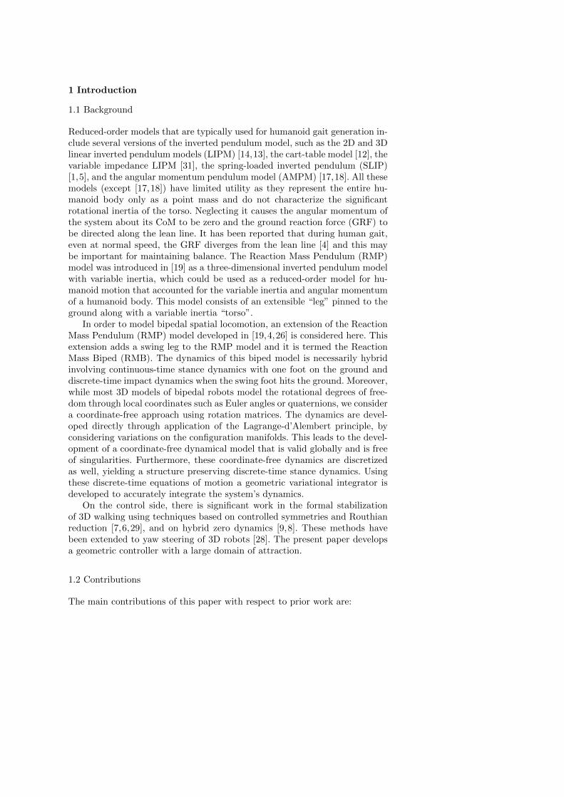
2.1 Physical description of the RMB Model

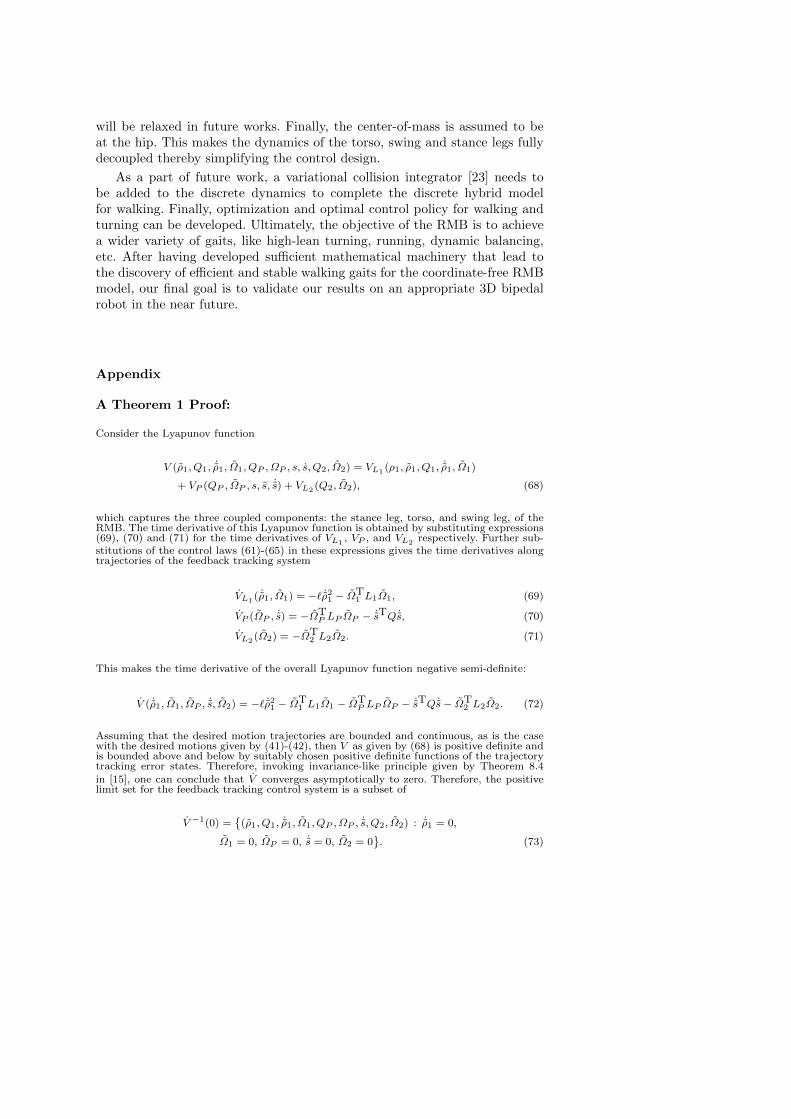
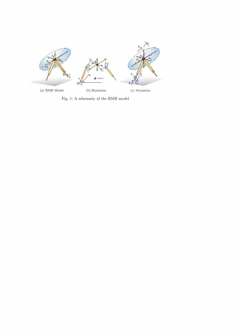
As shown in Fig.1(a), RMB consists of two extensible legs whose lengths areρ1 and ρ2 as measured from the RMB CoM (depicted by the quad-circle). TheCoM of both the legs is assumed to coincide with the RMB CoM. Moreover,forsome nominal length ρ0, the moment of inertia for the legs is given by JL0.The legs can extend up to a max distance r from ρ0. The torso is made upof three pairs(depicted in green) of reaction masses s1,s2,s3,respectively. Eachpair is arranged along an orthogonal axis ei of the torso’s body-fixed frame.With one each on either side of the RMB CoM , they are constrained to moveequidistantly so that the torso CoM always coincides with the RMB CoM.(b) The frames of reference used in this study are depicted here and they aredefined in Table 1. (c) We assume full actuation for the RMB model. τ1 rotatesthe ankle joint at the stance foot along pitch, roll and yaw directions w.r.t.the inertial frame I. f1 is the force used to extend the telescopic stance leg.τD1 ∈ R3 rotates torso frame P w.r.t the stance leg frame L1. Similarly,τD2 ∈ R3 rotates swing leg frame L2 w.r.t the torso frame P. Finally,us ∈ R3 actuates the reaction masses pairs on the torso. It is the motion ofthese point-masses that induces variability into the torso’s inertia.

2.2 Stance Dynamics (or) Fixed-base Robot Model

We develop a coordinate-free dynamic model for the stance phase of the Reac-tion Mass Biped, as shown in Fig. 1(a), by using rotation matrices to representthe attitudes of the two legs, R1, R2, and the torso, RP , along with scalarsρ1, ρ2 to represent the length of the two legs, and si to represent the positionof the ith pair of reaction masses. Note that, there are three pairs of reaction-masses, all of which are mutually orthogonal. During the stance phase, thestance-leg is assumed to be pinned to the ground. The Configuration Manifoldof the system is then given by Qs = C × SO(3) × SO(3) × SO(3) × S × C,

with ρ1, ρ2 ∈ C = [0, r], R1, RP , R2 ∈ SO(3), s =[s1 s2 s3

]T ∈ S =[0, rs]× [0, rs]× [0, rs]. The symbols used in this paper are tabulated in Table1.

We have the following kinematic relations in the system, R1 = R1Ω×1 ,

RP1 = RP1Ω×P1, RP = RPΩ

×P , R2P = R2PΩ

×2P , R2 = R2Ω

×2 , where,Ω1, Ω2, ΩP

are the respective body angular velocities, and are related by

ΩP = ΩP1 +RTP1Ω1, where, RP1 = R

T1 RP , (1)

Ω2 = Ω2P +RT2PΩP , where, R2P = R

TPR2. (2)

Here, the (.)× is called the hat operator and it is used to map angularvelocities from R3 to so(3) (the lie algebra of SO(3))Next, we derive an ex-pression for the kinetic energy of the system, Ts : TQs → R. We do this by firstfinding the position of the center-of-mass (COM) of the stance leg, b, and thepositions of the reaction mass pairs, pi±, in the inertial frame I as follows,

b = ρ1R1e3, pi± = b± siRP ei.

The dot product of their velocities can then be respectively computed as,

||b||2 = ρ21 − ρ21ΩT1 (e×3 )2Ω1 (3)

||pi+||2 + ||pi−||2 = 2(||b||2 + s2i − s2iΩP (e×i )2ΩP

), (4)

where (·)× : R3 → so(3) is the skew operator, defined such that x×y = x ×y,∀x, y ∈ R3. The kinetic energy of the system is then given by Ts = T1 +TP +T2, where, T1, T2 are the kinetic energies of the two legs respectively, andTP is the kinetic energy of the torso, computed as,

T1 =1

2mL||b||2 +

1

2ΩT1 JL0Ω1,

TP =1

2mP

(3∑i=1

||pi+||2 + ||pi−||2)

+1

2ΩTP JP0

ΩP ,

T2 =1

2mL||b||2 +

1

2ΩT2 JL0

Ω2.

Thus, the total kinetic energy of the system is,

Ts =1

2mρ21 +

3∑i=1

mP s2i +

1

2ΩT1 J1(ρ1)Ω1 +

1

2ΩTP JP (s)ΩP +

1

2ΩT2 JL0

Ω2, (5)

where,

J1(ρ1) = JL0 +K1(ρ1), K1(ρ1) = −mρ21(e×3 )2, m = 2mL + 6mP ,

JP (s) = JP0 +KP (s), KP (s) = −2∑3i=1mP s

2i (e×i )2.

Remark 1 Note that, the length of the swing leg, ρ2 does not appear in thekinetic energy of the system, and as we will consequently see, it will not appearin the dynamics either. This is because of representing COM of the swing legat the hip. Moving COM location to half-way along the leg will ensure theswing leg length velocity appears in the kinetic energy, thereby introducing anadditional dynamical equation for ρ2. The dynamical model and the controllerdeveloped here can easily be extended to incorporate a variable swing leglength, at the cost of adding another degree of freedom and some complexityto the dynamics. Here we treat the simpler case by assuming the swing leglength to be constant. The swing leg’s rotation does appear in the kineticenergy through Ω2.

Having developed an expression for the kinetic energy, we next computethe Potential Energy, Us : Qs → R, as,

Us = −mgρ1RT1 e3 · e3. (6)

Note that the negative sign arises due to our convention of e3 being along thegravitational direction.

The Lagrangian of the system Ls : TQs → R is then given by Ls =Ts−Us. The equations of motion can then be computed through the Lagrange-d’Alembert principle by writing the variation of the action integral as,

∫ (δLs + η1 · τ1 + δρ1f1 + ηP1 · τD1

3∑i=1

δsiusi + ηP2 · τD2

), (7)

where the first term in the integral represents the variation of the Lagrangian,computed using the following variations on SO(3),

δR1 = R1η×1 , η1 ∈ R3, δΩ1 = Ω×1 η1 + η1, (8)

δRP = RP η×P , ηP ∈ R3, δΩP = Ω×P ηP + ηP , (9)

δR2 = R2η×2 , η2 ∈ R3, δΩ2 = Ω×2 η2 + η2, (10)

and, all the other subsequent terms in the integral representing the infinitesi-mal virtual work, where,

ηP1 = ηP −RTPR1η1, ηP2 = η2 −RT2 RP ηP .

For more details and illustrations of the actuators, please refer to Fig. 1(c).The dynamical equations of motion can then be obtained by setting the aboveintegral to zero for all possible variations, resulting in,

mρ1 = −mρ1ΩT1 (e×3 )2Ω1 +mgeT3 RT1 e3 + f1, (11)

J1(ρ1)Ω1 = −Ω1 × J1(ρ1)Ω1 + 2mρ1ρ1(e×3 )2Ω1

+ mgρ1e×3 R

T1 e3 + τ1 −RT1 RP τD1

, (12)

JP (s)ΩP = −ΩP × JP (s)ΩP −N(s, s)ΩP

+ τD1−RTPR2τD2

, (13)

2mP s = −L(s,ΩP ) + us, (14)

JL0Ω2 = −Ω2 × JL0

Ω2 + τD2, (15)

where, N(s, s) =d

dtKP (s) = 4mP diag s2s2 + s3s3, s1s1 + s3s3, s1s1 + s2s2,

and, L(s,ΩP ) =∂

∂s(1

2ΩTP KP ΩP ) = 2mP

s1(Ω2P2

+Ω2P3

)s2(Ω2

P3+Ω2

P1)

s3(Ω2P1

+Ω2P2

)

.We can rewrite the above dynamical equations in a matrix form (use-

ful for the impact model) by defining qs =(ρ1, R1, RP , s, R2

), and ωs =[

ρ1 Ω1 ΩP s Ω2

]T. Thus, using qs,ωs, the equations of motion can be rewrit-

ten as

Ds(qs)ωs = Hs(qs,ωs) + Bsus,

where, Ds(qs) = diag (m,J1(ρ1), JP (s), 2mP I, JL0), and

Hs(qs,ωs) =

−mρ1ΩT1 (e×3 )2Ω1 +mgeT3 R

T1 e3

−Ω1 × J1(ρ1)Ω1 + 2mρ1ρ1(e×3 )2Ω1 +mgρ1e×3 R

T1 e3

−ΩP × JP (s)ΩP + 4∑3i=1mP sisi(e

×i )2ΩP

−L(s,ΩP )−Ω2 × JL0

Ω2

,

Bs(qs) =

I 0 0 0 00 I −RT1 RP 0 00 0 I 0 −RTPR2

0 0 0 I 00 0 0 0 I

,us =

f1τ1τD1

usτD2

.

Remark 2 Note that the stance dynamics of the Reaction Mass Biped is fullyactuated due to the ankle torque τ1 at the stance foot.

2.3 Extended Dynamics or Floating-base Robot Model

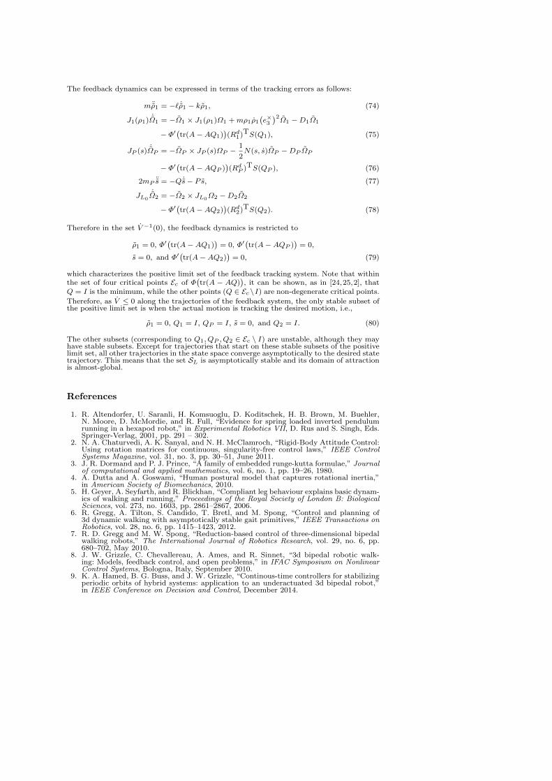
Having derived the stance dynamics of the Reaction Mass Biped system, wherethe stance leg is pinned to the ground, we now develop the extended model,where the foot is no longer pinned to the ground. This model is required toformulate the discrete-time impact model that captures the dynamics of swingfoot impact with the ground. The extended model is illustrated in Figure 2,and has the configuration manifold Qe = R3 × SO(3) × SO(3) × S × SO(3).The kinetic and potential energies, Te : TQe → R,Ue : Qe → R can be derivedin a similar manner as in the stance dynamics, resulting in,

Te =1

2mxP · xP +

3∑i=1

mP s2i +

1

2ΩT1 JL0Ω1

+1

2ΩTP JP (s)ΩP +

1

2ΩT2 JL0Ω2, (16)

Ue = −mgxP · e3. (17)

The dynamics of motion can be obtained through application of the Lagrange-d’Alembert principle as outlined earlier. We will directly write this in matrix

form by first defining, qe =(R1, RP , s, R2, xP

), and ωe =

[Ω1 ΩP s Ω2 xP

]T,

where xP is the position of the hip in the inertial frame. We then have,

De(qe)ωe = He(qe,ωe) + Be(qe)ue,

where, De(qe) = diag (JL0 , JP (s), 2mP I, JL0 ,m),

He(qe,ωe) =

−Ω1 × JL0Ω1

−ΩP × JP (s)ΩP + 4∑3i=1mP sisi(e

×i )2ΩP

−L(s,ΩP )−Ω2 × JL0

Ω2

mge3

, (18)

Be(qe) =

−RT1 RP 0 0

I 0 −RTPR2

0 I 00 0 I0 0 0

, ue =

τD1

usτD2

. (19)

Remark 3 Note that the extended dynamical model of the reaction mass bipedis under-actuated. This is in contrast to the stance dynamical model, which isfully actuated.

2.4 Impact Model

We will next develop the discrete-time impact model that captures the impactof the swing foot with the ground. The impact model results in an instanta-neous change in the joint velocities of the system. In order to capture this, we

will first need to map the stance coordinates to the extended coordinates, per-form the impact in the extended coordinates, map the extended coordinatesto the stance coordinates while accounting for the relabeling that occurs asthe old swing leg becomes the new stance leg.

First, to map the stance coordinates to the extended coordinates, we needto find xP , xP in terms of the stance coordinates. Since the stance foot is onthe ground, xP = ρ1R1e3. From this we obtain, xP = ρ1R1e3 + ρ1R1Ω

×1 e3.

We will write this as the following map,

qe = Υ qs→e(qs), ωe = Υω

s→e(ωs).

For later use, we will denote the map from the extended coordinates to thestance coordinates (assuming the first leg’s foot is in contact with the ground)as,

qs = Υ qe→s(qe), ωs = Υω

e→s(ωe).

This map essentially computes ρ1 from xP as, ρ1 = ||xP ||.Next we model the impact map. By considering (q−e ,ω

−e ) to be the state

prior to impact, and (q+e ,ω

+e ) to be the state post impact, and Fext represent-

ing the external force, we have the following relation from [10],

D(q+e )ω+

e −D(q−e )ω−e = Fext.

Further, the swing foot position and velocity are given as,

xF2= xP + ρtd2 R2e3, xF2

= xP − ρtd2 R2(e3)×Ω2,

where ρtd2 is the value of ρ2 at touchdown (note that ρtd2 is a constant and hasno dynamics since ρ2 can instantaneously change.) We require the post impactswing foot velocity x+F2

= 0, since this foot now becomes the new stance foot.This can be expressed as Aω+

e = 0, where,

A =[0 0 0− ρtd2 R+

2 (e3)× I].

Further, denoting IR as the impact force at the swing foot, we have Fext =AT IR. The above equations can then be expressed in matrix form to solve forω+e and IR, [

ω+e

IR

]=

[De(q

+e ) −AT

A 0

]−1 [−De(q−e )ω−e

0

]. (20)

We can then define a map Γ such that ω+e = Γ (ω−e ).

The impact map can then be defined by the map ∆s→s : S → TQ, whereS = xs ∈ TQs | (ρ2R2e3 − ρ1R1e3) · e3 = 0 is the switching surface repre-senting the contact of the swing leg toe with the ground. We have,

∆s→s :=

[∆qs→s

∆ωs→s

],

where, the components ∆qs→s and ∆ω

s→s define the transition maps for theconfiguration variables and their velocities, respectively. These are obtainedfrom the above equations as follows:

∆qs→s := Υ q

e→s R Υ qs→e,

∆ωs→s := Υω

e→s R Γ Υωs→e,

where R represents a coordinate relabeling transformation such that the oldswing leg is labeled as the new stance leg and vice-versa.

2.5 Hybrid System Model

The hybrid model for walking is based on the stance dynamics and the impactmodel developed in the previous sections, and can be represented as follows:

Σ :

Dsωs = Hs(qs,ωs) + Bs(qs)us, (q−s ,ω

−s ) /∈ S,

(q+s ,ω

+s ) = ∆s→s(q

−s ,ω

−s ), (q−s ,ω

−s ) ∈ S.

3 Discrete Mechanics and Variational Integrator for RMB

In general, for hybrid dynamical models like the RMB, conventional numericalintegrators, based on explicit Runge-Kutta method, are used for determiningthe system’s flow based on the continuous-time Euler-Lagrange equations thatwere derived in Section 2. However, this procedure results in the loss of somefundamental geometric properties of the system such as, inherent manifoldstructure, symplecticity, and the momentum map. Special integrators exist toeither preserve manifold structure of the configuration space [11,16] or sim-plecticity [22,33]. Recently, Lee et al [21,20] integrated these two techniquesand devised Geometric Variational Integrators (GVI) that are capable of pre-serving both geometry and structure of the discrete flow. In this section, wedevelop a discrete mechanics model of the RMB by taking variations of thecorresponding discrete action sum. The resulting update rules form the dis-crete equations of motion and they used to construct a GVI for the RMBsystem.

3.1 Discrete Lagrangian

The Lagrangian is discretized with a fixed step size, h ≥ 0, and the subscriptk determines the value at any iteration, as tk = kh. Therefore, the Configu-ration Manifold of the RMB at any time tk is given as Qs = C × SO(3) ×SO(3) × SO(3) × S × C, with configuration variables ρ1k , ρ2k ∈ C = [0, r],

R1k , RPk, R2k ∈ SO(3), sk =

[s1k s2k s3k

]T ∈ S.

For the discrete-time kinematic relations, the linear velocity xk at tk canbe approximated as shown

xk ≈∆xkh

=xk+1 − xk

h. (21)

Similarly, from the rotational kinematic relations in Section 2, the discreteanalogue of angular velocity is

Fk = ehΩ×k , so that Rk+1 = RkFk. (22)

Using (22) and (21), we get the following first order discrete equations for theRMB,

R1k+1= R1kF1k , RPk+1

= RPkFPk

, R2k+1= R2kF2k , (23)

ρ1k+1= ρ1k + hρ1k , sk+1 = sk + hsk, . (24)

The symbols specific to the Discrete Mechanics are tabulated in Table 2. Wederive the discrete versions of both kinetic (Ts) and potential (Us) energies ofthe system next. The discrete version of potential energy Usk : Qs → R is givenas Usk = −mgρ1keT3 RT1ke3, and the kinetic energy, defined as Tsk : TQs → R,is given as,

Tsk =1

2(mρ21k +

3∑i=1

mP s2ik

+ΩT1kJ1(ρ1k)Ω1k+

ΩTPkJP (sk)ΩPk

+ΩT2kJL0Ω2k). (25)

The discrete Lagrangian Lk approximates the path of least action, which isobtained by integrating the Lagrangian along the exact solution of the equa-tions of motion for a single time step,

Lk ≈∫ h

0

Ldt = L(ρ1k , sk, Ω1k , ΩPk, Ω2k)h = Tsk − Usk . (26)

Substituting (25) in (26) gives

Lk = h2 [ρ1k sk Ω1k ΩPk

Ω2k ]T

m

2mP IJ1(ρ1k)

JP (sk)JL0

ρ1kskΩ1k

ΩPk

Ω2k

+

hmgρ1keT3 R

T1ke3, (27)

where J1(ρ1k) = JL0−mρ21k(e×3 )2, JP (sk) = JP0−2∑3i=1mP s

2ik

(e×i )2. Similarto its continuous-time counterpart, the discrete-time version of the Lagrange-d’Alembert principle states that the action sum, which approximates the ac-tion integral, is invariant to the first order of all possible variations, as shown

in (28). Integrators that maintain this invariance are called Variational Inte-grators. Additionally, if they also maintain the structure of the configurationmanifold, they are called GVIs.

δSd =

N−1∑k=0

δLk + δWk = 0, where N =tF − t0h

. (28)

Here, t0, tF are the start and end times of the integration, respectively. Tocompute the above, we have to first determine the infinitesimal variations forRk and Ωk, as shown in [32],

δRk = limε→0

Rk exp (εη×k ) = Rkη×k , (29)

δFk = hδΩ×k exp (hΩ×k ) = hδΩ×k Fk, (30)

=⇒ δΩ×k =1

hδFkF

Tk =

1

h((Fkηk+1)× − η×k ),

∴ δΩk =1

h((Fkηk+1)− ηk). (31)

Additionally, the variations of ρ1k and sk are,

δ ˙ρ1k =δρ1k+1

− δρ1kh

, δsk =δsk+1 − δsk

h. (32)

The infinitesimal virtual work done and lagrangian can be discretized usingthe discrete infinitesimal variations obtained above as follows:

δWk = h(f1kδρ1k + uTskδsk + τT1kη1k + τTD1kηP1k + τTD2k

ηP2k),

δLk = h[ρ1k sk Ω1k ΩPkΩ2k ]T

m

2mP IJ1(ρ1k)

JP (sk)JL0

δρ1kδskδΩ1k

δΩPk

δΩ2k

−hmρ1kΩT1k(e×3 )2Ω1kδρ1k − h2mP

∑3i=1 sikΩ

TPk

(e×i )2ΩPkδsik

+hmgδρ1keT3 R

T1ke3 + hmgρ1ke

T3 δR

T1ke3. (33)

Now, we map all the velocities to their corresponding momentum terms andcontinue the rest of this derivation in terms of the momenta. Let, pρ1k = mρ1k ,psk = 2mP sk, Π1k = J1(ρ1k)Ω1k , ΠPk

= JP (sPk)ΩPk

, and Π2k = JL0Ω2k .

Accordingly, the discrete action sum in (28) can be rewritten using (33) as,

δSd =∑N−1k=0 [ΠT

1kδΩ1k +MT

k δR1k +ΠTPkδΩPk

+ΠT2kδΩ2k +

pρ1k (δρ1k+1− δρ1k)− hmρ1kΩT1k(e×3 )2Ω1kδρ1k +Nkδρ1k +∑3

i=1 psik (δsik+1− δsik)− h2mP sikΩ

TPk

(e×i )2ΩPkδsik + δWk] = 0.(34)

where, Mk =∂Usk∂R1k

and Nk =∂Usk∂ρ1k

. We can substitute (33), and the variations

(29),(31), and (32) in (34) to obtain the discrete action sum in terms of thevariations δυk := [η1k ηPk

η2k δρ1k δsk]. The fact that variations vanish atend points, i.e., δυk = 0 if k = 0, N , and an appropriate re-indexing of termsallows us to reformulate (34) as,

N−1∑k=1

[(FT1k−1Π1k−1

−Π1k +MTk R1k + hτ1k − hRP1kτD1k)T η1k

(FTPk−1ΠPk−1

−ΠPk+ hτD1k − hRP2kτD2k)T ηpk +

(FT2k−1Π2k−1

−Π2k + hτD2k)T η2k +

(pρ1k−1− pρ1k − hmρ1kΩ

T1k

(e×3 )2Ω1k +Nk + hf1k)δρ1k +

3∑i=1

(psik−1− psik − h2mP sikΩ

TPk

(e×i )2ΩPk+ huik)δsik ] = 0. (35)

Since (35) is true for any δυk, we require that the expressions each of in theparentheses to be equal to zero. They are indeed the discrete-time equations ofmotion for the RMB in terms of the momenta. Finally, we can map back fromthe momentum terms to the velocity terms to get the equations of motion interms of the velocities as shown below:

J1k+1Ω1k+1

= FT1k(J1kΩ1k) + hmgρ1k+1e×3 R

T1k+1

e3 + hτ1k+1− hRP1k+1

τD1k+1

(36)

JPk+1ΩPk+1

= FTPk(JPk

ΩPk) + hτD1k+1

− hRP2k+1τD2k+1

(37)

JL0Ω2k+1

= FT2k(JL0Ω2k) + hτD2k+1

(38)

mρ1k+1= mρ1k − hmρ1k+1

ΩT1k+1(e×3 )2Ω1k+1

+ hmgeT3 RT1k+1

e3 + hf1k+1

(39)

2mP sk+1 = 2mP sk − hL(sk+1, ΩPk+1) + huk+1 (40)

The discrete-time Lagrangian flow map takes us from (Ω1k ΩPkΩ2k ρ1k sk) 7→

(Ω1k+1ΩPk+1

Ω2k+1ρ1k+1

sk+1), and this process is repeated for N steps. Notethat, unlike in [21,20], this is an explicit method and doesn’t require customRodrigues formula-based gradient descent methods, and is therefore faster.

3.2 Advantages of Geometric Variational Integrators

1. GVIs preserve important mechanical properties like energy conservation(for conservative systems), momentum conservation (where there is sym-metry), while ensuring that the dynamics evolves in the configuration man-ifold of the system.

2. They can be easily implemented in hardware and the equations are inher-ently discrete-time.

3. This structure preserving property is also useful when building controllersbased on energy-like Lyapunov functions, as shown in this work.

4. Moreover, the performance does not degrade even for long simulation times.

4 Actuation and Controlled Motion

4.1 Motion Planning for Moving between Ground Locations

Consider a trajectory connecting two ground points with known initial andfinal velocities; there are many ways to generate this trajectory while avoidingfixed obstacles. The motion of the torso center of mass, when projected onthe horizontal (ground) plane, should closely follow this generated trajectory.Assuming that this trajectory is known a priori, a stride length that is optimal(or natural) for the RMB is used to determine the number of steps requiredto cover the path length. If ls is the optimal stride length and pl is the pathlength of the trajectory, then the nearest integer to pl/ls can be used as thenumber of strides required to cover this trajectory.

Desired trajectories (motion primitives) for variables associated with theRMB legs in time interval [0, T ] are:

ρd1 = ρ0 + ρ sin(ωt), ω =π

T, ρ0 > ρ > 0,

Rd1 = R10 exp(ζ×1 sin(ωt/2)

),

ρd2 = ρ0,

Rd2 = R20 exp(ζ×2 sin(ωt/2)

).

(41)

Note that the constant vectors ζ1, ζ2 ∈ R3 for the leg rotations could be equal,and something similar could be said for R10 , R20 ∈ SO(3) when the biped isstanding erect. Also, ρ0 and ρ are related to the optimal stride length for thebiped. The desired trajectories for variables associated with the torso over thetime interval [0, T ] are:

RdP = Rd1 exp(γ log

((Rd1)TRd2

)), γ ∈ [0, 1],

sd = s0 + s sin(ωt),(42)

where s0, s ∈ R3 are designed to have the appropriate inertia distribution forthe torso as mentioned earlier with |s0i| > |si|, log : SO(3) → so(3) is thelogarithm map that is inverse of the exponential map (given by the matrixexponential), and γ is a weight factor. Note that RdP = Rd1 when γ = 0 andRdP = Rd2 when γ = 1. The reasoning behind introducing these weights isto mimic human bipedal gait, where the body (torso) becomes more closelyaligned with the alignment of the stance leg as the speed of bipedal motionincreases. By making γ and ω time-varying, one can even transition between

different speeds of bipedal motion. This is one of the future goals of thisresearch.

The stride length is given by the horizontal distance traversed by the anklejoint of the swing leg in one cycle. The desired stride length can be obtainedfrom the above desired motions for the swing leg, considering that the inertialposition of the ankle/foot of the swing leg at an instant is given by

aL2 = aL1 + ρ1R1e3 − ρ2R2e3, (43)

where aL1, aL2 denote the positions of the ankles of the stance and swing leg,respectively. With the coordinate frames as illustrated in Fig. 1 and substi-tuting equation (41) for the desired motion trajectories, the starting and endpositions of the swing leg ankle during a cycle are:

asL2 = aL1 + ρ0R10e3 − ρ0R20e3,

aeL2 = aL1 + ρ0R10 exp(ζ×1 )e3 − ρ0R20 exp(ζ×2 )e3(44)

Therefore the stride length is given by

aeL2 − asL2 = ρ0R10

(exp(ζ×1 )− I

)e3 + ρ0R20

(I − exp(ζ×2 )

)e3. (45)

Using Rodrigues’ rotation formula, the above expression can be simplified to

vds = ρ0R10

ζ×1 sin ‖ζ1‖+

(ζ×1)2

(1− cos ‖ζ1‖)e3

− ρ0R20

ζ×2 sin ‖ζ2‖+

(ζ×2)2

(1− cos ‖ζ1‖)e3, (46)

where vds denotes the desired stride vector, and ζ1, ζ2 denote the unit vectorsalong ζ1, ζ2 respectively. This sets the desired stride length to lds = ‖vds‖.Note that the constraint eT

3 vds = 0 must be satisfied, which imposes certain

constraints on R10 , R20 , ζ1 and ζ2. Substituting (46) for vds , this constraint isexpressed as

ΓT10

ζ×1 sin ‖ζ1‖+

(ζ×1)2

(1− cos ‖ζ1‖)e3 =

ΓT20

ζ×2 sin ‖ζ2‖+

(ζ×2)2

(1− cos ‖ζ1‖)e3, (47)

where Γ10 = RT10e3, Γ20 = RT

20e3.

Expression (47) can be satisfied by setting

ζ1 = ζ2 and R20 = exp(θe×3 )R10 , (48)

for θ ∈ S1. The second equality in (48) guarantees that Γ10 = Γ20 ; physically,it means that the initial orientations of the stance and swing legs during startof a cycle are related by a rotation about the inertial third axis that pointsup. Substituting (48) in (42) to simplify the expression for RdP in (42), oneobtains:

(Rd1)TRd2 = exp(− c(t)ζ×1

)RT

10R20 exp(c(t)ζ×1

)= exp

(− c(t)ζ×1

)exp

(θ(RT

10e3)×)

exp(c(t)ζ×1

)= exp

(θ(

exp(−c(t)ζ×1 )RT10e3

)×)(49)

where c(t) = sin(ωt/2). The above simplification uses the following relationmultiple times:

RT exp(φe×)R = exp(φ(RTe)×

),

where e ∈ S2 is a unit vector. This leads to the following simplified expressionfor RdP :

RdP = Rd1 exp(γθ(

exp(−c(t)ζ×1 )RT10e3

)×), (50)

which can then be expanded using Rodrigues’ formula.

4.2 Trajectory Tracking Control Scheme

Define the trajectory tracking errors:

ρ1 = ρ1 − ρd1, ˙ρ1 =d

dtρ1,

Q1 = R1(Rd1)T, Ω1 = Ω1 −Ωd1 ,

QP = RP (RdP )T, ΩP = ΩP −ΩdP ,

s = s− sd, ˙s =d

dts,

Q2 = R2(Rd2)T, Ω2 = Ω2 −Ωd2 .

(51)

The trajectory tracking control scheme is a generalization of the control schemein [26]. The Lyapunov function candidate for the stance leg is:

VL1(ρ1, ρ1, Q1, ˙ρ1, Ω1) =

1

2m ˙ρ21 +

1

2ΩT

1 J1(ρ1)Ω1 +1

2kρ21

+ Φ(tr(A−AQ1)

), (52)

where k > 0, A = diag(a1, a2, a3) with a1 > a2 > a3 > 0, and Φ : R → R is aC2 function that satisfies Φ(0) = 0 and Φ′(x) > 0 for all x ∈ R+. Furthermore,let Φ′(·) ≤ α(·), where α(·) is a Class-K function [15]. The Lyapunov functioncandidate for the torso of the RMB is:

VP (QP , ΩP , s, s, ˙s) =1

2ΩTP JP (s)ΩP +mP

˙sT ˙s+1

2sTP s

+ Φ(tr(A−AQP )

). (53)

The Lyapunov function candidate for the swing leg is:

VL2(Q2, Ω2) =

1

2ΩT

2 JL0Ω2 + Φ

(tr(A−AQ2)

), (54)

where JL0is the inertia of swing leg at its nominal length (ρ0), which is kept

constant during swing phase, and P,Q1, QP , Q2 are suitable positive definitematrices that are use to build valid Lyapunov functions. The time derivativeof these Lyapunov functions along the stance dynamics of the RMB systemare evaluated next.

The time derivative of VL1 along dynamics (11)-(12) is:

d

dtVL1(ρ1, ρ1, Q1, ˙ρ1, Ω1) = ˙ρ1

[f1 −mρ1ΩT

1

(e×3)2Ω1

+mgeT3 Γ1 −mρd1 + kρ1

]+ ΩT

1

[−Ω1 × J1(ρ1)Ω1 + 2mρ1ρ1

(e×3)2Ω1 +mgρ1e

×3 Γ1

+ τ1 −RT1 RP τD1

− J1(ρ1)Ωd1 −mρ1ρ1(e×3)2Ω1

+ Φ′(tr(A−AQ1)

)(Rd1)TS(Q1)

], (55)

where Γ1 = RT1 e3 is the inertial z-axis direction (up) in the stance leg’s body-

fixed frame and S : SO(3)→ R3 is defined by

S(Q) =

3∑i=1

aiQTei × ei. (56)

After some partial cancellations of terms, this expression can be rewritten as

d

dtVL1

(ρ1, ρ1, Q1, ˙ρ1, Ω1) = ˙ρ1

[f1 −mρd1 −mρ1Ω1

(e×3)2Ω1 +mgeT

3 Γ1 + kρ1

]+ ΩT

1

[τ1 −RT

1 RP τD1−Ωd1 × J1(ρ1)Ω1 +mρ1ρ1

(e×3)2(

Ω1 +Ωd1)

+mgρ1e×3 Γ1 + Φ′

(tr(A−AQ1)

)(Rd1)TS(Q1)

]. (57)

The time derivative of VP along the dynamics (13)-(14) is:

d

dtVP (QP , ΩP , s, s, ˙s) = ΩT

P

[JP (s)ΩP ×ΩP + τD1

−N(s, s)ΩP −RTPR2τD2

− JP (s)ΩdP +1

2N(s, s)ΩP + Φ′

(tr(A−AQP )

)(RdP )TS(QP )

]+ ˙sT

[L(s,ΩP )− 2mP s

d + P s+ us

], (58)

where N(s, s) = ddtKP (s) and sTL(s,ΩP ) = 1

2ΩTPN(s, s)ΩP . After some par-

tial cancellation of terms, one can simplify expression (58) to

d

dtVP (QP , ΩP , s, s, ˙s) = ΩT

P

[τD1−RT

PR2τD2− JP (s)ΩdP −ΩdP × JP (s)ΩP

− 1

2N(s, s)

(ΩP +ΩdP

)+ Φ′

(tr(A−AQP )

)(RdP )TS(QP )

]+ ˙sT

[us + L(s,ΩP )− 2mP s

d + P s]. (59)

Finally, the time derivative of VL2along dynamics (15) is

d

dtVL2

(Q2, Ω2) =1

2ΩT

2

(−Ωd2 × JL0

Ω2 + τD2− JL0

Ωd2

+ Φ′(tr(A−AQ2)

)(Rd2)TS(Q2)

). (60)

Theorem 1 Let ` > 0 and let D1, DP , D2, P,Q ∈ R3×3 be positive definitematrices. Then the tracking control laws

f1 = mρd1 +mρ1ΩT1

(e×3)2Ω1 −mgeT

3 Γ1 − kρ1 − ` ˙ρ1, (61)

τ1 = RT1 RP τD1

+ J1(ρ1)Ωd1 +Ωd1 × J1(ρ1)Ω1 −mgρ1e×3 Γ1

−mρ1ρ1(e×3)2(

Ω1 +Ωd1)− Φ′

(tr(A−AQ1)

)(Rd1)TS(Q1)−D1Ω1, (62)

τD1= RT

PR2τD2+ΩdP × JP (s)ΩP + JP (s)ΩdP −DP ΩP

+1

2N(s, s)

(ΩP +ΩdP

)− Φ′

(tr(A−AQP )

)(RdP )TS(QP ), (63)

us = 2mP sd − L(s,ΩP )− P s−Q ˙s, (64)

τD2= Ωd2 × JL0

Ω2 + JL0Ωd2 −D2Ω2 − Φ′

(tr(A−AQ2)

)(Rd2)TS(Q2), (65)

asymptotically stabilize a desired state trajectory of the form given by equations(41)-(42). Further, the domain of convergence of this trajectory is almost globalin the state space in the absence of control constraints, disturbance forces anddisturbance torques.

Proof. See Appendix A.

Note that, this trajectory tracking control scheme can be applied in generalto track all C2 desired state trajectories, provided that actuator constraintsare not violated. In practice, the desired state trajectories can be designedkeeping in mind known actuator constraints for the RMB or for a humanoidrobot being modeled by the RMB.

5 Numerical Results

Having developed a geometric controller for asymptotically tracking trajecto-ries, we now validate the proposed controller through a numerical simulationof the hybrid model developed in Section 2.

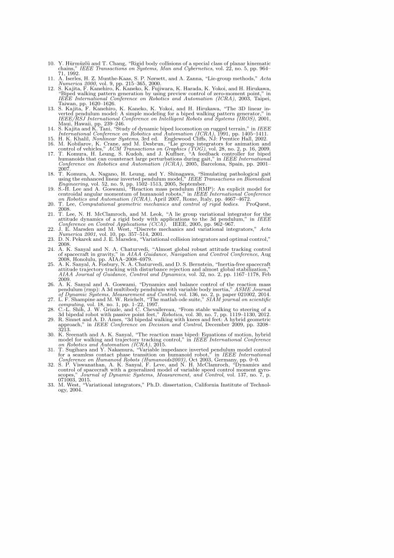
To illustrate the capability of the controller, we will demonstrate (a) walk-ing in a straight line, (b) walking towards a goal location, and (c) walking ina circle. In all cases, we choose a constant desired torso angle leaning forward,this is in contrast to (42) to simplify velocity and acceleration computation.The mass and inertia properties of the reaction mass biped are chosen to besimilar to that of a NAO robot, as done in [26], in particular,

mL = 0.882kg, JL0= 0.5diag0.98, 0.91, 0.63kg-m2,

mP = 0.32kg, JP0=

0.2126 0.0004 −0.00020.0004 0.2042 0.0010−0.0002 0.0010 0.2246

kg-m2.

Walking in a straight line: We chose ζ1 = ζ2 = e2, R10 = R20 = I, andT = 1s as in (41). Moreover, we introduce a constant phase offset in the anglesfor Rd1, R

d2 to enable the swing legs to swing from −15 to 15. For all other

motion design and controller gain parameters, see Table 3. Figure 3a illustratesa snapshot and the tracking errors.

Walking towards a goal: We employ the walking in a straight line controlleras above, however, we perform an event-based modification of R10, R20 at eachimpact to change the heading of the biped. Figure 3b illustrates a snapshot andthe tracking errors. Note that at each impact, the desired yaw instantaneouslychanges and the controller is able to regulate the errors asymptotically withina step.

Walking in a circle: We employ the walking towards a goal controller asabove, however we modify R10, R20 by a fixed amount at each impact. More-over, R10, R20 are also chosen to lean the body into the turn. Figure 3c illus-trates a snapshot (along with the hip position demonstrating the body lean)and the tracking errors. Note that instead of modifying R10, R20, we couldhave modified ζ1, ζ2 too.

For all these motions, it is important to verify that the unilateral groundcontact constraints and the friction constraints are satisfied during the walking,i.e., we need to ensure |Fx| ≤ µFz and |Fy| ≤ µFz, where µ is the coefficient ofstatic friction. The ground reaction forces were computed as, FG = mxcm −mge3, where FG := [Fx Fy Fz] and xcm is the center-of-mass of the RMB. It isequally critical to verify these constraints for the impact forces (IR in Section2.3) generated at the end of every step. Note that, the above-mentioned threemotions namely a) ’walking in a straight line’, b) ’walking towards a goal’ andc) ’walking in a circle’, take 10, 13, 19 steps respectively. In all these impactsituations, we note that IRz

is always positive (≥ 1.6019 N). Moreover, the

maximum values of|IRx |IRz

and|IRy |IRz

are 0.5872 and 0.5888, respectively, both

occurring while walking in a circle.

Combining the impact-force data with the stance leg ground reaction forceinformation, as shown in the third row of Fig. 3a, 3b, 3c, we can concludethat, for µ ≥ 0.6, the ground reaction force and the impact force respect theunilateral and friction cone constraints, thereby validating the assumptionsthat 1) stance leg is pinned to the ground during stance-phase and 2) No slipoccurs at impact.

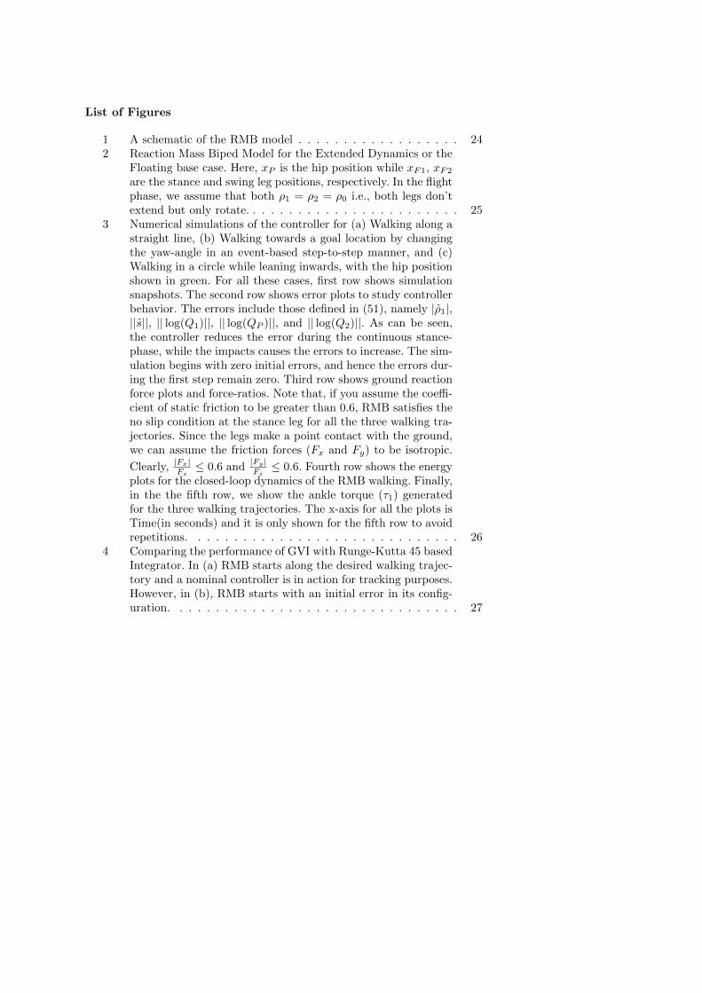
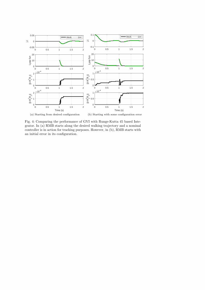
In addition to testing the trajectory tracking controller on the continuous-time dynamics model of the RMB, it was also tested on the Discrete-timemodel developed in Section 3. Figure 4 shows the performance of the GVIin comparison to the traditional Runge-Kutta(4,5)-based integrator (RK45).RK45 is a very popular numerical integration algorithm based on the explicitRunge-Kutta formula [3]. It is also part of Matlab’s ODE suite [27].

In Fig. 4(a), the two integrators are compared for a two-step walking sce-nario where the robot is initialized along the desired nominal trajectory(here,we chose the ’walking in a circle’ trajectory) given by (41) and (42): qs0 =(ρ0, R10 , RP0 , s0, R20). On the other hand, in 4(b), we start with a perturbedinitial conditions: qperts0 = (ρ0 + 0.1, Rx(π/10)R10 , RP0 , s0, R20) and ωperts0 =(ρ0, Ω10 , ΩP0

+0.01, s0−0.03, Ω20). Here Rx(θ) denotes a rotation along the x-direction by an angle θ. For both these cases, we plot (a) the desired leg exten-

sion tracking error (ρ) as obtained from (51) , (b) discrete Lyapunov function(obtained by discretizing (52), (53) and (54)) given by (66), and (c)-(d) R1, R2

norm errors. The norm errors are computed as ||I−RTi Ri|| ∀i ∈ 1, 2. If thegroup structure (R ∈ SO(3)) of R1 and R2 is preserved during the numericalintegrations, the norm errors must be closer to zero.

Vk(ρ1k , Q1k , ˙ρ1k , Ω1k , QPk, ΩPk

, sk, ˙sk, Q2k , Ω2k) = VL1k(ρ1k , ρ1k , Q1k , ˙ρ1k , Ω1k)

+ VPk(QPk

, ΩPk, sk, sk, ˙sk) + VL2k

(Q2k , Ω2k) (66)

where,

VL1k(ρ1k , ρ1k , Q1k , ˙ρ1k , Ω1k) =

1

2m ˙ρ21k +

1

2ΩT

1kJ1(ρ1k)Ω1k +

1

2kρ21k

+ Φ(tr(A−AQ1k)

),

VPk(QPk

, ΩPk, sk, sk, ˙sk) =

1

2ΩTPkJP (sk)ΩPk

+mP˙sTk

˙sk +1

2sTk P sk

+ Φ(tr(A−AQPk

)),

VL2k(Q2k , Ω2k) =

1

2ΩT

2kJL0

Ω2k + Φ(tr(A−AQ2k)

). (67)

Note that, for this study the step size chosen for the GVI and RK45 wash = 10−3. From the third and fourth rows of Fig.4, it is can be noted thatthe variational integrator maintained the group structure much better thanthe RK45 Integrator. On further examination, it was found that the GVIkept the norm error within 10−12 which is orders of magnitude better thanRK45. Moreover, other parameters like configuration errors(ρ), energies, etc.,as computed using the discrete GVI-based system model, track the continuousdynamics as accurately as the discrete-model based on RK45, if not better.

6 Conclusion and Future Work

A variable inertia multi-body reduced-order reaction mass biped model (RMB)is presented that can capture a much wider class of bipedal locomotion. Acoordinate-free hybrid dynamical model of the RMB is developed. A discreteversion of the model has also been developed that maintains the structuraland geometrical properties of the system and enables fast implementations onhardware. An asymptotically stable trajectory tracking control scheme withalmost global domain of convergence was also developed to enable the reactionmass biped to walk along straight and curved paths.

Despite all the useful additions, the RMB has room for improvement. Theinfluence of the reaction masses and the varying torso inertia on the gait designis not investigated. The primary objective of future work is to study the impactof upper-body inertia on RMB’s locomotory behavior. Additionally, the proofmasses are constrained to move together, either towards or away from eachother. We assume full actuation, but in reality there are under-actuated phases(toe-off) in walking which are not captured by this model. These constraints

will be relaxed in future works. Finally, the center-of-mass is assumed to beat the hip. This makes the dynamics of the torso, swing and stance legs fullydecoupled thereby simplifying the control design.

As a part of future work, a variational collision integrator [23] needs tobe added to the discrete dynamics to complete the discrete hybrid modelfor walking. Finally, optimization and optimal control policy for walking andturning can be developed. Ultimately, the objective of the RMB is to achievea wider variety of gaits, like high-lean turning, running, dynamic balancing,etc. After having developed sufficient mathematical machinery that lead tothe discovery of efficient and stable walking gaits for the coordinate-free RMBmodel, our final goal is to validate our results on an appropriate 3D bipedalrobot in the near future.

Appendix

A Theorem 1 Proof:

Consider the Lyapunov function

V (ρ1, Q1, ˙ρ1, Ω1, QP , ΩP , s, s, Q2, Ω2) = VL1(ρ1, ρ1, Q1, ˙ρ1, Ω1)

+ VP (QP , ΩP , s, s, ˙s) + VL2(Q2, Ω2), (68)

which captures the three coupled components: the stance leg, torso, and swing leg, of theRMB. The time derivative of this Lyapunov function is obtained by substituting expressions(69), (70) and (71) for the time derivatives of VL1

, VP , and VL2respectively. Further sub-

stitutions of the control laws (61)-(65) in these expressions gives the time derivatives alongtrajectories of the feedback tracking system

VL1( ˙ρ1, Ω1) = −` ˙ρ21 − ΩT

1 L1Ω1, (69)

VP (ΩP , ˙s) = −ΩTP LP ΩP − ˙sTQ ˙s, (70)

VL2 (Ω2) = −ΩT2 L2Ω2. (71)

This makes the time derivative of the overall Lyapunov function negative semi-definite:

V ( ˙ρ1, Ω1, ΩP , ˙s, Ω2) = −` ˙ρ21 − ΩT1 L1Ω1 − ΩT

P LP ΩP − ˙sTQ ˙s− ΩT2 L2Ω2. (72)

Assuming that the desired motion trajectories are bounded and continuous, as is the casewith the desired motions given by (41)-(42), then V as given by (68) is positive definite andis bounded above and below by suitably chosen positive definite functions of the trajectorytracking error states. Therefore, invoking invariance-like principle given by Theorem 8.4in [15], one can conclude that V converges asymptotically to zero. Therefore, the positivelimit set for the feedback tracking control system is a subset of

V −1(0) =

(ρ1, Q1, ˙ρ1, Ω1, QP , ΩP , ˙s,Q2, Ω2) : ˙ρ1 = 0,

Ω1 = 0, ΩP = 0, ˙s = 0, Ω2 = 0. (73)

The feedback dynamics can be expressed in terms of the tracking errors as follows:

m ¨ρ1 = −` ˙ρ1 − kρ1, (74)

J1(ρ1) ˙Ω1 = −Ω1 × J1(ρ1)Ω1 +mρ1ρ1(e×3

)2Ω1 −D1Ω1

− Φ′(tr(A−AQ1)

)(Rd1)TS(Q1), (75)

JP (s) ˙ΩP = −ΩP × JP (s)ΩP −1

2N(s, s)ΩP −DP ΩP

− Φ′(tr(A−AQP )

)(RdP )TS(QP ), (76)

2mP ¨s = −Q ˙s− P s, (77)

JL0

˙Ω2 = −Ω2 × JL0Ω2 −D2Ω2

− Φ′(tr(A−AQ2)

)(Rd2)TS(Q2). (78)

Therefore in the set V −1(0), the feedback dynamics is restricted to

ρ1 = 0, Φ′(tr(A−AQ1)

)= 0, Φ′

(tr(A−AQP )

)= 0,

s = 0, and Φ′(tr(A−AQ2)

)= 0, (79)

which characterizes the positive limit set of the feedback tracking system. Note that withinthe set of four critical points Ec of Φ

(tr(A − AQ)

), it can be shown, as in [24,25,2], that

Q = I is the minimum, while the other points (Q ∈ Ec\I) are non-degenerate critical points.

Therefore, as V ≤ 0 along the trajectories of the feedback system, the only stable subset ofthe positive limit set is when the actual motion is tracking the desired motion, i.e.,

ρ1 = 0, Q1 = I, QP = I, s = 0, and Q2 = I. (80)

The other subsets (corresponding to Q1, QP , Q2 ∈ Ec \ I) are unstable, although they mayhave stable subsets. Except for trajectories that start on these stable subsets of the positivelimit set, all other trajectories in the state space converge asymptotically to the desired statetrajectory. This means that the set SL is asymptotically stable and its domain of attractionis almost-global.

References

1. R. Altendorfer, U. Saranli, H. Komsuoglu, D. Koditschek, H. B. Brown, M. Buehler,N. Moore, D. McMordie, and R. Full, “Evidence for spring loaded inverted pendulumrunning in a hexapod robot,” in Experimental Robotics VII, D. Rus and S. Singh, Eds.Springer-Verlag, 2001, pp. 291 – 302.

2. N. A. Chaturvedi, A. K. Sanyal, and N. H. McClamroch, “Rigid-Body Attitude Control:Using rotation matrices for continuous, singularity-free control laws,” IEEE ControlSystems Magazine, vol. 31, no. 3, pp. 30–51, June 2011.

3. J. R. Dormand and P. J. Prince, “A family of embedded runge-kutta formulae,” Journalof computational and applied mathematics, vol. 6, no. 1, pp. 19–26, 1980.

4. A. Dutta and A. Goswami, “Human postural model that captures rotational inertia,”in American Society of Biomechanics, 2010.

5. H. Geyer, A. Seyfarth, and R. Blickhan, “Compliant leg behaviour explains basic dynam-ics of walking and running,” Proceedings of the Royal Society of London B: BiologicalSciences, vol. 273, no. 1603, pp. 2861–2867, 2006.

6. R. Gregg, A. Tilton, S. Candido, T. Bretl, and M. Spong, “Control and planning of3d dynamic walking with asymptotically stable gait primitives,” IEEE Transactions onRobotics, vol. 28, no. 6, pp. 1415–1423, 2012.

7. R. D. Gregg and M. W. Spong, “Reduction-based control of three-dimensional bipedalwalking robots,” The International Journal of Robotics Research, vol. 29, no. 6, pp.680–702, May 2010.

8. J. W. Grizzle, C. Chevallereau, A. Ames, and R. Sinnet, “3d bipedal robotic walk-ing: Models, feedback control, and open problems,” in IFAC Symposium on NonlinearControl Systems, Bologna, Italy, September 2010.

9. K. A. Hamed, B. G. Buss, and J. W. Grizzle, “Continous-time controllers for stabilizingperiodic orbits of hybrid systems: application to an underactuated 3d bipedal robot,”in IEEE Conference on Decision and Control, December 2014.

10. Y. Hurmuzlu and T. Chang, “Rigid body collisions of a special class of planar kinematicchains,” IEEE Transactions on Systems, Man and Cybernetics, vol. 22, no. 5, pp. 964–71, 1992.

11. A. Iserles, H. Z. Munthe-Kaas, S. P. Nørsett, and A. Zanna, “Lie-group methods,” ActaNumerica 2000, vol. 9, pp. 215–365, 2000.

12. S. Kajita, F. Kanehiro, K. Kaneko, K. Fujiwara, K. Harada, K. Yokoi, and H. Hirukawa,“Biped walking pattern generation by using preview control of zero-moment point,” inIEEE International Conference on Robotics and Automation (ICRA), 2003, Taipei,Taiwan, pp. 1620–1626.

13. S. Kajita, F. Kanehiro, K. Kaneko, K. Yokoi, and H. Hirukawa, “The 3D linear in-verted pendulum model: A simple modeling for a biped walking pattern generator,” inIEEE/RSJ International Conference on Intelligent Robots and Systems (IROS), 2001,Maui, Hawaii, pp. 239–246.

14. S. Kajita and K. Tani, “Study of dynamic biped locomotion on rugged terrain,” in IEEEInternational Conference on Robotics and Automation (ICRA), 1991, pp. 1405–1411.

15. H. K. Khalil, Nonlinear Systems, 3rd ed. Englewood Cliffs, NJ: Prentice Hall, 2002.16. M. Kobilarov, K. Crane, and M. Desbrun, “Lie group integrators for animation and

control of vehicles,” ACM Transactions on Graphics (TOG), vol. 28, no. 2, p. 16, 2009.17. T. Komura, H. Leung, S. Kudoh, and J. Kuffner, “A feedback controller for biped

humanoids that can counteract large perturbations during gait,” in IEEE InternationalConference on Robotics and Automation (ICRA), 2005, Barcelona, Spain, pp. 2001–2007.

18. T. Komura, A. Nagano, H. Leung, and Y. Shinagawa, “Simulating pathological gaitusing the enhanced linear inverted pendulum model,” IEEE Transactions on BiomedicalEngineering, vol. 52, no. 9, pp. 1502–1513, 2005, September.

19. S.-H. Lee and A. Goswami, “Reaction mass pendulum (RMP): An explicit model forcentroidal angular momentum of humanoid robots,” in IEEE International Conferenceon Robotics and Automation (ICRA), April 2007, Rome, Italy, pp. 4667–4672.

20. T. Lee, Computational geometric mechanics and control of rigid bodies. ProQuest,2008.

21. T. Lee, N. H. McClamroch, and M. Leok, “A lie group variational integrator for theattitude dynamics of a rigid body with applications to the 3d pendulum,” in IEEEConference on Control Applications (CCA). IEEE, 2005, pp. 962–967.

22. J. E. Marsden and M. West, “Discrete mechanics and variational integrators,” ActaNumerica 2001, vol. 10, pp. 357–514, 2001.

23. D. N. Pekarek and J. E. Marsden, “Variational collision integrators and optimal control,”2008.

24. A. K. Sanyal and N. A. Chaturvedi, “Almost global robust attitude tracking controlof spacecraft in gravity,” in AIAA Guidance, Navigation and Control Conference, Aug2008, Honolulu, pp. AIAA–2008–6979.

25. A. K. Sanyal, A. Fosbury, N. A. Chaturvedi, and D. S. Bernstein, “Inertia-free spacecraftattitude trajectory tracking with disturbance rejection and almost global stabilization,”AIAA Journal of Guidance, Control and Dynamics, vol. 32, no. 2, pp. 1167–1178, Feb2009.

26. A. K. Sanyal and A. Goswami, “Dynamics and balance control of the reaction masspendulum (rmp): A 3d multibody pendulum with variable body inertia,” ASME Journalof Dynamic Systems, Measurement and Control, vol. 136, no. 2, p. paper 021002, 2014.

27. L. F. Shampine and M. W. Reichelt, “The matlab ode suite,” SIAM journal on scientificcomputing, vol. 18, no. 1, pp. 1–22, 1997.

28. C.-L. Shih, J. W. Grizzle, and C. Chevallereau, “From stable walking to steering of a3d bipedal robot with passive point feet,” Robotica, vol. 30, no. 7, pp. 1119–1130, 2012.

29. R. Sinnet and A. D. Ames, “3d bipedal walking with knees and feet: A hybrid geometricapproach,” in IEEE Conference on Decision and Control, December 2009, pp. 3208–3213.

30. K. Sreenath and A. K. Sanyal, “The reaction mass biped: Equations of motion, hybridmodel for walking and trajectory tracking control,” in IEEE International Conferenceon Robotics and Automation (ICRA), 2015.

31. T. Sugihara and Y. Nakamura, “Variable impedance inverted pendulum model controlfor a seamless contact phase transition on humanoid robot,” in IEEE InternationalConference on Humanoid Robots (Humanoids2003), Oct 2003, Germany, pp. 0–0.

32. S. P. Viswanathan, A. K. Sanyal, F. Leve, and N. H. McClamroch, “Dynamics andcontrol of spacecraft with a generalized model of variable speed control moment gyro-scopes,” Journal of Dynamic Systems, Measurement, and Control, vol. 137, no. 7, p.071003, 2015.

33. M. West, “Variational integrators,” Ph.D. dissertation, California Institute of Technol-ogy, 2004.

List of Figures

1 A schematic of the RMB model . . . . . . . . . . . . . . . . . . 242 Reaction Mass Biped Model for the Extended Dynamics or the

Floating base case. Here, xP is the hip position while xF1, xF2

are the stance and swing leg positions, respectively. In the flightphase, we assume that both ρ1 = ρ2 = ρ0 i.e., both legs don’textend but only rotate. . . . . . . . . . . . . . . . . . . . . . . . 25

3 Numerical simulations of the controller for (a) Walking along astraight line, (b) Walking towards a goal location by changingthe yaw-angle in an event-based step-to-step manner, and (c)Walking in a circle while leaning inwards, with the hip positionshown in green. For all these cases, first row shows simulationsnapshots. The second row shows error plots to study controllerbehavior. The errors include those defined in (51), namely |ρ1|,||s||, || log(Q1)||, || log(QP )||, and || log(Q2)||. As can be seen,the controller reduces the error during the continuous stance-phase, while the impacts causes the errors to increase. The sim-ulation begins with zero initial errors, and hence the errors dur-ing the first step remain zero. Third row shows ground reactionforce plots and force-ratios. Note that, if you assume the coeffi-cient of static friction to be greater than 0.6, RMB satisfies theno slip condition at the stance leg for all the three walking tra-jectories. Since the legs make a point contact with the ground,we can assume the friction forces (Fx and Fy) to be isotropic.

Clearly, |Fx|Fz≤ 0.6 and

|Fy|Fz≤ 0.6. Fourth row shows the energy

plots for the closed-loop dynamics of the RMB walking. Finally,in the the fifth row, we show the ankle torque (τ1) generatedfor the three walking trajectories. The x-axis for all the plots isTime(in seconds) and it is only shown for the fifth row to avoidrepetitions. . . . . . . . . . . . . . . . . . . . . . . . . . . . . . 26

4 Comparing the performance of GVI with Runge-Kutta 45 basedIntegrator. In (a) RMB starts along the desired walking trajec-tory and a nominal controller is in action for tracking purposes.However, in (b), RMB starts with an initial error in its config-uration. . . . . . . . . . . . . . . . . . . . . . . . . . . . . . . . 27

(a) RMB Model (b) Rotations (c) Actuation

Fig. 1: A schematic of the RMB model

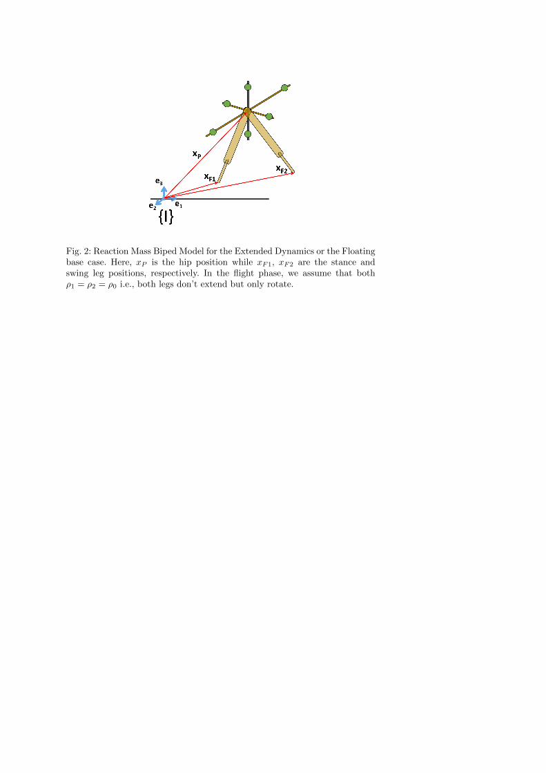
Fig. 2: Reaction Mass Biped Model for the Extended Dynamics or the Floatingbase case. Here, xP is the hip position while xF1, xF2 are the stance andswing leg positions, respectively. In the flight phase, we assume that bothρ1 = ρ2 = ρ0 i.e., both legs don’t extend but only rotate.

0

1

2

3

4

−2−1

01

2

0

0.5

1

1.5

2

2.5

3

YX

Z

0

1

2

3

4

−4−3

−2−1

01

0

0.5

1

1.5

2

2.5

3

YX

Z

−2

−1

0

1

2

−4−3

−2−1

01

0

0.5

1

1.5

2

2.5

3

YX

Z

0

0.02

0.04|ρ|||s||

0 5 10 150

0.1

0.2||log(Q1)||||log(QP )||||log(Q2)||

0

0.02

0.04|ρ|||s||

0 5 10 150

0.2

0.40

0.02

0.04|ρ|||s||

0 5 10 15 200

0.2

0.4

0

20

40

(N) |Fx|

|Fy|Fz

0 5 10 150

0.1

0.2

|Fx|/Fz

|Fy|/Fz

0

20

40

0 5 10 150

0.1

0.2

|Fx|/Fz

|Fy|/Fz

0

20

40

0 5 10 15 200

0.1

0.2

|Fx|/Fz

|Fy|/Fz

0 5 10 150

20

40

Ene

rgy(

J)

Kinetic

Potential

Total

0 5 10 150

20

40

0 5 10 15 200

20

40

0 5 10 15

Time(s)

-10

0

10

20

τ1 (

Nm

)

τx

τy

τz

(a) Walking Straight

0 5 10 15

Time(s)

-200

-100

0

100

(b) Walking to a Goal

0 5 10 15 20

Time(s)

-200

-100

0

100

(c) Walking in a Circle

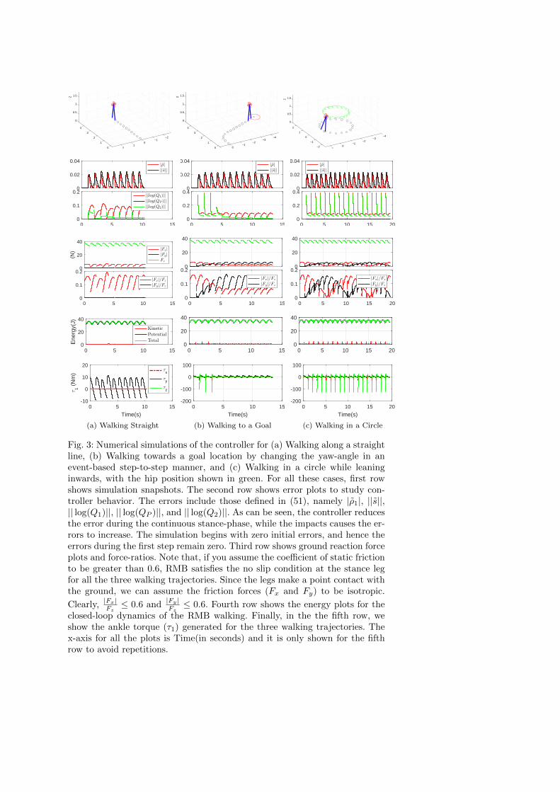
Fig. 3: Numerical simulations of the controller for (a) Walking along a straightline, (b) Walking towards a goal location by changing the yaw-angle in anevent-based step-to-step manner, and (c) Walking in a circle while leaninginwards, with the hip position shown in green. For all these cases, first rowshows simulation snapshots. The second row shows error plots to study con-troller behavior. The errors include those defined in (51), namely |ρ1|, ||s||,|| log(Q1)||, || log(QP )||, and || log(Q2)||. As can be seen, the controller reducesthe error during the continuous stance-phase, while the impacts causes the er-rors to increase. The simulation begins with zero initial errors, and hence theerrors during the first step remain zero. Third row shows ground reaction forceplots and force-ratios. Note that, if you assume the coefficient of static frictionto be greater than 0.6, RMB satisfies the no slip condition at the stance legfor all the three walking trajectories. Since the legs make a point contact withthe ground, we can assume the friction forces (Fx and Fy) to be isotropic.

Clearly, |Fx|Fz≤ 0.6 and

|Fy|Fz≤ 0.6. Fourth row shows the energy plots for the

closed-loop dynamics of the RMB walking. Finally, in the the fifth row, weshow the ankle torque (τ1) generated for the three walking trajectories. Thex-axis for all the plots is Time(in seconds) and it is only shown for the fifthrow to avoid repetitions.

0 0.5 1 1.5 2-0.05

0

0.05

|ρ|

RK45 GVI

0 0.5 1 1.5 20

10

20

Lyap

fun

0 0.5 1 1.5 20

1

2

||I-R

1TR

1||

×10-4

0 0.5 1 1.5 2

Time (s)

0

1

2

||I-R

2TR

2||

×10-4

(a) Starting from desired configuration

0 0.5 1 1.5 2-0.1

0

0.1

|ρ|

RK45 GVI

0 0.5 1 1.5 20

10

20

Lyap

fun

0 0.5 1 1.5 20

0.5

1

||I-R

1TR

1||

×10-4

0 0.5 1 1.5 2

Time (s)

0

0.5

1

||I-R

2TR

2||

×10-4

(b) Starting with some configuration error

Fig. 4: Comparing the performance of GVI with Runge-Kutta 45 based Inte-grator. In (a) RMB starts along the desired walking trajectory and a nominalcontroller is in action for tracking purposes. However, in (b), RMB starts withan initial error in its configuration.

List of Tables

1 Enumeration of the symbolic notation used in the paper. . . . . 292 Notations used in the discrete mechanics of RMB . . . . . . . . 303 List of various tuning parameters used in the Motion Primitive

and Controller designs. . . . . . . . . . . . . . . . . . . . . . . . 31

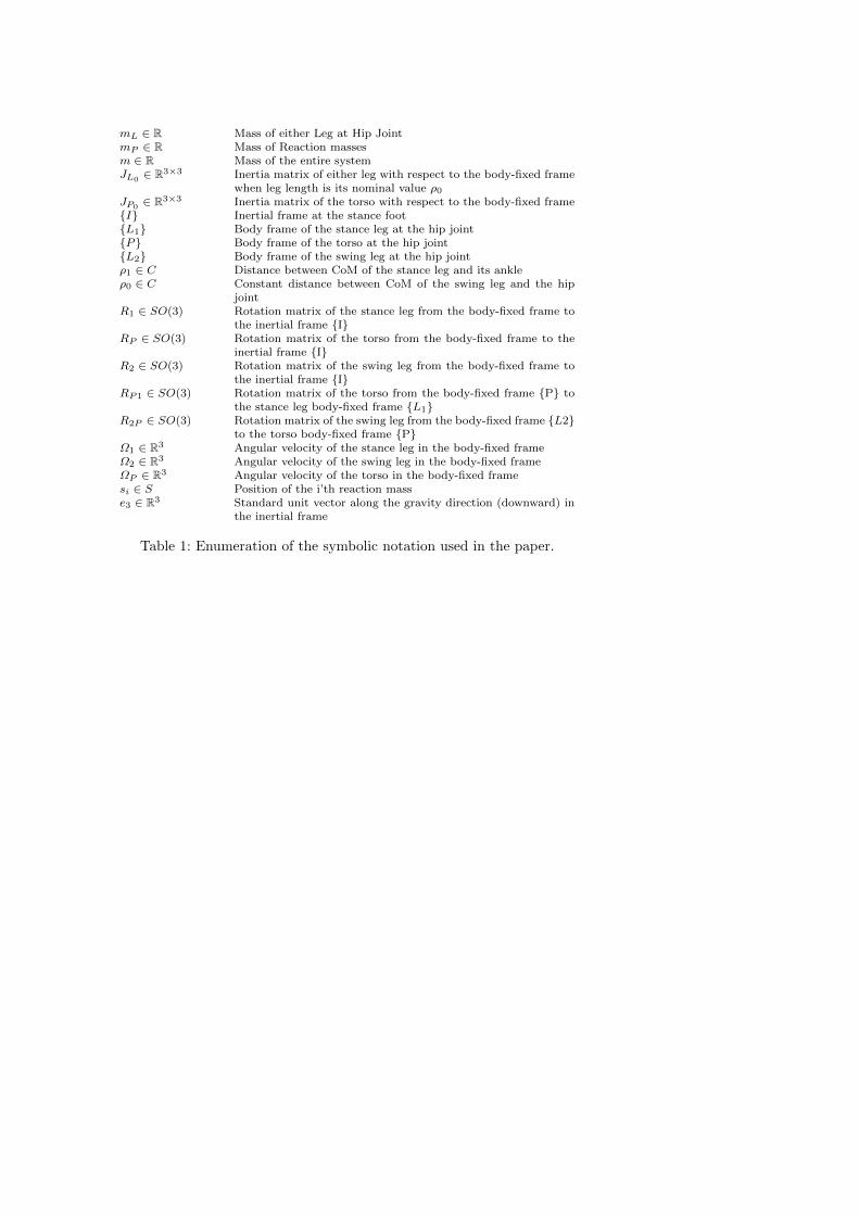
mL ∈ R Mass of either Leg at Hip JointmP ∈ R Mass of Reaction massesm ∈ R Mass of the entire systemJL0∈ R3×3 Inertia matrix of either leg with respect to the body-fixed frame

when leg length is its nominal value ρ0JP0∈ R3×3 Inertia matrix of the torso with respect to the body-fixed frame

I Inertial frame at the stance footL1 Body frame of the stance leg at the hip jointP Body frame of the torso at the hip jointL2 Body frame of the swing leg at the hip jointρ1 ∈ C Distance between CoM of the stance leg and its ankleρ0 ∈ C Constant distance between CoM of the swing leg and the hip

jointR1 ∈ SO(3) Rotation matrix of the stance leg from the body-fixed frame to

the inertial frame IRP ∈ SO(3) Rotation matrix of the torso from the body-fixed frame to the

inertial frame IR2 ∈ SO(3) Rotation matrix of the swing leg from the body-fixed frame to

the inertial frame IRP1 ∈ SO(3) Rotation matrix of the torso from the body-fixed frame P to

the stance leg body-fixed frame L1R2P ∈ SO(3) Rotation matrix of the swing leg from the body-fixed frame L2

to the torso body-fixed frame PΩ1 ∈ R3 Angular velocity of the stance leg in the body-fixed frameΩ2 ∈ R3 Angular velocity of the swing leg in the body-fixed frameΩP ∈ R3 Angular velocity of the torso in the body-fixed framesi ∈ S Position of the i’th reaction masse3 ∈ R3 Standard unit vector along the gravity direction (downward) in

the inertial frame

Table 1: Enumeration of the symbolic notation used in the paper.

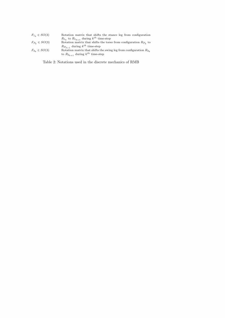
F1k ∈ SO(3) Rotation matrix that shifts the stance leg from configurationR1k to R1k+1

during kth time-stepFPk

∈ SO(3) Rotation matrix that shifts the torso from configuration RPkto

RPk+1during kth time-step

F2k ∈ SO(3) Rotation matrix that shifts the swing leg from configuration R2k

to R2k+1during kth time-step

Table 2: Notations used in the discrete mechanics of RMB

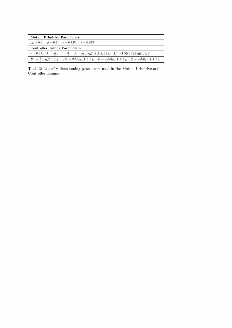
Motion Primitive Parameters

ρ0 = 0.9, ρ = 0.1, s = 0.125, s = 0.025.

Controller Tuning Parameters

ε = 0.25, k = 16ε2, l = 8

ε, A = 1

ε2diag(1.2, 1.5, 1.8), L = (1.5)(1.2)diag(1, 1, 1),

D1 = 2εdiag(1, 1, 1), D2 = 0.5

εdiag(1, 1, 1), P = 1.2

ε2diag(1, 1, 1), Q = 1.5

εdiag(1, 1, 1).

Table 3: List of various tuning parameters used in the Motion Primitive andController designs.