![[04899] - Design of Pile & Pile-Cap](https://static.fdocuments.net/doc/165x107/5695d3331a28ab9b029d273d/04899-design-of-pile-pile-cap.jpg)


Languages
Pages
Legal


Munich Personal RePEc Archive
The ‘Pile-up Problem’ in Trend-Cycle
Decomposition of Real GDP: Classical
and Bayesian Perspectives
Kim, Chang-Jin and Kim, Jaeho
University of WAshington and Korea University, University of
Washington
October 2013
Online at https://mpra.ub.uni-muenchen.de/51118/
MPRA Paper No. 51118, posted 12 Nov 2013 06:37 UTC

The ‘Pile-up Problem’ in Trend-Cycle Decomposition of Real GDP:Classical and Bayesian Perspectives
by
Chang-Jin KimUniversity of Washington and Korea University
andJaeho Kim 1
University of Washington
Preliminary DraftOctober 29, 2013
Abstract
In the case of a flat prior, a conventional wisdom is that Bayesian inference may notbe very different from classical inference, as the likelihood dominates the posterior density.This paper shows that there are cases in which this conventional wisdom does not apply.An ARMA model of real GDP growth estimated by Perron and Wada (2009) is an example.While their maximum likelihood estimation of the model implies that real GDP may be atrend stationary process, Bayesian estimation of the same model implies that most of thevariations in real GDP can be explained by the stochastic trend component, as in Nelson andPlosser (1982) and Morley et al. (2003). We show such dramatically different results stemfrom the differences in how the nuisance parameters are handled between the two approaches,especially when the parameter estimate of interest is dependent upon the estimates of thenuisance parameters for small samples.
For the maximum likelihood approach, as the number of the nuisance parameters in-creases, we have higher probability that the moving-average root may be estimated to beone even when its true value is less than one, spuriously indicating that the data is ‘over-differenced.’ However, the Bayesian approach is relatively free from this pile-up problem, asthe posterior distribution is not dependent upon the nuisance parameters.
1 Chang-Jin Kim: Dept. of Economics, University of Washington, Seattle, WA andDept. of Economics, Korea University, Seoul, Korea (E-mail: [email protected]);Jaeho Kim: Department of Economics, University of Washington, Seattle, WA. (E-mail:[email protected]). Chang-Jin Kim acknowledges financial support from the BryanC. Cressey Professorship at the University of Washington. Jaeho Kim acknowledges financialsupport from the Grover and Creta Ensley Fellowship in Economic Policy at the Universityof Washington. We thank the Charles R. Nelson, Richard Startz, and Eric Zivot for helpfulcomments.
1
1. Introduction
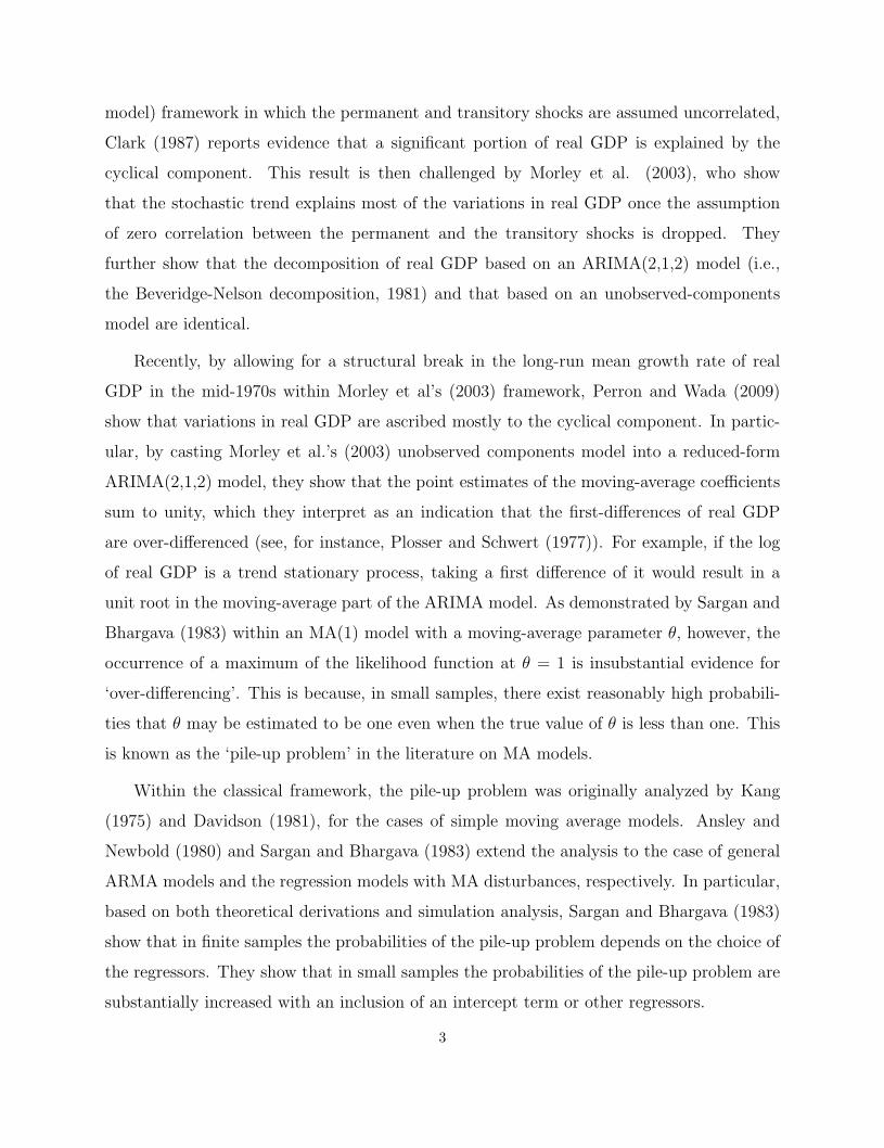
Since the seminal work of Nelson and Plosser (1982), one of the important issues in
empirical macroeconomics has been to investigate the degree of persistence in real economic
activities or the relative importance of permanent and transitory shocks. This issue has been
investigated in two directions. One strand of research is based on the unit root implication
of real GDP and the other is based on a direct measure of the relative sizes of the stochastic
trend and cyclical components of real GDP. In both strands of research, researchers provide
conflicting evidence on the existence of a unit root or the relative sizes of the stochastic trend
and the cyclical components in real GDP.
For example, while Nelson and Plosser (1982) report a unit root for real GDP as well
as for most of the macroeconomic variables they considered, Perron (1989) argues that,
by allowing for the possibility of a structural break (with known break date) in the trend
function of real GDP, the null hypothesis of a unit root can be rejected. This result was
criticized by Christiano (1992) and Zivot and Andrews (1992), who argue that the unit root
can no longer be rejected once one incorporates uncertainty about the date of a structural
break in the trend function. Cheung and Chinn (1997) apply both the unit root test and the
stationarity test to post-war real GDP and find that neither test rejects the null hypothesis.
They argue that the power of both tests is so low that no unambiguous conclusions can be
made. That is, as also suggested by DeJong et al. (1992), the inferences based exclusively
on tests for integration may be fragile. 2
Concerning the second strand of research, in which researchers are interested in the
relative sizes of the stochastic trend and the cyclical components, researchers also report
conflicting results. Based on estimation of ARMA models for real output growth, Nelson
and Plosser (1982) and Campbell and Mankiw (1987) conclude that transitory shocks are
relatively unimportant in explaining the dynamics of real output, while permanent shocks
must dominate. On the contrary, within an unobserved-components model (hereafter, UC
2 Furthermore, as surveyed by Murray and Nelson (2002), researchers who employ a longtime series that goes back to 1870, Diebold and Senhadji (1996), Cheung and Chinn (1997),Murray and Nelson (2000, 2002), and Newbold, Leyboure, and Wohar (2001) produce mixedconclusions. Their results differ depending on how the period around the Great Depression.
2
model) framework in which the permanent and transitory shocks are assumed uncorrelated,
Clark (1987) reports evidence that a significant portion of real GDP is explained by the
cyclical component. This result is then challenged by Morley et al. (2003), who show
that the stochastic trend explains most of the variations in real GDP once the assumption
of zero correlation between the permanent and the transitory shocks is dropped. They
further show that the decomposition of real GDP based on an ARIMA(2,1,2) model (i.e.,
the Beveridge-Nelson decomposition, 1981) and that based on an unobserved-components
model are identical.
Recently, by allowing for a structural break in the long-run mean growth rate of real
GDP in the mid-1970s within Morley et al’s (2003) framework, Perron and Wada (2009)
show that variations in real GDP are ascribed mostly to the cyclical component. In partic-
ular, by casting Morley et al.’s (2003) unobserved components model into a reduced-form
ARIMA(2,1,2) model, they show that the point estimates of the moving-average coefficients
sum to unity, which they interpret as an indication that the first-differences of real GDP
are over-differenced (see, for instance, Plosser and Schwert (1977)). For example, if the log
of real GDP is a trend stationary process, taking a first difference of it would result in a
unit root in the moving-average part of the ARIMA model. As demonstrated by Sargan and
Bhargava (1983) within an MA(1) model with a moving-average parameter θ, however, the
occurrence of a maximum of the likelihood function at θ = 1 is insubstantial evidence for
‘over-differencing’. This is because, in small samples, there exist reasonably high probabili-
ties that θ may be estimated to be one even when the true value of θ is less than one. This
is known as the ‘pile-up problem’ in the literature on MA models.
Within the classical framework, the pile-up problem was originally analyzed by Kang
(1975) and Davidson (1981), for the cases of simple moving average models. Ansley and
Newbold (1980) and Sargan and Bhargava (1983) extend the analysis to the case of general
ARMA models and the regression models with MA disturbances, respectively. In particular,
based on both theoretical derivations and simulation analysis, Sargan and Bhargava (1983)
show that in finite samples the probabilities of the pile-up problem depends on the choice of
the regressors. They show that in small samples the probabilities of the pile-up problem are
substantially increased with an inclusion of an intercept term or other regressors.
3
Within the Bayesian framework, however, the nature of the pile-up problem has not been
fully investigated. For an MA(1) model without an intercept term, DeJong and Whiteman
(1993) show that, while the sampling distributions of the maximum likelihood estimator of
θ (θML) piles up at unity when the true parameter is near unity, the (Bayesian) flat-prior
posterior distributions of θ do not pile up regardless of the parameter’s proximity to unity.
They also show that posterior distributions of peak at the maximum likelihood estimates.
These are illustrated by comparing the sampling distribution of θML and the posterior dis-
tribution of θ, which are obtained from the joint distribution of θML and θ constructed based
on Monte Carlo simulations. These results are taken by DeJong and Whiteman (1993) as a
rationale for favoring the Bayesian approach over the classical approach. 3
In this paper, we estimate Perron and Wada’s (2009) model by applying the Bayesian
approach. 4 Surprisingly, the trend-cycle decomposition of real GDP implied by the Bayesian
parameter estimates turn out to be very different from that implied by Perron and Wada’s
(2009) maximum likelihood estimates, even with reasonably non-informative priors. That
is, most of the variations in real GDP can be explained by the stochastic trend component,
consistent with the implications of Nelson and Plosser (1982) and Morley et al. (2003).
Unlike the predictions of DeJong and Whiteman (1993), the posterior mode for the sum of
moving-average parameters do not peak at its maximum likelihood estimate of one. Instead,
the posterior mode is close to the local maximum of the likelihood function in the invertible
region, even though there exists a non-negligible probability mass near the non-invertible
boundary of one.
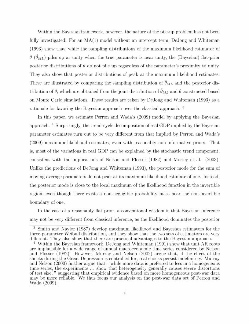
In the case of a reasonably flat prior, a conventional wisdom is that Bayesian inference
may not be very different from classical inference, as the likelihood dominates the posterior
3 Smith and Naylor (1987) develop maximum likelihood and Bayesian estimators for thethree-parameter Weibull distribution, and they show that the two sets of estimators are verydifferent. They also show that there are practical advantages to the Bayesian approach.
4 Within the Bayesian framework, DeJong and Whiteman (1991) show that unit AR rootsare implausible for a wide range of annual macroeconomic time series considered by Nelsonand Plosser (1982). However, Murray and Nelson (2002) argue that, if the effect of theshocks during the Great Depression is controlled for, real shocks persist indefinitely. Murrayand Nelson (2000) further argue that, “while more data is preferred to less in a homogeneoustime series, the experiments ... show that heterogeneity generally causes severe distortionsof test size, ” suggesting that empirical evidence based on more homogeneous post-war datamay be more reliable. We thus focus our analysis on the post-war data set of Perron andWada (2009).
4

density. This paper confirms that the ARMA model of real GDP estimated by Perron
and Wada (2009) is an example in which this conventional wisdom does not apply. We
show such dramatically different results based on the maximum likelihood and the Bayesian
approaches stem from the differences in how the nuisance parameters are handled between
the two approaches, especially when the parameter estimate of interest is dependent upon
the estimates of the nuisance parameters for small samples. For the maximum likelihood
approach, as the number of the nuisance parameters increases, we have higher probability
that the moving-average root may be estimated to be one even when its true value is less than
one, spuriously indicating that the data is over-differenced. However, the Bayesian approach
is relatively free from this pile-up problem, as the posterior distribution is not dependent
upon the nuisance parameters.
We also apply the Bayesian approach to an ARIMA(2,1,2) model for the log of real GDP,
by relaxing the assumption of a known break date for the mean growth rate. A reduction
in the variance of the shocks to real GDP, namely the Great Moderation (Kim and Nelson
(1999) and McConnell and Perez-Quiros (2000)), is also incorporated. Our results suggest
that the posterior mean and mode of θ1 + θ2 are 0.137 and 0.427, respectively, which are
further away from unity than in the case of a known structural break date. However, the
probability mass at unity almost disappears for the posterior distribution, unlike in the case
of known break dates. This suggests that, with the inclusion of the break date uncertainty,
we have even less probability of post-war U.S. real GDP being a trend stationary process than
in the case of a known break date. Furthermore, the implied cyclical component is noisy and
small in magnitude, with most variations in real GDP being explained by the stochastic trend
component. That is, even after taking breaks with uncertain break dates, the implications of
Nelson and Plosser (1982) and Morley et al. (2003) on trend-cycle decomposition continue
to hold within the Bayesian framework, which is relatively free from the pile-up problem.
The paper is organized as follows. In Section 2, we show that results from Bayesian
estimation of Perron and Wada’s (2009) model are very different from those from maximum
likelihood estimation. In Section 3, we discuss the nature of the classical pile-up problem,
and present a simulation study showing that Perron and Wada’s (2009) results may be due
to the classical pile-up problem. In Section 4, we provide an answer to the question of why
5

the results from the classical and Bayesian approaches are so different. In particular, we
provide a discussion of why the Bayesian approach may be relatively free from the pile-up
problem. In Section 5, we apply the Bayesian approach to an extended ARIMA(2,1,2) model
of real GDP, in which we incorporate a structural break in the variance of shocks (Great
moderation) and in the long-run mean growth rate with uncertain break dates. Section 6
concludes the paper.
2. Preliminaries: Classical and Bayesian Perspectives for Trend-Cycle Decom-position of Real GDP [1947:I - 1998:II]
Harvey (1985), Clark (1987), and Morley et al. (2003), among others, consider the
following unobserved components model of real GDP:
yt = xt + zt,
xt = µt + xt−1 + vt (1)
φ(L)zt = ǫt
[
vt
ǫt
]
∼ i.i.d.N
[
σ2v
ρσǫσv
ρσvσǫ
σ2ǫ
]
,
where yt is the log of real GDP; xt is a stochastic trend component; and zt is a cyclical
component with all the roots of φ(L) = 0 lying outside the complex unit circle.
Literature suggests that different assumptions about the dynamics of the long-run mean
growth rate µt or a restriction on the correlation coefficient ρ can lead to different trend-
cycle decompositions. For example, with a zero restriction on the ρ parameter and a random
walk specification for µt, Clark (1987) estimates the cyclical component (zt) to be highly
persistent and shows that a significant portion of real GDP is explained by this component.
By assuming that µt is constant and allowing for a possibility that ρ may be non-zero, Morley
et. al (2003) estimates the cyclical component to be noisy and considerably smaller than that
in Clark (1987). On the contrary, by modeling µt as a constant interrupted by a permanent
change occurring in 1973:I, Perron and Wada (2009) estimate the variance of the permanent
shocks σ2v to be zero, suggesting that real GDP is a trend stationary process.
6

As Morley et al. (2003) present, one potential difficulty in estimating the above unob-
served components model is that it is identified only when zt is autoregressive of order higher
than one. Furthermore, when they estimate the model with an AR(2) dynamics for zt, they
show that the confidence intervals for the ρ parameter are so large that various trend-cycle
decompositions are possible depending on which value of the ρ parameter is chosen within
the confidence interval. As they suggest, one way to overcome these difficulties is to esti-
mate a reduced-form ARIMA model for real GDP and employ the Beveridge-Nelson (1981)
decomposition procedure. For example, if we assume that φ(L) = 1 − φ1L − φ2L2 and µt is
a constant with a permanent shift in 1973:I, a reduced-form ARIMA model considered by
Perron and Wada (2009) is given by:
Perron and Wada’s (2009) Model
∆yt = µ0 + µ1Dt + ∆y∗
t ,
∆y∗
t = φ1∆y∗
t−1 + φ2∆y∗
t−2 + et − θ1et−1 − θ2et−2, (2)
Dt = 0 for t ≤ 1973 : I; and Dt = 1, otherwise.
et ∼ i.i.d.N(0, σ2e),
where σ2e and the moving-average parameters θ1 and θ2 are functions of φ1, φ2, σ2
v , σ2ǫ , and
ρ.
It is easy to show that a unit root in the moving average part of the above ARIMA model
is equivalent to the case of σ2v = 0 in the UC model of (1). In this case ∆yt is over-differenced,
and yt is a trend stationary process. Perron and Wada (2009) estimate the above ARIMA
model as well, and report that the maximum likelihood estimates of the moving-average
parameters sum to unity, which is consistent with their estimate of σ2v = 0 for the UC model
in (1). We replicate Perron and Wada’s (2009) results by employing the same model in (2)
and data set (quarterly real GDP, 1947:I to 1998:II) as used by them. 5 Table 1 reports the
results, from which we note that a local maximum exists within the invertibility region of
the moving average parameters as well as the global maximum at θ1 + θ2 = 1.
5 This data set was originally used in Morley et al. (2003).
7

In this section, we consider Bayesian inference of the model in (2) and the results are
compared to those based on classical inference by Perron and Wada (2009). In the case
of a flat prior, a conventional wisdom is that Bayesian inference may not be very different
from classical inference, as the likelihood dominates the posterior density. In Table 2, the
posterior moments of the parameters are presented. Surprisingly, estimation results based on
the Bayesian approach with reasonably non-informative priors are very different from those
based on the maximum likelihood method. The posterior mean and the posterior mode of
θ1 + θ2 turn out to be 0.286 and 0.498, respectively, as opposed to its maximum likelihood
estimate of unity. An interesting finding is that the parameter values at the posterior modes
are very close to those at the local maximum of the log likelihood function. However, from
the posterior distribution of θ1 +θ2 depicted in Figure 1.A, we cannot rule out the possibility
that θ1 +θ2 = 1, as there exists a non-negligible probability mass at unity. 6 The probability
is about 5%.
At each iteration of the Markov Chain Monte Carlo (MCMC), we apply the Beveridge-
Nelson (1981) decomposition procedure to get the cyclical component of real GDP. In Figure
1.B, the estimates of the cyclical component from this procedure and that implied by Perron
and Wada’s (2009) maximum likelihood estimation are compared. The corresponding trend
components are also depicted against the log of the real GDP series. While variations in real
GDP are explained mostly by the cyclical components within the classical framework, they
are explained mostly by the stochastic trend component within the Bayesian framework. The
impulse-response functions (∂yt+j
∂et)) depicted in Figure 1.B further confirm this point. Within
the Bayesian framework, the posterior mode of the long-run impulse-response coefficient
(limj→∞
∂yt+j
∂et) is 1.359 with the 90% highest posterior density (HPD) interval being [0.951,
1.869].
An important question then is: “Why do the classical and the Bayesian approaches
produce such strikingly different estimates of the ARMA parameters and trend-cycle decom-
positions?” We believe that one of the keys to the answer to this question lies in the ‘pile-up
problem’ that the maximum likelihood estimator of the moving-average parameter is subject
6 As we impose the constraint that |θ| < 1 when estimating the model, we cannot actuallyhave a probability mass at unity. Throughout the paper, when Pr[0.995 < θ < 1] is non-zerofor the posterior distribution, we state that there exists a probability mass at unity.
8

to. Another key is in DeJong and Whiteman (1993), who demonstrate that the posterior
distributions of the moving-average parameter from an MA(1) model without intercept do
not pile up at unity even when the true moving-average root is close to unity. In the next
two sections, we provide an in-depth analysis of the pile-up problem within both the clas-
sical and the Bayesian frameworks. In particular, we are interested in knowing whether or
not the results of DeJong and Whiteman (1993) also hold for general ARMA models of the
form given in (2), in which a structural break is incorporated in the mean. Whether or not,
in general, the Bayesian approach suffers less from the pile up problem than the classical
approach is another issue we investigate. If this is the case, we could reasonably confer more
credibility to the results based on the Bayesian approach.
3. The Nature of the Pile-up Problem within the Classical Framework: TheEffect of Incorporating a Structural Break in Mean
Many authors investigate the finite sample properties of the maximum likelihood esti-
mator of the moving average parameter in an MA(1) model, especially when the moving
average parameter is close to unity. Following the initial work of Kang (1975), several au-
thors including Sargan and Bhargava (1983), Anderson and Takemura (1986) and Tanaka
and Satchell (1989) show that the process can be estimated to be noninvertible with a unit
root even when the true process is invertible, with a considerably high probability in a finite
sample. This is referred to as the pile-up problem. 7
In order to get an intuition about why the pile-up problem occurs, consider the following
MA(1) model: 8
7 Asymptotic properties of θML are derived in Davis and Dunsmuir (1996), and Davis etal. (1995) for the case where θ is close or equal to 1. They show that the conventional centrallimit theorem does not work in such a case.
8 Shephard and Harvey (1990) and Shephard (1993) investigate the above pile-up prob-lem within unobserved components models that consists of a random walk and white noiseprocesses. As the reduced-form for this is an IMA(1,1) model in equation (3), the pile-up problem within the unobserved components model is equivalent to the probability ofestimating a zero variance for the shocks to the random walk component.
9

yt = et − θet−1, et ∼ i.i.d N(0, σ2), (3)
the first-order autocorrelation (ρ1) of which is given by:
ρ1 = −θ
1 + θ2. (4)
From equation (4), it can be shown that two parameter sets, i.e., (θ, σ2) and (1θ, σ2), induce
an identical auto-covariance structure and thus an identical log likelihood value, which sug-
gests that the above model is not identified. This identification problem can be handled by
restricting the parameter space to |θ| ≤ 1, including an ‘invertibility region’ and unity. Then,
we have the restriction that |ρ1| ≤ 0.5. However, in case the sample autocorrelation turns
out to be greater than 0.5. Then, “the moment estimator of θ obtained by inverting (4) can
be defined by stipulating that the estimate is set to 1 ... the estimator takes the value 1
with positive probability” (Davidson, 1981, p. 926). For maximum likelihood estimation of
θ, Davidson (1981) further explains that the distribution function of the estimator of θ must
possess discontinuities or ‘steps’ at unity, suggesting that the estimator takes the value of 1
with positive probability. 9
Sargan and Bhargava (1983) further investigate the nature of the pile-up problem within
regression models with first-order moving average errors. They show that the probabilities
of the pile-up problem are substantially increased in the regression cases and can be quite
high even for small values of the moving average parameter for the error term. In particular,
they show that when the regressors are trending, the probability of the pile-up problem is
“very” high.
In this section, in view of Perron and Wada’s (2009) model in (2), we show by simulation
study that the probability of the pile-up problem can also be “very” high when there is a
structural break in the mean of an MA process or an ARMA process. For this purpose, we
consider the following four data generating processes:
9 More rigorously, the profile log likelihood (Λ(θ)), obtained by concentrating out σ2,satisfies the property that Λ(θ) = Λ(θ−1). Stock (1994) shows that ∂Λ/∂θ|θ=1 = 0 andtherefore, Λ will have a local maximum at θ = 1 if ∂2Λ/∂θ2|θ=1 < 0. Early literature on thisissue, including Kang (1975) and Sargan and Bhargava (1983), derive this probability to benon-zero in a small sample. For more details and more comprehensive survey on the pile-upproblem, readers are referred to Stock (1994).
10

Model #1: MA(1) without Intercept
yt = et − θet−1, et ∼ i.i.d.N(0, σ2) (5)
t = 1, 2, ..., T
[θ = 0.8, σ2 = 1]
Model #2: MA(1) with Intercept
yt = µ + et − θet−1, et ∼ i.i.d.N(0, σ2) (6)
t = 1, 2, ...., T
[θ = 0.8, σ2 = 1, µ = 1]
Model #3: MA(1) with a Structural Break in Intercept
yt = µ + µ1St + et − θet−1, et ∼ i.i.d N(0, σ2), (7)
St = 0, for t ≤T
2; St = 1, otherwise,
t = 1, 2, ..., T
[θ = 0.8, σ2 = 1, µ = 1, µ1 = −0.3]
Model #4: ARMA(1,1) with a Structural Break in Intercept
yt = µ0 + µ1St + ut,
ut = φut−1 + et − θet−1, et ∼ i.i.d N(0, σ2), (8)
St = 0, for t ≤T
2; St = 1, otherwise,
t = 1, 2, ..., T
[θ = 0.8, σ2 = 1, µ = 1, µ1 = −0.3 φ = 0.3]
11

For each of the above 4 models, we generate 5,000 sets of data and apply the maximum
likelihood estimation procedure to the generated data sets, in order to get the sampling
distributions of θML and to calculate the probabilities of the pile-up problem. We consider
three different sample sizes (T = 50, 100, and 200), and we note that the sample size of
200 is close to the actual sample size (T = 204) for the data employed by Perron and
Wada (2009). We assign θ = 0.8 throughout our simulation study. In general, if data are
generated with θ > 0.8, for example, θML would be subject to more severe pile-up problem,
and vice versa. Maximization of the log likelihood function is performed using the Gauss
optimization package, using the true values of the parameters as initial values. For the
numerical optimization, we impose the constraint that |θ| < 1. Thus, following DeJong and
Whiteman (1993), we report Pr[0.995 < θML < 1] as the probability of the pile-up problem.
The sampling distributions of θML are shown in Figure 2 and the results are tabulated in
Table 2.
For an MA(1) model without an intercept term, θML is subject to the pile-up problem
when T = 50, and the problem almost disappears when T is increased to 100 or 200. With the
inclusion of an intercept term, even though the probability of the pile-up problem increases
substantially for T = 50 or 100, the problem almost disappears when T = 200. With a
structural break in the intercept term for an MA(1) model, the probability of the pile-up
problem is almost 1 when T = 50, and it decreases to as low as 4.4% when T = 200. For an
ARMA(1,1) model with a structural break in the intercept term, however, the probability
of the pile-up problem remains as high as 23.6% even when T is increased to 200. 10
As the model gets more complicated with additional nuisance parameters (i.e. the pa-
rameters other than θ), the pile-up problem gets worse. We can easily conjecture that for
an ARMA(2,2) model with a structural break in the intercept term, the moving average
parameters (or the moving average roots) would be subject to more severe pile-up problems
than for an ARMA(1,1) model considered in our simulation study. This suggests that we
cannot rule out the possibility that the maximum likelihood estimation of Perron and Wada’s
10 Even though we do not report the results here, our simulation study also show that thepile-up problem for ARMA models gets worse as we assign the value of the autoregressiveparameter (φ) closer to that of the moving average parameter θ when generating data. Insuch cases, we conjecture that there exist higher probabilities for the cancellation of theestimated MA and AR roots, and this tends to make the pile-up problem worse.
12

(2009) model in equation (2) may be subject to the pile-up problem.
In order to consider the implication of the pile-up problem for the maximum likelihood
estimation of Perron and Wada’s (2009) model in (2), we conduct an additional Monte
Carlo experiment. For this purpose, we generate 5,000 sets of data according to the data
generating process in (2), by assuming that the posterior modes reported in Table 1.B are
the true parameter values. The sample size is set to be the same as that (T = 204) employed
by Perron and Wada (2009). We then apply the maximum likelihood estimation procedure
to the generated data sets. The sampling distribution of the estimator for the sum of the
moving average parameters is shown in Figure 2. Clearly, the estimator piles up at unity,
and the probability of the pile-up problem is calculated to be as high as 0.4! 11
4. The Nature of the Pile-up Problem within the Bayesian Framework: Why IsIt So Different from That within the Classical Approach?
Concerning a solution to the classical pile-up problem, Gospodinov (2002) proposes a
bootstrap method for obtaining median unbiased estimators and confidence intervals for
the moving average parameter in an MA(1) model. In an unobserved components model
that consists of a random walk component and a stationary component, Stock and Wat-
son (1998) develop asymptotically median unbiased estimators and confidence intervals for
the variance of the permanent shocks, by inverting quantile functions of regression-based
parameter stability test statistics which are computed under the constant-parameter null.
However, the issue of the pile-up problem does not seem to have been investigated
rigorously within the Bayesian framework. The only Bayesian paper on the pile-up problem
that we know of is DeJong and Whiteman (1993), who show that the posterior distributions
of θ do not pile up at unity regardless of the proximity of θ to unity.
In what follows, we replicate their results and investigate whether or not their argument
can be extended to a general ARMA model with a structural break in the intercept term,
such as the one employed by Perron and Wada (2009).
11 We also conducted the same Monte Carlo experiment by generating data using theparameters values at the local maximum of the likelihood function reported in Table 1A.The results were almost the same.
13

4.1. The Sampling Distribution of θML and the Posterior Distribution of θ:MA(1) Model without Intercept
For an MA(1) model without an intercept term in (5) and also given below,
yt = et − θet−1, et ∼ i.i.d.N(0, σ2), t = 1, 2, ..., T
we follow DeJong and Whiteman’s (1993) procedure to obtain the joint frequency distri-
bution of θ and θML, the maximum likelihood estimator. For each value of θ in the set
θ ∈ 0.0, 0.05, 0.1, ..., 0.95, 1.0, we generate the sampling distribution (histogram) of max-
imum likelihood estimator (θML) based on 5,000 sets of generated data. When generating
data, we set σ2 = 1 and T = 50. 12 When these sampling distributions (histograms) are
lined up side by side, they form a surface representing the joint frequency distribution of θ
and θML. 13
Figure 4.A show four angles of the three dimensional joint frequency distribution. A slice
of the resulting three-dimensional figure at a specific value of θ is the sampling distribution
of θML. A slice of the same figure at a specific value θML = θ is the posterior distribution
of θ for given flat prior and a set of data that results in a maximum likelihood estimate
of θ. The two resulting distributions are compared side by side in Figure 4.B. The results
obtained by DeJong and Whiteman (1993), as replicated in this section, can be summarized
by the following:
Finding #1: The sampling distributions of θML piles up at unity with higher prob-
ability as θ approaches unity.
Finding #2: The posterior distributions of θ do not pile up at unity.
Finding #3: The posterior distributions always peak at θ = θ, the maximum like-
lihood estimate, conditional on data.
As suggested by DeJong and Whiteman (1993), the implication of the above results is
12 When estimating θ, we assume that the true value of σ2 is known, following DeJong andWhiteman (1993). This does not affect the results.13 This approach is originally due to Sims and Uhlig (1991). They apply this procedure
to investigate the differences between the posterior and the sampling distributions of theautoregressive parameter in an AR(1) model.
14
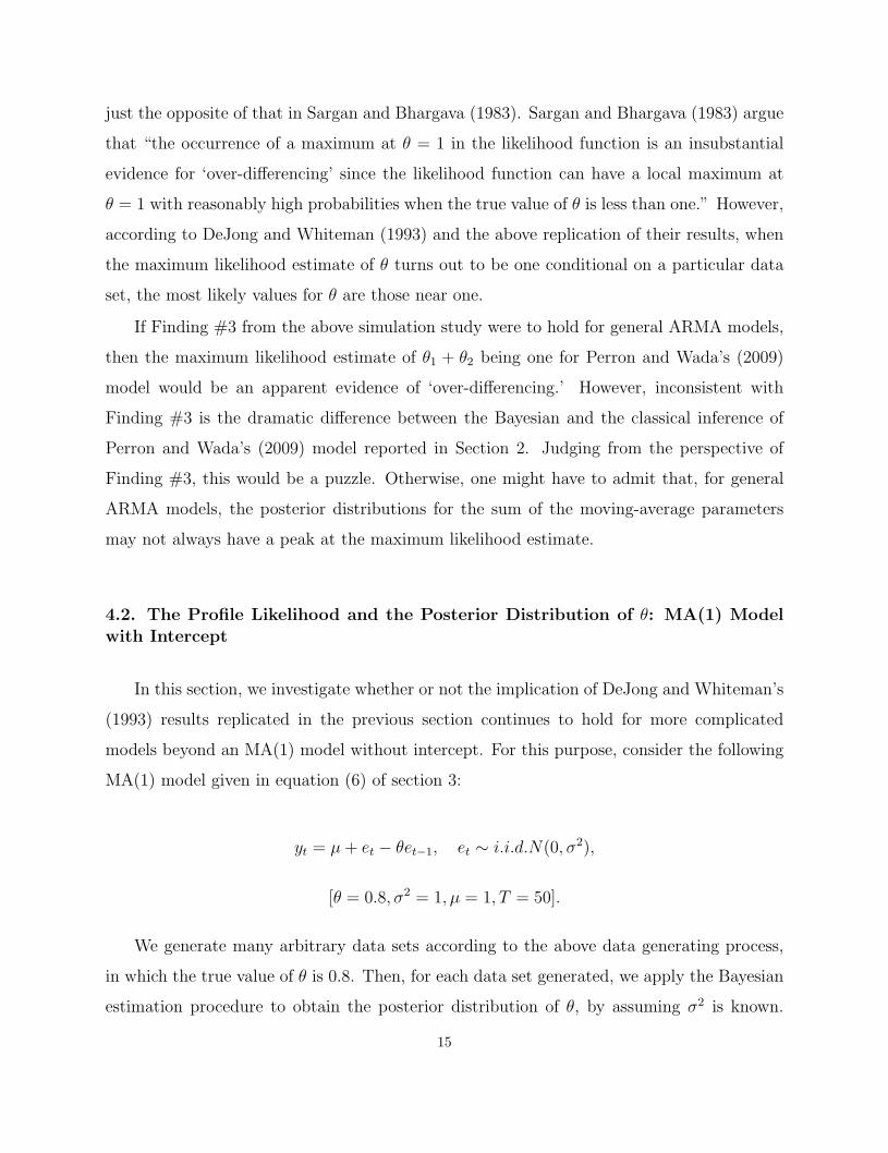
just the opposite of that in Sargan and Bhargava (1983). Sargan and Bhargava (1983) argue
that “the occurrence of a maximum at θ = 1 in the likelihood function is an insubstantial
evidence for ‘over-differencing’ since the likelihood function can have a local maximum at
θ = 1 with reasonably high probabilities when the true value of θ is less than one.” However,
according to DeJong and Whiteman (1993) and the above replication of their results, when
the maximum likelihood estimate of θ turns out to be one conditional on a particular data
set, the most likely values for θ are those near one.
If Finding #3 from the above simulation study were to hold for general ARMA models,
then the maximum likelihood estimate of θ1 + θ2 being one for Perron and Wada’s (2009)
model would be an apparent evidence of ‘over-differencing.’ However, inconsistent with
Finding #3 is the dramatic difference between the Bayesian and the classical inference of
Perron and Wada’s (2009) model reported in Section 2. Judging from the perspective of
Finding #3, this would be a puzzle. Otherwise, one might have to admit that, for general
ARMA models, the posterior distributions for the sum of the moving-average parameters
may not always have a peak at the maximum likelihood estimate.
4.2. The Profile Likelihood and the Posterior Distribution of θ: MA(1) Modelwith Intercept
In this section, we investigate whether or not the implication of DeJong and Whiteman’s
(1993) results replicated in the previous section continues to hold for more complicated
models beyond an MA(1) model without intercept. For this purpose, consider the following
MA(1) model given in equation (6) of section 3:
yt = µ + et − θet−1, et ∼ i.i.d.N(0, σ2),
[θ = 0.8, σ2 = 1, µ = 1, T = 50].
We generate many arbitrary data sets according to the above data generating process,
in which the true value of θ is 0.8. Then, for each data set generated, we apply the Bayesian
estimation procedure to obtain the posterior distribution of θ, by assuming σ2 is known.
15
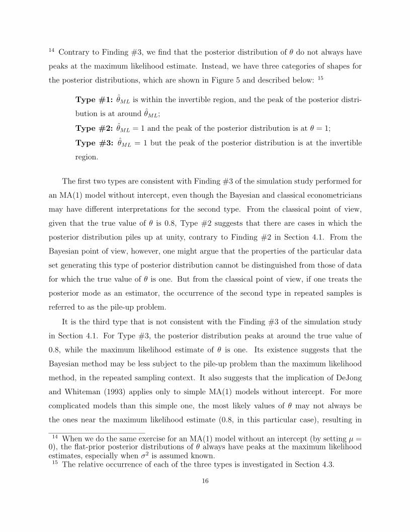
14 Contrary to Finding #3, we find that the posterior distribution of θ do not always have
peaks at the maximum likelihood estimate. Instead, we have three categories of shapes for
the posterior distributions, which are shown in Figure 5 and described below: 15
Type #1: θML is within the invertible region, and the peak of the posterior distri-
bution is at around θML;
Type #2: θML = 1 and the peak of the posterior distribution is at θ = 1;
Type #3: θML = 1 but the peak of the posterior distribution is at the invertible
region.
The first two types are consistent with Finding #3 of the simulation study performed for
an MA(1) model without intercept, even though the Bayesian and classical econometricians
may have different interpretations for the second type. From the classical point of view,
given that the true value of θ is 0.8, Type #2 suggests that there are cases in which the
posterior distribution piles up at unity, contrary to Finding #2 in Section 4.1. From the
Bayesian point of view, however, one might argue that the properties of the particular data
set generating this type of posterior distribution cannot be distinguished from those of data
for which the true value of θ is one. But from the classical point of view, if one treats the
posterior mode as an estimator, the occurrence of the second type in repeated samples is
referred to as the pile-up problem.
It is the third type that is not consistent with the Finding #3 of the simulation study
in Section 4.1. For Type #3, the posterior distribution peaks at around the true value of
0.8, while the maximum likelihood estimate of θ is one. Its existence suggests that the
Bayesian method may be less subject to the pile-up problem than the maximum likelihood
method, in the repeated sampling context. It also suggests that the implication of DeJong
and Whiteman (1993) applies only to simple MA(1) models without intercept. For more
complicated models than this simple one, the most likely values of θ may not always be
the ones near the maximum likelihood estimate (0.8, in this particular case), resulting in
14 When we do the same exercise for an MA(1) model without an intercept (by setting µ =0), the flat-prior posterior distributions of θ always have peaks at the maximum likelihoodestimates, especially when σ2 is assumed known.15 The relative occurrence of each of the three types is investigated in Section 4.3.
16

divergence between the inferences based on the Bayesian and the maximum likelihood meth-
ods. Furthermore, we think that the existence of the third type may explain the differences
between the Bayesian and classical inferences of Perron and Wada’s (2009) model reported
in Section 2. The existence of the third type definitely warrants more investigation and begs
an explanation.
As the model gets more complicated, we have more nuisance parameters. In this case,
a major difference between the two methods lies in the way these nuisance parameters are
handled. Following Smith and Naylor (1987) and Berger et al. (1999), we can explain
the reason for a potential divergence between the Bayesian and the classical inferences by
comparing the profile likelihood and the flat-prior posterior density (or integrated likelihood)
defined below:
Profile Likelihood : L(θ) = supµ L(θ, µ), (9)
Posterior Density (Integrated Likelihood) : L(θ) =∫
L(θ, µ)dµ, (10)
where L(θ, µ) is the likelihood function.
The posterior density of θ is not dependent upon the nuisance parameters, as it is ob-
tained by integrating the likelihood function with respect to the nuisance parameters. How-
ever, this is not always the case for the profile likelihood, as it is obtained by maximizing
with respect to the nuisance parameters. Pierce (1971) proves that, in a regression model
with ARMA(1,1) disturbances, the maximum likelihood estimator of θ and the regression co-
efficients (in our case, µ) are correlated in finite sample, even though they are asymptotically
independent and jointly normal. Thus, the likelihood function may not be quadratic, making
the shape of the profile likelihood different from that of the flat-prior posterior distribution
in small sample. This suggests that the posterior mode at the peak of the posterior density
may be different from the maximum likelihood estimate at the peak of the profile likelihood.
16
In order to illustrate how the profile likelihood and the posterior density can be different
in small sample (say, T = 50), we pick a representative sample from which each of the
16 But such finite sample discrepancy between the posterior mode and the maximum like-lihood estimate disappears as the sample size increases, because the maximum likelihoodestimators of µ and the nuisance parameters are asymptotically independent of each other.
17

above three types of the posterior distributions is obtained. For each data set, we draw a
three dimensional likelihood surface a 2-dimensional likelihood contour as a function of µ
and θ, by fixing σ2 at its true value. 17 The four angles of the three dimensional likelihood
function are drawn in Figure 6.A.1, 6.B.1, or 6.C.1. The likelihood contour is depicted in
Figure 6.A.2, 6.B.2, or 6.C.2, along with the corresponding profile likelihood and flat-prior
posterior distribution for θ. 18
For Type #1 and Type #2 in Figures 6.A.2 and 6.B.2, in which the posterior distributions
peak at θML, the shapes of the posterior density and the likelihood are very similar. Thus,
the Bayesian and the classical inferences may not be very different from each other. For
Type #3 in Figure 6.C.2, in which the posterior distribution does not peak at the maximum
likelihood estimate, the shapes of the profile likelihood and the posterior density are very
different from each other. Such a difference makes inferences based on the Bayesian and the
maximum likelihood method different. This is the case in which the correlation between θML
and µML is non-negligible in finite sample.
Note that, as shown in Type #3 of Figure 6.C.2, there may exist a local maximum in
the invertible region and it may be close to the posterior mode. From Tables 1.A and 1.B, in
which the classical and the Bayesian inferences are compared for Perron and Wada’s (2009)
ARMA model, the parameter values at the local maximum of the likelihood function are very
close to those at the posterior modes of the parameters. Besides, the posterior distribution
of θ1+θ2 does not peak at the maximum likelihood estimate of one. It peaks at the invertible
region. These suggest that the results reported in Tables 1.A and 1.B for Perron and Wada’s
(2009) model may be an example of Type #3.
4.3. Sampling Distributions for the Posterior Mode of θ: Monte Carlo Experi-ment
For Bayesians, there is only one realization of the data set, so contemplating the proba-
17 This does not affect the results, as the maximum likelihood estimator for σ2 is indepen-dent of that for the rest of the parameters in the model.18 The three posterior distributions shown in Figure 5 are the same as those in Figures
6.A.2, 6.B.2, and 6.C.2 in order.
18

bility of the pile-up problem in repeated sampling may be conceptually irrelevant. However,
in order for us to be able to evaluate and directly compare the probabilities of the pile-up
problem for both the Bayesian and classical approaches, we have no choice but to treat
the posterior mode of θ as a Bayesian estimator, which is treated as a random variable in
repeated samples.
In this section, we evaluate the relative frequencies of Type #2 occurring in repeated
samples, or the probabilities of the pile-up effect for the Bayesian approach, for various
models and sample sizes. These are compared to the relative frequencies of Type #2 or
Type #3 occurring, or the probabilities of the pile-up effect for the maximum likelihood
approach, which are invested in Section 3. For this purpose, we perform a Monte Carlo
experiment, by generating 5,000 sets of data according to each data generating process in
equations (5)-(8) of Section 3. For each of the models and sample sizes (T = 50, 100,
200), we get the sampling distribution for the posterior mode of θ. 19 Throughout the
MCMC iterations, we impose the constraint that |θ| < 1. Thus, as in Section 3, we report
Pr[0.995 < θmode < 1] as the probability of the pile-up problem, where θmode is the posterior
mode of θ.
The results are depicted in Figure 7 and summarized in Table 3, along with the proba-
bilities of the pile-up problem. As in the case of the maximum likelihood approach reported
in Table 2, the probabilities of the pile-up problem increase as the model gets more compli-
cated; they decrease as the sample size increases. Without an exception, however, for all the
models and sample sizes considered, the probabilities of the pile-up problem are ‘consider-
ably’ smaller than in the case of the maximum likelihood approach. For example, when the
sample size as big as 200, the Bayesian approach does not suffer from the pile-up problem,
even for an ARMA(1,1) model with a structural break in intercept, the most complicated
model under consideration. Note that, under the same situation, the probability of the
pile-up problem remain as high as 0.24 for the maximum likelihood approach.
Based on the results in this section, along with those in Section 3, we can conclude that
the Bayesian approach suffers considerably less from the pile-up problem than the maximum
19 The model is estimated based on the MCMC algorithm proposed by Chib and Greenberg(1994). For a brief description of the algorithm, readers are referred to Appendix B. Thepriors we employ for (µ, µ1, φ, θ) are N(0, 102), and the prior for σ2 is diffuse.
19

likelihood approach. This allows us to confer more credibility to the Bayesian inference of
Perron and Wada’s (2009) model reported in Table 1.B, Figures 1.A and 1.B.
5. Empirical Results: Let’s Take Uncertain Breaks
In this section, we relax the assumption of a known break date for the mean growth
rate in Perron and Wada’s (2009) ARMA(2,2) model of real GDP growth. We believe
that incorporating uncertainty in the break date is equally as important as incorporating
uncertainty in the rest of the parameters of the model. A reduction in the variance of the
shocks to real GDP, namely the Great Moderation (Kim and Nelson (1999) and McConnell
and Perez-Quiros (2000)), is also incorporated. The model we estimate using the Bayesian
approach is given by:
∆yt = µ0 + µ1St + ∆y∗
t ,
∆y∗
t = φ1∆y∗
t−1 + φ2∆y∗
t−2 + et − θ2et−1 − θ2et−2, (11)
et|Dt ∼ i.i.dN(0, (1 − Dt)σ20 + Dtσ
21),
P r[St = 0|St−1 = 0] = p00, P r[St = 1|St−1 = 1] = 1,
P r[Dt = 0|Dt−1 = 0] = q00, P r[Dt = 1|Dt−1 = 1] = 1,
where ∆yt is the real GDP growth rate, ∆y∗
t is the demeaned growth rate. We incorporate
uncertainty in the break dates for mean and variance by restricting the transition proba-
bilities of St and Dt to allow for an absorbing state. 20 The estimates of the expected
durations of regime 0 (i.e., 1/(1− p00) and 1/(1− pq00)) are the estimates of the break dates.
For Bayesian estimation of the above model, we employ a multi-move Markov-Chain Monte
Carlo (MCMC) algorithm recently proposed by Kim and Kim (2013). 21
Figure 8.A depicts the cumulative posterior probabilities of a structural break in the
mean and the variance of real GDP growth. The nature of the structural break in the
20 This approach has been suggested by Chib (1998).21 For a brief description of the algorithm, readers are referred to Appendix B.
20

variance is such that the structural break is very sharp, leaving little uncertainty in the
break date. However, it is interesting to observe that the structural break in the mean
growth rate is not very sharp, leaving considerably high uncertainty in the break date.
Table 4 reports the posterior moments of the model parameters, along with their 90
percent HPD (highest posterior density) interval. The posterior mean and mode of θ1 + θ2
are 0.137 and 0.427, respectively, with the 90 percent HPD interval is [−0.554, 0.873]. Note
that, unlike in the Bayesian inference of Perron and Wada’s (2009) model reported in Table
1.B, the 90% HPD interval does not cover the non-invertible boundary of one. The posterior
distribution of θ1 + θ2 shown in Figure 8.A also confirms this. It is unimodal and it has little
probability mass at unity. The impulse-response analysis in Figure 8.B shows that a shock
to real output generates highly persistent fluctuations in real GDP. With the incorporation
of Great Moderation and uncertainty in the break dates, the posterior mode for the long-run
impulse-response coefficient (1.575) reported in Table 4 is even larger than that (1.359) for
the Perron and Wada model reported in Table 1.B, with the 90 percent HPD interval being
[1.189, 2.034]. All these results imply that it is highly unlikely that the log of real GDP
may be a trend stationary process, contrary to the implication of the classical inference for
Perron and Wada’s (2009) model.
Figure 8.B depicts the posterior modes of the trend and the cyclical components of real
GDP. The trend component explains most of the variations in real output and the resulting
cyclical component is small in magnitude and noisy. That is, even after taking breaks
with uncertain break dates, the implications of Nelson and Plosser (1982) and Morley et al.
(2003) on trend-cycle decomposition continue to hold within the Bayesian framework, which
is relatively free from the pile-up problem.
6. Summary and Conclusion
A conventional belief is that a non-informative prior leads to the Bayesian posterior
mode being very close to the maximum likelihood estimate, since the maximum likelihood
estimate is not influenced by priors. If this is the case, the most likely values for the param-
eter of interest would be those near the maximum likelihood estimate, from the Bayesian
21

perspective. We show that this common belief does not apply to general ARMA models,
especially when there is a structural break in mean. There are cases in which we may have
the posterior mode of the moving-average parameter inside the invertible region, even when
the maximum of the likelihood function occurs at unity. In the repeated sampling context,
this suggests that the Bayesian approach may suffer much less from the pile-up problem than
the maximum likelihood approach, which is confirmed by our simulation study.
Based on maximum likelihood estimation of an ARMA model of real GDP growth with
a structural break in mean, Perron and Wada (2009) show that real GDP may be a trend
stationary process. On the contrary, our results based on Bayesian estimation of the same
model implies that most of the variations in real GDP can be explained by the stochastic
trend component, consistent with the implications of Nelson and Plosser (1982) and Morley
et al. (2003).
Our analysis indicates that Perron and Wada’s (2009) results may be due to the pile-up
problem, to which the maximum likelihood method is subject in finite sample. Based on a
Monte Carlo experiment, which is performed by taking the posterior modes of the parameters
for Perron and Wada’s (2009) model as true values, we show that the probability of the pile-
up problem for the maximum likelihood approach is as high as 0.4. We conclude that, even
after taking a break in the mean growth rate of real GDP in the mid 1970s, the implications of
Nelson and Plosser (1982) and Morley et al. (2003) on trend-cycle decomposition continue to
hold within the Bayesian framework, which is relatively free from the pile-up problem. This
conclusion is further strengthened if we incorporate the Great Moderation, i.e., a structural
break in the conditional variance of real GDP in the mid-1980s, and uncertainty in the break
dates.
22
Appendix A. Generating ARMA Parameters
A slightly modified version of the recursive data transformation schemes by Chib and
Greenberg (1994) is introduced in this section, which produces simple Gaussian linear regres-
sion relationships for ARMA parameters. For illustrative purposes, consider the following
ARMA(1,1) model with a mean:
yt = µ + φ(yt−1 − µ) + et − θet−1, et ∼ i.i.d.N(0, σ2). (A.1)
We employ Metropolis-Hastings algorithm at each of the following candidate generating
processes. The candidate at each step is generated with (y0 − µ) = e0 = 0 and is then tried
in an Metropolis-Hastings step to take into account the uncertainty associated with the initial
values. The candidate is accepted or rejected according to an acceptance probability which
can be easily calculated by casting the above ARMA model into a state-space representation
and using the conventional Kalman filter.
A.1. Data Transformation for φ conditional on data (YT ), and other parameters
The following is the necessary data transformation step for generating φ:
Y = Xφ + e, (A.2)
yt = yt − µ − θ yt−1, xt = yt−1,
where Y = [y1 y2 ... yT ]′; X = [x1 x2 ... xT ]′; e = [e1, e2, ..., eT ]′; yt = 0 for t < 0, y0 =
e0 = 0. The above derivation of data transformation can be easily shown by the fact that
et = yt − xtφ. The mean and the variance of the posterior candidate density is defined by
φ = Φ(Φ−1φ + σ−2X ′Y ) and Φ(Φ−1 + σ−2X ′X)−1 where φ and Φ are a prior mean and a
prior variance, respectively.
A.2. Data Transformation for µ conditional on YT and other parameters
23

We show recursive data transformations for generating µ:
Y ∗ = X∗µ + e, (A.3)
y∗
t = yt − φ yt−1 − θ y∗
t−1,
x∗
t = (1 − φ) − θ x∗
t−1,
where Y ∗ = [y∗
1 y∗
2 ... y∗
T ]′; X∗ = [x′∗
1 x′∗
2 ... x′∗
T ]′; e = [e1, e2, ..., eT ]′; yt = y∗
t = 0 for t < 0
and y0 = y∗
0 = e0 = 0; the vectors xt = x∗
t = 0 for t ≤ 0. The above derivation of
data transformation can be easily shown by the fact that et = y∗
t − x∗
t µ. We generate a
candidate µ based on the conventional normal posterior candidate generating density. The
mean and the posterior covariance matrix are defined by µ = Ωµ(Ωµ−1µ + σ−2X∗′Y ∗) and
Ωµ = (Ω−1µ +σ−2X∗′X∗)−1 where µ and Ωµ are a prior mean and a prior variance, respectively.
A.3. Data Transformation for θ conditional on YT and other parameters
In order to generate θ, Chib and Greenberg (1994) suggested a candidate density of θ
based on the first-order Taylor expansion and the non-linear least-squares estimation. By
the first-order Taylor expansion, et(θ) ≈ et(θ∗) + ωt(θ − θ∗) = (et(θ
∗) − ωtθ∗) + ωtθ where
θ∗ denotes the nonlinear least squares estimate of θ and ωt = ∂et(θ)∂θ
|θ=θ∗ . The recursive data
transformation is given by:
Y ≈ Xθ + e, (A.4)
yt = et(θ∗) − ωtθ
∗,
xt = −ωt,
where Y = [y1 y2 ... yT ]′; X = [x1 x2 ... xT ]′; e = [e1, e2, ..., eT ]′; yt = yt = 0 for t <
0 and y0 = e0 = 0; the vectors xt = 0 for t ≤ 0. The above approximation provides
a convenient way to generate a candidate θ based on the conventional normal posterior
candidate generating density. The mean and the posterior covariance matrix are defined by
θ = Ωθ(Ωθ−1θ + σ−2X ′Y ) and Ωθ = (Ω−1
θ + σ−2X ′X)−1 where θ and Ωθ are a prior mean
and a prior variance, respectively.
24

A.4. Data Transformation for σ2 conditional on Y and all the other parameters
The posterior simulation on σ2 is straightforward given one of the previously transformed
data sets. The posterior samples on σ2 are drawn from the following conditional posterior
density:
Prior : σ2 ∼ IG(ν
2,δ
2), (A.5)
Posterior : σ2|YT , ST , Ψ−σ2 ∼ IG(ν
2,δ
2),
where ν and δ are a prior degree of freedom and a prior scale parameter, respectively;
ν = ν + T ; δ = δ + d where d =∏T
t=0 e2t =
∏Tt=0(yt − xtφ)2. Note that alternatively, other
transformed data set (Y ∗, X∗) can be used to calculate d.
Appendix B. Multi-move Algorithm By Kim and Kim (2013)
In this appendix, we explain how to implement the efficient muti-move sampler for
latent regime indicator variable St based on Metropolis-Hastings algorithm. For notational
simplicity, we suppress the other model parameters in the conditional densities that follows.
First, consider the following decomposition of the target density F (ST |YT ):
F (ST |YT ) = f(ST |YT )T−1∏
t=0
f(St|St+1:T , YT ), (B.1)
where ST = [S0, S1, ..., ST ]′; Y = [Y1, Y2, ..., YT ]′; St+1:T = [ St+1 St+2 . . . ST ]′.
The above decomposition suggests that one can sequentially generate ST from f(ST |YT ),
and then St from the conditional density f(St|St+1:T , YT ), for t = T −1, ..., 0. The individual
conditional densities can be further decomposed as follows:
25

f(St|St+1:T , YT ) = f(St|St+1:T , Yt, Yt+1:T )
=f(St, Yt+1:T |St+1:T , Yt)
f(Yt+1:T |St+1:T , Yt)
∝ f(St, Yt+1:T |St+1:T , Yt)
= f(St|St+1:T , Yt) f(Yt+1:T |St:T , Yt)
∝ f(St+1|St)f(St|Yt)T∏
k=t+1
f(yk|St:k, Yk−1),
(B.2)
where Yt = [ y1 y2 . . . yt ]′; Yt+1:T = [ yt+1 yt+2 . . . yT ]′. Even if one can use (B.1)
and (B.2) to generate ST theoretically, evaluating (B.2) is not feasible in practice due to
a non-trivial moving-average structure. Thus, Metropolis-Hastings algorithm is used to
overcome the difficulty.
Kim and Kim (2013) propose to sequentially generate St, t = T, T − 1, ..., 1, 0, from
the individual proposal density given below, as an approximation to the density in equation
(B.2):
g(St|St+1:T , YT ) ∝ f(St+1|St)h(St|Yt), (B.3)
where f(St+1|St) is the transition probability and the h(St|Yt) term is an approximation
to the f(St|Yt) term in equation (B.2). Kim and Kim (2013) employ the approximate
algorithm by Kim (1994) to obtain h(St|Yt). For details of Kim’s (1994) approximate Kalman
filter to calculate h(St|Yt), readers are referred to Kim (1994) and Kim and Kim (2013).
An additional approximation involved is that∏T
k=t+1 f(yk|St:k, Yk−1) from equation (B.2) is
ignored.
Once ST is generated from the multi-move candidate density in equation (B.3), the whole
sequence of S0, S1, ..., ST is globally accepted or rejected, using an appropriate acceptance
probability. Let SJT and SJ−1
T be the sequences of S0, S1, ..., ST generated at the current
and the previous iterations of the MCMC algorithm, respectively. Then, the acceptance
probability is given by:
α(SJT , SJ−1
T ) = min
[
F (SJT |YT )
F (SJ−1T |YT )
G(SJ−1T |YT )
G(SJT |YT )
, 1
]
, (B.4)
26

where F (.|YT ) is given in equation (B.1), as rewritten below:.
F (ST |YT ) =f(ST ) f(YT |ST )
f(YT )
=f(S0)
∏Tt=1 f(St|St−1)
∏Tt=1 f(yt|St, Yt−1)
f(YT ),
(B.5)
and G(.|YT ) is the multi-move candidate density defined below:
G(ST |YT ) =T∏
t=0
[
g(St|St+1:T , YT )∑
Stg(St|St+1:T , YT )
]
=T∏
t=0
[
f(St+1|St)h(St|Yt)∑
Stf(St+1|St)h(St|Yt)
]
=T∏
t=0
[
f(St+1|St)h(St|Yt)
h(St+1|Yt)
]
. (B.6)
By substituting equations (B.5) and (B.6) into equation (B.4), we can derive the following
acceptance probability:
α(SJT , SJ−1
T ) = min
[
T∏
t=1
f(yt|SJt , Yt−1)
f(yt|SJ−1t , Yt−1)
T∏
t=1
h(SJ−1t |Yt)
h(SJt |Yt)
T−1∏
t=0
h(SJt+1|Yt)
h(SJ−1t+1 |Yt)
, 1
]
, (B.4′)
where h(St|Yt) can be obtained by applying the approximate filter of Kim (1994) and
f(yt|St, Yt−1) can be evaluated by applying the conventional Kalman filter to the state-space
model.
27

References
[1] Anderson, T.W. and A., Takemura, 1986, “Why do noninvertible estimated moving
averages occur?” Journal of Time Series Analysis 7, 235-54.
[2] Ansley, Craig F., and Paul Newbold, 1980, “Finite Sample Properties of Estimators for
Autoregressive Moving Average Models,” Journal of Econometrics XIII, 1959-83.
[3] Berger, J.O, B. Liseo, and R.L. Wolpert, 1999, “Integrated Likelihood Methods for
Eliminating Nuisance Parameters,” Statistical Science 1999, Vol. 14, No. 1, 1-28.
[4] Beveridge, S., and C. R. Nelson, 1981, “A New Approach to Decomposition of Economic
Time Series into Permanent and Transitory Components with Particular Attention to
Measurement of the ’Business Cycle’,” Journal of Monetary Economics 7, 151-174.
[5] Campbell, John Y. and Gregory N. Mankiw, 1987, “Are output fluctuations transitory?,”
Quarterly Journal of Economics 102, 857-880.
[6] Cheung, Y.N., Chinn, M., 1997, “Further Investigation of the Uncertain Unit Root in
U.S. GDP,” Journal of Business and Economic Statistics 15, 68-73.
[7] Chib, S., 1998, “Estimation and comparison of multiple change-point models,” Journal
of Econometrics, 86, 221-241.
[8] Chib, S., and Edward Greenberg, 1994, “Bayes Inference in Regression Models with
ARMA(p,q) Errors,” Journal of Econometrics 64, 183-206.
[9] Christiano, L.J., 1992, “Searching for breaks in GNP,” Journal of Business and Economic
Statistics 10, 237-250.
[10] Clark, P. K., 1987, “The Cyclical Component of U.S. Economic Activity,” Quarterly
Journal of Economics 102, 798-814.
[11] Davis R. A., Chen MC, and Dunsmuir, W.T.M., 1995, “Inference for MA(1) Processes
with a Root on or near the Unit Circle,” Probability and Mathematical Statistics 15,
227-242.
[12] Davidson, J.E.H., 1981, “Problems with the Estimation of Moving Average Processes,”
Journal of Econometrics 16, 295-310.
[13] DeJong, David N., John C. Nankervis, N. E. Savin and Charles H. Whiteman, 1992,
“Integration Versus Trend Stationary in Time Series,” Econometrica, Vol. 60, No. 2,
28

423-433.
[14] DeJong and Whiteman, 1991, “Reconsidering Trends and random walks in macroeco-
nomic time series” Journal of Monetary Economics 28, 221-254.
[15] DeJong, D. N. and C. H. Whiteman, 1993, “Estimating Moving Average Parameters:
Classical Pile-ups and Bayesian Posteriors,” Journal of Business and Economic Statistics
64, 183-206.
[16] Diebold, Francis X., and Abdelhak S. Senhadji, 1996 “The Uncertain Unit Root in Real
GNP: Comment,” American Economic Review 86, 1291-98.
[17] Gospodinov, N., 2002, “Bootstrap-Based Inferences in Models With a Nearly Noninvert-
ible Moving Average Component,” Journal of Business & Economic Statistics, Vol. 20,
No. 2, 254-268.
[18] Harvey, A. C., 1985, “Trends and Cycles in Macroeconomic Time Series,” Journal of
Business and Economic Statistics 3, 216-227.
[19] Kang, K. M., 1975, “A Comparison of Estimators for Moving Average Processes,” Un-
published Paper, Australian Bureau of Statistics.
[20] Kim, Chang-Jin, and Nelson, C. R., 1999, “Has the U.S. Economy Become more Stable?
A Bayesian Approach based on a Markov-Switching Model of the Business Cycle,” The
Review of Economics and Statistics 81,608-616.
[21] Kim, Chang-Jin and Jaeho Kim, 2013, “Bayesian Inference of Regime-Switching ARMA
Models with Absorbing States: Dynamics of Ex-Ante Real Interest Rate Under Struc-
tural Breaks,” Working Paper, University of Washington.
[22] McConnell, M. and Perez Quiros, G., 2000, “Output Fluctuations in the United States:
What has Changed Since the Early 1980s?” American Economic Review 90, 1464-1476.
[23] Morley, James C., Charles R. Nelson, Eric Zivot, 2003, “Why are the Beveridge-Nelson
and Unobserved-Components Decompositions of GDP so Different?” The Review of
Economics and Statistics 85, 235-243.
[24] Murray, C. J. and C. R. Nelson, 2000, “The Uncertain Trend in U.S. GDP,” Journal of
Monetary Economics 46, 79-95.
[25] Murray, C., and C. R. Nelson, 2002, “The Great Depression and Output Persistence,”
Journal of Money, Credit and Banking 34, 1090-1098.
29

[26] Nelson, C. R., and Plosser, C. I., 1982, “Trends and Random Walks in Macroeconomic
Time Series: Some Evidence and Implications,” Journal of Monetary Economics 10,
139-162.
[27] Newbold, Paul, Stephen Leybourne, and Mark E. Wohar, 2001, “Trend Stationarity,
Difference Stationarity, or Neither: Further Diagnostic Tests with an Application to
U.S. Real GNP, 1875-1993,” Journal of Economics and Business 53, 85-102.
[28] Perron, P., 1989, “The great crash, the oil price shock, and the unit root hypothesis,”
Econometrica 57, 1361-1401.
[29] Perron, P., Wada, T., 2009, Let’s Take a Break: Trends and Cycles in US Real GDP,
Journal of Monetary Economics 56(6), 749-765.
[30] Pierce, D., 1971, “Least Squares Estimation in the Regression Model with Autoregressive
Moving Average Errors,” Biometrika, Vol. 58, No. 2, 299-312
[31] Plosser, C. I., and G. W. Schwert, 1977, “Estimation of a Non-Invertible Moving Average
Process: The Case of Over-differencing,” Journal of Econometrics, 6, 199-224.
[32] Sargan, JD, Bhargava, A., 1983, “Maximum Likelihood Estimation of Regression Mod-
els with First-Order Moving Average Errors when the Root Lies on the Unit Circle,”
Econometrica 51, 799-820.
[33] Shephard, N. G., and A. C. Harvey, 1990, “On the Probability of Estimating a Deter-
ministic Component in the Local Level Model,” Journal of Time Series Analysis, 11,
339-347.
[34] Shephard, Neil, 1993, “Maximum Likelihood Estimation of Regression Models with
Stochastic Trend Components,” Journal of American Statistical Association 88, 590-
595.
[35] Sims, C. A., and Uhlig, H., 1991, “Understanding Unit Rooters: A Helicopter Tour,”
Econometrica Vol. 5, No. 9, 1591-1600.
[36] Smith, Richard and J.C. Naylor, 1987, “A Comparison of Maximum Likelihood and
Bayesian Estimators for the Three-Parameter Weibull Distribution,” Journal of the Royal
Statistical Society Series C (Applied Statistics) 36, No. 3, 358-369.
[37] Stock, J. H., 1994, “Unit Roots, Structural Breaks, and Trends,” Chapter 46 of Handbook
of Econometrics, Volume IV, Edited by R.F. Engle and D.L. McFadden, Elsevier Science.
30

[38] Stock, J. H., and Watson, M. W., 1998, “Median Unbiased Estimation of Coefficient
Variance in a Time-Varying Parameter Model,” Journal of the American Statistical As-
sociation 93, 349-358.
[39] Tanaka, K. and S. E. Satchell, 1989, “Asymptotic Properties of the Maximum Likelihood
and Non-linear Least Squares Estimator for Noninvertible Moving Average Models,”
Econometric Theory 5, 333-353.
[40] Zivot, E., and Andrews, D.W.K., 1992, “Further Evidence on the Great Crash, the Oil-
Price Shock and the Unit Root Hypothesis,” Journal of Business and Economic Statistics
10, 251-287.
31

Table 1.A. Maximum Likelihood Estimates[ Perron and Wada’s (2009) Model (1947:1~1998:2) ]
∆ ∆ , ∆ ∆ ∆ , ~ . . 0, σ , 0 1973: 1, 1 1973: 1.
Parameters
Global Maximum
Local Maximum
Estimates
S.E.
Estimates
S.E.
0.951 0.021 0.979 0.116
-0.287 0.038 -0.332 0.166
0.921 0.020 0.630 0.104
-0.601 0.109 -0.731 0.150
0.999 0.003 0.546 0.142
-0.283 0.137 -0.542 0.211 σ 0.876 0.086 0.922 0.091
Long-run
Impulse-Response
0.000
0.042
1.228
0.312
Log Likelihood
-278.930
-282.710
Note: 1. Quarterly real GDP (Seasonally adjusted) from 1947:1 to 1998:2 are used for producing results.
2. S.E. refers to the standard errors of the estimates.
3. S.E. of the long-run impulse response is reported using delta method.
4. Actual estimate of is 0.9999.

Table 1.B. Bayesian Estimates[ Perron and Wada’s (2009) Model (1947:1~1998:2) ]
∆ ∆ , ∆ ∆ ∆ , ~ . . 0, σ , 0 1973: 1, 1 1973: 1.
Parameters
Prior
Posterior
Mean
SD
Mean
Mode
SD
90 % HPDI
1.2 2 0.996 0.952 0.129 [0.780, 1.218]
-0.5 2 -0.363 -0.309 0.176 [-0.650, -0.056]
0.5 2 0.500 0.620 0.265 [0.079, 0.941]
-0.5 2 -0.426 -0.571 0.267 [-0.840, 0.062]
0.5 2 0.286 0.498 0.413 [-0.345, 1.000]
-0.5 2 -0.337 -0.340 0.189 [-0.663, 0.006] σ 1 2 0.959 0.937 0.097 [0.799, 1.120]
Long-run
Impulse-Response
1.359
1.387
0.318
[0.951,1.869]
Note: 1. Quarterly real GDP (Seasonally adjusted) from 1947:1 to 1998:2 are used for producing results.
2. Burn-in / Total iterations =5,000 / 105,000
3. S.D. refers to the standard deviations of the posterior distributions.
4. A highest posterior density interval (HPDI) is an interval, the narrowest one possible with a chosen
probability.
5. Bayesian algorithm by Chib and Greenberg (1993) is used for estimation.
6. The acceptance probabilities of the Metropolis-Hastings algorithm in MCMC are all above 0.85.

Table 2. Sampling Distributions of Maximum Likelihood estimators for θ and the Probabilities of
the Pile-up Problem: Monte Carlo Experiment
, , ~ . . 0, 0, ; 1, , 1,2, . . ,
[ 0.8; 1; 1; 0.3, 0.3 ]
Pr 0.8
Prob. of Pile-up
0.6
0.7
0.8
0.9
1
MA(1) without Intercept
0.025 0.124 0.425 0.755 1 0.119 0.001 0.051 0.442 0.906 1 0.016 0.000 0.011 0.471 0.979 1 0.000
MA(1) with Intercept
0.016 0.070 0.238 0.403 1 0.582 0.001 0.038 0.329 0.752 1 0.169 0.000 0.008 0.374 0.948 1 0.008
MA(1) with a Structural Break in Intercept
0.008 0.037 0.104 0.133 1 0.867 0.002 0.028 0.215 0.520 1 0.447 0.000 0.007 0.301 0.891 1 0.044
ARMA(1,1) with a Structural Break in Intercept
0.027 0.042 0.058 0.060 1 0.939 0.025 0.067 0.165 0.263 1 0.730 0.010 0.058 0.281 0.665 1 0.236
Note:
We report Pr 0.995 1 as the probability of the pile-up problem, as in DeJong and Whiteman
(1993).

Table 3. Sampling Distributions of Bayesian Posterior Modes for θ and the Probabilities of the
Pile-up Problem: Monte Carlo Experiment
, , ~ . . 0, 0, ; 1, , 1,2, . . ,
[ 0.8; 1; 1; 0.3, 0.3 ]
Pr 0.8
Prob. of Pile-up
0.6
0.7
0.8
0.9
1
MA(1) without Intercept
0.035 0.143 0.446 0.777 1 0.083 0.002 0.062 0.453 0.902 1 0.010 0.000 0.013 0.467 0.975 1 0.000
MA(1) with Intercept
0.044 0.157 0.407 0.631 1 0.110 0.004 0.072 0.455 0.860 1 0.013 0.000 0.016 0.462 0.973 1 0.003
MA(1) with a Structural Break in Intercept
0.055 0.172 0.365 0.533 1 0.197 0.007 0.080 0.435 0.808 1 0.037 0.000 0.018 0.456 0.957 1 0.003
ARMA(1,1) with a Structural Break in Intercept
0.183 0.257 0.341 0.441 1 0.241 0.102 0.239 0.422 0.653 1 0.137 0.030 0.129 0.458 0.855 1 0.006
Note: We report Pr 0.995 1 as the probability of the pile-up problem, as in DeJong and
Whiteman (1993)., where is the posterior mode of θ.

Table 4. Bayesian Estimates [ARIMA Model with Unknown Break Points in the Mean and
the Variance (1947:1~1998:2) ]
∆ ∆ , ∆ ∆ ∆ , | ~ . . 0, 1 σ σ , Pr 0| 0 , Pr 1| 1 1, Pr 0| 0 , Pr 1| 1 1.
Parameters
Prior
Posterior
Mean
SD
Mean
Mode
SD
90 % HPDI
0.99 0.01 0.988 0.993 0.009 [0.975, 0.999]
0.99 0.01 0.991 0.995 0.005 [0.983, 0.999]
1.2 2 1.048 0.928 0.233 [0.703, 1.456]
-0.5 2 -0.349 -0.231 0.232 [-0.678, 0.000]
0.5 2 0.456 0.600 0.254 [0.029, 0.925]
-0.5 2 -0.298 -0.464 0.305 [-0.775, 0.226]
0.5 2 0.137 0.427 0.402 [-0.554, 0.873]
-0.5 2 -0.302 -0.334 0.191 [-0.608, 0.062] σ 1 2 1.277 1.219 0.153 [1.024, 1.556] σ 1 2 0.245 0.225 0.048 [0.166, 0.331]
Long-run Impulse-
Response
1.575
1.519
0.298
[1.189, 2.034]
Note: 1. Quarterly real GDP (Seasonally adjusted) from 1947:1 to 1998:2 are used for producing results.
2. Burn-in / Total iterations =5,000 / 105,000
3. S.D. refers to the standard deviations of the posterior distributions.
4. A highest posterior density interval (HPDI) is an interval, the narrowest one possible with a chosen
probability.
5. Bayesian algorithms by Kim and Kim (2013), Chib and Greenberg (1993) are used for estimation.
6. The acceptance probabilities of the Metropolis-Hastings algorithms in MCMC are all above 0.85.

Figure 1.A. Posterior Distributions for the Sum of MA Parameters and Long-Run Impulse-
Response Coefficient [ Perron and Wada’s (2009) Model (1947:1~1998:2) ]
( ) .
Long-run Impulse Response Coefficient
Note: 1. The model is estimated by the MCMC algorithm by Chib and Greenberg (1993). The total number
of Bayesian MCMC iteration is 105,000 and the first 5,000 samples are discarded.
.000
.004
.008
.012
.016
.020
.024
.028
-1.0 -0.8 -0.6 -0.4 -0.2 0.0 0.2 0.4 0.6 0.8 1.0
Re
lati
ve
Fre
qu
en
cy
.00
.01
.02
.03
.04
.05
.06
0.00 0.25 0.50 0.75 1.00 1.25 1.50 1.75 2.00 2.25 2.50 2.75 3.00
Re
lati
ve
Fre
qu
en
cy

Figure 1.B. Comparison of Classical and Bayesian Inferences: Trend-Cycle Decomposition and
Impulse-Response Analysis [ Perron and Wada’s (2009) Model (1947:1~1998:2) ] ( ) .
Classical Inference
Bayesian Inference
Log of Real GDP vs. Trend Component
Cyclical Component
Impulse-Response Analysis
Note: 1. The model is estimated by the MCMC algorithm by Chib and Greenberg (1993). The total number
of Bayesian MCMC iteration is 105,000 and the first 5,000 samples are discarded.
2. The confidence band for the impulse-response function analysis is calculated by the Delta method.
720
760
800
840
880
920
1950 1955 1960 1965 1970 1975 1980 1985 1990 1995
Trend GDP
720
760
800
840
880
920
1950 1955 1960 1965 1970 1975 1980 1985 1990 1995
Trend GDP
-8
-6
-4
-2
0
2
4
6
1950 1955 1960 1965 1970 1975 1980 1985 1990 1995
-8
-6
-4
-2
0
2
4
6
1950 1955 1960 1965 1970 1975 1980 1985 1990 1995
-0.4
0.0
0.4
0.8
1.2
1.6
2.0
3 6 9 12 15 18 21 24 27 30
0.0
0.4
0.8
1.2
1.6
2.0
3 6 9 12 15 18 21 24 27 30

Figure 2. Sampling Distributions of Maximum Likelihood estimators for θ: Monte Carlo Experiment
Model #1 (T=50) Model #1 (T=100) Model #1 (T=200)
Model #2 (T=50) Model #2 (T=100) Model #2 (T=200)
Model #3 (T=50) Model #3 (T=100) Model #3 (T=200)
Model #4 (T=50) Model #4 (T=100) Model #4 (T=200)
0.0
0.2
0.4
0.6
0.8
1.0
0.0 0.1 0.2 0.3 0.4 0.5 0.6 0.7 0.8 0.9 1.0
0.0
0.2
0.4
0.6
0.8
1.0
0.0 0.1 0.2 0.3 0.4 0.5 0.6 0.7 0.8 0.9 1.0
0.0
0.2
0.4
0.6
0.8
1.0
0.0 0.1 0.2 0.3 0.4 0.5 0.6 0.7 0.8 0.9 1.0
0.0
0.2
0.4
0.6
0.8
1.0
0.0 0.1 0.2 0.3 0.4 0.5 0.6 0.7 0.8 0.9 1.0
0.0
0.2
0.4
0.6
0.8
1.0
0.0 0.1 0.2 0.3 0.4 0.5 0.6 0.7 0.8 0.9 1.0
0.0
0.2
0.4
0.6
0.8
1.0
0.0 0.1 0.2 0.3 0.4 0.5 0.6 0.7 0.8 0.9 1.0
0.0
0.2
0.4
0.6
0.8
1.0
0.0 0.1 0.2 0.3 0.4 0.5 0.6 0.7 0.8 0.9 1.0
0.0
0.2
0.4
0.6
0.8
1.0
0.0 0.1 0.2 0.3 0.4 0.5 0.6 0.7 0.8 0.9 1.0
0.0
0.2
0.4
0.6
0.8
1.0
0.0 0.1 0.2 0.3 0.4 0.5 0.6 0.7 0.8 0.9 1.0
0.0
0.2
0.4
0.6
0.8
1.0
0.0 0.1 0.2 0.3 0.4 0.5 0.6 0.7 0.8 0.9 1.0
0.0
0.2
0.4
0.6
0.8
1.0
0.0 0.1 0.2 0.3 0.4 0.5 0.6 0.7 0.8 0.9 1.0
0.0
0.2
0.4
0.6
0.8
1.0
0.0 0.1 0.2 0.3 0.4 0.5 0.6 0.7 0.8 0.9 1.0
Note: 1. The number of iterations is 5,000.
2. The vertical axis represents relative frequency.

Figure 3. Sampling Distribution of the Sum of MA Parameters from Monte Carlo Experiment
[ Perron and Wada’s (2009) Model ]
( ) .
.0
.1
.2
.3
.4
-1.0 -0.8 -0.6 -0.4 -0.2 0.0 0.2 0.4 0.6 0.8 1.0
Note: 1. The parameter values at the posterior modes are used as true parameter values when generating
data.
2. The number of iterations is 5,000.
3. The vertical axis represents relative frequency.

Figure 4.A. Joint Frequency Distribution of and for an MA(1) Model without Intercept
[ DeJong and Whiteman (1993) ] ( )
Note: 1. The vertical axis represents relative frequency.

Figure 4.B. Sampling Distributions of ML estimator and Bayesian Posterior Distributions ( )
Sampling Distributions for
Posterior Distributions for
Note: 1. The vertical axis represents relative frequency.

Figure 5. Typical Posterior Distributions of for Particular Sets of Data Generated ( ) [ ]
Type #1 [ ]
Type #2 [ ]
Type #3 [ ]
Note: 1. The model is estimated by the MCMC algorithm by Chib and Greenberg (1993). The total number
of Bayesian MCMC iteration is 50,000 and the first 1,000 samples are discarded. is assumed
to be known.
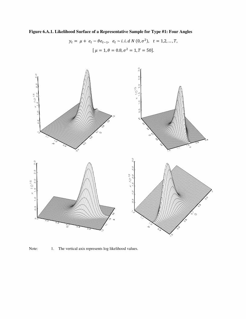
Figure 6.A.1. Likelihood Surface of a Representative Sample for Type #1: Four Angles ( ) [ ]
Note: 1. The vertical axis represents log likelihood values.

Figure 6.A.2. Comparison of Profile likelihood and Posterior Distribution for MA coefficient:
Representative Sample for Type #1 ( ) [ ]
Likelihood
Contour
Profile
Likelihood
Posterior
Distribution

Figure 6.B.1. Likelihood Surface of a Representative Sample for Type #2: Four Angles ( ) [ ]
Note: 2. The vertical axis represents log likelihood values.

Figure 6.B.2. Comparison of Profile likelihood and Posterior Distribution for MA coefficient:
Representative Sample for Type #2 ( ) [ ]
Likelihood
Contour
Profile
Likelihood
Posterior
Distribution

Figure 6.C.1. Likelihood Surface of a Representative Sample for Type #3: Four Angles ( ) [ ]
Note: 3. The vertical axis represents log likelihood values.

Figure 6.C.2. Comparison of Profile likelihood and Posterior Distribution for MA coefficient:
Representative Sample for Type #3 ( ) [ ]
Likelihood
Contour
Profile
Likelihood
Posterior
Distribution

Figure 7. Sampling Distributions of Bayesian Posterior Modes for θ: Monte Carlo Experiment
Model #1 (T=50) Model #1 (T=100) Model #1 (T=200)
Model #2 (T=50) Model #2 (T=100) Model #2 (T=200)
Model #3 (T=50) Model #3 (T=100) Model #3 (T=200)
Model #4 (T=50) Model #4 (T=100) Model #4 (T=200)
0.0
0.2
0.4
0.6
0.8
1.0
0.0 0.1 0.2 0.3 0.4 0.5 0.6 0.7 0.8 0.9 1.0
0.0
0.2
0.4
0.6
0.8
1.0
0.0 0.1 0.2 0.3 0.4 0.5 0.6 0.7 0.8 0.9 1.0
0.0
0.2
0.4
0.6
0.8
1.0
0.0 0.1 0.2 0.3 0.4 0.5 0.6 0.7 0.8 0.9 1.0
0.0
0.2
0.4
0.6
0.8
1.0
0.0 0.1 0.2 0.3 0.4 0.5 0.6 0.7 0.8 0.9 1.0
0.0
0.2
0.4
0.6
0.8
1.0
0.0 0.1 0.2 0.3 0.4 0.5 0.6 0.7 0.8 0.9 1.0
0.0
0.2
0.4
0.6
0.8
1.0
0.0 0.1 0.2 0.3 0.4 0.5 0.6 0.7 0.8 0.9 1.0
0.0
0.2
0.4
0.6
0.8
1.0
0.0 0.1 0.2 0.3 0.4 0.5 0.6 0.7 0.8 0.9 1.0
0.0
0.2
0.4
0.6
0.8
1.0
0.0 0.1 0.2 0.3 0.4 0.5 0.6 0.7 0.8 0.9 1.0
0.0
0.2
0.4
0.6
0.8
1.0
0.0 0.1 0.2 0.3 0.4 0.5 0.6 0.7 0.8 0.9 1.0
0.0
0.2
0.4
0.6
0.8
1.0
0.0 0.1 0.2 0.3 0.4 0.5 0.6 0.7 0.8 0.9 1.0
0.0
0.2
0.4
0.6
0.8
1.0
0.0 0.1 0.2 0.3 0.4 0.5 0.6 0.7 0.8 0.9 1.0
0.0
0.2
0.4
0.6
0.8
1.0
0.0 0.1 0.2 0.3 0.4 0.5 0.6 0.7 0.8 0.9 1.0
Note: 1. The total number of simulation is 5000.
2. The total number of Bayesian MCMC iteration is 6,000 and the first 1,000 samples are discarded.
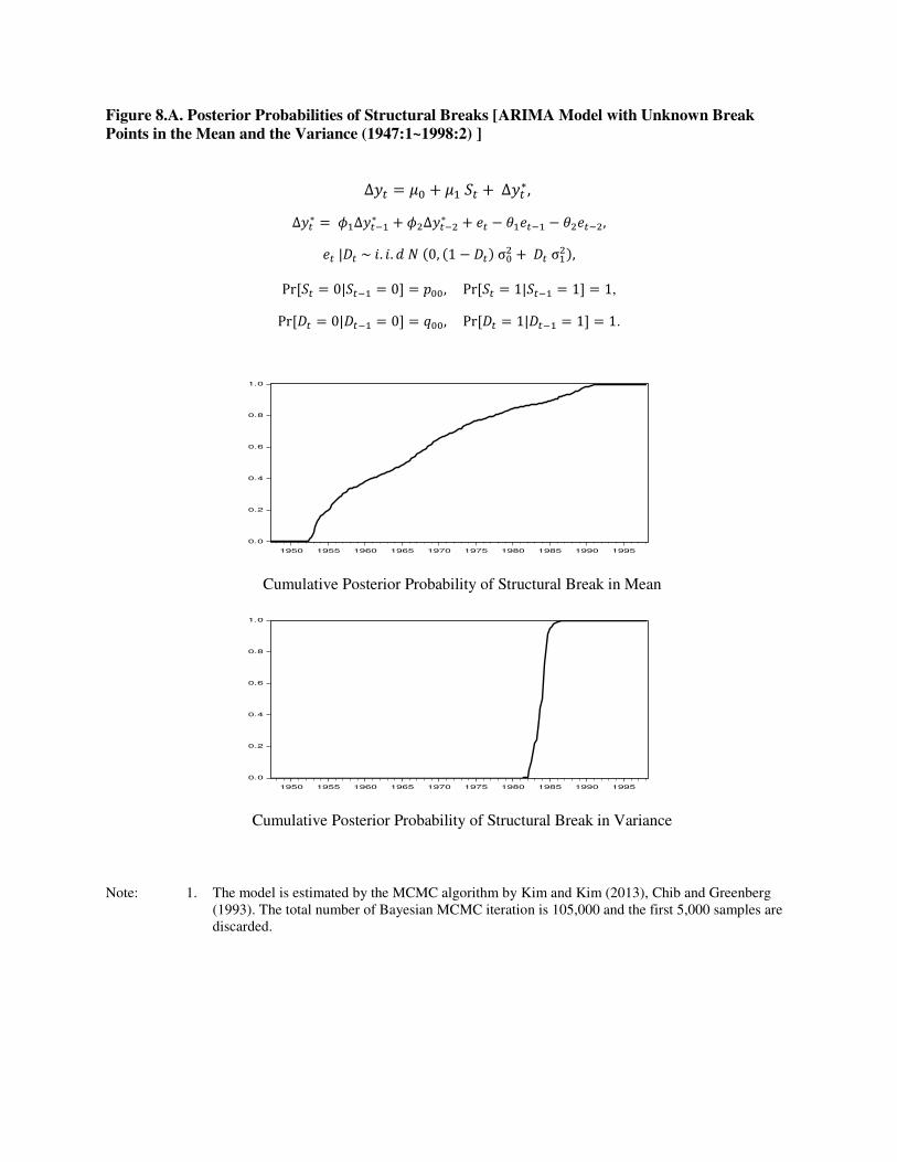
Figure 8.A. Posterior Probabilities of Structural Breaks [ARIMA Model with Unknown Break
Points in the Mean and the Variance (1947:1~1998:2) ]
( ( ) ) [ ] [ ] , [ ] [ ] .
Cumulative Posterior Probability of Structural Break in Mean
Cumulative Posterior Probability of Structural Break in Variance
Note: 1. The model is estimated by the MCMC algorithm by Kim and Kim (2013), Chib and Greenberg
(1993). The total number of Bayesian MCMC iteration is 105,000 and the first 5,000 samples are
discarded.
0.0
0.2
0.4
0.6
0.8
1.0
1950 1955 1960 1965 1970 1975 1980 1985 1990 1995
0.0
0.2
0.4
0.6
0.8
1.0
1950 1955 1960 1965 1970 1975 1980 1985 1990 1995
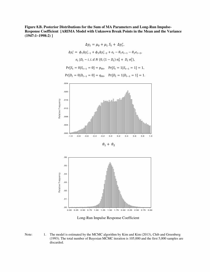
Figure 8.B. Posterior Distributions for the Sum of MA Parameters and Long-Run Impulse-
Response Coefficient [ARIMA Model with Unknown Break Points in the Mean and the Variance
(1947:1~1998:2) ] ( ( ) ) [ ] [ ] , [ ] [ ] .
Long-Run Impulse Response Coefficient
Note: 1. The model is estimated by the MCMC algorithm by Kim and Kim (2013), Chib and Greenberg
(1993). The total number of Bayesian MCMC iteration is 105,000 and the first 5,000 samples are
discarded.
.000
.004
.008
.012
.016
.020
.024
-1.0 -0.8 -0.6 -0.4 -0.2 0.0 0.2 0.4 0.6 0.8 1.0
Re
lati
ve
Fre
qu
en
cy
.00
.01
.02
.03
.04
.05
.06
0.00 0.25 0.50 0.75 1.00 1.25 1.50 1.75 2.00 2.25 2.50 2.75 3.00
Re
lati
ve
Fre
qu
en
cy

Figure 8.C. Trend-Cycle Decomposition and Impulse-Response Analysis [ARIMA Model with
Unknown Break Points in the Mean and the Variance (1947:1~1998:2) ]
( ( ) ) [ ] [ ] , [ ] [ ] .
Log of Real GDP vs. Trend Component
Cyclical Component
Impulse-Response Analysis
Note: 1. The model is estimated by the MCMC algorithm by Kim and Kim (2013), Chib and Greenberg
(1993). The total number of Bayesian MCMC iteration is 105,000 and the first 5,000 samples are
discarded.
720
760
800
840
880
920
1950 1955 1960 1965 1970 1975 1980 1985 1990 1995
Trend GDP
-8
-6
-4
-2
0
2
4
6
1950 1955 1960 1965 1970 1975 1980 1985 1990 1995
0.0
0.4
0.8
1.2
1.6
2.0
3 6 9 12 15 18 21 24 27 30
Top Related