


Languages
Pages
Legal

IntroductionUnknown boundary coefficient
Unknown boundaryAbnormal Diffusion
The Mathematical Analysis of
the Diffusion Process and its Applications
Cheng Jin
School of Mathematical Sciences, Fudan University
AIP09, Vienna, Austria
July 24th, 2009
Cheng Jin The Mathematical Analysis of

IntroductionUnknown boundary coefficient
Unknown boundaryAbnormal Diffusion
Outline
1 Introduction
2 Unknown boundary coefficient
Motivation and Modelling
Theoretic Results
Proof of the main results:
3 Unknown boundary
Motivation and Modelling
Forward Problems
Related Inverse Problems
4 Abnormal Diffusion
Related Inverse Problem
Cheng Jin The Mathematical Analysis of

IntroductionUnknown boundary coefficient
Unknown boundaryAbnormal Diffusion
Joint research with Masahiro Yamamoto(Tokyo
University, Japan), Shuai Lu (OCIAM, Austria), Wenbin
Chen, Xiaoyi Hu(Fudan University, China)
This research is partly supported by the Programme of
Introducing Talents of Discipline to Universities(No.B08018), the
NSFC (No.10431030), the Shuguang Project and E-Institute of
Shanghai Municipal Education Commission (N.E03004).
Cheng Jin The Mathematical Analysis of

IntroductionUnknown boundary coefficient
Unknown boundaryAbnormal Diffusion
We discuss the applications of the Mathematical Models of
Diffusion Process in the Industry and Environments Sciences,
Especially the methods of Inverse Problems.
Mathematical models:
Normal Diffusion: (Temperature Distribution in the steel)
Abnormal Diffusion: (Diffusion in the porous media)
Cheng Jin The Mathematical Analysis of
IntroductionUnknown boundary coefficient
Unknown boundaryAbnormal Diffusion
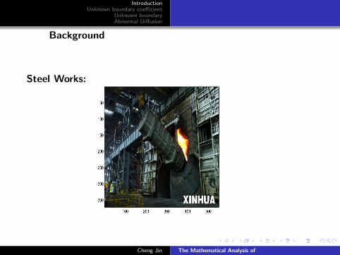
Background
Steel Works:
Cheng Jin The Mathematical Analysis of

IntroductionUnknown boundary coefficient
Unknown boundaryAbnormal Diffusion
Math is needed to produce steel safely and effectively, specially
PDE and ”inverse” PDE.
Cheng Jin The Mathematical Analysis of

IntroductionUnknown boundary coefficient
Unknown boundaryAbnormal Diffusion
Steel? Heat? Heat equation?
∂u
∂t−∆u = f (1)
It is so easy, just ask junior undergraduate students to code,
everything has been solved, I am happy:)
Cheng Jin The Mathematical Analysis of

IntroductionUnknown boundary coefficient
Unknown boundaryAbnormal Diffusion
Wait a moment:
Radiation interface conditions: Nonlinear
To detect the corrosion: Inverse problems
Requirement from the industry: High temperature, safe,
detection, ...
Math can be manufactured?
Minutes Days Weeks Months
Cheng Jin The Mathematical Analysis of

IntroductionUnknown boundary coefficient
Unknown boundaryAbnormal Diffusion
The modelling of the dynamics of anomalous processes by
means of differential equations that involve derivatives of fractional
order has provided interesting results in a variety of fields of
science. The most studied and applied model is the fractional
diffusion equations (FDE) which play an important role in
describing anomalous diffusion. A general account of FDEs is given
in R. Metzler and J. Klafter, Phys. Rep. 339, 1 (2000)
Cheng Jin The Mathematical Analysis of

IntroductionUnknown boundary coefficient
Unknown boundaryAbnormal Diffusion
Part I
Inverse Problems of Determining the unknownboundary in the heat process:
Cheng Jin The Mathematical Analysis of

IntroductionUnknown boundary coefficient
Unknown boundaryAbnormal Diffusion
We want to detect the defects in the thin sheetduring the steel rolling process by the thermalimage:
Cheng Jin The Mathematical Analysis of
IntroductionUnknown boundary coefficient
Unknown boundaryAbnormal Diffusion
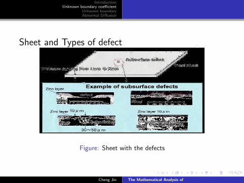
Sheet and Types of defect
Figure: Sheet with the defects
Cheng Jin The Mathematical Analysis of

IntroductionUnknown boundary coefficient
Unknown boundaryAbnormal Diffusion
Mathematical formulation of the problem:We consider the following mathematical model problem in the
heat transfer:
∂u
∂t= ∆u, 0 < t < T , x ∈ Ω (2)
−∂u
∂ν= σ(u4 − u4
A), 0 < t < T , x ∈ ∂Ω (3)
u = a(x), t = 0, x ∈ Ω (4)
where Ω is a simply connected domain in Rn with the C 2 boundary
∂Ω and ν is the outer normal unit with respect to ∂Ω.
Cheng Jin The Mathematical Analysis of

IntroductionUnknown boundary coefficient
Unknown boundaryAbnormal Diffusion
Here u represents the temperature distribution and uA is the
air temperature, which is assumed to be a positive constant.
σ(x) ∈ H2(∂Ω) is called the Stefan-Boltzmann radiation
coefficient, which characters the heat transfer between the solid
and air.
Cheng Jin The Mathematical Analysis of

IntroductionUnknown boundary coefficient
Unknown boundaryAbnormal Diffusion
Figure: Thermal Image
Cheng Jin The Mathematical Analysis of

IntroductionUnknown boundary coefficient
Unknown boundaryAbnormal Diffusion
Some assumptions on the domain:Suppose that the boundary ∂Ω can be divided as two parts Γ0
and Γ1, such that ∂Ω = Γ0 ∪ Γ1. Moreover, there is an one open
set ω ⊂ Γ1.
Cheng Jin The Mathematical Analysis of

IntroductionUnknown boundary coefficient
Unknown boundaryAbnormal Diffusion
The Assumptions on the coefficients
We assume that
(A1). uA is a given positive constant.
(A2). the Stenfan-Boltzmann coefficient σ ∈ C 2(∂Ω) and satisfies
σ(x) =
σ0, x ∈ Γ0 ∪ ω
γ(x), x ∈ Γ1 \ ω(5)
where σ0 is a given positive constant and γ is an unknown function.
(A3). The initial value a(x) > c0 > uA, where c0 is a given
constant.
Cheng Jin The Mathematical Analysis of

IntroductionUnknown boundary coefficient
Unknown boundaryAbnormal Diffusion
Our inverse problem is
find the unknown functions γ(x), x ∈ Γ1 and the initial value
a(x), x ∈ Ω from u(t, x), (t, x) ∈ (0,T )× Γ1.
The admissible set for the unknowns is
Λ =
(σ, a)
∣∣∣∣ ‖σ‖C2(∂Ω) ≤ M, σ > 0; ‖a‖C2(Ω) ≤ M, a(x) > c0
Cheng Jin The Mathematical Analysis of
IntroductionUnknown boundary coefficient
Unknown boundaryAbnormal Diffusion
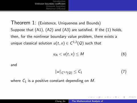
Theorem 1: (Existence, Uniqueness and Bounds)
Suppose that (A1), (A2) and (A3) are satisfied. If the (1) holds,
then, for the nonlinear boundary value problem, there exists a
unique classical solution u(t, x) ∈ C 1,2(Q) such that
uA < u(t, x) ≤ M (6)
and
‖u‖C1,2(Q) ≤ C1 (7)
where C1 is a positive constant depending on M.
Cheng Jin The Mathematical Analysis of

IntroductionUnknown boundary coefficient
Unknown boundaryAbnormal Diffusion
Theorem 2: (Uniqueness of IP)
Suppose that (σ1, a1), (σ2, a2) ∈ Λ and (A1), (A2) and (A3) are
satisfied. If it holds that
u1(t, x) = u2(t, x), 0 < t < T , x ∈ Γ1
then we have
σ1(x) = σ2(x), x ∈ ∂Ω
a1(x) = a2(x), x ∈ Ω.
Cheng Jin The Mathematical Analysis of

IntroductionUnknown boundary coefficient
Unknown boundaryAbnormal Diffusion
Theorem 3: (Conditional Stability of IP)
Suppose that (σ1, a1), (σ2, a2) ∈ Λ and (A1), (A2) and (A3) are
satisfied. Then, for the inverse problem we discuss, it holds that
‖σ1 − σ2‖C(∂Ω) ≤ C2‖(f1 − f2)esα‖C(Σ1) (8)
where fj(t, x) = uj(t, x), (t, x) ∈ Σ1 = (0,T )× Γ1, j = 1, 2, and
C2 is a positive constant depending on M and
η1 == min(t,x)∈(0,T )×∂Ω(u41 − u4
A).
α is defined in Carleman estimation and s(λ) > 0 is
sufficiently large for λ > λ, where λ > 0 depends on M.
Cheng Jin The Mathematical Analysis of

IntroductionUnknown boundary coefficient
Unknown boundaryAbnormal Diffusion
One Remark:
In Theorem 3, the Lipschitz stability estimation is only for the
unknown function σ. For another unknown function a(x), there is
also a conditional stability estimation results. It is a logarithmic
conditional stability estimation, which is too weak from the
numerical point of view.
Cheng Jin The Mathematical Analysis of

IntroductionUnknown boundary coefficient
Unknown boundaryAbnormal Diffusion
Definition of the weighted function
Suppose that ω is an open set in Γ1. Then there exits a function
ψ ∈ C 2(Ω) such that
ψ(x) > 0, x ∈ Ω, |∇ψ(x)| > 0, x ∈ Ω
ψ(x) = 0, x ∈ Γ0 ∪ ω,∂ψ
∂ν≤ 0, (t, x) ∈ [0,T ]× (∂Ω \ ω).
Cheng Jin The Mathematical Analysis of

IntroductionUnknown boundary coefficient
Unknown boundaryAbnormal Diffusion
Definition of the weighted function
Let
l(t) = t(T − t).
We set
φ(t, x) =eλψ(x)
l(t)(9)
and
α(t, x) =eλψ(x) − e
2λ‖ψ‖C(Ω)
l(t)(10)
where λ is a positive constant.
Cheng Jin The Mathematical Analysis of

IntroductionUnknown boundary coefficient
Unknown boundaryAbnormal Diffusion
The equationWe consider a function w ∈ W 1,2
2 (Q), which is a weak solution of
the following problem:
∂w∂t = ∆u + g(t, x), 0 < t < T , x ∈ Ω
∂w∂ν + k(t, x)w = 0, 0 < t < T , x ∈ Γ0
w = 0, < t < T , x ∈ Γ1
w = a, t = 0, x ∈ Ω.
(11)
Cheng Jin The Mathematical Analysis of

IntroductionUnknown boundary coefficient
Unknown boundaryAbnormal Diffusion
Carleman estimation: (Imanuvilov, Yamamoto )
Suppose that w is the weak solution of (11) and
‖k‖C((0,T )×Γ1), ‖∂k
∂t‖C((0,T )×Γ1) ≤ M1.
Then there exists a λ, which depends on M1, such that, for
any arbitrary λ ≥ λ, we can choose s0(λ) satisfying: for any
s ≥ s0(λ), the following estimation holds:
Cheng Jin The Mathematical Analysis of

IntroductionUnknown boundary coefficient
Unknown boundaryAbnormal Diffusion
∫Q
(sφ)p−1
∣∣∣∣∂w
∂t
∣∣∣∣2 +n∑
i ,j=1
∣∣∣∣ ∂2w
∂xi∂xj
∣∣∣∣2 e2sαdxdt
+
∫Q
((sφ)p+1|∇w |2 + (sφ)p+3w2
)e2sαdxdt
≤ C2
∫Q
(sφ)p|g |2e2sαdxdt + C2
∫(0,T )×ω
(sφ)p(∂w
∂t
)2
e2sαdxdt
+C2
∫(0,T )×ω
((sφ)p+1|∇w |2 + (sφ)p+3w2
)e2sαdxdt
where C2 is a positive constant depending λ.
Cheng Jin The Mathematical Analysis of

IntroductionUnknown boundary coefficient
Unknown boundaryAbnormal Diffusion
Outline of the proof of Theorem 3:
Step 1:
By Carleman estimation, we can prove that
‖u1 − u2‖L2((0,T )×Γ1\ω) + ‖∂(u1 − u2)
∂ν‖L2((0,T )×Γ1\ω)
≤ C‖(f1 − f2)e2sα‖
W 1,12 (0,T )×Γ1)
.
Cheng Jin The Mathematical Analysis of

IntroductionUnknown boundary coefficient
Unknown boundaryAbnormal Diffusion
Outline of the proof of Theorem 3:
Step 2:
By the nonlinear boundary condition, we have
∂u1
∂ν− ∂u1
∂ν= (σ1 − σ2)(u
41 − u4
A) + σ2(u41 − u4
2).
Cheng Jin The Mathematical Analysis of

IntroductionUnknown boundary coefficient
Unknown boundaryAbnormal Diffusion
Some remarks:
For the convenience of proving the results, we assume that
more regularity for the unknown functions. These assumptions can
be weakened by the same method.
Cheng Jin The Mathematical Analysis of
IntroductionUnknown boundary coefficient
Unknown boundaryAbnormal Diffusion
Some remarks:
The numerical methods based on our analysis for the inverse
problems have been proposed. The reader can find the related
results in the forthcoming paper from our group.
Cheng Jin The Mathematical Analysis of
IntroductionUnknown boundary coefficient
Unknown boundaryAbnormal Diffusion
Future works:
1 The case σ is a piecewise smooth function.
2 Multi-layers cases (reduce the measurements)
3 Other applications
Cheng Jin The Mathematical Analysis of

IntroductionUnknown boundary coefficient
Unknown boundaryAbnormal Diffusion
Part II
Inverse Problems of Determining the unknownboundary:
Cheng Jin The Mathematical Analysis of

IntroductionUnknown boundary coefficient
Unknown boundaryAbnormal Diffusion
We want to describe the temperature distributioninside the container in the process of continuouscasting:
Cheng Jin The Mathematical Analysis of
IntroductionUnknown boundary coefficient
Unknown boundaryAbnormal Diffusion
The governing equations are the heat equation
∂u
∂t= a∆u, inside the layers
Cheng Jin The Mathematical Analysis of
IntroductionUnknown boundary coefficient
Unknown boundaryAbnormal Diffusion
The heat transfer on the interfaces:1 The heat transfer between the outer layer and air
2 The heat transfer between the different layers
3 The heat transfer between the inner layer and molten steel
Cheng Jin The Mathematical Analysis of

IntroductionUnknown boundary coefficient
Unknown boundaryAbnormal Diffusion
Cheng Jin The Mathematical Analysis of
IntroductionUnknown boundary coefficient
Unknown boundaryAbnormal Diffusion
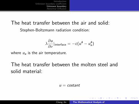
The heat transfer between the air and solid:Stephen-Boltzmann radiation condition:
λ∂u
∂ν|interface = −c(u4 − u4
a)
where ua is the air temperature.
The heat transfer between the molten steel andsolid material:
u = costant
Cheng Jin The Mathematical Analysis of

IntroductionUnknown boundary coefficient
Unknown boundaryAbnormal Diffusion
How to model the heat transfer between the different layers?
Previous Formulation:
u+ = u−, λ+∂u+
∂ν= λ−
∂u−
∂ν, on interface
This is not consistent with the experimentresults!
On the interface, the temperatures on the different layers are
different. i.e.
u+ 6= u−, on interface
Cheng Jin The Mathematical Analysis of

IntroductionUnknown boundary coefficient
Unknown boundaryAbnormal Diffusion
We consider the case
λ+∂u+
∂ν= −c((u+)4 − u4
∗)
λ−∂u−
∂ν= c((u−)4 − u4
∗)
Let δ → 0Cheng Jin The Mathematical Analysis of

IntroductionUnknown boundary coefficient
Unknown boundaryAbnormal Diffusion
We have the transmission conditions on the interface:
λ+∂u+
∂ν= λ−
∂u−
∂ν
λ+∂u+
∂ν= −c
2((u+)4 − (u−)4)
Nonlinear Transmission conditions!
Cheng Jin The Mathematical Analysis of

IntroductionUnknown boundary coefficient
Unknown boundaryAbnormal Diffusion
We consider the one dimensional case
∂tu1(x , t) = α1∂2xu1(x , t), 0 < x < `1, 0 < t < T ,
∂tu2(x , t) = α2∂2xu2(x , t), `1 < x < `2, 0 < t < T ,
∂tu3(x , t) = α3∂2xu3(x , t), `2 < x < `3, 0 < t < T ,
with an initial condition:
u(x , 0) = a(x), 0 < x < `3Cheng Jin The Mathematical Analysis of
IntroductionUnknown boundary coefficient
Unknown boundaryAbnormal Diffusion
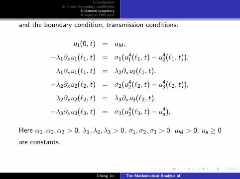
and the boundary condition, transmission conditions:
u1(0, t) = uM ,
−λ1∂xu1(`1, t) = σ1(u41(`1, t)− u4
2(`1, t)),
λ1∂xu1(`1, t) = λ2∂xu2(`1, t),
−λ2∂xu2(`2, t) = σ2(u42(`2, t)− u4
3(`2, t)),
λ2∂xu2(`2, t) = λ3∂xu3(`2, t),
−λ3∂xu3(`3, t) = σ3(u43(`3, t)− u4
a),
Here α1, α2, α3 > 0, λ1, λ2, λ3 > 0, σ1, σ2, σ3 > 0, uM > 0, ua ≥ 0
are constants.
Cheng Jin The Mathematical Analysis of

IntroductionUnknown boundary coefficient
Unknown boundaryAbnormal Diffusion
We have the result:Theorem: Suppose that a(x) satisfies the compatibility
conditions. Let T be arbitrarily given. Then there exists a unique
solution.
The solutions are within the class:u1 ∈ C1([0,T ];C2[0, `1]),
u2 ∈ C1([0,T ];C2[`1, `2]),
u3 ∈ C1([0,T ];C2[`2, `3]),
(12)
Cheng Jin The Mathematical Analysis of
IntroductionUnknown boundary coefficient
Unknown boundaryAbnormal Diffusion
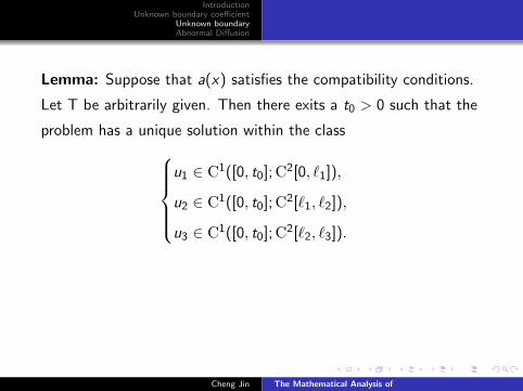
Lemma: Suppose that a(x) satisfies the compatibility conditions.
Let T be arbitrarily given. Then there exits a t0 > 0 such that the
problem has a unique solution within the classu1 ∈ C1([0, t0];C2[0, `1]),
u2 ∈ C1([0, t0];C2[`1, `2]),
u3 ∈ C1([0, t0];C2[`2, `3]).
Cheng Jin The Mathematical Analysis of
IntroductionUnknown boundary coefficient
Unknown boundaryAbnormal Diffusion
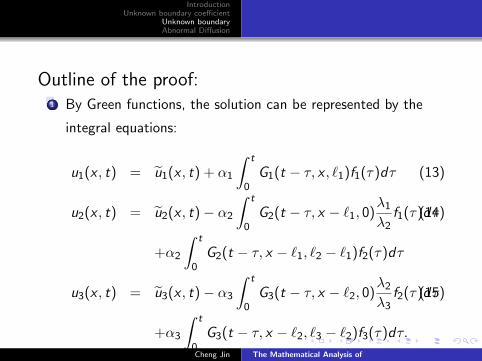
Outline of the proof:1 By Green functions, the solution can be represented by the
integral equations:
u1(x , t) = u1(x , t) + α1
∫ t
0G1(t − τ, x , `1)f1(τ)dτ (13)
u2(x , t) = u2(x , t)− α2
∫ t
0G2(t − τ, x − `1, 0)
λ1
λ2f1(τ)dτ(14)
+α2
∫ t
0G2(t − τ, x − `1, `2 − `1)f2(τ)dτ
u3(x , t) = u3(x , t)− α3
∫ t
0G3(t − τ, x − `2, 0)
λ2
λ3f2(τ)dτ(15)
+α3
∫ t
0G3(t − τ, x − `2, `3 − `2)f3(τ)dτ.
Cheng Jin The Mathematical Analysis of
IntroductionUnknown boundary coefficient
Unknown boundaryAbnormal Diffusion
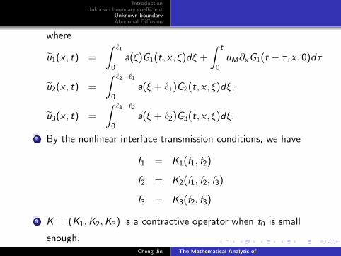
where
u1(x , t) =
∫ `1
0a(ξ)G1(t, x , ξ)dξ +
∫ t
0uM∂xG1(t − τ, x , 0)dτ
u2(x , t) =
∫ `2−`1
0a(ξ + `1)G2(t, x , ξ)dξ,
u3(x , t) =
∫ `3−`2
0a(ξ + `2)G3(t, x , ξ)dξ.
2 By the nonlinear interface transmission conditions, we have
f1 = K1(f1, f2)
f2 = K2(f1, f2, f3)
f3 = K3(f2, f3)
3 K = (K1,K2,K3) is a contractive operator when t0 is small
enough.Cheng Jin The Mathematical Analysis of

IntroductionUnknown boundary coefficient
Unknown boundaryAbnormal Diffusion
Lemma: Suppose that there exists the solution u1, u2, u3 and
a > 0, uM > ua > 0 . Then we have
u1(`1, t) > 0, u2(`1, t) > 0, u2(`2, t) > 0,
u3(`2, t) > 0, u3(`3, t) > 0, for t > 0.
Lemma: Suppose that there exists the solution u1, u2, u3 and let
T > 0 be arbitrarily fixed. Then it holds that
max‖u1‖C([0,`1]×[0,T ]), ‖u2‖C([`1,`2]×[0,T ]), ‖u3‖C([`2,`3]×[0,T ])
≤ max‖a‖C [0,`3], |uM |, |ua|.
Cheng Jin The Mathematical Analysis of
IntroductionUnknown boundary coefficient
Unknown boundaryAbnormal Diffusion
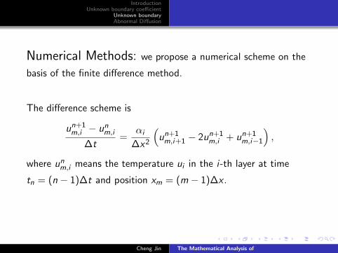
Numerical Methods: we propose a numerical scheme on the
basis of the finite difference method.
The difference scheme is
un+1m,i − un
m,i
∆t=
αi
∆x2
(un+1m,i+1 − 2un+1
m,i + un+1m,i−1
),
where unm,i means the temperature ui in the i-th layer at time
tn = (n − 1)∆t and position xm = (m − 1)∆x .
Cheng Jin The Mathematical Analysis of
IntroductionUnknown boundary coefficient
Unknown boundaryAbnormal Diffusion
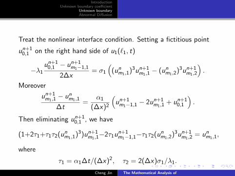
Treat the nonlinear interface condition. Setting a fictitious point
un+10,1 on the right hand side of u1(`1, t)
−λ1
un+10,1 − un+1
m1−1,1
2∆x= σ1
((un
m1,1)3un+1
m1,1− (un
m1,2)3un+1
m1,2
).
Moreover
un+1m1,1
− unm1,1
∆t=
α1
(∆x)2
(un+1m1−1,1 − 2un+1
m1,1+ un+1
0,1
).
Then eliminating un+10,1 , we have
(1+2τ1+τ1τ2(unm1,1)
3)un+1m1,1
−2τ1un+1m1−1,1−τ1τ2(u
nm1,2)
3un+1m1,2
= unm1,1,
where
τ1 = α1∆t/(∆x)2, τ2 = 2(∆x)σ1/λ1.
Cheng Jin The Mathematical Analysis of

IntroductionUnknown boundary coefficient
Unknown boundaryAbnormal Diffusion
Numerical Simulations:Setting uM = 1873, a(x) ≡ 303 and the parameters are
chosen as:α1 = 4.02× 10⁻², λ1 = 40, σ1 = 4.88× 10⁻⁴, `1 = 0.06,
α2 = 1.7× 10⁻³, λ2 = 1.2, σ2 = 4.88× 10⁻⁴, `2 − `1 = 0.1,
α3 = 9.3× 10⁻³, λ3 = 7.3, σ3 = 4.88× 10⁻⁴, `3 − `2 = 0.04.
Cheng Jin The Mathematical Analysis of

IntroductionUnknown boundary coefficient
Unknown boundaryAbnormal Diffusion
The numerical results under the grid: ∆t = 0.001,∆x = 0.001 are
shown in Figure 1 and Figure 2 for T = 0.02 hour and T = 0.1
hour:
Cheng Jin The Mathematical Analysis of

IntroductionUnknown boundary coefficient
Unknown boundaryAbnormal Diffusion
Cheng Jin The Mathematical Analysis of
IntroductionUnknown boundary coefficient
Unknown boundaryAbnormal Diffusion
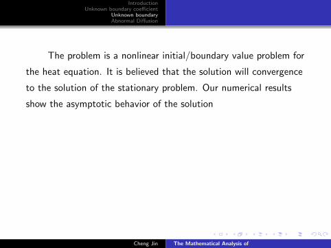
The problem is a nonlinear initial/boundary value problem for
the heat equation. It is believed that the solution will convergence
to the solution of the stationary problem. Our numerical results
show the asymptotic behavior of the solution
Cheng Jin The Mathematical Analysis of
IntroductionUnknown boundary coefficient
Unknown boundaryAbnormal Diffusion
Cheng Jin The Mathematical Analysis of

IntroductionUnknown boundary coefficient
Unknown boundaryAbnormal Diffusion
Cheng Jin The Mathematical Analysis of

IntroductionUnknown boundary coefficient
Unknown boundaryAbnormal Diffusion
Purpose: Detect the corrosion inside from the thermal image
outside.
Based on the forward model!
Cheng Jin The Mathematical Analysis of

IntroductionUnknown boundary coefficient
Unknown boundaryAbnormal Diffusion
The part which contains some corrosion:
Cheng Jin The Mathematical Analysis of

IntroductionUnknown boundary coefficient
Unknown boundaryAbnormal Diffusion
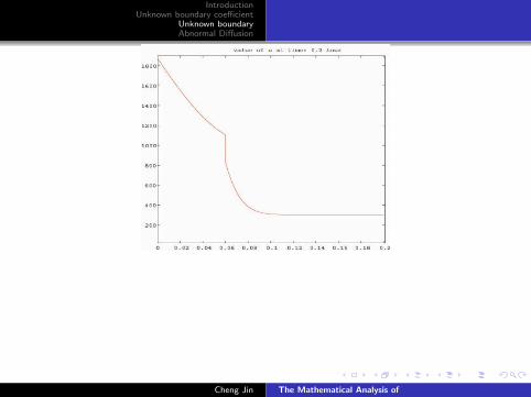
The temperature distribution outside
Cheng Jin The Mathematical Analysis of
IntroductionUnknown boundary coefficient
Unknown boundaryAbnormal Diffusion
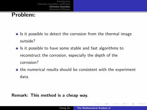
Problem:
Is it possible to detect the corrosion from the thermal image
outside?
Is it possible to have some stable and fast algorithms to
reconstruct the corrosion, especially the depth of the
corrosion?
the numerical results should be consistent with the experiment
data.
Remark: This method is a cheap way.
Cheng Jin The Mathematical Analysis of
IntroductionUnknown boundary coefficient
Unknown boundaryAbnormal Diffusion
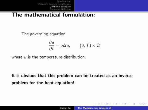
The mathematical formulation:
The governing equation:
∂u
∂t= a∆u, (0,T )× Ω
where u is the temperature distribution.
It is obvious that this problem can be treated as an inverse
problem for the heat equation!
Cheng Jin The Mathematical Analysis of
IntroductionUnknown boundary coefficient
Unknown boundaryAbnormal Diffusion
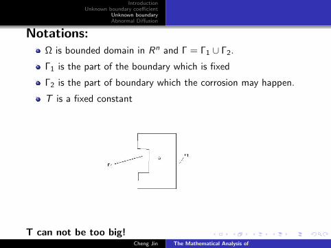
Notations:Ω is bounded domain in Rn and Γ = Γ1 ∪ Γ2.
Γ1 is the part of the boundary which is fixed
Γ2 is the part of boundary which the corrosion may happen.
T is a fixed constant
T can not be too big!Cheng Jin The Mathematical Analysis of

IntroductionUnknown boundary coefficient
Unknown boundaryAbnormal Diffusion
The mathematical formulation:
∂u
∂t= α∆u, (0,T )× Ω
u = c0, (0,T )× Γ2
∂u
∂ν= c(u4 − u4
a), (0,T )× Γ1
The additional data is given
u = f , (0,T )× Γ1
Cheng Jin The Mathematical Analysis of
IntroductionUnknown boundary coefficient
Unknown boundaryAbnormal Diffusion
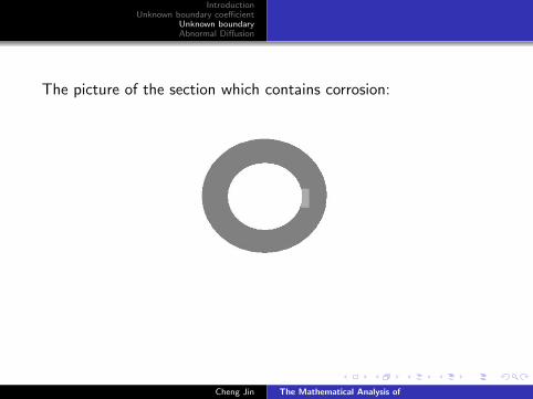
The picture of the section which contains corrosion:
Cheng Jin The Mathematical Analysis of

IntroductionUnknown boundary coefficient
Unknown boundaryAbnormal Diffusion
We will study:
1 The additional information is enough to determine the
unknown boundary? (Uniqueness)
2 If so, is it possible to give a fast and stable reconstruction
algorithm?
Cheng Jin The Mathematical Analysis of

IntroductionUnknown boundary coefficient
Unknown boundaryAbnormal Diffusion
Difficulties:
1 ill-posedness: Cauchy problem for heat equation
2 no initial data
3 T is not so big
Cheng Jin The Mathematical Analysis of
IntroductionUnknown boundary coefficient
Unknown boundaryAbnormal Diffusion
Previous work on this topic:
Transform to an optimization problem!
not so good!
Cheng Jin The Mathematical Analysis of

IntroductionUnknown boundary coefficient
Unknown boundaryAbnormal Diffusion
Theoretic analysis: (one dimensional model)
Ω = (0, l), Γ1 = 0, Γ2 = l
∂u
∂t=∂2u
∂x2, 0 < x < l , 0 < t < T
u(t, 0) = f (t), 0 < t < T
∂u
∂x(t, 0) = g(t), 0 < t < T
u(t, l) = c0, 0 < t < T
Cheng Jin The Mathematical Analysis of
IntroductionUnknown boundary coefficient
Unknown boundaryAbnormal Diffusion
Uniqueness Results:
Suppose that T = ∞, ‖f ‖C2 ≤ M and ‖g‖C2 ≤ M. Assume
that there exists a constant γ0 > 0 such that
‖f − c0‖ ≥ γ0
If, for two l , l , the solutions u and u satisfy the previous equations
and boundary conditions, then we have l = l .
Cheng Jin The Mathematical Analysis of

IntroductionUnknown boundary coefficient
Unknown boundaryAbnormal Diffusion
Outline of the proof:
Assume that l < l .
1 By the uniqueness of the Cauchy problem for heat equation,
we can conclude
u(x , t) = u(x , t), 0 < x < l , 0 < t < T .
2 We have that
∂u
∂t=∂2u
∂x2, l < x < l , 0 < t < T
u(t, l) = c0, 0 < t < T
u(t, l) = c0, 0 < t < TCheng Jin The Mathematical Analysis of

IntroductionUnknown boundary coefficient
Unknown boundaryAbnormal Diffusion
3 By the result for the heat equation, it holds that
‖u − c0‖C(l ,l) −→ 0, t →∞.
4 By the unique continuation for the heat equation, we have
that
|u(t, 0)− c0| → 0, t →∞
This is the contradiction to our assumption!
Cheng Jin The Mathematical Analysis of
IntroductionUnknown boundary coefficient
Unknown boundaryAbnormal Diffusion
Remarks:
The contribution of the initial data is not important
This result is true for multidimensional cases
The conditional stability can be obtained.
(The several conditional stability results of the inverse problem
for the parabolic equations with the given initial condition
have obtained by the Italy group and other researchers.)
Cheng Jin The Mathematical Analysis of

IntroductionUnknown boundary coefficient
Unknown boundaryAbnormal Diffusion
Numerical Algorithm:We consider
∂u∂t = ∂2u
∂x2 , 0 < x < l , 0 < t < T
u(t, 0) = f1(t), 0 < t < T
u(t, l) = f2(t), 0 < t < T
∂u∂x (t, 0) = h(t), 0 < t < T
∂u∂x (t, l) = g(t), 0 < t < T
u(0, x) = u0(x)
Cheng Jin The Mathematical Analysis of

IntroductionUnknown boundary coefficient
Unknown boundaryAbnormal Diffusion
Let
G (t, x , y) =2
l
∞∑n=0
e−λnt sin(n +1
2)π
lx sin(n +
1
2)π
ly
Then the solution can be expressed by
u(t, x) =∞∑
n=0
Ane−λnt sin(n +
1
2)π
lx +
∫ t
0
∂G
∂x(t − s, x , 0)f1(s)ds
+
∫ t
0G (t − s, x , l)g(s)ds, 0 < x < l , 0 < t < T
Cheng Jin The Mathematical Analysis of

IntroductionUnknown boundary coefficient
Unknown boundaryAbnormal Diffusion
Evaluate:Let
w(t, x) =
∫ tj
ti
∂G
∂x(t − s, x , 0)ds
It satisfies
∂w∂t = ∂2w
∂x2 , 0 < x < l , 0 < t < T
w(0, x) = 0
∂w∂x (t, l) = 0
w(t, 0) =
1, t ∈ [ti , tj ]
0, otherwiae
Cheng Jin The Mathematical Analysis of

IntroductionUnknown boundary coefficient
Unknown boundaryAbnormal Diffusion
Numerical Algorithm:
1 First, we fix a suitable initial data and choose a l0 By the
formula, we can solve the forward problem and obtain∂u0∂x (t, 0).
2 Compare u0∂x (t, 0) with h(t) for t > T1 and choose another l1.
Goto Step 1
3 Stopping criteria:
‖∂u0
∂x(t, 0)− h(t)‖ ≤ ε, for t > T1
Cheng Jin The Mathematical Analysis of

IntroductionUnknown boundary coefficient
Unknown boundaryAbnormal Diffusion
Key Point:
At each step, we just compare the numerical results with the
data for t > T1, i.e.
‖∂u0
∂x(t, 0)− h(t)‖ ≤ ε, for t > T1
Cheng Jin The Mathematical Analysis of

IntroductionUnknown boundary coefficient
Unknown boundaryAbnormal Diffusion
Numerical results:
Cheng Jin The Mathematical Analysis of

IntroductionUnknown boundary coefficient
Unknown boundaryAbnormal Diffusion
Future works:
1 Multi-dimensional case (fast algorithm)
2 Multi-layers cases (reduce the measurements)
3 Other applications
Cheng Jin The Mathematical Analysis of
IntroductionUnknown boundary coefficient
Unknown boundaryAbnormal Diffusion
Part III
One Inverse Problem Example in FractionalDiffusion:
Cheng Jin The Mathematical Analysis of

IntroductionUnknown boundary coefficient
Unknown boundaryAbnormal Diffusion
.
Consider a periodically kicked rotator whose dynamical
equation is generated by the following Hamiltonian:
H =p2
2− K cos(x)
∞∑m=−∞
δ(t −m)
Assume that m ∈ N, then it can be rewritten as:
pn+1 = pn + K sin(xn)
xn+1 = xn + pn+1
There is a critical value Kc ≈ 0.97 for this kicked rotator, and
if K ≤ Kc the phase space is regular otherwise the chaos will
appear.Cheng Jin The Mathematical Analysis of

IntroductionUnknown boundary coefficient
Unknown boundaryAbnormal Diffusion
Greene, J.M., A method for determining a stochastic transition .
1979. J. Math. Phys. 20, 1183-1201.
Cheng Jin The Mathematical Analysis of

IntroductionUnknown boundary coefficient
Unknown boundaryAbnormal Diffusion
The following figure called stochastic sea shows the phase
space (p, x) with different initial conditions with K = 1.1.
Figure: Strange Kinetics, Nature, May 6, 1993.
Cheng Jin The Mathematical Analysis of

IntroductionUnknown boundary coefficient
Unknown boundaryAbnormal Diffusion
This new topological object in phase space (p, x) called
cantorus has some properties
A closed curve except for an infinite number of gaps
The measure of cantorus is zero.
Particles can pass through the gaps
The particle gets trapped inside the area between the island
border and nearest cantorus.
This is why one can observe high densities of dots in the stochastic
sea.
Cheng Jin The Mathematical Analysis of

IntroductionUnknown boundary coefficient
Unknown boundaryAbnormal Diffusion
Once the particle was trapped between the border of islands
and the nearest cantorus, the (Mean Squared Displacement) will
behavior as ⟨x2(t)− 〈x(t)〉2
⟩= Dt2µ
where µ < 1/2.
Sometimes µ > 1/2, which is corresponding to strong
enhancement of transport (ballistic or jet motion). This
phenomenon can be observed in plasma fusion and spread of
environmental pollution and etc.
To Describe these phenomenons we need turn to
fractional diffusion equation!
Cheng Jin The Mathematical Analysis of

IntroductionUnknown boundary coefficient
Unknown boundaryAbnormal Diffusion
In order to describe the abnormal diffusion in inhomogeneous
media a new time fractional diffusion equation whose order varies
with space proposed by A.V. Chechkin using CTRW.
∂p(x , t)
∂t=
∂2
∂x2
(K (x)D
1−β(x)t p(x , t)
),
where
D1−β(x)t p(x , t) :=
1
Γ(β(x))
∂
∂t
∫ t
0
p(x , τ)
(t − τ)1−β(x)dτ
Cheng Jin The Mathematical Analysis of

IntroductionUnknown boundary coefficient
Unknown boundaryAbnormal Diffusion
For simplicity we assume that the media are composite of two
kinds of different materials, i.e.,
K (x) =
K+, x > 0
K−, x < 0.β(x) =
β+, x > 0
β−, x < 0.
p(±∞, t) = 0 and p(x , 0) = f (x). Performing the Laplace
transformation of and considering the initial/boundary condition
gives:
p±(x , s) =
∫ +∞
−∞
exp(− |x−ξ|sv±√
K±
)s(√
K+s−v+ +√
K−s−v−) f (ξ)dξ
where v± =β±2
.
Cheng Jin The Mathematical Analysis of
IntroductionUnknown boundary coefficient
Unknown boundaryAbnormal Diffusion
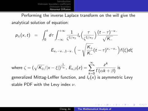
Performing the inverse Laplace transform on the will give the
analytical solution of equation:
p±(x , t) =
∫ t
0dτ
∫ +∞
−∞
1
ζ1/v±lv( τ
ζ1/v±
)(t − τ)−v−√K−
Ev+−v−,1−v−
(−
√K+
K−(t − τ)v+−v−
)f (ξ)dξ
where ζ = (√
K±/|x − ξ|)1
v± , Eα,β(z) =∞∑
k=0
zk
Γ(αk + β)is
generalized Mittag-Leffler function, and lv (x) is asymmetric Levy
stable PDF with the Levy index ν.
Cheng Jin The Mathematical Analysis of
IntroductionUnknown boundary coefficient
Unknown boundaryAbnormal Diffusion
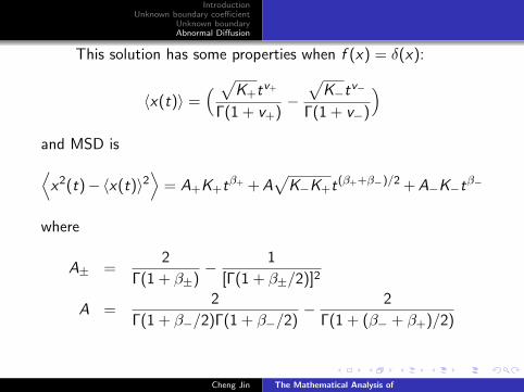
This solution has some properties when f (x) = δ(x):
〈x(t)〉 =( √K+tv+
Γ(1 + v+)−√
K−tv−
Γ(1 + v−)
)and MSD is⟨x2(t)−〈x(t)〉2
⟩= A+K+tβ+ + A
√K−K+t(β++β−)/2 + A−K−tβ−
where
A± =2
Γ(1 + β±)− 1
[Γ(1 + β±/2)]2
A =2
Γ(1 + β−/2)Γ(1 + β−/2)− 2
Γ(1 + (β− + β+)/2)
Cheng Jin The Mathematical Analysis of

IntroductionUnknown boundary coefficient
Unknown boundaryAbnormal Diffusion
We use Grunwald-Letnikow formula to approximate the
fractional derivatives, that is,
D1−β(x)t p = lim
∆t→0
1
∆t1−β(x)
[ t∆t
]∑k=0
(−1)k
(1− β(x)
k
)p(x , t − k∆t)
In fact we replace p(x , t − k∆t) by p(x , t − (k − 1)∆t) to avoid
unstability in computation. And the interface condition is:
p(0+, t) = p(0−, t)
K (0+)d
dxD
1−β(0+)t p(0+, t) = K (0−)
d
dxD
1−β(0−)t p(0−, t)
Cheng Jin The Mathematical Analysis of

IntroductionUnknown boundary coefficient
Unknown boundaryAbnormal Diffusion
Figure 1. The former one shows numerical solution of normal diffusion.
The latter one displays the numerical solution of fractional diffusion with
β+ = 1, β− = 0.8, K+ = 1.2 and K− = 1.
Cheng Jin The Mathematical Analysis of
IntroductionUnknown boundary coefficient
Unknown boundaryAbnormal Diffusion
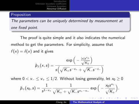
Proposition
The parameters can be uniquely determined by measurement at
one fixed point.
The proof is quite simple and it also indicates the numerical
method to get the parameters. For simplicity, assume that
f (x) = δ(x) and it gives
p±(x , s) =exp
(− |x |sv±√
K±
)s(√
K+s−v+ +√
K−s−v−)
where 0 < v− ≤ v+ ≤ 1/2. Without losing generality, let x0 ≥ 0
p+(x0, s) =1
s1−v+
1√K+ +
√K−sv+−v−
exp(− x0s
v+√K+
).
Cheng Jin The Mathematical Analysis of

IntroductionUnknown boundary coefficient
Unknown boundaryAbnormal Diffusion
Then
lims→0
sµp+(x0, s) =
0, µ > 1− v+
1√K+
, µ = 1− v+.
∞, µ < 1− v+.
So by choosing different µ, we can determine v+ and K+. Then,
let s = 1, then
p+(x0, 1) =1√
K+ +√
K−exp
(− x0√
K+
)and by algebraic computation we can get
K− =
(1
p+(x0, 1)exp
(− x0√
K+
)−√
K+
)2
.
Cheng Jin The Mathematical Analysis of
IntroductionUnknown boundary coefficient
Unknown boundaryAbnormal Diffusion
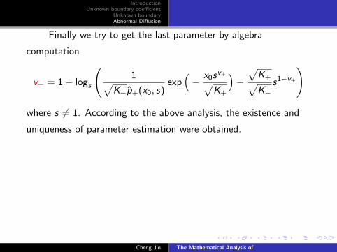
Finally we try to get the last parameter by algebra
computation
v− = 1− logs
(1√
K−p+(x0, s)exp
(− x0s
v+√K+
)−√
K+√K−
s1−v+
)
where s 6= 1. According to the above analysis, the existence and
uniqueness of parameter estimation were obtained.
Cheng Jin The Mathematical Analysis of

IntroductionUnknown boundary coefficient
Unknown boundaryAbnormal Diffusion
In practice we usually turn to Tikhonov regularization method
to recover unknown parameters, i.e.,
β(x),K (x) = argmin ‖p(x0, s)−pε(x0, s)‖+α1‖β(x)‖+α2‖K (x)‖
where pε(x0, s) = L[pε(x0, t)], and pε(x0, t) is the data with error.
α1 and α2 are regularization parameters.
Cheng Jin The Mathematical Analysis of

IntroductionUnknown boundary coefficient
Unknown boundaryAbnormal Diffusion
Consider the simple case of K and β, we choose
α1 = α2 = 0, and pε given by the numerical solution which
obtained before where ε = O(∆x + ∆t). The final result is
β+ = 1.0000, β− = 0.9539, K+ = 0.9702 and K− = 0.9343.
(exact value β± = K± = 1)
β+ = 0.9949, β− = 0.8425, K+ = 1.1764 and K− = 0.9144.
(exact value β+ = 1, β− = 0.8,K+ = 1.2,K− = 1.)
Cheng Jin The Mathematical Analysis of
IntroductionUnknown boundary coefficient
Unknown boundaryAbnormal Diffusion
Thank You!!!
Cheng Jin The Mathematical Analysis of

IntroductionUnknown boundary coefficient
Unknown boundaryAbnormal Diffusion
International Conference on Inverse Problems
April 26th – 29th, 2010, Wuhan, China
http://www.math.cuhk.edu.hk/special/icip2010/
Cheng Jin The Mathematical Analysis of
Top Related