


Languages
Pages
Legal

The Laplace Transform
www.asyrani.com

INTRODUCTION
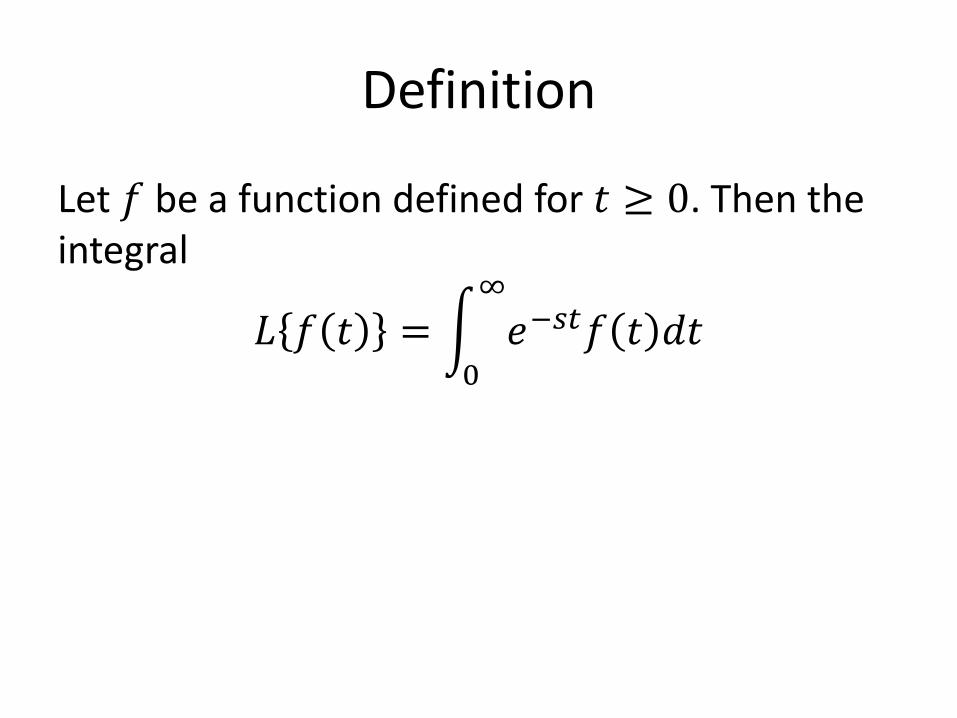
Definition
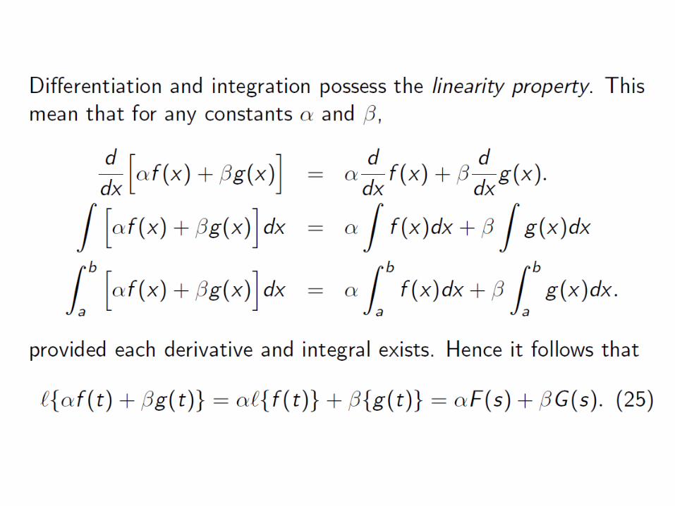
Let 𝑓 be a function defined for 𝑡 ≥ 0. Then the integral
𝐿 𝑓 𝑡 = 𝑒−𝑠𝑡𝑓 𝑡 𝑑𝑡∞
0
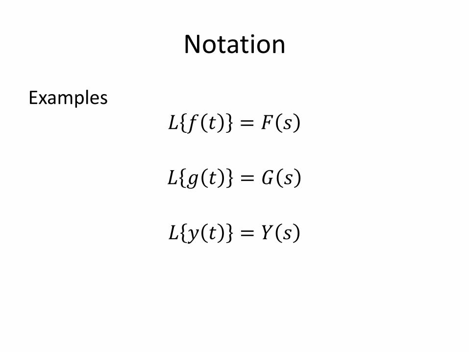
Notation
Examples 𝐿 𝑓 𝑡 = 𝐹 𝑠
𝐿 𝑔 𝑡 = 𝐺 𝑠
𝐿 𝑦 𝑡 = 𝑌 𝑠
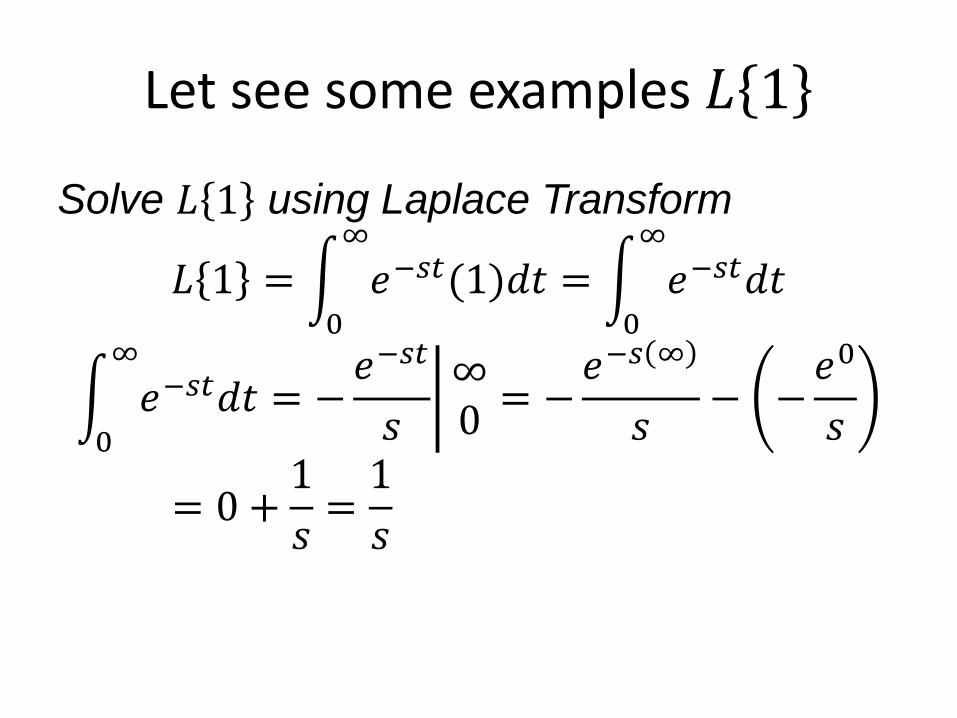
Let see some examples 𝐿 1
Solve 𝐿 1 using Laplace Transform
𝐿 1 = 𝑒−𝑠𝑡(1)𝑑𝑡∞
0
= 𝑒−𝑠𝑡𝑑𝑡∞
0
𝑒−𝑠𝑡𝑑𝑡∞
0
= −𝑒−𝑠𝑡
𝑠 ∞0
= −𝑒−𝑠 ∞
𝑠− −
𝑒0
𝑠
= 0 +1
𝑠=
1
𝑠
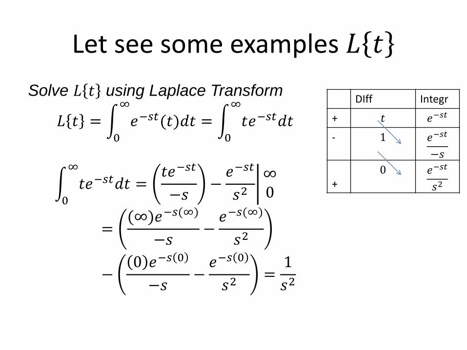
Let see some examples 𝐿 𝑡
Solve 𝐿 𝑡 using Laplace Transform
𝐿 𝑡 = 𝑒−𝑠𝑡(𝑡)𝑑𝑡∞
0
= 𝑡𝑒−𝑠𝑡𝑑𝑡∞
0
𝑡𝑒−𝑠𝑡𝑑𝑡∞
0
=𝑡𝑒−𝑠𝑡
−𝑠−
𝑒−𝑠𝑡
𝑠2 ∞0
=(∞)𝑒−𝑠(∞)
−𝑠−
𝑒−𝑠(∞)
𝑠2
−0 𝑒−𝑠 0
−𝑠−
𝑒−𝑠 0
𝑠2=
1
𝑠2
DIff Integr
+ 𝑡 𝑒−𝑠𝑡
- 1 𝑒−𝑠𝑡
−𝑠
+
0 𝑒−𝑠𝑡
𝑠2
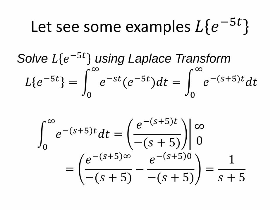
Let see some examples 𝐿 𝑒−5𝑡
Solve 𝐿 𝑒−5𝑡 using Laplace Transform
𝐿 𝑒−5𝑡 = 𝑒−𝑠𝑡(𝑒−5𝑡)𝑑𝑡∞
0
= 𝑒−(𝑠+5)𝑡𝑑𝑡∞
0
𝑒−(𝑠+5)𝑡𝑑𝑡∞
0
=𝑒−(𝑠+5)𝑡
−(𝑠 + 5) ∞0
=𝑒−(𝑠+5)∞
−(𝑠 + 5)−
𝑒− 𝑠+5 0
−(𝑠 + 5)=
1
𝑠 + 5
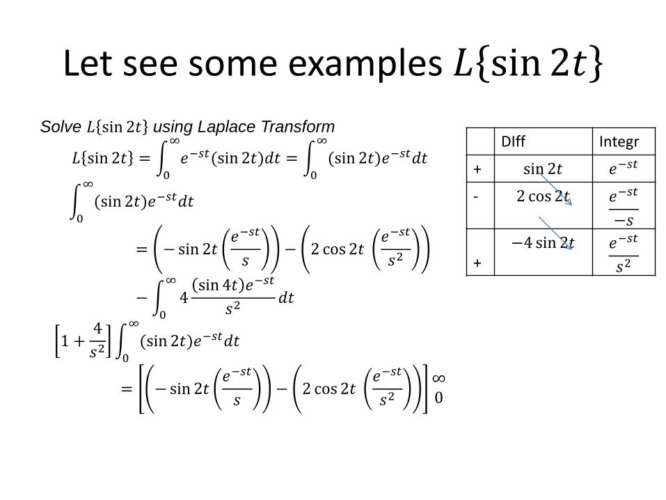
Let see some examples 𝐿 sin 2𝑡
Solve 𝐿 sin 2𝑡 using Laplace Transform
𝐿 sin 2𝑡 = 𝑒−𝑠𝑡(sin 2𝑡)𝑑𝑡∞
0
= (sin 2𝑡)𝑒−𝑠𝑡𝑑𝑡∞
0
(sin 2𝑡)𝑒−𝑠𝑡𝑑𝑡∞
0
= − sin 2𝑡𝑒−𝑠𝑡
𝑠− 2 cos 2𝑡
𝑒−𝑠𝑡
𝑠2
− 4sin 4𝑡 𝑒−𝑠𝑡
𝑠2 𝑑𝑡∞
0
1 +4
𝑠2 (sin 2𝑡)𝑒−𝑠𝑡𝑑𝑡∞
0
= − sin 2𝑡𝑒−𝑠𝑡
𝑠− 2 cos 2𝑡
𝑒−𝑠𝑡
𝑠2
∞0
DIff Integr
+ sin 2𝑡 𝑒−𝑠𝑡
- 2 cos 2𝑡 𝑒−𝑠𝑡
−𝑠
+
−4 sin 2𝑡 𝑒−𝑠𝑡
𝑠2
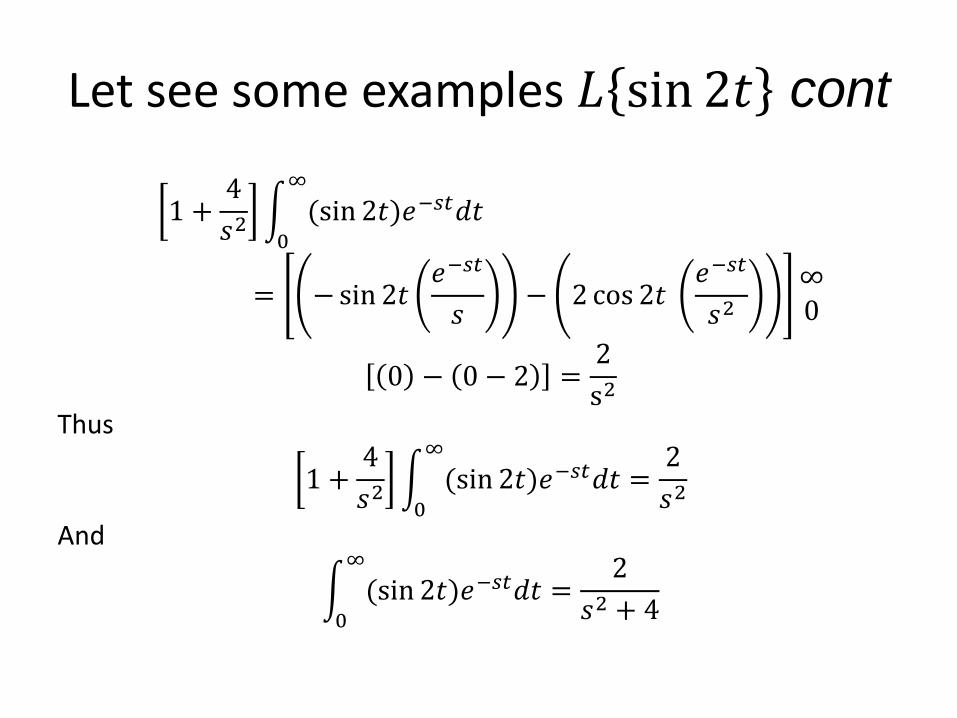
Let see some examples 𝐿 sin 2𝑡 cont
1 +4
𝑠2 (sin 2𝑡)𝑒−𝑠𝑡𝑑𝑡
∞
0
= −sin 2𝑡𝑒−𝑠𝑡
𝑠− 2 cos 2𝑡
𝑒−𝑠𝑡
𝑠2
∞0
0 − 0 − 2 =2
s2
Thus
1 +4
𝑠2 (sin 2𝑡)𝑒−𝑠𝑡𝑑𝑡
∞
0
=2
𝑠2
And
(sin 2𝑡)𝑒−𝑠𝑡𝑑𝑡∞
0
=2
𝑠2 + 4
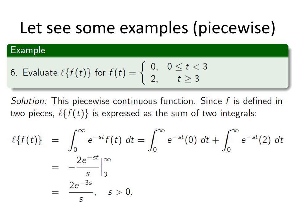
Let see some examples (piecewise)
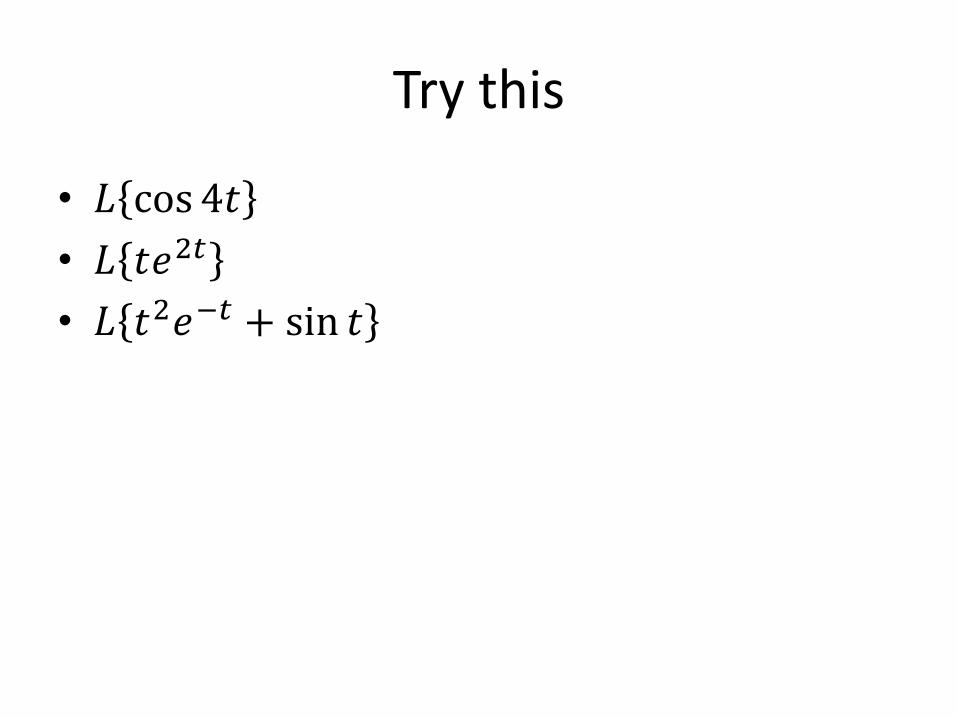
Try this
• 𝐿 cos 4𝑡
• 𝐿 𝑡𝑒2𝑡
• 𝐿 𝑡2𝑒−𝑡 + sin 𝑡
TRANSLATION THEOREM
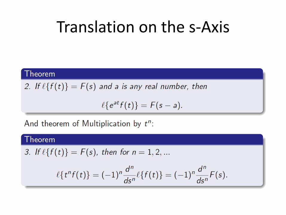
Translation on the s-Axis
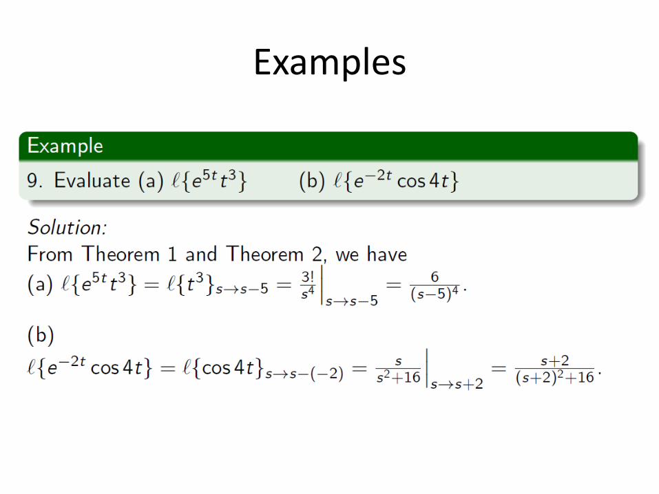
Examples
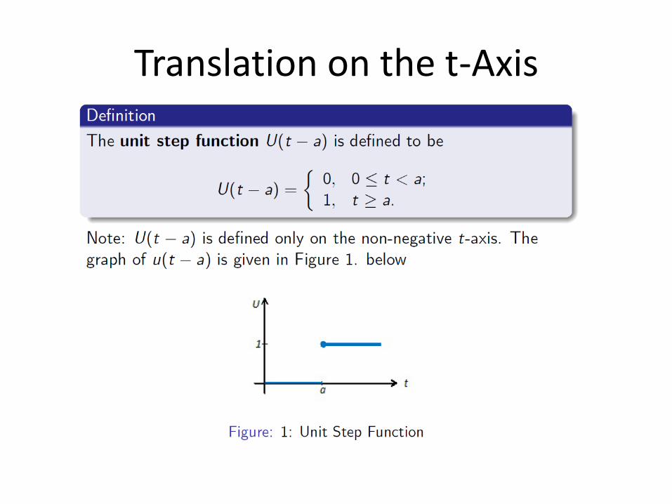
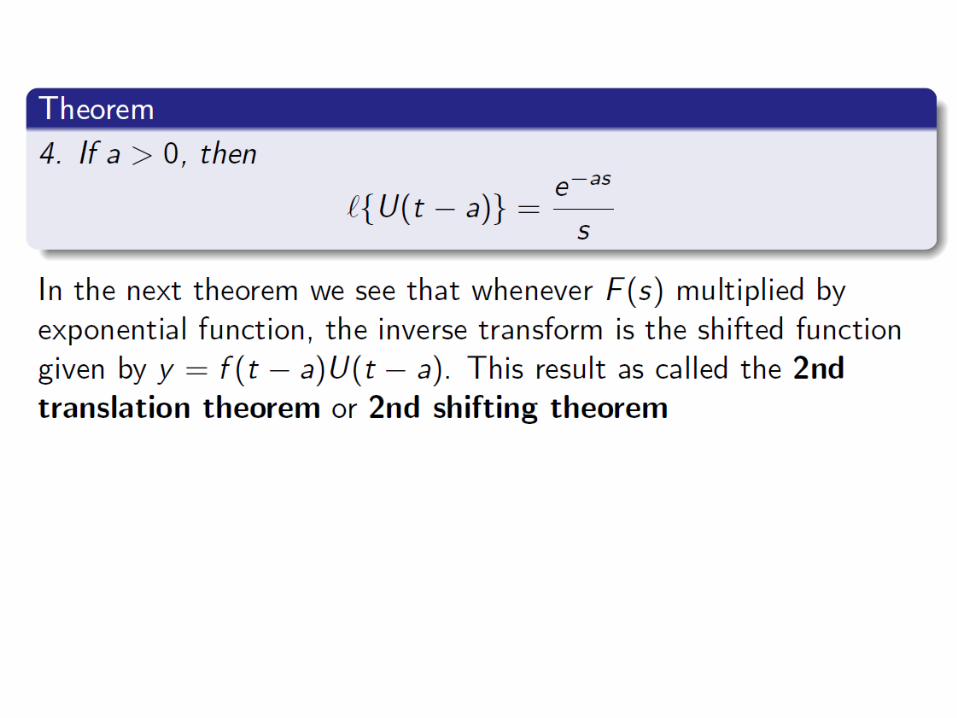
Translation on the t-Axis
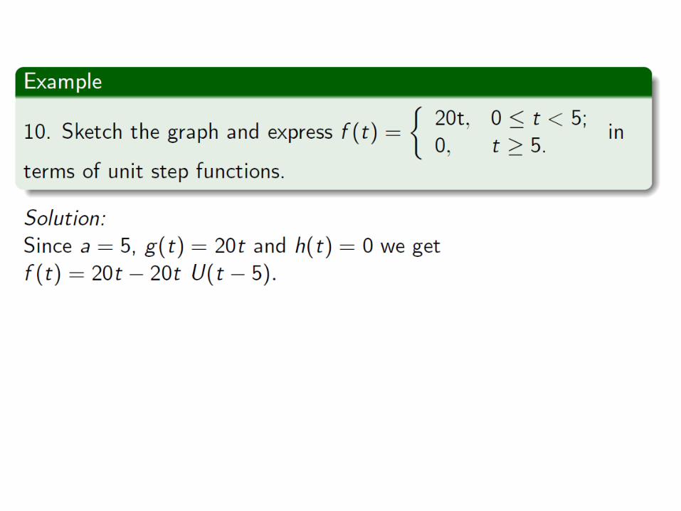
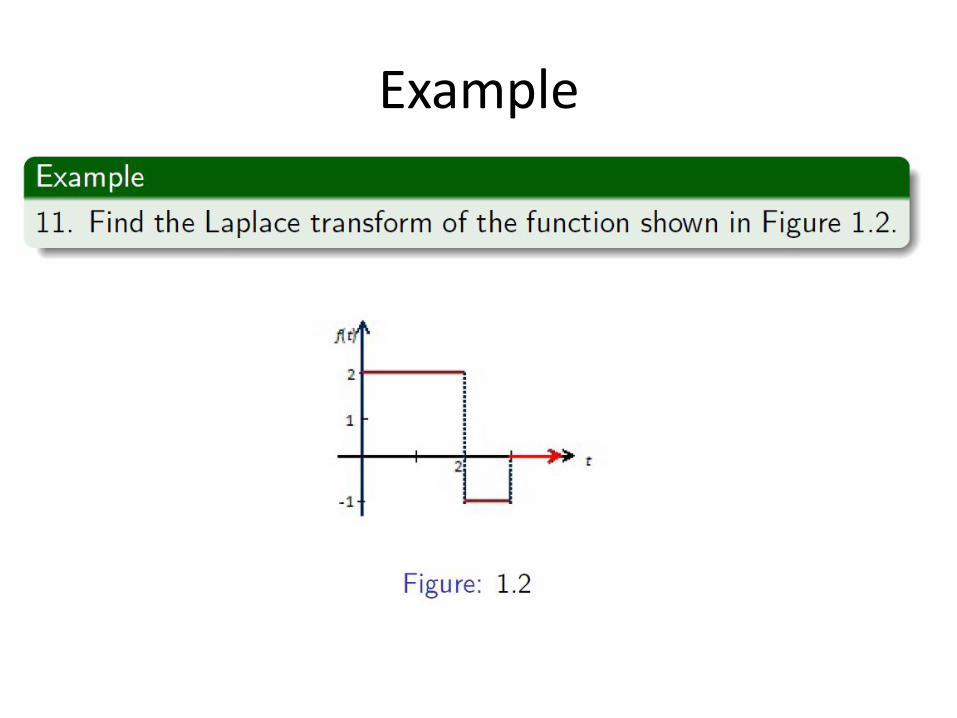
Example
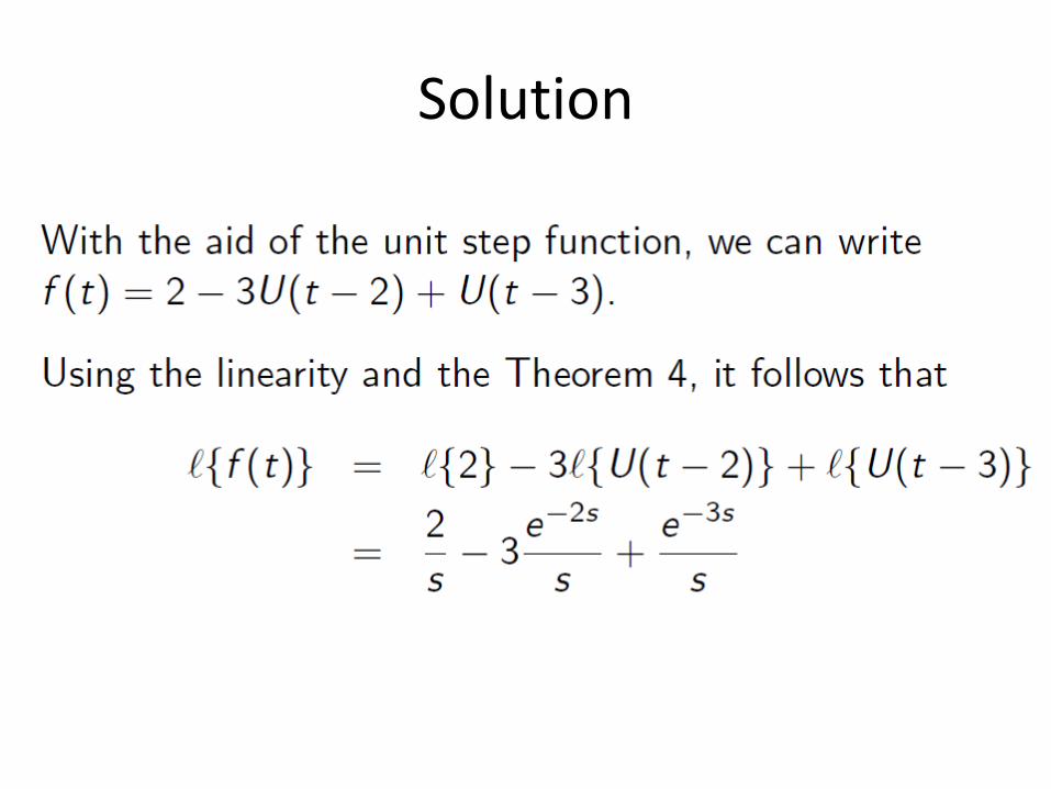
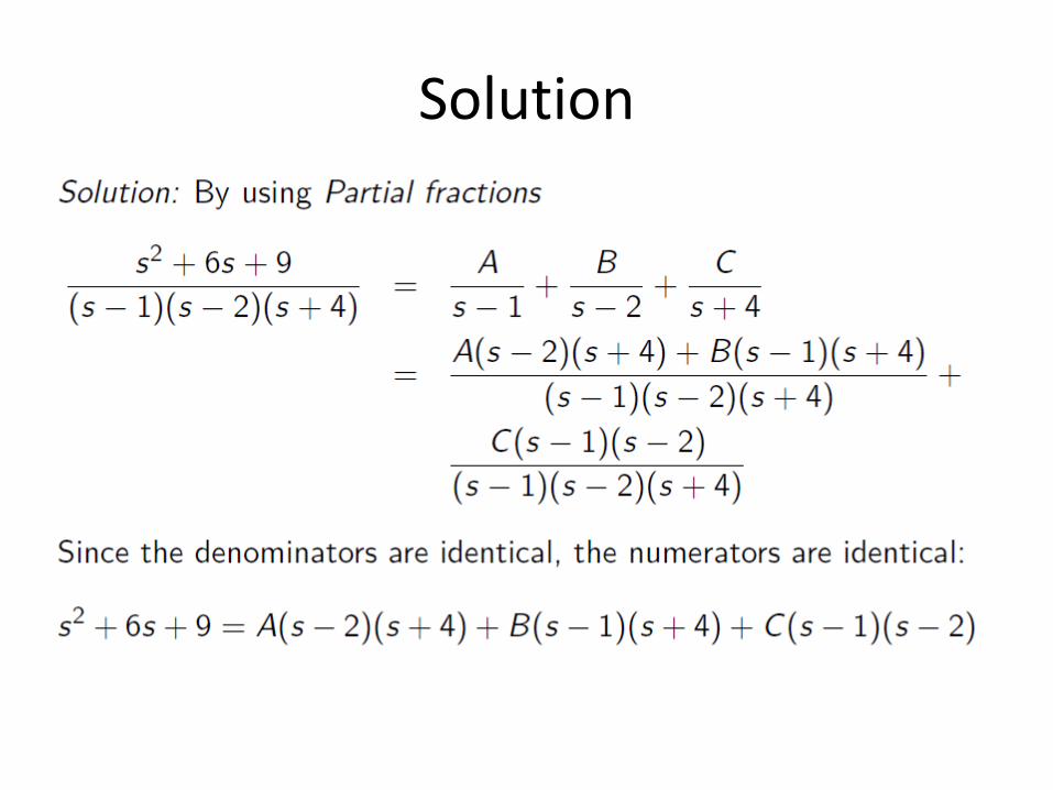
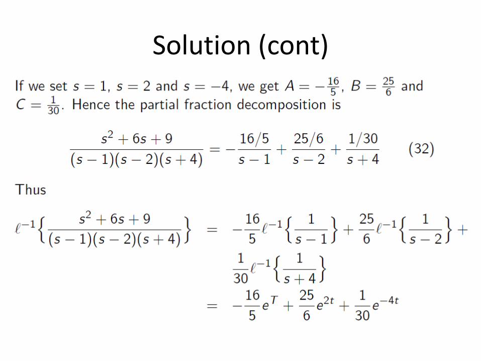
Solution
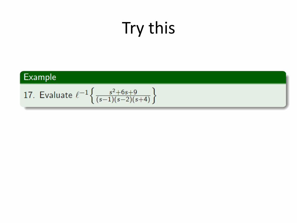
Evaluate
CONVOLUTION AND TRANSFORM OF PERIODIC FUNCTION
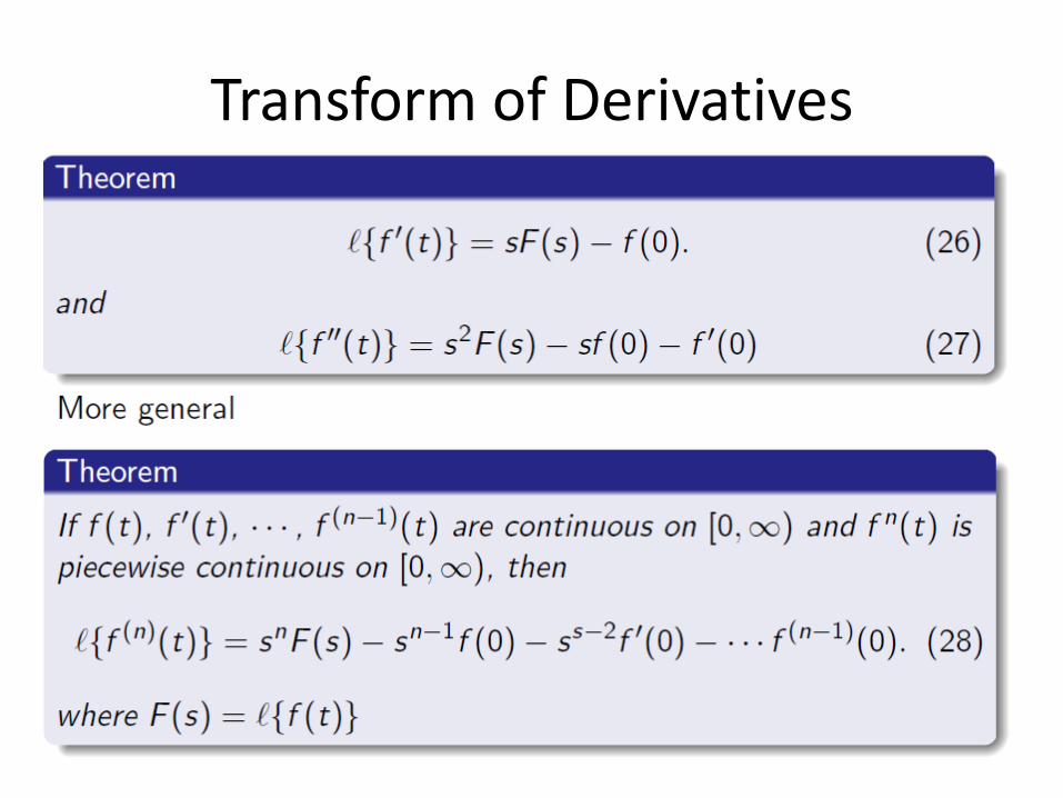
Transform of Derivatives
Transform of Derivatives
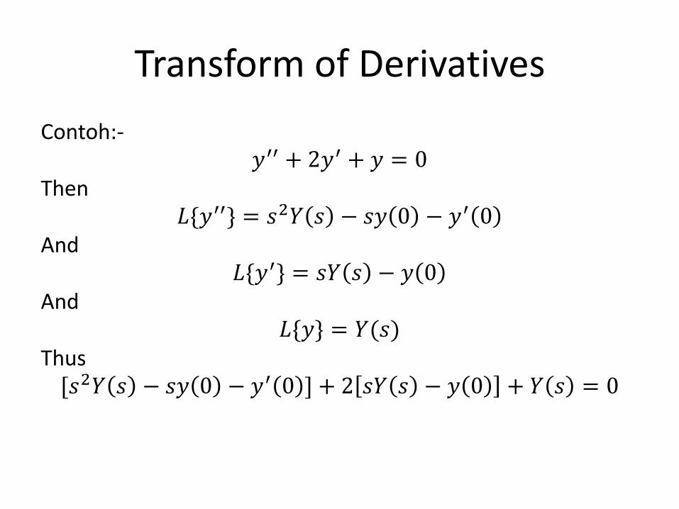
Contoh:- 𝑦′′ + 2𝑦′ + 𝑦 = 0
Then 𝐿*𝑦′′+ = 𝑠2𝑌 𝑠 − 𝑠𝑦 0 − 𝑦′ 0
And 𝐿*𝑦′+ = 𝑠𝑌 𝑠 − 𝑦 0
And 𝐿*𝑦+ = 𝑌(𝑠)
Thus ,𝑠2𝑌 𝑠 − 𝑠𝑦 0 − 𝑦′ 0 - + 2 𝑠𝑌 𝑠 − 𝑦 0 + 𝑌 𝑠 = 0
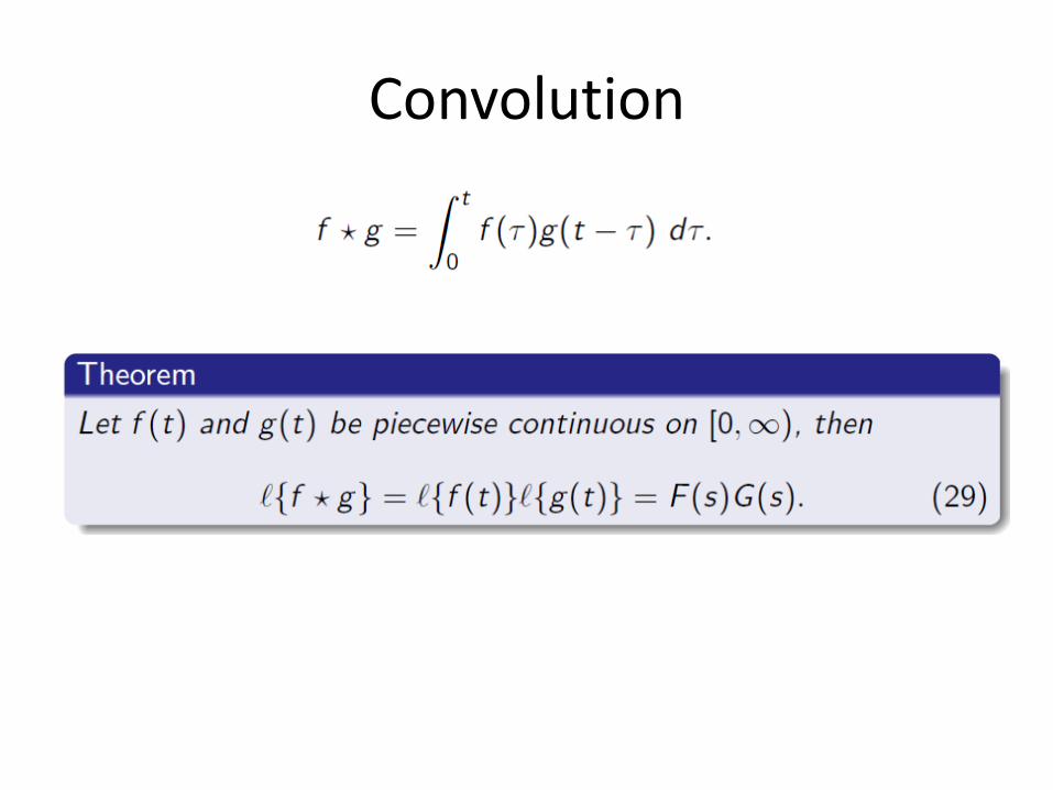
Convolution
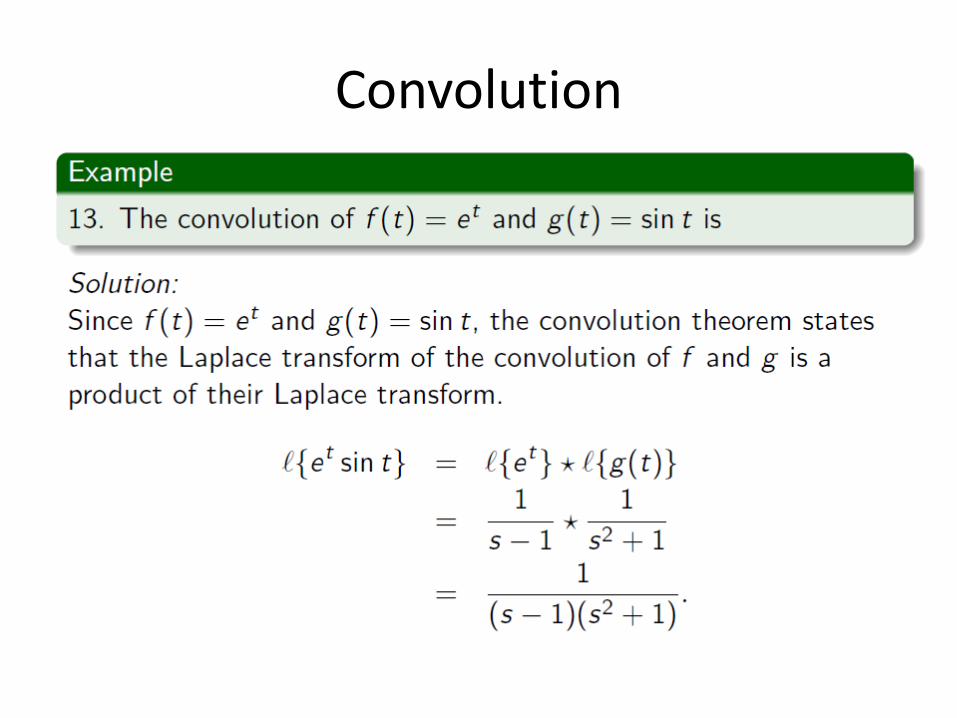
Convolution
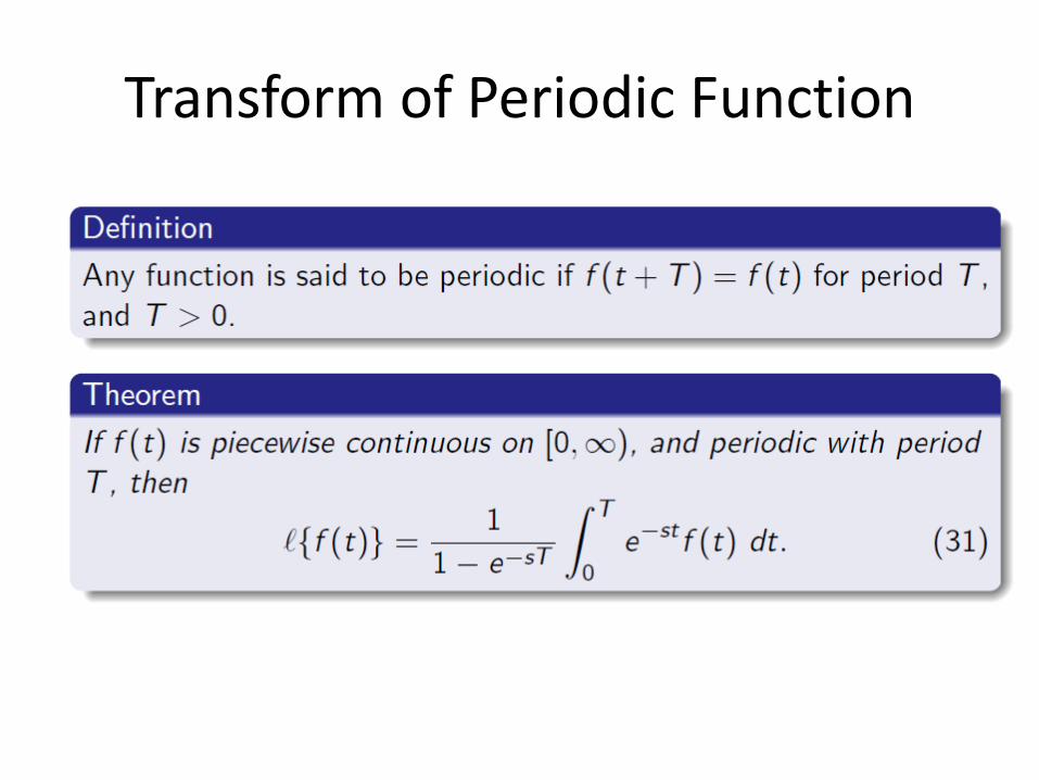
Transform of Periodic Function
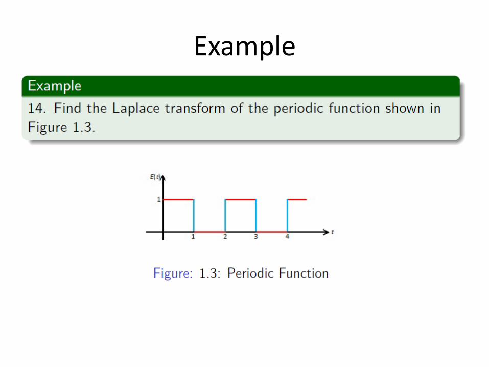
Example
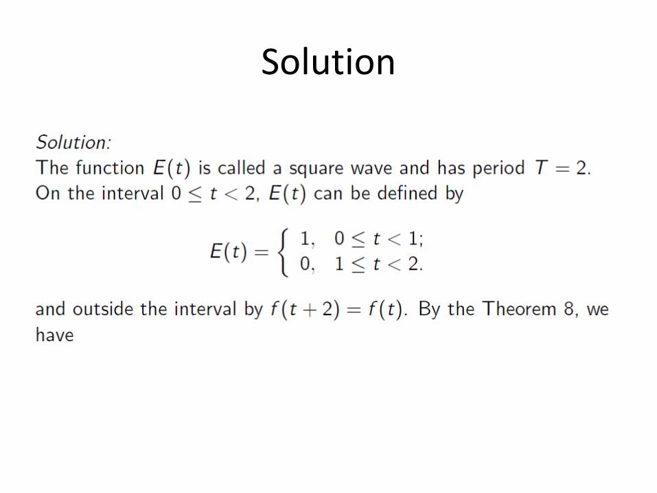
Solution
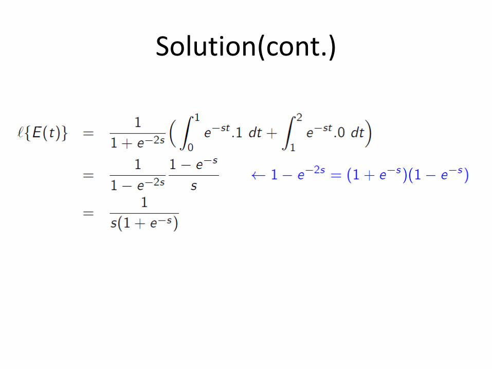
Solution(cont.)
INVERSE LAPLACE TRANSFORM
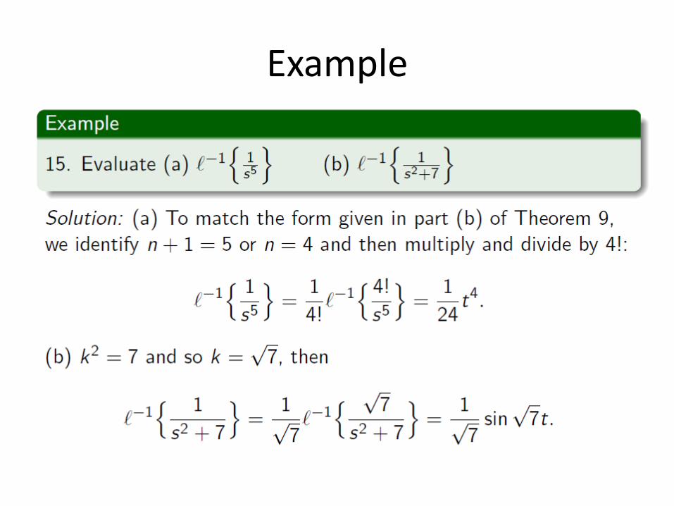
Example
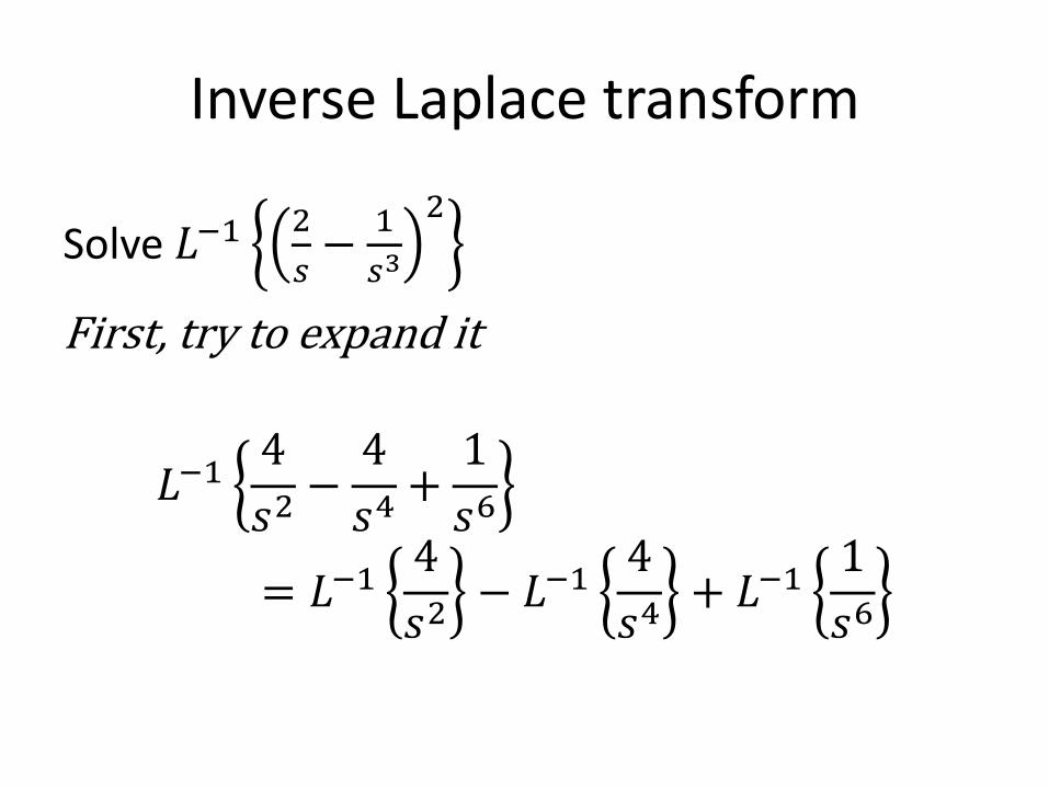
Inverse Laplace transform
Solve 𝐿−1 2
𝑠−
1
𝑠3
2
First, try to expand it
𝐿−14
𝑠2−
4
𝑠4+
1
𝑠6
= 𝐿−14
𝑠2− 𝐿−1
4
𝑠4+ 𝐿−1
1
𝑠6
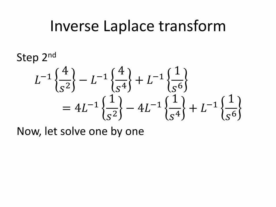
Inverse Laplace transform
Step 2nd
𝐿−14
𝑠2− 𝐿−1
4
𝑠4+ 𝐿−1
1
𝑠6
= 4𝐿−11
𝑠2− 4𝐿−1
1
𝑠4+ 𝐿−1
1
𝑠6
Now, let solve one by one
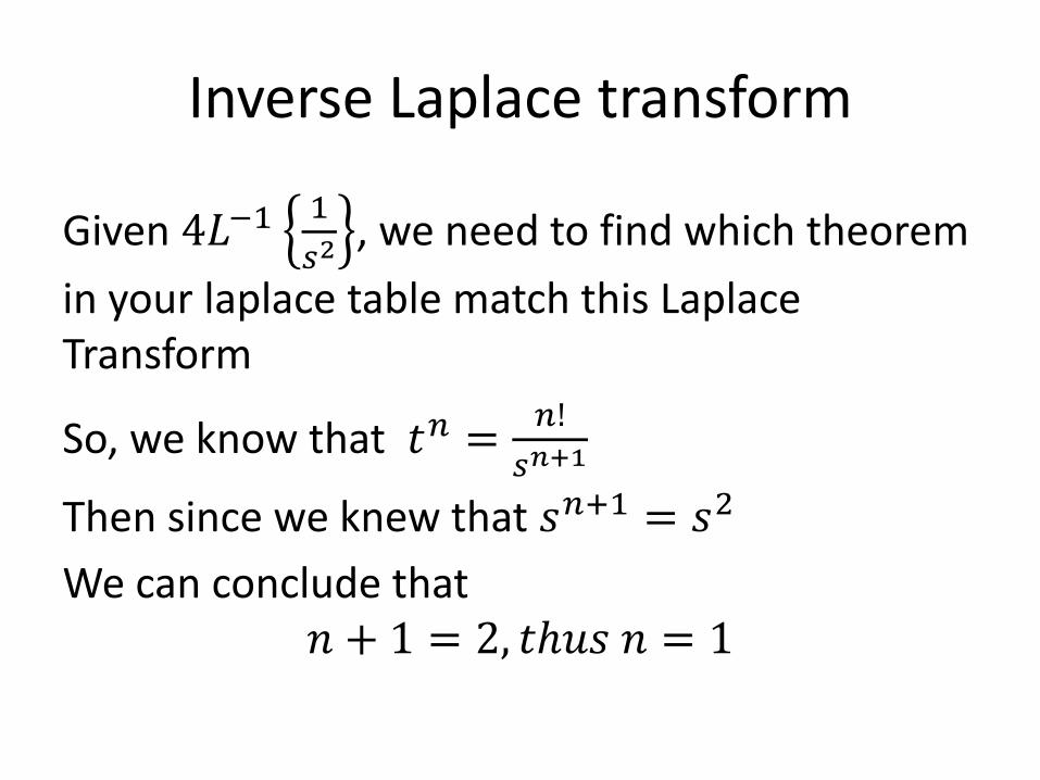
Inverse Laplace transform
Given 4𝐿−1 1
𝑠2 , we need to find which theorem
in your laplace table match this Laplace Transform
So, we know that 𝑡𝑛 =𝑛!
𝑠𝑛+1
Then since we knew that 𝑠𝑛+1 = 𝑠2
We can conclude that 𝑛 + 1 = 2, 𝑡𝑢𝑠 𝑛 = 1
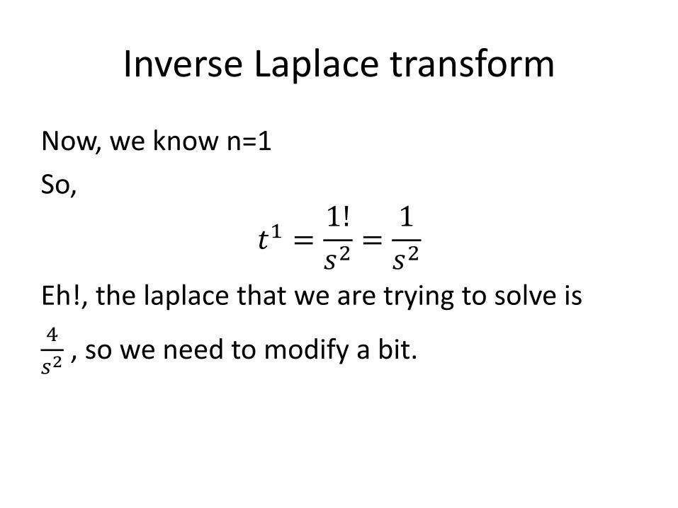
Inverse Laplace transform
Now, we know n=1
So,
𝑡1 =1!
𝑠2=
1
𝑠2
Eh!, the laplace that we are trying to solve is 4
𝑠2 , so we need to modify a bit.
Inverse Laplace transform
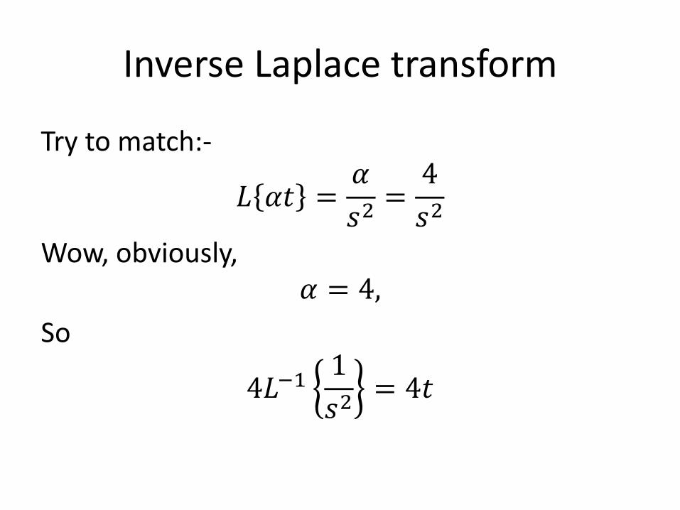
Try to match:-
𝐿 𝛼𝑡 =𝛼
𝑠2=
4
𝑠2
Wow, obviously, 𝛼 = 4,
So
4𝐿−11
𝑠2= 4𝑡
Inverse Laplace transform
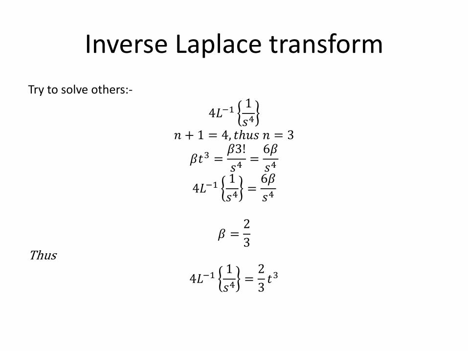
Try to solve others:-
4𝐿−11
𝑠4
𝑛 + 1 = 4, 𝑡𝑢𝑠 𝑛 = 3
𝛽𝑡3 =𝛽3!
𝑠4=
6𝛽
𝑠4
4𝐿−11
𝑠4=
6𝛽
𝑠4
𝛽 =2
3
Thus
4𝐿−11
𝑠4=
2
3𝑡3
Inverse Laplace transform
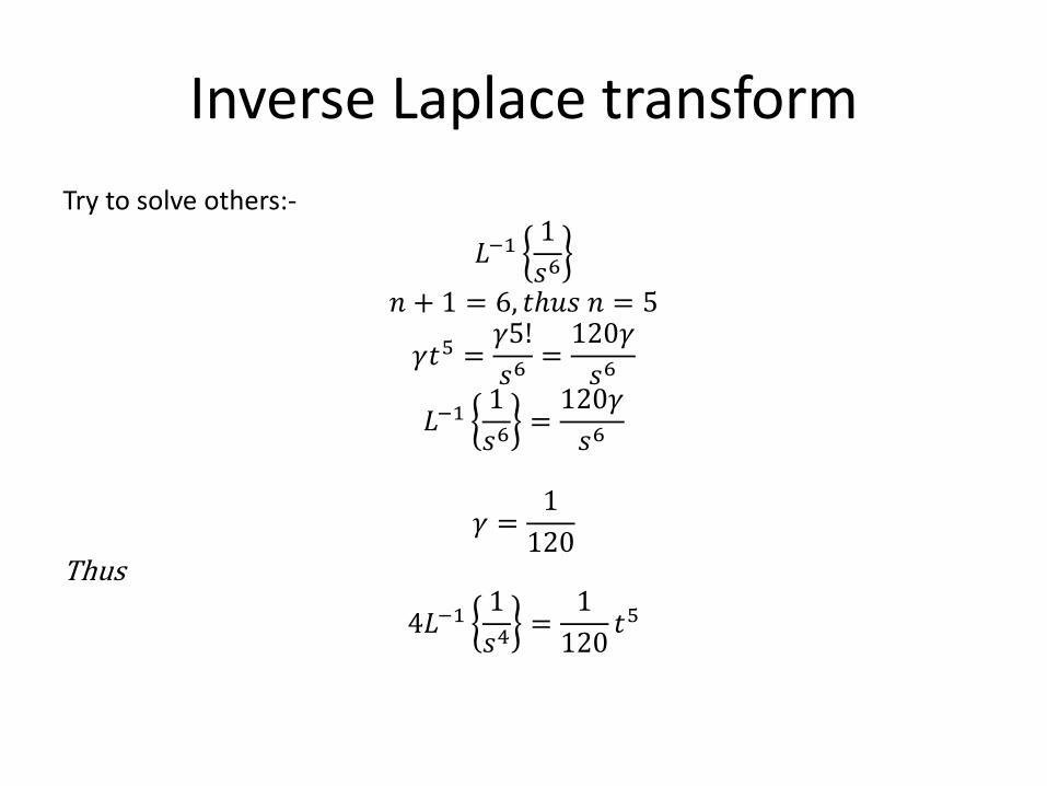
Try to solve others:-
𝐿−11
𝑠6
𝑛 + 1 = 6, 𝑡𝑢𝑠 𝑛 = 5
𝛾𝑡5 =𝛾5!
𝑠6=
120𝛾
𝑠6
𝐿−11
𝑠6=
120𝛾
𝑠6
𝛾 =1
120
Thus
4𝐿−11
𝑠4=
1
120𝑡5
Inverse Laplace transform
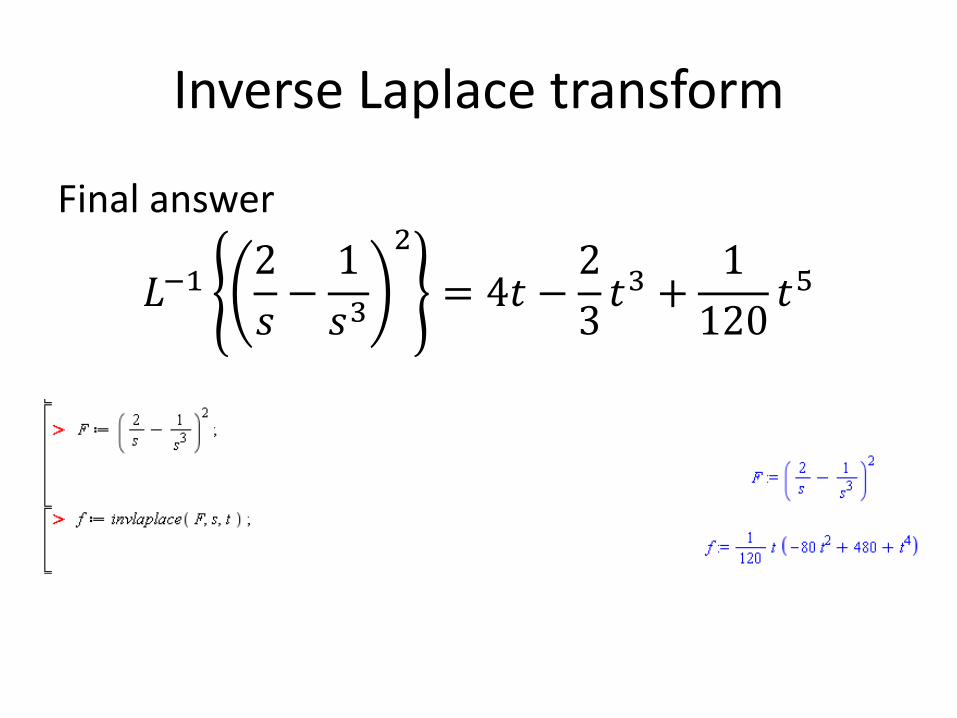
Final answer
𝐿−12
𝑠−
1
𝑠3
2
= 4𝑡 −2
3𝑡3 +
1
120𝑡5
Try this
Solution
Solution (cont)
PROPERTIES OF INVERSE LAPLACE TRANSFORM
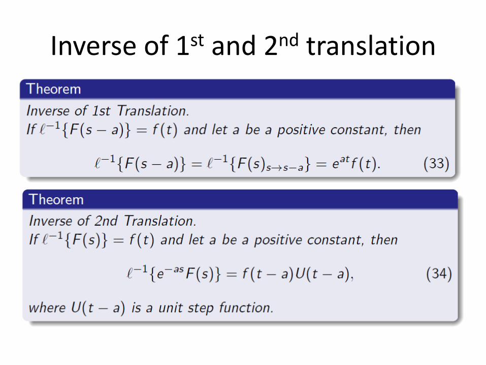
Inverse of 1st and 2nd translation
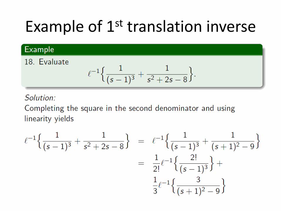
Example of 1st translation inverse
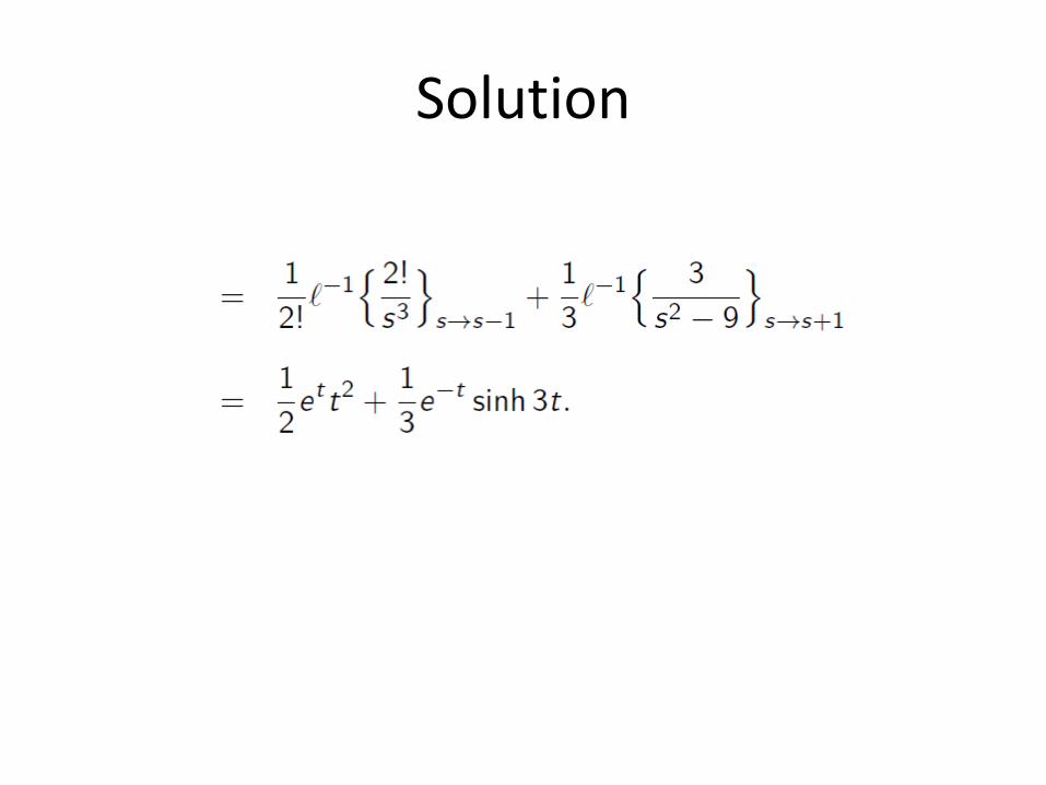
Solution
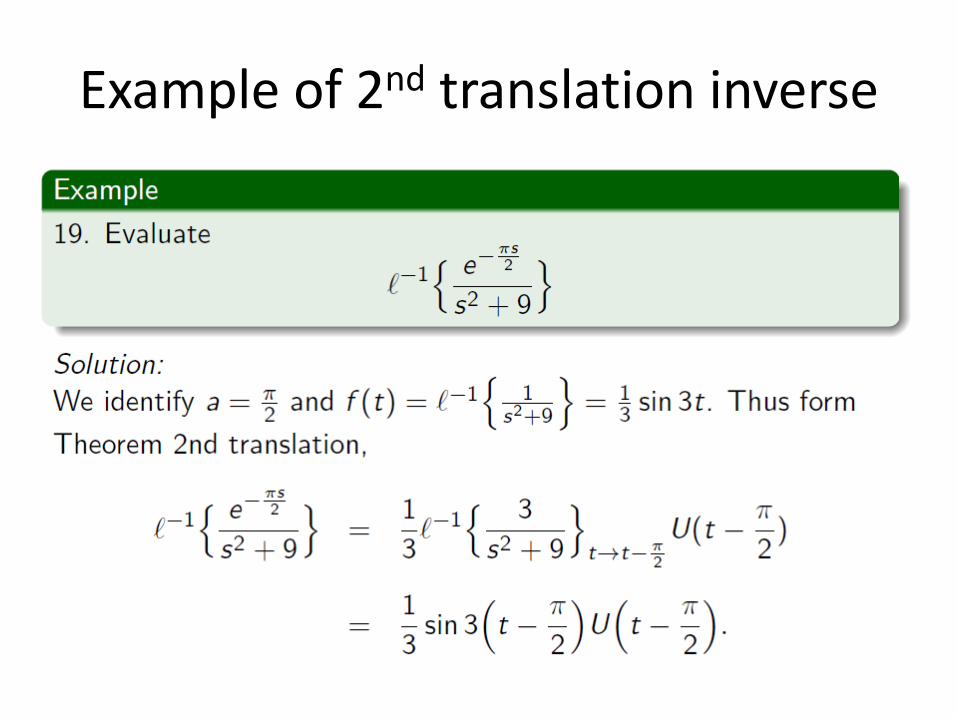
Example of 2nd translation inverse
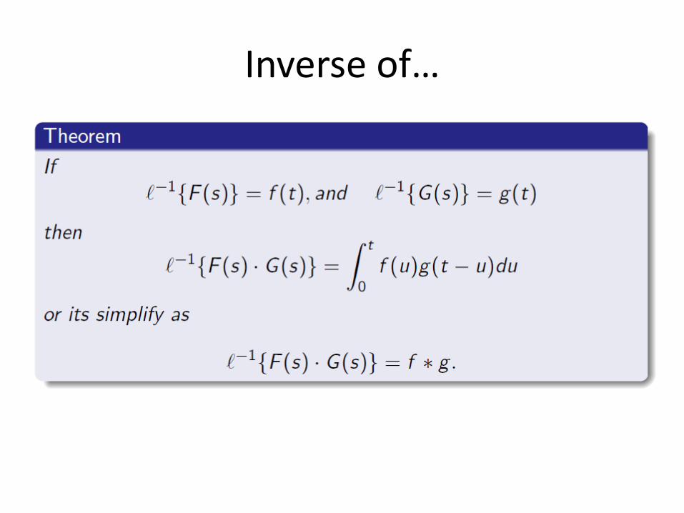
Inverse of…
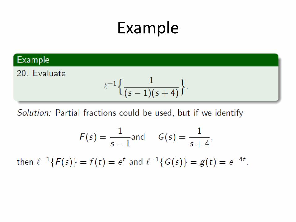
Example
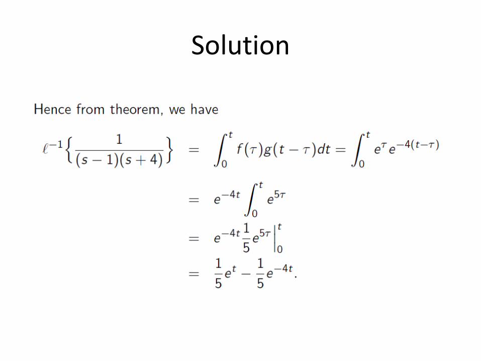
Solution

SOLUTION OF INITIAL VALUE PROBLEM
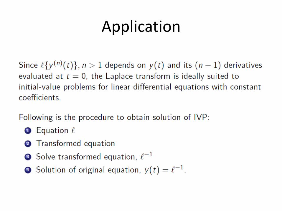
Application
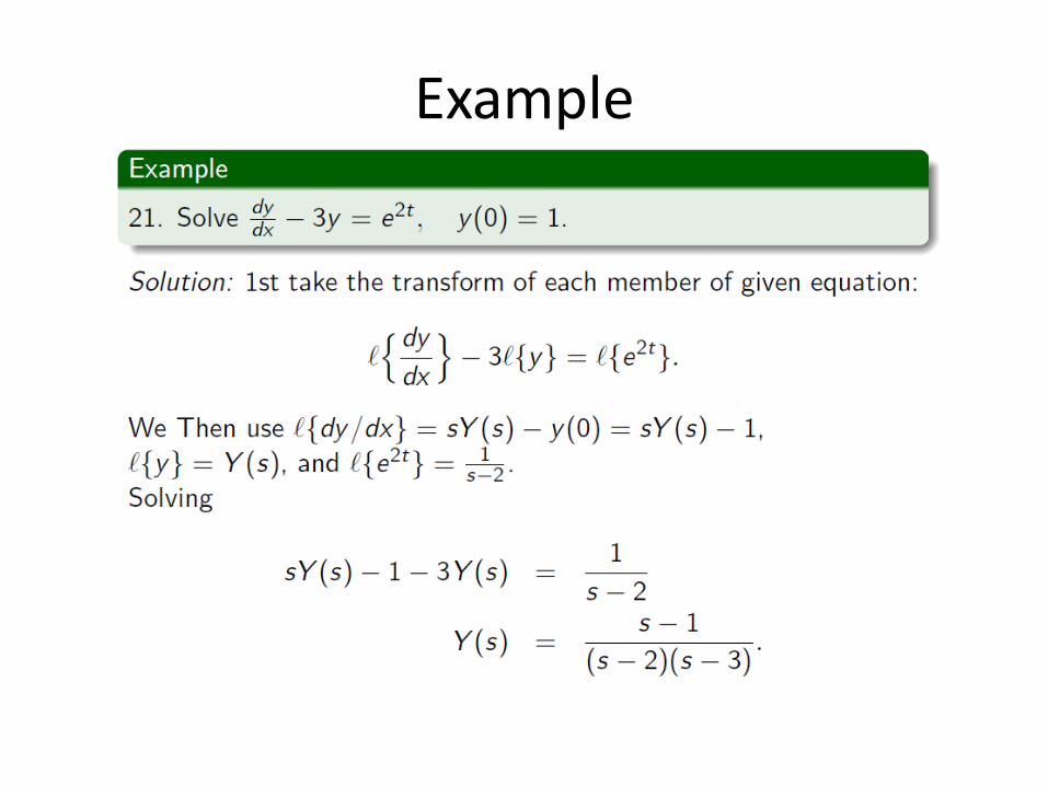
Example
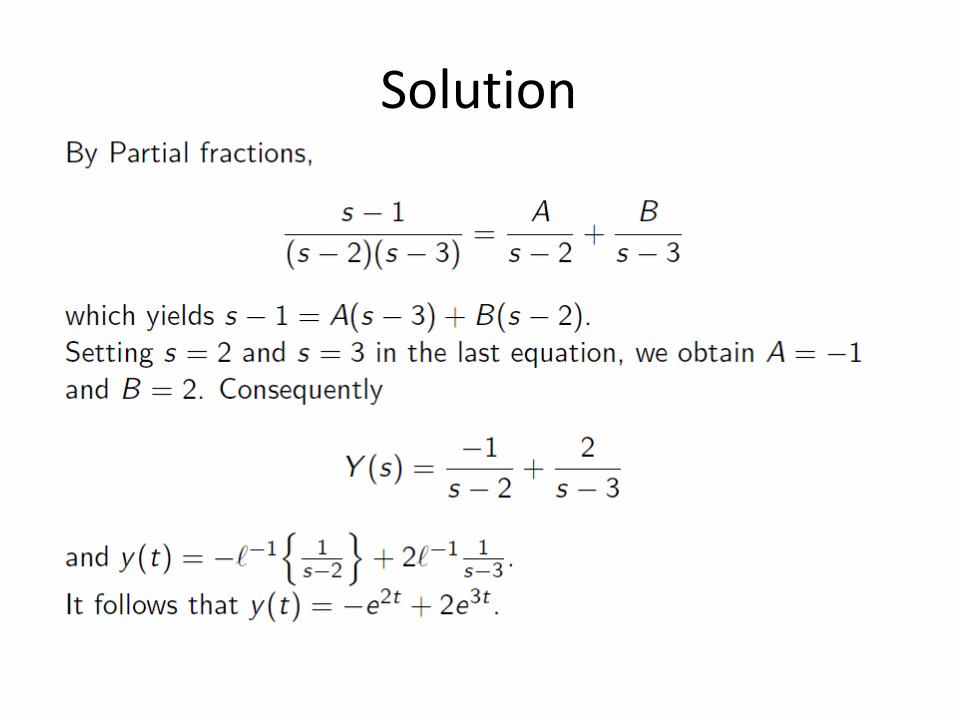
Solution
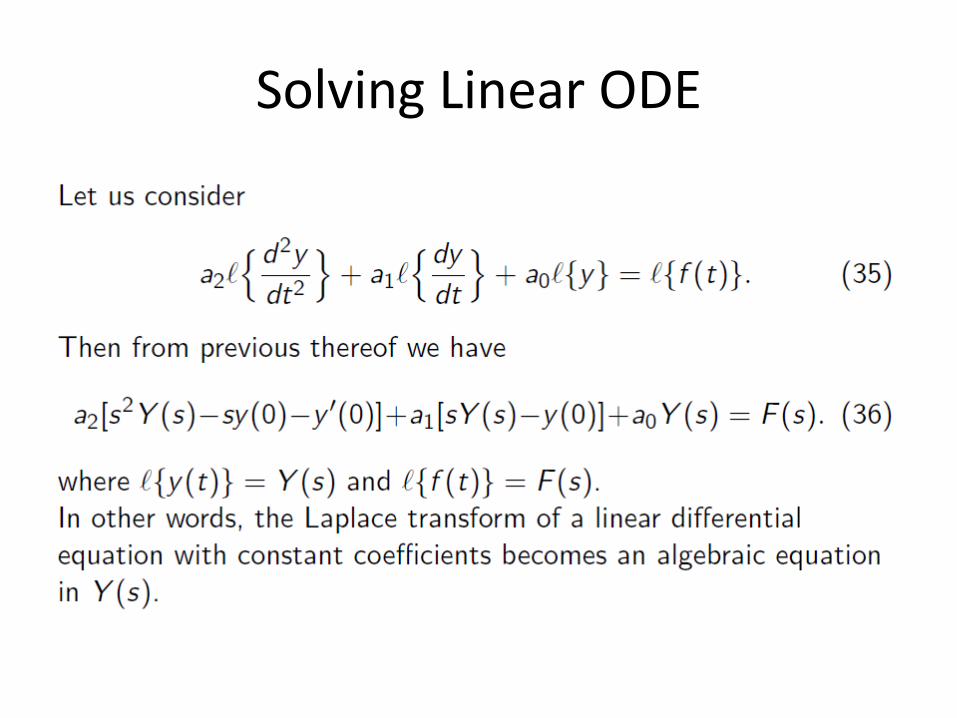
Solving Linear ODE
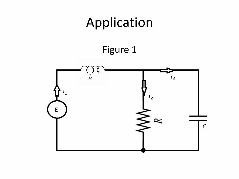
Application
Figure 1
𝑖1
𝑖3
𝑖2
𝐿
𝐶
Application
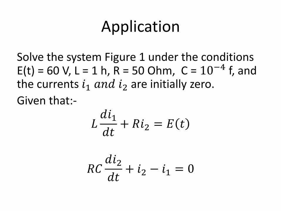
Solve the system Figure 1 under the conditions E(t) = 60 V, L = 1 h, R = 50 Ohm, C = 10−4 f, and the currents 𝑖1 𝑎𝑛𝑑 𝑖2 are initially zero.
Given that:-
𝐿𝑑𝑖1𝑑𝑡
+ 𝑅𝑖2 = 𝐸 𝑡
𝑅𝐶𝑑𝑖2𝑑𝑡
+ 𝑖2 − 𝑖1 = 0
Application
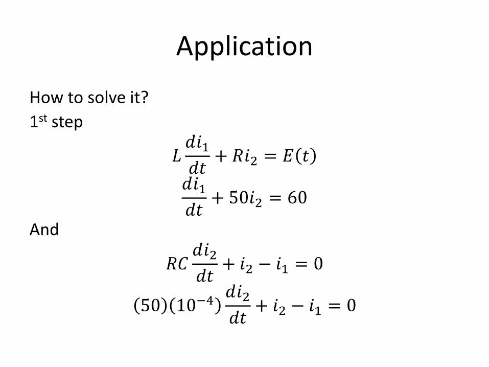
How to solve it?
1st step
𝐿𝑑𝑖1𝑑𝑡
+ 𝑅𝑖2 = 𝐸 𝑡
𝑑𝑖1𝑑𝑡
+ 50𝑖2 = 60
And
𝑅𝐶𝑑𝑖2𝑑𝑡
+ 𝑖2 − 𝑖1 = 0
50 10−4𝑑𝑖2𝑑𝑡
+ 𝑖2 − 𝑖1 = 0
Application
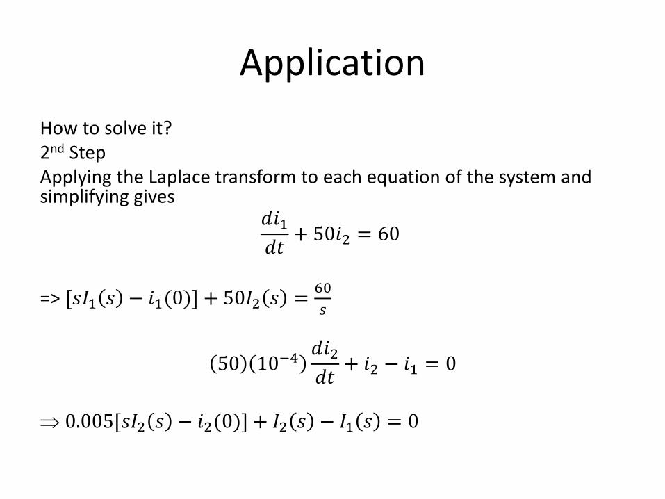
How to solve it? 2nd Step Applying the Laplace transform to each equation of the system and simplifying gives
𝑑𝑖1𝑑𝑡
+ 50𝑖2 = 60
=> ,𝑠𝐼1 𝑠 − 𝑖1(0)- + 50𝐼2 𝑠 =60
𝑠
50 10−4𝑑𝑖2𝑑𝑡
+ 𝑖2 − 𝑖1 = 0
0.005,𝑠𝐼2 𝑠 − 𝑖2(0)- + 𝐼2 𝑠 − 𝐼1 𝑠 = 0
Application
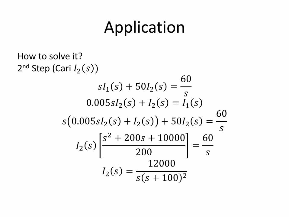
How to solve it? 2nd Step (Cari 𝐼2 𝑠 )
𝑠𝐼1 𝑠 + 50𝐼2 𝑠 =60
𝑠
0.005𝑠𝐼2 𝑠 + 𝐼2 𝑠 = 𝐼1 𝑠
𝑠 0.005𝑠𝐼2 𝑠 + 𝐼2 𝑠 + 50𝐼2 𝑠 =60
𝑠
𝐼2 𝑠𝑠2 + 200𝑠 + 10000
200=
60
𝑠
𝐼2 𝑠 =12000
𝑠 𝑠 + 100 2
Application
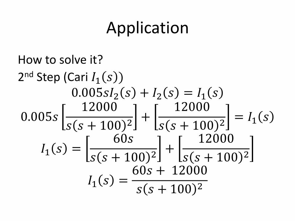
How to solve it?
2nd Step (Cari 𝐼1 𝑠 ) 0.005𝑠𝐼2 𝑠 + 𝐼2 𝑠 = 𝐼1 𝑠
0.005𝑠12000
𝑠 𝑠 + 100 2+
12000
𝑠 𝑠 + 100 2= 𝐼1 𝑠
𝐼1 𝑠 =60𝑠
𝑠 𝑠 + 100 2+
12000
𝑠 𝑠 + 100 2
𝐼1 𝑠 =60𝑠 + 12000
𝑠 𝑠 + 100 2
Application
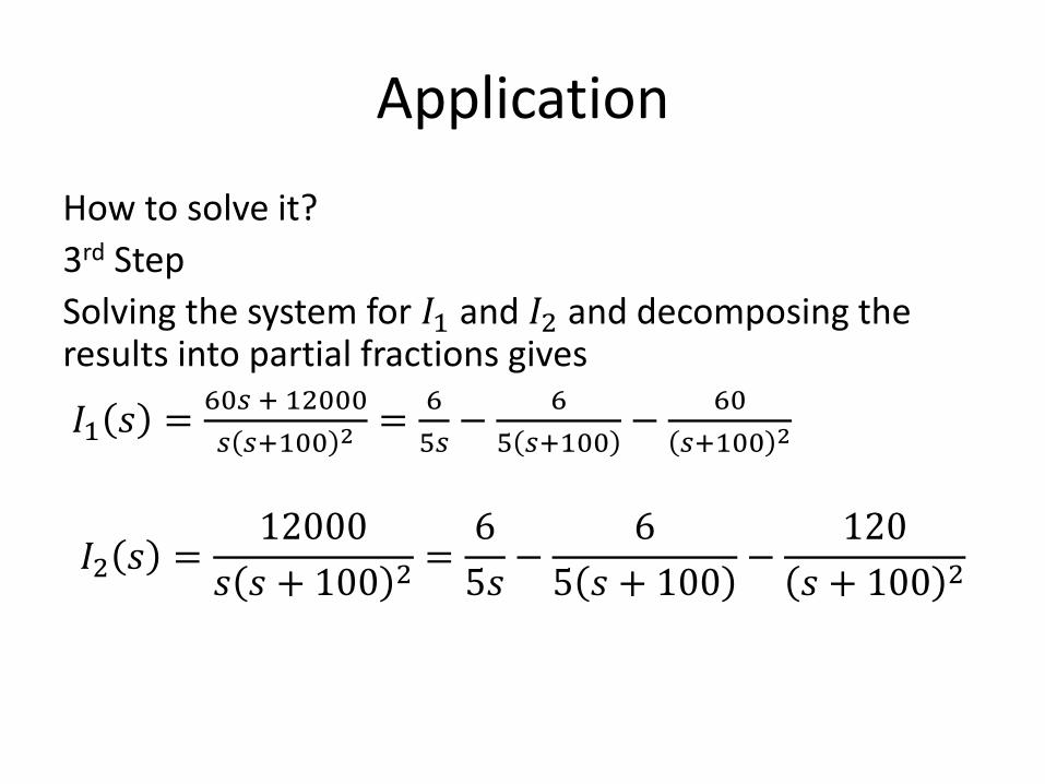
How to solve it?
3rd Step
Solving the system for 𝐼1 and 𝐼2 and decomposing the results into partial fractions gives
𝐼1 𝑠 =60𝑠 + 12000
𝑠 𝑠+100 2 =6
5𝑠−
6
5 𝑠+100−
60
𝑠+100 2
𝐼2 𝑠 =12000
𝑠 𝑠 + 100 2=
6
5𝑠−
6
5 𝑠 + 100−
120
𝑠 + 100 2
Application
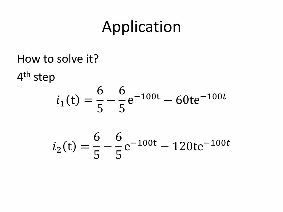
How to solve it?
4th step
𝑖1 t =6
5−
6
5e−100t − 60te−100𝑡
𝑖2 t =6
5−
6
5e−100t − 120te−100𝑡
Top Related