


Languages
Pages
Legal


1
Erasmus University Rotterdam
International Public Management and Policy (IMP) program
Master thesis
The impact of trade expansion on income inequality: analysing the
differences between developed and developing world
Name: Greta Kapustaitė (431481)
1st reader: Prof. Dr. Geske Dijkstra
2nd reader: Prof. Dr. Markus Haverland
Date: 25.07.2016
Word count: 22939

2
Abstract
The relationship between trade liberalization and within-country income inequality has been
observed by a number of researchers, yet in majority of the cases studies have focused on
developed states. Due to the fact that gains associated with trade expansion are not equally
distributed, as more advanced countries are better able to realize trade-related benefits, there are
reasons to expect that trade-inequality effects might differ depending on country’s state of
development. Consequently, this research aims at contributing to the existing pool of literature by
identifying the possible differences in trade impact on within-country income inequality between
developed and developing countries. The data used for the purpose of this analysis covers 91
country during the time period from 1999 to 2008. As the results of panel data regression analysis
reveal, trade expansion leads to higher inequality, yet an interaction term between trade volumes
and variable representing state of development is not significant. Therefore it can be stated that no
differences in trade-inequality effects between countries in different stage of development were
observed.
Key words: trade, within-country income inequality, income distribution, developing world,
developed world.

3
Acknowledgment
During the process of writing this thesis, a number of people have helped me and supported me.
First of all I would like to thank my supervisor, professor Geske Dijkstra, whose guidance,
comments and advices from the very beginning were essential and really helped me to move
forward with this research. I also want to say thank you to my second reader, professor Markus
Haverland, for his comments and recommendations that helped me to improve this thesis. Finally
I would like to thank all the members of my thesis circle: Auste Linkeviciute, Nazli Gulijeva, Joost
van Damme and Ludo Bolling. Their comments and ideas at the initial stages of thesis writing
process made me think about my topic from different perspectives which in turn was really helpful
when formulating the central goal of this research.

4
Table of Contents 1. Introduction ............................................................................................................................................ 6
1.1 Aim of the thesis ............................................................................................................................... 8
1.2 Problem statement ............................................................................................................................. 8
1.3 Sub-questions .................................................................................................................................... 9
1.4 Research approach ............................................................................................................................ 9
1.5 Academic relevance .......................................................................................................................... 9
1.6 Policy relevance ................................................................................................................................ 9
1.7 Outline ............................................................................................................................................ 11
2. Literature review and theoretical framework ........................................................................................ 13
2.1 Theoretical explanations of trade-inequality effects ........................................................................ 13
2.2. Evidence ........................................................................................................................................ 18
2.3 Contributory and explanatory factors .............................................................................................. 27
2.4 Summarizing table .......................................................................................................................... 30
2.5 Theoretical expectations ................................................................................................................. 33
3. Research design .................................................................................................................................... 36
3.1 Empirical methods .......................................................................................................................... 36
3.2 Operationalization ........................................................................................................................... 39
3.3 Country sample ............................................................................................................................... 46
3.4 Reliability and validity .................................................................................................................... 47
4. Empirical analysis ................................................................................................................................. 49
4.1 Descriptive statistics ....................................................................................................................... 49
4.2 Testing the assumptions of multivariate regression analysis ........................................................... 51
4.3 Model selection ............................................................................................................................... 59
4.4 The results ....................................................................................................................................... 60
5. Interpretations and conclusions ............................................................................................................. 65
5.1 Interpretation of the results ............................................................................................................. 65
5.2 Policy recommendations ................................................................................................................. 68
5.3 Limitations ...................................................................................................................................... 69
5.4 Implications for future research ...................................................................................................... 70
5.5 Conclusions ..................................................................................................................................... 70
References ................................................................................................................................................ 72
Appendices ............................................................................................................................................... 77

5
List of tables:
Table 1. Summarizing table ...................................................................................................................... 31
Table 2. Summary statistics ...................................................................................................................... 50
Table 3. Results of the normality tests ...................................................................................................... 53
Table 4. Results of the normality tests ...................................................................................................... 55
Table 5. Correlation matrix ....................................................................................................................... 58
Table 6. Test for presence of heteroscedasticity........................................................................................ 59
Table 7. WLS model table ........................................................................................................................ 62
Table 8. WLS modified model table (robustness test) .............................................................................. 63
List of figures:
Figure 1. Developing countries ................................................................................................................. 34
Figure 2. Developed countries .................................................................................................................. 35
List of graphs:
Graph 1. Frequency distribution histogram for GINI ................................................................................ 52
Graph 2. Frequency distribution histogram for transformed GINI ............................................................ 52
Graph 3.Frequency distribution histogram for trade-to-GDP .................................................................... 54
Graph 4. Frequency distribution histogram for transformed trade-to-GDP ............................................... 54
Graph 5. Scatter plot for linearity ............................................................................................................. 57
List of appendices:
Appendix 1. Country sample .................................................................................................................... 77
Appendix 2. Country division based on the World Bank’s country classification .................................... 78
Appendix 3. Normality tests ..................................................................................................................... 79
Appendix 4. Summary of transformations for normality .......................................................................... 83
Appendix 5. Scatter plots for linearity ...................................................................................................... 84
Appendix 6. Full model tables .................................................................................................................. 85
Appendix 7. Robustness check ................................................................................................................. 86

6
1. Introduction
Over the years the vast majority of countries all around the world have witnessed a tremendous
growth in levels of income inequality. According to OECD reports, the difference between
earnings of the richest and the poorest 10% of the population has increased from seven to ten times
in most OECD countries since 1980s, and hence the current income gap is the highest in more than
three decades. In addition to that, a similar trend has been observed in majority of developing
countries (including emerging economies like China, or India) where the difference between the
income of rich and poor is said to be five times larger than in developed countries (OECD, 2015).
However, it is important to note that such figures reveal only half of the story, as in academic
literature, generally three types of income inequality are distinguished: the global inequality
(focusing on world income distribution), between–country inequality (based on population
weighted mean income) and within-country inequality (reflecting uneven income distribution on
a country level) (Milanovic, 2006; Sala-i-Martin, 2002). Looking from the global perspective,
findings about the direction of change in global income gap are quite diverse, whereas regarding
within-country inequality, the trends are more evident and show growing income gap (Ghose,
2001; Liberati, 2015). Although it has been widely acknowledged that certain level of inequality
will always exist, reducing it and achieving more egalitarian income distribution within the country
remains important due to the negative effects associated with high income gap. These effects are
numerous: inequality threatens country’s political stability by dividing the society, limits the
potential for economic growth, development, and weakens the effects of growth on poverty
reduction (The World Bank, 2007; Jaumotte, Lall, & Papageorgiou, 2013).
In academic literature the issue of inequality has been widely addressed focusing on the potential
triggers and one of the common findings of such studies is the effect of economic globalization.
More specifically, it has been found that in the context of growingly integrated and interrelated
global economy, trade related factors (trade volumes, openness, liberalization, policies) have an
impact on economic growth and thus on income levels and changes in inequality levels (Ghose,
2001; Bergh & Nilsson, 2010; Keeley, 2015). In addition, it has been argued that trade
liberalization by nature means modifications, thus distributional changes are very likely to occur
(Winters, McCulloch, & McKay, 2004). This implies that the more countries are engaged in trade,
the bigger the changes in levels of income inequality could get. Since economists agree that high
7
income inequality is harmful for the economy, the trade-inequality relationship should receive
significantly more attention with the majority of countries all around the globe becoming more
and more engaged in international trade.
Trade expansion is often associated with significant gains for countries involved in trade-
relationship with other parties. It has been argued that more trade will increase national welfare,
bring more prosperity and development (Bliss, 2007). However, trade-related benefits are not
distributed equally across countries. Since richer states have more financial capabilities and are
able to better use the opportunities provided by increasingly globalized economy, benefits from
international trade are likely to be high. Whereas in case of poor, underdeveloped countries that
lack the needed resources, the benefits of trade expansion might be realized at considerable costs,
such as more unequal income distribution. Therefore, considering that in the context of rising
international trade volumes some countries gain more than others, the same could be expected in
terms of trade-inequality relationship.
As the theoretical implications of Heckscher-Ohlin model suggest, more trade should lead to
higher income inequality in developed countries and lower in developing countries. However, the
existent empirical evidence shows that the actual trade impact on income inequality in most of the
cases is inconsistent with the prediction of the standard trade theories. As a matter of fact, lower-
income countries are said to be more vulnerable to the effects of trade liberalization and the trade-
inequality linkages seem to be more pronounced as compared to rich countries (Barro, 2000;
Ravallion, 2001). This implies that further research on trade-inequality relationship is needed,
particularly looking at possible differences in trade effects on different sets of countries, as well as
analysing which countries are better able to realize the gains associated with trade expansion and
in what instances such benefits come at a higher cost of widening income gap. Understanding the
trade-inequality effects is especially important regarding the developing countries which over the
past few decades have been actively seeking to become more involved in international trade.
Consequently, the focal point of this thesis is trade impact on within-country income inequality
and the potential differences in the effects for developed and developing countries
In the following parts of this chapter the aims of the research are presented and a more detailed
problem statement is provided. Afterwards, with the formulated central research question and sub-

8
questions, the relevance of the topic is further explained. Finally the reader is briefly introduced to
the research approach and the outline of the consequent parts of the paper.
1.1 Aim of the thesis
In general terms this thesis aims at contributing to the existing pool of literature on trade and
inequality by analysing the effect of an increase (decrease) in trade on levels of income inequality
in both developing and developed countries. The central goal is to examine whether these effects
differ depending on the level of development and identifying additional factors that might help to
explicate such differences. Hence, this thesis aims to dig deeper into the dynamics of trade-
inequality relationship and expand the existing knowledge with the analysis of more recent data.
Are developing countries more vulnerable to the negative effects associated with trade? Can the
same trends be observed for all countries on the same level of development? What are contributing
factors that could help to explain the differences (if any)? All these questions will be addressed in
the following parts of the research while answering the research question which is presented in the
next part of this chapter.
1.2 Problem statement
Although in the empirical literature the most common findings suggest that trade leads to increase
in inequality, in general studies focusing on this relationship provide quite divergent results and
there are several reasons for that. First of all, as mentioned in the previous part, the outcomes might
vary depending on inequality definition applied. Within-country inequality is said to be more
observable and important from policy and societal perspectives (Cornia, 2003). In addition, there
exists multiple ways to define and measure trade: linkages between trade and inequality have been
studied from the trade policy perspective (analysing the effect of reduction of tariff and non-tariff
barriers) and from the policy outcomes (trade expansion) perspective. Finally, another reason
leading to significantly divergent results might be related to the choice and categorization of
sample countries (Milanovic & Squire, 2005). As a result, different combinations of commonly
used variables produce mixed evidence, which then makes it rather unclear what the real trade-
inequality effect is in different countries. Thus it is clear that due to lack of consensus on trade-
inequality effects, a further research is needed. Consequently, taking into account issues briefly
discussed in this section and recalling the previously presented aims of this research, the following
research question is formulated:

9
What is the difference in trade effects on inequality for developing and developed countries?
1.3 Sub-questions
In order to answer the central research question the following sub-questions will have to be
answered:
1. What are the theories and evidence presented in the literature on the effects of trade on
income inequality in developing and developed countries?
2. How can the variables be operationalized and how can trade-inequality effects be
researched?
3. What are the results of the analysis?
1.4 Academic relevance
The research question that this thesis aims to answer is academically relevant. Using the existent
evidence of trade effect on inequality it encourages to proceed a step forward and to examine
whether trade impact differs depending on level of country development, as more detailed
explanations, or comparisons regarding the differences and similarities in trade-inequality
relationship between developed and developing world are currently lacking. Additionally, the
research question is academically relevant, because it looks at changes in income distribution at
individual country level (within-country income inequality), instead of focusing on global income
inequality which up until now has been a more common choice. Furthermore, the question does
not mainly focus on rich and developed countries, as has been done in the majority of studies on
trade-inequality effects, but also aims to include large number of developing countries and calls
for country distinction. Considering that the importance of distinguishing (categorizing) countries
based on levels of income, or development has already been emphasized in several previously
conducted studies (Barro, 2000; Ravallion, 2001) and based on the fact that such categorization is
even present in theoretical predictions (e.g. the H-O model), it can be stated that country distinction
might actually be crucial for the results. Therefore, answering the presented research question
would certainly contribute to the currently existing pool of knowledge.

10
1.5 Policy relevance
The formulated question is policy relevant as answering it would increase the current
understanding of trade impact on income distribution which is crucial for devising policy measures
aimed at reducing inequality. In addition, given that widening gap between rich and poor raises
social and welfare concerns, defining the differences between trade-inequality effects in developed
and developing countries would allow the more vulnerable states to take stronger measures and
learn from good examples of countries that were able to better mitigate these negative effects. Due
to the fact that high inequality obstructs economic growth potential, the research question is also
relevant from the economic policy perspective. Knowing whether trade impact on income
inequality depends on country’s development level would be useful for creating policies aimed at
helping the more vulnerable countries to better realize the benefits and economic opportunities
provided by trade expansion without having to face the high costs associated with rising inequality
(slower economic growth, higher poverty, etc.).
1.6 Research approach
The presented sub-questions will be answered in separate chapters. To answer the first sub-
question, firstly the theories analysing the relationship between trade and income inequality will
be presented, together with the main theoretical assumptions regarding the trade-inequality effects
in developed and developing countries. Afterwards, different strands of literature on trade-
inequality impact will be reviewed and the main findings and empirical evidence will be discussed.
Finally, based on the literature review and theory, the theoretical framework will be built together
with theoretical expectations of this research. The second sub-question will be answered by
presenting the research design and justification for the choice of the design. In addition to that,
data that is going to be used for the actual analysis will be presented, including the description of
the variables. Lastly, the third sub-question will be answered by providing the empirical analysis
and afterwards discussing and interpreting the results of it.
Regarding the empirical part, in order to answer the research question (more specifically the
second and the third sub-questions) a quantitative observational research design is chosen. The
observational study is considered to be the most appropriate choice for this purpose as it allows to
use the actual measured values of variables reflecting real life situations. Due to the fact that this
research aims to analyse trade-inequality relationship and identify the possible differences in trade

11
effects on income gap in countries on different stages of development over time, this as well has
to be appropriately reflected in the empirical part. Consequently a regression analysis using panel
data will be conducted. The analysis will cover a large sample of countries (N=91) over a period
of ten years (1999-2008). More detailed description of the empirical methods, chosen
measurements for each variable and data sources will be provided in chapter 3. In addition, it is
important to note that this research aims to address the currently existent gap in trade-inequality
studies by including as many developing countries into the country sample as possible. Therefore,
around two thirds of all the sample countries are developing according to the World Bank’s country
classification. A further discussion of country classification will also be provided in the 3rd chapter.
Finally, it is important to note that based on the literature review provided in the 2nd chapter, factors
that were previously found to be the most significant in explaining the causality between the trade
and inequality will be included into the analysis as control variables. This is relevant considering
that one of the aims of this research is to contribute to the existing literature, which essentially
requires to take into account the existing evidence. Consequently it is expected, that the
combination of chosen research design, clear country classification, rather long time frame of the
analysis and incorporating the evidence presented in already existing literature will generate more
reliable and generalizable results.
1.7 Outline
The thesis is divided into five chapters. In this chapter the reader is introduced to the topic and the
objectives of the paper in the form of the research question and sub-questions. In chapter 2 the
literature review is provided introducing the main findings on the relationship between trade and
within-country income inequality and applying the existing theories to build a theoretical
framework for this research. Consequently the theoretical expectations that will be tested are
derived. Additionally in this part the factors that are assumed, or previously found to be important
in explaining the relationship between trade and income inequality are identified and further used
as control variables. Chapter 3 addresses the second sub-question and provides a more detailed
explanation and justification for the choice of the research design. In addition to the definition of
the measurements chosen for trade and inequality variables, based on the theories and evidence
presented in the second part of the thesis, this chapter also includes information about the relevant
control variables and the chosen measurements. The choice for specific datasets and indicators is

12
also justified in this part. Finally, the last two chapters focus on the actual analysis – chapter four
will provide the results of the empirical analysis thus answering the third sub-question, whereas in
chapter 5 the explanations of the results and the final answer to the research question will be
provided.

13
2. Literature review and theoretical framework
The aim of this chapter is to answer the first research sub-question presented in chapter 1:
What are the theories and evidence presented in the literature on the effects of trade on
income inequality in developing and developed countries?
This is done by firstly reviewing the existing theories and theoretical assumptions regarding the
trade impact on within-country income inequality for both developed and developing world.
Afterwards, the review of the evidence presented in the literature addressing trade-inequality
relationship is provided. Both the arguments suggesting that trade expansion leads to higher
within-country inequality, as well as the counterarguments presented in the opposing strand of
literature are discussed and the results of the main empirical studies analysing trade-inequality
effects in developed and developing world are summarized in a table. Then, based on the theories
and existent evidence, implications regarding the differences in trade-inequality effects in
countries on different stage of development are made, leading to the theoretical expectations of
this research. Consequently, at the end of the chapter a testable hypothesis is formulated.
2.1 Theoretical explanations of trade-inequality effects
2.1.1. The HOS model
The standard theory that many researchers use while analysing the relationship between trade
expansion and income inequality is the Heckscher-Ohlin trade model built on the principles of
Ricardo’s comparative advantage theory. According to H-O theorem, a country will export goods
produced using abundant factors of production and import goods produced using scarce factors of
production (O'Rourke, 2001; Harrison, McLaren, & McMillan, 2011). Although the theory does
not directly address the problem of inequality as originally it was designed to explain the pattern
of trans-Atlantic trade, further theoretical extensions provide important implications for analysing
trade impact on within-country income inequality. The most relevant extensions were made by
Stolper-Samuelson theorem and thus as a result, in the literature analysing trade-inequality effects,
the theoretical combination is often referred to as the HOS model.
In very simplistic terms, the HOS model assumes two countries - North (representing
industrialized, rich countries) and South (lower income countries), two factors (abundant and
14
scarce), and two products, and suggests that increased trade volumes lead to changes in factor
prices and raises income inequality (Harrison, McLaren, & McMillan, 2011). More specifically,
the HOS model assumes that two factors are skilled and unskilled labour. Considering the
explanations presented by Bliss (2007), both countries (North and South) have different factor
endowments – North is more skilled-labour-abundant, while in the South this factor is scarce.
Following the line of argument provided by Stolper-Samuelson theorem, trade expansion increases
the demand and thus the returns to the abundant factor in countries involved in trade and decreases
the returns from scarce factors due to falling demand (O'Rourke, 2001).
In addition to this there are as well two products and in his explanations, Bliss (2007) uses the
examples of computers and bicycles. The production of computers requires more intensive use of
the skilled-labour, while the production of bicycles is unskilled-labour-intensive. If the production
of both goods is diversified between the countries and they start trading more, the relative price of
bicycles to computers would increase in South and decrease in North. As a result, both – the
domestic prices of the goods and the ratios of skilled to unskilled labour wage are expected to
converge (Bliss, 2007). In this case the theoretical predictions for trade liberalization impact on
income inequality become evident: with more openness, less barriers to trade and specialization in
both countries, the returns on abundant skilled- labour factor are expected to increase, and in turn
inequality in the developed world should increase, while with higher wages for unskilled labour in
developing world, more equality could be expected (Wood, 2002; Milanovic, 2006; Harrison,
McLaren, & McMillan, 2011). Consequently, as further generalizations of the explanations
provided by Bliss (2007) show, trade expansion might lead to wider income gaps when it increases
the price of factors owned by countries that already are relatively wealthier, while it might also
reduce income inequality by raising prices of resources abundant in poorer countries.
However, in the academic literature it has been argued that the HOS model fails to capture the
effects of contributing factors that in many cases might be crucial for explaining changes in
inequality levels. For instance, the model assumes full employment (Bliss, 2007), yet in reality
this condition is not always satisfied, not to mention that several authors have claimed that trade
expansion (especially at the initial stages of trade liberalization) is associated with higher
unemployment rates (Goldberg & Pavcnik, 2007; Egger & Kreickemeier, 2012). As stated by
Helpman et al. (2010), unemployment is one of the major channels leading to changes in income

15
levels which in turn has implications for inequality. Additionally, the model does not account for
the effectiveness of domestic institutions which is also said to be related to income distribution
(Cornia, 2003).
2.1.2. The Convergence Theory
Another theory which is applied in the literature analysing trade impact on inequality outcomes is
based on the neo-classical theory of economic growth and known as the theory of convergence, or
catching-up. The general implication of the convergence hypothesis is that in the long run, with
more free trade and openness, the growth rate and income per capita in developed and developing
countries should converge (Fischer & Serra, 1996). At the initial stage of trade liberalization,
developing countries are expected to grow faster than developed states, as gradually achieving
high growth from a relatively low point could be easier than sustaining or improving the already
high levels of growth that are often observed in industrialized countries (Bliss, Trade, Growth, and
Inequality, 2007). In addition, developing countries are said to have a bigger growth potential due
to the fact that in developed, capital-abundant countries the effects of diminishing returns on
capital are stronger than in developing world (Ghose, 2001; Bliss, 2007).
As noted by Benabou (1996), convergence in economic growth rate and income per capita is the
first momentum, while neo-classical growth models also show the existence of the second
momentum – converge in terms of income distribution. More specifically, it is predicted that
countries/regions having the same fundamental elements (the first momentum), eventually move
towards more similar patterns of income distribution, where poor countries with highly unequal
income distribution would face decline in inequality levels, while the opposite effects are
anticipated in rich, developed countries - these countries are expected to face higher within-country
inequality (Benabou, 1996; Lin & Huang, 2011). Consequently, based on such predictions
regarding the changes in within-country income inequality, it can be stated that trade expansion is
beneficial for developing states with initially unequal income distribution (Fischer & Serra, 1996).
It is important to emphasize that the validity of convergence hypothesis is more frequently tested
when analysing the dynamics of economic growth and income distribution between developing
and developed world, therefore the existent explanations regarding the effects on within-country
inequality are rather underdeveloped. Yet, due to the fact that presented theoretical assumptions
suggest that the effects of trade-induced convergence on within-country income distribution might
16
be different for developed and developing states, convergence theory and studies examining
convergence with a particular focus on inequality effects are valuable for this research.
However, in the academic literature, the convergence theory and its predicted catching-up effects
have been subject to criticism. According to Bliss (2007) in very simplistic terms theory suggests
that all the inequality related issues in the developing countries will eventually be solved and it’s
only a matter of time and correct policy choices, however in reality higher economic growth and
trade liberalization are not guarantees of catching-up and lower inequality levels. In addition, the
fact that predicted convergence between developed and developing states is said to happen over a
longer time period is worth emphasizing, as this basically means that with trade expansion,
countries having persistently high inequality levels should not expect immediate positive effects
and more equal income distribution. In addition, as early as in 1986, Abramovitz stated that
developing countries lack certain prerequisites (such as well functioning institutions, ability to
adapt new technologies, attract investments, etc.) that would enable these states to catch-up with
the developed world. Therefore divergence rather than predicted convergence is more likely to
occur (Abramovitz, 1986).
2.1.3. The Dependency Theory
An opposing argument to the ones already explained is offered by dependency school of thought.
According to the dependency theory, developed countries benefit more from free trade (as well as
foreign investments) and these gains come at the expense of developing countries. Here developed
countries (mainly OECD nations that have high GDP per capita) are often referred to as the centre,
while poor, developing states - as periphery (Ferraro, 2008). As it is explained by the theory,
countries in periphery are labour intensive and export primary goods to the capital intensive centre,
where these goods are used in order to manufacture products that are ready to use. In turn, these
products are later sold back in the periphery, but already for a higher price due to the value added
over the cycle of production (Ferraro, 2008). Consequently, primary goods become relatively
cheaper than manufactured goods, which leads to deterioration in terms of trade of countries in the
periphery (Balassa, 1986). In the dependency literature this process is also seen as a transfer of
surplus value from the poor periphery to rich centre countries and is described as unequal exchange
(Amin, 1972; Balassa, 1986). Dependency is a continuous process and the more countries interact
with each other (trade), the more escalated the process of unequal exchange is (Ferraro, 2008). It

17
is crucial to note, that in the academic literature, import and export dependent forms of
development are often referred to as trade dependence, a concept widely used by the dependency
theorists Jaffee & Stokes (1986).
An important insight was provided by Chilcote (1974), who noted that further industrial
development of countries in the periphery depends on exports, as by exporting these countries are
accumulating the income needed to purchase imported manufactured goods. Yet, the unequal
pattern of centre-periphery exchange obstructs further development and thus developing countries
are trapped in a vicious circle, where less integration into the global economy becomes a better
option leading to potentially less exploitation and more possibilities for further industrial
development. Moreover, due to differences in the prices of exports and imports, developing
countries earn less than developed countries, which in turn leads to rising income inequalities.
Thus, considering the process of unequal exchange, more integration into the global economy
results in more unequal income distribution in the periphery, both internationally (between-
countries), and domestically (within-countries) (Bornschier, 1983). Consequently, as one of the
general implications of dependency theory suggests, free trade causes impoverishment of countries
in the periphery and due to continuation of dependency processes, the patterns of unequal income
distribution in these countries are likely to be preserved (Balassa, 1986).
The effects of trade dependency are also said to be dependent on the role of domestic elites and
trade orientation. The elites in the developing countries are selfish and interested in maintaining
dependency relationship with the capitalists in the centre, which brings them private gains, but
these gains come at the cost of continued low standards of living, low income levels for the rest of
the society and also harms the development of capitalism in the periphery (Balassa, 1986; Ferraro,
2008). In addition, domestic elites often demand luxury commodities (or consumer durables),
which leads to the establishment of industries producing capital-intensive goods in the developing
countries (Balassa, 1986). Due to wages set at the level of subsistence, there is no domestic demand
for such goods, which in turn strengthens periphery’s dependence on exports (trade) and the
process of surplus transfer. As stated by Jaffee & Stokes (1986), external trade orientation is a
major factor contributing to rising social and income inequalities in the developing countries.
Moreover, export dependent countries are more vulnerable to external shocks and have less
incentives and capabilities to develop their domestic markets by increasing wages, or introducing
18
more redistributive policies. Hence, with trade expansion, the distribution of income in the
developing countries is expected to become less egalitarian, and within-country inequality levels
should rise. On the other hand, dependency theorists do not provide many predictions regarding
the effects of trade on inequality in the centre (core) countries, yet based on the theoretical
assumptions presented in this part, it is evident that more trade is beneficial for developed
countries. Consequently, the opposite effects from the ones predicted in the periphery can be
anticipated.
2.2. Evidence
2.2.1 Evidence for theoretical assumptions
The validity of theoretical predictions regarding the trade impact on the levels of within-country
income inequality was analysed in a number of studies on trade-inequality topic. Consequently,
following the sequence of the theories discussed in previous sub-chapter, currently existent
evidence supporting, or contradicting the theoretical assumptions are reviewed in this section.
To begin with, the HOS model and its further extensions provide solid explanations regarding the
trade-inequality effects, yet in reality there seems to be little evidence to support the theoretical
predictions. A number of studies focusing on trade and inequality have applied the HOS
framework, yet the findings provide a complex picture. For instance, the model was used by
Matano & Naticchioni (2010) in order to research the effects of trade expansion on wage inequality
in Italy during the period from 1991 to 2002. However, although the presented results are
consistent with theoretical predictions, the study is focused on one country which makes the
findings hardly generalizable and dependent on specific factor endowments as well as country’s
position in the global economy. In contrast, the counterargument presented in the article by Lee &
Vivarelli (2006) state that globalization induced trade liberalization leads to consequences opposite
to HOS expectations and indeed, findings suggest that at the initial stages of trade liberalization,
income gap in developing countries should increase. Therefore according to the authors, there are
no reasons to associate trade expansion with more egalitarian income distribution in developing
world.
On the other hand, after reviewing existing theories and evidence of trade effects on inequality in
developing countries, Anderson (2005) argues that relative factor endowment (skilled and
unskilled labour as assumed by the HOS model) and movements in wage levels is only one of

19
several channels through which trade liberalization will have an impact on inequality outcomes.
Thus, although the author reviews several studies that found evidence supporting the theoretical
predictions, there is also a number of studies that suggest the opposite effect, which implies that
theoretically described mechanisms through which trade affects inequality might not always be
helpful in explaining the overall changes in both developed and developing world. A similar
argument has been made by Goldberg & Pavcnik (2007) after comparing the effects of
globalization induced trade expansion on income inequality in developing countries in 1980s and
1990s. Authors claim that levels of inequality moved to the opposite directions than theory
predicted for several reasons: the first one supports Anderson’s argument that changes in labour
income is only one channel through which trade liberalization affects income distribution, while
the second one is related to the fact that during the last several decades developing countries have
witnessed an increase in the share of skilled-labour within a number of industries, and thus with
the seemingly changing patterns of factor endowments, the evidence is not always consistent with
the Stolper-Samuelson predicted effects, where more trade would favour the less fortunate,
unskilled labour force.
Interesting findings were obtained by Das (2005), who conducted a theoretical analysis and applied
the model to examine the impact of gradual trade liberalization on within-country inequality
comparing the relative wage movements at two stages of trade liberalization – the initial one (close
to autarky) and the final stage which is close to free trade. Author does so by comparing the
equilibria at both stages and conducting a transitional analysis to see how levels of inequality
change while North and South move from one stage to another. As the findings suggest, the
theoretical predictions were confirmed at the initial stage, where an increase in inequality was
observed in the North (developed countries) while the opposite trend was seen in South
(developing countries). However, at the final stage of trade liberalization contrary results were
obtained, showing rising inequalities in the developing world. As the author states, this might
imply that at some point during the course of trade liberalization there is a reversal in relative wage
movements. Thus it is evident that changes in inequality not necessarily follow theoretical
expectations, especially when comparing changes in income distribution in developed and
developing countries.
20
As Milanovic (2006) concludes, although theories provide different expectations for trade effects
on within-country income distribution in rich and poor countries, the real world evidence shows
divergent trends and is inconsistent with theoretical predictions. For instance, the results of several
previously conducted studies suggest that with more openness and trade expansion, inequality
levels tend to increase in developing countries, but decrease in rich, developed countries
(Ravallion, 2001; Wood, 2002; Milanovic, 2005). Furthermore, Cornia (2003) argued that because
of the changes in inequality observed during the last several decades, it could be stated that
theoretical HOS predictions do not hold for analysing the trends after 1990s. More specifically the
author claims that explanations provided by standard trade theory were more applicable when
analysing the first wave of globalization (1870-1914), than the second wave (1980-2000) during
which inequality was found to be increasing in two thirds of the countries analysed. Consequently
it could be implied that while aiming to examine more recent trends of trade-inequality effects,
HOS model is even less relevant. In addition, as it was briefly noted in the theoretical part, the
HOS predictions lack empirical support partly because full employment assumed by the model is
rarely observed in the real world (Goldberg & Pavcnik, 2007), while quality of institutions, which
is ignored by the theorem might also have implications on trade-inequality effects, especially in
the developing world.
Similarly to HOS model, theoretical assumptions presented by convergence theory also lack
support in the existent literature. As it has been stated by Ghose (2001), who conducted a research
on the variation in trade performance and the relationship between international trade and
inequality during the period 1981-1997 in a representative sample of 96 countries, trade
liberalization had an adverse effect on the economic growth rates in a majority of low income
countries. Consequently, without convergence in growth rates, no convergence in terms of income
distribution was observed, and thus the same conclusion holds regarding the predicted trade-
inequality effects on country level. Instead it is argued that within-country inequality has not been
declining and the majority of developing countries are not catching up with the developed ones.
However, the analysis also showed that a small number of sample countries actually managed to
achieve higher growth rates just as theory would predict, yet the inequality reducing effects were
supressed by the population growth (Ghose, 2001). This is related to another observation present
in the literature testing the convergence hypothesis - the emergence of the so-called convergence

21
club, which consists of a group of countries similar to one another (in terms of state of
development), that managed to achieve considerably high rates of economic growth (Ghose, 2001;
Mayer-Foulkes, 2002; Bliss, 2007). As Ghose (2001) shows, this group comprises of 37 countries
that together represent around 70% of the population living in the developing world. Thus from
the presented evidence, the following implication can be made: although convergence among a
number of populous developing countries in terms of economic growth has been observed, the
majority of states in developing world are falling behind and thus the predicted catching-up and
trade-inequality effects are not present. Consequently, Mayer-Foulkes (2002) concludes that
convergence hypothesis does not even hold in its weakest form, where it would be expected that
eventually rich and poor countries would converge to at least similar paths in terms of economic
growth, income levels and income distribution.
The weak support for convergence hypothesis can be further illustrated with the results obtained
by Uoardighi & Somun-Kapetanovic (2009), who examined the process of convergence and its
impact on income inequality in terms of GDP per capita in the Balkan countries during the time
period from 1989 to 2008. Authors compare the obtained results with the figures in 27 EU member
states and provide conclusions, similar to the ones earlier presented by Ghose (2001): the evidence
indicates that both income and inequality levels converged in the Balkan region, yet such trends
are absent when comparing these results with the situation in the EU countries. Evidently, such
findings again show that less developed countries are not catching-up with the developed ones and
instead convergence only takes place within groups of countries in similar development state.
Consequently, the existent evidence suggests that convergence hypothesis fails to explain the
observed changes in income inequality levels. Moreover, as studies reviewed here present the
results that are often opposite to what convergence hypothesis predicts, it remains unclear, whether
developing countries have higher economic growth potential, but are more vulnerable (in terms of
inequality) to liberalization effects, or if more trade has the same effect on income distribution
regardless of the state of development.
So far very few attempts have been made to empirically analyse trade-inequality relationship from
the dependency perspective. Instead, researchers have focused mainly on trade (export and import)
dependent forms of development, foreign investment or economic growth. Based on the results of
several early attempts to test the validity of theoretical assumptions it can be stated that the existent

22
evidence is rather contradicting, but still, some implications regarding trade impact on inequality
can be made. On one hand, the results of the analysis conducted by Jaffee & Stokes (1986) show
support for theoretical predictions, as the increase in levels of foreign investments was found to be
leading to higher trade dependence (measured by import, export and total trade-to-GDP ratios) in
a sample of 65 developing countries during the period from 1960 to 1977. As authors further
suggest, more investments increase economic interaction between countries (trade) and recalling
the explanations of the dependency theory provided in previous sub-section, more interaction
escalates the process of unequal exchange (deterioration in terms of trade of countries in the
periphery). Consequently, higher trade dependence results in rising income inequalities in the
developing world (Jaffee & Stokes, 1986).
On the other hand, Balassa (1986), whose explanations were extensively used in theoretical part,
states that contrary to the predictions of dependency theory, there is no evidence of unequal
exchange between the centre and periphery. Instead, after conducting an econometric analysis,
author claims that with more trade, exporting countries in the periphery faced increase in economic
growth and managed to improve distribution of income. In contrast, after conducting an empirical
analysis covering 72 countries (both in the centre and periphery), Bornschier (1983) states that
trade expansion indeed leads to higher income inequality in the periphery and the patterns of
income distribution only change if countries manage either to change their economic position in
the global economy (move from periphery to the centre), or become less integrated in it, thus
linking economic growth with more equality is too optimistic.
Over the years the assumptions presented by dependency theorists received both support and
criticism. Yet it is important to note, that this theory offers quite different explanations and
predictions over the trade effects on inequality in developing and developed world from the ones
presented by standard trade theories. The general implication, that increase in levels of trade
benefits developed countries more and serves as an obstacle for further development as well as
more equality in the periphery is worth taking into account. Such insights suggest that trade
induced changes in levels of inequality are indeed dependent on the state of development and
confirms that countries do not benefit from trade equally.
Evidently, a number of theoretical attempts to explain (directly, or indirectly) the impact of trade
expansion on inequality have been made. Both the HOS model and the convergence theory suggest

23
that with trade liberalization, developing and relatively poor countries would benefit, and that
income gap within these countries would become narrower. However, the existence of mixed
evidence regarding the trade-inequality effects and more specifically the predicted differences in
developed and developing countries suggest that it might be worth putting more emphasis on the
assumptions provided by the dependency theorists. Although the HOS model present solid
arguments explaining mechanisms through which trade impacts income distribution, the literature
review so far showed that such theoretical assumptions lack support. In a number of instances
discussed, trade expansion led to higher income gaps in the developing world and opposite, or no
effects in developed states.
Furthermore, despite the fact that emergence of convergence clubs across countries on a similar
state of development was observed, theoretical predictions offered by the convergence theory also
lack support: studies reviewed did not present much evidence showing that developing countries
are catching up with the developed countries in terms of growth rates, income levels, and most
importantly – income distribution. Instead, divergence between countries on different stages of
development has been observed, hence the predicted trade-inequality effects (where trade
expansion is expected to lower inequality in the developing world) are not present.
On the other hand, studies reviewed so far provide slightly more evidence for the theoretical
assumptions derived from the dependency theory. However, as noted in the WTO’s World Trade
Report (2008), the crucial point is that despite the fact that traditional theories provide quite
different forecasts regarding trade induced inequality outcomes, a common prediction is that gains
from trade are not equally distributed, and thus differences in trade-inequality effects across
countries on different stage of development could be expected.
2.2.4. Further evidence
Furthermore, a number of researches have been done without aiming to test the validity of specific
theoretical assumptions. Instead, in such studies trade impact has been examined by applying
different methods, measurements and looking into different groups of countries. These studies also
provide valuable insights regarding the differences in trade-inequality effects in developing and
developed countries that might help to explain why the theoretical predictions do not hold and
what other circumstances and factors have to be considered. Yet the presented results are often
contradictory.

24
On one hand, a number of studies suggest that more openness, trade liberalization and the increase
in trade volumes are indeed linked to less egalitarian within-country income distribution (Bergh &
Nilsson, 2010; Egger & Kreickemeier, 2012; Harrison, McLaren, & McMillan, 2011; Hirte &
Lessmann, 2014). On the other hand, the opposing strand of literature suggests that trade expansion
reduces income inequality (Jaumotte, Lall, & Papageorgiou, 2013), or does not have any impact
(Bussmann, Soysa, & Oneal, 2005; The World Bank, 2007). As Anderson (2005) notes, divergent
results might have been obtained due to sample differences, as often either one group of countries,
or another is underrepresented in the literature analysing trade-inequality effects. Therefore it is
crucial to look at what has been done by the researchers that aimed to investigate the issue from
different perspectives and focused deeper on trade induced changes in income distribution
particularly in sets of developed countries, developing countries, or compared the dynamics
present in both groups of countries analysing equally representative samples.
Examining the effects of different types of liberalization in 80 countries during the period from
1970 to 2005, Bergh & Nilsson (2010) found that two elements of Economic Freedom of the World
Index (EFI) (more specifically - freedom to trade internationally and deregulation) have a positive
effect on Gini coefficients. In other words, with more openness to trade and less regulations,
income inequality levels were found to be increasing. In order to correct for additional effects on
income inequality (distributional, human capital), authors include a number of control variables:
log of real GDP per capita, share of population older than 25 and having higher education, and
dependency ratio. Moreover, it is stated that trade-inequality effects might differ depending on
development level and thus the authors re-run their regressions after dividing the sample into two
groups depending on the levels of income. Yet, country division leads to the same results – more
trade increased inequality, but interestingly, these effects were found to be stronger in developed
countries.
Slightly different results were obtained by Rodriguez-Pose (2012), who conducted a research on
trade impact on within-country inequality with particular focus on interregional differences,
covering a sample of 28 countries (with 15 developed and 13 developing countries) during the
period from 1975-2005. The main findings of the panel data analysis indicate that greater openness
has positive and lasting effect on inequality outcomes in developing countries. More specifically,
in combination with country-specific factors (such as governmental expenditure) it was found that

25
increase in trade leads to higher within-country inequality and regional polarization. While
explaining such results, author emphasizes the importance of government’s redistributive capacity,
as countries where such capacities are strong, are better able to mitigate the potentially negative
effects of trade expansion on inequality. Similarly, after analyzing the impact of trade expansion
and openess on within-country interregional inequality in 54 countries during the time frame from
1980 to 2009, Hirte & Lessmann (2014) found that with a 10% increase in trade-to-GDP ratio,
inequality levels tend to rise by 2%. Authors further state that similar trade effects should be
expected in terms of income distribution on country level. It is important to note, that in both cases
discussed in this paragraph, research was conducted on an equally representative sample of
countries, which is still rare in the academic literature analysing trade-inequality effects, as due to
data availability, the vast majority of studies focus on high income states.
Attempts to address the issue of underrepresentation of developing countries were earlier made by
Rudra (2004), who conducted an empirical analysis comparing the impact of welfare spending and
increase in openness to within-country income distribution in 11 OECD member states and 35 less
developed countries over a period from 1972 to 1996. Controlling for measures of democracy,
economic development and population growth, the obtained results suggest that trade expansion
worsens income distribution only in developing countries, while no significant effects were found
in developed countries. In this case again the vulnerability of developing nations is partially
explained by lower government’s social expenditure, as it is stated that trade effects on inequality
are even more severe when governments do not try to weaken it with the means of social spending.
The importance of spending on education and health in developing countries is especially
emphasized as a factor contributing to more equal income distribution (Rudra, 2004; Elmawazini,
Sharif, Manga, & Drucker, 2013). Additionally, it has been argued that due to certain
characteristics common to a majority of developing countries (relatively underdeveloped
institutions, delayed integration into globalized economy), there are no sufficient basis to
anticipate the same, or similar trade-inequality effects in developed and developing states (Rudra,
2004).
Evidence suggesting that openness and trade expansions is associated with rising income gap in
developing countries is also present in studies made by Barro (2000) and Elmawazini et al. (2013).
As Barro (2000) explains, trade-inequality relationship is strongly positive in countries where GDP

26
per capita levels do not exceed the amount of $13,000, but as this amount rises and countries grow
richer, the relationship is less and less pronounced until eventually it becomes negative, as
observed in OECD countries. This supports the previously made implication suggesting that
countries, which are already well-off, have better capabilities to mitigate the negative effects
associated with trade than relatively poor states. The same trend regarding trade induced changes
in levels of inequality has been observed by Elmawazini et al. (2013) in an empirical analysis on
the effects of trade globalization and financial globalization in a set of transition countries during
the time frame of 1991-2007. In addition, the obtained results suggest that levels of FDI is a factor
worth taking into account when examining trade-inequality relationship, as an increase in FDI was
also found to be related to widening income gap in the developing countries.
Consequently, from the literature reviewed in this section so far, it is evident that the argument
suggesting the linkage between higher trade volumes and widening income gap received much
support. Furthermore, regarding the differences in trade effects, the dominant finding is that trade-
inequality relationship is more pronounced in developing world.
On the other hand, the opposing strand of literature suggests that trade expansion reduces income
inequality (Jaumotte, Lall, & Papageorgiou, 2013), or does not have any impact (Bussmann, Soysa,
& Oneal, 2005; The World Bank, 2007). It is however worth noticing that studies providing such
results often focus on globalization effects on income inequality and thus the impact of trade
liberalization is tested together with other elements of globalization (technological change, FDI).
As the results of a research done by Jaumotte, Lall, & Papageorgiou (2013) suggest, different
elements of globalization have diverging effects on within-country inequality. After examining the
impact of two main components of globalization - trade openness (measured by trade volumes and
average tariff rates) and levels of FDI on Gini coefficients, authors suggest that increase in FDI
leads to rising inequalities, while trade expansion is associated with more equal income
distribution. Such effects seem to be especially strong in developed countries that increased their
imports from developing countries (Matano & Naticchioni, 2010; Jaumotte, Lall, & Papageorgiou,
2013). On the other hand, the links between trade expansion and decline in within-country
inequality have also been observed in a research done by Reuveny & Li (2003), who conducted an
empirical analysis on the impact of trade and other factors (FDI, capital inflows and democracy)

27
on inequality in a sample of 69 countries during the time frame of 1960-1996. It is important to
note, that in this case trade effects were found to be the same regardless of the state of development.
However, several studies that found no evidence of trade impact on inequality outcomes suggest
that it is rather difficult to isolate the effects of trade expansion from the impact of other
globalization elements (Bussmann, Soysa, & Oneal, 2005; The World Bank, 2007). As the report
published by the World Bank (2007) reveals, in majority of developing countries income
inequality has been rising during the last several decades, yet no significant effect of trade
expansion has been observed. It is further explained that because increasing integration into the
global economy is often seen as a factor contributing to widening income gaps, it is more likely
that trade might have an impact in combination with other elements of globalization. Nevertheless,
it might also be the case that neither more openness to trade, nor other factors associated with
globalization (such as FDI) lead to an increase in income inequality (Mahler, Jesuit, & Roscoe,
1999; Bussmann, Soysa, & Oneal, 2005). As the results of the regression analysis conducted by
Bussmann et al. (2005) and covering the data for 72 countries during the 20 years period (1970-
1990) show, neither Gini index, nor the share of income received by the poorest quantile of the
population in sample countries are affected by increase in trade-to-GDP ratio. It is crucial to note
that authors provide the same conclusion regarding both developed and developing world,
suggesting that trade-inequality effects do not depend on the state of development.
Evidently, studies that do not find trade to be a factor leading to less equal income distribution,
lack consensus. Although arguments suggesting that trade liberalization reduces within-country
inequality have been made, due to divergence in obtained results it remains unclear whether the
same effects should be anticipated in both developed and developing world. In addition, another
finding, stating that trade does not have an impact on inequality outcomes is in most instances
presented by studies focusing on globalization effects.
2.3 Contributory and explanatory factors
Based on the literature reviewed in the previous parts of this chapter, a number of additional factors
that might have certain implications regarding the changes in levels of inequality and differences
in trade effects in the developing and developed world can be named. Firstly, it is important to
note, that a number of authors incorporated variables such as population growth rate, employment
rate, levels of FDI and GDP per capita into their studies on trade-inequality effects. Some of these
28
variables were said to affect within-country income distribution in combination with trade related
variables and thus were included into the studies as controls (population growth, GDP per capita),
while others (e.g. unemployment rate) were also used to explain the possible reasons why the
standard theoretical expectations might lack empirical support. Higher GDP per capita (richer
countries) is often associated with less inequality and in some instances it is also used as a variable
representing country’s economic development (Rudra, 2004; Rodriguez-Pose, 2012).
For the purpose of this research population growth rate is important, as findings obtained by Ghose
(2001) suggest that it is a factor that might slow down or even obstruct the positive (inequality
decreasing) effects of international trade on income inequality. Moreover, high population growth
rates are associated with higher inequality levels and thus lower probability of achieving more
egalitarian within-country income distribution (Rudra, 2004). Consequently, population growth
rate should be taken into account, as otherwise there is a risk that changes in this rate would conceal
the impact of trade expansion on within-country income distribution (Ghose, 2001), thus in the
subsequent parts of this research, population growth rate is added as a control variable.
In addition, there are as well several policy related factors, that researchers have controlled for and
used in order to explain the observed differences in trade-inequality effects, and these include:
effectiveness of institutions, democracy and governmental expenditure. The importance of
effective institutions was emphasized by Cornia (2003), who argued that not taking into account
the quality of domestic institutions is one of the reasons why the observed changes in within-
country inequality, especially with regards to developing world, are contradictory to the
assumptions provided by standard trade theories. Underdeveloped institutions were also named as
one of the characteristics of the majority of developing countries, which gives reasons to anticipate
trade induced increase in inequality (Abramovitz, 1986; Rudra, 2004; Rodriguez-Pose, 2012). As
Rodriguez-Pose (2012) further explains, low quality of institutions in poor countries not only leads
to considerably more severe trade induced changes in income inequality, but also serves as a
serious obstacle to trade (e.g. countries with well-functioning institutions might be chosen as
trading partners instead of developing countries with low quality institutions). Therefore, based on
the studies reviewed it is evident that institutional effectiveness is a crucial factor that needs to be
accounted for when analysing the relationship between trade expansion and within-country income

29
distribution, especially when aiming to identify the differences between developed and developing
world. Consequently, effectiveness of domestic institutions is selected as a control variable.
Furthermore, a number of studies reviewed accounted for the type of political regime in place
while analysing trade-inequality effects (Reuveny & Li, 2003; Rudra, 2004). The general argument
made in such cases is that the patterns of income distribution in democratic countries tend to be
more egalitarian. More specifically, democracy is said to have an impact on levels of inequality
via more equal interest representation (especially for low and middle income groups) which in turn
can lead to more redistributive public policies that lower income inequality. In contrast, income
distribution in authoritarian states is said to be skewed as all the resources are held by the elite in
power (Rudra, 2004). As Reuveny & Li (2003) show, democracy have inequality reducing effects
in both developed and developing countries. Rudra (2004) finds that democracy variable is
significantly important and has a strong inequality reducing effect over time in developing world,
while in case of developed countries that are often considered to be strong, consolidated
democratic regimes, the democracy-inequality relationship is not as strong. On the other hand,
Bussmann et al. (2005) suggest that strong and older democratic regimes tend to have more
egalitarian income distribution than new democracies, or non-democratic countries, and it also
takes time until the policies adopted to reduce income inequality actually have effect. Thus the
duration of democratic regime might also be an important factor when analyzing trade-inequality
relationship. Consequently, based on insights and results provided by other researchers, strength
of democratic regime is selected as another control variable for the purpose of this research.
Lastly, several attempts have been made to explain the differences in trade-inequality effects by
emphasizing the importance of governmental expenditure (Rudra, 2004; Rodriguez-Pose, 2012).
More specifically it has been argued that with the means of social spending, governments are able
to reduce the income gap by compensating the part of the population that loses the most because
of trade liberalization. However, due to the fact that governments in developing countries often
lack redistributive capacities, compensation through social spending becomes less likely as
compared to developed states that have more financial capabilities. Yet, Rudra (2004) emphasizes
the importance of spending on education, health and welfare, and argues that while all types of
social spending lead to more egalitarian income distribution in developed countries, in the
developing world only education and health spending is particularly important and leading to less

30
inequality. Consequently, it is expected that controlling for these types of government spending
would allow to better capture trade-inequality effects and differences in developed and developing
world.
2.4 Summarizing table
Having discussed the results of theoretical and empirical analyses of trade-inequality effects, in
this sub-section a table summarizing the main findings is provided. It is important to note, that for
the purpose of this research only the results of empirical, quantitative studies are included into the
table. As it can be noticed, not all studies included into the table analyse trade-inequality
relationship in both developed and developing countries, however studies focusing on one
particular group of countries are also valuable for this research, especially regarding the theoretical
expectations part and formulating the hypothesis.
The presented results are mixed and illustrate the previously discussed lack of unanimity in
researches analysing trade-inequality effects: some of the studies find no relationship between
trade expansion and income inequality, in other instances trade-induced increase, or decrease in
levels of inequality has been observed. Yet, a larger number of studies actually find increase in
trade levels to be a factor leading to higher within-country income inequality and this is especially
the case in developing countries. On the other hand, the fact that some of the studies included into
the table find no relationship, or rather weak connection between trade expansion and levels of
inequality in the developed world, serves as an indication that indeed trade impact on inequality
outcomes might differ between the two groups of countries.
Furthermore, the information provided in the table once again justifies the selection of control
variables (discussed in 2.3) as all of the chosen controls were also accounted for by other
researchers in their studies. Given that one of the aims of this research is to contribute to the
existing pool of literature on trade-inequality effects, using the already obtained evidence and
selecting the variables that were previously used and found significant is considered to be an
appropriate way to achieve this aim. Additionally, the table presented below will be extensively
referred to in the following chapter when explaining the chosen variable measurements (as it is
evident, that for some variables, certain measurements were chosen in majority of instances).

31
Table 1
Summarizing table
Authors
Time
period
covered
Countries
covered
Trade
measure/Independ
ent variable
Inequality
measure
(dependent
variable)
Control
variables Method Results
Ghose
(2001)
1981-1997 96 countries
(23
developed,
73
developing)
Annual rate of
change in trade-
to-GDP ratio; rate
of investment
Gini index GDP per
capita
(average);
GDP growth
rate;
population
growth rate
Panel data
(OLS
regression)
analysis;
several
different
equations
tested
Trade liberalization
increases income
inequality
(especially when
population growth
rate is high);
emergence of
convergence clubs
in terms of
economic growth
Reuveny
& Li
(2003)
1960-1996 69 countries Economic
openness (trade
flows, levels of
FDI, portfolio
investment)
Gini index GDP per
capita (PPP);
one decade
lagged Gini
index; level of
democracy
Panel data
(OLS
regression)
analysis
Trade lowers
income inequality,
FDI increases
inequality;
democracy has
inequality reducing
effects
Rudra
(2004)
1972-1996 46 countries
(11 OECD
nations, 35
developing
countries
Trade to GDP
ratio; welfare
spending
Gini index Democracy;
population
growth; GDP
per capita
(economic
development);
urbanization
Fixed
effects panel
data
regression
analysis
Trade expansion
increases income
inequality in
developing
countries, no
effects in
developed
countries
Bussman
et al.
(2005)
1970-1990 72 countries
(developed
and
developing)
Economic
openness (trade to
GDP ratio); FDI
(stock to GDP
ratio);
Gini index;
share of
income
received by
poorest 20%
of the
population
Duration of
democratic
regime; labor
productivity;
population
under 15;
agricultural
share of GDP
OLS
regression
analysis
Increase in levels
of trade and FDI
does not affect
income inequality
in sample countries
Meschi
&
Vivarelli
(2008)
1980-1999 65
developing
countries
Trade flows
(imports and
exports)
EHII
(Estimated
household
income
inequality)
index
GDP per
capita;
inflation rate;
educational
level
Dynamic
specification
model
analysis
Trade with
developed
countries increases
income inequality
in developing
countries
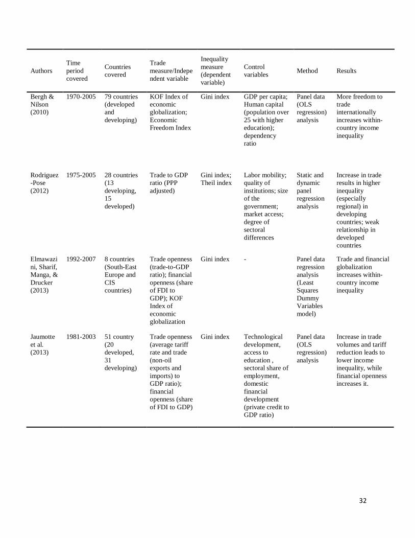
32
Authors
Time
period
covered
Countries
covered
Trade
measure/Indepe
ndent variable
Inequality
measure
(dependent
variable)
Control
variables Method Results
Bergh &
Nilson
(2010)
1970-2005 79 countries
(developed
and
developing)
KOF Index of
economic
globalization;
Economic
Freedom Index
Gini index GDP per capita;
Human capital
(population over
25 with higher
education);
dependency
ratio
Panel data
(OLS
regression)
analysis
More freedom to
trade
internationally
increases within-
country income
inequality
Rodriguez
-Pose
(2012)
1975-2005 28 countries
(13
developing,
15
developed)
Trade to GDP
ratio (PPP
adjusted)
Gini index;
Theil index
Labor mobility;
quality of
institutions; size
of the
government;
market access;
degree of
sectoral
differences
Static and
dynamic
panel
regression
analysis
Increase in trade
results in higher
inequality
(especially
regional) in
developing
countries; weak
relationship in
developed
countries
Elmawazi
ni, Sharif,
Manga, &
Drucker
(2013)
1992-2007 8 countries
(South-East
Europe and
CIS
countries)
Trade openness
(trade-to-GDP
ratio); financial
openness (share
of FDI to
GDP); KOF
Index of
economic
globalization
Gini index - Panel data
regression
analysis
(Least
Squares
Dummy
Variables
model)
Trade and financial
globalization
increases within-
country income
inequality
Jaumotte
et al.
(2013)
1981-2003 51 country
(20
developed,
31
developing)
Trade openness
(average tariff
rate and trade
(non-oil
exports and
imports) to
GDP ratio);
financial
openness (share
of FDI to GDP)
Gini index Technological
development,
access to
education ,
sectoral share of
employment,
domestic
financial
development
(private credit to
GDP ratio)
Panel data
(OLS
regression)
analysis
Increase in trade
volumes and tariff
reduction leads to
lower income
inequality, while
financial openness
increases it.

33
2.5 Theoretical expectations
This chapter aimed at answering the first research sub-question, which was done by reviewing the
theories and evidence present in the literature analysing trade-inequality relationship in developing
and developed countries. At first the reader was introduced with three theories that provide
different assumptions regarding the trade impact on income distribution– the HOS model,
convergence theory and dependency theory. The HOS model predicts that with trade expansion,
within-country income inequality in the developing world would decline, while the opposite trend
is expected in developed countries. Similarly, according to the convergence theory, more trade
would be more beneficial for developing countries and lead to higher economic growth and lower
inequality. However, in the reviewed empirical studies such theoretical assumptions received very
little support. One of the possible reasons is that theoretical predictions assume certain conditions
(like full employment in HOS model), that need to be fulfilled in order for the theory to hold.
In contrast, according to theoretical implications derived from the dependency theory, more trade
brings benefits only for the developed world, while developing countries suffer from exploitation
and face barriers to further development. Consequently, trade expansion would only increase
inequality in the developing world. A number of reviewed studies show support for the
assumptions provided by the dependency theory, as indeed, in many instances trade liberalisation
was found to be related to rising income gap in developing countries. Likewise, the same
conclusion could be made from the further evidence discussed and the presented summarizing
table, where in majority of cases, trade induced increase in inequality was observed. On the other
hand, based on existent mixed results regarding trade-inequality effects in developed countries, it
can be stated that developed world is less vulnerable to the impact of trade expansion in terms of
income distribution (as in several studies reviewed, weak, or no relationship between trade
expansion and within-country income inequality was observed).
Therefore the theoretical expectations of this research follow the predictions of the dependency
theory and it is expected that developing countries are more vulnerable to increase in trade and
thus will face higher within-country inequality as compared to developed world. In addition, as
theory suggests, more trade can even be beneficial to the developed countries in terms of income
distribution. Consequently, the following hypothesis is formulated:

34
H: Trade expansion increases income inequality in developing countries, but not in developed
countries.
Due to possible differences in trade impact on inequality, the expected relationships for developing
and developed countries are illustrated in figure 1 and 2 accordingly. In addition, as discussed in
section 2.3, there are other factors that are said to have an effect on inequality levels in both
developing and developed world (institutional effectiveness, democracy, government spending
and population growth), and thus such factors are included into the model of this research as
controls. All the expected relationships are presented in two figures below:
Figure 1
Developing countries
• + trade expansion
• - effective institutions
• - democracy
• - government expenditure
• + population growth rate
Within-country income inequality

35
Figure 2
Developed countries
• +/- trade expansion
• - effective institutions
• - democracy
• - government expenditure
• + population growth rate
Within-country income inequality

36
3. Research design
The purpose of this chapter is to answer the second research sub-question presented in chapter 1:
How can the variables be operationalized and how can trade-inequality effects be researched?
This is done by first of all presenting the chosen research design and the models (regression
equation for the base model, the main model, and the model used as a robustness check). Then the
dependent, independent and control variables are operationalized and the selected measurements
are explained together with the data sources. Afterwards the sample of countries is presented. At
the end of the chapter validity and reliability of chosen research design and selected indicators is
discussed.
3.1 Empirical methods
In order to answer the central research question and test the hypothesis regarding the differences
in trade-inequality effects, a longitudinal observational study design is chosen. In observational
study design, researchers do not have control over independent variables and thus use the observed,
or measured values of the variables (X) reflecting real life situations (Kellstedt & Whitten, 2013).
Consequently, the results of observational studies are often considered to be more credible.
Additionally, in order to examine trade-inequality relationship and to see whether changes in trade
levels result in changes in inequality over time, panel data analysis will be conducted. More
specifically, a regression analysis using balanced panel data (consisting of multiple observations
over time for each country included into the sample (N)) will be performed. The benefits of panel
data analysis are numerous: it allows to have considerably larger data sets, to capture and estimate
additional effects, that are often not observed using other types of data (pure time-series, or cross-
section), in addition, in panel data analysis lower collinearity and more variability among the
variables could be anticipated (Lewis-Beck, Bryman, & Liao, 2004).
Bivariate regression analysis is a commonly used technique when aiming to examine the
relationship between the dependent (Y) and independent (X) variables. Yet, in order to control for
the possible effects of additional factors (control variables) on the dependent variable (Y), a
multivariate regression analysis is a better alternative (Lewis-Beck, Bryman, & Liao, 2004). In
order to conduct a linear regression analysis several assumptions have to satisfied: the sample size
(N) should be sufficiently large; the relationship between the dependent and independent variables

37
should be as linear as possible; the measurements of all the variables should be accurate and
quantitative (interval or ratio variables); independent variables cannot be linearly related to other
independent variables (no multicollinearity); the variables should have normal distribution (Lewis-
Beck, Bryman, & Liao, 2004). Additionally, there should be no heteroscedasticity. As it is shown
in the following parts of this chapter, several of these conditions are already satisfied: the sample
of this research is considered to be large enough (including as many countries as possible into the
sample), moreover, all the variables are either ratios, or intervals. In chapter 4 it will be checked
whether other conditions are as well met.
As it was already stated in the introductory chapter, one of the aims of this research is to contribute
to the existing pool of literature by analysing the latest data available. Additionally, in order to
observe the changes in patterns of trade-inequality relationship and better capture the effects of
trade expansion on levels of inequality in countries on different stage of development, it is
important to have a longer time frame with multiple observations for each country, as all the
variables included into this research vary over time. Consequently this analysis covers annual data
for a 10 year period, from 1999 to 2008. Both boundaries of the time frame are set based on data
availability, as a number of sources provide rather scarce data for developing countries, or lack
several observations, which then serves as an obstacle to extending both the time period and the
country sample of this research. In total the dataset used for this research consists of 910
observations (10 yearly observations for each country (N=91)).
The analysis will be conducted using GRETL econometric software. The variables included into
the main model will be employed in order to run a regression using several different econometric
models (pooled Ordinary Least Squares (OLS), fixed effects, random effects, or Weighted Least
Squares (WLS)). In turn, the best fit model will be chosen and the results commented.
Additionally, robustness check will be performed in order to check whether the obtained results
change once the model is modified.
The base model with all the variables (that are operationalized in further parts of this chapter) is
now be presented:
1) 𝐺𝑖𝑛𝑖𝑖𝑡 = 𝛽0 + 𝛽1𝑇𝐺𝐷𝑃𝑖𝑡 + 𝛽2𝐷𝐸𝑀𝑖𝑡 + 𝛽3𝐺𝐸𝑖𝑡 + 𝛽4𝐺𝑂𝑉𝑆𝑖𝑡 + 𝛽5𝑃𝑔𝑟𝑜𝑤𝑡ℎ𝑖𝑡 + 𝛽6𝐷𝑒𝑣𝐷𝑢𝑚𝑚𝑦 +
𝛽𝑘𝑋𝑘 + 𝜀𝑖𝑡

38
Where ‘I’ denotes the number of a country, I = [1…. n], and‘t’ denotes a given year t = [1….10]
GINI -> GINI coefficient;
TGDP -> trade to GDP ratio;
DEM -> democracy score
GE -> government effectiveness
GOV -> government spending;
Pgrowth -> population growth rate
DevDummy -> development dummy (level of economic development)
It is important to note that in the presented base model, the effects of trade expansion and level of
economic development on inequality are measured separately (for each variable). Yet, the goal of
this research is to identify the differences in trade effects on levels of inequality depending on a
stage of development, as presented at the end of chapter 2. Consequently, the difference between
developed and developing countries needs to be established. One way to do that is to analyse both
groups of countries separately and to compare the obtained results. Another option is to analyse
the full sample of countries introducing an interaction term (interacting trade and development
variables) for the purpose of country distinction into two groups. The advantage of analysing the
full sample is that it allows to measure whether the possibly existent differences in trade-inequality
effects between developed and developing countries are significant. Therefore, to better reflect the
theoretical expectations of this research, an interaction term (INTER) is introduced to the main
model; it is constructed by multiplying the trade-to-GDP ratio (TGDP) and dummy variable
representing the stage of economic development (constructed based on World Bank’s country
classification). Consequently, it is expected that having this interaction term (were trade-to-GDP
interacts with the level of development) as independent variable would help to identify differences
in trade-inequality effects by group (depending on level of development) in a dichotomous way.
Further variable explanations are provided in the operationalization part. It is important to note
that during the course of empirical research, the main regression equation is employed when
certain tests need to be conducted (for instance when testing for heteroscedasticity). The main
model of this research is thus the following:
2) 𝐺𝑖𝑛𝑖𝑖𝑡 = 𝛽0 + 𝛽1𝐼𝑁𝑇𝐸𝑅𝑖𝑡 + 𝛽2𝑇𝐺𝐷𝑃𝑖𝑡 + 𝛽3𝐷𝐸𝑀𝑖𝑡 + 𝛽4𝐺𝐸𝑖𝑡 + 𝛽5𝐺𝑂𝑉𝑆𝑖𝑡 + 𝛽6𝑃𝑔𝑟𝑜𝑤𝑡ℎ𝑖𝑡 +
𝛽7𝐷𝑒𝑣𝐷𝑢𝑚𝑚𝑦 + 𝛽𝑘𝑋𝑘 + 𝜀𝑖𝑡
39
Where ‘I’ denotes the number of a country, I = [1…. n], and‘t’ denotes a given year t = [1….10]
INTER -> interaction term (1) (product of TDGP and development dummy variable)
Additionally, in order to check whether model estimates change when another measurement of
economic development is employed, a robustness check is conducted. Thus for the purpose of this
test, another interaction term (INTER2) is constructed. The components of the second interaction
term are trade-to-GDP ratio (TGDP) and GDP per capita variable. The difference between the two
pairs of interacting variables is that instead of looking for differences in trade-inequality effects
depending on which group a country belongs to, an interaction with GDP per capita component
allows to check whether the differences in such effects depend on how rich or poor a country is.
Alternative models used for robustness check are specified below (both the base model without
interaction term (3) and with the added second interaction term (4)):
3) 𝐺𝑖𝑛𝑖𝑖𝑡 = 𝛽0 + 𝛽1𝑇𝐺𝐷𝑃𝑖𝑡 + 𝛽2𝐷𝐸𝑀𝑖𝑡 + 𝛽3𝐺𝐸𝑖𝑡 + 𝛽4𝐺𝑂𝑉𝑆𝑖𝑡 + 𝛽5𝑃𝑔𝑟𝑜𝑤𝑡ℎ𝑖𝑡 + 𝛽6𝐺𝐷𝑃𝑐𝑎𝑝 +
𝛽𝑘𝑋𝑘 + 𝜀𝑖𝑡
4) 𝐺𝑖𝑛𝑖𝑖𝑡 = 𝛽0 + 𝛽1𝐼𝑁𝑇𝐸𝑅2𝑖𝑡 + 𝛽2𝑇𝐺𝐷𝑃𝑖𝑡 + 𝛽3𝐷𝐸𝑀𝑖𝑡 + 𝛽4𝐺𝐸𝑖𝑡 + 𝛽5𝐺𝑂𝑉𝑆𝑖𝑡 + 𝛽6𝑃𝑔𝑟𝑜𝑤𝑡ℎ𝑖𝑡 +
𝛽7𝐺𝐷𝑃𝑐𝑎𝑝 + 𝛽𝑘𝑋𝑘 + 𝜀𝑖𝑡
Where ‘I’ denotes the number of a country, I = [1…. n], and‘t’ denotes a given year t = [1….10]
GDPcap -> GDP per capita
INTER2 -> second interaction term (product of TDGP and GDP per capita variables)
3.2 Operationalization
Having introduced the models, in this part the independent, dependent and control variables
included into the research are defined, the measurements explained and the choice of the data
sources are justified.
3.2.1 Dependent variable (Y)
The dependent variable of this research is within-country inequality. Due to the fact that the
concept of inequality as such is hard to measure, for the purpose of this research Gini index is used
as the closest proxy for the dependent variable (within-country inequality). The index shows how
the income (or expenditure on consumption) is distributed among households, or individuals

40
within a country and how it diverges from perfectly equal income distribution. The values of Gini
index range from 0 (representing perfect equality where all individuals, or households within a
country get the same income) to 1 (representing perfect inequality, where all the income is owned
by one individual/household). Alternatively the 0-100 scale for Gini index values is often used.
The graphical representation of Gini index is known as the Lorenz curve of income distribution,
where the value of Gini index is basically the area between the Lorenz curve and the line
representing perfectly equal income distribution (Darity, 2008). When the income is equally
distributed, Lorenz curve and perfect equality curve becomes the same, in which case the value of
Gini index is 0. This index is considered to be the most widely used measurement of income
inequality which is also evident from the summary presented in table 1, where the vast majority of
scholars chose this index while analysing the patterns of income distribution.
As Korzeniewicz & Moran (2009) state, Gini index satisfies the conditions crucial for inequality
measurement: its values are symmetrical and constrained by the lower and upper boundaries and
also, its values are said to reflect changes in redistribution from rich to poor individuals (Pigou-
Dalton principle of transfers). In addition, choosing this measurement as a dependent variable for
the purpose of this research is considered to be appropriate as according to Rudra (2004) such
calculated measures of inequality allows to see whether the poorest part of the society is in a better
or worse position in terms of within-country income distribution. Consequently, it will be possible
to make implications regarding the trade-inequality effects and to see whether more trade brings
more gains, or losses for the poorest segments in both developed and developing countries. The
data on Gini index for this research is taken from the Standardized World Income Inequality
Database (SWIID). The database includes data from sources like World Income Inequality
Database, OECD Income Distribution Database, Eurostat and many more (Solt, 2009). In addition,
out of all the alternative options, the SWIID offers the widest coverage (in terms of number of
countries and years) and highest comparability, thus it is considered to be a highly suitable choice
for inequality studies (Solt, 2009). The SWIID was also used for inequality measure in a number
of studies reviewed in literature review part (Bergh & Nilsson, 2010).
Furthermore, in inequality studies, authors alternatively use other measures, such as Theil
coefficient, or look at the share of income received by the highest and lowest quintiles/deciles in
the population (Bussmann, Soysa, & Oneal, 2005; Rodriguez-Pose, 2012). Regarding the Theil
41
coefficient, it is not used as commonly as the Gini index mainly because the data sources for this
coefficient are lacking, moreover, its interpretation is not as easy and straightforward
(Korzeniewicz & Moran, 2009). As for the income shares, in general more data is available for
developed countries and not for developing countries, which is a considerable limitation
considering the aim of this study.
3.2.2 Independent variable (X)
As shown in the main model equation (2), the variable of interest in this research is interaction
term (INTER). One of the components of the interaction is the variable representing trade openness
- trade-to-GDP ratio (TGDP). This ratio shows the share of trade volumes (the sum of exports and
imports of goods and services) to GDP and is also a common choice of scholars researching trade-
inequality relationship (summary table 2.4). In addition, trade-to-GDP ratio is considered to be a
measurement of de facto trade/economic openness and integration into the global economy,
showing how important country’s exports and imports are (Jaumotte, Lall, & Papageorgiou, 2013;
Bussmann, Soysa, & Oneal, 2005). However, it is important to note, that the values of this indicator
are said to be affected by additional factors, such as trade policy, structure of country’s economy,
or even country size and geographical location (Bussmann, Soysa, & Oneal, 2005). Yet, based on
the studies reviewed in chapter two, it is evident that trade-to-GDP ratio is so far the most often
used measure of trade openness and expansion. The data for this variable is obtained from the
World Bank’s World Development Indicators (WDI) database.
The second component of the interaction term is development dummy variable. Adding a dummy
in order to divide country sample into two distinct groups is a common practice in regression
analysis. Moreover, using a categorical variable appropriately addresses both the central research
question and the hypothesis, where both groups of countries (developed and developing) are
named. Therefore, following Rodriguez-Pose, (2012) a proxy (dummy) variable for the state of
development is introduced, where developing countries are assigned a value of 0 and developed
countries a value of 1. However it is important to note that there also exist certain limitations of
using dummy variables. More specifically some information might be lost, as for instance when
assigning countries to the same category, existent differences between those countries (if any)
would not be reflected. One of the solutions could be using an interval level measurement for the
state of development, yet alternatively it is expected that any relationships that could be

42
unobserved when using the dummy variable for the purpose of country division, will eventually
be revealed when conducting a robustness check with an alternative measure of the level of
development (explained later in this section).
For the purpose of dividing countries into two groups (developed countries and developing
countries) country classification provided by the World Bank is used. Here based on the income
levels (GNI per capita) countries are assigned to one of the following groups: low income
economies, lower middle income economies, upper middle income economies, high income
economies, or high income OECD members (The World Bank, 2016)1. Consequently, all countries
belonging to the low or middle income groups are considered to be developing, while high income
countries are assigned to the category of developed states (The World Bank, 2016). Also, as noted
by the World Bank, although the explained country division into developed and developing group
is frequently used, it does not necessarily mean that all the countries assigned to a particular group
are on the same stage of development, which indicates that there are certain limitations regarding
such country division. However, due to the fact that the World Bank country classification is
widely acknowledged and used in the academic literature, it is also considered to be an appropriate
choice for the purpose of this research.
It is important to note, that for this research countries included into the sample are divided into two
categories (developed or developing country group) based on the World Bank Analytical
Classification during the entire time frame of the analysis, and thus cases where a country advances
to the category of developed states (or from upper middle income to high income according to
World Bank’s classification) are taken into account. Instances of such countries are the following:
Croatia (2008), Czech Republic (2006), Estonia (2006), Hungary (2007), Republic of Korea
(2001), and Slovak Republic (2007). A possible solution in this situation is to assign country to a
group to which it was attributed for a longer period during the time frame of the analysis.
(Rodriguez-Pose, 2012). Consequently, from all the cases that were mentioned, Republic of Korea
1 As the World Bank defines, countries with GNI per capita not exceeding the amount of $1,045 are considered to be low income economies. Middle income economies then are defined as having the GNI per capita between $1,045 and $12,736, where the lower-middle income countries are separated from the upper-middle income countries at the level of $4,125. Finally, countries with GNI per capita equal to $12,736 or more are considered to be high income economies. (The World Bank, 2016)

43
is assigned to the category of developed states for the entire time period of this research, while
other countries stay in the category of developing states.
Consequently, both of the described variables (trade-to-GDP ratio and development dummy) are
multiplied and the independent variable of this research – the interaction term is constructed. It is
important to mention that both of the components are also separately added to the main model. In
general, interaction term is used in cases where it is assumed that the impact of one independent
variable might be dependent on another independent variable. The significance and negative
coefficient signs of the model estimates for interacting trade-to-GDP and development dummy
variable would then indicate that the more developed a country is, the more likely trade expansion
is to reduce inequality. In contrast, in case of less developed countries (developing world) this
would serve as an indication that trade expansion is less likely to lower the levels of inequality. In
turn, this would signal that the expected differences in trade-inequality effects in developed and
developing world indeed exist, which then results in confirming the hypothesis presented at the
end of chapter 2.
Furthermore, for the purpose of robustness check, the main model is modified by using an
alternative interaction term (INTER2) as an independent variable. The second interaction consists
of previously described trade-to-GDP variable and GDP per capita variable. GDP per capita is an
alternative measure of the level of country’s economic development, which is commonly
accounted for when analysing trade-inequality relationship (refer to table 1) (Bergh & Nilsson,
2010; Rudra, 2004; Meschi & Vivarelli, 2008). Adding trade-to-GDP and GDP per capita
interaction to the analysis when testing for robustness should reveal whether trade-inequality
relationship is more pronounced in richer, or poorer countries. In other words, it is expected that
changing the categorical component (development dummy) of an interaction term with GDP per
capita variable would allow to check whether the more developed a country is, the lower the
likelihood that trade expansion increase inequality, or not. Data for this variable (GDP per capita
(current US$)) is gathered from the WDI database.
3.2.3 Control variables
At the end of chapter two, the reader was presented with several other factors that are said to have
an effect on within-country inequality and thus were previously included into the analyses made

44
by other researchers. All of these factors (democracy, effectiveness of domestic institutions,
population growth rate and government spending) are included into the model as control variables.
Controlling for variables that presumably have an effect on dependent variable (Y) is important
for the results of the analysis, as otherwise the obtained estimates might show spurious
relationships and thus lead to misleading interpretations (Punch, 1998). Due to the fact that
variables like democracy or effectiveness of institutions are difficult to measure, proxy indicators
are chosen.
Democracy (DEM)
For the purpose of this research, the proxy indicator chosen to measure the strength of democratic
regime are the polity scores provided in Polity IV Project dataset. This measurement is a common
choice in inequality studies, as currently the dataset provides annual time-series data for 167
countries during the period from 1946-2013. The characteristic of political regimes and institutions
are annually assessed, thus the dataset is regularly updated. Country’s level of democracy is
evaluated based on the process of executive recruitment (its openness and competitiveness),
political participation, competition and the existent constraints (checks) on the executive. The
polity, or democracy score values range from -10 (authoritarian countries) to +10 (pure,
consolidated democracies). However, when converting the scores into regime categories,
autocracies score from -10 to -6, anocracies (partly dictatorship, partly democracy) from -5 to +5,
while democracies from +6 to +10 (Centre for Systematic Peace, 2016).
Government effectiveness (GE)
As it was explained in sub-chapter 2.3, effectiveness of domestic public institutions is said to be
an important factor affecting trade-inequality outcomes, especially with regards to developing
world, and thus it is important to include it into the analysis. Consequently, the chosen proxy
measurement is the government effectiveness index from the Worldwide Governance Indicators.
This index is said to reflect the degree of perceived quality of public and civil services, the level
of independence from various pressures, quality of policy making process, government’s
involvement and commitment to it (Kaufmann & Kraay, 2016). In addition, the measurement is
composed using variables from a large number of representative and non-representative sources.
Similarly to other WGI indicators, the government effectiveness index can be presented in two
ways: in the units with values ranging from -2.5 (low effectiveness) to +2.5 (high effectiveness),
45
or in percentage terms ranging from 0 (low effectiveness) to 100 (high effectiveness) (Kaufmann
& Kraay, 2016). Due to the fact that between 1996 and 2002 the values for government
effectiveness index (as well as for other WGI) were presented every 2 years, in this research the
years when the index is missing are assigned with values of previous year. This is considered to
be a reasonable solution as in general no major changes were observed during the short term
periods (1-2 years) thus the missing values are very likely to be similar to the year before.
However it is important to note, that the government effectiveness index and WGI in general have
certain limitations. For instance, as WGI critics argue, due to a variety of data sources that are used
to construct the indicators, these measures lack comparability over time, meaning that WGI might
not be the best choice when aiming to compare multiple countries during multiple point in time.
In addition to that, the WGI are said to lack transparency, as some of the data sources are unclear,
or inaccessible to others. Finally, the WGI are rescaled resulting in exactly the same averages
(global) during every period of time which is said to have an effect on comparability over time.
On the other hand, in their answer to critics, authors of the WGI argue that their methodology
allows to combine the data obtained from diverse sources and to make the indicators comparable
(Kaufmann, Kraay, & Mastruzzi, 2007). Moreover, when it comes to transparency related critique,
authors note that national assessments are often not available to the general public (Kaufmann,
Kraay, & Mastruzzi, 2007).
Government spending (GOVS)
The levels of government expenditure (on health and education) is another crucial factor that needs
to be accounted for in this research, as high levels of spending are said to be helpful reducing the
income gap between rich and poor members of the society (for more explanations refer to 2.3).
However, due to limited data availability, it is decided to use spending on health as a proxy variable
for governmental spending on both education and health. The positive relationship between both
types of spending has been observed in the literature (Rahman, 2011; Al-shihri, 2014), thus it can
be implied that countries that spend more on education, will also have high expenditure on
healthcare. Consequently, spending on health is considered to be an appropriate proxy for both
types of government expenditure. Yet, it is still crucial to note that since proxy variable is not a
direct measure (of spending on education in this case), certain limitations exist.

46
Health spending variable used for the purpose of this research represents a share of GDP spent on
healthcare. The data for this variable is taken from the WDI database where the World Bank
provides estimated weighted averages based on data from World Health Organization Global
Health Expenditure Database.
Some researchers alternatively use the data provided in the International Monetary Fund’s
Government Finance Statistics (GFS) dataset which also provides figures for different types of
social spending (health, education, social protection) (Rudra, 2004). However, compared to GSF,
the WDI data on government expenditure covers more countries during the time period of this
analysis, which allows to include spending variable without significantly reducing the country
sample.
Population growth (Pgrowth)
Another variable added to the model as a control is population growth rate. As it was previously
explained, controlling for this factor is important, as high population growth rates are said to be
related to higher levels of inequality. This factor was also controlled for in other researches (refer
to summary table 1). The data for this control variable is gathered from the WDI database where
the annual population growth rate (%) is provided.
3.3 Country sample
A considerable drawback currently existent in the literature on trade-inequality relationship is the
fact that the vast majority of studies focus more on developed countries (Rodriguez-Pose, 2012).
This is commonly explained by the limited data availability for developing world. Consequently,
as it was already noted, the findings so far are not unified and thus it remains unclear which
countries are more vulnerable to the effects of trade expansion on income inequality. In order to
overcome this drawback and to obtain more generalizable results, this analysis covers a country
sample in which developing and developed countries are about equally represented. It is expected
that having a country sample that accurately represents both groups of countries would make it
easier to observe the differences in trade effects in developed and developing world.
A number of countries were not included into the sample due to the lack of data for the time period
of analysis. The final country set consists of 91 countries, where 63 are developing states and 28
are developed states. A table with full list of countries can be found in appendix 1. The final
47
country division based on the previously explained World Bank’s country classification is
provided in appendix 2.
3.4 Reliability and validity
Reliability and validity are the two principles significantly important in terms of associating
theoretically defined concepts with particular empirical indicators and empirically analysing
certain phenomenon (Lewis-Beck, Bryman, & Liao, 2004). As Kellstedt & Whitten (2013)
explain, the measures used for evaluating causal relationships and testing hypothesis have to be
both reliable and valid. More specifically, the combination of reliable, but invalid measure is not
considered to be useful in terms of hypothesis testing, while unreliable measures cannot result in
reliable hypothesis testing (Kellstedt & Whitten, 2013). Consequently, both of the features were
taken into account when choosing the operational measures for the concepts defined while
discussing the relationship between trade and inequality in developed and developing world.
The main requirements for a measure and thus the results to be reliable are the following: it has to
be equivalent and repeatable, implying that the same, or very similar results should be obtained if
choosing the same or even an alternative measure; in addition, the observations have to consistent
in time and space (Lewis-Beck, Bryman, & Liao, 2004; Kellstedt & Whitten, 2013). Therefore,
the indicators chosen to measure the dependent, independent and control variables in this research
are annually calculated using the same methodology and considered to be stable, which implies
that the same results could be anticipated if repeating the analysis for the second time. The only
exception regarding methodology is the government effectiveness index, which limitations where
already discussed in the operationalization part. In addition to that, the data sources for measuring
all the variables were chosen based on the previous choices made by other researchers focusing on
trade-inequality relationship, which also serves as an indication of reliability, as data is obtained
from widely acknowledged sources.
Regarding the validity principle, it firstly refers to the extent to which chosen indicators accurately
measure the theoretical concepts that they intend to measure (Lewis-Beck, Bryman, & Liao, 2004;
Kellstedt & Whitten, 2013). A number of indicators chosen for the purpose of this analysis are
direct measures of certain concepts (trade levels, government spending), meaning that the exact
calculated numbers, or levels are used, while for the remaining ones (levels of inequality,
democracy, effectiveness of institutions, democracy) the closest proxies and the most commonly

48
used measures were selected. Hence, one of the validity conditions is satisfied. Another
requirement for internal validity is existence of causal relationship between the independent and
dependent variables (Trochim, 2000). The existence of trade-inequality relationship has been
discussed by a number of theories and observed in studies reviewed in chapter 2, in addition to
that, this research controls for additional factors that might affect levels of within-country
inequality. Furthermore, the external validity shows if the results obtained are generalizable to a
broader population. This research aims to achieve external validity by covering a representative
sample of countries belonging to two groups (developed countries and developing countries) and
thus it is expected that the obtained results will be generalizable even for those countries, that due
to lack of data availability were not included into the sample. In addition, having representative
sample it is expected that the findings indicating certain differences in terms of trade-inequality
effects in countries on different stage of development would be thus applicable for the entire group
(developed or developing world).

49
4. Empirical analysis
In this chapter following the detailed explanations provided in the research design part (chapter 3)
further steps of the analysis are presented and discussed. Consequently, this part aims to answer
the third research sub-question presented in chapter 1:
What are the results of the analysis?
The chapter is structured as follows: firstly, the descriptive statistics of all the variables are
provided and it is further checked whether the remaining preconditions for conducting a regression
analysis are satisfied (as discussed in chapter 3 it is checked whether there is no problem of
multicollinearity, heteroscedasticity, whether the variables are normally distributed and there is a
linear relationship between X and Y); then the best fit model is selected out of for alternative
econometric models (pooled OLS, fixed effects, random effects, or WLS); finally, the estimates
of the most suitable model are analysed and commented looking at the obtained significance of
the model, variables and coefficients. Additionally, a robustness check is performed in order to
test whether the obtained estimates change when the model is modified.
4.1 Descriptive statistics
Before proceeding to regression models it is important to look at the descriptive statistics of the
panel dataset and make some general conclusions about the data that is used for the purpose of this
analysis. Table 2 provides summary statistics for all the variables that will be included into the
regression models (both the main model and the one used for robustness check). It is important to
note that interaction variables are not included into the table, yet the descriptive statistics for the
components are provided. Based on the information presented in the table it can firstly be stated
that the analysis will be conducted using balanced panel data, as there are no missing observations.
Additionally the mean and the median of the variables should be looked at, as based on the
difference between the two values, implications regarding the distribution of the variables can be
made. The mean is calculated by dividing the sum of all the observations by the number of
observations, while the median is the middle value of all the variable values ordered from the
lowest to the highest numerical value (Weiss, 2008). When the values of the mean and median are
equal, the variables are said to have a symmetric (and normal) distribution (Pfaffenberger &
Patterson, 1987). In contrast, when the values are not equal, or close to equal, the distribution is
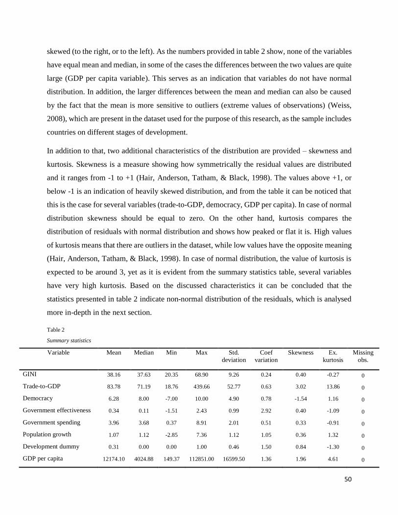
50
skewed (to the right, or to the left). As the numbers provided in table 2 show, none of the variables
have equal mean and median, in some of the cases the differences between the two values are quite
large (GDP per capita variable). This serves as an indication that variables do not have normal
distribution. In addition, the larger differences between the mean and median can also be caused
by the fact that the mean is more sensitive to outliers (extreme values of observations) (Weiss,
2008), which are present in the dataset used for the purpose of this research, as the sample includes
countries on different stages of development.
In addition to that, two additional characteristics of the distribution are provided – skewness and
kurtosis. Skewness is a measure showing how symmetrically the residual values are distributed
and it ranges from -1 to +1 (Hair, Anderson, Tatham, & Black, 1998). The values above +1, or
below -1 is an indication of heavily skewed distribution, and from the table it can be noticed that
this is the case for several variables (trade-to-GDP, democracy, GDP per capita). In case of normal
distribution skewness should be equal to zero. On the other hand, kurtosis compares the
distribution of residuals with normal distribution and shows how peaked or flat it is. High values
of kurtosis means that there are outliers in the dataset, while low values have the opposite meaning
(Hair, Anderson, Tatham, & Black, 1998). In case of normal distribution, the value of kurtosis is
expected to be around 3, yet as it is evident from the summary statistics table, several variables
have very high kurtosis. Based on the discussed characteristics it can be concluded that the
statistics presented in table 2 indicate non-normal distribution of the residuals, which is analysed
more in-depth in the next section.
Table 2
Summary statistics
Variable Mean Median Min Max Std.
deviation
Coef
variation
Skewness Ex.
kurtosis
Missing
obs.
GINI 38.16 37.63 20.35 68.90 9.26 0.24 0.40 -0.27 0
Trade-to-GDP 83.78 71.19 18.76 439.66 52.77 0.63 3.02 13.86 0
Democracy 6.28 8.00 -7.00 10.00 4.90 0.78 -1.54 1.16 0
Government effectiveness 0.34 0.11 -1.51 2.43 0.99 2.92 0.40 -1.09 0
Government spending 3.96 3.68 0.37 8.91 2.01 0.51 0.33 -0.91 0
Population growth 1.07 1.12 -2.85 7.36 1.12 1.05 0.36 1.32 0
Development dummy 0.31 0.00 0.00 1.00 0.46 1.50 0.84 -1.30 0
GDP per capita 12174.10 4024.88 149.37 112851.00 16599.50 1.36 1.96 4.61 0

51
4.2 Testing the assumptions of multivariate regression analysis
4.2.1 Normality
Normality is considered to be one of the fundamental assumptions that have to be satisfied in order
to conduct a multivariate regression analysis (Hair, Anderson, Tatham, & Black, 1998). More
specifically it is crucial that the variables included into the model would have normal, or close to
normal distribution. The concept of normal distribution is defined as: “a bell-shaped statistical
distribution that can be entirely characterized by its mean and standard deviation” (Kellstedt &
Whitten, 2013, p. 143). In order to test each of the variables for normality, statistical and graphical
methods are used. More specifically, for every variable a histogram comparing the observed values
with values in case of normal distribution is checked and additionally, results of normality tests
conducted in GRETL, as well as previously discussed values of mean, median, skewness and
kurtosis are looked at. In case the values of the variables are not normally distributed, a number of
transformation options are considered and the transformation which improves residual distribution
the most is presented and used further on in the analysis.
Dependent variable (Y)
As it is shown in graph 1, the values of the dependent variable of this research (Gini index) are not
normally distributed. Consequently, a transformation is needed. During the process of
normalization, a number of possible data transformations (logarithmic, square root, different
exponentiation variants) were made. Transforming the values of the dependent variable by using
the exponent of 1/3 was found to be improving the distribution of this variable the most, as
compared to other possible transformations. Frequency distribution histogram for the transformed
variable is provided in graph 2. The results of the normality tests are shown in table 3.
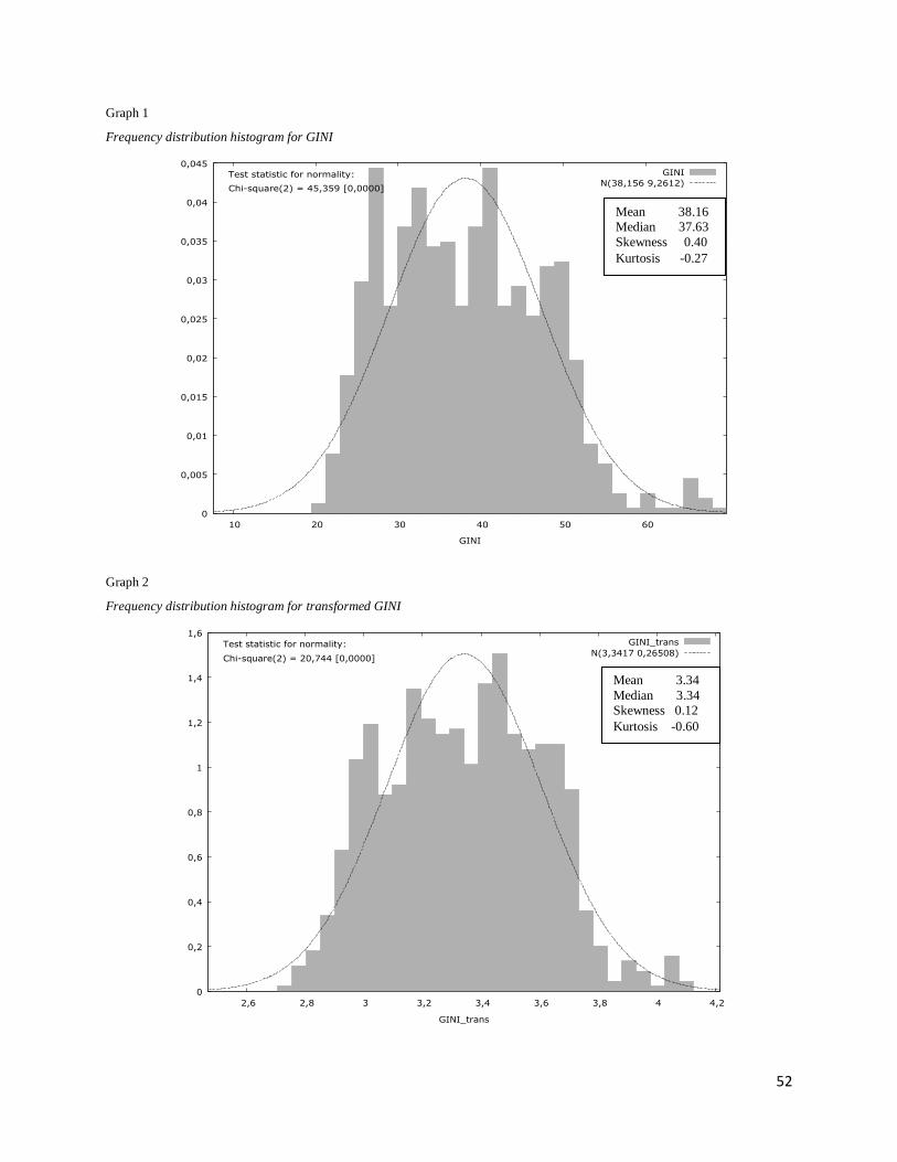
52
Graph 1
Frequency distribution histogram for GINI
Graph 2
Frequency distribution histogram for transformed GINI
0
0,005
0,01
0,015
0,02
0,025
0,03
0,035
0,04
0,045
10 20 30 40 50 60
Densi
ty
GINI
GINI
N(38,156 9,2612)Test statistic for normality:
Chi-square(2) = 45,359 [0,0000]
0
0,2
0,4
0,6
0,8
1
1,2
1,4
1,6
2,6 2,8 3 3,2 3,4 3,6 3,8 4 4,2
Density
GINI_trans
GINI_trans
N(3,3417 0,26508)Test statistic for normality:
Chi-square(2) = 20,744 [0,0000]
Mean 3.34
Median 3.34 Skewness 0.12
Kurtosis -0.60
Mean 38.16
Median 37.63
Skewness 0.40
Kurtosis -0.27

53
Table 3
Results of the normality tests
Test GINI
p- value
GINI (transformed)
p-value
Doornik-Hansen test 1.41381e-010 3.12893e-005
Shapiro-Wilk W 1.24181e-011 1.17124e-007
Lilliefors test 0 0
Jarque-Bera test 1.19281e-006 0.0003729
Independent variable (X)
As it was explained, the independent variable of this research is an interaction term which consist
of two variables – trade-to-GDP ratio and the development dummy variable. Consequently, in
order for the interaction term to have normal distribution, it is important that the values of the
components are normally distributed. The development dummy variable is dichotomous (as
variable has only two values 1, or 0) and cannot be transformed for normality. However referring
to the summary statistics table (table 2) it could be stated that the variable has close to normal
distribution, as the difference between mean and median is not large, also neither skewness, nor
kurtosis values are extremely high, or low. On the other hand, when more normality cannot be
achieved with the means of transformations, it is better to use the original variable (Hair, Anderson,
Tatham, & Black, 1998).
Regarding the second component, as the frequency distribution histogram (graph 3) indicates, the
values of trade-to-GDP variable are not normally distributed, and thus a transformation is needed.
The best results in terms of normality are obtained by using the exponent of (-1/5) (graph 4).
Results of normality tests are compared in table 4.

54
Graph 3
Frequency distribution histogram for trade-to-GDP
Graph 4
Frequency distribution histogram for transformed trade-to-GDP
0
0,002
0,004
0,006
0,008
0,01
0,012
0,014
0 100 200 300 400
Densi
ty
TGDP
TGDP
N(83,777 52,771)Test statistic for normality:
Chi-square(2) = 1655,540 [0,0000]
0
2
4
6
8
10
12
0,3 0,35 0,4 0,45 0,5 0,55
Densi
ty
TGDP_trans
TGDP_trans
N(0,42652 0,043647)Test statistic for normality:
Chi-square(2) = 5,863 [0,0533]
Mean 83.78
Median 71.19
Skewness 3.02
Kurtosis 13.86
Mean 0.43
Median 0.43 Skewness 0.12
Kurtosis 0.33

55
Table 4
Results of the normality tests
Test Trade-to-GDP
p- value
Transformed trade-to-GDP
p-value
Doornik-Hansen test 0 0.0533257
Shapiro-Wilk W 4.0656e-035 2.3987e-05
Lilliefors test 0 0
Jarque-Bera test 0 0.0412298
Other variables
The distribution of the values of the remaining variables (democracy, government effectiveness,
government spending, population growth and GDP per capita) is also checked for normality. In
order to make the values of the variables as normally distributed as possible, the data for these
variables are normalized in the following way: government effectiveness variable is transformed
by using the exponent of (-1/5); government expenditure variable is transformed by using the
exponent of (1/3); for GDP per capita variable a logarithmic transformation is further used for the
purpose of robustness check. It is important to emphasize that only the transformation which
improves distribution the most is presented and used further. Frequency distribution histograms
for all the original variables and transformations are provided in appendix 3.
The two remaining variables are democracy and population growth rate. As for democracy, none
of the applied transformations improved the distribution. One of the possible reasons for non-
normal pattern of distribution might be related to the fact that majority of the developed countries
included into the country sample have high and very similar democracy scores for the entire time
frame of this analysis. As Hair et al. (1998) suggest, in case transformations do not improve
normality, the original forms of the variables should be used. However, another option is to
introduce democracy dummy variable. Therefore for the purpose of this analysis, based on the
democracy scores assigned for each country, a dummy variable is constructed, where all
autocracies (scores from -10 to -6) and anocracies (partly dictatorship, partly democratic) (scores
from -5 to +5) are assigned a value of 0, while all democracies (+6 to +10) a value of 1. Autocracies
and anocracies are assigned under the same category in order to distinguish strong, consolidated
democratic regimes from other types of political regimes. Regarding the population growth

56
variable, its original form is used further in the analysis as the distribution of the values of this
variable is close to normal (no extreme cases of departure from normal distribution observed).
Moreover, none of the transformations improved the normality of distribution for population
growth rate variable. Frequency distribution histograms for both variables (originals) are also
provided in appendix 3.
Regarding the second interaction term that is used for robustness check, both of the components
of this variable (trade-to-GDP and GDP per capita variables) were transformed in order to achieve
normal, or close to normal distribution. Consequently, in order to construct this interaction term,
the transformed data for the two variables is multiplied.
To sum up, in cases where transformations improved normality, the transformed variables are used
further in this analsysis. Additionally, democracy dummy variable is introduced. A table
summarizing the results of normality tests and transformations made to each variable is provided
in appendix 4.
4.2.2 Linearity
According to another crucial assumption of the regression analysis, the relationship between the
dependent and independent variables should be as linear as possible. In order to test whether this
assumption is satisfied, scatter plot and the correlation coefficient is checked. It is important to
note, that due to the fact that some transformations were made for both the dependent and
independent variables in order to improve the distribution, the linear relationship assumption is
tested using the normalized values of the variables. As the scatter plot presented in graph 5 shows,
the relationship between Y and X is non-linear, therefore the linearity assumption is violated. The
most probable reason why linearity assumption does not hold is the fact that one of the components
of independent variable (INTER) is a dichotomous variable, which has only two values
(development dummy variable). Consequently, violation of one of the assumptions indicate that
the regression should be ran using the WLS model. However, this issue will be addressed in section
4.3, when selecting the most appropriate model.
Additionally linearity of each dependent-independent/control variable pair can be checked by
looking at the scatter plots provided in appendix 5. It is evident that linearity patterns are present
in all of the cases, which is also an indication that no further transformations are needed.

57
Graph 5
Scatter plot for linearity
4.2.3 Multicollinearity
As explained by Kellstedt & Whitten (2013), the issue of multicollinearity occurs when two or
more independent (explanatory) variables are linearly related (correlated) to one another. The
presence of multicollinearity might lead to misleading results and thus interpretations of the
estimates of regression analysis, as when several variables are highly correlated, discovering
significant relationships between each independent and dependent (Y) variables becomes more
complicated. Variables are considered to be perfectly correlated when correlation coefficients are
equal to 1, or -1. Ideally independent variables should not be correlated, in which case each of
them would explain a separate portion of variation in the dependent variable (Y) (Pfaffenberger &
Patterson, 1987).
As it can be seen from the correlation matrix provided in table 5, government effectiveness variable
is highly correlated with several other variables: development dummy (-0.76), GDP per capita (-
2,6
2,8
3
3,2
3,4
3,6
3,8
4
4,2
0 0,1 0,2 0,3 0,4 0,5
GIN
I_tr
ans
INTER
GINI_trans versus INTER (with least squares fit)
Y = 3,45 - 0,807X

58
0.85) and with the second interaction (INTER2) (0.70). Consequently, in order to avoid distortions
of the results caused by multicollinearity, this variable is omitted. The decision to drop the
government effectiveness variable can be further justified by the fact that although so far there is
no perfect measurement for institutional effectiveness, the chosen measurement (government
effectiveness index from WGI) received a lot of criticism in the literature. Hence, due to high
correlation, one of the least reliable indicators included into the model of this research is dropped.
In addition the development dummy is highly correlated with the interaction term (1) (0.73) and
with GDP per capita variable (0.79). The high correlation with the interaction term (where the
dummy variable is one of the components) is tolerated as long as the number of variables included
into the main model is not very large. Regarding the correlation with GDP per capita, this does not
require any action as both variables will not be included into the single model.
GDP per capita variable is highly correlated with the second interaction used for robustness check
(0.85), which is tolerated as GDP per capita variable is used to construct it.
Table 5
Correlation matrix
Variable Interaction
(1)
Trade-
to-GDP
Gov.
effective
ness
Gov.
spending
Democracy
dummy
Population
growth
Development
dummy
GDP per
capita
(log)
Interaction
(2)
Interaction (1) 1.00 -0.45 -0.58 0.29 0.11 -0.03 0.73 0.60 0.29
Trade-to-GDP -0.45 1.00 0.21 -0.15 0.01 0.21 -0.12 -0.21 0.32
Gov. effectiveness -0.58 0.21 1.00 -0.62 -0.41 0.30 -0.76 -0.85 -0.70
Gov. spending 0.29 -0.15 -0.62 1.00 0.45 -0.35 0.60 0.69 0.61
Democracy dummy 0.11 0.01 -0.41 0.45 1.00 -0.25 0.32 0.45 0.45
Population growth -0.03 0.21 0.30 -0.35 -0.25 1.00 -0.17 -0.40 -0.31
Development dummy 0.73 -0.12 -0.76 0.60 0.32 -0.17 1.00 0.79 0.69
GDP per capita (log) 0.60 -0.21 -0.85 0.69 0.45 -0.40 0.79 1.00 0.85
Interaction (2) 0.29 0.32 -0.70 0.61 0.45 -0.31 0.69 0.85 1.00
4.2.4 Homoscedasticity
According to homoscedasticity assumption, the variance of the error term should be constant
across all values of the independent variables (predictors) (Hair, Anderson, Tatham, & Black,
1998; Weiss, 2008). When this assumption is violated, the issue of heteroscedasticity occurs.
Consequently this might lead to unreliable hypothesis testing. One of the ways to detect
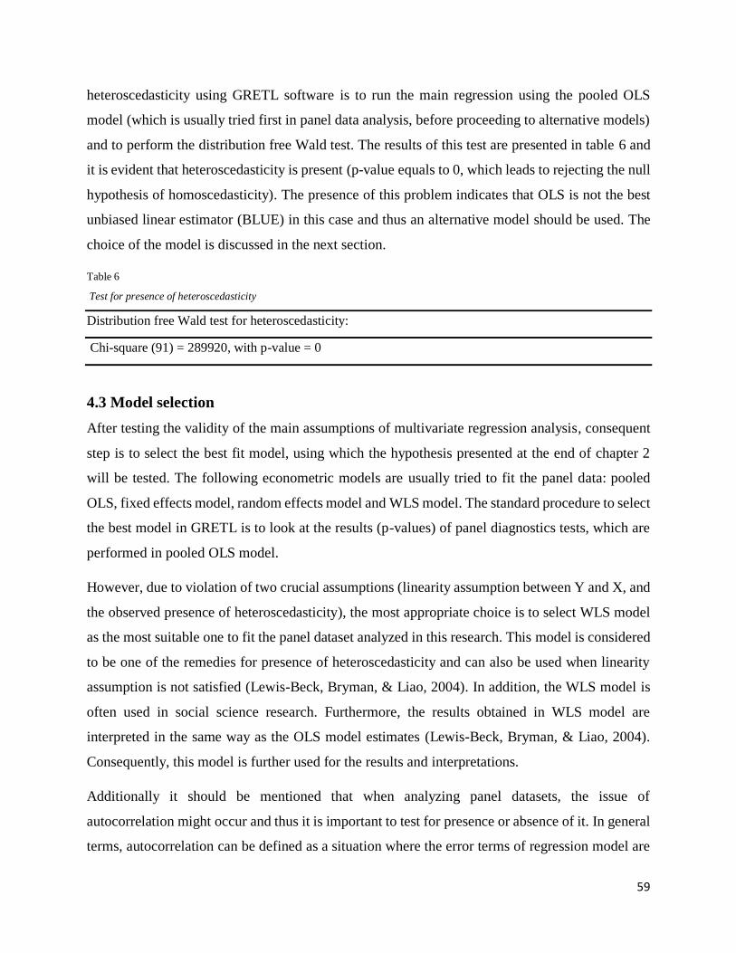
59
heteroscedasticity using GRETL software is to run the main regression using the pooled OLS
model (which is usually tried first in panel data analysis, before proceeding to alternative models)
and to perform the distribution free Wald test. The results of this test are presented in table 6 and
it is evident that heteroscedasticity is present (p-value equals to 0, which leads to rejecting the null
hypothesis of homoscedasticity). The presence of this problem indicates that OLS is not the best
unbiased linear estimator (BLUE) in this case and thus an alternative model should be used. The
choice of the model is discussed in the next section.
Table 6
Test for presence of heteroscedasticity
Distribution free Wald test for heteroscedasticity:
Chi-square (91) = 289920, with p-value = 0
4.3 Model selection
After testing the validity of the main assumptions of multivariate regression analysis, consequent
step is to select the best fit model, using which the hypothesis presented at the end of chapter 2
will be tested. The following econometric models are usually tried to fit the panel data: pooled
OLS, fixed effects model, random effects model and WLS model. The standard procedure to select
the best model in GRETL is to look at the results (p-values) of panel diagnostics tests, which are
performed in pooled OLS model.
However, due to violation of two crucial assumptions (linearity assumption between Y and X, and
the observed presence of heteroscedasticity), the most appropriate choice is to select WLS model
as the most suitable one to fit the panel dataset analyzed in this research. This model is considered
to be one of the remedies for presence of heteroscedasticity and can also be used when linearity
assumption is not satisfied (Lewis-Beck, Bryman, & Liao, 2004). In addition, the WLS model is
often used in social science research. Furthermore, the results obtained in WLS model are
interpreted in the same way as the OLS model estimates (Lewis-Beck, Bryman, & Liao, 2004).
Consequently, this model is further used for the results and interpretations.
Additionally it should be mentioned that when analyzing panel datasets, the issue of
autocorrelation might occur and thus it is important to test for presence or absence of it. In general
terms, autocorrelation can be defined as a situation where the error terms of regression model are
60
correlated over time (when using time-series data), or space (with cross-sectional data) (Lewis-
Beck, Bryman, & Liao, 2004). Presence of autocorrelation is also another indicator that OLS is
not BLUE and one of the possible solutions is considering an alternative model (e.g. WLS).
However, the WLS model is already chosen as the most suitable one due to reasons discussed
earlier in this section and its estimates also need to be checked for autocorrelation. When running
the regression using WLS model in GRETL, no additional tests need to be performed in order to
detect this issue, as the software automatically omits variables that cause autocorrelation.
Therefore, in case one or several variables are automatically omitted from the regression model,
this issue will be further discussed in the following sub-chapters.
4.4 The results
In this sub-chapter the results of panel data regression analysis are presented. The coefficients of
the variables included into the models and significance of each variables are discussed. However,
since the majority of variables were transformed for normality, rather than discussing the actual
coefficients (numbers), the directions of the effects that coefficient signs estimate (show) are
discussed instead. In the second part of this sub-chapter the robustness check is performed.
4.4.1 Model estimates
In table 7, the estimates (coefficients and significance levels) of the base model (1) and the main
model (2) with the added trade-to-GDP and development dummy interaction term are presented
(for the full model tables refer to appendix 6). As it can be noticed, both models present similar
results (in terms of coefficient signs, coefficients, and significance). However, as the estimates of
the main regression model (2) reveal, interacting trade-to-GDP and development dummy variable
does not have the expected effect on the dependent variable (GINI). The sign of the obtained
coefficient is positive, which is opposite to what was expected. However the variable is not
significant, indicating that combination of trade-to-GDP ratio and development dummy variables
does not have an effect on levels of GINI index. Consequently, trade expansion does not lead to
higher inequality levels in developing countries than in developed countries.
On the other hand, separately trade-to-GDP variable seems to be significant and having the positive
impact on the dependent variable, which also confirms the results obtained in a number of studies
reviewed in chapter 2 – increase in trade levels has inequality increasing effect. The significance
and negative sign of the estimated coefficient for the development dummy variable shows the

61
expected relationship with GINI index – more development is associated with lower levels of
income inequality.
Regarding the estimates for three remaining control variables, democracy dummy is significant,
but having an unexpected positive coefficient sign, which suggests that with more democracy,
GINI index is also expected to increase. Significant and having positive coefficient government
spending variable reveals the expected relationship – increase in this variable lowers the levels of
income inequality. Additionally, the only variable that has not been transformed for normality,
population growth rate is likewise significant and its positive coefficient indicates that higher
population growth is indeed associated with more unequal income distribution.
Finally it is important to look at the values of coefficient of determination, or the R-squared and
the adjusted R-squared. Values of this coefficient range from 0 to 1. The higher the value, the more
variation in the dependent variable is explained by the model, and the more useful the model is for
making predictions and interpretations (Weiss, 2008). Although in essence both figures are similar,
the adjusted R-squared takes into account the number of observations, sample size and the number
of independent variables included into the model (Hair, Anderson, Tatham, & Black, 1998). In this
case both values (for both the base and the main model) are very similar and rather high, which
serves as an indication that the combination of independent and control variables chosen for the
purpose of this research explains around 85% of variation of the dependent variable. However, it
is important to mention that there are several factors that might contribute to higher levels of
explained variation. These are: inclusion of a large number of independent variables into
regression, or inclusion of independent variables that are highly correlated with the dependent
variable Y (Lewis-Beck, Bryman, & Liao, 2004). Consequently, high values of R-squared and
adjusted R-squared in most cases should be interpreted cautiously.
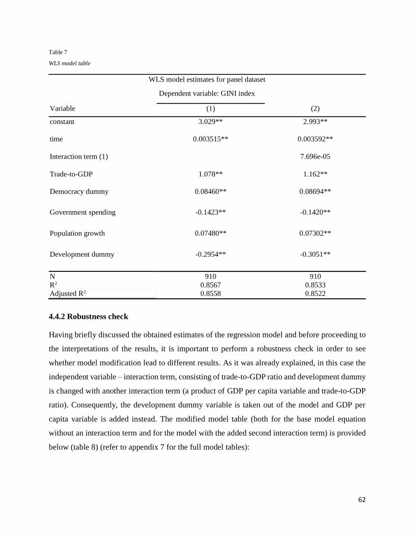
62
Table 7
WLS model table
Variable (1) (2)
constant 3.029** 2.993**
time 0.003515** 0.003592**
Interaction term (1) 7.696e-05
Trade-to-GDP 1.078** 1.162**
Democracy dummy 0.08460** 0.08694**
Government spending -0.1423** -0.1420**
Population growth 0.07480** 0.07302**
Development dummy -0.2954** -0.3051**
N
R2
910
0.8567
910
0.8533
Adjusted R2 0.8558 0.8522
4.4.2 Robustness check
Having briefly discussed the obtained estimates of the regression model and before proceeding to
the interpretations of the results, it is important to perform a robustness check in order to see
whether model modification lead to different results. As it was already explained, in this case the
independent variable – interaction term, consisting of trade-to-GDP ratio and development dummy
is changed with another interaction term (a product of GDP per capita variable and trade-to-GDP
ratio). Consequently, the development dummy variable is taken out of the model and GDP per
capita variable is added instead. The modified model table (both for the base model equation
without an interaction term and for the model with the added second interaction term) is provided
below (table 8) (refer to appendix 7 for the full model tables):
WLS model estimates for panel dataset
Dependent variable: GINI index

63
Table 8
WLS modified model table (robustness test)
Variable (3) (4)
constant 3.5931** 3.636**
time 0.0061981** 0.006081**
Interaction term (2)
−9.39768e-06
Trade-to-GDP 0.9421** 0.8374**
Democracy dummy 0.0850** 0.0864**
Government spending −0.2556** −0.2574**
Population growth 0.05622** 0.05632**
GDP per capita (log) −0.051098** −0.04992**
N
R2
910
0.7720
910
0.7690
Adjusted R2 0.7705 0.7672
As it can be seen in table 8, modifications did not significantly change the obtained results.
Although the second interaction term (interacting trade-to-GDP and GDP per capita components)
has a negative coefficient sign, it is still not significant. Thus, even when using an alternative
measure of the level of economic development, no relationship between trade-inequality effects
and the stage of development was observed.
Separately, estimates for both of the components of the second interaction are significant. Trade-
to-GDP variable has a positive coefficient sign, thus, even after modifying the model, increase in
trade-to-GDP ratio seems to be leading to more inequality. The negative coefficient sign for GDP
per capita variable indicates that in richer countries less inequality could be expected.
Identically to the previous model, all three control variables are significant and having the same
signs of estimated coefficients. The results for democracy dummy reveal the same positive effect
WLS model estimates for panel dataset
Dependent variable: GINI index

64
on GINI index, which is opposite to what was predicted. Significance and negative coefficient sign
for government spending variable again demonstrates the expected relationship to the dependent
variable – the higher government spending, the lower the inequality. Estimates for population
growth rate also confirm the previously obtained results and the theoretical expectations, as
increase in the values of this variable leads to more unequal income distribution.
Finally, the R-squared and the adjusted R-squared of the models presented in table 8 are slightly
lower than in previous models. More specifically, the estimates suggest that models presented in
table 8 explain around 77% of the variation in the dependent variable – GINI index. However, as
the levels of explained variation are high, similarly to the previous case (table 7), the estimated
values of R-squared and adjusted R-squared should be interpreted with caution due to existence of
additional factors leading to higher explained variation.
Consequently, even after modifying the regression model by adding the GDP per capita variable
as a substitute for development dummy (both separately to the model and as an interaction with
trade-to-GDP), very similar results to those presented in table 7 were obtained. This serves as a
confirmation of existent strong relationships, as even when a different measure for the level of
development is used, model estimations show almost identical results.

65
5. Interpretations and conclusions
In conclusion, this research aimed at analysing trade-inequality relationship and identifying the
possible differences in trade-inequality effects in developed and developing countries. In order to
do that, the central research question was formulated and presented in chapter 1:
What is the difference in trade effects on inequality for developing and developed countries?
In addition, 3 sub-questions were formulated. Each of the sub-questions was addressed in separate
chapters: chapter 2 aimed at answering the first sub-question by presenting the main theoretical
assumptions and existent evidence regarding trade-inequality effects and differences between
developed and developing world, which led to formulating the testable hypothesis; chapter 3
answered the second sub-question by explaining the chosen research method, presenting the
regression equation and operationalization of the variables; in chapter 4 the third research sub-
question was answered by conducting the regression analysis using panel dataset and presenting
the estimates of the final model, in addition a robustness check was performed.
This chapter aims at providing the final answer to the central research question. Therefore, after
commenting on the observed relationships in a rather technical manner in chapter 4, the results
need to be interpreted. Afterwards, based on the results and interpretations, the testable hypothesis
presented in chapter 2 is either confirmed, or rejected. In addition, this chapter discusses the
limitations of the research and provides some policy recommendations as well as suggestions for
improvements that could be made in future research on trade-inequality relationship in developing
and developed countries.
5.1 Interpretation of the results
Following the description of the final model estimates (refer to part 4.4.1), the interpretation of
these results is provided in the same sequence. Thus, starting from the independent variable
(Interaction term (1)), after conducting the panel data regression analysis, no relationship between
the combination of trade-to-GDP ratio and development dummy variable with levels of inequality
was observed. Interpretation in this case is rather straightforward: the level of country’s economic
development does not determine the effect of trade expansion on within-country income
inequality. Contrary to what was expected after conducting a literature review, trade-inequality
effects do not differ depending on how developed a country is (which group in terms of
66
development level a country belongs to), or at least this kind of relationship was not observed
during the course of this empirical research. The absence of relationship between the second
interaction term (where the variable representing trade expansion interacts with alternative
measure of the stage of development) and levels of income inequality was also confirmed by the
results of robustness test.
Consequently, the obtained estimates do not support any of the theoretical arguments presented in
chapter 2: due to absence of observed relationship, it cannot be stated that trade expansion has
inequality reducing effects in the developing world and possibly leads to higher wage gaps in
developed countries (as according to H-O and some of the convergence theorem arguments),
neither it was found that more trade does more harm in terms of levels of within-country income
inequality for the developing countries as compared to developed world (dependency theorem
argument about trade-inequality effects). Based on the obtained results and interpretations for the
independent variable of this research (combination of the state of development and trade volumes),
the testable hypothesis stating that trade expansion leads to higher income inequality in the
developing world, but not in developed countries, is rejected.
Instead, the results of this analysis are rather more general, suggesting that increase in trade
volumes is more likely to increase levels of inequality than to make the distribution of income
more egalitarian (referring to the model estimates for trade-to-GDP ratio). Although this does not
reveal anything about the possible differences in trade-inequality effects in different countries,
recalling the lack of unanimity regarding trade-inequality relationship currently existent in the
literature (chapter 2), such results then support the opinion that in general more trade has negative
consequences on income distribution. Therefore, based on the obtained estimates, the same
conclusion applies for both developed and developing world.
As for the relationship between the state of development and within-country income inequality, no
difference in terms of results obtained in the main regression model and when conducting a
robustness test was observed. When using the development dummy variable, results reveal that
more development lowers inequality. Recalling that the dummy variable has only two values
(either 0 for developing countries, or 1 for developed countries), directly interpreting the results
means stating that when a state advances and in terms of level of economic development shifts
from the category of developing countries to developed countries group, levels of within-country
67
income inequality are very likely to decrease. Regarding the alternative measure for development
– GDP per capita, results suggest that huge income gaps are more likely to be observed in poorer
countries than in rich, developed countries.
Regarding the additional factors that were added to the model based on other studies on trade-
inequality relationship, as it was already explained, the results did not change after the model was
modified. Consequently, according to the estimates, the more democratic a country is, the higher
levels of income inequality could be observed. Such results contradict the theoretical predictions
and arguments made in the studies reviewed in chapter 2, where it was stated that consolidated
democracies should demonstrate lower levels of inequality. However, regression model estimates
for the democracy dummy might be largely influenced by huge differences across the sample
countries: although majority of the countries classified as democratic and thus assigned with the
dummy value of 1 demonstrate relatively low levels of inequality throughout the time frame of
this analysis, in a number of countries, that based on the democracy score (refer to chapter 3 for
more detailed explanations about the measurement) were also assigned to the same category of
democratic states, inequality levels were much higher (Bolivia, Brazil, Honduras, India, Namibia,
Panama, Paraguay, South African Republic).
Model estimates for government spending reveal the expected relationship with income inequality
levels. More specifically, higher levels of public spending lead to lower levels of within-country
inequality. As it was explained in section 2.3, increasing levels of public spending (especially on
education and health, or social spending) is one of the ways how governments might address the
issue of income inequality and compensate those earning the lowest income, which in turn should
decrease inequality. Recalling the previously mentioned fact that developed countries have better
financial capabilities and thus are more able to compensate the poorest part of the society through
the means of public spending, this might serve as another explanation why more development
(both in terms of development dummy and GDP per capita) was found to be associated with more
egalitarian income distribution.
Finally, the results for population growth rate indicate that with higher levels of population growth,
within-country income inequality tends to increase. The observed relationship confirms the initial
expectations that population growth rate has inequality increasing effects, which was the main
reason why it was decided to take into account this factor when analyzing the trade-inequality

68
relationship (as otherwise the impact of trade expansion on within-country income inequality
might be concealed by the effects of population growth rate). In countries with rapidly increasing
population, addressing the issue of inequality might indeed be more complicated, as taking the
measures such as previously discussed compensation through public spending requires more
financial resources. Consequently, countries with high population growth rates (such as India)
demonstrate higher levels of income inequality.
5.2 Policy recommendations
Although during the course of this research no differences in trade-inequality effects in countries
on different stage of development were observed, the results revealed that separately, increase in
trade levels indeed leads to higher inequality, while more development is associated with more
equal income distribution. Therefore, trade policies in both developed and developing world
should be formulated cautiously and aimed at not only promoting trade and helping to better realize
the benefits associated with trade expansion, but also at mitigating the negative (trade-) inequality
effects. For instance, when together with rising trade volumes, increase in income inequality is
observed, certain governmental interventions, or control mechanisms could be employed.
The observed relationship between public spending and income distribution suggests that
governments could address the issue of increasing inequality by devising welfare policies aimed
at creating the so called safety nets for the most vulnerable groups in the society. Since developing
countries often lack financial resources needed to use public spending as a remedy to high
inequality levels, assistance of international organizations could be considered.
Additionally, since the results suggest that when country advances to developed country group,
income distribution becomes more egalitarian, long-term policy goal in developing world should
be aimed at primarily achieving further stage of development. Consequently, although trade
expansion would still have inequality increasing impact in more developed states, it could be
expected that more advanced countries have better capabilities to mitigate such effects, which in
turn should help reducing levels of inequality. In addition, the importance of population growth
rate has to be taken into account by countries that are involved in global trade, as this research
showed that both factors are associated with rising inequalities.
69
5.3 Limitations
One of the limitations of this research is related to the fact that the variable representing
government effectiveness had to be omitted from the model due to high multicollinearity.
Consequently, the impact of effective institutions on the level of inequality was not controlled for.
As the literature review revealed, government effectiveness could be an important factor for the
purpose of explaining the differences in trade effects in developed and developing world, as in
majority of the developing countries, institutions are rather underdeveloped. In addition, even if
this factor would have been included into the model, the chosen measurement (GE indicator)
received a lot of criticism, which to some extent indicates its low reliability. However, better
measures for institutional effectiveness are currently lacking.
Moreover, one of the reasons why depending on the level of development, no difference in trade
impact on within-country inequality was observed, might be related to the previously mentioned
limitations of dividing sample countries into two categories (developed and developing countries)
based on the World Bank’s country classification. This is relevant for the main model, where the
dummy variable is used, as when constructing it, high income countries were included into one
group, while all other countries (belonging to different categories based on the World Bank’s
classification) were assigned to the developing countries group. As a result, countries that are on
the lowest stage of economic development, and those that are in much better position, but not yet
achieved the high income category threshold, were put in the same group. Thus, even if in the
poorest countries trade expansion had the predicted effect on levels of within-country income
inequality, this might have been concealed by the opposite effects in more developed countries
within the same group. However, since during the course of this research a robustness check with
an alternative measure of development was performed and very similar results were obtained, it
can be concluded that the issue of unobserved relationships due to country categorization (using
dummy variable) was prevented.
Finally, another important limitation is data availability for developing countries. This research
aimed at including as many countries as possible into the country sample and also at having a
longer time frame, including the most recent data available. However, due to lack of available data
for the developing world, a trade-off was made, which resulted in having rather large N, but
analyzing shorter time period.

70
5.4 Implications for future research
In the future, when analyzing trade-inequality relationship and possible differences in trade impact
on inequality outcomes in developing and developed countries, several improvements could be
made: firstly with better data availability for developing countries, the time frame of the analysis
could be expanded in both directions, by analyzing even more recent data and by including several
years before 1999 (which was a starting point of this research). It is possible that having more
observations for each country would reveal some new trends that were not observed in this
research.
Secondly, with a more reliable alternative to GE index, institutional effectiveness should be
included into the analysis. The importance of government effectiveness in the context of trade-
inequality effects was emphasized in several studies reviewed in this thesis (Cornia, 2003;
Rodriguez-Pose, 2012), thus when aiming to identify differences between trade impact on wage
gap in countries on different stages of development, this has to be taken into account.
Thirdly, referring to development dummy variable, an alternative country classification could be
considered. This would allow to avoid having huge differences between the countries assigned to
the same category. Consequently, in combination with variables representing trade expansion,
using different country classification might help revealing relationships that were not observed in
this research.
Finally, since the obtained results contradicted the general argument made in the literature that
consolidated democracies have more egalitarian income distribution, an alternative measurement
for the strength of democratic regime could be used in further researches, or even different
approaches (for instance using the length of democratic regime) could be considered. Most
importantly, the fact that a number of democracies in the developing world demonstrate high levels
of inequality should certainly be taken into account.
5.5 Conclusions
In conclusion, this thesis focused on trade induced changes in inequality levels and the differences
in the effects of trade expansion on income distribution in developing and developed countries. In
addition, this research aimed at addressing the gaps currently existent in the literature analysing
trade-inequality effects. Consequently, rather than researching the impact of trade expansion on
71
income distribution in general, this thesis focused on possible differences in such effects for
developing and developed world. Accordingly, this was well reflected in theoretical and literature
review part, where the main arguments suggesting that such differences actually exist, were
presented. Additionally, the fact that previously the majority of studies on trade-inequality topic
focused mainly on developed countries was also taken into account. Therefore this research
analysed panel dataset covering a sample of 91 countries (63 developing countries and 28
developed countries) during a ten years period.
Based on the results of the regression analysis, no differences in trade effects on inequality in
countries on different stage of development were observed (regardless of the measurement used
for the level of economic development). Consequently, the hypothesis presented at the end of
chapter 2 was rejected. However, the obtained estimations indicate that separately, trade expansion
indeed increases within-country income inequality. In addition, higher stage of economic
development and more egalitarian income distribution were also found to be related. Yet, no
evidence for the combined effect of trade expansion and economic development was obtained. A
number of additional variables included into the final regression model (government spending,
population growth) were found to be having the expected impact on levels of inequality, thus
confirming the arguments made and evidence obtained by other researchers. On the other hand,
the results for democracy control variable contradicted the initial expectations. Finally, the
limitations of this research were discussed and suggestions for future improvement as well as
policy recommendations were provided.

72
References Abramovitz, M. (1986). Catching Up, Forging Ahead, and Falling Behind. The Journal of
Economic History, 46(2), 385-406.
Al-shihri, F. S. (2014). The Causal Relationship between Health and Education Expenditures in
Saudi Arabia. International Journal of Scientific and Engineering Research, 5(9), 672-
675.
Amin, S. (1972). Underdevelopment and Dependence in Black Africa - Origins and
Contemporary Forms. The Journal of Modern African Studies, 10(4), 503-524.
Anderson, E. (2005). Openness and Inequality in Developing Countries: A Review of Theory
and Recent Evidence. World Development, 33(7), 1045-1063.
Balassa, B. (1986). Dependency and Trade Orientation. The World Economy, 9(3), 259-274.
Barro, R. J. (2000). Inequality and Growth in a Panel of Countries. Journal of Economic Growth,
5(1), 5-32.
Benabou, R. (1996). Inequality and Growth. In B. S. Bernanke, & J. J. Rotemberg, NBER
Macroeconomics Annual 1996 (Vol. 11, pp. 11-92). New York: MIT Press.
Bergh, A., & Nilsson, T. (2010). Do liberalization and globalization increase income inequality?
European Journal of Political Economy, 26(4), 488-505.
Bliss, C. (2007). Trade, Growth, and Inequality. Oxford: Oxford University Press.
Bornschier, V. (1983). World Economy, Level Development and Income Distribution: An
Integration of Different Approaches to the Explanation of Income Inequality. World
Development, 11(1), 11-20.
Bussmann, M., Soysa, I. d., & Oneal, J. R. (2005). The Effect of Globalization on National
Income Inequality. Comparative Sociology, 4(3/4), 285-312.
Centre for Systematic Peace. (2016). Polity IV: Regime Authority Characteristics and
Transitions Datasets. Retrieved from Centre for Systematic Peace Web site:
http://www.systemicpeace.org/inscrdata.html
Centre for Systematic Peace. (2016). The Polity Project. Retrieved from Centre for Systematic
Peace Web site: http://www.systemicpeace.org/polityproject.html
Chilcote, R. H. (1974). Dependency Theory: A Reassessment. Latin American Perspectives,
1(1), 4-29.
Cornia, G. A. (2003). The Impact of Liberalisation and Globalisation on Income Inequality in
Developing and Transitional Economies. CESifo Working Paper No. 843.
Darity, W. A. (2008). International Encyclopedia of the Social Sciences (2nd ed.). Detroit:
Macmillan Reference USA.

73
Das, S. P. (2005). Gradual Globalization and Inequality between and within Countries. The
Canadian Journal of Economics, 38(3), 852-869.
Egger, H., & Kreickemeier, U. (2012). Fairness, trade, and inequality. Journal of International
Economics, 86(2), 184-196.
Elmawazini, K., Sharif, A., Manga, P., & Drucker, P. (2013). Trade Globalization, Financial
Globalization and Inequality Within South-East Europe and CIS Countries. The Journal
of Developing Areas, 47(2), 303-317.
Ferraro, V. (2008). Dependency Theory: An Introduction. In G. Secondi, The Development
Economics Reader (pp. 58-64). London: Routledge.
Fischer, R. D., & Serra, P. J. (1996). Income Convergence Within and Between Countries.
International Economic Review, 37(3), 531-551.
Ghose, A. K. (2001). Global economic inequality and international trade. Employment Paper
2001/12. Geneva: ILO.
Goldberg, P. K., & Pavcnik, N. (2007). Distributional Effects of Globalization in Developing
Countries. Journal of Economic Literature, 45(1), 39-82.
Hair, J. F., Anderson, R. E., Tatham, R. L., & Black, W. C. (1998). Multivariate Data Analysis
(5th ed.). New Jersey: Prentice-Hall International.
Harrison, A., McLaren, J., & McMillan, M. (2011). Recent Perspectives on Trade and Inequality.
Annual Review of Economics, 3(3), 261-289.
Helpman, E., Itskhoki, O., & Redding, S. (2010). Inequality and Unemployment in a Global
Economy. Econometrica, 78(4), 1239-1283.
Helpman, E., Itskhoki, O., Muendler, M.-A., & Redding, S. (2015). Trade and Inequality: from
theory to Estimation. Review of Economic Studies.
Hirte, G., & Lessmann, C. (2014). Trade, Integration, and Interregional Inequality. CESifo
Working Paper, No. 4799.
Jaffee, D., & Stokes, R. (1986). Foreign Investment and Trade Dependence. The Sociological
Quarterly, 27(4), 533-546.
Jaumotte, F., Lall, S., & Papageorgiou, C. (2013). Rising Income Inequality: Technology, or
Trade and Financial Globalization? IMF Economic Review, 61(2), 271-309.
Kaufmann, D., & Kraay, A. (2016). Worldwide Governance Indicators: Documentation.
Retrieved from The Worldwide Governance Indicators:
http://info.worldbank.org/governance/wgi/index.aspx#doc
Kaufmann, D., Kraay, A., & Mastruzzi, M. (2007). Worldwide Governance Indicators Project:
Answering the Critics. World Bank Policy Research Working Paper No. 4149.
74
Keeley, B. (2015). Income Inequality: The Gap between Rich and Poor. Paris: OECD
Publishing.
Kellstedt, P. M., & Whitten, G. D. (2013). The Fundamentals of Political Science Research (2nd
ed.). New York: Cambridge University Press.
Korzeniewicz, R. P., & Moran, T. P. (2009). Unveiling Inequality: A World - Historical
Perspective. New York: Russell Sage Foundation.
Lee, E., & Vivarelli, M. (2006). The Social Impact of Globalization in the Developing Countries.
International Labour Review, 145(3), 167-184.
Lewis-Beck, M. S., Bryman, A., & Liao, T. F. (2004). The SAGE Encyclopedia of Social Science
Research Methods. Thousand Oaks: Sage Publications.
Liberati, P. (2015). The World Distribution of Income and it's Inequality, 1970-2009. Review of
Income and Wealth, 61(2), 248-273.
Lin, P. C., & Huang, H. C. (2011). Inequality convergence in a panel of states. The Journal of
Economic Inequality, 9(2), 195-206.
Mahler, V. A., Jesuit, D. K., & Roscoe, D. D. (1999). Exploring the Impact of Trade and
Investment on Income Inequality. Comparative Political Studies, 32(3), 363-395.
Mayer-Foulkes, D. (2002). Global Divergence. Mexico: Centro de Investigación y Docencia
Económicas (CIDE) - Division of Economics.
Matano, A., & Naticchioni, P. (2010). Trade and Wage Inequality: Local versus Global
Comparative Advantages. The World Economy, 33(2), 1757-1787.
Meschi, E., & Vivarelli, M. (2008). Trade and Income Inequality in Developing Countries.
World Development, 37(2), 287-302.
Milanovic, B. (2005). Worlds Apart: Global and International Inequality, 1950-2000. Princeton,
NJ: Princeton University Press.
Milanovic, B. (2006). Global Income Inequality: What It Is And Why It Matters? World
Economics, 7(1), 131-157.
Milanovic, B., & Squire, L. (2005). Does Tariff Liberalization Increase Wage Inequality? Some
Empirical Evidence. World Bank Policy Research Working Paper No. 3571(11046).
Washington, DC: The World Bank.
OECD. (2015). In It Together: Why Less Inequality Benefits All. Paris: OECD Publishing.
O'Rourke, K. H. (2001). Globalization and Inequality: Historical Trends. Cambridge, MA:
National Bureau of Economic Research.
Pfaffenberger, R. C., & Patterson, J. H. (1987). Statistical Methods for Business and Economics
(3rd ed.). Homewood, IL: Irwin McGraw-Hil.
75
Punch, K. F. (1998). Introduction to Social Research. Quantitative and Qualitative Approaches.
London/Thousand Oaks/New Delhi: Sage.
Rahman, M. M. (2011). Causal Relationship among Education Expenditure, Health Expenditure
and GDP: A Case Study for Bangladesh. International Journal of Economics and
Finance, 3(3), 149-159.
Ravallion, M. (2001). Growth, Inequality and Poverty: Looking Beyond Averages. World
Development, 29(11), 1803-1815.
Reuveny, R., & Li, Q. (2003). Economic Openness, Democracy, and Income Inequality. An
Empirical Analysis. Comparative Political Studies, 36(5), 575-601.
Rodriguez-Pose, A. (2012). Trade and Regional Inequality. Economic Geogprahy, 88(2), 109-
136.
Rudra, N. (2004). Openness, Welfare Spending, and Inequality in the Developing World.
International Studies Quarterly, 48(3), 683-709.
Sala-i-Martin, X. (2002). The World Distribution of Income (Estimated from Individual Country
Distribution). Cambridge, MA: National Bureau of Economic Research.
Solt, F. (2009). The Standardized World Income Inequality Database. Harvard Dataverse.
Retrieved from http://hdl.handle.net/1902.1/11992
The World Bank . (n.d.). Data: Trade (% of GDP). Retrieved from World Development
Indicators: http://data.worldbank.org/indicator/NE.TRD.GNFS.ZS
The World Bank. (2007). Global Economic Prospects: Managing the Next Wave of
Globalization. Washington DC: The World Bank.
The World Bank. (2016). Countries and Lending Groups. Retrieved from The World Bank Data
site: http://data.worldbank.org/about/country-and-lending-groups
The World Bank. (n.d.). Data: GDP per capita. Retrieved from World Development Indicators:
http://data.worldbank.org/indicator/NY.GDP.PCAP.CD/countries
The World Bank. (n.d.). Data: Health expenditure, total (% GDP). Retrieved from World
Development Indicators: http://data.worldbank.org/indicator/SH.XPD.TOTL.ZS
The World Bank. (n.d.). Data: population growth (% annual). Retrieved from World
Development Indicators: http://data.worldbank.org/indicator/SP.POP.GROW
Trochim, W. M. (2000). The Research Methods Knowledge Base, 2nd Edition. Cincinnati:
Atomic Dog Publishing.
Uoardighi, J. E., & Somun-Kapetanovic, R. (2009). Convergence and Inequality of income: the
case of Werstern Balkan countries. The European Journal of Comparative Economics,
6(2), 207-225.

76
Weiss, N. A. (2008). Elementary Statistics (7th ed.). Boston: Pearson Education.
Winters, L. A., McCulloch, N., & McKay, A. (2004). Trade Liberalization and Poverty: The
Evidence So Far. Journal of Economic Literature, 42(1), 72-115.
World Trade Organization. (2008). World trade report 2008: Trade in a Globalizing World.
Geneva: World Trade Organization.

77
Appendices
Appendix 1
Country sample
Argentina Indonesia Peru
Armenia Iran Philippines
Australia Ireland Poland
Austria Israel Portugal
Bangladesh Italy Romania
Belarus Japan Russia
Belgium Jordan Rwanda
Bolivia Kazakhstan Senegal
Brazil Korea Sierra Leone
Canada Kyrgyz Republic Singapore
Chile Latvia Slovak Republic
China Lithuania Slovenia
Colombia Luxembourg South African Republic
Costa Rica Macedonia Spain
Croatia Madagascar Sri Lanka
Cyprus Malawi Sweden
Czech Republic Malaysia Switzerland
Denmark Mali Tanzania
Dominican Republic Mexico Thailand
Ecuador Moldova Tunisia
El Salvador Mongolia Turkey
Estonia Namibia Uganda
Finland Nepal Ukraine
France Netherlands United Kingdom
Georgia New Zealand United States
Germany Nigeria Uruguay
Greece Norway Venezuela
Guatemala Pakistan Vietnam
Honduras Panama Zambia
Hungary Paraguay Zimbabwe
India
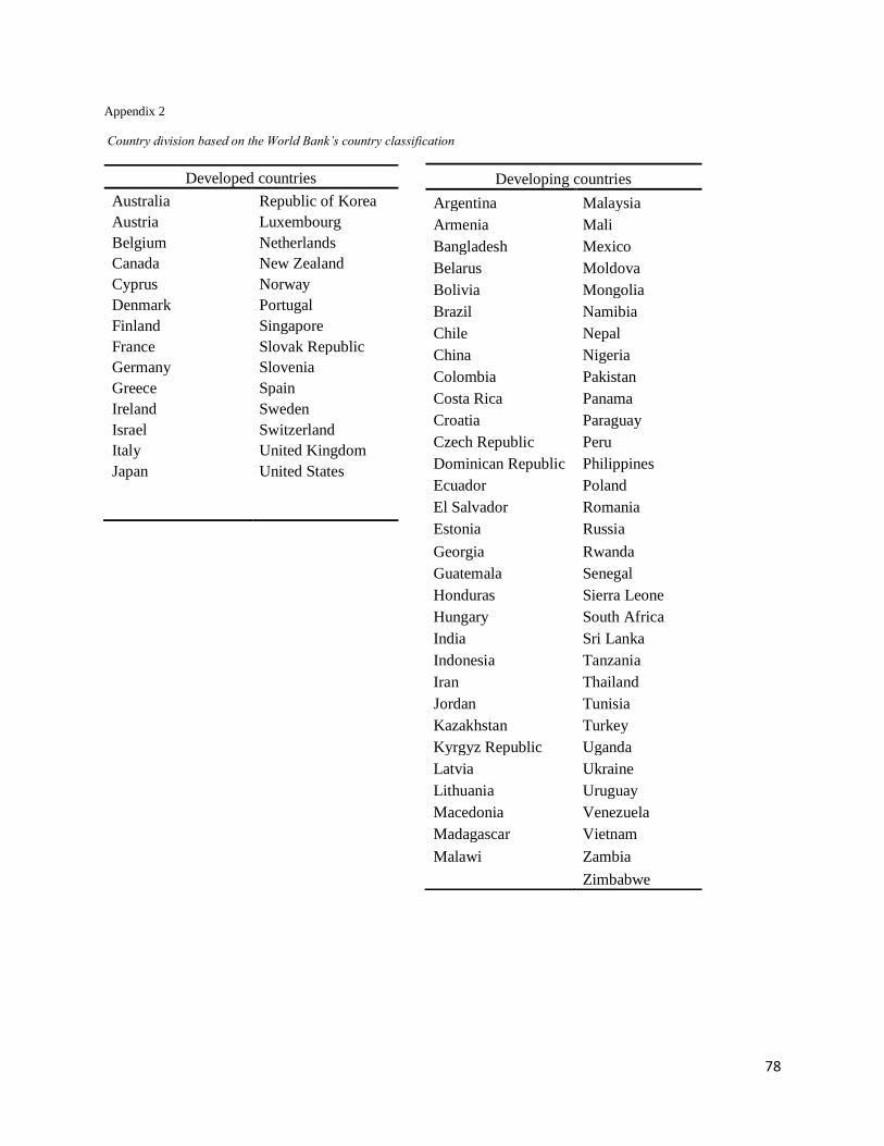
78
Appendix 2
Country division based on the World Bank’s country classification
Developed countries
Australia Republic of Korea
Austria Luxembourg
Belgium Netherlands
Canada New Zealand
Cyprus Norway
Denmark Portugal
Finland Singapore
France Slovak Republic
Germany Slovenia
Greece Spain
Ireland Sweden
Israel Switzerland
Italy United Kingdom
Japan United States
Developing countries
Argentina Malaysia
Armenia Mali
Bangladesh Mexico
Belarus Moldova
Bolivia Mongolia
Brazil Namibia
Chile Nepal
China Nigeria
Colombia Pakistan
Costa Rica Panama
Croatia Paraguay
Czech Republic Peru
Dominican Republic Philippines
Ecuador Poland
El Salvador Romania
Estonia Russia
Georgia Rwanda
Guatemala Senegal
Honduras Sierra Leone
Hungary South Africa
India Sri Lanka
Indonesia Tanzania
Iran Thailand
Jordan Tunisia
Kazakhstan Turkey
Kyrgyz Republic Uganda
Latvia Ukraine
Lithuania Uruguay
Macedonia Venezuela
Madagascar Vietnam
Malawi Zambia
Zimbabwe

79
Appendix 3
Normality tests
a) Frequency distribution for the original government effectiveness variable
b) Frequency distribution for the transformed government effectiveness variable (using exponent (-1/5))
0
0,1
0,2
0,3
0,4
0,5
0,6
0,7
-2 -1 0 1 2 3
Densi
ty
GE
GE
N(0,33757 0,98661)Test statistic for normality:
Chi-square(2) = 178,850 [0,0000]
0
1
2
3
4
5
6
7
8
9
0,65 0,7 0,75 0,8 0,85 0,9 0,95 1
Density
GE_trans
GE_trans
N(0,82382 0,058385)Test statistic for normality:
Chi-square(2) = 46,445 [0,0000]
Mean 0.34 Median 0.11
Skewness 0.40
Kurtosis -1.10
Mean 0.82
Median 0.83
Skewness 0.17
Kurtosis -0.81

80
c) Frequency distribution for the original government spending variable
d) Frequency distribution for the transformed government spending variable (using exponent (1/3))
0
0,05
0,1
0,15
0,2
0,25
-2 0 2 4 6 8 10
Density
GOVS
GOVS
N(3,9565 2,007)Test statistic for normality:
Chi-square(2) = 99,404 [0,0000]
0
0,2
0,4
0,6
0,8
1
1,2
1,4
0,6 0,8 1 1,2 1,4 1,6 1,8 2 2,2 2,4
Density
GOVS_trans
GOVS_trans
N(1,5306 0,28677)Test statistic for normality:
Chi-square(2) = 60,160 [0,0000]
Mean 3.96 Median 3.68
Skewness 0.33
Kurtosis -0.91
Mean 1.53 Median 1.54
Skewness -0.26
Kurtosis -0.79
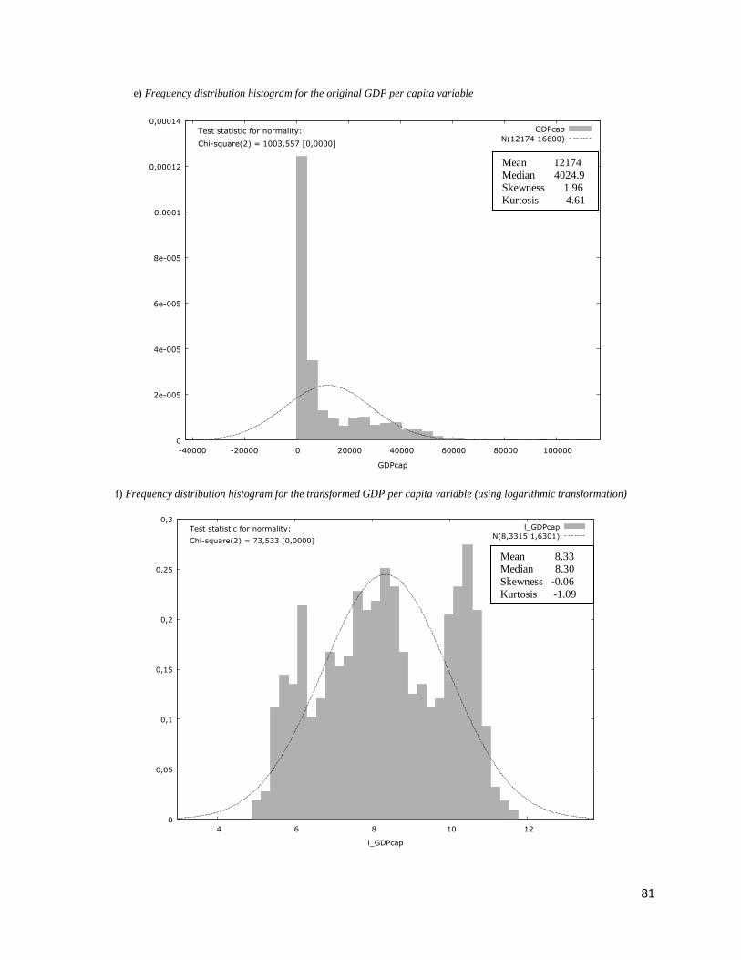
81
e) Frequency distribution histogram for the original GDP per capita variable
f) Frequency distribution histogram for the transformed GDP per capita variable (using logarithmic transformation)
0
2e-005
4e-005
6e-005
8e-005
0,0001
0,00012
0,00014
-40000 -20000 0 20000 40000 60000 80000 100000
Density
GDPcap
GDPcap
N(12174 16600)Test statistic for normality:
Chi-square(2) = 1003,557 [0,0000]
0
0,05
0,1
0,15
0,2
0,25
0,3
4 6 8 10 12
Density
l_GDPcap
l_GDPcap
N(8,3315 1,6301)Test statistic for normality:
Chi-square(2) = 73,533 [0,0000]
Mean 12174
Median 4024.9
Skewness 1.96
Kurtosis 4.61
Mean 8.33 Median 8.30
Skewness -0.06
Kurtosis -1.09

82
g) Frequency distribution for the original democracy variable
h) Frequency distribution for the original population growth variable
0
0,05
0,1
0,15
0,2
0,25
0,3
0,35
-5 0 5 10 15 20
Density
DEM
DEM
N(6,2824 4,8975)Test statistic for normality:
Chi-square(2) = 1374,930 [0,0000]
0
0,05
0,1
0,15
0,2
0,25
0,3
0,35
0,4
0,45
-2 0 2 4 6
Density
Pgrowth
Pgrowth
N(1,0703 1,1201)Test statistic for normality:
Chi-square(2) = 45,180 [0,0000]
Mean 6.28
Median 8.00
Skewness -1.54
Kurtosis 1.16
Mean 1.07
Median 1.12 Skewness 0.36
Kurtosis 1.32

83
Appendix 4
Summary of transformations for normality
ORIGINAL VARIABLE TRANSFORMED VARIABLE
Variable Test 12 Test 23 Test 34 Test 45 Transformation Test 1 Test 2 Test 3 Test 4
Democracy 2.74E-299 1.6253E-35 0 5.20602E-90 Dummy introduced
- - - -
Gov. effectiveness 1.4562E-39 1.1698E-19 0 8.1851E-16 GE^(-1/5) 8.2134E-11 1.0758E-14 0 3.763E-07
Gov. spending 2.5983E-22 2.6471E-14 0 4.6009E-11 GOVS^(1/3) 8.6397E-14 5.0087E-11 0 44923E-08
GDP per capita 1.203E-218 6.0762E-36 0 1.638E-302 GDPcap(log) 1.0779E-16 2.6782E-14 0 1.4351E-10
Population growth 1.5466E-10 4.025E-07 0,01 2.63257E-19 No transformation - - - -
2 Results of Doornik-Hansen test conducted in GRETL 3 Results of Shapiro-Wilk W test conducted in GRETL 4 Results of Lilliefors test conducted in GRETL 5 Results of Jarque-Bera test conducted in GRETL

84
Appendix 5
Scatter plots for linearity
GIN
I_tr
ans
TGDP_trans
GIN
I_tr
ans
GE_trans
GIN
I_tr
ans
GOVS_trans
GIN
I_tr
ans
Pgrowth
GIN
I_tr
ans
l_GDPcap
GIN
I_tr
ans
INTER2

85
Appendix 6
Full model tables
a) Base model
Base model: WLS
Dependent variable: GINI index
Variables Coefficient Std. Error t-ratio p-value
constant 3.02871 0.0356537 84.9478 <0.0001 ***
time 0.00351504 0.00096871 3.6286 0.0003 ***
Trade-to-GDP 1.07818 0.0670712 16.0751 <0.0001 ***
Democracy dummy 0.0846049 0.00845086 10.0114 <0.0001 ***
Government spending −0.142306 0.0146107 −9.7398 <0.0001 ***
Population growth 0.0748018 0.0029773 25.1240 <0.0001 ***
Development dummy −0.295395 0.00818939 −36.0704 <0.0001 ***
R-squared 0.856791 Adjusted R-squared 0.855840
b) Main model
Main model: WLS
Dependent variable: GINI index
Variables Coefficient Std. Error t-ratio p-value
constant 2.99285 0.0450295 66.4643 <0.0001 ***
time 0.00359157 0.000987656 3.6365 0.0003 ***
Interaction term (1) 7.69621e-05 0.000123781 0.6218 0.5343
Trade-to-GDP 1.16151 0.0922254 12.5942 <0.0001 ***
Democracy dummy 0.0869395 0.00863873 10.0639 <0.0001 ***
Government spending −0.14201 0.0151371 −9.3816 <0.0001 ***
Population growth 0.0730247 0.00312494 23.3683 <0.0001 ***
Development dummy −0.305101 0.0133438 −22.8647 <0.0001 ***
R-squared 0.853317 Adjusted R-squared 0.852179

86
Appendix 7
Robustness check
a) Base model for robustness check
Model: WLS
Dependent variable: GINI index
Variables Coefficient Std. Error t-ratio p-value
constant 3.59305 0.0404094 88.9161 <0.0001 ***
time 0.00619806 0.000893101 6.9399 <0.0001 ***
Trade-to-GDP 0.942109 0.0795295 11.8460 <0.0001 ***
Democracy dummy 0.0850241 0.0101441 8.3817 <0.0001 ***
Government spending −0.255559 0.0197254 −12.9558 <0.0001 ***
Population growth 0.0562172 0.00324458 17.3265 <0.0001 ***
GDP per capita (log) −0.0510983 0.00383875 −13.3112 <0.0001 ***
R-squared 0.772048 Adjusted R-squared 0.770533
b) Main model for robustness check
Model: WLS
Dependent variable: GINI index
Variables Coefficient Std. Error t-ratio p-value
constant 3.63555 0.0707025 51.4204 <0.0001 ***
time 0.00608089 0.000896513 6.7828 <0.0001 ***
Interaction term (2) −9.39768e-06 1.41451e-05 −0.6644 0.5066
Trade-to-GDP 0.837418 0.159037 5.2656 <0.0001 ***
Democracy dummy 0.086418 0.0101679 8.4991 <0.0001 ***
Government spending −0.257358 0.0202311 −12.7209 <0.0001 ***
Population growth 0.0563162 0.00329462 17.0934 <0.0001 ***
GDP per capita (log) −0.0499183 0.00433811 −11.5069 <0.0001 ***
R-squared 0.768971 Adjusted R-squared 0.767178
Top Related