


Languages
Pages
Legal

The impact of minimum legal drinking age laws on alcohol consumption, smoking, and marijuana use: Evidence from a regression
discontinuity design using exact date of birth
Barış K. Yörük† University at Albany, SUNY
Ceren Ertan Yörük‡ Northeastern University
Abstract
This paper uses a regression discontinuity design to estimate the impact of the minimum legal drinking age laws on alcohol consumption, smoking, and marijuana use among young adults. Using data from the National Longitudinal Survey of Youth (1997 Cohort), we find that granting legal access to alcohol at age 21 leads to an increase in several measures of alcohol consumption, including an up to a 10 percentage point increase in the probability of drinking. Furthermore, this effect is robust under several different parametric and non-parametric models. We also find some evidence that the discrete jump in alcohol consumption at age 21 has negative spillover effects on marijuana use but does not affect the smoking habits of young adults. Our results indicate that although the change in alcohol consumption habits of young adults following their 21st birthday is less severe than previously known, policies that are designed to reduce drinking among young adults may have desirable impacts and can create public health benefits. Keywords: alcohol consumption, marijuana use, minimum legal drinking age, smoking JEL classification: I10, I18, I19 † Corresponding author. Department of Economics, University at Albany, SUNY. E-mail: [email protected] ‡ Department of Economics, Northeastern University. E-mail: [email protected]
The impact of minimum legal drinking age laws on alcohol
consumption, smoking, and marijuana use: Evidence from a
regression discontinuity design using exact date of birth
January 24, 2011
Abstract
This paper uses a regression discontinuity design to estimate the impact of the minimum legal
drinking age laws on alcohol consumption, smoking, and marijuana use among young adults.
Using data from the National Longitudinal Survey of Youth (1997 Cohort), we find that granting
legal access to alcohol at age 21 leads to an increase in several measures of alcohol consumption,
including an up to a 10 percentage point increase in the probability of drinking. Furthermore, this
effect is robust under several different parametric and non-parametric models. We also find some
evidence that the discrete jump in alcohol consumption at age 21 has negative spillover effects on
marijuana use but does not affect the smoking habits of young adults. Our results indicate that
although the change in alcohol consumption habits of young adults following their 21st birthday
is less severe than previously known, policies that are designed to reduce drinking among young
adults may have desirable impacts and can create public health benefits.
Keywords: alcohol consumption, marijuana use, minimum legal drinking age, smoking
JEL classification: I10, I18, I19
1 Introduction
While consuming alcohol sensibly is generally associated with better health and longer life, the abuse
of alcohol is associated with many undesirable health outcomes. For instance, several studies link
heavy alcohol consumption with low blood pressure, increased risk of stroke, liver diseases, and
1
kidney failure.1 Furthermore, the benefits of moderate drinking are found to be mostly small, while
the damage caused by heavy drinking appears to be considerable.2 A large body of literature also
documents considerable spillover effects of alcohol consumption on labor market outcomes, risky
behavior, alcohol related traffic injuries and fatalities, and criminal activity.3 Given these direct and
indirect effects of alcohol use, evaluating the effectiveness of the policies regulating alcohol availability
and consumption is vital.
Many studies have shown that policies that increase the full cost of consuming alcohol such
as restricting the days of alcohol sales, toughening drunk driving laws, and raising alcohol taxes
significantly decrease alcohol consumption and have positive spillover effects on alcohol consumption
related outcomes. One of the most direct forms of regulation on alcohol availability in the United
States is imposing a minimum legal drinking age (hereafter, MLDA) of 21. Understanding the effect
of the MLDA is particularly important not only because alcohol consumption is related to several
undesirable health and economic outcomes, but also lowering the MLDA from 21 is a current policy
debate in many states. Proponents of the MLDA of 21 argue that imposing an age limit encourages
a majority of young adults under age 21 to consume alcohol in an irresponsible manner and that
lowering the drinking age would help young adults to learn how to drink gradually, safely and in
moderation. However, opponents of lowering the drinking age argue that states that previously
lowered the drinking age to 18, such as Massachusetts, Michigan, and Maine, experienced an increase
in alcohol-related traffic accidents among the 18 to 20 age group.
Although several studies have investigated the effect of the MLDA laws on alcohol consumption,
most of them have made use of the changes in the MLDA that occurred in the 1970s and 1980s at the
state level. However, states where a lower MLDA was imposed might be different in unobserved ways
than those states where the MLDA of 21 was enforced. If these unobserved differences at the state
level are also associated with drinking habits of young adults, than one cannot estimate a consistent
effect of the MLDA on alcohol consumption and alcohol consumption related outcomes using the
simple variation of the MLDA law at the state level. In order to address this shortcoming, we exploit
the discontinuity in drinking habits of young adults at age 21 and use a regression discontinuity
1See, for example, Hansagi et al. (1995), Mann, Smart, and Govoni (2003), and Niholson and Taylor (1940).2Poikolainen (1996) discusses the relationship between alcohol consumption and overall health outcomes in detail.3According to the recent National Highway Safety Administration data, in 2008, 37 percent of traffic fatalities in the
United States were alcohol related. In recent papers, Carpenter and Dobkin (2008) and Markowitz (2005) document
the relationship between alcohol consumption and crime.
2
(hereafter, RD) design to estimate the causal effect of the MLDA on alcohol consumption, smoking,
and marijuana use among young adults. Our main identifying assumption is that the observed and
unobserved determinants of these outcomes are likely to be distributed smoothly across the age-21
cutoff.4 Hence, the changes in alcohol consumption, smoking, and marijuana use trends at age 21
can solely be attributed to the MLDA law itself.
We use a restricted version of the National Longitudinal Survey of Youth, 1997 Cohort (NLSY97)
for the empirical analysis, which contains a unique information on the exact birth dates of the respon-
dents. In the context of a RD design, this unique information is particularly important since one can
clearly identify the treatment and control groups and compare the drinking, smoking, and marijuana
use habits of young adults who are just about to turn 21 with those who recently turned 21.5
This paper makes two main contribution to the existing literature. First, using a restricted version
of NLSY97, our study provides new estimates of the effect of the MLDA on alcohol consumption
behavior of young adults. Similar to the previous studies, our results suggest that granting legal
access to alcohol at age 21 leads to an increase in several measures of alcohol consumption. In
particular, we find that the MLDA of 21 is associated with up to a 10 percentage point increase in
the probability of alcohol consumption and a more than 1.7 day increase in the number of days that
young adults consume alcohol per month. We also document that the MLDA increases the probability
of binge drinking up to 8 percentage points under different parametric specifications. However, in
contrast to previous literature, we find that MLDA does not significantly effect the number of drinks
that young adults had on the days they consumed alcohol. Furthermore, the MLDA increases youths’
average alcohol consumption per day by only 0.2 drinks under certain specifications, which suggests
that the effect of the MLDA on drinking habits of young adults is less severe than previously known.
Second, we investigate the relationship between alcohol consumption and two alcohol consumption
related outcomes, namely smoking and marijuana use. The existing literature provides mixed results
for the possible relationship between alcohol consumption and these two alcohol related outcomes.
4This assumption is partially testable. We present the relevant tests in section 5.5Suppose that one has information only on the month and year of the birthdate of each respondent and her interview
date. Then, treatment and control groups cannot be cleary identified. For instance, a respondent who was born on
January 30, 1980 and interviewed on January 1, 2001 will be mistakenly coded as a 21 year old and placed in a treatment
group (those who are 21 and older). But, this respondent is actually in the control group since she is 29 days younger
than 21 at the time of the interview. Furthermore, by definition, the RD approach estimates the local treatment effect,
which calls for a very detailed information around the age-21 cutoff.
3
We find some evidence that the discrete jump in alcohol consumption at age 21 has negative spillover
effects on marijuana use. In particular, our results imply that under certain specifications, the proba-
bility of marijuana use among young adults tend to increase up to 7 percentage points at age-21 cutoff.
However, we find no significant effect of the MLDA on smoking habits of young adults. Furthermore,
in general, these results are robust under several parametric or non-parametric specifications.
The rest of this paper is organized as follows. The next section provides a summary of the history
of the MLDA laws in the United States and discusses the relevant research. Section three presents
the data and discusses the relationship between the MLDA and alcohol consumption, marijuana use,
and smoking. Section four sets out the specifications for different empirical models. Section five
presents the results and discusses the robustness of the main findings. Section six interprets the
results, provides a discussion of policy implications, and concludes.
2 Background and literature review
For almost 40 years, most states voluntarily set their minimum drinking age law at 21. However,
starting from early 1970s, several states began lowering their drinking age.6 As the issue of drunk
driving became more pronounced and was linked with traffic fatalities and injuries, by 1983, most
of the states raised their drinking age back to 21. On July 17, 1984, President Reagan signed into
law the National Uniform Drinking Age Act mandating all states to adopt 21 as the legal drinking
age within five years.7 By 1988, all states had set 21 as the minimum drinking age. Since then, it is
illegal for youths under age 21 to purchase or consume alcohol in the United States.8
There is extensive literature which investigates the effect of the MLDA laws on alcohol consump-
tion and alcohol consumption related outcomes.9 Most of the earlier studies used the state level
variation in the MLDA laws before 1988 to identify the effect of these laws on alcohol consumption.
For instance, Carpenter et al. (2007) provide a historical comparative analysis of the effect of the
6Among these states, there was no uniformity in age limits. The drinking ages varied from 18 to 20 and sometimes
varied based on the type of the alcohol being consumed.7States that did not comply faced a reduction in highway funds under the Federal Highway Aid Act.8 In some states, alcohol consumption under 21 may be allowed for religious or educational purposes or if a parent is
present. We do not address these exceptions directly because their impact is likely to be fairly minor in the context of
our study.9Most of these studies focus on the effect of the MLDA laws on alcohol related traffic injuries and fatalities. See, for
example, Lovenheim and Slemrod (2010), Carpenter and Dobkin (2009), and Kreft and Epling 2007). Wagenaar and
Toomey (2002) provide an extensive review of the literature on the effects of minimum drinking age laws.
4
MLDA laws on drinking behavior of high school seniors. They find that nationwide increases in the
MLDA in the late 1970s and 1980s significantly reduced alcohol consumption by high school seniors.
Dee and Evans (2003) argue that teens who faced a lower MLDA were substantially more likely to
drink. However, changes in the MLDA had small and statistically insignificant effects on educational
attainment. Laixuthai and Chaloupka (1993) examine the frequencies of youth drinking and heavy
drinking and the effects of the MLDA and beer excise taxes for 1982 and 1989. They find that in
both years, drinking is responsive to price changes resulting from higher excise taxes. However, the
price sensitivity of youth alcohol use fell after states changed to a uniform MLDA of 21. On the other
hand, Miron and Tetelbaum (2009) use state level panel data to show that any nationwide impact of
the MLDA is driven by states that increased their MLDA prior to any inducement from the federal
government. They argue that even in early-adopting states, the impact of the MLDA did not persist
much past the year of adoption and the MLDA appears to have only a minor impact on teen drinking.
The main concern in identifying the relationship between the MLDA and alcohol consumption is
the possibility that some unobserved characteristics that are correlated with drinking behavior such
as state level alcohol consumption trends may also be associated with the MLDA law itself. Although
using the variation in the MLDA before 1988 at the state level partially addresses this problem, the
states that enforced a lower MLDA might be different in unobserved ways than those states that
enforced the MLDA of 21. If these unobserved differences at the state level are also correlated with
drinking behavior, than one cannot directly estimate a consistent effect of the MLDA on alcohol
consumption using the simple variation of the MLDA law at the state level. The RD approach used
in this paper alleviates this shortcoming by removing the bias from unobserved policy preferences.
Our approach follows that of Carpenter and Dobkin (2009) who investigate the effect of the MLDA
on alcohol consumption and alcohol consumption related mortalities using the RD design. They find
that granting legal access to alcohol at age 21 leads to large increases in several measures of alcohol
consumption, including a 21 percent increase in the number of days on which people drink. This
increase in alcohol consumption results in a discrete 9 percent increase in the mortality rate at age
21. However, our study differs from that of Carperter and Dobkin in several ways. First, we employ
a different individual level survey (NLSY97) that contains information on the exact birth day of
the respondents. The NLSY97 has also the advantage of containing a more comprehensive range of
alcohol consumption and alcohol consumption related outcomes than previous research.
5
Several studies also analyze the relationship between alcohol consumption and smoking and mar-
ijuana use among young adults. The results are mixed. For example, DiNardo and Lemieux (2001)
find that increases in the MLDA did reduce the prevalence of alcohol consumption. However, in-
creased MLDAs during the 1980-1989 had the unintended consequence of increasing the prevalence of
marijuana consumption among young adults. Chaloupka and Laixuthai (1997) examine the substi-
tutability of alcoholic beverages and marijuana among youths. They use beer prices and the variation
in the MLDA at the state level as measures of the full price of alcohol and an indicator of marijuana
decriminalization and its money price as the full price of marijuana. They find that drinking fre-
quency and heavy drinking episodes are negatively related to beer prices, but positively related to
the full price of marijuana. However, Pacula (1998) argues that alcohol and marijuana are economic
complements, not substitutes and that increases in the federal tax on beer will generate a larger
reduction in the unconditional demand for marijuana than for alcohol in percentage terms.
Dee (1999) investigates the relationship between alcohol consumption and smoking. He finds that
the movement away from minimum legal drinking ages of 18 reduced teen smoking participation by
3 to 5 percent. Furthermore, his corresponding instrumental variable estimates suggest that teen
drinking roughly doubles the mean probability of smoking participation. On the other hand, Goel
and Morey (1995) find that own-price elasticity of cigarettes is greater than that of liquor suggesting
that liquor consumption is less responsive to its own price changes than is cigarette consumption and
that these two goods are substitutes in consumption. Our paper provides new estimates of the effect
of alcohol consumption on marijuana use and smoking among young adults using a different empirical
approach and a unique data that enables one to clearly identify the treatment and control groups.
3 Data
In this paper, we use data from the NLSY97 for the empirical analysis. The NLSY97 consists of a
nationally representative sample of approximately 9,000 youths who were 12 to 16 years old as of
December 31, 1996. Round 1 of the survey took place in 1997. In that round, both the eligible youth
and one of that youth’s parents received hour-long personal interviews. Youths continue to be inter-
viewed on an annual basis. In addition to standard demographic information, the survey respondents
were asked about their drinking, smoking, and drug use habits. We present the description of key
6
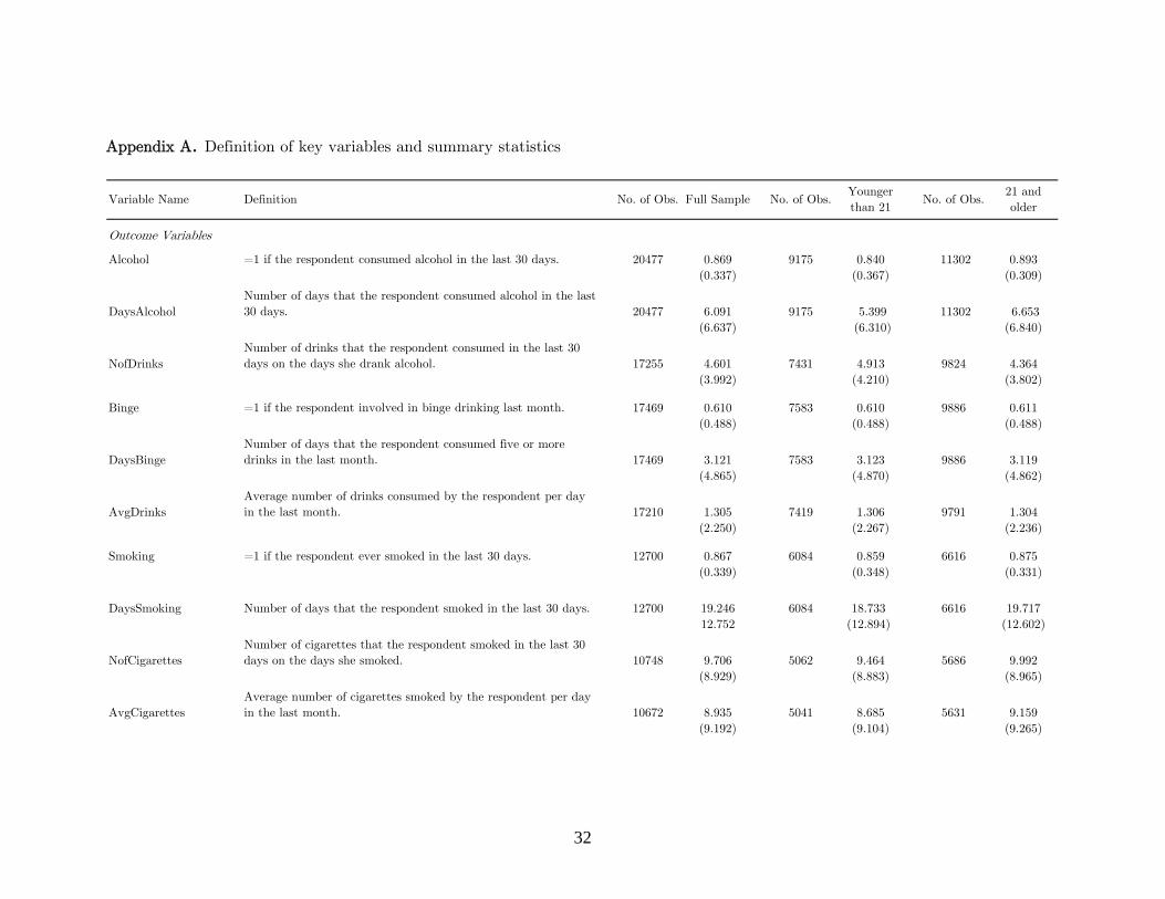
variables used in the empirical analysis and their summary statistics in Appendix A.
A unique feature of our data set is that we have obtained access to a confidential version of the
NLSY97 with information on respondents’ exact date of birth and exact interview date for each survey
year. We use this information to calculate the exact age in days for each respondent at the time of the
interview. We restrict our sample to those respondents who were surveyed over the period 2000-2006
and were between ages 19 to 22, inclusive.10
In contrast to similar surveys of its kind, the respondents of the NLSY97 were asked about their
alcohol consumption habits over the past month.11 This relatively short reference period is desirable
since our empirical strategy compares those who are slightly older than 21 with those who are slightly
younger than this cutoff age. In general, we consider six main alcohol consumption outcomes. Two
of these outcomes are measures of drinking participation, i.e., whether the respondent consumed
alcohol over the past month and whether the respondent engaged in heavy (binge) drinking in the
past month.12 Two of the remaining variables measure the number of days that the respondent had at
least one drink and the number of days that she had five or more drinks on the same occasion during
the past month. Finally, the remaining two outcome variables measure the intensity of drinking as
the average number of drinks that the respondent had on the days she consumed alcohol and average
number of drinks that she had per day during a one month period.13
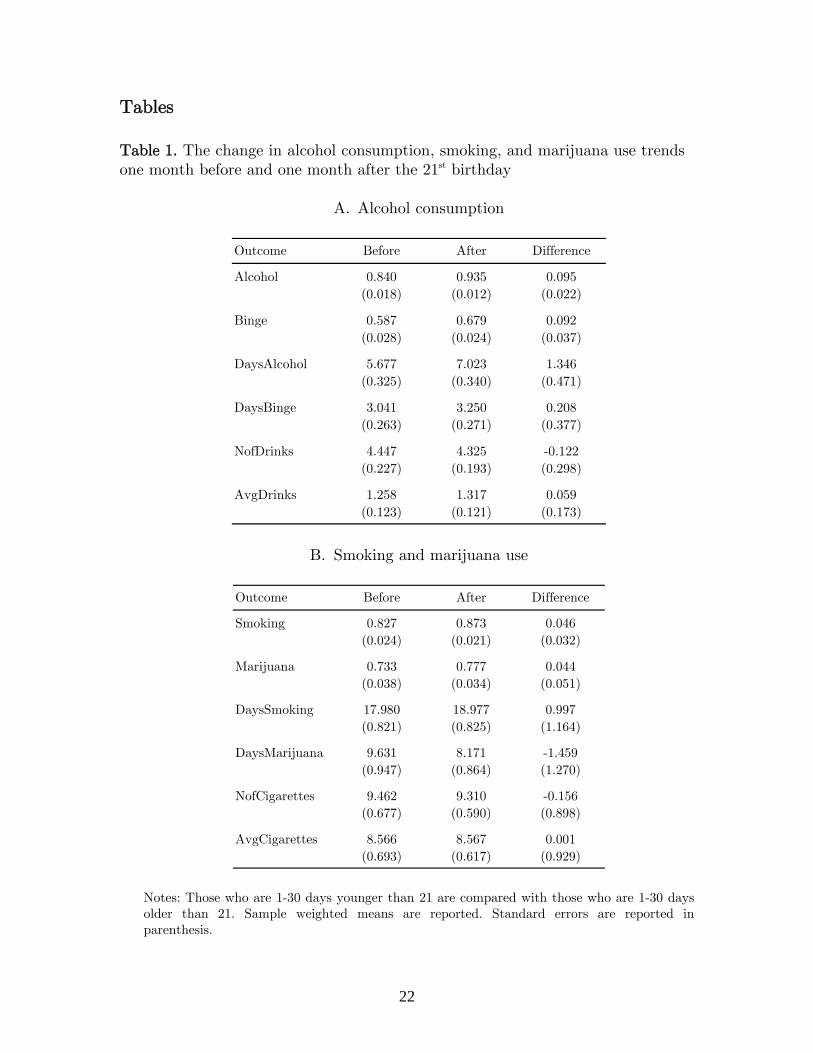
In the first panel of Table 1, we compare alcohol consumption patterns of young adults who are
about to turn 21 with those who had recently turned 21. In general, these raw numbers suggest
that young adults tend to increase their alcohol consumption once they turned 21. For instance,
the probability of drinking increases roughly 10 percentage points during the month following the
10Our choice of age bandwidth (19 to 22, inclusive) follows Carpenter and Dobkin (2009). The maximum sample size
is 29527. Since, our data contain information on some youths at more than one time period, in our empirical analysis,
we report the standard errors that are clustered at the individual level.11For instance, in National Health Interview Survey (NHIS), questions on alcohol consumption typically refer to the
prior 12 months with an option to report alcohol consumption over the past year, the past month, or the past week.12 We do not observe these binary variables directly. The respondents were asked the following questions: "During
the last 30 days, on how many days did you have one or more drinks of an alcoholic beverage?" and "On how many
days did you have five or more drinks on the same occasion during the past 30 days? By occasion we mean at the same
time or within hours of each other". The alcohol participation variables for the corresponding questions are coded unity
if the respondent reported consuming alcohol on at least one day during the past month and zero otherwise.13The respondents were asked the following question: "In the past 30 days, on the days you drank alcohol, about how
many drinks did you usually have?" In order to calculate the average number of drinks per day during a one month
period, we multiply the number of days that the respondent drank alcohol with the average number of drinks that she
had on those days and divide the result by 30.
7
21st birthday. Similarly, young adults are around 9 percentage points more likely to engage in binge
drinking, tend to consume alcohol 1.3 days more, and consume 0.1 drinks more on average once they
turn 21. However, as young adults are legally allowed to purchase alcohol, they tend to distribute
their alcohol consumption more evenly across days. Although, the number of days that they consume
alcohol increase, on average, they tend to have 0.1 drinks less on the days they consume alcohol.
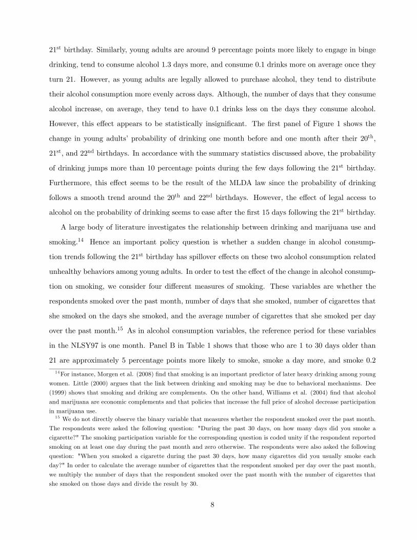
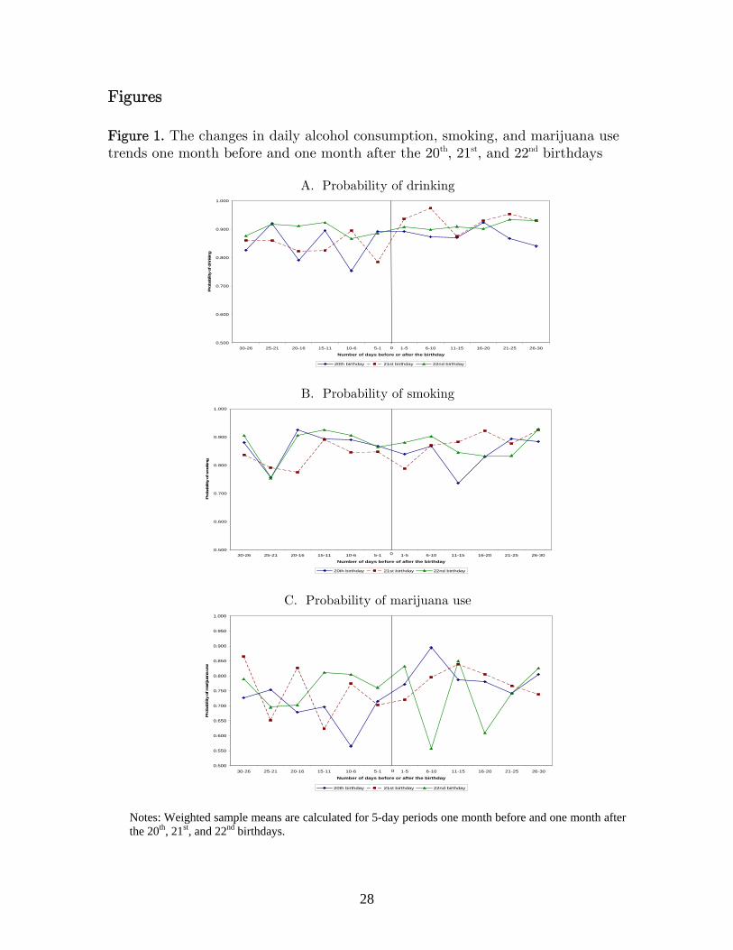
However, this effect appears to be statistically insignificant. The first panel of Figure 1 shows the
change in young adults’ probability of drinking one month before and one month after their 20th,
21st, and 22nd birthdays. In accordance with the summary statistics discussed above, the probability
of drinking jumps more than 10 percentage points during the few days following the 21st birthday.
Furthermore, this effect seems to be the result of the MLDA law since the probability of drinking
follows a smooth trend around the 20th and 22nd birthdays. However, the effect of legal access to
alcohol on the probability of drinking seems to ease after the first 15 days following the 21st birthday.
A large body of literature investigates the relationship between drinking and marijuana use and
smoking.14 Hence an important policy question is whether a sudden change in alcohol consump-
tion trends following the 21st birthday has spillover effects on these two alcohol consumption related
unhealthy behaviors among young adults. In order to test the effect of the change in alcohol consump-
tion on smoking, we consider four different measures of smoking. These variables are whether the
respondents smoked over the past month, number of days that she smoked, number of cigarettes that
she smoked on the days she smoked, and the average number of cigarettes that she smoked per day
over the past month.15 As in alcohol consumption variables, the reference period for these variables
in the NLSY97 is one month. Panel B in Table 1 shows that those who are 1 to 30 days older than
21 are approximately 5 percentage points more likely to smoke, smoke a day more, and smoke 0.2
14For instance, Morgen et al. (2008) find that smoking is an important predictor of later heavy drinking among young
women. Little (2000) argues that the link between drinking and smoking may be due to behavioral mechanisms. Dee
(1999) shows that smoking and driking are complements. On the other hand, Williams et al. (2004) find that alcohol
and marijuana are economic complements and that policies that increase the full price of alcohol decrease participation
in marijuana use.15 We do not directly observe the binary variable that measures whether the respondent smoked over the past month.
The respondents were asked the following question: "During the past 30 days, on how many days did you smoke a
cigarette?" The smoking participation variable for the corresponding question is coded unity if the respondent reported
smoking on at least one day during the past month and zero otherwise. The respondents were also asked the following
question: "When you smoked a cigarette during the past 30 days, how many cigarettes did you usually smoke each
day?" In order to calculate the average number of cigarettes that the respondent smoked per day over the past month,
we multiply the number of days that the respondent smoked over the past month with the number of cigarettes that
she smoked on those days and divide the result by 30.
8
less cigarettes on the days they smoke compared with those who are 1 to 30 days younger than 21.
However, these differences between the smoking habits of the two groups appear to be statistically
insignificant. The second panel of Figure 1 shows that the probability of smoking exhibits a declining
trend during the few days following the 21st birthday but increases later on. Overall, the probability
of smoking follows a relatively smooth trend around the 21st birthday. Compared with the 21st birth-
day, the probability of smoking trends around the 20th and 22nd birthdays are also similar suggesting
that an increase in alcohol consumption after the 21st birthday does not significantly affect smoking
habits of young adults.
To test the spillover effects of increased alcohol consumption following the 21st birthday on mar-
ijuana use, we use two different measures of marijuana use. These are whether the respondent used
marijuana over the past month and number of days that she used marijuana over the past month. The
second panel of Table 1 shows that young adults are 4 percentage points more likely to use marijuana
once they gain legal access to alcohol, but this effect is statistically insignificant. Similarly, although
the number of days that they use marijuana over the past month decreases by 1.5 days once they
turn 21, this effect is insignificant. Furthermore, panel C of Figure 1 shows that the probability of
marijuana use for those who are slightly older than 21 are slightly higher but in general comparable
with those of the respondents who are slightly older than 20 or 22.
4 Regression discontinuity design
We employ a RD design to estimate effect of the MLDA laws on alcohol consumption, marijuana use,
and smoking habits among young adults.16 This approach exploits the sudden increase in alcohol
consumption that occurs at age 21. Since alcohol purchase and consumption are legally allowed
according to this simple age cutoff, we are able to compare outcomes across youths with similar
income, educational attainment, and other observable individual characteristics, but very different
levels of alcohol use. The basic RD model used through our empirical analysis is as follows:
outcomei = β0Xi + δTi + f(agei) + εi (1)
16 Imbens and Lemieux (2008) and Lee and Lemieux (2009) present a detailed discussion of the RD design and related
issues.
9
where outcomei represents a particular youth outcome such as alcohol consumption, smoking, or
marijuana use by individual i. The vector of observable characteristics for individual i are denoted
by Xi and includes household income, educational attainment, marital status, gender, and race of the
respondent, binary controls for student and employment status, as well as a dummy variable which
controls for the birthday celebration effect and equals to one if the respondent was interviewed in the
month after turning 21.17 In general, these control variables vary smoothly over age 21. Hence, they
have little effect on our estimates of the discontinuity and serve mainly to increase the precision of our
estimates. The treatment variable is denoted by Ti and takes the value of unity if the respondent is at
least 21 years old at the interview date and zero otherwise. The coefficient δ, our main coefficient of
interest, indicates the effect of the MLDA law on the relevant outcome. Finally, f(agei) is a smooth
function of age profile, which is also known as the forcing variable in the context of RD design.18
Since, we observe the exact birth and interview date for each respondent, we were able to calculate
the difference between the interview date and the respondent’s 21st birthday in days. Therefore, for
each respondent, the variable agei represents the number of days before or after the 21st birthday.
Modelling the smooth function of age profile correctly is one of the main problems in implementing
the RD design. In order to address this problem, we consider both parametric and non-parametric
functions of age to explore the sensitivity of our results to a variety of functional form assumptions.
For our parametric specifications, we focus on linear, quadratic, cubic, and quartic models, allowing
the slope of these functions to vary on each side of the age cutoff (i.e. linear, quadratic, cubic,
and quartic splines). Hence, our general model with different degrees of polynomials that are fully
interacted with the treatment can be written as:
outcomei = β0Xi + δTi +kX
j=1
αjageji +
kXj=1
λj(Ti × ageji ) + εi for k = {1, 2, 3, 4}. (2)
For our non-parametric specifications, following Hahn, Todd, and van der Klaauw (2001) and
Porter(2003), we use local linear regressions to estimate the left and right limits of discontinuity at
age 21. The difference between the two limits is interpreted as the local treatment effect of the MLDA
law on outcome variables. Following Malamud and Pop-Eleches (2010), we estimate this in one step
17Appendix A provides the definition of control variables and their summary statistics. In addition to these control
variables, we also estimate models using year fixed effects as additional controls. Although not reported here, compared
with the reported results, these models produce similar estimated effect of the MLDA on outcome variables.18 In order to implement the RD design, we assume that the respondents do not have any control over the forcing
variable. Since our forcing variable is age, this condition is naturally satisfied.
10
using triangular kernel which has been shown to be boundary optimal by putting more weight on
observations closer to the cutoff point (Cheng, Fan, Marron, 1997).19
The remaining estimation issue for our non-parametric models is the selection of appropriate
bandwidth. Since the RD is identified only at the discontinuity, we try to balance the goals of staying
as local to the cutoff point at age 21 as possible while ensuring that we have enough data to yield
informative estimates. Since there is currently no widely agreed-upon method for selection of optimal
bandwidths in the nonparametric RD context, we follow Ludwig and Miller (2007) and present our
results for a broad range of candidate bandwidths. We start with a bandwidth of 240. However,
we also consider bandwidths that are twice (480), half (120), one fourth (60), and one eighth (30)
the size of this bandwidth.20 In our non-parametric models, we calculate the standard errors using
the bootstrap procedure with 1000 replications, which according to Cameron and Trivedi (2005) may
offer more accurate asymptotic inference than the analytic standard errors.
5 Results
This section reports the results of several parametric and non-parametric models estimated for dif-
ferent alcohol consumption, smoking, and marijuana use outcomes. We first test the possibility that
there exists other changes in observable characteristics of young adults occurring at age 21 that could
confound our analysis. In our context, this is equivalent to testing the smoothness of all control vari-
ables around the 21st birthday. Hence, we estimate equation (2) separately for all control variables
using a quadratic spline.21 The results reported in Table 2 suggests that for each covariate, the coef-
ficient of the treatment variable is insignificant and hence, there is no evidence of significant change
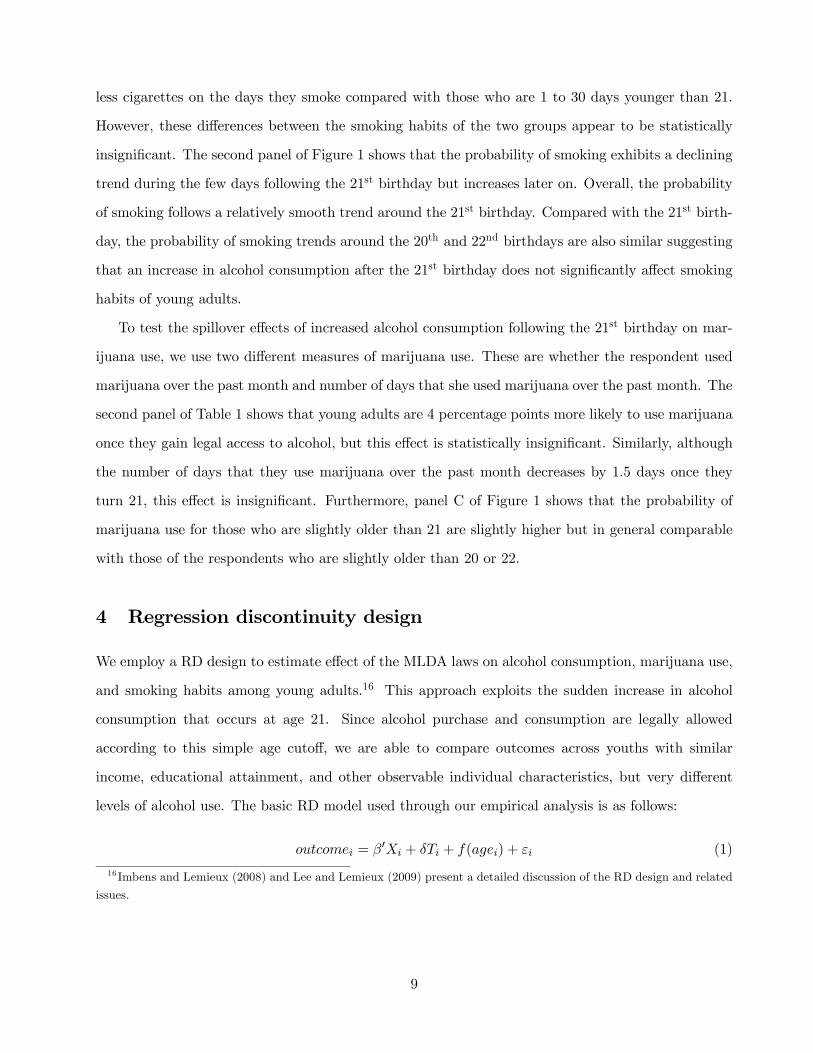
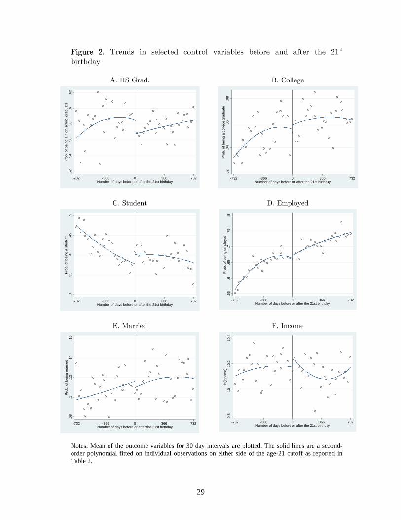
at the cutoff age of 21. We also graph the corresponding age profiles of selected control variables
19Lee and Lemuiex (2009) argue that an alternative way of putting more weight on observations close to the cutoff is
to re-estimate a non-parametric model with a rectangular kernel using smaller bandwidths. Following, Lee and Lemuiex
(2009), we also estimate our non-parametric models using rectangular kernel and smaller bandwidths. However, as in
previous studies, the choice of kernel has little effect on our estimates (Fan and Gijbels, 1996).20We also estimate our non-parametric models using the bandwidth selection procedure suggested by Imbens and
Kalyanarman (2009). The results were slightly higher but in general, comparable with the estimates presented in this
paper. However, we also observe that Imbens-Kalyanarman optimal bandwidths are extremely small and undersmooths
the data. Hence, the results are not reported here. The same problem is also discussed in Malamud and Pop-Eleches
(2010).21Following the previous literature, our selection of a quadratic polynomial is a result of a visual inspection of data
for the best fit. Estimating this model separately for all control variables using linear, cubic, or quartic splines yields
similar results. These results are available from the authors upon request.
11

in Figure 2. The quadratic prediction of each selected covariate appears to fit the actual data well
and exhibits either no or an insignificant small jump at age 21. Although, we cannot directly test
whether the unobservable characteristics of the young adults vary smoothly across the discontinuity,
our finding that observable characteristics are smoothly distributed around age 21 reduces the con-
cerns about omitted variables bias and suggests that parametric models estimated with or without
controls should yield similar results.22
Another possible concern to identification in a RD design comes from the possibility of nonrandom
sorting of young adults to either side of the age-21 cutoff. While this is highly unlikely, we examine
whether there is evidence of nonrandom sorting graphically. Appendix B shows the distribution of
observations around the age-21 cutoff. Overall, the distribution of the frequency of observations is
smooth across the minimum drinking age cutoff and hence, graphically there is little evidence of
nonrandom sorting around age 21.
5.1 Alcohol consumption
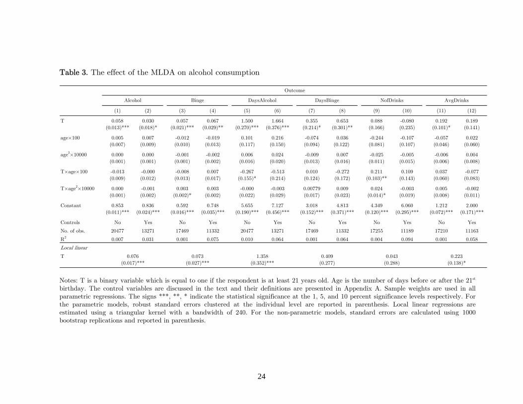
In the first two columns of Table 3, we report the estimates from parametric regressions of the effect
of the MLDA on the probability of alcohol consumption. These regressions are quadratic polynomials
in age fully interacted with a dummy variable indicating an age over 21 and estimated using sample
weights.23 Standard errors are clustered at the individual level to correct for the non-independence of
individual observations over time. The first specification estimated without control variables suggests
that the age-21 discontinuity is associated with an approximate 6 percentage point increase in the
probability of drinking. Furthermore, this effect is highly significant. The second specification adds
a set of control variables to the regression as discussed in equation (2). Inclusion of these control
variables decreases the effect of the MLDA on the probability of drinking by around 3 percentage
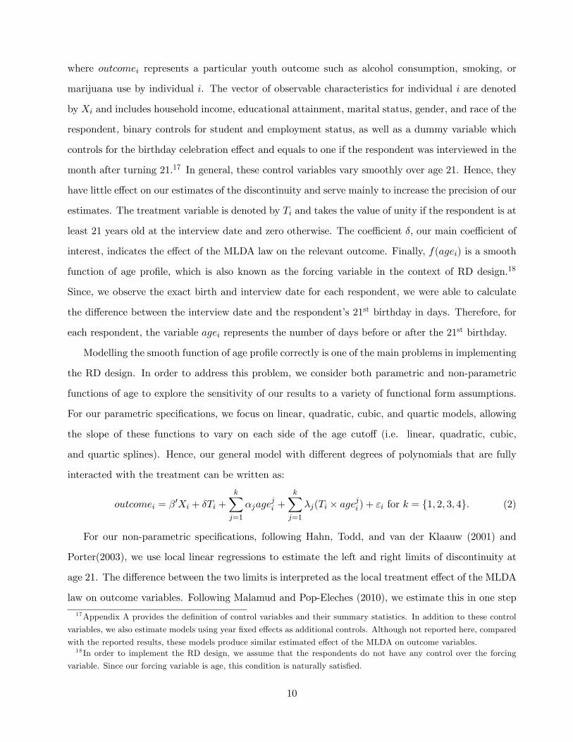
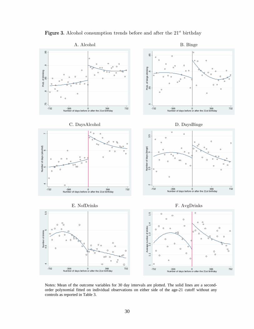
points. In panel A of Figure 3, we superimpose the quadratic fitted lines from the parametric model
estimated without any controls over the mean value of the percent of drinkers calculated for each 30-
22Since the empirical results are based on self-reported survey data, youths under the MLDA may also be more likely
to underreport their alcohol consumption since alcohol consumption is illegal for those who are under 21. This could
generate a discrete jump in reported level of alcohol consumption at age 21 even if there is no true change in actual
behavior. However, as documented in Figure 1, the reported alcohol consumption patterns of 20-year-olds are very
similar compared with 21 and 22-year-olds, which suggests that the empirical results documented in this paper are not
subject to a underreporting bias.23Although not reported here, comparable parametric models estimated without sample weights yield similar results.
12
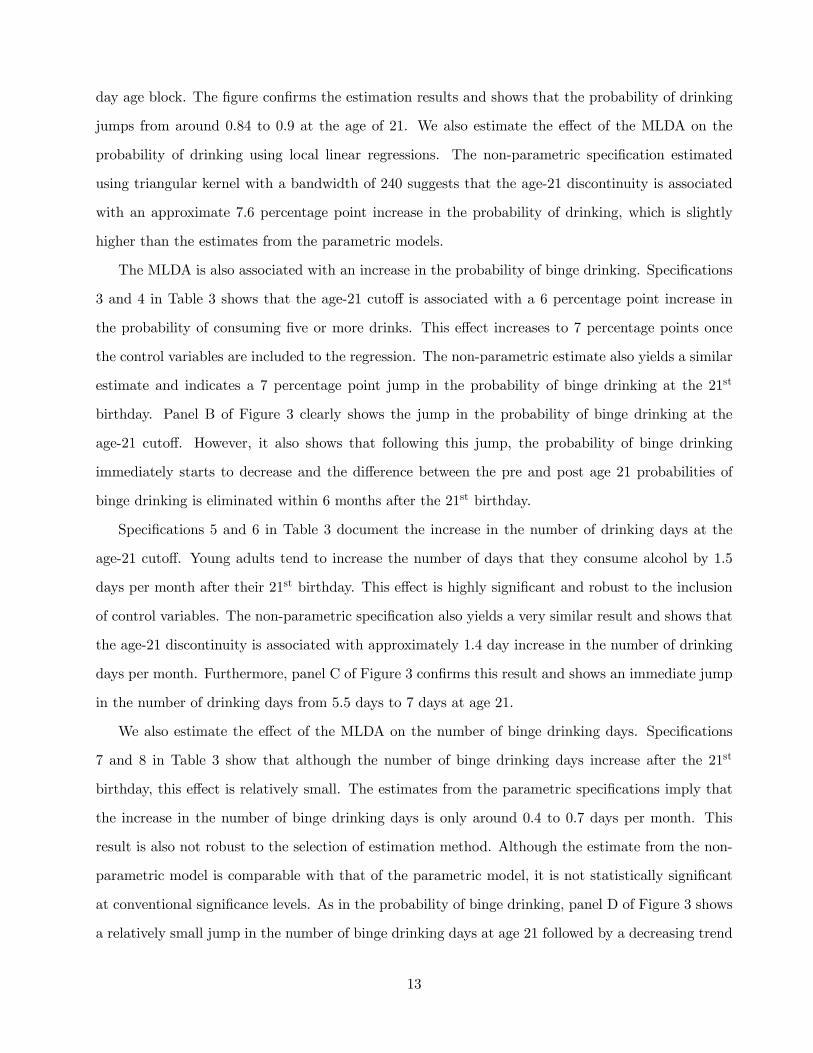
day age block. The figure confirms the estimation results and shows that the probability of drinking
jumps from around 0.84 to 0.9 at the age of 21. We also estimate the effect of the MLDA on the
probability of drinking using local linear regressions. The non-parametric specification estimated
using triangular kernel with a bandwidth of 240 suggests that the age-21 discontinuity is associated
with an approximate 7.6 percentage point increase in the probability of drinking, which is slightly
higher than the estimates from the parametric models.
The MLDA is also associated with an increase in the probability of binge drinking. Specifications
3 and 4 in Table 3 shows that the age-21 cutoff is associated with a 6 percentage point increase in
the probability of consuming five or more drinks. This effect increases to 7 percentage points once
the control variables are included to the regression. The non-parametric estimate also yields a similar
estimate and indicates a 7 percentage point jump in the probability of binge drinking at the 21st
birthday. Panel B of Figure 3 clearly shows the jump in the probability of binge drinking at the
age-21 cutoff. However, it also shows that following this jump, the probability of binge drinking
immediately starts to decrease and the difference between the pre and post age 21 probabilities of
binge drinking is eliminated within 6 months after the 21st birthday.
Specifications 5 and 6 in Table 3 document the increase in the number of drinking days at the
age-21 cutoff. Young adults tend to increase the number of days that they consume alcohol by 1.5
days per month after their 21st birthday. This effect is highly significant and robust to the inclusion
of control variables. The non-parametric specification also yields a very similar result and shows that
the age-21 discontinuity is associated with approximately 1.4 day increase in the number of drinking
days per month. Furthermore, panel C of Figure 3 confirms this result and shows an immediate jump
in the number of drinking days from 5.5 days to 7 days at age 21.
We also estimate the effect of the MLDA on the number of binge drinking days. Specifications
7 and 8 in Table 3 show that although the number of binge drinking days increase after the 21st
birthday, this effect is relatively small. The estimates from the parametric specifications imply that
the increase in the number of binge drinking days is only around 0.4 to 0.7 days per month. This
result is also not robust to the selection of estimation method. Although the estimate from the non-
parametric model is comparable with that of the parametric model, it is not statistically significant
at conventional significance levels. As in the probability of binge drinking, panel D of Figure 3 shows
a relatively small jump in the number of binge drinking days at age 21 followed by a decreasing trend
13
in binge drinking. Similarly, the difference between the pre and post age 21 binge drinking habits is
eliminated within 6 months after the 21st birthday.
In contrast to the other measures of alcohol consumption, the effect of the MLDA on the number
of drinks that young adults had on the days they consumed alcohol is insignificant. Specification 10
in Table 3 shows that once they turn 21, young adults tend to distribute their alcohol consumption
more evenly by consuming alcohol on more days, but drinking around 0.1 less drinks on the days they
consume alcohol. However, This effect is not statistically significant. The last two columns in Table 3
shows that at age 21, the average number of drinks per day still increases by 0.2. Although, this effect
is robust to the selection of non-parametric specification, it is not robust to the inclusion of control
variables. Panel F of Figure 3 shows a small increase in the average number of drinks consumed per
day due to the MLDA. This increase vanishes over time, however.
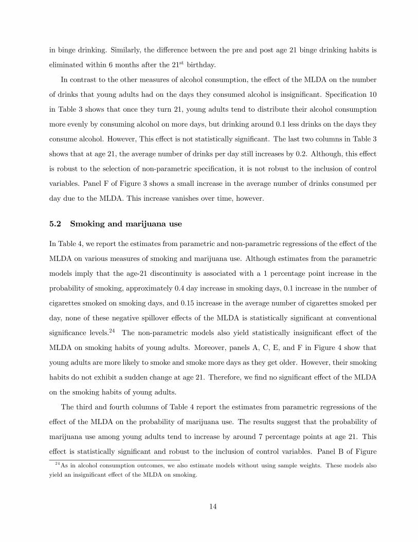
5.2 Smoking and marijuana use
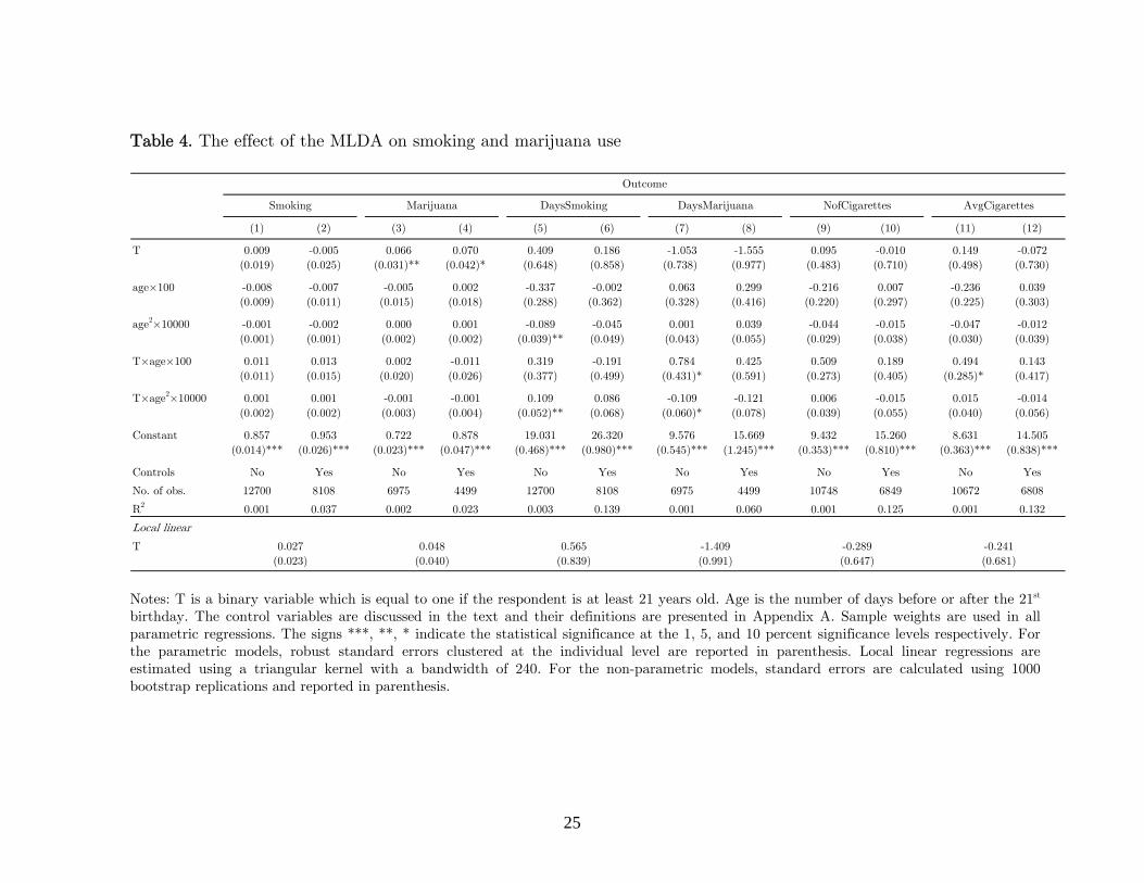
In Table 4, we report the estimates from parametric and non-parametric regressions of the effect of the
MLDA on various measures of smoking and marijuana use. Although estimates from the parametric
models imply that the age-21 discontinuity is associated with a 1 percentage point increase in the
probability of smoking, approximately 0.4 day increase in smoking days, 0.1 increase in the number of
cigarettes smoked on smoking days, and 0.15 increase in the average number of cigarettes smoked per
day, none of these negative spillover effects of the MLDA is statistically significant at conventional
significance levels.24 The non-parametric models also yield statistically insignificant effect of the
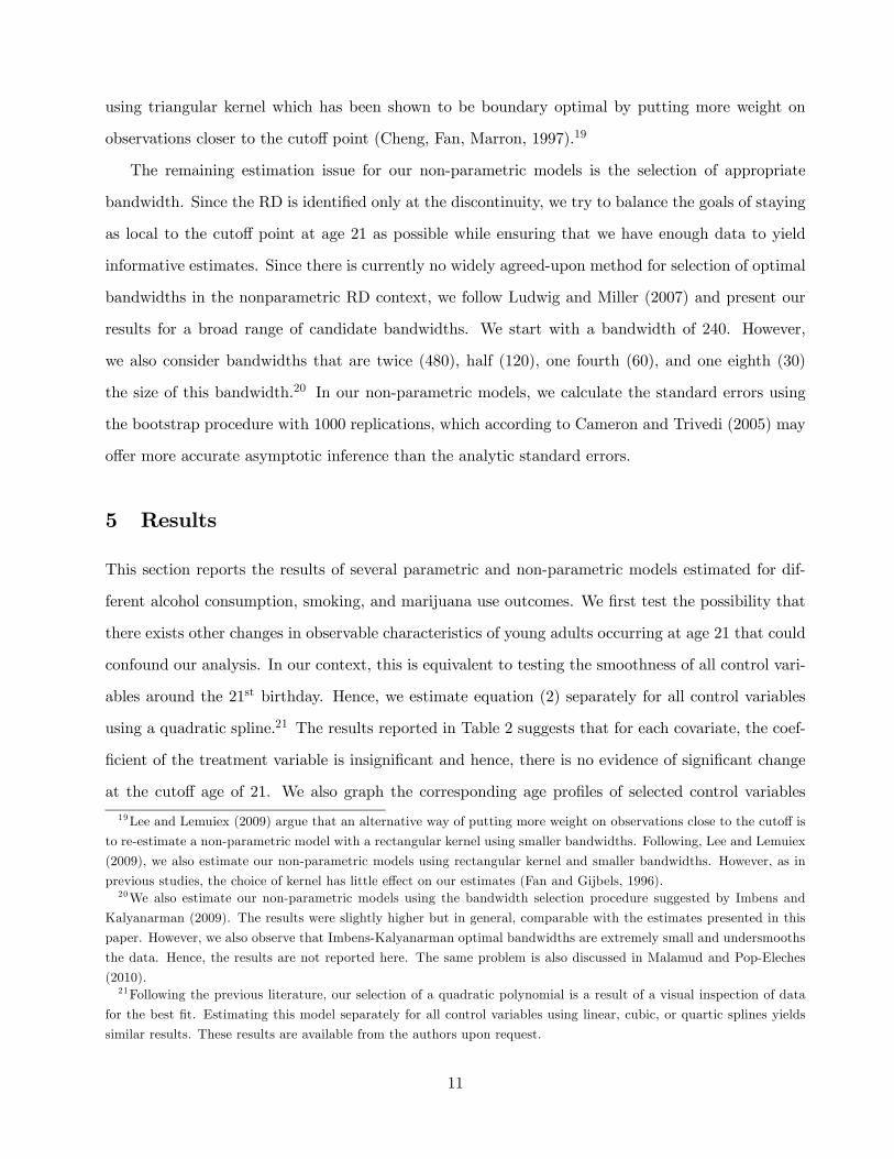
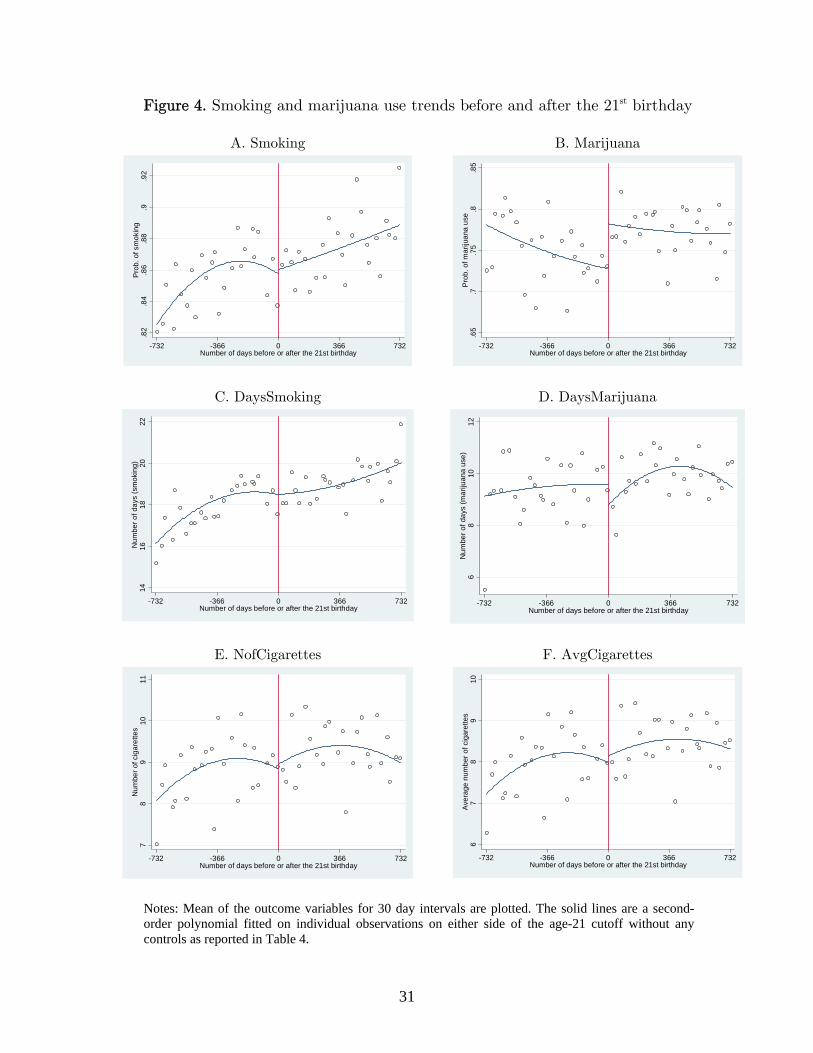
MLDA on smoking habits of young adults. Moreover, panels A, C, E, and F in Figure 4 show that
young adults are more likely to smoke and smoke more days as they get older. However, their smoking
habits do not exhibit a sudden change at age 21. Therefore, we find no significant effect of the MLDA
on the smoking habits of young adults.
The third and fourth columns of Table 4 report the estimates from parametric regressions of the
effect of the MLDA on the probability of marijuana use. The results suggest that the probability of
marijuana use among young adults tend to increase by around 7 percentage points at age 21. This
effect is statistically significant and robust to the inclusion of control variables. Panel B of Figure
24As in alcohol consumption outcomes, we also estimate models without using sample weights. These models also
yield an insignificant effect of the MLDA on smoking.
14

4 also shows a jump in the probability of marijuana use at the age-21 cutoff. Furthermore, the
increase in the probability of marijuana use among young adults after their 21st birthday appears
to be persistent in the long run. The estimate from the local linear regression also implies that the
age-21 discontinuity is associated with an approximate 5 percentage point increase in the probability
of marijuana use. This effect is not significant at conventional significance levels, however.
In panels 7 and 8 of Table 4, we investigate the effect of the MLDA on the number of days that
the respondents used marijuana in the last month. Although the estimates from the parametric and
non-parametric models suggest that the MLDA is associated with slightly more than a 1 day decrease
in the number of days of marijuana use, this effect is not statistically significant. Panel D of Figure
4 confirms this result and shows that pre and post age 21 trends in the number of days of marijuana
use exhibit similar trends.
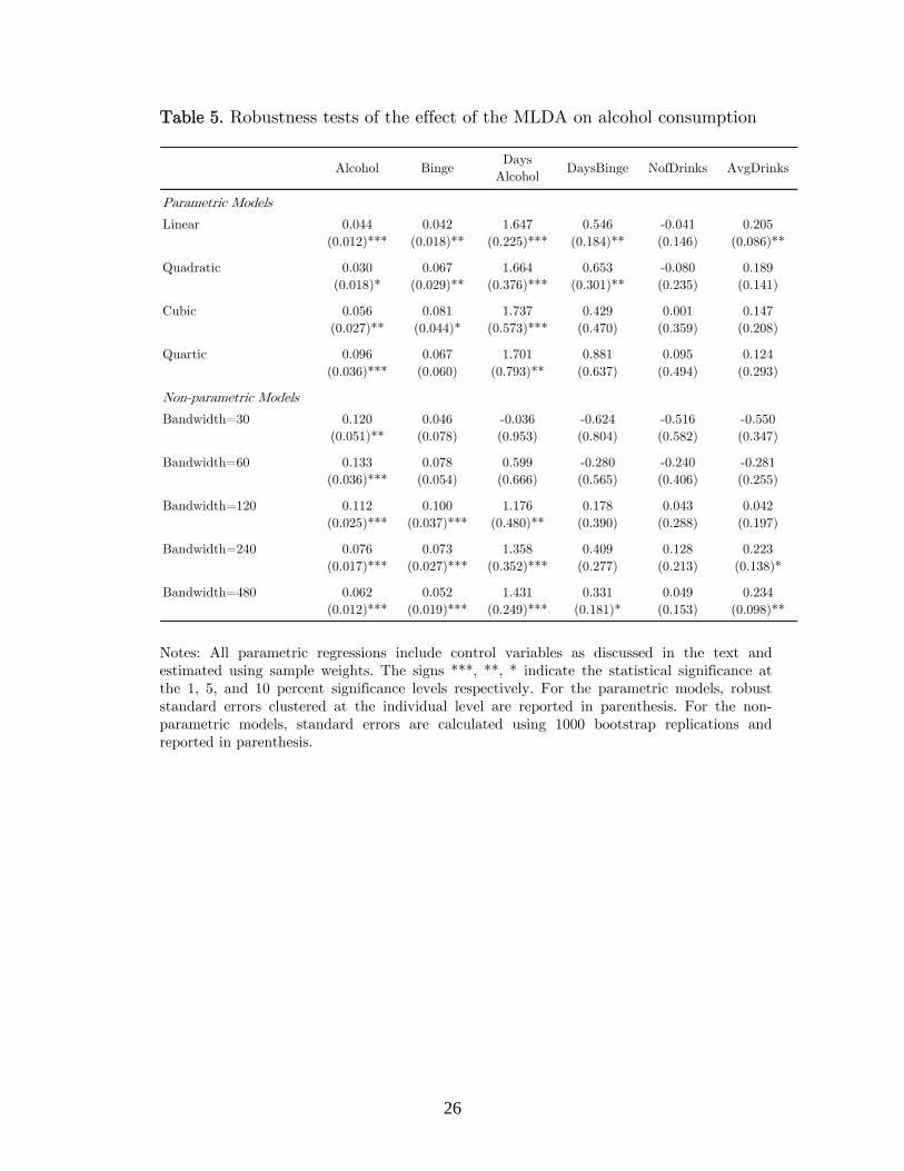
5.3 Robustness checks
In this section, we investigate whether the results from our preferred parametric and non-parametric
models are sensitive to the model specification. In particular, for parametric models, we test the
robustness of our results to the selection of the degree of polynomial and for non-parametric models, we
test the sensitivity of our results to the bandwidth selection. Overall, our results from the parametric
models are robust to the selection of the degree of polynomial. The results from the non-parametric
models are mixed, but are mostly comparable with the estimates of the parametric models. In
particular, the results from the non-parametric models estimated using relatively larger bandwidths
are very similar to those from the parametric models.
The first column in Table 5 shows that the effect of the MLDA on probability of drinking is robust
to the selection of the degree of polynomial in parametric models. The estimates from alternative
models suggest that the probability of drinking among young adults tend to increase 3 to 10 percent-
age points at age 21. In general, estimates from the non-parametric models yield a larger effect of
the MLDA on the probability of drinking. These models estimated using several different bandwidths
ranging from 30 to 480 show that young adults tend to increase their probability of alcohol consump-
tion by around 6 to 13 percentage points after their 21st birthday. The second column in Table 5
shows that under several different parametric specifications, the age-21 cutoff is also associated with
a 4 to 8 percentage point increase in the probability of binge drinking. In general, the non-parametric
15
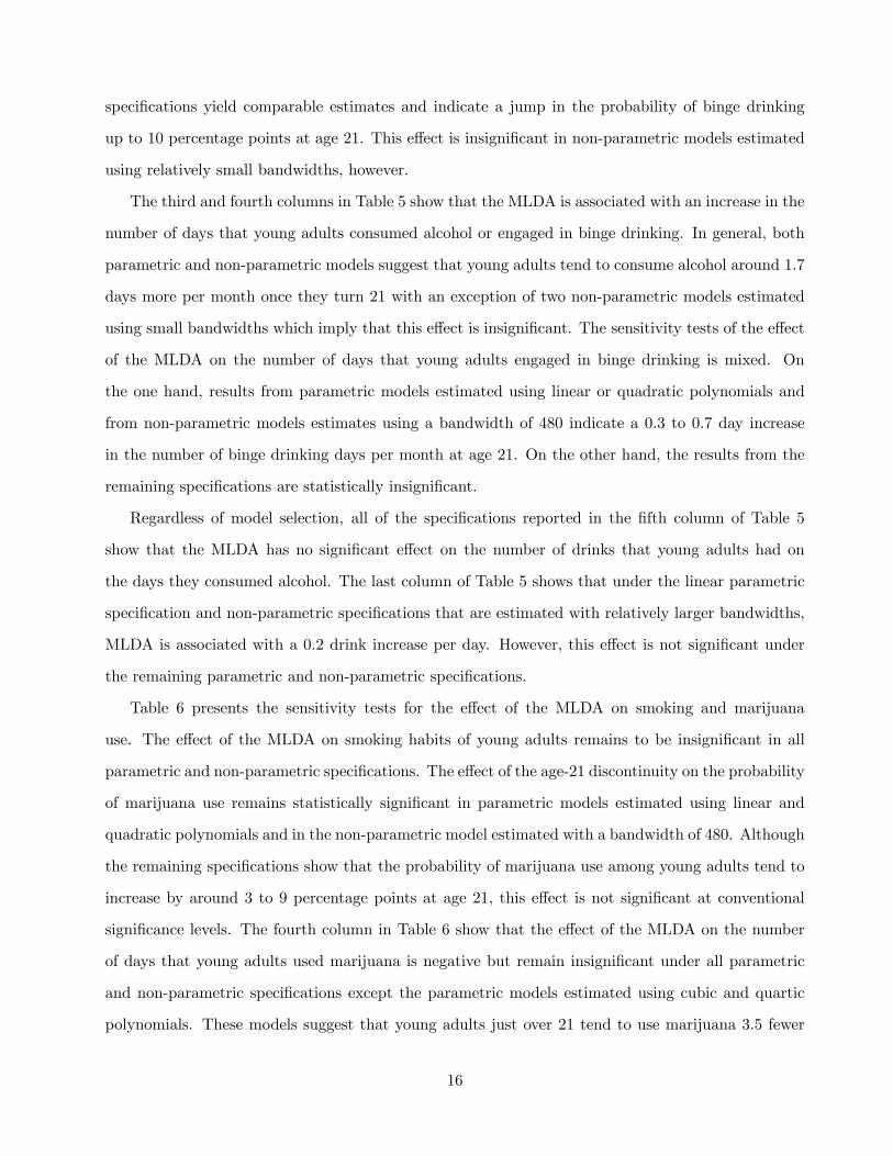
specifications yield comparable estimates and indicate a jump in the probability of binge drinking
up to 10 percentage points at age 21. This effect is insignificant in non-parametric models estimated
using relatively small bandwidths, however.
The third and fourth columns in Table 5 show that the MLDA is associated with an increase in the
number of days that young adults consumed alcohol or engaged in binge drinking. In general, both
parametric and non-parametric models suggest that young adults tend to consume alcohol around 1.7
days more per month once they turn 21 with an exception of two non-parametric models estimated
using small bandwidths which imply that this effect is insignificant. The sensitivity tests of the effect
of the MLDA on the number of days that young adults engaged in binge drinking is mixed. On
the one hand, results from parametric models estimated using linear or quadratic polynomials and
from non-parametric models estimates using a bandwidth of 480 indicate a 0.3 to 0.7 day increase
in the number of binge drinking days per month at age 21. On the other hand, the results from the
remaining specifications are statistically insignificant.
Regardless of model selection, all of the specifications reported in the fifth column of Table 5
show that the MLDA has no significant effect on the number of drinks that young adults had on
the days they consumed alcohol. The last column of Table 5 shows that under the linear parametric
specification and non-parametric specifications that are estimated with relatively larger bandwidths,
MLDA is associated with a 0.2 drink increase per day. However, this effect is not significant under
the remaining parametric and non-parametric specifications.
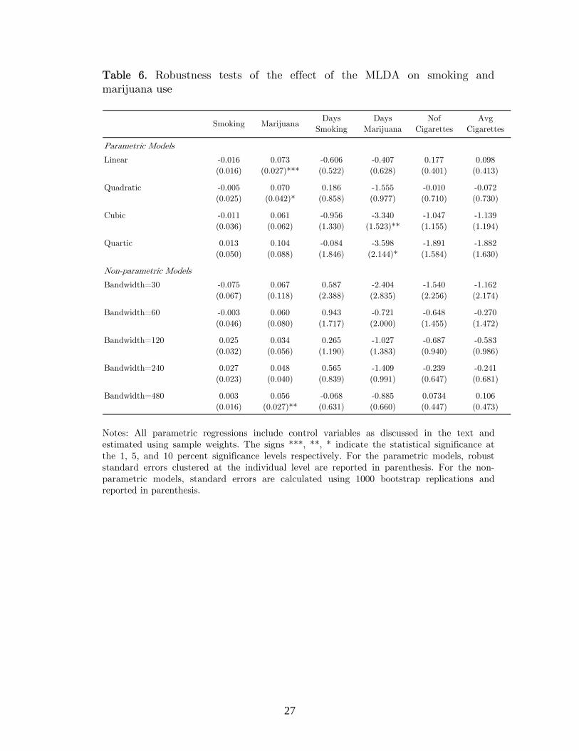
Table 6 presents the sensitivity tests for the effect of the MLDA on smoking and marijuana
use. The effect of the MLDA on smoking habits of young adults remains to be insignificant in all
parametric and non-parametric specifications. The effect of the age-21 discontinuity on the probability
of marijuana use remains statistically significant in parametric models estimated using linear and
quadratic polynomials and in the non-parametric model estimated with a bandwidth of 480. Although
the remaining specifications show that the probability of marijuana use among young adults tend to
increase by around 3 to 9 percentage points at age 21, this effect is not significant at conventional
significance levels. The fourth column in Table 6 show that the effect of the MLDA on the number
of days that young adults used marijuana is negative but remain insignificant under all parametric
and non-parametric specifications except the parametric models estimated using cubic and quartic
polynomials. These models suggest that young adults just over 21 tend to use marijuana 3.5 fewer
16
days compared with those who are just under 21.25
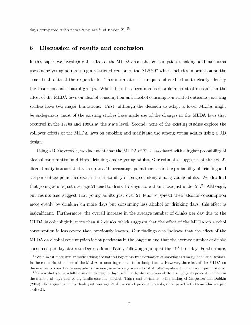
6 Discussion of results and conclusion
In this paper, we investigate the effect of the MLDA on alcohol consumption, smoking, and marijuana
use among young adults using a restricted version of the NLSY97 which includes information on the
exact birth date of the respondents. This information is unique and enabled us to clearly identify
the treatment and control groups. While there has been a considerable amount of research on the
effect of the MLDA laws on alcohol consumption and alcohol consumption related outcomes, existing
studies have two major limitations. First, although the decision to adopt a lower MLDA might
be endogenous, most of the existing studies have made use of the changes in the MLDA laws that
occurred in the 1970s and 1980s at the state level. Second, none of the existing studies explore the
spillover effects of the MLDA laws on smoking and marijuana use among young adults using a RD
design.
Using a RD approach, we document that the MLDA of 21 is associated with a higher probability of
alcohol consumption and binge drinking among young adults. Our estimates suggest that the age-21
discontinuity is associated with up to a 10 percentage point increase in the probability of drinking and
a 8 percentage point increase in the probability of binge drinking among young adults. We also find
that young adults just over age 21 tend to drink 1.7 days more than those just under 21.26 Although,
our results also suggest that young adults just over 21 tend to spread their alcohol consumption
more evenly by drinking on more days but consuming less alcohol on drinking days, this effect is
insignificant. Furthermore, the overall increase in the average number of drinks per day due to the
MLDA is only slightly more than 0.2 drinks which suggests that the effect of the MLDA on alcohol
consumption is less severe than previously known. Our findings also indicate that the effect of the
MLDA on alcohol consumption is not persistent in the long run and that the average number of drinks
consumed per day starts to decrease immediately following a jump at the 21st birthday. Furthermore,
25We also estimate similar models using the natural logarithm transformation of smoking and marijuana use outcomes.
In these models, the effect of the MLDA on smoking remain to be insignificant. However, the effect of the MLDA on
the number of days that young adults use marijuana is negative and statistically significant under most specifications.26Given that young adults drink on average 6 days per month, this corresponds to a roughly 25 percent increase in
the number of days that young adults consume alcohol. This result is similar to the finding of Carpenter and Dobkin
(2009) who argue that individuals just over age 21 drink on 21 percent more days compared with those who are just
under 21.
17
these results are robust to selection of several alternative parametric and non-parametric models.
We also provide new estimates of the relationship between alcohol consumption and smoking and
marijuana use which complements the existing literature. Similar to alcohol consumption, the spillover
effects of the MLDA on smoking and marijuana use among young adults is limited as well. We find
that the smoking trends of young adults vary smoothly across the age-21 cutoff which suggests that
the MLDA has no significant effect on smoking. However, the probability of marijuana use among
young adults tend to increase by around 7 percentage points under certain specifications. These
findings are particularly important given the ongoing public policy debates about stricter alcohol
control targeted at youths. Our results indicate policies that combat drinking may have desirable
impacts and can create public health benefits and that stricter alcohol control targeted toward young
adults could result in meaningful reductions in alcohol consumption. However, given that average
alcohol consumption, smoking, and marijuana use of young adults mostly appear to be unaffected by
the MLDA laws, such policies may have limited impact in reducing substance abuse among young
adults.
In this paper, although we document the relationship between the MLDA and smoking and mari-
juana use, we could not explore the spillover effects of the MLDA laws on other alcohol consumption
related outcomes such as drug abuse, alcohol related traffic accidents, and criminal behavior mostly
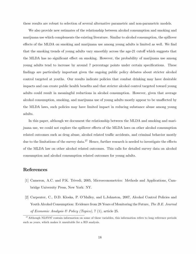
due to the limitations of the survey data.27 Hence, further research is needed to investigate the effects
of the MLDA law on other alcohol related outcomes. This calls for detailed survey data on alcohol
consumption and alcohol consumption related outcomes for young adults.
References
[1] Cameron, A.C. and P.K. Trivedi, 2005, Microeconometrics: Methods and Applications, Cam-
bridge University Press, New York: NY.
[2] Carpenter, C., D.D. Kloska, P. O’Malley, and L.Johnston, 2007, Alcohol Control Policies and
Youth Alcohol Consumption: Evidence from 28 Years of Monitoring the Future, The B.E. Journal
of Economic Analysis & Policy (Topics), 7 (1), article 25.
27Although NLSY97 contain information on some of these variables, this information refers to long reference periods
such as years, which makes it unsuitable for a RD analysis.
18
[3] Carpenter, C. and C. Dobkin, 2008, The drinking age, alcohol consumption, and crime, Unpub-
lished Manuscript, University of California at Irvine, The Paul Merage School of Business.
[4] Carpenter, C. and C. Dobkin, 2009, The effect of alcohol consumption on mortality: Regression
discontinuity evidence from the minimum drinking age, American Economic Journal: Applied
Economics, 1, 164-182.
[5] Chaloupka, F.J. and A. Laixuthai, 1997, Do youths substitute alcohol and marijuana? Some
econometric evidence, Eastern Economic Journal, 23, 253-276.
[6] Cheng, M.Y., J. Fan, and J.S. Marron, 1997, On automatic boundary correction, Annals of
Statistics, 25, 1691-1708.
[7] Dee, T.S., 1999, The complementarity of teen smoking and drinking, Journal of Health Eco-
nomics, 18, 769-793.
[8] Dee, T.S. and W.N. Evans, 2003, Teen drinking and educational attainment: Evidence from
two-sample instrumental variables estimates, Journal of Labor Economics, 21, 178-209.
[9] DiNardo, J.E. and T. Lemieux, 2001, Alcohol, marijuana, and American youth: The unintended
consequences of government regulation, Journal of Health Economics, 20, 991-1010.
[10] Fan, J, and I. Gijbels, Local Polynomial Modelling and Its Applications, Chapman and Hall,
London: UK.
[11] Goel, R.K. and M.J. Morey, 1995, The interdependence of cigarette and liquor demand, Southern
Economic Journal, 62, 441-459.
[12] Hahn, J., P. Todd, and W. van der Klaauw, 2001, Identification and estimation of treatment
effects with a regression-discontinuity design, Econometrica, 69, 201-209.
[13] Hansagi, H. et al., 1995, Alcohol consumption and stroke mortality, Stroke, 26, 1768-1773.
[14] Imbens, G. and K. Kalyanamaran, 2009, Optimal bandwidth choice for the regression disconti-
nuity estimator, NBER Working Paper No. 14723.
[15] Imbens, G. and T. Lemieux, 2008, Regression discontinuity designs: A guide to practice, Journal
of Econometrics, 142, 615-635.
19
[16] Kreft, S.F. and N.M. Epling, 2007, Do border crossings contribute to underage motor-vehicle
fatalities? An analysis of Michigan border crossings, Canadian Journal of Economics, 40, 765-
781.
[17] Laixuthai, A. and F.J. Chaloupka, 1993, Youth alcohol use and public policy, Contemporary
Economic Policy, 11, 70-81.
[18] Lee, D.S. and T. Lemieux, 2009, Regression discontinuity designs in economics, NBER Working
Paper No. 02138.
[19] Little, H.J., 2000, Behavioral mechanisms underlying the link between smoking and drinking,
Alcohol Research and Health, 24, 215-224.
[20] Lovenheim, M.F. and J. Slemrod, 2010, The fatal toll of driving to drink: The effect of minimum
legal drinking age evasion on traffic fatalities, Journal of Health Economics, 29, 62-77.
[21] Ludwig, J. and D. Miller, 2007, Does head start improve children’s life chances? Evidence from
a regression discontinuity design, Quarterly Journal of Economics, 122, 159-208.
[22] Malamud, O. and C. Pop-Eleches, 2010, Home computer use and the development of human
capital, forthcoming in Quarterly Journal of Economics.
[23] Mann, R.E., R.G. Smart, and R. Govoni, 2003, The epidemiology of alcoholic liver disease.
Alcohol Research & Health, 27, 209—219.
[24] Markowitz, S., 2005, Alcohol, drugs, and violent crime, International Review of Law and Eco-
nomics, 25, 20-44.
[25] Miron, J.A. and E. Tetelbaum, 2009, Does the minimum legal drinking age save lives?, Economic
Inquiry, 47, 317-336.
[26] Morgen, C.S. et al., 2008, Association between smoking and the risk of heavy drinking among
young women: A prospective study, Alcohol and Alcoholism, 43, 371-375.
[27] Nicholson, W.M. and H.M. Taylor, 1940, Blood volume studies in acute alcoholism, Quarterly
Journal of Studies on Alcohol, 1, 472.
20

[28] Pacula, L.R., 1998, Does increasing the beer tax reduce marijuana consumption?, Journal of
Health Economics, 17, 557-585.
[29] Poikolainen, K., 1996, Alcohol and overall health outcomes, Annals of Medicine, 28, 381-384.
[30] Porter, J., 2003, Estimation in the regression discontinuity model, Unpublished Manuscript,
Harvard University, Department of Economics.
[31] Williams, J., R. Liccardo Pacula, F.J. Chaloupka, and H.Wechsler, 2004, Alcohol and marijuana
use among college students: economic complement or substitutes, Health Economics, 13, 825-843.
[32] Wagenaar, A.C. and T.L. Toomey, 2002, Effects of minimum drinking age laws: Review and
analyses of the literature from 1960 to 2000, Journal of Studies on Alcohol, 14, 206-225.
21
22
Tables Table 1. The change in alcohol consumption, smoking, and marijuana use trends one month before and one month after the 21st birthday
A. Alcohol consumption
Outcome Before After Difference
Alcohol 0.840 0.935 0.095(0.018) (0.012) (0.022)
Binge 0.587 0.679 0.092(0.028) (0.024) (0.037)
DaysAlcohol 5.677 7.023 1.346(0.325) (0.340) (0.471)
DaysBinge 3.041 3.250 0.208(0.263) (0.271) (0.377)
NofDrinks 4.447 4.325 -0.122(0.227) (0.193) (0.298)
AvgDrinks 1.258 1.317 0.059(0.123) (0.121) (0.173)
B. Smoking and marijuana use
Outcome Before After Difference
Smoking 0.827 0.873 0.046(0.024) (0.021) (0.032)
Marijuana 0.733 0.777 0.044(0.038) (0.034) (0.051)
DaysSmoking 17.980 18.977 0.997(0.821) (0.825) (1.164)
DaysMarijuana 9.631 8.171 -1.459(0.947) (0.864) (1.270)
NofCigarettes 9.462 9.310 -0.156(0.677) (0.590) (0.898)
AvgCigarettes 8.566 8.567 0.001(0.693) (0.617) (0.929)
Notes: Those who are 1-30 days younger than 21 are compared with those who are 1-30 days older than 21. Sample weighted means are reported. Standard errors are reported in parenthesis.

23
Table 2. Test of the smoothness of the control variables around the 21st birthday
HS Grad. GEDSome
CollegeCollege Graduate Student ln(Income) Black Hispanic Female Employed Married
T -0.028 -0.011 -0.003 0.002 -0.002 0.015 0.055 -0.009 -0.001 0.014 0.019 0.000(0.017) (0.008) (0.006) (0.009) (0.002) (0.018) (0.076) (0.008) (0.008) (0.015) (0.016) (0.012)
age×100 -0.003 0.010 0.002 -0.002 0.001 0.000 0.002 0.000 0.006 -0.003 -0.011 0.001(0.008) (0.004)*** (0.003) (0.004) (0.001) (0.008) (0.037) (0.003) (0.003)* (0.006) (0.007) (0.005)
age2×10000 -0.001 0.001 0.000 -0.001 0.000 0.001 -0.002 0.000 0.001 0.000 -0.003 0.000(0.001) (0.000)* (0.000) (0.001) (0.000) (0.001) (0.005) (0.000) (0.000)** (0.001) (0.001)*** (0.001)
T×age×100 0.007 -0.010 -0.003 0.006 -0.001 0.009 -0.093 0.007 -0.009 -0.001 0.022 0.002(0.011) (0.005)** (0.004) (0.006) (0.001) (0.010) (0.050)* (0.004) (0.004)** (0.007) (0.009)*** (0.007)
T×age2×10000 0.001 -0.001 0.000 0.000 0.000 -0.002 0.013 -0.001 0.000 0.001 0.003 0.000(0.001) (0.001)* (0.000) (0.001) (0.000) (0.001) (0.007)* (0.001) (0.001) (0.001) (0.001)** (0.001)
Constant 0.602 0.078 0.034 0.067 0.004 0.400 10.349 0.153 0.133 0.485 0.678 0.121(0.012)*** (0.006)*** (0.004)*** (0.007)*** (0.001)*** (0.013)*** (0.054) (0.006)*** (0.006)*** (0.011)*** (0.011)*** (0.008)***
No. of obs. 27698 27698 27698 27698 27698 27679 19939 29527 29527 29527 29526 26877R2 0.0003 0.0003 0.0006 0.0016 0.0004 0.0026 0.0005 0.0001 0.0001 0.0001 0.0081 0.0009
Outcome
Notes: T is a binary variable which is equal to one if the respondent is at least 21 years old. Age is the number of days before or after the 21st birthday. Sample weights are used in all regressions. The signs ***, **, * indicate the statistical significance at the 1, 5, and 10 percent significance level respectively. Robust standard errors clustered at the individual level are reported in parenthesis.
24
Table 3. The effect of the MLDA on alcohol consumption
(1) (2) (3) (4) (5) (6) (7) (8) (9) (10) (11) (12)
T 0.058 0.030 0.057 0.067 1.500 1.664 0.355 0.653 0.088 -0.080 0.192 0.189(0.013)*** (0.018)* (0.021)*** (0.029)** (0.270)*** (0.376)*** (0.214)* (0.301)** (0.166) (0.235) (0.101)* (0.141)
age×100 0.005 0.007 -0.012 -0.019 0.101 0.216 -0.074 0.036 -0.244 -0.107 -0.057 0.022(0.007) (0.009) (0.010) (0.013) (0.117) (0.150) (0.094) (0.122) (0.081) (0.107) (0.046) (0.060)
age2×10000 0.000 0.000 -0.001 -0.002 0.006 0.024 -0.009 0.007 -0.025 -0.005 -0.006 0.004(0.001) (0.001) (0.001) (0.002) (0.016) (0.020) (0.013) (0.016) (0.011) (0.015) (0.006) (0.008)
T×age×100 -0.013 -0.000 -0.008 0.007 -0.267 -0.513 0.010 -0.272 0.211 0.109 0.037 -0.077(0.009) (0.012) (0.013) (0.017) (0.155)* (0.214) (0.124) (0.172) (0.103)** (0.143) (0.060) (0.083)
T×age2×10000 0.000 -0.001 0.003 0.003 -0.000 -0.003 0.00779 0.009 0.024 -0.003 0.005 -0.002(0.001) (0.002) (0.002)* (0.002) (0.022) (0.029) (0.017) (0.023) (0.014)* (0.019) (0.008) (0.011)
Constant 0.853 0.836 0.592 0.748 5.655 7.127 3.018 4.813 4.349 6.060 1.212 2.000(0.011)*** (0.024)*** (0.016)*** (0.035)*** (0.190)*** (0.456)*** (0.152)*** (0.371)*** (0.120)*** (0.295)*** (0.072)*** (0.171)***
Controls No Yes No Yes No Yes No Yes No Yes No Yes
No. of obs. 20477 13271 17469 11332 20477 13271 17469 11332 17255 11189 17210 11163
R2 0.007 0.031 0.001 0.075 0.010 0.064 0.001 0.064 0.004 0.094 0.001 0.058
Local linear
T 0.043 0.223(0.017)*** (0.027)*** (0.352)*** (0.277) (0.288) (0.138)*
0.076 0.073 1.358 0.409
DaysAlcohol DaysBinge NofDrinks AvgDrinks
Outcome
Alcohol Binge
Notes: T is a binary variable which is equal to one if the respondent is at least 21 years old. Age is the number of days before or after the 21st birthday. The control variables are discussed in the text and their definitions are presented in Appendix A. Sample weights are used in all parametric regressions. The signs ***, **, * indicate the statistical significance at the 1, 5, and 10 percent significance levels respectively. For the parametric models, robust standard errors clustered at the individual level are reported in parenthesis. Local linear regressions are estimated using a triangular kernel with a bandwidth of 240. For the non-parametric models, standard errors are calculated using 1000 bootstrap replications and reported in parenthesis.
25
Table 4. The effect of the MLDA on smoking and marijuana use
(1) (2) (3) (4) (5) (6) (7) (8) (9) (10) (11) (12)
T 0.009 -0.005 0.066 0.070 0.409 0.186 -1.053 -1.555 0.095 -0.010 0.149 -0.072(0.019) (0.025) (0.031)** (0.042)* (0.648) (0.858) (0.738) (0.977) (0.483) (0.710) (0.498) (0.730)
age×100 -0.008 -0.007 -0.005 0.002 -0.337 -0.002 0.063 0.299 -0.216 0.007 -0.236 0.039(0.009) (0.011) (0.015) (0.018) (0.288) (0.362) (0.328) (0.416) (0.220) (0.297) (0.225) (0.303)
age2×10000 -0.001 -0.002 0.000 0.001 -0.089 -0.045 0.001 0.039 -0.044 -0.015 -0.047 -0.012(0.001) (0.001) (0.002) (0.002) (0.039)** (0.049) (0.043) (0.055) (0.029) (0.038) (0.030) (0.039)
T×age×100 0.011 0.013 0.002 -0.011 0.319 -0.191 0.784 0.425 0.509 0.189 0.494 0.143(0.011) (0.015) (0.020) (0.026) (0.377) (0.499) (0.431)* (0.591) (0.273) (0.405) (0.285)* (0.417)
T×age2×10000 0.001 0.001 -0.001 -0.001 0.109 0.086 -0.109 -0.121 0.006 -0.015 0.015 -0.014(0.002) (0.002) (0.003) (0.004) (0.052)** (0.068) (0.060)* (0.078) (0.039) (0.055) (0.040) (0.056)
Constant 0.857 0.953 0.722 0.878 19.031 26.320 9.576 15.669 9.432 15.260 8.631 14.505(0.014)*** (0.026)*** (0.023)*** (0.047)*** (0.468)*** (0.980)*** (0.545)*** (1.245)*** (0.353)*** (0.810)*** (0.363)*** (0.838)***
Controls No Yes No Yes No Yes No Yes No Yes No Yes
No. of obs. 12700 8108 6975 4499 12700 8108 6975 4499 10748 6849 10672 6808
R2 0.001 0.037 0.002 0.023 0.003 0.139 0.001 0.060 0.001 0.125 0.001 0.132
Local linear
T -0.289 -0.241
Outcome
Smoking Marijuana DaysSmoking DaysMarijuana NofCigarettes AvgCigarettes
(0.647) (0.681)0.027 0.048 0.565
(0.023) (0.040) (0.839) (0.991)-1.409
Notes: T is a binary variable which is equal to one if the respondent is at least 21 years old. Age is the number of days before or after the 21st birthday. The control variables are discussed in the text and their definitions are presented in Appendix A. Sample weights are used in all parametric regressions. The signs ***, **, * indicate the statistical significance at the 1, 5, and 10 percent significance levels respectively. For the parametric models, robust standard errors clustered at the individual level are reported in parenthesis. Local linear regressions are estimated using a triangular kernel with a bandwidth of 240. For the non-parametric models, standard errors are calculated using 1000 bootstrap replications and reported in parenthesis.
26
Table 5. Robustness tests of the effect of the MLDA on alcohol consumption
Alcohol BingeDays
AlcoholDaysBinge NofDrinks AvgDrinks
Parametric Models
Linear 0.044 0.042 1.647 0.546 -0.041 0.205(0.012)*** (0.018)** (0.225)*** (0.184)** (0.146) (0.086)**
Quadratic 0.030 0.067 1.664 0.653 -0.080 0.189(0.018)* (0.029)** (0.376)*** (0.301)** (0.235) (0.141)
Cubic 0.056 0.081 1.737 0.429 0.001 0.147(0.027)** (0.044)* (0.573)*** (0.470) (0.359) (0.208)
Quartic 0.096 0.067 1.701 0.881 0.095 0.124(0.036)*** (0.060) (0.793)** (0.637) (0.494) (0.293)
Non-parametric Models
Bandwidth=30 0.120 0.046 -0.036 -0.624 -0.516 -0.550(0.051)** (0.078) (0.953) (0.804) (0.582) (0.347)
Bandwidth=60 0.133 0.078 0.599 -0.280 -0.240 -0.281(0.036)*** (0.054) (0.666) (0.565) (0.406) (0.255)
Bandwidth=120 0.112 0.100 1.176 0.178 0.043 0.042(0.025)*** (0.037)*** (0.480)** (0.390) (0.288) (0.197)
Bandwidth=240 0.076 0.073 1.358 0.409 0.128 0.223(0.017)*** (0.027)*** (0.352)*** (0.277) (0.213) (0.138)*
Bandwidth=480 0.062 0.052 1.431 0.331 0.049 0.234(0.012)*** (0.019)*** (0.249)*** (0.181)* (0.153) (0.098)**
Notes: All parametric regressions include control variables as discussed in the text and estimated using sample weights. The signs ***, **, * indicate the statistical significance at the 1, 5, and 10 percent significance levels respectively. For the parametric models, robust standard errors clustered at the individual level are reported in parenthesis. For the non-parametric models, standard errors are calculated using 1000 bootstrap replications and reported in parenthesis.
27
Table 6. Robustness tests of the effect of the MLDA on smoking and marijuana use
Smoking MarijuanaDays
SmokingDays
MarijuanaNof
CigarettesAvg
Cigarettes
Parametric Models
Linear -0.016 0.073 -0.606 -0.407 0.177 0.098(0.016) (0.027)*** (0.522) (0.628) (0.401) (0.413)
Quadratic -0.005 0.070 0.186 -1.555 -0.010 -0.072(0.025) (0.042)* (0.858) (0.977) (0.710) (0.730)
Cubic -0.011 0.061 -0.956 -3.340 -1.047 -1.139(0.036) (0.062) (1.330) (1.523)** (1.155) (1.194)
Quartic 0.013 0.104 -0.084 -3.598 -1.891 -1.882(0.050) (0.088) (1.846) (2.144)* (1.584) (1.630)
Non-parametric Models
Bandwidth=30 -0.075 0.067 0.587 -2.404 -1.540 -1.162(0.067) (0.118) (2.388) (2.835) (2.256) (2.174)
Bandwidth=60 -0.003 0.060 0.943 -0.721 -0.648 -0.270(0.046) (0.080) (1.717) (2.000) (1.455) (1.472)
Bandwidth=120 0.025 0.034 0.265 -1.027 -0.687 -0.583(0.032) (0.056) (1.190) (1.383) (0.940) (0.986)
Bandwidth=240 0.027 0.048 0.565 -1.409 -0.239 -0.241(0.023) (0.040) (0.839) (0.991) (0.647) (0.681)
Bandwidth=480 0.003 0.056 -0.068 -0.885 0.0734 0.106(0.016) (0.027)** (0.631) (0.660) (0.447) (0.473)
Notes: All parametric regressions include control variables as discussed in the text and estimated using sample weights. The signs ***, **, * indicate the statistical significance at the 1, 5, and 10 percent significance levels respectively. For the parametric models, robust standard errors clustered at the individual level are reported in parenthesis. For the non-parametric models, standard errors are calculated using 1000 bootstrap replications and reported in parenthesis.
28
Figures Figure 1. The changes in daily alcohol consumption, smoking, and marijuana use trends one month before and one month after the 20th, 21st, and 22nd birthdays
A. Probability of drinking
0.500
0.600
0.700
0.800
0.900
1.000
30-26 25-21 20-16 15-11 10-6 5-1 1-5 6-10 11-15 16-20 21-25 26-30
Number of days before or after the birthday
Prob
abili
ty o
f drin
king
20th birthday 21st birthday 22nd birthday
0
B. Probability of smoking
0.500
0.600
0.700
0.800
0.900
1.000
30-26 25-21 20-16 15-11 10-6 5-1 1-5 6-10 11-15 16-20 21-25 26-30
Number of days before of after the birthday
Prob
abili
ty o
f sm
okin
g
20th birthday 21st birthday 22nd birthday
0
C. Probability of marijuana use
0.500
0.550
0.600
0.650
0.700
0.750
0.800
0.850
0.900
0.950
1.000
30-26 25-21 20-16 15-11 10-6 5-1 1-5 6-10 11-15 16-20 21-25 26-30
Number of days before or after the birthday
Prob
abili
ty o
f mar
ijuan
a us
e
20th birthday 21st birthday 22nd birthday
0
Notes: Weighted sample means are calculated for 5-day periods one month before and one month after the 20th, 21st, and 22nd birthdays.
29
Figure 2. Trends in selected control variables before and after the 21st birthday
A. HS Grad. B. College
.52
.54
.56
.58
.6.6
2P
rob.
of b
eing
a h
igh
scho
ol g
radu
ate
-732 -366 0 366 732Number of days before or after the 21st birthday
.02
.04
.06
.08
Prob
. of b
eing
a c
olle
ge g
radu
ate
-732 -366 0 366 732Number of days before or after the 21st birthday
C. Student D. Employed
.3.3
5.4
.45
.5Pr
ob. o
f bei
ng a
stu
dent
-732 -366 0 366 732Number of days before or after the 21st birthday
.55
.6.6
5.7
.75
.8Pr
ob. o
f bei
ng e
mpl
oyed
-732 -366 0 366 732Number of days before or after the 21st birthday
E. Married F. Income
.08
.1.1
2.1
4.1
6P
rob.
of b
eing
mar
ried
-732 -366 0 366 732Number of days before or after the 21st birthday
9.8
1010
.210
.4ln
(inco
me)
-732 -366 0 366 732Number of days before or after the 21st birthday
Notes: Mean of the outcome variables for 30 day intervals are plotted. The solid lines are a second-order polynomial fitted on individual observations on either side of the age-21 cutoff as reported in Table 2.
30
Figure 3. Alcohol consumption trends before and after the 21st birthday
A. Alcohol B. Binge .7
5.8
.85
.9.9
5P
rob.
of d
rinki
ng
-732 -366 0 366 732Number of days before or after the 21st birthday
.5.5
5.6
.65
Pro
b. o
f bin
ge d
rinki
ng
-732 -366 0 366 732Number of days before or after the 21st birthday
C. DaysAlcohol D. DaysBinge
45
67
Num
ber o
f day
s (a
lcoh
ol)
-732 -366 0 366 732Number of days before or after the 21st birthday
22.
53
3.5
Num
ber o
f day
s (b
inge
)
-732 -366 0 366 732Number of days before or after the 21st birthday
E. NofDrinks F. AvgDrinks
44.
55
5.5
Num
ber o
f drin
ks
-732 -366 0 366 732Number of days before or after the 21st birthday
11.
11.
21.
31.
41.
5A
vera
ge n
umbe
r of
drin
ks
-732 -366 0 366 732Number of days before or after the 21st birthday
Notes: Mean of the outcome variables for 30 day intervals are plotted. The solid lines are a second-order polynomial fitted on individual observations on either side of the age-21 cutoff without any controls as reported in Table 3.
31
Figure 4. Smoking and marijuana use trends before and after the 21st birthday
A. Smoking B. Marijuana .8
2.8
4.8
6.8
8.9
.92
Prob
. of s
mok
ing
-732 -366 0 366 732Number of days before or after the 21st birthday
.65
.7.7
5.8
.85
Pro
b. o
f mar
ijuan
a us
e
-732 -366 0 366 732Number of days before or after the 21st birthday
C. DaysSmoking D. DaysMarijuana
1416
1820
22N
umbe
r of d
ays
(sm
okin
g)
-732 -366 0 366 732Number of days before or after the 21st birthday
68
1012
Num
ber o
f day
s (m
ariju
ana
use)
-732 -366 0 366 732Number of days before or after the 21st birthday
E. NofCigarettes F. AvgCigarettes
78
910
11N
umbe
r of c
igar
ette
s
-732 -366 0 366 732Number of days before or after the 21st birthday
67
89
10A
vera
ge n
umbe
r of c
igar
ette
s
-732 -366 0 366 732Number of days before or after the 21st birthday
Notes: Mean of the outcome variables for 30 day intervals are plotted. The solid lines are a second-order polynomial fitted on individual observations on either side of the age-21 cutoff without any controls as reported in Table 4.
32
Appendix A. Definition of key variables and summary statistics
Variable Name Definition No. of Obs. Full Sample No. of Obs.Younger than 21
No. of Obs.21 and older
Outcome Variables
Alcohol =1 if the respondent consumed alcohol in the last 30 days. 20477 0.869 9175 0.840 11302 0.893(0.337) (0.367) (0.309)
DaysAlcoholNumber of days that the respondent consumed alcohol in the last 30 days. 20477 6.091 9175 5.399 11302 6.653
(6.637) (6.310) (6.840)
NofDrinksNumber of drinks that the respondent consumed in the last 30 days on the days she drank alcohol. 17255 4.601 7431 4.913 9824 4.364
(3.992) (4.210) (3.802)
Binge =1 if the respondent involved in binge drinking last month. 17469 0.610 7583 0.610 9886 0.611(0.488) (0.488) (0.488)
DaysBingeNumber of days that the respondent consumed five or more drinks in the last month. 17469 3.121 7583 3.123 9886 3.119
(4.865) (4.870) (4.862)
AvgDrinksAverage number of drinks consumed by the respondent per day in the last month. 17210 1.305 7419 1.306 9791 1.304
(2.250) (2.267) (2.236)
Smoking =1 if the respondent ever smoked in the last 30 days. 12700 0.867 6084 0.859 6616 0.875(0.339) (0.348) (0.331)
DaysSmoking Number of days that the respondent smoked in the last 30 days. 12700 19.246 6084 18.733 6616 19.71712.752 (12.894) (12.602)
NofCigarettesNumber of cigarettes that the respondent smoked in the last 30 days on the days she smoked. 10748 9.706 5062 9.464 5686 9.992
(8.929) (8.883) (8.965)
AvgCigarettesAverage number of cigarettes smoked by the respondent per day in the last month. 10672 8.935 5041 8.685 5631 9.159
(9.192) (9.104) (9.265)
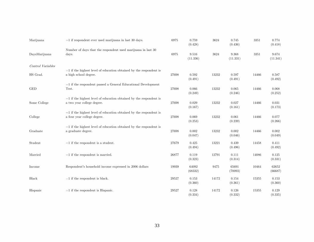
33
Marijuana =1 if respondent ever used marijuana in last 30 days. 6975 0.759 3624 0.745 3351 0.774(0.428) (0.436) (0.418)
DaysMarijuanaNumber of days that the respondent used marijuana in last 30 days. 6975 9.516 3624 9.368 3351 9.674
(11.336) (11.331) (11.341)
Control Variables
HS Grad.=1 if the highest level of education obtained by the respondent is a high school degree. 27698 0.592 13232 0.597 14466 0.587
(0.491) (0.491) (0.492)
GED=1 if the respondent passed a General Educational Development Test. 27698 0.066 13232 0.065 14466 0.068
(0.249) (0.246) (0.252)
Some College=1 if the highest level of education obtained by the respondent is a two year college degree. 27698 0.029 13232 0.027 14466 0.031
(0.167) (0.161) (0.173)
College=1 if the highest level of education obtained by the respondent is a four year college degree. 27698 0.069 13232 0.061 14466 0.077
(0.253) (0.239) (0.266)
Graduate=1 if the highest level of education obtained by the respondent is a graduate degree. 27698 0.002 13232 0.002 14466 0.002
(0.047) (0.046) (0.049)
Student =1 if the respondent is a student. 27679 0.425 13221 0.439 14458 0.411(0.494) (0.496) (0.492)
Married =1 if the respondent is married. 26877 0.119 12791 0.111 14086 0.125(0.323) (0.314) (0.331)
Income Respondent's household income expressed in 2006 dollars 19939 64092 9475 65691 10464 62652(68332) (70093) (66687)
Black =1 if the respondent is black. 29527 0.153 14172 0.154 15355 0.153(0.360) (0.361) (0.360)
Hispanic =1 if the respondent is Hispanic. 29527 0.128 14172 0.126 15355 0.129(0.334) (0.332) (0.335)
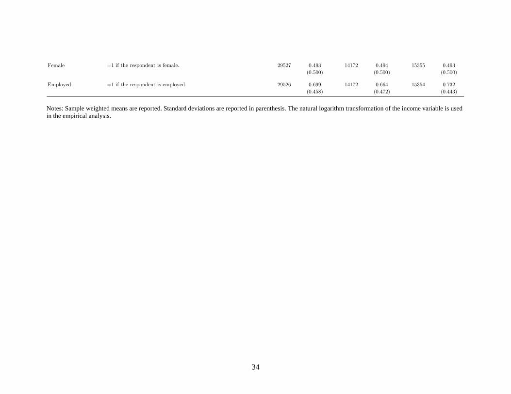
34
Female =1 if the respondent is female. 29527 0.493 14172 0.494 15355 0.493(0.500) (0.500) (0.500)
Employed =1 if the respondent is employed. 29526 0.699 14172 0.664 15354 0.732(0.458) (0.472) (0.443)
Notes: Sample weighted means are reported. Standard deviations are reported in parenthesis. The natural logarithm transformation of the income variable is used in the empirical analysis.

35
Appendix B. Distribution of the number of observations around age 21
500
550
600
650
700
Num
ber o
f obs
.
-24 -12 0 12 24Number of months before or after the 21st birthday
Notes: Total number of observations for each 30-day period around age 21 is plotted. Those who are interviewed on their 21st birthday (15 observations) are not plotted in this graph.
Top Related