THE IDEAL POPULATION: HARDY-WEINBERG EQUILIBRIUM (HWE)

Populations are dynamic groups, that change over space and time. Over succeeding generations, we expect populations to change due to

•!genetic forces •!ecological forces •!evolutionary forces

As population geneticists, we are interested in modeling this change.

A null population is needed to compare empirical and theoretical findings against.

We thus define an ideal population, where NOTHING happens

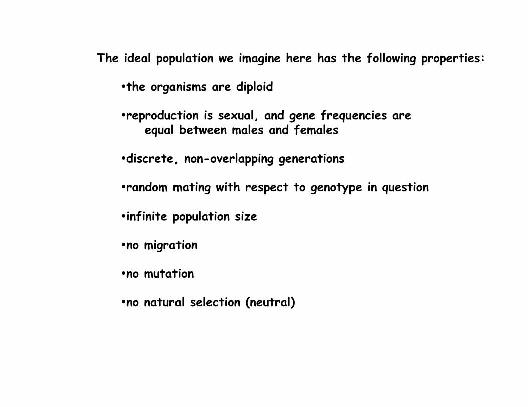
The ideal population we imagine here has the following properties:

•!the organisms are diploid

•!reproduction is sexual, and gene frequencies are equal between males and females

•!discrete, non-overlapping generations

•!random mating with respect to genotype in question

•!infinite population size

•!no migration

•!no mutation

•!no natural selection (neutral)

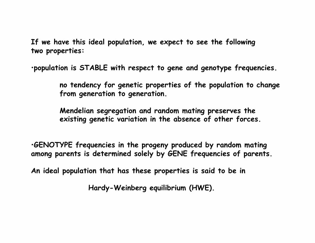
If we have this ideal population, we expect to see the following two properties:

•!population is STABLE with respect to gene and genotype frequencies.

no tendency for genetic properties of the population to change from generation to generation.

Mendelian segregation and random mating preserves the existing genetic variation in the absence of other forces.

•!GENOTYPE frequencies in the progeny produced by random mating among parents is determined solely by GENE frequencies of parents.

An ideal population that has these properties is said to be in

Hardy-Weinberg equilibrium (HWE).

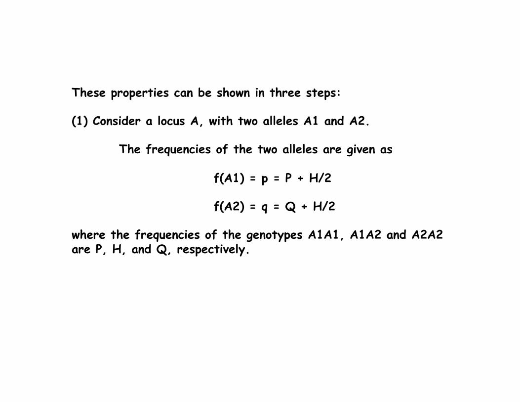
These properties can be shown in three steps:

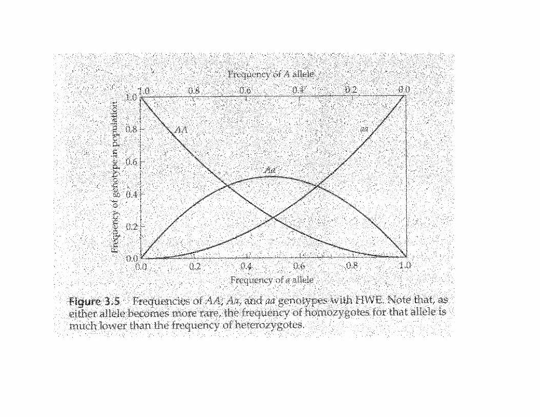
(1) Consider a locus A, with two alleles A1 and A2.

The frequencies of the two alleles are given as

f(A1) = p = P + H/2 f(A2) = q = Q + H/2

where the frequencies of the genotypes A1A1, A1A2 and A2A2 are P, H, and Q, respectively.

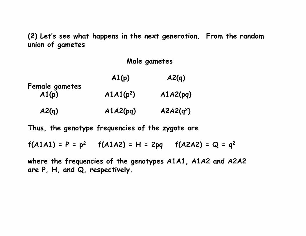
(2) Let’s see what happens in the next generation. From the random union of gametes

Male gametes

A1(p) A2(q) Female gametes A1(p) A1A1(p2) A1A2(pq)

A2(q) A1A2(pq) A2A2(q2)

Thus, the genotype frequencies of the zygote are

f(A1A1) = P = p2 f(A1A2) = H = 2pq f(A2A2) = Q = q2

where the frequencies of the genotypes A1A1, A1A2 and A2A2 are P, H, and Q, respectively.

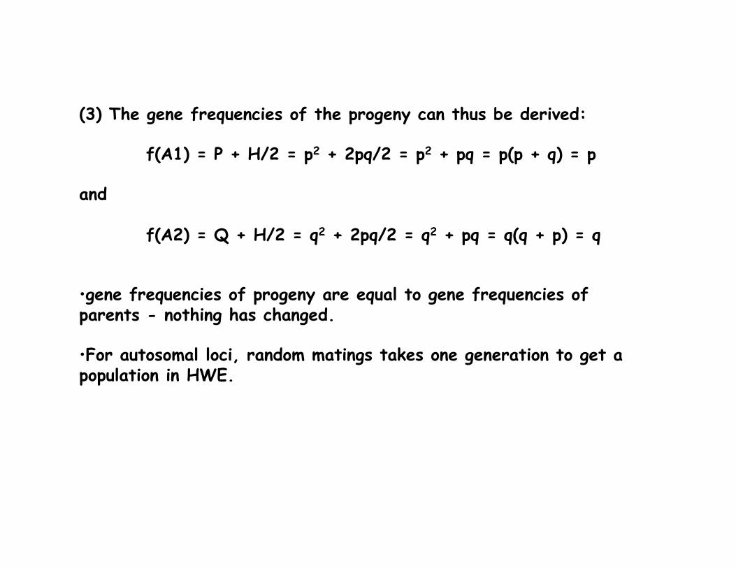
(3) The gene frequencies of the progeny can thus be derived:

f(A1) = P + H/2 = p2 + 2pq/2 = p2 + pq = p(p + q) = p

and

f(A2) = Q + H/2 = q2 + 2pq/2 = q2 + pq = q(q + p) = q

•!gene frequencies of progeny are equal to gene frequencies of parents - nothing has changed.

•!For autosomal loci, random matings takes one generation to get a population in HWE.

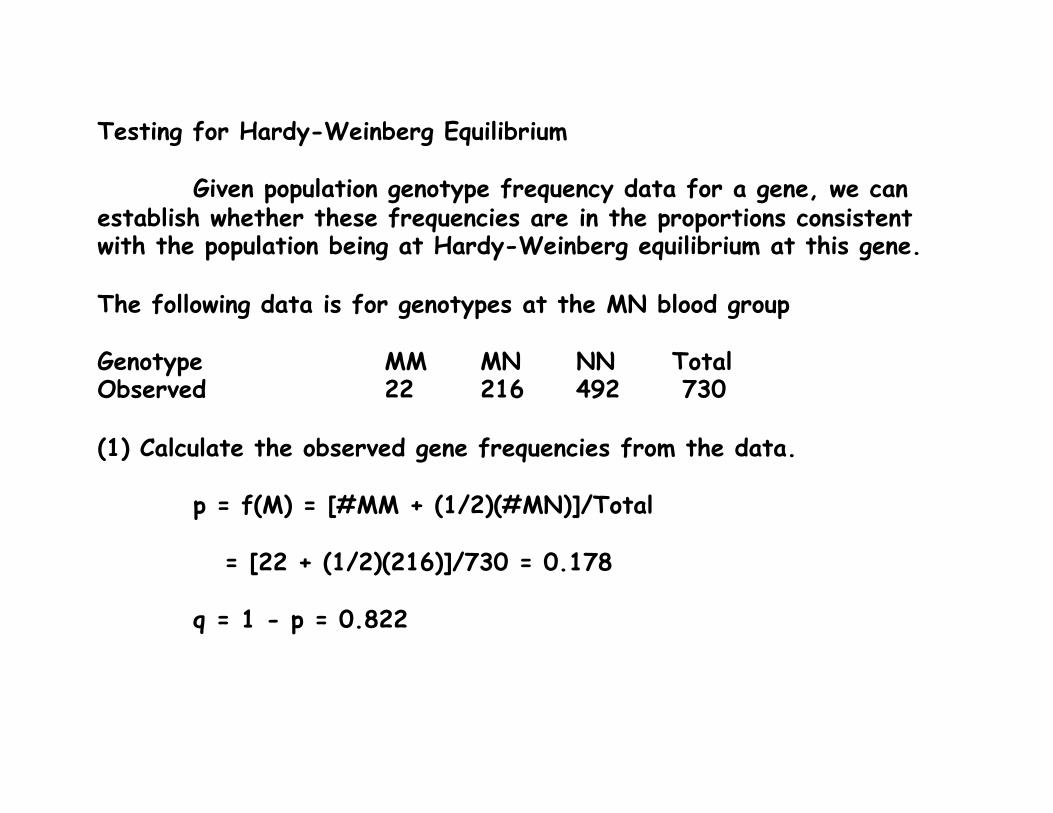
Testing for Hardy-Weinberg Equilibrium

Given population genotype frequency data for a gene, we can establish whether these frequencies are in the proportions consistent with the population being at Hardy-Weinberg equilibrium at this gene.

The following data is for genotypes at the MN blood group

Genotype MM MN NN Total Observed 22 216 492 730

(1) Calculate the observed gene frequencies from the data.

p = f(M) = [#MM + (1/2)(#MN)]/Total

= [22 + (1/2)(216)]/730 = 0.178

q = 1 - p = 0.822

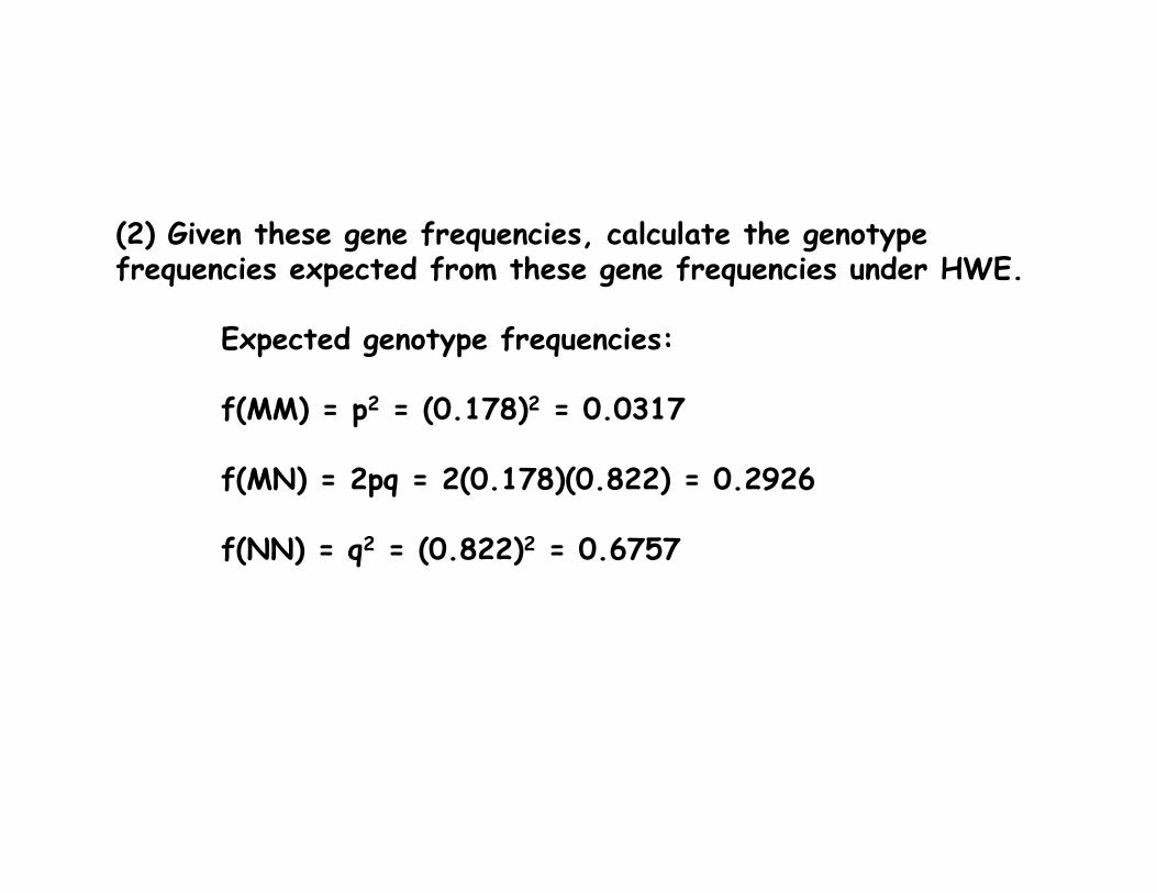
(2) Given these gene frequencies, calculate the genotype frequencies expected from these gene frequencies under HWE.

Expected genotype frequencies:

f(MM) = p2 = (0.178)2 = 0.0317

f(MN) = 2pq = 2(0.178)(0.822) = 0.2926

f(NN) = q2 = (0.822)2 = 0.6757

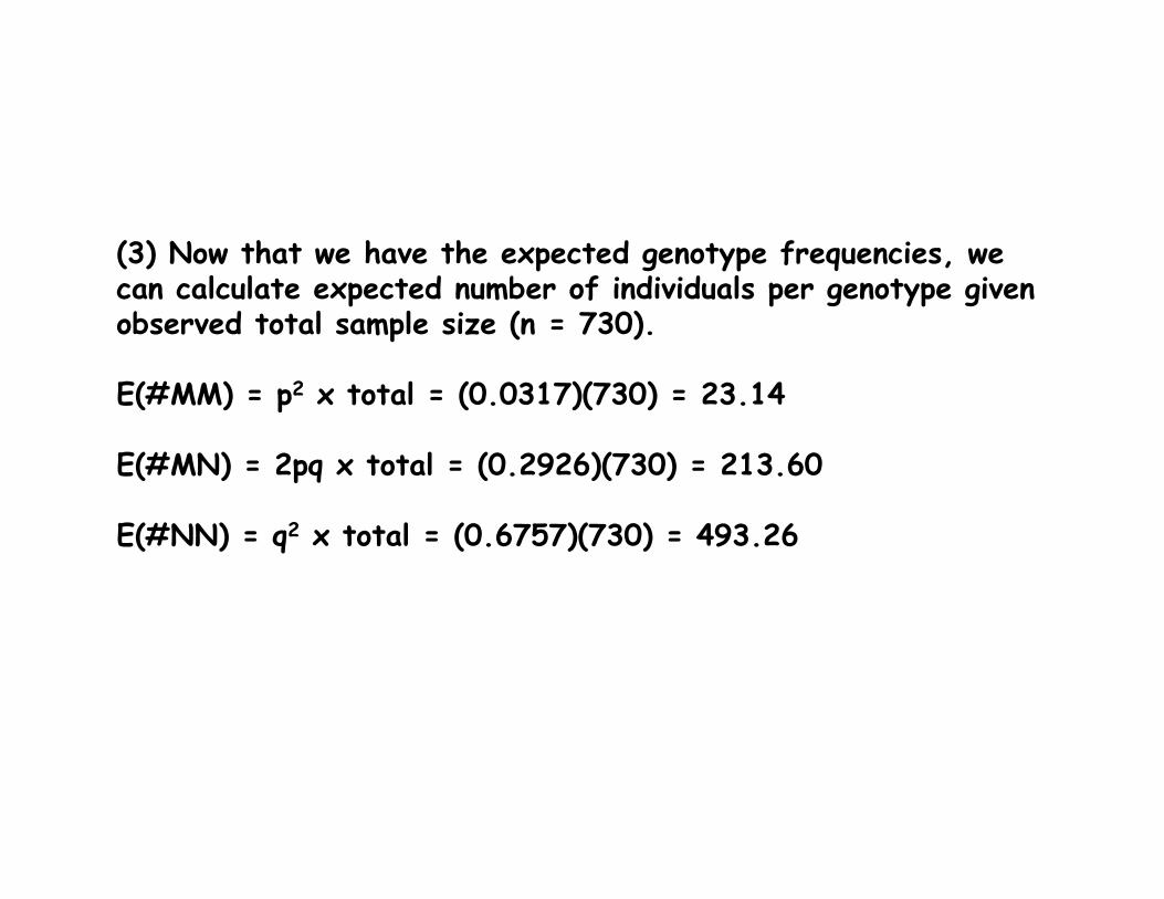
(3) Now that we have the expected genotype frequencies, we can calculate expected number of individuals per genotype given observed total sample size (n = 730).

E(#MM) = p2 x total = (0.0317)(730) = 23.14

E(#MN) = 2pq x total = (0.2926)(730) = 213.60

E(#NN) = q2 x total = (0.6757)(730) = 493.26

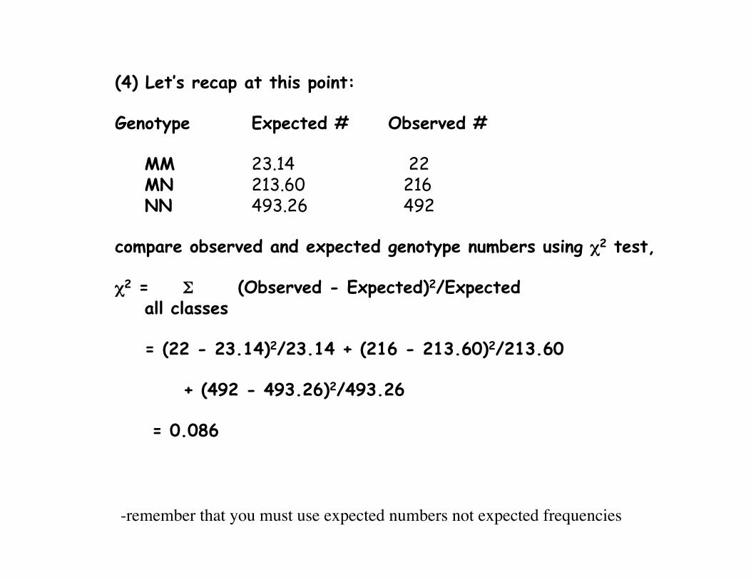
(4) Let’s recap at this point:

Genotype Expected # Observed # MM 23.14 22 MN 213.60 216 NN 493.26 492

compare observed and expected genotype numbers using !2 test,

!2 = " (Observed - Expected)2/Expected all classes

= (22 - 23.14)2/23.14 + (216 - 213.60)2/213.60

+ (492 - 493.26)2/493.26

= 0.086

-remember that you must use expected numbers not expected frequencies!

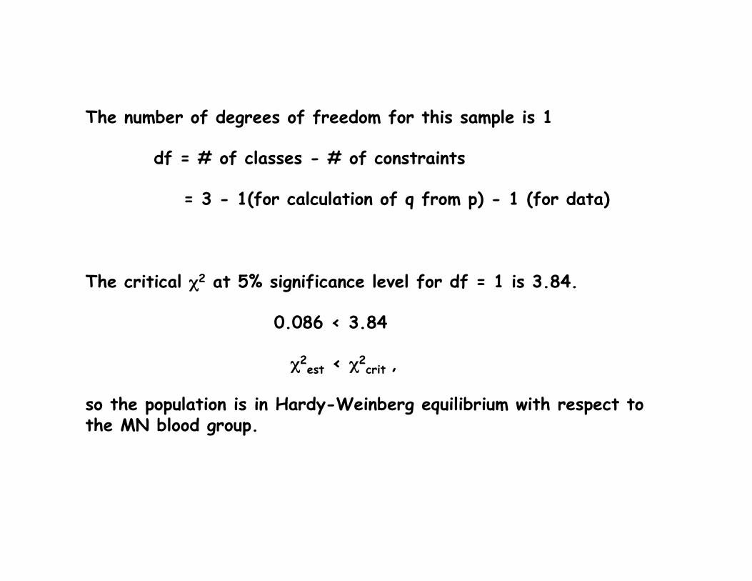
The number of degrees of freedom for this sample is 1

df = # of classes - # of constraints

= 3 - 1(for calculation of q from p) - 1 (for data)

The critical !2 at 5% significance level for df = 1 is 3.84.

0.086 < 3.84

!2est < !

2crit ,

so the population is in Hardy-Weinberg equilibrium with respect to the MN blood group.

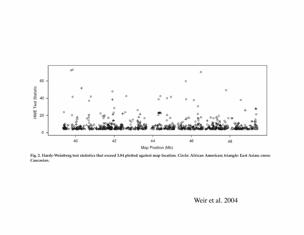
Weir et al. 2004!

Estimating Heterozygote Frequencies for Dominant Alleles

With a dominant allele, we cannot phenotypically distinguish homozygotes from heterozygotes.

Sometimes, though, all we have is visible, phenotypic variation that shows two classes of individuals.

If we assume that the variation is due to a dominant gene and that population is in Hardy-Weinberg equilibrium, then we can calculate frequency of the heterozygotes in the population.

Example: Industrial melanism in the moth Biston betularia

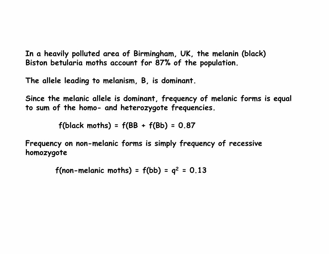
In a heavily polluted area of Birmingham, UK, the melanin (black) Biston betularia moths account for 87% of the population.

The allele leading to melanism, B, is dominant.

Since the melanic allele is dominant, frequency of melanic forms is equal to sum of the homo- and heterozygote frequencies.

f(black moths) = f(BB + f(Bb) = 0.87

Frequency on non-melanic forms is simply frequency of recessive homozygote

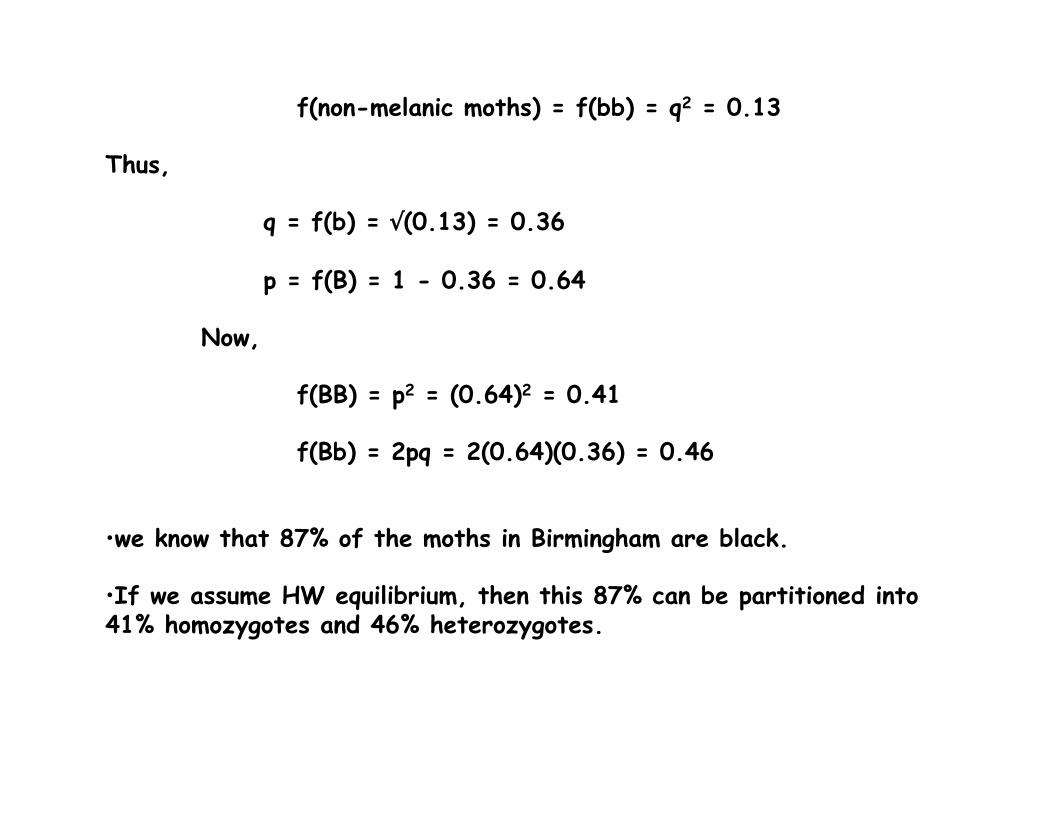
f(non-melanic moths) = f(bb) = q2 = 0.13

f(non-melanic moths) = f(bb) = q2 = 0.13

Thus,

q = f(b) = #(0.13) = 0.36

p = f(B) = 1 - 0.36 = 0.64

Now,

f(BB) = p2 = (0.64)2 = 0.41

f(Bb) = 2pq = 2(0.64)(0.36) = 0.46

•!we know that 87% of the moths in Birmingham are black.

•!If we assume HW equilibrium, then this 87% can be partitioned into 41% homozygotes and 46% heterozygotes.

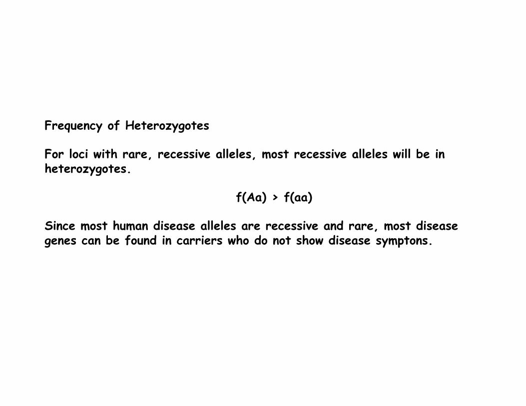
Frequency of Heterozygotes

For loci with rare, recessive alleles, most recessive alleles will be in heterozygotes.

f(Aa) > f(aa)

Since most human disease alleles are recessive and rare, most disease genes can be found in carriers who do not show disease symptons.

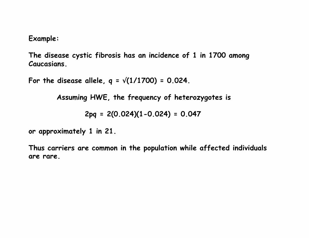
Example:

The disease cystic fibrosis has an incidence of 1 in 1700 among Caucasians.

For the disease allele, q = #(1/1700) = 0.024.

Assuming HWE, the frequency of heterozygotes is

2pq = 2(0.024)(1-0.024) = 0.047

or approximately 1 in 21.

Thus carriers are common in the population while affected individuals are rare.

•!It has been calculated that humans are heterozygous for ~7-8 deleterious recessive alleles.

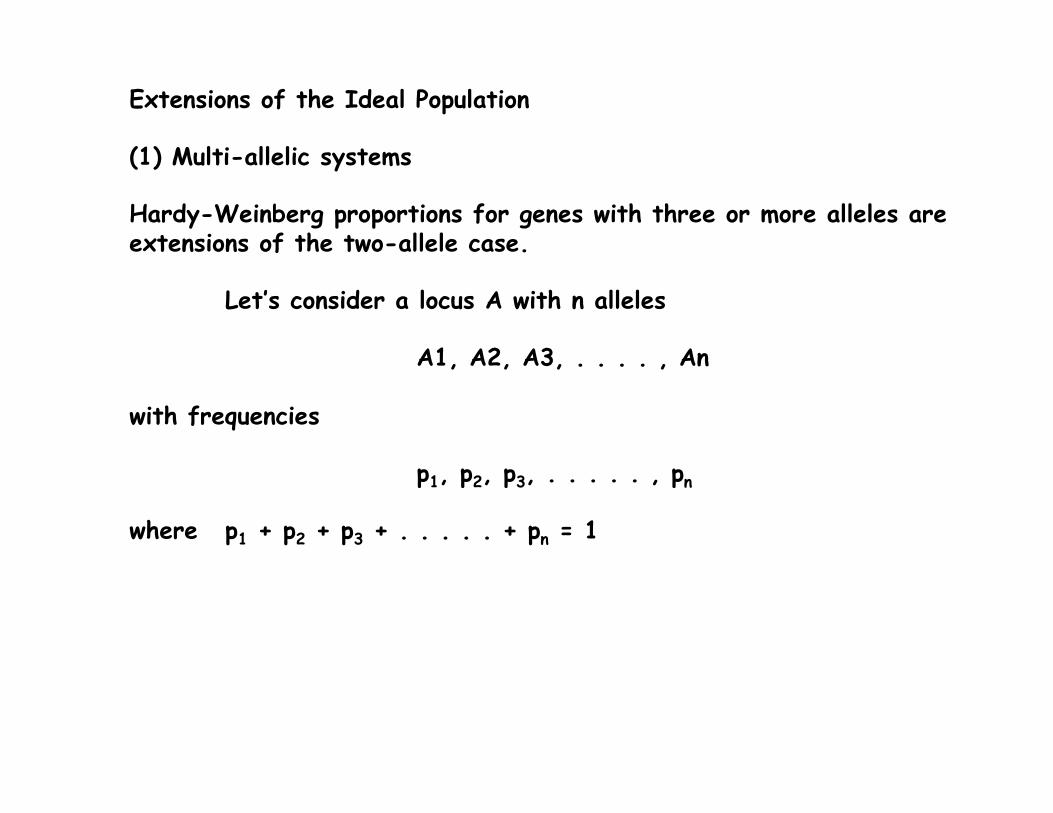
Extensions of the Ideal Population

(1) Multi-allelic systems Hardy-Weinberg proportions for genes with three or more alleles are extensions of the two-allele case.

Let’s consider a locus A with n alleles

A1, A2, A3, . . . . , An

with frequencies

p1, p2, p3, . . . . . , pn

where p1 + p2 + p3 + . . . . . + pn = 1

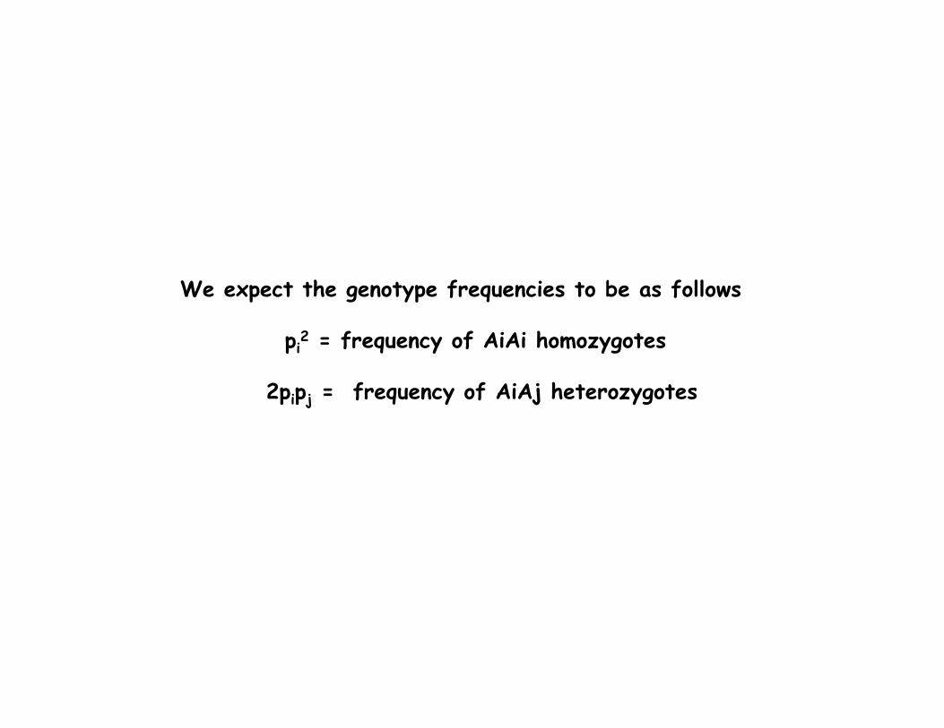
We expect the genotype frequencies to be as follows

pi2 = frequency of AiAi homozygotes

2pipj = frequency of AiAj heterozygotes

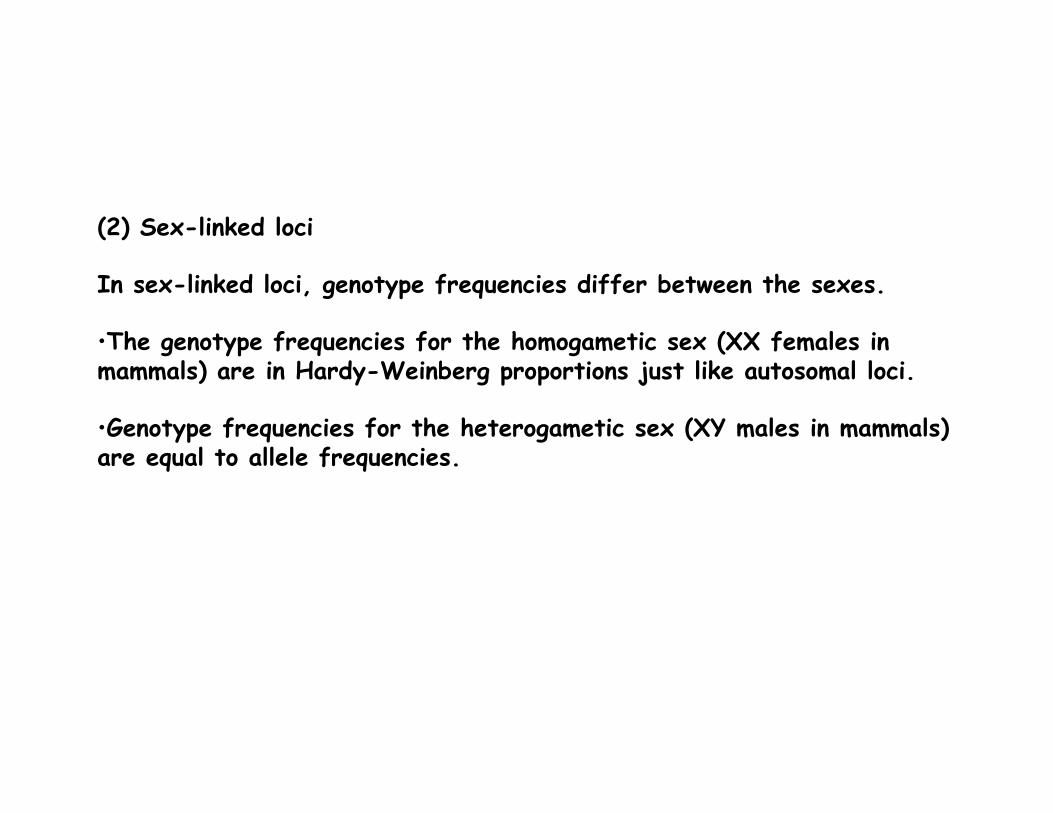
(2) Sex-linked loci

In sex-linked loci, genotype frequencies differ between the sexes.

•!The genotype frequencies for the homogametic sex (XX females in mammals) are in Hardy-Weinberg proportions just like autosomal loci.

•!Genotype frequencies for the heterogametic sex (XY males in mammals) are equal to allele frequencies.

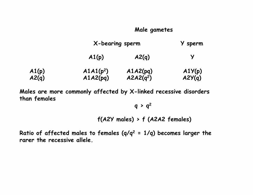
Male gametes

X-bearing sperm Y sperm

A1(p) A2(q) Y

A1(p) A1A1(p2) A1A2(pq) A1Y(p) A2(q) A1A2(pq) A2A2(q2) A2Y(q)

Males are more commonly affected by X-linked recessive disorders than females q > q2

f(A2Y males) > f (A2A2 females)

Ratio of affected males to females (q/q2 = 1/q) becomes larger the rarer the recessive allele.

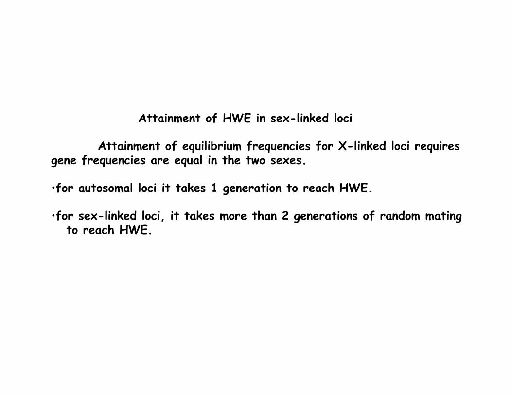
Attainment of HWE in sex-linked loci

Attainment of equilibrium frequencies for X-linked loci requires gene frequencies are equal in the two sexes.

•!for autosomal loci it takes 1 generation to reach HWE.

•!for sex-linked loci, it takes more than 2 generations of random mating to reach HWE.

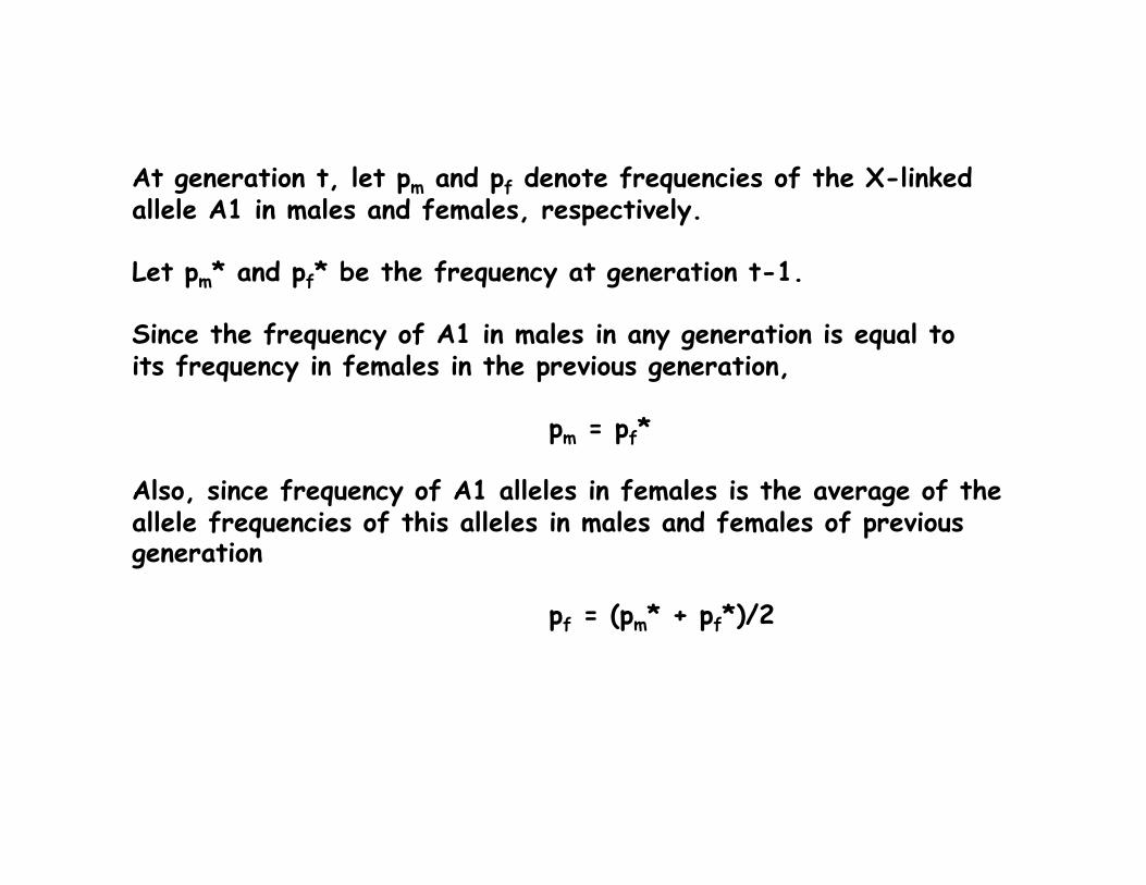
At generation t, let pm and pf denote frequencies of the X-linked allele A1 in males and females, respectively.

Let pm* and pf* be the frequency at generation t-1.

Since the frequency of A1 in males in any generation is equal to its frequency in females in the previous generation,

pm = pf*

Also, since frequency of A1 alleles in females is the average of the allele frequencies of this alleles in males and females of previous generation

pf = (pm* + pf*)/2

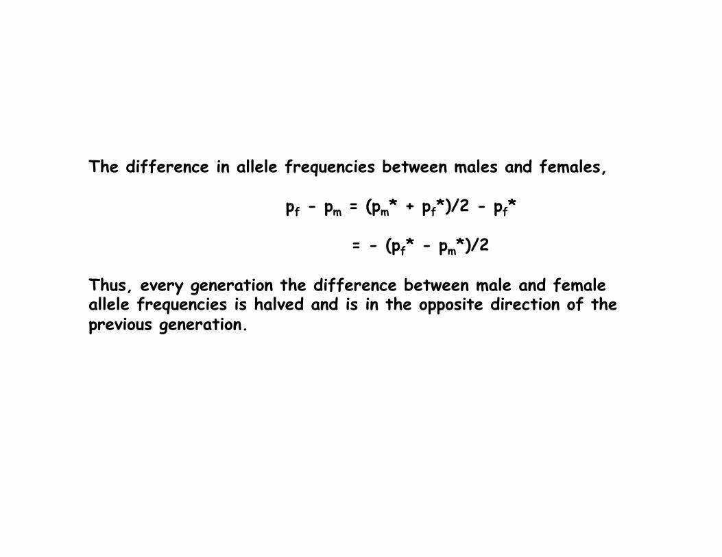
The difference in allele frequencies between males and females,

pf - pm = (pm* + pf*)/2 - pf*

= - (pf* - pm*)/2

Thus, every generation the difference between male and female allele frequencies is halved and is in the opposite direction of the previous generation.