


Languages
Pages
Legal

The Cyclical Response of Advertising Refutes Countercyclical
Profit Margins in Favor of Product-Market Frictions ∗
Robert E. HallHoover Institution and Department of Economics,
Stanford UniversityNational Bureau of Economic [email protected]; website: Google “Bob Hall”
November 2, 2012
Abstract
According to the standard model, advertising is remarkably sensitive to profit mar-gins. Firms advertise to stimulate demand for their products. They advertise high-margin products aggressively and low-margin ones hardly at all. In macroeconomics,variations in profit margins over the business cycle have a key role. A widening ofmargins can explain the rise in unemployment in recessions. A higher margin implies alower real wage. A variety of models ranging from Keynesian to search-and-matchingmap a decline in wages to higher unemployment. But a rise in profit margins shouldexpand advertising by a lot. Really a lot. Advertising should be highly countercyclical.Instead, it is somewhat procyclical. The ratio of advertising spending to private GDPfalls when the economy contracts. The behavior of advertising refutes the hypothesisthat profit margins rise. But it is true that the labor share of income falls. Hence theremust be another factor that lowers the labor share without raising profit margins. Theonly influence that fits the facts is a rise in a product-market friction that has the sameeffect as an increase in sales taxes.
JEL D43 E12 E32
∗The Hoover Institution supported this research. The research is also part of the National Bureau ofEconomic Research’s Economic Fluctuations and Growth Program. I am grateful to Kyle Bagwell, MarkBils, Valerie Ramey, Julio Rotemberg, Stephen Sun, and Michael Woodford for valuable comments.
1

Theorem: Let R be the ratio of advertising expenditure to the value of output.
Let −ε be the residual elasticity of demand. Let m be an exogenous shift in the
profit margin. Then the elasticity of R with respect to m is ε − 1, which is a
really big number.
After proving this theorem, which is a direct implication of the standard model of ad-
vertising, I dwell on its implications for an important issue in macroeconomics, the role of
shifts in the profit margin. The basic idea is simple. In a slump, firms do not cut prices
in answer to disappointing sales. If their costs are lower—because they have moved down
their upward-sloping short-run marginal costs curves or because flexible-price factor markets
now have lower prices—their profit margins are higher. The theorem says that they should
expand advertising by substantial amounts. Consider the middle-of-the-road value for the
typical residual elasticity of demand of 6, so that the ratio of price over marginal cost is 6/(6-
1) = 1.2 The ratio of advertising spending to GDP should rise by 5 times the proportional
increase in that ratio. Advertising should be highly countercyclical. Firms should expand
advertising aggressively in a slump.
In fact, advertising is procyclical. I show that the ratio of advertising to GDP falls by
about one percent for each percentage point of extra unemployment. Far from boosting
advertising to recover business lost in a slump, firms cut advertising by even more than their
loss of sales. The key finding, however, is that advertising is not highly countercyclical. I
would have written this paper even if I had found advertising to be noncyclical or mildly
countercyclical.
The thrust of standard advertising theory is that advertising should rise and fall in
proportion to sales. The formula for the ratio is remarkably simple; it is the elasticity of
sales with respect to advertising effort divided by the residual elasticity of demand. If the
two elasticities are constants not influenced by the factors causing a slump, then advertising
will be a constant fraction of sales. Macroeconomics has brought into play a mechanism not
usually considered in advertising theory, namely that profit margins widen in slumps. That
widening should result in a splurge of advertising in slumps.
The question at this point is what other factor could be operating to alter the standard
property that implies that advertising should be neither procyclical (as it actually is) nor
countercyclical (as the widening-margin model implies). In my baseline model, I include a
friction that has the effect on a firm that a sales tax would. I call this a product-market fric-
2
tion. I use the term wedge to describe the shift in the profit margin and the product-market
friction. This term is widely used in macroeconomics to describe variables that measure
gaps between theoretical first-order conditions and the actual values of the corresponding
variables.
The paper studies two key observed variables: (1) the ratio of advertising spending to
revenue, and (2) the ratio of labor compensation to revenue (the labor share). Both the profit-
margin wedge and the product-market friction wedge affect these variables. The elasticity
of the advertising ratio with respect to the profit-margin wedge is ε− 1, a number around 5.
The elasticities of the advertising ratio with respect to the product-market friction wedge and
of the labor share with respect to both wedges are all −1. The fact that the profit-margin
wedge has a large effect on the advertising ratio has a neat implication. Consider the ratio
of the advertising/sales variable to the labor share. One fact is that the elasticity of that
ratio with respect to the product-market friction is zero, because the friction has the same
effect on numerator and denominator. The second fact is that the elasticity of the ratio with
respect to the profit-margin wedge is the residual elasticity of demand, ε, say 6. These facts
provide a clean identification of the role of the profit-margin wedge. That wedge should have
a big positive effect on advertising in recessions, under the view that profit margins increase
in recessions. A regression of the ratio of the advertising/sales variable to the labor share
on employment should have a big negative coefficient that arises entirely from the margin
effect and not at all from the product-market friction. In reality, the regression coefficient is
slightly positive and the confidence interval around it excludes any big negative effect. The
finding casts serious doubt on the countercyclical profit-margin hypothesis
On the other hand, the product-market friction emerges as a fully consistent idea about
the character of slumps. It says that rising frictions in recessions lower advertising and the
labor share about equally, leaving the ratio of the two variables close to noncyclical. I avoid
speculation in this paper about the nature of the friction.
I consider a number of potential variations around the basic specification in the paper.
The first is to follow an important branch of the advertising literature and treat advertising
expenditure as a form of investment. Because investment in, say, plant and equipment is quite
procyclical, this consideration might explain the findings despite a countercyclical margin—
the procyclical effect from investment might be swamping the large countercyclical effect of
the margin changes. But a reformulation of the model using standard investment theory
3

shows otherwise. A key factor in this finding is the high depreciation rate of advertising.
A consensus of research on advertising is that around 60 percent of the effect of earlier
advertising dissipates each year.
I also consider a model extended to include other cyclical shifts. These are (1) changes in
productivity, (2) measurement error in the labor share, (3) measurement error in the capital
share, and (4) measurement error in the price of advertising. I show that productivity and
capital measurement errors have no effect on the measured values of the variables I study.
Of course, they do affect other variables—the point is that they drop out of the ratios I
consider. A plausible measurement error in the labor share—an idea I take seriously—goes
in the wrong direction to overcome the findings. Measurement error in the price of advertising
could conceal part of its countercyclical movements but would have to be implausibly large
to overturn the basic conclusion of the paper. The most likely form of such an error would
come from failing to consider the investment component of advertising, a topic I consider
separately with negative conclusions.
1 Related Research
1.1 Cyclical behavior of advertising
Borden (1942) noted the close correlation between advertising volume and an index of indus-
trial production—see Simon (1970), Figures 2-11 and 2-12, who also cites a number of other
sources confirming the correlation. Kaldor (1950) noted a similar correlation and Blank
(1962) and Yang (1964) documented the correlation, without theoretical interpretation. Bils
(1989), Table 1, presents regressions of the rate of change of real advertising expenditures
on the rate of change of real GDP. A coefficient greater than one would indicate procyclical
movements as that term is used in this paper. He uses data for the U.S. and Britain. In all
cases the coefficients are positive and for more recent U.S. data and all British data, they
exceed one. The model in the paper implies countercyclical market power for reasons similar
to Edmond and Veldkamp (2009), discussed below, but Bils interprets the model as pointing
toward procyclical advertising.
1.2 The level of market power
Positive advertising expenditure proves the existence of market power, for there is no incen-
tive to advertise in perfectly competitive markets. Still, there is remarkably little consensus
4

on the extent of market power in the U.S. economy. The most recent survey of the subject
appears to be Bresnahan (1989). His summary, in Table 17.1, reports residual elasticities in
the range from 1.14 to 40, for industries from coffee roasting to banking. Many subsequent
studies, mainly for consumer packaged goods, have appeared since the publication of Bres-
nahan’s survey. I am not aware of any attempt to distill a national average from studies
for individual products. Hausman, Leonard and Zona (1994), for example, study the de-
mand for beer and find residual elasticities (holding the prices of competing beers constant)
in the range from 3.5 to 5.9. Most research does not try to reconcile residual elasticities
estimated from demand equations with data on price/marginal cost ratios from producers,
though Bresnahan discusses this topic extensively. De Loecker and Warzynski (2012) use
firm-level from Slovenia in a producer-side framework and find average markups of about
1.2, corresponding to a residual elasticity of demand of 6, the value I take in my base case.
1.3 Cyclical changes in market power
Macroeconomics has spawned a large literature on countercyclical market power. Bils (1987)
launched the modern literature that studies cyclical variation in the labor share. My inter-
pretation of that literature is that it measures not variations in profit margins but rather in
the labor share, because these are not the same thing in the presence of the product-market
friction that I consider. Bils made important adjustments based on cyclical variations in the
incidence of overtime wages. Rotemberg and Woodford (1999) embraced Bils’s adjustments
in a survey chapter that explains how New Keynesian models explain cyclical variations
in output and employment through variations in market power resulting from sticky prices
and flexible cost. Nekarda and Ramey (2010) and Nekarda and Ramey (2011) challenge the
findings of countercyclical market power in favor of cyclically constant markups resulting
from Bils’s overstatement of the incidence and magnitude of overtime premiums.
Bils and Kahn (2000) argue that marginal cost is procyclical because firms internalize
the fluctuations in their employees’ disamenity of work effort. In slumps, the marginal
disamenity of effort is low, because effort itself is low. In an expansion, as effort rises, its
marginal burden on workers rises and marginal cost of production rises accordingly, even
if cash payments to workers do not rise in proportion to the marginal burden. They use
this hypothesis to explain the otherwise puzzling behavior of inventory investment. Firms
allow inventory levels to decline persistently below normal during booms and above normal
5

in slumps, which would only make sense if marginal production costs are high in booms and
low in slumps.
Chevalier and Scharfstein (1996) develop and estimate a model in which capital-market
frictions influence pricing decisions at the retail level. In slumps, firms that are financially
constrained disinvest in customers by setting prices at higher than normal margins over
marginal cost.
Edmond and Veldkamp (2009) look at the issues of market power from the consumer’s
perspective. They find that rising dispersion of income distribution lowers residual elasticities
in slumps. Firms respond by setting prices further above marginal cost.
The literature on cyclical changes in market power is complementary to the ideas in this
paper. In many of the accounts in the existing literature, the question becomes acute: Why
does advertising not expand in slumps when the residual elasticity falls?
1.4 Cyclical fluctuations in product-market friction
I am not aware of any work on this topic.
2 Theory
Suppose that the residual demand facing a firm is a constant-elastic function of the firm’s
price p, the average p of its rivals’ prices, its own advertising A, and the average of its rivals’
advertising A, with elasticities −ε, ε, α, and −α. The marginal cost of production is c and
the cost of a unit of advertising is κ. Although customers pay p for each unit of output,
the firm receives only p/f , where f is a product-market friction or wedge that depresses the
price the firm receives. The factor f may be above or below 1. The firm’s objective is
maxp,A
(p
f− c
)p−ε p εAαA −α − κA. (1)
The profit-maximizing price is
p∗ =ε
ε− 1f c (2)
and in symmetric equilibrium, p = p and A = A. For some reason—possibly price stickiness—
the firm actually sets the price
p = m p∗. (3)
6

The profit-margin wedge, m, may be above or below 1. If m > 1, the firm keeps the added
profit per unit sold though it loses profit overall from the reduced volume. The reverse occurs
if m < 1.
Equation (2) and equation (13) imply
p = m fε
ε− 1c. (4)
The variable part of the markup of price p over marginal cost c is the product of the two
wedges, mf . The profit-margin wedge has implications stressed in Rotemberg and Woodford
(1999) and is the way that sticky prices affect real allocations, as those authors explain. On
the other hand, the friction f also appears in equation (1), where it has the effect of taking
away the margin increase from the firm, so an increase in f does not raise profit. Conse-
quently, the two wedges have quite different effects. Later in the paper I will demonstrate
that authors thinking they are measuring the profit-margin wedge m by studying labor’s
share of total cost are actually measuring the compound wedge mf , under the assumptions
of this model.
2.1 Advertising
The first-order condition for advertising is
α
AQ
(p
f− c
)= κ. (5)
Rearranging and dividing both sides by p yields an expression for the ratio of advertising
expenditure to revenue:κA
pQ= α
p/f − cp
. (6)
Substituting for p from equation (13) and for p∗ from equation (2) restates the right-hand
side in terms of exogenous influences:
R =κA
pQ= α
(m− 1)ε+ 1
f m ε(7)
Absent the special influences captured by f and m, that is, with f = m = 1, the advertis-
ing/revenue ratio is
R =α
ε, (8)
a standard result in the advertising literature, first derived by Dorfman and Steiner (1954).
See Bagwell (2007) for an impressively complete review of the literature on the economics of
advertising.
7

From these equations, two useful results follow:
Proposition Rm: The elasticity of the advertising ratio R with respect to the profit-margin
shockwedge m at the point f = m = 1 is ε− 1.
Proposition Rf: The elasticity of the advertising ratio with respect to the friction f is −1.
Proposition Rm is the centerpiece of the paper—advertising is highly sensitive to the
profit-margin wedge. If markups rise in a slump, firms should increase efforts aggressively
to attract new customers and retain existing ones, because selling to them has become more
profitable.
2.2 Labor share
The second measure is the labor share
λ =W
pQ. (9)
Here W is the firm’s total wage bill including all forms of compensation. Under the assump-
tions of Cobb-Douglas technology with labor elasticity γ and cost minimization, the wage
bill is γ c Q, so
λ =γ c Q
pQ= γ
ε− 1
ε
1
f m(10)
Two additional results then follow immediately:
Proposition λm: The elasticity of the labor share λ with respect to the profit-margin
wedge m is −1.
Proposition λf: The elasticity of the labor share with respect to the product-market wedge
f is −1.
2.3 Solving for the wedges
From the propositions above,
logR = (ε− 1) logm− log f + µR (11)
and
log λ = − logm− log f + µλ, (12)
where µR and µλ are constant and slow-moving influences apart from m and f .
8

Solving this pair of equations for logm and log f yields
logm =logR− log λ
ε+ µm (13)
and
log f = − log λ− logR− log λ
ε+ µf . (14)
Here µm and µf are constant and slow-moving influences derived in the obvious way from
µR and µλ.
2.4 The role of cyclical movements
The main goal of this paper is to study movements of the observed time series R and λ and
make inferences about the cyclical movements of the inferred wedges m and f , especially
to quantify their contributions to the business cycle. Throughout the paper, I measure
the business cycle by the employment rate, the fraction of the labor force holding jobs
(one minus the unemployment rate). Variables are procyclical if they move positively with
the employment rate and countercyclical if they move negatively. The data show that the
advertising/sales ratio R and the labor share λ are quite procyclical. The expectation is
that the wedges are both countercyclical—they measure forces that cause reductions in
employment when they rise.
3 Cyclical Movements of Advertising/GDP Ratio and
the Labor Share
For many years, Robert J. Coen of the ad agency Erickson-McCann published a compilation
of data on advertising expenditure. I was unable to find any surviving original copy of his
data. Douglas Galbi posted a copy of Coen’s estimates through 2007 in his blog, along with
estimates for early years from other sources. Galbi also provides links to Coen’s data sources,
but the only one still active is for the data on newspapers. Further information about the
sources appears in the appendix.
For 2005 through 2010, the Census Bureau has published revenue data for NAICS indus-
try 51, the information sector, which includes the advertising industries. I define advertising
as the sum of newspapers, magazines, broadcasting, and Internet. In the three years that
the Census figures overlap Coen’s, the latter is 1.38 times the former. I take the figures for
2008 through 2010 to be this factor times the Census figure.
9
I am continuing to explore alternative data sources for advertising spending, at the ag-
gregate and industry levels. The Internal Revenue Service publishes data for corporate
advertising deductions for recent years and possibly for earlier years, but only on paper.
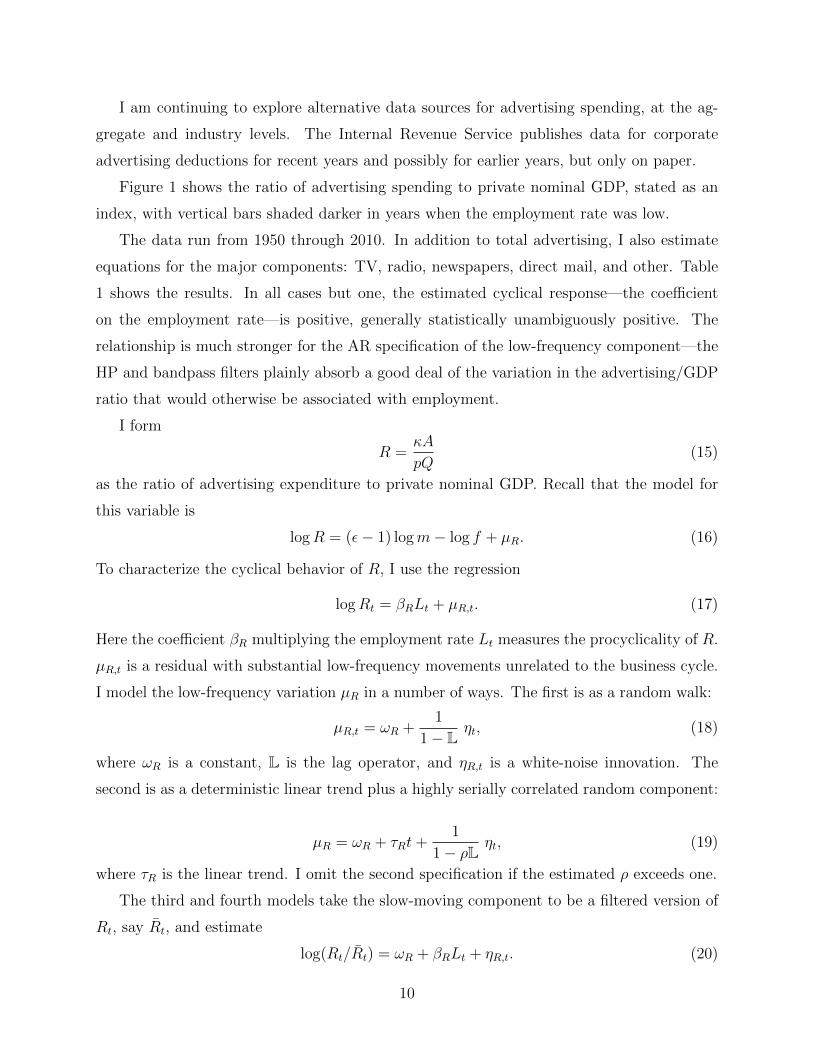
Figure 1 shows the ratio of advertising spending to private nominal GDP, stated as an
index, with vertical bars shaded darker in years when the employment rate was low.
The data run from 1950 through 2010. In addition to total advertising, I also estimate
equations for the major components: TV, radio, newspapers, direct mail, and other. Table
1 shows the results. In all cases but one, the estimated cyclical response—the coefficient
on the employment rate—is positive, generally statistically unambiguously positive. The
relationship is much stronger for the AR specification of the low-frequency component—the
HP and bandpass filters plainly absorb a good deal of the variation in the advertising/GDP
ratio that would otherwise be associated with employment.
I form
R =κA
pQ(15)
as the ratio of advertising expenditure to private nominal GDP. Recall that the model for
this variable is
logR = (ε− 1) logm− log f + µR. (16)
To characterize the cyclical behavior of R, I use the regression
logRt = βRLt + µR,t. (17)
Here the coefficient βR multiplying the employment rate Lt measures the procyclicality of R.
µR,t is a residual with substantial low-frequency movements unrelated to the business cycle.
I model the low-frequency variation µR in a number of ways. The first is as a random walk:
µR,t = ωR +1
1− Lηt, (18)
where ωR is a constant, L is the lag operator, and ηR,t is a white-noise innovation. The
second is as a deterministic linear trend plus a highly serially correlated random component:
µR = ωR + τRt+1
1− ρLηt, (19)
where τR is the linear trend. I omit the second specification if the estimated ρ exceeds one.
The third and fourth models take the slow-moving component to be a filtered version of
Rt, say Rt, and estimate
log(Rt/Rt) = ωR + βRLt + ηR,t. (20)
10

0.90
0.95
1.00
1.05
1.10
1.15
1.20
0.70
0.75
0.80
0.85
1950
1955
1960
1965
1970
1975
1980
1985
1990
1995
2000
2005
2010
Figure 1: Index of the Ratio of Advertising Spending to Private GDP, with Shading inProportion to the Employment Rate
11

Change in log of all types of advertising/GDP
0.97 (0.37) - - - -
Log of all types of advertising/GDP 0.97 (0.39) 0.000 (0.004) 0.93 (0.05)
HP cycle component 0.41 (0.23) - - - -
Bandpass cycle component 0.36 (0.16) - - - -
TV ads 0.40 (0.71) 0.014 (0.002) 0.71 (0.03)
Radio ads 0.37 (0.55) 0.008 (0.002) 0.81 (0.04)
Newspaper ads 1.19 (0.51) - - - -
Direct mail -0.42 (0.49) 0.011 (0.008) 0.96 (0.04)
Other advertising 1.74 (0.54) -0.011 (0.001) 0.77 (0.08)
Note: The right-hand variable in the first row is in first differences. Regressions include constants, not shown.
Employment rate Trend Autoregressive termLeft-hand variable
Coefficients and standard errors
Table 1: Cyclical Behavior of the Advertising/GDP Ratio
The filter absorbs any trend in Rt, so I do not include an explicit trend. For the filters, I
use Hodrick-Prescott with smoothing parameter 6.25 and a bandpass filter that passes cycle
periods of 2 through 8 years.
The data run from 1950 through 2010. In addition to total advertising, I also estimate
equations for the major components: TV, radio, newspapers, direct mail, and other. Table
1 shows the results. In all cases but one, the estimated cyclical response—the coefficient
on the employment rate—is positive, generally statistically unambiguously positive. The
advertising/GDP ratio is plainly procyclical—it rises when employment rises. The rela-
tionship is much stronger for the random-walk and AR specifications of the low-frequency
component—the HP and bandpass filters plainly absorb a good deal of the variation in the
advertising/GDP ratio that would otherwise be associated with employment.
I reiterate that the finding that advertising is procyclical is not central to the point of the
12
paper. Rather, the key finding is that advertising is not strongly countercyclical, as it would
be if the profit margin were countercyclical. The findings in Table 1 are not dispositive on the
unimportance of fluctuations in the profit margin, however, because there is a possibility that
a strongly procyclical effect from the product-market friction is masking a countercyclical
effect from the margin. To deal with this issue, I turn to a study of the cyclical movement
of the labor share.
4 The Labor Share
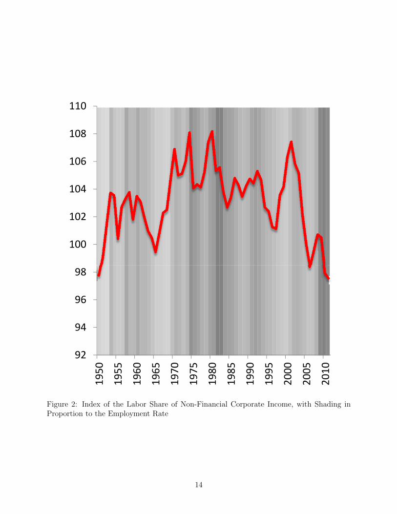
The Bureau of Labor Statistics publishes a quarterly index of the labor share of non-financial
corporations at bls.gov/lpc, series PRS88003173, starting in 1947. The limitation to corpo-
rations is desirable because there is no reliable basis for dividing proprietary income into
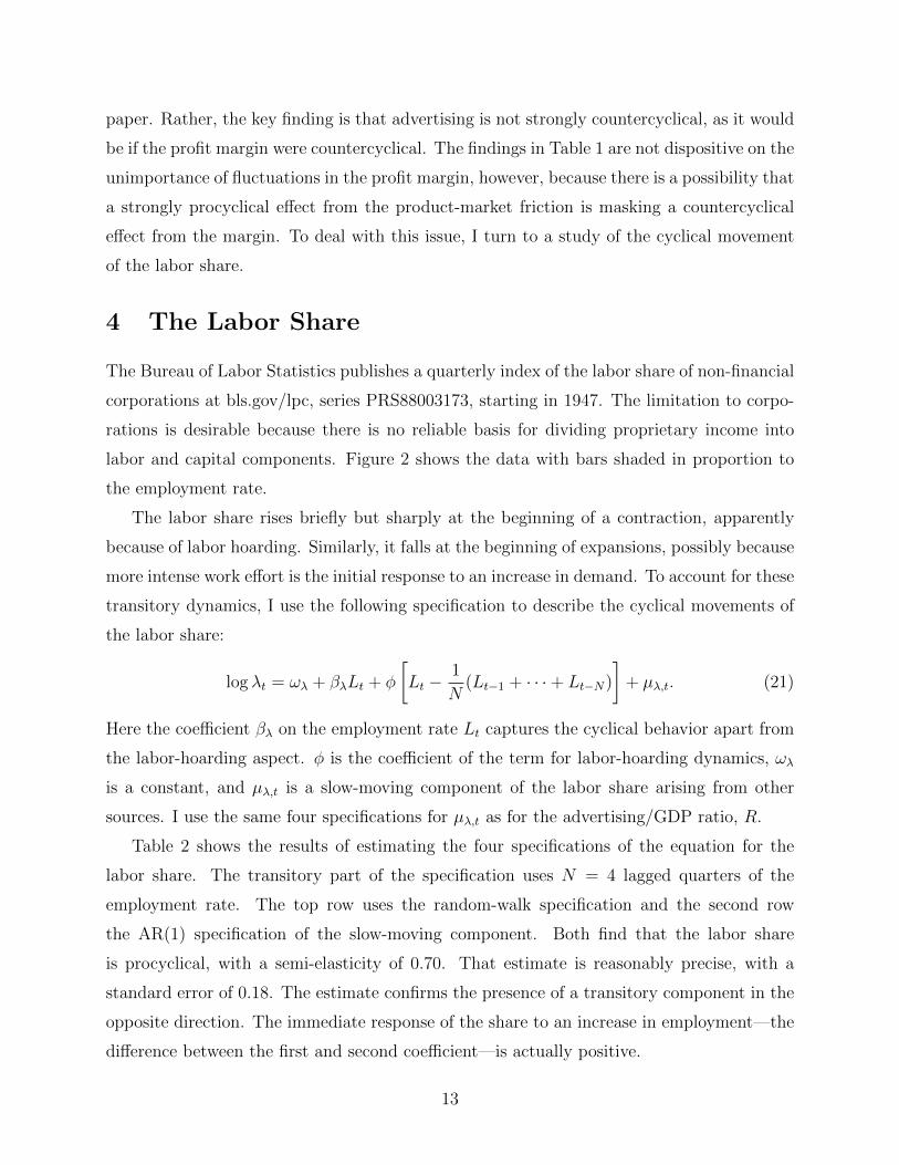
labor and capital components. Figure 2 shows the data with bars shaded in proportion to
the employment rate.
The labor share rises briefly but sharply at the beginning of a contraction, apparently
because of labor hoarding. Similarly, it falls at the beginning of expansions, possibly because
more intense work effort is the initial response to an increase in demand. To account for these
transitory dynamics, I use the following specification to describe the cyclical movements of
the labor share:
log λt = ωλ + βλLt + φ
[Lt −
1
N(Lt−1 + · · ·+ Lt−N)
]+ µλ,t. (21)
Here the coefficient βλ on the employment rate Lt captures the cyclical behavior apart from
the labor-hoarding aspect. φ is the coefficient of the term for labor-hoarding dynamics, ωλ
is a constant, and µλ,t is a slow-moving component of the labor share arising from other
sources. I use the same four specifications for µλ,t as for the advertising/GDP ratio, R.
Table 2 shows the results of estimating the four specifications of the equation for the
labor share. The transitory part of the specification uses N = 4 lagged quarters of the
employment rate. The top row uses the random-walk specification and the second row
the AR(1) specification of the slow-moving component. Both find that the labor share
is procyclical, with a semi-elasticity of 0.70. That estimate is reasonably precise, with a
standard error of 0.18. The estimate confirms the presence of a transitory component in the
opposite direction. The immediate response of the share to an increase in employment—the
difference between the first and second coefficient—is actually positive.
13
100
102
104
106
108
110
92
94
96
98
1950
1955
1960
1965
1970
1975
1980
1985
1990
1995
2000
2005
2010
Figure 2: Index of the Labor Share of Non-Financial Corporate Income, with Shading inProportion to the Employment Rate
14

Change in log labor share 0.70 (0.18) -1.24 (0.17) - -
Log labor share 0.70 (0.18) -1.23 (0.17) 0.957 (0.019)
HP cycle component 0.27 (0.06) -1.39 (0.14) - -
Bandpass cycle component 0.27 (0.06) -1.33 (0.13) - -
Note: The two right-hand variables in the first row are in first differences.
Regressions include constants, not shown
Left-hand variable Departure of employment rate from recent past
Autoregressive termEmployment rate
Coefficients and standard errors
Table 2: Cyclical Behavior of the Labor Share
The third and fourth lines in Table 2 use filtering methods on the share to account for
its slower movements. They find semi-elasticities about half as large. The reported standard
error is probably an overstatement of the reliability, as it does not account for the preliminary
filtering.
I conclude that both the advertising/GDP ratio and the labor share are procyclical. This
finding points strongly in the direction of an influence of the product-market friction that
trumps any influence of the profit-margin wedge, given that the latter would stimulate a
powerful countercyclical response of advertising.
5 The Values of the Wedges and Their Effects on Em-
ployment
The empirical counterparts of the two wedges, including their low-frequency components,
are
logM =logR− log λ
ε(22)
and
logF = − log λ− logR− log λ
ε. (23)
15

Constructing these variables requires a value of the residual elasticity of demand ε. As
I noted earlier, though market power is an important topic in many branches of applied
microeconomics and is the subject of a large literature, the results of empirical research are
inconclusive with respect to any single value for ε that would typify the aggregate economy.
Research has concentrated on packaged consumer goods and thus left most components of
total production untouched. That said, most economists would probably place the typical
value of the residual elasticity of demand in the range from 3 to 20, corresponding to profit
margins of 33 down to 5 percent of price. I will present results for ε = 6, which corresponds
to a markup ratio of ε/(ε− 1) = 1.2, along with a discussion of results for lower and higher
amounts of market power.
Figure 3 and Figure 4 show the values of the two wedges, with slumps marked by dark
bars, again shaded in proportion to the employment rate. The basic findings of the paper
are plainly visible in these figures. Recall from equation (13) that the calculated value of the
profit-margin wedge subtracts the log of the labor share from the log of the advertising/GDP
ratio, which removes the common element of the two. That element is the log of the product-
market friction, log f . What is left has almost no cyclical movement. On the other hand,
log f , calculated from equation (14) by using the calculated value of logm to remove the
influence of that wedge from the labor share, is strongly countercyclical: Times of low
employment coincide with high values of log f .
5.1 Role of the two wedges in employment volatility
The main goal of this research is to quantify the contributions of logm and log f to the
movements of the employment rate. A three-way breakdown is
Lt = θ logmt + δ log ft + xt, (24)
where xt captures all the other influences on employment. The coefficients θ and δ are
presumptively negative, because both wedges discourage employment. This equation is not
a regression with xt playing the role of the disturbance, because xt is surely correlated with
logmt and log ft. But with outside information about the coefficients θ and δ, it is possible
to decompose the movements of Lt into those attributable to each of the three components
on the right-hand side. The econometric issue of identification does not arise here, because
no coefficients are estimated.
16

‐0.02
0.00
0.02
0.04
0.06
0.08
‐0.08
‐0.06
‐0.04
1950
1955
1960
1965
1970
1975
1980
1985
1990
1995
2000
2005
2010
Figure 3: Calculated Time Series for the Profit-Margin Wedge, Including Low-FrequencyComponent
17

‐0.02
0.00
0.02
0.04
0.06
0.08
‐0.08
‐0.06
‐0.04
1950
1955
1960
1965
1970
1975
1980
1985
1990
1995
2000
2005
2010
Figure 4: Calculated Time Series for the Product-Market Friction Wedge, Including Low-Frequency Component
18

Current macroeconomic theory characterizes the effects of aggregate driving forces in
terms of wedges, notably m, which plays a key role in the New Keynesian model’s transmis-
sion mechanisms to account for cyclical movements in employment and aggregate activity,
as explained, for example, in Rotemberg and Woodford (1999). Wedges are intermediate
variables, not exogenous driving forces.
The first helpful insight from macro theory is that the two coefficients θ and δ should
have essentially the same value, say θ. Theory suggests that all wedges combine to generate
a single master wedge separating the marginal product of labor from the marginal value of
time. The producer’s contribution to the wedge is the ratio of the price paid by the consumer
to the producer’s cost. From equation (4), the ratio is
mfε
ε− 1. (25)
The two variables m and f enter with equal elasticities of one.
Second, Hall (2009) suggests that the employment rate responds to the master wedge
with a semi-elasticity of somewhat more than 1 in absolute value. I take θ = −1 as the main
case, but examine the consequences of lower and higher values.
The next step is to measure the contributions of θ logmt, θ log ft, and xt to the move-
ments of the employment rate. The two series θ logmt and θ log ft contain slower-moving
components, attributable to forces such as drift in the elasticity α of demand with respect to
advertising and drift in the elasticity γ of output with respect to labor. These components
are prominent in Figure 3 and Figure 4. The paper is about cyclical movements. To focus
on these, I use a combination of two tools. The first, as in the earlier sections on the cyclical
movements of R and λ, is to apply a filter to the data that attenuates the lower frequencies.
The filter involves quasi-differences, such as
mt = logmt − ρ logmt−1. (26)
For ρ = 1, the filter that is most aggressive in isolating higher frequencies, the gain is zero
at the lowest frequency. After filtering, the relation among the variables is
Lt = θmt + θft + xt. (27)
The second tool defines the cycle in terms of the movements of the employment rate,
an idea that runs through the entire paper and receives its sharp definition here. Rather
19

than looking at variances of the components, which treat all movements equally, I look at
covariances with the employment rate. Covariances filter out movements not related to the
cycle, given my definition that equates the cycle to movements in employment. An added
benefit of this approach is that covariances are additive. The decomposition is
V(Lt) = θCov(mt, Lt) + θCov(ft, Lt) + Cov(xt, Lt). (28)
Finally, I divide by the variance of the employment rate to get
1 = θCov(mt, Lt)
V(ut)+ θ
Cov(ft, Lt)
V(Lt)+
Cov(xt, Lt)
V(ut). (29)
Note that this can be written more compactly as
1 = θβm + θβf + βx, (30)
where the βs are the coefficients of the corresponding variables regressed on Lt. Earlier in
the paper I mentioned that the regression of the log of the advertising/GDP ratio divided
by the labor share on employment was highly informative about the cyclical role of the
profit-margin wedge, m. The regression coefficient βm is exactly the coefficient from that
regression. Similarly, βf is the regression of the product-market friction on the employment
rate. The quantity θβm is the contribution of the profit-margin wedge, θβf is the contribution
of the product-market friction wedge, and the remainder, 1 − θβm − θβf is contribution of
the residual. Because θ is negative and the two coefficients are presumptively negative, the
contributions are presumptively positive (I say presumptively because it turns out that βm
is actually, paradoxically, slightly but not significantly positive).
Earlier I estimated the coefficients of the filtered values of the advertising/GDP ratio
Rt and the labor share λt on similarly filtered employment. These are βR and βλ. Because
regression is a linear operation and the coefficients βm and βf are linear functions of those
coefficients—see equation (13) and equation (14)—the desired coefficients can be calculated
directly from the earlier values:
βm =βR − βλ
ε(31)
and
βf = −βR + (ε− 1)βλε
, (32)
These are, for the first-difference specification (ρ = 1) and θ = 1,
βm =0.97− 0.70
6= 0.04 (33)
20

and
βf = −0.97 + 5× 0.70
6= −0.75. (34)
The profit-margin wedge m is slightly procyclical, contrary to expectation, while the product-
market friction wedge f is robustly countercyclical, as expected.
Calculation of the standard errors of these estimates requires the covariance of the es-
timates of βR and βλ. Because the first uses annual data and the second quarterly data,
a bit of an econometric issue arises in calculating the covariance, as described in the ap-
pendix. The resulting standard errors are 0.06 and 0.18. Thus the role of the profit-margin
wedge m is tightly circumscribed around zero and the role of the product-market friction is
unambiguously substantially countercyclical.
The calculations above depend on the parameter θ, the effect of wedges in general on the
employment rate. Figure 5 shows how the calculation of the contributions depends on that
parameter, using values of mt and ft calculated with ε = 6 and ρ = 1. The horizontal axis
is the absolute value of the effect of the wedge on employment, θ. At θ = −1, the profit-
margin wedge m accounts for −4 percent of the cyclical movements of the employment rate,
the product-market wedge for 75 percent, and the other forces for the remaining 29 percent.
For higher values of |θ|, the product-market wedge accounts for an implausibly high fraction
of the cyclical movements.
Table 3 reports the sensitivity of the results to two other determinants, the residual
elasticity of demand, ε, and the quasi-differencing coefficient, ρ. The base case described
above is enclosed in a box. Removing the quasi-difference filtering completely, shown in the
first row, results in an estimate of the procyclicality of the advertising/GDP ratio, βR, of
about half its value in the base case, but still positive. However, its confidence interval is
wide and includes countercyclical values. I use the term procyclical loosely here because in
the absence of any quasi-differencing, low frequencies have as big a role in the estimate as do
cyclical frequencies. The labor share is cyclically neutral with zero quasi-differencing. The
rest of the results in the first row of the table show that, without concentrating on cyclical
frequencies, the procedure assigns small procyclical roles to the profit-margin wedge and
small countercyclical roles to the product-market friction wedge. Most of the movements of
the employment rate are assigned to the residual when the large low-frequency movements
are included in the measured wedges.
The bottom row of Table 3 shows that the basic message of the paper—the strong coun-
21

1.2
1.4
rate
Contribution of
1.0ployment Contribution of
product‐market wedge
0.6
0.8
with
emp
0 2
0.4
variance w Contribution of
other influences on employment
0.0
0.2
ion of cov
C t ib ti f
‐0.4
‐0.2
Fracti Contribution of
profit‐margin wedge
0.5 1 1.5
Effect of wedge on employment rate, |θ|
Figure 5: Contributions of Wedges to Employment Movements as Functions of the Parameterθ
β R β λ β m β f β m β f β m β f
0 0.46 0.06 0.13 -0.20 0.07 -0.13 0.03 -0.10(0.73) (0.10) (0.25) (0.25) (0.12) (0.15) (0.06) (0.11)
0.5 0.74 0.45 0.09 -0.55 0.05 -0.50 0.02 -0.48(0.57) (0.14) (0.20) (0.21) (0.10) (0.15) (0.05) (0.14)
1 0.97 0.70 0.09 -0.79 0.04 -0.75 0.02 -0.73(0.37) (0.18) (0.13) (0.18) (0.07) (0.17) (0.03) (0.17)
Note: the figure in the first colmn is the annual coefficient; the quarterly coefficient is that figure raised to the power 1/4.
ρ, annual quasi-
difference coefficient
3 6 12
Estimated coefficients ε, residual elasticity of demand
Implied contributions of wedges to cyclical movements in the employment rate
Table 3: Implications of Alternative Quasi-Differencing Coefficients and Residual Elasticitiesof Demand
22

tercyclical role of the product-market wedge and the weak (and counterintuitive) role of the
profit-margin wedge—holds for the wide range of values of the residual elasticity ε.
In no case does the profit-margin wedge make any substantial contribution. With ε = 6,
θ = 1, and ρ = 1, the point estimate of the contribution is−βm = −0.04 with a standard error
of 0.07. With confidence probability 1 − p = 0.75, the results show that the contribution
is zero or below. The confidence probabilities are 0.92 that −βm ≤ 0.05 and 0.98 that
−βm ≤ 0.1. The evidence against any meaningful role for the profit-margin wedge is quite
strong. Results for other values of the residual elasticity ε are equally strong. Without
filtering in favor of cyclical frequencies (ρ = 0), the point estimate is the same (slightly
negative) but the standard error is 0.13, so the confidence probabilities are not as strong
evidence against small positive value of −βm.
On the other hand, the evidence in favor of positive values of the contribution −βf of
the product-market wedge is strong in all cases. The point estimate with ε = 6, θ = 1, and
ρ = 1 is 0.79 with a standard error of 0.18. The confidence probability that −βf ≥ 0.4 is
0.98 and that −βf ≥ 0.6 is 0.85. As I noted earlier, this evidence depends on the restriction
to cyclical frequencies.
5.2 Potential overstatement of the procyclicality of the labor share
The procyclical behavior of the labor share, as demonstrated in this paper and in a good
deal of earlier work, has an important role in the conclusions of the paper. The two key
equations mapping the observed cyclical behavior of advertising and the labor share into the
underlying relations described by βm and βf can be written
βm =βR − βλ
ε(35)
and
βf = −βm − βλ. (36)
In the first equation, a substantially procyclical labor share (positive value of βλ) results
in a modest amount of cyclical variation in m, as reflected in a small value of βm. In the
second equation, because βm is small, the inferred value of the cyclical coefficient for the
product-market friction wedge f , βf , is close to the negative of the the coefficient measuring
the procyclicality of the labor share, βλ. The bottom line is a small role for the profit-margin
wedge m and a big countercyclical role for the product-market friction wedge f .
23

Nekarda and Ramey (2010) and Nekarda and Ramey (2011) challenge the finding of a
procyclical labor share. They conclude that the labor share, properly measured, is constant
over the cycle. These authors, along with most of their predecessors, frame the question
as the cyclical behavior of the markup ratio, so that it might appear that they estimate
the cyclical movement of the profit margin wedge, βm, rather than the cyclical movements
captured by βλ, in the notation of this paper. However, the earlier literature does not
consider the cyclical role of the product friction f introduced in this paper. Hence it is
appropriate to consider their results as bearing on the labor share rather than the profit
margin. Equation (12) in Nekarda and Ramey (2010) describes the relation between the
labor share and the markup ratio. The variable considered in their work and in much of
the earlier work is the reciprocal of the labor share, adjusted for overtime wages and for the
elasticity of substitution. The latter adjustment has an effect only if the technology is not
Cobb-Douglas. Their equation (13) is close to the one in this paper, except that the cycle
indicator is not based on the employment rate.
If Nekarda and Ramey are correct that βλ = 0, the equations above become
βm =βRε
(37)
and
βf = −βm. (38)
With βR = 0.97 as in the base case and ε = 6, the values are βm = 0.16 and βf = −0.16,
both with standard errors of 0.06. The basic conclusions of the paper are qualitatively the
same—the implied role for the profit-margin wedge is paradoxically procyclical rather than
countercyclical, as wedges are generally thought to be in general and this one is taken to be
in the New Keynesian model. The implied role for the product-market friction wedge f is
countercyclical, as it should be, but quite a bit smaller than in the base case.
5.3 Conclusion about the role of profit-margin wedge and product-market frictions
The findings point in the direction that βm is close to zero. Sticky prices are not an important
factor in pricing. The suggestion that the data do not support the sticky-price hypothesis is
not new. But the companion finding is new—that the data strongly support the hypothesis
that firms encounter some kind of friction during slumps that makes them behave as if they
were paying a higher tax on their output.
24
6 Advertising as Investment
One reason that advertising is procyclical is that advertising is an investment that has
a lasting benefit, extending beyond the period of the expenditure itself. Other types of
investment—inventories and plant-equipment in particular—are quite procyclical, in the
sense used in this paper, that the ratio of expenditure to revenue declines in a recession.
In this section, I investigate whether the investment character of advertising is concealing a
countercyclical movement of advertising spending driven by countercyclical margins.
The empirical literature on the effects of advertising has reached a reasonably strong
consensus that most of the effect of advertising on sales occurs within a year—see Bagwell
(2007), pages 1726 to 1728, for cites, and Corrado, Hulten and Sichel (2009) for a recent
quantification and additional cites. The latter paper places the annual depreciation rate of
advertising capital at 60 percent.
Nerlove and Arrow (1962) developed the theory of investment in depreciable advertis-
ing along the same lines as Jorgenson’s (1963) famous model of investment in plant and
equipment. The stock of advertising, At, evolves according to
At = at + (1− δ)At−1. (39)
Here at is purchases of new advertising and δ is the rate of depreciation.
The price of a unit of advertising—now thought of as the services of a unit of a stock of
advertising over one year—is
κt =r + δ
1 + rpt. (40)
Here r is the annual real interest rate, δ is the annual rate of depreciation, and p is the price
of investment in advertising, which I take to be the price of goods and services in general.
Notice that this formula is κt = pt if there is complete depreciation within a year: δ = 1.
The ratio of advertising expenditure to revenue is κtAtptQt
. To form this ratio from the data, I
calculate the advertising stock At from the recursion, equation (39), using data on at formed
as the Coen data on advertising expenditure deflated by the price index for private GDP,
starting in 1929. I calculate κ using δ = 0.6 and r = 0.05.
Table 4 compares the results from treating advertising as investment with those shown
earlier in the paper, in the base case (ε = 6 and ρ = 1). The value of the cyclicality
coefficient for the advertising/GDP ratio is considerably lower (about 0.2 instead of nearly
1), confirming that some of the procyclicality of the ratio arises from investment factors.
25

β R β λ β m β f
Base case 0.971 0.703 0.045 -0.747(0.370) (0.181) (0.065) (0.169)
Capital 0.212 0.703 -0.082 -0.621(0.286) (0.181) (0.066) (0.168)
Table 4: Comparison of Results for the Base Case and an Alternative with AdvertisingTreated as Capital
But the ratio remains procyclical, not countercyclical as it would be if the profit-margin
wedge were an important factor in its movements. The cyclicality coefficient βλ remains
the same, of course. The contributions of the two wedges are not changed much. The
one for the profit-margin wedge, βm, takes on the right negative sign, but the coefficient is
small and sufficiently accurately estimated to rule out large negative values. The one for
the product-market friction wedge, βf , is a little smaller than in the base case, but remains
robustly large. The basic finding of the paper—that the profit-margin wedge is unimportant
and the product-market friction wedge is quite important—easily survives the switch to the
investment approach.
7 Other Influences
To this point, the paper has compared two forces that affect the advertising/sales ratio R
and the labor share λ. These are the profit-margin wedge m and the product-market friction
wedge f . The evidence favors a small role for the margin wedge and a large role for the
friction. A rise in the friction during slumps explains both the decline in R during slumps
and the decline in λ. A natural question is whether other influences could have the same
effect. In this section I argue that the set of other influences is quite limited.
To consider the effects of other influences, I extend the model to include the following:
• A Hicks-neutral productivity index, h
• A labor wedge or measurement error, fL
• A capital wedge or measurement error, fK
• An advertising wedge or measurement error, fA
26

For clarity, I refer to the product-market wedge f as fQ in this section. For the three new f
wedges, I assume that the firm pays an amount per unit that is the wedge times the reported
price; for example, the firm pays an actual wage bill of fLW when the reported wage bill is
W . Marginal cost c is now a function of h, fL and fK . But in the derivation of the advertising
spending/revenue ratio R, leading up to equation (7), neither c nor its determinants make
their way into R. The new wedge fA does affect the ratio in the extended model:
R =κA
pQ=
α
fA fQm
(m− 1)ε+ 1
ε(41)
From the derivation of equation (10), it is apparent that only the labor wedge fL enters
the formula for the labor share λ:
λ =W
pQ=
1
fL fQmγε− 1
ε(42)
The appendix contains complete derivations for R and λ.
These conclusions follow:
• The Hicks-neutral productivity index h and the capital wedge or measurement error
fK affect neither the advertising/sales ratio R nor the labor share λ.
• The new wedge fA affects R with an elasticity of −1 and the new wedge fL affects λ
with an elasticity of −1; the margin wedge m remains the only wedge that has a high
elasticity.
• The advertising wedge or measurement error, fA, lowers R in the same way that fQ
does.
• The labor wedge or measurement error, fL, lowers λ in the same way that fQ does.
• Equal values of fA and fL have the same effect as fQ of the same value.
The relations between the estimated coefficients βR and βλ and the underlying coefficients
describing the cyclical responses of the profit-margin wedge (βm), the product-market friction
wedge (βf ), the advertising wedge (βA), and the labor wedge (βL), become:
βR = Semi-elasticity of R with respect to L = (ε− 1) βm − βf − βA (43)
βλ = Semi-elasticity of λ with respect to L = −βm − βf − βL (44)
27

With four unknown coefficients and two equations, none of the unknowns is identified. Con-
ditional on values of the new coefficients βA and βL, the values of the coefficients for the
wedges studied earlier are:
βm =βR − βλ
ε+βA − βL
ε(45)
and
βf = −βR + (ε− 1)βλε
− βA + (ε− 1)βLε
. (46)
I let βm and βf be the estimates discussed earlier in the paper, computed from the first
term in each of the equations above. The bias in these estimates in the presence of the new
wedges is revealed by rewriting the equations as
βm = βm +βL − βA
ε(47)
and
βf = βf +βA + (ε− 1)βL
ε. (48)
In both equations, the bias from the advertising wedge is attenuated by division by the
residual elasticity of demand ε. The same is true of the labor wedge in the first equation.
The key conclusion of the paper is that the contribution of the profit-margin wedge, βm, is
small and slightly procyclical (positive), rather than large and countercyclical (negative) as
in the New Keynesian model. Only a very large countercyclical coefficient for the advertising
wedge (big negative βA) or a very procyclical coefficient for the labor wedge (big positive
βL) would have much effect in concealing a large role for the profit-margin wedge through
the bias term in the first equation.
A countercyclical advertising wedge would imply that the properly measure ratio of
advertising spending to sales was less procyclical or even countercyclical, which would raise
the implied value of the contribution of the profit-margin wedge βm. Nothing comes to mind
that would suggest such a phenomenon. If the cyclical response βA is bounded from below
by −1.0, removing the bias would add at most 0.2 to the contribution of the profit-margin
wedge to fluctuations in employment.
A procyclical labor wedge seems even more unlikely. My earlier discussion of Nekarda
and Ramey’s position that the labor share is cyclically neutral applies to the possibility.
But a procyclical wedge makes the labor share appear to more countercyclical than it really
is. Nekarda and Ramey propose the opposite, that the labor share appears to be more
procyclical than it really is. Thus they sponsor the view that βL = −0.7, so as to make the
28

true labor share cyclically neutral when the measured one has a semi-elasticity of 0.7, as
found earlier in this paper. In my earlier discussion of their position, I noted that it implied
a value of the contribution of the profit-margin wedge that was even more paradoxically
positive. I am not aware of any consideration that would point in the opposite direction,
toward a procyclical labor wedge that would results in a substantially negative value of
βm, fulfilling the New Keynesian hypothesis that countercyclical shifts in profits account for
cyclical variations in employment.
With respect to the primary conclusion of the paper that βm is small, I conclude that the
extended model is not successful in identifying a plausible source of variation that overcomes
the high positive elasticity of advertising with respect to the profit margin. Imputing a
substantial countercyclical error in measuring the price of advertising is implausible. A
countercyclical error in measuring the labor share goes in the wrong direction.
The second major conclusion of the paper is that the contribution of the product-market
friction wedge, βf , is large and negative. This conclusion is more sensitive to consideration of
additional wedges, notably the labor wedge. Earlier I noted that accepting the proposition
from Nekarda and Ramey that the correct value of βλ is zero, because of a countercyclical
measurement error with βL = −0.7, implies that the contribution of the product-market
friction is only 0.16, far below the value of 0.75 in the base case in this paper.
8 Concluding Remarks
Macroeconomists have become fond of invoking rising profit margins to explain the many
puzzles of slumps. I think it will be important for these model-builders to bring the behavior
of advertising into the variables under consideration. It’s hard to overcome the implication
that advertising is really, really sensitive to profit margins. The obvious conclusion from the
failure of advertising to explode in recessions is that profit margins remain about the same
when the economy contracts.
If so, we need to redouble efforts to track down the sources of poor economic performance
in long-lasting slumps.
29

References
Bagwell, Kyle, “The Economic Analysis of Advertising,” in M. Armstrong and R. Porter,
eds., Handbook of Industrial Organization, Volume 3, Elsevier, 2007, chapter 28,
pp. 1701 – 1844.
Bils, Mark, “The Cyclical Behavior of Marginal Cost and Price,” American Economic
Review, December 1987, 77 (5), 838–855.
, “Pricing in a Customer Market,” Quarterly Journal of Economics, November 1989,
104 (4), 699–718.
and James Kahn, “What Inventory Behavior Tells Us about Business Cycles,” Amer-
ican Economic Review, June 2000, 90 (3), 458–481.
Blank, David M., “Cyclical Behavior of National Advertising,” The Journal of Business,
1962, 35 (1), pp. 14–27.
Borden, Neil Hopper, The Economic Effects of Advertising, Chicago: Irwin, 1942.
Bresnahan, Timothy F., “Empirical Studies of Industries with Market Power,” in Richard
Schmalensee and Robert D. Willig, eds., Handbook of Industrial Organization, Volume
II, Amsterdam: North-Holland, 1989, chapter 17, pp. 1011–1057.
Chevalier, Judith A. and David S. Scharfstein, “Capital-Market Imperfections and Coun-
tercyclical Markups: Theory and Evidence,” The American Economic Review, 1996, 86
(4), pp. 703–725.
Corrado, Carol, Charles Hulten, and Daniel Sichel, “Intangible Capital and U.S. Economic
Growth,” Review of Income and Wealth, 2009, 55 (3), 661–685.
Dorfman, Robert and Peter O. Steiner, “Optimal Advertising and Optimal Quality,” The
American Economic Review, 1954, 44 (5), pp. 826–836.
Edmond, Chris and Laura Veldkamp, “Income Dispersion and Counter-Cyclical Markups,”
Journal of Monetary Economics, 2009, 56, 791–804.
30

Hall, Robert E., “Reconciling Cyclical Movements in the Marginal Value of Time and the
Marginal Product of Labor,” Journal of Political Economy, April 2009, 117 (2), 281–
323.
Hausman, Jerry, Gregory Leonard, and J. Douglas Zona, “Competitive Analysis with Dif-
ferenciated Products,” Annals of Economics and Statistics / Annales d’conomie et de
Statistique, 1994, (34), pp. 159–180.
Jorgenson, Dale W., “Capital Theory and Investment Behavior,” The American Economic
Review, 1963, 53 (2), pp. 247–259.
Kaldor, Nicholas, “The Economic Aspects of Advertising,” The Review of Economic Studies,
1950, 18 (1), pp. 1–27.
Loecker, Jan De and Frederic Warzynski, “Markups and Firm-Level Export Status,” Amer-
ican Economic Review, May 2012, 102 (6), 2437–71.
Nekarda, Christopher J. and Valerie A. Ramey, “The Cyclical Behavior of the Price-Cost
Markup,” June 2010. University of California, San Diego.
and , “Industry Evidence on the Effects of Government Spending,” American
Economic Journal: Macroeconomics, January 2011, 3 (1), 36–59.
Nerlove, Marc and Kenneth J. Arrow, “Optimal Advertising Policy under Dynamic Condi-
tions,” Economica, 1962, 29 (114), pp. 129–142.
Rotemberg, Julio J. and Michael Woodford, “The Cyclical Behavior of Prices and Costs,”
in John Taylor and Michael Woodford, eds., Handbook of Macroeconomics, Volume 1B,
Amsterdam: North-Holland, 1999, chapter 16, pp. 1051–1135.
Simon, Julian L., Issues in the Economics of Advertising, Urbana: University of Illinois
Press, 1970.
Yang, Charles Yneu, “Variations in the Cyclical Behavior of Advertising,” Journal of Mar-
keting, 1964, 28 (2), pp. 25–30.
31

Bibtex: @UNPUBLISHED{Hall:Ads,author = {Hall, Robert E.}, title = {The Cyclical
Response of Advertising Refutes Countercyclical Profit Margins in Favor of
Product-Market Frictions},note = {Hoover Institution, Stanford University},month = {November},year = {2012}}
32

A Full Derivation for Advertising
Optimal price:
p∗ =ε
ε− 1fQc (49)
Actual price:
p = mp∗ (50)
First-order condition for advertising:
α
AQ
(p
fQ− c
)= fAκ (51)
From above,
c =ε− 1
ε
p
mfQ(52)
The first-order condition becomes
α
A
pQ
fQ
(m− 1)ε+ 1
εm= fAκ (53)
and, finally,
R =κA
pQ=
α
fAfQm
(m− 1)ε+ 1
ε(54)
B Full Derivation for Labor Share
With cost minimization and Cobb-Douglas technology, labor cost is a fixed share γ of total
cost:fLW
cQ= γ (55)
Substitute for c:
fLfAmε
ε− 1
W
pQ= γ (56)
so
λ =W
pQ=
1
fLfQmγε− 1
ε(57)
C Data Sources
Table 5 gives further information about sources of advertising data.
33

Type of advertising Source Years Reference
Newspapers Newspaper Association of America 1950-2011
http://www.naa.org/Trends-and-Numbers/Advertising-Expenditures/Annual-All-Categories.aspx
All types Douglas Galbi 1900-2007http://purplemotes.net/2008/09/14/us-advertising-expenditure-data/
All types 1994-2004 http://www.census.gov/prod/www/abs/bus-services.html
2005-2010 http://www.census.gov/services/index.html
Census Bureau
Table 5: Sources for Advertising Data
D Covariance of Estimates of βR and βλ
The covariance matrix of the vectors of estimates, say θR and θλ, is
EXR,Xλ [(θR − θR)(θλ − θλ)′] = (X ′RXR)−1X ′R E (ηRη′λ)Xλ(X
′λXλ)
−1 (58)
I assume that the covariance matrix of the disturbances ηR and ηλ is I ⊗ (σR,λι), where
I is a TR × TR identity matrix, ⊗ is the Kronecker product, σR,λ is the covariance of ηR,t
and any ηλ,t′ with t′ in the same year as t, and ι is a 1 × 4 vector of ones. In words, both
disturbances are serially uncorrelated and have only a contemporaneous cross-correlation,
which is equal across the 4 quarters of the year. Under this assumption, the covariance
matrix of the estimates is
σR,λ(X′RXR)−1X ′RXλ(X
′λXλ)
−1, (59)
where Xλ is a matrix of annual sums of the variables in Xλ. The desired covariance of βR
and βλ is the appropriate element of this matrix.
34
Top Related