


Languages
Pages
Legal


American Journal of Theoretical and Applied Business 2019; 5(3): 59-76
http://www.sciencepublishinggroup.com/j/ajtab
doi: 10.11648/j.ajtab.20190503.13
ISSN: 2469-7834 (Print); ISSN: 2469-7842 (Online)
The Causal Linkage Between Agriculture, Industry and Service Sectors in Ethiopian Economy
Adisu Abebaw Degu
Department of Economics, Salale University, Fiche, Ethiopia
Email address:
To cite this article: Adisu Abebaw Degu. The Causal Linkage Between Agriculture, Industry and Service Sectors in Ethiopian Economy. American Journal of
Theoretical and Applied Business. Vol. 5, No. 3, 2019, pp. 59-76. doi: 10.11648/j.ajtab.20190503.13
Received: July 8, 2019; Accepted: August 4, 2019; Published: October 10, 2019
Abstract: Investigation of structural relationships among the sectors becomes important from the policy angle. A clear
perspective on the intersectoral linkage could be useful in formulating a favorable and appropriate development strategy. This
study analyzed the intersectoral linkages in Ethiopian economy using a time series data ranging from 1975 to 2017. The study
employed Johanson co-integration test, vector error correction model, granger causality test, impulse response and variance
decomposition functions. The study found a stable long run relationship among agricultural, industrial and service sectors of
the economy. Only industrial sector is found as endogenous to the system implying long-run causality runs form agricultural
and service sectors to industrial sector. According to short run granger causality results, there is bi-directional causality
between industrial and agricultural sectors, and between industrial and service sectors. The results of Impulse response and
Variance decomposition functions suggest that the agricultural sector development plays a role in determining the growth of
the economy via its linkages to the rest sectors of the economy. Therefore, development strategies such as, Agricultural
Development Led Industrialization (ADLI) of Ethiopia, if properly implemented can play an encouraging role by reassuring
the agricultural sector, so that the industrial sector would be promoted. In addition the percentage share of agricultural sector to
GDP has been declining over the study period. However, this doesn’t indicate that the role of agricultural sector is falling. The
analysis of intersectoral linkages identified agricultural sector as the principal economic activity that controls most economic
activities in Ethiopian economy.
Keywords: Cointegration, Granger Causality, Endogenous, Impulse Response, Variance Decomposition, ADLI
1. Introduction
1.1. Background
The structural changes of an economy entail that in the
long run, the dynamics of sectoral shares are interrelated to
each other and with economic growth [33]. Economic
development and structural changes are known to go hand-in-
hand. If faced with distortionary policies, an economy might,
however, witness such temporal changes in the composition
of different sectors and sub-sectors in productivity and
employment level which could lead to unbalanced growth
within sectors [46].
Agricultural and industrial sectors have a mutual
interdependent relationship [31]. However, whether
agriculture or industry should be considered as the main
stimuli of growth and how the service sector should be linked
up with the two sectors have been debatable issues [3],
especially at early stage of economic development. It is
argued that Industrialization has a number of roles to play in
the process of economic development. this role can be in the
form of providing employment opportunities to the
agricultural sector, supplying agricultural inputs such as;
pesticides, fertilizer and different machineries which augment
productivity in the agricultural [31] and it brings increasing
returns and economies of scale while agriculture does not
give such gains [17].
Another argument emphasizes on the significance
agricultural sector at least at the initial stage of economic
development. The contribution of agriculture sector to
industry is well known, particularly in less developed
countries [31]. The argument follows that Agricultural sector
provides; food grains to industry to facilitate absorption of
labor in the industrial sector and industrial raw materials, it

60 Adisu Abebaw Degu: The Causal Linkage Between Agriculture, Industry and Service Sectors in Ethiopian Economy
influences the production of industrial consumer goods
through demand and provides surpluses of savings for
investment in the industrial sector [17-31].
Since the economies of most developing countries are
dominated by the agricultural sector and its activities, and the
modern industrial sector is subordinate, the economic growth
and the development of these countries are closely related
with the transformation of the agricultural sector [37].
Agriculture sector in Ethiopian economy covers 35.8 percent
of GDP while the industrial and service sectors cover 22.2
and 42 percent of GDP respectively. However, more than
70% of Ethiopia’s population is still engaged in agricultural
sector, but services have exceeded agricultural sector in terms
of contribution to GDP [47]. The government of Ethiopia has
been implementing the overall development strategy of
Ethiopia is Agricultural Development Led Industrialization
(ADLI). Its major objective is to strengthen the linkage
between agricultural and industrial sectors; growth in
agriculture is supposed to bring the overall growth via
stimulating both demand and supply linkages [8 - 29].
The concept of sectoral linkage which was developed from
the theory of ‘unbalanced growth’ of Hirschman, converses
the relationship a sector with the rest of the economy through
its direct and indirect intermediate purchases and sales [9].
The sectors having the highest linkages are likely to inspire
rapid growth of production, income, and employment of the
economy [31]. Understanding the nature of intersectoral
linkages in output may turn out to be instrumental in framing
suitable policies which could ultimately help in inducing
balanced growth pattern [46]. The contributions of
agriculture, industry and service sectors for the overall
economy growth of Ethiopia are varying with time span. The
unevenness pattern of the contribution of sectors to GDP
encourages an interest of investigating their interrelationships
[34].
Therefore, the selection of strategic sectors is based on the
capability of the sectors to generate forward and backward
linkages to the subsequent sectors and its subsectors [37].
Thus, studying intersectoral linkages is essential, especially
for a developing country [19]. However, the direction of
causality linkage between agricultural, industrial and services
sectors differs across countries [34], This needs to identify
the causal linkage among sectors therefore after identifying
the direction of causality between sectors, policy focuses
need to be given to the sector which has higher linkage.
Alternative method to identify the direction of transfer of
resources amongst sectors is causality analysis, and the
causal linkages will help explain the direction of resource
transfers between sectors [35]. Accordingly, this paper
studied the intersectoral linkages in Ethiopian economy using
causality analysis and a time series data ranging from 1975 to
2017.
1.2. Objectives of the Study
The main objective of this study is to analyze the
intersectoral linkages in Ethiopian economy and specifically
to;
i. Identify the existence of long-run growth relationships
among agricultural, industrial and service sectors of the
economy
ii. Test the direction of long-run and short-run causality
among sectors
iii. Assess the dynamics effects of shocks in each
respective sectors
2. Review of Literature
2.1. Theoretical Literature Reviews
2.1.1. Definition and Concepts
The linkage among the sectors can be described by
backward and forward linkages and consumption and
production linkages. Backward linkage refers to growth of a
set of industries encourages the growth of those which supply
raw materials. Whereas, when the growth of certain
industries owing to the initial growth of those which supply
raw materials is known as forward linkages [46]. The
expansion of demand for agricultural inputs such as fertilizer,
improved seeds and machineries can encourage industrial
and service sector activities through backward linkages.
Other sector activities could be stimulated by agriculture at
the same time via forward linkages such as the requirement
to process agricultural products [42]. The production linkages
typically arise from the interdependence of the sectors for
satisfying the needs of their productive inputs whereas
consumption linkages / demand linkage which arises from
the interdependence of the sectors for meeting final
consumption [31]. The interaction between agriculture
growth and sectoral growth extensively studies in developing
countries on the theoretical and empirical. [25]
2.1.2. Theories on Economic Development
The Lewis model of development
In Lewis model of development, the economy has only
two sectors; an agricultural, traditional, rural and subsistence
sector and, an industrial, urban and capitalist sector. In the
subsistence sector, the marginal productivity of labour is very
low or closer to zero. Suggesting that there is
underemployment under the agricultural sector, which is a
potential supply of labour to the modern sector. These
underemployment labours could be reduced (through
migration) without decreasing output in traditional sector and
capitalists in the modern sector can have a good supply of
labour at the same wage rate [12]. Since the model assumes
that the MPL is negligible or zero, the wage in the traditional
sector remains constant at a subsistent level.
In modern sector, the supply of labour exceeds demand
and the wage rate remains constant at subsistence level;
hence, the rate of profits is maximized and this profit is going
to be reinvested to create new capital at a maximum rate.
Hence, the reinvestment and the expansion capital lead to
new employment. The same process of profit-investment-
employment continues until all the surplus of labour
vanishes. Beyond this, hiring of workers at the initial wage
rate become impossible and any further withdrawal of
American Journal of Theoretical and Applied Business 2019; 5(3): 59-76 61
additional workers from the traditional sector leads to an
improvement of the marginal productivity of labour in this
sector. However, before the surplus of labour in traditional
sector is eliminated, the wage rate in subsistence sector may
increase and affect the further expansion of the capitalist
sector. Hence the marginal productivities of workers in both
sectors come to be equal [12].
Unbalanced and Balanced growth theory
The theory of unbalanced growth which was promoted by
Hirschman advocates on the need of investment in selected
and strategic sectors of the economy at a time Therefore
other sectors would spontaneously develop themselves via
backward and forward linkage effects. Thus the strategic
sectors in the economy should get priority over others as far
as the resources are concerned. The expansion of strategic
sectors in addition to providing the benefits to the owners it
also encourages the growth of other set of industries through
backward and forward linkages. This needs the
understanding of sector linkages of the economy [27]. The
balanced growth theory on the other hand advocates that the
government of any developing country needs to make large
investments in different economic sectors simultaneously
[36]. Nurkse, the founder of the theory recognized that the
expansion and intersectoral balance between agriculture,
industry and service is necessary so that each of these sectors
creates a market for the products of the other and in turn, it
supplies the required raw materials for growth and the
success of the other [36].
2.1.3. The role of Agriculture and Industry in the Process
of Economic Development
Agricultural and industrial sector have their respective role
to play in the process of economic development. However
their significance differs depending on the level of the
structure of economies at a certain time.
Agriculture and Economic Development: One major
feature of Economic development is that the considerable
increase in demand for agricultural products. The expansion
of exports of agricultural products is one way of increasing
income and foreign exchange earnings for developing
countries, mostly in the early stages of economic
development. The sector provides labor force for modern
sectors of the economy; it can be a source of capital required
for investment on non-agricultural sectors and a destination
for industrial products [17]. However, in most developing
countries, although large amounts of resources such as land
and labor are engaged in agriculture, they are being exploited
at lower stages of productivity [22].
Industrialization and Economic Development: When an
economy gets expanded, the share of the agricultural output
to GDP declines, and the share of industrial sector grow. In
this case industrialization has a number of roles to play in the
process of development. Industrialization is necessary to
provide employment opportunities to the unemployed
workers in the agricultural sector especially in developing
countries. It provides supplies farm inputs so as to increase
productivity in the agricultural sector. It is also argued,
industrialization brings increasing returns and economies of
scale while agriculture does not [17]. Fourthly, it prevents
worsening in the terms of trade of primary products. In
addition to this it brings urbanization, which in turn brings
social transformation [17].
2.2. Empirical Literature Reviews
The dynamics of intersectoral linkages can be studied in
three ways; through use of input-output tables, statistical
analysis and econometric modeling exercises among various
sectors of the economy. Studies reviewed for this study have
used different methodology and found different conclusions.
Some of them mentioned that the causality runs from
agriculture to the rest of sectors whereas others mentioned in
the reverse direction. This could be accrued due to the level
of the proper roles of sectors in respective study countries.
2.2.1. Ethiopian Perspective
Few studies regarding sectoral linkages have been studied
in Ethiopia. Using the social accounting matrix and co-
integration analysis, [44] studied the relationship between
agriculture and industry sectors in Ethiopia. The study
revealed that agricultural sector has higher backward and
forward linkage with the rest of the sectors. In Johanson co-
integration analysis agricultural sector was found as weakly
endogenous suggesting that the causality runs from industry
to agriculture.
Using the social accounting matrix (SAM) - based
multiplier, [37] studied the inter-sectoral linkages of
Ethiopian economy. His result revealed that the agricultural
sector in general have a strong combination with the rest the
economy. The study also found that an exogenous increase in
the demand for products of agricultural activities has a larger
effect on the demand for both labor and capital. Alemu et al.
[1] performed Granger causality tests between agricultural
sector and the rest of the economy of Ethiopia. Accordingly a
bi-directional causal relationship was found between
agriculture and manufacturing sectors and, between
agricultural and service sectors.
Kassahun [17] studied the long-run intersectoral linkages
in Ethiopian economy. Using a co-integration method, the
study found a long-run association ship between agricultural,
industrial and service sectors growth. The study also
confirmed, the complimentarily relationship between output
in industry and agriculture but a negative relationship
between growth in services and agricultural GDP.
Furthermore, industrial and service outputs are found to be
weakly exogenous to the system signifying the long-run
causality runs from industrial and service outputs to that of
agricultural. Xinshen et al. [46] estimated Agricultural
Growth Linkages in Ethiopia. By using fixed and flexible
price models, the study depicts that the growth in agricultural
sector can bring about higher overall growth in economy and
faster poverty reduction process compared to non-agricultural
growth. The study further showed that economic growth
strategies rely on recognizing a set of sectoral linkages by
with agricultural growth contributes to the growth of rest of

62 Adisu Abebaw Degu: The Causal Linkage Between Agriculture, Industry and Service Sectors in Ethiopian Economy
sectors in the Ethiopian economy.
2.2.2. World Perspective
Saikia [31] estimated the intersectoral linkage between the
manufacturing and the rest of sectors of the Nigerian
economy. The study employed VECM and Granger causality
method and used quarterly time series data reaching from
1986 to 2010. The results found a weak relationship between
the manufacturing sector and the rest of sectors of the
economy. The study further confirmed the absence of any
causal relationship between the output of manufacturing
sector and, real economic activities and financial sector
output. Chebbi [5] assessed the growth linkage between
agricultural sector and the other sectors of the Tunisian
economy. Using a time series data and applying Johanson
Co-integration and Granger causality, the study confirmed
the presence of a long-run growth relationship between
agricultural and other sectors of the economy.
João and Marta [14] investigated the existence of long-run
relationships and causality among industry, agriculture and
services in terms of value added and productivity in Portugal.
Using trivariate VAR model of co-integration and causality
techniques for the period 1970-2006, the found the growth of
labour productivity in services and industrial sectors backs
into the productivity growth of agricultural sector. However,
the link was found to be weaker in the industry case.
Kohansal [21] also examined the role of agricultural sector to
economic growth of Iran. Using the bound test and time
series data, the study found a long run equilibrium
association between the variables; agricultural, services,
mines and industrial and oil sectors found to have a positive
and meaningful relationship towards economic growth.
Matahir [23] investigated the agricultural-industrial sectors
relationship in Malaysia for period 1970 - 2009. The study
adopted the Johansen co-integration, Granger and Toda-
Yamamoto causality tests procedures. Accordingly, the result
revealed that agricultural and industrial sectors are co-
integrated in the long run and also showed that there is uni-
directional causality from running from industrial to
agricultural sector both in the short and long run period.
Naval [25] examined causal relationship between GDP and
sectoral output growth in Indian economy. Using time series
data and implementing Johansen’s Co-integration test, IRF
and VD, the study found bidirectional causality among
sectors and GDP and, agricultural and industrial sector, while
a unidirectional causality between agriculture and industry
sector is found. The results of IRF and VD show that, the
influence GDP forecast error by the services sector is the
highest, followed by agriculture and industry sectors, while
the influence to the agriculture sector forecast error by GDP
is the highest, implying agriculture as the leading economic
activity in the country. Uddin [40] also studied the
contribution of agriculture, industry and services sectors to
economic growth of Bangladesh. By using time series data,
co-integration analysis and granger causality, the study
indicated that the sectoral growth has positive and significant
relationship with economic growth. A bi-directional causality
between agricultural and GDP and, industrial and agricultural
sectors and a uni-directional causality from services to
agricultural and from industrial to services sectors were
found.
Sikhosana [34] examined the interrelationships between
agriculture and other sectors of the Swaziland economy and
their impact on economic growth. Using a time series data
and, bound test approach to co-integration and Granger
causality, the study confirmed the presence of a long run
association ship among agriculture, the rest of sectors of the
economy and overall economic growth. In addition,
bidirectional causality between agriculture and economic
growth, unidirectional causality between agriculture and
services, running from services to agriculture were found.
Katircioglu [18] investigated the possible co-integration and
causal relationship between economic growth and sectoral
output growth in North Cyprus. The study result revealed that
agricultural sector has a long-run relationship with economic
growth and gives direction to industry as it provides raw
materials to that sector. Additionally, uni-directional causality
existed running from real GDP to industrial output and to
services sector.
3. Methodology of the Study
Introduction
The dynamics of intersectoral linkages in an economy can
be studied in three ways; through use of input-output tables,
statistical analysis and based on econometric modeling
exercises among various sectors of the economy [11]. This
paper used the third approach of time series econometric
model.
3.1. Data type and Data Sources
The study used a secondary a time series data of sectoral
value added and GDP ranging from 1975 up to 2017. The
data are obtained from Ministry of Finance and Economic
Cooperation (MoFEC) of Ethiopia. The study has used three
variables namely, agricultural, industrial and service sectors.
The definition, division and classification of sectors are
based on Ministry of Finance and Economic Cooperation
(MoFEC) of Ethiopia classification and the data are based on
2011 constant price. Accordingly the agricultural sector
includes; Agriculture, Hunting, fishing and Forestry. The
industry sector has five major sub-sectors; large and medium
scale manufacturing, small scale industry and handcrafts,
electricity, water, mining and construction subsectors. The
service sector comprises trade, hotels and restaurants,
transport and communications, banking and insurance, real
estate, public administration and defense, education, health
and domestic and other services.
3.2. Model Specification
Given three endogenous variables such as; agricultural,
industrial and service sectors, the basic model can be
mathematically expressed with the following estimation

American Journal of Theoretical and Applied Business 2019; 5(3): 59-76 63
equation.
Gi = f (LNIND, LNAGR, LNSERV) (1)
Where the Gi is the growth of sector i, and LNIND,
LNAGR and LNSERV are stands for a natural log of
industrial, agricultural and service sector value added,
respectively (based on 2011 constant price of Birr). The
above equation expresses the growth of a sector is as a
function of the other two sectors and its own previous year
performance.
Vector Autoregressive and Vector Error Correction Model
(VECM)
Economic variables have short run behavior that can be
captured through dynamic modeling. If there is long run
relationship among the variables, an error correction model
can be formulated that portray both the dynamic and long run
interaction between the variables. If the time series are not
stationary, the co-integration approach and vector error
correction model (VECM) are used to examine the
relationship among non-stationary variables [35]. In a VAR
model all variables are treated as endogenous and stated as
linear functions of their own and lags of the other variables
under consideration, and also additional exogenous and
deterministic variables, such as an intercept and a time trend.
Let Zt denote the column vector that contains the three sector
series at time t with k-lags. We can specify the VAR (k)
model as:
Zt = A1zt-1 + …. Akzt-k + µ + ϕDt + ξt (2)
where Zt is a (nx1) vector of stochastic I (1) variables, Ai
(i=1,..., k) is n x n matrix of parameters, µ is a vector of
deterministic component (i.e., a constant and trend), D is a
vector of dummies (such drought, war or regime change) and
ξ t ~ IN (O, Σ) is a vector of error term and t = 1,..., T (T is
the number of observation). The above model can be re-
parameterized to give a vector error correction model
(VECM). That is, adding and subtracting (Ak-1,....., A2 - A1 -
I) Zt-k from equation 2 (I being the identity matrix) results
the following specification.
∆Zt = Γ1Z∆t-1 +…. + Γk-1 ∆Zt-k+1 + πZt-k + µ + ϕDt + ξt (3)
Simplifying equation (3) gives
��� = ∑ ΓiΔZt − i +������ πzt − k + μ + ϕDt + ξt (4)
�ℎ���� = 1, . . , " − 1, #� = − $% − & '(�)��
* Γiisallowedtovarywithoutrestriction
π = − $% − & '(�)��
*
If there is any long run relationship (i.e., cointegration among the variables) we can rewrite equation (4) to come up with the
following VECM specifications.
�'9:� = α1 + ∑ β��'9:� − � + ∑ θ���; ���� �<(� − � + =:>� + :?9� + @?>A� − 1 (5)
�%B=� = α2 + ∑ β��%B=� − � + ∑ θ���; ���� �<(� − � + =:>� + :?9� + @?>A� − 1 (6)
�D?:E� = α3 + ∑ β��D?:E� − � + ∑ θ���; ���� �<(� − � + =:>� + :?9� + @?>A� − 1 (7)
Where, ∆AGRt, ∆INDt and ∆SERVt are the lagged first
difference of agriculture, industry and service sectors,
respectively. DRTt and REGt represent the dummies for
drought and regime change, respectively. ∆Xjt-i is a vector of
the first differences of the explanatory variables, α is
constant term and ECTt-1 represents the error correcting term
(speed of adjustment to the long run equilibrium). K is the
maximum lag of variables under consideration..
If there is only one cointegrating vector and if the
endogenous and exogenous variables are identified in the
long run analysis, we can develop the VECM by conditioning
on the exogenous variables. In this case, only the error
correcting terms of the endogenous variables appear in the
error correction model. The coefficient of the lagged error-
correction term (ECTt-1), is a short-term adjustment
coefficient and represents the proportion by which the long-
term disequilibrium in the dependent variable is being
corrected in subsequent period [7].
3.3. Econometric Procedure
Most of the discussions for the objectives of the study have
done through econometric analysis. This subsection
comprises unit root tests, Johanson cointegration, vector error
correction model and dynamic impact analysis.
3.3.1. Unit Root Test
This study used the augmented Dickey Fuller (ADF) and
Phillips-Perron (PP) tests assess the stationarity and unit-root
characteristics of variables. The study used the Dickey-Fuller
(DF) test might seem reasonable to test the existence of a unit

64 Adisu Abebaw Degu: The Causal Linkage Between Agriculture, Industry and Service Sectors in Ethiopian Economy
root in the series using the most general form of model. Test
The Phillips-Perron [28] test is well suited for analyzing time
series whose difference may follow mixed autoregressive
moving average (p, q) processes of serial correlation and
hetroskedasticity in testing the regression.
3.3.2. Johanson Co-integration Approach
After the evaluation of the Univariate properties of the
time series, the next step is to determine the level of co-
integration between variables. Two or more integrated one
variable are said to be co-integrated if there exist a linear
combination of them that is stationary [6]. This study used
Johanson co-integration technique. Unlike the Engle-Granger
methodology, the Johanson methodology allows to test the
presence of more than one cointegration vector. In addition to
this, it allows to estimate the model without restricting the
variables as endogenous and exogenous a prior. In
identifying the number of co-integrating vectors in the
system, the Johansen procedure provides n eigenvalues
represented by λ whose magnitude measures the extent of
correlation of the co-integration relations with the stationery
elements in the model. In Johanson approach to identify the
number of co-integrating vectors in the system, the Lambda
max (λ max) and Lambda trace (λ trace) statistics are used.
They are obtained from the following formulas.
λmax = -T log (1- λr+1), r = 0, 1, 2, 3....., n-1 (8)
λ��HI� = −> ∑ log(1 −L��MN� λi) (9)
Where T is the sample size and λi is estimated
eigenvalues. The trace statistics tests the null hypothesis of
less than or equal to 'r' cointegrating vectors against the
alternative of 'r'. Whereas the max (λmax) statistic tests the
null hypothesis that there are 'r' cointegrating vectors against
the alternative of 'r+1'. The distributions of both test statistics
follow Chi-square distributions.
3.3.3. Granger Causality Test
The idea of granger causality relates to whether one
variable can help improve the forecast of another. A variables
Y is said to be caused by a variable X if Y can be predicted
better using past values of both Y and X than from past
values of Y only. This study used Granger causality test.
3.3.4. Variance Decomposition and Impulse Response
In Vector Error Correction Model, F- and t- tests can be
interpreted as within-sample causality tests. They can specify
only the Granger-causality of the dependent variable within
the sample period. On the other hand Variance
decompositions (VDCs), by separating the variance of the
forecast error of any variable into the proportions attributable
to shocks in each variable in the system including its own,
can provide an indication for dynamic effects [7]. In order to
estimate the total effects of one sector on the other, the model
should include all the inter-sectoral linkages. One-way to
estimate the total effect is by using an impulse response
function (IRF) and it suggests the effect of a one standard
deviation shock in one of the endogenous variables [35].
3.3.5. CUSUM Test
The most commonly used test for the structural stability is
cumulative sum of square (CUSUM). If the estimated
residuals crossed either of upper or lower bound limits,
which are determined by using 95 percent confidence
intervals, the null hypothesis of no structural break is
rejected. And if the result shows evidence for the presence of
structural break, the model should include a set of dummy
variables to reflect the structural break. In addition to this the
common diagnostic tests such as Normality test,
Heteroskedasticity and vector autocorrelation tests are used.
4. Result and Discussion
4.1. Sectoral Composition of Ethiopian Economy
In recent times the Ethiopian economy is becoming one of
the fastest growing economies in the world; however the
report of the rate of growth is varied depending on the data
producing institutions.
Table 1. The performance of the economy across the two regime periods.
Sectors Description Period
Command Economy (1975-1990) Free market Economy1 (1991-2017)
AGR
Value added 76227.7 152937.3
Growth rate 1.385 4.67
% share to GDP 62.26 51.26
INDS
Value added 11219.03 39432.72
Growth rate 2.54 9.33
% share to GDP 9.1 10.6
SER
Value added 35302.51 137053.9
Growth rate 2.85 7.11
% share to GDP 28.6 38.2
GDP Value Added 122749.2 329423.9
Growth rate 1.85 6.5
Source: authors’ computation based on MoFEC Data.
1 Although the current economy system is highly controlled by the state, it is freer market compared to the command economy (Dergue regime)
American Journal of Theoretical and Applied Business 2019; 5(3): 59-76 65
As table 1 shows, the average value added of agricultural,
industrial and service sectors from the year 1975-1990 was
76227.7, 11219.03 and 35302.51 (in million birr)
respectively. In earlier time agricultural sector was producing
more than half of GDP. From the year 1991-2017 the average
value added of agricultural, industrial and service sectors is
152937.3, 39432.72 and 137053.9 million birr respectively.
Service sector is becoming the fastest growing sector in
Ethiopian economy. It has been growing at the rate of 2.85%
from 1975-1990 and 7.11% from 1991-2017 on the average.
Currently the sector covers more than 40% gross value added
share of the economy.
The percentage share has been adjusted through time in
which the agricultural sector share has been falling, while the
share service sector increases and industrial sector nearly
stagnating. The average percentage share of sectors to GDP
from the year 1975-1990 was 62.26, 9.1 and 28.6 for
agricultural, industrial and service sectors respectively. After
the command economy system replaced by the market
economy system the average percentage share of agricultural,
industrial and service sectors to GDP changed to 51.26, 10.6
and 38.2, respectively. The economy performed higher
growth rate under free market economy with the annual
average growth rate of 6.5 percent. However the percentage
share of GDP of industrial sector in both systems is very low
and, somewhat the share of services sector is becoming larger
particularly in recent times. This is not good for emerging
economies like Ethiopia.
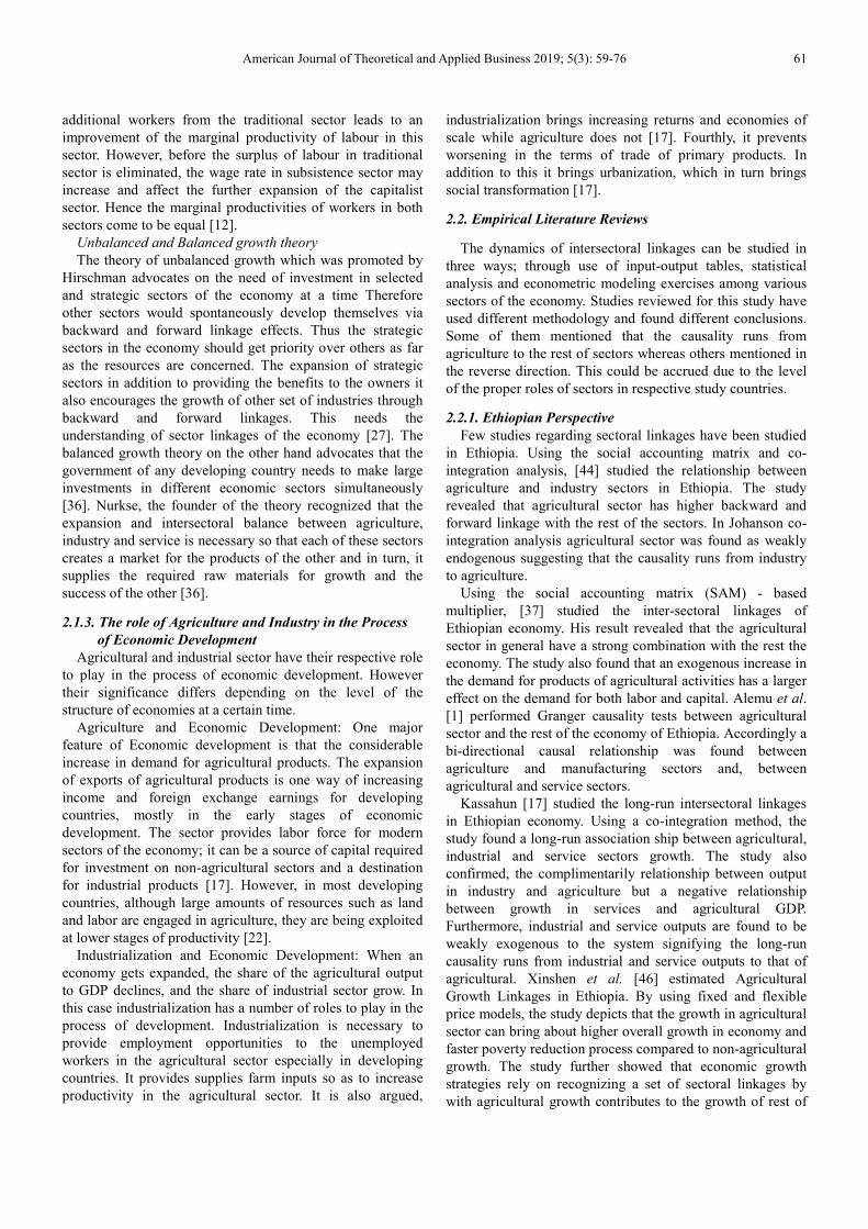
Source: author’s computation based on MoFEC Data.
Figure 1. Sectoral value added shares and economic growth.
‘Figure 1’ depicts the sectoral share of GDP and economic
growth over the study period (the left hand vertical axis
represents the sectoral share to GDP in percentage and the
right side vertical axis shows the GDP in million Birr). The
share of agriculture sector was dominant up to the year 2011.
It was covering more than 45% of the national output.
Starting 2011 year the service sector came to the lead, while
the industry sector is fluctuating between 7 and 14 percent.
The share of agricultural sector has been declining almost
throughout the study year while the share of service sector
has increasing. This is due to the fact that different service
components like: banking and insurance, education and
training centres, health institutions, different transport
services, trade, tellecomunication infrastractures, hotel and
toursim servises are expanding following the eonomc growth
and globalization. The share Agriculture sector especially
starting from the year 1992 onwards has been declining.
However, since the sector is leading in terms of employment
source of inputs and foreign exchange earnings, the declining
share of agriculture in GDP does not mean the role of the
sector is shrinking.
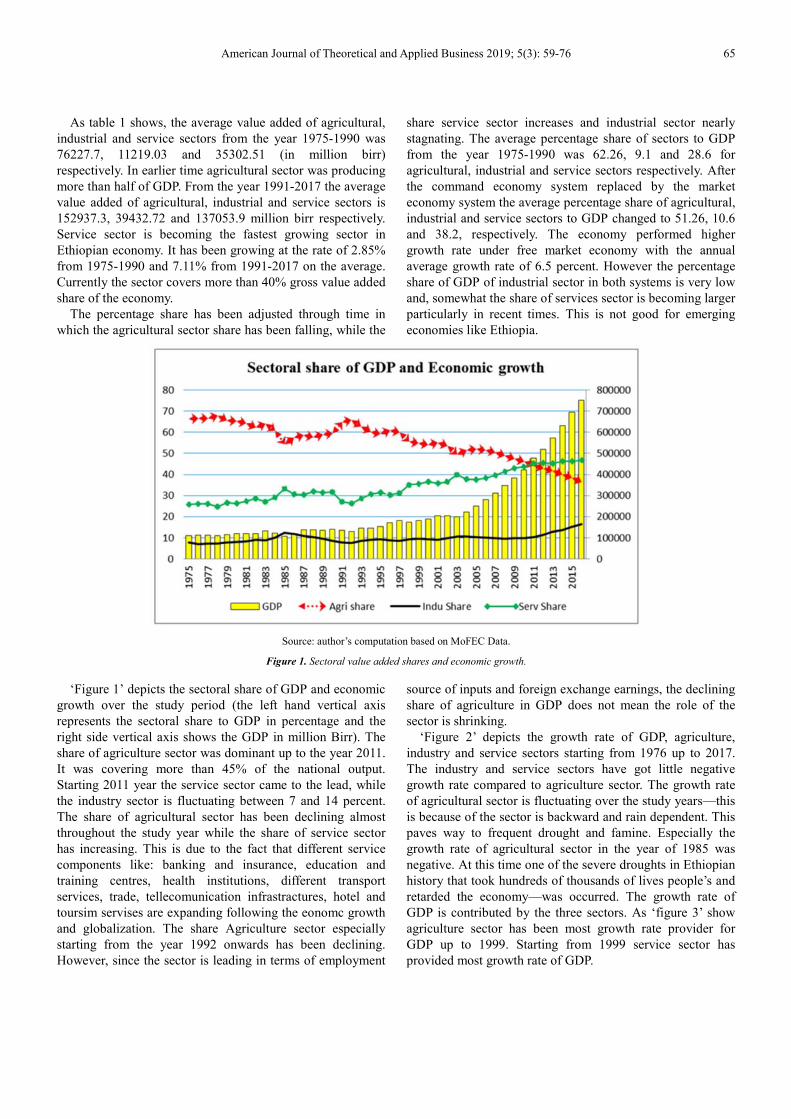
‘Figure 2’ depicts the growth rate of GDP, agriculture,
industry and service sectors starting from 1976 up to 2017.
The industry and service sectors have got little negative
growth rate compared to agriculture sector. The growth rate
of agricultural sector is fluctuating over the study years—this
is because of the sector is backward and rain dependent. This
paves way to frequent drought and famine. Especially the
growth rate of agricultural sector in the year of 1985 was
negative. At this time one of the severe droughts in Ethiopian
history that took hundreds of thousands of lives people’s and
retarded the economy—was occurred. The growth rate of
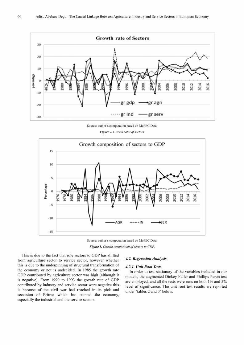
GDP is contributed by the three sectors. As ‘figure 3’ show
agriculture sector has been most growth rate provider for
GDP up to 1999. Starting from 1999 service sector has
provided most growth rate of GDP.
66 Adisu Abebaw Degu: The Causal Linkage Between Agriculture, Industry and Service Sectors in Ethiopian Economy
Source: author’s computation based on MoFEC Data.
Figure 2. Growth rates of sectors.
Source: author’s computation based on MoFEC Data.
Figure 3. Growth composition of sectors to GDP.
This is due to the fact that role sectors to GDP has shifted
from agriculture sector to service sector, however whether
this is due to the underpinning of structural transformation of
the economy or not is undecided. In 1985 the growth rate
GDP contributed by agriculture sector was high (although it
is negative). From 1990 to 1993 the growth rate of GDP
contributed by industry and service sector were negative this
is because of the civil war had reached in its pick and
secession of Eritrea which has stunted the economy,
especially the industrial and the service sectors.
4.2. Regression Analysis
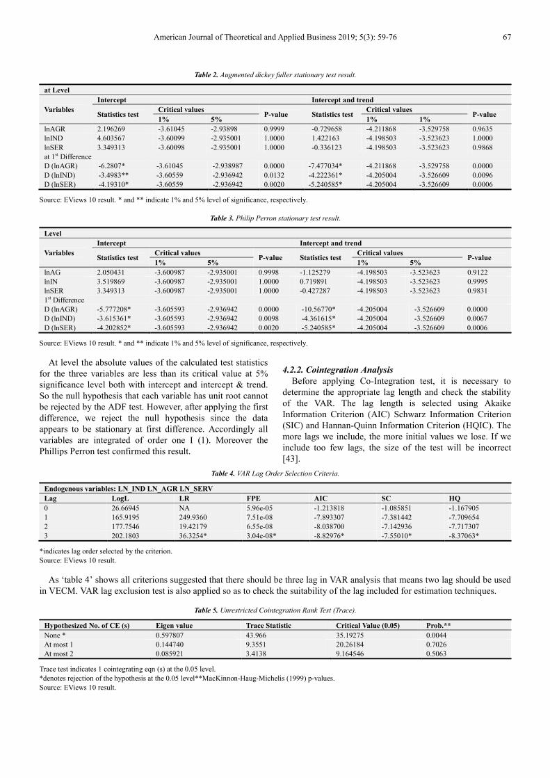
4.2.1. Unit Root Tests
In order to test stationary of the variables included in our
models, the augmented Dickey Fuller and Phillips Peron test
are employed, and all the tests were runs on both 1% and 5%
level of significance. The unit root test results are reported
under ‘tables 2 and 3’ below.
American Journal of Theoretical and Applied Business 2019; 5(3): 59-76 67
Table 2. Augmented dickey fuller stationary test result.
at Level
Variables
Intercept Intercept and trend
Statistics test Critical values
P-value Statistics test Critical values
P-value 1% 5% 1% 1%
lnAGR 2.196269 -3.61045 -2.93898 0.9999 -0.729658 -4.211868 -3.529758 0.9635
lnIND 4.603567 -3.60099 -2.935001 1.0000 1.422163 -4.198503 -3.523623 1.0000
lnSER 3.349313 -3.60098 -2.935001 1.0000 -0.336123 -4.198503 -3.523623 0.9868
at 1st Difference
D (lnAGR) -6.2807* -3.61045 -2.938987 0.0000 -7.477034* -4.211868 -3.529758 0.0000
D (lnIND) -3.4983** -3.60559 -2.936942 0.0132 -4.222361* -4.205004 -3.526609 0.0096
D (lnSER) -4.19310* -3.60559 -2.936942 0.0020 -5.240585* -4.205004 -3.526609 0.0006
Source: EViews 10 result. * and ** indicate 1% and 5% level of significance, respectively.
Table 3. Philip Perron stationary test result.
Level
Variables
Intercept Intercept and trend
Statistics test Critical values
P-value Statistics test Critical values
P-value 1% 5% 1% 5%
lnAG 2.050431 -3.600987 -2.935001 0.9998 -1.125279 -4.198503 -3.523623 0.9122
lnIN 3.519869 -3.600987 -2.935001 1.0000 0.719891 -4.198503 -3.523623 0.9995
lnSER 3.349313 -3.600987 -2.935001 1.0000 -0.427287 -4.198503 -3.523623 0.9831
1st Difference
D (lnAGR) -5.777208* -3.605593 -2.936942 0.0000 -10.56770* -4.205004 -3.526609 0.0000
D (lnIND) -3.615361* -3.605593 -2.936942 0.0098 -4.361615* -4.205004 -3.526609 0.0067
D (lnSER) -4.202852* -3.605593 -2.936942 0.0020 -5.240585* -4.205004 -3.526609 0.0006
Source: EViews 10 result. * and ** indicate 1% and 5% level of significance, respectively.
At level the absolute values of the calculated test statistics
for the three variables are less than its critical value at 5%
significance level both with intercept and intercept & trend.
So the null hypothesis that each variable has unit root cannot
be rejected by the ADF test. However, after applying the first
difference, we reject the null hypothesis since the data
appears to be stationary at first difference. Accordingly all
variables are integrated of order one I (1). Moreover the
Phillips Perron test confirmed this result.
4.2.2. Cointegration Analysis
Before applying Co-Integration test, it is necessary to
determine the appropriate lag length and check the stability
of the VAR. The lag length is selected using Akaike
Information Criterion (AIC) Schwarz Information Criterion
(SIC) and Hannan-Quinn Information Criterion (HQIC). The
more lags we include, the more initial values we lose. If we
include too few lags, the size of the test will be incorrect
[43].
Table 4. VAR Lag Order Selection Criteria.
Endogenous variables: LN_IND LN_AGR LN_SERV
Lag LogL LR FPE AIC SC HQ
0 26.66945 NA 5.96e-05 -1.213818 -1.085851 -1.167905
1 165.9195 249.9360 7.51e-08 -7.893307 -7.381442 -7.709654
2 177.7546 19.42179 6.55e-08 -8.038700 -7.142936 -7.717307
3 202.1803 36.3254* 3.04e-08* -8.82976* -7.55010* -8.37063*
*indicates lag order selected by the criterion.
Source: EViews 10 result.
As ‘table 4’ shows all criterions suggested that there should be three lag in VAR analysis that means two lag should be used
in VECM. VAR lag exclusion test is also applied so as to check the suitability of the lag included for estimation techniques.
Table 5. Unrestricted Cointegration Rank Test (Trace).
Hypothesized No. of CE (s) Eigen value Trace Statistic Critical Value (0.05) Prob.**
None * 0.597807 43.966 35.19275 0.0044
At most 1 0.144740 9.3551 20.26184 0.7026
At most 2 0.085921 3.4138 9.164546 0.5063
Trace test indicates 1 cointegrating eqn (s) at the 0.05 level.
*denotes rejection of the hypothesis at the 0.05 level**MacKinnon-Haug-Michelis (1999) p-values.
Source: EViews 10 result.
68 Adisu Abebaw Degu: The Causal Linkage Between Agriculture, Industry and Service Sectors in Ethiopian Economy
Since regime change (policy variation) and drought highly
affect the number of co-integration among the sectors, the
study treated these variables as an exogenous—by assigning
dummies. Accordingly, ‘0’ is assigned for command
economy (prior to 1991) and ‘1’ for Market economy
(EPDRF era). Similarly ‘0’ and ‘1’ is assigned for the year
that with and without extreme drought, respectively.
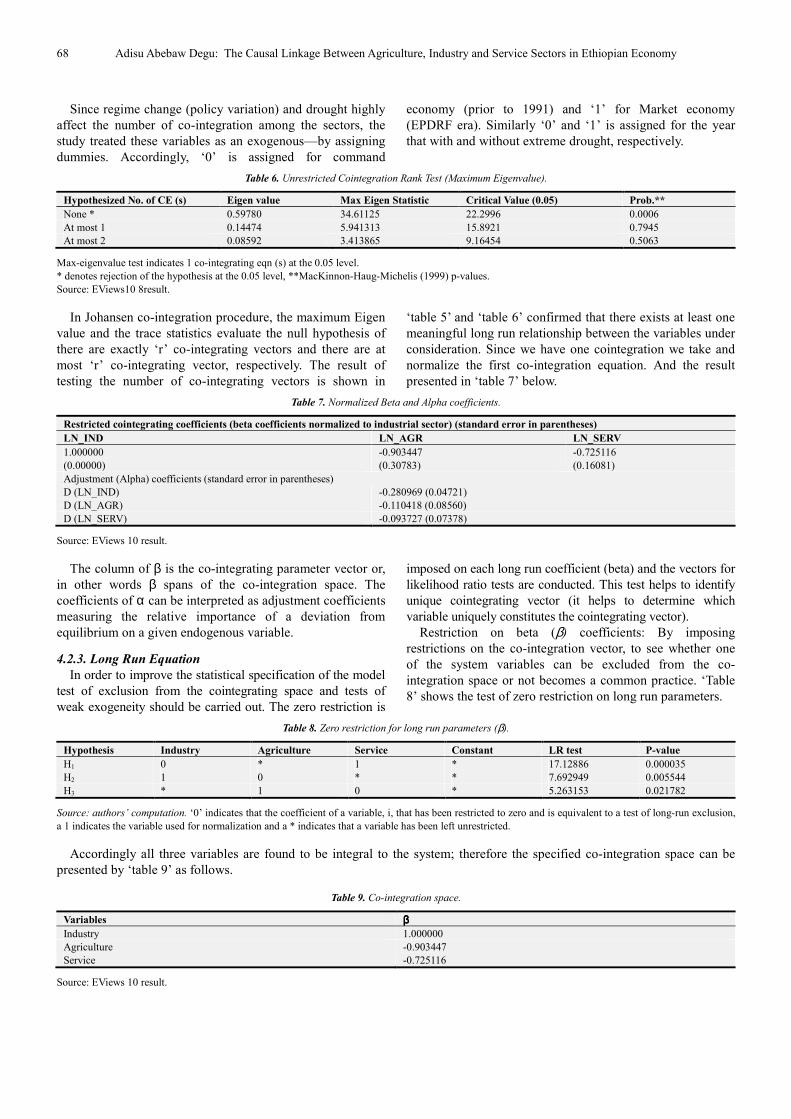
Table 6. Unrestricted Cointegration Rank Test (Maximum Eigenvalue).
Hypothesized No. of CE (s) Eigen value Max Eigen Statistic Critical Value (0.05) Prob.**
None * 0.59780 34.61125 22.2996 0.0006
At most 1 0.14474 5.941313 15.8921 0.7945
At most 2 0.08592 3.413865 9.16454 0.5063
Max-eigenvalue test indicates 1 co-integrating eqn (s) at the 0.05 level.
* denotes rejection of the hypothesis at the 0.05 level, **MacKinnon-Haug-Michelis (1999) p-values.
Source: EViews10 8result.
In Johansen co-integration procedure, the maximum Eigen
value and the trace statistics evaluate the null hypothesis of
there are exactly ‘r’ co-integrating vectors and there are at
most ‘r’ co-integrating vector, respectively. The result of
testing the number of co-integrating vectors is shown in
‘table 5’ and ‘table 6’ confirmed that there exists at least one
meaningful long run relationship between the variables under
consideration. Since we have one cointegration we take and
normalize the first co-integration equation. And the result
presented in ‘table 7’ below.
Table 7. Normalized Beta and Alpha coefficients.
Restricted cointegrating coefficients (beta coefficients normalized to industrial sector) (standard error in parentheses)
LN_IND LN_AGR LN_SERV
1.000000 -0.903447 -0.725116
(0.00000) (0.30783) (0.16081)
Adjustment (Alpha) coefficients (standard error in parentheses)
D (LN_IND) -0.280969 (0.04721)
D (LN_AGR) -0.110418 (0.08560)
D (LN_SERV) -0.093727 (0.07378)
Source: EViews 10 result.
The column of β is the co-integrating parameter vector or,
in other words β spans of the co-integration space. The
coefficients of α can be interpreted as adjustment coefficients
measuring the relative importance of a deviation from
equilibrium on a given endogenous variable.
4.2.3. Long Run Equation
In order to improve the statistical specification of the model
test of exclusion from the cointegrating space and tests of
weak exogeneity should be carried out. The zero restriction is
imposed on each long run coefficient (beta) and the vectors for
likelihood ratio tests are conducted. This test helps to identify
unique cointegrating vector (it helps to determine which
variable uniquely constitutes the cointegrating vector).
Restriction on beta (β) coefficients: By imposing
restrictions on the co-integration vector, to see whether one
of the system variables can be excluded from the co-
integration space or not becomes a common practice. ‘Table
8’ shows the test of zero restriction on long run parameters.
Table 8. Zero restriction for long run parameters (β).
Hypothesis Industry Agriculture Service Constant LR test P-value
H1 0 * 1 * 17.12886 0.000035
H2 1 0 * * 7.692949 0.005544
H3 * 1 0 * 5.263153 0.021782
Source: authors’ computation. ‘0’ indicates that the coefficient of a variable, i, that has been restricted to zero and is equivalent to a test of long-run exclusion,
a 1 indicates the variable used for normalization and a * indicates that a variable has been left unrestricted.
Accordingly all three variables are found to be integral to the system; therefore the specified co-integration space can be
presented by ‘table 9’ as follows.
Table 9. Co-integration space.
Variables ββββ
Industry 1.000000
Agriculture -0.903447
Service -0.725116
Source: EViews 10 result.
American Journal of Theoretical and Applied Business 2019; 5(3): 59-76 69
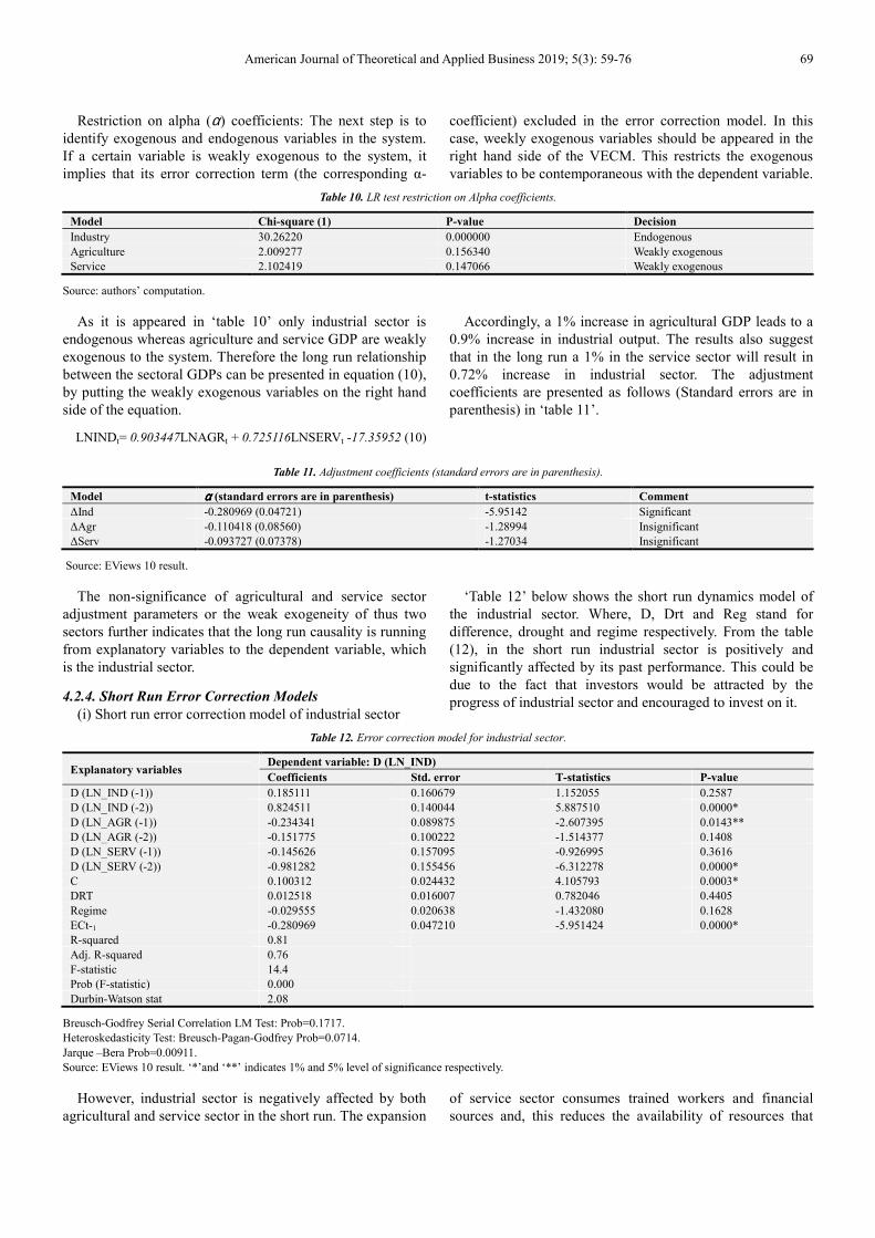
Restriction on alpha (α) coefficients: The next step is to
identify exogenous and endogenous variables in the system.
If a certain variable is weakly exogenous to the system, it
implies that its error correction term (the corresponding α-
coefficient) excluded in the error correction model. In this
case, weekly exogenous variables should be appeared in the
right hand side of the VECM. This restricts the exogenous
variables to be contemporaneous with the dependent variable.
Table 10. LR test restriction on Alpha coefficients.
Model Chi-square (1) P-value Decision
Industry 30.26220 0.000000 Endogenous
Agriculture 2.009277 0.156340 Weakly exogenous
Service 2.102419 0.147066 Weakly exogenous
Source: authors’ computation.
As it is appeared in ‘table 10’ only industrial sector is
endogenous whereas agriculture and service GDP are weakly
exogenous to the system. Therefore the long run relationship
between the sectoral GDPs can be presented in equation (10),
by putting the weakly exogenous variables on the right hand
side of the equation.
LNINDt= 0.903447LNAGRt + 0.725116LNSERVt -17.35952 (10)
Accordingly, a 1% increase in agricultural GDP leads to a
0.9% increase in industrial output. The results also suggest
that in the long run a 1% in the service sector will result in
0.72% increase in industrial sector. The adjustment
coefficients are presented as follows (Standard errors are in
parenthesis) in ‘table 11’.
Table 11. Adjustment coefficients (standard errors are in parenthesis).
Model αααα (standard errors are in parenthesis) t-statistics Comment
∆Ind -0.280969 (0.04721) -5.95142 Significant
∆Agr -0.110418 (0.08560) -1.28994 Insignificant
∆Serv -0.093727 (0.07378) -1.27034 Insignificant
Source: EViews 10 result.
The non-significance of agricultural and service sector
adjustment parameters or the weak exogeneity of thus two
sectors further indicates that the long run causality is running
from explanatory variables to the dependent variable, which
is the industrial sector.
4.2.4. Short Run Error Correction Models
(i) Short run error correction model of industrial sector
‘Table 12’ below shows the short run dynamics model of
the industrial sector. Where, D, Drt and Reg stand for
difference, drought and regime respectively. From the table
(12), in the short run industrial sector is positively and
significantly affected by its past performance. This could be
due to the fact that investors would be attracted by the
progress of industrial sector and encouraged to invest on it.
Table 12. Error correction model for industrial sector.
Explanatory variables Dependent variable: D (LN_IND)
Coefficients Std. error T-statistics P-value
D (LN_IND (-1)) 0.185111 0.160679 1.152055 0.2587
D (LN_IND (-2)) 0.824511 0.140044 5.887510 0.0000*
D (LN_AGR (-1)) -0.234341 0.089875 -2.607395 0.0143**
D (LN_AGR (-2)) -0.151775 0.100222 -1.514377 0.1408
D (LN_SERV (-1)) -0.145626 0.157095 -0.926995 0.3616
D (LN_SERV (-2)) -0.981282 0.155456 -6.312278 0.0000*
C 0.100312 0.024432 4.105793 0.0003*
DRT 0.012518 0.016007 0.782046 0.4405
Regime -0.029555 0.020638 -1.432080 0.1628
ECt-1 -0.280969 0.047210 -5.951424 0.0000*
R-squared 0.81
Adj. R-squared 0.76
F-statistic 14.4
Prob (F-statistic) 0.000
Durbin-Watson stat 2.08
Breusch-Godfrey Serial Correlation LM Test: Prob=0.1717.
Heteroskedasticity Test: Breusch-Pagan-Godfrey Prob=0.0714.
Jarque –Bera Prob=0.00911.
Source: EViews 10 result. ‘*’and ‘**’ indicates 1% and 5% level of significance respectively.
However, industrial sector is negatively affected by both
agricultural and service sector in the short run. The expansion
of service sector consumes trained workers and financial
sources and, this reduces the availability of resources that
70 Adisu Abebaw Degu: The Causal Linkage Between Agriculture, Industry and Service Sectors in Ethiopian Economy
could have been used by industrial sector. The growth of
agriculture sector also possibly will result in increases
consumption of productive resources, which is being used by
industrial sector. The coefficient of the ECt-1 has negative
sign and it is significant for the industry sector approving
further that the variables in the system have a long-run
association ship. The estimated coefficient of ECt-1 is -0.28
which implies that about 28% of the short-run deviations
from industry sector will be adjusted each year to the long-
run equilibrium level of industry sector. However, the
coefficients of drought and regime are insignificant implying
that in the short run they are inconsequential concerning the
performance industrial sector.
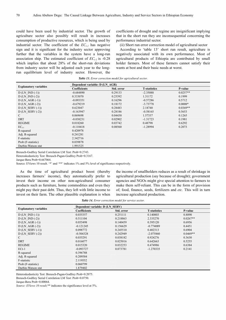
(ii) Short run error correction model of agricultural sector
According to ‘table 13’ short run result, agriculture is
negatively associated with its own performance. Most of
agricultural products of Ethiopia are contributed by small
holder farmers. Most of these farmers cannot satisfy their
wants at best and their basic needs at worst.
Table 13. Error correction model for agricultural sector.
Explanatory variables Dependent variable: D (LN_AGR)
Coefficients Std. error T-statistics P-value
D (LN_IND (-1)) -0.684890 0.29133 -2.35088 0.0257**
D (LN_IND (-2)) 0.333070 0.25392 1.31172 0.1999
D (LN_AGR (-1)) -0.093351 0.16296 -0.57286 0.5712
D (LN_AGR (-2)) -0.679219 0.18172 -3.73778 0.0008*
D (LN_SERV (-1)) 0.623047 0.28483 2.18740 0.0369**
D (LN_SERV (-2)) -0.163947 0.28186 -0.58165 0.5653
C 0.069698 0.04430 1.57337 0.1265
DRT -0.038231 0.02902 -1.31723 0.1981
REGIME 0.018260 0.03742 0.48798 0.6292
ECt-1 -0.110418 0.08560 -1.28994 0.2073
R-squared 0.420978
Adj. R-squared 0.241281
F-statistic 2.342716
Prob (F-statistic) 0.039878
Durbin-Watson stat 1.991525
Breusch-Godfrey Serial Correlation LM Test: Prob=0.2743.
Heteroskedasticity Test: Breusch-Pagan-Godfrey Prob=0.3167.
Jarque-Bera Prob=0.667064.
Source: EViews 10 result. ‘*’ and ‘**’ indicates 1% and 5% level of significance respectively.
As the time of agricultural product boost (thereby
increases farmers’ income), they automatically prefer to
invest their income on other non-agricultural consumer
products such as furniture, home commodities and even they
might pay their past debt. Thus, they left with little income to
invest on their farm. The other plausible explanation is when
the income of smallholders reduces as a result of shrinkage in
agricultural production (say because of drought); government
agencies and NGOs might give special attention to farmers to
make them self-reliant. This can be in the form of provision
of; food, finance, seeds, fertilizers and etc. This will in turn
increase agricultural production.
Table 14. Error correction model for service sector.
Explanatory variables Dependent variable: D (LN_SERV)
Coefficients Std. error T-statistics P-value
D (LN_IND (-1)) 0.035357 0.251111 0.140803 0.8890
D (LN_IND (-2)) 0.511104 0.218863 2.335270 0.0267**
D (LN_AGR (-1)) 0.055498 0.140459 0.395120 0.6956
D (LN_AGR (-2)) -0.121245 0.156629 -0.774089 0.4451
D (LN_SERV (-1)) 0.098772 0.245510 0.402313 0.6904
D (LN_SERV (-2)) -0.504328 0.242949 -2.075860 0.0469**
C 0.035291 0.038182 0.924276 0.3630
DRT 0.016077 0.025016 0.642663 0.5255
REGIME 0.015320 0.032253 0.474986 0.6384
ECt-1 -0.093727 0.073781 -1.270335 0.2141
R-squared 0.396788
Adj. R-squared 0.209584
F-statistic 2.119552
Prob (F-statistic) 0.060799
Durbin-Watson stat 1.879402
Heteroskedasticity Test: Breusch-Pagan-Godfrey Prob=0.2075.
Breusch-Godfrey Serial Correlation LM Test: Prob=0.0750.
Jarque-Bera Prob=0.00064.
Source: EViews 10 result,** indicates the significance level at 5%.

American Journal of Theoretical and Applied Business 2019; 5(3): 59-76 71
Agricultural sector also negatively affected by one year
earlier performance of industrial sector, and positively lagged
service and industrial output. Drought, although statistically
insignificant, affects agricultural sector negatively—as it was
expected. The EPDRF regime influences agricultural sector
positively but not statistically significant. The error
correction term, however, is not significant.
(iii) Short run error correction model of service sector
As depicted by ‘table 14’ above, service sector is positively
and significantly affected by lagged value of industrial sector.
This means that industrial sector can provide different products
such as; alcohol & beverage, solar pulbs, cell phones etc. for
sale. The expansion of telecommunication, road infrastructure
and maintenance services could be as a result of boost in
building & construction, technology, metal & iron production -
through backward and forward linkage. The growth of industrial
production expands domestic markets which further arouse
trading and commercial activities.
Agricultural sector affects the sector positively in first lag
and negatively second lag although both are insignificant.
Drought has a positive effect on service sector in the short-run.
The vast population in Ethiopia lives in rural areas under
which agricultural and related activities are dominant. In
addition agricultural sector is a rain dependent which is always
uncertain. This is because of the inconsistence of rainfall and
climate condition of the country. At the time of rain failure,
such large populations expose to drought and strive and begin
migrating to urban areas. Therefore, due to the shrink in
agricultural sector, some resources; such as labour force, shifts
to service sector (such as urban informal sector). The
occurrence of drought also diverts the government to focus on
activities that are related to health care and nutrition. Regime
also has a positive but insignificant effect on the service sector
growth. Dergue regime gave less attention to private
enterprises, private companies and other business
organizations such as banks, insurances, exports and importers.
Model diagnostic tests
The three common criterions for model specification are: the
residual of the model should be normally, Heteroskedasticity
and serial correlation. First, the residuals are tested for normal
distribution for each three models. The results of the test show
that the residuals of both industrial and service sector models
are not normally distributed. However, some researchers [2,
30] argue that the model can be accepted even though the
residuals are not normally distributed. Second, the null-
hypothesis of there is no Heteroskedasticity is tested and the
results of the three models show that the value of test statistics
(Obs*R2) is greater than 0.05 implying, the H0: the residuals
are homoscedastic is accepted. Third, the test conducted for
serial correlation (Breusch-Godfrey Serial Correlation LM
Test) is tested for all models and the probability value of
Obs*R2
is greater than 0.05 for all models implying the
residuals are not serially correlated. In addition to this,
CUSUM test conducted. The null hypothesis of this test is that
there is no structural break. Accordingly the Dummy variable
is found enough to reflect the structural breaks over the study
period. The results of CUSUM tests for industrial, agricultural
and service sectors are reported in ‘Figure 4’, ‘Figure 5’ and
‘Figure 6’, respectively.
Figure 4. CUSUM test for industry sector.
Figure 5. CUSUM test for Agriculture sector.
Source: EViews 10 result.
Figure 6. CUSUM test for service sector.

72 Adisu Abebaw Degu: The Causal Linkage Between Agriculture, Industry and Service Sectors in Ethiopian Economy
4.2.5. Causality Analysis
(i) Short run causality
The short-run causality can be determined using a test on
the joint significance of the lagged independent variables,
using an F-test or Wald test. The null hypothesis is the lagged
values of the independent variable are jointly Zero, meaning
there is no short run causality running from the independent
variables to the dependent one. The short run causality test
result is presented in ‘table 15’. From short-run causality
analysis there is bi-directional causality between; industrial
and service sectors, industrial and agricultural sectors and
uni-directional causality between service sector and
agricultural sector running from service to agricultural sector.
But there is no causality between service sector and
agricultural sectors running from agricultural to service
sector.
Table 15. VEC Granger Causality/Block Exogeneity Wald Tests.
VEC Granger Causality/Block Exogeneity Wald Tests
Sample: 1975 2017
Dependent variable: D (LN_IND)
Excluded Chi-sq df Prob. Conclusion
D (LN_AGR) 7.74494 2 0.0208** Agriculture sector granger causes Industry sector
D (LN_SERV) 42.9324 2 0.0000* Service sector granger causes Industry sector
Dependent variable: D (LN_AGR)
Excluded Chi-sq df Prob.
D (LN_IND) 5.68155 2 0.0584*** Industry sector granger cause agriculture sector
D (LN_SERV) 4.87567 2 0.0873*** service sector granger cause agriculture sector
Dependent variable: D (LN_SERV)
Excluded Chi-sq df Prob.
D (LN_IND) 6.86498 2 0.0323** Industry sector granger causes service sector
D (LN_AGR) 0.93147 2 0.6277 Agriculture does not granger cause service sector
Source: EViews 10 result. *, **and *** indicates a 1%, 5% and 10% level of significance respectively.
(ii) Long run Causality
From the vector error correction models, although all error
correction terms are negative and less than one, only the
industry sector equation is significant, implying the long-run
causality is running from Agricultural and Service sector to
the industry sector. Our long-run causality showed that, there
is uni-directional causality between agricultural and
industrial sectors running from agricultural sector to
industrial sector, and between industrial and service sectors
running from service sector to industrial sector. The absence
of any long run causality between agricultural and service
sectors reveals the weak long run association between them.
The recent expansion of service sector at least is not preceded
by the performance of agricultural sector. As part of service
sector is determined by globalization and not merely depends
on the performance of domestic economy, the neutrality of
this sector with agriculture may not be a surprise result. The
absence of long run causality between agricultural and
service sectors also proves in the long run the performance of
agricultural sector is not depending on service sector.
4.2.6. Variance Decomposition
The magnitude of variance explained is determined to be
at the 10th
time horizon for all sectors and the result is
presented in ‘table 16’.
Table 16. Magnitude of Variance explained at the 10th Time Horizon by
Different Components.
At 10th Time Horizon S. E Percent
Variance in Industry explained by Agriculture 0.263775 47.80998
Variance in Industry explained by Service 0.263775 24.75254
Variance in Industry explained by itself 0.263775 27.43748
Variance in Agriculture explained by Industry 0.217173 9.934834
Variance in Agriculture explained by Service 0.217173 13.26301
At 10th Time Horizon S. E Percent
Variance in Agriculture explained by itself 0.217173 76.80216
Variance in Service explained by Industry 0.267183 41.09870
Variance in Service explained by Agriculture 0.267183 21.31639
Variance in Service explained by itself 0.267183 37.58491
Source: author’s computation.
Variance Decomposition of industrial sector: From the
‘table 16’ we can observe that agriculture sector alone
explained 47.8 percent variance in industry sector at the
10th
time horizon, whereas the service sector explains 24.7
percent variance of industry sector. The remaining 27.43
percent of variance is explained by industry sector itself.
Hence, the industry sector is strongly affected by agriculture
sector in the long run, and, thus the long run causality seems
to run from agriculture sector to industrial sector.
Furthermore, starting from 5th
time horizon agriculture sector
starts to explain much of variance in industrial sector. From
the above justification, we can understand that in the long run
agriculture sector can be the springboard to industrial sector.
Variance Decomposition of agricultural sector: Likewise, it
is observed that 9.9 percent variance in agriculture is
explained by industry sector, while service sector explains
13.26 percent variance in agriculture sector at the 10th
year
time horizon. Here 76.8 percent of variance on agriculture
comes out from itself. This shows that in the long run both
service and industry sectors cause the agriculture sector less.
Variance decomposition of service sector: From the service
sector it is observed that about 41 percent variance in service
explained at the 10th time horizon is explained by Industry
sector, whereas agriculture explains 21.3 percent variance in
service sector at the same time horizon and the remaining
21.3 percent is explained by service sector itself. Hence, the
industry sector affects service sector strongly in the long-run,

American Journal of Theoretical and Applied Business 2019; 5(3): 59-76 73
and, the causality seems to run from industry sector to
service sector. Industry sector can support service sector
through providing different produced items.
4.2.7. Impulse Response
From impulse response results reported under ‘figure 7’
we can observe that agricultural sector highly affects the
growth of industrial sector positively, after three periods of
innovation. For service sector however, it has a negative
effect up to 5 year and a positive effect after 5 year of
innovation. The industrial sector as has a positive impact on
service sector while, it has a small positive impact on
agricultural sector after an innovation. The service sector has
a negative impact on industrial sector up to five year, but has
a big positive impact afterwards. The service sector also has
appositive but a declining impact on agricultural sector.
Therefore, the results of both IRs and VDs methods suggest
that the agricultural sector can be playing the main role in
influencing the overall growth of the economy via its
linkages to other sector. This result can also be confirmed
from our long run results.
Figure 7. Impulse response functions.
Source: EViews 10 result.
Note: Y axis measures the impact and the X axis denotes the time trend.
5. Conclusion and Recommendation
5.1. Conclusion
The study analyzed intersectoral linkages in Ethiopian
economy using a time series value added data on industrial,
agricultural and service sectors ranging from 1975 to 2017.
The study employed Johanson cointegration test, vector error
correction (VECM) or restricted vector autoregressive (VAR)
model granger causality test, variance decomposition
functions and impulse response. The study found a stable
long run relationship among three major sectors of the
economy. Only the industrial sector is found to be
endogenous to the system. The result is inconsistent with a
similar study conducted by [17], whose study found that only
agricultural sector is endogenous to the system.
The exogeneity of agricultural and service sectors indicate
that, the causality is running from these two sectors to
industrial sector. Here, it is agricultural and service sector
that causes industrial sector. This result is not a surprise in a
developing country whose economy is mainly dominated by
agricultural sector, and where the service sector grows

74 Adisu Abebaw Degu: The Causal Linkage Between Agriculture, Industry and Service Sectors in Ethiopian Economy
dramatically before conventional structural transformation
transpired, through industrialization. The absence long run
causality between agricultural and service sectors reveals the
weak long run association between these sectors. In other
words the recent expansion of service sector at least is not
caused by the performance of agricultural sector. In the same
fashion, in the long run the performance of agricultural sector
is not depending on service sector. In the short run there is
bi-directional causality between industrial and agricultural
sector, and between industrial and service sector. The study
also found that there exist uni-directional causality between
service and agricultural sectors running from service to
agricultural sector. However the result of long run causality
is inconsistent with the short run one.
From dynamic causality analysis of variance
decomposition, agricultural sector explained 47.8 percent
variance in industry sector at the 10th
time horizon, thus
industrial sector is strongly affected by agriculture sector,
and the long run causality runs from agriculture sector to
industrial sector. 41 percent variance in service sector
explained at the 10th
time horizon is explained by Industrial
sector, thus causality looks to run from industry sector to
service sector. However, the predominance of service sector
over industrial sector in under developed economy is not
preferable, at least at early stage of development. Hence, the
results of both Impulse response and Variance decomposition
identify that agricultural sector as the major economic
activity that controls and affects most of economic activities
in Ethiopia. The sector has a dynamic effect on industrial
sector. From our descriptive analysis part the share of
agricultural sector has been declining significantly over the
study period. The sector covered 66% of GDP in 1975 which
has declined to 36% in 2017. Moreover most of the variation
in growth rate of GDP comes from agricultural sector. This
shows that how the economy depends on agricultural sector.
Therefore, the declining percentage share of agricultural
sector to GDP doesn’t exhibit the true structural
transformation. The analysis of intersectoral linkages
identified agricultural sector as the core economic activity
that controls most economic activities in Ethiopia.
5.2. Recommendations
From the study result we have found that agricultural and
service sectors are exogenous and industrial sector as
endogenous to the system. Hence as long as industrialization is
a big concern of sustainable and lasting development, policies
that increase the linkage between agricultural and industrial
sectors are preferable. In this regard structural polices like
ADLI, if correctly implemented, will have not only a
transformational upshot but also a sustainable growth effect, as
agricultural sector affects the industry through its causality
linkage. The existence of uni-directional causality between
agricultural and industrial sector in Ethiopia provides a support
for the need of increasing resources to agricultural research,
rural and infrastructural development. A developing country
like Ethiopia which is food insecure, its economic growth
could be driven by policies that promote agriculture. The weak
linkage between agricultural and service sectors can be related
directly to the problems of fragile power supply, inadequate
infrastructure, poor marketing chain, low road network,
logistic and etc. The nature of such weak intersectoral
relationships possibly indicates that at least any policy priority
supporting services sector need not necessarily go against
agricultural sector since the services sector causes agricultural
sector at least in the short run.
From standard point of view, in the initial stages of
economic development, most of the economic resources are
allocated to the agricultural sector; but as the economy
progresses, resources are reallocated from agriculture to
industrial and service sectors; as the economy develops
further, resources are again transferred from both agricultural
and industrial sectors to service sector. Hence
industrialization should come after agricultural
transformation achieved. Therefore, the government of
Ethiopia should enhance the agricultural sector through,
mechanization, land defragmentation, irrigation, modern
input supply…etc. that could boost the sector. The declining
agricultural share of GDP doesn’t merely indicate the
existence structural transformation and the sector is still the
pillar of the economy as confirmed by causality analysis.
Moreover, the three sectors are interlinked with each other;
any changes of policy strategy in one sector will
automatically affect the other sectors and the economy in
general. Therefore government or policy makers should
implement policies bearing in mind the linkages and
direction of causality among sectors of the economy.
References
[1] Alemu Z G, K. O. (2003). Contribution of agriculture in the Ethiopian economy: a time-varying parameter approach. Agrekon, 42, 29-48.
[2] Banumathy, K., & Azhagaiah, R. (2015). Long-Run and Short-Run Causality between Stock Price and Gold Price: Evidence of VECM Analysis from India. Management Studies and Economic Systems (MSES), 247-256.
[3] Bathla, S. (2003). Inter-sectoral growth linkages in India: implications for policy and liberalized reforms. India.
[4] Berhanu, N. (1996). Development Options for Ethiopia: Rural, Urban or Balanced.
[5] Chebbi, H. E. (2010). Agriculture and economic growth in Tunisia. China agricultural Economic review, 2 (1), 63-78.
[6] Engle, R., & Granger, C. W. (1987). Co-Integration and Error Correction: Representation, Estimation, and Testing. Econometrica, 55 (2), 251-276.
[7] Erjavec, N., & Cota, B. (2003). Macroeconomic granger-causal dynamics in Croatia: evidence based on a vector error-correction modeling analysis. Ekonomski pregled, 54 (1-2), 139-156.
[8] Fantu, C. (2016). Structural Transformation in Ethiopia: The Urban Dimension. ECPI Discussion Paper Final Stockholm International Peace Research Institute.
American Journal of Theoretical and Applied Business 2019; 5(3): 59-76 75
[9] Fasikaw A. (2018). An Empirical Investigation of Inter Sectoral Linkage in Ethiopia: A Co-Integrated VECM Approach, June, 2018 Addis Ababa university, Ethiopia. Unpublished thesis paper.
[10] Geda, A., Zerfu, D., & Ndung’u, N. (2011). Applied Time-Series Econometrics: A Practical guide for Macroeconomic Researchers with a focus on Africa. Central Bank of Kenya, African Economic Research Consortium and Addis Ababa University.
[11] Gunjeet Kaur, S. B. (2009). An empirical investigation on their inter-sectoral linkages in India. Reserve Bank of India Occasional Papers, 30-72.
[12] Hirota, Y. (2002). Reconsidering of the Lewis Model: Growth in a Dual Economy.
[13] James F Oehmke, A. N. (2016). James F Oehmke, Anwar Naseem, Jock Anderson, Carl Pray, Contemporary African Structural transformation: An Empirical Assessment.
[14] João, G., Gilson, P., & Marta C. N., S. (2014). Agriculture in Portugal: linkages with industry and services.
[15] Johansen, S. (1992). Testing Weak Exogeneity and the Order of Cointegration in UK Money Demand. Journal of Policy Modeling, 313-334.
[16] Johansen. (1988). Statistical analysis of co-integrating vectors. Journal of Economic dynamic and control, 12, 231-255.
[17] Kassahun, T. (2006). Dynamic Sectoral Linkages in the Ethiopian Economy: A preliminary Assessment. Addis Ababa: Ethiopian Economic Association /Ethiopian Economic Policy Research Institute.
[18] Katircioglu, S. (n. d). Co-Integration and Causality between GDP, Agriculture, Industry and Services growth in North Cyprus: Evidence from Time Series Data, 1977-2002. Review of Social, Economic & Business Studies, 7/8, 173-187.
[19] Kaur, G., Bordoloi, S., & Rajesh, R. (2009). An empirical investigation on the inter-sectoral linkages in India. Reserve Bank of India.
[20] Kelikume, D. S. (2011). Empirical analysis of the linkages between the manufacturing and other sectors of the Nigerian economy. 150.
[21] Kohansal, M. T. (2013). Agricultural impact on economic growth in Iran using ARDL approach to co-integration. International Journal of Agriculture and Crop Sciences, 1223-1226.
[22] Kym, A. (1987). On Why Agriculture Declines with Economic Growth.
[23] Matahir, H. (2012). The empirical investigation of the nexus between agricultural and industrial sector in Malaysia. International Journal of Business and Social Science, 225-231.
[24] MoFED. (2010). Growth and Transformation Plan (GTP I) 2010/11-2014/15. Addis Ababa: Ministry of Finance and Economic Development.
[25] Naval, M. R. (2016). An Empirical study of Inter-Sectoral Linkages and Economic growth in India. American Journal of Rural Development, 4, 78-84.
[26] NPC. (2016). Growth and Transformation Plan II (2015/16-2019/20). Addis Ababa: National Planning Commission.
[27] Perez, K. K. (2004). Unbalanced growth. National bureau of economic research. NBER working paper series.
[28] Phillips, P. a. (1988). Testing for a Unit root in time series regression. Biometrika,, 335-346.
[29] Rahel, K. (2003). Ethiopia’s recent growth performance: a Survey of the literature.
[30] Roman, T. (2012). The link between financial development and economic growth in Ethiopia. Addis Ababa, Ethiopia: Unpublished thesis paper.
[31] Saikia, D. (2011). Analyzing inter-sectoral linkages in India. African Journal of Agricultural Research, 6 (33), 6766-6775.
[32] Seid, N. (2015). Prospects and Challenges of Structural Transformation in Ethiopia: Assessing the Performance of GTP I and Reflecting on GTP II. Addis Ababa. Ethiopian Economics Association Ethiopian Economic Policy Research Institute.
[33] Sepehrdoust, H., & Adnan, Q. m. (2012). An empirical study of inter-sectoral linkages and Economic growth. Academic Journals Inc., 494-504.
[34] Sikhosana N, T. A. (2015). Inter-sectoral linkages and Agricultural growth in Swaziland for the period 1971-2011. Journal of Economics and Sustainable Development, 6, 218-228.
[35] Subramaniam, V. (2010). Agricultural intersectoral linkages and their contribution to economic development.
[36] Sylvester, A. A., Benedict, U. A., & Effifiom, E. C. (2016). Analysis of the Sectoral Linkages and Growth Prospects in the Nigerian Economy. IOSR Journal of Economics and Finance (IOSR-JEF), 7 (6), 73-80.
[37] Tadele, F. (2000, April). Measuring sectoral interdependence in Ethiopia: a social accounting matrix (SAM) approach. Ethiopian Journal of Economics, IX.
[38] Tadele, F. (2015). Sectoral economic growth and structural transformation in Ethiopia. Department of Economics, Addis Ababa University.
[39] Timmer p., M. M. (2012). Patterns of growth and structural transformation in Africa: trends and lessons for future development strategy. International Food Policy Research Institute.
[40] Uddin, M. M. (2015). Causal Relationship between Agriculture, Industry and Services Sector for GDP Growth in Bangladesh: An Econometric Investigation. Journal of Poverty, Investment and Development, 18, 124-130.
[41] UN-Habitat. (n. d). Structural transformation in developing countries: Cross regional analysis. Nairobi, Kenya.: Structural transformation in developing co United Nations Human Settlements Programme (UN-Habitat).
[42] Verner, N. M. (2001). Inter-sectoral dynamics and economic growth in Ecuador. The World Bank Latin America and the Caribbean Region Economic Policy Sector Unit.
[43] Wooldridge, M. (2000). Introductory Econometrics: A Modern Approach (2 ed.).
[44] Worku Gebeyehu, G. A. (2013). Which Sector Should Lead In Ethiopia? Industry or Agriculture? Addis Ababa: Ethiopian Economic Association.

76 Adisu Abebaw Degu: The Causal Linkage Between Agriculture, Industry and Service Sectors in Ethiopian Economy
[45] Wubshet, O. (2008). The determinant of aggregate import demand in Ethiopia: co integration analysis. Addis Ababa, Ethiopia. unpublished thesis.
[46] Xinshen, D. & Steven Haggblade, B. F. (2007). Agricultural Growth Linkages in Ethiopia: Estimates using Fixed and Flexible Price Models. Washington: international food policy.
[47] https://tradingeconomics.com/ethiopia/gdp-growth-annual 2018.
[48] USAID/Ethiopia Agriculture Knowledge, Learning, Documentation and Policy Project.
Top Related