


Languages
Pages
Legal


Text Messages as MobilizationTools: The Conditional Effect of
Habitual Voting and Election SalienceThe Harvard community has made this
article openly available. Please share howthis access benefits you. Your story matters
Citation Malhotra, Neil, Melissa R. Michelson, Todd Rogers, and Ali AdamValenzuela. "Text Messages as Mobilization Tools: The ConditionalEffect of Habitual Voting and Election Salience." American PoliticsResearch 39.4 (July 2011): 664-681.
Published Version http:dx.doi.org/10.1177/1532673X11398438
Citable link http://nrs.harvard.edu/urn-3:HUL.InstRepos:10471523
Terms of Use This article was downloaded from Harvard University’s DASHrepository, and is made available under the terms and conditionsapplicable to Open Access Policy Articles, as set forth at http://nrs.harvard.edu/urn-3:HUL.InstRepos:dash.current.terms-of-use#OAP

CITE:
Malhotra, N., Michelson, M. R., Rogers, T., & Valenzuela, A. A. (2011). Text Messages as
Mobilization Tools The Conditional Effect of Text Messages as Mobilization Tools The
Conditional Effect of. American Politics Research, 39(4), 664-681.
Text Messages as Mobilization Tools:
The Conditional Effect of Habitual Voting and Election Salience
Neil Malhotra
University of Pennsylvania
238 Stiteler Hall
Philadelphia, PA 19104
(408) 772-7969
Melissa R. Michelson
Menlo College
Todd Rogers
Analyst Institute
Ali Adam Valenzuela
Stanford University
616 Serra Street
Encina Hall West Room 100
Stanford, CA 94305-6044
(650) 723-1806
(650) 723-1808 fax

ABSTRACT
In their 2009 article published in the American Journal of Political Science, Dale and Strauss
(DS) introduce the Noticeable Reminder Theory (NRT) of voter mobilization, which posits that
mobilization efforts that are highly noticeable and salient to potential voters, even if impersonal,
can be successful. In an innovative experimental design, DS show that text messages
substantially boost turnout by levels comparable to personalized mobilization strategies,
challenging previous field experimental research which argues that social connectedness is the
key to increasing participation. This paper replicates DS’s research design and extends it in two
key ways. First, whereas the treatment in DS’s experiment is a “warm” text message that was
combined with some form of contact, we test NRT more cleanly by examining the effect of
“cold” text messages that are completely devoid of auxiliary interaction. Second, because we
have data on subjects’ recent voting histories, we can test an implication of NRT that habitual
voters should exhibit the largest treatment effects in lower-salience elections, whereas casual
voters should exhibit the largest treatment effects in higher-salience elections. Via these two
extensions, we find support for NRT.

1
In their 2009 article published in the American Journal of Political Science, Dale and
Strauss (DS) introduce the Noticeable Reminder Theory (NRT) of voter mobilization, which
posits that mobilization efforts that are highly noticeable and salient to potential voters, even if
impersonal, can be successful. This is in contrast to Social Occasion Theory (SOT), which
suggests that voting is a social occasion, and therefore explains why personal mobilization
strategies such as in-person contact (Gerber and Green 2000) and volunteer telephone calls
(Nickerson 2006) tend to be effective, while impersonal strategies such as direct mail (Gerber
and Green 2000) and electronic mail (Nickerson 2007) are not. The main crux of DS’s logic is
that the weighing of costs and benefits is generally undertaken by citizens at the time of deciding
whether to register to vote in an election, and that conditional on being registered, a voter simply
needs to be reminded to vote in a salient manner (not personally convinced). Conversely, SOT
contends that social contact is necessary to boost the perceived benefits of voting and
consequently the decision to participate.
The bulk of the field experimental literature on voter mobilization has forwarded the
importance of social connectedness (Green and Gerber 2008), which is challenged by DS. In an
innovative experimental design, DS use text messages to distinguish between NRT and SOT.
Like in-person contact and telephone calls, text messages are noticeable and salient. However,
like direct and electronic mail, they are impersonal. Hence, if text messages significantly and
substantially boost turnout at a level similar to that of personalized mobilization strategies, then
it is the noticeability of the message (and not the personalization of the message) that promotes
turnout. Conversely, if the effect of text messages is similar to the effect of direct and electronic
mail, then SOT is supported.
DS find that the intent-to-treat effect of text messages on turnout is 3 percentage points,

2
similar to the average effect of volunteer phone calls and much higher than impersonal modes of
communication such as direct mail, electronic mail, commercial phone calls, and robotic phone
calls. Thus, DS find strong evidence for NRT. In other words, the reason why e-mails and pieces
of direct mail do little to mobilize voters is not because they are impersonal, but rather because
they are not noticeable.
DS also crucially distinguish between mobilization and reminding. Whereas the existing
field experimental literature on turnout presumes that various modes of contact engage voters in
the political process by increasing the perceived benefits of voting, DS argue that the mechanism
is more about scheduling; campaign contact reminds people who are already generally inclined
to vote that they should be doing so in the near future.1
This note highlights two potential limitations of DS’s research design, which we address
via our replication and extension. First, whereas the treatment in DS’s experiment is a “warm”
text message that was combined with some form of contact prior to the delivery of the text, we
test NRT more cleanly by examining the effect of “cold” text messages that are completely
devoid of auxiliary interaction. Second, because we have data on subjects’ recent voting
histories, we can test an implication of NRT that habitual voters should exhibit the largest
treatment effects in lower- salience elections, whereas casual voters should exhibit the largest
treatment effects in higher-salience elections.
Using “Cold” Text Messages to Eliminate Auxiliary Interaction
DS’s treatment was not solely a text message sent to registered voters. Instead,
participants were recruited through one of two mechanisms. Some citizens were registered in
person by Student Public Interest Research Groups (PIRGs). During this registration process, cell
1 Consistent with this argument, recent research shows that explicitly inducing people to develop a plan to vote
increases the effectiveness of GOTV contact (Nickerson and Rogers 2010).

3
phone numbers were captured. Other citizens opted in to the experiment by registering to vote
via a Working Assets website and specifically provided their cell phone number and permission
for the company to contact them via text message in the future. The registration website was
advertised on Google and was sent out by nonprofit organizations to their membership lists. In
other words, part of the sample consisted of people who had previously been in contact with an
organization and requested that they be text messaged in the future.
DS’s experimental treatment is therefore what we refer to as warm texts, or text messages
combined with some sort of auxiliary contact. In the case of the PIRGs, an individual registered
the voter in person. In the case of Working Assets, people did not receive text messages without
warning, but rather asked an organization with which they had a personal connection (i.e. their
nonprofit via Working Assets) to remind them to vote. In the case of individuals who joined the
experiment via a Google advertisement, even these people opted in by responding to the initial
advertisement and giving explicit permission to be contacted via text message in the future. An
additional concern is that the text messages reminded people not only about the upcoming
election, but also that they made an implicit commitment to vote when they registered with the
organization. Consequently, DS cannot disentangle the effect of a noticeable reminder from
social commitment effects.
Hence, DS’s experiment may be unable to distinguish between the two theories of
political participation described above. Proponents of SOT could respond by saying that the
reason the warm texts were successful is not because of their noticeability, but because they
reminded people of the prior contact (sometimes personal) at the time of registration, as well as
the commitment they made to vote. In our extension, we address this criticism by eliminating all
auxiliary contact from the text message treatment.

4
DS respond to this concern by pointing out that an interaction term between closeness of
the registration date to the election (i.e. closeness to the prior contact) and the treatment was
insignificant. However, this test has two main limitations. First, it assumes that the timing of
auxiliary contact significantly influences its efficacy. Second, it assumes that the relationship
between proximity of registration date and treatment efficacy is linear.
A much simpler and straightforward test of NRT is to use cold texts as the treatment. We
define cold texts as text messages that have absolutely no prior or personal contact associated
with them. In other words, people do not receive texts from an organization that registered them
in person, and do not give permission to receive text messages prior to Election Day. Cold texts
more closely approximate the impersonality of electronic and direct mail, but fulfill DS’s
criterion of being noticeable.
Using Voting Histories to Test for Heterogeneous Effects
One important implication of NRT is that the effect of noticeable reminders jointly
depends on: (1) the salience of the election; and (2) an individual’s voting history. DS’s
argument is similar to that of Arceneaux and Nickerson’s (2009) theory of “contingent
mobilization”a noticeable reminder will only affect an individual’s decision to vote if they are
near their indifference threshold. In lower-salience elections, habitual voters (those who vote in
almost every election) are near their indifference thresholds, whereas casual voters (those who
only vote in major, higher-salience elections or those with spotty voting records) are uninterested
in the contests and therefore well below the threshold. Conversely, in higher-salience elections,
casual voters are near their indifference thresholds while habitual voters are more fully engaged
in the contests and therefore far above the threshold and not susceptible to reminders. We
describe each of these theoretical predictions in more detail below.
5
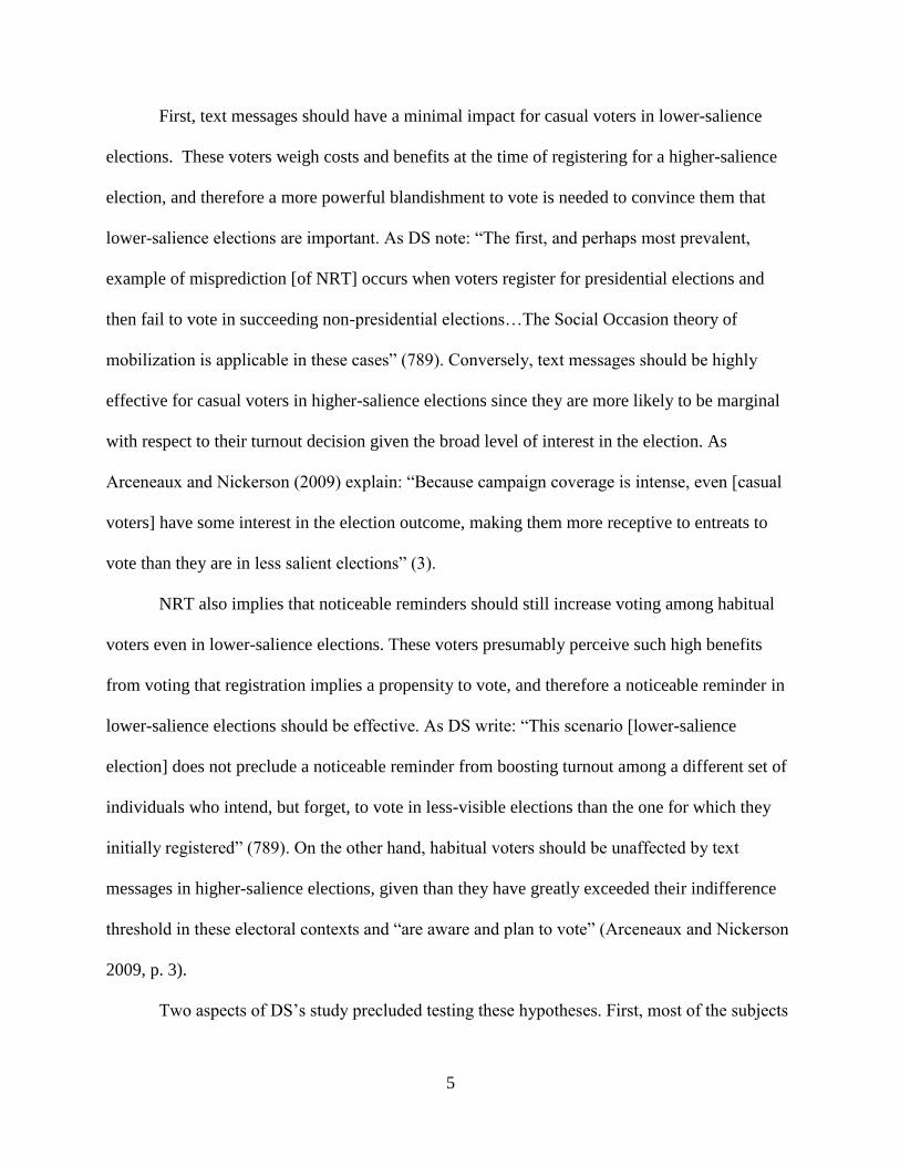
First, text messages should have a minimal impact for casual voters in lower-salience
elections. These voters weigh costs and benefits at the time of registering for a higher-salience
election, and therefore a more powerful blandishment to vote is needed to convince them that
lower-salience elections are important. As DS note: “The first, and perhaps most prevalent,
example of misprediction [of NRT] occurs when voters register for presidential elections and
then fail to vote in succeeding non-presidential elections…The Social Occasion theory of
mobilization is applicable in these cases” (789). Conversely, text messages should be highly
effective for casual voters in higher-salience elections since they are more likely to be marginal
with respect to their turnout decision given the broad level of interest in the election. As
Arceneaux and Nickerson (2009) explain: “Because campaign coverage is intense, even [casual
voters] have some interest in the election outcome, making them more receptive to entreats to
vote than they are in less salient elections” (3).
NRT also implies that noticeable reminders should still increase voting among habitual
voters even in lower-salience elections. These voters presumably perceive such high benefits
from voting that registration implies a propensity to vote, and therefore a noticeable reminder in
lower-salience elections should be effective. As DS write: “This scenario [lower-salience
election] does not preclude a noticeable reminder from boosting turnout among a different set of
individuals who intend, but forget, to vote in less-visible elections than the one for which they
initially registered” (789). On the other hand, habitual voters should be unaffected by text
messages in higher-salience elections, given than they have greatly exceeded their indifference
threshold in these electoral contexts and “are aware and plan to vote” (Arceneaux and Nickerson
2009, p. 3).
Two aspects of DS’s study precluded testing these hypotheses. First, most of the subjects

6
in DS’s experimental design were new registrants, meaning that voting histories were
unavailable. Consequently, it was not possible to identify habitual voters who participated in
even the most low-salience elections. Second, DS studied the 2006 general election, which had a
baseline turnout rate of over 50%. In addition to studying a higher-salience election, we replicate
DS’s study in the context of a low-turnout, off-cycle local election,2 where registration per se
may imply very different cost-benefit calculations between habitual and casual voters for the
election at hand.3
Via these two extensions, we find support for NRT. Consistent with DS, we find that cold
texts do indeed significantly increase turnout by approximately 0.7 to 0.9 percentage points, an
effect size comparable to that found using warm texts. Second, we uncover an important source
of heterogeneity in the treatment effect that is consistent with NRT and contingent mobilization
theory. In a lower-salience election context, cold text messages increased turnout among habitual
voters by a substantial amount—about 16 percentage points. Conversely, turnout gains among all
other voter types were minimal. In a higher-salience election context, cold texts significantly
increased turnout among casual voters but did not significantly affect participation among high-
propensity voters. Below, we describe the experimental design, results, and implications for our
understanding of political participation.
Experimental Design
Study One: November 2009 Local Elections
The first field experiment was conducted in San Mateo County, California, during the
2 We use the terms “lower” salience and “higher” salience to indicate the saliency of the two elections relative to
one another. We do not make any claims as to the salience of either of the elections we study in any absolute sense.
Accordingly, it would be instructive to replicate our findings in an extremely high salience context such as a general
election. 3 Of course, there are numerous differences between higher- and lower-salience elections that we cannot control for,
such as the composition of the electorate. Accordingly, the second test of NRT should be viewed as more
descriptive. Nonetheless, that the precise empirical patterns that we observe below—which is consistent with the
specific predictions of NRT—would be driven by omitted variables seems implausible.

7
November 2009 local elections. This relatively sleepy, off-cycle election featured taxes and other
ballot measures, as well as campaigns for city councils, local school boards, and other municipal
or special district positions. There were 20 ballot measures in San Mateo County, California, on
November 3, 2009, several of which were on similar topics including transient occupancy (hotel)
and other tax increases, and turning various local appointed positions into elected ones.4 Overall,
there were 277,759 registered voters in the county who lived in a city in which an election was
being held, and 77,340 cast a ballot (27.8% of registered). To provide some context, Figure 1
plots turnout rates for San Mateo County and three neighboring counties for seven recent
elections. In the city of San Mateo, a relatively close election for a seat on the city council was
decided by just 188 votes, with top vote-getter David Lim spending over $23,000, twice as much
as any other candidate. Other races in the county were less close and some were uncontested;
visibility of an ongoing election campaign was low, with little advertising or other electioneering
activities. Countywide, most voters (65.6%) cast their voters via absentee ballot before Election
Day.
[FIGURE 1 ABOUT HERE]
We began the experiment with a list of registered voters for whom a telephone number
was provided by the voter at the time of registration. The list was prepared for randomization on
October 7, 2009, approximately one month before Election Day (November 3, 2009). Of the
339,070 registered voters in the county, we culled names of individuals who had provided a valid
4 Six cities voted on proposals to increase the transient occupancy (hotel) tax (Measures F, G, H, J, M, & O); each
passed with over 64% support despite needing only majority approval. Five localities voted on proposals regarding
other taxes, two involving the sales tax: a one-quarter cent increase in San Mateo (Measure L) passed with 61%
support, but a one-half cent increase in San Carlos (Measure U) failed to pass with 43% support. Three cities passed
measures to turn an elected position into an appointed position, with support ranging from 51% to 62%. Two of
these were the measures with the closest vote margins. Measure K, regarding the City of Millbrae's treasurer, passed
by just 67 votes (Yes: 1,693 vs. No: 1,626) with a 32% turnout rate (3,465 ballots / 10,815 registered voters).
Measure I, regarding the City Clerk for Burlingame, passed 54% (2,570 votes) to 46% (2,214 votes) with a turnout
rate of 34% (5,188 / 15,295). In both cases, the margin of victory was smaller than the number of voters who
skipped that particular item (146 and 404).

8
seven-digit telephone number and lived in a local jurisdiction holding contested local elections.
We eliminated individuals who did not provide a unique telephone number (i.e. if the number
provided was listed for more than one individual). This left 128,465 voters. The firm Mobile
Commons then determined which phone numbers belonged to cellular phones. This left a pool of
14,060 valid cell phone numbers,5 which we randomly divided into two groups of 7,030 each: (1)
a control group that received no text message prior to Election Day; and (2) a treatment group
that received a message.
Following DS, text messages to the treatment group were sent on the Monday before
Election Day (November 2, 2009). The text of the message was: “A friendly reminder that
TOMORROW is Election Day. Democracy depends on citizens like you-so please vote!”6 This
is the exact same message used by DS that produced their largest treatment effect (intent-to-treat:
3.3%; treatment-on-treated: 4.5%). DS also found that including the number for the “National
Voter Assistance Hotline” reduced the treatment effect, so we did not include it in our
experimental condition.
The messages were sent at 1:00 P.M. PST by the firm MessageMedia. The firm also
recorded which messages were not successfully delivered. The contact rate in the treatment
group was 99.8%; only 13 of the 7,030 messages bounced back as undelivered. This means that,
for all practical purposes, the intent-to-treat effect is the same as the treatment-on-treated effect.
Accordingly, we only present intent-to-treat effects below. Moreover, because San Mateo
County records the method of voting for each voter, we know if voters participated in early
5 Comparing our pool of 14,060 voters with those in the county that did not provide a valid cell phone number, we
find that individuals included in the experiment were younger, more likely to be born in the U.S. than abroad, less
likely to affiliate with one of the two major political parties, and less likely to have voted in any of the previous four
statewide elections. 6 We randomly assigned half of the treatment group to receive a personalized message (i.e. the message began “Dear
[NAME OF VOTER]”). We found no difference in turnout rates between these two groups, and therefore pool them
for the remainder of the analyses.

9
voting and excluded those who did from the analysis (n = 1,217), therefore reducing
measurement error. Because DS did not have this information, they had to estimate the number
of in-person voters using a post-treatment survey. Hence, a methodological advantage of our
study is that we are able to more accurately measure the contact rate.
The resulting sample size is 12,843 (control: n=6,409; treatment: n=6,434). Of the 7,017
delivered texts, 172 individuals sent replies: 41 were negative in nature (e.g. “Please do not ever
text again.”), 106 were neutral (e.g. “Hi, who is this?”), and 25 were positive (e.g. “Got it,
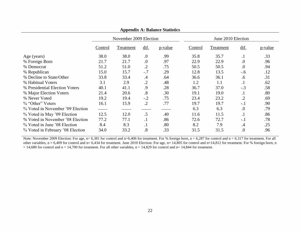
thanks”). As shown in Appendix A, randomization was successful. Differences between control
and treatment across a host of demographic and political variables (age, party registration, voting
history, nativity) were both substantively small and statistically insignificant.
Study Two: June 2010 Statewide Elections
The second field experiment was also conducted in San Mateo County, California, this
time during the June 2010 statewide primary elections. It included contested primary elections
for the Republican nominee for U.S. Senate, the Republican and Democratic nominees for
California Governor, and seven other statewide offices. It also included five statewide ballot
measures. There were 16,977,031 total registered voters eligible to vote in the election, and
5,654,813 cast a ballot (33% of registered). Ballot Measure 17—which dealt with auto insurance
regulation—was the closest race on the ballot. It lost by 1.9 percentage points (48.1% to 51.9%),
a margin of 202,940 votes. Although the final outcomes were not particularly close, there was
considerable interest in the gubernatorial contests. On the Democratic side, California Attorney
General Jerry Brown, well known from his days as former governor and former mayor of
Oakland, easily defeated a field that offered only token opposition. The Republican contest, in
contrast, saw ugly exchanges between the top two candidates, and set a record for the most
10
expensive campaign in California history, evidenced by the flooding of airwaves with competing
television advertisements. In the end, former EBay Chief Executive Meg Whitman defeated state
Insurance Commissioner Steve Poizner by double digits.7
We began the experiment with a list of registered voters for whom a telephone number
was provided by the voter at the time of registration. The list was prepared for randomization on
May 17, 2010, approximately three weeks before Election Day (June 8, 2010). Of the 338,378
registered voters in the county, we culled names of individuals who had provided a valid seven-
digit telephone number (128,471). We eliminated individuals who did not provide a unique
telephone number or who had sent an unsubscribe request in response to the November 2009 text
message. The firm Mobile Commons then determined which phone numbers belonged to cellular
phones. This left a pool of 34,281 valid cell phone numbers which we randomly divided into two
groups: (1) a control group (n = 17,150) which received no text message prior to Election Day;
and (2) a treatment group (n = 17,131) which received a message.
Paralleling the November 2009 experiment, text messages to the treatment groups were
sent on the Monday before Election Day (June 7, 2010). The text of the message was the same as
in the lower-salience election study, and we also randomized whether the message was
personalized. The messages were sent at 1:00 P.M. PST by the firm MessageMedia. The firm
also recorded which messages were not successfully delivered. The contact rate in the treatment
group was 99.99%; only 65 of the 17,131 messages bounced back as undelivered. Moreover,
because San Mateo County records the method of voting for each voter, we know if voters
participated in early voting and excluded those who did from the analysis (n=4,608), therefore
7 Whitman spent more than $71 million of her own money on the campaign and more than $88 million overall.
Poizner’s campaign was also mostly self-financed, spending more than $25 million. The record-level spending
continued in the gubernatorial general election for November 2010, with Whitman self-funding her campaign with a
record $140 million as of this writing.

11
reducing measurement error.
The resulting sample size is 29,673 (control: n=14,829; treatment: n=14,844). Of the
17,066 delivered texts, 452 individuals (less than 3%) sent replies: 123 were unsubscribe
requests, 41 were negative in nature, 185 were neutral, and 103 were positive. As shown in
Appendix A, randomization was successful.
Results and Implications
Main Effect of Cold Texts
November 2009. We first describe the main effects of the cold text messages for the
experiment conducted in the lower-salience election. After Election Day, we obtained an updated
voter file from the San Mateo County Registrar of Voters, which provided validated turnout
information for individuals in our treatment and control groups. As shown in the top row of the
top panel of Table 1, we observed a statistically significant treatment effect of the cold text
messages. In the control group, 253 of 6,156 individuals voted (3.95%). In the treatment group,
300 of 6,434 individuals voted (4.66%). This generates an intent-to-treat effect of 0.72
percentage points (s.e. = 0.36 percentage points), a statistically significant difference (p = 0.02,
one-tailed). We also conducted regression analysis via a linear probability model.8 We predict
voting with a treatment dummy and a host of demographic controls available in the voter file
(previous voting history in four elections, age, age squared, party identification).9 As shown in
8 We obtained similar results estimating a logistic regression model. The coefficient associated with the cold text
treatment is statistically different from zero at p=.01. We present estimates from the linear probability model for
ease of interpretation and because logistic regression may not be appropriate for analyzing randomized experiments
(Freedman 2008) and makes unneeded functional form assumptions (Angrist and Pischke 2009). Moreover,
interpreting interaction terms in limited dependent variable models introduces unneeded complexities (Ai and
Norton 2003). 9 A valid measure of age was not available for 56 registered voters in the November 2009 experiment and 56 voters
in the June 2010 experiment. We include age squared because the effect of age in this election was non-linear.
Previous research suggests that party identification explains variance in the dependent variable as Democrats are less
likely to vote than Republicans (e.g. Radcliff 1994; Citrin et al. 2003) and unaffiliated voters are less likely to vote
than partisans (Gerber and Green 2000).

12
the first column of Table 2, we obtain a similar intent-to-treat effect in terms of both size and
statistical significance (0.79 percentage points, s.e. = 0.34, p = 0.01).
[TABLE 1 ABOUT HERE]
[TABLE 2 ABOUT HERE]
How big is this effect in substantive terms? As a percentage of the baseline turnout rate
in the control group, cold texts increased turnout by 18.2%. In DS’s experiment, they found that
text messages increased turnout by 7.3% over their baseline rate. Running a simple probit
regression predicting turnout with the treatment dummy, we find the following coefficient
estimates: a = -1.76 (s.e. = 0.029) and b = 0.078 (s.e. = 0.039), producing a linear effect
equivalent to the approximately 0.7 percentage point effect noted above. However, assuming a
baseline turnout rate equivalent to DS’s 56.4% (a = 0.16), we find that the linear effect of the
treatment is 3 percentage points, identical to that observed by DS.
June 2010. We found an effect of similar size in the higher-salience election. As shown
in the top row of the bottom panel of Table 1, 8.9% (1,319/14,829) of individuals in the control
group voted compared to 9.8% (1,448/14,844) in the treatment group, producing an intent-to-
treat effect of 0.86 percentage points (s.e. = 0.34, p = 0.005). As we might expect, turnout rates
were over twice as large in the June 2010 election compared to the November 2009 election. As
shown in the third column of Table 2, the regression estimate is nearly the same (0.88 percentage
points, s.e. = 0.32, p = 0.003). This represents a 9.7% increase over the baseline turnout rate,
similar to the effect size observed by DS. Assuming a baseline turnout rate of 56.4%, we find the
linear effect of the treatment is 2 percentage points, slightly smaller than that observed by DS.
Thus, in two different electoral environments, we replicate DS’s main finding that noticeable
reminders are sufficient for increasing turnout. However, we strengthen the original results by

13
showing that they are robust to the elimination of auxiliary contact from the treatment messages.
We next explore whether different types of voters are contributing to the treatment effect in
different electoral contexts.
Heterogeneity by Voting History
November 2009. Voting history was available in the voter file for the four previous
elections: the May 2009 statewide special election, the November 2008 general election, the June
2008 primary election, and the February 2008 presidential primary. The November and
February10
elections had extremely high statewide turnout (79.4% and 57.7% of registered
voters, respectively) while the May and June elections had lower turnout levels (28.4% and
28.2%, respectively). We divided the sample into five natural subgroups:11
(1) habitual voters
who voted in each of the four elections (3.0% of the sample); (2) voters who only voted in the
November general presidential election (40.6%); (3) voters who only voted in the two major,
higher-turnout elections (21.0%); (4) voters who did not vote in any of the previous elections
(19.3%); and (5) all other voters (16.0%).12
As shown in the top panel of Table 1, we find an extremely large treatment effect among
habitual voters who voted in all of the prior elections, including those which featured low
turnout. Cold texts boosted turnout by 16.2 percentage points (p < 0.001) for these voters. For
the other subgroups examined, the estimated effects are substantively small and fail to reach
statistical significance. As shown in the second column of Table 2, compared to the baseline
group of “never voted,” the treatment effect was significantly greater for habitual voters (p <
10
The February 2008 presidential primary featured highly competitive contests for both major political parties. 11
As with our notion of “higher” and “lower” election salience, habitualness of voting is a relative construct.
However, for simplicity of interpretation, we separate voters into distinct categories and refer to them as “habitual
voters,” “major election voters,” and so forth. 12
The voter file provided by San Mateo County only included the voting history from the past four elections. On the
one hand, having data from earlier elections would better identify the various groups of voters. On the other hand,
given mobility of residents in the county, we would have substantial missing data for individuals who recently
moved into the county.

14
0.001). This is the case no matter which subgroup is selected as the baseline. Moreover, the
treatment effects among the other four subgroups are not significantly different from one
another. Noticeable reminders in this low-salience election were effective among voters who had
a high latent propensity to turnout—those individuals who seek to vote in every election, no
matter how minor. However, they had little effect on more casual voters that may be more
persuaded by social contact. These results are consistent with those of Arceneaux and Nickerson
(2009), who find that face-to-face efforts in low-salience elections have larger effects among
high-propensity voters than among low-propensity voters.
June 2010. We added turnout in November 2009 to our analysis, using five previous
elections to define the voting history of individuals in the higher salience experiment. We again
divided the sample into the five groups mentioned above. As shown in the bottom panel of Table
1, the effect of cold texts in the higher salience election was only positive and statistically
significant among casual voters—those who only voted in the presidential election or major
elections with high overall turnout. Among presidential election voters, the treatment effect was
1.0 percentage point (s.e. = 0.4, p = 0.005). Among major election voters, the treatment effect
was 2.3 percentage points (s.e. = 0.8, p = 0.002). Conversely, we did not observe a statistically
significant treatment effect among habitual voters (p = 0.81) and the effect size was negatively
signed (although the estimate cannot be distinguished from zero). Further, based on the
coefficient estimates in the fourth column of Table 2, the treatment effect among habitual voters
is significantly smaller than the treatment effects for both presidential election voters (5.4
percentage points, p = 0.03) and major election voters (6.8 percentage points, p = 0.01). Hence,
consistent with both NRT and contingent mobilization theory, casual voters are most affected by
reminders in higher-salience electoral environments, presumably because these voters are
15
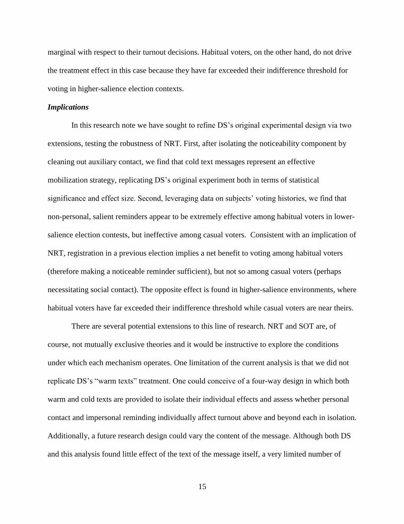
marginal with respect to their turnout decisions. Habitual voters, on the other hand, do not drive
the treatment effect in this case because they have far exceeded their indifference threshold for
voting in higher-salience election contexts.
Implications
In this research note we have sought to refine DS’s original experimental design via two
extensions, testing the robustness of NRT. First, after isolating the noticeability component by
cleaning out auxiliary contact, we find that cold text messages represent an effective
mobilization strategy, replicating DS’s original experiment both in terms of statistical
significance and effect size. Second, leveraging data on subjects’ voting histories, we find that
non-personal, salient reminders appear to be extremely effective among habitual voters in lower-
salience election contests, but ineffective among casual voters. Consistent with an implication of
NRT, registration in a previous election implies a net benefit to voting among habitual voters
(therefore making a noticeable reminder sufficient), but not so among casual voters (perhaps
necessitating social contact). The opposite effect is found in higher-salience environments, where
habitual voters have far exceeded their indifference threshold while casual voters are near theirs.
There are several potential extensions to this line of research. NRT and SOT are, of
course, not mutually exclusive theories and it would be instructive to explore the conditions
under which each mechanism operates. One limitation of the current analysis is that we did not
replicate DS’s “warm texts” treatment. One could conceive of a four-way design in which both
warm and cold texts are provided to isolate their individual effects and assess whether personal
contact and impersonal reminding individually affect turnout above and beyond each in isolation.
Additionally, a future research design could vary the content of the message. Although both DS
and this analysis found little effect of the text of the message itself, a very limited number of

16
messages have thus far been tested. SMS/MMS technology provides numerous opportunities to
provide more complex treatments (e.g. graphics and multimedia). For instance, one could
imagine showing voters their polling place with a Google map, thereby further reducing the
transaction costs involved in voting. Via further experimentation, scholars can gain a better
understanding of the mechanisms underlying political participation.

17
References
Ai, Chunron, and Edward C. Norton. 2003. “Interaction Terms in Logit and Probit Models.”
Economic Letters. 80: 123-129.
Angrist, Joshua D., and Jorn-Steffen Pischke. 2009. Mostly Harmless Econometrics: An
Empiricist's Companion. Princeton, NJ: Princeton University Press.
Arceneaux, Kevin, and David W. Nickerson. 2009. “Who is Mobilized to Vote? A Re-
Analysis of 11 Field Experiments.” American Journal of Political Science. 53(1): 1-16.
Citrin, Jack, Eric Schickler, and John Sides. “What if Everyone Voted? Simulating the Impact of
Increased Turnout in Senate Elections.” American Journal of Political Science. 47(1): 75-
90.
Dale, Allison, and Aaron Strauss. 2009. “Don’t Forget to Vote: Text Message Reminders as a
Mobilization Tool.” American Journal of Political Science. 53(4): 787-804.
Freedman, David A. 2008. “Randomization Does Not Justify Logistic Regression.” Statistical
Science. 23: 237-49.
Gerber, Alan S., and Donald P. Green. 2000. “The Effects of Canvassing, Telephone Calls, and
Direct Mail on Voter Turnout: A Field Experiment.” American Political Science Review.
94(3): 653-63.
Green, Donald P., and Alan S. Gerber. 2004. Get Out the Vote! How to Increase Voter Turnout.
Washington, DC: Brookings Institution Press.
Green, Donald P., and Alan S. Gerber. 2008. Get Out the Vote! How to Increase Voter Turnout.
Washington, DC: Brookings Institution Press. Second edition.
Nickerson, David W. 2006. “Volunteer Phone Calls Can Increase Turnout: Evidence from Eight
Field Experiments.” American Politics Research. 34(3): 271-92.

18
Nickerson, David W. 2007. “Does Email Boost Turnout?” Quarterly Journal of Political
Science. 2(4): 369-79.
Nickerson, David W., and Todd Rogers. 2010. “Do You Have a Voting Plan? Implementation
Intensions, Voter Turnout, and Organic Plan Making.” Psychological Science. 21(2):
194-199.
Radcliff, Benjamin. 1994. “Turnout and the Democratic Vote.” American Politics Research.
22(3): 259-276.

19
Table 1: The Effect of Cold Text Messages on Turnout
November 2009 Election
Sample Control (No Texts) Treatment (Cold Texts) Intent-to-Treat Effect
All Voters
(100.0%)
3.95%
(253/6,409)
4.66%
(300/6,434)
.72%
(s.e. = .36)
Habitual Voters
(3.0%)
25.9%
(52/201)
42.0%
(79/188)
16.2%
(s.e. = 4.7)
Pres. Election Voters
(40.6%)
1.4%
(36/2,573)
1.4%
(36/2,643)
.0%
(s.e. = .3)
Major Election Voters
(21.0%)
3.6%
(49/1,371)
4.1%
(55/1,328)
-.6%
(s.e. = .7)
Never Voted
(19.3%)
.9%
(11/1,232)
1.8%
(22/1,251)
.9%
(s.e. = .5)
“Other” Voters
(16.0%)
10.2%
(105/1,032)
10.5%
(108/1,024)
.4%
(s.e. = 1.3)
June 2010 Election
Sample Control (No Texts) Treatment (Cold Texts) Intent-to-Treat Effect
All Voters
(100.0%)
8.89%
(1,319/14,829)
9.75%
(1,448/14,844)
.86%
(s.e. = .34)
Habitual Voters
(1.1%)
60.1%
(104/173)
87.0%
(91/164)
-4.6%
(s.e. = 5.4)
Pres. Election Voters
(36.8%)
3.4%
(184/5,440)
4.3%
(238/5,492)
1.0%
(s.e. = .4)
Major Election Voters
(19.0%)
8.7%
(246/2,830)
11.0%
(310/2,816)
2.3%
(s.e. = .8)
Never Voted
(23.3%)
3.9%
(136/3,467)
4.0%
(137/3,441)
.1%
(s.e. = .5)
“Other” Voters
(19.7%)
22.2%
(649/2,919)
22.9%
(672/2,931)
.7%
(s.e. = 1.1)

20
Table 2: The Conditional Effect of Habitual Voting and Election Salience
Nov. 2009 Election June 2010 Election
Treatment (Cold Text Message) .0079*
(.0034)
.0075
(.0078)
.0088**
(.0032)
.0005
(.0066)
Habitual Voter .31***
(.011)
.23***
(.015)
.51***
(.015)
.53***
(.022)
Presidential Election Voter -.0015
(.0048)
.0024
(.0067)
-.0006
(.0043)
-.0106*
(.0060)
Major Election Voter .02***
(.0055)
.02**
(.0077)
.05***
(.0051)
.04***
(.0071)
“Other” Voter .08***
(.006)
.08***
(.008)
.17***
(.005)
.17***
(.007)
Treatment x Habitual Voter —— .16***
(.02)
—— -.05
(.03)
Treatment x Presidential Election Voter —— -.0079
(.0095)
—— .0086
(.0085)
Treatment x Major Election Voter —— -.0027
(.011)
—— .023*
(.010)
Treatment x “Other” Voter —— -.004
(.012)
—— .007
(.010)
Age .0027***
(.00068)
.0028***
(.00067)
.0021**
(.00068)
.0020**
(.00068)
Age Squared -.000022**
(.0000077)
-.000022**
(.0000077)
-.000004
(.000008)
-.000004
(.000008)
Republican .017**
(.005)
.017**
(.005)
.035***
(.005)
.035***
(.005)
Decline to State/Other .004
(.004)
.004
(.004)
-.016***
(.004)
-.016***
(.004)
Constant
-.059***
(.014)
-.060***
(.014)
-.023*
(.013)
-.019
(.013)
N 12787 12787 29617 29617
Adjusted R2
.09 .10 .10 .10 Note: ***p<.001; **p<.01; *p<.05 (two-tailed). Estimates from linear probability models. Baseline category is
“never voted.”

21
0
10
20
30
40
50
60
70
80
90
100
Nov. '07 Feb. '08 April '08 June '08 Nov. '08 May '09 Nov. '09 June '10
Turn
ou
t (%
)Figure 1: Turnout in San Mateo and Neighboring Counties
San Mateo San Francisco Santa Clara Santa Cruz
22
Appendix A: Balance Statistics
November 2009 Election June 2010 Election
Control Treatment dif. p-value Control Treatment dif. p-value
Age (years) 38.0 38.0 .0 .99 35.8 35.7 .1 .33
% Foreign Born 21.7 21.7 .0 .97 22.9 22.9 .0 .96
% Democrat 51.2 51.0 .2 .75 50.5 50.5 .0 .94
% Republican 15.0 15.7 -.7 .29 12.8 13.5 -.6 .12
% Decline to State/Other 33.8 33.4 .4 .64 36.6 36.1 .6 .31
% Habitual Voters 3.1 2.9 .2 .48 1.2 1.1 .1 .62
% Presidential Election Voters 40.1 41.1 .9 .28 36.7 37.0 -.3 .58
% Major Election Voters 21.4 20.6 .8 .30 19.1 19.0 .1 .80
% Never Voted 19.2 19.4 -.2 .75 23.4 23.2 .2 .69
% “Other” Voters 16.1 15.9 .2 .77 19.7 19.7 -.1 .90
% Voted in November ’09 Election 6.3 6.3 .0 .79
% Voted in May ’09 Election 12.5 12.0 .5 .40 11.6 11.5 .1 .86
% Voted in November ’08 Election 77.2 77.1 .1 .86 72.6 72.7 -.1 .78
% Voted in June ’08 Election 8.4 8.3 .1 .80 8.2 7.9 .4 .25
% Voted in February ’08 Election 34.0 33.2 .8 .33 31.5 31.5 .0 .96
Note: November 2009 Election: For age, n= 6,381 for control and n=6,406 for treatment. For % foreign born, n = 6,287 for control and n = 6.317 for treatment. For all
other variables, n = 6,409 for control and n= 6,434 for treatment. June 2010 Election: For age, n= 14,805 for control and n=14,812 for treatment. For % foreign born, n
= 14,680 for control and n = 14,700 for treatment. For all other variables, n = 14,829 for control and n= 14,844 for treatment.
Top Related