


Languages
Pages
Legal


University of Tennessee, Knoxville University of Tennessee, Knoxville
TRACE: Tennessee Research and Creative TRACE: Tennessee Research and Creative
Exchange Exchange
Masters Theses Graduate School
5-2018
Tennessee Row Crop Producer Survey on Willingness to Adopt Tennessee Row Crop Producer Survey on Willingness to Adopt
Best Management Practices Best Management Practices
Kelsey Michelle Campbell University of Tennessee
Follow this and additional works at: https://trace.tennessee.edu/utk_gradthes
Recommended Citation Recommended Citation Campbell, Kelsey Michelle, "Tennessee Row Crop Producer Survey on Willingness to Adopt Best Management Practices. " Master's Thesis, University of Tennessee, 2018. https://trace.tennessee.edu/utk_gradthes/5066
This Thesis is brought to you for free and open access by the Graduate School at TRACE: Tennessee Research and Creative Exchange. It has been accepted for inclusion in Masters Theses by an authorized administrator of TRACE: Tennessee Research and Creative Exchange. For more information, please contact [email protected].

To the Graduate Council:
I am submitting herewith a thesis written by Kelsey Michelle Campbell entitled "Tennessee Row
Crop Producer Survey on Willingness to Adopt Best Management Practices." I have examined
the final electronic copy of this thesis for form and content and recommend that it be accepted
in partial fulfillment of the requirements for the degree of Master of Science, with a major in
Agricultural and Resource Economics.
Christopher N. Boyer, Major Professor
We have read this thesis and recommend its acceptance:
Christopher D. Clark, Dayton M. Lambert, S. Aaron Smith
Accepted for the Council:
Dixie L. Thompson
Vice Provost and Dean of the Graduate School
(Original signatures are on file with official student records.)

Tennessee Row Crop Producer Survey on Willingness to Adopt Best
Management Practices
A Thesis Presented for the
Master of Science
Degree
The University of Tennessee, Knoxville
Kelsey Michelle Campbell
May 2018

ii
ACKNOWLEDGMENTS
Thanks for the United States Department of Agriculture National Institute of Food and
Agriculture and Food Research Initiative for funding this research (Competitive Grant Number
#2015-68007-23212).

iii
ABSTRACT
This thesis presents two separate studies focusing on best management practice (BMP) adoption
by row crop producers in Middle and West Tennessee. The objective of the first study is to
summarize results the survey. Survey topics included producer perceptions regarding the benefits
and costs from using no-tillage planting (no-till), cover crops, and irrigation water management
(IWM); respondent responsiveness to BMP cost-share payments; and producer demographic
information such as household income and age. The majority of survey respondents (87%) were
already planting using no-till, but only 28% knew they could receive a cost-share payment for
adopting no-till. Adoption of cover crops was about 29%, and no respondent indicated they have
adopted IWM.
Roughly half of producers were aware of United States Department of Agriculture cost-
share programs for cover crop adoption, and no producers knew cost-share payments for
adopting IWM are available. Producers were responsive to increases in cost-share payments
encouraging cover crop adoption; however, producer adoption of no-till and IWM was not
responsive to increases in cost-share payments. Data gathered from this survey indicates
Tennessee producers’ adoption and barriers to adoption of these BMPs, which could assist in
designing effective conservation policies.
The objective of the second study is to determine the effect of producer risk preference
and other factors such as cost-share payments on willingness to adopt cover crops and no-till
using a risk preference elicitation method. The same survey data was used. The results show that
producers are responsive to cost-share payments for cover crop adoption, but the likelihood a
producer would adopt no-till did not increase with higher cost-share payments. More risk averse
producers were less likely to adopt cover crops and no-till, as were those who did not believe the

iv
survey would influence future farm programs. Younger, college educated producers were more
risk tolerant than older producers without a 4-year degree. The results provide a better
understanding of producer risk preferences and will guide future studies in measuring and
assessing risk preferences of agricultural producers.

v
TABLE OF CONTENTS
INTRODUCTION .......................................................................................................................... 1 References ................................................................................................................................... 4
CHAPTER I 2017 MIDDLE AND WEST TENNESSEE ROW CROP PRODUCER SURVEY
RESULTS ....................................................................................................................................... 6
Abstract ....................................................................................................................................... 7 Introduction ................................................................................................................................. 8 Survey Data ................................................................................................................................. 9 Overview of Middle and West Tennessee Row Crop Operations ............................................ 11
Herbicide Resistant Weeds........................................................................................................ 12 No-Till ....................................................................................................................................... 12 Cover Crops............................................................................................................................... 13
Irrigation Water Management ................................................................................................... 14 Implications and Conclusions ................................................................................................... 16 References ................................................................................................................................. 18 Appendix A Tables and Figures ................................................................................................ 20
Appendix B Full Survey ............................................................................................................ 45 Appendix C Pre-Survey Postcard .............................................................................................. 52
Appendix D Survey Cover Letter.............................................................................................. 54 Appendix E Insert Included in Survey ...................................................................................... 56 Appendix F Survey Reminder Postcard .................................................................................... 58
CHAPTER II THE EFFECT OF PRODUCER RISK PREFERENCE ON WILLINGNESS TO
ADOPT COVER CROPS AND NO-TILL .................................................................................. 60
Abstract ..................................................................................................................................... 61
Introduction ............................................................................................................................... 62 Economic Framework ............................................................................................................... 65
Adoption ................................................................................................................................ 65
Risk ........................................................................................................................................ 66
Data ........................................................................................................................................... 68 Estimation.................................................................................................................................. 69 Variable Hypotheses ................................................................................................................. 72 Results ....................................................................................................................................... 74
Summary statistics ................................................................................................................. 74 Correlation coefficients and tests .......................................................................................... 76 WTA models.......................................................................................................................... 76
Risk aversion ......................................................................................................................... 78
Conclusions ............................................................................................................................... 79 References ................................................................................................................................. 81 Appendix G Tables and Figures ................................................................................................ 85
CONCLUSION ............................................................................................................................. 95 VITA ............................................................................................................................................. 97

vi
LIST OF TABLES
Table 1. Surveyed Producer Demographics .................................................................................. 21 Table 2. Number of Operations and Acreage Distribution for Relevant Operations by Crop...... 22
Table 3. 2017 USDA Reports of Tennessee Planted Acreage and Average Yield by Crop ......... 23 Table 4. Yield Summary for Survey Respondents........................................................................ 24 Table 5. Cost-share Program Awareness and Adoption of BMPs ................................................ 25 Table 6. Prevalence of Factors Used to Determine when to Irrigate ............................................ 26 Table 7. Amount of Water (in/ac) Applied to Corn, Cotton, and Soybeans ................................. 27
Table 8. Definition and Predicted Signs for the Independent Variables ....................................... 86 Table 9. Latent Constant Relative Risk Aversion Coefficients .................................................... 87 Table 10. Summary Statistics of Independent Variables (N = 344) ............................................. 88 Table 11. Correlation Coefficients of Residuals from Simultaneous Bivariate Probit and Tobit
Model ................................................................................................................................ 89 Table 12. Parameter Estimates and Significant Marginal Effects for the Probit Models and Tobit
Model (N = 344) ............................................................................................................... 90
vii
LIST OF FIGURES
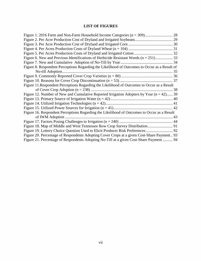
Figure 1. 2016 Farm and Non-Farm Household Income Categories (n = 309) ............................ 28 Figure 2. Per Acre Production Cost of Dryland and Irrigated Soybeans ...................................... 29
Figure 3. Per Acre Production Cost of Dryland and Irrigated Corn ............................................. 30 Figure 4. Per Acres Production Costs of Dryland Wheat (n = 104) ............................................. 31 Figure 5. Per Acres Production Costs of Dryland and Irrigated Cotton ....................................... 32 Figure 6. New and Previous Identifications of Herbicide Resistant Weeds (n = 251) ................. 33 Figure 7. New and Cumulative Adoption of No-Till by Year ..................................................... 34
Figure 8. Respondent Perceptions Regarding the Likelihood of Outcomes to Occur as a Result of
No-till Adoption ................................................................................................................ 35 Figure 9. Commonly Reported Cover Crop Varieties (n = 80) .................................................... 36 Figure 10. Reasons for Cover Crop Discontinuation (n = 53) ...................................................... 37
Figure 11.Respondent Perceptions Regarding the Likelihood of Outcomes to Occur as a Result
of Cover Crop Adoption (n = 238) ................................................................................... 38
Figure 12. Number of New and Cumulative Reported Irrigation Adopters by Year (n = 42)...... 39 Figure 13. Primary Source of Irrigation Water (n = 42) ............................................................... 40
Figure 14. Utilized Irrigation Technologies (n = 42) .................................................................... 41 Figure 15. Utilized Power Sources for Irrigation (n = 41) ............................................................ 42 Figure 16. Respondent Perceptions Regarding the Likelihood of Outcomes to Occur as a Result
of IWM Adoption ............................................................................................................. 43 Figure 17. Factors Posing Challenges to Irrigation (n = 240) ...................................................... 44
Figure 18. Map of Middle and West Tennessee Row Crop Survey Distribution ......................... 91 Figure 19. Lottery Choice Question Used to Elicit Producer Risk Preferences ........................... 92 Figure 20. Percentage of Respondents Adopting Cover Crops at a given Cost-Share Payment .. 93
Figure 21. Percentage of Respondents Adopting No-Till at a given Cost-Share Payment .......... 94

1
INTRODUCTION
Increases in water usage and climate uncertainties have led to growing concern regarding the
availability and preservation of adequate, clean, and fresh water sources for agricultural
production. Irrigated cropland is anticipated to expand globally to meet increasing demand for
food, fiber, and energy production (Rosegrant, Ringler, and Zhu, 2009; Schaible and Aillery,
2012). Furthermore, anticipated climate viability such as more frequent prolonged droughts
could negatively affect water availability and withdrawals as well as commodity prices and profit
margins. This future climate variability could also influence the adoption of irrigation for crop
production. The future availability of such water resources depends on how producers respond to
evolving these environmental concerns. For example, agricultural producers can adopt many
different best management practices (BMPs) that conserve water and soils. As such, it is valuable
to gain insights into who is willing to adapt their current agricultural production practices in
anticipation of an unclear future.
Farm conservation policy in the United States (US) started shifting in the late 1990s from
set-aside programs such as the Conservation Reserve Program to focus conservation efforts on
encouraging producers to adopt BMPs on working farmland (Cattaneo, 2003; Claassen,
Cattaneo, and Johansson, 2008). The Environmental Quality Incentives Program (EQIP) was
introduced in the Federal Agriculture Improvement and Reform Act of 1996 to partially
reimburse producers for voluntarily adopting BMPs on working farmland (Aillery, 2006;
Lichtenberg and Smith-Ramirez, 2011). The objective of working farmland programs is to
maximize environmental benefits per dollar spent by targeting land that would produce the
greatest environmental services from adopting BMPs without retiring farmland from production
(Claassen, Cattaneo, and Johansson, 2008; Reimer and Prokopy, 2014).
2
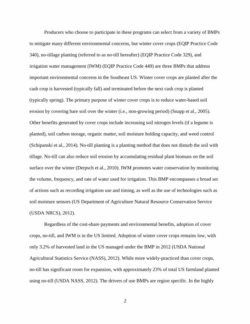
Producers who choose to participate in these programs can select from a variety of BMPs
to mitigate many different environmental concerns, but winter cover crops (EQIP Practice Code
340), no-tillage planting (referred to as no-till hereafter) (EQIP Practice Code 329), and
irrigation water management (IWM) (EQIP Practice Code 449) are three BMPs that address
important environmental concerns in the Southeast US. Winter cover crops are planted after the
cash crop is harvested (typically fall) and terminated before the next cash crop is planted
(typically spring). The primary purpose of winter cover crops is to reduce water-based soil
erosion by covering bare soil over the winter (i.e., non-growing period) (Snapp et al., 2005).
Other benefits generated by cover crops include increasing soil nitrogen levels (if a legume is
planted), soil carbon storage, organic matter, soil moisture holding capacity, and weed control
(Schipanski et al., 2014). No-till planting is a planting method that does not disturb the soil with
tillage. No-till can also reduce soil erosion by accumulating residual plant biomass on the soil
surface over the winter (Derpsch et al., 2010). IWM promotes water conservation by monitoring
the volume, frequency, and rate of water used for irrigation. This BMP encompasses a broad set
of actions such as recording irrigation use and timing, as well as the use of technologies such as
soil moisture sensors (US Department of Agriculture Natural Resource Conservation Service
(USDA NRCS), 2012).
Regardless of the cost-share payments and environmental benefits, adoption of cover
crops, no-till, and IWM is in the US limited. Adoption of winter cover crops remains low, with
only 3.2% of harvested land in the US managed under the BMP in 2012 (USDA National
Agricultural Statistics Service (NASS), 2012). While more widely-practiced than cover crops,
no-till has significant room for expansion, with approximately 23% of total US farmland planted
using no-till (USDA NASS, 2012). The drivers of use BMPs are region specific. In the highly

3
erodible Mississippi Portal, the USDA Region encompassing the majority of Middle and West
Tennessee, 33% of cropland acreage is planted using no-till or strip till (USDA Economic
Research Service (ERS), 2015) Since IWM includes a wide set of actions and technologies, there
is limited knowledge of the number of acres following each individual action and/or using each
technology that qualifies for the IWM program. However, USDA NRCS reported that over
450,000 acres received a cost-share payment for IWM in 2016 (USDA NRCS, 2017). In 2008,
7% of the total irrigated acres in the US were using more advanced irrigation technologies such
as surface drip, sub-surface drip, and low-flow micro sprinklers (USDA NASS, 2008).
This thesis presents two separate studies focusing on BMP adoption by row crop
producers in Middle and West Tennessee. The objective of the first study is to summarize results
from a 2017 survey of Middle and West Tennessee row crop producers. Survey topics included
producer perceptions regarding the benefits and costs associated with no-till, cover crops, and
IWM. Respondent responsiveness to BMP cost-share payments and producer demographic
information such as household income and age were also included as survey topics. Data
gathered from this survey will help us better understand how to design effective conservation
policies and get a better understanding of Tennessee producers’ use of these BMPs.
The objective of the second study is to determine the effect of producer risk preference
and other factors such as cost-share payments on willingness to adopt (WTA) cover crops and
no-till using a risk preference elicitation method to measure producer risk preferences. Data from
a 2017 survey of Middle and West Tennessee row crop producers was once again used. The
results provide a better understanding of producer risk preferences and can guide future studies
to measure and assess producer risk preferences.

4
References
Aillery, M. “Contrasting Working-Land and Land Retirement Programs.” Economic Brief 4,
U.S. Department of Agriculture, Economic Research Service, Washington, DC, 2006.
Internet site: http://www.ers.usda.gov/publications/eb-economic-brief/eb4.aspx.
Cattaneo, A. “The Pursuit of Efficiency and its Unintended Consequences: Contract,
Withdrawals in the Environmental Quality Incentives Program.” Review of Agricultural
Economics 25(2003):449-469.
Claassen, R., A. Cattaneo, and R. Johansson. “Cost-Effective Design of Agri-Environmental
Payment Programs: U.S. Experience in Theory and Practice.” Ecological Economics
65(2008):737-752.
Derpsch, R., T. Friedrich, A. Kassam, and L. Hongwen. “Current Status of Adoption of No-Till
Farming in the World and Some of its Main Benefits.” International Journal of
Agricultural & Biological Engineering 3(1)(2010):1-25.
Lichtenberg, E., and R. Smith-Ramírez. “Slippage in Conservation Cost Sharing.” American
Journal of Agricultural Economics 93(2011):113–129. doi: 10.1093/ajae/aaq124.
Reimer, A.P, and L.S. Prokopy. “One Federal Policy, Four Different Policy Contexts: An
Examination of Agri-Environmental Policy Implementation in the Midwestern United
States.” Land Use Policy 38(2014):605–614.
Rosegrant M.W., C. Ringler, T. Zhu. “Water for Agriculture: Maintaining Food Security Under
Growing Scarcity.” Annual Review of Environment and Resources. 34(2009)205-22.
Schaible G, M. Aillery. “Water Conservation in Irrigated Agriculture: Trends And Challenges In
The Face Of Emerging Demands.” USDA-ERS Economic Information Bulletin 99. 2012.
Schipanski, M.E., M. Barbercheck, M.R. Douglas, D.M. Finney, K. Haider, J.P. Kayne, A.R.
Kemanian, D.A. Mortensen, M.R. Ryan, J. Tooker. “A Framework for Evaluating
Ecosystem Services Provided by Cover Crops in Agroecosystems.” Agricultural Systems
125(2014):12-22.
Snapp, S.S., S.M. Swinton, R. Labarta, D. Mutch, J.R. Black, R. Leep, J. Nyiraneza, and K.
O’Neil. “Evaluating Cover Crops for Benefits, Costs, and Performance within Cropping
System Niches.” Agronomy Journal 97(2005):322-332.
U.S. Department of Agriculture, National Agricultural Statistics Service (USDA NASS).
Census of Agriculture, 2007. Washington, DC: 2008.
U.S. Department of Agriculture, National Agricultural Statistics Service (USDA NASS). Census
of Agriculture, 2012. Washington, DC: 2012. Internet site:

5
https://www.agcensus.usda.gov/Publications/2012/Full_Report/Volume_1,_Chapter_1_St
ate_Level/Tennessee/st47_1_055_055.pdf
U.S. Department of Agriculture, Natural Resources Conservation Service. Washington, DC:
Natural Resource Conservation Service, Environmental Quality Incentives Program
(EQIP). 31 May 2017. Available online at:
http:http://www.nrcs.usda.gov/Internet/NRCS_RCA/reports/fb08_cp_eqip.html

6
CHAPTER I 2017 MIDDLE AND WEST TENNESSEE ROW CROP PRODUCER
SURVEY RESULTS

7
Abstract
This chapter presents a summary of results from a 2017 survey of Middle and West Tennessee
row crop producers. Data gathered from this survey will further our understanding of the design
of effective conservation policies and of Tennessee producers’ use of no-till, cover crops, and
irrigation water management (IWM). Most of the 344 survey respondents (87%) planted with
no-till in 2016, which is considerably higher than the 29% of respondents who planted cover
crops in 2016. Common reasons producers cited for not growing cover crops included expense
and increased planting difficulty. All respondents were asked about factors posing difficulties to
irrigating on their operation. The most common barriers to irrigation were installation expense,
and field size and shape. Surveyed producers largely believed that no-till and cover crops would
benefit soil quality/health, reduce erosion, and improve water quality. However, they were less
sure about the likelihood of no-till and cover crops increasing yields and reducing yield
variability.
Keywords: cost sharing, no-till, cover crops, irrigation water management, survey, Tennessee

8
Introduction
United States (US) farm conservation programs primarily concentrate on promoting the use of
best management practices (BMPs) on working farmland (Cattaneo, 2003; Claassen, Cattaneo,
and Johansson, 2008). Programs such as the Environmental Quality Incentives Program (EQIP)
offer partial reimbursement for voluntarily adopted BMPs on working farmland (Aillery, 2006).
Qualified producers can choose from a variety of BMPs to mitigate many different
environmental issues such as soil erosion, soil carbon storage, organic matter, soil moisture
holding capacity, water conservation, and weed control (Schipanski et al., 2014).
In Tennessee, winter cover crops (EQIP Practice Code 340), no-tillage planting (referred
to as no-till hereafter) (EQIP Practice Code 329), and irrigation water management (IWM)
(EQIP Practice Code 449) address important environmental concerns (US Department of
Agriculture (USDA) Natural Resource Conservation Service (NRCS), 2017). Winter cover crops
are planted after the cash crop is harvested (typically fall) and terminated before the next cash
crop is planted (typically spring). This BMP can reduce water-based soil erosion by covering
bare soil over the winter (i.e., non-growing period) as well as increase soil nitrogen levels (if a
legume cover crop is planted), soil carbon storage, organic matter, soil moisture holding
capacity, and weed control (Snapp et al., 2005; Schipanski et al., 2014). No-till planting does not
disturb the soil with tillage, reducing soil erosion by accumulating residual plant biomass on the
soil surface over the winter (Derpsch et al., 2010). The purpose of IWM is to promote water
conservation by monitoring the volume, frequency, and rate of water used for irrigation. IWM
includes a wide set of actions such as recording irrigation use and timing as well as the use of
technologies such as soil moisture sensors (USDA NRCS, 2012).

9
Adoption of cover crops, no-till, and IWM in the US has been low despite the availability
of cost-share payments and potential environmental benefits. Winter cover crop adoption in the
US is around 3.2% of harvested farmland in 2012 (USDA National Agricultural Statistics
Service (NASS), 2012). While more widely-adopted than winter cover crops, no-till still has
significant room for expansion, with approximately 23% of total US crop land planted using no-
till in 2012 (USDA NASS, 2012). Since IWM includes a wide set of actions and technologies,
there is limited knowledge of the number of acres following each individual action and/or using
each technology that qualifies for the IWM program. However, USDA NRCS reported that over
450,000 acres received a cost-share payment for IWM in 2016 (USDA NRCS, 2017). In 2008,
7% of the total irrigated acres in the US were using more advanced irrigation technologies such
as surface drip, sub-surface drip, and low-flow micro sprinklers (USDA NASS, 2008).
The objective of this chapter is to present results from a 2017 survey of Middle and West
Tennessee row crop producers (Appendix B), offering insights into perceptions regarding the
benefits and costs associated with no-till, cover crops, and IWM, responsiveness to BMP cost-
share payments, and producer demographic information such as household income and age. Data
gathered from this survey will inform policy makers and Extension agents on use of BMPs in
Middle and West Tennessee.
Survey Data
Following Dillman’s (2007) mail survey total design method recommendations, a postcard
(Appendix C) was first mailed on January 26, 2017 to inform row crop producers that they
would soon be receiving the full Middle and West Tennessee row crop producer survey. The first
round of mail surveys was sent out on February 8, 2017. A prepaid postage envelope was
included, as well as a cover letter (Appendix D) explaining the purpose of the survey and an

10
insert (Appendix E) detailing the benefits and requirements of winter cover crops, no-till, and
IWM. A reminder postcard (Appendix F) was sent out on February 17, 2017, followed by a
second round of questionnaires on March 8, 2017. A third and final round of surveys was mailed
in July 2017. The survey was initially mailed to 5,184 addresses of individuals who received
Farm Service Agency (FSA) payments from 2012-2016.Declines to participate, undeliverable
addresses, and replies that the recipient does not farm reduced the survey pool to 3,84l. A total of
344 responses to the mail survey were received, resulting in a 9% response rate.
The survey included six sections, with the first including questions about acreage farmed,
crop yields, and production costs. The second, third, and fourth sections covered questions on
no-till, cover crops, and IWM; respectively. The fifth and sixth sections of the survey solicited
information on producer demographics including age, education, and income.
The average age of survey respondents was 64 years old, which is slightly older than the
average age of principal operators in the state (59 years old in 2012) (USDA NASS, 2012).
Approximately 41% of producers surveyed had a college degree or equivalent. Roughly half of
respondents had a total of farm and non-farm income for 2016 of less than $99,999, and roughly
5% of respondents reported their 2016 income to be $500,000 or above (Figure 1). Over half of
respondents, 184 of 319 (58%), were enrolled in crop insurance in 2016 (Table 1). According to
USDA Risk Management Agency (RMA) reports for Tennessee, 82% of corn acreage, 91% of
cotton acreage, 83% of soybean acreage, and 76% of wheat acreage were insured in 2016
(USDA RMA, 2016). One possible explanation of our result is the difference between number of
respondents and the percentage of acres.

11
Overview of Middle and West Tennessee Row Crop Operations
Soybeans were the most planted crop among respondents, followed by corn, wheat, and then
cotton (Table 2), which is consistent with the prevalence of planted acreage by crop statewide
(USDA NASS, 2017) (Table 3). The majority of soybeans were produced on dryland acres with
the average size of 388 acres of soybeans per participating operation (Table 2) and average yield
of 43 bushels per acre (Table 4). For producers who did irrigate soybeans, the average operation
size was 483 acres (Table 2), and they reported an average yield of 55 bushels per acre (Table 4).
Most respondents reported that their dryland soybean costs of production were between $100 and
$199 per acre, excluding any land rent costs (Figure 2). A majority of those irrigating their
soybeans said their production costs were $200 to $299 per acre (Figure 2).
Dryland corn was produced by 152 respondents in 2016, and 33had irrigated corn acreage
(Table 2). Of operations with dryland corn, the average dryland corn acreage was 267 acres, and
irrigated corn farms averaged 328 acres (Table 2). Yields averaged 140 bushels per acre and 197
bushels per acre for dryland and irrigated corn, respectively (Table 4). Production costs of
dryland corn were most commonly reported between $300 and $399 per acre, while irrigated
corn costs of production were said to be closer to between $400 and $499 per acre (Figure 3).
Less than 100 respondents (96 producers) said they produced dryland wheat, with the
average size of a dryland wheat operation being 232 acres (Table 2). Only six respondents
reported growing irrigated wheat in 2016 with an average farm size of 432 acres (Table 2).
Those who were growing irrigated wheat were likely double cropping, with irrigation
technologies primarily installed for the spring planted crop. Dryland wheat yield averaged 67
bushels per acre, and the six respondents who had irrigated wheat acreage reported an average
yield of 78 bushels per acre (Table 4). The cost of production for dryland wheat was between

12
$150 and $199 per acre for 35% of the respondents and between $200 and $249 per acre for 30%
of the respondents (Figure 4). Irrigated costs of production for wheat was not collected.
Forty-nine producers surveyed said they grew dryland cotton, and 10 irrigated cotton in
2016 (Table 2). Average acreage for dryland cotton was 372 acres, while average irrigated cotton
acreage was higher at 460 acres (Table 2). Survey respondents reported an average yield of 909
pounds per acre for dryland cotton and 1,058 pounds per acre for irrigated cotton (Table 4).
Production costs for dryland cotton ranged from $300 to $399 per acre for 42% of the
respondents, and irrigated cotton costs were reported to be less than $399 per acre for the
majority of question respondents (Figure 5).
Herbicide Resistant Weeds
Most respondents (69%) had identified herbicide resistant weeds on their operation. The earliest
reported herbicide resistant weeds are in 1999, with a sharp increase in cases reported around
2010 (Figure 6). With the majority of producers reporting the presence of herbicide resistant
weeds on their operation, it is likely this will continue to be a topic of growing concern and
interest.
No-Till
Only 21% of the survey respondents said they knew the cost of no-till could be partially
reimbursed by the USDA NRCS. Of the respondents who were aware of the existence of a cost-
share program, only 16 (~33%) reported receiving a cost-share payment for no-till (Table 5).
However, 260 out of 300 producer responses to the survey (87%) said they planted with no-till
(Table 4), which is higher than USDA NASS’s (2016) report that 75.9% of Tennessee acreage
was planted using no-till in 2016. The adoption of no-till was reported to be in as early as 1948

13
and as recent as 2015 (Figure 7). Respondents using the BMP reported having an average of 605
no-till acres (Table 5).
Respondents were asked about their opinion regarding the likelihood of a variety of
outcomes occurring as a result of using no-till on their operation. Queried outcomes were
increased yield, reduced yield variability, retained soil moisture, reduced erosion, reduced cost,
weed control, improved soil quality/health, improved water quality, and increased management
burden. On average, respondents seemed to believe there was a high likelihood of improved soil
health and erosion reduction as a result of no-till. Those surveyed were less optimistic about no-
till’s ability to reduce weeds, increase yield, and reduce yield variability (Figure 8).
Cover Crops
Approximately half of the respondents indicated they were aware the costs of cover crops may
be partially reimbursed by the NRCS. Of the respondents who were aware a cover crop cost-
share program existed, 53 (49%) indicated they had previously received a cost-share payment for
cover crops (Table 5).
University of Tennessee Extension reported that 22% of Tennessee row crop acreage was
planted after a cover crop in 2015 (University of Tennessee Institute of Agriculture, 2015).
Based on the 2017 survey, 29% of the respondents said they planted cover crops in 2016, 22%
said they did not plant cover crops in 2016 but had previously, and 49% said they had never used
cover crops (Table 5). Cover crop usage averaged 269 acres of land per participating operation
(Table 4). Several cover crop varieties were reportedly used by surveyed producers, with 65
respondents saying they planted wheat, 43 planted rye, 29 planted radish, 28 planted clover, 15
planted oats, ten planted turnips, six planted vetch, and three planted rapeseed (Figure 9).

14
Respondents who had previously grown cover crops but stopped using the BMP were
asked what prompted the discontinuation. Reasons surveyed included too expensive, made
planting difficult, reduced yields, too complicated, and tough to terminate. The most common
reasons for stopping cover crop application were reported to be increased planting difficulty,
with 26 responses and too expensive, with 24 responses (Figure 10). Respondents were permitted
to select more than one reason for stopping the use of the BMP.
Respondents were asked about their perception of the likelihood of increased yield,
reduced yield variability, retained soil moisture, reduced erosion, increased profit, weed control,
improved soil quality/health, improved water quality, and increased planting difficulty to occur
from the planting of cover crops. Producers largely believed reduced erosion, improved soil
quality/health, and improved water quality were likely to occur as a result of using cover crops.
A high percentage of producers said they had no idea of the impact cover crop adoption would
have on increased yield or reduced yield variability (Figure 11).
Irrigation Water Management
Only 30 out of 274 respondents (11%) said they knew the costs of IWM may be partially
reimbursed by the USDA, substantially fewer than those who were aware of no-till and cover
crop cost-share payment programs. Of the 30 respondents who knew of the cost-share program
availability, none reported ever receiving a cost-share for IWM (Table 5).
Though none reported receiving cost-share assistance for IWM, 42 out of 273
respondents to the question (15%) reported that they irrigated (Table 5), with the earliest report
of irrigation being 1988 and the most recent being 2017 (Figure 12). In the state of Tennessee,
146,932 of 823,932 (18%) acres on operations using irrigation to some extent were irrigated in
2013, but not necessarily using more advanced IWM technologies (USDA NASS, 2013). Based

15
on this figure roughly 5% of all Tennessee row crop acreage is irrigated (USDA FSA, 2017)
Knowledge regarding the number of acres following each individual action and/or using each
technology that qualifies for the IWM program is limited, as IWM includes a wide variety of
actions and technologies.
Producers who irrigated were asked about their primary water source for irrigation, with
40 respondents saying a well was their primary source with an average depth of about 200 feet.
No irrigators reported having a river/stream or lake as their primary irrigation water source, and
two respondents said their irrigation water source was a farm pond (Figure 13). Center pivot was
by far the most common type of irrigation system among producers surveyed, with 38 of the 42
irrigators (90%) using the practice, followed by furrow (three respondents), traveling gun (two
respondents), and subsurface drip (2 respondents) (Figure 14). Respondents could select more
than one irrigation technology if multiple were in use on their operation. The power source used
for irrigation is primarily electricity (31 of the 42 total irrigators or 74%), followed by diesel
(74%) and natural gas (5%) (Figure 15).
Respondents who irrigated were asked to select the method(s) they used to determine
when to irrigate from a menu of options consisting of water balance, soil moisture sensors, plant
status, consultant, growth stage, neighbor irrigated, and a schedule. Growth stage, soil moisture
sensors, and plant status were the most frequently reported factors in the irrigation timing
decision (Table 6). The 42 respondents who irrigated were asked how much water (inches per
acre) they usually applied when irrigating corn, cotton, and soybeans (Table 7). Corn was the
most commonly irrigated crop, and 27 of the 36 reporting corn irrigators (75%) said they apply
0.25” – 0.50” inches per acre when they irrigate the crop. Of the 11 respondents who irrigated
cotton, roughly half apply 0.25” – 0.50” inches per acre, with another 45% applying 0.51” –

16
0.99” inches per acre. There are 35 question respondents reporting irrigating soybeans, with
66% applying between 0.25” – 0.50” inches per acre per application.
Respondents who irrigated were asked their opinion on the likelihood of achieving higher
yields, reduced yield variability, increased profit, securing an operating loan, and lower crop
insurance costs to occur from using IWM on their farm. Respondents were confident that the use
of IWM would increase yields, reduce yield variability, and increase profit. However, few
producers thought IWM would increase the likelihood of securing an operating loan or lower
their crop insurance costs (Figure 16).
All respondents, including non-irrigators, were asked a question regarding the challenges
to irrigating on their operation. Producers were offered a menu of potential challenges consisting
of field slope, field shape, water quality, water availability, field size, installation expense,
existing debt, loan availability, time and effort needed, uncertain commodity prices, and
uncertain energy costs. Respondents were permitted to select more than one factor they
considered a challenge to irrigation. 240 responded to the question, and the most commonly cited
challenges were installation expense (149 responses), field size (143 responses), and field shape
(137 responses) (Figure 17).
Implications and Conclusions
Most producers (87%) reported using no-till in 2016, but only 21% of respondents were
aware the USDA may partially reimburse the costs of no-till adoption, and 28% of those who
were aware of the program reported receiving a USDA cost-share payment. Just under one third
(29%) of survey respondents planted cover crops in 2016, and an additional 22% had planted
cover crops in the past but did not in 2016. Common reasons cited for the discontinuation of
cover crop planting included increased planting difficulty and too expensive. About half (52%)
17
of respondents were aware the costs of cover crop adoption may be partially reimbursed by the
USDA, and roughly half of those who knew USDA cost-share assistance was available reported
participating in the cost-share program. Increases in cost-share amount offered for cover crop
adoption were found to consistently increase adoption rates of the BMP. Knowledge of IWM
USDA cost-share assistance was low, with only 11% of respondents reporting awareness.
Furthermore, no producers reported having ever received USDA cost-share assistance for IWM.
Data gathered from this survey will help us further understand how to design effective
conservation policies and to get a better understanding of Tennessee producers’ use of no-till,
cover crops, and IWM.
Based on survey results, no-till adoption rates do not dramatically improve given higher
cost-share payments. As few producers were aware USDA cost-share assistance was available
for IWM, increased program advertising may improve adoption rates in the region.

18
References
Aillery, M. “Contrasting Working-Land and Land Retirement Programs.” Economic Brief 4,
U.S. Department of Agriculture, Economic Research Service, Washington, DC, 2006.
Internet site: http://www.ers.usda.gov/publications/eb-economic-brief/eb4.aspx.
Cattaneo, A. “The Pursuit of Efficiency and its Unintended Consequences: Contract,
Withdrawals in the Environmental Quality Incentives Program.” Review of Agricultural
Economics 25(2003):449-469.
Claassen, R., A. Cattaneo, and R. Johansson. “Cost-Effective Design of Agri-Environmental
Payment Programs: U.S. Experience in Theory and Practice.” Ecological Economics
65(2008):737-752.
Derpsch, R., T. Friedrich, A. Kassam, and L. Hongwen. “Current Status of Adoption of No-Till
Farming in the World and Some of its Main Benefits.” International Journal of
Agricultural & Biological Engineering 3(1)(2010):1-25.
Dillman, D. Mail and Internet Surveys: The Tailored Design Method. Hoboken, New Jersey:
John Wiley & Sons, 2007.
Schipanski, M.E., M. Barbercheck, M.R. Douglas, D.M. Finney, K. Haider, J.P. Kayne, A.R.
Kemanian, D.A. Mortensen, M.R. Ryan, and J. Tooker. “A Framework for Evaluating
Ecosystem Services Provided by Cover Crops in Agroecosystems.” Agricultural Systems
125(2014):12-22.
Snapp, S.S., S.M. Swinton, R. Labarta, D. Mutch, J.R. Black, R. Leep, J. Nyiraneza, and K.
O’Neil. “Evaluating Cover Crops for Benefits, Costs, and Performance within Cropping
System Niches.” Agronomy Journal 97(2005):322-332.
U.S. Department of Agriculture, Farm Service Agency (USDA FSA). Crop Acerage Data, 2016.
Washington, DC: 2017. Internet site: https://www.fsa.usda.gov/news-
room/efoia/electronic-reading-room/frequently-requested-information/crop-acreage-
data/index
U.S. Department of Agriculture, National Agricultural Statistics Service (USDA NASS). Census
of Agriculture, 2012. Washington, DC: 2012. Internet site:
https://www.agcensus.usda.gov/Publications/2012/Full_Report/Volume_1,_Chapter_1_St
ate_Level/Tennessee/st47_1_055_055.pdf
U.S. Department of Agriculture, National Agricultural Statistics Service (USDA NASS). Census
of Agriculture, 2013. Washington, DC: 2012. Internet site:
https://www.agcensus.usda.gov/Publications/2012/Online_Resources/Farm_and_Ranch_I
rrigation_Survey/fris13_1_002_002.pdf
U.S. Department of Agriculture, National Agricultural Statistics Service (USDA NASS). 2017
State Agricultural Overview: Tennessee. Washington, DC: 2017. Internet site:

19
https://www.nass.usda.gov/Quick_Stats/Ag_Overview/stateOverview.php?state=TENNE
SSEE
U.S. Department of Agriculture, Natural Resources Conservation Service. Washington, DC:
Natural Resource Conservation Service, Environmental Quality Incentives Program
(EQUIP). 31 May 2017. Available online at:
http:http://www.nrcs.usda.gov/Internet/NRCS_RCA/reports/fb08_cp_eqip.html>
U.S. Department of Agriculture, National Agricultural Statistics Service (USDA NASS).
Census of Agriculture, 2007. Washington, DC: 2008.
U.S. Department of Agriculture, Risk Management Agency (USDA RMA). Summary of
Business Reports and Data, 2016. Washington, DC: 2016.
University of Tennessee Institute of Agriculture. “Cover Crop Considerations for this Fall.”
UTcrops News Blog (2015). Internet site: http://news.utcrops.com/2015/08/cover-crop-
considerations-for-this-fall/
Wade, T., R. Claassen, and S. Wallander. Conservation-Practice Adoption Rates Vary Widely by
Crop and Region, EIB-147, U.S. Department of Agriculture, Economic Research Service,
December 2015.

20
Appendix A Tables and Figures

21
Table 1. Surveyed Producer Demographics
Factor Value
Age (average in years) 64
College degree (percent holding) 41%
Crop insurance (percent enrolled) 57.68%

22
Table 2. Number of Operations and Acreage Distribution for Relevant
Operations by Crop
Crop Number of
operations Mean (acres)
Minimum
(acres)
Maximum
(acres)
Soybeans – dry 238 388 3 4,000
Soybeans – irrigated 30 483 50 2,500
Corn – dry 152 267 1 3,080
Corn – irrigated 33 328 50 1,800
Wheat – dry 96 232 2 1,900
Wheat – irrigated 6 432 35 1,600
Cotton – dry 49 372 1 2,000
Cotton – irrigated 10 460 24 2,000

23
Table 3. 2017 USDA Reports of Tennessee Planted Acreage and Average
Yield by Crop
Crop Planted Acres Average Yield
Soybeans 1,580,048 50 (bu/acre)
Corn 822,142 171 (bu/acre)
Wheat 348,160 70 (bu/acre)
Cotton 251,959 1,031 (lb/acre)
Sources: USDA NASS, 2017 & USDA FSA, 2017

24
Table 4. Yield Summary for Survey Respondents
Crop Minimum Mean Maximum
Dryland corn (bu/ac) 107 (n = 150) 140 (n = 145) 175 (n = 155)
Irrigated corn (bu/ac) 171 (n = 34) 197 (n = 35) 236 (n = 35)
Dryland cotton (lbs/ac) 726 (n = 39) 909 (n = 39) 1107 (n = 41)
Irrigated cotton (lbs/ac) 1046 (n = 7) 1058 (n = 7) 1356 (n = 7)
Dryland soybeans (bu/ac) 50 (n = 208) 43 (n = 196) 82 (n = 216)
Irrigated soybeans (bu/ac) 46 (n = 30) 55 (n = 29) 67 (n = 30)
Dryland wheat (bu/ac) 64 (n = 98) 67 (n = 93) 90 (n = 101)
Irrigated wheat (bu/ac) 65 (n = 1) 78 (n = 1) 91 (n = 1)

25
Table 5. Cost-share Program Awareness and Adoption of BMPs
No-till Cover crops IWM*
Aware of USDA cost-share assistance 21% (n = 298) 52% (n = 307) 11% (n = 274)
Received cost-share assistance (of those
who were aware of program) 28% (n = 57) 49% (n = 108) 0% (n = 30)
Received cost-share assistance (of all
respondents) 5% (n = 344) 15% (n = 344) 0% (n = 344)
Currently using BMP 87% (n = 300) 28% (n = 300) -
Used BMP in past but did not in 2016 - 22% (n = 300) -
Have never used BMP - 49% (n = 300) -
Acreage enrolled in BMP (average) 605 (n = 215) 268 (n = 82) - *Irrigation water management

26
Table 6. Prevalence of Factors Used to Determine
when to Irrigate
Factor Percentage Citing (n = 42)
Water balance 21%
Growth stage 43%
Soil moisture sensors 48%
Neighbor irrigated 14%
Plant status 52%
A schedule 0%
Consultant 21%

27
Table 7. Amount of Water (in/ac) Applied to Corn, Cotton, and Soybeans
Number of Respondents
Amount Applied Per
Application (in/ac)
Corn (n = 36) Cotton (n = 11) Soybeans (n = 35)
Less than 0.25” 6% 0% 11%
0.25”-0.50” 75% 45% 66%
0.51”-0.99” 14% 45% 17%
1-1.49” 0% 0% 0%
1.5-1.99” 3% 0% 3%
2-2.49” 3% 9% 3%
More than 2.49” 0% 0% 0%

28
Figure 1. 2016 Farm and Non-Farm Household Income Categories (n = 309)
0%
10%
20%
30%
40%
50%
60%
< $99,999 $100,000 -
$299,999
$300,000 -
$499,999
$500,000 -
$699,999
$700,000 -
$999,999
> $1
million
Per
cen
tage
of
Res
pon
den
ts

29
Figure 2. Per Acre Production Cost of Dryland and Irrigated Soybeans
0%
10%
20%
30%
40%
50%
60%P
erce
nta
ge
of
Res
pon
den
ts
Dryland Soybeans
(n = 234)
Irrigated Soybeans
(n = 32)

30
Figure 3. Per Acre Production Cost of Dryland and Irrigated Corn
0%
10%
20%
30%
40%
50%
60%P
erce
nta
ge
of
Res
pon
den
ts
Dryland Corn
(n = 165)
Irrigated Corn
(n = 38)

31
Figure 4. Per Acres Production Costs of Dryland Wheat (n = 104)
0%
5%
10%
15%
20%
25%
30%
35%
40%
<$149 $150-
$199
$200-
$249
$250-
$299
>$300
Per
cen
tage
of
Res
pon
den
ts

32
Figure 5. Per Acres Production Costs of Dryland and Irrigated Cotton
0%
10%
20%
30%
40%
50%
60%
70%P
erce
nta
ge
of
Res
ponden
ts
Dryland Cotton (n = 48)
Irrigated Cotton (n = 9)

33
Figure 6. New and Previous Identifications of Herbicide Resistant Weeds (n = 251)
0%
10%
20%
30%
40%
50%
60%
1999
2000
2001
2002
2003
2004
2005
2006
2007
2008
2009
2010
2011
2012
2013
2014
2015
2016
Per
cen
tage
of
Res
pon
den
ts
Year
Cumulative
New

34
Figure 7. New and Cumulative Adoption of No-Till by Year
0%
10%
20%
30%
40%
50%
60%
70%
1948
1952
1956
1960
1964
1968
1972
1976
1980
1984
1988
1992
1996
2000
2004
2008
2012
Per
cen
tage
of
Res
pon
den
ts
Cumulative
New

35
Figure 8. Respondent Perceptions Regarding the Likelihood of Outcomes to Occur as a
Result of No-till Adoption
0%
10%
20%
30%
40%
50%
60%
70%
80%
90%
100%P
erce
nta
ge
of
Res
pon
den
ts R
eport
ing
75-100% likely
51-75% likely
50/50% likely
25-49% likely
0-25% likely
No Idea

36
Figure 9. Commonly Reported Cover Crop Varieties (n = 80)
0
5
10
15
20
25
30
35
40
45
50N
um
ber
of
Res
pon
den
ts

37
Figure 10. Reasons for Cover Crop Discontinuation (n = 53)
0%
10%
20%
30%
40%
50%
60%
Made
planting
difficult
Too
expensive
Other Tough to
terminate
Too
complicated
Reduced
yields
Per
cen
tage
of
Res
pon
den
ts

38
Figure 11. Respondent Perceptions Regarding the Likelihood of Outcomes to Occur as a
Result of Cover Crop Adoption (n = 238)
0%
10%
20%
30%
40%
50%
60%
70%
80%
90%
100%P
erce
nta
ge
of
Res
pon
den
ts R
eport
ing
75-100% likely
51-75% likely
50/50% likely
25-49% likely
0-25% likely
No Idea

39
Figure 12. Number of New and Cumulative Reported Irrigation Adopters by Year (n = 42)
0
5
10
15
20
25
30
35
40
45
1988
1990
1992
1994
1996
1998
2000
2002
2004
2006
2008
2010
2012
2014
2016
Nu
mb
er o
f R
esp
on
den
ts
Year
Cumulative
New

40
Figure 13. Primary Source of Irrigation Water (n = 42)
0
5
10
15
20
25
30
35
40
45
River/stream Farm pond Lake Well
Nu
meb
r of
Res
pon
den
ts

41
Figure 14. Utilized Irrigation Technologies (n = 42)
0
5
10
15
20
25
30
35
40
Center
piviot
Furrow Travling
gun
Subsurface
drip
Side roller
Nu
mb
er o
f R
esp
on
den
ts

42
Figure 15. Utilized Power Sources for Irrigation (n = 41)
0
5
10
15
20
25
30
35
Electricity Diesel Natural gas
Nu
mvb
er o
f R
esp
on
den
ts
Power Source

43
Figure 16. Respondent Perceptions Regarding the Likelihood of Outcomes to Occur as a
Result of IWM Adoption
0%
10%
20%
30%
40%
50%
60%
70%
80%
90%
100%P
ercc
enta
ge
of
Res
pon
den
ts R
eport
ing
75-100% likely
51-75% likely
50/50% likely
25-49% likely
0-25% likely
No idea

44
Figure 17. Factors Posing Challenges to Irrigation (n = 240)
0
20
40
60
80
100
120
140
160N
um
ber
of
Res
pon
den
ts

45
Appendix B Full Survey

46

47

48

49

50

51

52
Appendix C Pre-Survey Postcard

53
Dear Crop Producer:
In the coming week, you will be receiving a survey in the mail regarding the adoption of best
management practices (BMPs) such as cover crops, no-till, and efficient irrigation use on your
farm. Information from this study will be helpful for policymakers to understand producers’ view
on BMPs and how to create policy to encourage the adoption of BMPs.
The survey should take about 15 minutes to complete. Participation is voluntary. We will
keep your information confidential. Data will be stored securely and made available only to
researchers conducting the study, unless you provide written permission to do otherwise.
No reference will be made in any reports that could link you to your information.
You may decline to participate in this survey without penalty. If you do participate, you may
withdraw from the study at any time without penalty or loss of benefits. If you choose to
withdraw from the study before data collection is completed, your data will be destroyed.
If you have questions about your rights as a survey participant, contact the UT Institutional
Review Board Staff at [email protected] or (865) 974-7697. Please contact us if you have any
other questions about the survey. Thank you for taking time out of your busy schedule to help us!
Dr. Christopher Boyer
[email protected], Phone: 865-974-7468
Department of Agricultural & Resource Economics
UT Institute of Agriculture, The University of Tennessee Knoxville

54
Appendix D Survey Cover Letter

55
West & Middle Tennessee Row Crop Producer Survey
Dear crop producer:
We invite you to participate in a study conducted by University of Tennessee Institute of
Agriculture researchers. Information from this study will be helpful for understanding why row
crop producers in your region use certain management practices. We are also interested in
understanding how you cope with the riskiness of crop production. Please have the farm’s
primary decision maker answer the survey. Even if you are not farming, we would like you
to return the survey and indicate only that you are not farming.
The survey should take about 15 minutes to complete. Your participation is voluntary. We
will keep your information confidential. Data will be stored securely and made available
only to researchers conducting the study, unless you provide written permission to do
otherwise. No reference will be made in any reports that could link you to your
information.
You may decline to participate in this survey without penalty. If you do participate, you may
withdraw from the study at any time. If you choose to withdraw from the study before data
collection is completed, your data will be deleted and responses destroyed.
If you have questions about your rights as a survey participant, contact the UT Institutional
Review Board Staff at [email protected] or (865) 974-7697. Please contact us if you have any
other questions about the survey. Thank you for taking time out of your busy schedule to help us!
Dr. Aaron Smith
865-974-7476
Department of Agricultural & Resource Economics
UT Institute of Agriculture, The University of Tennessee Knoxville
CONSENT
I have read the above information. I have received
a copy of this form. Return of the completed survey constitutes my consent to participate.

56
Appendix E Insert Included in Survey

57

58
Appendix F Survey Reminder Postcard

59
Dear Crop Producer:
We recently mailed you a survey regarding the adoption of best management practices (BMPs)
such as cover crops, no-till, and efficient irrigation use on your farm. If you have completed the
survey, we would like to take this opportunity to thank you. If not, you are invited to participate
in the research study we are conducting on use and adoption of BMPs on your farm. Information
from this study will be helpful for policymakers to understand producers’ view on BMPs and
how to create policy to encourage the adoption of BMPs.
The survey should take about 15 minutes to complete. Participation is voluntary. We will
keep your information confidential. Data will be stored securely and made available only to
researchers conducting the study, unless you provide written permission to do otherwise.
No reference will be made in any reports that could link you to your information.
You may decline to participate in this survey without penalty. If you do participate, you may
withdraw from the study at any time without penalty or loss of benefits. If you choose to
withdraw from the study before data collection is completed, your data will be destroyed.
If you have questions about your rights as a survey participant, contact the UT Institutional
Review Board Staff at [email protected] or (865) 974-7697. Please contact us if you have any
other questions about the survey. Thank you for taking time out of your busy schedule to help us!
Dr. Christopher Boyer
[email protected], Phone: 865-974-7468
Department of Agricultural & Resource Economics
UT Institute of Agriculture, The University of Tennessee Knoxville

60
CHAPTER II THE EFFECT OF PRODUCER RISK PREFERENCE ON WILLINGNESS
TO ADOPT COVER CROPS AND NO-TILL

61
Abstract
The objective of this chapter is to determine the impact of producer risk preference and other
factors such as cost-share payments on willingness to adopt cover crops and no-till using a risk
preference elicitation method to measure producers risk preferences. Probit regressions where
used to estimate the cover crop and no-till adoption models. A double-bounded tobit regression
was used to model producer risk preference. Producer education and age were significant
predictors of producer risk preferences, but crop insurance enrollment was not found to be a
predictor of producer risk preference It was found that more producers would plant cover crops if
the cost-share payment increased; however, producers were not responsive to cost-share
payments for no-till. The sign of the constant relative risk aversion coefficient was significant
and negative for cover crop and no-till adoption, with risk averse producers less likely to adopt
either practice.
Keywords: cost sharing, cover crops, no-till, lottery choice, risk, bivariate probit, tobit

62
Introduction
United States (US) farm conservation policy shifted in the late 1990s from removing farmland
from production to encouraging producers to adopt best management practices (BMPs) on
working farmland (Cattaneo, 2003; Claassen, Cattaneo, and Johansson, 2008). Programs such as
the Environmental Quality Incentives Program (EQIP) were introduced in the Federal
Agriculture Improvement and Reform Act of 1996 to partially reimburse producers for
voluntarily adopted BMPs on working farmland (Aillery, 2006). These programs were designed
to maximize environmental benefits per dollar disbursed by targeting land where BMP adoption
would provide the greatest environmental benefit without removing land from agricultural
production (Claassen, Cattaneo, and Johansson, 2008; Reimer and Prokopy, 2014).
Producers who qualify to participate in the working farmland programs can select from a
variety of BMPs to mitigate many different environmental concerns. Winter cover crops (EQIP
Practice Code 340) and no-tillage planting (referred to as no-till hereafter) (EQIP Practice Code
329) are two BMPs heavily marketed by the Natural Resource Conservation Service (NRCS) to
producers in the Southeast (US Department of Agriculture (USDA) NRCS, 2017). Winter cover
crops are planted after the cash crop is harvested (typically fall) and terminated before the next
cash crop is planted (typically spring). No-till planting limits disturbance the soil. Reducing
water-based soil erosion is the primary purpose of both BMPs. Cover crops and no-till mitigate
water-induced erosion by covering bare soil over the winter (i.e., non-growing period) (Snapp et
al., 2005; Derpsch et al., 2010).
Studies find that adoption of BMPs increases with higher cost-share payments (Cooper,
1997; Cooper 2003; Lichtenberg, 2004; Lichtenberg and Smith-Ramirez, 2011). Cooper (1997)
estimated producer adoption of various BMPs as cost-share payments change. He found that

63
adoption increased for the BMPs analyzed as cost-share payments increased, but producers were
more responsive to increases in cost-share payments for some BMPs than others. For example,
producer responsiveness to a cost-share payment increase for conservation tillage was low, but
producers were more responsive to increases in cost-share payments for soil moisture testing.
Cooper (2003) extended Cooper (1997) by analyzing producer decisions to accept incentive
payments in return for the adoption of BMPs bundles. Cooper (2003) found that increasing a
cost-share payment for one BMP could increase the likelihood of a producer adopting a related
BMP. Lichtenberg (2004) used survey data combined with information on installation costs of
BMPs to estimate latent demand models for seven BMPs. As cost-share payment increased,
adoption of all BMPs increased, exhibiting a standard downward-sloping demand curve.
Despite the availability of cost-share payments and possible production and soil fertility
benefits, adoption of cover crops and no-till is limited in the US. Winter cover crop use remains
low nationally, with only 3.2% of harvested land utilizing the BMP in 2012 (USDA National
Agricultural Statistics Service (NASS), 2012). While more widely practiced than cover crops,
no-till still has significant room to expand, with approximately 23% of total US crop land planted
using no-till (USDA NASS, 2012). Adoption of cover crops and no-till varies largely by region
and is higher in the Economic Research Service’s regional classifications of the Southern
Seaboard and Mississippi Portal regions than some other parts of the country (USDA NASS,
2015).
Several studies have found that producers are reluctant to adopt cover crops and no-till
because they are unsure of their economic benefits (Snapp et al., 2005; Tripplett and Dick, 2008;
Levidow et al., 2014; Schipanski et al., 2014). The hypothesized impacts of non-financial
willingness to adopt (WTA) factors were the impetus behind several studies investigating

64
producer risk perceptions and BMP adoption (Prokopy et al., 2008; Baumgart-Getz, Prokopy,
and Floress, 2012; Tudor, 2014; Arbuckle and Roesch-McNally, 2015; Liu, Burns, and
Heberling, 2018). Arbuckle and Roesch-McNally (2015) reported respondents associated cover
crops with a variety of risk including decreased yields, crop insurance complications, and
delayed planting and that producers who believed cover crops were associated with a higher
level of production risk and increased planting difficulty were less likely to adopt the BMPs.
However, Baumgart-Getz, Prokopy, and Floress (2012) concluded that producers’ perceived risk
of BMPs were diminishing over time with increasing knowledge on how to effectively
implement these BMPs.
These studies are insightful for elucidating the impact of perceived risk on BMP adoption
through the use of perceived risk using self-assessment questions or variables hypothesized to
proxy risk. Furthermore, the studies that have attempted to measure producers’ risk preferences
used proxy or self-assessment variables for risk preferences. For example, Schoengold, Ding,
and Headlee’s (2014) analysis of the impacts of crop insurance programs on the use of
conservation tillage assumed enrollment in crop insurance meant the producer was risk averse.
They found enrollment in crop insurance programs did not impact the adoption of conservation
tillage. Risk averse producers were found to be less likely to adopt Direct elicitation methods are
an alternative, more systematic approach for measuring producer risk preferences than proxy
variables or self-assessments (Holt and Laury, 2002; Brick, Visser, and Burns, 2012; Eckel and
Grossman, 2002, 2008; Ihli, Chiputwa, and Musshoff, 2016). Prokopy et al. (2008) found that
producer willingness to take risks is significant (p < 0.05) (in both directions) in the majority of
WTA studies. While Prokopy et al.’s (2008) meta-analysis did not find risk preference to be a

65
consistent driver of adoption, six of nineteen examined studies found producer willingness to
take risk to be a positive predictor of BMP adoption.
This chapter determines the effect of producer risk preference and other factors such as
cost-share payments on willingness to adopt (WTA) cover crops and no-till using a risk
preference elicitation method to measure producer risk preferences. Data from a Tennessee row
crop producer survey was used. The results provide a better understanding of producers’ risk
preferences and can guide future studies in measuring and assessing the risk preferences of
producers.
Economic Framework
Adoption
A producer’s WTA BMPs is frequently modeled using McFadden’s (1974) random utility
framework (e.g., Cooper, 1997, 2003; Cooper and Keim, 1996; Lichtenberg, 2004; and
Lichtenberg and Smith-Ramirez, 2011). This model assumes producers receive benefits from
adopting a BMP exceeding the cost of its adoption. The decision toadopt BMP q is discrete; the
producer either adopts the BMP (q = 1) or does not adopt the BMP (q = 0).
The producer is assumed to maximize expected utility. Let U(y + C, r) represent the
producer’s utility function, where y is the sum of the benefits and costs from adopting the BMP;
C is the cost-share payment from adopting the BMP and participating in the cost-share program;
and r is the producer’s risk preference level. Note that U′(∙) > 0 and U′′(∙) < 0 and 𝑟 =
−𝑈′′(𝑟)/𝑈′(𝑟). Depending on the producer’s risk preference level, some producers are willing
to exchange higher total benefits for lower variability in benefits. A producer would be willing to
adopt the BMP when the expected utility of adoption exceeds the utility of not adopting, or when
U(q = 1, y + C, r ) ≥ U(q = 0, y, r).

66
In practice, the producer’s utility function is unknown because some components are
unobserved. From the researcher’s perspective, utility is observed as a systematic and random
component. Thus, similarly to Jensen et al. (2015), the indirect utility function for a producer that
is willing to adopt BMP m (m = 1,…, M), given a cost-share payment encouraging adoption, is
(1) 𝑉𝑚1(𝑞𝑚
∗ = 1, 𝑦𝑚 + 𝐶𝑚, 𝑟; 𝑥) + 𝜀𝑚1 ≥ 𝑉𝑚
0(𝑞𝑚∗ = 0, 𝑦𝑚, 𝑟; 𝑥) + 𝜀𝑚
0 ,
where 𝑉𝑚1 is the indirect utility when a producer adopts BMP m; 𝑞𝑚
∗ is a latent variable
indicating the propensity to adopt BMP q; 𝑉𝑚0 is the indirect utility when producer does not adopt
BMP m; 𝜀𝑚1 is the unobservable, independent, and identically distributed random error for
producers that adopt the BMP; 𝜀𝑚0 is the unobservable, independent, and identically distributed
random error for a producer that does not adopt the BMP; and x is a vector of other attributes and
characteristics of the producer that may impact WTA. The likelihood a producer adopts the BMP
is
(2) Prob(𝑊𝑇𝐴 ≤ 𝐶) = Prob(𝑉𝑚0 + 𝜀𝑚
0 ≤ 𝑉𝑚1 + 𝜀𝑚
1 ) = Prob(𝜀𝑚0 − 𝜀𝑚
1 ≤ 𝑦𝑚 + 𝛼𝑚𝐶).
Producer preference for risk (r) and other individual or farm business attributes (x) could also
influence BMP adoption at a given cost-share payment; for example
(3) Prob(𝑊𝑇𝐴 ≤ 𝐶) = 𝐹𝜀𝑚(𝑦𝑚 + 𝛼𝑚𝐶 + 𝜆𝑟 + 𝑥𝑚
′ 𝑣𝑚),
where 𝜆 and 𝑣𝑚 are parameters to be estimated; and 𝐹𝜀𝑚 is the cumulative distribution function
of the random error.
Risk
Risk preference elicitation methods are difficult to clearly apply in the context of agricultural
producer decisions because crop yield and farm income are dependent on a complicated variety
of largely exogenous factors (Menapace, Colson, Raffaelli, 2013; Ihli, Chiputwa, and Musshoff,
2016). Menapace, Colson, Raffaelli (2013) modified Eckel and Grossman’s (2008) approach to

67
measure Italian producer risk preferences. They examined the correlation between risk attitudes
and producer belief that a crop value loss would occur due to a weather event. They found the
more risk averse a producer is, the greater their perception of the probability of farm loss
occurring. A producer’s decision making under risk is determined not only by their attitude
towards risk, but also by their belief regarding the likelihood of an uncertain outcome occurring.
Brick, Visser, and Burns (2012) surveyed fisherman in South Africa about their risk
preferences. They presented fisherman with a paired lottery-choice where probabilities of high
and low payoffs were varied while the payoffs were held constant. They found education and age
impacted risk aversion. Ihli, Chiputwa, and Musshoff (2016) extended the literature by
comparing the responses of Ugandan coffee producers to a Holt and Laury (2002) paired lottery-
choice, which has constant payouts for each lottery but the probability of receiving the payout
varied, with the experiment design from Brick, Visser, and Burns (2012). They analyzed how
demographic and socioeconomic characteristics influenced risk preferences and found several
demographic and socioeconomic characteristics affected producer risk preferences. Risk aversion
decreased with years of education and increased with age.
This study uses a modified Eckel and Grossman (2008) lottery-choice experiment risk
elicitation method for measuring producer risk preferences. The risk preference measure is then
used to explain WTA conservation tillage and cover crops. The lottery-choice question was
designed similarly to Menapace, Colson, Raffaelli (2013), whereby a producer is given a menu
that includes consecutive choices between paired lotteries. Option one for each pair is a sure
outcome of 100% of their expected farm net income. The second option in each pair is a 50-50
gamble where farm net income could be higher or lower than the sure outcome. The technologies
offer higher potential increases and decreases to net farm income as the menue progresses. The

68
number of times a producer selected the 50-50 outcome is converted to a constant relative risk
aversion coefficient r assuming a power risk utility function 𝑈(𝜋) = (𝜋1−𝑟)/(1 − 𝑟), where 𝜋 is
net farm income. The constant relative risk aversion coefficient (𝑟∗) solves the equation
(4) 𝜋1−𝑟
1−𝑟= 0.5
𝜂𝜋1−𝑟
1−𝑟+ 0.5
𝜃𝜋1−𝑟
1−𝑟= 𝑟∗,
where 𝜂 is the potential decrease in 𝜋 with the adoption of the BMP; 𝜃is the potential increase in
𝜋 with the adoption of the BMP; and 𝑟∗ is the elicited risk preferences level for each individual
(Menapace, Colson, and Raffaelli, 2012). Excel solver was used to find the bounds of r, with
midpoints of technologies A, B, C, D, and E’s r bounds assigned based on the riskiest
technology adopted by the respondent. Producers who did not adopt any technologies were
assigned a value of r just above the bounds of technology A’s r range, and those who adopted all
technology F (the most risky technology) were assigned an r just below the bounds of
technology E.
Data
Data were collected from a 2017 survey of row crop producers in West and Middle Tennessee. A
mailing list of corn, cotton, soybean, and wheat producers was obtained from the USDA Farm
Service Agency (FSA) using the Freedom of Information Act (FOIA). The mailing list included
all producers and land owners in the region who received a payment from USDA FSA from
2012-2016. A map of survey distribution can be found in Figure 18.
Following Dillman’s (2007) mail survey total design method recommendations, a
postcard was first mailed on January 26, 2017 to inform row crop producers about the mail
survey they would be receiving. Mail surveys were sent out on February 8, 2017. A prepaid
postage envelope was included, as well as a cover letter explaining the purpose of the survey and
an insert detailing the benefits and requirements of winter cover crops, no-till, and IWM. A

69
reminder postcard was sent out on February 17, 2017, followed by a second round of
questionnaires on March 8, 2017. This mailing also included a postage-paid return envelope and
cover letter reiterating the purpose of the survey. The survey was initially mailed to 5,184
addresses, with declines to participate, undeliverable addresses, and replies that the recipient
does not farm reducing the survey pool to 3,84l. A total of 344 responses to the mail survey were
received, resulting in a 9% response rate.
The survey included 6 sections, with the first including questions about acreage owned
and leased, yield, and production costs. The second, third, and fourth sections covered questions
on no-till, cover crops, IWM; respectively. Each of these sections included a question that asked
producers if they would adopt the BMP given a cost-share payment. Each practice had five
independent cost-share payments that were uniformly distributed to respondents. Cover crop
adoption costs were set at $77 per acre with cost-share payments of $15, $30, $45, $62, and $77
per acre. Adoption costs of no-till were set at $25 per acre. Cost-share payments for no-till were
set at $5, $10, $15, $20, and $25 per acre. Since few respondents used irrigation, data on IWM
adoption was limited. For this reason, this BMP was dropped from the analysis.
The fifth section of the survey included the risk preference elicitation question (Figure
19). The final section of the survey solicited information on producer demographics including
age, education, and income.
Estimation
We estimate coefficients for a simultaneous bivariate probit for WTA cover crops (𝑞𝐶𝐶∗ = 1 for
cover crop adoption and 𝑞𝐶𝐶∗ = 0 for non-adopters) and no-till (𝑞𝑁𝑇
∗ = 1 for no-till adoption and
𝑞𝑁𝑇∗ = 0 for non-adopters) and tobit censored regression model that considers factors impacting
the constant relative risk aversion coefficient using full information maximum-likelihood. A

70
double-bounded tobit model was selected for the risk aversion equation to ensure predicted
values for risk aversion were within the range of possible values. Similarly to Ihli, Chiputwa, and
Musshoff (2016), the dependent variable is the mid-point of the constant relative risk aversion
coefficient bounds found from equation (4). Producer risk preferences have been shown to be
correlated with age and education (Brick, Visser, and Burns, 2012; Ihli, Chiputwa, and
Musshoff, 2016), but do not appear to influence the adoption of BMPs (Cooper, 1997; Cooper
2003; Lichtenberg, 2004; Lichtenberg and Smith-Ramirez, 2011). Therefore, age and education
are included in the risk aversion equation and exclude these from the WTA bivariate probit
model. Since the risk aversion coefficient is an independent variable in the WTA model,
information about the impact of age and education enters the WTA model through the risk
aversion equation. However, the producer’s purchase of crop insurance is included in the WTA
and risk equations to assess how crop insurance enrollment is correlated with risk preferences
and WTA.
The model is specified as
(5) 𝑞𝐶𝐶,𝑖∗ = 𝛽0 + 𝛽1𝐶𝑐𝑐𝑖 + 𝛽2𝑟𝑖
∗ + 𝛽3𝑐𝑜𝑟𝑛𝑖 + 𝛽4𝑐𝑜𝑡𝑡𝑜𝑛𝑖 + 𝛽5𝑏𝑒𝑎𝑛𝑠𝑖 + 𝛽6𝑐𝑠𝑢𝑟𝑣𝑒𝑦𝑖 +
𝛽7𝑤𝑒𝑒𝑑𝑠𝑖 + 𝛽8𝑙𝑎𝑟𝑔𝑒𝑖 + 𝛽9𝑐𝑟𝑜𝑝𝑖𝑛𝑠𝑖 + 𝜀𝐶𝐶,𝑖 ,
(6) 𝑞𝑁𝑇,𝑖∗ = 𝛾0 + 𝛾1𝐶𝑁𝑇𝑖 + 𝛾2𝑟𝑖
∗ + 𝛾3𝑐𝑜𝑟𝑛𝑖 + 𝛾4𝑐𝑜𝑡𝑡𝑜𝑛𝑖 + 𝛾5𝑏𝑒𝑎𝑛𝑠𝑖 + 𝛾6𝑐𝑠𝑢𝑟𝑣𝑒𝑦𝑖 +
𝛾7𝑏𝑒𝑎𝑛𝑠𝑖 + 𝛾8𝑙𝑎𝑟𝑔𝑒𝑖 + 𝛾9𝑐𝑟𝑜𝑝𝑖𝑛𝑠𝑖 + 𝜀𝑁𝑇,𝑖,
(7) 𝑟𝑖∗ = 𝜔0 + 𝜔1𝑒𝑑𝑢𝑖 + 𝜔2𝑎𝑔𝑒𝑖 + 𝜔3𝑐𝑟𝑜𝑝𝑖𝑛𝑠𝑖 + 𝜀𝑟,𝑖,
where 𝐶𝑐𝑐,𝑖 is the cost-share payment offered for cover crop adoption for individual i (i=1,..,N);
𝐶𝑁𝑇,𝑖 is the cost-share payment offered for no-till adoption; 𝑟𝑖∗ is the risk preference level
measured from lottery game; 𝑐𝑜𝑟𝑛𝑖 is an indicator variable that is one if corn makes up 50% or
more of total 2016 acreage, otherwise zero; 𝑐𝑜𝑡𝑡𝑜𝑛𝑖 is an indicator variable that is one if cotton

71
makes up 50% or more of total 2016 acreage, otherwise zero; 𝑏𝑒𝑎𝑛𝑠𝑖 is an indicator variable that
is one if soybeans make up 50% or more of total 2016 acreage, otherwise zero; 𝑐𝑠𝑢𝑟𝑣𝑒𝑦𝑖 is one
if the producer has confidence the survey will influence farm programs, negative one if the
producer is does not believe the survey will influence farm programs, and zero if the producer is
unsure the survey will influence farm programs; 𝑤𝑒𝑒𝑑𝑠𝑖 is an indicator variable that is one if the
respondent has identified herbicide resistant weeds on his or her operation, otherwise zero;
𝑙𝑎𝑟𝑔𝑒𝑖 is equal to one if the total acres farmed in 2016 is greater than 1,000 acres, otherwise
zero; cropinsi is an indicator variable that is one if the producer had crop insurance in 2016; edui
is a binary variable that is one if the producer has a college degree, zero otherwise; 𝑎𝑔𝑒𝑖 is a
continuous variable and is the age of the respondent; 𝛽0, … , 𝛽9 , 𝛾0, … , 𝛾9, and 𝜔0, … , 𝜔3, are
parameters to be estimated; 𝜀𝐶𝐶,𝑖 is the random error component for the cover crop adoption
probit that is conditional on the independent variables with mean zero and a constant variance;
𝜀𝑁𝑇,𝑖 is the random error component in the no-till probit model that is conditional on the
independent variables with mean zero and a constant variance; and 𝜀𝑟,𝑖 is random error
component that is conditional on the independent variables with mean zero and a constant
variance. The error terms in equations 5-7 are assumed to follow a multivariate normal
distribution with mean of zero, variance of one, and
(8) [
𝜀𝐶𝐶,𝑖
𝜀𝑁𝑇,𝑖
𝜀𝑟,𝑖
] ~𝑀𝑉𝑁 ([000
] , [
1 𝜌𝜀𝐶𝐶,𝜀𝑁𝑇𝜌𝜀𝐶𝐶,𝜀𝑟
𝜎𝜀𝑟
𝜌𝜀𝐶𝐶,𝜀𝑁𝑇1 𝜌𝜀𝑁𝑇,𝜀𝑟
𝜎𝜀𝑟
𝜌𝜀𝐶𝐶,𝜀𝑟𝜎𝜀𝑟
𝜌𝜀𝑁𝑇,𝜀𝑟𝜎𝜀𝑟
𝜎𝜀𝑟2
]).
Assuming the error terms are correlated (𝜌 ≠ 0) will indicate the relationship between
unexplained factors across a producer’s decision to adopt cover crops, adopt no-till, and risk
aversion. We test also if the constant relative risk aversion coefficient is endogenous to the
adoption of cover crops and no-till using a Wald test (Greene, 2011). The null hypothesis is that

72
endogeneity will not be present (Greene, 2011). Additionally, a likelihood ratio test for over-
identification was performed, with a null hypothesis that variances are constant for all
independent variables, and thus the instruments are valid (Greene, 2011). If the error terms are
not correlated and the risk aversion coefficient is not endogenous, the model will be reduced to
separate probits for the WTA cover crops and no-till and a separate tobit model for risk aversion
(Greene, 2011).
The coefficients of a bivariate probit or tobit model do not directly represent the marginal
change in the probability of participation or risk aversion (Greene, 2011). However, the sign of
the estimated coefficients indicate the directional impact of the explanatory variable on BMP
adoption and risk preferences. Marginal effects were not estimated for the tobit model because
incremental changes in independent variables impact on a producer’s constant relative risk
aversion coefficient are not that informative. For example, moving from an estimated constant
relative risk aversion value of three to two indicates the producer becomes more risk tolerant, but
it is unclear how to interpret the relative magnitude of this change. Thus, results are discussed in
terms of directional impact of explanatory variable on risk preferences. Marginal effects were
calculated for the bivariate probit following Greene (2011). The model was estimated using the
PROC QLIM procedure in SAS (SAS Institute, 2009).
Variable Hypotheses
Descriptions and expected signs of the independent variables are provided in Table 8.
Coefficients for the cost-share payments (CCC and CNT) are expected to be positive since studies
consistently conclude that in increase in cost-share payments increase BMP adoption (Cooper,
1997; Cooper and Keim, 1996; Prokopy et al., 2008; Baumgart-Getz, Prokopy, and Floress,
2012). Economic intuition based on the producer’s utility function also suggests that an increase

73
in cost-share amount will indicate it is more likely the benefits from adoption will outweigh the
costs.
The variables corn, cotton, and beans were created to identify the majority of the crop
farmed in 2016 by a producer. We hypothesized the coefficients for corn (corn) and soybean
(beans) could be either positive or negative. Cotton production, on the other hand, results in low
amounts of soil surface crop residue post-harvest, which can increase soil erosion (Nyakatawa et
al., 2001; Osteen et al., 2012). Cotton production is also common in areas with sandy or silty
soils, which are more susceptible to soil erosion (Bradley and Tyler, 1996; Boquet et al., 2004).
Therefore, we hypothesized the coefficients for cotton (cotton) to be positive since more cotton
acres might result in an increase in the likelihood of adopting soil conservation practices.
Meta-analysis of adoption studies suggests that the attitude of a producer can play a large
role in his or her decision to adopt (Baumgart-Getz, Prokopy, and Floress, 2012). Several studies
have explored the impact of consequentiality, which is defined as a producer’s belief that the
survey will impact future programming (Li et al., 2016; Carson and Groves, 2007). As a measure
of producer attitude, a variable indicating if the respondent was confident the survey would
influence farm programs was included. We were uncertain how csurvey would impact producer
risk preference. Weeds was included to consider if producers who had identified herbicide
resistant weeds on their farm were more likely to adopt BMPs that could potentially aid in weed
control. We hypothesized that the coefficients for weeds could either be positive or negative,
based on the BMP being adopted – positive for cover crop (suppression of weed growth during
the winter and early spring, thus reducing the weed seed bank) and negative for no-till
(mechanical weed control may be required to control herbicide resistant weeds). It was also
hypothesized that the coefficients for large could be either positive or negative, since previous

74
studies have been inconclusive on the impact of size of WTA (Baumgart-Getz, Prokopy, and
Floress, 2012; Prokopy et al., 2008).
Arbuckle and Roesch-McNally (2015) indicated that producers who believed cover crops
were associated with a higher level of risk were less likely to use the BMPs. It was therefore
hypothesized that the risk coefficient (r) derived from the lottery-game question would be
negative in both adoption models. This means that a more risk averse producer would be less
likely to adopt the respective BMP. Finally, it was hypothesized that producers who had crop
insurance in 2016 (cropins) would be more likely to adopt a BMP.
Risk tolerances were assumed to increase as the producer gets older (age). We
hypothesized that an increase in education (edu) would increase a producer’s risk tolerance. The
hypothesized signs for age and education align with previous research (Brick, Visser, and Burns,
2012; Ihli, Chiputwa, and Musshoff, 2016). Finally, it was hypothesized that producers who had
crop insurance in 2016 (cropins) would be more risk averse than producers who were not
enrolled in crop insurance (Schoengold, Ding, and Headlee, 2014).
Results
Summary statistics
Table 9 shows the bounded risk aversion coefficients from the lottery-choice question and the
percentage of producers willing to participate in each lottery. A lower risk aversion coefficient
indicates greater risk tolerance, and conversely, producers with higher risk aversion coefficients
are more risk averse. A little over half the respondents indicated they would adopt technology A.
However, this percentage decreased as the potential losses associated with each technology
increased, with approximately a fifth of the respondents indicating they would adopt technology

75
F. This finding is similar to previous studies (Brick, Visser, and Burns, 2012; Menapace, Colson,
and Raffaelli, 2013; Ihli, Chiputwa, and Musshoff, 2016).
The percentage of producers willing to adopt cover crops at a $15 per acre cost-share
payment was approximately 40% (Figure 20). This percentage dropped slightly to 37.5% when
the cost-share increased to $30 per acre (Figure 20). However, WTA cover crops increased when
cost-share increased from $30 per acre to $77 per acre (Figure 20). At a 100% cost-share
payment of $77 per acre, 91% of the survey respondents were willing to adopt (Figure 20). For
no-till, a majority of respondents (64%) indicated they would adopt when a $5 per acre cost-
share payment was offered (Figure 21). WTA no-till increased as the cost-share payment
increased with about 89% of the respondents saying they would adopt no-till for a 100% cost-
share payment (Figure 21).
The average cover crop cost-share payment (CCC) offered was $45 per acre, and the
average no-till cost-share payment (CNT) offered to producers in the survey averaged $15 per
acre (Table 10), which is the median cost-share payment provided in the survey. The average
constant relative risk aversion coefficient was 3.33 (Table 10). Few producers indicated that
most of their 2016 acres were in corn (corn) and cotton (cotton), but approximately 42% stated
that over half of their 2016 acres were in soybean (beans) (Table 10). Most respondents indicated
they were unsure that the survey would influence farm programs (csurvey). About 70% of the
respondents said they have herbicide resistant weeds on their farm and approximately 60% of the
respondents purchased crop insurance in 2016 (cropins). Only 22% of the respondents farmed
over 1,000 acres in 2016 (large), and the average farm size was 710 acres. While few had farms
over 1,000 acres in 2016, the average farm size of respondents is considerably larger than the
state average of 162 acres per operation (USDA NASS, 2016). Under half, (41%), of the

76
respondents had at least a four-year college degree (edu), and the average age (age) of producers
was approximately 64 (Table 10).
Correlation coefficients and tests
The correlation coefficients of the residuals were not significant for any combination of the
model (Table 11). This means the unexplained factors in risk, WTA cover crops, and WTA no-
till were not correlated. Furthermore, we fail to reject the null of the Wald test that the constant
relative risk aversion coefficient was not endogenous with cover crops and no-till. We failed to
reject the null of the likelihood ratio test for over-identification that the instruments are valid for
both the cover crop and no-till model. Results from these tests indicate the instruments are valid
but risk is not endogenous with cover crops and no-till. Therefore, parameter estimates are
presented for three separate models: 1) a probit model for WTA cover crops, 2) a probit model
for WTA no-till, and 3) tobit model for risk preferences.
WTA models
The cost-share payment coefficient was positive and significant for cover crop adoption (p <
0.01). This indicates a one dollar per acre increase in the cost-share payment would increase the
likelihood of a producer being willing to adopt cover crops by 0.78% (Table 12) or for every $10
per acre increase in the cost-share payment, the probability of cover crop adoption increases
7.8%. These results are similar to what previous studies have observed (Cooper, 1997; Cooper
2003; Lichtenberg, 2004; Lichtenberg and Smith-Ramirez, 2011).
The coefficient sign for the constant relative risk aversion coefficient was negative and
significant (p < 0.05) for cover crop adoption (Table 12). Thus, an increase in the constant
relative risk aversion coefficient decreased WTA cover crops. Since the relative magnitude of the
risk aversion coefficient is not directly interpretable, marginal effects were not estimated and

77
directional effects are discussed. These results align with the conclusions of Menapace, Colson,
Raffaelli (2013), which concluded that more risk averse producers tend to perceive greater
possibilities of farm loss. Therefore, it is likely that more risk averse producers would be more
skeptical of BMP benefits, and thus less likely to adopt
Whether corn, cotton, or soybean acreage makes up more than 50% of the operation was
not found to influence WTA cover crops. Having confidence in the survey’s ability to impact
farm programs was significant (p < 0.05) and positive, with producers who believed the survey
would be consequential being 14.44% more willing to adopt cover crops than those who did not.
Identification of herbicide resistant weeds was not found to have no influence on producer WTA
cover crops.
The cost-share coefficient was insignificant in WTA no-till, meaning producers were not
responsive to cost-share payment increases for this BMP (Table 12). Cooper (1997) found
producers were more responsive to increases in cost-share payments for some BMPs than others.
A large percentage of Tennessee producers already use no-till, which suggests that no-till is a
more profitable practice than conventional tillage without a cost-share payment.
Similar to WTA cover crops, the coefficient sign for the constant relative risk aversion
coefficient was significant (p < 0.01) and negative for WTA no-till. Thus, an increase in the risk
aversion coefficient decreased WTA no-till. These findings are in line with six of 19 examined
studies included in Prokopy et al.’s (2008) meta-analysis.
As was also the case with cover crop adoption, having corn, cotton, or soybean acreage
make up more than 50% of the operation was not found to impact adoption of no-till. A belief
that the survey would be consequential increased the likelihood a producer would adopt no-till
by 8.96% (p < 0.1). If a producer purchased crop insurance in 2016, they were 14% more likely

78
to adopt no-till. Crop insurance enrollment is not typically included in WTA models, and it does
not appear in meta-analysis on the subject (Baumgart-Getz, Prokopy, and Floress, 2012).
However, this study extends the literature by investigating the potential role crop insurance
enrollment plays in cover crop and no-till adoption.
Overall, results show that risk preference does impact the likelihood of a producer
adopting cover crops and no-till. One possible policy alternative to encourage the use of BMPs
while mitigating producer risk aversion level, might be coupling BMP cost-share payments with
crop insurance subsidies. This policy could possibly increase crop insurance subsides if a BMP is
adopted. This would provide risk averse producers with protection while encouraging the use of
crop insurance and the adoption of BMP. Boyer et al. (2017) recently found in a small sample
study of Tennessee and Mississippi producers that they would be interested in participating in
programs that coupled the use of crop insurance and BMPs.
Risk aversion
Coefficients and significance levels of independent variables in the model can be found in Table
11. A college education increased producer risk tolerance (p < 0.05). The results for education
match the previous literature and the expected sign (Brick, Visser, and Burns, 2012; Ihli,
Chiputwa, and Musshoff, 2016) and suggest that the more educated producers are more willing
to accept risk. The coefficient for age was positive (p < 0.01). This indicates that as producers
increase in age, they become more risk averse. It was also found that being enrolled in crop
insurance did not have a significant impact on producer risk preference. That is, crop insurance
might not be a suitable proxy for producer risk preferences.

79
Conclusions
Regardless of the cost-share payments and environmental benefits from adopting of cover crops
and no-till, the use of these BMPs is small in the US. Research has suggested that producers are
reluctant to implement these BMPs due to their uncertain economic benefits (Snapp et al., 2005;
Tripplett and Dick, 2008; Levidow et al., 2014; Schipanski et al., 2014). Most of these studies,
however, have investigated how producer perceptions of BMP risk impacts adoption and do not
measure producer risk preference. Therefore, the objective of this research is to determine the
impact of producers’ risk preference and other factors such as cost-share payments on WTA
cover crops and no-till using a risk preference elicitation method to measure producers risk
preferences.
Data from Tennessee row crop producer survey was used. Probits were implemented to
model WTA cover crops and no-till, and a double bounded tobit was used to model the constant
relative risk aversion coefficient. This study extends the literature by showing how risk
preference impacts the adoption of BMPs and could be insightful to inform policy revisions to
consider the impact of risk on BMP adoption.
If a producer believes the survey will impact policy, they have a higher likelihood of
adopting cover crops and no-till. The cost-share payment coefficients was significant in cover
crop adoption (p < 0.01) and insignificant in no-till adoption. Thus, more producers would plant
cover crops if the cost-share payment increased; however, no-till planting will be used without a
cost-share payment. Cover crop adoption is not correlated with producer risk preference, but a
risk averse producer would be less likely to adopt no-till. Younger, college educated producers
had a comparatively higher risk tolerance than older producers and those without a four-year

80
degree. Based on these findings, policy makers might consider reallocating cost-share funding
for no-till to other BMPs that are responsive to cost-share payments.

81
References
Aillery, M. “Contrasting Working-Land and Land Retirement Programs.” Economic Brief 4,
U.S. Department of Agriculture, Economic Research Service, Washington, DC, 2006.
Available online at http://www.ers.usda.gov/publications/eb-economic-brief/eb4.aspx.
Arbuckle Jr., J.G., and G. Roesch-McNally. “Cover Crop Adoption in Iowa: the Role of
Perceived Practice Characteristics.” Journal of Soil and Water Conservation
70(2015):418-429.
Baumgart-Getz, A., L.S. Prokopy, and K. Floress. “Why Farmers Adopt Best Management
Practice in the United States: A Meta-Analysis of the Adoption Literature.” Journal of
Environmental Management 96(2012)17-25.
Boyer, C.N., Jensen, K., D.M. Lambert, E. McLead, and J.A. Larson. “Tennessee and
Mississippi Upland Cotton Producer Willingness to Participate in Hypothetical Crop
Insurance Programs.” Journal of Cotton Science 21(2017)134-142.
Brick, K., M. Visser, and J. Burns. “Risk Aversion: Experimental Evidence from South African
Fishing Communities.” American Journal of Agricultural Economics 94(2012):133–152.
Carson, R.T, and T. Groves. “Incentives and Informational Properties of Preference Questions.”
Environmental and Resource Econconomics 37(2007)181–210.
Cattaneo, A. “The Pursuit of Efficiency and its Unintended Consequences: Contract,
Withdrawals in the Environmental Quality Incentives Program.” Review of Agricultural
Economics 25(2003):449-469.
Claassen, R., A. Cattaneo, and R. Johansson. “Cost-Effective Design of Agri-Environmental
Payment Programs: U.S. Experience in Theory and Practice.” Ecological Economics
65(2008):737-752. doi: 10.1016/j.ecolecon.2007.07.032.
Cooper, J.C. “A Joint Framework for Analysis of Agri-Environmental Payment Programs.”
American Journal of Agricultural Economics 85(2003):976-987.
Cooper, J.C., “Combining Actual and Contingent Behavior Data to Model Farmer Adoption of
Water Quality Protection Practices.” Journal of Agricultural and Resource Economics
22(1997)30-43.
Cooper, J., and R. Keim. “Incentive Payments to Encourage Farmer Adoption of Water Quality
Protection Practices.” American Journal of Agricultural Economics 78(1996):54-64.
Derpsch, R., T. Friedrich, A. Kassam, and L. Hongwen. “Current Status of Adoption of No-Till
Farming in the World and Some of its Main Benefits.” International Journal of
Agricultural & Biological Engineering 3(1)(2010):1-25.

82
Dillman, D. Mail and Internet Surveys: The Tailored Design Method. Hoboken, New Jersey:
John Wiley & Sons, 2007.
Eckel C.C, and P.J. Grossman. “Sex Differences and Statistical Stereotyping in Attitudes
Toward Financial Risk.” Evolution and Human Behaviour 23(2002):281–295.
Eckel C. C. and P.J. Grossman. “Forecasting Risk Attitudes: An Experimental Study Using
Actual and Forecast Gamble Choices.” Journal of Economic Behaviour & Organization
68(2008):1–7.
Greene, W. 2011. Econometric Analysis, 7th ed. Upper Saddle River, NJ: Prentice Hall.
Holt, C. A., and S. K. Laury. “Risk Aversion and Incentive Effects.” American Economic Review
92(2002):1644–1655.
Ihli, H.J., B. Chiputwa, and O. Musshoff. “Do Changing Probabilities or Payoffs in Lottery-
Choice Experiments Affect Risk Preference Outcomes? Evidence from Rural Uganda.”
Journal of Agricultural and Resource Economics 41(2016):324-345.
Jensen, K.L., Lambert, D.M., Clark, C.D., Caroline, H., English, B., Larson, J., Yu, T.E.,
Hellwinckel, C. “US Cattle Producer Willingness to Adopt Or Expand
Prescribed Grazing.” Journal of Agricultural & Applied Economics (2015)213–242.
Levidow, L., D. Zaccaria, R. Maia, E. Vivas, M. Todorovic, and A. Scardigno. “Improving
Water-Efficient Irrigation: Prospects and Difficulties of Innovative Practices.”
Agricultural Water Management 146(2014):84-94.
Li, X., K. Jensen, C. Clark, and D. Lambert. “Consumer Willingness to Pay for Beef Grown
Using Climate Friendly Practices.” Food Policy 64 (2016): 93-106.
Lichtenberg, E. “Cost-responsiveness of Conservation Practice Adoption: A Revealed Preference
Approach.” Journal of Agricultural and Resource Economics 29(2004):420-435.
Lichtenberg, E., and R. Smith-Ramírez. “Slippage in Conservation Cost Sharing.” American
Journal of Agricultural Economics 93(2011):113–129. doi: 10.1093/ajae/aaq124.
Liu, T., R. J. F. Burns, and M. T. Heberling. “Factors Influencing Farmers’ Adoption of Best
Management Practices: A Review and Synthesis.” Sustainability 10(2018):432.
Lohr, L., and T.A. Park. “Utility-Consistent Discrete-Continuous Choices in Soil Conservation.”
Land Economics 71(1995):474-90.
Menapace, L. G. Colson, and R. Raffaelli. “Risk Aversion, Subjective Beliefs, and Farmer Risk
Management Strategies.” American Journal of Agricultural Economics 95(2013):384-
389.

83
Nyakatawa, E.Z., K.C. Reddy, and J.L. Lemunyon. “Predicting Soil Erosion in Conservation
Tillage Cotton Production Systems Using the Revised Universal Soil Loss Equation
(RUSLE)”. Soil Tillage Research 57(2001)213–224.
Osteen, C., J. Gottlieb, and U. Vasavada. “Agricultural Resources and Environmental
Indicators.” USDA-ERS. 98(2012).
Prokopy, L.S., K. Floress, D. Klotthor-Weinkaud, and A. Baumgart-Getz. “Determinants of
Agricultural Best Management Practice Adoption: Evidence from the Literature.”
Journal of Soil and Water Conservation 63(2008)300-311.
Reimer, A.P, and L.S. Prokopy. “One Federal Policy, Four Different Policy Contexts: An
Examination of Agri-Environmental Policy Implementation in the Midwestern United
States.” Land Use Policy 38(2014):605–614.
Reimer, A.P., D.K. Weinkauf, and L.S. Prokopy. “The Influence of Perceptions of Practice
Characteristics: An Examination of Agricultural Best Management Practice Adoption in
Two Indiana Watersheds.” Journal of Rural Studies 28(2012)118-128.
SAS Institute. 2009. SAS OnlineDoc 9.4. SAS Inst., Cary, NC.
Schipanski, M.E., M. Barbercheck, M.R. Douglas, D.M. Finney, K. Haider, J.P. Kayne, A.R.
Kemanian, D.A. Mortensen, M.R. Ryan, and J. Tooker. “A Framework for Evaluating
Ecosystem Services Provided by Cover Crops in Agroecosystems.” Agricultural Systems
125(2014):12-22.
Schoengold, K., Y. Ding, and R. Headlee. “The Impact of AD HOC Disaster and Crop Insurance
Programs on the Use of Risk-Reducing Conservation Tillage Practices.” American
Journal of Agricultural Economics (2014):1-23.
Snapp, S.S., S.M. Swinton, R. Labarta, D. Mutch, J.R. Black, R. Leep, J. Nyiraneza, and K.
O’Neil. “Evaluating Cover Crops for Benefits, Costs, and Performance within Cropping
System Niches.” Agronomy Journal 97(2005):322-332.
Tripplett, G.B., and W.A. Dick. “No-Tillage Crop Production: A Revolution in Agriculture”.
Agronomy Journal 100(2008):153-156.
Tudor, K., A. Spaulding, K.D. Roy, and R. Winter. “An Analysis of Risk Management Tools
Utilized by Illinois Farmers.” Agricultural Finance Review 74(2014):69-86.
U.S. Department of Agriculture, Economic Research Service (USDA ERS).
Conservation-Practice Adoption Rates Vary Widely by Crop and Region, 2015.
Washington, DC: 2015.
U.S. Department of Agriculture, Economic Research Service (USDA ERS). Farm Resource
Regions. Agricultural Information Bulletin Number 760, 2000. Washington, DC: 2000.

84
U.S. Department of Agriculture, National Agricultural Statistics Service (USDA NASS). Census
of Agriculture, 2012. Washington, DC: 2012.
U.S. Department of Agriculture, National Agricultural Statistics Service (USDA NASS). 2014
Tennessee Tillage Systems. Washington, DC: 2014.
U.S. Department of Agriculture, National Agricultural Statistics Service (USDA NASS). 2016
State Agricultural Overview: Tennessee. Washington, DC: 2016. Internet site:
https://www.nass.usda.gov/Quick_Stats/Ag_Overview/stateOverview.php?state=TENNE
SSEE
U.S. Department of Agriculture, Natural Resources Conservation Service (USDA NRCS).
Washington, DC: Natural Resource Conservation Service, Environmental Quality
Incentives Program (EQIP). 31 May 2017.

85
Appendix G Tables and Figures

86
Table 8. Definition and Predicted Signs for the Independent Variables
Variable Description Predicted
Sign
Adoption Regressions
CCC Cost-share payment assigned for adoption cover crops per acre +
CNT Cost-share payment assigned for adoption of no-till per acre +
r Latent risk coefficient -
corn =1 if corn makes up 50% or more of total 2016 acreage;
otherwise zero +/-
cotton = 1 if cotton makes up 50% or more of total 2016 acreage;
otherwise zero +
beans = 1 if soybeans makes up 50% or more of total 2016 acreage;
otherwise zero +/-
csurvey Are you confident this survey will influence policy? Yes = 1,
No = -1, and Unsure = 0 +/-
weeds Have you identified herbicide resistant weeds on your farm?
Yes =1, No = 0 +/-
large Total acres farmed in 2016 is greater than1,000 acres +/-
cropins Were you enrolled in crop insurance in 2016? Yes = 1, No = 0 +
Risk Censored Regression
edu = 1 when if the producer has a college education; otherwise zero -
age Age of primary operator in years +
cropins Were you enrolled in crop insurance in 2016? Yes = 1, No = 0 +

87
Table 9. Latent Constant Relative Risk Aversion Coefficients
Technology
Constant Relative Risk Aversion
Coefficient (r) Bound
Percentage of Farmers
Adopting Technology
Assigned
r
N
Not Adopt r > 6.889 - 6.889 55
A 2.489 < r < 6.889 53.70% 4.689 14
B 1.672 < r < 2.489 49.75% 2.081 31
C 1.256 < r < 1.672 35.47% 1.464 25
D 1.000 < r < 1.256 24.63% 1.128 10
E 0.823 < r < 1.000 22.17% 0.912 4
F 0.823 < r 20.20% 0.823 37

88
Table 10. Summary Statistics of Independent Variables (N = 344)
Variable Mean Standard Deviation Minimum Maximum
Adoption Regressions
CCC 45.12 22.275 5 25
CNT 14.93 6.860 15 77
r 3.36 2.576 0.823 6.889
corn 0.12 0 1
cotton 0.07 0 1
beans 0.42 0 1
csurvey -0.11 0.681 -1 1
weeds 0.69 0 1
large 0.23 0 1
cropins 0.58 0 1
Risk Censored Regression
edu 0.40 0 1
age 63.56 14.180 21 98
cropins 0.58 0 1

89
Table 11. Correlation Coefficients of Residuals from Simultaneous Bivariate Probit and
Tobit Model
Dependent Variables
Model Fit
Statistics
No-Till
Adoption
Risk
Aversion
Cover Crop Adoption 0.127 0.034
No-Till Adoption - 0.369
P-Value for Wald Test for Endogeneity 0.943 0.231 -
P-Value Likelihood Ratio Test for Over
Identification 0.385 0.796 -
Note: Double asterisks represent p-values less than 0.05.

90
Table 12. Parameter Estimates and Significant Marginal Effects for the Probit Models
and Tobit Model (N = 344)
Parameters
Cover Crop Adoption Probit No-Till Adoption Probit
Risk Aversion
Tobit
Parameter
Estimates
Marginal
Effects
Parameter
Estimates
Marginal
Effects
Parameter
Estimates
Intercept
(𝜔0, 𝛽0, 𝛾0)
-0.709 - 0.917 - 3.802
CCC (𝛽1) 0.027*** 0.0078*** - - -
CNT (𝛾1) - - 0.004 -
r (𝛽2, 𝛾2) -0.121** -a -0.137** -
a -
corn (𝛽3, 𝛾3) 0.219 - 0.240 -
cotton (𝛽4, 𝛾4) -0.723 - -0.958 - -
beans (𝛽5, 𝛾5) 0.092 - 0.206 - -
csurvey (𝛽6, 𝛾6) 0.516** 0.1444** 0.394* 0.0896* -
weeds (𝛽7, 𝛾7) 0.129 - -0.212 - -
acre (𝛽8, 𝛾8) 0.0001 - -0.0003 - -
cropins
(𝛽9, 𝛾9, 𝜔3)
0.036 - 0.500* 0.141* -0.385
edu (𝜔1) -0.654 -0.654 -0.857**
age (𝜔2) 0.043 0.043 0.061***
McFadden R2 0.254 0.189 0.790
Likelihood
Ratio
46.322*** 20.556** -
Note: Single, double, and triple asterisks represents p-values less than 0.1, 0.05, and 0.01,
respectively. a Marginal effects for the risk aversion coefficient were not estimated because the relative
magnitude of the change is not interpretable.

91
Figure 18. Map of Middle and West Tennessee Row Crop Survey Distribution

92
Figure 19. Lottery Choice Question Used to Elicit Producer Risk Preferences

93
Figure 20. Percentage of Respondents Adopting Cover Crops at a given Cost-Share
Payment
0%
10%
20%
30%
40%
50%
60%
70%
80%
90%
100%P
erce
nt
Ad
op
tim
g
Cost-share Amount

94
Figure 21. Percentage of Respondents Adopting No-Till at a given Cost-Share Payment
0%10%20%30%40%50%60%70%80%90%
100%P
erce
nt
Ad
op
tin
g
Cost-Share Amount

95
CONCLUSION
In order to encourage adoption of practices that aim to mitigate growing concerns regarding the
availability of clean, fresh water, the federal government continues to promote the adoption of a
variety of BMPs by offering cost-share payments that partially reimburse qualifying producers
for the costs of adoption. Despite these efforts, BMP adoption rates remain low. A better
understanding of how producer and farm characteristics impact BMP adoption could facilitate
increases in efficiency in programmatic design and spending. Furthermore, knowledge of
producer perceptions regarding the benefits of BMP adoption could offer insights into the
effectiveness of BMP educational materials. Increased awareness of BMP producer benefits and
availability of USDA cost-share payments may allow for the expansion of BMP adoption,
improving regional soil and water quality.
This thesis presented two studies that focused on BMP adoption by row crop producers in
Middle and West Tennessee. The objective of the first study was to present results from a 2017
survey of Middle and West Tennessee row crop producers. Survey topics included producer
perceptions regarding the benefits and costs associated with no-till, cover crops, and IWM.
Respondent responsiveness to BMP cost-share payments, and producer demographic information
such as household income and age were also queried. The majority of survey respondents (87%)
planted with no-till in 2016, while only 29% of respondents planted with cover crops. Common
reasons producers cited for not growing cover crops included that the BMP was too expensive
and increased planting difficulty. The most common barriers to IWM reported by respondents
were installation expense, field size, and field shape. No-till and cover crops’ abilities to improve
soil quality/health, reduce erosion, and improve water quality were widely believed by survey
respondents. However, they were less sure about the likelihood of the BMPs to increase yields

96
and reduce yield variability. Data gathered from this survey will help us further understand how
to design effective conservation policies and to get a better understanding of Tennessee
producers’ use of these BMPs.
The objective of the second study was to determine the effect of producer risk preference
and other factors such as cost-share payments on WTA cover crops and no-till using a risk
preference elicitation method to measure producer risk preferences. Findings indicate that if a
producer believes the survey will impact policy, they have a higher likelihood of adopting cover
crops and no-till. Also, more producers would plant cover crops if the cost-share payment
increased; however, no-till planting will be used without a cost-share payment. Cover crop
adoption is not correlated with producer risk preference, but a risk averse producer would be less
likely to adopt no-till. Younger, college educated producers had a comparatively higher risk
tolerance than older producers and those without a four-year degree. The results provide a better
understanding of producers’ risk preferences and will guide future studies in measuring and
assessing risk preferences of producers.

97
VITA
After graduating from Seymour High School in Seymour, Tennessee in 2012, Kelsey M.
Campbell began her undergraduate studies at the University of Tennessee, Knoxville. Kelsey
completed her Bachelor of Science degree in Natural Resource and Environmental Economics
with minors in Geography, Sustainability, and Watersheds in May 2016. She accepted a graduate
research assistantship at the University of Tennessee, Knoxville with the Department of
Agricultural and Resource Economics. She received her Master of Science degree in Agricultural
and Resource Economics with a concentration in Natural Resource Economics and minor in
Statistics in May 2018.
Top Related