Research, Development, and TechnologyTurner-Fairbank Highway Research Center6300 Georgetown PikeMcLean, VA 22101-2296

Improved Corrosion-Resistant Steel for Highway Bridge Construction

PuBlICatIon no. FHWa-HRt-11-062 novemBeR 2011

FOREWORD

Plate girder bridges are usually fabricated from painted carbon steels or unpainted weathering steels. Weathering steels, including the modern high-performance steels, offer the lowest life-cycle cost (LCC) over the design life of the bridge because ongoing maintenance due to steel deterioration is not necessary in most service environments. However, in areas where a bridge is subject to high time-of-wetness or high chloride exposures (i.e., coastal areas or areas where large quantities of deicing salt are used), weathering steels are not effective because the protective patina does not develop, and the steel has a high corrosion rate. In these conditions, structural stainless steel ASTM A1010 (UNS S41003) provides sufficient corrosion protection so that painting is not necessary, and the bridge structure is maintenance-free during its design life.(1) The initial cost of stainless steel is more than twice the cost of carbon or weathering steel. Reducing the cost of stainless steel would improve the LCC of bridges in severe corrosion service conditions. This study was undertaken to identify steels with lower potential cost than ASTM A1010 that could be candidates for bridge construction while still providing low corrosion rates.

Jorge E. Pagán-Ortiz Director, Office of Infrastructure Research and Development

Notice This document is disseminated under the sponsorship of the U.S. Department of Transportation in the interst of information exchange. The U.S. Government assumes no liability for the use of the information contained in this document. This report does not constitute a standard, specification, or regulation.

The U.S. Government does not endorse products or manufacturers. Trademarks or manufacturers’ names appear in this report because they are considered essential to the objective of this document.

Quality Assurance Statement The Federal Highway Administration (FHWA) provides high-quality information to serve Government, industry, and the public in a manner that promotes public understanding. Standards and policies are used to ensure and maximize the quality, objectivity, utility, and integrity of its information. FHWA periodically reviews quality issues and adjusts its programs and processes to ensure continuous quality improvement.

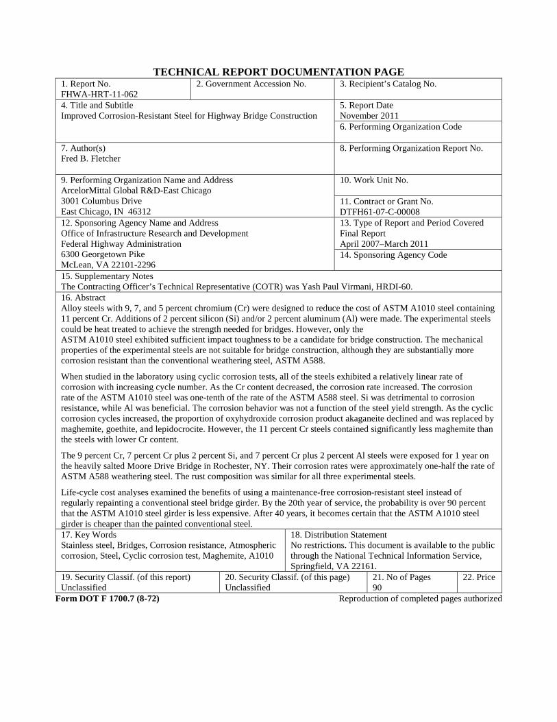
TECHNICAL REPORT DOCUMENTATION PAGE 1. Report No. FHWA-HRT-11-062

2. Government Accession No. 3. Recipient’s Catalog No.

4. Title and Subtitle Improved Corrosion-Resistant Steel for Highway Bridge Construction

5. Report Date November 2011 6. Performing Organization Code

7. Author(s) Fred B. Fletcher

8. Performing Organization Report No.

9. Performing Organization Name and Address ArcelorMittal Global R&D-East Chicago 3001 Columbus Drive East Chicago, IN 46312

10. Work Unit No. 11. Contract or Grant No. DTFH61-07-C-00008

12. Sponsoring Agency Name and Address Office of Infrastructure Research and Development Federal Highway Administration 6300 Georgetown Pike McLean, VA 22101-2296

13. Type of Report and Period Covered Final Report April 2007–March 2011 14. Sponsoring Agency Code

15. Supplementary Notes The Contracting Officer’s Technical Representative (COTR) was Yash Paul Virmani, HRDI-60. 16. Abstract Alloy steels with 9, 7, and 5 percent chromium (Cr) were designed to reduce the cost of ASTM A1010 steel containing 11 percent Cr. Additions of 2 percent silicon (Si) and/or 2 percent aluminum (Al) were made. The experimental steels could be heat treated to achieve the strength needed for bridges. However, only the ASTM A1010 steel exhibited sufficient impact toughness to be a candidate for bridge construction. The mechanical properties of the experimental steels are not suitable for bridge construction, although they are substantially more corrosion resistant than the conventional weathering steel, ASTM A588.

When studied in the laboratory using cyclic corrosion tests, all of the steels exhibited a relatively linear rate of corrosion with increasing cycle number. As the Cr content decreased, the corrosion rate increased. The corrosion rate of the ASTM A1010 steel was one-tenth of the rate of the ASTM A588 steel. Si was detrimental to corrosion resistance, while Al was beneficial. The corrosion behavior was not a function of the steel yield strength. As the cyclic corrosion cycles increased, the proportion of oxyhydroxide corrosion product akaganeite declined and was replaced by maghemite, goethite, and lepidocrocite. However, the 11 percent Cr steels contained significantly less maghemite than the steels with lower Cr content.

The 9 percent Cr, 7 percent Cr plus 2 percent Si, and 7 percent Cr plus 2 percent Al steels were exposed for 1 year on the heavily salted Moore Drive Bridge in Rochester, NY. Their corrosion rates were approximately one-half the rate of ASTM A588 weathering steel. The rust composition was similar for all three experimental steels.

Life-cycle cost analyses examined the benefits of using a maintenance-free corrosion-resistant steel instead of regularly repainting a conventional steel bridge girder. By the 20th year of service, the probability is over 90 percent that the ASTM A1010 steel girder is less expensive. After 40 years, it becomes certain that the ASTM A1010 steel girder is cheaper than the painted conventional steel. 17. Key Words Stainless steel, Bridges, Corrosion resistance, Atmospheric corrosion, Steel, Cyclic corrosion test, Maghemite, A1010

18. Distribution Statement No restrictions. This document is available to the public through the National Technical Information Service, Springfield, VA 22161.

19. Security Classif. (of this report) Unclassified

20. Security Classif. (of this page) Unclassified

21. No of Pages 90

22. Price

Form DOT F 1700.7 (8-72) Reproduction of completed pages authorized

ii

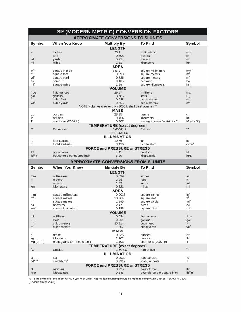
SI* (MODERN METRIC) CONVERSION FACTORS APPROXIMATE CONVERSIONS TO SI UNITS

Symbol When You Know Multiply By To Find Symbol LENGTH

in inches 25.4 millimeters mm ft feet 0.305 meters m yd yards 0.914 meters m mi miles 1.61 kilometers km

AREA in2 square inches 645.2 square millimeters mm2

ft2 square feet 0.093 square meters m2

yd2 square yard 0.836 square meters m2

ac acres 0.405 hectares ha mi2 square miles 2.59 square kilometers km2

VOLUME fl oz fluid ounces 29.57 milliliters mL gal gallons 3.785 liters L ft3 cubic feet 0.028 cubic meters m3

yd3 cubic yards 0.765 cubic meters m3

NOTE: volumes greater than 1000 L shall be shown in m3

MASS oz ounces 28.35 grams glb pounds 0.454 kilograms kgT short tons (2000 lb) 0.907 megagrams (or "metric ton") Mg (or "t")

TEMPERATURE (exact degrees) oF Fahrenheit 5 (F-32)/9 Celsius oC

or (F-32)/1.8 ILLUMINATION

fc foot-candles 10.76 lux lx fl foot-Lamberts 3.426 candela/m2 cd/m2

FORCE and PRESSURE or STRESS lbf poundforce 4.45 newtons N lbf/in2 poundforce per square inch 6.89 kilopascals kPa

APPROXIMATE CONVERSIONS FROM SI UNITS Symbol When You Know Multiply By To Find Symbol

LENGTHmm millimeters 0.039 inches in m meters 3.28 feet ft m meters 1.09 yards yd km kilometers 0.621 miles mi

AREA mm2 square millimeters 0.0016 square inches in2

m2 square meters 10.764 square feet ft2

m2 square meters 1.195 square yards yd2

ha hectares 2.47 acres ac km2 square kilometers 0.386 square miles mi2

VOLUME mL milliliters 0.034 fluid ounces fl oz L liters 0.264 gallons gal m3 cubic meters 35.314 cubic feet ft3

m3 cubic meters 1.307 cubic yards yd3

MASS g grams 0.035 ounces ozkg kilograms 2.202 pounds lbMg (or "t") megagrams (or "metric ton") 1.103 short tons (2000 lb) T

TEMPERATURE (exact degrees) oC Celsius 1.8C+32 Fahrenheit oF

ILLUMINATION lx lux 0.0929 foot-candles fc cd/m2 candela/m2 0.2919 foot-Lamberts fl

FORCE and PRESSURE or STRESS N newtons 0.225 poundforce lbf kPa kilopascals 0.145 poundforce per square inch lbf/in2

*SI is the symbol for th International System of Units. Appropriate rounding should be made to comply with Section 4 of ASTM E380. e(Revised March 2003)

iii

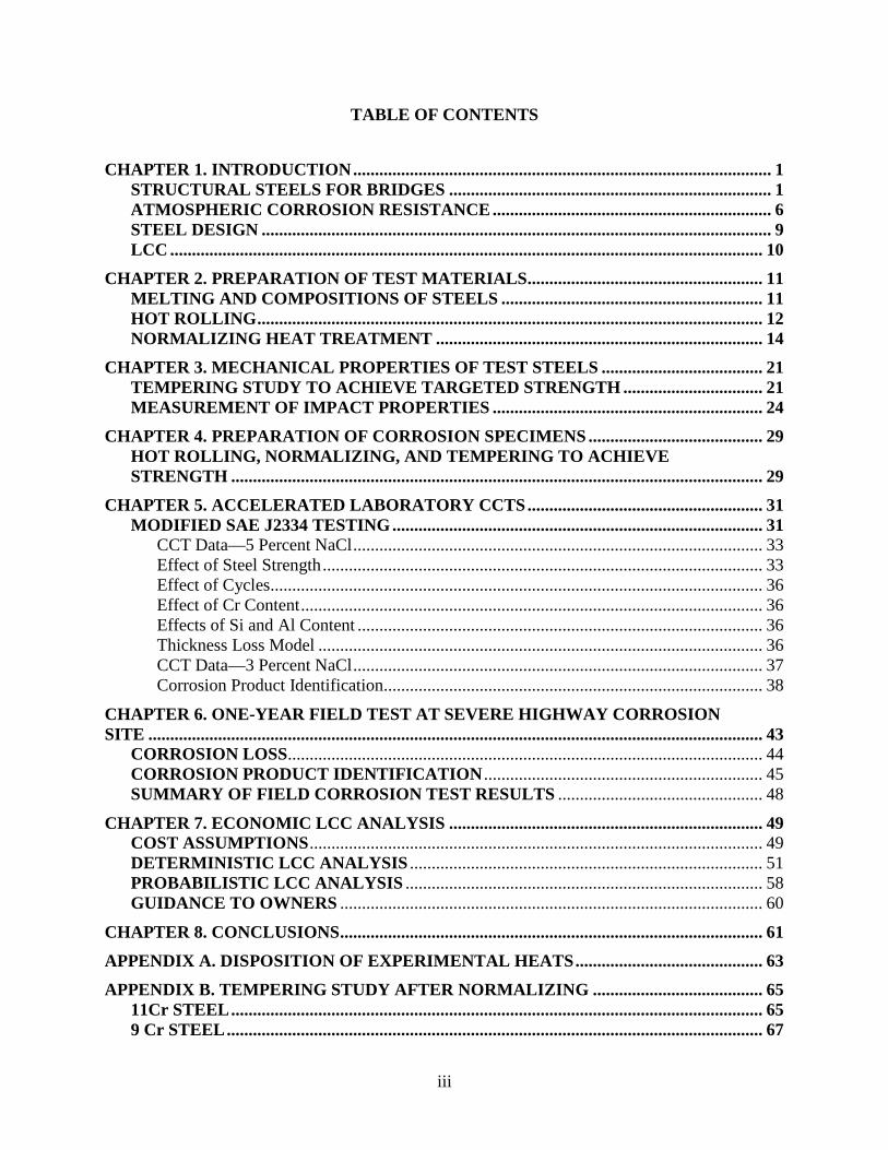
TABLE OF CONTENTS

CHAPTER 1. INTRODUCTION ................................................................................................ 1 STRUCTURAL STEELS FOR BRIDGES .......................................................................... 1 ATMOSPHERIC CORROSION RESISTANCE ................................................................ 6 STEEL DESIGN ..................................................................................................................... 9 LCC ........................................................................................................................................ 10

CHAPTER 2. PREPARATION OF TEST MATERIALS ...................................................... 11 MELTING AND COMPOSITIONS OF STEELS ............................................................ 11 HOT ROLLING .................................................................................................................... 12 NORMALIZING HEAT TREATMENT ........................................................................... 14

CHAPTER 3. MECHANICAL PROPERTIES OF TEST STEELS ..................................... 21 TEMPERING STUDY TO ACHIEVE TARGETED STRENGTH ................................ 21 MEASUREMENT OF IMPACT PROPERTIES .............................................................. 24

CHAPTER 4. PREPARATION OF CORROSION SPECIMENS ........................................ 29 HOT ROLLING, NORMALIZING, AND TEMPERING TO ACHIEVE STRENGTH .......................................................................................................................... 29

CHAPTER 5. ACCELERATED LABORATORY CCTS ...................................................... 31 MODIFIED SAE J2334 TESTING ..................................................................................... 31

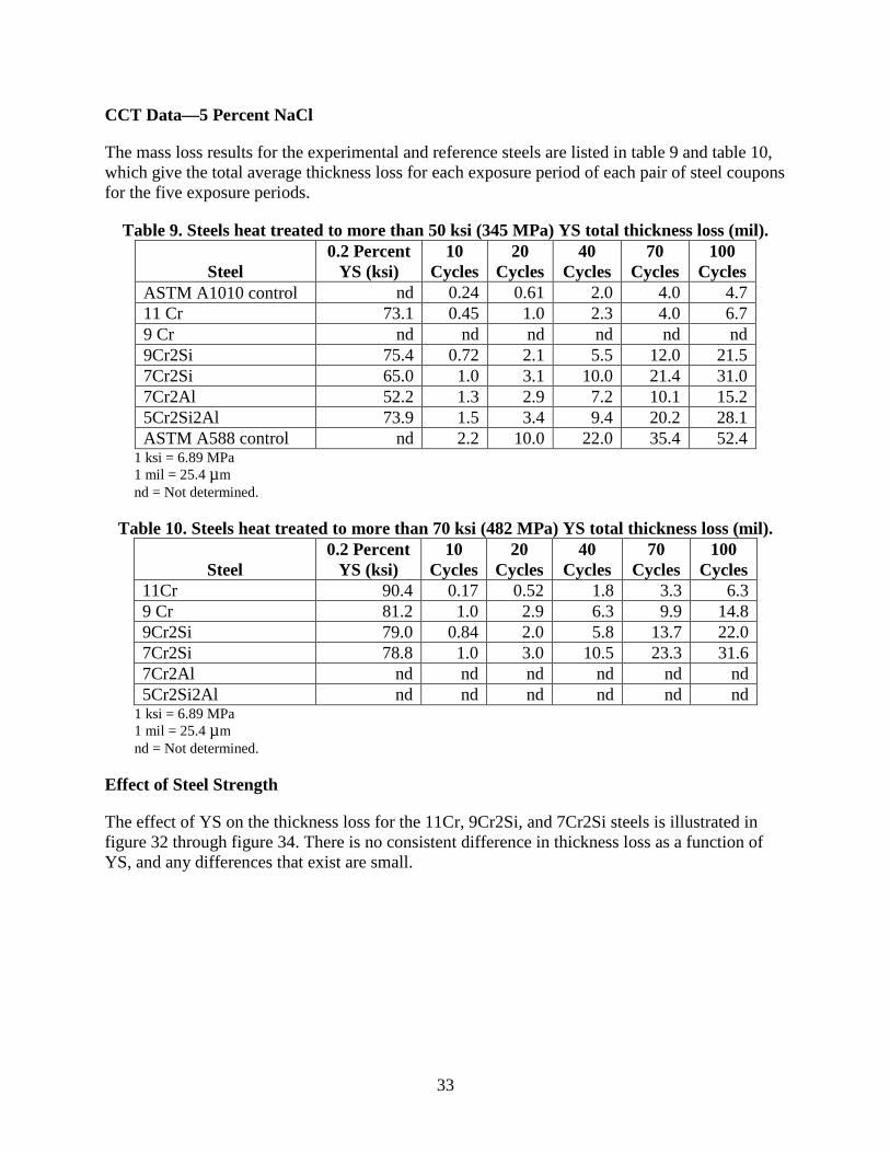
CCT Data—5 Percent NaCl .............................................................................................. 33 Effect of Steel Strength ..................................................................................................... 33 Effect of Cycles................................................................................................................. 36 Effect of Cr Content .......................................................................................................... 36 Effects of Si and Al Content ............................................................................................. 36 Thickness Loss Model ...................................................................................................... 36 CCT Data—3 Percent NaCl .............................................................................................. 37 Corrosion Product Identification ....................................................................................... 38

CHAPTER 6. ONE-YEAR FIELD TEST AT SEVERE HIGHWAY CORROSION SITE ............................................................................................................................................. 43

CORROSION LOSS ............................................................................................................. 44 CORROSION PRODUCT IDENTIFICATION ................................................................ 45 SUMMARY OF FIELD CORROSION TEST RESULTS ............................................... 48

CHAPTER 7. ECONOMIC LCC ANALYSIS ........................................................................ 49 COST ASSUMPTIONS ........................................................................................................ 49 DETERMINISTIC LCC ANALYSIS ................................................................................. 51 PROBABILISTIC LCC ANALYSIS .................................................................................. 58 GUIDANCE TO OWNERS ................................................................................................. 60

CHAPTER 8. CONCLUSIONS ................................................................................................. 61

APPENDIX A. DISPOSITION OF EXPERIMENTAL HEATS ........................................... 63

APPENDIX B. TEMPERING STUDY AFTER NORMALIZING ....................................... 65 11Cr STEEL .......................................................................................................................... 65 9 Cr STEEL ........................................................................................................................... 67

iv

9Cr2Si STEEL ....................................................................................................................... 68 7Cr2Si STEEL ....................................................................................................................... 69 7Cr2Al STEEL ...................................................................................................................... 70 5Cr2Si2Al STEEL ................................................................................................................. 71

APPENDIX C. CORROSION PRODUCTS ON CCT COUPONS ....................................... 73

REFERENCES ............................................................................................................................ 79

v

LIST OF FIGURES

Figure 1. Photo. Fairview Road Bridge over the Glen-Colusa Canal in Colusa, CA ..................... 2 Figure 2. Illustration. Stress strain curve of tensile test .................................................................. 3 Figure 3. Illustration. Round tensile specimen before tensile test .................................................. 3 Figure 4. Illustration. Charpy impact test machine and broken specimen ...................................... 5 Figure 5. Graph. Effect of tempering temperature on YS and Charpy impact toughness of ASTM A1010 steel ......................................................................................................................... 6 Figure 6. Graph. 4-year thickness loss at the 82-ft (25-m) lot in Kure Beach, NC ........................ 7 Figure 7. Graph. 4-year thickness loss at the 656-ft (200-m) lot in Kure Beach, NC .................... 7 Figure 8. Photo. Heat 67-V1-83 being hot rolled prior to first pass ............................................. 12 Figure 9. Photo. Heat 67-V1-83 being hot rolled after last pass................................................... 13 Figure 10. Photo. Heat 67-V1-79 being hot rolled and showing scab .......................................... 13 Figure 11. Photo. Heat 67-V1-79 after hot rolling and showing scab .......................................... 14 Figure 12. Photo. Microstructure of 11Cr plate from heat 67-V1-77 in the as-normalized condition: 100X ............................................................................................................................ 15 Figure 13. Photo. Microstructure of 11Cr plate from heat 67-V1-77 in the as-normalized condition: 500X ............................................................................................................................ 15 Figure 14. Photo. Microstructure of 9Cr plate from heat 67-V1-68 in the as-normalized condition: 100X ............................................................................................................................ 15 Figure 15. Photo. Microstructure of 9Cr plate from heat 67-V1-68 in the as-normalized condition: 500X ............................................................................................................................ 16 Figure 16. Photo. Microstructure of 9Cr2Si plate from heat 67-V1-71 in the as-normalized condition: 100X ............................................................................................................................ 16 Figure 17. Photo. Microstructure of 9Cr2Si plate from heat 67-V1-71 in the as-normalized condition: 500X ............................................................................................................................ 16 Figure 18. Photo. Microstructure of 7Cr2Si plate from heat 67-V1-73 in the as-normalized condition: 100X ............................................................................................................................ 17 Figure 19. Photo. Microstructure of 7Cr2Si plate from heat 67-V1-73 in the as-normalized condition: 500X ............................................................................................................................ 17 Figure 20. Photo. Microstructure of 7Cr2Al plate from heat 67-V1-75 in the as-normalized condition: 50X .............................................................................................................................. 18 Figure 21. Photo. Microstructure of 7Cr2Al plate from heat 67-V1-75 in the as-normalized condition: 500X ............................................................................................................................ 18 Figure 22. Photo. Microstructure of 5Cr2Si2Al plate from heat 67-V1-80 in the as-normalized condition: 50X .............................................................................................................................. 18 Figure 23. Photo. Microstructure of 5Cr2Si2Al plate from heat 67-V1-80 in the as-normalized condition: 500X ............................................................................................................................ 19 Figure 24. Graph. Hardness of as-normalized experimental steels .............................................. 20 Figure 25. Graph. Hardness of the experimental steels after tempering ....................................... 22 Figure 26. Graph. YS of experimental steels after normalizing and tempering ........................... 23 Figure 27. Graph. TS of experimental steels after normalizing and tempering ............................ 24 Figure 28. Graph. Average CVN absorbed energy values for experimental steels tempered to achieve YS greater than 50 ksi (345 MPa) ................................................................................... 26 Figure 29. Graph. Average CVN absorbed energy values for experimental steels tempered to achieve YS greater than 70 ksi (482 MPa) ................................................................................... 26

vi

Figure 30. Photo. Cyclic corrosion chamber ................................................................................ 31 Figure 31. Photo. Interior of cyclic corrosion chamber showing corrosion test panels ................ 32 Figure 32. Graph. Thickness loss at two different strength levels for 11Cr steel ......................... 34 Figure 33. Graph. Thickness loss at two different strength levels for 9Cr2Si steel ..................... 34 Figure 34. Graph. Thickness loss at two different strength levels for 7Cr2Si steel ..................... 34 Figure 35. Graph. Summary of 5 percent NaCl CCT results ........................................................ 35 Figure 36. Photo. Corrosion coupons on Moore Drive Bridge on rack 1 just prior to removal after 1-year exposure ...................................................................................................... 44 Figure 37. Illustration. Example bridge girder 80 ft (24.4 m) long .............................................. 51 Figure 38. Graph. Change of the total cost with time assuming a repainting interval of 20 years and a discount rate of 0 percent ...................................................................................... 53 Figure 39. Graph. Change of the total cost with time assuming a repainting interval of 15 years and a discount rate of 0 percent ...................................................................................... 54 Figure 40. Graph. Change of the total cost with time assuming a repainting interval of 10 years and a discount rate of 0 percent ...................................................................................... 55 Figure 41. Graph. Change of the total cost with time assuming a repainting interval of 20 years and a discount rate of 3 percent ...................................................................................... 56 Figure 42. Graph. Change of total cost with time assuming a repainting every 15 years and a discount rate of 3 percent .................................................................................................... 57 Figure 43. Graph. Change of the total cost with time assuming a repainting interval of 10 years and a discount rate of 3 percent ...................................................................................... 58 Figure 44. Graph. Change of the mean total cost with time for the conventional painted carbon steel girder and the unpainted ASTM A1010 steel girder ................................................ 59 Figure 45. Graph. Probability that Cconv is higher than CA1010 with time ...................................... 60 Figure 46. Graph. Tensile properties of normalized and tempered 11Cr steel ............................. 66 Figure 47. Graph. Tensile properties of normalized and tempered 9Cr steel ............................... 67 Figure 48. Graph. Tensile properties of normalized and tempered 9Cr2Si steel .......................... 68 Figure 49. Graph. Tensile properties of normalized and tempered 7Cr2Si steel .......................... 69 Figure 50. Graph. Tensile properties of normalized and tempered 7Cr2Al steel ......................... 70 Figure 51. Graph. Tensile properties of normalized and tempered 5Cr2Si2Al steel .................... 71

vii

LIST OF TABLES

Table 1. Mechanical properties of ASTM A1010 production plates and specified minimum properties for ASTM A709-50W and A709-70W in nonfracture critical (NFC) bridge design elements ........................................................................................................ 4 Table 2. Target compositions of experimental steels.................................................................... 10 Table 3. Composition of experimental 100-lb (45-kg) heats ........................................................ 11 Table 4. As-normalized hardness and microstructure................................................................... 19 Table 5. Hardness of experimental steels as a function of tempering temperature ...................... 21 Table 6. Tensile properties of as-normalized steel plates ............................................................. 23 Table 7. Tempering temperatures for CVN impact energy and corrosion studies ....................... 25 Table 8. CVN impact test results (ft-lb)........................................................................................ 25 Table 9. Steels heat treated to more than 50 ksi (345 MPa) YS total thickness loss (mil) ........... 33 Table 10. Steels heat treated to more than 70 ksi (482 MPa) YS total thickness loss (mil) ......... 33 Table 11. CCT results using 5 percent NaCl total thickness loss (mil) ........................................ 35 Table 12. Linear regression equations for thickness loss in 5 percent NaCl CCTs ...................... 37 Table 13. CCT results using 3 percent NaCl total thickness loss (mil) ........................................ 37 Table 14. Linear regression equations for thickness loss CCTs ................................................... 38 Table 15. Corrosion products on coupons sprayed with 5 percent NaCl (percent) ...................... 40 Table 16. Overall average corrosion products from 5 percent NaCl CCTs (percent) .................. 41 Table 17. Thickness loss of experimental steels exposed and historical data for control steels exposed on Moore Drive Bridge ................................................................................................... 45 Table 18. Composition of the rusts on the upward-facing surface of the three experimental steels exposed on Moore Drive Bridge (percent) ......................................................................... 46 Table 19. Chloride concentrations measured in the rust formed on Moore Drive Bridge (percent) ........................................................................................................................................ 47 Table 20. Total model girder initial costs ..................................................................................... 52 Table 21. Disposition of experimental heats................................................................................. 63 Table 22. Tensile test results of 11Cr and ASTM A1010 steels ................................................... 65 Table 23. Tensile test results of 9Cr steel ..................................................................................... 67 Table 24. Tensile test results of 9Cr2Si steel ................................................................................ 68 Table 25. Tensile test results of 7Cr2Si steel ................................................................................ 69 Table 26. Tensile test results of 7Cr2Al steel ............................................................................... 70 Table 27. Tensile test results of 5Cr2Si2Al steel .......................................................................... 71 Table 28. Rust percentage after 10 cycles of 5 percent NaCl ....................................................... 74 Table 29. Rust percentage after 20 cycles of 5 percent NaCl ....................................................... 75 Table 30. Rust percentage after 40 cycles of 5 percent NaCl ...................................................... 76 Table 31. Rust percentage after 70 cycles of 5 percent NaCl ...................................................... 77 Table 32. Rust percentage after 100 cycles in 5 percent NaCl ..................................................... 78

viii

ABBREVIATIONS AND SYMBOLS

Abbreviations CCT Cyclic corrosion test

CI Corrosion index

CVN Charpy V-notch

DA Rust from downward-facing coupon surface

DAU Rust from under the course rust from the downward-facing surface

DT Rust from the top part of the downward-facing surface

FC Fracture critical

EL Tensile elongation

EUL YS Elongation under load yield strength

HBW Brinell Hardness number

ksi 1,000 psi

kV kilovolts

LCC Life-cycle cost

LCVN Longitudinal Charpy V-notch

mA milliamperes

mil One-thousandth of an inch

mpy mil per year

NFC Nonfracture critical

RA Reduction of area

sa Semi-adherent rust

SAE Society of Automotive Engineers

TS Tensile strength

UA Rust from upward-facing coupon surface

UAF Fine rust from all upward-facing surfaces

UAU Rust from under the course rust from the upward-facing surface

UB Rust from bottom part of the upward-facing surface

UT Rust from top part of the upward-facing surface

USGS United States Geological Survey

va Very adherent rust

XRD X-ray diffraction

ix

XRF X-ray fluorescence

YS Yield strength

Symbols α Greek letter alpha α -FeOOH Goethite

Al Aluminum β Greek letter beta β -FeOOH Akaganeite

γ Greek letter gamma

γ -FeOOH Lepidocrocite

C Carbon

CA1010 Cost of the ASTM A1010 steel girder

Cconv Cost of the conventional painted steel girder

Cr Chromium

Cu Copper

FeO·Fe2O3 Maghemite

h0 Original height of Charpy hammer

h Final height of Charpy hammer after impacting test specimen

Mn Manganese

Mo Molybdenum

N Nitrogen

n-value Strain hardening coefficient in a tensile test

NaCl Sodium chloride

Ni Nickel

P Phosphorus R2 Coefficient of determination

S Sulfur

Si Silicon

t Paint application time

V Vanadium ν Discount rate of money

1

CHAPTER 1. INTRODUCTION

Highway bridges must perform safely and economically for many years during adverse environmental conditions. Steel highway bridge structural elements can corrode, which decreases thickness and increases stresses in load-carrying members. As a result, highway bridges must be designed to mitigate the long-term effects of corrosion. Mitigation approaches include painting and using weathering steel grades and high-performance weathering steels such as those described in ASTM A709.(2) Painting and other surface treatments must be maintained over the projected life of the bridge. The costs associated with maintenance represent a significant burden on the bridge owner, and the life-cycle cost (LCC) of a painted bridge can be significantly higher than a maintenance-free weathering steel bridge.

STRUCTURAL STEELS FOR BRIDGES

Weathering steels do not require maintenance for corrosion protection in most environments. However, the corrosion rate of weathering steels may be unsatisfactory in severe service conditions where the protective patina does not form on the steel surfaces. In such adverse environments, conventional weathering steels do not provide sufficient corrosion resistance.

An economical stainless steel described in ASTM A1010 represents an engineering material that meets the strength and impact toughness requirements of the most commonly used ASTM A709 bridge steels.(1,2) ASTM A1010 steel overcomes the corrosion limitations of conventional weathering grades, but with a first-cost economic penalty. The LCC analysis of ASTM A1010 in a 100-year-old bridge may prove the steel to be the lowest cost material of construction. Any measure that can lower the initial cost of this steel will improve its LCC.

Conventional and high-performance weathering steels described in ASTM A709 perform well except in protracted time-of-wetness conditions and when chlorides are deposited on the steel either naturally (i.e., in coastal locations) or in snow belt regions where deicing salts are heavily applied.(2,3) The reason for this behavior is related to the development—or lack of development—of a protective oxide or oxy-hydroxide layer on the weathering steel surface.(4) Development of such a layer on weathering steel requires frequent drying that allows nanophase goethite (α -FeOOH) to form in the absence of moisture. It is the nanophase goethite that constitutes the primary impenetrable layer on weathering steel.(5) When a certain, and as yet unknown, level of chlorides is present in the oxy-hydroxide surface layer, formation of nanophase goethite is inhibited, and akaganeite (β -FeOOH) and/or maghemite (FeO·Fe2O3) formation are favored. This is the reason coastal and deicing salt environments are unsatisfactory for weathering steels.

The structural steel ASTM A1010 has been shown to exhibit very low corrosion losses compared to weathering steels through accelerated laboratory tests and coastal exposures.(6) ASTM A1010 is defined as a stainless steel because its chromium (Cr) content is nominally 12 percent Cr, which is well above the 10.5 percent Cr that defines the lower limit of Cr for stainless steel. Stainless steel has a different mechanism for corrosion protection than weathering steels. Instead of nanophase goethite that forms on weathering steel, Cr oxide forms on stainless steel as a thin continuous film on the surface.

2

One approach used to reduce the cost of ASTM A1010 steel for highway bridge application is to lower its Cr content while maintaining satisfactory strength and impact toughness. However, such a change may significantly reduce the atmospheric corrosion resistance where high time-of-wetness and/or elevated chloride contents are present. The current study was designed to explore this possibility and to achieve the Federal Highway Administration’s objective to identify an economical steel grade suitable for use in severe highway bridge environments that does not require a supplemental protective coating.

ASTM A1010 steel has been in production in the United States since 1992 and elsewhere in the world since the 1970s. Currently, over 25,000 T (227 million kg) of this steel has been produced in the United States in at least four different steel melt shops. Additionally, there is an established domestic production capability for a new steel based on ASTM A1010.(1)

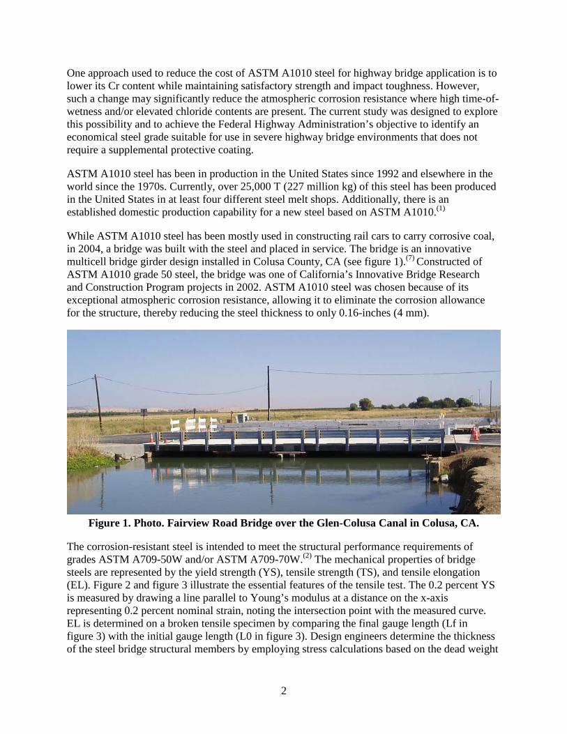
While ASTM A1010 steel has been mostly used in constructing rail cars to carry corrosive coal, in 2004, a bridge was built with the steel and placed in service. The bridge is an innovative multicell bridge girder design installed in Colusa County, CA (see figure 1).(7) Constructed of ASTM A1010 grade 50 steel, the bridge was one of California’s Innovative Bridge Research and Construction Program projects in 2002. ASTM A1010 steel was chosen because of its exceptional atmospheric corrosion resistance, allowing it to eliminate the corrosion allowance for the structure, thereby reducing the steel thickness to only 0.16-inches (4 mm).

Figure 1. Photo. Fairview Road Bridge over the Glen-Colusa Canal in Colusa, CA.

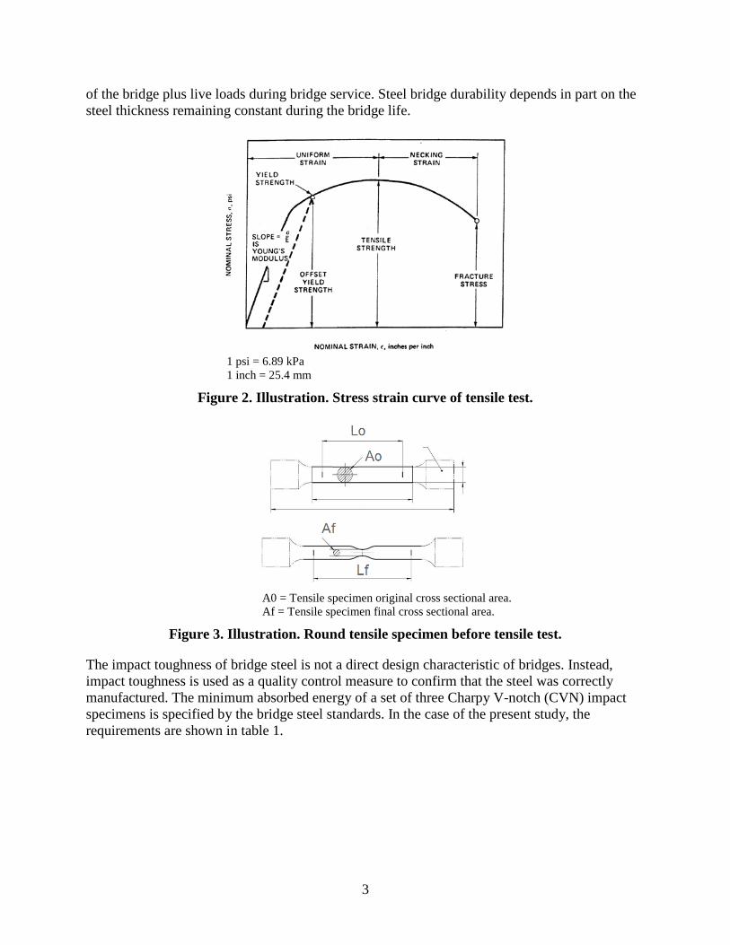
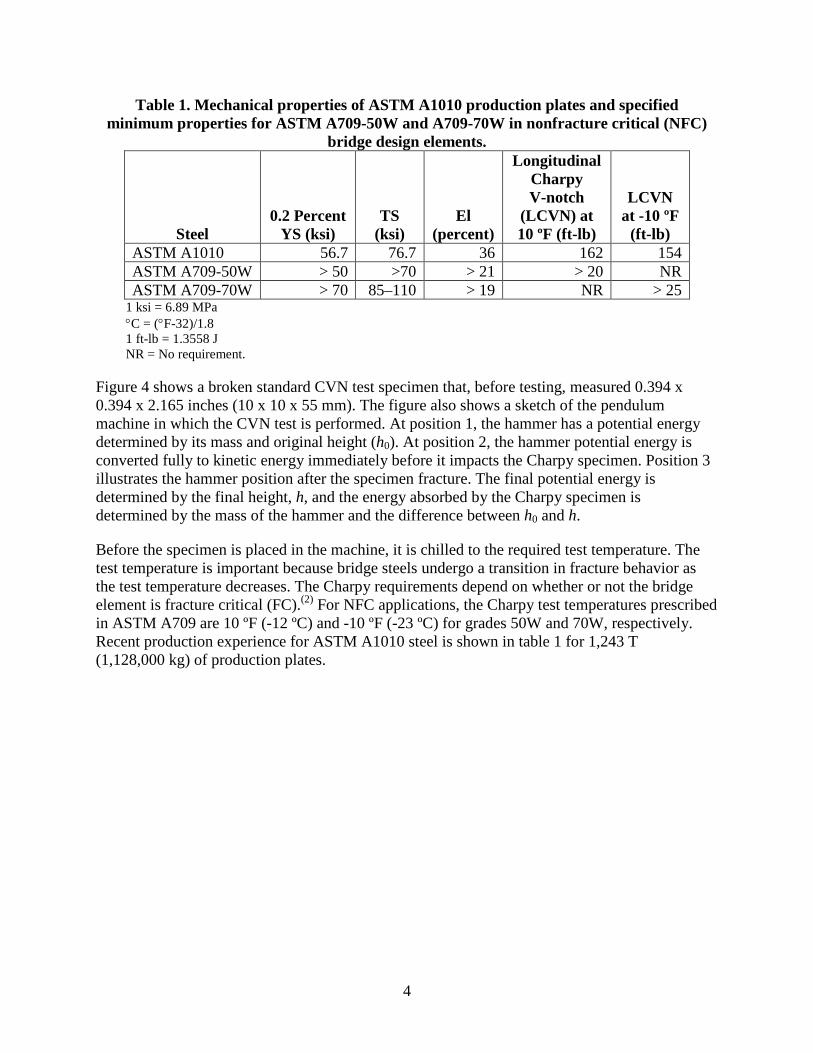
The corrosion-resistant steel is intended to meet the structural performance requirements of grades ASTM A709-50W and/or ASTM A709-70W.(2) The mechanical properties of bridge steels are represented by the yield strength (YS), tensile strength (TS), and tensile elongation (EL). Figure 2 and figure 3 illustrate the essential features of the tensile test. The 0.2 percent YS is measured by drawing a line parallel to Young’s modulus at a distance on the x-axis representing 0.2 percent nominal strain, noting the intersection point with the measured curve. EL is determined on a broken tensile specimen by comparing the final gauge length (Lf in figure 3) with the initial gauge length (L0 in figure 3). Design engineers determine the thickness of the steel bridge structural members by employing stress calculations based on the dead weight

3

of the bridge plus live loads during bridge service. Steel bridge durability depends in part on the steel thickness remaining constant during the bridge life.

1 psi = 6.89 kPa 1 inch = 25.4 mm

Figure 2. Illustration. Stress strain curve of tensile test.

A0 = Tensile specimen original cross sectional area. Af = Tensile specimen final cross sectional area.

Figure 3. Illustration. Round tensile specimen before tensile test.

The impact toughness of bridge steel is not a direct design characteristic of bridges. Instead, impact toughness is used as a quality control measure to confirm that the steel was correctly manufactured. The minimum absorbed energy of a set of three Charpy V-notch (CVN) impact specimens is specified by the bridge steel standards. In the case of the present study, the requirements are shown in table 1.

4

Table 1. Mechanical properties of ASTM A1010 production plates and specified minimum properties for ASTM A709-50W and A709-70W in nonfracture critical (NFC)

bridge design elements.

Steel 0.2 Percent

YS (ksi) TS

(ksi) El

(percent)

Longitudinal Charpy V-notch

(LCVN) at 10 ºF (ft-lb)

LCVN at -10 ºF

(ft-lb) ASTM A1010

56.7 76.7 36 162 154

ASTM A709-50W > 50 >70 > 21 > 20 NR ASTM A709-70W > 70 85–110 > 19 NR > 25

1 ksi = 6.89 MPa °C = (°F-32)/1.8 1 ft-lb = 1.3558 J NR = No requirement.

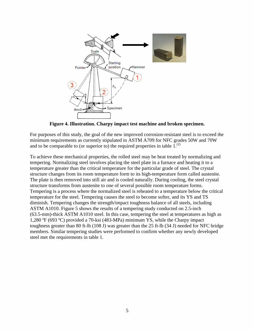
Figure 4 shows a broken standard CVN test specimen that, before testing, measured 0.394 x 0.394 x 2.165 inches (10 x 10 x 55 mm). The figure also shows a sketch of the pendulum machine in which the CVN test is performed. At position 1, the hammer has a potential energy determined by its mass and original height (h0). At position 2, the hammer potential energy is converted fully to kinetic energy immediately before it impacts the Charpy specimen. Position 3 illustrates the hammer position after the specimen fracture. The final potential energy is determined by the final height, h, and the energy absorbed by the Charpy specimen is determined by the mass of the hammer and the difference between h0 and h.

Before the specimen is placed in the machine, it is chilled to the required test temperature. The test temperature is important because bridge steels undergo a transition in fracture behavior as the test temperature decreases. The Charpy requirements depend on whether or not the bridge element is fracture critical (FC).(2) For NFC applications, the Charpy test temperatures prescribed in ASTM A709 are 10 ºF (-12 ºC) and -10 ºF (-23 ºC) for grades 50W and 70W, respectively. Recent production experience for ASTM A1010 steel is shown in table 1 for 1,243 T (1,128,000 kg) of production plates.

5

Figure 4. Illustration. Charpy impact test machine and broken specimen.

For purposes of this study, the goal of the new improved corrosion-resistant steel is to exceed the minimum requirements as currently stipulated in ASTM A709 for NFC grades 50W and 70W and to be comparable to (or superior to) the required properties in table 1.(2)

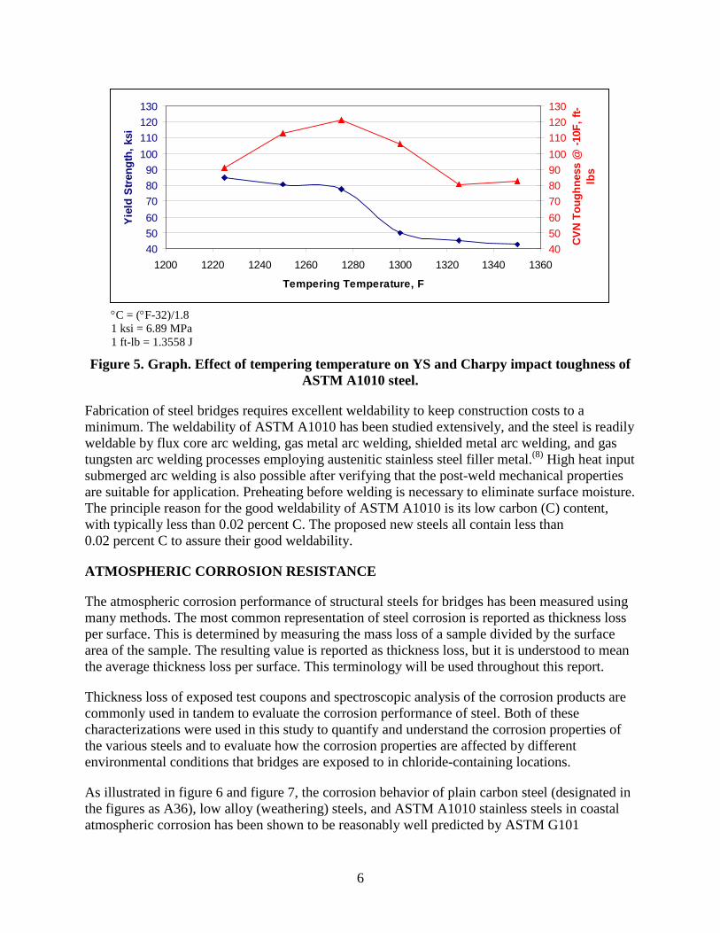
To achieve these mechanical properties, the rolled steel may be heat treated by normalizing and tempering. Normalizing steel involves placing the steel plate in a furnace and heating it to a temperature greater than the critical temperature for the particular grade of steel. The crystal structure changes from its room temperature form to its high-temperature form called austenite. The plate is then removed into still air and is cooled naturally. During cooling, the steel crystal structure transforms from austenite to one of several possible room temperature forms. Tempering is a process where the normalized steel is reheated to a temperature below the critical temperature for the steel. Tempering causes the steel to become softer, and its YS and TS diminish. Tempering changes the strength/impact toughness balance of all steels, including ASTM A1010. Figure 5 shows the results of a tempering study conducted on 2.5-inch (63.5-mm)-thick ASTM A1010 steel. In this case, tempering the steel at temperatures as high as 1,280 ºF (693 ºC) provided a 70-ksi (483-MPa) minimum YS, while the Charpy impact toughness greater than 80 ft-lb (108 J) was greater than the 25 ft-lb (34 J) needed for NFC bridge members. Similar tempering studies were performed to confirm whether any newly developed steel met the requirements in table 1.

6

405060708090

100110120130

1200 1220 1240 1260 1280 1300 1320 1340 1360

Tempering Temperature, F

Yiel

d St

reng

th, k

si

405060708090100110120130

CVN

Toug

hnes

s @

-10F

, ft-

lbs

°C = (°F-32)/1.8 1 ksi = 6.89 MPa 1 ft-lb = 1.3558 J

Figure 5. Graph. Effect of tempering temperature on YS and Charpy impact toughness of ASTM A1010 steel.

Fabrication of steel bridges requires excellent weldability to keep construction costs to a minimum. The weldability of ASTM A1010 has been studied extensively, and the steel is readily weldable by flux core arc welding, gas metal arc welding, shielded metal arc welding, and gas tungsten arc welding processes employing austenitic stainless steel filler metal.(8) High heat input submerged arc welding is also possible after verifying that the post-weld mechanical properties are suitable for application. Preheating before welding is necessary to eliminate surface moisture. The principle reason for the good weldability of ASTM A1010 is its low carbon (C) content, with typically less than 0.02 percent C. The proposed new steels all contain less than 0.02 percent C to assure their good weldability.

ATMOSPHERIC CORROSION RESISTANCE

The atmospheric corrosion performance of structural steels for bridges has been measured using many methods. The most common representation of steel corrosion is reported as thickness loss per surface. This is determined by measuring the mass loss of a sample divided by the surface area of the sample. The resulting value is reported as thickness loss, but it is understood to mean the average thickness loss per surface. This terminology will be used throughout this report.

Thickness loss of exposed test coupons and spectroscopic analysis of the corrosion products are commonly used in tandem to evaluate the corrosion performance of steel. Both of these characterizations were used in this study to quantify and understand the corrosion properties of the various steels and to evaluate how the corrosion properties are affected by different environmental conditions that bridges are exposed to in chloride-containing locations.

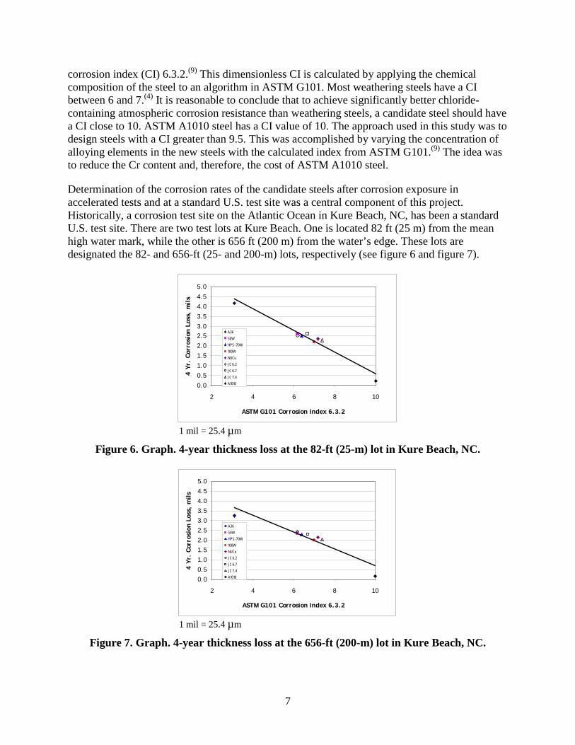
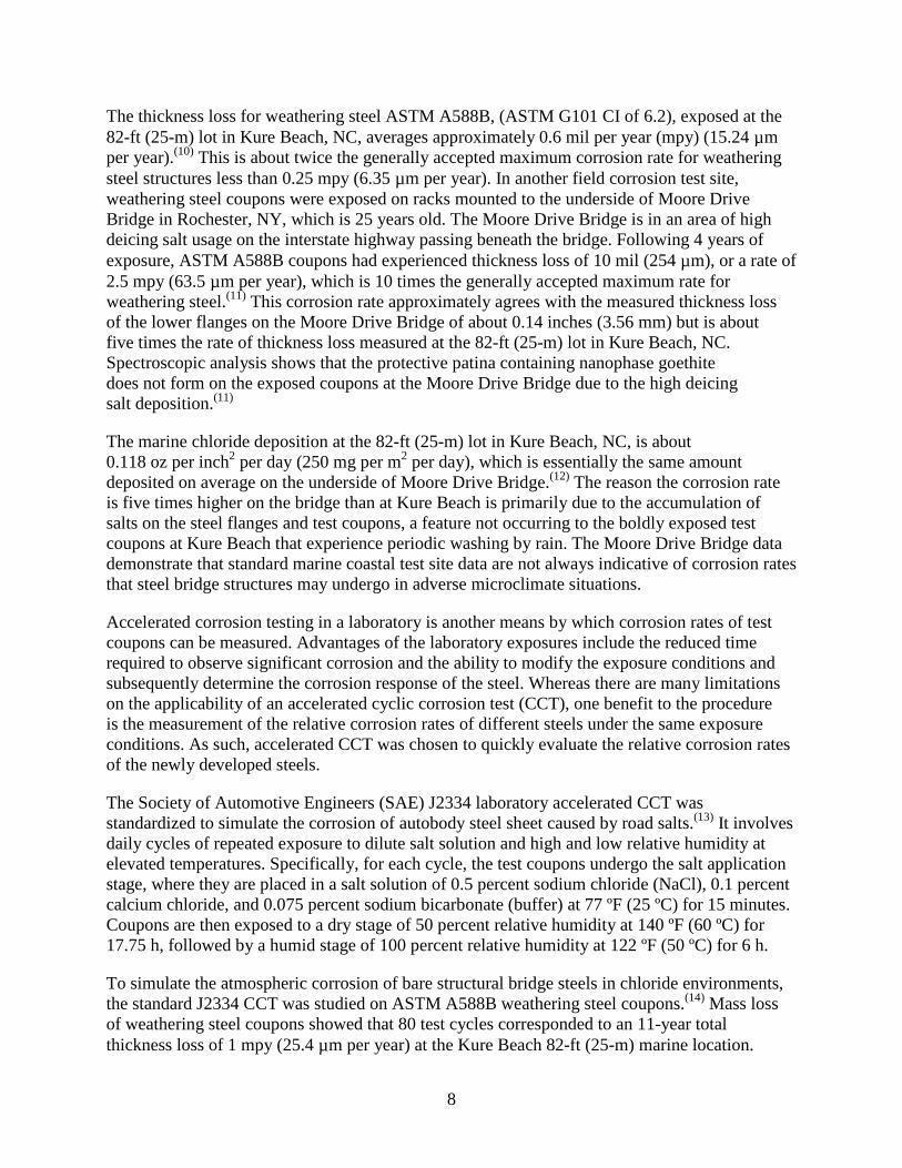
As illustrated in figure 6 and figure 7, the corrosion behavior of plain carbon steel (designated in the figures as A36), low alloy (weathering) steels, and ASTM A1010 stainless steels in coastal atmospheric corrosion has been shown to be reasonably well predicted by ASTM G101

7

corrosion index (CI) 6.3.2.(9) This dimensionless CI is calculated by applying the chemical composition of the steel to an algorithm in ASTM G101. Most weathering steels have a CI between 6 and 7.(4) It is reasonable to conclude that to achieve significantly better chloride-containing atmospheric corrosion resistance than weathering steels, a candidate steel should have a CI close to 10. ASTM A1010 steel has a CI value of 10. The approach used in this study was to design steels with a CI greater than 9.5. This was accomplished by varying the concentration of alloying elements in the new steels with the calculated index from ASTM G101.(9) The idea was to reduce the Cr content and, therefore, the cost of ASTM A1010 steel.

Determination of the corrosion rates of the candidate steels after corrosion exposure in accelerated tests and at a standard U.S. test site was a central component of this project. Historically, a corrosion test site on the Atlantic Ocean in Kure Beach, NC, has been a standard U.S. test site. There are two test lots at Kure Beach. One is located 82 ft (25 m) from the mean high water mark, while the other is 656 ft (200 m) from the water’s edge. These lots are designated the 82- and 656-ft (25- and 200-m) lots, respectively (see figure 6 and figure 7).

0.0

0.5

1.0

1.5

2.0

2.53.0

3.5

4.0

4.5

5.0

2 4 6 8 10

ASTM G101 Corrosion Index 6.3.2

4 Yr

. Co

rros

ion

Loss

, m

ils

A3650WHPS-70W100WNUCuJC 6.2JC 6.7JC 7.4A1010

1 mil = 25.4 µ m

Figure 6. Graph. 4-year thickness loss at the 82-ft (25-m) lot in Kure Beach, NC.

0.0

0.5

1.0

1.5

2.0

2.5

3.0

3.5

4.0

4.5

5.0

2 4 6 8 10

ASTM G101 Corrosion Index 6.3.2

4 Yr

. Co

rros

ion

Loss

, m

ils

A3650WHPS-70W100WNUCuJC 6.2JC 6.7JC 7.4A1010

1 mil = 25.4 µ m

Figure 7. Graph. 4-year thickness loss at the 656-ft (200-m) lot in Kure Beach, NC.

8

The thickness loss for weathering steel ASTM A588B, (ASTM G101 CI of 6.2), exposed at the 82-ft (25-m) lot in Kure Beach, NC, averages approximately 0.6 mil per year (mpy) (15.24 µ m per year).(10) This is about twice the generally accepted maximum corrosion rate for weathering steel structures less than 0.25 mpy (6.35 µ m per year). In another field corrosion test site, weathering steel coupons were exposed on racks mounted to the underside of Moore Drive Bridge in Rochester, NY, which is 25 years old. The Moore Drive Bridge is in an area of high deicing salt usage on the interstate highway passing beneath the bridge. Following 4 years of exposure, ASTM A588B coupons had experienced thickness loss of 10 mil (254 µ m), or a rate of 2.5 mpy (63.5 µ m per year), which is 10 times the generally accepted maximum rate for weathering steel.(11) This corrosion rate approximately agrees with the measured thickness loss of the lower flanges on the Moore Drive Bridge of about 0.14 inches (3.56 mm) but is about five times the rate of thickness loss measured at the 82-ft (25-m) lot in Kure Beach, NC. Spectroscopic analysis shows that the protective patina containing nanophase goethite does not form on the exposed coupons at the Moore Drive Bridge due to the high deicing salt deposition.(11)

The marine chloride deposition at the 82-ft (25-m) lot in Kure Beach, NC, is about 0.118 oz per inch2 per day (250 mg per m2 per day), which is essentially the same amount deposited on average on the underside of Moore Drive Bridge.(12) The reason the corrosion rate is five times higher on the bridge than at Kure Beach is primarily due to the accumulation of salts on the steel flanges and test coupons, a feature not occurring to the boldly exposed test coupons at Kure Beach that experience periodic washing by rain. The Moore Drive Bridge data demonstrate that standard marine coastal test site data are not always indicative of corrosion rates that steel bridge structures may undergo in adverse microclimate situations.

Accelerated corrosion testing in a laboratory is another means by which corrosion rates of test coupons can be measured. Advantages of the laboratory exposures include the reduced time required to observe significant corrosion and the ability to modify the exposure conditions and subsequently determine the corrosion response of the steel. Whereas there are many limitations on the applicability of an accelerated cyclic corrosion test (CCT), one benefit to the procedure is the measurement of the relative corrosion rates of different steels under the same exposure conditions. As such, accelerated CCT was chosen to quickly evaluate the relative corrosion rates of the newly developed steels.

The Society of Automotive Engineers (SAE) J2334 laboratory accelerated CCT was standardized to simulate the corrosion of autobody steel sheet caused by road salts.(13) It involves daily cycles of repeated exposure to dilute salt solution and high and low relative humidity at elevated temperatures. Specifically, for each cycle, the test coupons undergo the salt application stage, where they are placed in a salt solution of 0.5 percent sodium chloride (NaCl), 0.1 percent calcium chloride, and 0.075 percent sodium bicarbonate (buffer) at 77 ºF (25 ºC) for 15 minutes. Coupons are then exposed to a dry stage of 50 percent relative humidity at 140 ºF (60 ºC) for 17.75 h, followed by a humid stage of 100 percent relative humidity at 122 ºF (50 ºC) for 6 h.

To simulate the atmospheric corrosion of bare structural bridge steels in chloride environments, the standard J2334 CCT was studied on ASTM A588B weathering steel coupons.(14) Mass loss of weathering steel coupons showed that 80 test cycles corresponded to an 11-year total thickness loss of 1 mpy (25.4 µ m per year) at the Kure Beach 82-ft (25-m) marine location.

9

However, the chloride levels on the SAE J2334 test coupons were an order of magnitude lower (0.1 weight percent) than measured on the bridges, and the rust composition in the preliminary tests subsequently lacked akaganeite in the bridge rusts. Spectroscopic analysis of the SAE J2334 coupons showed that the rust formed was maghemite, an iron oxy-hydroxide known to form due to high time-of-wetness, which dominates the corrosion in low chloride locations.

Modifications to the original SAE J2334 solution chemistry (the chloride concentration was increased by a factor of 10 to 5 percent NaCl) were made.(14) The modified J2334 CCT was successful in forming akaganeite on the bare weathering steel. The chloride in the rust was measured to be 2 percent, the same as the rust on the Moore Drive Bridge. Therefore, successful simulation of the under-bridge environment in adverse locations of high chloride deposition was achieved with the modified J2334 CCT. As a result of this preliminary research, the use of the modified SAE J2334 CCT shows promise for simulating structural steel exposures in adverse environments containing high chloride concentrations and high time-of-wetness.

One limitation of test site coupon exposure projects is the significant time, typically greater than 5 years, needed to expose the coupons to measure meaningful trends in the mass loss as rust forms. To some extent, this is now circumvented by either x-ray, micro-Raman, or Mössbauer spectroscopy to identify the corrosion products forming in early exposure periods. Such data can quickly determine formation, or lack thereof, of the most effective protective patina (mainly nanophase goethite) on weathering steel, and thereby predict long-term corrosion rates of the test steel. It is important to analyze the corrosion products on exposed steel by suitable spectroscopy.(5)

STEEL DESIGN

The current study was based on the objective of modifying the composition of ASTM A1010 steel to lower its cost of production without significantly reducing its chloride-containing atmospheric corrosion resistance, while achieving the strength and impact toughness required by ASTM A709.

ASTM A1010 steel exhibits a dual-phase microstructure of ferrite plus martensite. To obtain this particular microstructure, the composition of the steel must be carefully balanced. In high-Cr steels, some alloying elements (e.g., nickel (Ni), C, nitrogen (N), manganese (Mn), and copper (Cu)) promote the formation of austenite, while others (e.g., Cr, molybdenum (Mo), vanadium (V), silicon (Si), aluminum (Al), and titanium) promote the formation of ferrite.(15) Modifying ASTM A1010 steel to reduce its manufacturing cost, which was the approach taken in this project, must take into account the changed phase balance between austenite and ferrite so that comparable microstructures, mechanical properties, and weldability can be expected. Simply reducing the Cr content of ASTM A1010 steel unbalances the ferrite-austenite phase mixture. As a result, compensating changes must be made to other alloying elements in the steel. To achieve the 50- and 70-ksi (345- and 482-MPa) targeted YS, the compositions were designed to have either a fully martensitic or a dual phase (martensite plus ferrite) microstructure.

The alloy design selected to reduce the cost of ASTM A1010 steel containing 11 percent Cr was to reduce the Cr content to 9, 7, and 5 percent. To compensate for the concomitant diminished corrosion resistance as estimated by ASTM G101, additions of 2 percent Si, 2 percent Al, or a

10

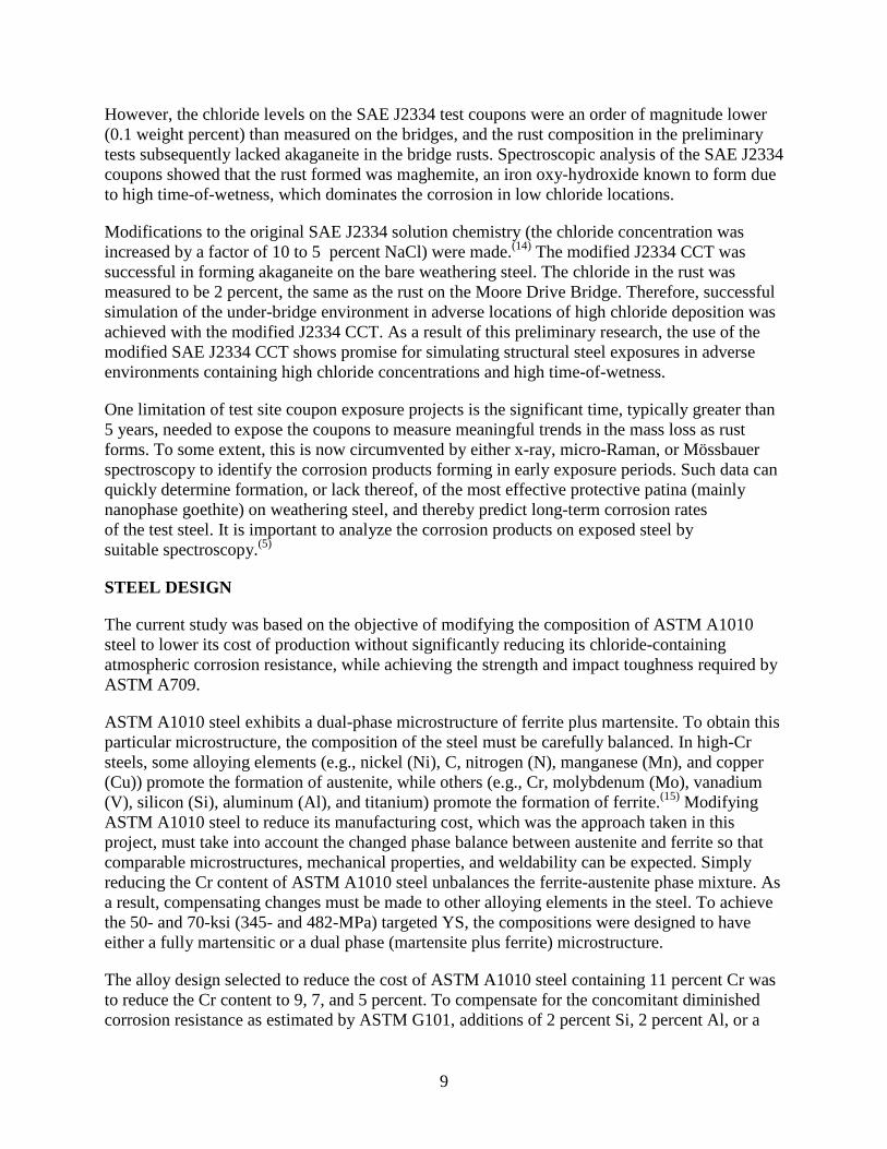
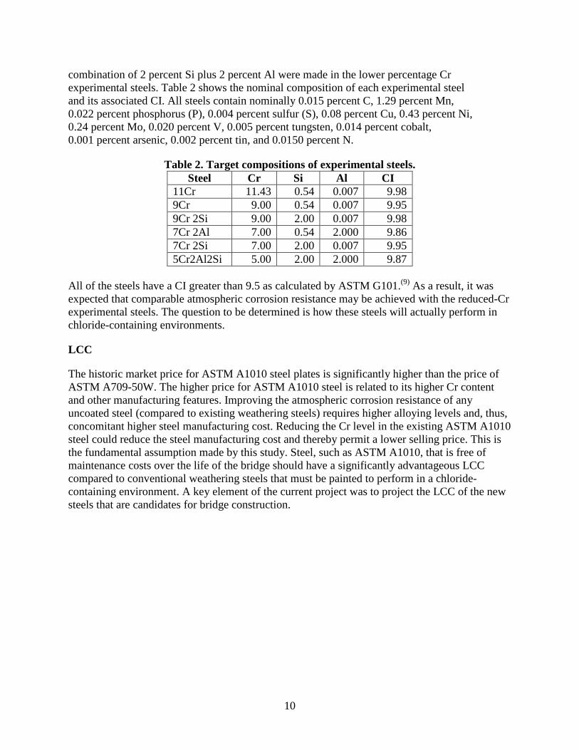
combination of 2 percent Si plus 2 percent Al were made in the lower percentage Cr experimental steels. Table 2 shows the nominal composition of each experimental steel and its associated CI. All steels contain nominally 0.015 percent C, 1.29 percent Mn, 0.022 percent phosphorus (P), 0.004 percent sulfur (S), 0.08 percent Cu, 0.43 percent Ni, 0.24 percent Mo, 0.020 percent V, 0.005 percent tungsten, 0.014 percent cobalt, 0.001 percent arsenic, 0.002 percent tin, and 0.0150 percent N.

Table 2. Target compositions of experimental steels. Steel Cr Si Al CI

11Cr 11.43 0.54 0.007 9.98 9Cr 9.00 0.54 0.007 9.95 9Cr 2Si 9.00 2.00 0.007 9.98 7Cr 2Al 7.00 0.54 2.000 9.86 7Cr 2Si 7.00 2.00 0.007 9.95 5Cr2Al2Si 5.00 2.00 2.000 9.87

All of the steels have a CI greater than 9.5 as calculated by ASTM G101.(9) As a result, it was expected that comparable atmospheric corrosion resistance may be achieved with the reduced-Cr experimental steels. The question to be determined is how these steels will actually perform in chloride-containing environments.

LCC

The historic market price for ASTM A1010 steel plates is significantly higher than the price of ASTM A709-50W. The higher price for ASTM A1010 steel is related to its higher Cr content and other manufacturing features. Improving the atmospheric corrosion resistance of any uncoated steel (compared to existing weathering steels) requires higher alloying levels and, thus, concomitant higher steel manufacturing cost. Reducing the Cr level in the existing ASTM A1010 steel could reduce the steel manufacturing cost and thereby permit a lower selling price. This is the fundamental assumption made by this study. Steel, such as ASTM A1010, that is free of maintenance costs over the life of the bridge should have a significantly advantageous LCC compared to conventional weathering steels that must be painted to perform in a chloride-containing environment. A key element of the current project was to project the LCC of the new steels that are candidates for bridge construction.

11

CHAPTER 2. PREPARATION OF TEST MATERIALS

MELTING AND COMPOSITIONS OF STEELS

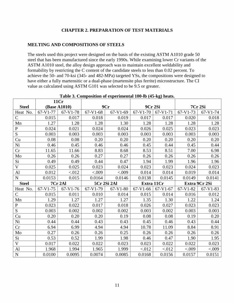
The steels used this project were designed on the basis of the existing ASTM A1010 grade 50 steel that has been manufactured since the early 1990s. While examining lower Cr variants of the ASTM A1010 steel, the alloy design approach was to maintain excellent weldability and formability by restricting the C content of the candidate steels to less than 0.02 percent. To achieve the 50- and 70-ksi (345- and 482-MPa) targeted YSs, the compositions were designed to have either a fully martensitic or a dual-phase (martensite plus ferrite) microstructure. The CI value as calculated using ASTM G101 was selected to be 9.5 or greater.

Table 3. Composition of experimental 100-lb (45-kg) heats.

Steel 11Cr

(Base A1010) 9Cr 9Cr 2Si 7Cr 2Si Heat No. 67-V1-77 67-V1-78 67-V1-68 67-V1-69 67-V1-70 67-V1-71 67-V1-73 67-V1-74 C 0.015 0.017 0.018 0.019 0.017 0.017 0.020 0.018 Mn 1.27 1.28 1.28 1.30 1.28 1.28 1.28 1.28 P 0.024 0.021 0.024 0.024 0.026 0.025 0.023 0.023 S 0.003 0.003 0.003 0.003 0.003 0.003 0.003 0.003 Cu 0.08 0.08 0.20 0.20 0.20 0.20 0.20 0.20 Ni 0.46 0.45 0.46 0.46 0.45 0.44 0.45 0.44 Cr 11.65 11.66 8.83 8.68 8.53 8.51 7.00 6.98 Mo 0.26 0.26 0.27 0.27 0.26 0.26 0.26 0.26 Si 0.49 0.49 0.44 0.47 1.94 1.99 1.96 1.96 V 0.025 0.025 0.023 0.024 0.023 0.023 0.024 0.023 Al 0.012 <.012 <.009 <.009 0.014 0.014 0.019 0.014 N 0.0153 0.015 0.0164 0.0146 0.0138 0.0145 0.0149 0.0141

Steel 7Cr 2Al 5Cr 2Si 2Al Extra 11Cr Extra 9Cr 2Si Heat No. 67-V1-75 67-V1-76 67-V1-79 67-V1-80 67-V1-66 67-V1-67 67-V1-82 67-V1-83 C 0.015 0.011 0.010 0.014 0.015 0.014 0.016 0.012 Mn 1.29 1.27 1.27 1.27 1.35 1.30 1.22 1.24 P 0.023 0.022 0.017 0.018 0.026 0.027 0.023 0.023 S 0.003 0.002 0.002 0.002 0.003 0.002 0.003 0.003 Cu 0.20 0.20 0.20 0.19 0.08 0.08 0.19 0.20 Ni 0.44 0.44 0.43 0.43 0.45 0.46 0.43 0.44 Cr 6.94 6.99 4.94 4.94 10.78 11.09 8.84 8.91 Mo 0.27 0.26 0.26 0.25 0.26 0.26 0.26 0.26 Si 0.53 0.52 1.99 1.98 0.46 0.47 1.90 1.95 V 0.017 0.022 0.022 0.023 0.023 0.022 0.022 0.023 Al 1.968 1.994 1.965 1.999 <.012 <.012 <.009 <.009 N 0.0100 0.0095 0.0074 0.0085 0.0168 0.0156 0.0157 0.0151

12

Melting was performed in an induction furnace under a vacuum. Originally, six 100-lb (45-kg) heats were scheduled to be cast, one heat for each steel. However, two or four heats of the steels were ultimately made to secure sufficient steel to perform all of the scheduled tests. The heats were all chemically analyzed to confirm that they complied with the targeted compositions. As shown in table 3, the compositions of the replicate heats of each steel are close. As a result, the replicates were treated as identical steels.

Each heat was poured in vacuo into iron molds. The resulting 100-lb (45-kg) ingots measured approximately 5 x 5 x 13 inches (125 x 125 x 350 mm). The ingots were prepared for rolling by milling opposite faces that would become the plate surfaces, trimming the side faces, and cutting off some of the hot top region.

HOT ROLLING

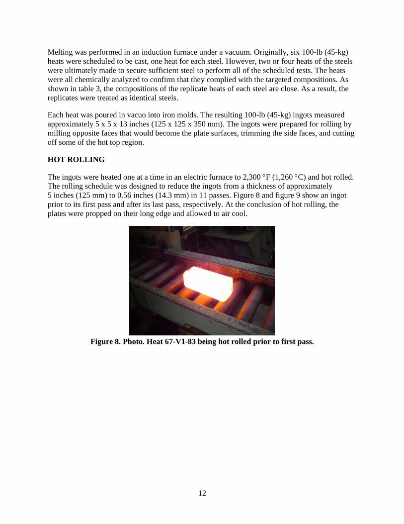
The ingots were heated one at a time in an electric furnace to 2,300 °F (1,260 °C) and hot rolled. The rolling schedule was designed to reduce the ingots from a thickness of approximately 5 inches (125 mm) to 0.56 inches (14.3 mm) in 11 passes. Figure 8 and figure 9 show an ingot prior to its first pass and after its last pass, respectively. At the conclusion of hot rolling, the plates were propped on their long edge and allowed to air cool.

Figure 8. Photo. Heat 67-V1-83 being hot rolled prior to first pass.

13

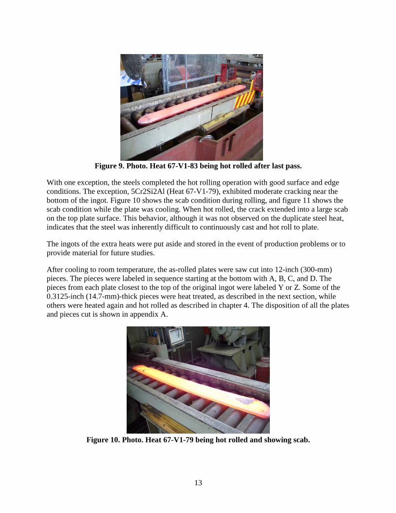
Figure 9. Photo. Heat 67-V1-83 being hot rolled after last pass.

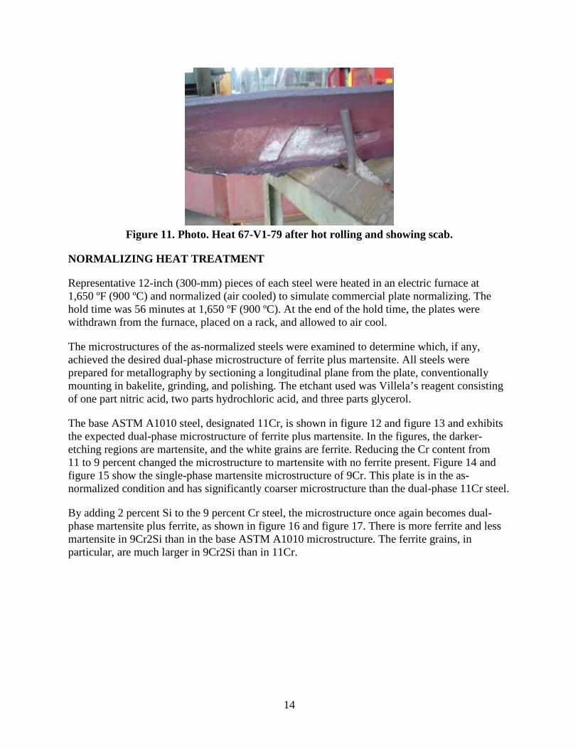
With one exception, the steels completed the hot rolling operation with good surface and edge conditions. The exception, 5Cr2Si2Al (Heat 67-V1-79), exhibited moderate cracking near the bottom of the ingot. Figure 10 shows the scab condition during rolling, and figure 11 shows the scab condition while the plate was cooling. When hot rolled, the crack extended into a large scab on the top plate surface. This behavior, although it was not observed on the duplicate steel heat, indicates that the steel was inherently difficult to continuously cast and hot roll to plate.

The ingots of the extra heats were put aside and stored in the event of production problems or to provide material for future studies.

After cooling to room temperature, the as-rolled plates were saw cut into 12-inch (300-mm) pieces. The pieces were labeled in sequence starting at the bottom with A, B, C, and D. The pieces from each plate closest to the top of the original ingot were labeled Y or Z. Some of the 0.3125-inch (14.7-mm)-thick pieces were heat treated, as described in the next section, while others were heated again and hot rolled as described in chapter 4. The disposition of all the plates and pieces cut is shown in appendix A.

Figure 10. Photo. Heat 67-V1-79 being hot rolled and showing scab.

14

Figure 11. Photo. Heat 67-V1-79 after hot rolling and showing scab.

NORMALIZING HEAT TREATMENT

Representative 12-inch (300-mm) pieces of each steel were heated in an electric furnace at 1,650 ºF (900 ºC) and normalized (air cooled) to simulate commercial plate normalizing. The hold time was 56 minutes at 1,650 ºF (900 ºC). At the end of the hold time, the plates were withdrawn from the furnace, placed on a rack, and allowed to air cool.

The microstructures of the as-normalized steels were examined to determine which, if any, achieved the desired dual-phase microstructure of ferrite plus martensite. All steels were prepared for metallography by sectioning a longitudinal plane from the plate, conventionally mounting in bakelite, grinding, and polishing. The etchant used was Villela’s reagent consisting of one part nitric acid, two parts hydrochloric acid, and three parts glycerol.

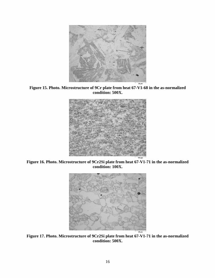
The base ASTM A1010 steel, designated 11Cr, is shown in figure 12 and figure 13 and exhibits the expected dual-phase microstructure of ferrite plus martensite. In the figures, the darker-etching regions are martensite, and the white grains are ferrite. Reducing the Cr content from 11 to 9 percent changed the microstructure to martensite with no ferrite present. Figure 14 and figure 15 show the single-phase martensite microstructure of 9Cr. This plate is in the as-normalized condition and has significantly coarser microstructure than the dual-phase 11Cr steel.

By adding 2 percent Si to the 9 percent Cr steel, the microstructure once again becomes dual-phase martensite plus ferrite, as shown in figure 16 and figure 17. There is more ferrite and less martensite in 9Cr2Si than in the base ASTM A1010 microstructure. The ferrite grains, in particular, are much larger in 9Cr2Si than in 11Cr.

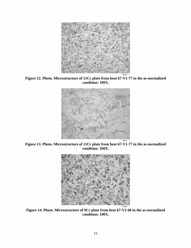
15

Figure 12. Photo. Microstructure of 11Cr plate from heat 67-V1-77 in the as-normalized

condition: 100X.

Figure 13. Photo. Microstructure of 11Cr plate from heat 67-V1-77 in the as-normalized

condition: 500X.

Figure 14. Photo. Microstructure of 9Cr plate from heat 67-V1-68 in the as-normalized

condition: 100X.

16

Figure 15. Photo. Microstructure of 9Cr plate from heat 67-V1-68 in the as-normalized

condition: 500X.

Figure 16. Photo. Microstructure of 9Cr2Si plate from heat 67-V1-71 in the as-normalized

condition: 100X.

Figure 17. Photo. Microstructure of 9Cr2Si plate from heat 67-V1-71 in the as-normalized

condition: 500X.

17

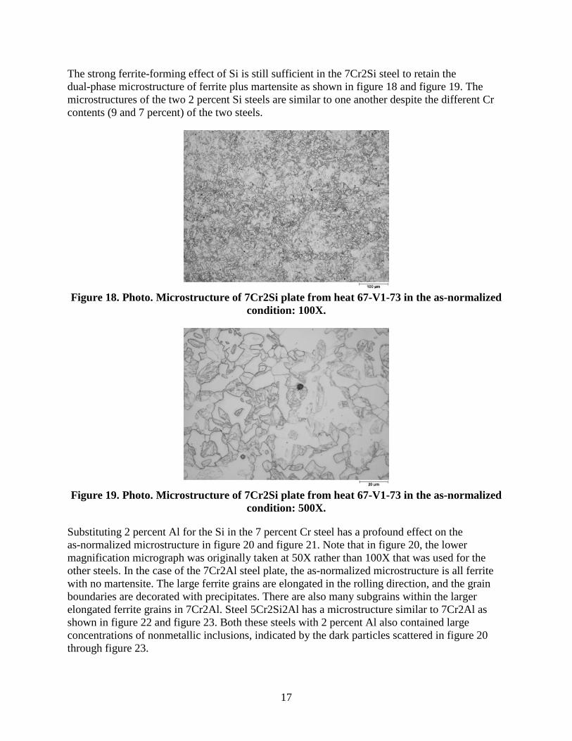
The strong ferrite-forming effect of Si is still sufficient in the 7Cr2Si steel to retain the dual-phase microstructure of ferrite plus martensite as shown in figure 18 and figure 19. The microstructures of the two 2 percent Si steels are similar to one another despite the different Cr contents (9 and 7 percent) of the two steels.

Figure 18. Photo. Microstructure of 7Cr2Si plate from heat 67-V1-73 in the as-normalized

condition: 100X.

Figure 19. Photo. Microstructure of 7Cr2Si plate from heat 67-V1-73 in the as-normalized

condition: 500X.

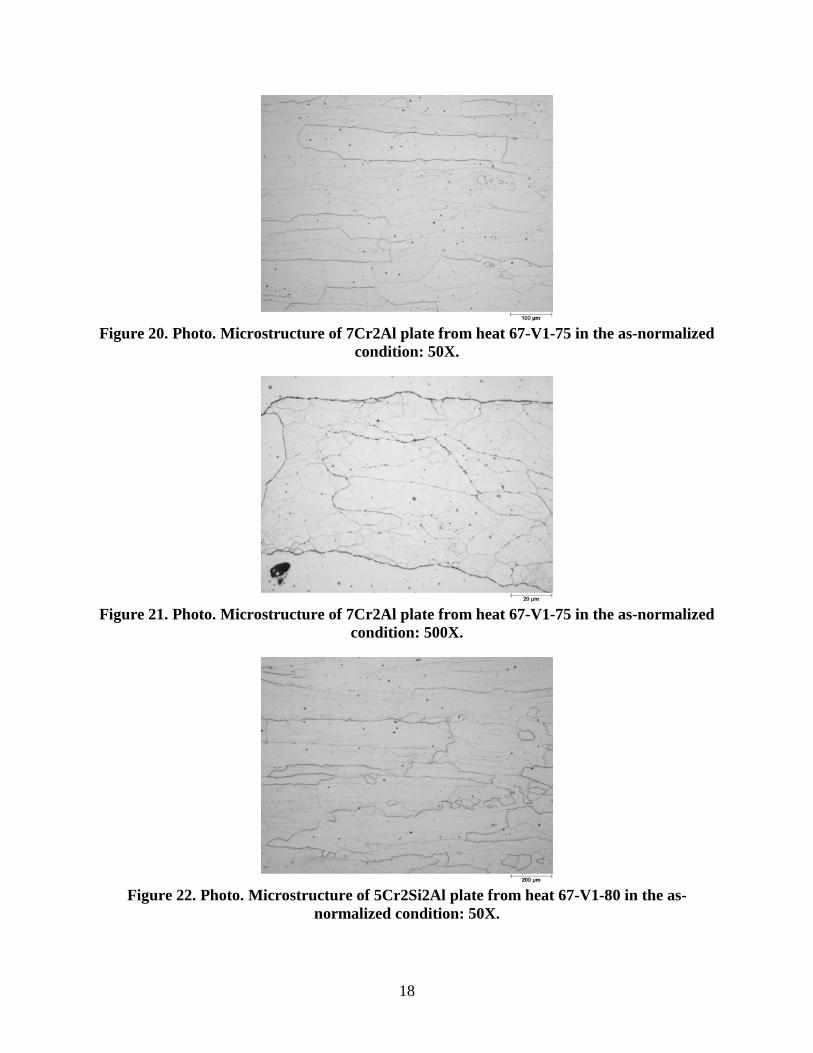
Substituting 2 percent Al for the Si in the 7 percent Cr steel has a profound effect on the as-normalized microstructure in figure 20 and figure 21. Note that in figure 20, the lower magnification micrograph was originally taken at 50X rather than 100X that was used for the other steels. In the case of the 7Cr2Al steel plate, the as-normalized microstructure is all ferrite with no martensite. The large ferrite grains are elongated in the rolling direction, and the grain boundaries are decorated with precipitates. There are also many subgrains within the larger elongated ferrite grains in 7Cr2Al. Steel 5Cr2Si2Al has a microstructure similar to 7Cr2Al as shown in figure 22 and figure 23. Both these steels with 2 percent Al also contained large concentrations of nonmetallic inclusions, indicated by the dark particles scattered in figure 20 through figure 23.

18

Figure 20. Photo. Microstructure of 7Cr2Al plate from heat 67-V1-75 in the as-normalized

condition: 50X.

Figure 21. Photo. Microstructure of 7Cr2Al plate from heat 67-V1-75 in the as-normalized

condition: 500X.

Figure 22. Photo. Microstructure of 5Cr2Si2Al plate from heat 67-V1-80 in the as-

normalized condition: 50X.

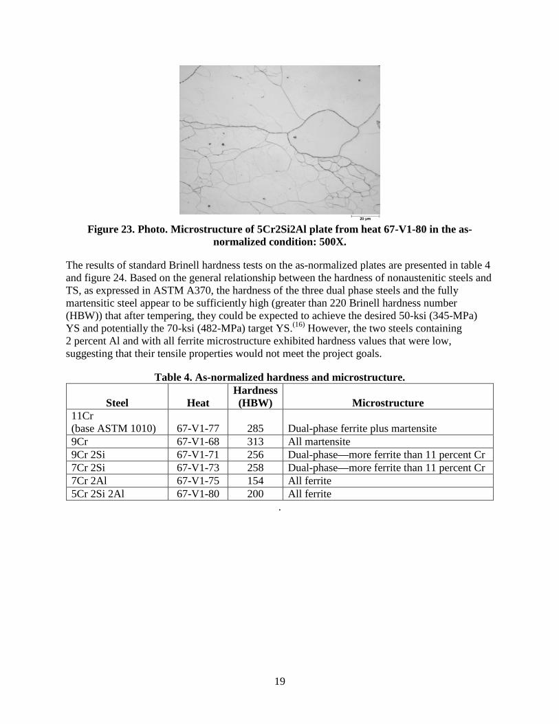
19

Figure 23. Photo. Microstructure of 5Cr2Si2Al plate from heat 67-V1-80 in the as-

normalized condition: 500X.

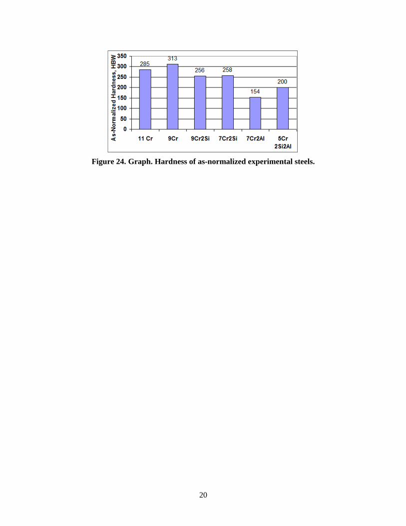
The results of standard Brinell hardness tests on the as-normalized plates are presented in table 4 and figure 24. Based on the general relationship between the hardness of nonaustenitic steels and TS, as expressed in ASTM A370, the hardness of the three dual phase steels and the fully martensitic steel appear to be sufficiently high (greater than 220 Brinell hardness number (HBW)) that after tempering, they could be expected to achieve the desired 50-ksi (345-MPa) YS and potentially the 70-ksi (482-MPa) target YS.(16) However, the two steels containing 2 percent Al and with all ferrite microstructure exhibited hardness values that were low, suggesting that their tensile properties would not meet the project goals.

Table 4. As-normalized hardness and microstructure.

Steel Heat Hardness (HBW) Microstructure

11Cr (base ASTM 1010) 67-V1-77 285 Dual-phase ferrite plus martensite 9Cr 67-V1-68 313 All martensite 9Cr 2Si 67-V1-71 256 Dual-phase—more ferrite than 11 percent Cr 7Cr 2Si 67-V1-73 258 Dual-phase—more ferrite than 11 percent Cr 7Cr 2Al 67-V1-75 154 All ferrite 5Cr 2Si 2Al 67-V1-80 200 All ferrite

.

20

Figure 24. Graph. Hardness of as-normalized experimental steels.

21

CHAPTER 3. MECHANICAL PROPERTIES OF TEST STEELS

TEMPERING STUDY TO ACHIEVE TARGETED STRENGTH

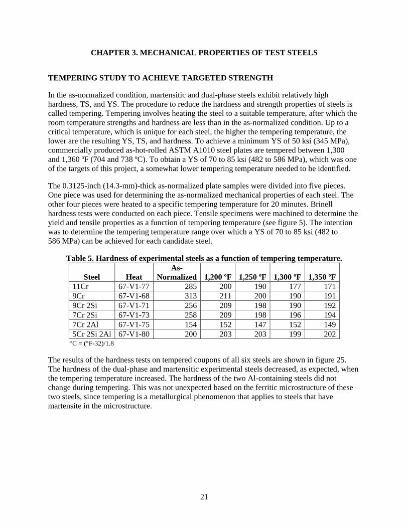
In the as-normalized condition, martensitic and dual-phase steels exhibit relatively high hardness, TS, and YS. The procedure to reduce the hardness and strength properties of steels is called tempering. Tempering involves heating the steel to a suitable temperature, after which the room temperature strengths and hardness are less than in the as-normalized condition. Up to a critical temperature, which is unique for each steel, the higher the tempering temperature, the lower are the resulting YS, TS, and hardness. To achieve a minimum YS of 50 ksi (345 MPa), commercially produced as-hot-rolled ASTM A1010 steel plates are tempered between 1,300 and 1,360 ºF (704 and 738 ºC). To obtain a YS of 70 to 85 ksi (482 to 586 MPa), which was one of the targets of this project, a somewhat lower tempering temperature needed to be identified.

The 0.3125-inch (14.3-mm)-thick as-normalized plate samples were divided into five pieces. One piece was used for determining the as-normalized mechanical properties of each steel. The other four pieces were heated to a specific tempering temperature for 20 minutes. Brinell hardness tests were conducted on each piece. Tensile specimens were machined to determine the yield and tensile properties as a function of tempering temperature (see figure 5). The intention was to determine the tempering temperature range over which a YS of 70 to 85 ksi (482 to 586 MPa) can be achieved for each candidate steel.

Table 5. Hardness of experimental steels as a function of tempering temperature.

Steel Heat As-

Normalized 1,200 ºF 1,250 ºF 1,300 ºF 1,350 ºF 11Cr 67-V1-77 285 200 190 177 171 9Cr 67-V1-68 313 211 200 190 191 9Cr 2Si 67-V1-71 256 209 198 190 192 7Cr 2Si 67-V1-73 258 209 198 196 194 7Cr 2Al 67-V1-75 154 152 147 152 149 5Cr 2Si 2Al 67-V1-80 200 203 203 199 202

°C = (°F-32)/1.8

The results of the hardness tests on tempered coupons of all six steels are shown in figure 25. The hardness of the dual-phase and martensitic experimental steels decreased, as expected, when the tempering temperature increased. The hardness of the two Al-containing steels did not change during tempering. This was not unexpected based on the ferritic microstructure of these two steels, since tempering is a metallurgical phenomenon that applies to steels that have martensite in the microstructure.

22

°C = (°F-32)/1.8

Figure 25. Graph. Hardness of the experimental steels after tempering.

The tensile properties of the 0.3125-inch (14.3-mm)-thick plates were measured using standard ASTM A370 round tensile specimens with a gauge diameter of 0.357 inches (9.1 mm) and a 1-inch (25.4-mm) gauge length.(16) The specimens were machined from the transverse direction of the plates, which is the standard orientation of tensile specimens made from commercially produced bridge plates. Crosshead speed was held constant throughout the tensile test at 0.080 inches per minutes (2 mm per minute). In addition to the standard tensile test quantities of 0.2 percent YS, ultimate TS, EL, and reduction of area (RA), the strain hardening coefficient (the n-value) was also calculated between strain values of 0.030 and the strain at the maximum load.

The as-normalized tensile properties of the six experimental steels are presented in table 6. The properties of the 11Cr steel are similar to a commercially produced ASTM A1010 as-normalized plate. This plate exhibited continuous yielding behavior, as expected for a dual-phase steel. The 9Cr steel, with its fully martensitic microstructure, was somewhat stronger than the 11Cr steel in the as-normalized condition, and it was consequently considerably less ductile. The tensile specimen unexpectedly broke after only 9 percent elongation. The two lower Cr steels with 2 percent Si had equal tensile behavior to each other, but these steels were considerably lower strength than the 11Cr and 9Cr steels. The YS of the two high Si steels was essentially 80 ksi (550 MPa) in the as-normalized condition. This is within one of the targeted YS ranges of 70 to 85 ksi (482 to 586 MPa). The 7Cr2Al steel had low tensile properties in the as-normalized condition. The as-normalized YS of this steel was just enough to achieve the 50- to 65-ksi (345- to 448-MPa) targeted YS range. A flaw in the tensile specimen caused it to fail outside the gauge length so no elongation value could be determined for this steel. However, the reduction in area value of only 14 percent indicates the steel has limited tensile ductility. Although the 5Cr2Si2Al steel is not as weak as the 7Cr2Al steel, its ductility is worse.

23

Table 6. Tensile properties of as-normalized steel plates.

Steel Hardness (HBW)

0.2 Percent YS (ksi)

TS (ksi)

EL (Percent)

RA (Percent) n-value Comment

11Cr 285 91.9 134.5 23.1 57.8 — Continuous yielding

9Cr 313 109.8 148.3 9.0 39.7 — Broke at 9 percent

9Cr2Si 256 80.4 121.7 29.6 64.0 0.118 Continuous yielding

7Cr2Si 258 79.1 121.1 29.9 68.8 0.120 Continuous yielding

7Cr2Al 154 54.5 70.2 — 14.0 0.173 Broke outside reduced section

5Cr2Si2Al 200 76.6 81.5 2.1 2.6 — Broke at 2.1 percent

1 ksi = 6.89 MPa — Indicates that the value could not be determined due to experimental difficulties.

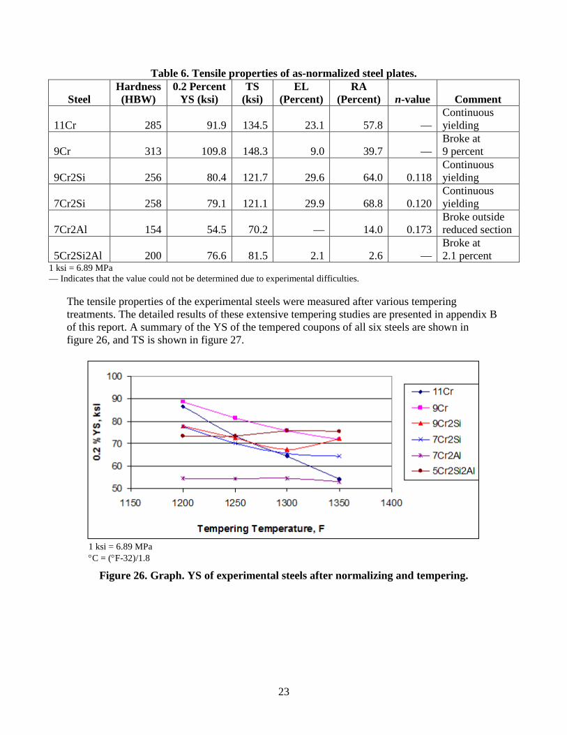
The tensile properties of the experimental steels were measured after various tempering treatments. The detailed results of these extensive tempering studies are presented in appendix B of this report. A summary of the YS of the tempered coupons of all six steels are shown in figure 26, and TS is shown in figure 27.

1 ksi = 6.89 MPa °C = (°F-32)/1.8

Figure 26. Graph. YS of experimental steels after normalizing and tempering.

24

1 ksi = 6.89 MPa °C = (°F-32)/1.8

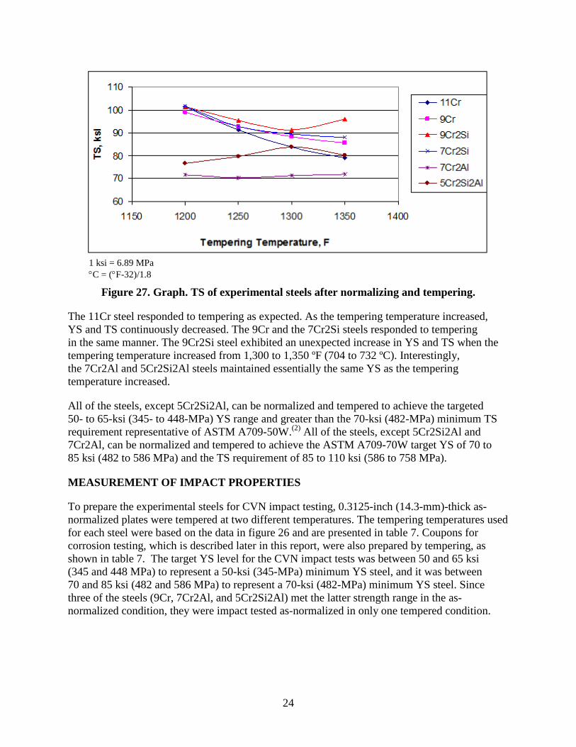
Figure 27. Graph. TS of experimental steels after normalizing and tempering.

The 11Cr steel responded to tempering as expected. As the tempering temperature increased, YS and TS continuously decreased. The 9Cr and the 7Cr2Si steels responded to tempering in the same manner. The 9Cr2Si steel exhibited an unexpected increase in YS and TS when the tempering temperature increased from 1,300 to 1,350 ºF (704 to 732 ºC). Interestingly, the 7Cr2Al and 5Cr2Si2Al steels maintained essentially the same YS as the tempering temperature increased.

All of the steels, except 5Cr2Si2Al, can be normalized and tempered to achieve the targeted 50- to 65-ksi (345- to 448-MPa) YS range and greater than the 70-ksi (482-MPa) minimum TS requirement representative of ASTM A709-50W.(2) All of the steels, except 5Cr2Si2Al and 7Cr2Al, can be normalized and tempered to achieve the ASTM A709-70W target YS of 70 to 85 ksi (482 to 586 MPa) and the TS requirement of 85 to 110 ksi (586 to 758 MPa).

MEASUREMENT OF IMPACT PROPERTIES

To prepare the experimental steels for CVN impact testing, 0.3125-inch (14.3-mm)-thick as-normalized plates were tempered at two different temperatures. The tempering temperatures used for each steel were based on the data in figure 26 and are presented in table 7. Coupons for corrosion testing, which is described later in this report, were also prepared by tempering, as shown in table 7. The target YS level for the CVN impact tests was between 50 and 65 ksi (345 and 448 MPa) to represent a 50-ksi (345-MPa) minimum YS steel, and it was between 70 and 85 ksi (482 and 586 MPa) to represent a 70-ksi (482-MPa) minimum YS steel. Since three of the steels (9Cr, 7Cr2Al, and 5Cr2Si2Al) met the latter strength range in the as-normalized condition, they were impact tested as-normalized in only one tempered condition.

25

Table 7. Tempering temperatures for CVN impact energy and corrosion studies.

Steel

Aim > 50 ksi YS Tempering

Temperature (ºF)

Aim > 70 ksi YS Tempering

Temperature (ºF) 11Cr 1,350 1,200 9Cr 1,350 As-normalized 9Cr2Si 1,350 1,200 7Cr2Si 1,350 1,200 7Cr2Al 1,200 As-normalized 5Cr2Si2Al 1,200 As-normalized

1 ksi = 6.89 MPa °C = (°F-32)/1.8

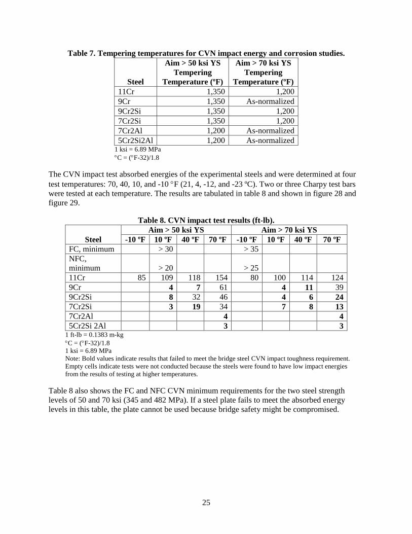
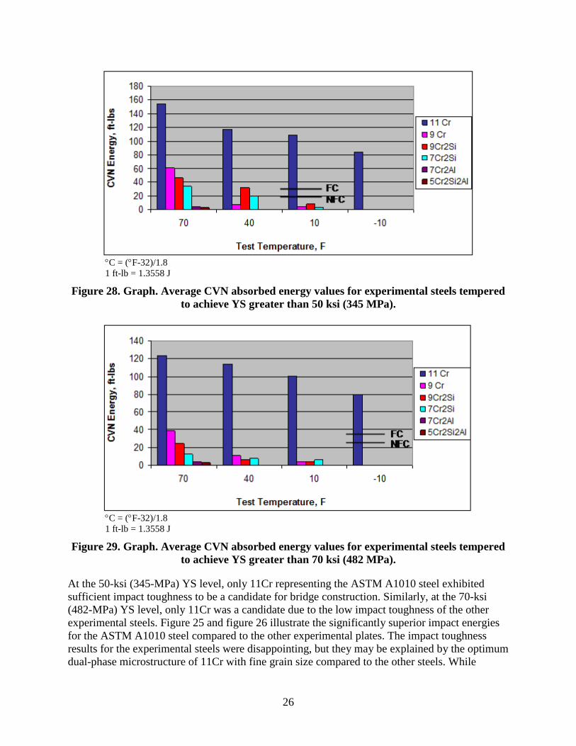
The CVN impact test absorbed energies of the experimental steels and were determined at four test temperatures: 70, 40, 10, and -10 °F (21, 4, -12, and -23 ºC). Two or three Charpy test bars were tested at each temperature. The results are tabulated in table 8 and shown in figure 28 and figure 29.

Table 8. CVN impact test results (ft-lb).

Steel Aim > 50 ksi YS Aim > 70 ksi YS

-10 ºF 10 ºF 40 ºF 70 ºF -10 ºF 10 ºF 40 ºF 70 ºF FC, minimum > 30 > 35 NFC, minimum > 20 > 25 11Cr 85 109 118 154 80 100 114 124 9Cr 4 7 61 4 11 39 9Cr2Si 8 32 46 4 6 24 7Cr2Si 3 19 34 7 8 13 7Cr2Al 4 4 5Cr2Si 2Al 3 3

1 ft-lb = 0.1383 m-kg °C = (°F-32)/1.8 1 ksi = 6.89 MPa Note: Bold values indicate results that failed to meet the bridge steel CVN impact toughness requirement. Empty cells indicate tests were not conducted because the steels were found to have low impact energies from the results of testing at higher temperatures.

Table 8 also shows the FC and NFC CVN minimum requirements for the two steel strength levels of 50 and 70 ksi (345 and 482 MPa). If a steel plate fails to meet the absorbed energy levels in this table, the plate cannot be used because bridge safety might be compromised.

26

°C = (°F-32)/1.8 1 ft-lb = 1.3558 J

Figure 28. Graph. Average CVN absorbed energy values for experimental steels tempered to achieve YS greater than 50 ksi (345 MPa).

°C = (°F-32)/1.8 1 ft-lb = 1.3558 J

Figure 29. Graph. Average CVN absorbed energy values for experimental steels tempered to achieve YS greater than 70 ksi (482 MPa).

At the 50-ksi (345-MPa) YS level, only 11Cr representing the ASTM A1010 steel exhibited sufficient impact toughness to be a candidate for bridge construction. Similarly, at the 70-ksi (482-MPa) YS level, only 11Cr was a candidate due to the low impact toughness of the other experimental steels. Figure 25 and figure 26 illustrate the significantly superior impact energies for the ASTM A1010 steel compared to the other experimental plates. The impact toughness results for the experimental steels were disappointing, but they may be explained by the optimum dual-phase microstructure of 11Cr with fine grain size compared to the other steels. While

27

further metallurgical development of the lower Cr steels is possible to improve impact toughness, it is desirable to determine the corrosion performance of the lower Cr steels to determine if there is a strong incentive for such work.

29

CHAPTER 4. PREPARATION OF CORROSION SPECIMENS

HOT ROLLING, NORMALIZING, AND TEMPERING TO ACHIEVE STRENGTH

As indicated earlier in this report, the 0.3125-inch (14.3-mm)-thick plates were saw cut into 12-inch (300-mm) lengths. To obtain material for corrosion testing, some of the pieces from each steel were reheated to 2,300 °F (1,260 °C) and hot rolled to sheets approximately 0.100 inches (2.5 mm) thick and 5 ft (1,500 mm) long. The specific pieces used for the corrosion specimens are shown in appendix A of this report. Hot rolling from 0.3125 to 0.100 inches (14.3 to 2.5 mm) produced generally good-quality steel plates (i.e., flat and with little or no cracking). This behavior was encouraging because there was some possibility that one or more of the experimental steels would exhibit poor hot workability.

The hot rolled sheets were sawcut into corrosion coupons measuring 4 inches (100 mm) by 6 inches (150 mm). Each as-rolled coupon was heated in an electric furnace under air atmosphere to 1,650 °F (900 °C), held 56 minutes, and air cooled to simulate commercial plate normalizing. The tempering temperatures used for the corrosion coupons were based on the data shown in figure 26 and are reported in table 7. The tempering time was 30 minutes.

31

CHAPTER 5. ACCELERATED LABORATORY CCTS

MODIFIED SAE J2334 TESTING

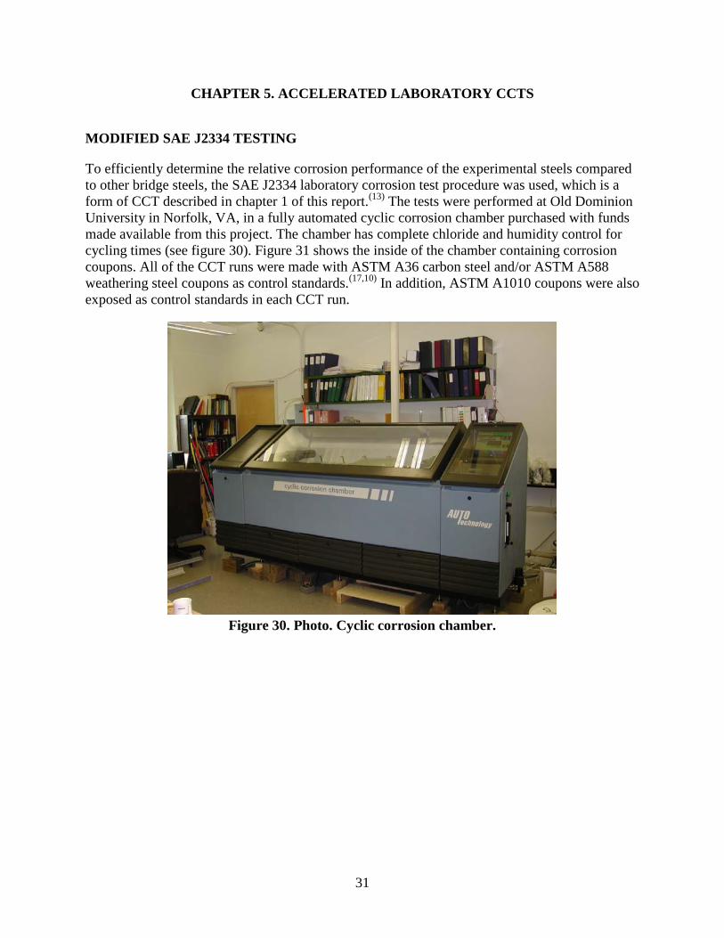
To efficiently determine the relative corrosion performance of the experimental steels compared to other bridge steels, the SAE J2334 laboratory corrosion test procedure was used, which is a form of CCT described in chapter 1 of this report.(13) The tests were performed at Old Dominion University in Norfolk, VA, in a fully automated cyclic corrosion chamber purchased with funds made available from this project. The chamber has complete chloride and humidity control for cycling times (see figure 30). Figure 31 shows the inside of the chamber containing corrosion coupons. All of the CCT runs were made with ASTM A36 carbon steel and/or ASTM A588 weathering steel coupons as control standards.(17,10) In addition, ASTM A1010 coupons were also exposed as control standards in each CCT run.

Figure 30. Photo. Cyclic corrosion chamber.

32

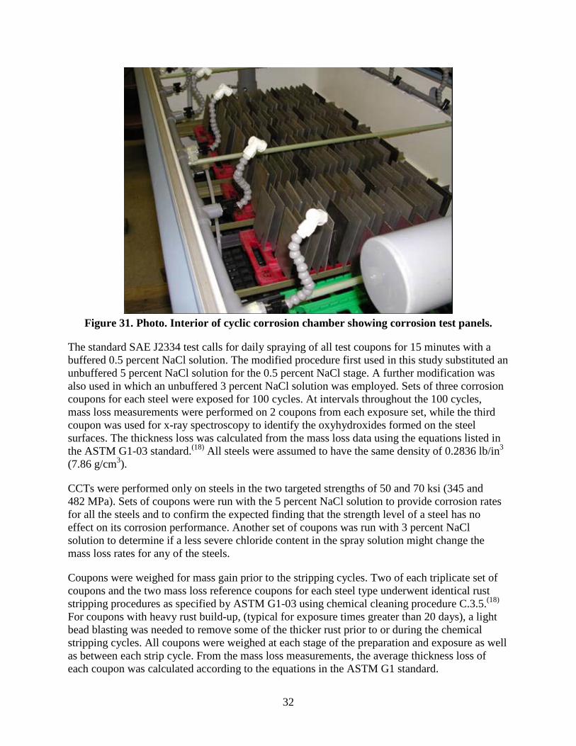
Figure 31. Photo. Interior of cyclic corrosion chamber showing corrosion test panels.

The standard SAE J2334 test calls for daily spraying of all test coupons for 15 minutes with a buffered 0.5 percent NaCl solution. The modified procedure first used in this study substituted an unbuffered 5 percent NaCl solution for the 0.5 percent NaCl stage. A further modification was also used in which an unbuffered 3 percent NaCl solution was employed. Sets of three corrosion coupons for each steel were exposed for 100 cycles. At intervals throughout the 100 cycles, mass loss measurements were performed on 2 coupons from each exposure set, while the third coupon was used for x-ray spectroscopy to identify the oxyhydroxides formed on the steel surfaces. The thickness loss was calculated from the mass loss data using the equations listed in the ASTM G1-03 standard.(18) All steels were assumed to have the same density of 0.2836 lb/in3 (7.86 g/cm3).

CCTs were performed only on steels in the two targeted strengths of 50 and 70 ksi (345 and 482 MPa). Sets of coupons were run with the 5 percent NaCl solution to provide corrosion rates for all the steels and to confirm the expected finding that the strength level of a steel has no effect on its corrosion performance. Another set of coupons was run with 3 percent NaCl solution to determine if a less severe chloride content in the spray solution might change the mass loss rates for any of the steels.

Coupons were weighed for mass gain prior to the stripping cycles. Two of each triplicate set of coupons and the two mass loss reference coupons for each steel type underwent identical rust stripping procedures as specified by ASTM G1-03 using chemical cleaning procedure C.3.5.(18) For coupons with heavy rust build-up, (typical for exposure times greater than 20 days), a light bead blasting was needed to remove some of the thicker rust prior to or during the chemical stripping cycles. All coupons were weighed at each stage of the preparation and exposure as well as between each strip cycle. From the mass loss measurements, the average thickness loss of each coupon was calculated according to the equations in the ASTM G1 standard.

33

CCT Data—5 Percent NaCl

The mass loss results for the experimental and reference steels are listed in table 9 and table 10, which give the total average thickness loss for each exposure period of each pair of steel coupons for the five exposure periods.

Table 9. Steels heat treated to more than 50 ksi (345 MPa) YS total thickness loss (mil).

Steel 0.2 Percent

YS (ksi) 10

Cycles 20

Cycles 40

Cycles 70

Cycles 100

Cycles ASTM A1010 control nd 0.24 0.61 2.0 4.0 4.7 11 Cr 73.1 0.45 1.0 2.3 4.0 6.7 9 Cr nd nd nd nd nd nd 9Cr2Si 75.4 0.72 2.1 5.5 12.0 21.5 7Cr2Si 65.0 1.0 3.1 10.0 21.4 31.0 7Cr2Al 52.2 1.3 2.9 7.2 10.1 15.2 5Cr2Si2Al 73.9 1.5 3.4 9.4 20.2 28.1 ASTM A588 control nd 2.2 10.0 22.0 35.4 52.4

1 ksi = 6.89 MPa 1 mil = 25.4 µ m nd = Not determined.

Table 10. Steels heat treated to more than 70 ksi (482 MPa) YS total thickness loss (mil).

Steel 0.2 Percent

YS (ksi) 10

Cycles 20

Cycles 40

Cycles 70

Cycles 100

Cycles 11Cr 90.4 0.17 0.52 1.8 3.3 6.3 9 Cr 81.2 1.0 2.9 6.3 9.9 14.8 9Cr2Si 79.0 0.84 2.0 5.8 13.7 22.0 7Cr2Si 78.8 1.0 3.0 10.5 23.3 31.6 7Cr2Al nd nd nd nd nd nd 5Cr2Si2Al nd nd nd nd nd nd

1 ksi = 6.89 MPa 1 mil = 25.4 µ m nd = Not determined.

Effect of Steel Strength

The effect of YS on the thickness loss for the 11Cr, 9Cr2Si, and 7Cr2Si steels is illustrated in figure 32 through figure 34. There is no consistent difference in thickness loss as a function of YS, and any differences that exist are small.

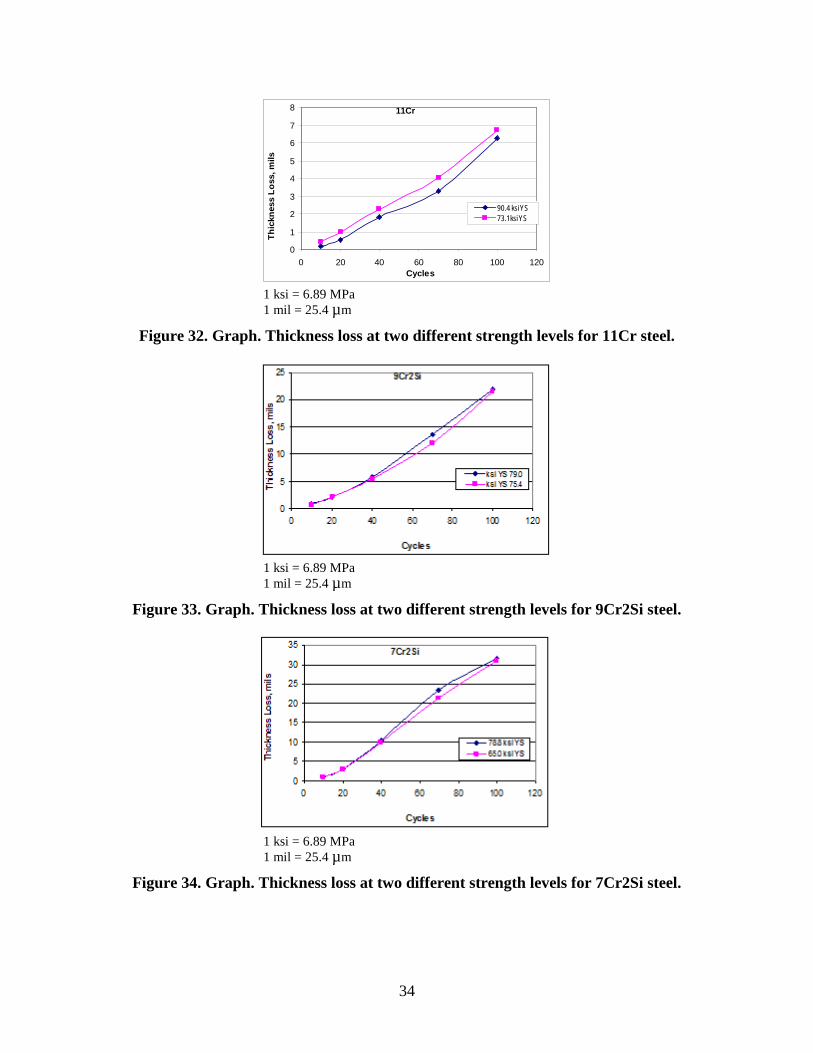
34

11Cr

0

1

2

3

4

5

6

7

8

0 20 40 60 80 100 120Cycles

Thic

knes

s Lo

ss, m

ils

90.4 ksi YS73.1 ksi YS

1 ksi = 6.89 MPa 1 mil = 25.4 µ m

Figure 32. Graph. Thickness loss at two different strength levels for 11Cr steel.

1 ksi = 6.89 MPa 1 mil = 25.4 µ m

Figure 33. Graph. Thickness loss at two different strength levels for 9Cr2Si steel.

1 ksi = 6.89 MPa 1 mil = 25.4 µ m

Figure 34. Graph. Thickness loss at two different strength levels for 7Cr2Si steel.

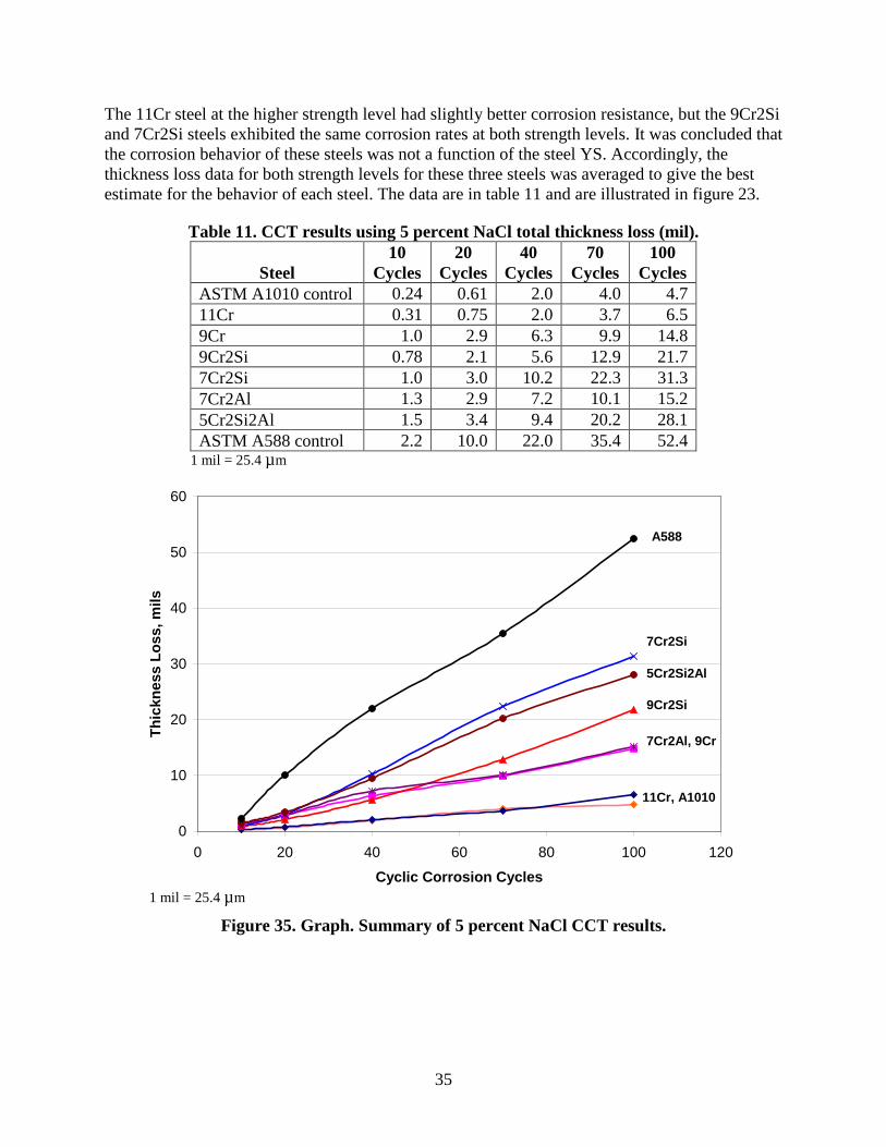
35

The 11Cr steel at the higher strength level had slightly better corrosion resistance, but the 9Cr2Si and 7Cr2Si steels exhibited the same corrosion rates at both strength levels. It was concluded that the corrosion behavior of these steels was not a function of the steel YS. Accordingly, the thickness loss data for both strength levels for these three steels was averaged to give the best estimate for the behavior of each steel. The data are in table 11 and are illustrated in figure 23.

Table 11. CCT results using 5 percent NaCl total thickness loss (mil).

Steel 10

Cycles 20

Cycles 40

Cycles 70

Cycles 100

Cycles ASTM A1010 control 0.24 0.61 2.0 4.0 4.7 11Cr 0.31 0.75 2.0 3.7 6.5 9Cr 1.0 2.9 6.3 9.9 14.8 9Cr2Si 0.78 2.1 5.6 12.9 21.7 7Cr2Si 1.0 3.0 10.2 22.3 31.3 7Cr2Al 1.3 2.9 7.2 10.1 15.2 5Cr2Si2Al 1.5 3.4 9.4 20.2 28.1 ASTM A588 control 2.2 10.0 22.0 35.4 52.4

1 mil = 25.4 µ m

0

10

20

30

40

50

60

0 20 40 60 80 100 120

Cyclic Corrosion Cycles

Thic

knes

s Lo

ss, m

ils

A588

7Cr2Si

5Cr2Si2Al

9Cr2Si

7Cr2Al, 9Cr

11Cr, A1010

1 mil = 25.4 µ m

Figure 35. Graph. Summary of 5 percent NaCl CCT results.

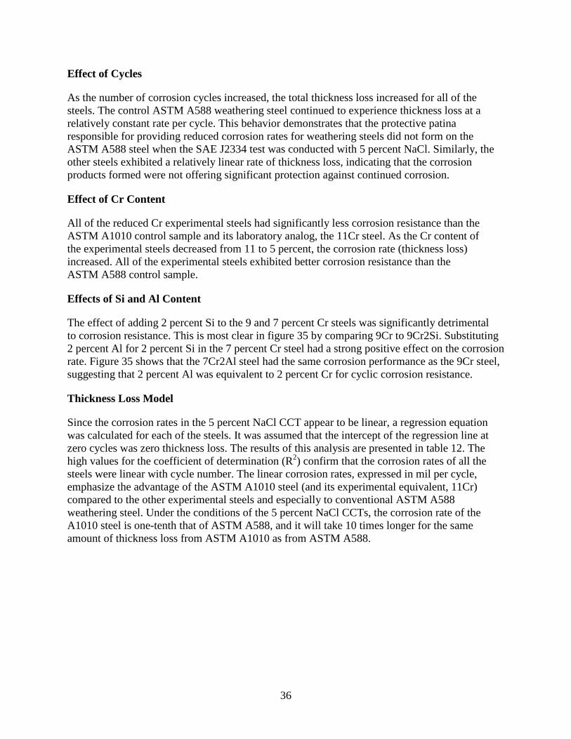
36

Effect of Cycles

As the number of corrosion cycles increased, the total thickness loss increased for all of the steels. The control ASTM A588 weathering steel continued to experience thickness loss at a relatively constant rate per cycle. This behavior demonstrates that the protective patina responsible for providing reduced corrosion rates for weathering steels did not form on the ASTM A588 steel when the SAE J2334 test was conducted with 5 percent NaCl. Similarly, the other steels exhibited a relatively linear rate of thickness loss, indicating that the corrosion products formed were not offering significant protection against continued corrosion.

Effect of Cr Content

All of the reduced Cr experimental steels had significantly less corrosion resistance than the ASTM A1010 control sample and its laboratory analog, the 11Cr steel. As the Cr content of the experimental steels decreased from 11 to 5 percent, the corrosion rate (thickness loss) increased. All of the experimental steels exhibited better corrosion resistance than the ASTM A588 control sample.

Effects of Si and Al Content

The effect of adding 2 percent Si to the 9 and 7 percent Cr steels was significantly detrimental to corrosion resistance. This is most clear in figure 35 by comparing 9Cr to 9Cr2Si. Substituting 2 percent Al for 2 percent Si in the 7 percent Cr steel had a strong positive effect on the corrosion rate. Figure 35 shows that the 7Cr2Al steel had the same corrosion performance as the 9Cr steel, suggesting that 2 percent Al was equivalent to 2 percent Cr for cyclic corrosion resistance.

Thickness Loss Model

Since the corrosion rates in the 5 percent NaCl CCT appear to be linear, a regression equation was calculated for each of the steels. It was assumed that the intercept of the regression line at zero cycles was zero thickness loss. The results of this analysis are presented in table 12. The high values for the coefficient of determination (R2) confirm that the corrosion rates of all the steels were linear with cycle number. The linear corrosion rates, expressed in mil per cycle, emphasize the advantage of the ASTM A1010 steel (and its experimental equivalent, 11Cr) compared to the other experimental steels and especially to conventional ASTM A588 weathering steel. Under the conditions of the 5 percent NaCl CCTs, the corrosion rate of the A1010 steel is one-tenth that of ASTM A588, and it will take 10 times longer for the same amount of thickness loss from ASTM A1010 as from ASTM A588.

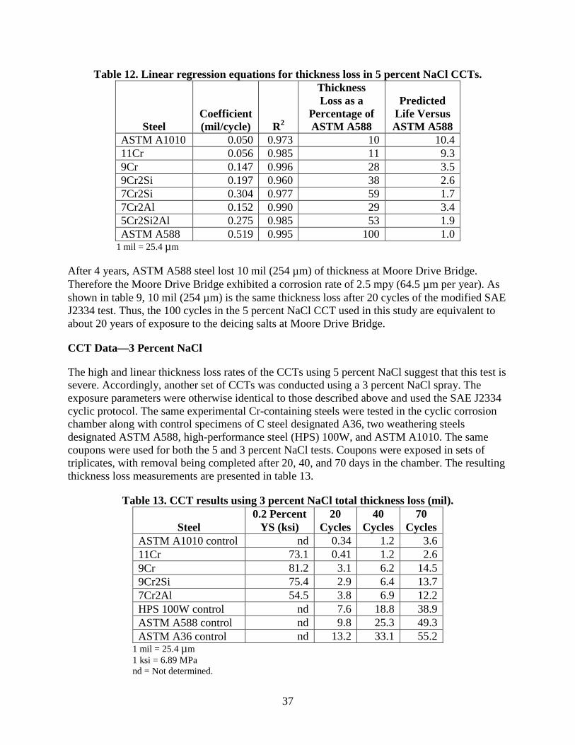
37

Table 12. Linear regression equations for thickness loss in 5 percent NaCl CCTs.

Steel

Coefficient (mil/cycle) R2

Thickness Loss as a

Percentage of ASTM A588

Predicted Life Versus ASTM A588

ASTM A1010 0.050 0.973 10 10.4 11Cr 0.056 0.985 11 9.3 9Cr 0.147 0.996 28 3.5 9Cr2Si 0.197 0.960 38 2.6 7Cr2Si 0.304 0.977 59 1.7 7Cr2Al 0.152 0.990 29 3.4 5Cr2Si2Al 0.275 0.985 53 1.9 ASTM A588 0.519 0.995 100 1.0

1 mil = 25.4 µ m

After 4 years, ASTM A588 steel lost 10 mil (254 µ m) of thickness at Moore Drive Bridge. Therefore the Moore Drive Bridge exhibited a corrosion rate of 2.5 mpy (64.5 µ m per year). As shown in table 9, 10 mil (254 µ m) is the same thickness loss after 20 cycles of the modified SAE J2334 test. Thus, the 100 cycles in the 5 percent NaCl CCT used in this study are equivalent to about 20 years of exposure to the deicing salts at Moore Drive Bridge.

CCT Data—3 Percent NaCl

The high and linear thickness loss rates of the CCTs using 5 percent NaCl suggest that this test is severe. Accordingly, another set of CCTs was conducted using a 3 percent NaCl spray. The exposure parameters were otherwise identical to those described above and used the SAE J2334 cyclic protocol. The same experimental Cr-containing steels were tested in the cyclic corrosion chamber along with control specimens of C steel designated A36, two weathering steels designated ASTM A588, high-performance steel (HPS) 100W, and ASTM A1010. The same coupons were used for both the 5 and 3 percent NaCl tests. Coupons were exposed in sets of triplicates, with removal being completed after 20, 40, and 70 days in the chamber. The resulting thickness loss measurements are presented in table 13.

Table 13. CCT results using 3 percent NaCl total thickness loss (mil).

Steel 0.2 Percent

YS (ksi) 20

Cycles 40

Cycles 70

Cycles ASTM A1010 control nd 0.34 1.2 3.6 11Cr 73.1 0.41 1.2 2.6 9Cr 81.2 3.1 6.2 14.5 9Cr2Si 75.4 2.9 6.4 13.7 7Cr2Al 54.5 3.8 6.9 12.2 HPS 100W control nd 7.6 18.8 38.9 ASTM A588 control nd 9.8 25.3 49.3 ASTM A36 control nd 13.2 33.1 55.2

1 mil = 25.4 µ m 1 ksi = 6.89 MPa nd = Not determined.

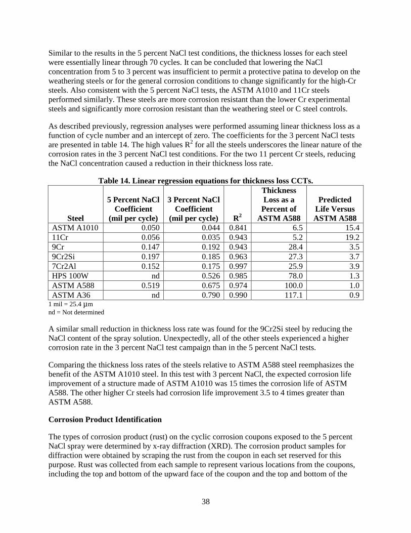
38

Similar to the results in the 5 percent NaCl test conditions, the thickness losses for each steel were essentially linear through 70 cycles. It can be concluded that lowering the NaCl concentration from 5 to 3 percent was insufficient to permit a protective patina to develop on the weathering steels or for the general corrosion conditions to change significantly for the high-Cr steels. Also consistent with the 5 percent NaCl tests, the ASTM A1010 and 11Cr steels performed similarly. These steels are more corrosion resistant than the lower Cr experimental steels and significantly more corrosion resistant than the weathering steel or C steel controls.

As described previously, regression analyses were performed assuming linear thickness loss as a function of cycle number and an intercept of zero. The coefficients for the 3 percent NaCl tests are presented in table 14. The high values R2 for all the steels underscores the linear nature of the corrosion rates in the 3 percent NaCl test conditions. For the two 11 percent Cr steels, reducing the NaCl concentration caused a reduction in their thickness loss rate.

Table 14. Linear regression equations for thickness loss CCTs.

Steel

5 Percent NaCl Coefficient

(mil per cycle)

3 Percent NaCl Coefficient

(mil per cycle)

R2

Thickness Loss as a

Percent of ASTM A588

Predicted

Life Versus ASTM A588

ASTM A1010 0.050 0.044 0.841 6.5 15.4 11Cr 0.056 0.035 0.943 5.2 19.2 9Cr 0.147 0.192 0.943 28.4 3.5 9Cr2Si 0.197 0.185 0.963 27.3 3.7 7Cr2Al 0.152 0.175 0.997 25.9 3.9 HPS 100W nd 0.526 0.985 78.0 1.3 ASTM A588 0.519 0.675 0.974 100.0 1.0 ASTM A36 nd 0.790 0.990 117.1 0.9

1 mil = 25.4 µ m nd = Not determined

A similar small reduction in thickness loss rate was found for the 9Cr2Si steel by reducing the NaCl content of the spray solution. Unexpectedly, all of the other steels experienced a higher corrosion rate in the 3 percent NaCl test campaign than in the 5 percent NaCl tests.

Comparing the thickness loss rates of the steels relative to ASTM A588 steel reemphasizes the benefit of the ASTM A1010 steel. In this test with 3 percent NaCl, the expected corrosion life improvement of a structure made of ASTM A1010 was 15 times the corrosion life of ASTM A588. The other higher Cr steels had corrosion life improvement 3.5 to 4 times greater than ASTM A588.

Corrosion Product Identification

The types of corrosion product (rust) on the cyclic corrosion coupons exposed to the 5 percent NaCl spray were determined by x-ray diffraction (XRD). The corrosion product samples for diffraction were obtained by scraping the rust from the coupon in each set reserved for this purpose. Rust was collected from each sample to represent various locations from the coupons, including the top and bottom of the upward face of the coupon and the top and bottom of the

39

downward face. In some cases where there was only thin rust on the coupon, the rust powder was collected from the upward-facing coupon surface (UA) and all of the downward-facing coupon surface (DA). There were instances when it was possible to collect outer and inner rust layers, and those were reserved for possible future analysis beyond the scope of the present study. The collected rust was ground to a powder less than 4.87 mil (125 µ m).

All XRD patterns were recorded using a PANalytical XPert PRO x-ray diffractometer. The powder samples were held in a spinning automated sample changer and exposed to cobalt x-rays (wavelength = 1.78901 Å ) with an iron filter. The x-ray tube operated at 45 kV and 40 mA. The scan was generally between 10 to 80 degrees (2 theta) with an angular step size of 0.0170 degrees and total run time of 9 h 26 minutes or 4 h 43 minutes. The resulting patterns were analyzed using PANalytical software XPert Highscore Plus using ICDD® PDF®-4 database to identify standard XRD patterns for known iron oxides.(19)

To measure the chloride content of the rust, XRD data were recorded on the same powder samples using Thermo Scientific Niton portable x-ray fluorescence (XRF) spectrometer model XL3t 900S GOLDD, which is sensitive to elements whose atomic number is below that of Cl. Diffraction data were recorded for 80 to 160 s per sample. The diffraction patterns were calibrated using Nitron standards.

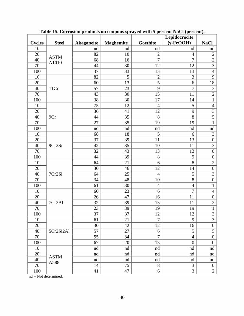
40

Table 15. Corrosion products on coupons sprayed with 5 percent NaCl (percent).

Cycles Steel Akaganeite Maghemite Goethite Lepidocrocite

(γ -FeOOH) NaCl 10

ASTM A1010

nd nd nd nd nd 20 82 10 2 4 2 40 68 16 7 7 2 70 44 30 12 12 3 100 37 33 13 13 4 10

11Cr

82 5 2 3 9 20 60 13 5 6 18 40 57 23 9 7 3 70 43 30 15 11 2 100 38 30 17 14 1 10

9Cr

75 12 4 5 4 20 36 41 12 9 3 40 44 35 8 8 5 70 27 35 19 19 1 100 nd nd nd nd nd 10

9Cr2Si

68 18 5 6 3 20 37 39 11 13 0 40 42 35 10 11 3 70 32 43 13 12 0 100 44 39 8 9 0 10

7Cr2Si

64 21 6 8 2 20 30 46 12 14 0 40 64 25 4 5 3 70 34 48 10 8 0 100 61 30 4 4 1 10

7Cr2Al

60 23 6 7 4 20 26 47 16 11 0 40 32 39 15 11 2 70 23 39 19 19 1 100 37 37 12 12 3 10

5Cr2Si2Al

61 21 7 9 3 20 30 42 12 16 0 40 57 27 6 5 5 70 55 34 7 4 0 100 67 20 13 0 0 10

ASTM A588

nd nd nd nd nd 20 nd nd nd nd nd 40 nd nd nd nd nd 70 14 75 8 3 0 100 41 47 6 3 2

nd = Not determined.

41

The results of the analyses of corrosion products on the cyclic corrosion coupons with 5 percent NaCl as the spray solution are summarized in table 15. Individual results are in appendix C of this report. There is considerable scatter in the data, but a few trends were identified. First, as the cyclic corrosion cycles increased, most of the steels exhibited a general trend where the amount of akaganeite declined and was replaced by the other oxyhydroxides maghemite, goethite, and lepidocrocite. Second, the overall amount of goethite and lepidocrocite was equal for all the steels, so these corrosion products were not responsible for the significant difference in the CCT corrosion rates among the various steels. Third, almost all the corrosion product samples contained traces of NaCl.

The overall average corrosion products for each of the steels is presented in table 16. This table is derived from table 15 by averaging the corrosion products throughout the CCT cycles. The corrosion product of the two 11 percent Cr steels contains significantly less maghemite than the steels with lower Cr content. Instead, the 11 percent Cr steels have the highest akaganeite levels. This is the reason for the significantly better corrosion rates observed for the 11 percent Cr steels.

Table 16. Overall average corrosion products from 5 percent NaCl CCTs (percent). Steel Akaganeite Maghemite Goethite Lepidocrocite NaCl

ASTM A1010 58 22 8 9 3 11Cr 56 20 10 8 6 9Cr 45 31 11 10 3 9Cr2Si 45 35 9 10 1 7Cr2Si 51 34 7 7 1 7Cr2Al 36 37 14 12 2 5Cr2Si2Al 54 29 9 7 1

As the Cr content of the steels decreased, the percentage of maghemite in the corrosion product increased. As noted previously, the percentage of goethite and lepidocrocite remained approximately equal for all of the Cr-containing steels, which contrasts with ASTM A588, which had very little lepidocrocite. It has been shown that in high-chloride bridge environments, ASTM A588 rust is coarse goethite and akaganeite with no lepidocrocite.(20) The CCT behavior of the ASTM A588 samples are consistent with reported behavior of the steel in severe chloride bridge service.

The CCT protocol provides a high time-of-wetness, which promotes the corrosion product maghemite to form at the steel/rust interface in the presence or absence of chlorides. This is the same type of corrosion product observed on corroding steels submerged in the ocean. The high time-of-wetness decreases oxygen availability to form akaganeite. However, akaganeite is sometimes present in smaller amounts due to the surface of the rust drying during the CCT dry cycle. Once the rust thickens, drying at the steel surface under the thick rust is limited, and a high corrosion rate continues with maghemite formation. At the surface of the steel beneath the rust, an anaerobic environment exists and causes blisters with low pH to form in the presence of chloride. Blistered regions on a few of the corrosion coupons were analyzed (see appendix C of this report), and FeCl2x4H2O was found inside the blisters at pH = 2. As will be shown in the next chapter, the CCT exposure conditions do not adequately mimic the severe chloride bridge conditions at the Moore Drive Bridge. The corrosion product on ASTM A588 from the

42

Moore Drive Bridge does not show any maghemite corrosion product because the bridge does not have high time-of-wetness.

Overall, the rust compositions for the experimental Cr steel samples with less than 11 percent Cr were similar and contained more corrosion product maghemite. The 5 percent NaCl spray solution CCT and the 3 percent NaCl tests created an aggressively corrosive environment with excessively high time-of-wetness. Because the corrosion products that form on the experimental Cr steel samples subjected to the CCT have high maghemite volumes and maghemite is not present in the corrosion products of the Moore Drive Bridge, the corrosion rates measured by the CCTs may not be representative of actual bridge service.

43

CHAPTER 6. ONE-YEAR FIELD TEST AT SEVERE HIGHWAY CORROSION SITE

The CCTs provided important data on the relative corrosion of the experimental and control steels in the laboratory test. The outcomes of the CCTs are represented in thickness loss per corrosion cycle. To predict thickness loss in a severe high-chloride bridge environment, three of the experimental steels were exposed to actual bridge service at the Moore Drive Bridge over I-394 S in Rochester, NY. ASTM A1010 and ASTM A588 have been studied previously at the Moore Drive Bridge.(11)

The mechanical property results described previously showed that only ASTM A1010 steel is a candidate for bridge construction. However, the CCTs results showed a strong positive effect of Cr, a strong negative effect of Si, and a strong positive effect of Al. The steels selected for exposure on the Moore Drive Bridge were 9Cr, 7Cr2Si, and 7Cr2Al. By testing these three steels, it was hoped that insights could be made on the relative atmospheric corrosion resistance of Cr, Si, and Al alloy additions to high-Cr steel in an adverse outdoor environment.

To accommodate the test racks on the Moore Drive Bridge, standard 4- x 6- x 0.100-inch (106- x 152- x 2.54-mm) coupons were cut in half to create 4- x 3- x 0.100-inch (106- x 76- x 2.54-mm) coupons. The Moore Drive Bridge has racks in three separate locations relative to the roadway. Racks 1 and 2 are near the abutment and over the roadway, respectively. Studies have shown that the corrosion behavior on racks 1 and 2 are similar. Rack 3 over the Erie Canal and more than 100 ft (30 m) away from the roadway provides a significantly different microclimate for atmospheric corrosion testing. Due to space constraints on racks 1 and 2, the coupons for the present study were distributed between these two racks. Triplicate specimens were placed on the bridge on November 18, 2008.

Prior to removal from the Moore Drive Bridge on October 13, 2009, the coupons were photographed on their racks (see figure 36). Following storage in the laboratory for 3 days, the coupons were weighed to determine mass gain. XRF spectrometry was used to determine elemental composition, including chloride, of the surface rust at several locations on each surface of each coupon. XRF had also been used to analyze elemental composition of the rust on webs and flanges of Moore Drive Bridge near the exposure racks.

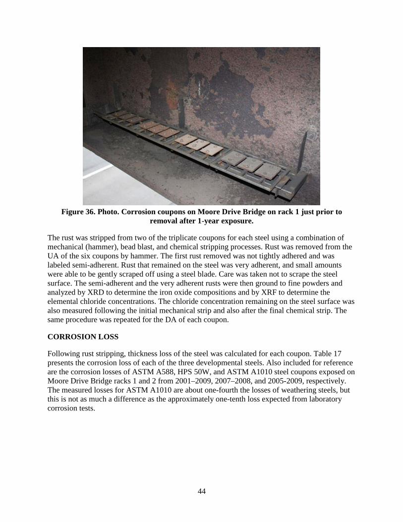
44

Figure 36. Photo. Corrosion coupons on Moore Drive Bridge on rack 1 just prior to

removal after 1-year exposure.

The rust was stripped from two of the triplicate coupons for each steel using a combination of mechanical (hammer), bead blast, and chemical stripping processes. Rust was removed from the UA of the six coupons by hammer. The first rust removed was not tightly adhered and was labeled semi-adherent. Rust that remained on the steel was very adherent, and small amounts were able to be gently scraped off using a steel blade. Care was taken not to scrape the steel surface. The semi-adherent and the very adherent rusts were then ground to fine powders and analyzed by XRD to determine the iron oxide compositions and by XRF to determine the elemental chloride concentrations. The chloride concentration remaining on the steel surface was also measured following the initial mechanical strip and also after the final chemical strip. The same procedure was repeated for the DA of each coupon.

CORROSION LOSS

Following rust stripping, thickness loss of the steel was calculated for each coupon. Table 17 presents the corrosion loss of each of the three developmental steels. Also included for reference are the corrosion losses of ASTM A588, HPS 50W, and ASTM A1010 steel coupons exposed on Moore Drive Bridge racks 1 and 2 from 2001–2009, 2007–2008, and 2005-2009, respectively. The measured losses for ASTM A1010 are about one-fourth the losses of weathering steels, but this is not as much a difference as the approximately one-tenth loss expected from laboratory corrosion tests.

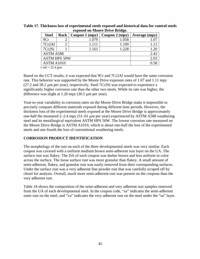
45

Table 17. Thickness loss of experimental steels exposed and historical data for control steels exposed on Moore Drive Bridge.

Steel Rack Coupon 1 (mpy) Coupon 2 (mpy) Average (mpy) 9Cr 2 1.079 1.058 1.07 7Cr2Al 2 1.111 1.109 1.11 7Cr2Si 1 1.161 1.228 1.20 ASTM A588 2.43 ASTM HPS 50W 2.03 ASTM A1010 0.58

1 mil = 25.4 µ m

Based on the CCT results, it was expected that 9Cr and 7Cr2Al would have the same corrosion rate. This behavior was supported by the Moore Drive exposure rates of 1.07 and 1.11 mpy (27.2 and 28.2 µ m per year), respectively. Steel 7Cr2Si was expected to experience a significantly higher corrosion rate than the other two steels. While its rate was higher, the difference was slight at 1.20 mpy (30.5 µ m per year).

Year-to-year variability in corrosion rates on the Moore Drive Bridge make it impossible to precisely compare different materials exposed during different time periods. However, the thickness loss of the experimental steels exposed at the Moore Drive Bridge is approximately one-half the measured 2–2.4 mpy (51–61 µ m per year) experienced by ASTM A588 weathering steel and its metallurgical equivalent ASTM HPS 50W. The lowest corrosion rate measured on the Moore Drive Bridge is ASTM A1010, which is about one-half the loss of the experimental steels and one-fourth the loss of conventional weathering steels.

CORROSION PRODUCT IDENTIFICATION

The morphology of the rust on each of the three developmental steels was very similar. Each coupon was covered with a uniform medium brown semi-adherent rust layer on the UA. The surface rust was flakey. The DA of each coupon was darker brown and less uniform in color across the surface. The loose surface rust was more granular than flakey. A small amount of semi-adherent, flakey, and granular rust was easily removed from their corresponding surfaces. Under the surface rust was a very adherent fine powder rust that was carefully scraped off by chisel for analysis. Overall, much more semi-adherent rust was present on the coupons than the very adherent rust.

Table 18 shows the composition of the semi-adherent and very adherent rust samples removed from the UA of each developmental steel. In the coupon code, “sa” indicates the semi-adherent outer rust on the steel, and “va” indicates the very adherent rust on the steel under the “sa” layer.

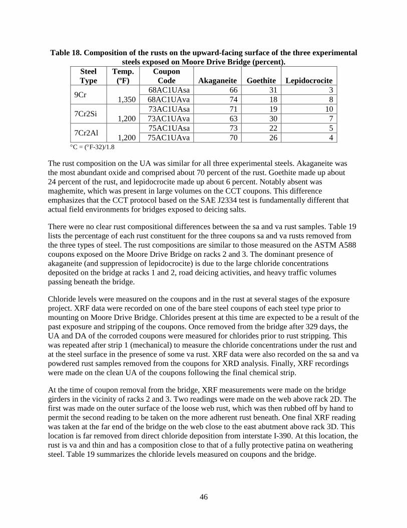
46

Table 18. Composition of the rusts on the upward-facing surface of the three experimental steels exposed on Moore Drive Bridge (percent).

Steel Type

Temp. (ºF)

Coupon Code Akaganeite Goethite Lepidocrocite

9Cr 1,350 68AC1UAsa 66 31 3 68AC1UAva 74 18 8

7Cr2Si 1,200 73AC1UAsa 71 19 10 73AC1UAva 63 30 7

7Cr2Al 1,200 75AC1UAsa 73 22 5 75AC1UAva 70 26 4

°C = (°F-32)/1.8

The rust composition on the UA was similar for all three experimental steels. Akaganeite was the most abundant oxide and comprised about 70 percent of the rust. Goethite made up about 24 percent of the rust, and lepidocrocite made up about 6 percent. Notably absent was maghemite, which was present in large volumes on the CCT coupons. This difference emphasizes that the CCT protocol based on the SAE J2334 test is fundamentally different that actual field environments for bridges exposed to deicing salts.

There were no clear rust compositional differences between the sa and va rust samples. Table 19 lists the percentage of each rust constituent for the three coupons sa and va rusts removed from the three types of steel. The rust compositions are similar to those measured on the ASTM A588 coupons exposed on the Moore Drive Bridge on racks 2 and 3. The dominant presence of akaganeite (and suppression of lepidocrocite) is due to the large chloride concentrations deposited on the bridge at racks 1 and 2, road deicing activities, and heavy traffic volumes passing beneath the bridge.

Chloride levels were measured on the coupons and in the rust at several stages of the exposure project. XRF data were recorded on one of the bare steel coupons of each steel type prior to mounting on Moore Drive Bridge. Chlorides present at this time are expected to be a result of the past exposure and stripping of the coupons. Once removed from the bridge after 329 days, the UA and DA of the corroded coupons were measured for chlorides prior to rust stripping. This was repeated after strip 1 (mechanical) to measure the chloride concentrations under the rust and at the steel surface in the presence of some va rust. XRF data were also recorded on the sa and va powdered rust samples removed from the coupons for XRD analysis. Finally, XRF recordings were made on the clean UA of the coupons following the final chemical strip.

At the time of coupon removal from the bridge, XRF measurements were made on the bridge girders in the vicinity of racks 2 and 3. Two readings were made on the web above rack 2D. The first was made on the outer surface of the loose web rust, which was then rubbed off by hand to permit the second reading to be taken on the more adherent rust beneath. One final XRF reading was taken at the far end of the bridge on the web close to the east abutment above rack 3D. This location is far removed from direct chloride deposition from interstate I-390. At this location, the rust is va and thin and has a composition close to that of a fully protective patina on weathering steel. Table 19 summarizes the chloride levels measured on coupons and the bridge.

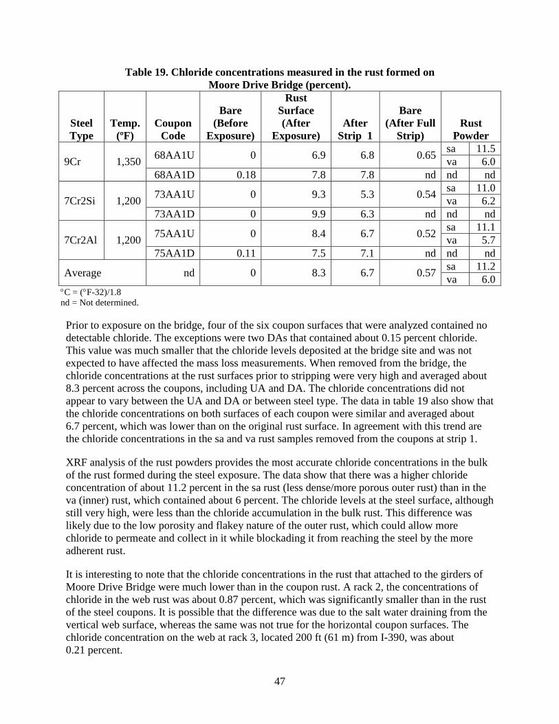
47

Table 19. Chloride concentrations measured in the rust formed on Moore Drive Bridge (percent).

Steel Type

Temp.

(ºF)

Coupon

Code

Bare (Before

Exposure)

Rust Surface (After

Exposure)

After

Strip 1

Bare (After Full

Strip)

Rust

Powder

9Cr 1,350 68AA1U 0 6.9 6.8 0.65 sa 11.5 va 6.0

68AA1D 0.18 7.8 7.8 nd nd nd

7Cr2Si 1,200 73AA1U 0 9.3 5.3 0.54 sa 11.0 va 6.2

73AA1D 0 9.9 6.3 nd nd nd

7Cr2Al 1,200 75AA1U 0 8.4 6.7 0.52 sa 11.1 va 5.7

75AA1D 0.11 7.5 7.1 nd nd nd

Average nd 0 8.3 6.7 0.57 sa 11.2 va 6.0

°C = (°F-32)/1.8 nd = Not determined.

Prior to exposure on the bridge, four of the six coupon surfaces that were analyzed contained no detectable chloride. The exceptions were two DAs that contained about 0.15 percent chloride. This value was much smaller that the chloride levels deposited at the bridge site and was not expected to have affected the mass loss measurements. When removed from the bridge, the chloride concentrations at the rust surfaces prior to stripping were very high and averaged about 8.3 percent across the coupons, including UA and DA. The chloride concentrations did not appear to vary between the UA and DA or between steel type. The data in table 19 also show that the chloride concentrations on both surfaces of each coupon were similar and averaged about 6.7 percent, which was lower than on the original rust surface. In agreement with this trend are the chloride concentrations in the sa and va rust samples removed from the coupons at strip 1.

XRF analysis of the rust powders provides the most accurate chloride concentrations in the bulk of the rust formed during the steel exposure. The data show that there was a higher chloride concentration of about 11.2 percent in the sa rust (less dense/more porous outer rust) than in the va (inner) rust, which contained about 6 percent. The chloride levels at the steel surface, although still very high, were less than the chloride accumulation in the bulk rust. This difference was likely due to the low porosity and flakey nature of the outer rust, which could allow more chloride to permeate and collect in it while blockading it from reaching the steel by the more adherent rust.

It is interesting to note that the chloride concentrations in the rust that attached to the girders of Moore Drive Bridge were much lower than in the coupon rust. A rack 2, the concentrations of chloride in the web rust was about 0.87 percent, which was significantly smaller than in the rust of the steel coupons. It is possible that the difference was due to the salt water draining from the vertical web surface, whereas the same was not true for the horizontal coupon surfaces. The chloride concentration on the web at rack 3, located 200 ft (61 m) from I-390, was about 0.21 percent.

48

SUMMARY OF FIELD CORROSION TEST RESULTS

The three experimental Cr steels exposed on Moore Drive Bridge were about twice as corrosion resistant than ASTM A588 steel from which the bridge was constructed. The three experimental steels did not exhibit much variation in corrosion rate among themselves and did not form a protective rust patina to permit the corrosion rates to decrease after prolonged exposure times. The lower corrosion rates of the Cr steels were therefore controlled primarily by their higher alloy concentrations under aggressive salt exposures. The lowest corrosion rate measured on the Moore Drive Bridge continues to be ASTM A1010, which is about one-half the loss of the experimental steels and one-fourth the loss of conventional weathering steels.

49

CHAPTER 7. ECONOMIC LCC ANALYSIS

This chapter presents the computations performed and conclusions made with respect to an LCC analysis for unpainted corrosion-resistant steel to be used in environments with high salt concentrations. As reported in chapters 3 and 4 of this report, ASTM A1010 steel is the only candidate in lieu of ASTM A588 weathering steel. The efforts to develop a steel cheaper than ASTM A1010 failed because the combination of strength and impact toughness required for fabrication of steel bridge members could not be achieved with the experimental Cr steels, although they were more corrosion resistant than ASTM A588 steel. Because ASTM A588 and other weathering steels do not develop a protective rust patina in the presence of high salt exposure, for those service environments, bridges made from weathering steels (or ASTM A36 carbon steel) must be painted and maintained by repainting at certain intervals. Its excellent corrosion resistance makes ASTM A1010 able to last in structures for long periods of time (100 to 125 years, as considered in this study) without the need for initial painting or maintenance (i.e., repainting). Accordingly, the feasibility of ASTM A1010 is gauged on its lower LCC compared to that of conventional painted bridge steel.

The approach taken in this study was to compare the LCC of a steel bridge component made of ASTM A1010 steel (maintenance-free) and the LCC of a steel bridge component made of conventional painted steel with maintenance (repainting). Computation of LCC for both cases was performed deterministically and by probabilistic procedures. The latter method takes into consideration the uncertainty of future cost components such as the repainting frequency and the associated maintenance cost elements.

COST ASSUMPTIONS

The market price of steel is given in U.S. dollars per ton of steel. Steel prices are notoriously volatile, so performing a 125-year cost analysis may be profoundly affected by the prices in effect at the time of bridge construction. To identify whether or not steel prices follow a long-term trend, either up or down in real terms, an analysis of the price of steel for the last 100 years was conducted. The analysis was based in large part on historical prices as reported by the United States Geological Survey (USGS). The USGS values for the average annual U.S. domestic steel price are the best estimate of the average price paid for conventional steel plate used in bridge construction over the years. It was concluded that $976 per 1 T (0.907 Mg) (in 2008 dollars) should be used as representative of the long-term average for conventional carbon or weathering bridge steel plate. This is the average from 1957 to 2007. The standard deviation of the cost of conventional steel is $167 per 1 T (0.907 Mg) (in 2008 dollars).

For estimating the price of ASTM A1010, a representative historical price was $1,300 per 1 T (0.907 Mg) (in 1998 dollars) higher for ASTM A1010 than for weathering steel plate. Accordingly, the unit cost of the ASTM A1010 steel used in the LCC analyses was $2,276 per 1 T (0.907 Mg) (in 2008 dollars).

To determine the cost of transforming the raw steel plate into a bridge girder, High Steel Structures, Inc. estimated that the 2008 price of a typical steel girder varied from $1.50 to $1.55 per 1 lb (0.454 kg). This includes fabrication, initial painting, shop inspection, and

50

transportation. Use of weathering steel (unpainted) reduces this cost by about 5 percent. For purposes of this LCC analysis, the total delivered cost for a finished conventional steel girder was fixed at $1.525 per 1 lb (0.454 kg) (in 2008 dollars).

It was assumed that no girder replacements would be performed as part of the maintenance procedures. Maintenance consists only of repainting. The cost of repainting depends on the environment and different associated costs such as old paint removal, new paint application, cost of bridge closure during maintenance, and others. These costs were estimated by High Steel Structures, Inc., to be between 5 and 25 percent of the $1.525 per 1 T (0.907 Mg) total cost of a new girder.

For the probabilistic LCC analysis, a triangular distribution was assumed for all variable model inputs. The years from bridge fabrication to the first time of painting and the time interval between subsequent painting intervals was assumed to be a triangular distribution with a minimum repainting interval of 10 years, a mean of 15 years, and a maximum of 20 years. The designation Tri(10,15,20) represents these assumptions in the model. These values are thought to be realistic for the very high chloride service environments contemplated for the ASTM A1010 steel.

The cost for repainting of bridge girders was estimated by KTA-Tator, Inc. as $12 per 1 ft2

(0.093 m2). For the probabilistic LCC, this cost is treated as a triangular distribution with a lower limit of $6 per 1 ft2 (0.093 m2), the most probable value of $12 per 1 ft2 (0.093 m2), and an upper limit of $18 per 1 ft2 (0.093 m2). The discount rate was assigned a uniform distribution with a range of 0 to 3 percent.

Computations of the LCC were conducted for an example bridge girder in figure 37. This 80-ft (24.4-m)-long girder is from a bridge in Wisconsin carrying US-51 and I-39 over the Wisconsin River. The girder is composed of three plates: a top flange plate that is 12 x 0.5 inches (304.8 x 12.7 mm), a bottom flange plate that is 15 x 0.75 inches (381 x 19.05 mm), and a web plate that is 52 x 0.375 inches (1,320.8 x 9.53 mm).

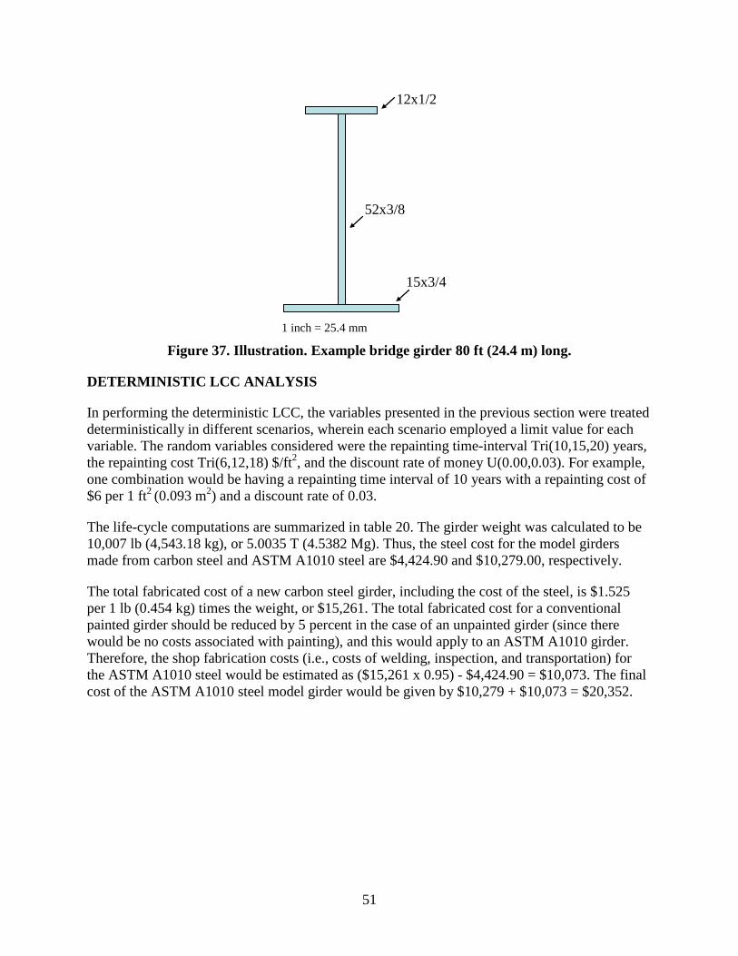
51

15x3/4

52x3/8

12x1/2

1 inch = 25.4 mm

Figure 37. Illustration. Example bridge girder 80 ft (24.4 m) long.

DETERMINISTIC LCC ANALYSIS

In performing the deterministic LCC, the variables presented in the previous section were treated deterministically in different scenarios, wherein each scenario employed a limit value for each variable. The random variables considered were the repainting time-interval Tri(10,15,20) years, the repainting cost Tri(6,12,18) $/ft2, and the discount rate of money U(0.00,0.03). For example, one combination would be having a repainting time interval of 10 years with a repainting cost of $6 per 1 ft2 (0.093 m2) and a discount rate of 0.03.

The life-cycle computations are summarized in table 20. The girder weight was calculated to be 10,007 lb (4,543.18 kg), or 5.0035 T (4.5382 Mg). Thus, the steel cost for the model girders made from carbon steel and ASTM A1010 steel are $4,424.90 and $10,279.00, respectively.

The total fabricated cost of a new carbon steel girder, including the cost of the steel, is $1.525 per 1 lb (0.454 kg) times the weight, or $15,261. The total fabricated cost for a conventional painted girder should be reduced by 5 percent in the case of an unpainted girder (since there would be no costs associated with painting), and this would apply to an ASTM A1010 girder. Therefore, the shop fabrication costs (i.e., costs of welding, inspection, and transportation) for the ASTM A1010 steel would be estimated as ($15,261 x 0.95) - $4,424.90 = $10,073. The final cost of the ASTM A1010 steel model girder would be given by $10,279 + $10,073 = $20,352.

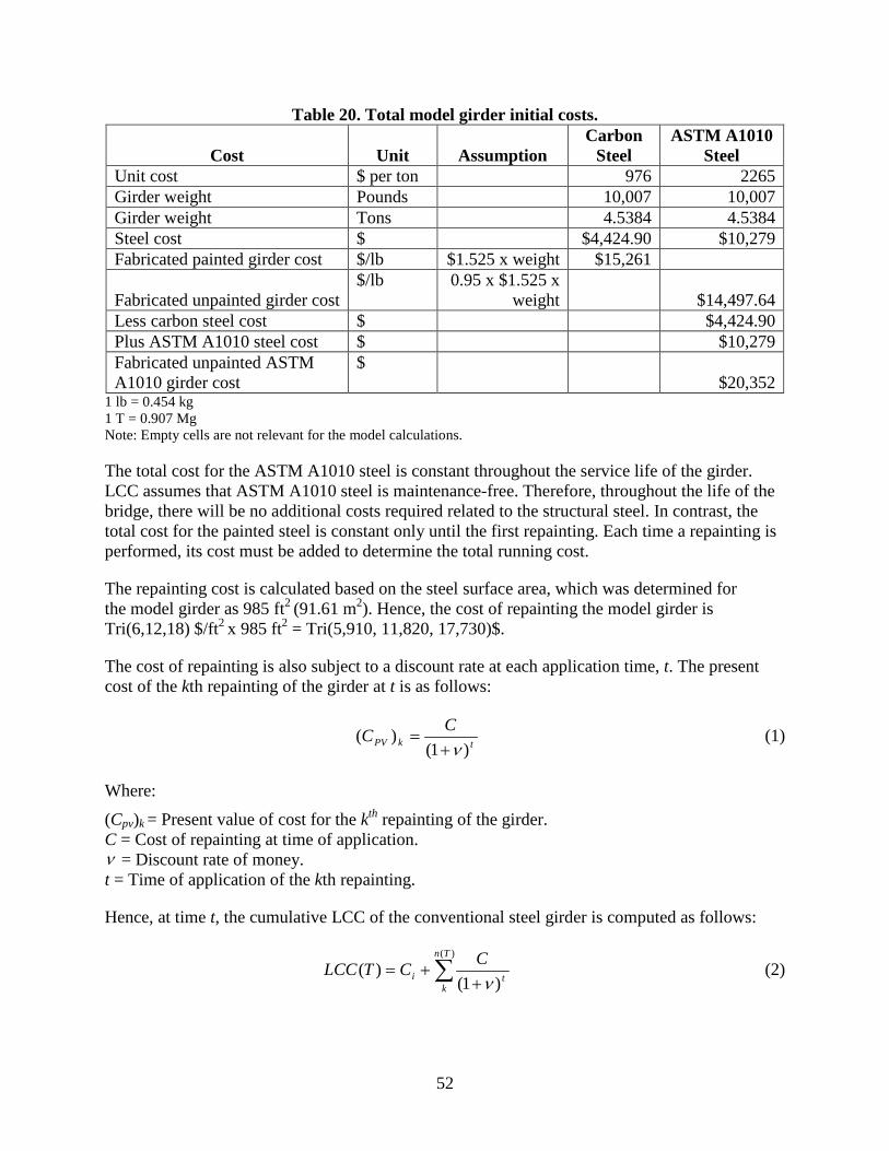
52

Table 20. Total model girder initial costs.

Cost Unit Assumption Carbon

Steel ASTM A1010

Steel Unit cost $ per ton 976 2265 Girder weight Pounds 10,007 10,007 Girder weight Tons 4.5384 4.5384 Steel cost $ $4,424.90 $10,279 Fabricated painted girder cost $/lb $1.525 x weight $15,261

Fabricated unpainted girder cost $/lb 0.95 x $1.525 x

weight $14,497.64 Less carbon steel cost $ $4,424.90 Plus ASTM A1010 steel cost $ $10,279 Fabricated unpainted ASTM A1010 girder cost

$ $20,352

1 lb = 0.454 kg 1 T = 0.907 Mg Note: Empty cells are not relevant for the model calculations.

The total cost for the ASTM A1010 steel is constant throughout the service life of the girder. LCC assumes that ASTM A1010 steel is maintenance-free. Therefore, throughout the life of the bridge, there will be no additional costs required related to the structural steel. In contrast, the total cost for the painted steel is constant only until the first repainting. Each time a repainting is performed, its cost must be added to determine the total running cost.

The repainting cost is calculated based on the steel surface area, which was determined for the model girder as 985 ft2 (91.61 m2). Hence, the cost of repainting the model girder is Tri(6,12,18) $/ft2 x 985 ft2 = Tri(5,910, 11,820, 17,730)$.

The cost of repainting is also subject to a discount rate at each application time, t. The present cost of the kth repainting of the girder at t is as follows:

tkPVCC

)1()(

ν+= (1)

Where:

(Cpv)k = Present value of cost for the kth repainting of the girder. C = Cost of repainting at time of application. ν = Discount rate of money. t = Time of application of the kth repainting.

Hence, at time t, the cumulative LCC of the conventional steel girder is computed as follows:

∑ ++=

)(

)1()(

Tn

kti

CCTLCCν

(2)

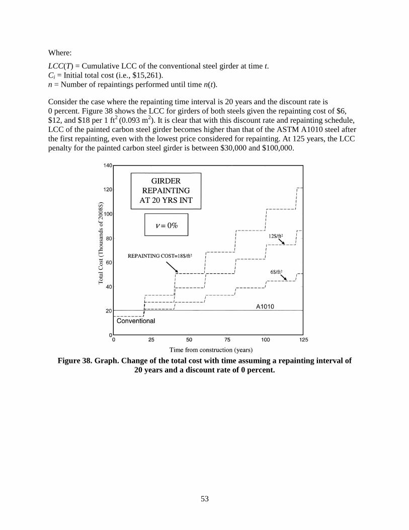
53

Where:

LCC(T) = Cumulative LCC of the conventional steel girder at time t. Ci = Initial total cost (i.e., $15,261). n = Number of repaintings performed until time n(t).

Consider the case where the repainting time interval is 20 years and the discount rate is 0 percent. Figure 38 shows the LCC for girders of both steels given the repainting cost of $6, $12, and $18 per 1 ft2 (0.093 m2). It is clear that with this discount rate and repainting schedule, LCC of the painted carbon steel girder becomes higher than that of the ASTM A1010 steel after the first repainting, even with the lowest price considered for repainting. At 125 years, the LCC penalty for the painted carbon steel girder is between $30,000 and $100,000.

Figure 38. Graph. Change of the total cost with time assuming a repainting interval of

20 years and a discount rate of 0 percent.

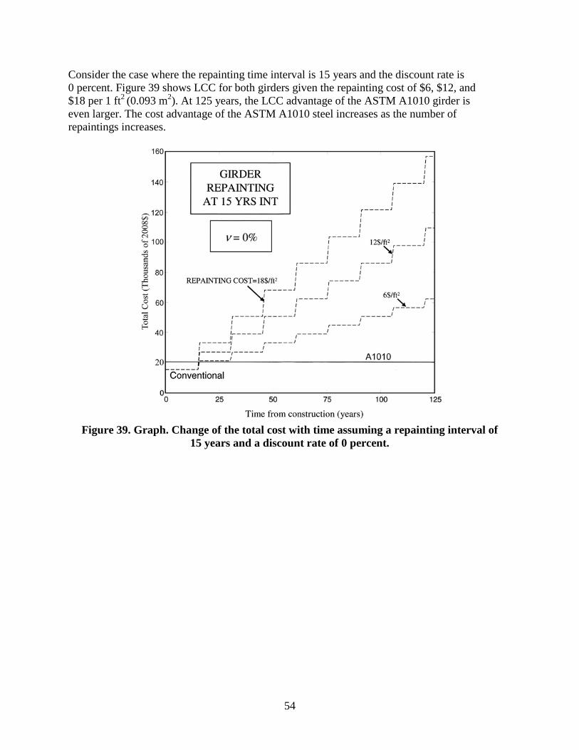
54

Consider the case where the repainting time interval is 15 years and the discount rate is 0 percent. Figure 39 shows LCC for both girders given the repainting cost of $6, $12, and $18 per 1 ft2 (0.093 m2). At 125 years, the LCC advantage of the ASTM A1010 girder is even larger. The cost advantage of the ASTM A1010 steel increases as the number of repaintings increases.

Figure 39. Graph. Change of the total cost with time assuming a repainting interval of

15 years and a discount rate of 0 percent.

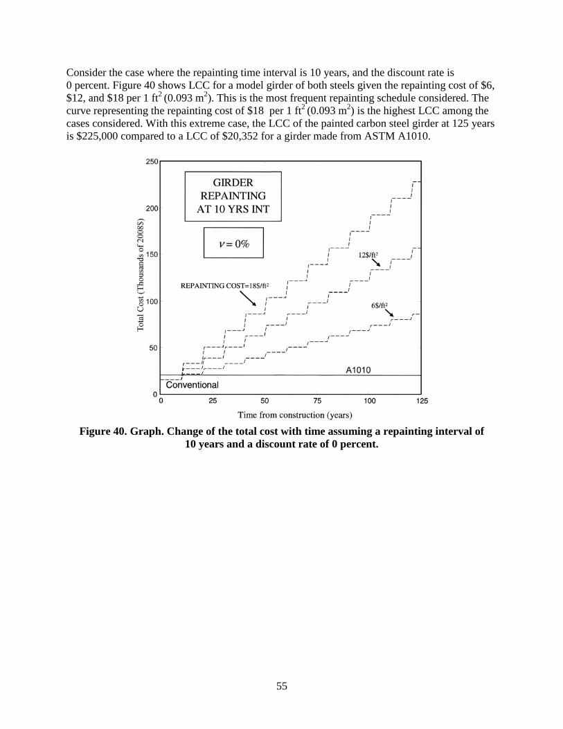
55

Consider the case where the repainting time interval is 10 years, and the discount rate is 0 percent. Figure 40 shows LCC for a model girder of both steels given the repainting cost of $6, $12, and $18 per 1 ft2 (0.093 m2). This is the most frequent repainting schedule considered. The curve representing the repainting cost of $18 per 1 ft2 (0.093 m2) is the highest LCC among the cases considered. With this extreme case, the LCC of the painted carbon steel girder at 125 years is $225,000 compared to a LCC of $20,352 for a girder made from ASTM A1010.

Figure 40. Graph. Change of the total cost with time assuming a repainting interval of

10 years and a discount rate of 0 percent.

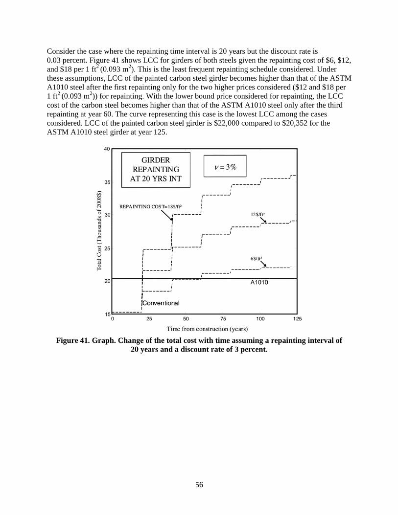
56

Consider the case where the repainting time interval is 20 years but the discount rate is 0.03 percent. Figure 41 shows LCC for girders of both steels given the repainting cost of $6, $12, and $18 per 1 ft2 (0.093 m2). This is the least frequent repainting schedule considered. Under these assumptions, LCC of the painted carbon steel girder becomes higher than that of the ASTM A1010 steel after the first repainting only for the two higher prices considered ($12 and $18 per 1 ft2 (0.093 m2)) for repainting. With the lower bound price considered for repainting, the LCC cost of the carbon steel becomes higher than that of the ASTM A1010 steel only after the third repainting at year 60. The curve representing this case is the lowest LCC among the cases considered. LCC of the painted carbon steel girder is $22,000 compared to $20,352 for the ASTM A1010 steel girder at year 125.

Figure 41. Graph. Change of the total cost with time assuming a repainting interval of

20 years and a discount rate of 3 percent.

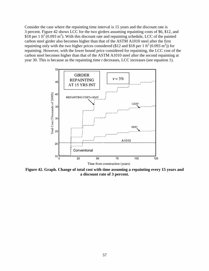
57

Consider the case where the repainting time interval is 15 years and the discount rate is 3 percent. Figure 42 shows LCC for the two girders assuming repainting costs of $6, $12, and $18 per 1 ft2 (0.093 m2). With this discount rate and repainting schedule, LCC of the painted carbon steel girder also becomes higher than that of the ASTM A1010 steel after the first repainting only with the two higher prices considered ($12 and $18 per 1 ft2 (0.093 m2)) for repainting. However, with the lower bound price considered for repainting, the LCC cost of the carbon steel becomes higher than that of the ASTM A1010 steel after the second repainting at year 30. This is because as the repainting time t decreases, LCC increases (see equation 1).

Figure 42. Graph. Change of total cost with time assuming a repainting every 15 years and

a discount rate of 3 percent.

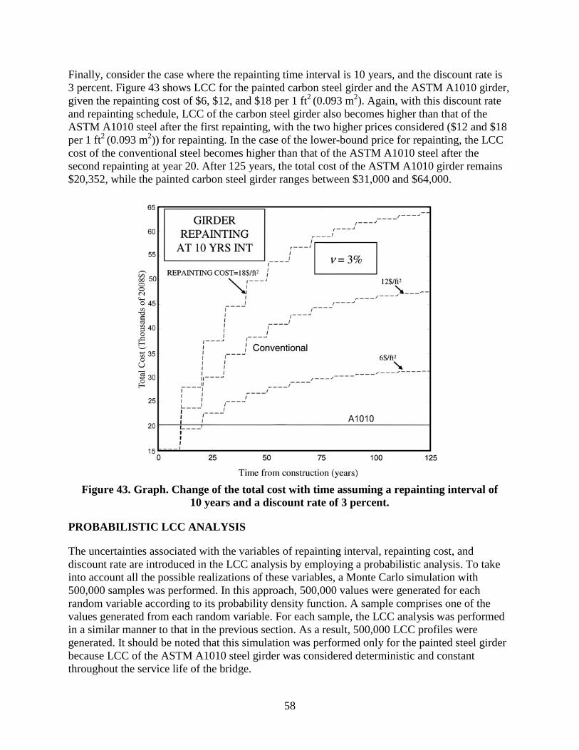
58

Finally, consider the case where the repainting time interval is 10 years, and the discount rate is 3 percent. Figure 43 shows LCC for the painted carbon steel girder and the ASTM A1010 girder, given the repainting cost of $6, $12, and $18 per 1 ft2 (0.093 m2). Again, with this discount rate and repainting schedule, LCC of the carbon steel girder also becomes higher than that of the ASTM A1010 steel after the first repainting, with the two higher prices considered ($12 and $18 per 1 ft2 (0.093 m2)) for repainting. In the case of the lower-bound price for repainting, the LCC cost of the conventional steel becomes higher than that of the ASTM A1010 steel after the second repainting at year 20. After 125 years, the total cost of the ASTM A1010 girder remains $20,352, while the painted carbon steel girder ranges between $31,000 and $64,000.

Figure 43. Graph. Change of the total cost with time assuming a repainting interval of

10 years and a discount rate of 3 percent.

PROBABILISTIC LCC ANALYSIS

The uncertainties associated with the variables of repainting interval, repainting cost, and discount rate are introduced in the LCC analysis by employing a probabilistic analysis. To take into account all the possible realizations of these variables, a Monte Carlo simulation with 500,000 samples was performed. In this approach, 500,000 values were generated for each random variable according to its probability density function. A sample comprises one of the values generated from each random variable. For each sample, the LCC analysis was performed in a similar manner to that in the previous section. As a result, 500,000 LCC profiles were generated. It should be noted that this simulation was performed only for the painted steel girder because LCC of the ASTM A1010 steel girder was considered deterministic and constant throughout the service life of the bridge.

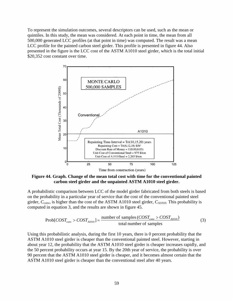
59

To represent the simulation outcomes, several descriptors can be used, such as the mean or quintiles. In this study, the mean was considered. At each point in time, the mean from all 500,000 generated LCC profiles (at that point in time) was computed. The result was a mean LCC profile for the painted carbon steel girder. This profile is presented in figure 44. Also presented in the figure is the LCC cost of the ASTM A1010 steel girder, which is the total initial $20,352 cost constant over time.

Figure 44. Graph. Change of the mean total cost with time for the conventional painted

carbon steel girder and the unpainted ASTM A1010 steel girder.

A probabilistic comparison between LCC of the model girder fabricated from both steels is based on the probability in a particular year of service that the cost of the conventional painted steel girder, Cconv, is higher than the cost of the ASTM A1010 steel girder, CA1010. This probability is computed in equation 3, and the results are shown in figure 45.

samples ofnumber total)( samples ofnumber ]Prob[ 1010

1010Aconv

AconvCOSTCOSTCOSTCOST >

=> (3)

Using this probabilistic analysis, during the first 10 years, there is 0 percent probability that the ASTM A1010 steel girder is cheaper than the conventional painted steel. However, starting in about year 12, the probability that the ASTM A1010 steel girder is cheaper increases rapidly, and the 50 percent probability occurs at year 15. By the 20th year of service, the probability is over 90 percent that the ASTM A1010 steel girder is cheaper, and it becomes almost certain that the ASTM A1010 steel girder is cheaper than the conventional steel after 40 years.

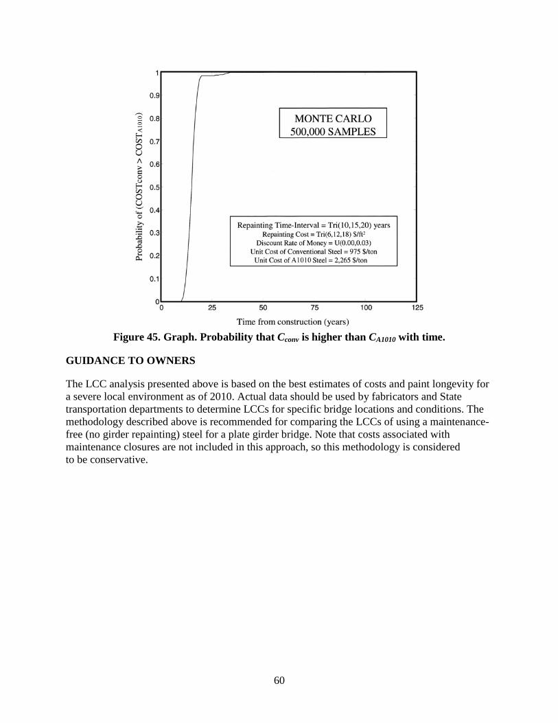
60

Figure 45. Graph. Probability that Cconv is higher than CA1010 with time.

GUIDANCE TO OWNERS

The LCC analysis presented above is based on the best estimates of costs and paint longevity for a severe local environment as of 2010. Actual data should be used by fabricators and State transportation departments to determine LCCs for specific bridge locations and conditions. The methodology described above is recommended for comparing the LCCs of using a maintenance-free (no girder repainting) steel for a plate girder bridge. Note that costs associated with maintenance closures are not included in this approach, so this methodology is considered to be conservative.

61

CHAPTER 8. CONCLUSIONS

• Of the high-Cr alloy steels studied in this investigation, only ASTM A1010 had the strength and toughness required to meet modern bridge steel design specifications.

• The corrosion behavior of the experimental steels in CCT is not a function of the steel YS.

• The laboratory CCTs demonstrated that reducing the Cr content from 11 percent typical of ASTM A1010 caused a significant reduction in corrosion resistance.

• As the Cr content of the experimental steels decreased from 11 to 5 percent, the corrosion rate (thickness loss) steadily increased.

• The effect of adding 2 percent Si to the 9 and 7 percent Cr steels was significantly detrimental to corrosion resistance.

• Substituting 2 percent Al for 2 percent Si in the 7 percent Cr steel had a positive effect on the corrosion rate.

• Under the conditions of the 5 and 3 percent NaCl CCTs in the laboratory, the corrosion rate of the ASTM A1010 steel was one-tenth to one-fifteenth that of ASTM A588.

• All the steels exhibited a relatively linear rate of thickness loss in the CCT, indicating that the corrosion products formed were not significantly protecting against continued corrosion.

• The corrosion products on the 11 percent Cr steels consisted of significantly less maghemite than the steels with lower Cr content. This is the apparent reason for the significantly better corrosion rates observed for the 11 percent Cr steels.

• The overall amount of goethite and lepidocrocite was equal for all the steels, so these corrosion products were not responsible for the significant difference in the CCT corrosion rates among the various steels.

• Atmospheric corrosion tests conducted on the Moore Drive Bridge with lower-Cr experimental steels containing 9 and 7 percent Cr exhibited between one-third and one-half the corrosion loss of ASTM A588 weathering steel. ASTM A1010 steel exposed on the Moore Drive Bridge had one-fourth the corrosion loss of ASTM A588, confirming that it was the most corrosion-resistant steel studied.

• After field exposure, the rust composition was similar for all three experimental steels. Akaganeite was the most abundant oxide and comprised about 70 percent of the rust. Goethite made up about 24 percent of the rust, and lepidocrocite made up about 6 percent. Notably absent was maghemite.

62

• The CCT protocol based on the SAE J2334 test is fundamentally different that actual field environments for bridges exposed to deicing salts because the high time-of-wetness of the CCT promotes the formation of maghemite.

• A 125-year LCC study of a model bridge girder made from ASTM A1010 steel versus a girder made from painted carbon steel showed ASTM A1010 to be the lower LCC material under all assumed conditions. After 15 years in service, the probability exceeds 50 percent that the ASTM A1010 steel is the lower cost material. After 40 years in service, it is certain that the ASTM A1010 steel is the lower cost material.

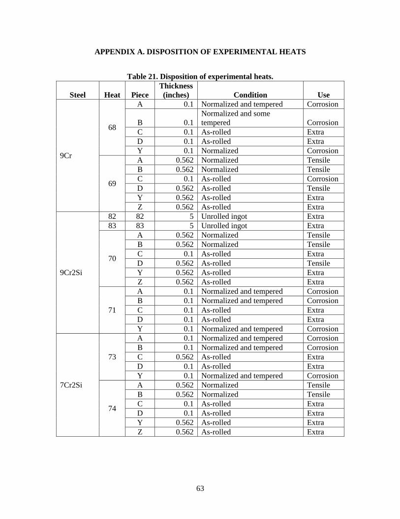
63

APPENDIX A. DISPOSITION OF EXPERIMENTAL HEATS

Table 21. Disposition of experimental heats.

Steel Heat Piece Thickness (inches) Condition Use

9Cr

68

A 0.1 Normalized and tempered Corrosion

B 0.1 Normalized and some tempered Corrosion

C 0.1 As-rolled Extra D 0.1 As-rolled Extra Y 0.1 Normalized Corrosion

69

A 0.562 Normalized Tensile B 0.562 Normalized Tensile C 0.1 As-rolled Corrosion D 0.562 As-rolled Tensile Y 0.562 As-rolled Extra Z 0.562 As-rolled Extra

9Cr2Si

82 82 5 Unrolled ingot Extra 83 83 5 Unrolled ingot Extra

70

A 0.562 Normalized Tensile B 0.562 Normalized Tensile C 0.1 As-rolled Extra D 0.562 As-rolled Tensile Y 0.562 As-rolled Extra Z 0.562 As-rolled Extra

71

A 0.1 Normalized and tempered Corrosion B 0.1 Normalized and tempered Corrosion C 0.1 As-rolled Extra D 0.1 As-rolled Extra Y 0.1 Normalized and tempered Corrosion

7Cr2Si

73

A 0.1 Normalized and tempered Corrosion B 0.1 Normalized and tempered Corrosion C 0.562 As-rolled Extra D 0.1 As-rolled Extra Y 0.1 Normalized and tempered Corrosion

74

A 0.562 Normalized Tensile B 0.562 Normalized Tensile C 0.1 As-rolled Extra D 0.1 As-rolled Extra Y 0.562 As-rolled Extra Z 0.562 As-rolled Extra

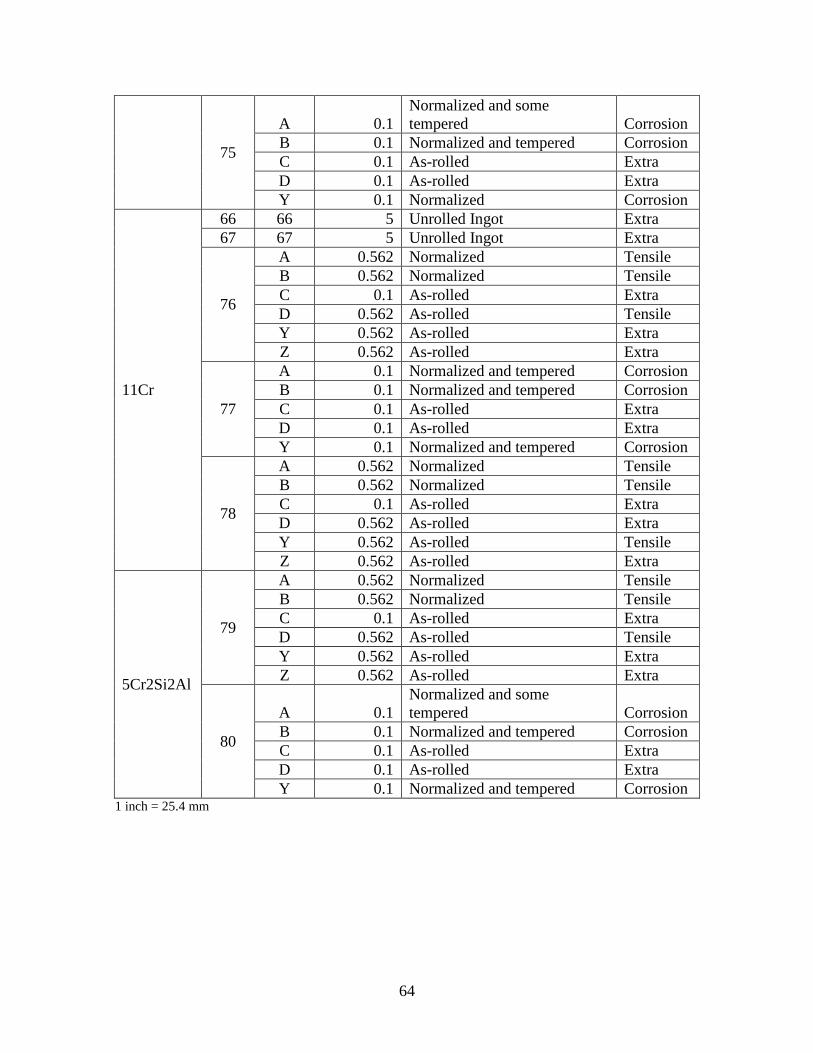
64

75

A 0.1 Normalized and some tempered Corrosion

B 0.1 Normalized and tempered Corrosion C 0.1 As-rolled Extra D 0.1 As-rolled Extra Y 0.1 Normalized Corrosion

11Cr

66 66 5 Unrolled Ingot Extra 67 67 5 Unrolled Ingot Extra

76

A 0.562 Normalized Tensile B 0.562 Normalized Tensile C 0.1 As-rolled Extra D 0.562 As-rolled Tensile Y 0.562 As-rolled Extra Z 0.562 As-rolled Extra

77

A 0.1 Normalized and tempered Corrosion B 0.1 Normalized and tempered Corrosion C 0.1 As-rolled Extra D 0.1 As-rolled Extra Y 0.1 Normalized and tempered Corrosion

78

A 0.562 Normalized Tensile B 0.562 Normalized Tensile C 0.1 As-rolled Extra D 0.562 As-rolled Extra Y 0.562 As-rolled Tensile Z 0.562 As-rolled Extra

5Cr2Si2Al

79

A 0.562 Normalized Tensile B 0.562 Normalized Tensile C 0.1 As-rolled Extra D 0.562 As-rolled Tensile Y 0.562 As-rolled Extra Z 0.562 As-rolled Extra

80

A 0.1 Normalized and some tempered Corrosion

B 0.1 Normalized and tempered Corrosion C 0.1 As-rolled Extra D 0.1 As-rolled Extra Y 0.1 Normalized and tempered Corrosion

1 inch = 25.4 mm

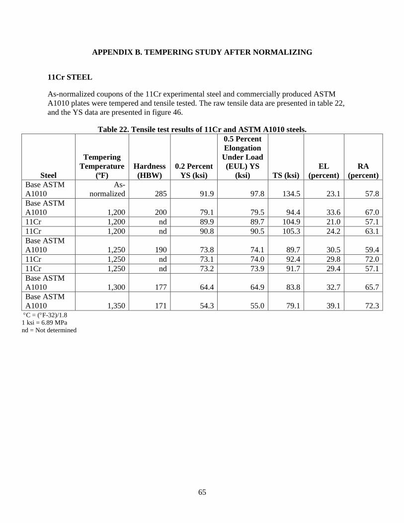
65

APPENDIX B. TEMPERING STUDY AFTER NORMALIZING

11Cr STEEL

As-normalized coupons of the 11Cr experimental steel and commercially produced ASTM A1010 plates were tempered and tensile tested. The raw tensile data are presented in table 22, and the YS data are presented in figure 46.

Table 22. Tensile test results of 11Cr and ASTM A1010 steels.

Steel

Tempering Temperature

(ºF) Hardness (HBW)

0.2 Percent YS (ksi)

0.5 Percent Elongation

Under Load (EUL) YS

(ksi) TS (ksi) EL

(percent) RA

(percent) Base ASTM A1010

As-normalized 285 91.9 97.8 134.5 23.1 57.8

Base ASTM A1010 1,200 200 79.1 79.5 94.4 33.6 67.0 11Cr 1,200 nd 89.9 89.7 104.9 21.0 57.1 11Cr 1,200 nd 90.8 90.5 105.3 24.2 63.1 Base ASTM A1010 1,250 190 73.8 74.1 89.7 30.5 59.4 11Cr 1,250 nd 73.1 74.0 92.4 29.8 72.0 11Cr 1,250 nd 73.2 73.9 91.7 29.4 57.1 Base ASTM A1010 1,300 177 64.4 64.9 83.8 32.7 65.7 Base ASTM A1010 1,350 171 54.3 55.0 79.1 39.1 72.3

°C = (°F-32)/1.8 1 ksi = 6.89 MPa nd = Not determined

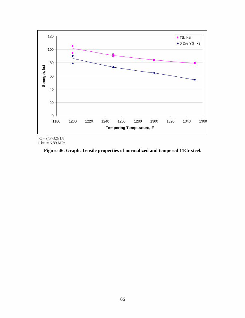
66

0

20

40

60

80

100

120

1180 1200 1220 1240 1260 1280 1300 1320 1340 1360

Tempering Temperature, F

Stre

ngth

, ksi

TS, ksi0.2% YS, ksi

°C = (°F-32)/1.8 1 ksi = 6.89 MPa

Figure 46. Graph. Tensile properties of normalized and tempered 11Cr steel.

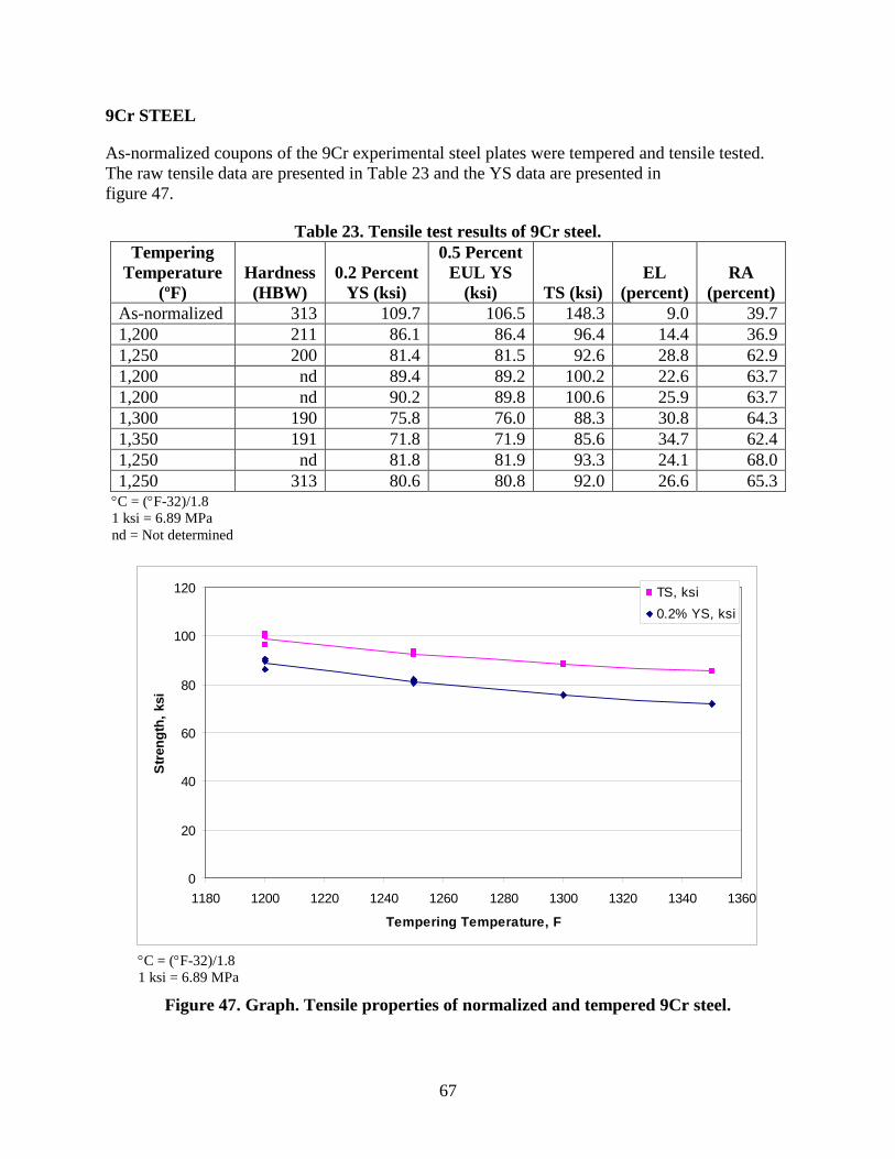
67

9Cr STEEL

As-normalized coupons of the 9Cr experimental steel plates were tempered and tensile tested. The raw tensile data are presented in Table 23 and the YS data are presented in figure 47.

Table 23. Tensile test results of 9Cr steel. Tempering

Temperature (ºF)

Hardness (HBW)

0.2 Percent YS (ksi)

0.5 Percent EUL YS

(ksi) TS (ksi) EL

(percent) RA

(percent) As-normalized 313 109.7 106.5 148.3 9.0 39.7 1,200 211 86.1 86.4 96.4 14.4 36.9 1,250 200 81.4 81.5 92.6 28.8 62.9 1,200 nd 89.4 89.2 100.2 22.6 63.7 1,200 nd 90.2 89.8 100.6 25.9 63.7 1,300 190 75.8 76.0 88.3 30.8 64.3 1,350 191 71.8 71.9 85.6 34.7 62.4 1,250 nd 81.8 81.9 93.3 24.1 68.0 1,250 313 80.6 80.8 92.0 26.6 65.3

°C = (°F-32)/1.8 1 ksi = 6.89 MPa nd = Not determined

0

20

40

60

80

100

120

1180 1200 1220 1240 1260 1280 1300 1320 1340 1360

Tempering Temperature, F

Stre

ngth

, ksi

TS, ksi0.2% YS, ksi

°C = (°F-32)/1.8 1 ksi = 6.89 MPa

Figure 47. Graph. Tensile properties of normalized and tempered 9Cr steel.

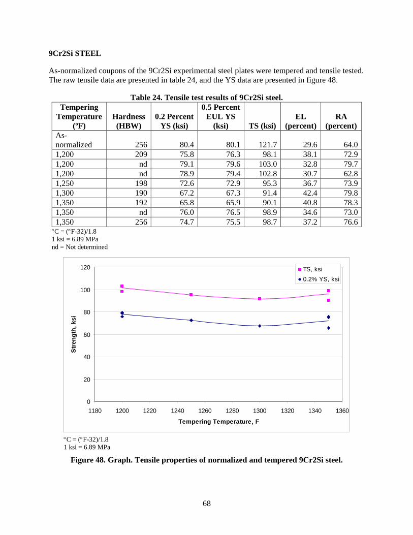
68

9Cr2Si STEEL

As-normalized coupons of the 9Cr2Si experimental steel plates were tempered and tensile tested. The raw tensile data are presented in table 24, and the YS data are presented in figure 48.

Table 24. Tensile test results of 9Cr2Si steel. Tempering

Temperature(ºF)

Hardness (HBW)

0.2 Percent YS (ksi)

0.5 Percent EUL YS

(ksi) TS (ksi) EL

(percent) RA

(percent) As-normalized 256 80.4 80.1 121.7 29.6 64.0 1,200 209 75.8 76.3 98.1 38.1 72.9 1,200 nd 79.1 79.6 103.0 32.8 79.7 1,200 nd 78.9 79.4 102.8 30.7 62.8 1,250 198 72.6 72.9 95.3 36.7 73.9 1,300 190 67.2 67.3 91.4 42.4 79.8 1,350 192 65.8 65.9 90.1 40.8 78.3 1,350 nd 76.0 76.5 98.9 34.6 73.0 1,350 256 74.7 75.5 98.7 37.2 76.6

°C = (°F-32)/1.8 1 ksi = 6.89 MPa nd = Not determined

0

20

40

60

80

100

120

1180 1200 1220 1240 1260 1280 1300 1320 1340 1360

Tempering Temperature, F

Stre

ngth

, ksi

TS, ksi0.2% YS, ksi

°C = (°F-32)/1.8 1 ksi = 6.89 MPa

Figure 48. Graph. Tensile properties of normalized and tempered 9Cr2Si steel.

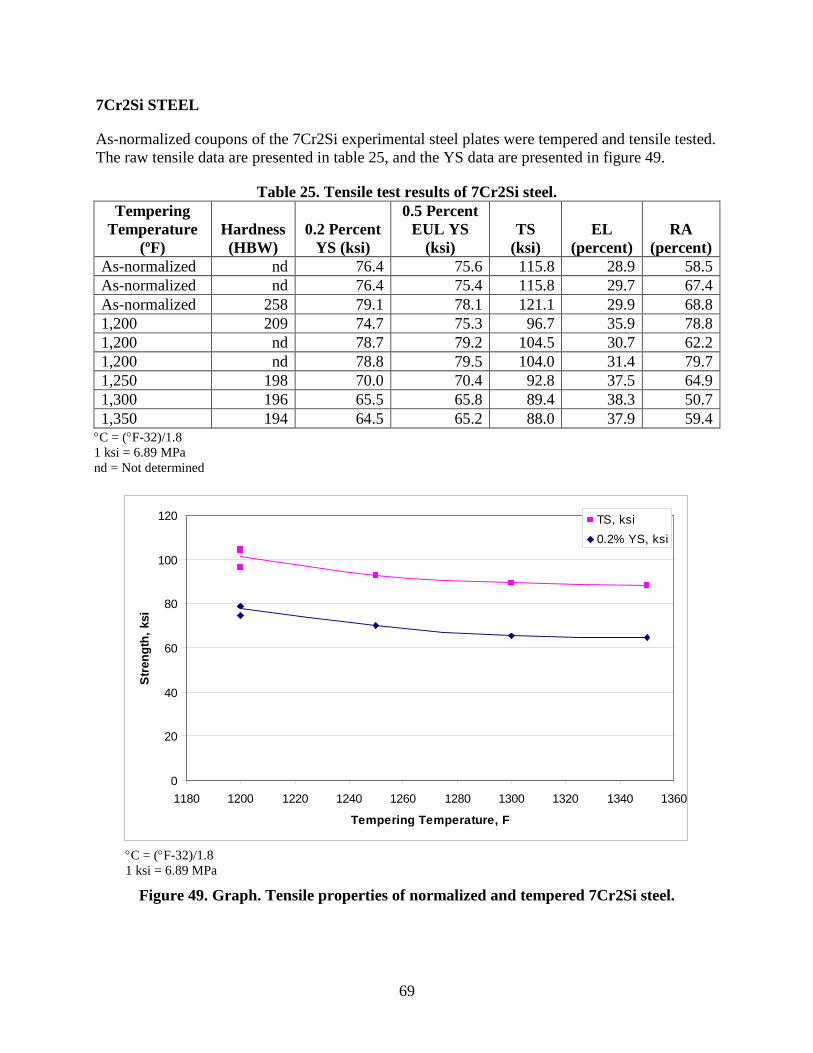
69

7Cr2Si STEEL

As-normalized coupons of the 7Cr2Si experimental steel plates were tempered and tensile tested. The raw tensile data are presented in table 25, and the YS data are presented in figure 49.

Table 25. Tensile test results of 7Cr2Si steel. Tempering

Temperature (ºF)

Hardness (HBW)

0.2 Percent YS (ksi)

0.5 Percent EUL YS

(ksi) TS

(ksi) EL

(percent) RA

(percent) As-normalized nd 76.4 75.6 115.8 28.9 58.5 As-normalized nd 76.4 75.4 115.8 29.7 67.4 As-normalized 258 79.1 78.1 121.1 29.9 68.8 1,200 209 74.7 75.3 96.7 35.9 78.8 1,200 nd 78.7 79.2 104.5 30.7 62.2 1,200 nd 78.8 79.5 104.0 31.4 79.7 1,250 198 70.0 70.4 92.8 37.5 64.9 1,300 196 65.5 65.8 89.4 38.3 50.7 1,350 194 64.5 65.2 88.0 37.9 59.4

°C = (°F-32)/1.8 1 ksi = 6.89 MPa nd = Not determined

0

20

40

60

80

100

120

1180 1200 1220 1240 1260 1280 1300 1320 1340 1360

Tempering Temperature, F

Stre

ngth

, ksi

TS, ksi0.2% YS, ksi

°C = (°F-32)/1.8 1 ksi = 6.89 MPa

Figure 49. Graph. Tensile properties of normalized and tempered 7Cr2Si steel.

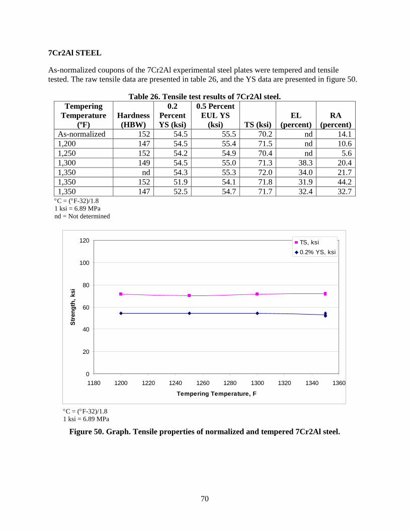
70

7Cr2Al STEEL

As-normalized coupons of the 7Cr2Al experimental steel plates were tempered and tensile tested. The raw tensile data are presented in table 26, and the YS data are presented in figure 50.

Table 26. Tensile test results of 7Cr2Al steel. Tempering

Temperature (ºF)

Hardness (HBW)

0.2 Percent YS (ksi)

0.5 Percent EUL YS

(ksi) TS (ksi) EL

(percent) RA

(percent) As-normalized 152 54.5 55.5 70.2 nd 14.1 1,200 147 54.5 55.4 71.5 nd 10.6 1,250 152 54.2 54.9 70.4 nd 5.6 1,300 149 54.5 55.0 71.3 38.3 20.4 1,350 nd 54.3 55.3 72.0 34.0 21.7 1,350 152 51.9 54.1 71.8 31.9 44.2 1,350 147 52.5 54.7 71.7 32.4 32.7

°C = (°F-32)/1.8 1 ksi = 6.89 MPa nd = Not determined

0

20

40

60

80

100

120

1180 1200 1220 1240 1260 1280 1300 1320 1340 1360

Tempering Temperature, F

Stre

ngth

, ksi

TS, ksi0.2% YS, ksi

°C = (°F-32)/1.8 1 ksi = 6.89 MPa

Figure 50. Graph. Tensile properties of normalized and tempered 7Cr2Al steel.

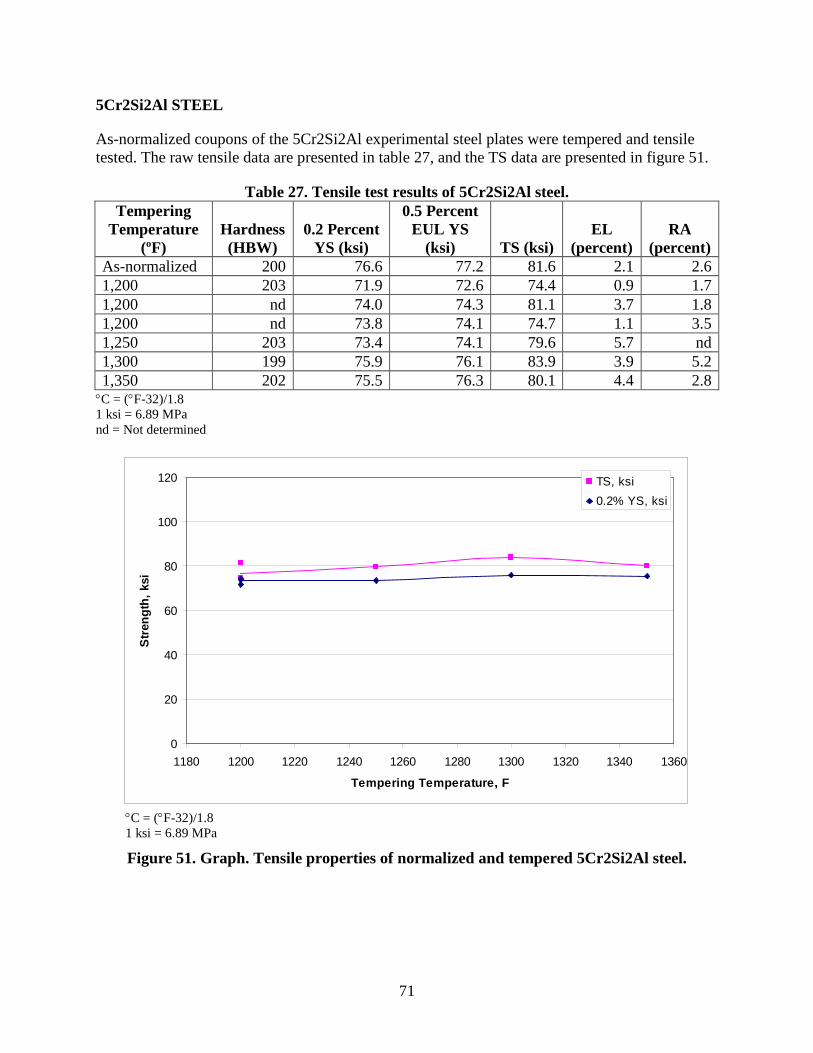
71

5Cr2Si2Al STEEL

As-normalized coupons of the 5Cr2Si2Al experimental steel plates were tempered and tensile tested. The raw tensile data are presented in table 27, and the TS data are presented in figure 51.

Table 27. Tensile test results of 5Cr2Si2Al steel. Tempering

Temperature (ºF)

Hardness (HBW)

0.2 Percent YS (ksi)

0.5 Percent EUL YS

(ksi) TS (ksi) EL

(percent) RA

(percent) As-normalized 200 76.6 77.2 81.6 2.1 2.6 1,200 203 71.9 72.6 74.4 0.9 1.7 1,200 nd 74.0 74.3 81.1 3.7 1.8 1,200 nd 73.8 74.1 74.7 1.1 3.5 1,250 203 73.4 74.1 79.6 5.7 nd 1,300 199 75.9 76.1 83.9 3.9 5.2 1,350 202 75.5 76.3 80.1 4.4 2.8

°C = (°F-32)/1.8 1 ksi = 6.89 MPa nd = Not determined

0

20

40

60

80

100

120

1180 1200 1220 1240 1260 1280 1300 1320 1340 1360

Tempering Temperature, F

Stre

ngth

, ksi

TS, ksi0.2% YS, ksi

°C = (°F-32)/1.8 1 ksi = 6.89 MPa

Figure 51. Graph. Tensile properties of normalized and tempered 5Cr2Si2Al steel.

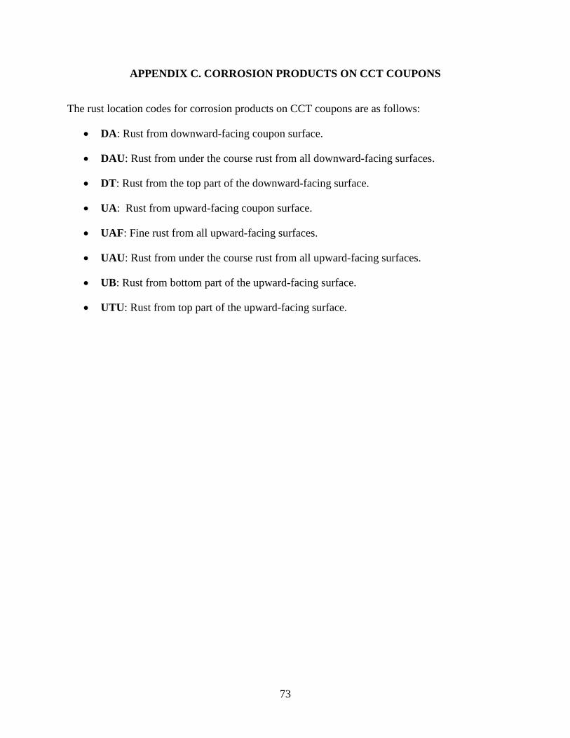
73

APPENDIX C. CORROSION PRODUCTS ON CCT COUPONS

The rust location codes for corrosion products on CCT coupons are as follows:

• DA: Rust from downward-facing coupon surface.

• DAU: Rust from under the course rust from all downward-facing surfaces.

• DT: Rust from the top part of the downward-facing surface.

• UA: Rust from upward-facing coupon surface.

• UAF: Fine rust from all upward-facing surfaces.

• UAU: Rust from under the course rust from all upward-facing surfaces.

• UB: Rust from bottom part of the upward-facing surface.

• UTU: Rust from top part of the upward-facing surface.

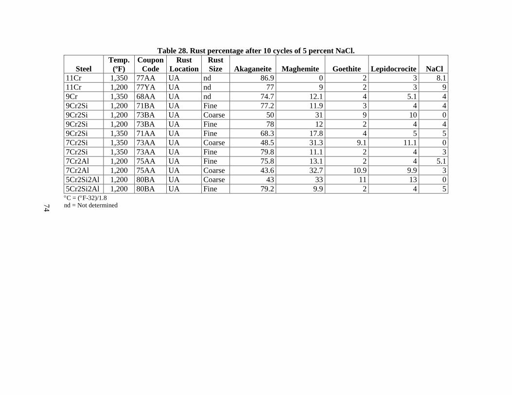
Table 28. Rust percentage after 10 cycles of 5 percent NaCl.

Steel Temp.

(ºF) Coupon

Code Rust

Location Rust Size Akaganeite Maghemite Goethite Lepidocrocite NaCl

11Cr 1,350 77AA UA nd 86.9 0 2 3 8.1 11Cr 1,200 77YA UA nd 77 9 2 3 9 9Cr 1,350 68AA UA nd 74.7 12.1 4 5.1 4 9Cr2Si 1,200 71BA UA Fine 77.2 11.9 3 4 4 9Cr2Si 1,200 73BA UA Coarse 50 31 9 10 0 9Cr2Si 1,200 73BA UA Fine 78 12 2 4 4 9Cr2Si 1,350 71AA UA Fine 68.3 17.8 4 5 5 7Cr2Si 1,350 73AA UA Coarse 48.5 31.3 9.1 11.1 0 7Cr2Si 1,350 73AA UA Fine 79.8 11.1 2 4 3 7Cr2Al 1,200 75AA UA Fine 75.8 13.1 2 4 5.1 7Cr2Al 1,200 75AA UA Coarse 43.6 32.7 10.9 9.9 3 5Cr2Si2Al 1,200 80BA UA Coarse 43 33 11 13 0 5Cr2Si2Al 1,200 80BA UA Fine 79.2 9.9 2 4 5

°C = (°F-32)/1.8 nd = Not determined

74

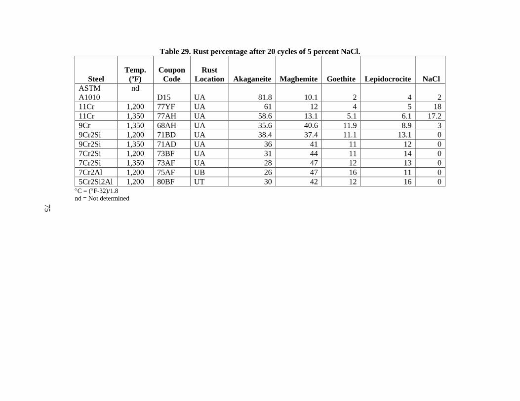
Table 29. Rust percentage after 20 cycles of 5 percent NaCl.

Steel

Temp.

(ºF)

Coupon

Code

Rust

Location

Akaganeite Maghemite Goethite Lepidocrocite

NaCl ASTM A1010

nd D15 UA 81.8 10.1 2 4 2

11Cr 1,200 77YF UA 61 12 4 5 18 11Cr 1,350 77AH UA 58.6 13.1 5.1 6.1 17.2 9Cr 1,350 68AH UA 35.6 40.6 11.9 8.9 3 9Cr2Si 1,200 71BD UA 38.4 37.4 11.1 13.1 0 9Cr2Si 1,350 71AD UA 36 41 11 12 0 7Cr2Si 1,200 73BF UA 31 44 11 14 0 7Cr2Si 1,350 73AF UA 28 47 12 13 0 7Cr2Al 1,200 75AF UB 26 47 16 11 0 5Cr2Si2Al 1,200 80BF UT 30 42 12 16 0

°C = (°F-32)/1.8 nd = Not determined 75

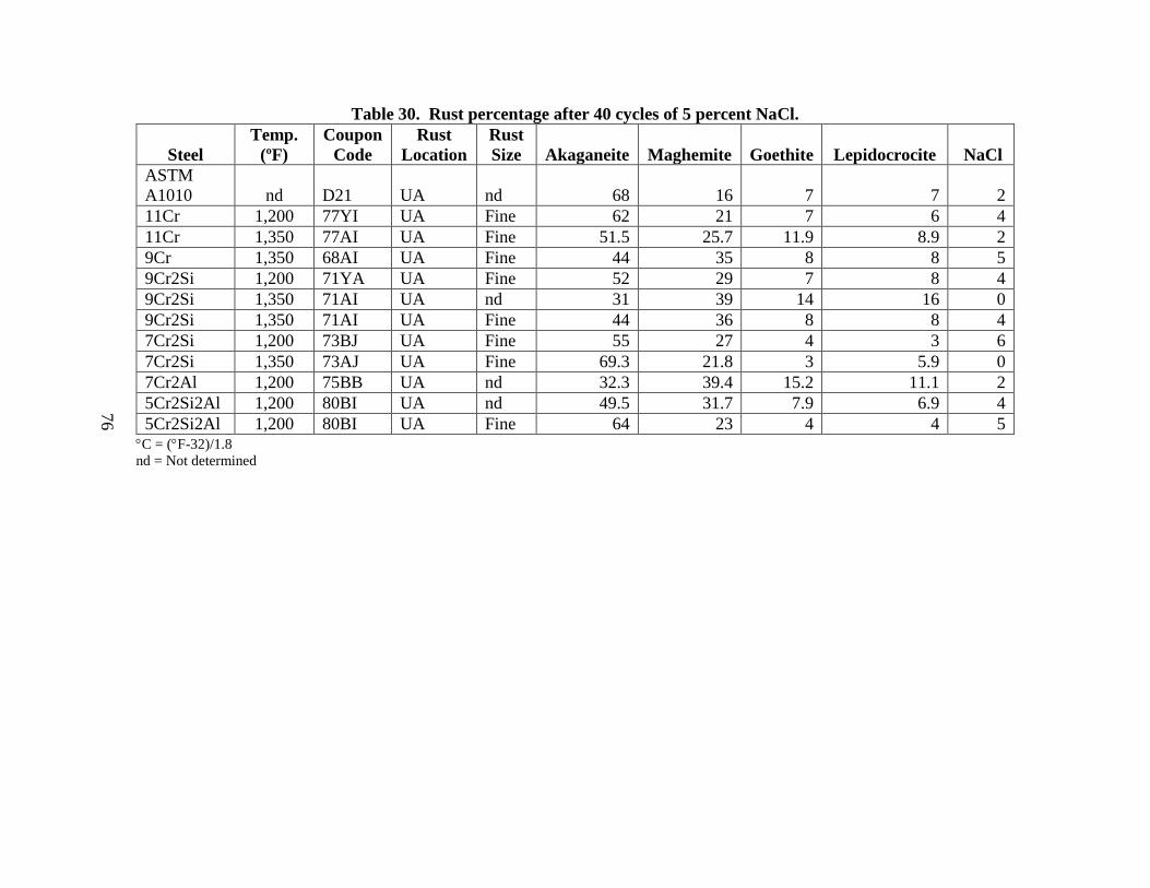
Table 30. Rust percentage after 40 cycles of 5 percent NaCl.

Steel Temp.

(ºF) Coupon

Code Rust

Location Rust Size Akaganeite Maghemite Goethite Lepidocrocite

NaCl

ASTM A1010 nd D21 UA nd 68 16 7 7 2 11Cr 1,200 77YI UA Fine 62 21 7 6 4 11Cr 1,350 77AI UA Fine 51.5 25.7 11.9 8.9 2 9Cr 1,350 68AI UA Fine 44 35 8 8 5 9Cr2Si 1,200 71YA UA Fine 52 29 7 8 4 9Cr2Si 1,350 71AI UA nd 31 39 14 16 0 9Cr2Si 1,350 71AI UA Fine 44 36 8 8 4 7Cr2Si 1,200 73BJ UA Fine 55 27 4 3 6 7Cr2Si 1,350 73AJ UA Fine 69.3 21.8 3 5.9 0 7Cr2Al 1,200 75BB UA nd 32.3 39.4 15.2 11.1 2 5Cr2Si2Al 1,200 80BI UA nd 49.5 31.7 7.9 6.9 4 5Cr2Si2Al 1,200 80BI UA Fine 64 23 4 4 5

°C = (°F-32)/1.8 nd = Not determined

76

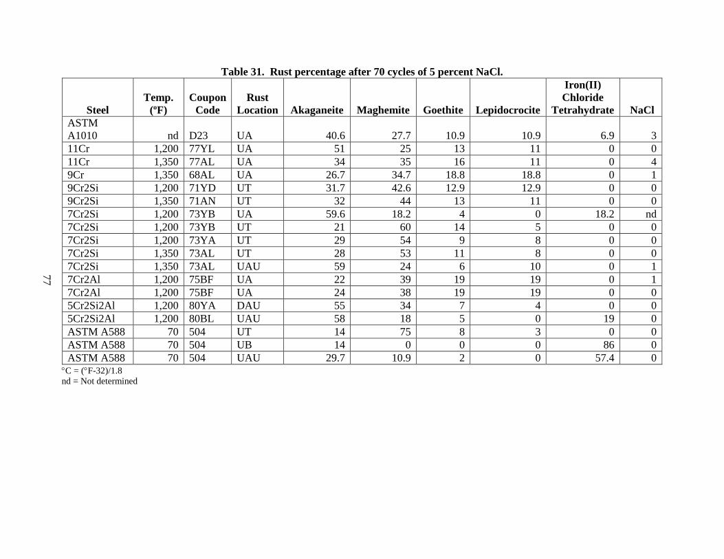
Table 31. Rust percentage after 70 cycles of 5 percent NaCl.

Steel Temp.

(ºF) Coupon

Code Rust

Location Akaganeite Maghemite Goethite Lepidocrocite

Iron(II) Chloride

Tetrahydrate

NaCl ASTM A1010 nd D23 UA 40.6 27.7 10.9 10.9 6.9 3 11Cr 1,200 77YL UA 51 25 13 11 0 0 11Cr 1,350 77AL UA 34 35 16 11 0 4 9Cr 1,350 68AL UA 26.7 34.7 18.8 18.8 0 1 9Cr2Si 1,200 71YD UT 31.7 42.6 12.9 12.9 0 0 9Cr2Si 1,350 71AN UT 32 44 13 11 0 0 7Cr2Si 1,200 73YB UA 59.6 18.2 4 0 18.2 nd 7Cr2Si 1,200 73YB UT 21 60 14 5 0 0 7Cr2Si 1,200 73YA UT 29 54 9 8 0 0 7Cr2Si 1,350 73AL UT 28 53 11 8 0 0 7Cr2Si 1,350 73AL UAU 59 24 6 10 0 1 7Cr2Al 1,200 75BF UA 22 39 19 19 0 1 7Cr2Al 1,200 75BF UA 24 38 19 19 0 0 5Cr2Si2Al 1,200 80YA DAU 55 34 7 4 0 0 5Cr2Si2Al 1,200 80BL UAU 58 18 5 0 19 0 ASTM A588 70 504 UT 14 75 8 3 0 0 ASTM A588 70 504 UB 14 0 0 0 86 0 ASTM A588 70 504 UAU 29.7 10.9 2 0 57.4 0

°C = (°F-32)/1.8 nd = Not determined

77

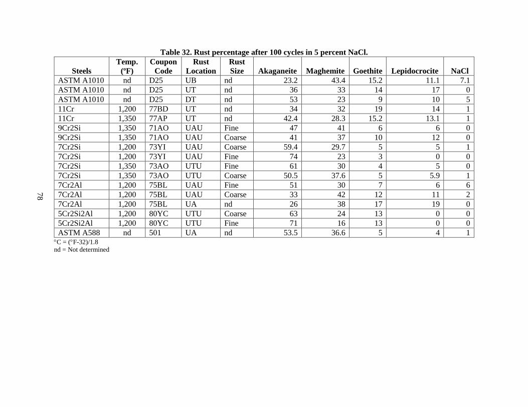
Table 32. Rust percentage after 100 cycles in 5 percent NaCl.

Steels Temp.

(ºF) Coupon

Code Rust

Location Rust Size Akaganeite Maghemite Goethite Lepidocrocite

NaCl

ASTM A1010 nd D25 UB nd 23.2 43.4 15.2 11.1 7.1 ASTM A1010 nd D25 UT nd 36 33 14 17 0 ASTM A1010 nd D25 DT nd 53 23 9 10 5 11Cr 1,200 77BD UT nd 34 32 19 14 1 11Cr 1,350 77AP UT nd 42.4 28.3 15.2 13.1 1 9Cr2Si 1,350 71AO UAU Fine 47 41 6 6 0 9Cr2Si 1,350 71AO UAU Coarse 41 37 10 12 0 7Cr2Si 1,200 73YI UAU Coarse 59.4 29.7 5 5 1 7Cr2Si 1,200 73YI UAU Fine 74 23 3 0 0 7Cr2Si 1,350 73AO UTU Fine 61 30 4 5 0 7Cr2Si 1,350 73AO UTU Coarse 50.5 37.6 5 5.9 1 7Cr2Al 1,200 75BL UAU Fine 51 30 7 6 6 7Cr2Al 1,200 75BL UAU Coarse 33 42 12 11 2 7Cr2Al 1,200 75BL UA nd 26 38 17 19 0 5Cr2Si2Al 1,200 80YC UTU Coarse 63 24 13 0 0 5Cr2Si2Al 1,200 80YC UTU Fine 71 16 13 0 0 ASTM A588 nd 501 UA nd 53.5 36.6 5 4 1

°C = (°F-32)/1.8 nd = Not determined

78

79

REFERENCES

1. ASTM A1010/A1010M. (2009). “Standard Specification for Higher-Strength Martensitic Stainless Steel Plate, Sheet, and Strip,” Annual Book of ASTM Standards, Volume 01.03, ASTM International, West Conshohocken, PA.

2. ASTM A709/A709M. (2010). “Standard Specification for Structural Steel for Bridges,” Annual Book of ASTM Standards, Volume 01.04, ASTM International, West Conshohocken, PA.

3. Federal Highway Administration. (1989). Uncoated Weathering Steel in Structures, Technical Advisory T4140.22, U.S. Department of Transportation, Washington, DC.

4. Fletcher, F.B. (2005). “Corrosion of Weathering Steels,” ASM Handbook 9A: Corrosion, ASM International, Materials Park, OH.

5. Cook, D.C., Oh, S.J., and Townsend, H.E. (1998). “The Protective Layer Formed on Steels after Long-Term Atmospheric Exposures,” Paper No. 343, Corrosion 98, NACE International, Houston, TX.

6. Fletcher, F.B., Townsend, H.E., and Wilson, A.D. (2003). Corrosion Performance of Improved Weathering Steels for Bridges, National Steel Bridge Alliance World Steel Bridge Symposium, Orlando, FL.

7. Fletcher, F.B. and Gagnepain, J.C. (2007). New Stainless Steels for Bridge Applications, International Bridge Conference, Pittsburgh, PA.

8. Duracorr®. (2008). Welding Guidelines, ArcelorMittal Technical Publication, Coatesville, PA.

9. ASTM G101–04. (2010). “Standard Guide for Estimating the Atmospheric Corrosion Resistance of Low-Alloy Steels,” Annual Book of ASTM Standards, Volume 03.02, ASTM International, West Conshohocken, PA.

10. ASTM A588/A588M-10. (2010). “Standard Specification for High-Strength Low-Alloy Structural Steel, up to 50 ksi [345 MPa] Minimum Yield Point, with Atmospheric Corrosion Resistance,” Annual Book of ASTM Standards, Volume 01.04, ASTM International, West Conshohocken, PA.

11. Cook, D.C. (2010). Moore Drive Bridge: Coupon Exposure Tests, AISI Corrosion Advisory Group Meeting, Washington, DC.

12. Baker, E.A. and Lee, T.S. (1982). “Calibration of Atmospheric Corrosion Test Sites,” Atmospheric Corrosion of Metals, ASTM STP 767, 250–266, ASTM International, West Conshohocken, PA.

13. SAE J2334. (1998). Lab Cosmetic Corrosion Test, SAE International, Warrendale, PA.

80

14. Townsend, H.E., Davidson, D.D., and Ostermiller, M.R. (1998). Development of Laboratory Corrosion Tests by the Automotive and Steel Industries of North America, 659–666, Proceedings of the Fourth International Conference on Zinc and Zinc-Alloy Coated Steel Sheet, Iron and Steel Institute of Japan, Tokyo, Japan.

15. Lula, R.A. (1986). Stainless Steel, ASM International, Materials Park, OH.

16. ASTM A370. (2010). “Standard Test Methods and Definitions for Mechanical Testing of Steel Products,” Annual Book of ASTM Standards, Volume 01.03, ASTM International, West Conshohocken, PA.

17. ASTM A36/A36M-08. (2010). “Standard Specification for Carbon Structural Steel,” Annual Book of ASTM Standards, Volume 01.04, ASTM International, West Conshohocken, PA.

18. ASTM G1-03. (2010). “Standard Practice for Preparing, Cleaning, and Evaluating Corrosion Test Specimens,” Annual Book of ASTM Standards, Volume 03.02, ASTM International, West Conshohocken, PA.

19. International Centre for Diffraction Data. ICDD®-PDF®-4 Database, Newtown Square, PA.

20. Cook, D.C. (2005). “Spectroscopic Identification of Protective and Non-Protective Corrosion Coatings on Steel Structures in Marine Environments,” Corrosion Science, 47, 2550–2570.

HRDI-60/11-11(WEB)E