


Languages
Pages
Legal


SYMBOL TIMING RECOVERY FOR CPM SIGNALS BASED ON MATCHED FILTERING
A THESIS SUBMITTED TO THE GRADUATE SCHOOL OF NATURAL AND APPLIED SCIENCES
OF MIDDLE EAST TECHNICAL UNIVERSITY
BY
ÇİLER BAŞERDEM
IN PARTIAL FULFILLMENT OF THE REQUIREMENTS FOR
THE DEGREE OF MASTER OF SCIENCE IN
THE DEPARTMENT OF ELECTRICAL AND ELECTRONICS ENGINEERING
DECEMBER 2006

Approval of the Graduate School of Natural and Applied Sciences
Prof. Dr. Canan Özgen Director
I certify that this thesis satisfies all the requirements as a thesis for the degree of Master of Science.
Prof. Dr. İsmet Erkmen Head of Department
This is to certify that we have read this thesis and that in our opinion it is fully adequate, in scope and quality, as a thesis for the degree of Master of Science.
Prof. Dr. Yalçın Tanık Supervisor Examining Committee Members Prof. Dr. Mete Severcan (METU, EE)
Prof. Dr. Yalçın Tanık (METU, EE)
Prof. Dr. Kerim Demirbaş (METU, EE)
Assist. Prof. Dr. Ali Özgür Yılmaz (METU, EE)
Çağdaş Enis Doyuran ( M.S.) (ASELSAN)

iii
I hereby declare that all information in this document has been obtained and presented in accordance with academic rules and ethical conduct. I also declare that, as required by these rules and conduct, I have fully cited and referenced all material and results that are not original to this work. Name, Last name : Çiler Başerdem
Signature :
iv
ABSTRACT
SYMBOL TIMING RECOVERY FOR CPM SIGNALS
BASED ON MATCHED FILTERING
Başerdem, Çiler
M.S., Department of Electrical and Electronics Engineering
Supervisor : Prof. Dr. Yalçın Tanık
December 2006, 96 pages
In this thesis, symbol timing recovery based on matched filtering in Gaussian
Minimum Shift Keying (GMSK) with bandwidth-bit period product (BT) of 0.3 is
investigated. GMSK is the standard modulation type for GSM. Although GMSK
modulation is non-linear, it is approximated to Offset Quadrature Amplitude
Modulation (OQAM), which is a linear modulation, so that Maximum Likelihood
Sequence Estimation (MLSE) method is possible in the receiver part. In this study
Typical Urban (TU) channel model developed in COST 207 is used. Two methods
are developed on the construction of the matched filter. In order to obtain timing
recovery for GMSK signals, these methods are investigated. The fractional time
delays are acquired by using interpolation and an iterative maximum search process.
The performance of the proposed symbol timing recovery (STR) scheme is assessed
by using computer simulations. It is observed that the STR tracks the variations of
the frequency selective multipath fading channels almost the same as the Mazo
criterion.

v
Keywords: Symbol timing recovery, Gaussian Minimum Shift Keying (GMSK),
matched filtering, multipath fading channel, Mazo criterion.
vi
ÖZ
CPM SİNYALLERİ İÇİN UYUMLU SÜZGEÇLEMEYE DAYALI SEMBOL ZAMAN BİLGİSİNİN KAZANIMI
Başerdem, Çiler
Yüksek Lisans, Elektrik ve Elektronik Mühendisliği Bölümü
Tez Yöneticisi : Prof. Dr. Yalçın Tanık
Aralık 2006, 96 sayfa
Bu tezde, bant genişliği ile bit aralığı çarpımı 0.3 olan Gaussian en küçük
kaydırmalı kiplenim (GMSK) sinyalleri için uyumlu süzgeçlemeye dayalı sembol
zaman bilgisinin kazanımı incelenmiştir. GMSK, GSM sistemi için standart
modülasyon tipidir. GMSK modülasyonu, doğrusal olmamasına rağmen, en büyük
olasılıklı dizi kestirimi (MLSE) yönteminin alıcı kısmında kullanılabilmesi için
doğrusal bir modülasyon tipi olan OQAM’ ye benzetilmiştir. Bu çalışmada COST
207 ‘de geliştirilen şehiriçi tipik kanal modeli kullanılmıştır. Uyumlu süzgeç yapısı
için iki yöntem geliştirilmiştir. GMSK sinyalleri için zaman bilgisinin kazanımını
elde etmek amacıyla bu iki yöntem incelenmiştir. Ufak zaman gecikmeleri,
aradeğerleme ve döngülü en yüksek arama yöntemleri kullanılarak elde edilmiştir.
Önerilen sembol zaman kazanım (STR) yapısının başarımı bilgisayar benzetimleri
kullanılarak değerlendirilmiştir. STR’nin frekans seçici çokyönlü sönümlemeli kanal
değişimlerini Mazo ölçütüne çok benzer takip ettiği gözlenmiştir.

vii
Anahtar kelimeler: Sembol zaman kazanımı, Gaussian en küçük kaydırmalı
kiplenim , uyumlu süzgeç, çokyönlü sönümlemeli kanal, Mazo ölçütü.

viii
To my family

ix
ACKNOWLEDGMENTS
I would like to express my appreciation to my supervisor Prof. Dr. Yalçın Tanık for
his supervision, support and helpful comments on this thesis.
I am also grateful to ASELSAN Inc. for letting and supporting of my thesis.
Additionally I would like to thank to Çağdaş Enis Doyuran for his motivative
comments and great contributions about writing this thesis.
I also wish to express my deep gratitude to my parents and my dear brother, for their
support during my life.
Finally, special thanks are due to my colleague Hazım Tokuçcu for his great support,
encouragement and patience throughout my thesis study.
x
TABLE OF CONTENTS
PLAGIARISM.............................................................................................................iii
ABSTRACT ........................................................................................................... iv
ÖZ .......................................................................................................................... vi
ACKNOWLEDGMENTS....................................................................................... ix
TABLE OF CONTENTS..........................................................................................x
LIST OF TABLES................................................................................................ xiii
LIST OF FIGURES ...............................................................................................xiv
LIST OF ABBREVATIONS................................................................................ xvii
CHAPTER.................................................................................................................
1. INTRODUCTION ..........................................................................................1
1.1 SCOPE AND OBJECTIVE........................................................................1
1.2 OUTLINE OF THE STUDY ......................................................................2
2. BACKGROUND MATERIAL........................................................................4
2.1 INTRODUCTION......................................................................................4
2.2 CHANNEL MODEL..................................................................................4
2.2.1 Characterization of Multipath Fading Channel ...................................5
2.2.2 Channel Statistical Characterization:..................................................6
2.2.2.1 Doppler Power Spectrum .............................................................6
xi
2.2.2.2 Delay Power Profile .....................................................................8
2.2.3 Generation of Tap-Gain Processes: ..................................................10
2.3 MLSE RECEIVER FOR THE GMSK SIGNAL.......................................13
2.3.1 The GMSK Signal ...........................................................................13
2.3.2 DEROTATION PROCEDURE .......................................................19
2.3.3. MLSE Receiver, Viterbi Algorithm and Channel Identification ......23
3. SYMBOL SYNCHRONIZATION REVIEW................................................28
3.1 INTRODUCTION....................................................................................28
3.2 SYMBOL TIMING RECOVERY ............................................................28
3.2.1 Existing STR Schemes.....................................................................30
3.2.2 Symbol Synchronization in CPM Signals.........................................33
3.3 MAXIMUM LIKELIHOOD TIMING ESTIMATION .............................34
4. A DD STR BASED ON MATCHED FILTERING FOR GMSK SIGNALS..39
4.1 INTRODUCTION....................................................................................39
4.2. CRITERIA FOR TIMING PHASE..........................................................40
4.2.1. Modified Cramer Rao Bound..........................................................40
4.2.2 Mazo Criterion ................................................................................42
4.3. PROPOSED DD STR FOR GMSK SIGNALS........................................46
4.3.1. Correlation (Matched Filter) Method ..............................................46
4.3.2. Iterative Maximum Search..............................................................49
4.3.3. Interpolation ...................................................................................50
4.3.4. Discussion on the Parameters..........................................................52
5. SIMULATION & RESULTS ........................................................................57
5.1 INTRODUCTION....................................................................................57
xii
5.2 SIMULATION MODEL OF THE COMMUNICATION SYSTEM .........57
5.2.1 GMSK Modulated Signal.................................................................59
5.2.2 Simulated Channel Specifications....................................................60
5.2.3 Methods on the Matched Filter ........................................................63
5.3 TRACKING PERFORMANCE OF THE PROPOSED SYMBOL SYNCHRONIZER ................................................................................70
5.3.1 Performance on the AWGN Channel ...............................................70
5.3.2 Performance on the Frequency Selective Fading Channel ................71
6. CONCLUSION.............................................................................................80
REFERENCES .......................................................................................................83
APPENDICES...........................................................................................................
A.CPM SIGNALS ..................................................................................................87
B.APPROXIMATION OF GMSK TO LINEAR QAM SIGNAL............................92

xiii
LIST OF TABLES
TABLES Table 2.1 Training sequence codes ………………………………………………… 24 Table 4.1 Normalized timing standard deviation for different interpolation length
and observation interval……..…………....................................................56 Table 4.2 Normalized timing standard deviation for Lo=32, Ni = 5…………….......56 Table 5.1 The rms error values for the simulations in Figure 5.9 and 5.10………....67 Table 5.2 The rms error values for the simulations in Figure 5.11 and 5.12……..…68 Table 5.3 The rms error values for the simulations in Figure 5.15
and 5.16…………………………………………….……………………..72 Table 5.4 The rms error values for the simulations in Figure 5.17………………….74 Table 5.5 The rms error values for the simulations in Figure 5.18……………….....74 Table 5.6 The rms error values for the simulations in Figure 5.19 and 5.20………..76 Table 5.7 The rms error values for the simulations in Figure 5.21…….…………....78 Table 5.8 The rms error values for the simulations in Figure 5.22………………….78
xiv
LIST OF FIGURES
FIGURES Figure 2.1 Multipath fading channel model……………………...…………………...5 Figure 2.2 Classical doppler spectrum ( df = 150 Hz)…………………………….....8
Figure 2.3 Power delay profile for Typical Urban (TU) channel……..……………...9 Figure 2.4 Filtering of white noise……………………………..……………………10 Figure 2.5 Adjustment of a tap weight………………………...…………………….11 Figure 2.6 Rayleigh fading envelope
df = 42 Hz………….……………..……….…12
Figure 2.7 Rayleigh fading envelope
df = 150 Hz…….…………………………….12
Figure 2.8 Baseband shaping pulse of g(t)…………………………….……………14 Figure 2.9 Generation of GMSK modulated signal………………….……………...15 Figure 2.10 Comparison of C0 (t) and C1 (t)………………………………………....17 Figure 2.11 Complex envelope of approximated GMSK signal …….……………...18 Figure 2.12 Power spectrum density of approximated and exact GMSK
signal……….…………………………………………………………..19 Figure 2.13 Correlation function between the central 16 bits and the whole
training sequence….……………..…………….………………………25 Figure 2.14 General block diagram of GMSK system model…………….………...27 Figure 3.1 Typical block diagram of a baseband receiver…………………………..29 Figure 3.2 Feedback configuration……………………………….………………....31
xv
Figure 3.3 Feedforward configuration…….………………………….……………..31 Figure 3.4 Synchronous sampling……………………….….…………………...….32 Figure 4.1 Error variance, ( )CRB τ and ( )MCRB τ ………………………………...41
Figure 4.2 Normalized timing phase obtained from Mazo criterion (v=50 km/h,
fc=900 MHz, fd = 42Hz)………………………………………………...45 Figure 4.3 Normalized timing phase obtained from Mazo criterion (v=90 km/h,
fc=1800 MHz, fd= 150Hz)…………………….………………………....45 Figure 4.4 General flow in the proposed timing recovery scheme…………………48 Figure 4.5 Illustration of the iteration process……………………………………...49 Figure 4.6 Impulse response of raised cosine filter………………………………....51 Figure 4.7 Illustration of k and τ in determining the timing instant……………….52 Figure 4.8 Normalized timing standard deviation for different SNR values………..54 Figure 4.9 Matched filter output with 0 32L = , SNR = 30 dB……………………...55
Figure 5.1 General block diagram of the simulated system………….………….….59 Figure 5.2 Complex envelope of the approximated GMSK signal……………....…60 Figure 5.3 Power spectrum density of linear GMSK and exact GMSK signal.….....60 Figure 5.4 Tapped delay line model of the multipath fading channel…….…….......61 Figure 5.5 Generation of taps……………………….…………………………...….62 Figure 5.6 Location of )(tsi
………………………………………………………...64
Figure 5.7 Construction of the reference signal by Method A…...……………....…65 Figure 5.8 Construction of the reference signal by Method B. ……...…...………...65 Figure 5.9 Comparison of the Methods A and B ( oL =16 , SNR=30dB,
v=50 km/h and fc= 900MHz )...…..…..…………………………….…...66 Figure 5.10 Comparison of the Methods A and B ( oL =32 , SNR=30dB,
v=50 km/h and fc= 900MHz )…...……….……………………………...67
xvi
Figure 5.11 Comparison of the Methods A and B ( oL =16 , SNR=30dB,
v=90 km/h and fc= 1800MHz )………...……………………….……….68 Figure 5.12 Comparison of the Methods A and B ( oL =32 , SNR=30dB,
v=90 km/h and fc= 1800MHz )…………….…………..…………….….69 Figure 5. 13 Performance of the symbol synchronizer for oL =16……………...…..70
Figure 5.14 Performance of the symbol synchronizer for oL =32…………………..71
Figure 5.15 Tracking performance of the proposed synchronizer for two
observation intervals (SNR=30dB, v=50 km/h and fc= 900MHz )...........73 Figure 5.16 Tracking performance of the proposed synchronizer for two
observation intervals (SNR=30dB, v=50 km/h and fc= 900MHz )……...73 Figure 5.17 Tracking performance of the proposed synchronizer for different roll
of factor values ( oL =32, SNR=30dB, v=50 km/h and fc= 900MHz )......75
Figure 5.18 Tracking performance of the proposed synchronizer for different SNR
values ( oL =32, v=50 km/h and fc= 900MHz )……………………….…75
Figure 5.19 Tracking performance of the proposed synchronizer for two observation
intervals (SNR=30dB, v=90 km/h and fc= 1800MHz )…………………77 Figure 5.20 Tracking performance of the proposed synchronizer for two observation
intervals (SNR=30dB, v=90 km/h and fc= 1800MHz )…………………77 Figure 5.21 Tracking performance of the proposed synchronizer for different roll
of factor values ( oL =32, SNR=30dB, v=90 km/h and fc= 1800MHz )…79
Figure 5.22 Tracking performance of the proposed synchronizer for different SNR
values ( oL =32, v=90 km/h and fc= 1800MHz )………………………...79
xvii
LIST OF ABBREVIATIONS
BT Bandwidth-Bit Period Product
BU Bad Urban
CIR Channel Impulse Response
CPM Continuous Phase Modulation
CRB Cramer Rao Bound
DA Data-aided
DD Decision-Directed
DECT Digital enhanced cordless telephone
GMSK Gaussian Minimum Shift Keying
GSM Global Systems Mobile Communications
HT Hilly Terrain
ISI Intersymbol Interference
LLF Log Likelihood Function
MCRB Modified Cramer Rao Bound
ML Maximum Likelihood
MLSE Maximum Likelihood Sequence Estimation
MMSE Minimum Mean Square Estimation
msISI Minimum Squared Intersymbol Interference
MSK Minimum Shift Keying
NCO Number Controlled Oscillator
xviii
NDA Non-Data Aided
NDD Non-Decision Directed
OQAM Offset Quadrature Amplitude Modulation
RA Rural Area
STR Symbol Timing Recovery
TED Timing Error Detector
TSC Training Sequence Code
TU Typical Urban
1
CHAPTER 1
INTRODUCTION
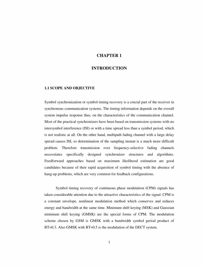
1.1 SCOPE AND OBJECTIVE
Symbol synchronization or symbol timing recovery is a crucial part of the receiver in
synchronous communication systems. The timing information depends on the overall
system impulse response thus, on the characteristics of the communication channel.
Most of the practical synchronizers have been based on transmission systems with no
intersymbol interference (ISI) or with a time spread less than a symbol period, which
is not realistic at all. On the other hand, multipath fading channel with a large delay
spread causes ISI, so determination of the sampling instant is a much more difficult
problem. Therefore transmission over frequency-selective fading channels
necessitates specifically designed synchronizer structures and algorithms.
Feedforward approaches based on maximum likelihood estimation are good
candidates because of their rapid acquisition of symbol timing with the absence of
hang-up problems, which are very common for feedback configurations.
Symbol timing recovery of continuous phase modulation (CPM) signals has
taken considerable attention due to the attractive characteristics of the signal. CPM is
a constant envelope, nonlinear modulation method which conserves and reduces
energy and bandwidth at the same time. Minimum shift keying (MSK) and Gaussian
minimum shift keying (GMSK) are the special forms of CPM. The modulation
scheme chosen by GSM is GMSK with a bandwidth symbol period product of
BT=0.3. Also GMSK with BT=0.5 is the modulation of the DECT system.

2
A timing recovery algorithm for MSK signals, which is able to extract the
fractional delays even in the presence of severe channel variation, is presented in [1].
The proposed method in [1] (and also in [2]) eliminates the cycle slips very
successfully. The recovery of the timing epoch is performed with matched filter
method, together with an interpolator and an iterative maximum search process. [1]
claims that the proposed recovery scheme is modulation independent and applicable
to any modulation type as CPM signals.
The objective of this thesis study is to examine symbol timing recovery for
GMSK which is one of the most popular modulation types of CPM signal used in
GSM. In this study, in order to investigate the performance of the proposed recovery
scheme (in [1] and [2]) in GMSK, two methods are developed on the construction of
the matched filter. Timing estimation for the GMSK is obtained by using one of
these methods and precise timing estimation is achieved by employing interpolation
and iterative maximum search process. Timing recovery scheme consists of two
modes. In acquisition mode, a data-aided approach is used for the adjustment of the
initial timing. Training sequence known by the receiver is used. In tracking mode,
tracking of the channel variation is performed with decision-directed timing
recovery, error free tentative decisions from MLSE receiver are assumed. Mazo
criterion is reviewed and used in order to assess the performance of the synchronizer.
1.2 OUTLINE OF THE STUDY
The thesis has the following outline:
In Chapter 2, the model of multipath fading channel, linear approximated
GMSK signal and the MLSE receiver structure are presented.
Basic timing recovery methods and maximum likelihood estimation of the
timing epoch are reviewed in Chapter 3.

3
In Chapter 4, important tools; modified Cramer-Rao bound and one of the
possible criteria; Mazo criteria are presented in order to assess performance of the
synchronizer. Then, the proposed timing recovery scheme, consisting of correlation
method, interpolation and the iterative maximum search algorithm in [1], is
reviewed. Finally, parameters which affect the performance of the timing recovery
scheme are discussed.
The simulations and results are presented in Chapter 5. The simulated system
is described in detail. Methods developed on construction of the matched filter are
discussed which are special for GMSK application. Tracking ability of the proposed
timing scheme for GMSK is presented through the simulation results.
In the last chapter, conclusions and possible future work are presented.
The general form of the CPM signals and especially MSK and GMSK signals
are given in Appendix A.
In Appendix B, approximation of GMSK signal to linear QAM signal is
presented in detail.
4
CHAPTER 2
BACKGROUND MATERIAL
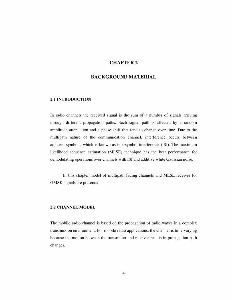
2.1 INTRODUCTION
In radio channels the received signal is the sum of a number of signals arriving
through different propagation paths. Each signal path is affected by a random
amplitude attenuation and a phase shift that tend to change over time. Due to the
multipath nature of the communication channel, interference occurs between
adjacent symbols, which is known as intersymbol interference (ISI). The maximum
likelihood sequence estimation (MLSE) technique has the best performance for
demodulating operations over channels with ISI and additive white Gaussian noise.
In this chapter model of multipath fading channels and MLSE receiver for
GMSK signals are presented.
2.2 CHANNEL MODEL
The mobile radio channel is based on the propagation of radio waves in a complex
transmission environment. For mobile radio applications, the channel is time-varying
because the motion between the transmitter and receiver results in propagation path
changes.
5
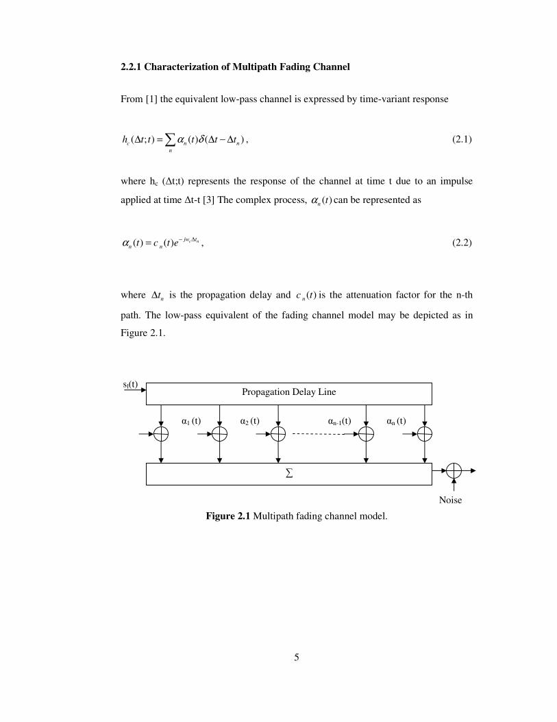
2.2.1 Characterization of Multipath Fading Channel
From [1] the equivalent low-pass channel is expressed by time-variant response
( ; ) ( ) ( )c n n
n
h t t t t tα δ∆ = ∆ − ∆∑ , (2.1)
where hc (∆t;t) represents the response of the channel at time t due to an impulse
applied at time ∆t-t [3] The complex process, ( )n tα can be represented as
( ) ( ) c njw t
n nt c t eα − ∆= , (2.2)
where nt∆ is the propagation delay and ( )nc t is the attenuation factor for the n-th
path. The low-pass equivalent of the fading channel model may be depicted as in
Figure 2.1.
Figure 2.1 Multipath fading channel model.
∑
α1 (t) α2 (t) αn-1(t) αn (t)
sl(t)
Noise
Propagation Delay Line
6
2.2.2 Channel Statistical Characterization:
The scattering function S(∆t;f) is the most important statistical measure of the
random multipath channel. It is a function of two variables; ∆t (delay) and a
frequency domain variable f is called the Doppler frequency. The scattering function
provides a single measure of the average power output of the channel as a function of
the delay ∆t and the f Doppler frequency. In other words, the scattering function
describes the manner in which the transmitted power is distributed in time and
frequency, upon passing through the channel. From the scattering function we can
obtain some of the most important relationships of a channel which impact the
performance of a communication system operating over that channel.
The delay-power profile P (∆t), which is also referred to as the multipath
intensity profile, is related to the scattering function via
( ) ( , )P t S t f df
∞
−∞
∆ = ∆∫ . (2.3)
Another function that is useful in characterizing fading is the Doppler power
spectrum, which is derived from the scattering function through
( ) ( , )S f S t f d t
∞
−∞
= ∆ ∆∫ . (2.4)
Different propagation models can be described by defining discrete number
of taps, each determined by their time delay and average power.
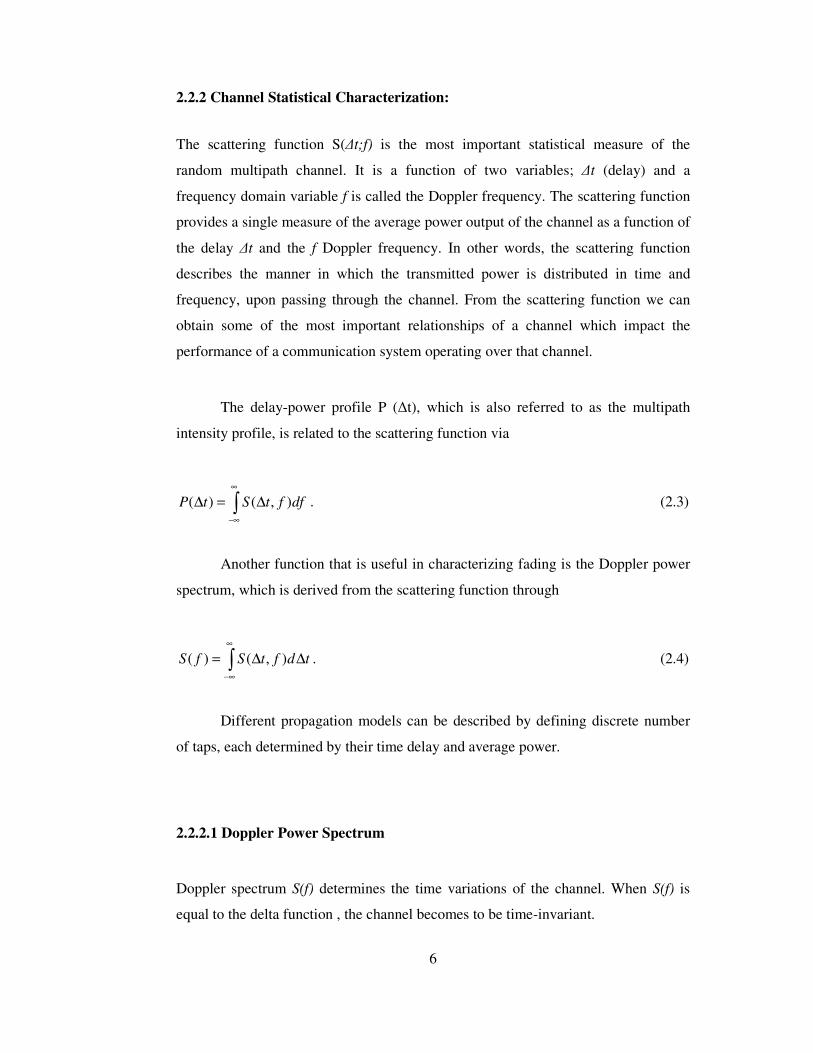
2.2.2.1 Doppler Power Spectrum
Doppler spectrum S(f) determines the time variations of the channel. When S(f) is
equal to the delta function , the channel becomes to be time-invariant.

7
For modeling of the channel, three types of Doppler spectra is defined in
COST 207 final report; classical Doppler spectrum, Gauss 1 and Gauss 2 [4]. The
most commonly used, and in a certain sense, the worst case Doppler spectrum is the
classical Doppler spectrum which is also called Jakes spectrum. In this spectrum
type, all the angle between vehicle speed and radio wave are assumed to be equally
probable [5]. The classical Doppler spectrum
1/ 22( ) for (- , )
1 ( / )d d
d
AS f f f f
f f= ∈ −
, (2.5)
where fd is maximum Doppler shift, and
d c
vf f
c= ⋅ , (2.6)
where v is the velocity of the mobile and cf the carrier frequency. The classical
Doppler spectrum is used throughout this study.
Classical Doppler spectrum for a mobile speed of 90 km/h and a carrier
frequency of 1800 MHz is shown in Figure 2.2.
8
Figure 2.2 Classical doppler spectrum ( df = 150 Hz).
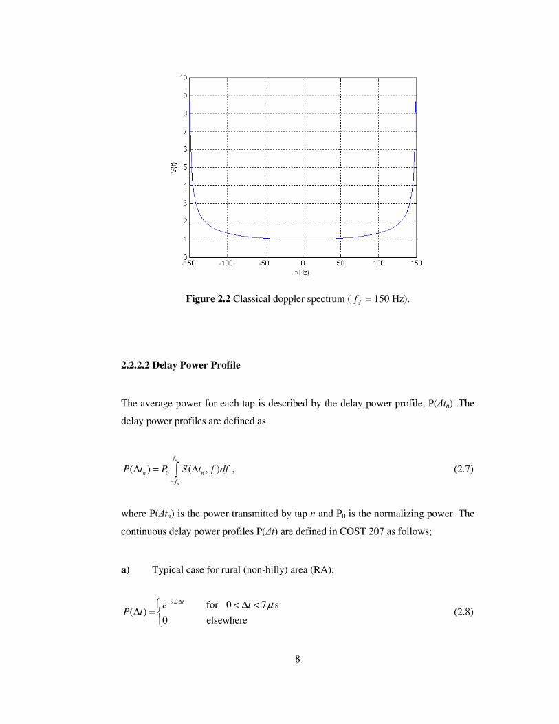
2.2.2.2 Delay Power Profile
The average power for each tap is described by the delay power profile, P(∆tn) .The
delay power profiles are defined as
0( ) ( , )d
d
f
n n
f
P t P S t f df−
∆ = ∆∫ , (2.7)
where P(∆tn) is the power transmitted by tap n and P0 is the normalizing power. The
continuous delay power profiles P(∆t) are defined in COST 207 as follows;
a) Typical case for rural (non-hilly) area (RA);
9.2 for 0 7 s( )
0 elsewhere
te tP t
µ− ∆ < ∆ <∆ =
(2.8)
9
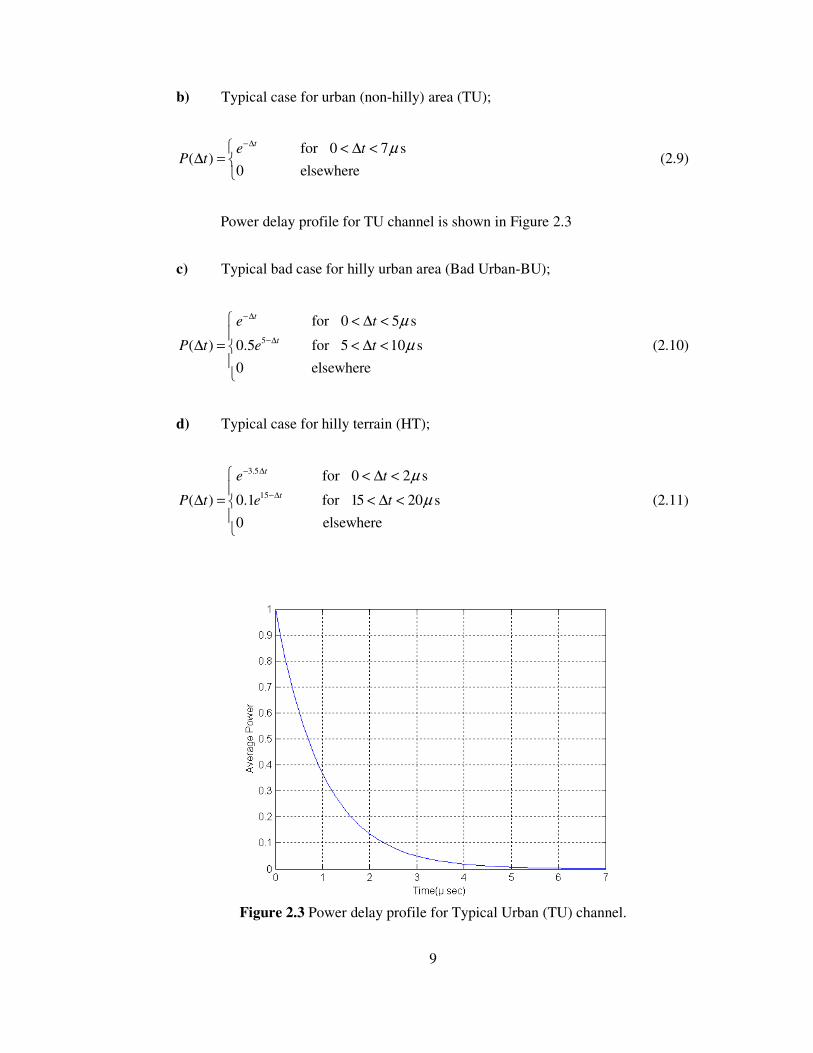
b) Typical case for urban (non-hilly) area (TU);
for 0 7 s( )
0 elsewhere
te tP t
µ−∆ < ∆ <∆ =
(2.9)
Power delay profile for TU channel is shown in Figure 2.3
c) Typical bad case for hilly urban area (Bad Urban-BU);
5
for 0 5 s
( ) 0.5 for 5 10 s
0 elsewhere
t
t
e t
P t e t
µ
µ
−∆
−∆
< ∆ <
∆ = < ∆ <
(2.10)
d) Typical case for hilly terrain (HT);
3.5
15
for 0 2 s
( ) 0.1 for 15 20 s
0 elsewhere
t
t
e t
P t e t
µ
µ
− ∆
−∆
< ∆ <
∆ = < ∆ <
(2.11)
Figure 2.3 Power delay profile for Typical Urban (TU) channel.

10
2.2.3 Generation of Tap-Gain Processes:
In order to obtain the tap gain, it is sufficient to generate a signal whose frequency
response is the scattering function. This can be accomplished by properly filtering
white noise as shown in Figure 2.4. The flatness of the frequency spectrum of the
filtering white noise results in simplification on the design of the shaping filter.
Figure 2.4 Filtering of white noise.
2( ) ( ) ( )wS f H f S f= . (2.12)
Sw(f) is the power spectral density of the white noise. Since the power spectral
density of the white noise is a constant for all frequencies, the magnitude of the
shaping filter response H(f) becomes
( ) ( )H f S f= . (2.13)
1 2
1 42( )
1 ( )d
AH f
f f= −
. (2.14)
h(t)= A1/2 2.583 fd x
-1/4 J1/4(x), (2.15)
where J1/4(.) is the fractional Bessel function and x=2π fd |t|. The shaping filter gain
A1/2 is chosen such that h(t) has the normalized power of 1.
H(f) White Noise S(f)
11
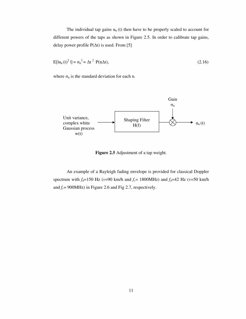
The individual tap gains αn (t) then have to be properly scaled to account for
different powers of the taps as shown in Figure 2.5. In order to calibrate tap gains,
delay power profile P(∆t) is used. From [5]
E[|αn (t)2 |] = σn
2 = ∆t 2 P(n∆t), (2.16)
where σn is the standard deviation for each n.
Figure 2.5 Adjustment of a tap weight.
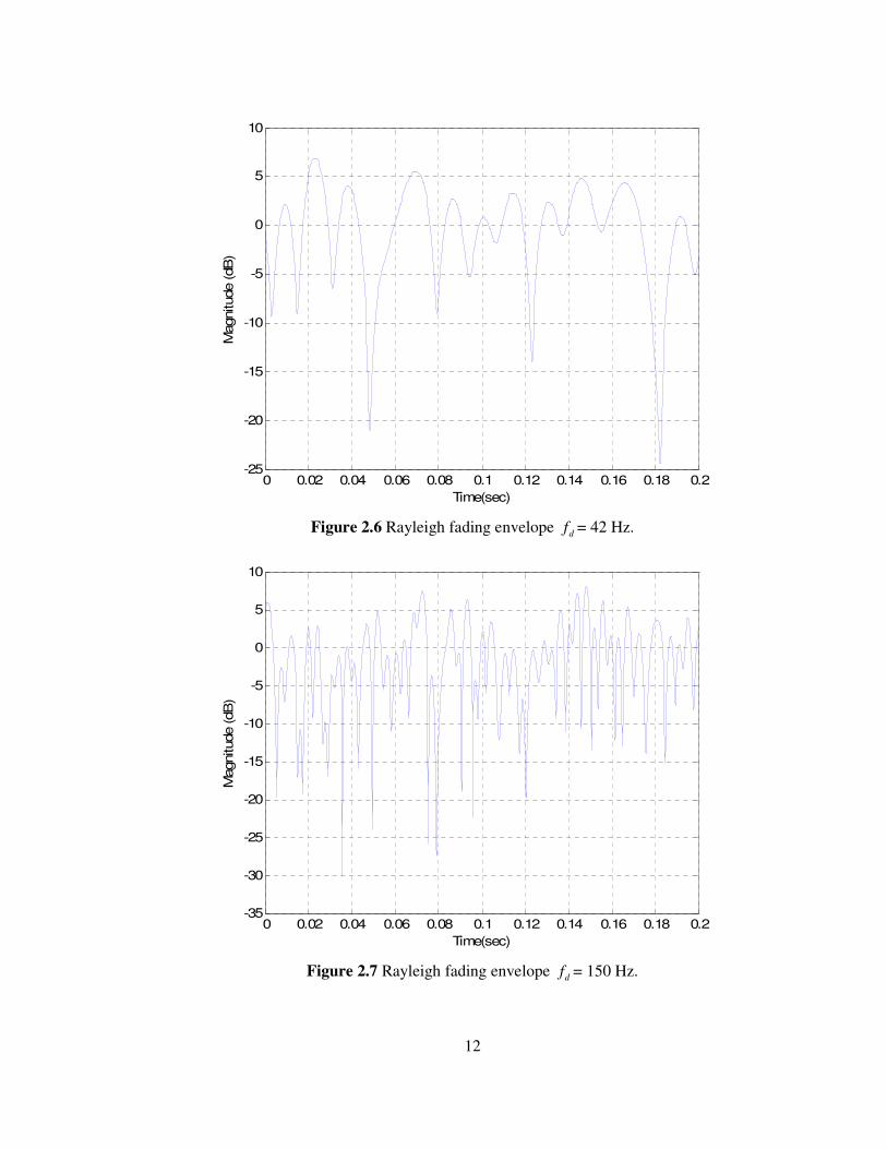
An example of a Rayleigh fading envelope is provided for classical Doppler
spectrum with fd=150 Hz (v=90 km/h and fc= 1800MHz) and fd=42 Hz (v=50 km/h
and fc= 900MHz) in Figure 2.6 and Fig 2.7, respectively.
Gain σn
Unit variance, complex white Gaussian process
w(t)
Shaping Filter H(f) αn (t)
12
0 0.02 0.04 0.06 0.08 0.1 0.12 0.14 0.16 0.18 0.2-25
-20
-15
-10
-5
0
5
10
Time(sec)
Magnitude (dB
)
Figure 2.6 Rayleigh fading envelope df = 42 Hz.
0 0.02 0.04 0.06 0.08 0.1 0.12 0.14 0.16 0.18 0.2-35
-30
-25
-20
-15
-10
-5
0
5
10
Time(sec)
Magnitude (dB
)
Figure 2.7 Rayleigh fading envelope df = 150 Hz.
13
2.3 MLSE RECEIVER FOR THE GMSK SIGNAL
2.3.1 The GMSK Signal
GMSK belongs to a family of the general class of continuous-phase modulation (i.e,
binary CPM with h=0.5) (see Appendix A CPM Signals), which has special
advantages of being quite narrow in its band with low adjacent channel interference
and a constant amplitude envelope which allows the use of efficient amplifiers in the
transmitters without special linearity requirements (class C amplifiers). Such
amplifiers are especially inexpensive to manufacture and have high degree of
efficiency [6].
As shown in Appendix A, the complex envelope of a GMSK signal is
));((2)( ταφθ −+= tis e
T
Ets . (2.17)
The phase of the modulated signal is:
( ; ) 2 ( )i
i
t h q t iφ α π α τ= −∑ , (2.18)
where the modulating index h is 0.5 and q(t) is the phase pulse of the
modulator. Relation between q(t) and g(t) is given in (A.3). g(t) is the baseband
shaping function given in (A.10) as
1 2 ( / 2) 2 ( / 2)( )
2 ln 2 ln 2
B t T B t Tg t erf erf
T
π π − += − + −
. (2.19)
In the equation above, B is the 3 dB bandwidth of the filter and T is the bit
duration.
14
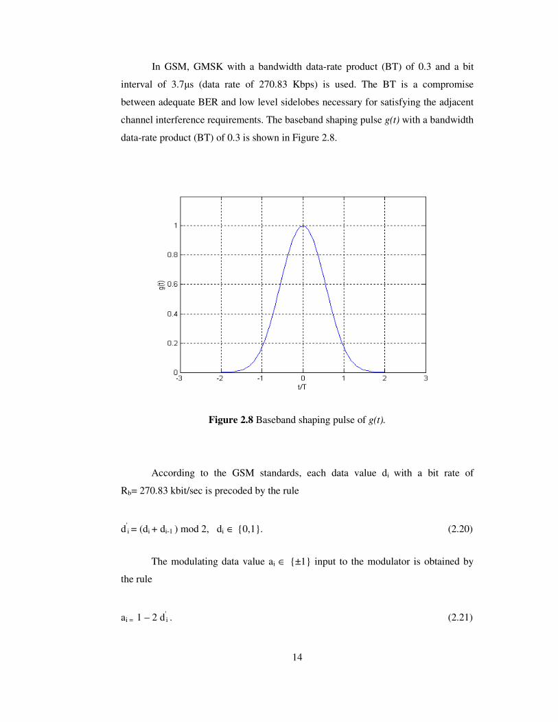
In GSM, GMSK with a bandwidth data-rate product (BT) of 0.3 and a bit
interval of 3.7µs (data rate of 270.83 Kbps) is used. The BT is a compromise
between adequate BER and low level sidelobes necessary for satisfying the adjacent
channel interference requirements. The baseband shaping pulse g(t) with a bandwidth
data-rate product (BT) of 0.3 is shown in Figure 2.8.
Figure 2.8 Baseband shaping pulse of g(t).
According to the GSM standards, each data value di with a bit rate of
Rb= 270.83 kbit/sec is precoded by the rule
d'i = (di + di-1 ) mod 2, di ∈ {0,1}. (2.20)
The modulating data value ai ∈ {±1} input to the modulator is obtained by
the rule
ai = 1 – 2 d'i . (2.21)

15
Figure 2.9 summarizes the generation of GMSK signal.
di ai φ (t) s (t)
Figure 2.9 Generation of GMSK modulated signal.
Linear Approximation of GMSK
As mentioned before, GMSK modulation type belongs to the class of CPM. This
modulation type is essentially nonlinear and hence classical MLSE algorithms for
receiver side cannot work with the form of GMSK. It has been shown in the
literature that every CPM signal can be represented approximately in linear
quadrature amplitude modulation (QAM) signal format by adapting a suitable pulse
shape [7].
In [7], [8] and [9], it is shown that complex envelope of a GMSK modulated
signal, s(t) is exactly constructed by superposition of Nc = 2 L-1 impulses CK..
1
,0
( ) exp[ ] ( )c
o
N
K n k
n n K
s t j hA C t nTπ−∞
= =
= −∑ ∑ , (2.22)
with
0
1
, ,1
.n L
K n i n l K l
i n l
A d d α−
−= =
= −∑ ∑ , (2.23)
where ,K lα ‘s are solved from
Differential encoding
Transmitter filter
Phase modulation

16
11
,1
2L
l
K l
l
K α−
−
=
=∑ , ,K lα ∈{0,1}, K=0, 1,…. Nc-1. (2.24)
The data sequence is defined for n ≥ no, This representation can be used for all
CPM signals For example the complex envelope of a MSK signal (L=1) can be
written as follows:
( )0 0
0expn
MSK i MSK
n n i n
s j h a C t nTπ∞
= =
= −
∑ ∑ , (2.25)
where 0MSKC is a one half cycle sinusoidal with duration of two symbol period. (2.25)
is the well known representation of MSK as OQPSK modulation.
For GMSK with L=3 the exact superposition is made by four impulses [10].
( )0 0
4
0 ,0 1
exp exp ( )n
GMSK i K n K
n i n n n K
s j h a C t nT j hA C t nTπ π∞ ∞
= = = =
= − + −
∑ ∑ ∑∑ , (2.26)
= slin (t) + snl (t). (2.27)
In [9], it is concluded that the GMSK modulated signal sGMSK is the sum of a
term slin (t) and of a term snl (t). Term slin (t) can be interpreted as a linear mapping of
the bit sequence ai to waveforms. On the other hand, term snl (t) causes the
nonlinearity of the GMSK modulation with regard to the general definition of a
linear modulation method. In Figure 2.10, the first two impulses C0 and C1 for
GMSK are displayed. (See also Appendix B)

17
Figure 2.10 Comparison of C0 (t) and C1 (t).
Since C0 has 99% of the signal energy [9], the following linear approximation
is possible:
sGMSK ≈ slin (t)= ( )
0
0GMSK n
n n
s z C t nT∞
=
= −∑ , (2.28)
where
{ }0
exp -1, 1, -j, jn
n i
i n
z j h aπ=
= ∈
∑ , (2.29)
are the symbols determined by the accumulated data stream ai. Only Co(t) is used for
pulse shaping. This approximation of the GMSK modulation is very similar to a PSK
18
or QAM signal. This approximated GMSK has the advantage that it can be realized
with a ordinary I/Q-Modulator as used for PSK or QAM [9] , [10].
The GMSK modulated signal in baseband can be expressed as;
( )0 0
0( ) exp2
n
b i
n n i n
s t j a C t nTπ∞
= =
= −
∑ ∑ , (2.30)
where C0(t) denotes the real-valued pulse shaping function and ai‘s ∈ {±1} are the
input data bits to the modulator.
Effects of the Linear Approximation to GMSK:
The approximation of the GMSK causes a change of the scatter diagram and the
power density spectrum.
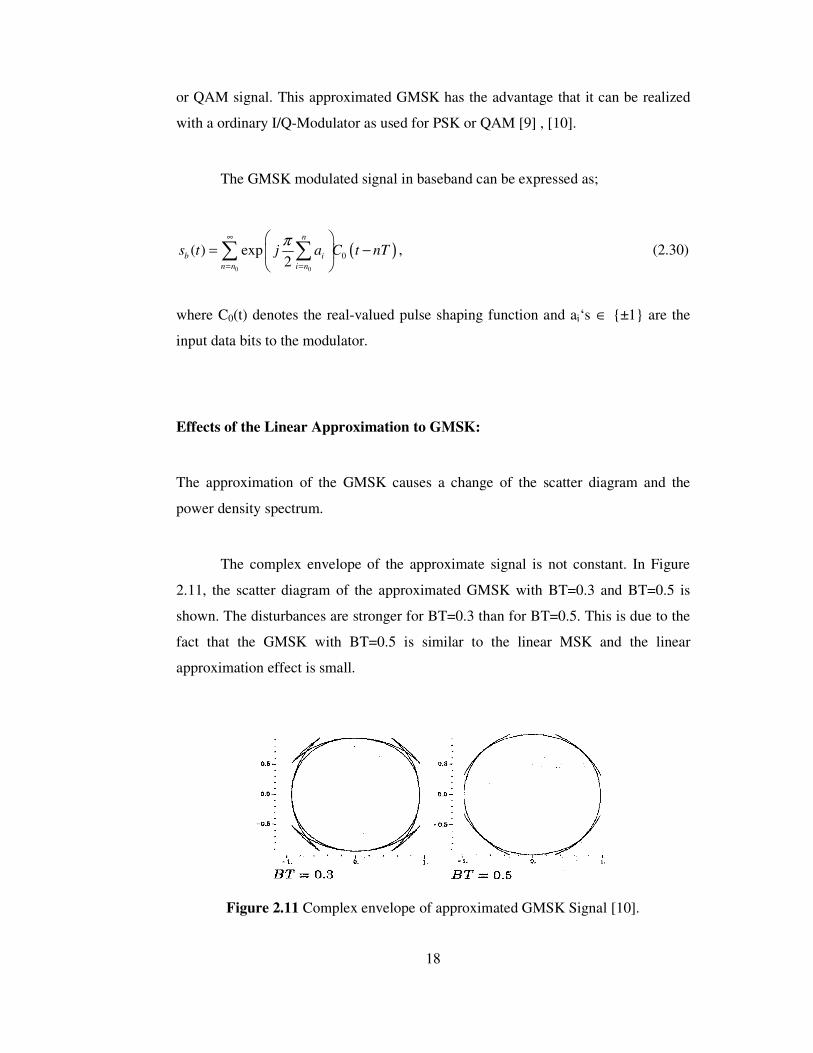
The complex envelope of the approximate signal is not constant. In Figure
2.11, the scatter diagram of the approximated GMSK with BT=0.3 and BT=0.5 is
shown. The disturbances are stronger for BT=0.3 than for BT=0.5. This is due to the
fact that the GMSK with BT=0.5 is similar to the linear MSK and the linear
approximation effect is small.
Figure 2.11 Complex envelope of approximated GMSK Signal [10].
19
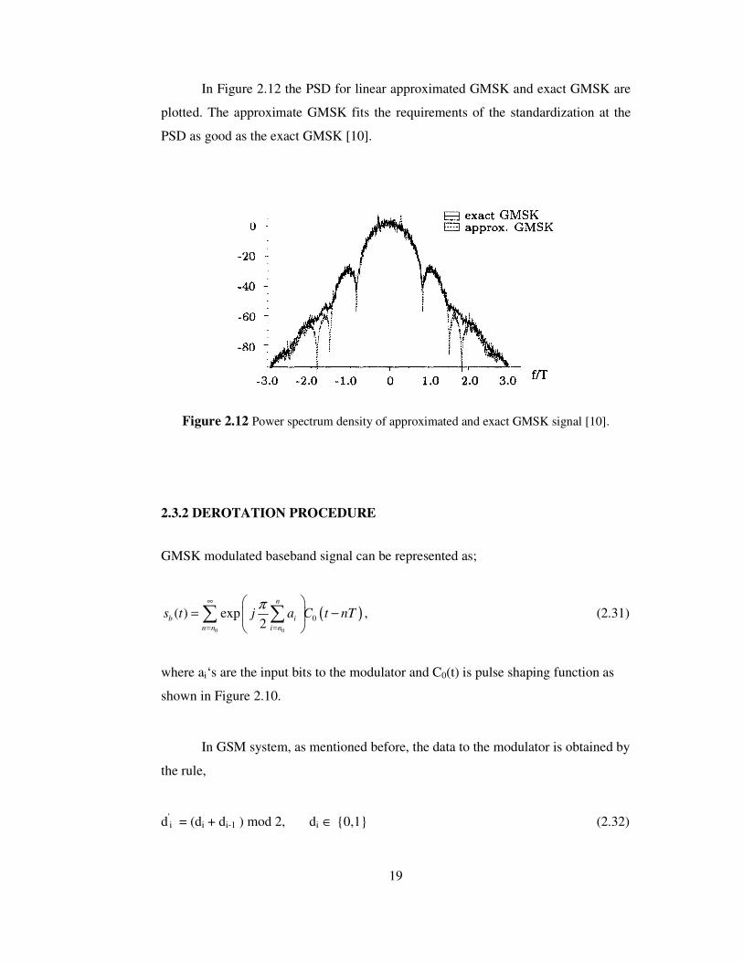
In Figure 2.12 the PSD for linear approximated GMSK and exact GMSK are
plotted. The approximate GMSK fits the requirements of the standardization at the
PSD as good as the exact GMSK [10].
Figure 2.12 Power spectrum density of approximated and exact GMSK signal [10].
2.3.2 DEROTATION PROCEDURE
GMSK modulated baseband signal can be represented as;
( )0 0
0( ) exp2
n
b i
n n i n
s t j a C t nTπ∞
= =
= −
∑ ∑ , (2.31)
where ai‘s are the input bits to the modulator and C0(t) is pulse shaping function as
shown in Figure 2.10.
In GSM system, as mentioned before, the data to the modulator is obtained by
the rule,
d'i = (di + di-1 ) mod 2, di ∈ {0,1} (2.32)

20
where d'i’s are original data bits.
ai = 1 – 2 d'i , ai ∈ {±1} (2.33)
where ai’ s are inputs to the modulator.
The following procedure gives the same result as the above procedure;
ci = 1 – 2 di , (2.34)
ai = ci ci-1 , (2.35)
where ci‘s ∈ {±1} are the original bits which are intended to be decoded in the
receiver side.
GMSK modulated baseband signal is then given by
( )0 0
1 0( ) exp2
n
b i i
n n i n
s t j c c C t nTπ∞
−= =
= −
∑ ∑ , (2.36)
( )0 0
1 0( ) exp2
n
b i i
n n i n
s t j c c C t nTπ∞
−= =
= −
∑∏ . (2.37)
Because the term ‘cici-1’ is either -1 or +1, exp ( j π/2 cici-1) is either exp (j
π/2)= j or exp ( - j π/2)= - j, thus exp ( j π/2 cici-1) = j cici-1:
( )0 0
1 0( )n
b i i
n n i n
s t jc c C t nT∞
−= =
= −∑∏ (2.38)
( )0
0 0
11 0( )
nn n
b i i
n n i n
s t j c c C t nT∞
− +
−= =
= −∑ ∏ (2.39)

21
0
0 0
12
1 1
n n
i i n n i
i n i n
c c c c c−
− −= =
=∏ ∏ . (2.40)
Because ci 2 =1 for all i,
0
0
1 1
n
i i n n
i n
c c c c− −=
=∏ , (2.41)
( )0
0
0
11 0( ) n n
b n n
n n
s t j c c C t nT∞
− +
−=
= −∑ . (2.42)
( )0
0
0
11 0( ) n n
b n n
n n
s t j c j c C t nT∞
− +
−=
= −∑ (2.43)
Assuming the terms 0 1nc − =1 and 0( 1)n
j− + =1 which are independent of n, it is
convenient to express the GMSK modulated signal as follows;
( )0
0( ) n
b n
n n
s t j c C t nT∞
=
= −∑ . (2.44)
(2.44) can be expressed in discrete-time domain as follows;
0
0i i n
n
b n
n n
s j c C−
∞
=
= ∑ . (2.45)
The signal at the receiver will have passed through a frequency selective
channel and a receiver filter in order to reject the out of band components. Let gR[n]
denotes the discrete -time equivalent of receiver filter impulse response and hc[n]
denotes the discrete-time equivalent of the channel impulse response. The received
signal in baseband (absence of noise) can be expressed as follows;
22
=ir0
n
n i n
n n
j c h∞
−=
∑ , (2.46)
where h[n]= C0 [n] * hc[n]* gR[n] is the overall impulse response of the system from
the output of the encoder to the detector input.
Equation (2.44) shows that the received signal samples can be obtained by
convolving the input data with the overall system impulse response h[n] and then
applying a π /2 phase rotation on a complex plane from symbol to symbol basis.
Phase rotation can be avoided by multiplying the received signal by the
complex function q [i]=(-j)i . The sequence q [n] is called derotation sequence.
Multiplying r [i] by the derotation sequence r´ [i] is obtained:
jn = (-j) –n =(-j) i-n (-j)-i, (2.47)
ni
ni
n
n
i
i hjcjr −−− −−= ∑ )()( , (2.48)
r´ [i] = r [i] q[i ], (2.49)
ni
ni
n
ni hjcr −−−=∑ )(' . (2.50)
The derotated channel impulse response is h' [i] = h[i].q[i] = h i (-j) i :
h' i-n = h i-n (-j) i-n. (2.51)
Therefore,
ni
n
niii hcqrr −∑== '' . (2.52)
23
By applying this derotation operation, the rotational structure of the signal is
removed and a standard linear QAM structure model can be obtained.
2.3.3. MLSE Receiver, Viterbi Algorithm and Channel Identification
The classical MLSE receiver generally consists of an ML sequence estimator
implemented by the Viterbi Algorithm. Viterbi algorithm uses the knowledge of
channel characteristics and the received signal in order to find the most likely
transmitted data sequence.
The form of r´ [i] given in equation (2.50) allows classical MLSE detection of
the transmitted data sequence c by the use of Viterbi Algorithm. In the sequel, the
subscripts indicating the derotation will be dropped for simplicity. The Viterbi
Algorithm needs the knowledge of the channel impulse response (CIR).
A training sequence is used to produce an estimate of CIR at the receiver.
This estimate is used in the demodulation process to equalize the effects of multipath
propagation.
In GSM standards, the training sequence is placed at the centre of each burst
to minimize the error in the information bits farthest from the training sequence.
Consequently, the first section of the burst must be stored.
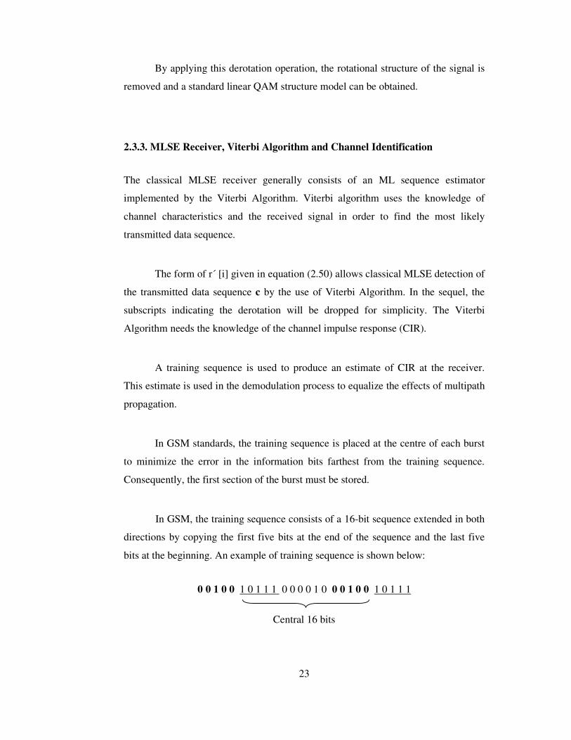
In GSM, the training sequence consists of a 16-bit sequence extended in both
directions by copying the first five bits at the end of the sequence and the last five
bits at the beginning. An example of training sequence is shown below:
0 0 1 0 0 1 0 1 1 1 0 0 0 0 1 0 0 0 1 0 0 1 0 1 1 1
Central 16 bits

24
The central 16 bits are chosen to have a highly peaked autocorrelation
function, following GMSK modulation, and the repeated bits at either end ensure that
the resulting channel estimate may be up to five bits wide before being corrupted by
the information bits.
GSM specifications define eight different training sequences for using in a
normal burst, each with low cross-correlation properties following GMSK
modulation. Consider the case of two similar simultaneous signals arriving at the
receiver at the same time one of them is interference. If their training sequences are
identical, there is no way to distinguish the contribution of each to the received
signal. When training sequences are different and are as little correlated as possible,
the situation is much clearer.
Each training sequence is described by a training sequence code (TSC). A list
of the TSC is given in Table 2.1.
Table 2.1 Training sequence codes.
Training sequence code (TSC) Training sequence bits
0 0,0,1,0,0,1,0,1,1,1,0,0,0,0,1,0,0,01,0,0, 1,0,1,1,1
1 0,0,1,0,1,1,0,1,1,1,0,1,1,1,1,0,0,0,1,0,1,1,0,1,1,1
2 0,1,0,0,0,0,1,1,1,0,1,1,1,0,1,0,0,1,0,0,0,0,1,1,1,0
3 0,1,0,0,0,1,1,1,1,0,1,1,0,1,0,0,0,1,0,0,0,1,1,1,1,0
4 0,0,0,1,1,0,1,0,1,1,1,0,0,1,0,0,0,0,0,1,1,0,1,0,1,1
5 0,1,0,0,1,1,1,0,1,0,1,1,0,0,0,0,0,1,0,0,1,1,1,0,1,0
6 1,0,1,0,0,1,1,1,1,1,0,1,1,0,0,0,1,0,1,0,0,1,1,1,1,1
7 1,1,1,0,1,1,1,1,0,0,0,1,0,0,1,0,1,1,1,0,1,1,1,1,0,0
Figure 2.13 shows the autocorrelation function of one of these eight training
sequences calculated between the central 16 bits and the whole 26-bit sequence. The
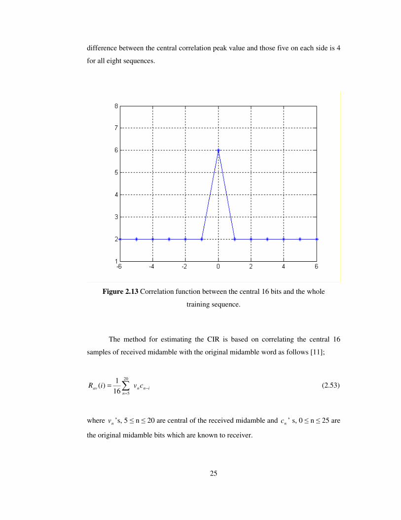
25
difference between the central correlation peak value and those five on each side is 4
for all eight sequences.
Figure 2.13 Correlation function between the central 16 bits and the whole
training sequence.
The method for estimating the CIR is based on correlating the central 16
samples of received midamble with the original midamble word as follows [11];
inn
n
av cviR −=
∑=20
516
1)( (2.53)
where nv ’s, 5 ≤ n ≤ 20 are central of the received midamble and
nc ’ s, 0 ≤ n ≤ 25 are
the original midamble bits which are known to receiver.
26
The performance of the MLSE receiver is dependent on the available estimate
of the channel impulse response. If the training sequence is placed in front of the
burst channel impulse response will be obtained by the same correlation method, but
performance of estimating CIR is not as good as the case of the training sequence is
placed in the centre of each burst. [12].
The received signal without noise can be expressed as
∑ −=n
nini hcr . (2.54)
With the assumption that the function h(t) is known, the received signal for
each possible sequence may be reconstructed. The reconstructed complex signal for
the mth sequence is denoted as
[ ] [ ] [ ]nicncjisn
mnm
b −=∑∞
=0
0
. (2.55)
The MLSE algorithm attempts to find the transmitted sequence (cm) that
maximizes the log likelihood function [3].
The one among all the possible vectors c which maximizes LLF is the direct
solution of the maximization problem. But this is not an efficient solution method
especially when c gets larger. In order to reduce computational load Viterbi
algorithm can be used.
The proposed symbol synchronizer presented in section 4.3 depends on the
performance of Viterbi algorithm. Throughout the study, the perfect estimation of the
channel estimation is assumed and tentative decisions from Viterbi algorithm are
assumed to be error free.
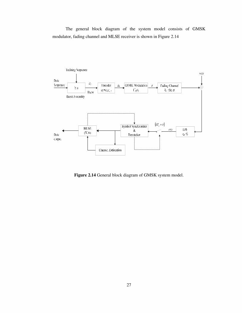
27
The general block diagram of the system model consists of GMSK
modulator, fading channel and MLSE receiver is shown in Figure 2.14
{ }τ+skT
Figure 2.14 General block diagram of GMSK system model.
28
CHAPTER 3
SYMBOL SYNCHRONIZATION REVIEW
3.1 INTRODUCTION
Timing recovery is one of the most critical functions that are performed at the
receiver of a synchronous digital communication system. The receiver must know
not only the frequency at which the outputs of the demodulators are sampled, but
also where to take the samples within each symbol interval.
In this chapter, firstly the definition of symbol synchronization is presented.
Secondly, a review of symbol timing recovery (STR) methods is given to highlight
the attributes. In the context of this review, a brief history of timing recovery with
some applications on MSK signals is included. Finally, the maximum likelihood
estimation of the timing recovery is presented.
3.2 SYMBOL TIMING RECOVERY
In a digital communication system, the output of the baseband filter (a matched
filter) must be sampled periodically at the precise sampling time instants that
minimize the detector error probability. The process of extracting the clock signal for
determining the accurate locations of the maximum eye openings for reliable
29
detection is usually called symbol synchronization or symbol timing recovery (STR).
A system that is able to estimate such locations is called a timing (or) clock
synchronizer.
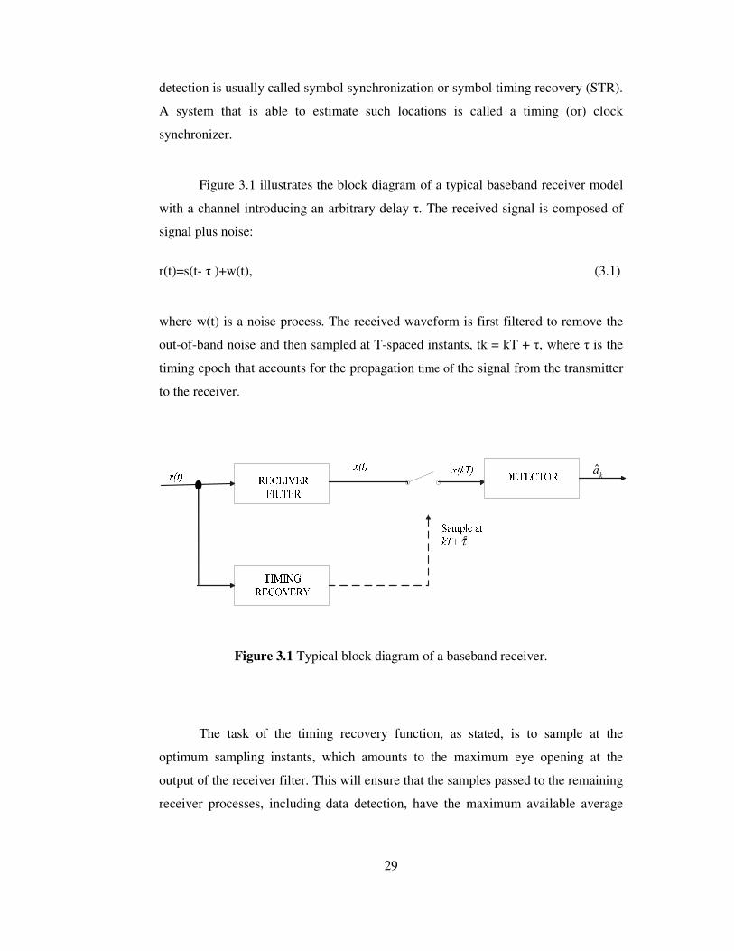
Figure 3.1 illustrates the block diagram of a typical baseband receiver model
with a channel introducing an arbitrary delay τ. The received signal is composed of
signal plus noise:
r(t)=s(t- τ )+w(t), (3.1)
where w(t) is a noise process. The received waveform is first filtered to remove the
out-of-band noise and then sampled at T-spaced instants, tk = kT + τ, where τ is the
timing epoch that accounts for the propagation time of the signal from the transmitter
to the receiver.
τ
ka
Figure 3.1 Typical block diagram of a baseband receiver.
The task of the timing recovery function, as stated, is to sample at the
optimum sampling instants, which amounts to the maximum eye opening at the
output of the receiver filter. This will ensure that the samples passed to the remaining
receiver processes, including data detection, have the maximum available average
30
signal-to-noise ratio (SNR) and hence a bit error rate (BER) as close as possible to
optimum.
3.2.1 Existing STR Schemes
The books written by Meyr and Ascheid [13], Meyr, Moeneclaey and Fechtel [14],
and Mengali and D’Andrea [15] are excellent references in the symbol
synchronization literature.
Existing symbol synchronizers are modeled with analog or digital methods.
Due to a time shift between transmitter and receiver, samples at t=kT+ τ are required.
In analog methods continuous- time waveforms are operated on. In digital method, in
order to perform the recovery of the timing epoch signal samples taken at a suitable
rate are processed. Main emphasis is given to digital timing recovery in this section.
From the operating principle point of view, two categories of synchronizers
are distinguished, i.e. error tracking (or feed back, or closed loop ) synchronizers and
feedforward (or open loop) synchronizers. Feedback configuration and Feedforward
configuration are shown in Figure 3.2 and 3.3.
In both configurations anti alias filter (AAF) limits the bandwidth of the
received waveform. Sampling is controlled by a fixed clock whose ticks are not
locked to the incoming data. The bulk of the pulse shaping is performed in the
matched filter whose location is not necessarily that shown in the figures. The MF
may be moved inside the loop in Figure 3.2 or it may be shifted so as to have a
common input with the timing estimator in Figure 3.3 [15].

31
Figure 3.2 Feedback configuration.
Figure 3.3 Feedforward Configuration.
Timing correction is akin to the operation of a voltage controllable delay line
and produces synchronized samples to be used for decision and synchronization
purposes. Timing correction is generally performed with interpolators with the
desired interpolation times {tk}.
In feedback configuration timing corrector feeds a timing error detector
(TED) whose purpose is to generate an error signal e(k) proportional to the
difference between τ and its current estimate. The error signal is then exploited to
recursively update the timing estimates. The error signal is then filtered to reduce the
32
variance of the timing error and the output is used to recursively update the timing
estimates.
On the other hand, feedforward methods derive an estimate of the timing
epoch by applying a non-linear process to the received signal samples. The estimate
is used to adjust the sample timing to the optimum location.
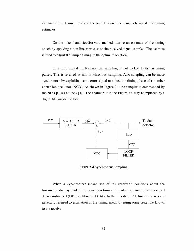
In a fully digital implementation, sampling is not locked to the incoming
pulses. This is referred as non-synchronous sampling. Also sampling can be made
synchronous by exploiting some error signal to adjust the timing phase of a number
controlled oscillator (NCO). As shown in Figure 3.4 the sampler is commanded by
the NCO pulses at times { tn}. The analog MF in the Figure 3.4 may be replaced by a
digital MF inside the loop.
MATCHED FILTER
r(t) y(t) To datadetector
NCO
TED
LOOP FILTER
y(tk)
{tk}
e(k)
Figure 3.4 Synchronous sampling.
When a synchronizer makes use of the receiver’s decisions about the
transmitted data symbols for producing a timing estimate, the synchronizer is called
decision-directed (DD) or data-aided (DA). In the literature, DA timing recovery is
generally referred to estimation of the timing epoch by using some preamble known
to the receiver.
33
When a synchronizer determines the timing phase error without using
knowledge of the transmitted data values, the synchronizer is called non-decision-
directed (NDD) or non-data aided, (NDA).
Next section gives the details of the research on symbol synchronization in
CPM signals.
3.2.2 Symbol Synchronization in CPM Signals
MSK and GMSK are subsets of the continuous phase modulation (CPM) schemes as
explained in Appendix A. This section gives a history of timing recovery with CPM
signals especially with MSK and GMSK signals.
Symbol timing recovery for CPM signals has been first discussed by de Buda
[16], specifically for minimum shift keying (MSK), where a nonlinearity is used to
generate tones at the clock frequency. This algorithm was further analyzed in some
papers and in [17] it has been shown that it can be used for any CPM signal. The
problem with these Buda-like [18] synchronizers is their poor performance with the
smoothed frequency pulses.
A decision-directed (DD) algorithm based on the maximum likelihood (ML)
techniques is proposed in [19] using MSK modulation. The method provides the joint
ML estimation of carrier phase, timing epoch and data, but suffers from spurious
locks in the maximization of the likelihood function.
In order to solve the problems related with the mentioned algorithms some
NDA structures are developed. In [20],[21],[22] feedforward NDA algorithms are
discussed. Two of these methods, proposed by Mehlan, Chen and Meyr [20] and
Lambrette and Meyr [21], recover the clock signal in an ad hoc manner by passing
the received signal samples through a nonlinearity and a digital filter. The algorithm

34
behind this ad-hoc scheme obtained specifically for pure MSK and not applicable to
any other CPM format. In a different approach, [22], the non-data-aided recovery is
obtained by applying maximum likelihood methods. Although it is simple and seems
suitable for burst mode transmission the algorithm is obtained under the assumption
of low SNR. This results in the deviation from the desired performance even in the
moderate SNR values.
Although, it is widely believed that conventional clock synchronizers can be
used even with fading channels, a closer look at the question may be worthwhile. In
[20] and [23], the effects of a flat fading channel are taken in consideration with the
symbol synchronizer employing nonlinearity and filtering in a feedforward manner.
Also, the effect of frequency- selective channels is tested in [20], and a dramatic
degradation is found in the bit error rate.
3.3 MAXIMUM LIKELIHOOD TIMING ESTIMATION
It is widely recognized that maximum likelihood (ML) estimation techniques offer a
systematic and conceptually simple guide to the solution of synchronization
problems and they provide optimum or nearly optimum solutions.
In this section the framework for maximum likelihood symbol timing
recovery is established since most of the algorithms have been discovered by
application of the ML estimation [24]. This is also the case for the proposed
algorithm given in Section 4.3. The general formulation of the ML timing estimation
is discussed in detail in [15] and [25].
Considering the baseband equivalent of the bandpass signal, the received
signal in (3.1) can be described as
)(),()( twtstr l += τ , (3.2)
35
where τ represents an arbitrary delay introduced by the channel to the transmitted
signal ls (t) . The notation ls (t,τ) is adopted to stress the dependence of the signal on
the timing epoch. w(t) is white Gaussian noise with spectral height 0N /2 .
The ultimate goal of a symbol synchronizer is to estimate the most likely
value of the timing epoch. This is accomplished when synchronizer maximizes the
aposteriori probability for all values of τ:
{ }|rˆ arg max ( | )MAP p r(t)τ
τ
τ τ= , (3.3)
given the observed signal r(t) [26].
ML estimation requires the determination of the signal r(t) which maximizes
the conditional probability density function lr\s lp (r(t)\s (t,τ)) , that is, the most likely
signal, ls (t,τ) , which produces the received signal, r(t) , over a specific observation
period To.
We can rewrite the a posteriori probability using Bayes’ theorem:
|r r|
r
( )( | ) (r(t)| )
( ( ))
pp r(t) p
p r t
ττ τ
ττ τ= , (3.4)
where rp (r(t)) describes the probability that r(t) was received, and τp (τ) describes
the probability that ls (t,τ) was transmitted with a delay of τ. In this case τp (τ) is a
constant assuming the time delay has a uniform pdf over the interval [0,T]. In
addition, rp (r(t)) is simply a normalized constant.
36
Let r , ls (τ) and w be the vector representations of r(t) , ls (t,τ) and w(t)
over a complete orthonormal set { }K
i i=1(t)φ . Then, the i-th component of r is given by
[26] as
0
( ) ( )i i
T
r r t t dtφ= ∫ , (3.5)
where 0T devotes the observation interval. Similarly,
0
( ) ( , ) ( )li l i
T
s s t t dtτ τ φ= ∫ , (3.6)
0
( ) ( )i i
T
w w t t dtφ= ∫ , (3.7)
The standard form of the pdf for the sum of a known signal and AWGN, is
2
r|
00
( ( ))1( | ) exp i li
i
r sp r
NNτ
ττ
π
− −=
, (3.8)
As the additive noise is considered to be white, the observations of noise,
iw ’s, are independent, that is,
{ } )(2
0 jiN
wwE ji −= δ , (3.9)
Hence, the pdf may be expanded over K components by taking the product of
the pdfs for the individual sample observations and leads to the desired result
37
( )
2
r|1 0
0
( ( ))1( | ) exp
Ki li
Ki
r sp r
NNτ
ττ
π =
− −=
∏ , (3.10)
within the observation interval T0. To simplify the likelihood function the natural
logarithm may be taken, which after some rearrangement, results in
2r|
10
1ln ( | ) ( ( ))
K
i li K
i
p r r s CN
τ τ τ=
= − − + ∑ , (3.11)
where
( )
=
KK
NC
0
1ln
π, (3.12)
Equation (3.11) can be converted to the continuous time domain form by
dropping the constant CK as it is independent of the time delay and taking the limit as
K→∞. Then, the result is
0
2
0
1( | ) ( ( ) ( , ))L l
T
r r t s t dtN
τ τΛ = − −∫ , (3.13)
where ( | )L r τΛ is the continuous time log likelihood function (LLF). The squared
term within the integral is a measure of the distance between the received and
reference signals. Only the cross-correlation term in (3.13) contains useful
information regarding the time epoch. )(2 tr is independent of τ, and the ),(2 τtsl term
is simply the power of the transmitted signal during the observation interval T0.
Consequently, the most likely timing offset τ can be expressed as the value of
τ which maximizes

38
00
2( | ) ( ) ( , )L l
T
r r t s t dt constN
τ τΛ = +∫ , (3.14)
that is,
{ }00
2ˆ arg max ( | ) arg max ( ) ( , )L l
T
r r t s t dtNτ τ
τ τ τ
= Λ =
∫ . (3.15)
The constant term is not included in (3.15), as it does not affect the
maximization process. The synchronization scheme investigated in this thesis is
based on the final expression and the details are provided in the next chapter.
39
CHAPTER 4
A DD STR BASED ON MATCHED FILTERING FOR GMSK
SIGNALS
4.1 INTRODUCTION
Synchronizer is one of the most critical receiver functions and comparison of the
performance of the synchronizers with a reference bound is an important point.
Therefore, this chapter starts with the presentation of Modified Cramer Rao Bound
(MCRB) and Mazo Criterion. Modified Cramer Rao Bound (MCRB) is commonly
used under AWGN channel as a bound. In [1], minimum squared ISI (msISI)
criterion and Mazo criterion are presented as an optimum value criteria for
considering fading channel effects. As a result similarity between msISI criterion and
Mazo criterion is emphasized. In this study, the criterion proposed by Mazo [28] is
used as optimum timing phase criteria under Rayleigh fading channel.
Transmission over frequency selective fading channel necessitates
specifically designed synchronizer structures and algorithms that are different from
those for static channel. In the second part of this chapter, the proposed timing
recovery scheme based on the method of ML estimation of the timing epoch in [1] is
reviewed. The proposed timing recovery scheme does not employ any feedback loop
so that it does not suffer from hang-up problems which are common in feedback
schemes. Correlation (matched filter) method is used for the recovery of the timing
epoch. In order to determine fractional delays correlation between the received signal
and the reference samples is interpolated and an iterative maximum search is
40
performed. Finally a discussion on the performance of the proposed timing recovery
scheme for GMSK is given.
4.2. CRITERIA FOR TIMING PHASE
4.2.1. Modified Cramer Rao Bound
In the literature considerable number of technical papers makes use of the modified
Cramer–Rao bounds (MCRB’s) for timing estimation as benchmarks. Cramer-Rao
bound is a lower limit to the variance of any unbiased estimator.
{ } )()(ˆ τττ CRBrVar ≥− , (4.1)
Let τ(r) be estimation of τ . τ(r) depends on the observation r .
Cramer-Rao bound is expressed as
2
2
1( )
ln ( | )r
CRBr
E
ττ
τ
∆
=− ∂ Λ
∂
, (4.2)
=2
1
ln ( | )r
rE
τ
τ
∂ Λ ∂
.
Unfortunately, application of the bound to synchronization problems leads to
serious mathematical difficulties. MCRB’s are much easier to employ, but are loose
than true CRB’s. The relation between the bounds is
{ } )()()(ˆ ττττ MCRBCRBrVar ≥≥− . (4.3)
41
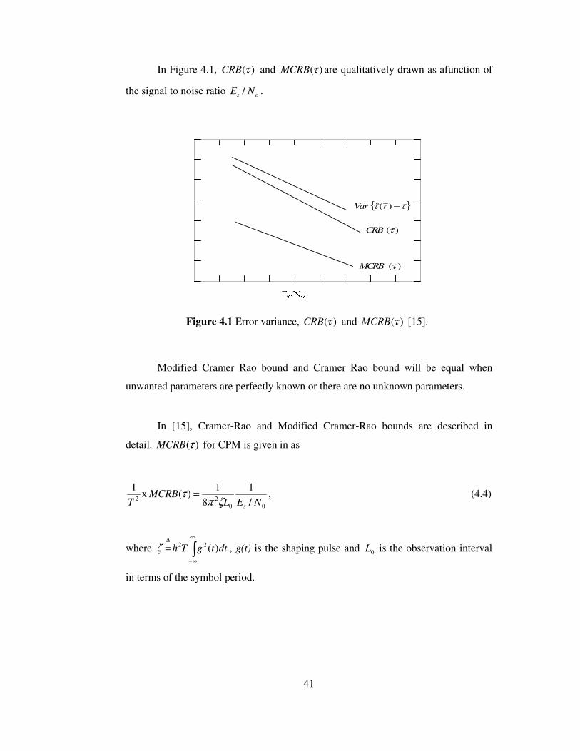
In Figure 4.1, ( )CRB τ and ( )MCRB τ are qualitatively drawn as afunction of
the signal to noise ratio /s oE N .
{ }ττ −)(ˆ rVar
)(τCRB
)(τMCRB
Figure 4.1 Error variance, ( )CRB τ and ( )MCRB τ [15].
Modified Cramer Rao bound and Cramer Rao bound will be equal when
unwanted parameters are perfectly known or there are no unknown parameters.
In [15], Cramer-Rao and Modified Cramer-Rao bounds are described in
detail. )(τMCRB for CPM is given in as
2
1
Tx
002 /
1
8
1)(
NELMCRB
sζπτ = , (4.4)
where ∫∞
∞−
∆
= dttgTh )(22ζ , g(t) is the shaping pulse and 0L is the observation interval
in terms of the symbol period.
42
For MSK:
≤≤
=
,,0
,0,2
1)(
elsewhere
TtTtg (4.5)
Thus (4.4) reduces to a simple form
2
1
Tx
002 /
12)(
NELMCRB
sπτ = , (4.6)
To find )(τMCRB for GMSK, equation (4.4) is used with pulse shaping
1 2 ( / 2) 2 ( / 2)( )
2 ln 2 ln 2
B t T B t Tg t erf erf
T
π π − += − + −
. (4.7)
4.2.2 Mazo Criterion
In this criterion, optimum timing phase is defined as the one which results in the least
MMSE, at the output of an equalizer. For most transmission systems the bandwidth
is greater than 1/2T where T is the symbol period. Therefore, when it is sampled at a
rate 1/T, the sampling phase will change the equivalent system response by canceling
or augmenting the aliased components. It has been shown by Mazo [28] that for a
system consisting of a channel, a sampler and a forward linear equalizer the optimum
timing is found by maximizing the equivalent channel magnitude response at the
frequency 1/2T, i.e., at the Nyquist band edge.
The received signal samples at time instants t = kT +τ , can be re-expressed
in the absence of noise by
nk
n
nk ahr −∑= )()( ττ , (4.8)
43
where the notation )()( ττ += nThhn is used. These samples are related to their
discrete Fourier transform as,
dfefHh fnTj
eqn
πττ 2),()( ∫∞
∞−
= , (4.9)
where
τπτ )/(2)/(),( Tnfj
n
eq eTnfHfH +−∑ += , (4.10)
is the equivalent channel response taking folding effects into account due to sampling.
The exponential term in (4.10) reflects the effect of the timing phase. If the
excess bandwidth of the sampled received signal is assumed to be less than 100%,
then
TjTj
eq eTHeTHTH // )2/1()2/1(),2/1( πτπττ −+= − , (4.11)
According to the criterion proposed by Mazo [28], the optimum timing phase
is defined as optτ that maximizes the cost function 2
),2/1( τTH eq and is
approximately given by
[ ] kTTHTHT
opt +−−= ))2/1(arg())2/1(arg(2π
τ , (4.12)
where k is any integer.
The equation derived by Mazo is nothing but the slope of the phase response
between the frequencies {-1/2T, 1/2T}. Correspondingly, the timing phase behaviour

44
given with this relation can be characterized by the slope of the phase response in a
way given in the following formula:
[ ] kTfHfHff
+−−
= ))(arg())(arg()(2
121
21πτ , (4.13)
with Tff 2/121 =−= .
This result directly gives the delay for linear phase systems, and in a sense
may show the general tendency of the time-variant channel.
Figure 4.2 and 4.3 show some examples for the timing values obtained by
equation (4.13) for different 1f and 2f . In Figure 4.2, the variations of the timing
phase are obtained for a multipath channel which corresponds to a variation with a
mobile speed of 50 km/h and a carrier frequency of 900 MHz. In Figure 4.3 a faster
channel exists. The variations of the timing phase are drawn for a multipath channel
which corresponds to a variation with a mobile speed of 90 km/h and a carrier
frequency of 1800MHz.
In Figure 4.2 and Figure 4.3 the curves coincide at some specific interval and
give the same delay. At other instants, the values of timing phase differ for different
frequency pairs. Of course, this depends on the channel characteristics, but gives
some information about the channel variations and the effects on optimum timing
phase.

45
0 500 1000 1500 2000 2500-0.2
-0.1
0
0.1
0.2
0.3
0.4
0.5
t/T
Norm
aliz
ed T
imin
g P
hase
f1= - f
2 =1/4T
f1=-f
2 =1/8T
Figure 4.2 Normalized timing phase obtained from Mazo criterion (v=50 km/h, fc=900 MHz, fd = 42Hz).
0 500 1000 1500 2000 2500-0.2
-0.1
0
0.1
0.2
0.3
0.4
0.5
0.6
0.7
t/T
Norm
aliz
ed T
imin
g P
hase
f1= - f
2 =1/4T
f1= - f
2 =1/8T
Figure 4.3 Normalized timing phase obtained from Mazo criterion
(v=90 km/h, fc=1800 MHz, fd= 150Hz).
46
4.3. PROPOSED DD STR FOR GMSK SIGNALS
A decision-directed timing recovery scheme was proposed in [1] and [2]. It simply
employs a correlation (matched filter) method based on the maximum likelihood
(ML) estimation of the timing epoch. For determining the fractional delays,
interpolation and an iterative maximum search algorithm are used.
4.3.1. Correlation (Matched Filter) Method
In the literature, a large number of algorithms that use several versions of ML
estimators exist. The notion behind the proposed symbol timing estimation algorithm
depends on the theory of maximum likelihood (ML) estimation. The proposed
symbol timing estimator does not give the estimates of the timing offset explicitly. It
is based on the determination of the maximum value of the log likelihood function as
a function of τ , i.e.,
{ })(maxargˆ τττ
LΛ= , (4.14)
Let us rewrite the likelihood function (3.14) obtained in Section 3.3:
∫ −=Λ
0
)()(2
)(0 T
lL dttstrN
ττ , (4.15)
The integral in (4.15) is just a convolution operation. The likelihood function
is simply the output of a filter with impulse response )( tsl − and input )(tr over the
observation interval T0. Then, the estimate of the symbol timing offset may be
obtained by finding the timing instant which corresponds to the maximum of the
output of the cross-correlation between the received and the reference signal
samples. The correlation function can be expressed as
47
∫ −=
0
)()()(T
dutusurtR , (4.16)
and the proper sampling instant is given by
)(maxarg tRtt
samp = , (4.17)
The correlation function can also be viewed as the output of a filter matched
to reference signal when the input is the received signal.
The proposed synchronizer has two main modes: First one is the acquisition
mode and the other one is the tracking mode. In the acquisition mode of the
synchronizer a training sequence is employed. Training sequences can be selected
from Table 2.1. The initial adjustment of the clock is accomplished by finding the
timing instant which corresponds to the maximum of the output of the cross-
correlation between the received and the transmitted signal samples which is formed
by the training sequence.
After the initial adjustment of the clock, in the tracking mode, the channel
variations are tracked in a decision-directed manner using the decisions coming from
the MLSE receiver (Viterbi algorithm). These decisions are referred to as tentative
decisions. The tentative decisions are used to form a filter matched to the GMSK
waveform. The correlation function defined in (4.16) is obtained from the output of
the matched filter with its input being the received signal. The timing epoch is
estimated by determination of the instant corresponding to the maximum of the
matched filter output. Estimated timing epoch is in terms of sampling time, in order
to obtain fractional timing epoch interpolation and an iterative maximum search
algorithm are used.
As a summary the general flow of the proposed timing recovery process is
shown in Figure 4.4. The received samples are first taken into the data buffer and
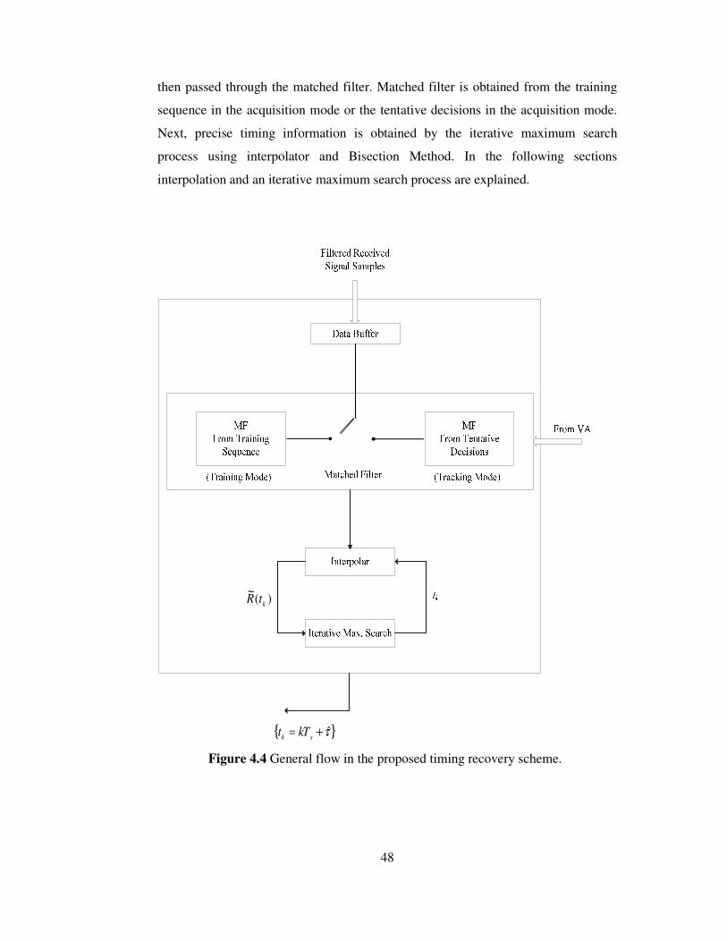
48
then passed through the matched filter. Matched filter is obtained from the training
sequence in the acquisition mode or the tentative decisions in the acquisition mode.
Next, precise timing information is obtained by the iterative maximum search
process using interpolator and Bisection Method. In the following sections
interpolation and an iterative maximum search process are explained.
)(~
ktR
{ }τ+=sk
kTt
Figure 4.4 General flow in the proposed timing recovery scheme.
49
4.3.2. Iterative Maximum Search
In determining the maximum of the correlation function, a simple and satisfactory
iterative process based on Bisection Method is employed. The iteration method
presented here is the same to the one used in [1].
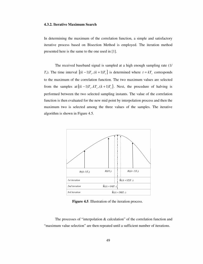
The received baseband signal is sampled at a high enough sampling rate (1/
Ts). The time interval [ ]ss TkTk )1(,)1( +− is determined where skTt = corresponds
to the maximum of the correlation function. The two maximum values are selected
from the samples at{ }sss TkkTTk )1(,,)1( +− . Next, the procedure of halving is
performed between the two selected sampling instants. The value of the correlation
function is then evaluated for the new mid point by interpolation process and then the
maximum two is selected among the three values of the samples. The iterative
algorithm is shown in Figure 4.5.
1st iteration
2nd iteration
3rd iteration
R((k-1)Ts) R(kTs) R((k+1)Ts)
)1/2)T((R~
s+k
)1/4)T((R~
s+k
)3/8)T((R~
s+k
Figure 4.5. Illustration of the iteration process.
The processes of “interpolation & calculation” of the correlation function and
“maximum value selection” are then repeated until a sufficient number of iterations.
50
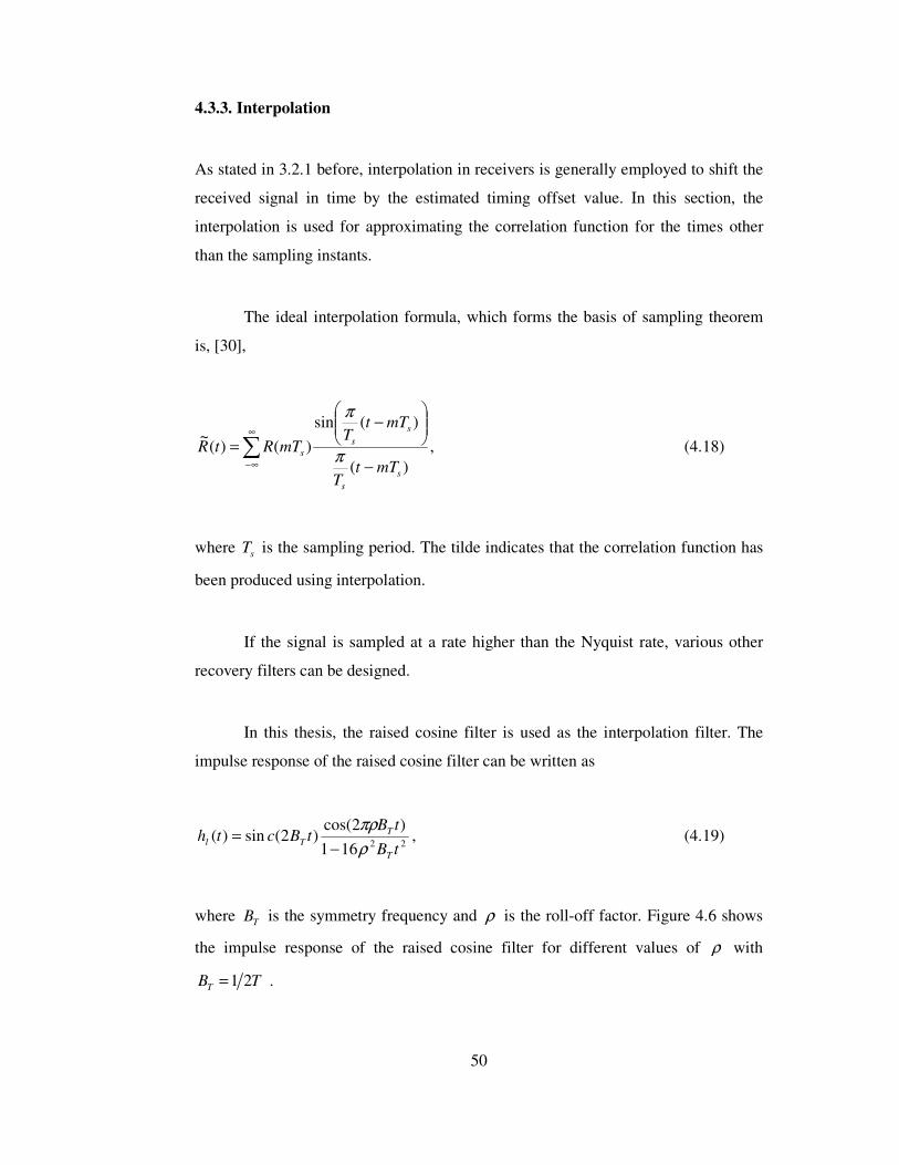
4.3.3. Interpolation
As stated in 3.2.1 before, interpolation in receivers is generally employed to shift the
received signal in time by the estimated timing offset value. In this section, the
interpolation is used for approximating the correlation function for the times other
than the sampling instants.
The ideal interpolation formula, which forms the basis of sampling theorem
is, [30],
)(
)(sin
)()(~
s
s
s
s
s
mTtT
mTtT
mTRtR
−
−
=∑∞
∞−π
π
, (4.18)
where sT is the sampling period. The tilde indicates that the correlation function has
been produced using interpolation.
If the signal is sampled at a rate higher than the Nyquist rate, various other
recovery filters can be designed.
In this thesis, the raised cosine filter is used as the interpolation filter. The
impulse response of the raised cosine filter can be written as
22161
)2cos()2(sin)(
tB
tBtBcth
T
T
Tlρ
πρ
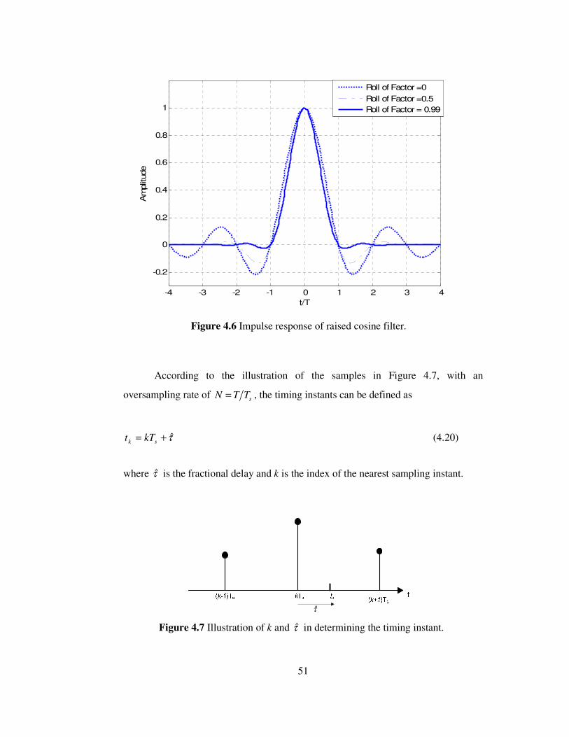
−= , (4.19)
where TB is the symmetry frequency and ρ is the roll-off factor. Figure 4.6 shows
the impulse response of the raised cosine filter for different values of ρ with
1 2TB T= .
51
-4 -3 -2 -1 0 1 2 3 4
-0.2
0
0.2
0.4
0.6
0.8
1
t/T
Am
plit
ude
Roll of Factor =0
Roll of Factor =0.5
Roll of Factor = 0.99
Figure 4.6 Impulse response of raised cosine filter.
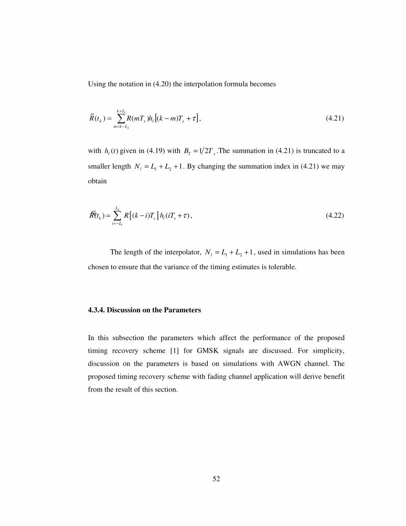
According to the illustration of the samples in Figure 4.7, with an
oversampling rate of sN T T= , the timing instants can be defined as
τ+= sk kTt (4.20)
where τ is the fractional delay and k is the index of the nearest sampling instant.
τ
Figure 4.7 Illustration of k and τ in determining the timing instant.
52
Using the notation in (4.20) the interpolation formula becomes
[ ]τ+−= ∑+
−=
sl
Lk
Lkm
sk TmkhmTRtR )()()(~ 1
2
, (4.21)
with )(thlgiven in (4.19) with 1 2T s
B T= .The summation in (4.21) is truncated to a
smaller length 121 ++= LLN l . By changing the summation index in (4.21) we may
obtain
[ ]2
1
( ) ( ) ( )L
k s l s
i L
R t R k i T h iT τ=−
= − +∑% , (4.22)
The length of the interpolator, 121 ++= LLN l , used in simulations has been
chosen to ensure that the variance of the timing estimates is tolerable.
4.3.4. Discussion on the Parameters
In this subsection the parameters which affect the performance of the proposed
timing recovery scheme [1] for GMSK signals are discussed. For simplicity,
discussion on the parameters is based on simulations with AWGN channel. The
proposed timing recovery scheme with fading channel application will derive benefit
from the result of this section.
53
Sampling rate and number of iteration:
Sampling rate can be given by s
TT
N= where N is a positive integer. N=4 is
generally a good choice [1] Sensitivity of the timing epoch from the proposed timing
recovery scheme depends on sampling rate and number of iteration may be expressed
as 1
1
*2 inN
+. Note that increasing the sampling rate will decrease the number of
iteration. With N=4 and in =4, this results in a sensitivity of 1
128 of a symbol period.
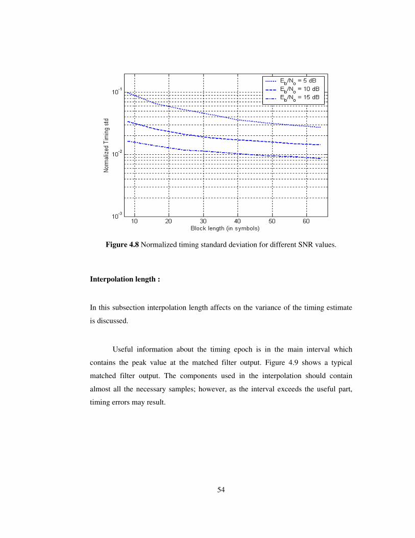
Observation interval:
The final accuracy is limited by the variance of the timing estimate. The primary
factor in obtaining a low variance of the timing estimate is the length of the
observation interval. The observation interval refers to the block length 0L used in
the correlation which can be defined as the number of the symbols used in timing
recovery, i.e., TLT 00 = . Figure 4.8 gives the relation of the variance to the block
length for different SNR. As is seen, the block length of 32 symbols is a good choice
even for low SNR values. Considering the moderate SNR values timing recovery can
also be performed satisfactorily for smaller 0L values.
54
Figure 4.8 Normalized timing standard deviation for different SNR values.
Interpolation length :
In this subsection interpolation length affects on the variance of the timing estimate
is discussed.
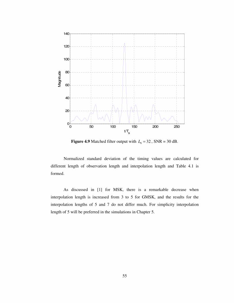
Useful information about the timing epoch is in the main interval which
contains the peak value at the matched filter output. Figure 4.9 shows a typical
matched filter output. The components used in the interpolation should contain
almost all the necessary samples; however, as the interval exceeds the useful part,
timing errors may result.
55
0 50 100 150 200 2500
20
40
60
80
100
120
140
t/Ts
Magnitude
Figure 4.9 Matched filter output with 0 32L = , SNR = 30 dB.
Normalized standard deviation of the timing values are calculated for
different length of observation length and interpolation length and Table 4.1 is
formed.
As discussed in [1] for MSK, there is a remarkable decrease when
interpolation length is increased from 3 to 5 for GMSK, and the results for the
interpolation lengths of 5 and 7 do not differ much. For simplicity interpolation
length of 5 will be preferred in the simulations in Chapter 5.
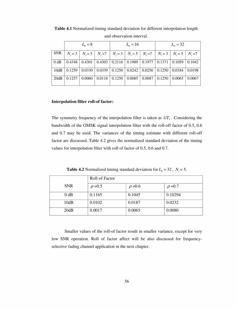
56
Table 4.1 Normalized timing standard deviation for different interpolation length
and observation interval.
0 8L = 0 16L = 0 32L =
SNR iN = 3 iN = 5 iN =7 iN = 3 iN = 5 iN =7 iN = 3 iN = 5 iN =7
0 dB 0.4348 0.4301 0.4303 0.2116 0.1989 0.1977 0.1371 0.1059 0.1042
10dB 0.1259 0.0330 0.0339 0.1250 0.0242 0.0256 0.1250 0.0184 0.0198
20dB 0.1257 0.0060 0.0118 0.1250 0.0085 0.0087 0.1250 0.0065 0.0067
Interpolation filter roll-of factor:
The symmetry frequency of the interpolation filter is taken as 1/Ts . Considering the
bandwidth of the GMSK signal interpolation filter with the roll-off factor of 0.5, 0.6
and 0.7 may be used. The variances of the timing estimate with different roll-off
factor are discussed. Table 4.2 gives the normalized standard deviation of the timing
values for interpolation filter with roll of factor of 0.5, 0.6 and 0.7.
Table 4.2 Normalized timing standard deviation for 0 32L = , iN = 5.
Roll-of Factor
SNR ρ =0.5 ρ =0.6 ρ =0.7
0 dB 0.1165 0.1045 0.10294
10dB 0.0102 0.0187 0.0232
20dB 0.0017 0.0065 0.0080
Smaller values of the roll-of factor result in smaller variance, except for very
low SNR operation. Roll of factor affect will be also discussed for frequency-
selective fading channel application in the next chapter.
57
CHAPTER 5
SIMULATION AND RESULTS
5.1 INTRODUCTION
The proposed decision-directed symbol synchronizer model has been developed in
MATLAB. Although MATLAB is based on discrete time signals, the continuous-
time signals are represented by their discrete samples taken at a rate much greater
than the Nyquist rate for a proper simulation.
In this chapter, firstly the model of the simulated system is presented. Next,
several properties of the GMSK modulated signal, the channel model and channel tap
generation process and methods of construction on the matched filter are discussed.
Performance of the symbol synchronizer in AWGN channel is compared with
MCRB for different observation intervals. Finally, the tracking performance of the
synchronizer is compared with Mazo criterion.
5.2 SIMULATION MODEL OF THE COMMUNICATION SYSTEM
The signal processing in the simulations is realized in baseband. The general
simulated diagram is shown in Figure 5.1.
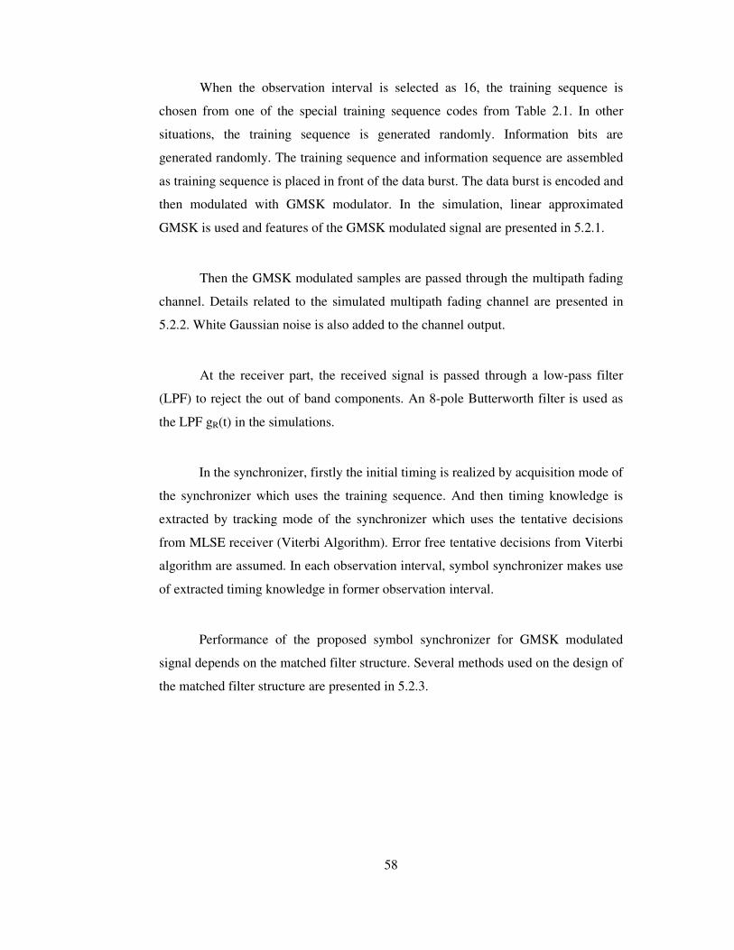
58
When the observation interval is selected as 16, the training sequence is
chosen from one of the special training sequence codes from Table 2.1. In other
situations, the training sequence is generated randomly. Information bits are
generated randomly. The training sequence and information sequence are assembled
as training sequence is placed in front of the data burst. The data burst is encoded and
then modulated with GMSK modulator. In the simulation, linear approximated
GMSK is used and features of the GMSK modulated signal are presented in 5.2.1.
Then the GMSK modulated samples are passed through the multipath fading
channel. Details related to the simulated multipath fading channel are presented in
5.2.2. White Gaussian noise is also added to the channel output.
At the receiver part, the received signal is passed through a low-pass filter
(LPF) to reject the out of band components. An 8-pole Butterworth filter is used as
the LPF gR(t) in the simulations.
In the synchronizer, firstly the initial timing is realized by acquisition mode of
the synchronizer which uses the training sequence. And then timing knowledge is
extracted by tracking mode of the synchronizer which uses the tentative decisions
from MLSE receiver (Viterbi Algorithm). Error free tentative decisions from Viterbi
algorithm are assumed. In each observation interval, symbol synchronizer makes use
of extracted timing knowledge in former observation interval.
Performance of the proposed symbol synchronizer for GMSK modulated
signal depends on the matched filter structure. Several methods used on the design of
the matched filter structure are presented in 5.2.3.
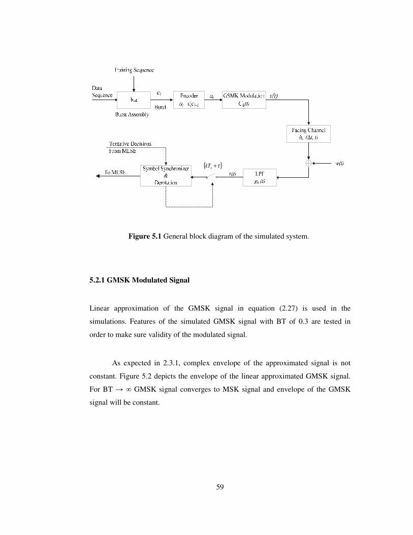
59
{ }τ+skT
Figure 5.1 General block diagram of the simulated system.
5.2.1 GMSK Modulated Signal
Linear approximation of the GMSK signal in equation (2.27) is used in the
simulations. Features of the simulated GMSK signal with BT of 0.3 are tested in
order to make sure validity of the modulated signal.
As expected in 2.3.1, complex envelope of the approximated signal is not
constant. Figure 5.2 depicts the envelope of the linear approximated GMSK signal.
For BT → ∞ GMSK signal converges to MSK signal and envelope of the GMSK
signal will be constant.
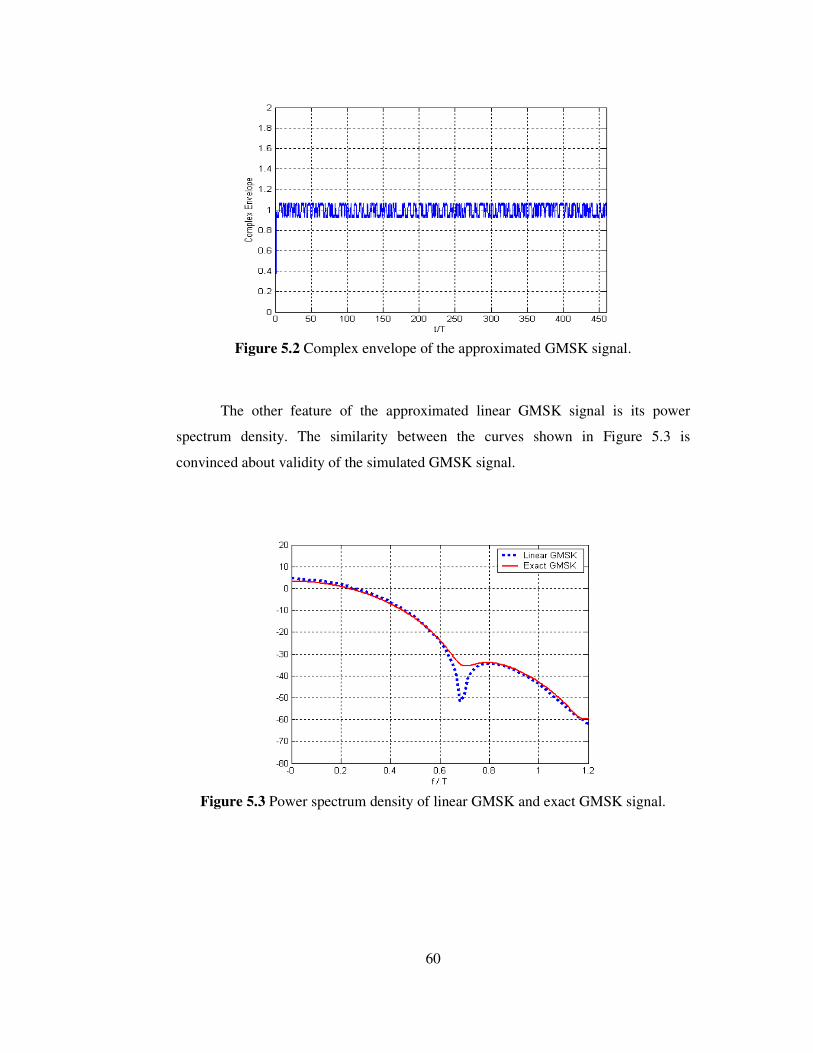
60
Figure 5.2 Complex envelope of the approximated GMSK signal.
The other feature of the approximated linear GMSK signal is its power
spectrum density. The similarity between the curves shown in Figure 5.3 is
convinced about validity of the simulated GMSK signal.
Figure 5.3 Power spectrum density of linear GMSK and exact GMSK signal.
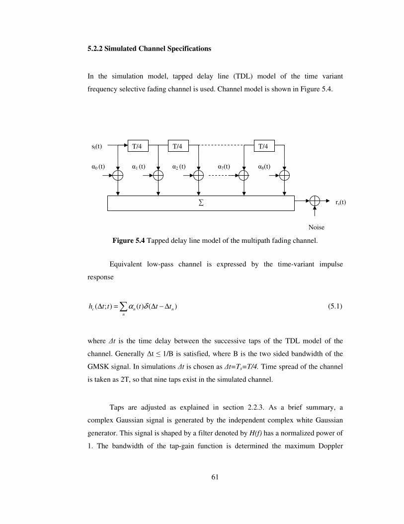
61
5.2.2 Simulated Channel Specifications
In the simulation model, tapped delay line (TDL) model of the time variant
frequency selective fading channel is used. Channel model is shown in Figure 5.4.
Figure 5.4 Tapped delay line model of the multipath fading channel.
Equivalent low-pass channel is expressed by the time-variant impulse
response
( ; ) ( ) ( )c n n
n
h t t t t tα δ∆ = ∆ − ∆∑ (5.1)
where ∆t is the time delay between the successive taps of the TDL model of the
channel. Generally ∆t ≤ 1/B is satisfied, where B is the two sided bandwidth of the
GMSK signal. In simulations ∆t is chosen as ∆t=Ts=T/4. Time spread of the channel
is taken as 2T, so that nine taps exist in the simulated channel.
Taps are adjusted as explained in section 2.2.3. As a brief summary, a
complex Gaussian signal is generated by the independent complex white Gaussian
generator. This signal is shaped by a filter denoted by H(f) has a normalized power of
1. The bandwidth of the tap-gain function is determined the maximum Doppler
T/4 T/4 T/4
∑
α0 (t) α1 (t) α2 (t) α7(t) α8(t)
sl(t)
Noise
rs(t)
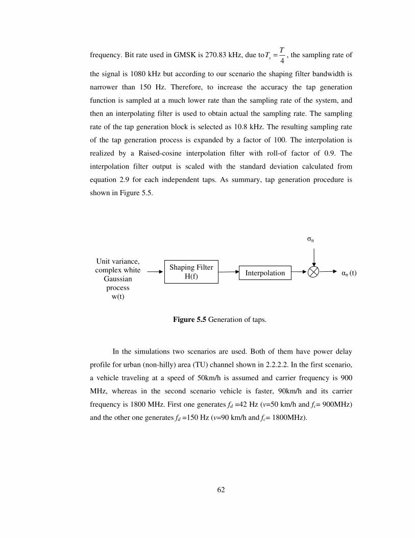
62
frequency. Bit rate used in GMSK is 270.83 kHz, due to4s
TT = , the sampling rate of
the signal is 1080 kHz but according to our scenario the shaping filter bandwidth is
narrower than 150 Hz. Therefore, to increase the accuracy the tap generation
function is sampled at a much lower rate than the sampling rate of the system, and
then an interpolating filter is used to obtain actual the sampling rate. The sampling
rate of the tap generation block is selected as 10.8 kHz. The resulting sampling rate
of the tap generation process is expanded by a factor of 100. The interpolation is
realized by a Raised-cosine interpolation filter with roll-of factor of 0.9. The
interpolation filter output is scaled with the standard deviation calculated from
equation 2.9 for each independent taps. As summary, tap generation procedure is
shown in Figure 5.5.
Figure 5.5 Generation of taps.
In the simulations two scenarios are used. Both of them have power delay
profile for urban (non-hilly) area (TU) channel shown in 2.2.2.2. In the first scenario,
a vehicle traveling at a speed of 50km/h is assumed and carrier frequency is 900
MHz, whereas in the second scenario vehicle is faster, 90km/h and its carrier
frequency is 1800 MHz. First one generates fd =42 Hz (v=50 km/h and fc= 900MHz)
and the other one generates fd =150 Hz (v=90 km/h and fc= 1800MHz).
Unit variance, complex white
Gaussian process
w(t)
Shaping Filter H(f) Interpolation
σn
αn (t)

63
5.2.3 Methods on the Matched Filter
The conclusive aim of a symbol synchronizer is to estimate the most likely value of
the timing epoch. In section 4.3.1 the correlation (matched filter) method was
discussed. The estimation of timing epoch is obtained by received signal passed
through the filter, which is matched to the reference signal over the observation
interval ( 0L ). This section presents two methods, called “Method A” and “Method
B”, on construction of the matched filter in other words the reference signal.
As explained in 4.3.1, in the acquisition mode a GMSK modulated signal
with the training sequence known by the receiver is used and in the tracking mode a
GMSK modulated signal with the tentative decisions, coming from MLSE receiver is
used. For the GMSK signal with BT=0.3, pulse shaping function g(t) in Figure 2.8
spans a time interval of approximately 4 symbol durations. Due to this, for the each
observation interval the GMSK modulated signal spans a time interval of 3 symbol
durations through the next observation interval. The last 3 symbol durations of the
modulated signal is called as “tail”. For each observation interval GMSK modulated
signal denotes as )(tsi . Beginning and ending points of the )(tsi ’s are shown in
Figure 5.6.
Method A constructs the reference signal by adding the first interval of 0L
symbol duration of the GMSK modulated signal of the currently observation interval
and last interval of 3 symbol duration of GMSK modulated signal from the previous
observation interval. Figure 5.7 depicts construction of the reference signal, ( )ir t by
Method A.
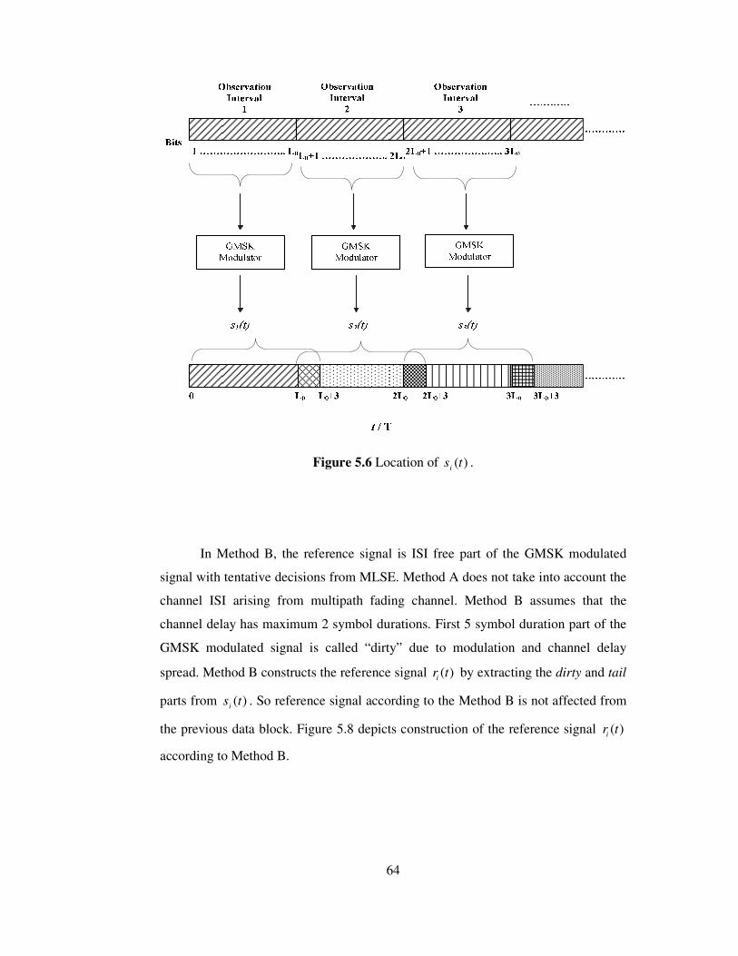
64
Figure 5.6 Location of )(tsi
.
In Method B, the reference signal is ISI free part of the GMSK modulated
signal with tentative decisions from MLSE. Method A does not take into account the
channel ISI arising from multipath fading channel. Method B assumes that the
channel delay has maximum 2 symbol durations. First 5 symbol duration part of the
GMSK modulated signal is called “dirty” due to modulation and channel delay
spread. Method B constructs the reference signal ( )ir t by extracting the dirty and tail
parts from )(tsi . So reference signal according to the Method B is not affected from
the previous data block. Figure 5.8 depicts construction of the reference signal ( )ir t
according to Method B.

65
Figure 5.7 Construction of the reference signal by Method A.
Figure 5.8 Construction of the reference signal by Method B.
Comparisons of Methods A and B are obtained by simulations. Figure 5.9 –
Figure 5.12 show the results pertaining to timing estimates using Method A and B.
under the effects of the multipath fading channels. The performance is given for
block length of oL = 16 or oL = 32. In order to illustrate effect of the fast variations,
two channel scenarios are used as explained before. Interpolation is performed within
an interval of iN = 5, and roll-off factor of 0.6.
As seen from the figures the curves are very close to distinguish the
differences thus an rms error is calculated for each situation. The rms error is defined
as;
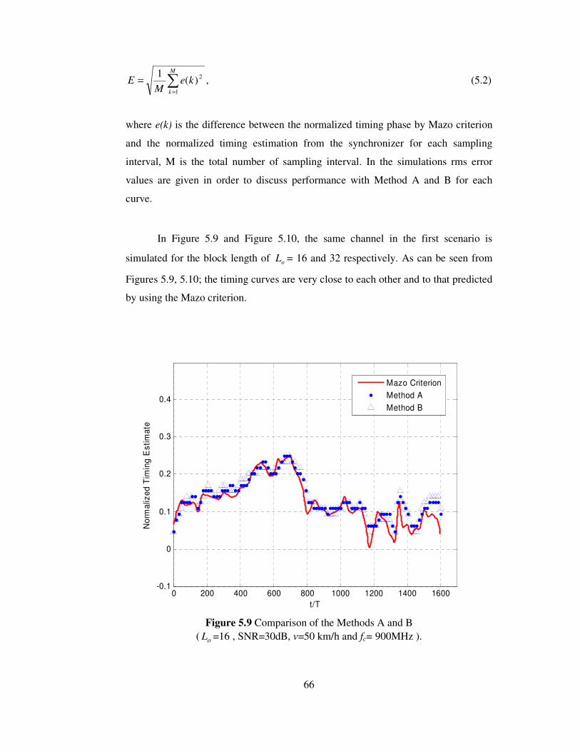
66
∑=
=M
k
keM
E1
2)(1
, (5.2)
where e(k) is the difference between the normalized timing phase by Mazo criterion
and the normalized timing estimation from the synchronizer for each sampling
interval, M is the total number of sampling interval. In the simulations rms error
values are given in order to discuss performance with Method A and B for each
curve.
In Figure 5.9 and Figure 5.10, the same channel in the first scenario is
simulated for the block length of oL = 16 and 32 respectively. As can be seen from
Figures 5.9, 5.10; the timing curves are very close to each other and to that predicted
by using the Mazo criterion.
0 200 400 600 800 1000 1200 1400 1600-0.1
0
0.1
0.2
0.3
0.4
t/T
No
rma
lize
d T
imin
g E
sti
ma
te
Mazo Criterion
Method A
Method B
Figure 5.9 Comparison of the Methods A and B
( oL =16 , SNR=30dB, v=50 km/h and fc= 900MHz ).
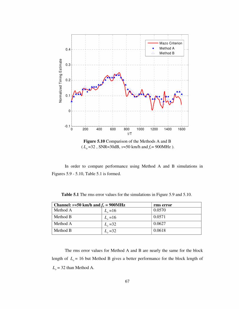
67
0 200 400 600 800 1000 1200 1400 1600-0.1
0
0.1
0.2
0.3
0.4
t/T
No
rma
lize
d T
imin
g E
sti
ma
te
Mazo Criterion
Method A
Method B
Figure 5.10 Comparison of the Methods A and B
( oL =32 , SNR=30dB, v=50 km/h and fc= 900MHz ).
In order to compare performance using Method A and B simulations in
Figures 5.9 - 5.10, Table 5.1 is formed.
Table 5.1 The rms error values for the simulations in Figure 5.9 and 5.10.
Channel: v=50 km/h and fc = 900MHz rms error Method A
oL =16 0.0570
Method B oL =16 0.0571
Method A oL =32 0.0627
Method B oL =32 0.0618
The rms error values for Method A and B are nearly the same for the block
length of oL = 16 but Method B gives a better performance for the block length of
oL = 32 than Method A.
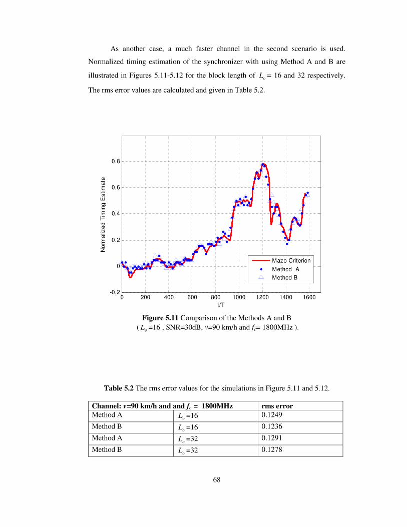
68
As another case, a much faster channel in the second scenario is used.
Normalized timing estimation of the synchronizer with using Method A and B are
illustrated in Figures 5.11-5.12 for the block length of oL = 16 and 32 respectively.
The rms error values are calculated and given in Table 5.2.
0 200 400 600 800 1000 1200 1400 1600-0.2
0
0.2
0.4
0.6
0.8
t/T
No
rma
lize
d T
imin
g E
sti
ma
te
Mazo Criterion
Method A
Method B
Figure 5.11 Comparison of the Methods A and B
( oL =16 , SNR=30dB, v=90 km/h and fc= 1800MHz ).
Table 5.2 The rms error values for the simulations in Figure 5.11 and 5.12.
Channel: v=90 km/h and and fc = 1800MHz rms error Method A
oL =16 0.1249
Method B oL =16 0.1236
Method A oL =32 0.1291
Method B oL =32 0.1278
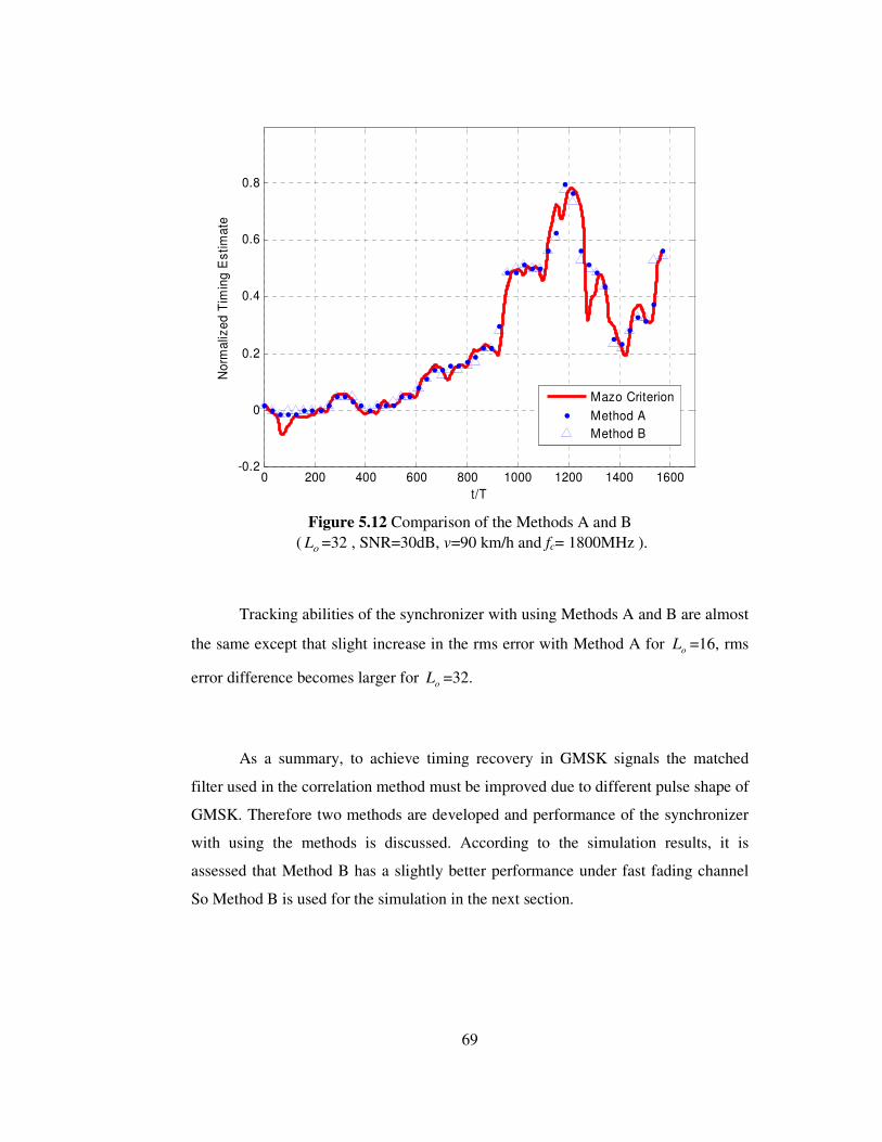
69
0 200 400 600 800 1000 1200 1400 1600-0.2
0
0.2
0.4
0.6
0.8
t/T
No
rma
lize
d T
imin
g E
sti
ma
te
Mazo Criterion
Method A
Method B
Figure 5.12 Comparison of the Methods A and B
( oL =32 , SNR=30dB, v=90 km/h and fc= 1800MHz ).
Tracking abilities of the synchronizer with using Methods A and B are almost
the same except that slight increase in the rms error with Method A for oL =16, rms
error difference becomes larger for oL =32.
As a summary, to achieve timing recovery in GMSK signals the matched
filter used in the correlation method must be improved due to different pulse shape of
GMSK. Therefore two methods are developed and performance of the synchronizer
with using the methods is discussed. According to the simulation results, it is
assessed that Method B has a slightly better performance under fast fading channel
So Method B is used for the simulation in the next section.
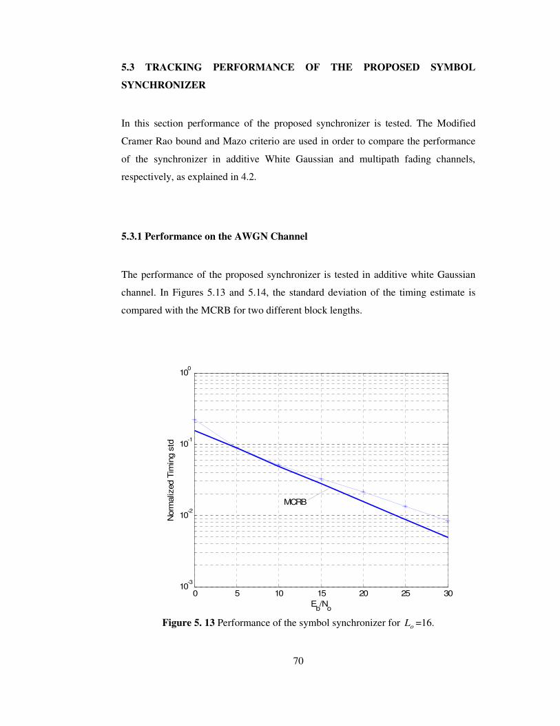
70
5.3 TRACKING PERFORMANCE OF THE PROPOSED SYMBOL
SYNCHRONIZER
In this section performance of the proposed synchronizer is tested. The Modified
Cramer Rao bound and Mazo criterio are used in order to compare the performance
of the synchronizer in additive White Gaussian and multipath fading channels,
respectively, as explained in 4.2.
5.3.1 Performance on the AWGN Channel
The performance of the proposed synchronizer is tested in additive white Gaussian
channel. In Figures 5.13 and 5.14, the standard deviation of the timing estimate is
compared with the MCRB for two different block lengths.
0 5 10 15 20 25 3010
-3
10-2
10-1
100
Eb/N
o
Norm
aliz
ed T
imin
g s
td
MCRB
Figure 5. 13 Performance of the symbol synchronizer for oL =16.
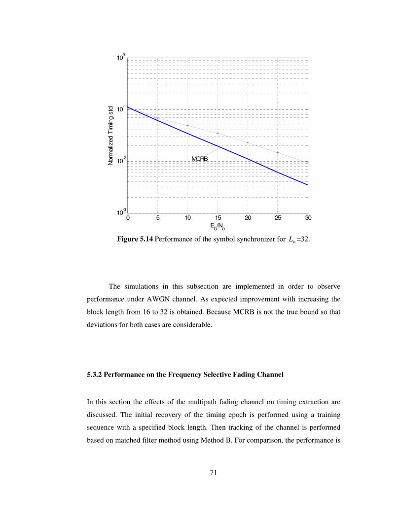
71
0 5 10 15 20 25 3010
-3
10-2
10-1
100
Eb/N
o
Norm
aliz
ed T
imin
g s
td
MCRB
Figure 5.14 Performance of the symbol synchronizer for oL =32.
The simulations in this subsection are implemented in order to observe
performance under AWGN channel. As expected improvement with increasing the
block length from 16 to 32 is obtained. Because MCRB is not the true bound so that
deviations for both cases are considerable.
5.3.2 Performance on the Frequency Selective Fading Channel
In this section the effects of the multipath fading channel on timing extraction are
discussed. The initial recovery of the timing epoch is performed using a training
sequence with a specified block length. Then tracking of the channel is performed
based on matched filter method using Method B. For comparison, the performance is

72
given for different values of the parameters; observation interval, SNR and roll of
factor of the interpolation filter.
Firstly, the tracking performance of the proposed timing recovery scheme is
tested for the first channel condition at 30 dB SNR for the block length of oL = 16,
32 and 64. Figure 5.15 shows the tracking ability for the performance for the block
length of oL =16 and 32. Simulation results are very similar to that obtained from the
Mazo criterion. Figure 5.16 depicts a comparison of the performances for block
lengths of oL =16 and 64. As seen from the figure, the synchronizer for the one with
block length of oL =64 can not track the channel variations as well as for the block
length of oL =16. The rms error values for the simulations in Figure 5.15 and 5.16
are given in Table 5.3.
Table 5.3 The rms error values for the simulations in Figure 5.15 and 5.16.
Channel: v=50 km/h and fc = 900MHz, SNR=30dB, ρ = 0.6, Method B
Block Length ( oL ) RMS Error
oL =16 0.0571
oL =32 0.0618
oL =64 0.0688
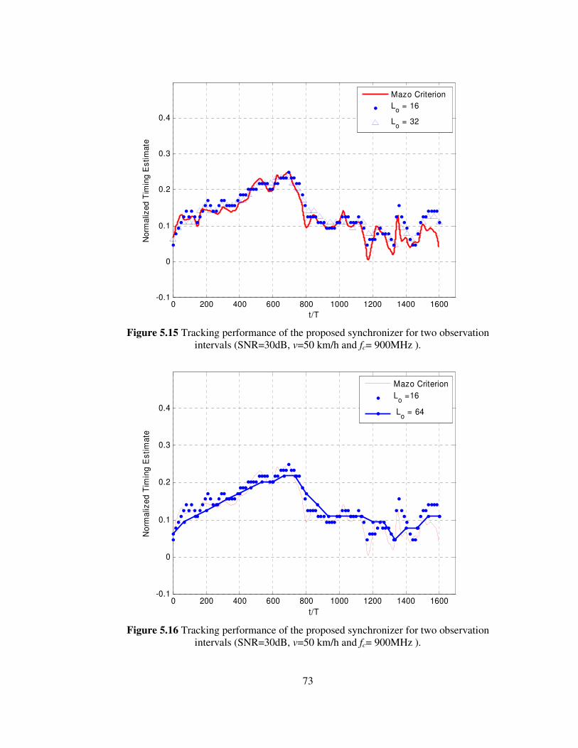
73
0 200 400 600 800 1000 1200 1400 1600-0.1
0
0.1
0.2
0.3
0.4
t/T
No
rma
lized
Tim
ing
Es
tim
ate
Mazo Criterion
Lo = 16
Lo = 32
Figure 5.15 Tracking performance of the proposed synchronizer for two observation
intervals (SNR=30dB, v=50 km/h and fc= 900MHz ).
0 200 400 600 800 1000 1200 1400 1600-0.1
0
0.1
0.2
0.3
0.4
t/T
No
rma
lize
d T
imin
g E
sti
ma
te
Mazo Criterion
Lo =16
Lo = 64
Figure 5.16 Tracking performance of the proposed synchronizer for two observation
intervals (SNR=30dB, v=50 km/h and fc= 900MHz ).
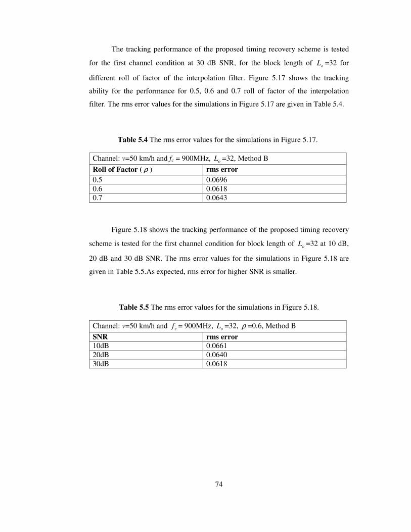
74
The tracking performance of the proposed timing recovery scheme is tested
for the first channel condition at 30 dB SNR, for the block length of oL =32 for
different roll of factor of the interpolation filter. Figure 5.17 shows the tracking
ability for the performance for 0.5, 0.6 and 0.7 roll of factor of the interpolation
filter. The rms error values for the simulations in Figure 5.17 are given in Table 5.4.
Table 5.4 The rms error values for the simulations in Figure 5.17.
Channel: v=50 km/h and fc = 900MHz, oL =32, Method B
Roll of Factor ( ρ ) rms error
0.5 0.0696 0.6 0.0618 0.7 0.0643
Figure 5.18 shows the tracking performance of the proposed timing recovery
scheme is tested for the first channel condition for block length of oL =32 at 10 dB,
20 dB and 30 dB SNR. The rms error values for the simulations in Figure 5.18 are
given in Table 5.5.As expected, rms error for higher SNR is smaller.
Table 5.5 The rms error values for the simulations in Figure 5.18.
Channel: v=50 km/h and cf = 900MHz, oL =32, ρ =0.6, Method B
SNR rms error 10dB 0.0661 20dB 0.0640 30dB 0.0618
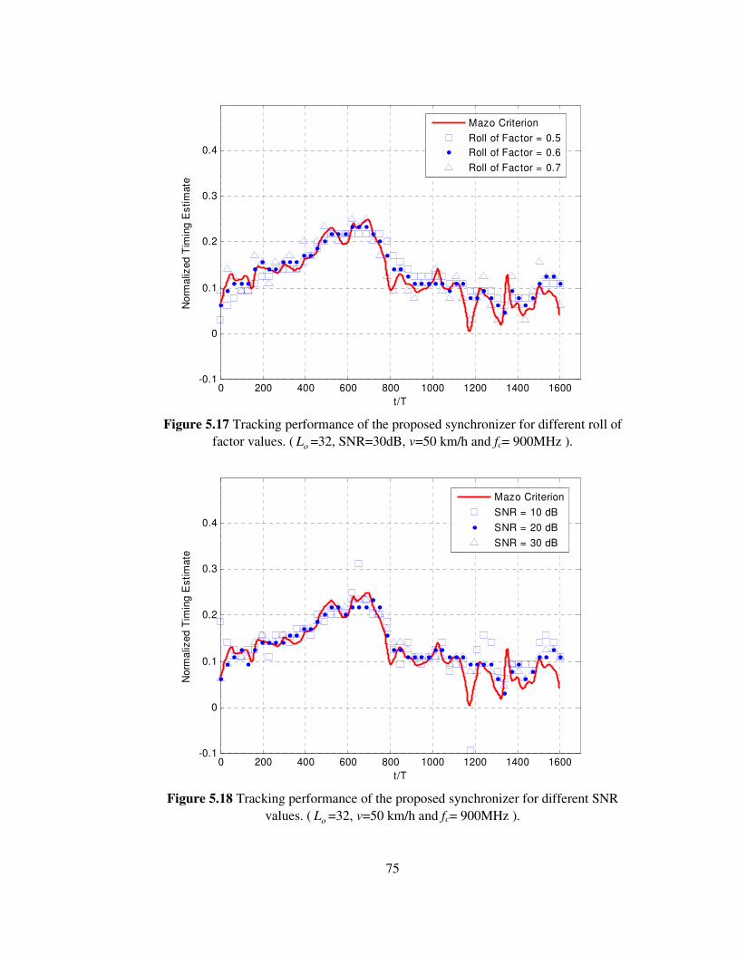
75
0 200 400 600 800 1000 1200 1400 1600-0.1
0
0.1
0.2
0.3
0.4
t/T
No
rma
lized
Tim
ing
Es
tim
ate
Mazo Criterion
Roll of Factor = 0.5
Roll of Factor = 0.6
Roll of Factor = 0.7
Figure 5.17 Tracking performance of the proposed synchronizer for different roll of
factor values. ( oL =32, SNR=30dB, v=50 km/h and fc= 900MHz ).
0 200 400 600 800 1000 1200 1400 1600-0.1
0
0.1
0.2
0.3
0.4
t/T
No
rma
lize
d T
imin
g E
sti
ma
te
Mazo Criterion
SNR = 10 dB
SNR = 20 dB
SNR = 30 dB
Figure 5.18 Tracking performance of the proposed synchronizer for different SNR
values. ( oL =32, v=50 km/h and fc= 900MHz ).

76
The simulations for the first channel are repeated for a faster channel in the
second scenario. The tracking performance of the proposed timing recovery scheme
is tested at 30 dB SNR for block length of oL =8, 16, 32 and 64. Figure 5.19 shows
the tracking ability for block lengths of oL =16 and 32. Simulation results are very
similar to the values obtained from the Mazo criterion. Figure 5.20 depicts a
comparison of the performances for block lengths of oL =16 and 64. Figure 5.20
clearly shows the insufficiency of the synchronizer for block length of oL =64 can
not track the channel variations whereas the synchronizer for the block length of
oL = 16 can track the channel variation successfully.
The rms error values for the simulations in Figure 5.19 and 5.20 are given in
Table 5.6. As expected, the rms error values are worse than error figures of the first
channel. Table 5.6 shows the block length of oL = 8 and
oL = 64 are not good
candidates. Timing estimate of the synchronizer for the block length of oL =64 is too
sparsely updated that it can not track the channel variations. For the synchronizer
using a block length of oL =8, observation interval is too short to provide sufficient
noise suppression.
Table 5.6 The rms error values for the simulations in Figure 5.19 and 5.20.
Channel: v=90 km/h and cf = 1800MHz, SNR=30dB, ρ =0.6, Method B
oL rms error
oL =8 0.1414
oL =16 0.1236
oL =32 0.1278
oL =64 0.1421
As a result of Table 5.3 and 5.6, observation interval oL =16 and oL =32 are
selectable.

77
0 200 400 600 800 1000 1200 1400 1600-0.2
0
0.2
0.4
0.6
0.8
t/T
Norm
aliz
ed T
imin
g E
stim
ate
Mazo Criterion
Lo = 16
Lo = 32
Figure 5.19 Tracking performance of the proposed synchronizer for two observation intervals (SNR=30dB, v=90 km/h and fc= 1800MHz ).
0 200 400 600 800 1000 1200 1400 1600-0.2
0
0.2
0.4
0.6
0.8
t/T
Norm
aliz
ed T
imin
g E
stim
ate
Mazo Criterion
Lo = 16
Lo = 64
Figure 5.20 Tracking performance of the proposed synchronizer for two observation intervals (SNR=30dB, v=90 km/h and fc= 1800MHz ).
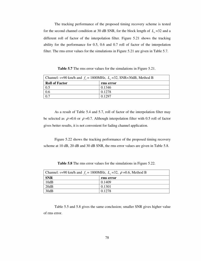
78
The tracking performance of the proposed timing recovery scheme is tested
for the second channel condition at 30 dB SNR, for the block length of oL =32 and a
different roll of factor of the interpolation filter. Figure 5.21 shows the tracking
ability for the performance for 0.5, 0.6 and 0.7 roll of factor of the interpolation
filter. The rms error values for the simulations in Figure 5.21 are given in Table 5.7.
Table 5.7 The rms error values for the simulations in Figure 5.21.
Channel: v=90 km/h and cf = 1800MHz, oL =32, SNR=30dB, Method B
Roll of Factor rms error 0.5 0.1346 0.6 0.1278 0.7 0.1297
As a result of Table 5.4 and 5.7, roll of factor of the interpolation filter may
be selected as ρ =0.6 or ρ =0.7. Although interpolation filter with 0.5 roll of factor
gives better results, it is not convenient for fading channel application.
Figure 5.22 shows the tracking performance of the proposed timing recovery
scheme at 10 dB, 20 dB and 30 dB SNR, the rms error values are given in Table 5.8.
Table 5.8 The rms error values for the simulations in Figure 5.22.
Channel: v=90 km/h and cf = 1800MHz, oL =32, ρ =0.6, Method B
SNR rms error 10dB 0.1409 20dB 0.1301 30dB 0.1278
Table 5.5 and 5.8 gives the same conclusion; smaller SNR gives higher value
of rms error.
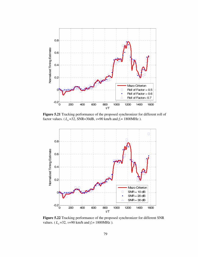
79
0 200 400 600 800 1000 1200 1400 1600-0.2
0
0.2
0.4
0.6
0.8
t/T
Norm
aliz
ed T
imin
g E
stim
ate
Mazo Criterion
Roll of Factor = 0.5
Roll of Factor = 0.6
Roll of Factor= 0.7
Figure 5.21 Tracking performance of the proposed synchronizer for different roll of factor values. ( oL =32, SNR=30dB, v=90 km/h and fc= 1800MHz ).
0 200 400 600 800 1000 1200 1400 1600-0.2
0
0.2
0.4
0.6
0.8
t/T
Norm
aliz
ed T
imin
g E
stim
ate
Mazo Criterion
SNR = 10 dB
SNR = 20 dB
SNR = 30 dB
Figure 5.22 Tracking performance of the proposed synchronizer for different SNR values. ( oL =32, v=90 km/h and fc= 1800MHz ).

80
CHAPTER 6
CONCLUSION
Throughout this study, it has been noticed that although there are plenty of research
studies on the area of symbol synchronization for CPM signals, there are still issues
that are to be investigated in the frequency selective fading channel transmission
area.
In this study, symbol timing recovery for CPM signals over multipath fading
channel was examined by employing GMSK signal. The reason of choosing GMSK
among the CPM family is its common use within digital communication systems like
GSM and DECT.
In the GSM system, specific training sequences which have good
crosscorrelation properties are used for channel identification. In this study, the
channel identification solution based on correlation method was reviewed and the
training sequences were presented. In order to take advantage of the good correlation
property, the training sequences were used throughout the initial timing acquisition
in simulations.
As it is mentioned in the literature, approximation of GMSK modulation as a
linear modulation is necessary to enable the use of MLSE method in receiver.
Consequently, the linearly approximated GMSK was reviewed, power spectrum
density and waveform envelope of the linear GMSK signal were examined and

81
observed as expected. Time varying multipath fading channel with TU delay power
profile has been simulated.
The performance of the recovery scheme in MSK over multipath fading
channel was examined in [1] by using the proposed timing recovery scheme which
was based on correlation (matched filter) method by using the samples of the
received signal. The same matched filter could not be used for both MSK and GMSK
modulation scheme due to different spanning duration of their pulse shapes. As a
result, two methods; “Method A” and “Method B” were developed in order to
construct the matched filter for the application on GMSK signals.
Tracking ability of the synchronizer by using both methods was simulated. In
order to compare these methods rms error values were calculated by using Mazo
criterion which is an important tool in the context. According to the simulation
figures, it was observed that both methods could track channel variation successfully.
However, it was assessed that Method B has a slightly better performance than
Method A especially under fast fading channel conditions with respect to rms error
values. Consequently, Method B was used for the simulations throughout the study.
Precise timing estimation was achieved by employing interpolation and
iterative maximum search process. Moreover, interpolation filter structure was
examined with simulations. The initial timing information was acquired by using a
training sequence, placed in front of the data burst. Tracking mode is performed by
tentative decisions from MLSE receiver in the proposed timing recovery [1].
However, in this study, tentative decisions were assumed to be error free and
tracking mode was performed by them. Furthermore, Mazo criterion was used as a
basis for the tracking performance of the proposed scheme.
Simulations were repeated for different value of parameters; length of
observation interval, roll of factor of interpolation filter and SNR. By investigating
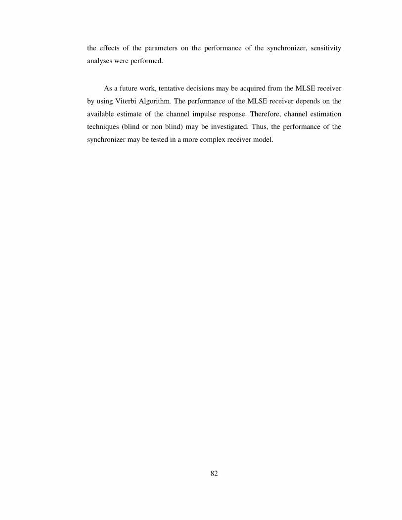
82
the effects of the parameters on the performance of the synchronizer, sensitivity
analyses were performed.
As a future work, tentative decisions may be acquired from the MLSE receiver
by using Viterbi Algorithm. The performance of the MLSE receiver depends on the
available estimate of the channel impulse response. Therefore, channel estimation
techniques (blind or non blind) may be investigated. Thus, the performance of the
synchronizer may be tested in a more complex receiver model.
83
REFERENCES
[1] S. Sezginer, “Symbol Synchronization For MSK Signals Based On Matched Filtering,” M.Sc. Thesis, Electrical and Electronics Eng. Dept., Middle East Technical University, Ankara, September 2003.
[2] S. Sezginer, Y. Tanık, “An Improved Matched Filter Based Symbol Synchronizer For MSK Transmission Over Fading Multipath Channels,” IEEE Vehicular Technology Conference, vol. 3, pp. 1678 – 1682, Sept. 2004.
[3] J. G Proakis, “Digital Communications,” Singapore, McGraw-Hill, 1995.
[4] S. Eken, “A Study on GMSK Modulation And Channel Simulation,” M.Sc. Thesis, Electrical and Electronics Eng. Dept., Middle East Technical University, Ankara, Feb. 1994.
[5] M. C. Jeruchim, P. Balaban and K. S. Shanmugan, “Simulation of Communication Systems Modeling, Methodology, and Techniques,” New York, Second Ed., Kluwer Academic, 2002.
[6] J. Eberspacher, H-J Vögel, C. Bettstetter, “GSM Switching, Services and Protocols,” John-Wiley, Second Edition, 1999.
[7] P. A. Laurent, “Exact and Approximate Construction of Digital Phas Modulation by Superposition of Amplitude Modulated Pulses (AMP),” IEEE Trans. Commun., vol. Com-34, pp. 150-160, Feb. 1986.
[8] P. Jung, “Laurent’s representation of binary digital continuous phase modulated signals with modulation index 1/2 revisited,” IEEE Trans. Commun., vol. 42, pp. 221-224, 1994.
84
[9] A Wiesler, F. K. Jondral, “A software Radio For Second and Third Generation Mobile Systems ”, IEEE Trans. Commun., vol. Com-51, No 4, pp 738- 748 July 2002.
[10] A Wiesler, R. Machauer, F. Jondral, “Comparison of GMSK and Linear Approximated GMSK For Use In Software Radio”, IEEE, pp 557-560, 1998.
[11] B. Canpolat, “Design and Simulation of an Adaptive MLSE Receiver for GSM System,” M.Sc. Thesis, Electrical and Electronics Eng. Dept., Middle East Technical University, Ankara, Feb. 1994.
[12] A. Mehrotra, GSM System Engineering, Boston, Artech House, 1996.
[13] H. Meyr and G. Ascheid, Synchronization in Digital Communications, vol.1, New York: John Wiley & Sons, 1990.
[14] H. Meyr, M Moeneclaey, and S. A. Fechtel, Digital Communication, New York: McGraw-Hill, 1968.
[15] U. Mengali and A. N. D’Andrea, Synchronization Techniques for Digital Receivers, New York: Plenum Press, 1997.
[16] R. de Buda, ”Coherent Demodulation of Frequency Shift Keying with Low Deviation Ratio,” IEEE Trans. Commun., vol. COM-20, pp. 429-435, June 1972.
[17] T. Aulin and C. E. Sundberg, “Synchronization Properties of Continuous Phase Modulation,” in Proc. Int Conf. Commun., Philadelphia, PA, pp. D7.1.1-D7.1.7, June 1982.
[18] A. N. D’Andrea, U. Mengali, and R. Reggiannini, “Carrier Phase and Clock Recovery for Continuous Phase Modulated Signals,” IEEE Trans. Commun., vol. COM-35, pp. 1095-1101, Oct. 1987.
[19] J. Huber and W. Liu, “Data-Aided Synchronization of Coherent CPM Receivers,” IEEE Trans. Commun., vol. COM-40 pp. 178-189, Jan. 1992.
[20] R. Melhan, Y.E. Chen, and H. Meyr, “A Fully Digital Feedforward MSK Demodulator with Joint Frequency Offset and Symbol Timing Estimation for
85
Burst Mode Mobile Radio”, IEEE Trans. Veh. Techol., vol. VT-42 pp. 434-443, Nov. 1993.
[21] U. Lambrette and H. Meyr, “Two Timing Recovery Algorithms for MSK,” in Proc.ICC’94, New Orleans, LO, pp. 918-992, May 1994.
[22] M. Morelli and G. M. Vitetta, “Two Timing Recovery Algorithms for MSK,” in Proc. ICC’94, New Orleans, LO, pp. 1997-1999, Dec. 2000.
[23] F. Patenaude, J. H. Lodge, and P. A. Galko, “Symbol Timing Tracking for Continuous Phase Modulation over Fast Flat-Fading Channels,” IEEE Trans. Veh. Technol., vol. VT-40 pp. 615-626, Aug. 1991.
[24] L.E. Franks, “Carrier and Bit Synchronization in Data Communication- A Tutorial Review,” IEEE Trans. Commun., vol. COM-28, pp. 1107-1120, Aug. 1980.
[25] L. P. Sabel, “Maximum Likelihood Approach to Symbol Timing Recovery in Digital Communications,” Ph.D. Thesis, Sch. Of Elec. Eng. Univ. South Australia, South Australia, Oct. 1993.
[26] H.L. Van Trees, Detection, Estimation and Modulation Theory Part I, New York: John Wiley & Sons, 1968.
[27] K. H. Muller and M. Muller, “Timing Recovery in Digital synchronous Data Receivers,” IEEE Trans. Commun., vol. COM-24, pp. 516-531, May 1976.
[28] J. E. Mazo, “Optimum Timing Phase for an Infinite Equalizer,” Bell Syst, Tech. J., vol. 54, pp. 189-201, 1975.
[29] R. W. Lucky, J. Salz, and E. J. Weldon, Jr., Principals of Data Communication, New York: McGraw-Hill, 1968.
[30] A. V. Oppenheim and R. W: Schafer, Discrete-Time Signal Processing, Upper Saddle River, NJ: Prentice-Hall, 1999.
[31] A. N. D’Andrea, U. Mengali, and M. Morelli, “Symbol Timing Estimation with CPM Modulation,” IEEE Trans. Commun., vol. COM-44, pp. 1362-1372, Oct. 1996.

86
[32] R. Steele, Chin-Chun Lee, P. Gould, GSM, cdmaOne and 3G Systems, West Sussex, John Wiley & Sons ltd., 2001.
87
APPENDIX A
CPM SIGNALS
Continuous phase modulation (CPM) conserves and reduces signal energy and
bandwidth at the same time. CPM is a constant envelope, nonlinear modulation
method with memory. The constant envelope property of CPM schemes makes
possible to use non-linear amplifiers. The phase is a continuous function of time
since the data symbols modulate the instantaneous phase of the transmitted signal.
A.1 SIGNAL MODEL
The complex envelope of a CPM signal is given by [31]
));((2)( ταφθ −+= tis e
T
Ets , (A.1)
where Es is the energy per signaling interval, T is the symbol period, θ is carrier
phase, τ is timing epoch, α ={ α i } are data sequence from the alphabet {±1, ±3,…..,
±(M-1)} and φ (α,t) is the information-bearing phase:

88
∑ −=i
ii itqht )(2);( ταπαφ . (A.2)
The parameter hi is called the modulation index.. When hi =h for all i, the
modulation index is fixed for all symbols. When the modulation index varies from
one symbol to another, the CPM signal is called multi-h. q(t) is the phase pulse of the
modulator, which is related to the frequency pulse g(t) by
∫∞−
=t
dgtq ττ )()( , (A.3)
and is normalized in such a way that
1/ 2, t( )
0 , t<0
LTq t
≥=
. (A.4)
The phase pulse is nonzero in the interval t ∈ (0, LT), where L is an integer
called the correlation length. If L=1, the modulated signal is called full response
CPM. If L>1, the modulated signal is called partial response CPM. The CPM signal
has memory that is introduced through the phase continuity. For L>1, additional
memory is introduced in the CPM signal by the pulse g(t).
By choosing different frequency pulses and varying the parameters h and M,
a great variety of CPM schemes may be formed.
A.2 MINIMUM SHIFT KEYING AND GAUSSIAN MINIMUM SHIFT
KEYING
A subset of CPM signals is minimum shift keying (MSK) corresponds to
h=1/2, M=2 and a rectangular frequency pulse
89
1/ 2 , 0< t( )
0 , elsewhere
T Tg t
≤=
. (A.5)
MSK modulation is a constant envelope digital modulation. The spectrum of
MSK is quite large and substantial energy exists in the sidelobes.
The spectrum of an MSK modulated signal may be compressed by filtering
the modulating baseband pulses to produce much smoother changes in frequency,
thereby compressing the bandwidth of the modulated signal. The type of filter used
has a Gaussian impulse response and the resulting modulation scheme is called
Gaussian MSK (GMSK). The relative bandwidth of the Gaussian filter defines the
spectrum compression that is achieved, i.e. a smaller filter bandwidth results in a
narrower modulated spectrum. Unfortunately, the Gaussian filter also introduces ISI
whereby each modulation symbol spreads into adjacent symbols [32].
In this thesis, the emphasis is given on Gaussian MSK (GMSK), which is
used as the GSM modulation scheme. GMSK is obtained by letting h=1/2, M=2 and
g(t) is given by,
g(t)=h(t)* rect(t/T). (A.6)
Gaussian shaped impulse response, h(t) is given by;
2
2 2
1( ) exp
22
th t
TT σπσ
= −
, (A.7)
where
ln 2 / 2 BTσ π= (A.8)

90
here, B is the 3 dB bandwidth of the filter.
rect (t/T) is defined by;
1/ , t / 2( / )
0 , otherwise
T Trect t T
<=
, (A.9)
then,
1 2 ( / 2) 2 ( / 2)( )
2 ln 2 ln 2
B t T B t Tg t erf erf
T
π π − += − + −
, (A.10)
where
2
0
2( ) exp( )
x
erf x dυ υπ
= −∫ (A.11)
Figure A.1 Impulse Response of g(t)

91
The resulting impulse response g(t) is given in Fig A.1 for some values of
BT. Notice that with decreasing BT the impulse response becomes broader. For
BT → ∞ it converges to rect(.) function, also GMSK signal converges to MSK
signal. The Gaussian low-pass filtering has the effect of additional smoothing but
also of the broadening the impulse response g(t). This means that, the power
spectrum of the signal is made narrower, but on the other hand the individual impulse
responses are “smeared” across several bit durations, which leads to increase
intersymbol interference.
92
APPENDIX B
APPROXIMATION OF GMSK TO LINEAR QAM SIGNAL
The GMSK signal can be approximated to a linear QAM signal by adopting a
suitable pulse shape [4]. The pulse shape happens to be an approximately Gaussian
function spanning a time interval of approximately four symbol durations as will be
derived in this appendix.
The phase expression of GMSK signal is given as;
∑∫ −=∞− k
k
t
dkTgat ττπ
φ )(2
)( , (B.1)
which can also be expressed as;
∫∑−
∞−
=kTt
k
k dgat ττπ
φ )(2
)( , (B.2)
where ak’s are the differentially encoded bits in the form of ± 1, and g(t) is the
shaping function given as;
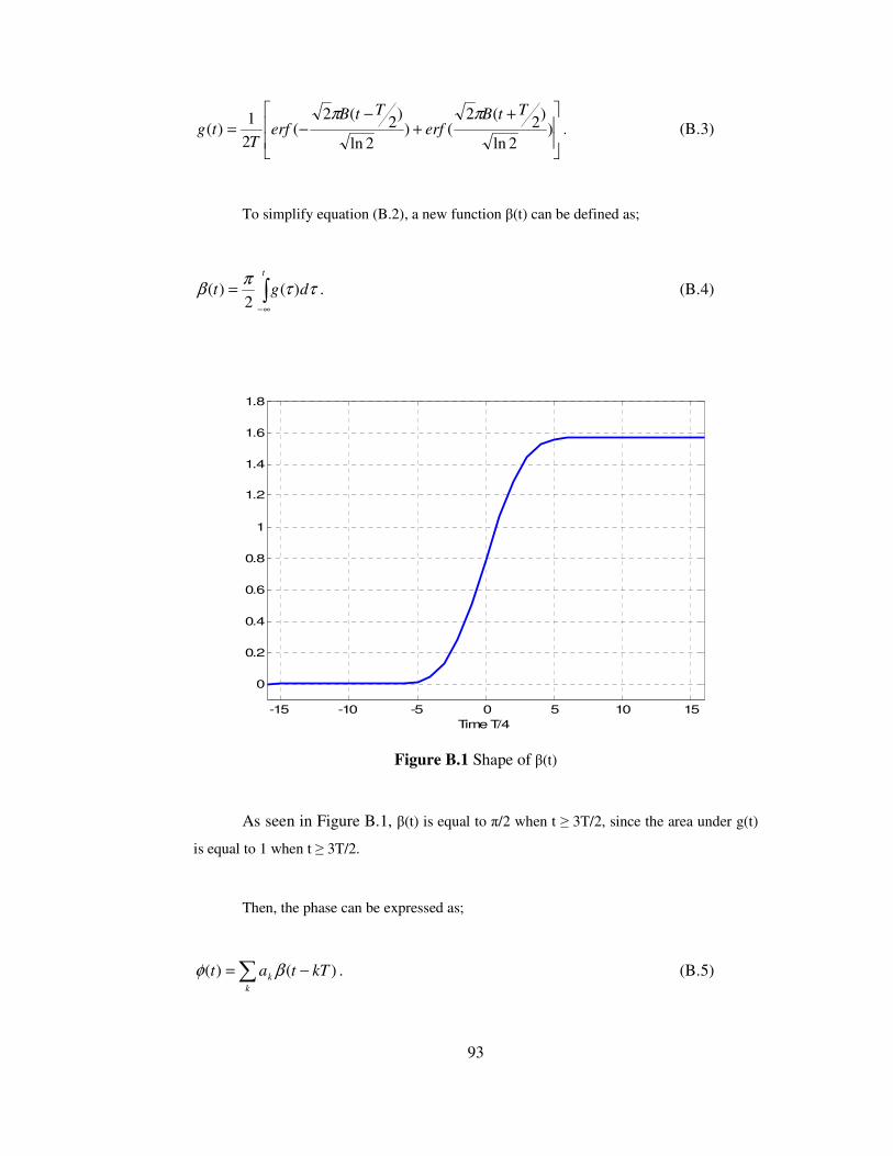
93
++
−−= )
2ln
)2(2()
2ln
)2(2(
2
1)(
TtBerf
TtBerf
Ttg
ππ. (B.3)
To simplify equation (B.2), a new function β(t) can be defined as;
∫∞−
=t
dgt ττπ
β )(2
)( . (B.4)
-15 -10 -5 0 5 10 15
0
0.2
0.4
0.6
0.8
1
1.2
1.4
1.6
1.8
Time T/4
Figure B.1 Shape of β(t)
As seen in Figure B.1, β(t) is equal to π/2 when t ≥ 3T/2, since the area under g(t)
is equal to 1 when t ≥ 3T/2.
Then, the phase can be expressed as;
)()( kTtatk
k −=∑ βφ . (B.5)

94
Thus, the baseband GMSK signal can be rewritten as;
sb(t)=exp j
−∑
k
k kTta )(β , (B.6)
Now consider the time interval (2n-1)T/2 ≤ t ≤ (2n+1)T/2. For this interval, if
k ≤ (n-2) then β(t-kT)= π/2 since in this case (t-kT) ≥ 3T/2. Therefore, the above equation
can be rewritten as;
sb(t)=exp j
−+− ∑∑
+
−=
−
−∞=
1
1
2
)()(n
nk
k
n
k
k kTtakTta ββ , (B.7)
and for the time interval (2n-1)T/2 ≤ t ≤ (2n+1)T/2 one can get;
sb(t)=exp j
∑
−
=
2
02
n
k
kaπ
exp j
−∑
+
−=
1
1
)(n
nk
k kTta β , (B.8)
sb(t)=exp j
∑
−
=
2
02
n
k
kaπ
[ ]1
1
exp j ( ( ) )n k
k
a t n k Tβ−=−
− −∏ , (B.9)
In the light of above equations, it can be shown that [4] the baseband GMSK
signal may be expressed as;
sb(t)=3 2
0 1
exp ( )2
N
n N i ki k
N k n i
j a a C t NTπ
α∞
−=−∞ = =−∞ =
− −
∑ ∑ ∑ ∑ , (B.10)
where,
001 =α 111 =α 021 =α 131 =α

95
002 =α 012 =α 122 =α 132 =α
and the functions Ck(t), k=0,1,2,3 are defined by;
C0(t) = [ ] [ ] [ ])(sin)(sin)(sin TttTt +− βββ 22
Tt
T≤≤
−
= [ ] [ ]
−−− )2(
2sin)(sin)(sin TttTt β
πββ
2
3
2
Tt
T≤≤
= [ ]
−−
−−− )2(
2sin)3(
2sin)(sin TtTtTt β
πβ
πβ
2
5
2
3 Tt
T≤≤
=
−−
−−
−− )2(
2sin)3(
2sin)4(
2sin TtTtTt β
πβ
πβ
π
2
7
2
5 Tt
T≤≤
= 0 elsewhere
(B.11)
C1(t) = [ ] [ ]
−+− )(
2sin)(sin)(sin tTtTt β
πββ
22
Tt
T≤≤
−
= [ ]
−
−−− )(
2sin)2(
2sin)(sin tTtTt β
πβ
πβ
2
3
2
Tt
T≤≤
= 0 elsewhere
(B.12)
C2(t) = [ ] [ ]
+−− )(
2sin)(sin)(sin TttTt β
πββ
22
Tt
T≤≤
−
= 0 elsewhere
(B.13)
C3(t) = [ ]
+−
−− )(
2sin)(
2sin)(sin TttTt β
πβ
πβ
22
Tt
T≤≤
−
= 0 elsewhere
(B.14)
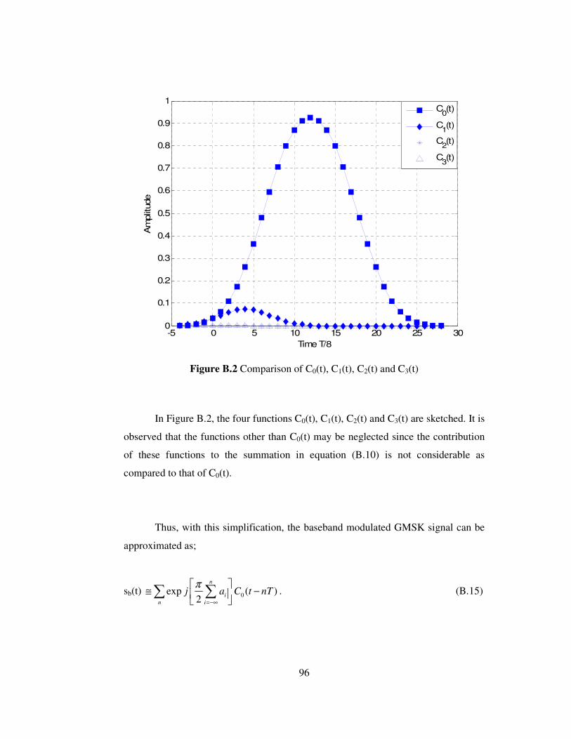
96
-5 0 5 10 15 20 25 300
0.1
0.2
0.3
0.4
0.5
0.6
0.7
0.8
0.9
1
Time T/8
Am
plit
ude
C0(t)
C1(t)
C2(t)
C3(t)
Figure B.2 Comparison of C0(t), C1(t), C2(t) and C3(t)
In Figure B.2, the four functions C0(t), C1(t), C2(t) and C3(t) are sketched. It is
observed that the functions other than C0(t) may be neglected since the contribution
of these functions to the summation in equation (B.10) is not considerable as
compared to that of C0(t).
Thus, with this simplification, the baseband modulated GMSK signal can be
approximated as;
sb(t) 0exp ( )2
n
i
n i
j a C t nTπ
=−∞
≅ −
∑ ∑ . (B.15)
Top Related