Download - Stochastic conjugate gradient method for least-square seismic inversion problems C… · · 2014-11-03Stochastic conjugate gradient method for least-square seismic inversion problems

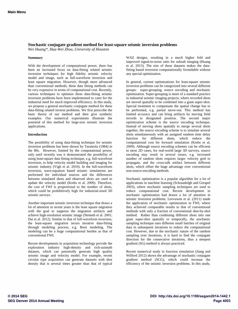
Stochastic conjugate gradient method for least-square seismic inversion problems Wei Huang*, Hua-Wei Zhou, University of Houston Summary With the development of computational power, there has been an increased focus on data-fitting related seismic inversion techniques for high fidelity seismic velocity model and image, such as full-waveform inversion and least square migration. However, though more advanced than conventional methods, these data fitting methods can be very expensive in terms of computational cost. Recently, various techniques to optimize these data-fitting seismic inversion problems have been implemented to cater for the industrial need for much improved efficiency. In this study, we propose a general stochastic conjugate method for these data-fitting related inverse problems. We first prescribe the basic theory of our method and then give synthetic examples. Our numerical experiments illustrate the potential of this method for large-size seismic inversion applications. Introduction The possibility of using data-fitting technique for seismic inversion problems has been shown by Tarantola (1984) in the 80s. However, limited by the computational power, only until recently was it demonstrated the possibility of using least-square data fitting technique, e.g. full-wavefrom inversion, to help velocity model building and imaging for seismic industry (Vigh et al. 2010). In the full-waveform inversion, wave-equation based seismic simulations are performed for individual sources and the differences between simulated shots and observed shots are used to update the velocity model (Krebs et al. 2009). Therefore, the cost of FWI is proportional to the number of shots, which could be prohibitively high for industrial-sized 3D seismic surveys. Another important seismic inversion technique that draws a lot of attention in recent years is the least square migration with the goal to suppress the migration artifacts and achieve high-resolution seismic image (Nemeth et al. 2001; Dai et al. 2012). Similar to that of full-waveform inversion, the least-square migration incurs iterative data-fitting through modeling process, e.g. Born modeling. The modeling can be a huge computational burden as that of conventional FWI. Recent developments in acquisition technology provide the exploration industry high-density and rich-azimuth datasets, which can potentially generate high quality seismic image and velocity model. For example, recent circular type acquisition can generate datasets with shot density that is several times greater than that of typical

WAZ designs, resulting in a much higher fold and improved signal-to-noise ratio for subsalt imaging (Huang et al. 2013). The size of these datasets makes the data-fitting based inversion computationally formidable without any special optimization. In general, current optimizations for least-square seismic inversion problems can be categorized into several different groups: super-grouping, source encoding and stochastic optimization. Super-grouping is more of a standard practice in industrial seismic imaging projects, where recorded shots are moved spatially to be combined into a giant super-shot. Special treatment to compensate the spatial change has to be performed, e.g. partial move-out. This method has limited accuracy and can bring artifacts by moving field records to designated position. The second major optimization scheme is the source encoding technique. Instead of moving shots spatially to merge several shots together, the source encoding scheme is to simulate several shots simultaneously with an assigned random time delay function for different shots, which reduce the computational cost for forward simulation (Krebs et al. 2009). Although source encoding schemes can be efficient in most 2D cases, for real-world large 3D surveys, source encoding may result in several issues, e.g. increased number of random shots requires larger velocity grid to propagate, and the cross-talk artifact between different shots, which offset the huge advantage over conventional non-source-encoding methods. Stochastic optimization is a popular algorithm for a lot of applications in machine learning (Schraudolgh and Greapel 2003), where stochastic sampling techniques are used to reduce computational cost. Recent development in stochastic optimization had drawn a lot of attention in seismic inversion problems. Leevuwen et al. (2011) made the application of stochastic optimization in FWI, where they achieved comparable results to that of conventional methods with only a fraction of conventional shot-by-shot method. Rather than combining different shots into one giant super-shot spatially or temporally, the stochastic sampling technique uses different small batches of original data in subsequent iterations to reduce the computational cost. However, due to the stochastic nature of the random sampling over iterations, it is hard to find the conjugate direction for the consecutive iterations, thus a steepest gradient (SG) method is always practiced. Recent numerical study in function simulation (Jiang and Wilford 2012) shows the advantage of stochastic conjugate gradient method (SCG), which could increase the efficiency of the seismic inversion problems. In this study,

Page 4003SEG Denver 2014 Annual MeetingDOI http://dx.doi.org/10.1190/segam2014-1442.1© 2014 SEG

Main Menu

T

Stochastic conjugate gradient for seismic inversion problems

we prescribe the stochastic conjugate gradient method for the general least-square data-fitting seismic inversion problems, which could potentially increase the convergence rate in comparison to stochastic gradient method. Numerical results based on a least-square Kirchoff modeling are given to prove this idea. Conclusion is drawn in the end. Method The general seismic inversion problem can be explained by finding a model vector � from following equation:

� = �� (1)

where � is the observed data vector, � is the forward modeling operator, which is in principle non-linear for most geophysics problem, e.g. wave equation or Kirchoff operator, and � is the model vector we want to recover. In general, the solution of equation (1) cannot be achieved directly; least-square techniques are generally invoked to solve equation (1). The objective function for inversion of model � in a least-square format is written by

�� = ‖��− �‖ (2)

The most commonly used �� norm least-square inversion with Tikhonov regularization objective function can be written as

�� = ‖��− �‖ + �‖��‖ (3)

where the term ‖��− �‖ is the misfit between the modeled and observed data, and �‖��‖ is the regularization term. This regularization improves the conditioning of the inversion problem, thus enabling a direct numerical solution which can be written as (Tarantola 1984):

� = �� + �� (4)

However, because the size of the inverse Hessian �� , it is unpractical to solve the � directly, and the model is often solved iteratively. One of the earliest iterative techniques is the steepest decent method, where the model is updated to minimized equation (2) by using its gradient ∇��. And the update of the model vector can be written as:

�� = �� − �� (5)

where �� is the gradient ∇��, and is given by:

�� = �� − �� (6)

� can be achieved by standard quadratic line search or analytic solutions to reduce the value of objective function. Conjugate gradient method is another powerful method to solve equation (2). The fundamental idea of conjugate gradient method is to update the model in a conjugate direction of current gradient, which can increase the convergence rate in comparison to the steepest descendent

method (Schraudolgh and Greapel 2003). After first iteration in steepest decent direction ∇��, the following steps constitute one iteration of moving along a subsequent conjugate direction ��. The update on the model vector for model vector can be prescribed as:

�� = �� − �� (7)

where �� = ��, and subsequent ��can be written as

�� = �� + �� (8)

where different formulations of �� are available, such as the famous Fletcher-Reeves (FR) formula:

�� = −��

��

��

(9)

To solve seismic inversion using objective function equation 2, multiple iterations of modeling are involved. A series of least-square seismic inversions studies using conjugate gradient method have performed with success (Netham et al. 2001; Dai et al. 2012). As aforementioned, the computational cost of the least-square seismic inversion problems is proportional to sampling space. Stochastic optimization is to approximate objective function in a stochastic sense, where the expectation of the objective function is unchanged:

�� =

!�� − ��"�"��− �� (9)

where " is a random sampling function, normally in the norm distribution format with zero mean. With the statistical expectation of "�" be #�, the equation 9 can be reduced back to normal objective function prescribed by equation (2). The stochasticity of equation (9) is decreased with increase of the sampling size. Most stochastic sampling methods for least-square seismic inversion propose changing of sampling subset during each iteration (Leevuwen et al. 2011). In each iteration, a new subset of data sample is used to calculate the optimization direction, which is the gradient of objective function. When fully non-stochastic, where the sampling batch is the whole data, these stochastic sampling methods reduced to conventional steepest gradient method. Different random-sampling functions can be used for estimation of objective function. For conventional non-stochastic least-square inversion problem, the conjugate gradient method shows advantage over the steepest gradient method for faster convergence. However, solving the stochastic least square problem of equation (9) is harder than the conventional one, which is prescribed by equation (2). In the case of stochastic sampling, the global minimum is probed by limited stochastic input, giving rise to the noisy estimation of the true Hessian �� and gradient �� − ��. One of the other difficulties that stochastic sampling may facing is that


Main Menu

T


conventional conjugate gradient method can fail during iterations because changing of the sampling subset breaks the conjugacy of the search direction over iterations (Jiang and Wilford 2012). To mitigate the breakdown of conjugacy of searching direction for stochastic sampling technique, we adopt a similar approach from that of approximation of function (Jiang and Wilford 2012) for least-square seismic inversion problems. Assuming the sampled subset can still be representative of the big eigenvalues of original system, we can perform a predefined number of iterations of conjugate gradient update for sampled dataset. For each random sampled subset with sampling function, the gradient was calculated by,

�$,� = ��"�"�� − �� (10)

where the subscript $ denotes the sampled dataset, subscript � is the iteration number for the fixed sampled data, and � is current updated model. The subsequent conjugate gradient direction can be calculated by,

�$,� = �$,� + �$,��$,�� (11)

where �$,� = �$,� for the starting of the inversion with current velocity model from current stochastically sampled set. The update of the model has a similar format to that of conventional conjugate gradient, except that the conjugate gradient is calculated only within a fixed-sampled data.

�� = �� − �&,��$,� (12)

where �&,� can be calculated through line search over the sampled sub-space.

It is apparent that the critical difference to standard stochastic steepest gradient method is that, we proposed to perform just a few iterations of conjugate gradient within each stochastically sampled dataset. However, in order to keep the stochasticity of the inversion problem defined by equation (9), the inversion must be moved towards a different subset after several iterations to prevent the model from being trapped in local minimum.

Synthetic examples To demonstrate the potential of the stochastic conjugate gradient method, we use a least-square Kirchoff time migration to show this numerical benefit. In order to simplify the idea and separate benefit of the stochastic conjugate gradient method from other inversion uncertainties, the setup of the test is quite idealized. The earth reflectivity model from Claerbout (1985) was selected and is given by Figure (1), a constant background velocity of 2000 m/s was used. The forward modeling and the migration operator are set to be adjoint for this study. Least-square Kirchoff migration was first carried out by using all the traces with 100 iterations of regular conjugate

gradient as a basis. Comparison of the result from regular migration and least square migration is shown in Figure (2), where the advantage of LSM is clearly demonstrated. The least square migration results show a much higher resolution and less migration artifact. To validate the stochastic update scheme, a random sampling scheme was used to take only 5% traces in each iteration to update the velocity model. Stochastic steepest decent method and stochastic conjugate gradient method were performed with total number of 100 iterations respectively. For stochastic gradient method, different sample traces are selected for consecutive iterations, standard line search was used in combination with the stochastic gradient to update the velocity model. When we did the stochastic conjugate gradient method, in order to make the results comparable with that of stochastic gradient, 5 iterations of conjugate updates are performed for each sample batch, and 20 total sampling batches are used for update, which make the computational cost the same as that of stochastic gradient.

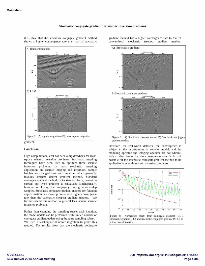
The results of the stochastic gradient and stochastic conjugate gradient method are given in Figure (3). The difference between the migrated image from SCG and that from SG are marginal, because in this much idealized testing, both methods can achieve good convergence. It is also clear that stochastic optimization results are quite comparable to that of conventional method using whole data space, which is given by Figure (2). The differences between these methods are prominent when we present the misfit as a function of iteration number in a log-scale view as shown in Figure (4). In general, the misfit drop from stochastic optimization is not as fast as that of regular using all the datasets, because of the stochastic nature of approximating the Hessian and the gradient. It is clear that stochastic optimizations demand more iterations to achieve the same level of misfit as that of regular inversion, which partially offset the saving of smaller size simulations required by each iteration. When we compare SCG and SG

Figure 1: Background reflectivity model


Main Menu

T


it is clear that the stochastic conjugate gradient method shows a higher convergence rate than that of stochastic

gradient. Conclusion High computational cost has been a big drawback for least-square seismic inversion problems. Stochastic sampling techniques have been used to optimize these seismic inversion problems. In most stochastic sampling application on seismic imaging and inversion, sample batches are changed over each iteration, which generally invokes steepest decent gradient method. Standard conjugate gradient method, in its standard form, cannot be carried out when gradient is calculated stochastically, because of losing the conjugacy during non-overlap samples. Stochastic conjugate gradient method for function approximation has shown promise with higher convergence rate than the stochastic steepest gradient method. We further extend this method to general least-square seismic inversion problems. Rather than changing the sampling subset each iteration, the model update can be performed with limited number of conjugate gradient update using the same sampling subset. We used a least-square Kirchoff migration to prove this method. The results show that the stochastic conjugate

gradient method has a higher convergence rate to that of conventional stochastic steepest gradient method.

However, for real-world datasets, the convergence is subject to the uncertainties in velocity model, and the modeling operator and imaging operator are not adjoint, which bring issues for the convergence rate. It is still possible for the stochastic conjugate gradient method to be applied to large scale seismic inversion problems.

A) Stochastic gradient

B) Stochastic conjugate gradient

Figure 3: A) Stochastic steepest decent B) Stochastic conjugate gradient method

A) Regular migration

B) LSM

Figure 2: (A) regular migration (B) Least square migration

Figure 4: Normalized misfit from conjugate gradient (CG), stochastic gradient (SG) and stochastic conjugate gradient (SCG) as a function of iteration.

006SEG Denver 2014 Annual MeetingDOI http://dx.doi.org/10.1190/segam2014-1442.1© 2014 SEG

Main Menu

T

http://dx.doi.org/10.1190/segam2014-1442.1 EDITED REFERENCES Note: This reference list is a copy-edited version of the reference list submitted by the author. Reference lists for the 2014 SEG Technical Program Expanded Abstracts have been copy edited so that references provided with the online metadata for each paper will achieve a high degree of linking to cited sources that appear on the Web. REFERENCES

Claerbout, J., 1985, Imaging the earth's interior: Blackwell Scientific Publishing.

Dai, W., X. Wang, and G. T. Schuster, 2011, Least-squares migration of multisource data with a deblurring filter: Geophysics, 76, no. 5, R135–R146, http://dx.doi.org/10.1190/geo2010-0159.1.

Huang, W., H. Ma, D. Vigh, J. Kapoor, K. Jiao, X. Cheng, and D. Sun, 2013, Velocity model building with long-offset and full-azimuth data: A case history for full-waveform inversion: 83rd Annual International Meeting, SEG, Expanded Abstracts, 4750–4754.

Jiang, H., and P. Wilford, 2012, A stochastic conjugate gradient method for approximation of functions : Journal of Computational and Applied Mathematics, 236, no. 9, 2529–2544, http://dx.doi.org/10.1016/j.cam.2011.12.012.

Krebs, J. R., J. E. Anderson, D. Hinkley, R. Neelamani, S. Lee, A. Baumstein, and M.-D. Lacasse, 2009, Fast full-wavefield seismic inversion using encoded sources: Geophysics, 74, no. 6, WCC177–WCC188, http://dx.doi.org/10.1190/1.3230502.

Leeuwen, T., A. Y. Aravkin, and F. Herrmann, 2011, Seismic waveform inversion by stochastic optimization: International Journal of Geophysics, 2011, doi: 10.1155/2011/689041.

Nemeth, T., C. Wu, and G. T. Schuster, 1999, Least-squares migration of incomplete reflection data: Geophysics, 64, 208–221, http://dx.doi.org/10.1190/1.1444517.

Schraudolph, N. N., and T. Graepel, 2003, Combining conjugate direction methods with stochastic approximation of gradients: 9th International Workshop on Artificial Intelligence and Statistics (AISTATS), Society for Artificial Intelligence and Statistic s, 7–13.

Tarantola , A., 1984, Inversion of seismic reflection data in the acoustic approximation: Geophysics, 49, 1259–1266.

Tarantola , A., 1986, A strategy for nonlinear elastic inversion of seismic reflection data: Geophysics, 51, 1893–1903, http://dx.doi.org/10.1190/1.1442046.

Vigh, D., and W. Starr, 2008, 3D prestack plane-wave, full-waveform inversion: Geophysics, 73, no. 5, VE135–VE144, http://dx.doi.org/10.1190/1.2952623.


Main Menu

T