Download - Spontaneous and Exponential Decay

INSTANCES: Incorporating Computational Scientific Thinking Advances into Education & Science Courses

1

Spontaneous and Exponential Decay

Learning goal: Students will understand some key aspects of spontaneous decay of radioactive nuclei and how to model them.

Learning objective

Science content objective:

• Students will understand how chance and randomness enter into some natural processes, and the conditions that lead to exponential decay (and growth).

Science model/computation objectives:

• Students will learn how to develop a simple model of the system that includes chance. • Students will understand the difference between mathematics that can predict a probability and

a computer simulation that predicts simulated, probablistic data. • Students will learn how to relate a probabilistic model and a computer simulation. • Students will understand that computer models can be used to explore and develop scientific

concepts by using a computer as a simulated laboratory.

Scientific skills objective:

• Students will practice the following scientific skills: o Graphing (visualizing) data. o Describing trends revealed by data. o Proportional reasoning and its limits. o Interpreting the contextual meaning of graphs. o Testing (confirm, modify or reject) hypothesis using simulated data.

Activities Overview

In this lesson, students will:

• Identify key objects or components within models and their relationships. • Make statements that describe characteristics of the system. • Make concept maps that incorporate components and relationships. • Create mathematical equations that describe the relationships that exist within the system. • Understand the use of iteration to relate solution at present time to that at future times. • Create or modify computer simulations of a model and analyze their predictions compared

to observed natural phenomena.


2

Products

At the end of this module students will produce and evaluate 1) a list of system statements, 2) concept maps, 3) mathematical equations and 4) a mathematical model implemented as computational simulation. Each product is a different view of the data and phenomenon.

Where’s Computational Scientific Thinking and Intuition Development

In this lesson students will construct a model and then a computer program that simulates the natural process of spontaneous, radioactive decay. A mathematical model can predict the probability of observing a specific number of particles, or the average number of particles observed, but it cannot

predict exactly what number will be observed for each measurement. In contrast, the computer program provides an actual simulation of the natural process, so that it is possible to observe the type of fluctuations that occur with natural data. In numerous ways the simulation is like doing an experiment on a computer.

After some discussion and experimentation, the students should come to realize that the computer simulation can be a more accurate description of nature than is the mathematical expression, the exponential function. A strong developmental understanding of the value of simulations is provided by hearing that the results of the simulation sound like an actual Geiger counter.

1. Observations and Problems Growth and decay occur frequently throughout the natural and manmade world. When the number of something increases with time, we have “growth”. When that number decreases with time we have “decay”. Depending on just how that number changes with time, we may have linear growth or decay, exponential growth or decay, or some other relation, such as periodic change.

The mathematical aspect of this module explores the properties of the equations that produce growth and decay, as well as the process of including chance into a mathematical and computational model.

Radioactive decay of nuclei is a natural process in which an unstable or excited nucleus emits energy in the form of a particle, with the nucleus usually changing from one chemical element to another. If the emitted particle can cause ionization (removal of electrons) of atoms, it can be detected with devices such as Geiger counters. The Geiger counter contains a tube filled with gas as well as separated metal plates or wires kept at a high voltage. When the charged particle passes through the gas, some of the gas atoms are ionized, and this leads to a current pulse through the plates. Each pulse is amplified,

An atom contains a cloud of electrons with a very tiny nucleus at its center. The nucleus contains neutrons and positively-‐charged protons. The negative charge of the electrons exactly matches the positive charge of the nucleus.

When the electrons in an atom get excited, they spontaneously deexcite and emit photons. Spontaneous decay also occurs within radioactive nuclei, with the nucleus emitting various particles. If the decay leads to a change in the number of protons in the nucleus, the atom changes from one chemical element to another.


3

counted and often converted to an audio beep. Each beep thus corresponds to an individual nuclear decay. Because the origin of the decay is a subatomic process governed by quantum mechanics, and because the rules of quantum mechanics are statistical in nature, there is always some randomness in the decay process, and this is usually heard as a noisy signal from the Geiger counter.

An example of a natural decay process is the radioactive conversion of a carbon-‐14 ( C !" ) nucleus into N

!" . Most carbon in our atmosphere is the stable isotope C !" , with some small fraction of it converted by cosmic rays to the radioactive isotope C !" . When a radioactive C !" nucleus decays, it emits an electron, and this converts the carbon nucleus into a N

!" nucleus (Figure 1). Here C !" would be called the “parent isotopes” and N

!" would be called the “daughter isotopes.” This radioactive decay is spontaneous with random fluctuations in the decay rate (the “stutter” heard with a Geiger counter).

Figure 1. is a schematic visualization of the radioactive decay of a single C !" nucleus into a N

!" nucleus plus a electron. The decay is spontaneous and random. “Spontaneous” means that a process

occurs on its own time scale without external stimulation. “Random” means that an element of chance is involved somewhere in the process, which means that it is impossible to know exactly when a single C !" nucleus decays. The only thing we know for sure is that the total number of C !" nuclei decreases in

time, while the total number of N !" increases in time accordingly.

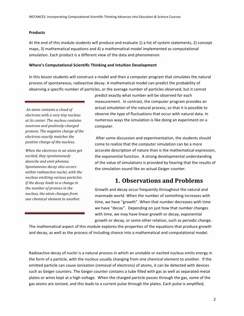
For example, we can measure how long it takes for one half of the C !" nuclei present in a sample to decay by measuring the decrease in activity (emission of electrons in a given period of time) of the sample. The time required for one half of a sample to decay is called the nucleus’s half-‐life 𝜏!/! (it is also the time for the activity to fall by a factor of 2). In general, after a time of 𝜏!/!, on the average, one half of the parent nuclei will decay into the daughter nuclei. In the next 𝜏!/!, half of the remaining nuclei will remain, which leaves ½ × ½ = ¼ of the original sample. In Figures 2 and 3 we show plots of the number of parent isotopes that have not yet decayed, as a function of time.

Figure 1 A schematic visualization of the radioactive (beta) decay of a single C !" nucleus into a N

!" nucleus plus a electron. The blue dots represent neutrons, the red dots protons. The decay is seen to transform a neutron into a proton. plus electron within the nucleus.

Figure 2 A histogram of experimental data showing the number of elementary particles (�! mesons) remaining as a function of time measured in nanoseconds (10!! s) [Stez] . The dashed curve is an exponential function fit to the data.


4

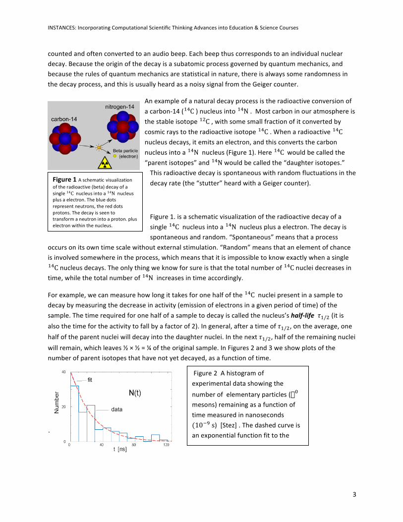
The rate of change in the number of decaying particles in Figures 2 and 3 are also examples of exponential decay. (In contrast, the increasing number of N

!" daughter nuclei created by the decay, the dashed line in Figure 3, is an example of growth, but not of exponential growth. The number of N

!" nuclei that are created exactly equals the number of C !" nuclei that decay.

A feature of radioactive decay is that each particle in the system has the same chance or probability to decay within a given time period. Because the exact moment when any one particle decays is random, it does not matter how long that particle has been around, or whether some nearby particle has already decayed. The probability of a nucleus decaying remains unchanged. Of course, once a C !" decays it becomes N

!" and will not be a C !" again.

The radioactive decay of C !" is used in so called radio-‐carbon dating, a method of estimating the age of once-‐living materials. Most of the carbon that plants absorb from the atmosphere is the stable isotope C!". Yet cosmic rays convert a known fraction of the C!" in the atmosphere to the radioactive (unstable) C !" isotope. So when plants absorb atmospheric carbon, they contain a known ratio of C !" 𝑡𝑜 C.

!" After the plant, or the animal that ate the plant, dies, the amount of C!" in it does not change (since it is stable), whereas the C !" in it decays to N.

!" Because the C !" in a dead object does not get replaced by the intake of fresh atmospheric carbon, the ratio of C !" to C !" in the artifact decreases over time, up until the point where there is no discernible C !" left (~10 half lives, about 60,000 year). By measuring the ratio of the amount of C !" to C !" , we can determine how much radiocarbon has decayed, and thereby date the artifact by making use of the known 5730 yrs half-‐life of C !" .

Problem 1) Determine how different assumptions about the rate of change of C !" lead to different time dependences of decay. 2) Once the mathematics of the first question is understood, develop a model for spontaneous decay that incorporates the inherent randomness of the process.

Background

Building a Concept Map of Model as Prelude to Equations

Concept maps graphically describe the system statements. We will place the components in boxes and show the relationships or processes as arrows. Here we use some simple concept maps to visualize several models and to assist in constructing the equations describing these models.

Figure 3


5

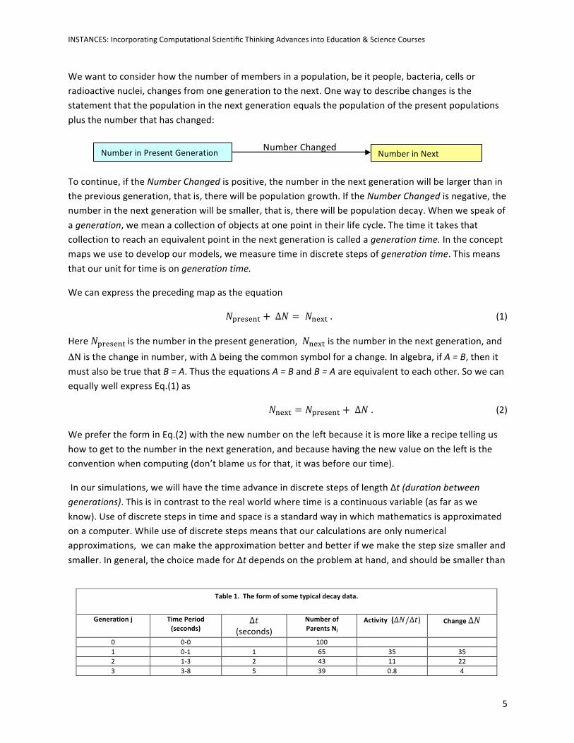
We want to consider how the number of members in a population, be it people, bacteria, cells or radioactive nuclei, changes from one generation to the next. One way to describe changes is the statement that the population in the next generation equals the population of the present populations plus the number that has changed:

To continue, if the Number Changed is positive, the number in the next generation will be larger than in the previous generation, that is, there will be population growth. If the Number Changed is negative, the number in the next generation will be smaller, that is, there will be population decay. When we speak of a generation, we mean a collection of objects at one point in their life cycle. The time it takes that collection to reach an equivalent point in the next generation is called a generation time. In the concept maps we use to develop our models, we measure time in discrete steps of generation time. This means that our unit for time is on generation time.

We can express the preceding map as the equation

𝑁!"#$#%& + ∆𝑁 = 𝑁!"#$ . (1)

Here 𝑁!"#$#%& is the number in the present generation, 𝑁!"#$ is the number in the next generation, and ΔN is the change in number, with Δ being the common symbol for a change. In algebra, if A = B, then it must also be true that B = A. Thus the equations A = B and B = A are equivalent to each other. So we can equally well express Eq.(1) as

𝑁!"#$ = 𝑁!"#$#%& + ∆𝑁 . (2)

We prefer the form in Eq.(2) with the new number on the left because it is more like a recipe telling us how to get to the number in the next generation, and because having the new value on the left is the convention when computing (don’t blame us for that, it was before our time).

In our simulations, we will have the time advance in discrete steps of length Δt (duration between generations). This is in contrast to the real world where time is a continuous variable (as far as we know). Use of discrete steps in time and space is a standard way in which mathematics is approximated on a computer. While use of discrete steps means that our calculations are only numerical approximations, we can make the approximation better and better if we make the step size smaller and smaller. In general, the choice made for Δt depends on the problem at hand, and should be smaller than

Table 1. The form of some typical decay data.

Generation j Time Period (seconds)

∆𝑡 (seconds)

Number of Parents Nj

Activity (∆𝑁/∆𝑡) Change ∆𝑁

0 0-‐0 100 1 0-‐1 1 65 35 35 2 1-‐3 2 43 11 22 3 3-‐8 5 39 0.8 4

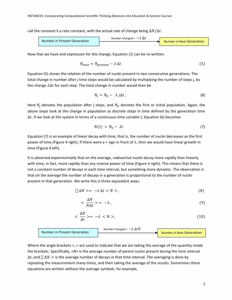
Number Changed Number in Next Number in Present Generation


6

the time it takes for any significant changes in the system.

For our decay model, we will use the generation time as the time step Δt. So the zeroth generation corresponds to the initial population at time t = 0. The first generation corresponds to the population at time t = ∆𝑡, the second generation corresponds to the population at time t = 2 ∆𝑡, and the jth generation to time 𝑡 = 𝑗 ∆𝑡. We can use the generation number as a subscript to denote generation; for example, N0 is the initial population number, N1 is the population of the first generation, N2 is the population of the second generation, and Nj is the population of the jth generation. For example, in Table 1 we see what some typical data might look like. (In reality, it is hard to measure the number of parents as a function of time, but straightforward to measure the number of decays ∆𝑁 and the activity ∆𝑁/∆𝑡.)

Mathematical Models

We want a model that will describe and predict the change in the population. As the simplest model of decay, let us assume that the decrease ∆𝑁 in the number of nuclei during each time interval ∆𝑡 is constant and call it 𝜆. In other words, the number of nuclei decreases always by 𝜆 from one generation to the next one. The mathematical expression of this statement is

∆𝑁 = −𝜆 ∆𝑡, (3)

Where the minus sign indicates a decrease, and the proportionality to ∆𝑡 means that the longer we wait, larger will be the number of decays. Equation (3) is often written in the form of a rate of change as

∆𝑁 ∆𝑡

= −𝜆, (4)

where rate means the change of something per unit time. Equation (4) says the change in number of nuclei over the change per unit time (rate) is equal to the loss of a constant number, 𝜆 . Accordingly, we

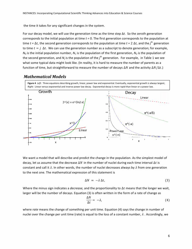
Figure 4 Left: Three equations describing growth, linear, power law and exponential. Eventually, exponential growth is always largest; Right: Linear versus exponential and inverse power law decay. Exponential decay is more rapid than linear or a power law.


7

call the constant λ a rate constant, with the actual rate of change being ∆𝑁/∆𝑡.

Now that we have and expression for the change, Equation (1) can be re-‐written:

𝑁!"#$ = 𝑁!"#$#%& − 𝜆 ∆𝑡 (5)

Equation (5) shows the relation of the number of nuclei present in two consecutive generations. The total change in number after j time steps would be calculated by multiplying the number of steps j, by the change 𝜆∆𝑡 for each step. The total change in number would then be

𝑁! = 𝑁! − 𝜆 𝑗∆𝑡 . (6)

Here 𝑁! denotes the population after j steps, and 𝑁! denotes the first or initial population. Again, the above steps look at the change in population as discrete steps in time defined by the generation time ∆𝑡. If we look at the system in terms of a continuous time variable t, Equation (6) becomes

𝑁(𝑡) = 𝑁! − 𝜆𝑡 (7)

Equation (7) is an example of linear decay with time, that is, the number of nuclei decreases as the first power of time (Figure 4 right). If there were a + sign in front of 𝜆, then we would have linear growth in time (Figure 4 left).

It is observed experimentally that on the average, radioactive nuclei decay more rapidly than linearly with time, in fact, more rapidly than any inverse power of time (Figure 4 right). This means that there is not a constant number of decays in each time interval, but something more dynamic. The observation is that on the average the number of decays in a generation is proportional to the number of nuclei present in that generation. We write this is three equivalent ways:

� ∆𝑁 >= −𝜆 ∆𝑡 < 𝑁 > , (8)

< ∆𝑁𝑁∆𝑡

> = −𝜆 , (9)

< ∆𝑁∆𝑡

>= −𝜆 < 𝑁 > , (10)

Where the angle brackets <..> are used to indicate that we are taking the average of the quantity inside the brackets. Specifically, <N> is the average number of parent nuclei present during the time interval ∆𝑡, and � ∆𝑁 > is the average number of decays in that time interval. The averaging is done by repeating the measurement many times, and then taking the average of the results. Sometimes these equations are written without the average symbols, for example,

Number Changed = −𝜆 ∆𝑡 Number in Next Generation Number in Present Generation

Number Changed = −𝜆 ∆𝑡𝑁 Number in Next Generation Number in Present Generation


8

∆𝑁 = −𝜆 ∆𝑡 𝑁. (11)

It is then to be understood that this is a probabilistic statement, that is, that the most likely decrease for ∆𝑁 is 𝜆 ∆𝑡 𝑁, but that a range of values is possible. On the average, however, the equation should hold true, at least within the expected statistical fluctuation. In all these equations we still call 𝜆 the decay rate constant, but as it appears in Equation (11) , it is now the probability of decay per unit time, per atom. So larger values of 𝜆 are now associated with more rapid (more radioactive) decay, with 𝜆 = 0 corresponding to no decay (a stable nucleus).

Nuclear and atomic decays are often called exponential decays based on the experimental data such as those shown in Figures 2 and 3-‐left. However, the mathematical exponential function describes the data only on the average, that is, the result obtained by repeating the experiment many times and averaging all of the results to reduce statistical fluctuations. Soon we will discuss the exponential function as it is used to describe decay. We actually will base our simulation directly on Equation (8) and not the exponential function.

Radioactivity

Often, experiments dealing with radioactivity do not measure the number of nuclei remaining as a function of time, but instead measure the number of decay per unit time ∆𝑁 ∆𝑡, also called the activity or decay rate. (Decay rates are easier to measure since the radioactive decay products can often be counted electronically in devices such as Geiger counters, whereas measuring the number of parent nuclei might require a chemical analysis of a sample for each time interval.) As we see from Equation (10), if N(t) decays exponentially, then the activity ∆𝑁 ∆𝑡, being proportional to N(t), will also decay exponentially with the same rate. In fact, it is the activity plotted in Figure 2.

Mathematics of the Exponential Function (Optional)

Equation (11) is our mathematical and computational model for exponential decay. Real experiments measure finite time internals ∆𝑡 and finite numbers ∆𝑁. If we idealize a real experiment to one that can measure infinitesimal times dt, and infinitesimal changes dN, then equation (8) becomes an equation involving the derivative

𝑑𝑁 𝑡𝑑𝑡

= −𝜆 𝑁 𝑡 , (11)

where N has now become a continuous function of the time variable t. If we next divide both sides of this equation by N(t), we obtain the equivalent form

𝑑𝑁 𝑡𝑁 𝑡

= −𝜆 𝑑𝑡. (12)

Equation (11) or (12) can be solved analytically using the techniques of differential calculus. In physics and engineering one tends to guess a solution of the form,

𝑁 𝑡 = 𝑁 0 𝑒!!" , (13)


9

and then verify that it works by substituting it into Eq.(12). In this way we know that (13) is a solution of (12) if N(0) is the number of nuclei at time t=0.

(**Mathematical Proof) A more systematic approach to the solution of (12) is to integrate it directly:

!" !! !

!! = −𝜆 𝑑𝑡!

! (14)

→ ln ! !! !

= −𝜆 𝑡 , (15)

where ln is the natural logarithm. Yet because ln 𝑒!! ! = −𝜆 𝑡, we can write (15) as

ln ! !! !

= ln 𝑒!! ! (16)

→ 𝑁 𝑡𝑁 0

= 𝑒!! ! , (17)

𝑁 𝑡 = 𝑁 0 𝑒!! ! . 𝐸𝑛𝑑 𝑜𝑓 𝑃𝑟𝑜𝑜𝑓 (18)

In these equations, e is a constant, 𝑒 ≅ 2.71828… , and is the base of the natural logarithms. And because any number raised to the zeroth power equals 1, Equation (18) does yield N(t) = N(0) at time t=0. The function 𝑒!! ! is an example of the exponential function, and this is the reason radioactive decay is also called exponential decay. The essential point in obtaining exponential decay or growth is that the rate of change of some quantity is proportional to the amount of that quantity present, precisely what is stated by equation (11).

Equations (13) contain the decay rate constant 𝜆 in the exponent. Another way to write these equations is in terms of a lifetime constant of the decaying nucleus

𝜏 = 1/𝜆 , (19)

𝑁 𝑡 = 𝑁 0 𝑒! !/! . (20)

Whereas Equation (20) using e is preferred in physics, in common usage the equation is often written in terms of powers of 2 rather than of e, and in terms of the half life 𝜏!/! instead of lifetime 𝜏:

𝑁 𝑡 = 𝑁 0 2𝑒! !/!!/! . (21)

As you can see in Figure 2, Equation (21) implies that after a time of one half-‐life 𝑖. 𝑒, 𝑡 = 𝜏!/!, the number of nuclei remaining is half of the original number:

𝑁 𝑡 = 𝜏!/! = 𝑁 0 2!! =𝑁 02

(22)

Likewise, after two half-‐lives, i.e., t = 2𝜏!/!, the number of nuclei has decayed by another factor of 2:


10

𝑁 𝑡 = 2𝜏!/! = 𝑁 𝑡 = 𝜏!/! 2!! = 𝑁 0 2!! =𝑁 04

(23)

For C !" , the half-‐life 𝜏!/! = 5730 years.

The three constants we have used to describe exponential decay are all related to each other by the natural logarithm of 2:

𝜏!/! = !" ! ! = 𝜏 ln 2. (24)

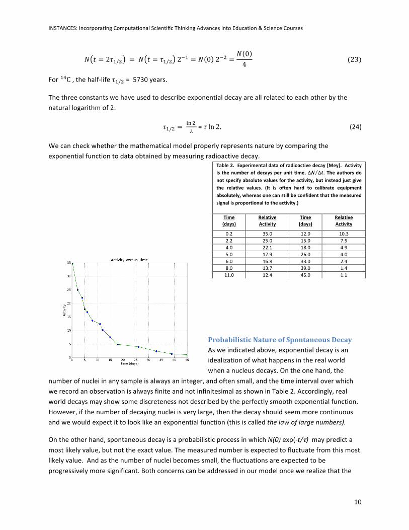
We can check whether the mathematical model properly represents nature by comparing the exponential function to data obtained by measuring radioactive decay.

Probabilistic Nature of Spontaneous Decay As we indicated above, exponential decay is an idealization of what happens in the real world when a nucleus decays. On the one hand, the

number of nuclei in any sample is always an integer, and often small, and the time interval over which we record an observation is always finite and not infinitesimal as shown in Table 2. Accordingly, real world decays may show some discreteness not described by the perfectly smooth exponential function. However, if the number of decaying nuclei is very large, then the decay should seem more continuous and we would expect it to look like an exponential function (this is called the law of large numbers).

On the other hand, spontaneous decay is a probabilistic process in which N(0) exp(-‐t/τ) may predict a most likely value, but not the exact value. The measured number is expected to fluctuate from this most likely value. And as the number of nuclei becomes small, the fluctuations are expected to be progressively more significant. Both concerns can be addressed in our model once we realize that the

Table 2. Experimental data of radioactive decay [Mey]. Activity is the number of decays per unit time, ∆𝑵 ∆𝒕. The authors do not specify absolute values for the activity, but instead just give the relative values. (It is often hard to calibrate equipment absolutely, whereas one can still be confident that the measured signal is proportional to the activity.)

Time (days)

Relative Activity

Time (days)

Relative Activity

0.2 35.0 12.0 10.3 2.2 25.0 15.0 7.5 4.0 22.1 18.0 4.9 5.0 17.9 26.0 4.0 6.0 16.8 33.0 2.4 8.0 13.7 39.0 1.4 11.0 12.4 45.0 1.1


11

mathematical description yields a most probable value of the number of nuclei that have decays, and that likely value should be close to the one obtained on the average. This means that if experimental observations of spontaneous decay starting with the same number of nuclei are repeated many times, then the average of the experimental results should be described by an exponential function.

Computer Simulation of Equation (5)

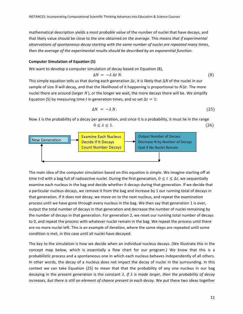
We want to develop a computer simulation of decay based on Equation (8), ∆𝑁 = −𝜆 ∆𝑡 𝑁. (8)

This simple equation tells us that during each generation ∆𝑡, it is likely that ∆𝑁 of the nuclei in our sample of size 𝑁 will decay, and that the likelihood of it happening is proportional to 𝑁∆𝑡. The more nuclei there are around (larger 𝑁 ), or the longer we wait, the more decays there will be. We simplify Equation (5) by measuring time t in generation times, and so set ∆𝑡 = 1:

∆𝑁 = −𝜆 𝑁 . (25)

Now 𝜆 is the probability of a decay per generation, and since it is a probability, it must lie in the range 0 ≤ 𝜆 ≤ 1. (26)

The main idea of the computer simulation based on this equation is simple. We imagine starting off at time t=0 with a bag full of radioactive nuclei. During the first generation, 0 ≤ 𝑡 ≤ ∆𝑡, we sequentially examine each nucleus in the bag and decide whether it decays during that generation. If we decide that a particular nucleus decays, we remove it from the bag and increase by 1 our running total of decays in that generation. If it does not decay, we move on to the next nucleus, and repeat the examination process until we have gone through every nucleus in the bag. We then say that generation 1 is over, output the total number of decays in that generation and decrease the number of nuclei remaining by the number of decays in that generation. For generation 2, we reset our running total number of decays to 0, and repeat the process with whatever nuclei remain in the bag. We repeat the process until there are no more nuclei left. This is an example of iteration, where the same steps are repeated until some condition is met, in this case until all nuclei have decayed.

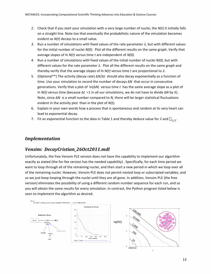
The key to the simulation is how we decide when an individual nucleus decays. (We illustrate this in the concept map below, which is essentially a flow chart for our program.) We know that this is a probabilistic process and a spontaneous one in which each nucleus behaves independently of all others. In other words, the decay of a nucleus does not impact the decay of nuclei in the surrounding. In this context we can take Equation (25) to mean that that the probability of any one nucleus in our bag decaying in the present generation is the constant 𝜆. If 𝜆 is made larger, then the probability of decay increases, but there is still an element of chance present in each decay. We put these two ideas together

New Generation Examine Each Nucleus Decide If It Decays Count Number Decays

Output Number of Decays Decrease N by Number of Decays Quit if No Nuclei Remain


12

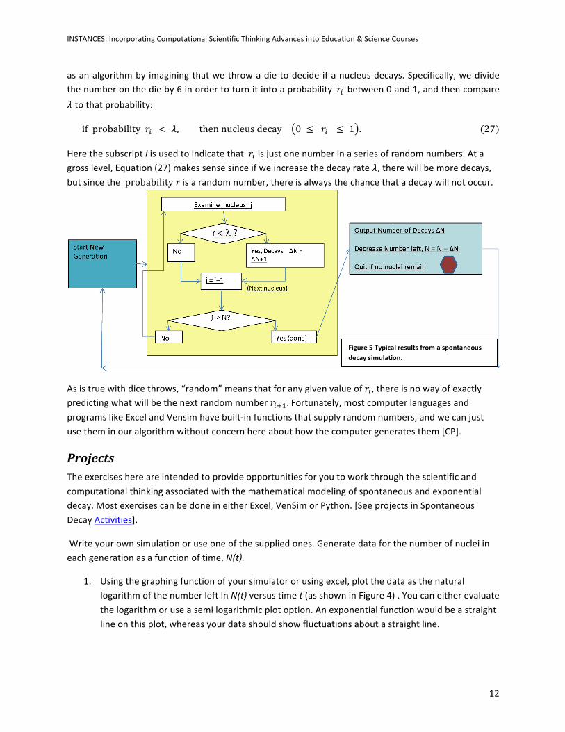
as an algorithm by imagining that we throw a die to decide if a nucleus decays. Specifically, we divide the number on the die by 6 in order to turn it into a probability 𝑟! between 0 and 1, and then compare 𝜆 to that probability:

if probability 𝑟! < 𝜆, then nucleus decay 0 ≤ 𝑟! ≤ 1 . (27)

Here the subscript i is used to indicate that 𝑟! is just one number in a series of random numbers. At a gross level, Equation (27) makes sense since if we increase the decay rate 𝜆, there will be more decays, but since the probability 𝑟 is a random number, there is always the chance that a decay will not occur.

As is true with dice throws, “random” means that for any given value of 𝑟!, there is no way of exactly predicting what will be the next random number 𝑟!!!. Fortunately, most computer languages and programs like Excel and Vensim have built-‐in functions that supply random numbers, and we can just use them in our algorithm without concern here about how the computer generates them [CP].

Projects The exercises here are intended to provide opportunities for you to work through the scientific and computational thinking associated with the mathematical modeling of spontaneous and exponential decay. Most exercises can be done in either Excel, VenSim or Python. [See projects in Spontaneous Decay Activities].

Write your own simulation or use one of the supplied ones. Generate data for the number of nuclei in each generation as a function of time, N(t).

1. Using the graphing function of your simulator or using excel, plot the data as the natural logarithm of the number left ln N(t) versus time t (as shown in Figure 4) . You can either evaluate the logarithm or use a semi logarithmic plot option. An exponential function would be a straight line on this plot, whereas your data should show fluctuations about a straight line.

Figure 5 Typical results from a spontaneous decay simulation.


13

04008001200t

0

2

4

100,00010,0001,000100

10

log[N(t)]

2. Check that if you start your simulation with a very large number of nuclei, the N(t) it initially falls on a straight line. Note too that eventually the probabilistic nature of the simulation becomes evident as N(t) decays to a small value.

3. Run a number of simulations with fixed values of the rate parameter 𝜆, but with different values for the initial number of nuclei N(0). Plot all the different results on the same graph. Verify that average slopes of ln N(t) versus time t are independent of N(0).

4. Run a number of simulations with fixed values of the initial number of nuclei N(0), but with different values for the rate parameter 𝜆. Plot all the different results on the same graph and thereby verify that the average slopes of ln N(t) versus time t are proportional to 𝜆.

5. (Optional**) The activity (decay rate) ΔN/Δt should also decay exponentially as a function of time. Use your simulation to record the number of decays ΔN that occur in consecutive generations. Verify that a plot of ln(ΔN) versus time t has the same average slope as a plot of ln N(t) versus time (because Δt =1 in all our simulations, we do not have to divide ΔN by it) . Note, since ΔN is a small number compared to N, there will be larger statistical fluctuations evident in the activity plot than in the plot of N(t).

6. Explain in your own words how a process that is spontaneous and random at its very heart can lead to exponential decay.

7. Fit an exponential function to the data in Table 1 and thereby deduce value for 𝜆 and �!/!.

Implementation

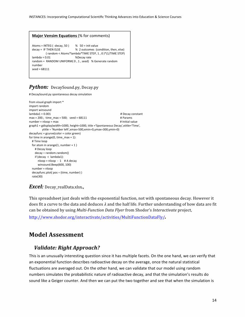
Vensim: DecayCristian_26Oct2011.mdl Unfortunately, the free Vensim PLE version does not have the capability to implement our algorithm exactly as stated (the for-‐fee version has the needed capability) . Specifically, for each time period we want to loop through all of the remaining nuclei, and then start a new period in which we loop over all of the remaining nuclei. However, Vensim PLE does not permit nested loop or subscripted variables, and so we just keep looping through the nuclei until they are all gone. In addition, Vensim PLE (the free version) eliminates the possibility of using a different random number sequence for each run, and so you will obtain the same results for every simulation. In contrast, the Python program listed below is seen to implement the algorithm as desired.


14

Python: DecaySound.py, Decay.py # DecaySound.py spontaneous decay simulation from visual.graph import * import random import winsound lambda1 = 0.001 # Decay constant max = 200.; time_max = 500; seed = 68111 # Params number = nloop = max # Initial value graph1 = gdisplay(width=1000, height=1000, title ='Spontaneous Decay',xtitle='Time', ytitle = 'Number left',xmax=500,xmin=0,ymax=300,ymin=0) decayfunc = gcurve(color = color.green) for time in arange(0, time_max + 1): # Time loop for atom in arange(1, number + 1 ) # Decay loop decay = random.random() if (decay < lambda1): nloop = nloop -‐ 1 # A decay winsound.Beep(600, 100) number = nloop decayfunc.plot( pos = (time, number) ) rate(30)

Excel: Decay_realData.xlsx.,

This spreadsheet just deals with the exponential function, not with spontaneous decay. However it does fit a curve to the data and deduces 𝜆 and the half life. Further understanding of how data are fit can be obtained by using Multi-‐Function Data Flyer from Shodor’s Interactivate project, http://www.shodor.org/interactivate/activities/MultiFunctionDataFly/.

Model Assessment

Validate: Right Approach? This is an unusually interesting question since it has multiple facets. On the one hand, we can verify that an exponential function describes radioactive decay on the average, once the natural statistical fluctuations are averaged out. On the other hand, we can validate that our model using random numbers simulates the probabilistic nature of radioactive decay, and that the simulation’s results do sound like a Geiger counter. And then we can put the two together and see that when the simulation is

Major Vensim Equations (% for comments) Atoms = INTEG ( -‐decay, 50 ) % 50 = init value decay = IF THEN ELSE % 2 outcomes (condition, then, else) ( random < Atoms*lambda*TIME STEP, 1 , 0 )*(1/TIME STEP) lambda = 0.01 %Decay rate random = RANDOM UNIFORM( 0 , 1 , seed) % Generate random number seed = 68111


15

run for very large numbers of particles, which tends to minimize the statistical fluctuations, we obtain results that look like exponential decay (a straight line on a semi log plot).

On a more fundamental level, one can ask how do you really know that the experimental results are spontaneous and contain randomness. Not a simple question to answer, in part because the role of randomness in science is a fundamental question. One answer is that radioactive decay is often the definition used to define a naturally random process. Another answer is that our simulation using random numbers sounds and looks like the natural process, which implies that the natural process probably has randomness too.

Verify: Mistakes? The biggest point here might be to question whether the computer’s random number generator (which really cannot be random since it uses a deterministic algorithm), does in fact produce a good approximation to random numbers. We can talk about that, as in [CP], but it tends to get rather mathematical.

The agreement of the simulation’s results with large numbers and the analytic exponential function is also a good verification.

The fact that the slope of lnN(t) versus t remains the same for different values of the initial population is good test of the simulation, since that is true in nature as well.

The variation of the slope as we change the value of the decay parameter 𝜆 is a good test of the model and the simulation.

The verification that both N(t) and ΔN(t)/ Δt have the same slope is both a validation of the theory being a good description of nature and a verification of our computation.

Where's the Math? An understanding of the exponential function, with its relation to half lives and rate constants, is an important mathematical description of natural phenomena. Likewise, the derivation of the exponential function from our discrete equations is pure calculus, as is the integration of the differential equation and the expression of its answer in various forms. The comparison of linear growth and exponential growth, and the different assumptions that lead to each, is pure math.

Exact, Approximate, Precision, Accuracy, Uncertainties All of these considerations enter into this project, sometimes in rather subtle ways. Our discrete math equation ∆𝑁 = −𝜆 ∆𝑡 𝑁, is really the most `exact’ description we have, since the process is probabilistic. The exponential function is analytic, but only approximates nature on the average. (This is an interesting reversal of the usual situation.) There are uncertainties in the project due to its statistical nature, but this is as it should be since it is true in nature as well. We have not tested the precision of our random number generator, as would a researcher, but it is a concern that is good to keep in mind.


16

Summary and Conclusions

Where's Computational Scientific Thinking We are given a natural phenomenon that most textbooks treat only in an approximate way (although they often do not indicate that) by saying an exponential function described radioactive decay. This is only true on the average since the real phenomenon is a probabilistic process. This is a good example of the use a computer and its random number generator to simulate the natural process. We also recognize that the natural process is a discrete process in terms of time intervals and number of counts, which again we simulate with our computer model. The simulation truly provides a numerical laboratory in which to experiment. This is precisely how simulation adds to theory and experiments as pillars of science.

The simulation itself employs a recursion relation to take one generation to the next, and keeps repeating the same rule until no nuclei are left. This is in contrast to just solving for the final answer.

References [Mey] S. Meyer and E. von Schweidler, Sitzungberichte der Akademie der Wissenschaften zu Wien, Mathematisch-‐Naturwissenschaftliche Classe, p. 1202 (Table 5), 1905, as reported in J. Tukey, Exploratory Data Analysis, Addison-‐Wesley, 1977.

[CP] Landau, R.H., M.J. Paez and C.C. Bordeianu, (2008), A Survey of Computational Physics, Chapter 5, Princeton Univ. Press, Princeton.

[Stez] STETZ, A., J. CARROLL, N. CHIRAPATPIMOL, M. DIXIT, G. IGO, M. NASSER, D. ORTENDAHL, AND V. PEREZ-‐MENDEZ (1973), “Determination of the Axial Vector Form Factor in the Radiative Decay of the Pion”, LBL 1707, invited paper at the Symposium of the Division of Nuclear Physics, Washington, DC, April. 221