

![Mathematical Models in Biology - Bio · PDF fileMathematical Models in Biology ... J.D., Mathematical Biology, Springer, 1989, [19] Edelstein-Keshet, Leah, Mathematical models in biology,](https://static.fdocuments.net/doc/165x107/5ab3fe3b7f8b9a7c5b8b587a/mathematical-models-in-biology-bio-models-in-biology-jd-mathematical-biology.jpg)


Languages
Pages
Legal

Some mathematicalmodels of evolution
III: The infinitesimal model
Alison EtheridgeUniversity of Oxford

Thanks
Nick Barton Amandine Veber
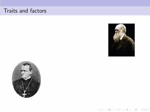
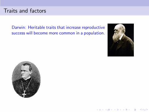
Traits and factors
Traits and factors
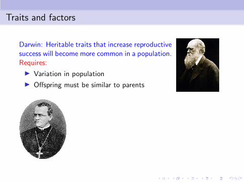
Darwin: Heritable traits that increase reproductivesuccess will become more common in a population.
Traits and factors
Darwin: Heritable traits that increase reproductivesuccess will become more common in a population.Requires:
◮ Variation in population
◮ Offspring must be similar to parents
Traits and factors
Darwin: Heritable traits that increase reproductivesuccess will become more common in a population.Requires:
◮ Variation in population
◮ Offspring must be similar to parents
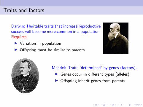
Mendel: Traits ‘determined’ by genes (factors).
◮ Genes occur in different types (alleles)
◮ Offspring inherit genes from parents
Complex traits?
Complex traits?
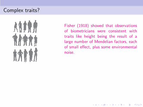
Fisher (1918) showed that observationsof biometricians were consistent withtraits like height being the result of alarge number of Mendelian factors, eachof small effect, plus some environmentalnoise.

Complex traits?
Fisher (1918) showed that observationsof biometricians were consistent withtraits like height being the result of alarge number of Mendelian factors, eachof small effect, plus some environmentalnoise.
Toy example: M genes, each with 2 alleles, effects ±1/√M on
trait, say. Genetic component trait value
Z = z0 +
M∑
l=1
ηl√M,
where ηl = ±1 with equal probability.
Fisher and natural selection
Fisher’s infinitesimal model: the (genetic component of the) traitvalue of the offspring of two unrelated parents is the mean of theparental trait values plus a normally distributed error with meanzero and variance the additive genetic variance.
Fisher and natural selection
Fisher’s infinitesimal model: the (genetic component of the) traitvalue of the offspring of two unrelated parents is the mean of theparental trait values plus a normally distributed error with meanzero and variance the additive genetic variance.
Fisher’s fundamental theorem of natural selection: the rate ofincrease in mean fitness is proportional to the additive geneticvariance in fitness.
“Natural selection is a mechanism for generating an exceedinglyhigh degree of improbability.”
The basic model
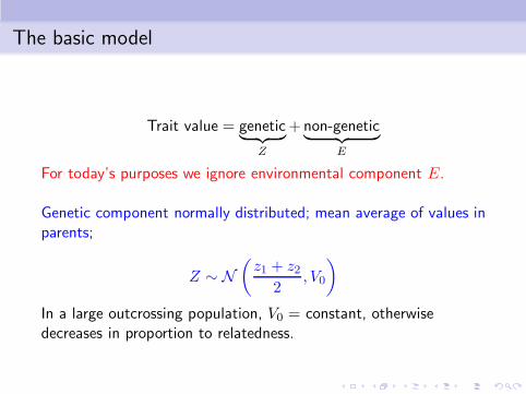
Trait value = genetic︸ ︷︷ ︸
Z
+ non-genetic︸ ︷︷ ︸
E
For today’s purposes we ignore environmental component E.
Genetic component normally distributed; mean average of values inparents;
Z ∼ N(z1 + z2
2, V0
)
In a large outcrossing population, V0 = constant, otherwisedecreases in proportion to relatedness.
The simplest case
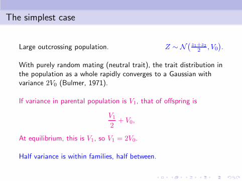
Large outcrossing population. Z ∼ N(z1+z2
2 , V0).
With purely random mating (neutral trait), the trait distribution inthe population as a whole rapidly converges to a Gaussian withvariance 2V0 (Bulmer, 1971).
If variance in parental population is V1, that of offspring is
V12
+ V0,
At equilibrium, this is V1, so V1 = 2V0.
Half variance is within families, half between.
IN GENERAL THE INFINITESIMAL MODEL ONLY SAYS THATTHE GENETIC COMPONENTS WITHIN FAMILIES ARENORMALLY DISTRIBUTED. THE DISTRIBUTION ACROSSTHE WHOLE POPULATION MAY BE FAR FROM NORMAL.
IN GENERAL THE INFINITESIMAL MODEL ONLY SAYS THATTHE GENETIC COMPONENTS WITHIN FAMILIES ARENORMALLY DISTRIBUTED. THE DISTRIBUTION ACROSSTHE WHOLE POPULATION MAY BE FAR FROM NORMAL.
Trait distributions within families are normally distributed, with avariance-covariance matrix that is determined entirely by that in anancestral population and the probabilities of identity determined bythe pedigree.
As a result of the multivariate normality, conditioning on sometrait values within the pedigree has predictable effects on the meanand variance within and between families.
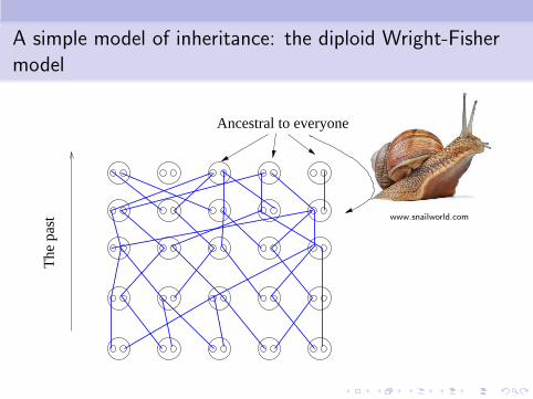
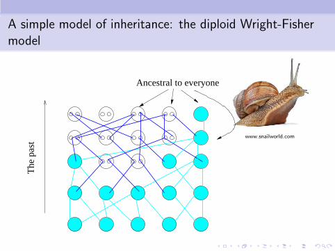
A simple model of inheritance: the diploid Wright-Fishermodel
www.snailworld.com
Ancestral to everyone
The
pas
t
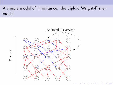
A simple model of inheritance: the diploid Wright-Fishermodel
www.snailworld.com
The
pas
t
Ancestral to everyone
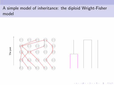
A simple model of inheritance: the diploid Wright-Fishermodel
Ancestral to everyone
The
pas
t
A simple model of inheritance: the diploid Wright-Fishermodel
The
pas
t
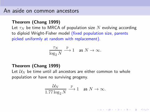
An aside on common ancestors
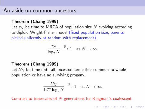
Theorem (Chang 1999)Let τN be time to MRCA of population size N evolving accordingto diploid Wright-Fisher model (fixed population size, parentspicked uniformly at random with replacement).
τNlog2N
P−→ 1 as N → ∞.
Theorem (Chang 1999)Let UN be time until all ancestors are either common to wholepopulation or have no surviving progeny.
UN
1.77 log2N
P−→ 1 as N → ∞.
An aside on common ancestors
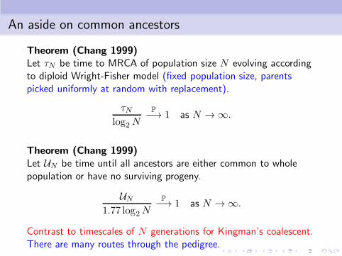
Theorem (Chang 1999)Let τN be time to MRCA of population size N evolving accordingto diploid Wright-Fisher model (fixed population size, parentspicked uniformly at random with replacement).
τNlog2N
P−→ 1 as N → ∞.
Theorem (Chang 1999)Let UN be time until all ancestors are either common to wholepopulation or have no surviving progeny.
UN
1.77 log2N
P−→ 1 as N → ∞.
Contrast to timescales of N generations for Kingman’s coalescent.
An aside on common ancestors
Theorem (Chang 1999)Let τN be time to MRCA of population size N evolving accordingto diploid Wright-Fisher model (fixed population size, parentspicked uniformly at random with replacement).
τNlog2N
P−→ 1 as N → ∞.
Theorem (Chang 1999)Let UN be time until all ancestors are either common to wholepopulation or have no surviving progeny.
UN
1.77 log2N
P−→ 1 as N → ∞.
Contrast to timescales of N generations for Kingman’s coalescent.There are many routes through the pedigree.
Pedigrees and matrices
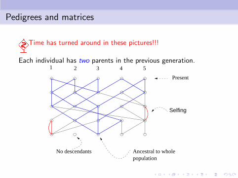
�Time has turned around in these pictures!!!
Each individual has two parents in the previous generation.
No descendants Ancestral to wholepopulation
Present
Selfing
21 3 4 5
Pedigrees and matrices
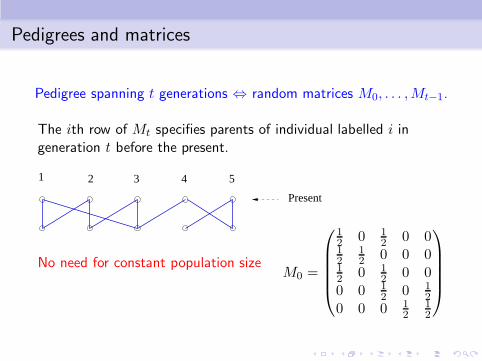
Pedigree spanning t generations ⇔ random matrices M0, . . . ,Mt−1.
The ith row of Mt specifies parents of individual labelled i ingeneration t before the present.
Present
21 3 4 5
No need for constant population sizeM0 =
12 0 1
2 0 012
12 0 0 0
12 0 1
2 0 00 0 1
2 0 12
0 0 0 12
12
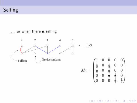
Selfing
. . . or when there is selfing
21 3 4 5
t=3
No descendantsSelfing
M3 =
1 0 0 0 012 0 1
2 0 012 0 1
2 0 00 0 1
212 0
0 0 0 12
12
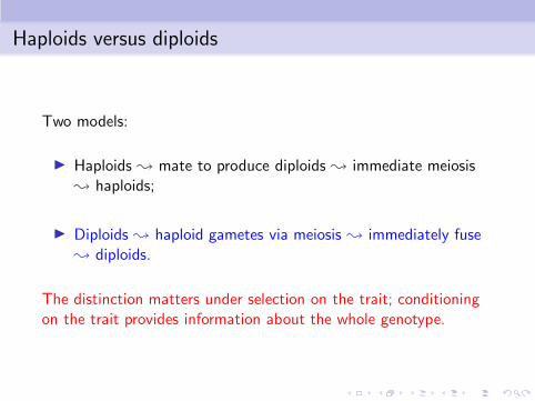
Haploids versus diploids
Two models:
◮ Haploids ❀ mate to produce diploids ❀ immediate meiosis❀ haploids;
◮ Diploids ❀ haploid gametes via meiosis ❀ immediately fuse❀ diploids.
The distinction matters under selection on the trait; conditioningon the trait provides information about the whole genotype.
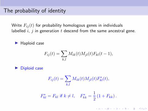
The probability of identity
Write Fij(t) for probability homologous genes in individualslabelled i, j in generation t descend from the same ancestral gene.
◮ Haploid case
Fij(t) =∑
k,l
Mik(t)Mjl(t)Fkl(t− 1),
◮ Diploid case
Fij(t) =∑
k,l
Mik(t)Mjl(t)F∗
kl(t),
F ∗
kl = Fkl if k 6= l, F ∗
kk =1
2(1 + Fkk) .
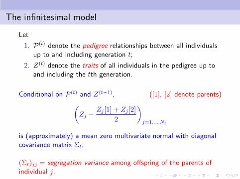
The infinitesimal model
Let
1. P(t) denote the pedigree relationships between all individualsup to and including generation t;
2. Z(t) denote the traits of all individuals in the pedigree up toand including the tth generation.
Conditional on P(t) and Z(t−1), ([1], [2] denote parents)
(
Zj −Zj [1] + Zj[2]
2
)
j=1,...,Nt
is (approximately) a mean zero multivariate normal with diagonalcovariance matrix Σt.
(Σt)jj = segregation variance among offspring of the parents ofindividual j.
Why might it be a reasonable model?
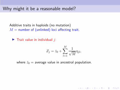
Additive traits in haploids (no mutation)M = number of (unlinked) loci affecting trait.
◮ Trait value in individual j:
Zj = z0 +
M∑
l=1
1√Mηjl,
where z0 = average value in ancestral population.
Why might it be a reasonable model?
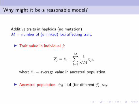
Additive traits in haploids (no mutation)M = number of (unlinked) loci affecting trait.
◮ Trait value in individual j:
Zj = z0 +
M∑
l=1
1√Mηjl,
where z0 = average value in ancestral population.
◮ Ancestral population. ηjl i.i.d (for different j), say.
Reproduction
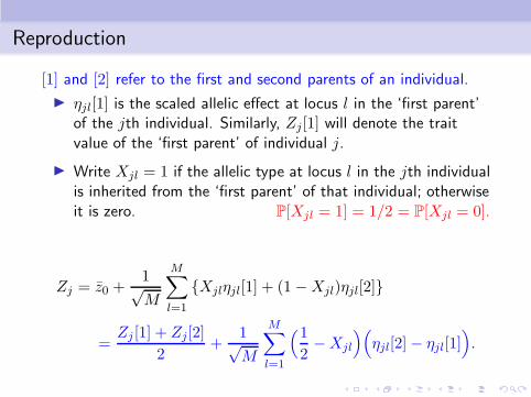
[1] and [2] refer to the first and second parents of an individual.
◮ ηjl[1] is the scaled allelic effect at locus l in the ‘first parent’of the jth individual. Similarly, Zj[1] will denote the traitvalue of the ‘first parent’ of individual j.
◮ Write Xjl = 1 if the allelic type at locus l in the jth individualis inherited from the ‘first parent’ of that individual; otherwiseit is zero. P[Xjl = 1] = 1/2 = P[Xjl = 0].
Zj = z0 +1√M
M∑
l=1
{Xjlηjl[1] + (1−Xjl)ηjl[2]}
=Zj [1] + Zj[2]
2+
1√M
M∑
l=1
(1
2−Xjl
)(
ηjl[2]− ηjl[1])
.
Conditioning
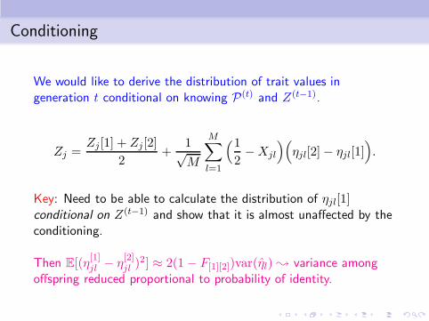
We would like to derive the distribution of trait values ingeneration t conditional on knowing P(t) and Z(t−1).
Zj =Zj [1] + Zj[2]
2+
1√M
M∑
l=1
(1
2−Xjl
)(
ηjl[2]− ηjl[1])
.
Key: Need to be able to calculate the distribution of ηjl[1]conditional on Z(t−1) and show that it is almost unaffected by theconditioning.
Then E[(η[1]jl − η
[2]jl )
2] ≈ 2(1 − F[1][2])var(ηl) ❀ variance amongoffspring reduced proportional to probability of identity.
Back to our toy example
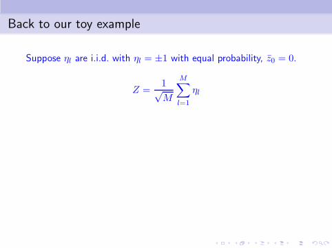
Suppose ηl are i.i.d. with ηl = ±1 with equal probability, z0 = 0.
Z =1√M
M∑
l=1
ηl
Back to our toy example
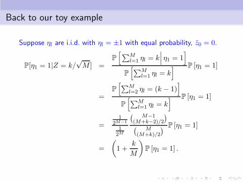
Suppose ηl are i.i.d. with ηl = ±1 with equal probability, z0 = 0.
P[η1 = 1|Z = k/√M ] =
P
[∑M
l=1 ηl = k∣∣∣ η1 = 1
]
P
[∑M
l=1 ηl = k] P [η1 = 1]
=P
[∑M
l=2 ηl = (k − 1)]
P
[∑M
l=1 ηl = k] P [η1 = 1]
=1
2M−1
12M
( M−1(M+k−2)/2
)
(M
(M+k)/2
) P [η1 = 1]
=
(
1 +k
M
)
P [η1 = 1] .
Toy example continued
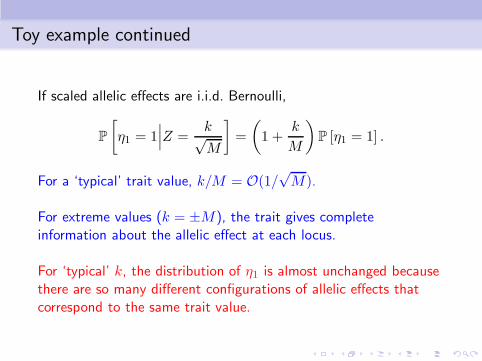
If scaled allelic effects are i.i.d. Bernoulli,
P
[
η1 = 1∣∣∣Z =
k√M
]
=
(
1 +k
M
)
P [η1 = 1] .
For a ‘typical’ trait value, k/M = O(1/√M).
For extreme values (k = ±M), the trait gives completeinformation about the allelic effect at each locus.
For ‘typical’ k, the distribution of η1 is almost unchanged becausethere are so many different configurations of allelic effects thatcorrespond to the same trait value.
The infinitesimal model
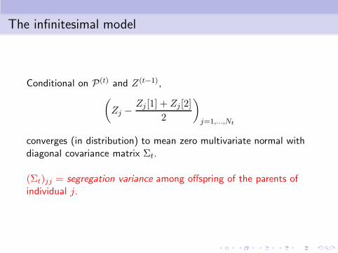
Conditional on P(t) and Z(t−1),
(
Zj −Zj [1] + Zj[2]
2
)
j=1,...,Nt
converges (in distribution) to mean zero multivariate normal withdiagonal covariance matrix Σt.
(Σt)jj = segregation variance among offspring of the parents ofindividual j.
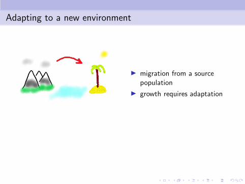
Adapting to a new environment
◮ migration from a sourcepopulation
◮ growth requires adaptation
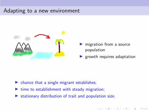
Adapting to a new environment
◮ migration from a sourcepopulation
◮ growth requires adaptation
◮ chance that a single migrant establishes;
◮ time to establishment with steady migration;
◮ stationary distribution of trait and population size.
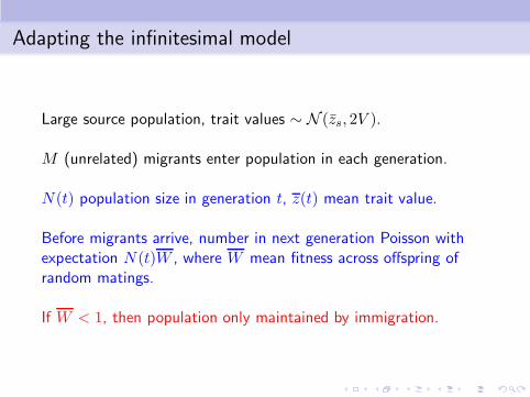
Adapting the infinitesimal model
Large source population, trait values ∼ N (zs, 2V ).
M (unrelated) migrants enter population in each generation.
N(t) population size in generation t, z(t) mean trait value.
Before migrants arrive, number in next generation Poisson withexpectation N(t)W , where W mean fitness across offspring ofrandom matings.
If W < 1, then population only maintained by immigration.
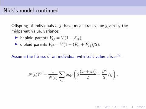
Nick’s model continued
Offspring of individuals i, j, have mean trait value given by themidparent value, variance:
◮ haploid parents Vij = V (1− Fij),
◮ diploid parents Vij = V (1− (Fii + Fjj)/2).
Assume the fitness of an individual with trait value z is eβz.
N(t)W =1
N(t)
∑
i,j
exp
(
β(zi + zj)
2+β2
2Vij
)
.
Expect density dependent fitness and stabilising selection toultimately limit population size; assuming established before theseare significant.
A single migrant, trait value z0 (diploid)
-� -� �����
-�
��-�
�����
����
���
�
�
-� -� -� -� � �����
-�
��-�
�����
����
���
�
�
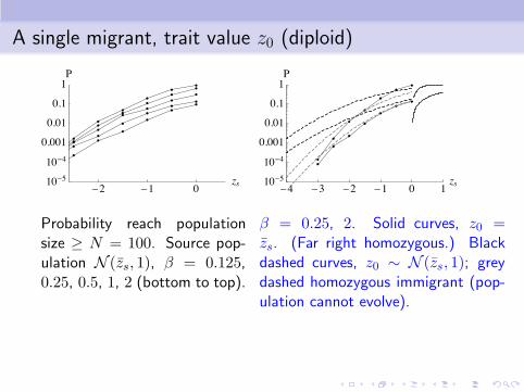
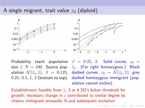
Probability reach populationsize ≥ N = 100. Source pop-ulation N (zs, 1), β = 0.125,0.25, 0.5, 1, 2 (bottom to top).
β = 0.25, 2. Solid curves, z0 =zs. (Far right homozygous.) Blackdashed curves, z0 ∼ N (zs, 1); greydashed homozygous immigrant (pop-ulation cannot evolve).
A single migrant, trait value z0 (diploid)
-� -� �����
-�
��-�
�����
����
���
�
�
-� -� -� -� � �����
-�
��-�
�����
����
���
�
�
Probability reach populationsize ≥ N = 100. Source pop-ulation N (zs, 1), β = 0.125,0.25, 0.5, 1, 2 (bottom to top).
β = 0.25, 2. Solid curves, z0 =zs. (Far right homozygous.) Blackdashed curves, z0 ∼ N (zs, 1); greydashed homozygous immigrant (pop-ulation cannot evolve).
Establishment feasible from zs 3 or 4 SD’s below threshold forgrowth; necessary change in z contributed to similar degree bychance immigrant unusually fit,and subsequent evolution
Successful establishment
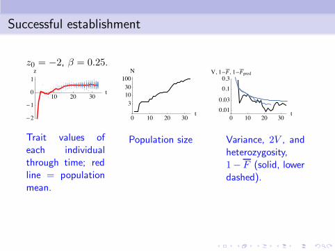
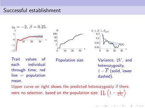
z0 = −2, β = 0.25.
�� �� ���
-�
-�
�
�
�
� �� �� ���
�
��
��
���
�
� �� �� ���
����
����
���
���
�-� �-�����
Trait values ofeach individualthrough time; redline = populationmean.
Population size Variance, 2V , andheterozygosity,1− F (solid, lowerdashed).
Successful establishment
z0 = −2, β = 0.25.
�� �� ���
-�
-�
�
�
�
� �� �� ���
�
��
��
���
�
� �� �� ���
����
����
���
���
�-� �-�����
Trait values ofeach individualthrough time; redline = populationmean.
Population size Variance, 2V , andheterozygosity,1− F (solid, lowerdashed).
Upper curve on right shows the predicted heterozygosity if there
were no selection, based on the population size:∏
t
(
1− 12Nt
)
.
Steady migration: a ‘deterministic’ model
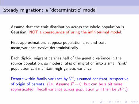
Assume that the trait distribution across the whole population isGaussian. NOT a consequence of using the infinitesimal model.
First approximation: suppose population size and traitmean/variance evolve deterministically.
Each diploid migrant carrries half of the genetic variance in thesource population, so modest rates of migration into a small ‘sink’population can maintain high genetic variance.
Denote within family variance by V ∗, assumed constant irrespectiveof origin of parents. (i.e. Assume F = 0, but can be a bit moresophisticated. Recall variance across population will then be 2V ∗.)
A recursion
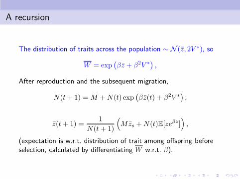
The distribution of traits across the population ∼ N (z, 2V ∗), so
W = exp(βz + β2V ∗
),
After reproduction and the subsequent migration,
N(t+ 1) =M +N(t) exp(βz(t) + β2V ∗
);
z(t+ 1) =1
N(t+ 1)
(
Mzs +N(t)E[zeβz ])
,
(expectation is w.r.t. distribution of trait among offspring beforeselection, calculated by differentiating W w.r.t. β).
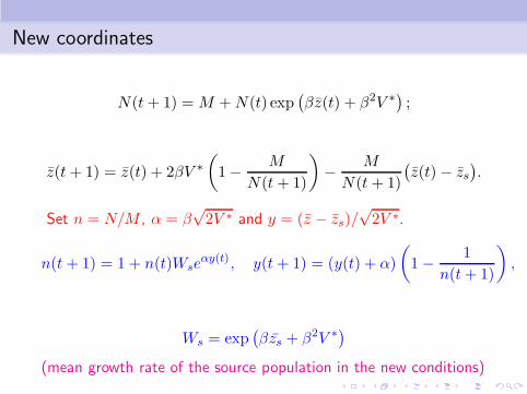
New coordinates
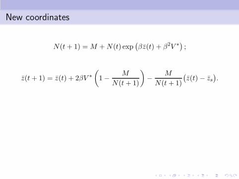
N(t+ 1) =M +N(t) exp(βz(t) + β2V ∗
);
z(t+ 1) = z(t) + 2βV ∗
(
1− M
N(t+ 1)
)
− M
N(t+ 1)
(z(t)− zs
).
New coordinates
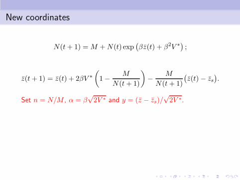
N(t+ 1) =M +N(t) exp(βz(t) + β2V ∗
);
z(t+ 1) = z(t) + 2βV ∗
(
1− M
N(t+ 1)
)
− M
N(t+ 1)
(z(t)− zs
).
Set n = N/M , α = β√2V ∗ and y = (z − zs)/
√2V ∗.
New coordinates
N(t+ 1) =M +N(t) exp(βz(t) + β2V ∗
);
z(t+ 1) = z(t) + 2βV ∗
(
1− M
N(t+ 1)
)
− M
N(t+ 1)
(z(t)− zs
).
Set n = N/M , α = β√2V ∗ and y = (z − zs)/
√2V ∗.
n(t+ 1) = 1 + n(t)Wseαy(t), y(t+ 1) = (y(t) + α)
(
1− 1
n(t+ 1)
)
,
Ws = exp(βzs + β2V ∗
)
(mean growth rate of the source population in the new conditions)
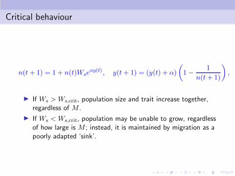
Critical behaviour
n(t+ 1) = 1 + n(t)Wseαy(t), y(t+ 1) = (y(t) + α)
(
1− 1
n(t+ 1)
)
,
◮ If Ws > Ws,crit, population size and trait increase together,regardless of M .
◮ If Ws < Ws,crit, population may be unable to grow, regardlessof how large is M ; instead, it is maintained by migration as apoorly adapted ‘sink’.
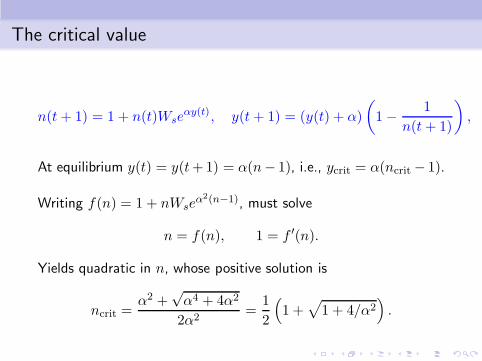
The critical value
n(t+ 1) = 1 + n(t)Wseαy(t), y(t+ 1) = (y(t) + α)
(
1− 1
n(t+ 1)
)
,
At equilibrium y(t) = y(t+1) = α(n− 1), i.e., ycrit = α(ncrit − 1).
Writing f(n) = 1 + nWseα2(n−1), must solve
n = f(n), 1 = f ′(n).
Yields quadratic in n, whose positive solution is
ncrit =α2 +
√α4 + 4α2
2α2=
1
2
(
1 +√
1 + 4/α2)
.
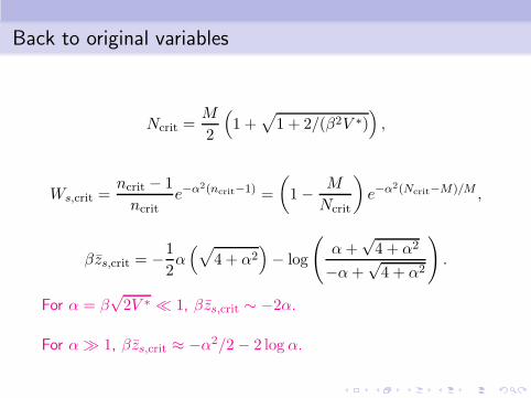
Back to original variables
Ncrit =M
2
(
1 +√
1 + 2/(β2V ∗))
,
Ws,crit =ncrit − 1
ncrite−α2(ncrit−1) =
(
1− M
Ncrit
)
e−α2(Ncrit−M)/M ,
βzs,crit = −1
2α(√
4 + α2)
− log
(
α+√4 + α2
−α+√4 + α2
)
.
For α = β√2V ∗ ≪ 1, βzs,crit ∼ −2α.
For α≫ 1, βzs,crit ≈ −α2/2− 2 log α.
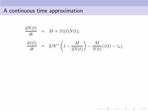
A continuous time approximation
dN(t)
dt= M + βz(t)N(t);
dz(t)
dt= 2βV ∗
(
1− M
2N(t)
)
− M
N(t)(z(t)− zs).
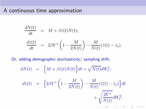
A continuous time approximation
dN(t)
dt= M + βz(t)N(t);
dz(t)
dt= 2βV ∗
(
1− M
2N(t)
)
− M
N(t)(z(t)− zs).
Or, adding demographic stochasticity/ sampling drift,
dN(t) ={
M + βz(t)N(t)}
dt+√
N(t)dW 1t ;
dz(t) ={
2βV ∗
(
1− M
2N(t)
)
− M
N(t)(z(t)− zs)
}
dt
+
√
2V ∗
N(t)dW 2
t .
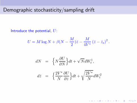
Demographic stochasticity/sampling drift
Introduce the potential, U :
U =M logN + β(N − M
2)z − M
4V ∗(z − zs)
2 .
dN ={
N∂U
∂N
}
dt+√NdW 1
t ,
dz ={2V ∗
N
∂U
∂z
}
dt+
√
2V ∗
NdW 2
t
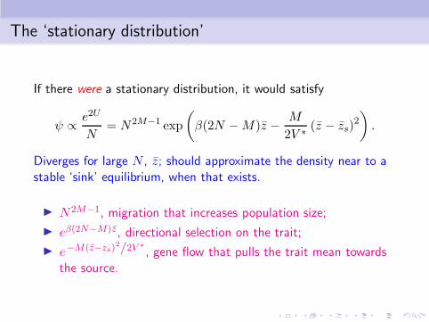
The ‘stationary distribution’
If there were a stationary distribution, it would satisfy
ψ ∝ e2U
N= N2M−1 exp
(
β(2N −M)z − M
2V ∗(z − zs)
2
)
.
Diverges for large N , z; should approximate the density near to astable ‘sink’ equilibrium, when that exists.
◮ N2M−1, migration that increases population size;
◮ eβ(2N−M)z , directional selection on the trait;
◮ e−M(z−zs)2/2V ∗
, gene flow that pulls the trait mean towardsthe source.
More on the stationary distribution
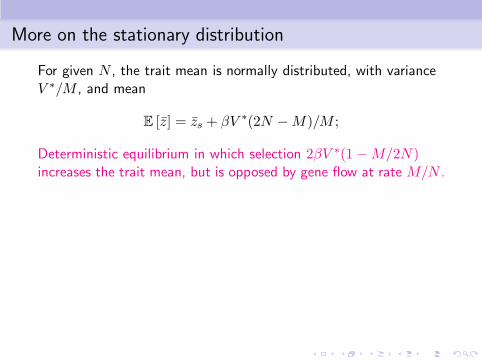
For given N , the trait mean is normally distributed, with varianceV ∗/M , and mean
E [z] = zs + βV ∗(2N −M)/M ;
Deterministic equilibrium in which selection 2βV ∗(1−M/2N)increases the trait mean, but is opposed by gene flow at rate M/N .
More on the stationary distribution
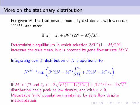
For given N , the trait mean is normally distributed, with varianceV ∗/M , and mean
E [z] = zs + βV ∗(2N −M)/M ;
Deterministic equilibrium in which selection 2βV ∗(1−M/2N)increases the trait mean, but is opposed by gene flow at rate M/N .
Integrating over z, distribution of N proportional to
N2M−1 exp
(
β2(2N −M)2V ∗
2M+ β(2N −M)zs
)
.
If M > 1/2 and zs < −2√
V ∗(1− 1/(2M)) + βV ∗/2 ∼ −2√V ∗,
distribution has a peak at low density, and with z < 0.Metastable ‘sink’ population maintained by gene flow despitemaladaptation.
Lessons from our crude analysis
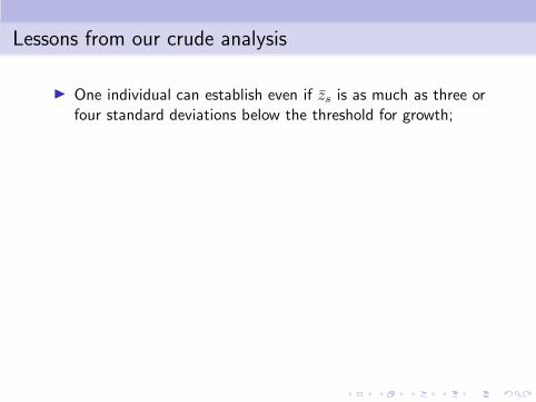
◮ One individual can establish even if zs is as much as three orfour standard deviations below the threshold for growth;
Lessons from our crude analysis
◮ One individual can establish even if zs is as much as three orfour standard deviations below the threshold for growth;
“Natural selection is a mechanism for generating an exceedinglyhigh degree of improbability.”
Lessons from our crude analysis
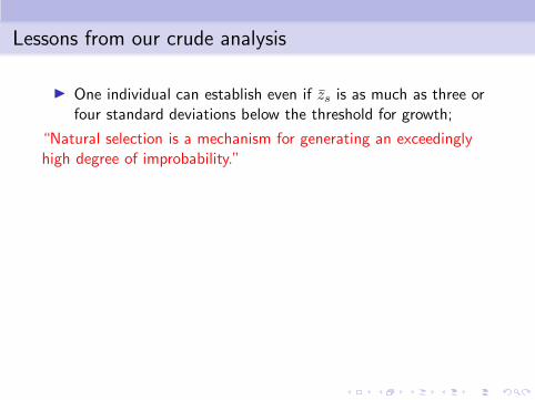
◮ One individual can establish even if zs is as much as three orfour standard deviations below the threshold for growth;
“Natural selection is a mechanism for generating an exceedinglyhigh degree of improbability.”
◮ if the mean in the source population is too low, thepopulation may be trapped in a ‘sink’;
Lessons from our crude analysis
◮ One individual can establish even if zs is as much as three orfour standard deviations below the threshold for growth;
“Natural selection is a mechanism for generating an exceedinglyhigh degree of improbability.”
◮ if the mean in the source population is too low, thepopulation may be trapped in a ‘sink’;
◮ faster migration may impede adaptation;
◮ the population can escape and adapt to a new optimum; itwill then be partially reproductively isolated (a model forspeciation in spite of gene flow);
Work of Sacha Rybaltchenko on a string of colonies strengthensthis last point, but note reduction in variance impedes ability tofurther adapt.
Top Related