SINGULARITY THEORY OF STRATEGY FUNCTIONSUNDER DIMORPHISM EQUIVALENCE

DISSERTATION

Presented in Partial Fulfillment of the Requirements for the Degree Doctor of

Philosophy in the Graduate School of the Ohio State University

By

Xiaohui Wang, MS

Graduate Program in Mathematics

The Ohio State University

2015

Dissertation Committee:

Dr. Martin Golubitsky, Advisor

Dr. Yuan Lou

Dr. King-Yeung Lam

c© Copyright by

Xiaohui Wang

2015

ABSTRACT

We study dimorphisms by applying adaptive dynamics theory and singularity

theory based on a new type of equivalence relation called dimorphism equivalence.

Dimorphism equivalence preserves ESS singularities, CvSS singularities, and dimor-

phisms for strategy functions. Specifically, we classify and compute normal forms

and universal unfoldings for strategy functions with low codimension singularities

up to dimorphism equivalence. These calculations lead to the classification of local

mutual invasibility plots that can be seen in systems of two parameters. This prob-

lem is complicated because the allowable coordinate changes are restricted to those

that preserve dimorphisms and the singular nature of strategy functions; hence the

singularity theory applied in this thesis is not a standard one.

ii

Dedicated to

Martin Golubitsky ,

and

Chunxue Cao,

for their encouragement

iii

ACKNOWLEDGMENTS

The idea of using singularity theory methods to study adaptive dynamics origi-

nated in a conversation with Ulf Dieckmann. Thanks to Odo Diekmann for bringing

up the idea of studying dimorphisms using singularity theory. Thanks to Ian Hamil-

ton for discussing the biological application of the theory developed in this thesis.

We have benefitted a lot from the discussion with Yuan Lou and Adrian Lam. This

research was supported in part by NSF Grant to DMS-1008412 to MG and NSF

Grant DMS-0931642 to the Mathematical Biosciences Institute.

iv

VITA

1986 . . . . . . . . . . . . . . . . . . . . . . . . . . . . . . . . . . Born in Chengde, China

2009 . . . . . . . . . . . . . . . . . . . . . . . . . . . . . . . . . . B.S. in Mathematics, University of Sci-ence and Technology of China

2012 . . . . . . . . . . . . . . . . . . . . . . . . . . . . . . . . . . M.S. in Mathematics, The Ohio State Uni-versity

2009-Present . . . . . . . . . . . . . . . . . . . . . . . . . . Graduate Teaching/Research Associate ,TheOhio State University

FIELDS OF STUDY

Major Field: Mathematics

Specialization: Singularity Theory, Adaptive Dynamics, Evolutionary Game Theory

v

TABLE OF CONTENTS

Abstract . . . . . . . . . . . . . . . . . . . . . . . . . . . . . . . . . . . . . . . ii

Dedication . . . . . . . . . . . . . . . . . . . . . . . . . . . . . . . . . . . . . . ii

Acknowledgments . . . . . . . . . . . . . . . . . . . . . . . . . . . . . . . . . . iv

Vita . . . . . . . . . . . . . . . . . . . . . . . . . . . . . . . . . . . . . . . . . v

List of Figures . . . . . . . . . . . . . . . . . . . . . . . . . . . . . . . . . . . viii

List of Tables . . . . . . . . . . . . . . . . . . . . . . . . . . . . . . . . . . . . xi

CHAPTER PAGE

1 Introduction . . . . . . . . . . . . . . . . . . . . . . . . . . . . . . . . . 1

1.1 Background of Adaptive Dynamics Theory . . . . . . . . . . . . . 11.2 Important Concepts in Adaptive Dynamics . . . . . . . . . . . . . 61.3 Background of Singularity Theory . . . . . . . . . . . . . . . . . . 101.4 Structure of the Thesis . . . . . . . . . . . . . . . . . . . . . . . . 15

2 Major Results and Applications . . . . . . . . . . . . . . . . . . . . . . 17

2.1 Major Results . . . . . . . . . . . . . . . . . . . . . . . . . . . . . 172.2 Application of the Theory . . . . . . . . . . . . . . . . . . . . . . . 23

3 Dimorphism equivalence . . . . . . . . . . . . . . . . . . . . . . . . . . 28

3.1 Strategy Equivalence . . . . . . . . . . . . . . . . . . . . . . . . . 283.2 Motivation of Dimorphism Equivalence . . . . . . . . . . . . . . . 313.3 Proof of Theorem 3.4 . . . . . . . . . . . . . . . . . . . . . . . . . 33

4 The Restricted Tangent Space . . . . . . . . . . . . . . . . . . . . . . . 36

4.1 A Change of Coordinates . . . . . . . . . . . . . . . . . . . . . . . 374.2 Dimorphism Equivalence Restricted Tangent Space . . . . . . . . . 374.3 Modified Tangent Space Constant Theorem . . . . . . . . . . . . . 43

vi

5 Recognition of Low Codimension Singularities . . . . . . . . . . . . . . 52

6 Universal Unfoldings under Dimorphism Equivalence . . . . . . . . . . 88

6.1 Preliminary Definitions . . . . . . . . . . . . . . . . . . . . . . . . 886.2 Dimorphism Equivalence Tangent Space . . . . . . . . . . . . . . . 906.3 Universal Unfoldings of Low Codimension Singularities . . . . . . . 91

7 The Recognition Problem for Universal Unfoldings . . . . . . . . . . . . 96

8 Geometry of Universal Unfoldings . . . . . . . . . . . . . . . . . . . . . 104

8.1 Singularities of a Strategy Function . . . . . . . . . . . . . . . . . 1048.2 Transition Variaties . . . . . . . . . . . . . . . . . . . . . . . . . . 1078.3 Mutual Invasibility Plots . . . . . . . . . . . . . . . . . . . . . . . 109

Bibliography . . . . . . . . . . . . . . . . . . . . . . . . . . . . . . . . . . . . 131

vii

LIST OF FIGURES

FIGURE PAGE

1.1 MIPs of the universal unfolding function H = ((x− y)2 + a)(x− y)2 +(x + y)(x − y). In this example the transition from a < 0 to a > 0causes the emergence of two regions of coexistence (in the right plot).Note that the evolutionary and convergence stability of the singularity(0, 0) do not change when the parameter a is varied. . . . . . . . . . 13

2.1 The MIPs of strategy function F = (w + µuv) for different values of µ. 20

2.2 The MIPs of strategy function F = −(w+µuv) for different values of µ. 20

2.3 MIPs of F = ε((δw + a)w + uv) when: (a) ε = 1, δ = 1; (b) ε = 1,δ = −1; (c) ε = −1, δ = 1; (d) ε = −1, δ = −1. In each scenarioof (ε, δ), we can see emergence of new regions at one direction of theparameter change. . . . . . . . . . . . . . . . . . . . . . . . . . . . . 21

2.4 MIPs of F = (ε+µu)w+(a+δu2)v when: (a) ε = 1, δ = 1; (b) ε = −1,δ = 1; (c) ε = 1, δ = −1; (d) ε = −1, δ = −1. In each scenario, wesee emergence of additional singularity in one direction of parameterchange while no singularities in the other direction. . . . . . . . . . . 22

3.1 Strategy functions f and g are strategy equivalent, but have differentdimorphism properties because f has regions of coexistence, whereasg does not. . . . . . . . . . . . . . . . . . . . . . . . . . . . . . . . . 29

8.1 Classification of singular points modified from Figure 2 in [10]. Basedon the evolutionary stability, convergence stability, existence of dimor-phisms, and resistance to invasion, we can divide (fxx, fyy)–space into8 separate regions. Note that each region has a sample plot. In thisplot, the curves are that of f(x, y) = 0 and the shaded areas are thosesatisfying f(x, y) > 0. . . . . . . . . . . . . . . . . . . . . . . . . . . 106

viii

8.2 MIPs of F = (−1 + µu)w + (a − u2)v when: (a) µ < 0; (b) µ = 0;(c) µ > 0. Note that the modal parameter µ only rotates the axis ofthe parabola F . However, it does not change the paired signs of eachregions and the stability of the singularities. . . . . . . . . . . . . . 111

8.3 The transition variety for F = (a + bw + w2)w + uv are a = 0 andb2 − 4a = 0. . . . . . . . . . . . . . . . . . . . . . . . . . . . . . . . . 113

8.4 MIPs of F = (a+ bw + w2)w + uv for different parameter values. . . 113

8.5 The transition variety of F = εw + (a+ bu+ δu3 + µu5)v when µ = 0is 27a2 + 4δb3 = 0. . . . . . . . . . . . . . . . . . . . . . . . . . . . . 115

8.6 MIPs of F = w + (a+ bu+ u3)v for different parameter values. . . . 115

8.7 The modal parameter space (α, β) for F = ε((a+u)w+(b+αw+βu2)v).Red curves are the non-degeneracy conditions in Theorem 6.9; bluecurves are the degenerate cases (i), (ii), (iii) summarized in previousparagraphs. (Note that only the α > 0 half plane is numbered.) . . . 118

8.8 Transition varieties of F = ε((a+u)w+ (b+αw+ βu2)v) for differentregions in the modal parameters space (α, β) when ε = 1, α > 0. Blueis variety B; Red is variety D ; Green is variety E ; Magenta is varietyN ; Black is variety C . . . . . . . . . . . . . . . . . . . . . . . . . . 119

8.9 MIPs for all the non-degenerate perturbation of F = (a+ εu)w+ (b+αw + βu2)v when {α, β} are in regions corresponding to A1 to A3. . 120

8.10 MIPs for all the non-degenerate perturbation of F = (a+ εu)w+ (b+αw + βu2)v when {α, β} are in regions corresponding to A4 to A6. . 121

8.11 MIPs for all the non-degenerate perturbation of F = (a+ εu)w+ (b+αw + βu2)v when {α, β} are in regions corresponding to A7 to A8. . 122

8.12 MIPs for all the non-degenerate perturbation of F = (a+ εu)w+ (b+αw + βu2)v when {α, β} are in regions corresponding to B1 to B3. . . 123

8.13 MIPs for all the non-degenerate perturbation of F = (a+ εu)w+ (b+αw + βu2)v when {α, β} are in regions corresponding to B4 to B6. . . 124

8.14 MIPs for all the non-degenerate perturbation of F = (a+ εu)w+ (b+αw + βu2)v when {α, β} are in regions corresponding to B7 to A9. . . 125

8.15 MIPs for all the non-degenerate perturbation of F = (a+ εu)w+ (b+αw + βu2)v when {α, β} are in regions corresponding to B10. . . . . 126

8.16 MIPs for all the non-degenerate perturbation of F = (a+ εu)w+ (b+αw + βu2)v when {α, β} are in regions corresponding to C1 to C3. . . 127

ix

8.17 MIPs for all the non-degenerate perturbation of F = (a+ εu)w+ (b+αw + βu2)v when {α, β} are in regions corresponding to C4 to C6. . . 128

8.18 MIPs for all the non-degenerate perturbation of F = (a+ εu)w+ (b+αw + βu2)v when {α, β} are in regions corresponding to C7 to C9. . . 129

8.19 MIPs for all the non-degenerate perturbation of F = (a+ εu)w+ (b+αw + βu2)v when {α, β} are in regions corresponding to C10 to C12. . 130

x

LIST OF TABLES

TABLE PAGE

2.1 The normal forms, defining and non-degeneracy conditions, and uni-versal unfoldings of singularities up to topological codimension one forstrategy functions f with a singular strategy at (0, 0). Derivatives inthe table are evaluated at the singularity (0, 0). Information aboutsingularities of topological codimension two can be found in Table 5.1and Table 6.1. (Def = defining conditions. ND = non-degeneracyconditions. TC = topological codimension.) . . . . . . . . . . . . . . 18

2.2 Markers for different singularity types on the MIPs. . . . . . . . . . . 19

2.3 The hawk-dove game . . . . . . . . . . . . . . . . . . . . . . . . . . . 25

5.1 Solution to recognition problems for singularities up to topologicalcodimension two for strategy functions f with a singular strategy at(0, 0). (Def = defining conditions. ND = non-degeneracy conditions.TC = topological codimension. ∆ = q2

u(qupww − puqww) + q2w(qupuu −

puquu)− 2quqw(qupuw − puquw)) . . . . . . . . . . . . . . . . . . . . . 53

5.2 The dimorphism equivalence restricted tangent space for the singu-larities up to topological codimension two. (TC = topological codi-mension. RT (h) = dimorphism equivalence restricted tangent spaceof h.) . . . . . . . . . . . . . . . . . . . . . . . . . . . . . . . . . . . 85

6.1 The universal unfoldings and dimorphism equivalence tangent spacefor the low codimension singularities in Theorem 6.7. (Def = defin-ing conditions. ND = non-degeneracy conditions. TC = topologicalcodimension.) . . . . . . . . . . . . . . . . . . . . . . . . . . . . . . . 92

xi

CHAPTER 1

INTRODUCTION

The application of game theory to biology has a long history. Evolutionary Game

Theory studies the evolution of phenotypic traits and was originated by Maynard-

Smith and Price [17] in 1973. Since then, there has been an explosion of interest in

evolutionary game theory by mathematicians and other scientists. Adaptive Dynam-

ics is a set of techniques and methods that studies the long-term consequences of

phenotypes by small mutations in the genotypes. In the past twenty years, adaptive

dynamics has been studied by many people, including Dieckmann and Law [5], Geritz

et al. [10], Diekmann [7], Dieckmann and Metz et al. [4], Derole and Rinaldi [3], Pole-

chova and Barton [18], and Waxman and Gavrilets [19]. Golubitsky and Vutha [14]

applied singularity theory and adaptive dynamics theory to study the ESS and CvSS

singularities of strategy functions. This thesis expands their research to further study

the dimorphisms of strategy functions.

1.1 Background of Adaptive Dynamics Theory

In this section, we briefly introduce the background of evolutionary game theory and

adaptive dynamics theory.

1

Evolutionary Game Theory

In evolutionary theory, changes in the environment are often reflected by the changes

in the residents’ ability to reproduce. Organisms that can adapt better normally have

higher reproductive rates. In biology, the individual’s ability to adapt (or reproduce)

is called fitness. Mathematical models define fitness in terms of reasonable biological

assumptions that are encoded in strategy functions. The simplest game in evolution

is a two-player single trait game. In this case, a strategy function is a real-valued

function f(x, y) where x and y are the strategies or (phenotypes) of the players (or

organisms). A strategy function f(x, y) represents the fitness advantage of a mutant

with phenotype y when competing against a resident with phenotype x. In game

theory, f(x, y) > 0 means that the mutant has a fitness advantage over the resident.

Since any strategy has 0 advantage against itself, we define

Definition 1.1. The smooth function f : R × R → R is a strategy function if

f(x, x) = 0 for all x.

Remark 1.2. Since a strategy function f vanishes along the diagonal (x, x), we can

see by direct calculation that certain derivatives of f also vanish along the diagonal.

For example,

fx + fy = 0

fxx + 2fxy + fyy = 0

· · ·

at (x, x) for all x.

2

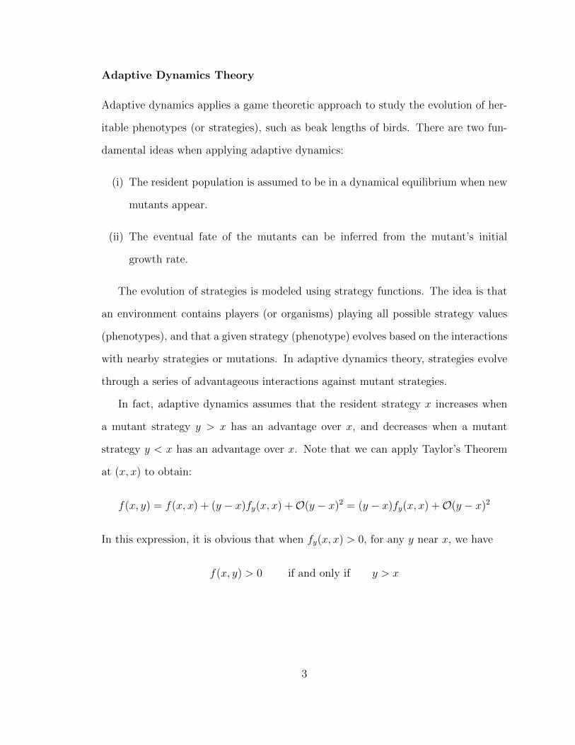
Adaptive Dynamics Theory

Adaptive dynamics applies a game theoretic approach to study the evolution of her-

itable phenotypes (or strategies), such as beak lengths of birds. There are two fun-

damental ideas when applying adaptive dynamics:

(i) The resident population is assumed to be in a dynamical equilibrium when new

mutants appear.

(ii) The eventual fate of the mutants can be inferred from the mutant’s initial

growth rate.

The evolution of strategies is modeled using strategy functions. The idea is that

an environment contains players (or organisms) playing all possible strategy values

(phenotypes), and that a given strategy (phenotype) evolves based on the interactions

with nearby strategies or mutations. In adaptive dynamics theory, strategies evolve

through a series of advantageous interactions against mutant strategies.

In fact, adaptive dynamics assumes that the resident strategy x increases when

a mutant strategy y > x has an advantage over x, and decreases when a mutant

strategy y < x has an advantage over x. Note that we can apply Taylor’s Theorem

at (x, x) to obtain:

f(x, y) = f(x, x) + (y − x)fy(x, x) +O(y − x)2 = (y − x)fy(x, x) +O(y − x)2

In this expression, it is obvious that when fy(x, x) > 0, for any y near x, we have

f(x, y) > 0 if and only if y > x

3

Therefore, we can see a proportional relationship between the rate of change of strate-

gies in evolution and the mutation gradient fy(x, x) of the fitness function f . Dieck-

mann and Law [5] have applied this approach and obtained the canonical equation of

adaptive dynamics:

dx

dt= α(x)fy(x, x) (1.1.1)

where α(x) > 0 depends on the resident strategy x.

From the canonical equation of adaptive dynamics, we see that (1.1.1) has an

equilibrium at x0 if and only if fy(x0, x0) = 0. Therefore, we define

Definition 1.3. A strategy x0 is a singular strategy if fy(x0, x0) = 0.

An Example of a Fitness Function

In the simplest case, we assume that the resident population initially consists of asex-

ual organisms that all possess the same phenotype x (also known as a monomorphic

population). We also assume that y is the phenotype of the rare mutations and that

the fitness function is f(x, y).

Mutations that differ from the resident are randomly and recurrently generated,

and these can be thought of attempting to invade the resident. In this context, f can

be defined in terms of a population growth rate k (see (1.1.5)).

We now introduce k for monomorphic populations, show how k leads to growth

rates for a system of two populations with different phenotypes (see (1.1.4)), and

show that the stability of the populations are given in terms of k (see Theorem 1.4).

To define k, suppose that w is the size of a monomorphic population with phe-

notype x. Assume that the growth rate of the population is determined by the

population and the trait value. That is:

w = k(w, x)w (1.1.2)

4

where k(w, x) is smooth, and · is the derivative of w with respect to time.

Since the population is monomorphic, we can assume that there is a zero of k(w, x)

for each x (defined locally near a given x0) denoted by (p(x), x) where p(x) > 0 is

smooth. That is,

k(p(x), x) ≡ 0 (1.1.3)

This equilibrium is assumed to be stable for (1.1.2) near the given x0, that is,

kw(p(x0), x0) < 0

When there is more than one phenotype in the system, the growth rate for each

phenotype is assumed to be determined by the trait value of this phenotype and the

total population of all phenotypes. In particular, when there are two phenotypes,

suppose that the resident x has a population u and the mutant y has a population v,

then the population equations have the form

u = uk(u+ v, x)

v = vk(v + u, y)(1.1.4)

Note that (p(x), 0, x, y) is an equilibrium of (1.1.4) where the mutant population is

zero and the resident population is p(x). In this case, the growth rate of the mutant

is k(p(x), y) and the fitness function of rare mutations with phenotype y in a resident

population with phenotype x is

f(x, y) = k(p(x), y) (1.1.5)

where x is near x0. Equation (1.1.3) implies that

f(x, x) = k(p(x), x) = 0

Theorem 1.4. The equilibrium (p(x), 0, x, y) of (1.1.4) is unstable if f(x, y) > 0 and

stable if f(x, y) < 0.

5

Proof. The Jacobian J(u, v, x, y) for the system (1.1.4) isk(u+ v, x) + ukw(u+ v, x) ukw(u+ v, x)

vkw(v + u, y) k(v + u, y) + vkw(v + u, y)

(1.1.6)

At the equilibrium point (p(x), 0, x, y), the Jacobian becomes

J(u, v, x, y)|(p(x),0,x,y) =

p(x)kw(p(x), x) p(x)kw(p(x), x)

0 k(p(x), y)

(1.1.7)

We know from the assumptions of k(w, x) that

p(x) > 0 kw(p(x), x) < 0

Therefore, we have

p(x)kw(p(x), x) < 0

Thus, the stability of the equilibrium (p(x), 0, x, y) is determined by the sign of

k(p(x), y). The proof is complete by recalling (1.1.5).

Remark 1.5. Theorem 1.4 shows that the stability of the equilibrium is determined

by the signs of the fitness function f(x, y). This is consistent with the definition

of fitness function; that is, f(x, y) < 0 indicates that the mutant has no advantage

against the resident. This is the same as saying that the resident population stays in

a stable equilibrium. Moreover, the population with phenotype y will gradually die

out, and the system will remain monomorphic.

On the contrary, if f(x, y) > 0 then the mutant has an advantage over the resident.

Moreover, the resident population is unstable and will be invaded by the mutant.

Thus, the population with phenotype y will increase.

1.2 Important Concepts in Adaptive Dynamics

Next we introduce three important concepts from adaptive dynamics.

6

ESS

An evolutionarily stable strategy (ESS) is a resident phenotype (i.e. strategy x) such

that no mutant with phenotype y near x can invade the resident. That is, f(x, y) ≤ 0

for all y near x. Considering that f(x, x) = 0 for all x, it is necessary to have that

fy(x, x) = 0 and fyy(x, x) ≤ 0. Specifically:

Definition 1.6. x is an ESS if

fx(x, x) = 0 fyy(x, x) < 0

Remark 1.7. Remark 1.2 implies that fx(x, x) = 0 if and only if fy(x, x) = 0.

CvSS

A convergence stable strategy (CvSS) is a phenotype (i.e. strategy x) such that it

is a linearly stable equilibrium in x for the canonical equation of adaptive dynamics

(1.1.1). If a phenotype x is a CvSS singularity, it is actually a local attractor in

adaptive dynamics. This means, any nearby resident strategy will follow the canonical

equation of adaptive dynamics and evolve towards to direction of x. Recall that x is

a linearly stable equilibrium of (1.1.1) if

fy(x, x) = 0d

dx(α(x)fy(x, x))|x=x < 0

By Remark 1.2, we have

d

dx(α(x)fy(x, x))|x=x = α′(x)fy(x, x) + α(x)(fxy(x, x) + fyy(x, x))

=1

2α(x)(fyy(x, x)− fxx(x, x))

Since α(x) > 0 for all x, we have

Definition 1.8. x is a CvSS if

fx(x, x) = 0 fyy(x, x)− fxx(x, x) < 0

7

Dimorphism and Region of Coexistence

Adaptive dynamics theory attempts to predict phenotypic evolutionary change. In

the long run of evolution, either mutations die out or they do not die out. If the

mutant with phenotype y has no advantage over the resident with phenotype x (i.e.

f(x, y) < 0), the mutant will die out. On the other hand, if the mutant with pheno-

type y has an advantage over the resident with phenotype x (i.e. f(x, y) > 0), then

the mutant’s population will grow and they will not die out. However, in some situ-

ations, the mutant cannot outcompete the resident once the resident is rare and we

get coexistence of two subpopulations with different phenotypes. That is, the system

becomes a dimorphic population. This happens when f(x, y) > 0 and f(y, x) > 0

and such a pair of phenotypes is called a dimorphism. So we have

Definition 1.9. Let f(x, y) be a strategy function. A pair of strategies x, y that

satisfies

f(x, y) > 0 f(y, x) > 0

is called a dimorphism of f . The set of all dimorphisms of f is called the region of

coexistence.

Remark 1.10. There is a sufficient condition for the local existence of dimorphisms:

If fx(x, x) = 0 and fyy(x, x)+fxx(x, x) > 0, then there exists pairs of strategies (x, y)

near (x, x) such that both f(x, y) > 0 and f(y, x) > 0.

Proof. Let g(x) = f(x, 2x − x), we claim that g(x) > 0 when x is close to x. We

know

g′(x) = fx(x, 2x− x)− fy(x, 2x− x)

g′′(x) = fxx(x, 2x− x)− 2fxy(x, 2x− x) + fyy(x, 2x− x)

. . .

8

where ′ is derivative with respect to x. Then, we have

g(x) = g(x) + g′(x)(x− x) +1

2g′′(x)(x− x)2 + h.o.t,

From Remark 1.2, we know

g(x) = f(x, x) = 0

g′(x) = fx(x, x)− fy(x, x) = 0

g′′(x) = 2(fxx(x, x) + fyy(x, x)) > 0

Therefore, we can conclude that when x is close to x

g(x) =1

2g′′(x)(x− x)2 + h.o.t > 0

Note that (x, 2x − x) and (2x − x, x) are symmetrical about (x, x). With similar

calculations we also have

g(2x− x) = g′′(x)(x− x)2 + h.o.t > 0

That is to say,

f(x, 2x− x) > 0 f(2x− x, x) > 0

Hence, (x, 2x− x) are pairs of dimorphisms around the singular point (x, x) when x

is close to x.

Remark 1.11. In some of the literature of adaptive dynamics, dimorphism is also

referred to as mutual invasibility. Diekmann [7] discussed the consequence of mutual

invasibility. It is found that

• If there is a dimorphism (x, y) near a singular strategy x that is both an ESS and

a CvSS, then both strategies x and y will evolve towards x, and this dimorphism

(x, y) is called a converging dimorphism.

9

• If there is a dimorphism (x, y) near a singular strategy x that is a CvSS, but

not an ESS, then we can observe an interesting phenomenon called evolutionary

branching. When this happens, (x, y) is is called a diverging dimorphism. Some

detailed discussion about evolutionary branching can be found in [15, 9, 16].

In this thesis we will keep track of dimorphism pairs, but not explicitly of converging

and diverging dimorphisms.

1.3 Background of Singularity Theory

In this section, we discuss the general ideas of singularity theory and how it helps

in studying ESS singularities, CvSS singularities and dimorphisms in the context

of adaptive dynamics. In addition, we introduce mutual invasibility plots which

show how ESS, CvSS, and dimorphisms can interact. At the end, we introduce the

classification of singularities by topological codimension.

Standard Singularity Theory and its Applications

Singularity theory studies how a certain local property of a class of functions changes

as parameters are varied. The important first step when trying to apply singularity

theory is to determine transformations of functions that preserve the property that

one is trying to study. We will use a series of examples to explain this.

1. In the simplest case, the property to be studied is the zero sets of functions

f : Rn → Rn near a given zero. We define:

Definition 1.12. Two functions f, g : Rn → Rn are contact equivalent if there

exists a function S : Rn → R and a coordinate change Φ : Rn → Rn such that

g(x) = S(x)f(Φ(x))

10

where S(x) > 0 and Φ : Rn → Rn is a near identity diffeomorphism.

It is easy to see that the contact equivalence (S,Φ) transforms the zero set of g

to the zero set of f .

2. Golubitsky and Vutha [14] study the ESS and CvSS singularities of strategy

functions. They develop an equivalence relation called strategy equivalence (see

Definition 3.1) to preserve these singularities among strategy functions.

3. This thesis studies the transformations that preserve dimorphisms as well as

ESS and CvSS singularities of strategy functions. We construct a modified

version of strategy equivalence called dimorphism equivalence (See Definition

3.3) such that it preserves these three properties of strategy functions.

In singularity theory, a singularity is a transition point where the property one

studies changes. For example, in the study of the zero set of a function f , a singularity

is a point x such that f(x) = 0 and (Df)x is singular. That is, the transition point

when the number of zeroes of f changes. In the case of studying dimorphism, ESS,

and CvSS simultaneously, a singularity will be a transition point where at least one

of these three properties changes.

Once one has established the most general equivalence relation that preserves

these properties, it is natural to ask when is a function f equivalent to a specific

function h on a neighborhood of a singularity? This question is called the recognition

problem. The specific function h is called the normal form and is usually the ‘simplest

representative’ from the whole equivalence class of h. A major result of singularity

theory is that the recognition problem can be solved by examining a finite number of

derivatives of f at the singularity point. For example:

11

Theorem 1.13. Assume that a strategy function f(x, y) has a singularity at (0, 0).

Then f is dimorphism equivalent to

h = (x− y)4 + (x+ y)(x− y)

if and only if at (0, 0)

fx = 0 fxy = 0

fxx > 0 fxx(fx4 + 6fx2y2 + fy4)− 4(fx2y + fxy2)(3fxy2 + fy3) > 0

In the theorem for a recognition problem, the equalities are called defining condi-

tions, the inequalities are called non-degeneracy conditions.

Singularity theory studies the key properties of small perturbations of a given

function f by applying universal unfolding theory. An unfolding of a function f is

a parametrized family F (x, α) such that F (x, 0) = f where α ∈ Rk is a parame-

ter. A versal unfolding of f contains all small perturbations of f up to the general

equivalence. A universal unfolding of f is a versal unfolding with the smallest k.

Once a singularity is identified in a normal form h, we can find all possible small

perturbations of h in its universal unfolding H(x, α) up to equivalence. For example:

Theorem 1.14. A universal unfolding of h = (x− y)4 + (x+ y)(x− y) is

H = ((x− y)2 + a)(x− y)2 + (x+ y)(x− y)

where a is a parameter near 0.

The techniques needed to prove Theorem 1.14 follow from those needed to solve

the recognition problem in Theorem 1.13. With universal unfolding theory, we are

able to classify all small perturbations of a strategy function f up to dimorphism

equivalence.

12

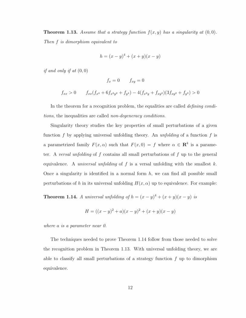
Geometry and Mutual Invasibility Plots

Another benefit of universal unfolding theory is that it helps study the geometry

of small perturbations around singularities. For a given strategy function we use

mutual invasibility plots (MIPs) to illustrate ESS and CvSS singularities, and regions

of coexistence. For example, Figure 1.1 shows the two possible perturbations of the

strategy function h = (x−y)4+(x+y)(x−y) up to dimorphism equivalence by plotting

the data for the universal unfolding H = ((x− y)2 + a)(x− y)2 + (x + y)(x− y) for

a > 0 and a < 0. In these plots, the blue curve is H(x, y, a) = 0, the red curve is

H(y, x, a) = 0, and the black curve is the line y = x. In each region, we can see a

pair of signs and they stand for sgn(H(x, y, a)) and sgn(H(y, x, a)). The centered red

dot stands for a singularity that is both ESS and CvSS. Plots like these are called

mutual invasibility plots (MIPs).

+−

−−

−−

+−

−+

−+

a < 0

−+

−+

+−

+−

−−

−−

a = 0

+−

−+

++

++

−+

+−

−−

−−

a > 0

Figure 1.1: MIPs of the universal unfolding function H = ((x−y)2 +a)(x−y)2 +(x+

y)(x − y). In this example the transition from a < 0 to a > 0 causes the emergence

of two regions of coexistence (in the right plot). Note that the evolutionary and

convergence stability of the singularity (0, 0) do not change when the parameter a is

varied.

13

In Figure 1.1, we see that regions of coexistence can emerge from the perturbation

of a singular strategy function. The MIP for the singular strategy function h is the

middle plot of Figure 1.1. There is no region of coexistence in the middle plot.

However, if we perturb the parameter to a > 0 (as in the right plot), the strategy

function has two regions of coexistence; whereas, when a < 0 (as in the left plot), the

strategy function has no region of coexistence. We can think of this singular strategy

as creating regions of coexistence.

Remark 1.15. In the adaptive dynamics literature, there is another useful plot

called a pairwise invasibility plot (PIP). For any strategy function f , a PIP contains

the curve f(x, y) = 0 and sgn(f) in each region bounded by f(x, y) = 0.

Classification of Singularities

In this thesis we solve the recognition problems, find the universal unfoldings, and

plot the MIPs (for all perturbations up to dimorphism equivalence) for singularities of

topological codimension ≤ 2. In specific, Theorem 5.1 classifies all such singularities,

Theorem 6.9 gives the universal unfoldings for these singularities, and Chapter 8

contains MIPs for all possible perturbations. The results for topological codimension

one are much simpler and they are presented in Chapter 2.

Codimension

Next, we explain what codimension is. For a strategy function f with a given singular-

ity, the universal unfolding F (x, α) contains all perturbations of f up to dimorphism

equivalence. The C∞ codimension of f is the number of parameters in the univer-

sal unfolding F . The parameters in universal unfoldings are often called unfolding

parameters.

Suppose that the perturbations of f associated with a parameter β, that is F (·, β),

14

have constant C∞ codimension and the functions are not equivalent for different β.

Then we call the parameter β a modal parameter. Golubitsky and Schaeffer [12]

define the topological codimension of a function f as its C∞ codimension minus the

number of modal parameters in a universal unfolding of f . Therefore, as is standard

in singularity theory, we can classify singularities of strategy functions up to a given

C∞ or topological codimension. We choose ‘topological codimension’ because this

is the number of parameters that are needed in an application for the particular

singularity to be able to occur generically.

1.4 Structure of the Thesis

In Chapter 2, we summarize the major results of this thesis and provide an appli-

cation of our theory. In Chapter 3 we review Golubitsky and Vutha’s [14] strategy

equivalence and introduce dimorphism equivalence which preserves ESS and CvSS

singularities and dimorphisms. In Chapter 4, given a strategy function f , we present

a sufficient condition to determine all small perturbations η so that f + η is dimor-

phism equivalent to f . The result is stated in the modified tangent space constant

theorem (Theorem 4.7). In Chapter 5, we apply Theorem 4.7 to solve the recognition

problems under dimorphism equivalence for singularities of topological codimension

≤ 2. For each of these singularities we find the normal form and its defining and

non-degeneracy conditions. See Table 5.1 for details. In Chapter 6, we discuss uni-

versal unfoldings of strategy functions up to dimorphism equivalence. An important

theorem in singularity theory shows the existence of universal unfoldings and provides

methods to calculate them. We apply these methods in the context of dimorphism

equivalence and find the universal unfoldings for singularities up to topological codi-

mension two. See Table 6.1 for details. In Chapter 7, we solve the problem of when

is an unfolding universal for a given strategy function f . This result is useful when

15

determining whether a universal unfolding of a degenerate singularity is contained

in a given application. We illustrate the standard methods with a few examples. In

Chapter 8, we study the geometry of the unfolding space for each singularity up to

topological codimension two. For these singularities, we determine the MIPs of all

possible perturbations up to dimorphism equivalence.

16

CHAPTER 2

MAJOR RESULTS AND APPLICATIONS

In this chapter, we present our major results and explain why these results are im-

portant. In addition, we apply our theory to study the famous Hawk-Dove game.

2.1 Major Results

As discussed in Chapter 1, we apply adaptive dynamics theory and singularity theory

to study certain local properties (ESS singularities, CvSS singularities, and dimor-

phisms) of strategy functions. That is, we assume x0 is a singular strategy and we

determine when we have ESS singularities, CvSS singularities, and dimorphisms in

a universal unfolding of that singularity. We study all singularities up to topologi-

cal codimension two. In this section we only list the results for singularities up to

topological codimension one. The results for singularities of codimension two are

more complicated and are shown in Theorem 5.1 (normal forms) and Theorem 6.9

(universal unfoldings). Note that all results use the (u, v) coordinates

u = x+ y

v = x− y

We also denote w = v2. The (u, v) coordinates simplify the calculations in the proofs

of many of our theorems. We show in Chapter 4 that a general strategy function f

17

can be rewritten as

f = p(u,w)w + q(u,w)v

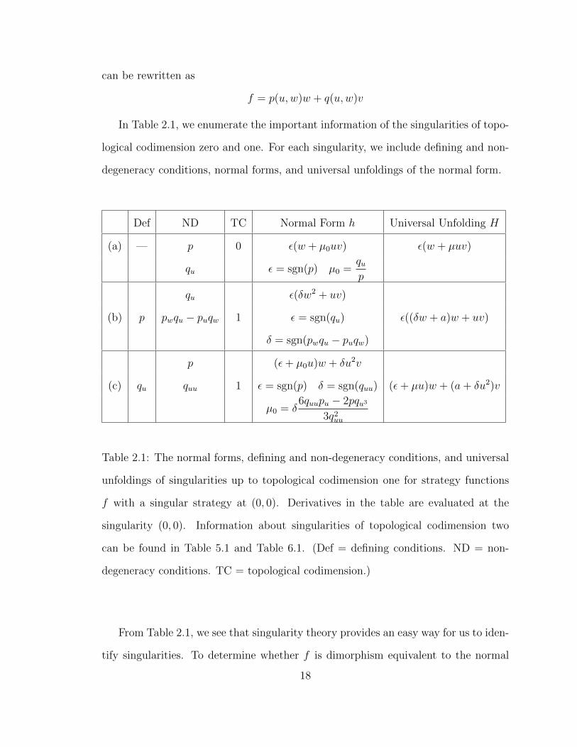
In Table 2.1, we enumerate the important information of the singularities of topo-

logical codimension zero and one. For each singularity, we include defining and non-

degeneracy conditions, normal forms, and universal unfoldings of the normal form.

Def ND TC Normal Form h Universal Unfolding H

(a) — p 0 ε(w + µ0uv) ε(w + µuv)

qu ε = sgn(p) µ0 =qup

qu ε(δw2 + uv)

(b) p pwqu − puqw 1 ε = sgn(qu) ε((δw + a)w + uv)

δ = sgn(pwqu − puqw)

p (ε+ µ0u)w + δu2v

(c) qu quu 1 ε = sgn(p) δ = sgn(quu) (ε+ µu)w + (a+ δu2)v

µ0 = δ6quupu − 2pqu3

3q2uu

Table 2.1: The normal forms, defining and non-degeneracy conditions, and universal

unfoldings of singularities up to topological codimension one for strategy functions

f with a singular strategy at (0, 0). Derivatives in the table are evaluated at the

singularity (0, 0). Information about singularities of topological codimension two

can be found in Table 5.1 and Table 6.1. (Def = defining conditions. ND = non-

degeneracy conditions. TC = topological codimension.)

From Table 2.1, we see that singularity theory provides an easy way for us to iden-

tify singularities. To determine whether f is dimorphism equivalent to the normal

18

form h, we only need to calculate certain derivatives of the strategy function f eval-

uated at the singularity point. Once we have identified the singularity, we draw the

MIPs of the universal unfolding for all possible parameter values up to dimorphism

equivalence.

Figure 2.1 to Figure 2.4 contain all possible mutual invasibility plots up to di-

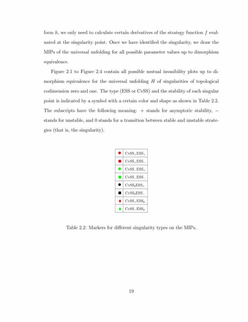
morphism equivalence for the universal unfolding H of singularities of topological

codimension zero and one. The type (ESS or CvSS) and the stability of each singular

point is indicated by a symbol with a certain color and shape as shown in Table 2.2.

The subscripts have the following meaning: + stands for asymptotic stability, −

stands for unstable, and 0 stands for a transition between stable and unstable strate-

gies (that is, the singularity).

• CvSS+ESS+

� CvSS+ESS−

• CvSS−ESS+

� CvSS−ESS−

• CvSS0ESS+

� CvSS0ESS−

� CvSS+ESS0

� CvSS−ESS0

Table 2.2: Markers for different singularity types on the MIPs.

19

++

++

−+

+−

−+

+−

(i) µ < −1

++

++

+−

−+

+−

−+

(ii) −1 < µ < 0

++

−+

+−

+−

−+

++

(iii) 0 < µ < 1

−+

−+

++

+−

+−

++

(iv) µ > 1

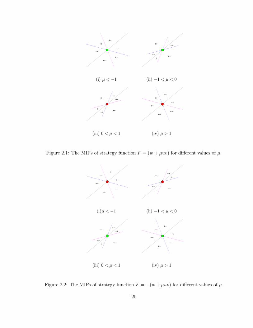
Figure 2.1: The MIPs of strategy function F = (w + µuv) for different values of µ.

−−

−−

+−

−+

+−

−+

(i)µ < −1

−−

−+

+−

−+

+−

−−

(ii) −1 < µ < 0

+−

−+

+−

−+

−−

−−

(iii) 0 < µ < 1

−+

+−

−+

−−

−−

+−

(iv) µ > 1

Figure 2.2: The MIPs of strategy function F = −(w + µuv) for different values of µ.

20

−+

−+

++

++

+−+−

−−

−−

−+

−+

+−

++

++

+−

−+

+−

−+

+−

++

++

(a) F = (w + a)w + uv: (i)a < 0, (ii) a = 0, (iii) a > 0

+−

−−

−−

+−

−+

−+

−+

−+

+−

+−

−−

−−

+−

−+

++

++

−+

+−

−−

−−

(b) F = (−w + a)w + uv: (i)a < 0, (ii) a = 0, (iii) a > 0

+−

−+

−+

+−

−−

++

++

−−

−+

−+

+−

+−−−

−− +−

+−

−+

−+

−−

−−

(c) F = −(w + a)w − uv: (i)a < 0, (ii) a = 0, (iii) a > 0

+−

+−

−+

++

++

−+

++

++

−+

−+

+−

+−

+−

−+

−+

+−

++

−−

−−

++

(d) F = −(−w + a)w − uv: (i)a < 0, (ii) a = 0, (iii) a > 0

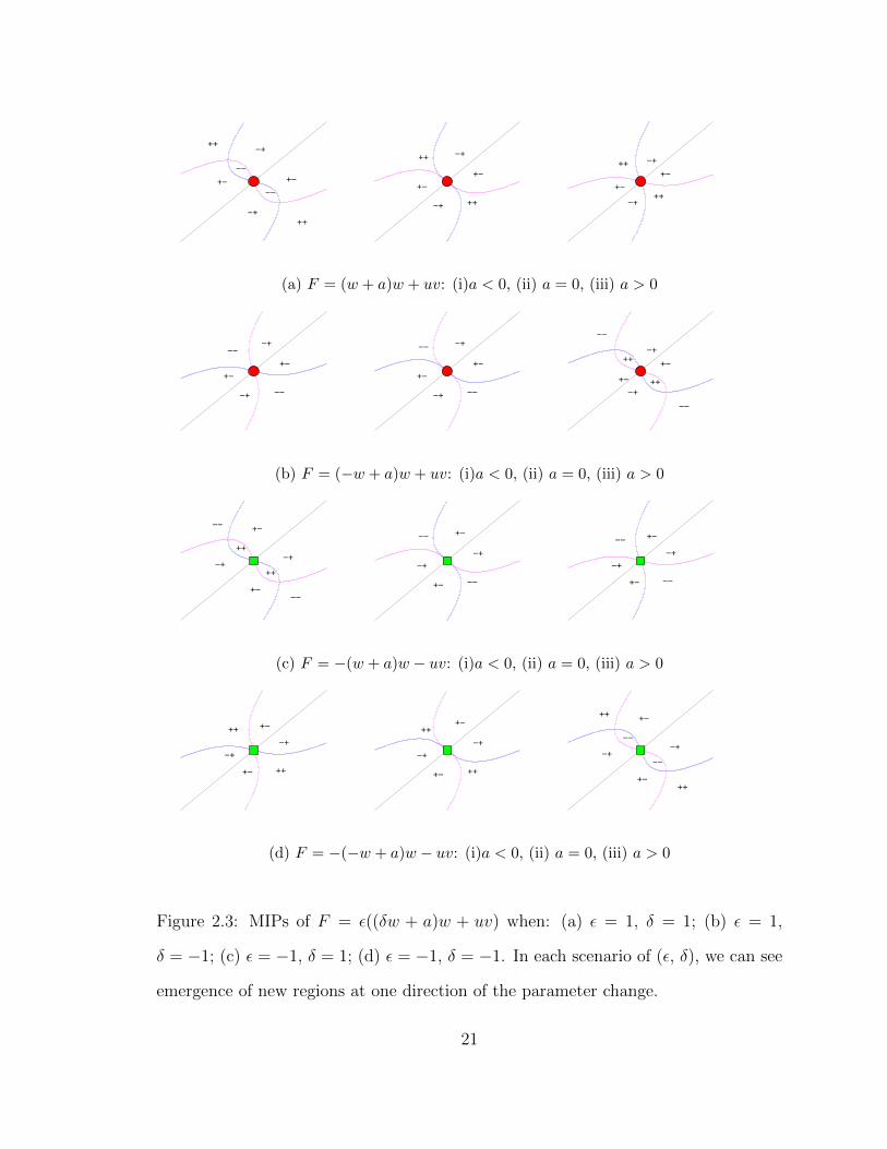
Figure 2.3: MIPs of F = ε((δw + a)w + uv) when: (a) ε = 1, δ = 1; (b) ε = 1,

δ = −1; (c) ε = −1, δ = 1; (d) ε = −1, δ = −1. In each scenario of (ε, δ), we can see

emergence of new regions at one direction of the parameter change.

21

−+

+−

+−

−+

−+

+−

++

++

++

+−

−+

−+

+−

++

++

++

+−

+−

−+

−+

(a) F = (1 + µu)w + (a+ u2)v when µ = 0: (L) a < 0, (M) a = 0, (R) a > 0

−+

+−

+−

−+

−+

+−

−−

−−

+−

−+

−+

+−−−

−−

+−

+−

−+

−+

−−

−−

(b) F = (−1 + µu)w + (a+ u2)v when µ = 0: (L) a < 0, (M) a = 0, (R) a > 0

+−

−+

+−

−+

++

++ +−

−+

+−

−+++

++

++

++

+−

−+

−+

+−

+−

−+

(c) F = (1 + µu)w + (a− u2)v when µ = 0: (L) a < 0, (M) a = 0, (R) a > 0

−−

+−

−+

+−

−+

−−

−−

−−+−

−+

+−

−+

+−

−+

−+

+−

+−

−+

−−

−−

(d) F = (−1 + µu)w + (a− u2)v when µ = 0: (L) a < 0, (M) a = 0, (R) a > 0

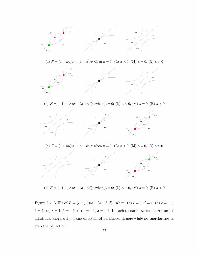
Figure 2.4: MIPs of F = (ε+ µu)w + (a+ δu2)v when: (a) ε = 1, δ = 1; (b) ε = −1,

δ = 1; (c) ε = 1, δ = −1; (d) ε = −1, δ = −1. In each scenario, we see emergence of

additional singularity in one direction of parameter change while no singularities in

the other direction.22

The MIPs of the universal unfolding of singularity (a) up to dimorphism equiva-

lence are given in Figures 2.1 and 2.2 . We see that dimorphisms only exists when

p > 0. Once sgn(p) is fixed, the difference in the modal parameter µ can change

the stability of ESS or CvSS. Up to dimorphism equivalence, there are eight different

types of MIPs for the topological codimension zero singularity.

The MIPs of the universal unfolding of singularity (b) up to dimorphism equiva-

lence are given in Figure 2.3. We see that as we vary the parameter a across 0, there

is a creation of new regions. In addition, sgn(qu) determines the ESS or CvSS singu-

larity types and corresponding stabilities. If a strategy function has this singularity,

with the help of singularity theory and these MIPs, we can predict whether we can

find pairs of dimorphisms in the perturbed strategy function and if the answer is yes,

where we can obtain pairs of dimorphisms in the parameter space.

Figure 2.4 contains the MIPs of all universal unfolding of singularity (c) up to

dimorphism equivalence when the modal parameter µ = 0. The figures show that as

we vary the parameter a, the number and stabilities of ESS and CvSS singularities

change, but the existence of regions of coexistence does not. Note that µ = 0 is a

special case of all strategy functions with singularity (c), we point out that µ = 0 is a

standard representative for the all parameter values of µ. We discuss the influence of

different values of the modal parameter µ on the topology of the MIPs in Chapter 8.

2.2 Application of the Theory

This thesis provides the theoretical support and general methodology to simulta-

neously study ESS singularities, CvSS singularities, and dimorphisms of strategy

functions. It is usually extremely difficult to study the properties of a general strat-

egy function f and its perturbations. By developing an equivalence relation (i.e.

23

dimorphism equivalence) that preserves ESS singularities, CvSS singularities, and di-

morphisms, we find the conditions for a class of strategy functions to be dimorphism

equivalent to singularities up to topological codimension two. This theory hugely

simplifies the calculations in identifying the singularities. The universal unfolding

theory allows us to study the key properties of all perturbations of a given strategy

function. Since a class of strategy functions that are dimorphism equivalent share the

same key properties in their corresponding perturbations up to dimorphism equiv-

alence, we only need to study a representative (usually the normal form) from this

class. The MIPs in Chapter 8 show all key properties for the universal unfoldings of

each singularity up to topological codimension 2. Within each plot, ESS singularities,

CvSS singularities, and dimorphisms are given specifically. Therefore, with the help

of our theory and the MIPs, we can easily tell whether dimorphisms exist if one is

studying an evolutionary problem with a specific fitness function.

In particular, to apply our theory, we look at the famous Hawk-Dove example in

evolutionary theory.

The Hawk Dove Game

Dieckmann and Metz [6] considered generalizations of the classical Hawk-Dove game

that lead to strategy functions. Golubitsky and Vutha [14] study this game in the

context of strategy equivalence and find different types of ESS and CvSS singularities

as parameters are varied.

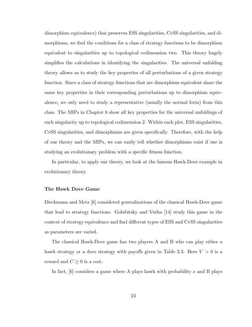
The classical Hawk-Dove game has two players A and B who can play either a

hawk strategy or a dove strategy with payoffs given in Table 2.3. Here V > 0 is a

reward and C ≥ 0 is a cost.

In fact, [6] considers a game where A plays hawk with probability x and B plays

24

Hawk Dove

Hawk1

2(V − C) V

Dove 01

2V

Table 2.3: The hawk-dove game

hawk with probability y. Dieckmann and Metz [6] show that the advantage for B in

this game is given by the strategy function

f(x, y) = (y − x)(V − Cx) (2.2.1)

Dieckmann and Metz [6] also consider variations of (2.2.1) that lead to parametrized

families of strategy functions, which are based on various ecological assumptions (See

[6] for details). Their most complicated game has the form

f(x, y) = ln(1 +Q(x, y)

1 +Q(x, x)) (2.2.2)

where

P (x) = r0 + r1(x− x0) + r2(x− x0)2

A(x, y) =1

2

√P (x)P (y)

B(x, y) = V (1− x+ y)− Cxy

Q(x, y) = A(x, y)B(x, y)/R

(2.2.3)

Based on certain biological explanation of the parameters, we also assume that in

(2.2.3)

R > 0 C > 0 V > 0

Example 2.1. By applying our singularity theory results we show that the fitness

25

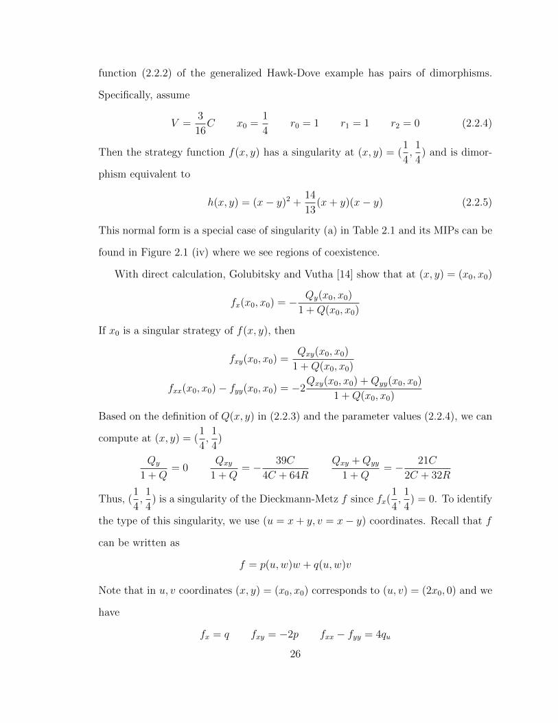
function (2.2.2) of the generalized Hawk-Dove example has pairs of dimorphisms.

Specifically, assume

V =3

16C x0 =

1

4r0 = 1 r1 = 1 r2 = 0 (2.2.4)

Then the strategy function f(x, y) has a singularity at (x, y) = (1

4,1

4) and is dimor-

phism equivalent to

h(x, y) = (x− y)2 +14

13(x+ y)(x− y) (2.2.5)

This normal form is a special case of singularity (a) in Table 2.1 and its MIPs can be

found in Figure 2.1 (iv) where we see regions of coexistence.

With direct calculation, Golubitsky and Vutha [14] show that at (x, y) = (x0, x0)

fx(x0, x0) = − Qy(x0, x0)

1 +Q(x0, x0)

If x0 is a singular strategy of f(x, y), then

fxy(x0, x0) =Qxy(x0, x0)

1 +Q(x0, x0)

fxx(x0, x0)− fyy(x0, x0) = −2Qxy(x0, x0) +Qyy(x0, x0)

1 +Q(x0, x0)

Based on the definition of Q(x, y) in (2.2.3) and the parameter values (2.2.4), we can

compute at (x, y) = (1

4,1

4)

Qy

1 +Q= 0

Qxy

1 +Q= − 39C

4C + 64R

Qxy +Qyy

1 +Q= − 21C

2C + 32R

Thus, (1

4,1

4) is a singularity of the Dieckmann-Metz f since fx(

1

4,1

4) = 0. To identify

the type of this singularity, we use (u = x+ y, v = x− y) coordinates. Recall that f

can be written as

f = p(u,w)w + q(u,w)v

Note that in u, v coordinates (x, y) = (x0, x0) corresponds to (u, v) = (2x0, 0) and we

have

fx = q fxy = −2p fxx − fyy = 4qu

26

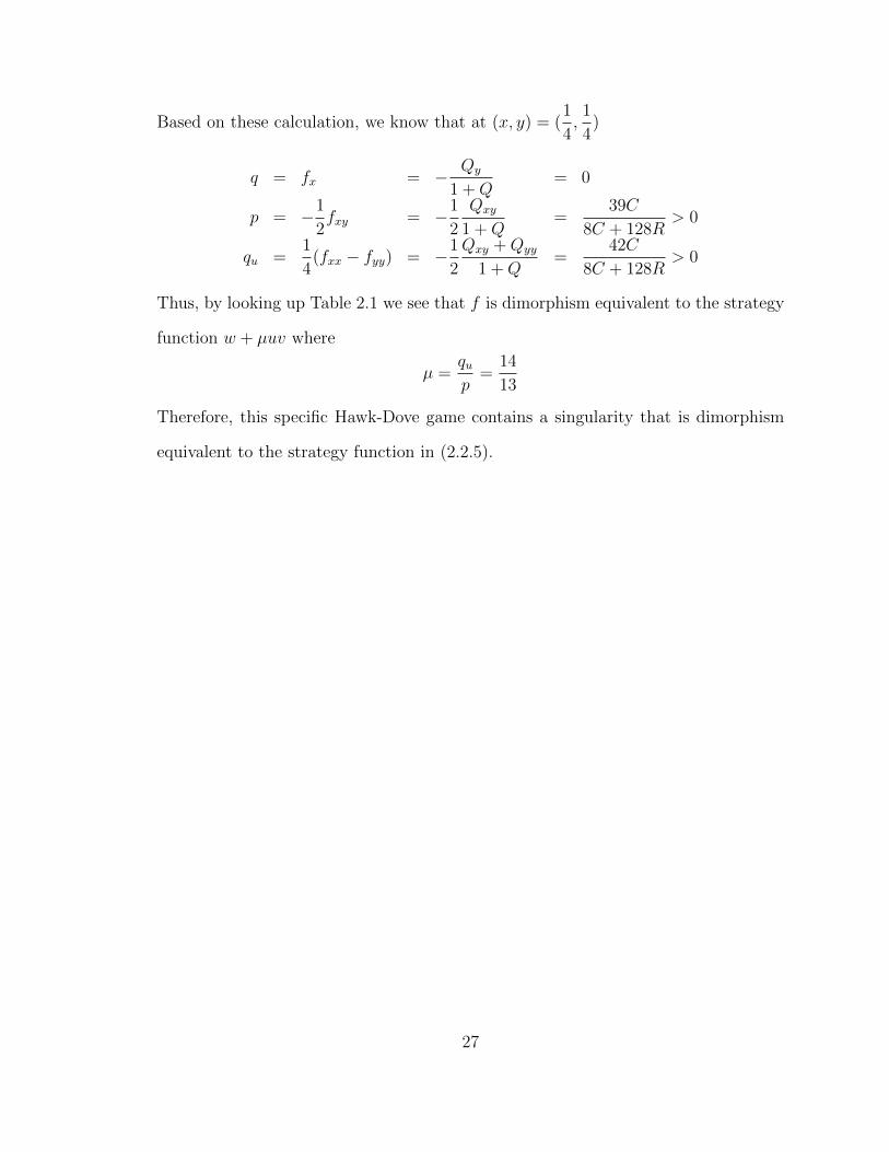
Based on these calculation, we know that at (x, y) = (1

4,1

4)

q = fx = − Qy

1 +Q= 0

p = −1

2fxy = −1

2

Qxy

1 +Q=

39C

8C + 128R> 0

qu =1

4(fxx − fyy) = −1

2

Qxy +Qyy

1 +Q=

42C

8C + 128R> 0

Thus, by looking up Table 2.1 we see that f is dimorphism equivalent to the strategy

function w + µuv where

µ =qup

=14

13

Therefore, this specific Hawk-Dove game contains a singularity that is dimorphism

equivalent to the strategy function in (2.2.5).

27

CHAPTER 3

DIMORPHISM EQUIVALENCE

In this chapter, we review the strategy equivalence (see Definition 3.1) developed by

Golubitsky and Vutha [14]. Strategy equivalence preserves ESS and CvSS singulari-

ties of strategy functions. However, we show in Example 3.2 that strategy equivalence

does not always preserve pairs of dimorphisms. We then introduce a special type of

strategy equivalence that does preserve pairs of dimorphism (Theorem 3.4) and is

called dimorphism equivalence (Definition 3.3). To develop dimorphism equivalence,

we combine strategy equivalence with concepts from singularity theory with symme-

try.

3.1 Strategy Equivalence

Golubitsky and Vutha [14] study strategy functions by defining a form of equivalence

relation that preserves ESS and CvSS singularities. In particular

Definition 3.1. Two strategy functions f and f are strategy equivalent if

f(x, y) = S(x, y)f(Φ(x, y))

where

1. S(x, y) > 0 for all x, y.

2. Φ ≡ (Φ1,Φ2) where Φi: R2 → R, det(dΦ)x,y > 0 for all x, y.

28

3. Φ(x, x) = (φ(x), φ(x)) for every x where φ : R→ R.

4. Φ1,y(x, x) = 0 for every x.

However, this equivalence relation is not strong enough to study dimorphisms in

adaptive dynamics. The following is an example of two strategy functions that are

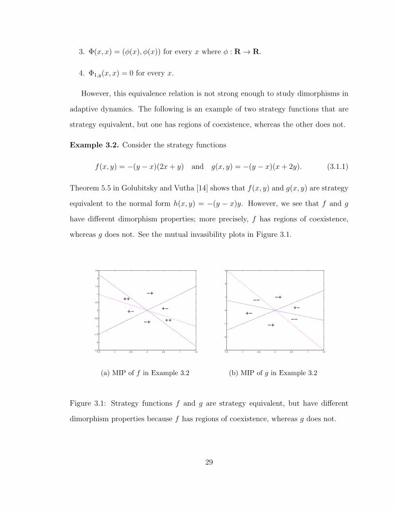
strategy equivalent, but one has regions of coexistence, whereas the other does not.

Example 3.2. Consider the strategy functions

f(x, y) = −(y − x)(2x+ y) and g(x, y) = −(y − x)(x+ 2y). (3.1.1)

Theorem 5.5 in Golubitsky and Vutha [14] shows that f(x, y) and g(x, y) are strategy

equivalent to the normal form h(x, y) = −(y − x)y. However, we see that f and g

have different dimorphism properties; more precisely, f has regions of coexistence,

whereas g does not. See the mutual invasibility plots in Figure 3.1.

−1.5 −1 −0.5 0 0.5 1 1.5

−2.5

−2

−1.5

−1

−0.5

0

0.5

1

1.5

2

2.5

−+

−+

++

++

+−+−

(a) MIP of f in Example 3.2

−1.5 −1 −0.5 0 0.5 1 1.5

−3

−2

−1

0

1

2

3

−+

+−

+−

−−

−+

−−

(b) MIP of g in Example 3.2

Figure 3.1: Strategy functions f and g are strategy equivalent, but have different

dimorphism properties because f has regions of coexistence, whereas g does not.

29

Example 3.2 implies the need for a new equivalence relation to preserve regions

of coexistence. Recall that f(x, y) > 0 indicates a fitness advantage of the mutant

playing strategy y when competing against the resident playing strategy x, whereas

f(y, x) > 0 indicates a fitness advantage of the mutant playing strategy x when

competing against the resident playing the strategy y. We wish to preserve the

regions of coexistence for f under a new equivalence relation, that is, regions where

f(x, y) > 0 and f(y, x) > 0.

Definition 3.3. Two strategy functions f and f are dimorphism equivalent if

f(x, y) = S(x, y)f(Φ(x, y)),

where

1. S(x, y) > 0 for all (x, y).

2. Φ(x, y) = (ϕ(x, y), ϕ(y, x)) where ϕ: R2 → R.

3. (dΦ)x,x = c(x)I2 where c(x) > 0.

Moreover, we call the dimorphism equivalence strong if c(x) ≡ 1.

The remainder of this section is devoted to proving:

Theorem 3.4. If the strategy functions f(x, y) and f(x, y) are dimorphism equiva-

lent, that is,

f(x, y) = S(x, y)f(Φ(x, y)),

where (S,Φ) satisfies the assumptions in Definition 3.3, then the diffeomorphism Φ

maps the regions of coexistence of f(x, y) to those of f(x, y).

Remark 3.5. In fact, we can show that dimorphism equivalence will preserve both

sgn(f(x, y)) and sgn(f(y, x)). There are four regions based on the signs of f(x, y)

and f(y, x) and dimorphism equivalence preserves all of these regions.

30

3.2 Motivation of Dimorphism Equivalence

One way to preserve dimorphisms is to use the same strategy equivalence simultane-

ously on two pairs of strategy functions (f(x, y), f(x, y)) and (f(y, x), f(y, x)). This

idea suggests considering vector functions of the form

F (x, y) =

f(x, y)

f(y, x)

(3.2.1)

where F : R2 → R2 and interpreting dimorphism equivalence as a symmetry condi-

tion on (3.2.1).

Specifically, define the interchange symmetry σ(x, y) = (y, x). Note that every

F (x, y) in (3.2.1) is σ-equivariant, that is

F (σ(x, y)) = σF (x, y). (3.2.2)

In this section we show that specializing σ-equivalence (see [13] for details) to in-

clude the restrictions of strategy equivalence leads to Definition 3.3 of dimorphism

equivalence, and allows us to prove Theorem 3.4. We begin by defining

Definition 3.6. Suppose F (x, y) and F (x, y) are σ-equivariant. Then F (x, y) and

F (x, y) are called modified σ-equivalent if there exists a diffeomorphism Φ : R2 → R2

and a 2× 2 smooth matrix T such that

F (x, y) = T (x, y)F (Φ(x, y)), (3.2.3)

where

T (x, y) =

S(x, y) 0

0 S(y, x)

Φ(x, y) = (ϕ(x, y), ϕ(y, x)) (3.2.4)

and det(T (x, y)) 6= 0, det(dΦ)x,y 6= 0 near the given point.

31

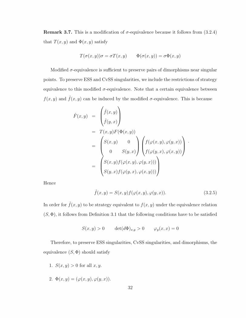
Remark 3.7. This is a modification of σ-equivalence because it follows from (3.2.4)

that T (x, y) and Φ(x, y) satisfy

T (σ(x, y))σ = σT (x, y) Φ(σ(x, y)) = σΦ(x, y)

Modified σ-equivalence is sufficient to preserve pairs of dimorphisms near singular

points. To preserve ESS and CvSS singularities, we include the restrictions of strategy

equivalence to this modified σ-equivalence. Note that a certain equivalence between

f(x, y) and f(x, y) can be induced by the modified σ-equivalence. This is because

F (x, y) =

f(x, y)

f(y, x)

= T (x, y)F (Φ(x, y))

=

S(x, y) 0

0 S(y, x)

f(ϕ(x, y), ϕ(y, x))

f(ϕ(y, x), ϕ(x, y))

=

S(x, y)f(ϕ(x, y), ϕ(y, x)))

S(y, x)f(ϕ(y, x), ϕ(x, y)))

.

Hence

f(x, y) = S(x, y)f(ϕ(x, y), ϕ(y, x)). (3.2.5)

In order for f(x, y) to be strategy equivalent to f(x, y) under the equivalence relation

(S,Φ), it follows from Definition 3.1 that the following conditions have to be satisfied

S(x, y) > 0 det(dΦ)x,y > 0 ϕy(x, x) = 0

Therefore, to preserve ESS singularities, CvSS singularities, and dimorphisms, the

equivalence (S,Φ) should satisfy

1. S(x, y) > 0 for all x, y.

2. Φ(x, y) = (ϕ(x, y), ϕ(y, x)).

32

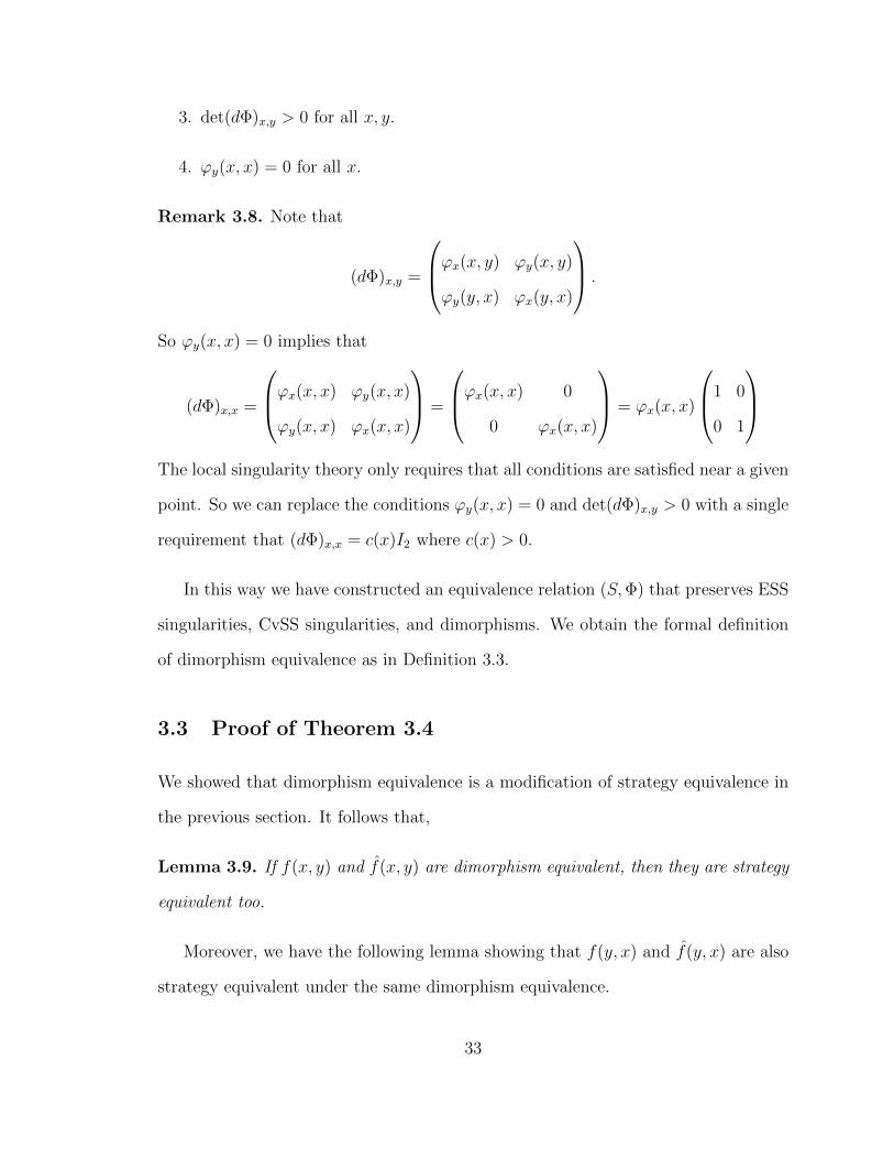
3. det(dΦ)x,y > 0 for all x, y.

4. ϕy(x, x) = 0 for all x.

Remark 3.8. Note that

(dΦ)x,y =

ϕx(x, y) ϕy(x, y)

ϕy(y, x) ϕx(y, x)

.

So ϕy(x, x) = 0 implies that

(dΦ)x,x =

ϕx(x, x) ϕy(x, x)

ϕy(x, x) ϕx(x, x)

=

ϕx(x, x) 0

0 ϕx(x, x)

= ϕx(x, x)

1 0

0 1

The local singularity theory only requires that all conditions are satisfied near a given

point. So we can replace the conditions ϕy(x, x) = 0 and det(dΦ)x,y > 0 with a single

requirement that (dΦ)x,x = c(x)I2 where c(x) > 0.

In this way we have constructed an equivalence relation (S,Φ) that preserves ESS

singularities, CvSS singularities, and dimorphisms. We obtain the formal definition

of dimorphism equivalence as in Definition 3.3.

3.3 Proof of Theorem 3.4

We showed that dimorphism equivalence is a modification of strategy equivalence in

the previous section. It follows that,

Lemma 3.9. If f(x, y) and f(x, y) are dimorphism equivalent, then they are strategy

equivalent too.

Moreover, we have the following lemma showing that f(y, x) and f(y, x) are also

strategy equivalent under the same dimorphism equivalence.

33

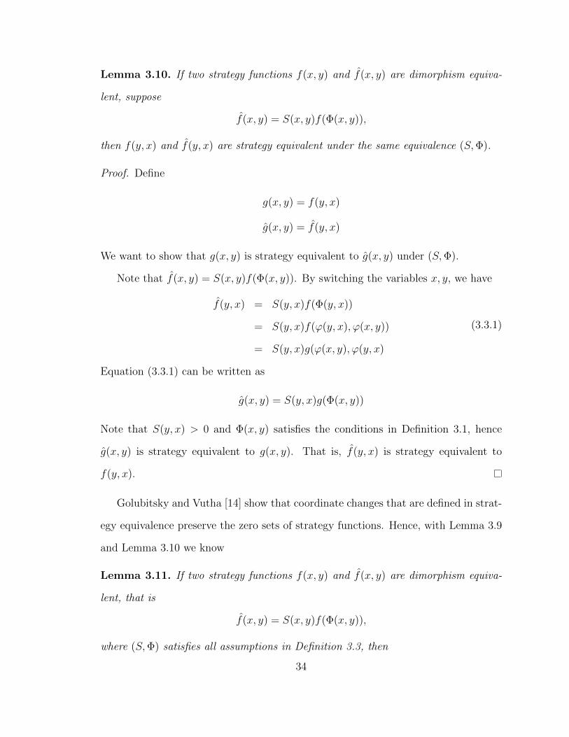
Lemma 3.10. If two strategy functions f(x, y) and f(x, y) are dimorphism equiva-

lent, suppose

f(x, y) = S(x, y)f(Φ(x, y)),

then f(y, x) and f(y, x) are strategy equivalent under the same equivalence (S,Φ).

Proof. Define

g(x, y) = f(y, x)

g(x, y) = f(y, x)

We want to show that g(x, y) is strategy equivalent to g(x, y) under (S,Φ).

Note that f(x, y) = S(x, y)f(Φ(x, y)). By switching the variables x, y, we have

f(y, x) = S(y, x)f(Φ(y, x))

= S(y, x)f(ϕ(y, x), ϕ(x, y))

= S(y, x)g(ϕ(x, y), ϕ(y, x)

(3.3.1)

Equation (3.3.1) can be written as

g(x, y) = S(y, x)g(Φ(x, y))

Note that S(y, x) > 0 and Φ(x, y) satisfies the conditions in Definition 3.1, hence

g(x, y) is strategy equivalent to g(x, y). That is, f(y, x) is strategy equivalent to

f(y, x).

Golubitsky and Vutha [14] show that coordinate changes that are defined in strat-

egy equivalence preserve the zero sets of strategy functions. Hence, with Lemma 3.9

and Lemma 3.10 we know

Lemma 3.11. If two strategy functions f(x, y) and f(x, y) are dimorphism equiva-

lent, that is

f(x, y) = S(x, y)f(Φ(x, y)),

where (S,Φ) satisfies all assumptions in Definition 3.3, then

34

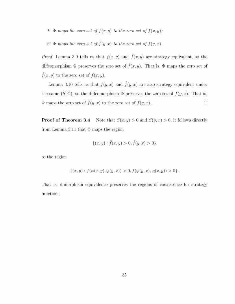
1. Φ maps the zero set of f(x, y) to the zero set of f(x, y);

2. Φ maps the zero set of f(y, x) to the zero set of f(y, x).

Proof. Lemma 3.9 tells us that f(x, y) and f(x, y) are strategy equivalent, so the

diffeomorphism Φ preserves the zero set of f(x, y). That is, Φ maps the zero set of

f(x, y) to the zero set of f(x, y).

Lemma 3.10 tells us that f(y, x) and f(y, x) are also strategy equivalent under

the same (S,Φ), so the diffeomorphism Φ preserves the zero set of f(y, x). That is,

Φ maps the zero set of f(y, x) to the zero set of f(y, x).

Proof of Theorem 3.4 Note that S(x, y) > 0 and S(y, x) > 0, it follows directly

from Lemma 3.11 that Φ maps the region

{(x, y) : f(x, y) > 0, f(y, x) > 0}

to the region

{(x, y) : f(ϕ(x, y), ϕ(y, x)) > 0, f(ϕ(y, x), ϕ(x, y)) > 0}.

That is, dimorphism equivalence preserves the regions of coexistence for strategy

functions.

35

CHAPTER 4

THE RESTRICTED TANGENT SPACE

In this chapter, we answer the question: when is f+η dimorphism equivalent to f for

a small perturbation η? WLOG, we assume that f and η are both strategy functions

and (0, 0) is the singularity for both of them.

First, by applying singularity theory, we reduce the question that is set in an

infinite dimensional functional space to a question that is set in a finite dimensional

polynomial ring. To do so, we introduce the dimorphism equivalence restricted tangent

space: the subspace of all strategy function perturbations η that satisfies f + tη is

dimorphism equivalent to f for all small t. We find the general form for the strategy

function η in Proposition 4.2. By applying the form of η we prove the tangent space

constant theorem (see Theorem 4.7) in the context of dimorphism equivalence.

We find that the calculations are more easily done in the coordinate system

u = x+ y

v = x− y(4.0.1)

and we set w = v2.

36

4.1 A Change of Coordinates

The idea of considering σ-symmetry (where σ(x, y) = (y, x)) when studying dimor-

phisms motivates the coordinate change in Lemma 4.1. Note that under (u, v) coor-

dinates in (4.0.1), we have σ(u, v) = (u,−v).

Lemma 4.1. Every smooth real-valued function a(u, v) can be written in the form

a(u, v) = b(u,w) + c(u,w)v (4.1.1)

where b and c are smooth functions.

Proof. For the proof see the discussion in [11, p.108]. It follows that every smooth

real-valued function a can be written as a pair of smooth σ-invariant functions b, c as

in (4.1.1).

Let f be a strategy function. Since f(x, x) = 0 or in (u, v) coordinates f(u, 0) = 0,

it follows from Lemma 4.1 that f can be defined as

f = b(u,w) + q(u,w)v

where b(u, 0) = 0. By Taylor’s Theorem f has the form

f = p(u,w)w + q(u,w)v,

where p, q : R2 → R are smooth functions. In the remainder of this thesis we will

identify strategy functions f with the notation [p, q] ∈ E2 where E is the space of

smooth real-valued functions in (u,w) coordinates.

4.2 Dimorphism Equivalence Restricted Tangent Space

Assume that f + tη is dimorphism equivalent to f for all small t. That is, suppose

there exists a smooth t-dependent dimorphism equivalence such that

f(x, y) + tη(x, y) = S(x, y, t)f(Φ(x, y, t)) (4.2.1)

37

where

S(x, y, 0) = 1 ϕ(x, y, 0) = x ϕ(0, 0, t) = 0 S(x, y, t) > 0

Φ(x, y, t) = (ϕ(x, y, t), ϕ(y, x, t)) ϕy(x, x, t) = 0 ϕx(x, x, t) > 0(4.2.2)

Differentiating both sides of (4.2.1) with respect to t and evaluating at t = 0 gives

η(x, y) = S(x, y, 0)f(x, y) + ϕ(x, y, 0)fx(x, y) + ϕ(y, x, 0)fy(x, y) (4.2.3)

where · is the derivative with respect to t and (S,Φ) satisfies all the requirements in

(4.2.2).

We define the dimorphism equivalence restricted tangent space RT (f) of f to be

the space of all η(x, y) that satisfies (4.2.3) where (S,Φ) satisfies all assumptions in

(4.2.2).

Proposition 4.2. Let f = pw + qv, the dimorphism equivalence restricted tangent

space RT (f) is

〈[p, q], [q, wp], [wpu, wqu], [wp+ 2w2pw, 2w2qw]〉+ R{. . .}

where {· · · } indicates the R–module generated by

uj−1[jp+ upu + 2jwpw, uqu + 2jwqw]

for j = 1, 2, . . ..

Proof. Dimorphism equivalences are generated by two kinds of equivalence

1. f(x, y) = S(x, y)f(x, y) where S(x, y) > 0.

2. f(x, y) = f(ϕ(x, y), ϕ(y, x)) where ϕ(0, 0) = 0, ϕy(x, x) = 0, ϕx(x, x) > 0.

Consider the first type of equivalences in (u, v) coordinates, we can assume that

S = Se(u,w) + So(u,w)v

38

where Se(0, 0) > 0. Then the tangent vectors given by this type of equivalencies can

be computed by

d

dtS(x, y, t)f(x, y)

∣∣∣∣t=0

= S(x, y, 0)f(x, y)

= (Se + Sov)(pw + qv)

= Se(pw + qv) + So(qw + wpv)

where · is the derivative with respect to t. Since Se and So are arbitrary σ-invariant

functions we see that

〈[p, q], [q, wp]〉 ⊂ RT (f)

Consider the second type of equivalences in (u, v) coordinates, we can assume

ϕ(x, y, t) = ϕe(u,w, t) + ϕo(u,w, t)v.

Since ϕ(y, x, t) = ϕe(u,w, t)− ϕo(u,w, t)v, we compute

u(Φ(x, y, t)) = ϕ(x, y, t) + ϕ(y, x, t) = (ϕe + ϕov) + (ϕe − ϕov) = 2ϕe

v(Φ(x, y, t)) = ϕ(x, y, t)− ϕ(y, x, t) = (ϕe + ϕov)− (ϕe − ϕov) = 2ϕov

w(Φ(x, y, t) = v(Φ(x, y, t))2 = (2ϕov)2 = 4ϕ2ow

(4.2.4)

Then the tangent vectors given by this type of equivalencies can be computed by

d

dtf(ϕ(x, y, t), ϕ(y, x, t))

∣∣∣∣t=0

(4.2.5)

Using (4.2.4) we calculate the derivative in (4.2.5) as

d

dtf(ϕ(x, y, t), ϕ(y, x, t))

=d

dt(p(u(Φ), v(Φ)2)v(Φ)2 + q(u(Φ), v(Φ)2)v(Φ))

=d

dt(4p(2ϕe, 4ϕ

2ow)ϕ2

ow + 2q(2ϕe, 4ϕ2ow)ϕov)

= 8p1ϕ2owϕe + 32p2w

2ϕ3oϕo + 8pwϕoϕo + 4q1ϕovϕe + 16q2wvϕ

2oϕo + 2qvϕo

= ϕe(8p1ϕ2ow + 4q1ϕov) + ϕo(32p2w

2ϕ3o + 8pwϕo + 16q2wvϕ

2o + 2qv)

39

where pi, qi are the derivative of p, q respect to the ith component (i = 1, 2) and · is

the derivative with respect to t.

Note that the diffeomorphism Φ is the identity at t = 0, we have

x = ϕ(x, y, 0) = ϕe(u,w, 0) + ϕo(u,w, 0)v

Then we have

ϕe(u,w, 0) =1

2u ϕo(u,w, 0) =

1

2(4.2.6)

Using (4.2.6) and evaluating at t = 0, we obtain

d

dtf(ϕ(x, y, t), ϕ(y, x, t))

∣∣∣∣t=0

= 2ϕe(puw+quv)+4ϕo(pww2+pw+qwwv+

1

2qv) (4.2.7)

Note that

ϕy(x, x, t) = (ϕe)u(2x, 0, t)− ϕo(2x, 0, t)

It follows from ϕy(x, x, t) = 0 that

ϕo(u, 0, t) = (ϕe)u(u, 0, t)

Hence, we can write

ϕe(u,w, t) =1

2u+ g(u,w, t)t ϕo(u,w, t) =

1

2+ h(u,w, t)t.

Therefore

(ϕe)u(u, 0, t) =1

2+ gu(u, 0, t)t ϕo(u, 0, t) =

1

2+ h(u, 0, t)t.

Then we have

gu(u, 0, t) = h(u, 0, t)

In addition,

ϕe =d

dtϕe(u,w, t)|t=0 = g(u,w, 0) = g(u, 0, 0) + g(u,w, 0)w

40

ϕo =d

dtϕo(u,w, t)|t=0 = h(u,w, 0) = h(u, 0, 0) + h(u,w, 0)w

where h(u, 0, 0) = gu(u, 0, 0) and g, h are arbitrary.

Now we redefine the functions g, g, h such that g : R → R, g, h : R2 → R. It

follows that the RHS of (4.2.7) contains

2(g(u) + wg(u,w))(puw + quv) + 4(g′(u) + wh(u, v))(pww2 + pw + qwwv +

1

2qv)

In [· · · , · · · ] notation, we have

2g[puw, quw] + 2h[2pw + 2pww2, qw + 2qww

2]

+ 2g(u)(puw + quv) + 2g′(u)(2pww2 + 2pw + 2qwwv + qv)

Since g(u,w), h(u,w), g(u) are arbitrary σ invariant functions, we see that

〈[puw, quw], [2pw + 2pww2, qw + 2qww

2]〉 ⊂ RT (f)

Moreover, the dimorphism equivalence restricted tangent space includes the vectors

2g(u)(puw + quv) + 2g′(u)(2pww2 + 2pw + 2qwwv + qv)

for arbitrary g(u). Therefore, now we have

〈[p, q], [q, wp], [wpu, wqu], [2wp+ 2w2pw, qw + 2w2qw]〉 ⊂ RT (f)

Note that we can simplify 〈[p, q], [2pw + 2pww2, qw + 2qww

2]〉 into

〈[p, q], [pw + 2pww2, 2qww

2]〉

Therefore, we have proved the ideal part of expression of RT (f) as follows

〈[p, q], [q, wp], [wpu, wqu], [wp+ 2w2pw, 2w2qw]〉 ⊂ RT (f)

Next we continue to find the vector part of RT (f). Note that in the definition of

RT (f), we require that ϕ(0, 0, t) = 0 for all small t. Then we have

∂ϕ

∂t(0, 0, 0) = ϕe(0, 0, 0) = g(0) = 0.

41

Therefore, g satisfies the following

g(u) = k1u+ k2u2 + · · ·+ kju

j + · · ·

g′(u) = k1 + 2k2u+ · · ·+ jkjuj−1 + · · ·

It follows that (g(u), g′(u)) can be any element in the vector space spanned by

(u, 1) (u2, 2u) (u3, 3u) · · ·

It follows from (4.2.7) that the dimorphism equivalence restricted tangent space in-

cludes the vectors

uj(puw + quv) + juj−1(2pww2 + 2pw + 2qwwv + qv)

where j = 1, 2, . . .. Hence the {· · · } notation in the statements of Proposition 4.2 is

uj−1[jp+ upu + 2jwpw, uqu + 2jwqw]

for j = 1, 2, . . ..

Remark 4.3. Note that in Definition 3.3, we define the strongly dimorphism equiv-

alence. If we try to calculate the restricted tangent space of a strategy functions f in

the context of strongly dimorphism equivalence, we would go through similar calcu-

lations except that we will not have the vector terms in {· · · }. That is, the strongly

dimorphism equivalence restricted tangent space of a strategy function f = pw + qv

is

〈[p, q], [q, wp], [wpu, wqu], [wp+ 2w2pw, 2w2qw]〉

Remark 4.4. In the definition of RT (f), we require that ϕ(0, 0, t) = 0, that is, the

singularity is always at (0, 0). However, a general perturbation of a strategy function

f does not always have this restriction. If this condition does not hold, we have the

definition of dimorphism equivalence tangent space, denoted by T (f): the space of

42

η(x, y) that satisfies (4.2.1) where (S,Φ) satisfies all assumptions in (4.2.2) except

the one ϕ(0, 0, t) = 0. To calculate the dimorphism equivalence tangent space T (f),

we eliminate the restriction g(0) = 0. It lead to an additional vector R{[pu, qu]} . We

will discuss this in detail in Chapter 6.

With Proposition 4.2 we can compute the dimorphism equivalence restricted tan-

gent space of a strategy function. Define

I(f) = 〈[p, q], [q, wp], [wpu, wqu], [wp+ 2w2pw, 2w2qw]〉 (4.2.8)

Remark 4.5. In the proof of Proposition 4.2, we showed that there is an alternative

expression for I(f) as below

I(f) = 〈[p, q], [q, wp], [wpu, wqu], [2pw + 2pww2, qw + 2qww

2]〉 (4.2.9)

Remark 4.6. Note that Remark 4.3 shows that I(f) is in fact the restricted tangent

space of f in the context of strongly dimorphism equivalence.

Recall that a strategy s is a singular strategy if fy(s, s) = 0. Under the (u, v)

coordinates, since we assume that f(x, y) = p(u,w)w+ q(u,w)v, we call a strategy s

a singular strategy if q(2s, 0) = 0.

4.3 Modified Tangent Space Constant Theorem

The definition of RT (f) implies that if f + tη is dimorphism equivalent to f for all

small t, then η ∈ RT (f). In the converse direction, we have Theorem 4.7.

Theorem 4.7 (Modified Tangent Space Constant Theorem). Let f be a strategy

function. If

I(f + tg) = I(f) for all t ∈ [0, 1] (4.3.1)

Then f + tg is strongly dimorphism equivalent to f for all t ∈ [0, 1].

43

Remark 4.8. The proof of this theorem is a modification of the proof of an analogous

theorem in bifurcation theory (see [12] Theorem 2.2).

Proof. In this proof, we use the alternative form of I(f) as in (4.2.9). Suppose

I(f + t0g) = I(f) for some t0 6= 0 and f = pfw + qfv, g = pgw + qgv. Let

F (x, y, t) = f(x, y) + tg(x, y) (4.3.2)

We prove the statement in following steps. We show in order

(a) There exist smooth functions A(u,w, t), B(u,w, t), C(u,w, t) and D(u,w, t)

such that

g = [pg, qg]

= A[pF , qF ] +B[qF , wpF ] + C[wpFu , wqFu ]

+D[2wpF + 2w2pFw, wqF + 2w2qFw ]

(4.3.3)

(b) F (x, y, t) is strongly dimorphism equivalent to f(x, y) for each t sufficiently

close to 0.

(c) F (x, y, t) is strongly dimorphism equivalent to f(x, y) for all t ∈ [0, 1].

We show (a). Note that for each fixed t, I(f + tg) = I(f) implies that there exist

functions A, B, C, D such that (4.3.3) holds. In (a), we imply that A, B, C, D can

be chosen to vary smoothly in t.

Choose t0 near 0 so that

I(f + t0g) = I(f)

In particular, each generator of I(f + t0g) can be written as a linear combination

44

of generators of I(f). Therefore, there exist functions Ai(u,w), Bi(u,w), Ci(u,w),

Di(u,w)for 1 ≤ i ≤ 4 such that

[pf + t0pg, qf + t0q

g] = A1[pf , qf ] +B1[qf , wpf ] + C1[wpfu, wqfu]

+D1[2wpf + 2w2pfw, wqf + 2w2qfw]

[qf + t0qg, w(pf + t0p

g)] = A2[pf , qf ] +B2[qf , wpf ] + C2[wpfu, wqfu]

+D2[2wpf + 2w2pfw, wqf + 2w2qfw]

[w(pfu + t0pgu), w(qfu + t0q

gu)] = A3[pf , qf ] +B3[qf , wpf ] + C3[wpfu, wq

fu]

+D3[2wpf + 2w2pfw, wqf + 2w2qfw]

[2w(pf + t0pg) + 2w2(pfw + t0p

gw), = A4[pf , qf ] +B4[qf , wpf ] + C4[wpfu, wq

fu]

w(qf + t0qg) + 2w2(qfw + t0q

gw)] +D4[2wpf + 2w2pfw, wq

f + 2w2qfw]

(4.3.4)

Rearranging terms in (4.3.4), we obtain a matrix equation

[pg, qg]

[qg, wpg]

[wpgu, wqgu]

[2wpg + 2w2pgw, wqg + 2w2qgw]

= Q

[pf , qf ]

[qf , wpf ]

[wpfu, wqfu]

[2wpf + 2w2pfw, wqf + 2w2qfw]

(4.3.5)

where

Q =1

t0

A1 − 1 B1 C1 D1

A1 B1 − 1 C1 D1

A1 B1 C1 − 1 D1

A1 B1 C1 D1 − 1

is a 4× 4 matrix whose entries are smooth functions.

Next, for any strategy function h, let

z(h) =

[ph, qh]

[qh, wph]

[wphu, wqhu]

[2wph + 2w2phw, wqh + 2w2qhw]

45

Using this notation, rewrite (4.3.5) as

z(g) = Qz(f) (4.3.6)

By (4.3.2), f = F − tg. Therefore,

z(f) = z(F )− tz(g) (4.3.7)

Substituting (4.3.7) into (4.3.6) and rearranging, we find

(I + tQ)z(g) = Qz(F ) (4.3.8)

Observe that (4.3.8) is a system of four equations with smooth dependence on t. Since

I is invertible, I + tQ is also an invertible 4× 4 matrix for small t. Thus (I + tQ)−1

is a 4× 4 matrix whose entries are smooth functions in t. The invertibility of I + tQ

and (4.3.8) imply

z(g) = (I + tQ)−1Qz(F ) (4.3.9)

(a) follows from equating the first components on each side of the matrix equation

(4.3.9).

We show (b). Specifically, we construct a strongly dimorphism equivalence map-

ping (S(x, y, t),Φ(x, y, t)) varying smoothly in t and satisfying that

S(x, y, t)F (Φ(x, y, t), t) = f(x, y)

S(x, y, 0) = 1

Φ(x, y, 0) = (x, y)

ϕx(x, x, t) = 1

ϕy(x, x, t) = 0

(4.3.10)

The functions Φ and S are found by solving certain ODE’s. From direct calculation

in Proposition 4.2, we can write (S,Φ) in the following form

S(x, y, t) = Se(u,w, t) + So(u,w, t)v

ϕ(x, y, t) = ϕe(u,w, t) + ϕo(u,w, t)v

46

Now, we consider the following two sets of system of differential equations

ϕe(u,w, t) = −2ϕ2owC(2ϕe, 4ϕ

2ow)

ϕo(u,w, t) = −4ϕ3owD(2ϕe, 4ϕ

2ow)

ϕe(u,w, 0) =1

2u

ϕo(u,w, 0) =1

2

(4.3.11)

and

Se(u,w, t) = −(SeA(2ϕe, 4ϕ2ow) + SoB(2ϕe, 4ϕ

2ow)2ϕow)

So(u,w, t) = −(SoA(2ϕe, 4ϕ2ow) + S0B(2ϕe, 4ϕ

2ow))

Se(u,w, 0) = 1

So(u,w, 0) = 0

(4.3.12)

where A,B,C,D are the coefficients in (4.3.3).

Suppose there exists solutions (ϕe, ϕo, Se, So) of the ODEs (4.3.11) and (4.3.12)

on a neighborhood of K × L×M ×N and denote

[p, q]Φ = p(Φ)w(Φ) + q(Φ)v(Φ)

47

Then we have

d

dt(S(x, y, t)F (Φ, t))

=d

dt((Se + Sov)(pF (Φ)w(Φ) + qF (Φ)v(Φ)))

=d

dt[(Se + Sov)](pF (Φ)w(Φ)

+qF (Φ)v(Φ)) + (Se + Sov)d

dt[(pF (Φ)w(Φ) + qF (Φ)v(Φ))]

= (Se + Sov)(pF (Φ)w(Φ) + qF (Φ)v(Φ))

+(Se + Sov)d

dt(pF (2ϕe, 4ϕ

2o, t)4ϕ

2ow + qF (2ϕe, 4ϕ

2o, t)2ϕov)

= Se[pF , qF ]Φ + Sov[pF , qF ]Φ + (Se + Sov)[(pFu (2ϕe, 4ϕ

2o, t)(2ϕe)4ϕ

2o

+pFw(2ϕe, 4ϕ2o, t)(8ϕoϕo)4ϕ

2o + pF (2ϕe, 4ϕ

2o, t)8ϕoϕo + pFt (2ϕe, 4ϕ

2o, t)4ϕ

2o)w

+(qFu (2ϕe, 4ϕ2o, t)(2ϕe)2ϕo + qFw (2ϕe, 4ϕ

2o, t)(8ϕoϕo)2ϕo

+qF (2ϕe, 4ϕ2o, t)2ϕo + qFt (2ϕe, 4ϕ

2o, t)2ϕo)v]

= Se[pF , qF ]Φ +

So2ϕo

[qF , wpF ]Φ + (Se + Sov)(ϕe

2ϕ2ow

[wpFu , wqFu ]Φ

+ϕo

4ϕ3ow

[2wpF + 2w2pFw, wqF + 2w2qFw ]Φ + [pFt , q

Ft ]Φ)

(4.3.13)

Note that in part (a), we have

g = [pg, qg] = A[pF , qF ]+B[qF , wpF ]+C[wpFu , wqFu ]+D[2wpF +2w2pFw, wq

F +2w2qFw ].

48

Therefore,

(Se + Sov)g(Φ)

= (Se + Sov)[pg, qg]Φ

= (Se + Sov)(A(Φ)[pF , qF ]Φ +B(Φ)[qF , wpF ]Φ+

C(Φ)[wpFu , wqFu ]Φ +D(Φ)[wpF + 2w2pFw, 2w

2qFw ]Φ)

= (Se + Sov)A(Φ)[pF , qF ]Φ + (Se + Sov)B(Φ)[qF , wpF ]Φ

+(Se + Sov)(C(Φ)[wpFu , wqFu ]Φ +D(Φ)[wpF + 2w2pFw, 2w

2qFw ]Φ)

= SeA(Φ)[pF , qF ]Φ + SoA(Φ)[qF , wpF ]Φ + S0B(Φ)[qF , wpF ]Φ + SoB(Φ)2ϕow[pF , qF ]Φ

+(Se + Sov)(C(Φ)[wpFu , wqFu ]Φ +D(Φ)[wpF + 2w2pFw, 2w

2qFw ]Φ)

= (SeA(Φ) + SoB(Φ)2ϕow)[pF , qF ]Φ + (SoA(Φ) + S0B(Φ))[qF , wpF ]Φ

+(Se + Sov)C(Φ)[wpFu , wqFu ]Φ + (Se + Sov)D(Φ)[wpF + 2w2pFw, 2w

2qFw ]Φ

The right-hand side of (4.3.13) can be simplified considering the fact that (ϕe, ϕo, S0, S1)

are the solutions to the ODEs (4.3.11) and (4.3.12). Then we have

d

dt(S(x, y, t)F (Φ, t))

= Se[pF , qF ]Φ +

So2ϕo

[qF , wpF ]Φ

+(Se + Sov)(ϕe

2ϕ2ow

[wpFu , wqFu ]Φ +

ϕo4ϕ3

ow[2wpF + 2w2pFw, 2w

2qFw ]Φ + [pFt , qFt ]Φ)

= −(SeA(Φ) + SoB(Φ)2ϕow)[pF , qF ]Φ − (SoA(Φ) + S0B(Φ))[qF , wpF ]Φ

+(Se + Sov)(−C(Φ)[wpFu , wqFu ]Φ −D(Φ)[2wpF + 2w2pFw, 2w

2qFw ]Φ + [pg, qg]Φ)

= 0

Hence,

S(x, y, t)F (Φ(x, y, t), t) = S(x, y, 0)F (Φ(x, y, 0), t) = f(x, y)

In other words, F (x, y, t) = f(x, y) + tg(x, y) is strongly dimorphism equivalent to

f(x, y) when t is small enough around 0.

Now we show that (ϕe, ϕo, S0, S1) can be chosen to satisfy all conditions in (4.3.10).

49

Note that all conditions are explicitly expressed in the ODEs (4.3.11) and (4.3.12)

except ϕx(x, x, t) = 1 and ϕy(x, x, t) = 0. In Proposition 4.2, we showed that

ϕy(x, x, t) = (ϕe)u(2x, 0, t)− ϕo(2x, 0, t)

Therefore with ODEs (4.3.11) we have

d

dt(ϕx(x, x, t)) =

d

dt((ϕe)u(2x, 0, t) + ϕo(2x, 0, t))

= (ϕe)u(2x, 0, t) + ϕo(2x, 0, t) = 0 + 0 = 0

d

dt(ϕy(x, x, t)) =

d

dt((ϕe)u(2x, 0, t)− ϕo(2x, 0, t))

= (ϕe)u(2x, 0, t)− ϕo(2x, 0, t) = 0− 0 = 0

Hence

ϕx(x, x, t) = (ϕe)u(2x, 0, t) + ϕo(2x, 0, t)

= (ϕe)u(2x, 0, 0) + ϕo(2x, 0, 0)

=1

2+

1

2= 1

ϕy(x, x, t) = (ϕe)uu(2x, 0, t)− ϕo(2x, 0, t)

= (ϕe)u(2x, 0, 0)− ϕo(2x, 0, 0)

=1

2− 1

2= 0

This means that the solution (ϕe, ϕo, S0, S1) are the solutions to the ODEs (4.3.11)

and (4.3.12) and satisfy all the conditions in (4.3.10).

The standard existence theorem for ODEs with smooth dependence on parameters

implies that there exists intervals K×L×M×N where the ODEs (4.3.11) and (4.3.12)

have unique solutions. Therefore, (b) holds.

We show (c). Define t1 and t2 in [0, 1] to be equivalent if f + t1g is strongly

50

dimorphism equivalent to f + t2g. We claim that (b) implies equivalence classes of

t’s in [0, 1] are open. To verify this, assume h = f + t0g for some t0 ∈ [0, 1]. Then,

I(h+ sg) = I(f + (s+ t0)g) = I(f) = I(h)

for all s sufficiently near 0. By part (b), h+ sg is strongly dimorphism equivalent to

h for all s near 0. Thus f + t0g is strongly dimorphism equivalent to f + tg for all t

near t0 and the equivalence class for t’s are open.

It follows from compactness of [0, 1] that there is exactly one equivalence class.

Hence, part (c) holds and f + tg is strongly dimorphism equivalent to f for all

t ∈ [0, 1].

51

CHAPTER 5

RECOGNITION OF LOW CODIMENSION

SINGULARITIES

This chapter is devoted to proving Theorem 5.1. Note that strategy functions f have

singularities at (0, 0) and all derivatives of f are computed at (0, 0) unless otherwise

indicated.

Theorem 5.1. Suppose f = p(u,w)w + q(u,w)v is a strategy function with a singu-

larity at the origin. Then f is dimorphism equivalent to the normal form in Table 5.1

if and only if the corresponding defining conditions and non-degeneracy conditions in

Table 5.1 are satisfied.

In this theorem, we apply the modified tangent space constant theorem (The-

orem 4.7) to solve the recognition problem for low codimension singularities under

dimorphism equivalence. To prove this theorem, we use Nakayama’s Lemma (cf. [12,

Chapter 2]), which we now state.

Remark 5.2. In this thesis E is the ring of functions z(u,w) (defined on a neighbor-

hood of the origin) and M is the maximal ideal in E generated by u,w.

Lemma 5.3. [Nakayama’s Lemma]. Let I, J ⊂ E2 be a finitely generated E-modules.

Then

I ⊂ J if and only if I ⊂ J +MI

52

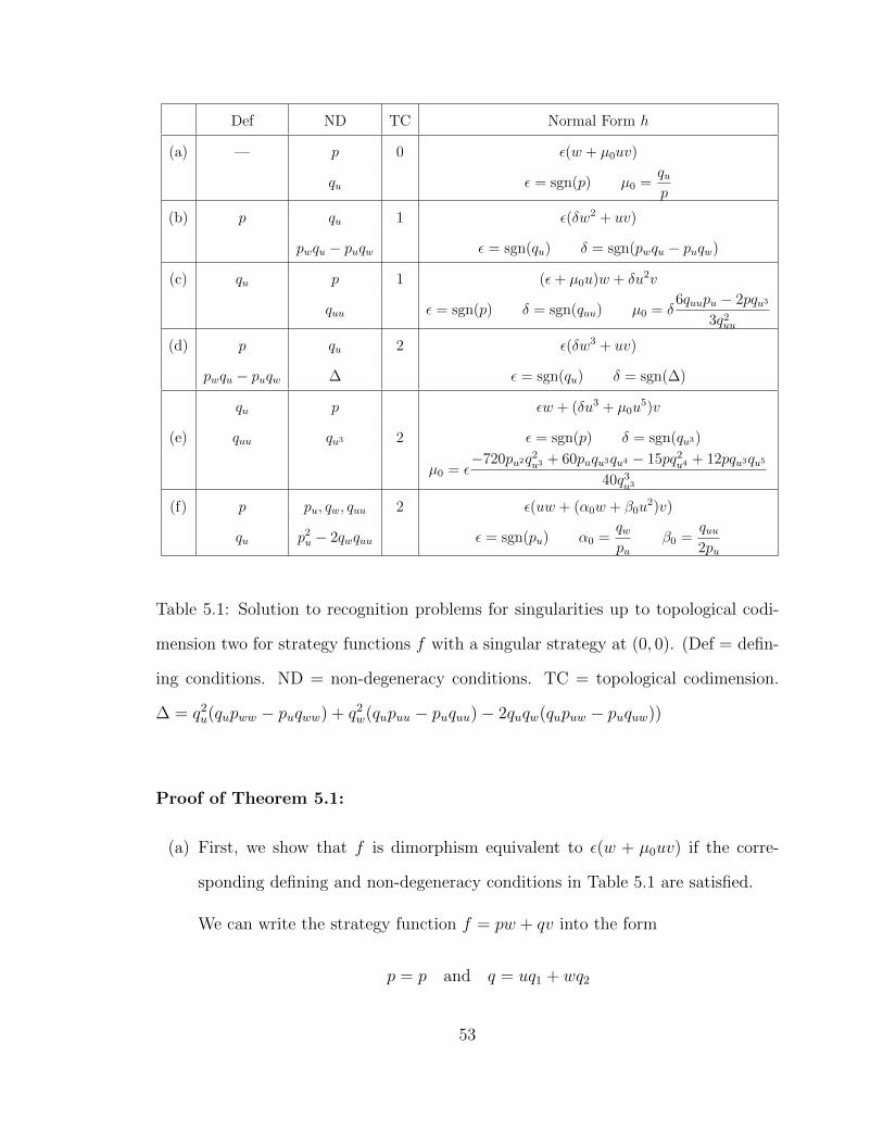
Def ND TC Normal Form h

(a) — p 0 ε(w + µ0uv)

qu ε = sgn(p) µ0 =qup

(b) p qu 1 ε(δw2 + uv)

pwqu − puqw ε = sgn(qu) δ = sgn(pwqu − puqw)

(c) qu p 1 (ε+ µ0u)w + δu2v

quu ε = sgn(p) δ = sgn(quu) µ0 = δ6quupu − 2pqu3

3q2uu

(d) p qu 2 ε(δw3 + uv)

pwqu − puqw ∆ ε = sgn(qu) δ = sgn(∆)

qu p εw + (δu3 + µ0u5)v

(e) quu qu3 2 ε = sgn(p) δ = sgn(qu3)

µ0 = ε−720pu2q

2u3 + 60puqu3qu4 − 15pq2

u4 + 12pqu3qu5

40q3u3

(f) p pu, qw, quu 2 ε(uw + (α0w + β0u2)v)

qu p2u − 2qwquu ε = sgn(pu) α0 =

qwpu

β0 =quu2pu

Table 5.1: Solution to recognition problems for singularities up to topological codi-

mension two for strategy functions f with a singular strategy at (0, 0). (Def = defin-

ing conditions. ND = non-degeneracy conditions. TC = topological codimension.

∆ = q2u(qupww − puqww) + q2

w(qupuu − puquu)− 2quqw(qupuw − puquw))

Proof of Theorem 5.1:

(a) First, we show that f is dimorphism equivalent to ε(w + µ0uv) if the corre-

sponding defining and non-degeneracy conditions in Table 5.1 are satisfied.

We can write the strategy function f = pw + qv into the form

p = p and q = uq1 + wq2

53

where p(0, 0) 6= 0 and q1(0, 0) 6= 0. We calculate I(f). With formula (4.2.8),

we have

[p, q] = [p, uq1 + wq2]

[q, wp] = [uq1 + wq2, wp]

[wpu, wqu] = [wpu, w(q1 + u(q1)u + w(q2)u)]

[wp+ 2w2pw, 2w2qw] = [wp+ 2w2pw, 2w

2(u(q1)w + q2 + w(q2)w)]

We claim that [M,M2] ⊂ I(f). With Nakayama’s Lemma, we need to prove

[M,M2] ⊂ I(f) + [M2,M3]

Let J = I(f) + [M2,M3]. We have

M[uq1 + wq2, wp] ∈ J ⇒ [0, wM] ∈ J

[0, wM], w[p, uq1 + wq2] ∈ J ⇒ [w, 0] ∈ J

[w, 0], [0, wM], [wpu, w(q1 + u(q1)u + w(q2)u)] ∈ J ⇒ [0, w] ∈ J

[w, 0], [0, w], [uq1 + wq2, wp] ∈ J ⇒ [u, 0] ∈ J

[u, 0], [0, wM], u[p, uq1 + wq2] ∈ J ⇒ [0, u2] ∈ J

Thus we have proved the claim that [M,M2] ⊂ I(f). Therefore, J = I. The

above calculation shows that

〈[w, 0], [u, 0], [0, w], [0, u2]〉 ⊂ I(f).

Denote

K = 〈[w, 0], [u, 0], [0, w], [0, u2]〉

We know that

I(f) = K + 〈[p(0, 0), uq1(0, 0)]〉

Since for any strategy function h inside the module K, f + th satisfies all the

defining and non-degeneracy conditions of the theorem. Thus we know that

I(f + th) = I(f)

54

for all h ∈ K, t ∈ [0, 1]. According to Theorem 4.7, we know that f + h is

dimorphism equivalent to f . So we can assume that f is in the following form:

f = p00w + q10uv

where

p00 = p(0, 0) 6= 0 q10 = qu(0, 0) 6= 0

Next, we will try to further simplify the form of the strategy function f with

specific dimorphism equivalence transformation.

As discussed earlier, for any h ∈ K we have

I(f) = I(f + h)

Thus in the following calculation, we can modulo K, that is, we will ignore all

terms in K during the dimorphism transformation.

Let (S,Φ) satisfy that

S = Se + Sov Φ = (ϕe + ϕov, ϕe − ϕov)

where Se, So, ϕo, ϕe ∈ E . In Proposition 4.2, we show

u(Φ) = 2ϕe v(Φ) = 2ϕov w(Φ) = 4ϕ2ow

ϕe(0, 0) = 0 (ϕe)u(u, 0) = ϕo(u, 0)

Now consider the case when

Se =ε

p00

So = 0

ϕe =1

2u

ϕo =1

2

55

By the definition of dimorphism equivalence, we know f is dimorphism equiv-

alent to g = Sf(Φ). That is,

g = (Se + Sov)(p(Φ)w(Φ) + q(Φ)v(Φ))

= (Sep(Φ)w(Φ) + Soq(Φ)v(Φ)v) + (Seq(Φ)v(Φ) + Sop(Φ)w(Φ)v)

= (Sep(Φ)(4ϕ2o) + Soq(Φ)(2ϕo))w + (Seq(Φ)(2ϕo) + Sop(Φ)(4ϕ2

o)w)v

= (ε+ ph(u,w))w + (εq10

p00

u+ qh(u,w))v

where [ph, qh] ∈ K. Therefore, we have shown that f is dimorphism equivalent

to

ε(w + µ0uv)

where at (0, 0)

ε = sgn(p) µ0 =qup

At the end, we prove that if f = pw + qv is dimorphism equivalent to

h = ε(w + µ0uv)

where µ0 6= 0 and the singularity is at (0, 0), then the corresponding defining

and non-degeneracy conditions in Table 5.1 hold. The dimorphism equivalence

indicates that there exists a dimorphism equivalence transformation (S,Φ) such

that f = Sh(Φ) and we can write

S = Se + Sov Φ = (ϕe + ϕov, ϕe − ϕov)

where at (0, 0)

Se > 0 ϕe = 0 (ϕe)u = ϕo > 0

Then we have

f = pw + qv = (Se + Sov)ε(4ϕ2ow + µ04ϕeϕov)

= ε[(4ϕ2oSe + 4ϕeϕoSoµ0)w + (4ϕeϕoSeµ0 + 4ϕ2

owSo)v]

56

Therefore,

p = ε(4ϕ2oSe + 4ϕeϕoSo)µ0 q = ε(4ϕeϕoSeµ0 + 4ϕ2

owSo)

So we know that at (u, v) = (0, 0)

p = 4εϕ2oSe 6= 0 q = 0 qu = 4(ϕe)uϕoSeεµ0 6= 0

Now we have completely proved part (a).

(b) First, we show that f is dimorphism equivalent to ε(δw2 +uv) if the correspond-

ing defining and non-degeneracy conditions in Table 5.1 are satisfied.

Since p(0, 0) = q(0, 0) = 0, using Taylor Theorem, we can write

p(u,w) = p10u+ p01w + r(u,w) q(u,w) = q10u+ q01w + s(u,w)

where

r(u,w), s(u,w) ∈M2 p10 = pu p01 = pw q10 = qu q01 = qw

The assumptions indicate that q10 6= 0 and p01q10 − p10q01 6= 0. We claim that

I(f) is independent with all r(u,w), s(u,w).

Now we show that [M2,M2] ⊂ I(f). Recall the formula (4.2.8)

I(f) = 〈[p, q], [q, wp], [wpu, wqu], [wp+ 2w2pw, 2w2qw]〉

To apply Nakayama’s Lemma, we need to show

[M2,M2] ⊂ I(f) + [M3,M3].

57

Denote J = I(f) + [M3,M3], we have

u[p10u+ p01w + r(u,w), q10u+ q01w + s(u,w)] ∈ J

w[p10u+ p01w + r(u,w), q10u+ q01w + s(u,w)] ∈ J

u[q10u+ q01w + s(u,w), p10uw + p01w2 + wr(u,w)] ∈ J

w[q10u+ q01w + s(u,w), p10uw + p01w2 + wr(u,w)] ∈ J

u[p10w + ru(u,w), q10w + su(u,w)] ∈ J

w[p10w + ru(u,w), q10w + su(u,w)] ∈ J

Note that [M3,M3] ⊂ J , so

[p10u2 + p01uw, q10u

2 + q01uw] ∈ J

[p10uw + p01w2, q10uw + q01w

2] ∈ J

[q10u2 + q01uw, 0] ∈ J

[q10uw + q01w2, 0] ∈ J

[p10uw, q10uw] ∈ J

[p10w2, q10w

2] ∈ J

(5.0.1)

Since [M2,M2] has a basis {[u2, 0], [uw, 0], [w2, 0], [0, u2], [0, uw], [0, w2]}, we

claim that the vectors in (5.0.1) are independent according to the this basis.

Note that the corresponding matrix is

T =

p10 p01 0 q10 q01 0

0 p10 p01 0 q10 q01

q10 q01 0 0 0 0

0 q10 q01 0 0 0

0 p10 0 0 q10 0

0 0 p10 0 0 q10

(5.0.2)

Since the determinant of the matrix T is

det(T ) = q410(p10q01 − p01q10) 6= 0

58

Therefore, we have proved that [M2,M2] ⊂ J . By applying Nakayama’s

Lemma, we have proved [M2,M2] ⊂ I(f) if the corresponding defining and

non-degeneracy conditions in Table 5.1 are satisfied. Hence, we know

I(f) = I(f) + [M2,M2]

= 〈[p, q], [q, wp], [wpu, wqu], [wp+ 2w2pw, 2w2qw]〉+ [M2,M2]

= 〈[p10u+ p01w, q10u+ q01w], [q10u+ q01w, 0], [p10w, q10w]〉+ [M2,M2]

= I(((p10u+ p01w)w + (q10u+ q01w)v)) + [M2,M2]

= I(((p10u+ p01w)w + (q10u+ q01w)v))

This proves the claim that I(f) is independent with r(u,w), s(u,w). So by

Theorem 4.7, we know f(x, y) = p(u,w)w + q(u,w)v is dimorphism equivalent

to

(p10u+ p01w)w + (q10u+ q01w)v

where p10 = pu, p01 = pw, q10 = qu 6= 0, q01 = qw and p01q10 − p10q01 6= 0.

Next we will further simplify the function ((p10u + p01w)w + (q10u + q01w)v)

with a specific dimorphism equivalence transformation moduloM2×M2. From

here, we can assume

f(x, y) = (p10u+ p01w)w + (q10u+ q01w)v

where q10 6= 0, p01q10 − p10q01 6= 0.

Let (S,Φ) satisfy that

S = Se + Sov Φ = (ϕe + ϕov, ϕe − ϕov)

where Se, So, ϕo, ϕe ∈ E . Note that in Proposition 4.2, we showed

u(Φ) = 2ϕe v(Φ) = 2ϕov w(Φ) = 4ϕ2ow

ϕe(0, 0) = 0 (ϕe)u(u, 0) = ϕo(u, 0)

59

Now consider the case when

Se =δ (p01q10 − p10q01)

εq310

So = −p10(

√δ (p01q10 − p10q01))

εq310

ϕe =εq10(

√δ(p01q10 − p10q01)u− q01w)

2δ(p01q10 − p10q01)

ϕo =εq10

2√δ(p01q10 − p10q01)

where

ε = sgn(q10) δ = sgn(p01q10 − p10q01)

Therefore, f is dimorphism equivalent to

g(x, y) = (Se + Sov)f(Φ(x, y))

= (Se + Sov)((p10u(Φ(x, y)) + p01w(Φ(x, y)))w(Φ(x, y))

+(q10u(Φ(x, y)) + q01w(Φ(x, y)))v(Φ(x, y)))

= (Se(p10u(Φ) + p01w(Φ)) + So(q10u(Φ) + q01w(Φ)))w(Φ)

+(So(p10u(Φ) + p01w(Φ)) + Se(q10u(Φ) + q01w(Φ)))v(Φ)

= ((p10Se + q10So)u(Φ) + (p01Se + q01So)w(Φ))w(Φ)+

(q10Seu(Φ) + q01Sew(Φ))v(Φ) + h.o.t

= ((p10Se + q10So)2ϕo + (p01Se + q01So)4ϕ2ow)4ϕ2

ow+

(q10Se2ϕo + q01Se4ϕ2ow)2ϕov + h.o.t

= ε((δw + ph(u,w)) + (u+ qh(u,w))v)

where [ph, qh] ∈ [M2,M2]. Thus, we have shown that f is dimorphism equiva-

lent to

g = ε(δw2 + uv)

as long as p = 0, q = 0, qu 6= 0 and pwqu − puqw 6= 0.

60

At the end, we prove that if f = pw + qv is dimorphism equivalent to

h = ε(δw2 + uv)

with the singularity at (0, 0), then the corresponding defining and non-degeneracy

conditions in Table 5.1 hold. The dimorphism equivalence indicates that there

exists a dimorphism equivalence transformation (S,Φ) such that f = Sh(Φ)

and we can write

S = Se + Sov Φ = (ϕe + ϕov, ϕe − ϕov)

where at (0, 0)

Se > 0 ϕe = 0 (ϕe)u = ϕo > 0

Then we have

f = pw + qv = ε(16δϕ4owSe + 4ϕeϕoSo)w + ε(4ϕeϕoSe + 16δϕ4

ow2So)v

Therefore,

p = ε(16δϕ4owSe + 4ϕeϕoSo) q = ε(4ϕeϕoSe + 16δϕ4

ow2So)

So we know that when (u, v) = (0, 0)

p = 0 q = 0 qu = 4ε(ϕe)uϕoSe 6= 0

and

pwqu − puqw =(16δϕ4oSe + 4(ϕe)wϕoSo)((4ϕe)uϕoSe)

− (4(ϕe)uϕoSo)(4(ϕe)wϕoSe)

=16δϕ4oSe 6= 0

Now we have completely proved part (b).

61

(c) First, we show that f is dimorphism equivalent to

(ε+ µ0u)w + δu2v

if the corresponding defining and non-degeneracy conditions in Table 5.1 are

satisfied.

Define

K = 〈[u3, 0], [w, 0], [0, u5], [0, w2], [0, uw]〉

We claim K ⊂ I(f).

We use Nakayama’s Lemma to prove this claim. So we only need to show

K ⊂ I(f) +MK.

Denote J = I(f) +MK. We assume that

p(u,w) = p00 + p10u+ p01w + p20u2 + p30u

3 + p(u,w)

q(u,w) = q01w + q20u2 + q11uw + q02w

2 + q30u3 + q40u

4 + q50u5 + q(u,w)

where

pij =puiwj

i!j!(0, 0) qij =

quiwj

i!j!(0, 0) p00 6= 0 q20 6= 0 [p(u,w), q(u,w)] ∈MK

From the construction of MK, we know that for any choice of

[p(u,w), q(u,w)] ∈MK

we have

[p(u,w), q(u,w)], [q(u,w), wp(u,w)], [wqu(u,w), wqu(u,w)],

[wp(u,w) + 2w2qw(u,w), 2w2qw(u,w)] ∈MK. (5.0.3)

62

Then by definition of I(f), we obtain

[p00 + p10u+ p01w + p20u2 + p30u

3,

q20u2 + q01w + q02w

2 + q11uw + q30u3 + q40u

4 + q50u5] ∈ J

[q20u2 + q01w + q30u

3, p00w + p10uw + p01w2] ∈ J

[p10w, 2q20uw + q11w2] ∈ J

[p00w, 2q01w2] ∈ J

Therefore,

w[q20u2 + q01w + q30u

3, p00w + p10uw + p01w2] = [0, p00w

2] ∈ J

[p00w, 2q01w2]− 2q01b[0, w

2] = [p00w, 0] ∈ J

[p10w, 2q20uw + q11w2]− q11[0, w2]− p10[w, 0] = [0, 2q20uw] ∈ J

u[q20u2 + q01w + q30u

3, p00w + p10uw + p01w2]

−q01u[w, 0]− (p00 + p10u+ p01w)[0, uw] = [q20u3, 0] ∈ J

u3[p00 + p10u+ p01w + p20u2 + p20u

3,

q20u2 + q01w + q02w

2 + q11uw + q30u3 + q40u

4 + q50u5] = [0, q20u

5] ∈ J

This proves the claim that K ⊂ I(f) as long as

q = qu = 0 p 6= 0 quu 6= 0

Therefore, by definition, we have

I(f) = 〈[p, q], [q, wp], [wpu, wqu], [wp+ 2w2pw, 2w2qw]〉

= K + 〈[p00 + p10u+ p20u2, q20u

2 + q01w + q30u3 + q40u

4], [q20u2, p00w]〉

= K + R{[p00 + p10u+ p20u2, q20u

2 + q01w + q30u3 + q40u

4],

[p00u+ p10u2, q20u

3 + q30u4], [p00u

2, q20u4], [q20u

2, p00w]}

The expression of I(f) indicates that for any h ∈ K, it can not change the form

of I, that is

I(f + th) = I(f)

63

holds for all h ∈ K, t ∈ [0, 1]. Therefore, according to the Theorem 4.7 we know

that f is dimorphism equivalent to the function

(p00 + p10u+ p20u2)w + (q20u

2 + q01w + q30u3 + q40u

4)v

In the following, we can just work on this simplified function. Next, we use a

specific dimorphism equivalence transformation to simplify f modulo K.

Let (S,Φ) satisfy that

S = Se + Sov Φ = (ϕe + ϕov, ϕe − ϕov)

where Se, So, ϕo, ϕe ∈ E . Note that in Proposition 4.2, we showed

u(Φ) = 2ϕe v(Φ) = 2ϕov w(Φ) = 4ϕ2ow

ϕe(0, 0) = 0 (ϕe)u(u, 0) = ϕo(u, 0)

Now consider the case when

Se =q2

20

εp300

− δq30

p200

u

+5p00p20q

220ε− 5p00p10q30q20ε− 6p2

00q40q20ε+ 6p200q

230ε− 5q1q

320ε

p300q

220

u2

So =− q1q20

δp300

ϕe =εp00

2δq20

u+εp00 (−p00p20q

220 + p00p10q30q20 + p2

00q40q20 − p200q

230 + q1q

320)

2δq520

u3

ϕo =εp00

2δq20

where

ε = sgn(p00) δ = sgn(q20)

64

Therefore, f is dimorphism equivalent to

Sf(Φ) = (Se + Sov)(p(Φ)w(Φ) + q(Φ)v(Φ))

= (Se + Sov)((p00 + p102ϕe + p204ϕ2e)4ϕ

2ow

+(q204ϕ2e + q014ϕ2

ow + q308ϕ3e + q4016ϕ4

e)2ϕov)

= (ε+δ (p10q20 − p00q30)

q220

u+ ph(u,w))w + (δu2 + qh(u,w))v

where [ph, qh] ∈ K. Therefore, we have shown that f is dimorphism equivalent

to

(ε+ µ0u)w + δu2v

where

ε = sgn(p) δ = sgn(quu) µ0 = δ12quupu − 1

6pquuu

14q2uu

At the end, we prove that if f = pw + qv is dimorphism equivalent to

(ε+ µ0u)w + δu2v

with the singularity at (0, 0), then the corresponding defining and non-degeneracy

conditions in Table 5.1 hold. The dimorphism equivalence indicates that there

exists a dimorphism equivalence transformation (S,Φ) such that f = Sh(Φ)

and we can write

S = Se + Sov Φ = (ϕe + ϕov, ϕe − ϕov)

where at (0, 0)

Se > 0 ϕe = 0 (ϕe)u = ϕo > 0

Then we have

f = pw+qv = [4e2(ε+2µ0ϕe)Se+8δϕ2eϕoSo]w+[4ϕ2

o(ε+2µ0ϕe)wSo+8δϕ2eϕoSe]v

Therefore,

p = 4ϕ2o(ε+ 2µ0ϕe)Se + 8δϕ2

eϕoSo q = 4ϕ2o(ε+ 2µ0ϕe)wSo + 8δϕ2

eϕoSe

65

So we know that at (0, 0)

p = 4εϕ2o 6= 0 q = 0 qu = 0 quu = 8δ(ϕe)

2uϕoSe 6= 0

Now we have completely proved part (c).

(d) First, we show that f is dimorphism equivalent to

ε(δw3 + uv)

if the corresponding defining and non-degeneracy conditions in Table 5.1 are

satisfied.

Since at (0, 0) we have

q = 0 p = 0 pwqu − puqw = 0 qu 6= 0

Then we can write

p(u,w) = p10u+ p01w + p20u2 + p11uw + p02w

2 + ph(u,w)

q(u,w) = q10u+ q01w + q20u2 + q11uw + q02w

2 + qh(u,w)

where

pij =puiwj

i!j!(0, 0) qij =

quiwj

i!j!(0, 0) p10q01 − p01q10 = 0 q10 6= 0

and ph, qh are order 3 respect to u,w.

Let (S,Φ) satisfy that

S = Se + Sov Φ = (ϕe + ϕov, ϕe − ϕov)

where Se, So, ϕo, ϕe ∈ E . Note that in Proposition 4.2, we showed

u(Φ) = 2ϕe v(Φ) = 2ϕov w(Φ) = 4ϕ2ow

66

ϕe(0, 0) = 0 (ϕe)u(u, 0) = ϕo(u, 0)

Now consider the case when

ϕe =1

2u− q01

2q10

w

ϕo =1

2

Se =ε

q10

So = −εp10

q210

+ε(p10q20 − q10p20)

q310

u

+ε[2q01(p10q20 − q10p20) + q10(p10q11 − q10p11)]

q410

w

where ε = sgn(q10). Therefore, f is dimorphism equivalent to g = Sf(Φ) and

g = (Se + Sov)(p(Φ)w(Φ) + q(Φ)v(Φ))

= (Sep(Φ)w(Φ) + Soq(Φ)v(Φ)v) + (Seq(Φ)v(Φ) + Sop(Φ)w(Φ)v)

= [ε

q410

(q210(q10p02 − p10q02) + q2

01(q10p20 − p10q20)

−q10q01(q10p12 − p10q11))w2 + p(u,w)]w + (εu+ q(u,w))v

where p is order 3 and q is order 2 respect to u,w. Let

p22 =1

q410

(q210(q10p02 − p10q02) + q2

01(q10p20 − p10q20)− q10q01(q10p12 − p10q11))

δ = sgn(p22)

We know that f is dimorphism equivalent to

g = (εp22w2 + p(u,w))w + (εu+ q(u,w))v

Note that in the assumption, we have

q2u(qupww − puqww) + q2

w(qupuu − puquu)− 2quqw(qupuw − puquw) 6= 0

That means

p22 6= 0

67

Therefore, we can further apply the dimorphism equivalence transformation

(S,Φ) satisfying that

S =√δp22

ϕ =1

2(δp22)−

14 [(u− ε

2(δp22)−

34 qww(0, 0)w2) + v]

Then we know that g is dimorphism equivalent to

g = Sg(Φ) =√δp22[(εp22(δp22)−1 + p(Φ))(δp22)−

12w

+(ε(δp22)−14 (u− ε

2(δp22)−

34 qww(0, 0)w2) + q(Φ))(δp22)−

14v]

= (εδw2 + ph)w + (εu− 1

2(δp22)−

34 qww(0, 0)w2 + (δp22)

14 q(Φ))v

Let

qh = −1

2(δp22)−

34 qww(0, 0)w2 + (δp22)

14 q(Φ)

From the form of Φ and the fact that q is order 2 respect to u,w, we know

qhww = −1

2(δp22)−

34 qww(0, 0) + (δp22)

14 · 1

2qww(0, 0) · (δp22)−1 = 0

Thus, we have shown that given any strategy function f = pw + qv that sat-

isfies the corresponding defining and non-degeneracy conditions in Table 5.1 is

dimorphism equivalent to

(εδw2 + ph)w + (εu+ qh)v (5.0.4)

where

ε = sgn(qu)

δ = sgn(q2u(qupww − puqww) + q2

w(qupuu − puquu)− 2quqw(qupuw − puquw))

and

ph ∈ O(u3 + w3) qh ∈ O(u2 + w2)

68

with additional assumption that

qhww = 0

Next, we will show that any strategy function in the form of (5.0.4) is dimor-

phism equivalent to ε(δw3 + uv). Let

ft = (εδw2 + tph)w + (εu+ tqh)v

where t ∈ [0, 1]. To apply Theorem 4.7, we will show that

I(f0) = I(ft)

With the formula (4.2.8) and that

ft = (δw2 + tph)w + (εu+ tqh)v

we have

[p, q] = [δεw2 + tph, εu+ tqh]

[q, wp] = [εu+ tqh, δεw3 + twph]

[wpu, wqu] = [twphu, w(ε+ tqhu)]

[wp+ 2w2pw, 2w2qw] = [5δεw3 + twph + 2tw2phw, 2tw

2qhw]

We claim that [M3,M2] ⊂ I(ft). With Nakayama’s Lemma, we need to prove

[M3,M2] ⊂ I(ft) + [M4,M3]

Let J = I(ft) +M4 ×M3. Since ph ∈ O(u3 +w3), qh ∈ O(u2 +w2), we know

[5δεw3 + twph + 2tw2phw, 2tw2qhw] ∈ J ⇒ [w3, 0] ∈ J

M[εu+ tqh, δεw3 + twph] ∈ J ⇒ [uM, 0] ∈ J

[w3, 0], [uM, 0] ∈ J ⇒ [M3, 0] ∈ J

M[δεw2 + tph, εu+ tqh] ∈ J ⇒ [0, uM] ∈ J

M[twphu, w(ε+ tqhu)] ∈ J ⇒ [0, wM] ∈ J

[0, uM], [0, wM] ∈ J ⇒ [0,M2] ∈ J

69

Now, we have shown that [M3,M2] ∈ I(ft). Therefore, we know

J = I(ft)

Then we have

[uM, 0] ∈ I(ft)

and

I(ft) = [M3,M2] + [uM, 0]

+[p, q] + [q, wp] + [wpu, wqu] + [wp+ 2w2pw, 2w2qw]

= [M3,M2] + [uM, 0] + [δw2, εu] + [εu+ tqhww(0, 0)w2, 0] + [0, εw]

Note that we have an assumption that qhww(0, 0), then we know

I(ft) = [M3,M2] + [uM, 0] + [δεw2, εu] + [εu, 0] + [0, εw]

With similar deduction, we can also show that

I(f0) = [M3,M2] + [uM, 0] + [δεw2, εu] + [εu, 0] + [0, εw]

Therefore, we have proved

I(ft) = I(f0)

for any t ∈ [0, 1]. According to Theorem 4.7, we can conclude that f = f1 is

dimorphism equivalent to f0. That is, f is dimorphism equivalent to ε(δw3+uv)

where

ε = sgn(qu)

δ = sgn(q2u(qupww − puqww) + q2

w(qupuu − puquu)− 2quqw(qupuw − puquw))

At the end, we prove that if f = pw + qv is dimorphism equivalent to

ε(δw3 + uv)

70

with the singularity at (0, 0), then the corresponding defining and non-degeneracy

conditions in Table 5.1 hold. The dimorphism equivalence indicates that there

exists a dimorphism equivalence transformation (S,Φ) such that f = Sh(Φ)

and we can write

S = Se + Sov Φ = (ϕe + ϕov, ϕe − ϕov)

where at (0, 0)

Se > 0 ϕe = 0 (ϕe)u = ϕo > 0

Then we have

f = pw + qv = ε(Se + Sov)(δ64ϕ6ow

3 + 4ϕeϕov)

= (64δεϕ6ow

2Se + 4εϕeϕoSo)w + (4εϕeϕoSe + 64δεϕ6ow

3So)v

Therefore,

p = 64δεϕ6ow

2Se + 4εϕeϕoSo q = 4εϕeϕoSe + 64δεϕ6ow

3So

So we know at (0, 0)

p = 0 q = 0 qu = 4ε(ϕe)uϕoSe 6= 0

pwqu − puqw = 4(ϕe)wϕoSo · 4(ϕe)uϕoSe − 4(ϕe)uϕoSo · 4(ϕe)wϕoSe = 0

q2u(qupww−puqww)+q2

w(qupuu−puquu)−2quqw(qupuw−puquw) = 8192δ(ϕe)3uϕ

9oS

4e 6= 0

Now we have completely proved part (d).

(e) First, we show that f is dimorphism equivalent to

εw + (δu3 + µ0u5)v

if the corresponding defining and non-degeneracy conditions in Table 5.1 are

satisfied.

71

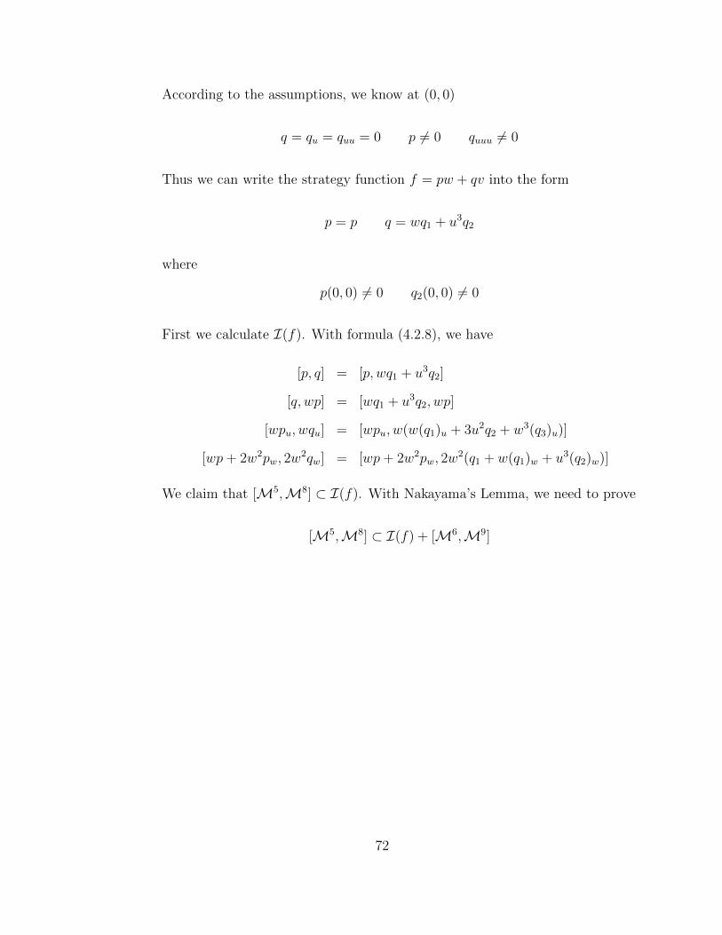
According to the assumptions, we know at (0, 0)

q = qu = quu = 0 p 6= 0 quuu 6= 0

Thus we can write the strategy function f = pw + qv into the form

p = p q = wq1 + u3q2

where

p(0, 0) 6= 0 q2(0, 0) 6= 0

First we calculate I(f). With formula (4.2.8), we have

[p, q] = [p, wq1 + u3q2]

[q, wp] = [wq1 + u3q2, wp]

[wpu, wqu] = [wpu, w(w(q1)u + 3u2q2 + w3(q3)u)]

[wp+ 2w2pw, 2w2qw] = [wp+ 2w2pw, 2w

2(q1 + w(q1)w + u3(q2)w)]

We claim that [M5,M8] ⊂ I(f). With Nakayama’s Lemma, we need to prove

[M5,M8] ⊂ I(f) + [M6,M9]

72

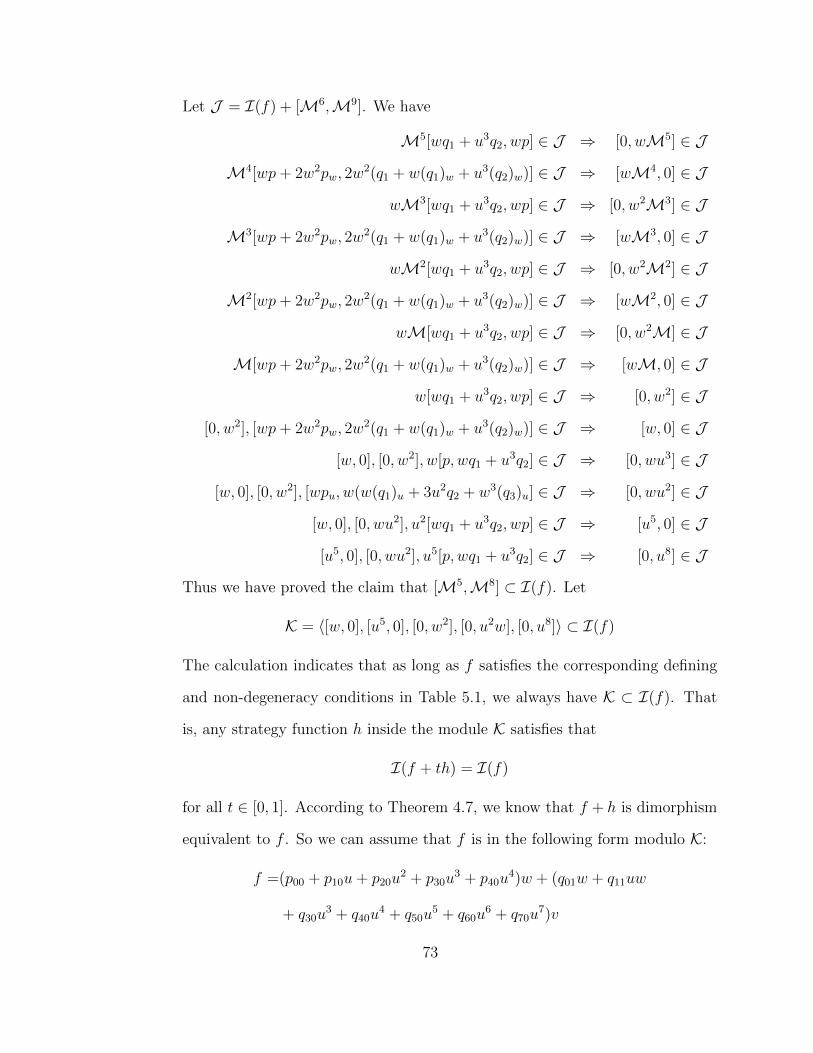
Let J = I(f) + [M6,M9]. We have

M5[wq1 + u3q2, wp] ∈ J ⇒ [0, wM5] ∈ J

M4[wp+ 2w2pw, 2w2(q1 + w(q1)w + u3(q2)w)] ∈ J ⇒ [wM4, 0] ∈ J

wM3[wq1 + u3q2, wp] ∈ J ⇒ [0, w2M3] ∈ J

M3[wp+ 2w2pw, 2w2(q1 + w(q1)w + u3(q2)w)] ∈ J ⇒ [wM3, 0] ∈ J

wM2[wq1 + u3q2, wp] ∈ J ⇒ [0, w2M2] ∈ J

M2[wp+ 2w2pw, 2w2(q1 + w(q1)w + u3(q2)w)] ∈ J ⇒ [wM2, 0] ∈ J

wM[wq1 + u3q2, wp] ∈ J ⇒ [0, w2M] ∈ J

M[wp+ 2w2pw, 2w2(q1 + w(q1)w + u3(q2)w)] ∈ J ⇒ [wM, 0] ∈ J

w[wq1 + u3q2, wp] ∈ J ⇒ [0, w2] ∈ J

[0, w2], [wp+ 2w2pw, 2w2(q1 + w(q1)w + u3(q2)w)] ∈ J ⇒ [w, 0] ∈ J

[w, 0], [0, w2], w[p, wq1 + u3q2] ∈ J ⇒ [0, wu3] ∈ J

[w, 0], [0, w2], [wpu, w(w(q1)u + 3u2q2 + w3(q3)u] ∈ J ⇒ [0, wu2] ∈ J

[w, 0], [0, wu2], u2[wq1 + u3q2, wp] ∈ J ⇒ [u5, 0] ∈ J

[u5, 0], [0, wu2], u5[p, wq1 + u3q2] ∈ J ⇒ [0, u8] ∈ J

Thus we have proved the claim that [M5,M8] ⊂ I(f). Let

K = 〈[w, 0], [u5, 0], [0, w2], [0, u2w], [0, u8]〉 ⊂ I(f)

The calculation indicates that as long as f satisfies the corresponding defining

and non-degeneracy conditions in Table 5.1, we always have K ⊂ I(f). That

is, any strategy function h inside the module K satisfies that

I(f + th) = I(f)

for all t ∈ [0, 1]. According to Theorem 4.7, we know that f + h is dimorphism

equivalent to f . So we can assume that f is in the following form modulo K:

f =(p00 + p10u+ p20u2 + p30u

3 + p40u4)w + (q01w + q11uw

+ q30u3 + q40u

4 + q50u5 + q60u

6 + q70u7)v

73

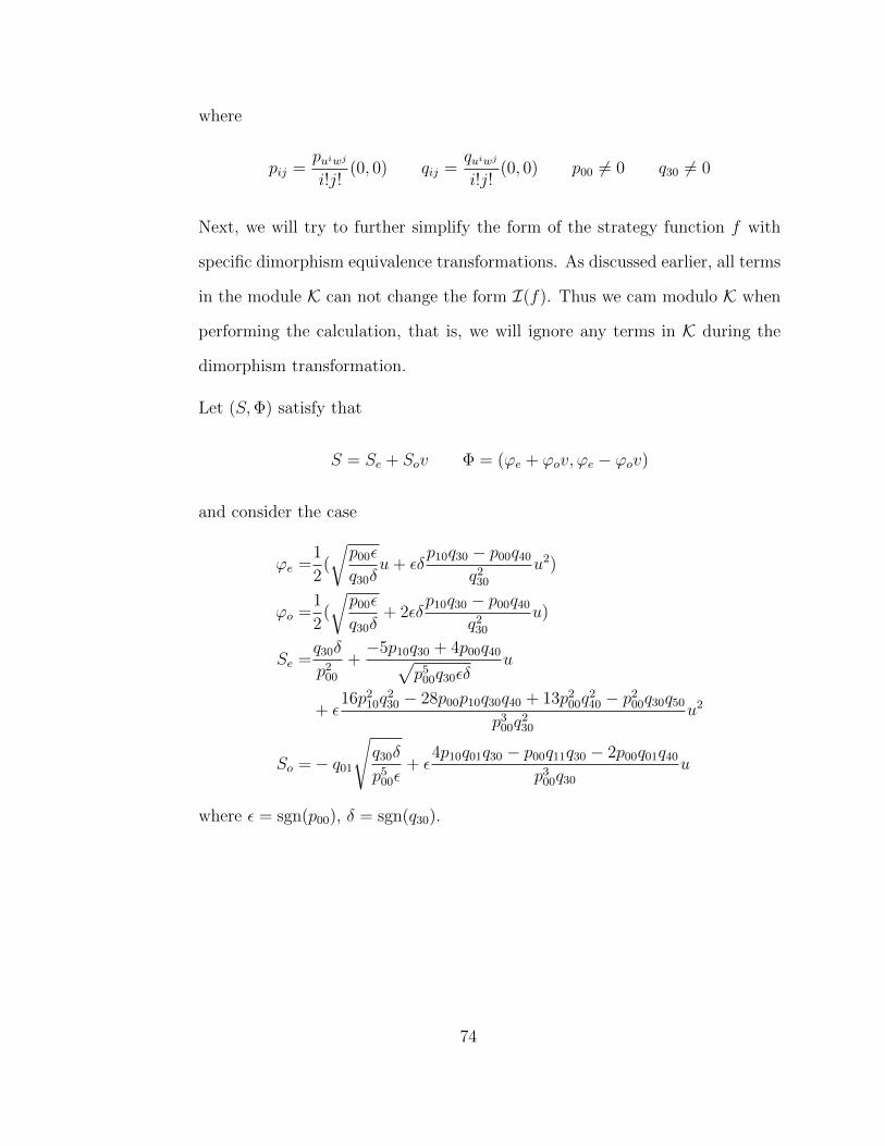
where

pij =puiwj

i!j!(0, 0) qij =

quiwj

i!j!(0, 0) p00 6= 0 q30 6= 0

Next, we will try to further simplify the form of the strategy function f with

specific dimorphism equivalence transformations. As discussed earlier, all terms

in the module K can not change the form I(f). Thus we cam modulo K when

performing the calculation, that is, we will ignore any terms in K during the

dimorphism transformation.

Let (S,Φ) satisfy that

S = Se + Sov Φ = (ϕe + ϕov, ϕe − ϕov)

and consider the case

ϕe =1

2(

√p00ε

q30δu+ εδ

p10q30 − p00q40

q230

u2)

ϕo =1

2(

√p00ε

q30δ+ 2εδ

p10q30 − p00q40

q230

u)

Se =q30δ

p200

+−5p10q30 + 4p00q40√

p500q30εδ

u

+ ε16p2

10q230 − 28p00p10q30q40 + 13p2

00q240 − p2

00q30q50

p300q

230

u2

So =− q01

√q30δ

p500ε

+ ε4p10q01q30 − p00q11q30 − 2p00q01q40

p300q30

u

where ε = sgn(p00), δ = sgn(q30).

74

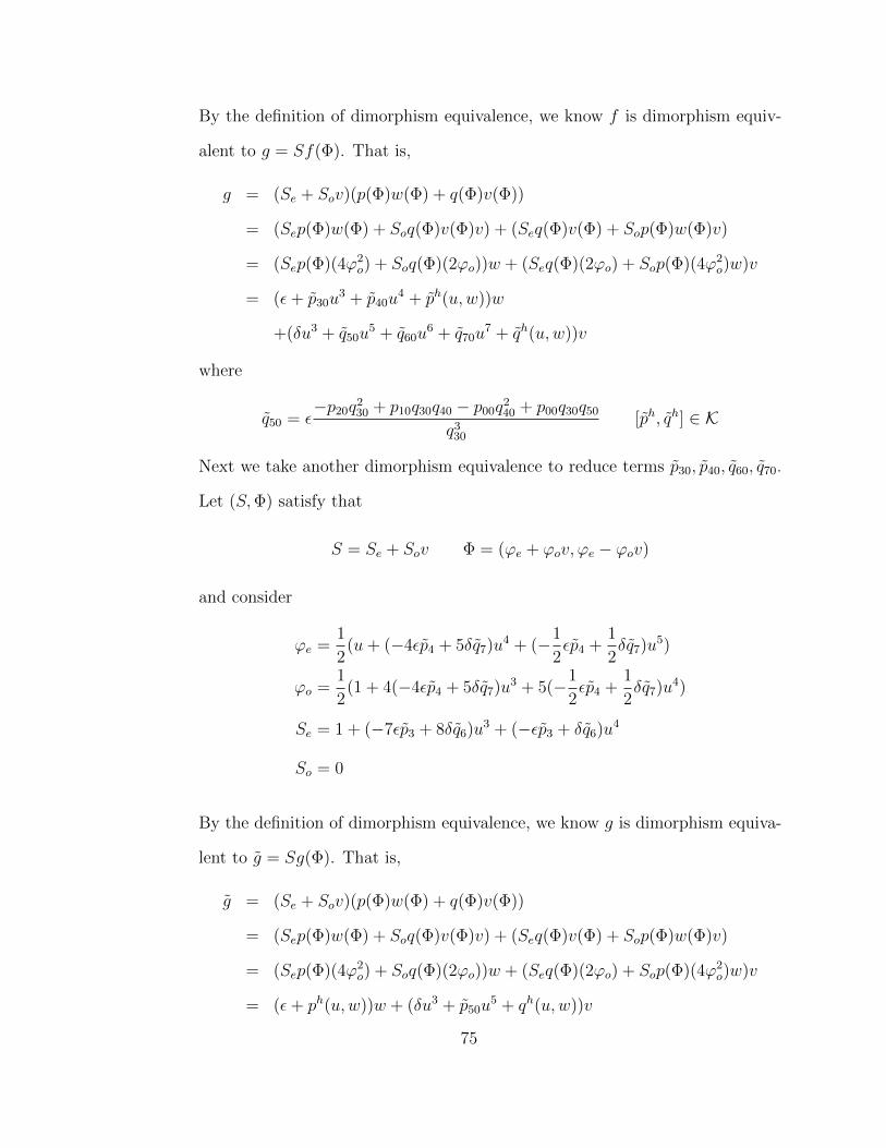
By the definition of dimorphism equivalence, we know f is dimorphism equiv-

alent to g = Sf(Φ). That is,

g = (Se + Sov)(p(Φ)w(Φ) + q(Φ)v(Φ))

= (Sep(Φ)w(Φ) + Soq(Φ)v(Φ)v) + (Seq(Φ)v(Φ) + Sop(Φ)w(Φ)v)

= (Sep(Φ)(4ϕ2o) + Soq(Φ)(2ϕo))w + (Seq(Φ)(2ϕo) + Sop(Φ)(4ϕ2

o)w)v

= (ε+ p30u3 + p40u

4 + ph(u,w))w

+(δu3 + q50u5 + q60u

6 + q70u7 + qh(u,w))v

where

q50 = ε−p20q

230 + p10q30q40 − p00q

240 + p00q30q50

q330

[ph, qh] ∈ K

Next we take another dimorphism equivalence to reduce terms p30, p40, q60, q70.

Let (S,Φ) satisfy that

S = Se + Sov Φ = (ϕe + ϕov, ϕe − ϕov)

and consider

ϕe =1

2(u+ (−4εp4 + 5δq7)u4 + (−1

2εp4 +

1

2δq7)u5)

ϕo =1

2(1 + 4(−4εp4 + 5δq7)u3 + 5(−1

2εp4 +

1

2δq7)u4)

Se = 1 + (−7εp3 + 8δq6)u3 + (−εp3 + δq6)u4

So = 0

By the definition of dimorphism equivalence, we know g is dimorphism equiva-

lent to g = Sg(Φ). That is,

g = (Se + Sov)(p(Φ)w(Φ) + q(Φ)v(Φ))

= (Sep(Φ)w(Φ) + Soq(Φ)v(Φ)v) + (Seq(Φ)v(Φ) + Sop(Φ)w(Φ)v)

= (Sep(Φ)(4ϕ2o) + Soq(Φ)(2ϕo))w + (Seq(Φ)(2ϕo) + Sop(Φ)(4ϕ2

o)w)v

= (ε+ ph(u,w))w + (δu3 + p50u5 + qh(u,w))v

75

where

q50 = ε−p20q

230 + p10q30q40 − p00q

240 + p00q30q50

q330

[ph, qh] ∈ K

This shows that g is dimorphism equivalent to g, so f is dimorphism equivalent

to

εw + (δu3 + µ0u5)v

where

ε = sgn(p) δ = sgn(qu3)

µ0 = ε− 1

12pu2q

2u3 + 1

144puqu3qu4 − 1

576pq2u4 + 1

720pqu3qu5

1216q3u3

At the end, we prove that if f = pw + qv is dimorphism equivalent to

εw + (δu3 + µ0u5)v

with the singularity at (0, 0), then the corresponding defining and non-degeneracy

conditions in Table 5.1 hold. The dimorphism equivalence indicates that there

exists a dimorphism equivalence transformation (S,Φ) such that f = Sh(Φ)

and we can write

S = Se + Sov Φ = (ϕe + ϕov, ϕe − ϕov)

where

Se > 0 ϕe = 0 (ϕe)u = ϕo > 0

at (0, 0). Then we have

f = pw + qv =[4εϕ2oSe + 2(8δϕ3

e + 32µ0ϕ5e)ϕoSo]w

+ [4ϕ2oεwSo + 2(8δd3 + 32µ0ϕ

5e)ϕowSe]v

Therefore,

p = 4εϕ2oSe + 2(8δϕ3

e + 32µ0ϕ5e)ϕoSo q = 4ϕ2

oεwSo + 2(8δϕ3e + 32µ0ϕ

5e)ϕowSe

76

So we know at (0, 0)

p = 4εϕ2oSe 6= 0 q = 0 qu = 0 quu = 0 quuu = 96δ(ϕe)

3u 6= 0

Now we have completely proved part (e).

(f) First, we show that f = pw + qv is dimorphism equivalent to

ε(uw + (α0w + β0u2)v)

if the corresponding defining and non-degeneracy conditions in Table 5.1 are

satisfied.

According to the assumptions, we can perform the dimorphism equivalence

(S,Φ) that satisfies

S =ε

pu(0, 0)Φ = Identity

where ε = sgn(pu(0, 0)). Then by the definition of dimorphism equivalence, we

know f is dimorphism equivalent to f = Sf(Φ). That is,

f = Sf(Φ) =ε

pu(0, 0)(pw + qv) = ε

p

pu(0, 0)w + ε

q

pu(0, 0)v

Define f = pw + qv, that is

p = εp

pu(0, 0)q = ε

q

pu(0, 0)

Now we assume that f = pw + qv satisfies the following form:

p = p10u+ p01w + p20u2 + p11uw + p30u

3 + ph(u,w)

q = q01w + q20u2 + q11uw + q02w

2 + q30u3 + q21u

2w + q40u4 + qh(u,w)

where

pij =ε

pu(0, 0)

puiwj

i!j!(0, 0) qij =

ε

pu(0, 0)

quiwj

i!j!(0, 0) ph ∈M2 qh ∈M3

77

and

phuu(0, 0) = phuw(0, 0) = phu3(0, 0) = 0

qhu3(0, 0) = qhu2w(0, 0) = qhu4(0, 0) = 0

One thing to point out here is that with direct calculation, we see

p10 = ε

Also with the assumptions in the theorem, we know that

q20 6= 0 q01 6= 0 p210 − 4q20q01 = 1− 4q20q01 6= 0

Let (S,Φ) satisfy that

S = Se + Sov Φ = (ϕe + ϕov, ϕe − ϕov)

where Se, So, ϕo, ϕe ∈ E . Note that in Proposition 4.2, we showed

u(Φ) = 2ϕe v(Φ) = 2ϕov w(Φ) = 4ϕ2ow

ϕe(0, 0) = 0 (ϕe)u(u, 0) = ϕo(u, 0)

Now consider the case

ϕe =1

2(u− −2q2

01q20p20 + 2q01q220p01 − q20p01 + q2

01q30ε+ q01q20q11ε

q20ε (4q01q20 − 1)w

− 2q01q220p20 − 2q3

20p01 − q20p20 − 3q01q20q30ε+ q220q11ε+ q30ε

q20ε (4q01q20 − 1)u2)

ϕo =1

2(1− 2q01q

220p20 − 2q3

20p01 − q20p20 − 3q01q20q30ε+ q220q11ε+ q30ε

q20ε (4q01q20 − 1)2u)

Se = 1 + [4 (2q01q

220p20 − 2q3

20p01 − q20p20 − 3q01q20q30ε+ q220q11ε+ q30ε)

q20ε (4q01q20 − 1)− q30

q20

]u

So = −2q01q20p20 + 2q220p01 − q01q30ε− q20q11ε

q20 (4q01q20 − 1)

78

By the definition of dimorphism equivalence, we know f is dimorphism equiv-

alent to g = Sf(Φ). That is,

g = (Se + Sov)(p(Φ)w(Φ) + q(Φ)v(Φ))

= (Sep(Φ)w(Φ) + Soq(Φ)v(Φ)v) + (Seq(Φ)v(Φ) + Sop(Φ)w(Φ)v)

= (Sep(Φ)(4ϕ2o) + Soq(Φ)(2ϕo))w + (Rq(Φ)(2ϕo) + Sop(Φ)(4ϕ2

o)w)v

= (εu+ p11uw + p30u3 + ph)w

+(q01w + q20u2 + q02w

2 + q21u2w + q40u

4 + qh)v

where ph ∈M2, qh ∈M3, and

phuu(0, 0) = phuw(0, 0) = ph3 (0, 0) = 0

qhu3(0, 0) = qhu2w(0, 0) = qh4 (0, 0) = 0

Now we have shown that a general strategy function f that satisfies the cor-

responding defining and non-degeneracy conditions in Table 5.1 is dimorphism

equivalent to the following strategy function:

g = (εu+ p11uw+ p30u3 + ph)w+ (q01w+ q20u

2 + q02w2 + q21u

2w+ q40u4 + qh)v

Next, let (S,Φ) satisfy that

S = Se + Sov Φ = (ϕe + ϕov, ϕe − ϕov)

and consider

ϕe =1

2(u− 2q201q

220p30−2q01q320p11−q01q20p30−3q201q20q40ε+q01q

220q21ε+q01q40ε+q

320q2ε

2q01q20ε(4q01q20−1)u3)

ϕo =1

2(1− 2q301q20p30−2q201q

220p11+q01q20p11−q301q40ε−q201q20q21ε+3q01q220q2ε−q20q2ε

q01q20ε(4q01q20−1)w

− 2q201q220p30−2q01q320p11−q01q20p30−3q201q20q40ε+q01q

220q21ε+q01q40ε+q

320q2ε

2q01q20ε(4q01q20−1)3u2)

Se = 1 + [3(2q301q20p30−2q201q

220p11+q01q20p11−q301q40ε−q201q20q21ε+3q01q220q2ε−q20q2ε)

q01q20ε(4q01q20−1)− q2

q01]w

− −10q201q220p30+10q01q320p11+5q01q20p30+23q201q20q40ε−5q01q220q21ε−7q01q40ε−5q320q2ε

2q01q20ε(4q01q20−1)u2

So = −2q201q20p30+2q01q220p11−q201q40ε−q01q20q21ε−q220q2εq01q20(4q01q20−1)

u

79

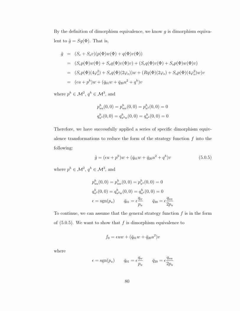
By the definition of dimorphism equivalence, we know g is dimorphism equiva-

lent to g = Sg(Φ). That is,

g = (Se + Sov)(p(Φ)w(Φ) + q(Φ)v(Φ))

= (Sep(Φ)w(Φ) + Soq(Φ)v(Φ)v) + (Seq(Φ)v(Φ) + Sop(Φ)w(Φ)v)

= (Sep(Φ)(4ϕ2o) + Soq(Φ)(2ϕo))w + (Rq(Φ)(2ϕo) + Sop(Φ)(4ϕ2

o)w)v

= (εu+ ph)w + (q01w + q20u2 + qh)v

where ph ∈M2, qh ∈M3, and

phuu(0, 0) = phuw(0, 0) = phu3(0, 0) = 0

qhu3(0, 0) = qhu2w(0, 0) = qhu4(0, 0) = 0

Therefore, we have successfully applied a series of specific dimorphism equiv-

alence transformations to reduce the form of the strategy function f into the

following:

g = (εu+ ph)w + (q01w + q20u2 + qh)v (5.0.5)

where ph ∈M2, qh ∈M3, and

phuu(0, 0) = phuw(0, 0) = phu3(0, 0) = 0

qhu3(0, 0) = qhu2w(0, 0) = qhu4(0, 0) = 0

ε = sgn(pu) q01 = εqwpu

q20 = εquu2pu

To continue, we can assume that the general strategy function f is in the form

of (5.0.5). We want to show that f is dimorphism equivalence to

f0 = εuw + (q01w + q20u2)v

where

ε = sgn(pu) q01 = εqwpu

q20 = εquu2pu

80

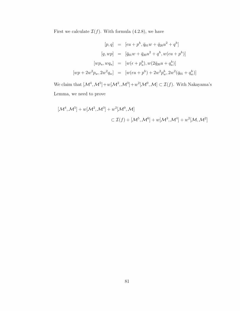
First we calculate I(f). With formula (4.2.8), we have

[p, q] = [εu+ ph, q01w + q20u2 + qh]

[q, wp] = [q01w + q20u2 + qh, w(εu+ ph)]

[wpu, wqu] = [w(ε+ phu), w(2q20u+ qhu)]

[wp+ 2w2pw, 2w2qw] = [w(εu+ ph) + 2w2phw, 2w

2(q01 + qhw)]

We claim that [M4,M5]+w[M2,M3]+w2[M0,M] ⊂ I(f). With Nakayama’s

Lemma, we need to prove

[M4,M5] + w[M2,M3] + w2[M0,M]

⊂ I(f) + [M5,M6] + w[M3,M4] + w2[M,M2]

81

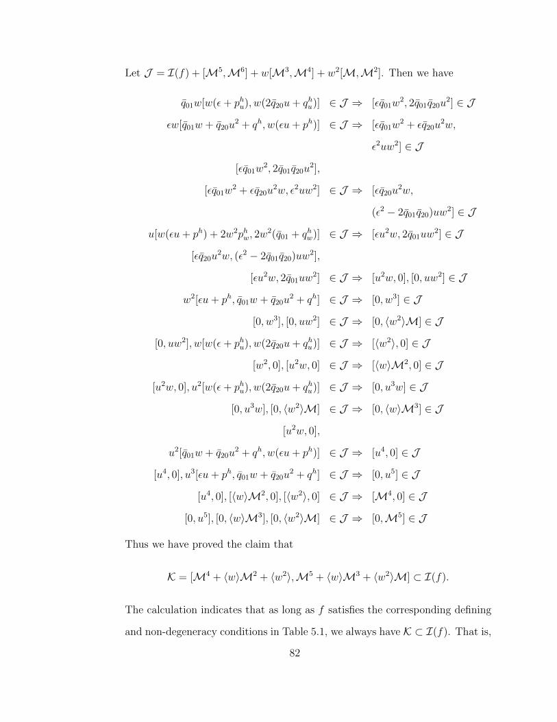
Let J = I(f) + [M5,M6] + w[M3,M4] + w2[M,M2]. Then we have

q01w[w(ε+ phu), w(2q20u+ qhu)] ∈ J ⇒ [εq01w2, 2q01q20u

2] ∈ J

εw[q01w + q20u2 + qh, w(εu+ ph)] ∈ J ⇒ [εq01w

2 + εq20u2w,

ε2uw2] ∈ J

[εq01w2, 2q01q20u

2],

[εq01w2 + εq20u

2w, ε2uw2] ∈ J ⇒ [εq20u2w,

(ε2 − 2q01q20)uw2] ∈ J

u[w(εu+ ph) + 2w2phw, 2w2(q01 + qhw)] ∈ J ⇒ [εu2w, 2q01uw

2] ∈ J

[εq20u2w, (ε2 − 2q01q20)uw2],

[εu2w, 2q01uw2] ∈ J ⇒ [u2w, 0], [0, uw2] ∈ J

w2[εu+ ph, q01w + q20u2 + qh] ∈ J ⇒ [0, w3] ∈ J

[0, w3], [0, uw2] ∈ J ⇒ [0, 〈w2〉M] ∈ J

[0, uw2], w[w(ε+ phu), w(2q20u+ qhu)] ∈ J ⇒ [〈w2〉, 0] ∈ J

[w2, 0], [u2w, 0] ∈ J ⇒ [〈w〉M2, 0] ∈ J

[u2w, 0], u2[w(ε+ phu), w(2q20u+ qhu)] ∈ J ⇒ [0, u3w] ∈ J

[0, u3w], [0, 〈w2〉M] ∈ J ⇒ [0, 〈w〉M3] ∈ J

[u2w, 0],

u2[q01w + q20u2 + qh, w(εu+ ph)] ∈ J ⇒ [u4, 0] ∈ J

[u4, 0], u3[εu+ ph, q01w + q20u2 + qh] ∈ J ⇒ [0, u5] ∈ J

[u4, 0], [〈w〉M2, 0], [〈w2〉, 0] ∈ J ⇒ [M4, 0] ∈ J

[0, u5], [0, 〈w〉M3], [0, 〈w2〉M] ∈ J ⇒ [0,M5] ∈ J

Thus we have proved the claim that

K = [M4 + 〈w〉M2 + 〈w2〉,M5 + 〈w〉M3 + 〈w2〉M] ⊂ I(f).

The calculation indicates that as long as f satisfies the corresponding defining

and non-degeneracy conditions in Table 5.1, we always have K ⊂ I(f). That is,

82

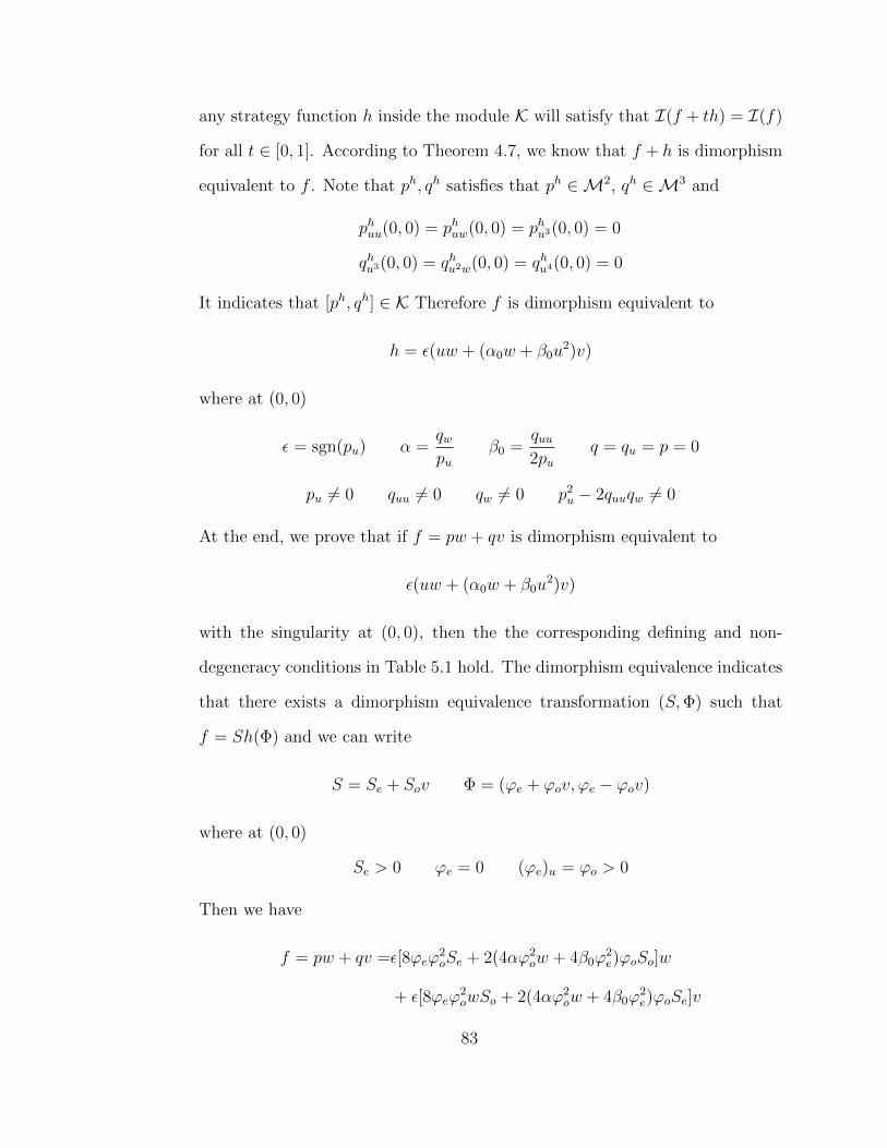
any strategy function h inside the module K will satisfy that I(f + th) = I(f)

for all t ∈ [0, 1]. According to Theorem 4.7, we know that f + h is dimorphism

equivalent to f . Note that ph, qh satisfies that ph ∈M2, qh ∈M3 and

phuu(0, 0) = phuw(0, 0) = phu3(0, 0) = 0

qhu3(0, 0) = qhu2w(0, 0) = qhu4(0, 0) = 0

It indicates that [ph, qh] ∈ K Therefore f is dimorphism equivalent to

h = ε(uw + (α0w + β0u2)v)

where at (0, 0)

ε = sgn(pu) α =qwpu

β0 =quu2pu

q = qu = p = 0

pu 6= 0 quu 6= 0 qw 6= 0 p2u − 2quuqw 6= 0

At the end, we prove that if f = pw + qv is dimorphism equivalent to

ε(uw + (α0w + β0u2)v)

with the singularity at (0, 0), then the the corresponding defining and non-

degeneracy conditions in Table 5.1 hold. The dimorphism equivalence indicates

that there exists a dimorphism equivalence transformation (S,Φ) such that

f = Sh(Φ) and we can write

S = Se + Sov Φ = (ϕe + ϕov, ϕe − ϕov)

where at (0, 0)

Se > 0 ϕe = 0 (ϕe)u = ϕo > 0

Then we have

f = pw + qv =ε[8ϕeϕ2oSe + 2(4αϕ2

ow + 4β0ϕ2e)ϕoSo]w

+ ε[8ϕeϕ2owSo + 2(4αϕ2

ow + 4β0ϕ2e)ϕoSe]v

83

Therefore,

p = 8εϕeϕ2oSe + 2ε(4αϕ2

ow + 4β0ϕ2e)ϕoSo

q = 8εϕeϕ2owSo + 2ε(4αϕ2

ow + 4β0ϕ2e)ϕoSe

So we know at (0, 0)

p = 0 q = 0 qu = 0

quu = 16εβ0(ϕe)2uϕoSe 6= 0 pu = 8ε(ϕe)uϕ

2oSe 6= 0

p2u−2quuqw = 64(ϕe)

3uϕ

4oS

2e−32β0(ϕe)

2uϕoSe ·8αϕ3

o = 64(ϕe)2uϕ

4oS

2e (1−4αβ0) 6= 0

Now we have completely proved part (f).

Remark 5.4. In the proof of Theorem 5.1 we calculate the strong dimorphism equiva-

lence restricted tangent space I(f) for strategy functions f satisfying certain defining

and non-degeneracy conditions. The result enables us to prove that these f are di-

morphism equivalent to the given normal forms h. When we find universal unfoldings

of h in Chapter 6 we will need to know RT (h).

Lemma 5.5. The restricted tangent spaces for the normal forms in Theorem 5.1 are

given in Table 5.2.

Proof. (a) It follows from Proposition 4.2 that the dimorphism equivalence re-

stricted tangent space of the strategy function h = ε(w + µ0uv) is

RT (h) = 〈[0, w], [0, u2], [u, 0], [w, 0]〉+ R{[1, µ0u]}

= [M,M2] + w[M0,M0] + R{[1, µ0u]}

84

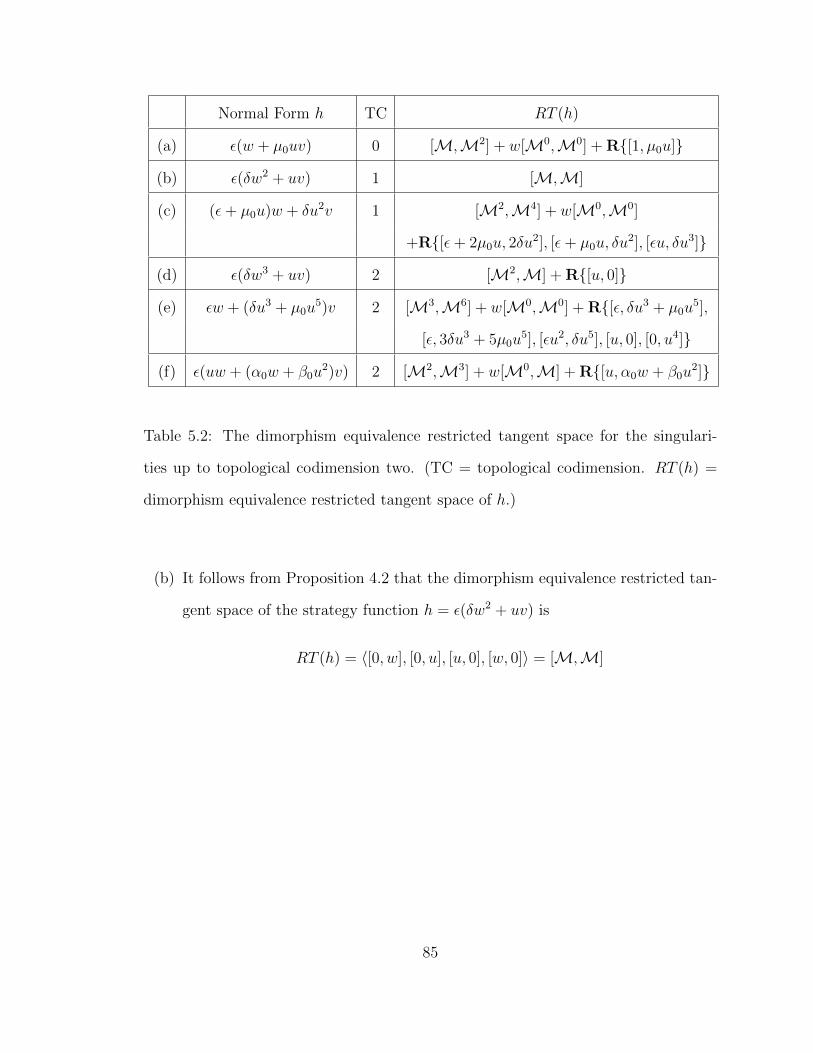
Normal Form h TC RT (h)

(a) ε(w + µ0uv) 0 [M,M2] + w[M0,M0] + R{[1, µ0u]}

(b) ε(δw2 + uv) 1 [M,M]

(c) (ε+ µ0u)w + δu2v 1 [M2,M4] + w[M0,M0]

+R{[ε+ 2µ0u, 2δu2], [ε+ µ0u, δu

2], [εu, δu3]}

(d) ε(δw3 + uv) 2 [M2,M] + R{[u, 0]}

(e) εw + (δu3 + µ0u5)v 2 [M3,M6] + w[M0,M0] + R{[ε, δu3 + µ0u

5],

[ε, 3δu3 + 5µ0u5], [εu2, δu5], [u, 0], [0, u4]}

(f) ε(uw + (α0w + β0u2)v) 2 [M2,M3] + w[M0,M] + R{[u, α0w + β0u

2]}

Table 5.2: The dimorphism equivalence restricted tangent space for the singulari-

ties up to topological codimension two. (TC = topological codimension. RT (h) =

dimorphism equivalence restricted tangent space of h.)

(b) It follows from Proposition 4.2 that the dimorphism equivalence restricted tan-

gent space of the strategy function h = ε(δw2 + uv) is

RT (h) = 〈[0, w], [0, u], [u, 0], [w, 0]〉 = [M,M]

85

(c) It follows from Proposition 4.2 that the dimorphism equivalence restricted tan-

gent space of the strategy function h = (ε+ µ0u)w + δu2v is

RT (h) = I(h) + R{[ε+ 2µ0u, 2δu2], [2εu+ 3µ0u

2, 2δu3], [3εu2, 2δu4]}

= 〈[u3, 0], [w, 0], [0, u5], [0, uw], [0, w2]〉

+R{[ε+ 2µ0u, 2δu2], [ε+ µ0u, δu

2], [εu, δu3], [u2, 0], [0, u4], [0, w]}

= 〈[u2, 0], [w, 0], [0, u4], [0, w]〉

+R{[ε+ 2µ0u, 2δu2], [ε+ µ0u, δu

2], [εu, δu3]}

= [M2,M4] + w[M0,M0]

+R{[ε+ 2µ0u, 2δu2], [ε+ µ0u, δu

2], [εu, δu3]}

(d) It follows from Proposition 4.2 that the dimorphism equivalence restricted tan-

gent space of the strategy function h = ε(δw3 + uv) is

RT (h) = I(h) + R[5δw2, u] = [M2,M] + R{[u, 0]}

(e) It follows from Proposition 4.2 that the dimorphism equivalence restricted tan-

gent space of the strategy function h = εw + (δu3 + µ0u5)v is

RT (h) = I(h) + R{[ε, 3δu3 + 5µ0u5], [2εu, 3δu4 + 5µ0u

6],

[3εu2, 3δu5 + 5µ0u7], [4εu3, 3δu6], [5εu4, 3δu7]}

= 〈[w, 0], [u5, 0], [0, w2], [0, u2w], [0, u8]+〉

+R{[ε, δu3 + µ0u5], [εu, δu4 + µ0u

6], [εu2, δu5 + µ0u7], [εu3, δu6],

[εu4, δu7], [δu3, εw], [δu4, εuw], [ε, 3δu3 + 5µ0u5], [2εu, 3δu4 + 5µ0u

6],

[3εu2, 3δu5 + 5µ0u7], [4εu3, 3δu6], [5εu4, 3δu7]}

= 〈[w, 0], [u3, 0], [0, w], [0, u6]〉

+R{[ε, δu3 + µ0u5], [ε, 3δu3 + 5µ0u

5], [εu2, δu5], [u, 0], [0, u4]}

= [M3,M6] + w[M0,M0]

+R{[ε, δu3 + µ0u5], [ε, 3δu3 + 5µ0u

5], [εu2, δu5], [u, 0], [0, u4]}

86

(f) It follows from Proposition 4.2 that the dimorphism equivalence restricted tan-

gent space of the strategy function h = ε(uw + (α0w + β0u2)v) is

RT (h) = I(h) + R{[3u2, 2β0u3 + 4α0uw],

[4u3, 2β0u4 + 6α0u

2w], [2u, 2β0u2 + 2α0w]}

= [M4,M5] + w[M2,M3] + w2[M0,M] + R{[u, β0u2 + α0w],

[uw, β0u2w + α0w

2], [u2, β0u3 + α0uw], [u3, β0u

4 + α0u2w],

[α0w + β0u2, uw], [α0uw + β0u

3, u2w], [w, 2β0uw], [uw, 2β0u2w],

[uw, 2α0w2], [3u2, 2β0u

3 + 4α0uw], [4u3, 2β0u4 + 6α0u

2w]}

= [M2,M3] + w[M0,M] + R{[u, α0w + β0u2]}

87

CHAPTER 6

UNIVERSAL UNFOLDINGS UNDER DIMORPHISM

EQUIVALENCE

In this chapter we develop the universal unfolding theory in the context of dimorphism

equivalence. First we define universal unfolding and codimension (see Definition 6.4).

Then we define the dimorphism equivalence tangent space and state the universal

unfolding theorem in singularity theory (see Theorem 6.7). This theorem is a special

case of a general theorem proved by Damon [2]. At the end, we apply the univer-

sal unfolding theorem to calculate the universal unfoldings for singularities up to

topological codimension two in Theorem 6.9.

6.1 Preliminary Definitions

In this section, we define a few concepts in universal unfolding theory of strategy

functions. All of these definitions can be found in [14].

Definition 6.1. Let f be a C∞ strategy function R2 → R defined on a neighborhood

of the origin. Then F : R2 ×Rk → R is a k-parameter unfolding of f if

F (x, y, 0) = f(x, y) F (x, x, α) = 0

where the parameter α ∈ Rk.

Suppose F (x, y, α) (α ∈ Rk) and H(x, y, β) (β ∈ Rl) are unfoldings of f . We

88

say that the perturbations of the H unfolding are contained in the F unfolding if for

every β ∈ Rl, there exists A(β) ∈ Rk such that F (·, ·, A(β)) is dimorphism equivalent

to H(·, ·, β). We formalize this in Definition 6.2.

Definition 6.2. Let F (x, y, α) be a k-parameter unfolding of f and let H(x, y, β) be

an l-parameter unfolding of f . We say that H factors through F if there exists maps

S : R2 ×Rl → R, Φ : R2 ×Rl → R2, and A : Rl → Rk such that

H(x, y, β) = S(x, y, β)F (Φ(x, y, β), A(β))

where

1. S(x, y, 0) = 1

2. Φ(x, y, 0) = (x, y)

3. Φ(x, y, β) = (ϕ(x, y, β), ϕ(y, x, β)) where ϕ : R2 ×Rl → R

4. (dΦ)x,x,β = c(x, β)I2 where c(x, β) > 0

5. A(0) = 0

Remark 6.3. We do not require that Φ(0, 0, β) = (0, 0); that is, when β is nonzero,

the equivalence need not preserve the origin.

There are unfoldings F that contains all perturbations of f , up to dimorphism

equivalence. These unfoldings are characterized in Definition 6.4.

Definition 6.4. An unfolding F of f is versal if every unfolding of f factors through

F . A versal unfolding depending on the minimum number of parameters is called

universal. That minimum number is called the C∞ codimension of f . In addition,

the topological codimension of f is the C∞ codimension of f minus the number of

modal parameters in the universal unfolding F .

89

Suppose F (x, y, α) is a universal unfolding of a strategy function f . This implies

that every one-parameter unfolding of f can factor through F . For any strategy

function perturbation η(x, y), consider the one-parameter unfolding

H(x, y, t) = f(x, y) + tη(x, y)

Since H factors through F , we can write

H(x, y, t) = S(x, y, t)F (Φ(x, y, t), A(t)) (6.1.1)

where S,Φ, A satisfy the conditions in Definition 6.2.

On differentiating (6.1.1) with respect to t and evaluating at t = 0, we have

η(x, y) = S(x, y, 0)f(x, y) + ϕ(x, y, 0)Fx(x, y, 0)

+ ϕ(y, x, 0)Fy(x, y, 0) +k∑i=1

AiFαi(x, y, 0)

(6.1.2)

where A(t) = (A1(t), . . . , Ak(t)) and · is differentiation with respect to t.

6.2 Dimorphism Equivalence Tangent Space

Definition 6.5. The dimorphism equivalence tangent space of a strategy function f ,

denoted by T (f), is the set of all η(x, y) of the form given in the first three terms on

the right hand side of (6.1.2), where (S,Φ) satisfies all assumptions in Definition 6.2.

Remark 6.6. The only difference between the definition of T (f) and RT (f) is the

fact stated in Remark 6.3 that Φ in the definition of T (f) does not need to fix

the origin for different parameter values, but Φ in the definition of RT (f) needs to

fix the origin for all parameters. Therefore, with similar calculation performed in

Proposition 4.2, we can have

T (f) = RT (f) + R{[pu, qu]} (6.2.1)

Thus, RT (f) has finite codimension if and only if T (f) has finite codimension.

90

The structure of T (f) leads to a necessary condition for F to be a universal

unfolding of f . Specifically, if an unfolding F is versal, then

E2 = T (f) + R{Fα1(x, y, 0), . . . , Fαk(x, y, 0)} (6.2.2)

An important result in singularity theory states that (6.2.2) is also a sufficient

condition for F to be a universal unfolding. See §9 in [2].

Theorem 6.7. Let F be a k-parameter unfolding of f . Then F is a versal unfolding

of f if and only if

E2 = T (f) + R{ ∂G∂α1

(x, y, 0), . . . ,∂G

∂αk(x, y, 0)} (6.2.3)

Corollary 6.8. An unfolding F of f is universal if and only if the sum in (6.2.3) is

a direct sum. The number of parameters in F equals the codimension of T (f). In

particular, if f has C∞ codimension k and z1, . . . , zk ∈ E2 are chosen so that

E2 = T (f)⊕R{z1, . . . , zk}

then

F (x, y, α) = f(x, y) + α1z1(x, y) + · · ·+ αkzk(x, y)

is a universal unfolding of f .

6.3 Universal Unfoldings of Low Codimension Singularities

In this section, we calculation the universal unfolding for each singularities up to

topological codimension two.

Theorem 6.9. Table 6.1 gives a universal unfolding for each normal form in Theo-

rem 5.1.

91

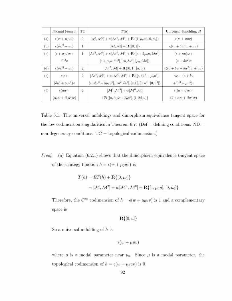
Normal Form h TC T (h) Universal Unfolding H

(a) ε(w + µ0uv) 0 [M,M2] + w[M0,M0] + R{[1, µ0u], [0, µ0]} ε(w + µuv)

(b) ε(δw2 + uv) 1 [M,M] + R{[0, 1]} ε((a+ δw)w + uv)

(c) (ε+ µ0u)w+ 1 [M2,M4] + w[M0,M0] + R{[ε+ 2µ0u, 2δu2], (ε+ µu)w+

δu2v [ε+ µ0u, δu2], [εu, δu3], [µ0, 2δu]} (a+ δu2)v

(d) ε(δw3 + uv) 2 [M2,M] + R{[0, 1], [u, 0]} ε((a+ bw + δw2)w + uv)

(e) εw+ 2 [M3,M6] + w[M0,M0] + R{[ε, δu3 + µ0u5], εw + (a+ bu

(δu3 + µ0u5)v [ε, 3δu3 + 5µ0u

5], [εu2, δu5], [u, 0], [0, u4], [0, u2]} +δu3 + µu5)v

(f) ε(uw+ 2 [M2,M3] + w[M0,M] ε((a+ u)w+

(α0w + β0u2)v) +R{[u, α0w + β0u

2], [1, 2β0u]} (b+ αw + βu2)v)

Table 6.1: The universal unfoldings and dimorphism equivalence tangent space for

the low codimension singularities in Theorem 6.7. (Def = defining conditions. ND =

non-degeneracy conditions. TC = topological codimension.)

Proof. (a) Equation (6.2.1) shows that the dimorphism equivalence tangent space

of the strategy function h = ε(w + µ0uv) is

T (h) = RT (h) + R{[0, µ0]}

= [M,M2] + w[M0,M0] + R{[1, µ0u], [0, µ0]}

Therefore, the C∞ codimension of h = ε(w + µ0uv) is 1 and a complementary

space is

R{[0, u]}

So a universal unfolding of h is

ε(w + µuv)

where µ is a modal parameter near µ0. Since µ is a modal parameter, the

topological codimension of h = ε(w + µ0uv) is 0.

92

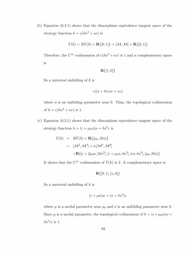
(b) Equation (6.2.1) shows that the dimorphism equivalence tangent space of the

strategy function h = ε(δw2 + uv) is

T (h) = RT (h) + R{[0, 1]} = [M,M] + R{[0, 1]}

Therefore, the C∞ codimension of ε(δw2 + uv) is 1 and a complementary space

is

R{[1, 0]}

So a universal unfolding of h is

ε((a+ δw)w + uv)

where a is an unfolding parameter near 0. Thus, the topological codimension

of h = ε(δw2 + uv) is 1.

(c) Equation (6.2.1) shows that the dimorphism equivalence tangent space of the

strategy function h = (ε+ µ0u)w + δu2v is

T (h) = RT (h) + R{[µ0, 2δu]}

= [M2,M4] + w[M0,M0]

+R{[ε+ 2µ0u, 2δu2], [ε+ µ0u, δu

2], [εu, δu3], [µ0, 2δu]}

It shows that the C∞ codimension of T (h) is 2. A complementary space is

R{[0, 1], [u, 0]}

So a universal unfolding of h is

(ε+ µu)w + (a+ δu2)v

where µ is a modal parameter near µ0 and a is an unfolding parameter near 0.

Since µ is a modal parameter, the topological codimension of h = (ε+µ0u)w+

δu2v) is 1.

93

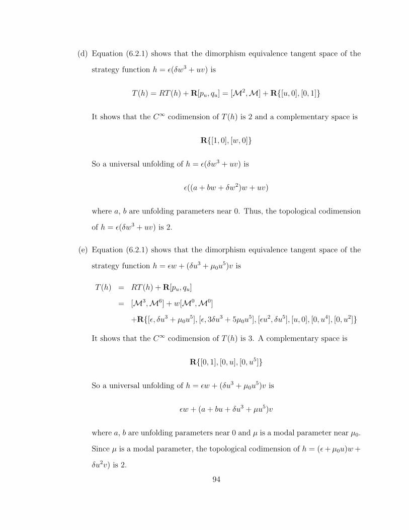
(d) Equation (6.2.1) shows that the dimorphism equivalence tangent space of the

strategy function h = ε(δw3 + uv) is

T (h) = RT (h) + R[pu, qu] = [M2,M] + R{[u, 0], [0, 1]}

It shows that the C∞ codimension of T (h) is 2 and a complementary space is

R{[1, 0], [w, 0]}

So a universal unfolding of h = ε(δw3 + uv) is

ε((a+ bw + δw2)w + uv)

where a, b are unfolding parameters near 0. Thus, the topological codimension

of h = ε(δw3 + uv) is 2.

(e) Equation (6.2.1) shows that the dimorphism equivalence tangent space of the

strategy function h = εw + (δu3 + µ0u5)v is

T (h) = RT (h) + R[pu, qu]

= [M3,M6] + w[M0,M0]

+R{[ε, δu3 + µ0u5], [ε, 3δu3 + 5µ0u

5], [εu2, δu5], [u, 0], [0, u4], [0, u2]}

It shows that the C∞ codimension of T (h) is 3. A complementary space is

R{[0, 1], [0, u], [0, u5]}

So a universal unfolding of h = εw + (δu3 + µ0u5)v is

εw + (a+ bu+ δu3 + µu5)v

where a, b are unfolding parameters near 0 and µ is a modal parameter near µ0.

Since µ is a modal parameter, the topological codimension of h = (ε+µ0u)w+

δu2v) is 2.

94

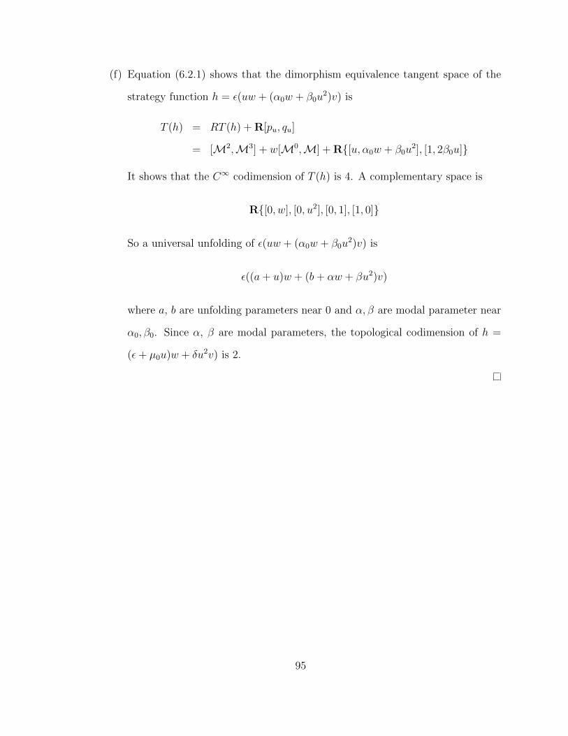
(f) Equation (6.2.1) shows that the dimorphism equivalence tangent space of the

strategy function h = ε(uw + (α0w + β0u2)v) is

T (h) = RT (h) + R[pu, qu]

= [M2,M3] + w[M0,M] + R{[u, α0w + β0u2], [1, 2β0u]}

It shows that the C∞ codimension of T (h) is 4. A complementary space is

R{[0, w], [0, u2], [0, 1], [1, 0]}

So a universal unfolding of ε(uw + (α0w + β0u2)v) is

ε((a+ u)w + (b+ αw + βu2)v)

where a, b are unfolding parameters near 0 and α, β are modal parameter near

α0, β0. Since α, β are modal parameters, the topological codimension of h =

(ε+ µ0u)w + δu2v) is 2.

95

CHAPTER 7

THE RECOGNITION PROBLEM FOR UNIVERSAL

UNFOLDINGS

In this chapter, we consider the following question that is called the recognition prob-

lem for universal unfoldings: Let F (x, y, α) be an unfolding of a strategy function

f(x, y), where f is dimorphism equivalent to a normal form h. When is F a universal

unfolding of f? This situation usually arises in applications. We use the approach de-

veloped by Golubitsky and Schaeffer [12] to answer this question for low codimension

bifurcation problems. The results are summarized in Theorem 7.7 for the strategy

function singularities up to topological codimension one.

Let γ = (S,Φ) be a dimorphism equivalence. That is, S and Φ satisfy conditions

in Definition 3.3. Denote

γ(h)(x, y) = S(x, y)h(Φ(x, y))

Lemma 7.1. Suppose f = γ(h). Then

T (f) = γ(T (h))

Proof. Define a smooth curve of dimorphism equivalences δt at h as

δt(h) = S(x, y, t)h(Φ(x, y, t))

where S,Φ vary smoothly in t. Assume that

S(x, y, 0) = 1 Φ(x, y, 0) = (x, y)

96

In other words, δ0 is the identity map. Then g =d

dtδt(h)|t=0 is a typical member of

T (h). With direct calculation,

γ(g) = γd

dtδt(h)|t=0 =

d

dtγ(δt(h))|t=0

=d

dtγδtγ

−1γ(h)|t=0

=d

dtγδtγ

−1(f))|t=0

Let δt = γδtγ−1. Then δ0 is the identity map and δt is a smooth curve of dimorphism

equivalences at f such that

γ(g) =d

dtδt(f)|t=0

In other words, γ(g) ∈ T (f) and therefore

γ(T (h)) ⊂ T (f)

Interchanging the roles of f and h shows that

T (f) ⊂ γ(T (h))

and the equality holds as claimed.

Define the pullback mapping Φ∗ as

Φ∗(f)(x, y) := f(Φ(x, y))

Note that in this thesis, we consistently use the coordinates (u, v) instead of (x, y).

Therefore, we assume that from now on, the strategy functions are respective to the

coordinates (u, v).

Lemma 7.2. Let I = 〈[p1, q1], · · · , [pk, qk]〉. Then Φ∗(I) is the module

〈Φ∗([p1, q1]), · · · ,Φ∗([pk, qk])〉

97

Proof. Follows from the fact that if f1, f2 are strategy functions, then

Φ∗(f1 + f2) = Φ∗(f1) + Φ∗(f2)

Remark 7.3. If I, J are modules, then Lemma 7.2 implies that

Φ∗(I + J ) = Φ∗(I) + Φ∗(J )

Next, we show that the modules ws[Mk,Mk] and ws[Mk,Mk+1] are invariant

under pullback maps which come from dimorphism equivalences that fix the origin

(0, 0).

Definition 7.4. An module I is intrinsic if for every dimorphism equivalence γ =

(S,Φ) such that Φ(0) = 0, we have γ(I) = I.

Proposition 7.5. The modules ws[Mk,Mk] and ws[Mk,Mk+1] are intrinsic, where

k, s are non-negative intergers.

Proof. Note that under the (u, v) coordinate, we can write

S = Se + Sov Φ = (ϕe + ϕov, ϕe − ϕov)

where Se, So, ϕe, ϕo ∈ E . Assume that

f = pw + qv = [p, q] ∈ [Mk,Mk]

then we see that

S · f = (Se + Sov)(pw + qv)

= (Sep+ Soq)w + (Seq + Sopw)v

= [Sep+ Soq, Seq + Sopw]

f ◦ Φ = p(2ϕe, 4ϕ2ow)4ϕ2

ow + q(2ϕe, 4ϕ2ow)2ϕov

= [p(2ϕe, 4ϕ2ow)4ϕ2

o, q(2ϕe, 4ϕ2ow)2ϕo]

98

Since So, Se, ϕe, ϕo ∈M0, p, q ∈Mk, we have

S · f ∈ [Mk,Mk] f ◦ Φ ∈ [Mk,Mk]

Similarly, if we assume that

f = [p, q] = pw + qv ∈ ws[Mk,Mk+1]

then we have

S · f ∈ ws[Mk,Mk+1] f ◦ Φ ∈ ws[Mk,Mk]

Hence, the proof is done.

Remark 7.6. Proposition 7.5 implies that the modules

J1 = [Mk0 ,Mk0 ] + · · ·+ ws[Mks ,Mks ] + [M l0 ,M l0+1] + · · ·+ wt[M lt ,M lt+1]

are intrinsic for any finite set of nonnegative integers s, t, ki, lj where i = 0, . . . , s

and j = 0, . . . , t.

Let h be a normal form of f (= [p, q]). We now calculate necessary conditions for

F to be a universal unfolding of f when f = γ(h). We do this in the following way:

(a) Write

T (h) = J ⊕ Vh

where J is intrinsic.

(b) Using Lemma 7.1 and the fact that J is intrinsic, write

T (f) = J ⊕ Vf

(c) By Theorem 6.7, F is a k-parameter universal unfolding of f (where k is the

C∞ codimension of h ) if and only if

E2 = J ⊕ Vf ⊕R{Fα1 , . . . , Fαk}

99

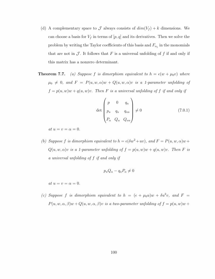
(d) A complementary space to J always consists of dim(Vf ) + k dimensions. We

can choose a basis for Vf in terms of [p, q] and its derivatives. Then we solve the

problem by writing the Taylor coefficients of this basis and Fαjin the monomials

that are not in J . It follows that F is a universal unfolding of f if and only if

this matrix has a nonzero determinant.

Theorem 7.7. (a) Suppose f is dimorphism equivalent to h = ε(w + µ0v) where

µ0 6= 0, and F = P (u,w, α)w + Q(u,w, α)v is a 1-parameter unfolding of

f = p(u,w)w + q(u,w)v. Then F is a universal unfolding of f if and only if

det

p 0 qu

pu qu quu

Pα Qα Qαu

6= 0 (7.0.1)

at u = v = α = 0.

(b) Suppose f is dimorphism equivalent to h = ε(δw2 +uv), and F = P (u,w, α)w+

Q(u,w, α)v is a 1-parameter unfolding of f = p(u,w)w + q(u,w)v. Then F is

a universal unfolding of f if and only if

puQα − quPα 6= 0

at u = v = α = 0.

(c) Suppose f is dimorphism equivalent to h = (ε + µ0u)w + δu2v, and F =

P (u,w, α, β)w+Q(u,w, α, β)v is a two-parameter unfolding of f = p(u,w)w+

100

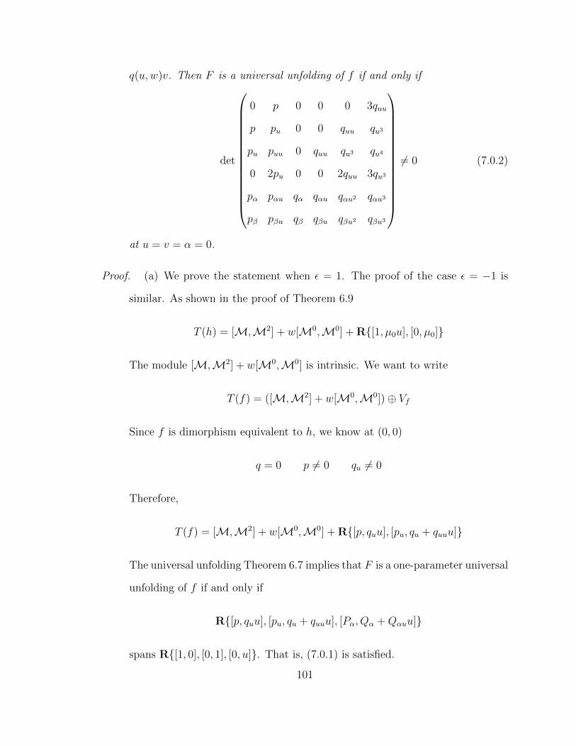
q(u,w)v. Then F is a universal unfolding of f if and only if

det

0 p 0 0 0 3quu

p pu 0 0 quu qu3

pu puu 0 quu qu3 qu4

0 2pu 0 0 2quu 3qu3

pα pαu qα qαu qαu2 qαu3

pβ pβu qβ qβu qβu2 qβu3

6= 0 (7.0.2)

at u = v = α = 0.

Proof. (a) We prove the statement when ε = 1. The proof of the case ε = −1 is

similar. As shown in the proof of Theorem 6.9

T (h) = [M,M2] + w[M0,M0] + R{[1, µ0u], [0, µ0]}

The module [M,M2] + w[M0,M0] is intrinsic. We want to write

T (f) = ([M,M2] + w[M0,M0])⊕ Vf

Since f is dimorphism equivalent to h, we know at (0, 0)

q = 0 p 6= 0 qu 6= 0

Therefore,

T (f) = [M,M2] + w[M0,M0] + R{[p, quu], [pu, qu + quuu]}

The universal unfolding Theorem 6.7 implies that F is a one-parameter universal

unfolding of f if and only if

R{[p, quu], [pu, qu + quuu], [Pα, Qα +Qαuu]}

spans R{[1, 0], [0, 1], [0, u]}. That is, (7.0.1) is satisfied.

101

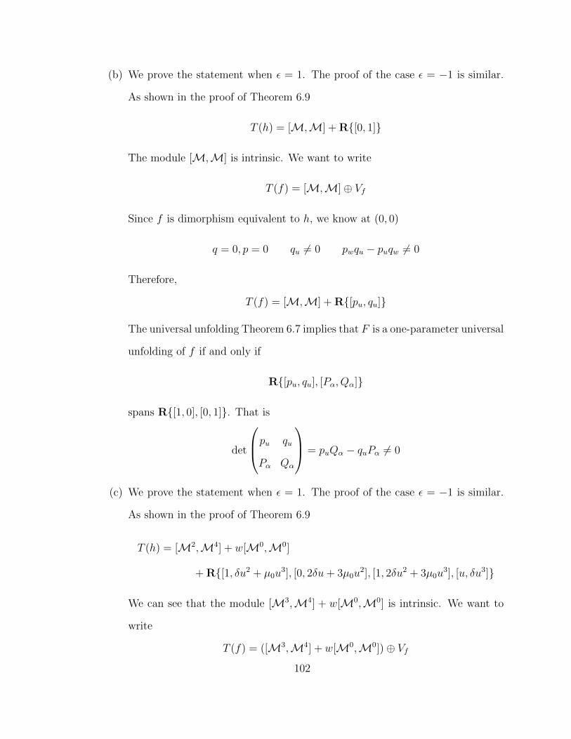
(b) We prove the statement when ε = 1. The proof of the case ε = −1 is similar.

As shown in the proof of Theorem 6.9

T (h) = [M,M] + R{[0, 1]}

The module [M,M] is intrinsic. We want to write

T (f) = [M,M]⊕ Vf

Since f is dimorphism equivalent to h, we know at (0, 0)

q = 0, p = 0 qu 6= 0 pwqu − puqw 6= 0

Therefore,

T (f) = [M,M] + R{[pu, qu]}

The universal unfolding Theorem 6.7 implies that F is a one-parameter universal

unfolding of f if and only if

R{[pu, qu], [Pα, Qα]}

spans R{[1, 0], [0, 1]}. That is

det

pu qu

Pα Qα

= puQα − quPα 6= 0

(c) We prove the statement when ε = 1. The proof of the case ε = −1 is similar.

As shown in the proof of Theorem 6.9

T (h) = [M2,M4] + w[M0,M0]

+ R{[1, δu2 + µ0u3], [0, 2δu+ 3µ0u

2], [1, 2δu2 + 3µ0u3], [u, δu3]}

We can see that the module [M3,M4] + w[M0,M0] is intrinsic. We want to

write

T (f) = ([M3,M4] + w[M0,M0])⊕ Vf102

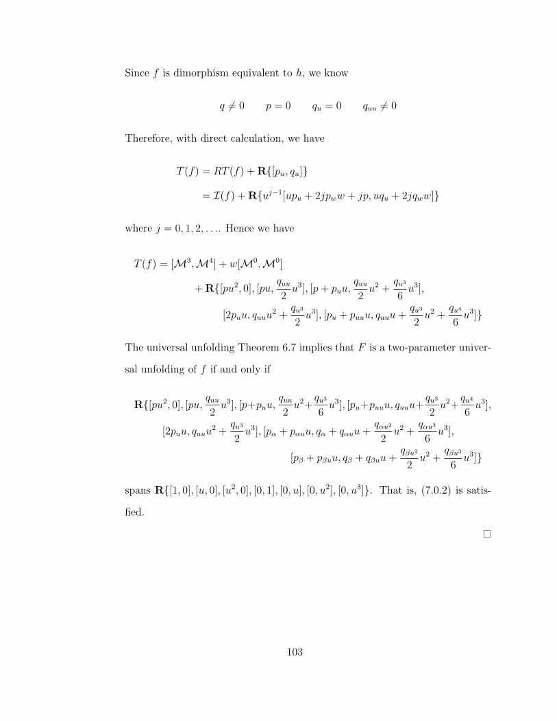
Since f is dimorphism equivalent to h, we know

q 6= 0 p = 0 qu = 0 quu 6= 0

Therefore, with direct calculation, we have

T (f) = RT (f) + R{[pu, qu]}

= I(f) + R{uj−1[upu + 2jpww + jp, uqu + 2jqww]}

where j = 0, 1, 2, . . .. Hence we have

T (f) = [M3,M4] + w[M0,M0]

+ R{[pu2, 0], [pu,quu2u3], [p+ puu,

quu2u2 +

qu3

6u3],

[2puu, quuu2 +

qu3

2u3], [pu + puuu, quuu+

qu3

2u2 +

qu4

6u3]}

The universal unfolding Theorem 6.7 implies that F is a two-parameter univer-

sal unfolding of f if and only if

R{[pu2, 0], [pu,quu2u3], [p+puu,

quu2u2+

qu3

6u3], [pu+puuu, quuu+

qu3

2u2+

qu4

6u3],

[2puu, quuu2 +

qu3

2u3], [pα + pαuu, qα + qαuu+

qαu2

2u2 +

qαu3

6u3],

[pβ + pβuu, qβ + qβuu+qβu2

2u2 +

qβu3

6u3]}

spans R{[1, 0], [u, 0], [u2, 0], [0, 1], [0, u], [0, u2], [0, u3]}. That is, (7.0.2) is satis-

fied.

103

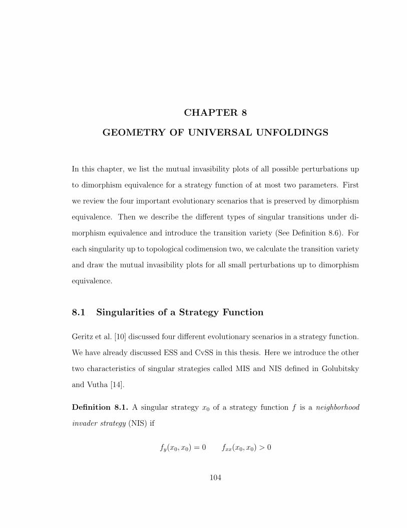
CHAPTER 8

GEOMETRY OF UNIVERSAL UNFOLDINGS

In this chapter, we list the mutual invasibility plots of all possible perturbations up

to dimorphism equivalence for a strategy function of at most two parameters. First

we review the four important evolutionary scenarios that is preserved by dimorphism

equivalence. Then we describe the different types of singular transitions under di-

morphism equivalence and introduce the transition variety (See Definition 8.6). For

each singularity up to topological codimension two, we calculate the transition variety

and draw the mutual invasibility plots for all small perturbations up to dimorphism

equivalence.

8.1 Singularities of a Strategy Function

Geritz et al. [10] discussed four different evolutionary scenarios in a strategy function.

We have already discussed ESS and CvSS in this thesis. Here we introduce the other

two characteristics of singular strategies called MIS and NIS defined in Golubitsky

and Vutha [14].

Definition 8.1. A singular strategy x0 of a strategy function f is a neighborhood

invader strategy (NIS) if

fy(x0, x0) = 0 fxx(x0, x0) > 0

104

Remark 8.2. The concept of NIS is first introduced by Apaloo [1]. If x0 is an NIS

of f , then x0 can always invade other local strategies when itself is initially rare.

Definition 8.3. A singular strategy x0 of a strategy function f is mutual invasibility

(MIS) if

fy(x0, x0) = 0 fyy(x0, x0) + fxx(x0, x0) > 0 (8.1.1)

Remark 1.10 shows that (8.1.1) is a sufficient condition for the existence of pairs

of dimorphisms around the singular strategy x0.

Dieckmann and Metz [4] discuss the evolutionary influence of these four types of

singular behaviors. These four singularities are summarized in Figure 8.1, which is a

modification of a picture in Geritz et al. [10]. This figure classifies the stabilities of

the singular strategies ESS, CvSS, NIS, and MIS.

Lemma 8.4. Dimorphism equivalence preserves the stabilities of ESS, CvSS, NIS,

and MIS for all strategy functions.

We recall that Golubitsky and Vutha [14] define

Definition 8.5. Two strategy functions f and f are strongly strategy equivalent if

f(x, y) = S(x, y)f(Φ(x, y))

where the following conditions are satisfied near a given point

1. S(x, y) > 0 for all x, y

2. Φ ≡ (Φ1,Φ2) where Φi: R2 → R, det(dΦ)x,y > 0 for all x, y

3. Φ1(x, x) = Φ2(x, x) for every x

4. (dΦ)x,x = α(x)I where α(x) > 0

105

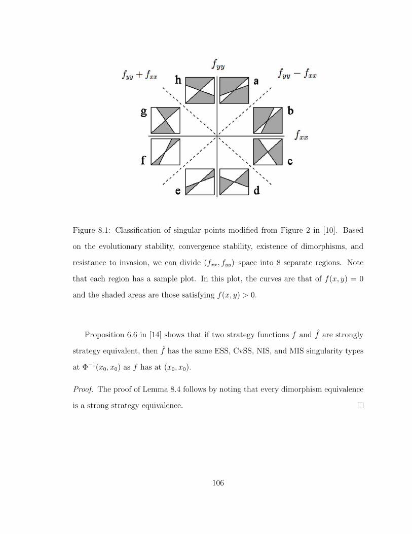
Figure 8.1: Classification of singular points modified from Figure 2 in [10]. Based

on the evolutionary stability, convergence stability, existence of dimorphisms, and

resistance to invasion, we can divide (fxx, fyy)–space into 8 separate regions. Note

that each region has a sample plot. In this plot, the curves are that of f(x, y) = 0

and the shaded areas are those satisfying f(x, y) > 0.

Proposition 6.6 in [14] shows that if two strategy functions f and f are strongly

strategy equivalent, then f has the same ESS, CvSS, NIS, and MIS singularity types

at Φ−1(x0, x0) as f has at (x0, x0).

Proof. The proof of Lemma 8.4 follows by noting that every dimorphism equivalence

is a strong strategy equivalence.

106

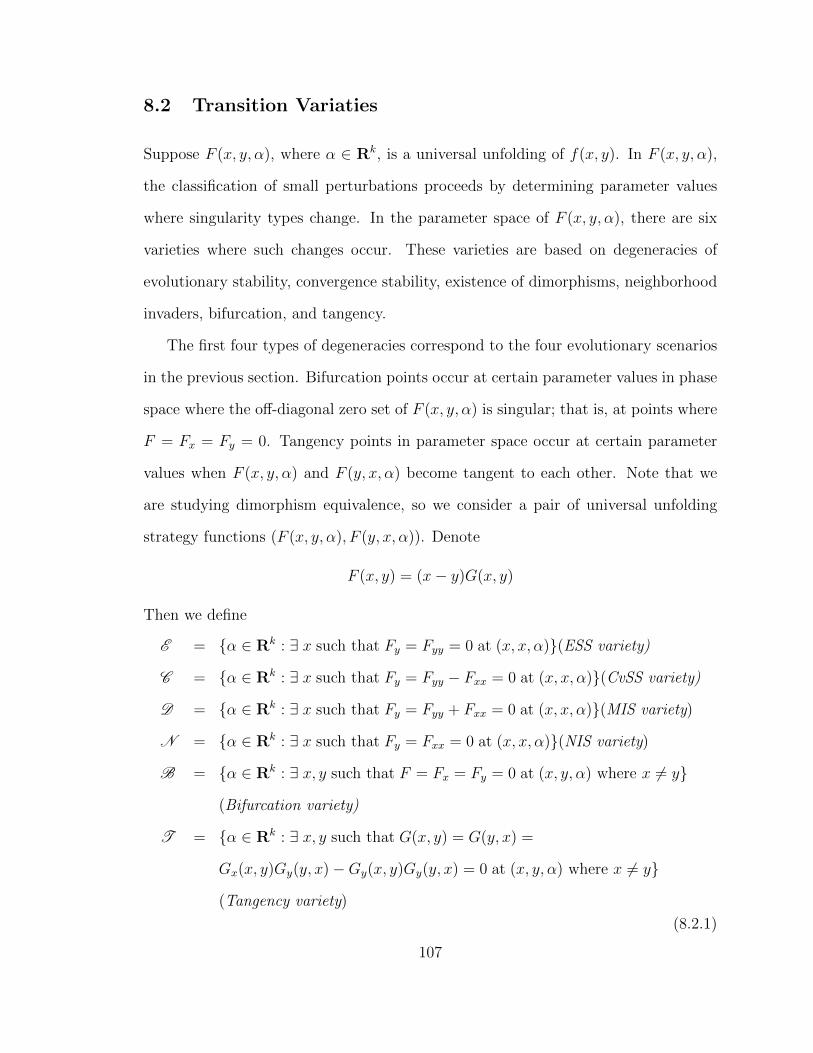
8.2 Transition Variaties

Suppose F (x, y, α), where α ∈ Rk, is a universal unfolding of f(x, y). In F (x, y, α),

the classification of small perturbations proceeds by determining parameter values

where singularity types change. In the parameter space of F (x, y, α), there are six

varieties where such changes occur. These varieties are based on degeneracies of

evolutionary stability, convergence stability, existence of dimorphisms, neighborhood

invaders, bifurcation, and tangency.

The first four types of degeneracies correspond to the four evolutionary scenarios

in the previous section. Bifurcation points occur at certain parameter values in phase

space where the off-diagonal zero set of F (x, y, α) is singular; that is, at points where

F = Fx = Fy = 0. Tangency points in parameter space occur at certain parameter

values when F (x, y, α) and F (y, x, α) become tangent to each other. Note that we

are studying dimorphism equivalence, so we consider a pair of universal unfolding

strategy functions (F (x, y, α), F (y, x, α)). Denote

F (x, y) = (x− y)G(x, y)

Then we define

E = {α ∈ Rk : ∃ x such that Fy = Fyy = 0 at (x, x, α)}(ESS variety)

C = {α ∈ Rk : ∃ x such that Fy = Fyy − Fxx = 0 at (x, x, α)}(CvSS variety)

D = {α ∈ Rk : ∃ x such that Fy = Fyy + Fxx = 0 at (x, x, α)}(MIS variety)

N = {α ∈ Rk : ∃ x such that Fy = Fxx = 0 at (x, x, α)}(NIS variety)

B = {α ∈ Rk : ∃ x, y such that F = Fx = Fy = 0 at (x, y, α) where x 6= y}

(Bifurcation variety)

T = {α ∈ Rk : ∃ x, y such that G(x, y) = G(y, x) =

Gx(x, y)Gy(y, x)−Gy(x, y)Gy(y, x) = 0 at (x, y, α) where x 6= y}

(Tangency variety)

(8.2.1)

107

Definition 8.6. The transition variety is the union of all the degenerate varieties in

(8.2.1). That is

T V = E ∪ C ∪D ∪N ∪B ∪T

We can simplify the calculation of transition varieties. Since the universal unfold-

ings of strategy functions vanish on the diagonal, we can define

F (x, y, α) = P (u,w, α)w +Q(u,w, α)v.

Therefore, with direct calculation, we obtain

E = {α ∈ Rk : ∃ u such that −Q = 2(P −Qu) = 0 at (u, 0, α)}

C = {α ∈ Rk : ∃ u such that −Q = −4Qu = 0 at (u, 0, α)}

D = {α ∈ Rk : ∃ u such that −Q = 4P = 0 at (u, 0, α)}

N = {α ∈ Rk : ∃ u such that −Q = 2(P +Qu) = 0 at (u, 0, α)}

B = {α ∈ Rk : ∃ u,w such that

Pv +Q = Puv +Qu = 2Pww + P + 2Qwv = 0 at (u, v, α) where v 6= 0}

T = {α ∈ Rk : ∃ u,w such that

Pv = Q = 2w(PuQw − PwQu)− PQu = 0 at (u, v, α) where v 6= 0}(8.2.2)

Remark 8.7. Note that we study ESS singularities, CvSS singularities, and dimor-

phisms in this thesis. We showed that dimorphism equivalence preserves these three

properties. In addition, we find that dimorphism equivalence preserves NIS as well.

Since Geritz et al. [10] point out that NIS is also one of the most important evolu-

tionary scenarios, we would like to consider the transition of stability of NIS as part

of the transition varieties too. That is, in the MIPs of the singularities, we identify

singularities with different stabilities of NIS as different singularities. This is just

something we have the option to keep track of along the way of drawing MIPs under

dimorphism equivalence.

108

8.3 Mutual Invasibility Plots

We classify persistent perturbations of low codimension singularities for strategy func-

tions and their universal unfoldings. A persistent perturbation is described by a

mutual invasibility plot.

Topological Codimension Zero.

(a) Theorem 6.9 shows that the universal unfolding of f = ε(w + µ0uv) is

F = ε(w + µuv)

where µ is a modal parameter near µ0 6= 0. Note that

P = ε Q = εµu

Therefore, the transition variety of F contains

E = {µ = ε} C = {µ = 0} D = ∅ N = {µ = −ε} B = ∅ T = ∅

The MIPs are displayed in Figure 2.1 and Figure 2.2 of Chapter 2. We see

that µ is a modal parameter. Thus, when µ0 6= ±1, 0 we have a topological

codimension zero singularity. However, the two special cases µ0 = ±1 generate

a topological codimension one singularity.

Topological Codimension One

(b) Theorem 6.9 shows that the universal unfolding of f = ε(δw2 + uv) is

F = ε((δw + a)w + uv)

where a is near 0. Note that

P = ε(δw + a) Q = εu

109

Therefore, the transition variety of F contains

E = ∅ C = ∅ D = {a = 0} N = ∅ B = ∅ T = ∅

The MIPs are displayed in Figure 2.3 of Chapter 2. Since we have one unfolding

parameter a, this is a topological codimension one singularity.

(c) Theorem 6.9 shows that the universal unfolding of f = (ε+ µ0u)w + δu2v is

F = (ε+ µu)w + (a+ δu2)v

Note that

P = ε+ µu Q = a+ δu2

Therefore, the transition variety of F contains

E = ∅ C = {a = 0} D = ∅ N = ∅ B = ∅ T = ∅

Figure 8.2 consists of MIPs of F for different µ, we can see that values of µ do not

change the existence of dimorphisms and the stabilities of singularities. Even

though strategy functions with distinct µ values are not dimorphism equivalent,

we still have an intuitive idea that the MIPs with different µ share the same

singular and dimorphism properties. In particular, the MIPs when µ = 0 are

displayed in Figure 2.4 of Chapter 2. Since µ is a modal parameter and a is an

unfolding parameter, we have a topological codimension one singularity.

110

+−

+−

−+

−+

−−

−−−−

−−

+−

−+

+−

−+

+−

−+

−−

−+

+−

−−

−+

+−

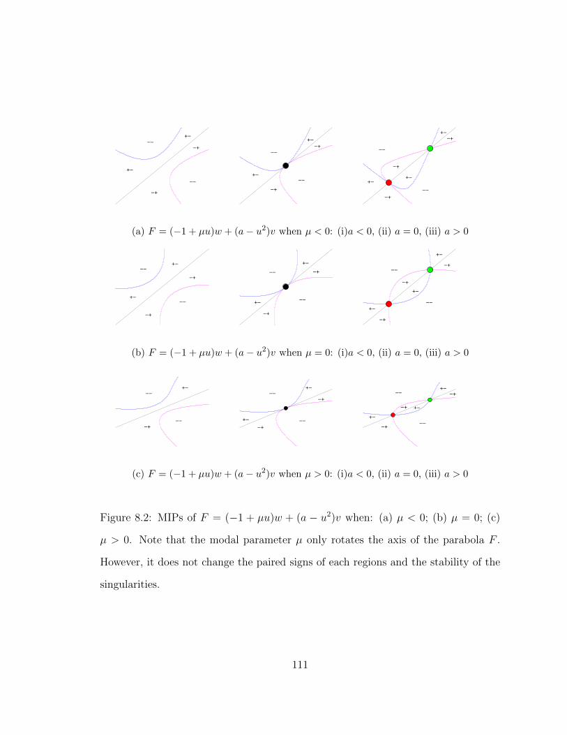
(a) F = (−1 + µu)w + (a− u2)v when µ < 0: (i)a < 0, (ii) a = 0, (iii) a > 0

−−

+−

−+

+−

−+

−−

−−

−−+−

−+

+−

−+

+−

−+

−+

+−

+−

−+

−−

−−

(b) F = (−1 + µu)w + (a− u2)v when µ = 0: (i)a < 0, (ii) a = 0, (iii) a > 0

+−

−+

−−

−− +−

+−

−+

−+

−−

−−

−−

−−

+−

−+

−+

+−

−+ +−

(c) F = (−1 + µu)w + (a− u2)v when µ > 0: (i)a < 0, (ii) a = 0, (iii) a > 0

Figure 8.2: MIPs of F = (−1 + µu)w + (a − u2)v when: (a) µ < 0; (b) µ = 0; (c)

µ > 0. Note that the modal parameter µ only rotates the axis of the parabola F .

However, it does not change the paired signs of each regions and the stability of the

singularities.

111

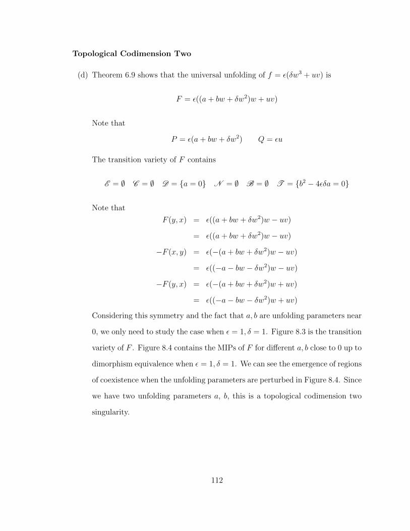
Topological Codimension Two

(d) Theorem 6.9 shows that the universal unfolding of f = ε(δw3 + uv) is

F = ε((a+ bw + δw2)w + uv)

Note that

P = ε(a+ bw + δw2) Q = εu

The transition variety of F contains

E = ∅ C = ∅ D = {a = 0} N = ∅ B = ∅ T = {b2 − 4εδa = 0}

Note that

F (y, x) = ε((a+ bw + δw2)w − uv)

= ε((a+ bw + δw2)w − uv)

−F (x, y) = ε(−(a+ bw + δw2)w − uv)

= ε((−a− bw − δw2)w − uv)

−F (y, x) = ε(−(a+ bw + δw2)w + uv)

= ε((−a− bw − δw2)w + uv)

Considering this symmetry and the fact that a, b are unfolding parameters near

0, we only need to study the case when ε = 1, δ = 1. Figure 8.3 is the transition

variety of F . Figure 8.4 contains the MIPs of F for different a, b close to 0 up to

dimorphism equivalence when ε = 1, δ = 1. We can see the emergence of regions

of coexistence when the unfolding parameters are perturbed in Figure 8.4. Since

we have two unfolding parameters a, b, this is a topological codimension two

singularity.

112

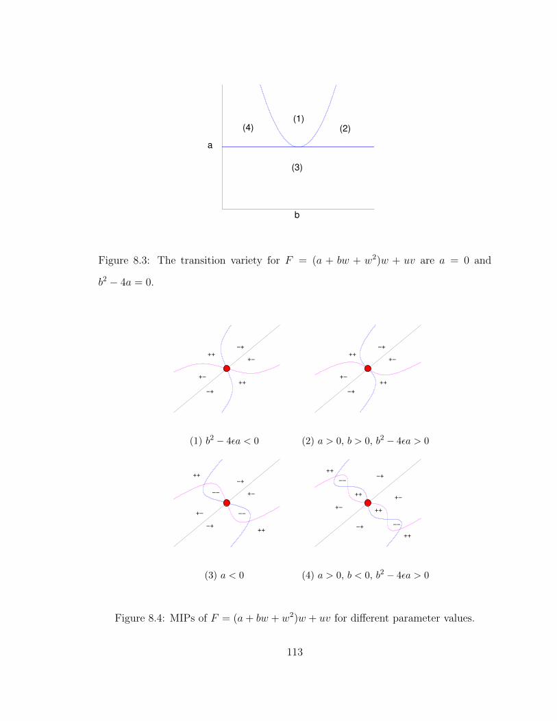
b

a

(1)

(3)

(4) (2)

Figure 8.3: The transition variety for F = (a + bw + w2)w + uv are a = 0 and

b2 − 4a = 0.

++

++

−+

−+

+−

+−

(1) b2 − 4εa < 0

++

++

−+

−+

+−

+−

(2) a > 0, b > 0, b2 − 4εa > 0

+−−−

−−

−+

−+

++

++

+−

(3) a < 0

−+

+−

−+

+−

−−

−−

++

++

++

++

(4) a > 0, b < 0, b2 − 4εa > 0

Figure 8.4: MIPs of F = (a+ bw + w2)w + uv for different parameter values.

113

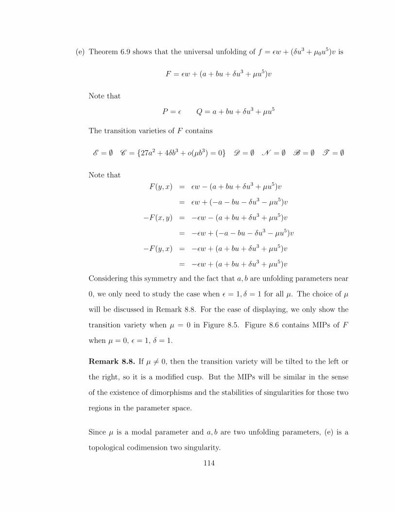
(e) Theorem 6.9 shows that the universal unfolding of f = εw + (δu3 + µ0u5)v is

F = εw + (a+ bu+ δu3 + µu5)v

Note that

P = ε Q = a+ bu+ δu3 + µu5

The transition varieties of F contains

E = ∅ C = {27a2 + 4δb3 + o(µb3) = 0} D = ∅ N = ∅ B = ∅ T = ∅

Note that

F (y, x) = εw − (a+ bu+ δu3 + µu5)v

= εw + (−a− bu− δu3 − µu5)v

−F (x, y) = −εw − (a+ bu+ δu3 + µu5)v

= −εw + (−a− bu− δu3 − µu5)v

−F (y, x) = −εw + (a+ bu+ δu3 + µu5)v

= −εw + (a+ bu+ δu3 + µu5)v

Considering this symmetry and the fact that a, b are unfolding parameters near

0, we only need to study the case when ε = 1, δ = 1 for all µ. The choice of µ

will be discussed in Remark 8.8. For the ease of displaying, we only show the

transition variety when µ = 0 in Figure 8.5. Figure 8.6 contains MIPs of F

when µ = 0, ε = 1, δ = 1.

Remark 8.8. If µ 6= 0, then the transition variety will be tilted to the left or

the right, so it is a modified cusp. But the MIPs will be similar in the sense

of the existence of dimorphisms and the stabilities of singularities for those two

regions in the parameter space.

Since µ is a modal parameter and a, b are two unfolding parameters, (e) is a

topological codimension two singularity.

114

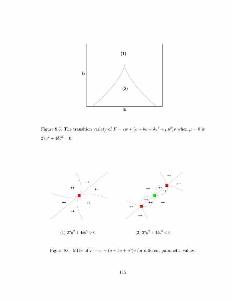
a

b

(1)

(2)

Figure 8.5: The transition variety of F = εw + (a + bu + δu3 + µu5)v when µ = 0 is

27a2 + 4δb3 = 0.

−+

+−++

+++−

−+

(1) 27a2 + 4δb3 > 0

−+

+−

−+

+−

+−

−+

+−

−+

++

++

(2) 27a2 + 4δb3 < 0

Figure 8.6: MIPs of F = w + (a+ bu+ u3)v for different parameter values.

115

(f) Theorem 6.9 shows that the universal unfolding of f = ε(uw + (α0w + β0u2)v)

is

F = ε((a+ u)w + (b+ αw + βu2)v)

where a, b are unfolding parameters near 0 and α, β are modal parameter near

α0, β0. Note that

P = ε(a+ u) Q = ε(b+ αw + βu2)

The transition variety of F contains

E = {εa2β + b(1− 2β)2 = 0} C = {b = 0}

D = {εa2β + b = 0} N = {εa2β + b(1 + 2β)2 = 0}

B = {εa2β − b(4αβ − 1) = 0} T = {α = 0}

Note that in Theorem 6.9 we have assumptions

α 6= 0 β 6= 0 4αβ − 1 6= 0

So we know

T = ∅

From the definition of the varieties, we see a few degeneracies of the transition

variety when modal parameter α, β are varied. In summary, we have

(i) If β = ±1

2, E or N would degenerate from parabola to a straight line;

(ii) If β = ±1, E or N would overlap with D ;

(iii) If α + β = ±1, , E or N would overlap with B.

In addition, under the symmetry σ(x, y) = (y, x) we have

F (y, x) = ε((a+ u)w − (b+ αw + βu2)v)

= ε((a+ εu)w + (−b− αw − βu2)v)

116

Moreover,

−F (x, y) = ε(−(a+ u)w − (b+ αw + βu2)v)

= ε((−a− εu)w + (−b− αw − βu2)v)

So we know

−F (y, x) = ε(−(a+ u)w + (b+ αw + βu2)v)

= ε((−a− εu)w + (b+ αw + βu2)v)

Considering that a, b are unfolding parameters near 0, we only need to study

the perturbation of f = ε(uw + (α0w + β0u2)v) when ε = 1, α0 > 0 since the

other 3 cases can be obtained through symmetries. In addition, if we assume

ε = 1, α0 > 0, then the universal unfolding becomes

F = (a+ u)w + (b+ αw + βu2)v

where α > 0. Note that when ε = 1, α > 0, we see

−F (−x,−y) = ε(−(a− u)w + (b+ αw + βu2)v)

= ε((−a+ u)w + (b+ αw + βu2)v)(8.3.1)

Since a, b are unfolding parameters close to 0, Equation (8.3.1) indicates that a

special symmetry exists when we change the parameter from a to −a.

Next, we work on the transition variety and MIPs of the universal unfolding

F = ε((a+ u)w + (b+ αw + βu2)v) for different parameter values.

First we divide the modal parameter space (α, β) into regions with the same

transition variety. Figure 8.7 is the separation of the modal parameters space.

Second, we look at the transition variety F for different a, b close to 0 when

ε = 1, α > 0. Figure 8.8 is the transition variety plot (respective to unfolding

parameter a, b) for each numbered region in Figure 8.7.

117

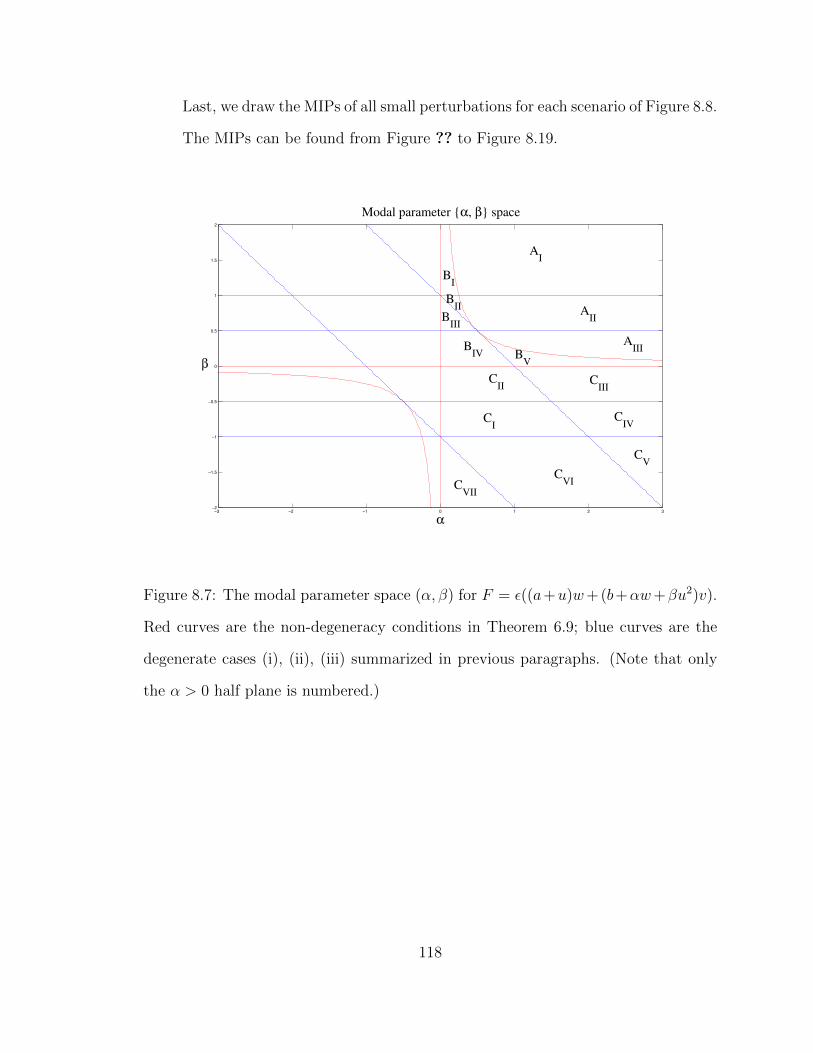
Last, we draw the MIPs of all small perturbations for each scenario of Figure 8.8.

The MIPs can be found from Figure ?? to Figure 8.19.

α

β

Modal parameter {α, β} space

−3 −2 −1 0 1 2 3

−2

−1.5

−1

−0.5

0

0.5

1

1.5

2

AI

AIIIB

IV

CI

CII

CIII

CIV

CV

CVIC

VII

BI

BV

AII

BII

BIII

Figure 8.7: The modal parameter space (α, β) for F = ε((a+u)w+ (b+αw+βu2)v).

Red curves are the non-degeneracy conditions in Theorem 6.9; blue curves are the

degenerate cases (i), (ii), (iii) summarized in previous paragraphs. (Note that only

the α > 0 half plane is numbered.)

118

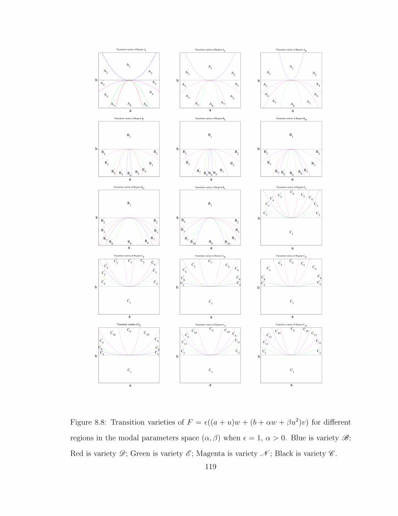
a

b

Transition variety of Region AI

A1

A2

A3

A4

A5

A2

’

A3

’

A4

’

A5

’ A6

a

b

Transition variety of Region AII

A1

A2

A3

A4

A6

A2

’

A3

’

A4

’

A7

’ A7

a

b

Transition variety of Region AIII

A1

A2

’

A3

’ A3

A2

A4

’A

4

A7

A7

’

A8

a

b

Transition variety of Region BI

B1

B6

B5

B4

B3

B2

B5

’B4

’

B3

’

B2

’

a

b

Transition variety of Region BII

B1

B2

’

B3

’B

3

B2

B5

B6

B5

’B7

’ B7

a

b

Transition variety of Region BIII

B1

B2

’

B3

’B

3

B2

B7

’ B7B

8B8

’B

6

a

b

Transition variety of Region BIV

B1

B2

B2

’

B7

B3

’

B7

’

B8

’ B8

B3

B9

a

b

Transition variety of Region BV

B7

’

B9

B2

B1

B2

’

B3

’B

3

B10

B7

B10

’

a

b

Transition variety of Region CI

C6

C2

’

C4

’C

5

’

C2

C3

’C

3

C4

C5

C1

a

b

Transition variety of Region CII

C2

’C

2

C1

C3

C4

C5

C3

’

C4

’C

5

’ C7

a

b

Transition variety of Resion CIII

C2

’ C2

C8

’ C8

C4C

4

’

C5

’C

5

C7

C1

a

b

Transition variety of Region CIV

C1

C9

C8

’

C4

’

C5

’C

5C

4

C8

C2C

2

’

a

b

Transition variety of CV

C1

C9

C4C

4

’

C10

’

C8

C2

C2

’

C8

’

C10

a

b

Transition variety of Region CVI

C1

C2

C2

’

C10

’

C11

C4

’

C11

’

C9 C

10C

4

a

b

Transition variety of Region CVII

C1

C2

’

C11

’

C9

C2

C12

’C

10

’

C11

C10

C12

Figure 8.8: Transition varieties of F = ε((a + u)w + (b + αw + βu2)v) for different

regions in the modal parameters space (α, β) when ε = 1, α > 0. Blue is variety B;

Red is variety D ; Green is variety E ; Magenta is variety N ; Black is variety C .

119

−+

+−

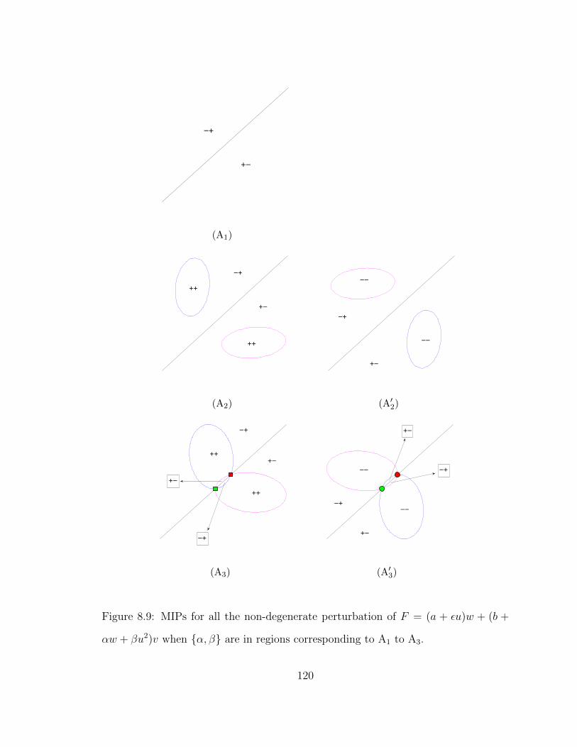
(A1)

++

++

−+

+−

(A2)

−−

−−

−+

+−

(A′2)

++

−+

+−

++

+−

−+

(A3)

−−

−−

+−

−+

+−

−+

(A′3)

Figure 8.9: MIPs for all the non-degenerate perturbation of F = (a + εu)w + (b +

αw + βu2)v when {α, β} are in regions corresponding to A1 to A3.

120

++

++

+−

−+

+−

−+

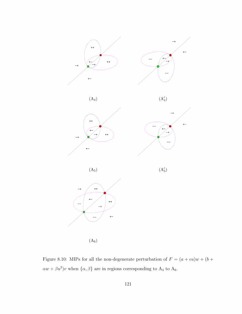
(A4)

−+

−−

−−

+−

−+

+−

(A′4)

+−

−+ ++

++

−+

+−

(A5)

−−

−−

+−

−+

−+

+−

(A′5)

++

+−

−+

++

−−

−− +−

−+

(A6)

Figure 8.10: MIPs for all the non-degenerate perturbation of F = (a + εu)w + (b +

αw + βu2)v when {α, β} are in regions corresponding to A4 to A6.

121

++

++

+−

−+

−−

−−

−+

+−

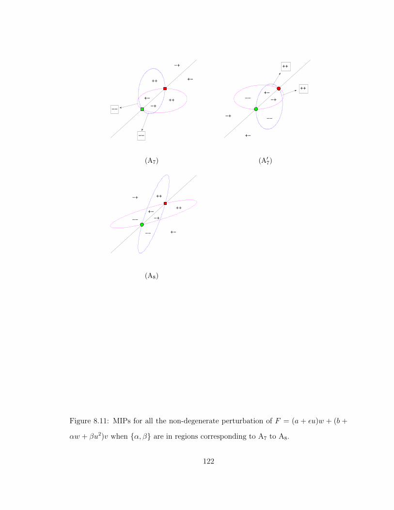
(A7)

+−

−+

−−

−−

++

++

−+

+−

(A′7)

++

+−

−+

−−

−−

++−+

+−

(A8)

Figure 8.11: MIPs for all the non-degenerate perturbation of F = (a + εu)w + (b +

αw + βu2)v when {α, β} are in regions corresponding to A7 to A8.

122

++

++

−−

−−

−+

+−

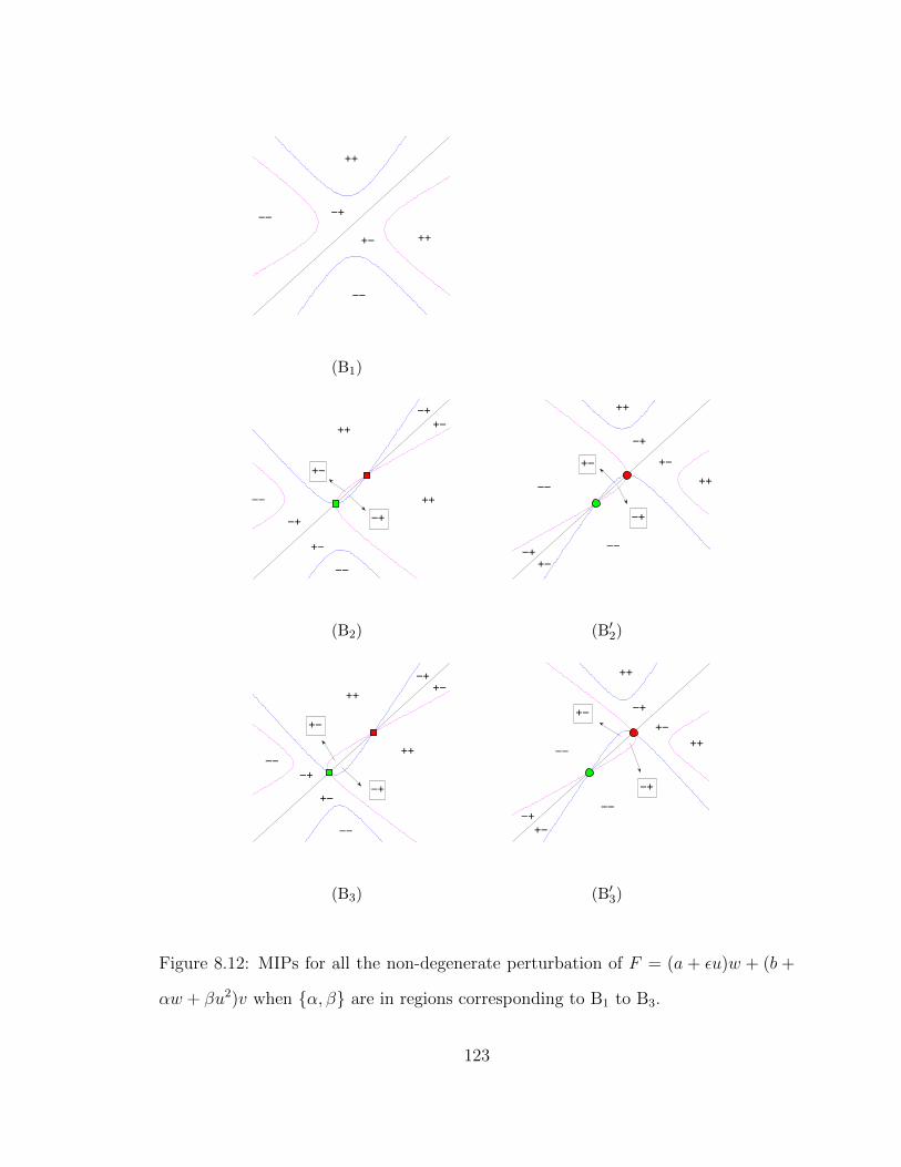
(B1)

+−

−+

−−

−+

−−

−+

+−

++

++

+−

(B2)

++

−+

+−

−+

−−

−+

+−

++

−−

+−

(B′2)

+−

+−

++

−+

++

+−

−+

−−

−−

−+

(B3)

++

−+

+−

++

−+

−−

+−

−−

−+

+−

(B′3)

Figure 8.12: MIPs for all the non-degenerate perturbation of F = (a + εu)w + (b +

αw + βu2)v when {α, β} are in regions corresponding to B1 to B3.

123

−−

−−

+−

−+

+−

−+

++

++−+

+−

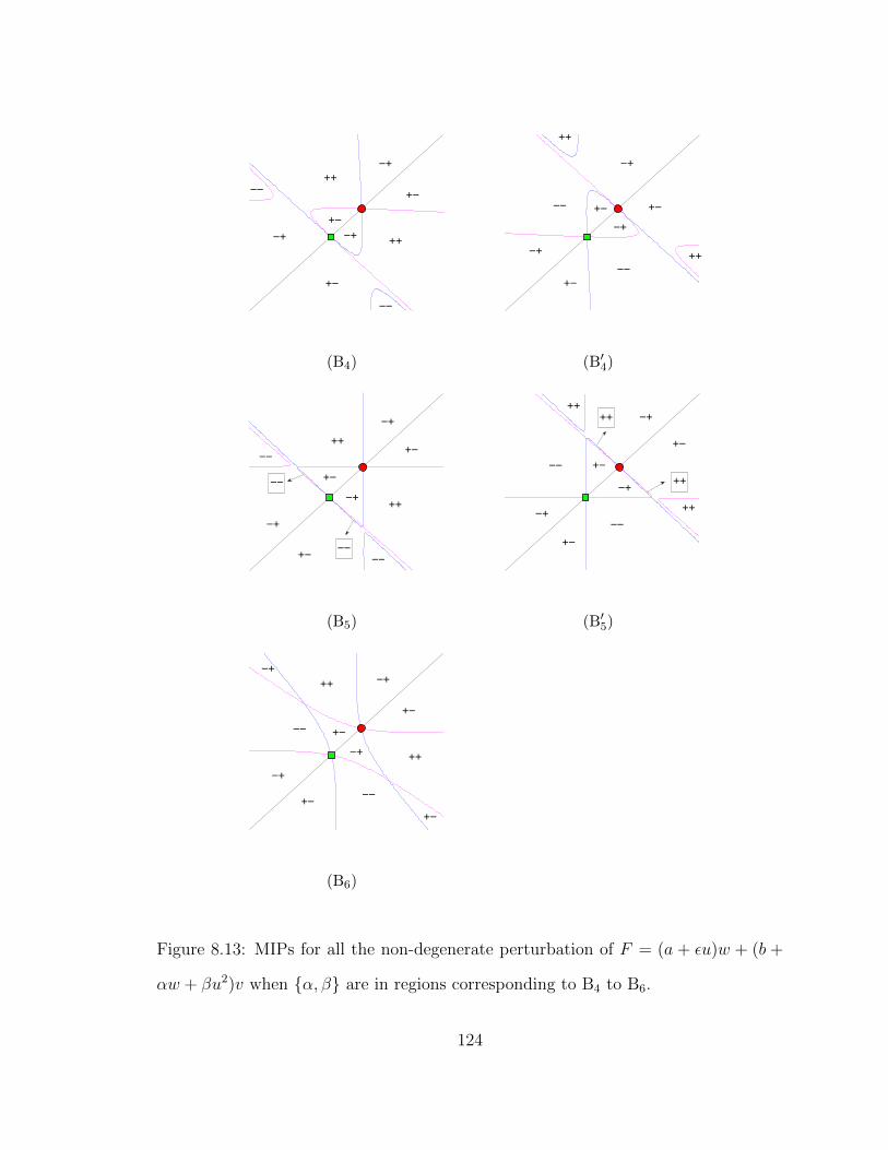
(B4)

++

−+

+−

++

−−

−−

−+

+−

−+

+−

(B′4)

+−

−+

++

−+

+−

−−

−−

−+

−−+−

−−

++

(B5)

++

++

++ −+

−+

+−−−

−−

+−

−+++

+−

(B′5)

+−

−+

−+

−+

+−

−−

−−

++−+

+−

++

+−

(B6)

Figure 8.13: MIPs for all the non-degenerate perturbation of F = (a + εu)w + (b +

αw + βu2)v when {α, β} are in regions corresponding to B4 to B6.

124

+−

−−

++

−+

++

+−

−+

−+

+−

−−

−−

−−

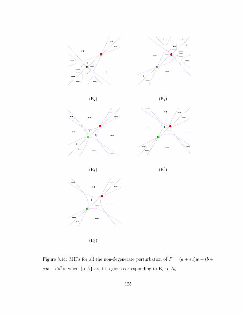
(B7)

++

++

++

−+

+−−−

−−

−+

+−

++ −+

+−

(B′7)

+−

−+

+−

−+

−+

+−

−−

−+

+−

++

−−

++

(B8)

−+

+−

++

+−

−+

+−

++

−+

−−

−+

+−

−−

(B′8)

−+

+−

+−

−+

+−

−+

−+

+−

−−

−−

++

++

(B9)

Figure 8.14: MIPs for all the non-degenerate perturbation of F = (a + εu)w + (b +

αw + βu2)v when {α, β} are in regions corresponding to B7 to A9.

125

−−

−−

−−

+−

−+

+−

++

++

+−

−+

−+

−−

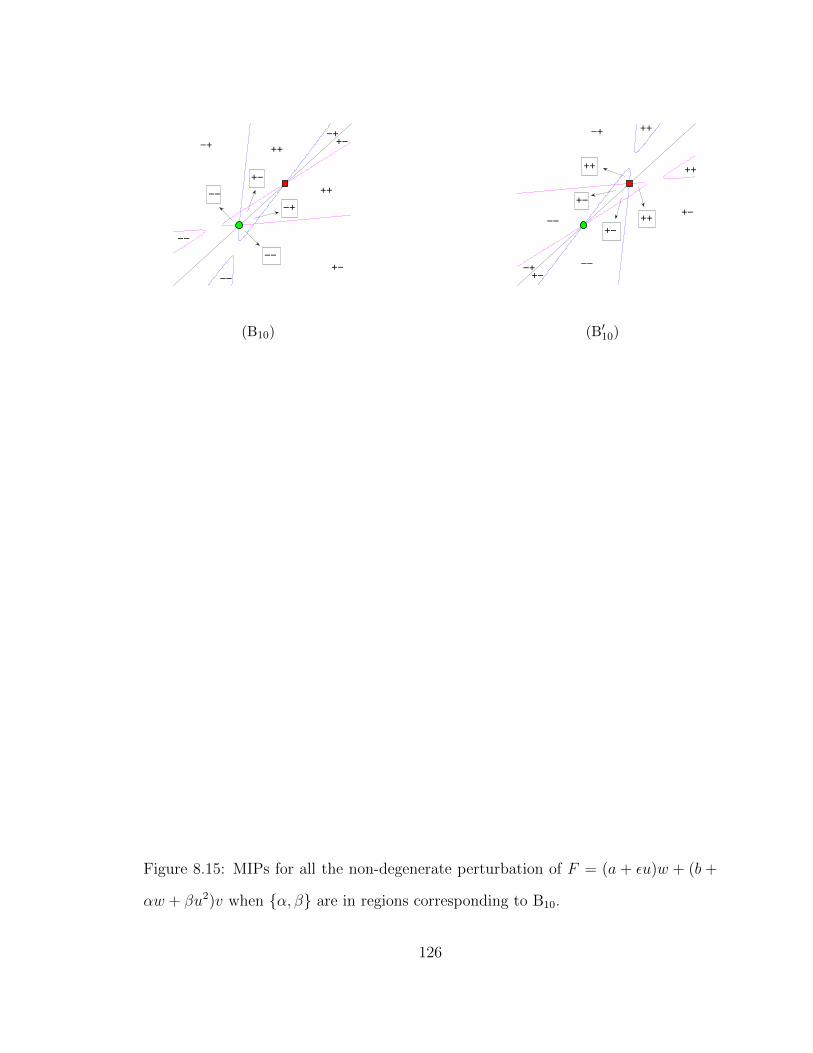
(B10)

++

++

++

+−

−+++

+−

+−

−−

−−

−+

+−

(B′10)

Figure 8.15: MIPs for all the non-degenerate perturbation of F = (a + εu)w + (b +

αw + βu2)v when {α, β} are in regions corresponding to B10.

126

++

−+

−−+−

++

+−

−−

−+

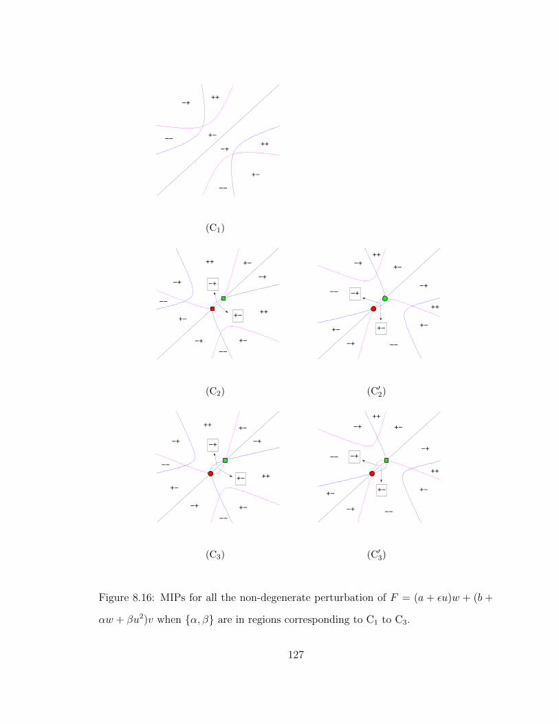
(C1)

−−

+−

−+

+−++

++

−+

−−

+−

−+

−+

+−

(C2)

++

+−

++

−+

+−−+

−+

+−

−−

−−

−+

+−

(C′2)

+−

−+−+

−−

+−

−+

−−

+−

−+

+−++

++

(C3)

++

++

+−+−

−+

−+

−+

+−

−−

−−

−+

+−

(C′3)

Figure 8.16: MIPs for all the non-degenerate perturbation of F = (a + εu)w + (b +

αw + βu2)v when {α, β} are in regions corresponding to C1 to C3.

127

++

−+

+−++

++

−+

−−

+−

−+

−−

++ +−

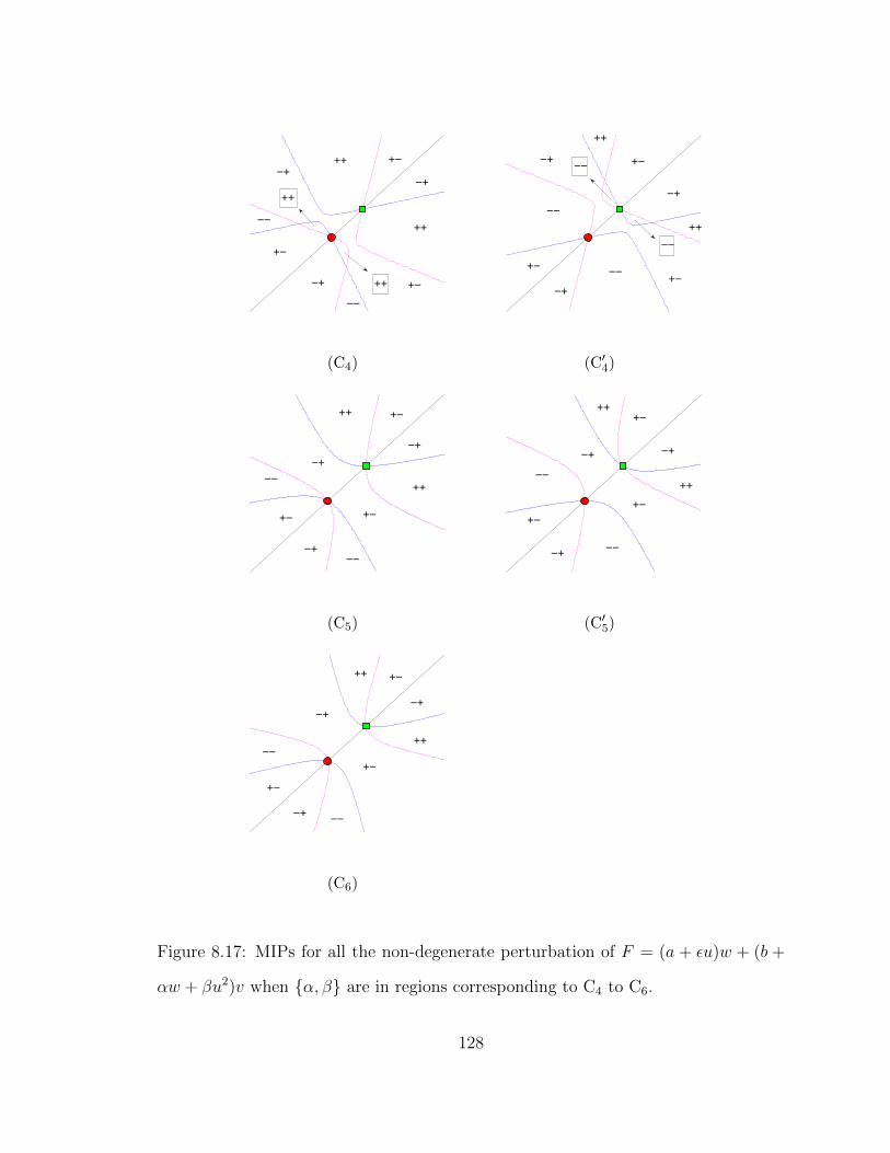
(C4)

−+

−−

−−

+−

−+

−−

+−−−

++

+−

++

−+

(C′4)

−−

−+

+−

−−

−+

+−

++

++ +−

−+

(C5)

++

+−

−+

++

+−

−+

−+

+−

−−

−−

(C′5)

+−

−+

+++−

−+

++

+−

−+

−−

−−

(C6)

Figure 8.17: MIPs for all the non-degenerate perturbation of F = (a + εu)w + (b +

αw + βu2)v when {α, β} are in regions corresponding to C4 to C6.

128

+−

−+

++

++

−+

+−

−−

+−

−+ −−

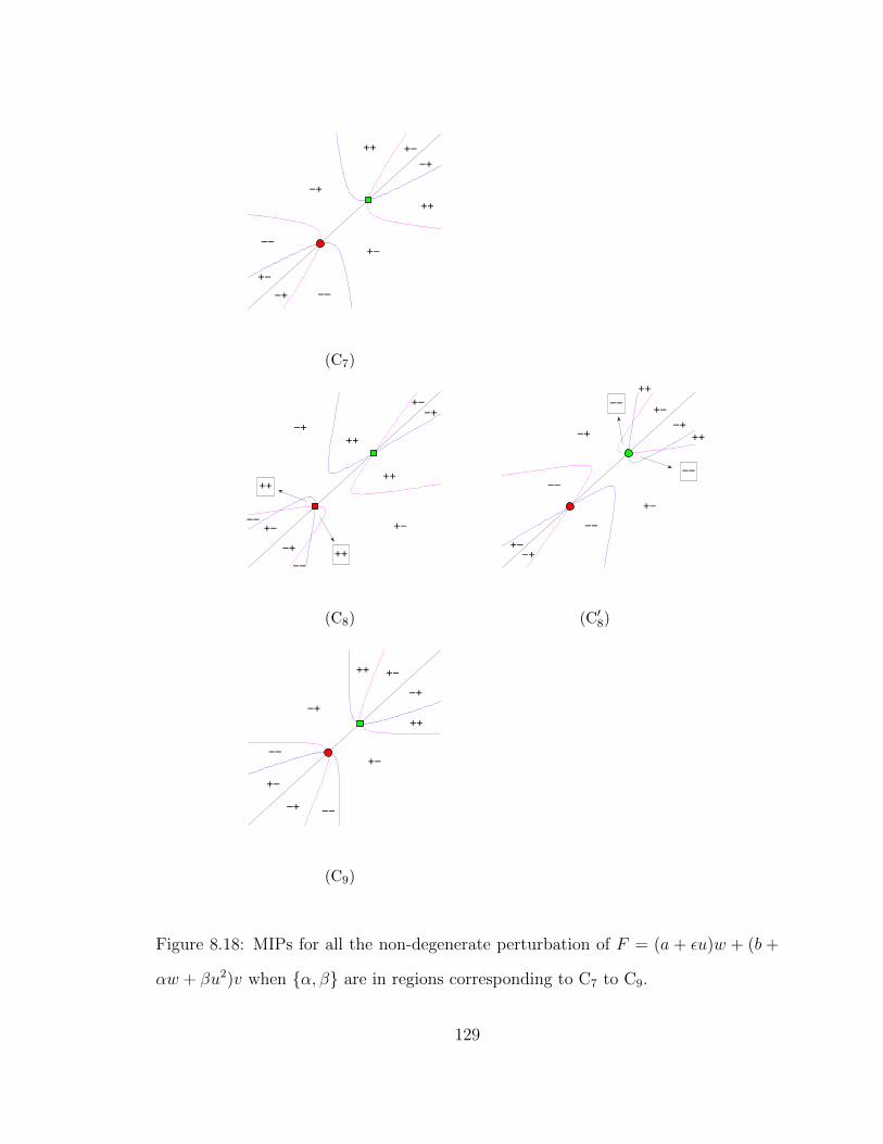
(C7)

−−

+−

−+

+−

++

++

+−

−+

−+

−−

++

++

(C8)

++

−+

+−

+−

−+

−−

−−

−+

++

+−

−−

−−

(C′8)

+++−

−+

++

−+

+−

−−

−−

+−

−+

(C9)

Figure 8.18: MIPs for all the non-degenerate perturbation of F = (a + εu)w + (b +

αw + βu2)v when {α, β} are in regions corresponding to C7 to C9.

129

−−

−−

−+

+−

++

++

−+

+−

++

++ +−

−+

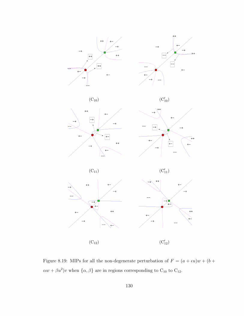
(C10)

−+

+−

−−

−−

−−

−−

+−

−+

++

++

−+

+−

(C′10)

−+

+−

−−

+−

++

+−

−+

−+

+−

++

−+

−−

(C11)

−+−−

++

+− +−

++

+−

−+

−−

+−

−+

−+

(C′11)

+−

−+

−+

+−

++

−−

+−

−+

++

−−

−+

+−

(C12)

+−

−+

−+

+−

++−+

++

+−

−−

−−

−+

+−

(C′12)

Figure 8.19: MIPs for all the non-degenerate perturbation of F = (a + εu)w + (b +

αw + βu2)v when {α, β} are in regions corresponding to C10 to C12.

130

BIBLIOGRAPHY

[1] J. Apaloo. Revisiting strategic models of evolution: the concept of neighborhoodinvader strategies. Theor. Pop. Biol. 52 (1997) 71–77.

[2] J. Damon. The unfolding and determinacy theorems for subgroups A and K.Memoirs of the American Mathematical Society 306, 1984.

[3] F. Dercole and S. Rinaldi. Analysis of evolutionary processes, The adaptivedynamics approach and its applications. Princeton University Press, Princeton,2008.

[4] U. Dieckmann, M. Doebeli, J.A.J. Metz, and D. Tautz. Adaptive speciation.Cambridge Studies in Adaptive Dynamics, 2004.

[5] U. Dieckmann and R. Law. The dynamical theory of coevolution: a derivationfrom stochastic ecological processes. Journal of Mathematical Biology 34 (1996)569–612.

[6] U. Dieckmann and J.A.J. Metz. Surprising evolutionary predictions from en-hanced ecological realism. Theoretical Population Biology 69 (2006) 263–281.

[7] O. Diekmann. A beginner’s guide to adaptive dynamics. Banach Center Publ.63 (2003) 47–86.

[8] S.A.H. Geritz and E. Kisdi. Adaptive dynamics in diploid, sexual populationsand the evolution of reproductive isolation. Proc. R. Soc. Lond. Ser. B-Biol.Sci. 267 (2000) 1671–1678.

[9] S. A. H. Geritz, E. Kisdi, G. Meszena, and J. A. J. Metz. Evolutionarily singularstrategies and the adaptive growth and branching of the evolutionary tree. Evol.Ecol. 12 (1998) 35–57.

[10] S.A.H. Geritz, J.A.J. Metz, E. Kisdi, and G. Meszena. Dynamics of adaptationand evolutionary branching. Physical Review Letters 78 (1997) 2024–2027.

[11] M. Golubitsky and V. Guillemin. Stable Mappings and Their Singularities, GTM14, Springer-Verlag, New York, 1974

131

[12] M. Golubitsky and D.G. Schaeffer. Singularities and Groups in Bifurcation The-ory: Vol 1. Applied Mathematical Sciences 51, Springer, 1985.

[13] M. Golubitsky and D.G. Schaeffer. Singularities and Groups in Bifurcation The-ory: Vol 2. Applied Mathematical Sciences 69, Springer, 1988.

[14] M. Golubitsky and A. Vutha. Normal forms and unfoldings of singular strategyfunctions. Dynam. Games Appl (2014) DOI 10.1007/s13235-014-0116-0.

[15] H. C. Ito and U. Dieckmann. Evolutionary-branching lines and areas in bivariatetrait spaces. Evolutionary Ecology Research 14 (2012) 555–582.

[16] E. Kisdi and T. Priklopil. Evolutionary branching of a magic trait. J. Math.Biol. 63 (2011) 36–397.

[17] J. Maynard-Smith and G. R. Price. The logic of animal conflict. Nature 246(1973) 15–18.

[18] J. Polechova and N. H. Barton. Speciation through competition: A criticalreview. Evolution 59 (2005) 1194–1210.

[19] D. Waxman and S. Gavrilets. 20 questions on adaptive dynamics. Journal ofEvolutionary Biology 18 (5) (2005) 1139–1154.

132