


![Structure from Motion Summaryicarus.csd.auth.gr/wp-content/uploads/2020/05/... · [15] David Tschumperle and Rachid Deriche, ^Vector-valued image regularization with pdes: A common](https://static.fdocuments.net/doc/165x107/602b641d8987a875e9333883/structure-from-motion-15-david-tschumperle-and-rachid-deriche-vector-valued.jpg)

Languages
Pages
Legal


Singapore
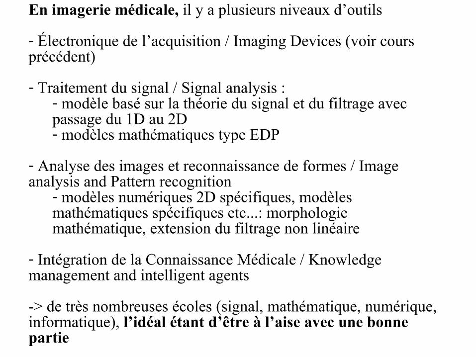
En imagerie médicale, il y a plusieurs niveaux d’outils
- Électronique de l’acquisition / Imaging Devices (voir cours précédent)
- Traitement du signal / Signal analysis : - modèle basé sur la théorie du signal et du filtrage avec passage du 1D au 2D- modèles mathématiques type EDP
- Analyse des images et reconnaissance de formes / Image analysis and Pattern recognition
- modèles numériques 2D spécifiques, modèles mathématiques spécifiques etc...: morphologie mathématique, extension du filtrage non linéaire
- Intégration de la Connaissance Médicale / Knowledge management and intelligent agents
-> de très nombreuses écoles (signal, mathématique, numérique, informatique), l’idéal étant d’être à l’aise avec une bonne partie
Problématiques actuelles
Singapore
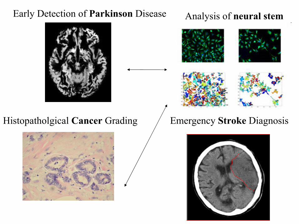
Emergency Stroke DiagnosisHistopatholgical Cancer Grading
Early Detection of Parkinson Disease Analysis of neural stem
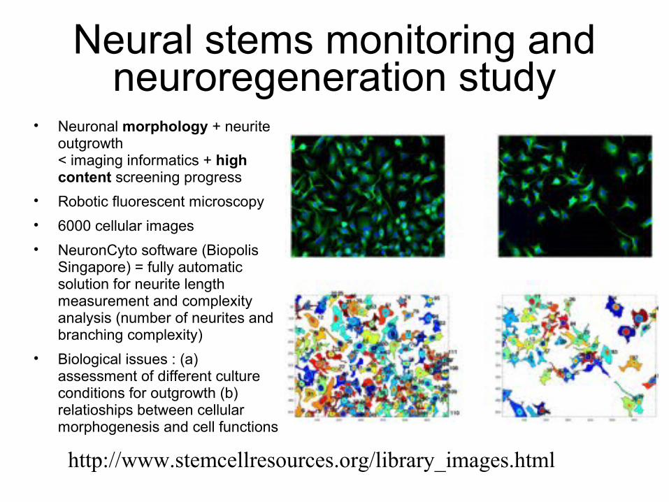
Neural stems monitoring and neuroregeneration study
• Neuronal morphology + neurite outgrowth < imaging informatics + high content screening progress
• Robotic fluorescent microscopy
• 6000 cellular images
• NeuronCyto software (Biopolis Singapore) = fully automatic solution for neurite length measurement and complexity analysis (number of neurites and branching complexity)
• Biological issues : (a) assessment of different culture conditions for outgrowth (b) relatioships between cellular morphogenesis and cell functions
http://www.stemcellresources.org/library_images.html

Estelle Glory
Acquisition and processing of
colored cultured cells
Related Past
Projects

Acquisition System :inverted, motorized microscope with computer control
1
Inverted microscope•objectifs x10, x20 •motorized stage (x,y) •motorized z (focus)•fluorescence possible adaptation
Computer + software•control of plate moving•autofocus•control of camera acquisition•image storage
Digital camera•color•cooled•…
Related Past
Projects

•magenta-colored nuclei → green component•grey level threshold•size selection
Image processing : segmentation of nuclei
2
1. Thresholding
Original image Green component of rgb
Isolated nuclei
Adjacent nuclei
Automatic threshold (iterative)
Related Past
Projects
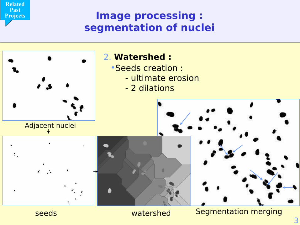
•Seeds creation : - ultimate erosion- 2 dilations
Image processing :segmentation of nuclei
3
2. Watershed :
seeds watershed Segmentation merging
Adjacent nuclei
Related Past
Projects
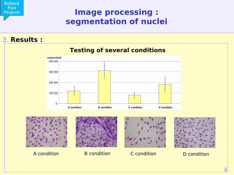
3. Results :
4
Testing of several conditions
B condition C condition D condition
0
100 000
200 000
300 000
400 000
A condition B condition C condition D condition
noyaux/puits
A condition
Image processing :segmentation of nuclei
Related Past
Projects
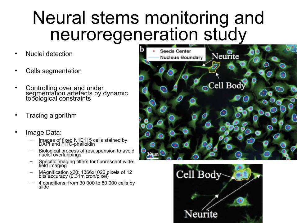
Neural stems monitoring and neuroregeneration study
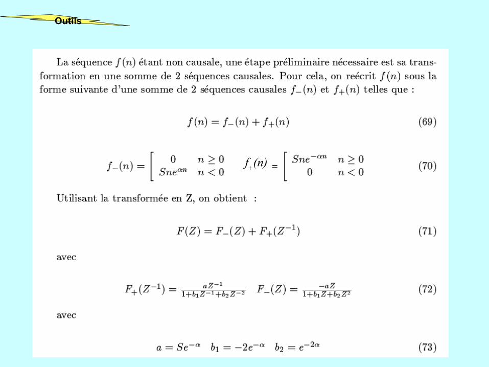
• Nuclei detection
• Cells segmentation
• Controlling over and under segmentation artefacts by dynamic topological constraints
• Tracing algorithm
• Image Data:– Images of fixed N1E115 cells stained by
DAPI and FITC-phalloidin – Biological process of resuspension to avoid
nuclei overlappings – Specific imaging filters for fluorescent wide-
field imaging– MAgnification x20: 1366x1020 pixels of 12
bits accuracy (0.31micron/pixel)– 4 conditions: from 30 000 to 50 000 cells by
slide
Neural stems monitoring and neuroregeneration study
Nuclei detection:• Simple thresholding• Watershed algorithm• Iterative morphology
methods• Level set boundary
searching approach based on gradient flow
• Flexible contour model for overlapping and closely packed nuclei
Cell segmentation :• Watershed algorithm:
oversegmentation controlled by – Rule-based merging– Marker-controlled based on
Voronoi diagram– Combination with level set
analysis
Tracing :• Semi-automatic NeuronJ• EM-based local estimation• 3D approaches• HCA-Vision (CSIRO- Australia)
Pre-processing :• Denoise• Remove of non uniform
background


Le but des transparents qui suivent n’est pas de :- Vous effrayer en 30 minutes
Le but des transparents qui suivent est de :
-Montrer que les maths servent à quelque chose éventuellement-Eventuellement vous décomplexer par rapport à des formulations compliquées (à la fin on obtient un schéma discret implémentable)
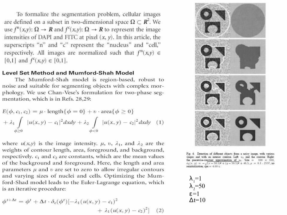
λ1=1
λ2=50
ε=1∆t=10
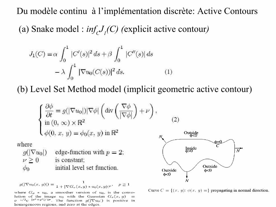
Du modèle continu à l’implémentation discrète: Active Contours
(a) Snake model : infCJ
1(C) (explicit active contour)
(b) Level Set Method model (implicit geometric active contour)

Du modèle continu à l’implémentation discrète:
The level set model with region: Infc1,c2,C
F(c1,c
2,C)
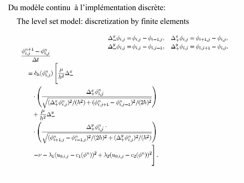
Du modèle continu à l’implémentation discrète:
The level set model: discretization by finite elements
20
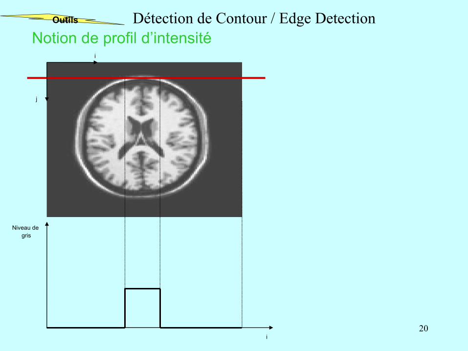
Notion de profil d’intensité
Niveau de gris
i
i
j
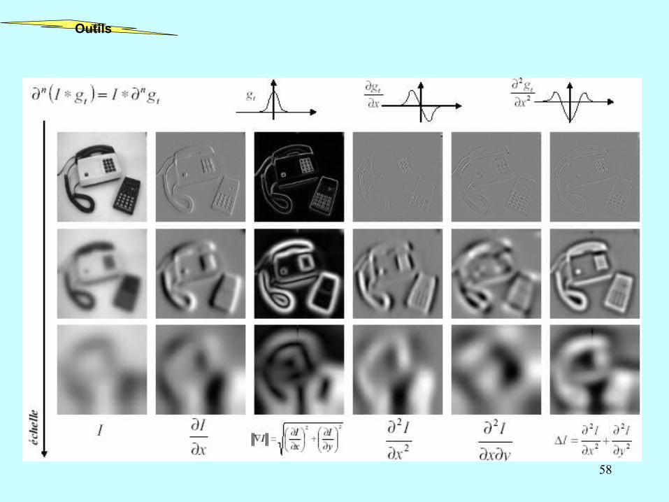
Outils Détection de Contour / Edge Detection

21
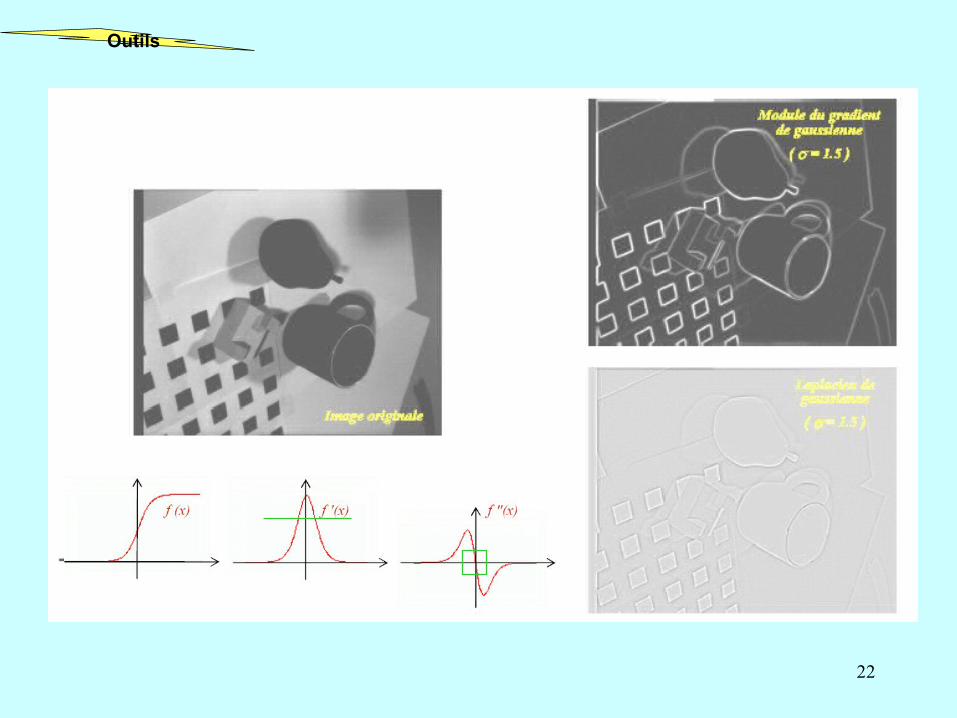
• Approche dérivative : détection des variations d'intensité locales
-> Image vue comme une fonction continue de deux variables f(x,y), échantillonée à support borné
-> Utilisation des dérivées bidimensionnelles : vecteur gradient et scalaire Laplacien
->Attention : au niveau fréquentiel, bruit ≈ contour ! en tant que discontinuité
Outils
22
Outils
23
Méthodes dérivatives de détection de contours 2D
Détection des maxima locaux de la norme du gradient dans la direction du gradient
Détection des passages par 0 du Laplacien
Outils
24
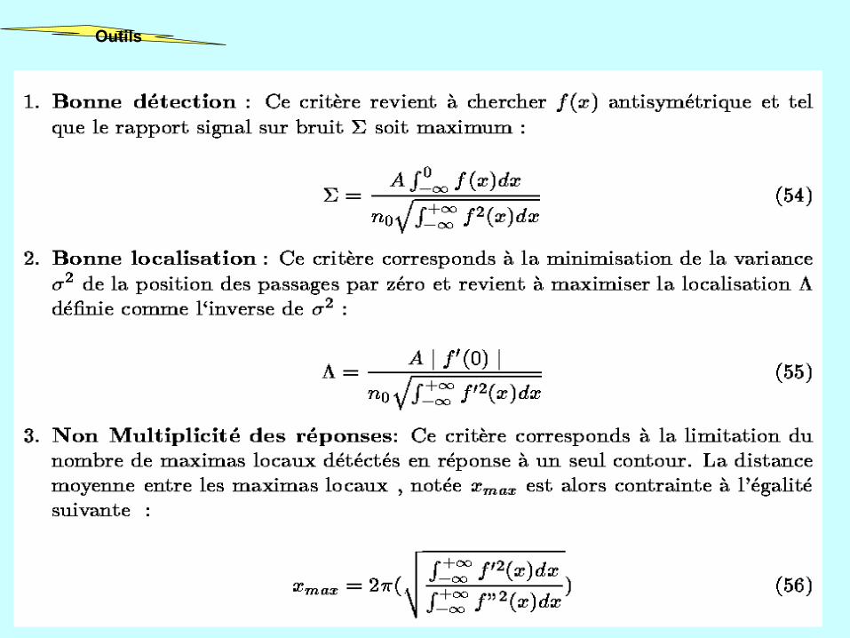
• Problèmes inverses et problèmes mal posés :Exemple : Différentiation numérique pour la détection de contoursf(x) + ε sin(ω x)Dérivation très sensible au bruit -> Régularisation [Tikhonov et Arsenin 1977]
• Un problème est bien posé si [Hadamard 1923] :1. Une solution existe2. La solution est unique3. Dépend continûment des données
• Vision = ensemble de problèmes mal posés !
Outils
25
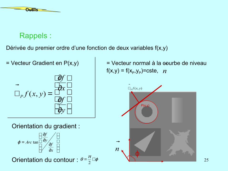
Rappels :
Dérivée du premier ordre d’une fonction de deux variables f(x,y)
= Vecteur Gradient en P(x,y)
∂∂∂∂
=∇
y
f
x
f
yxfP ),(
= Vecteur normal à la courbe de niveau f(x,y) = f(xP,yP)=cste,
Orientation du gradient :
Orientation du contour :
∂∂
∂∂
=
x
fyf
Arc tanϕ
ϕπθ +=2
n
P(x,y)
),( yxfP∇
ϕn
Outils

26
Rappels :
Dérivée du second ordre d’une fonction de deux variables f(x,y)
= Scalaire Laplacien
2
2
2
2
),(⊥∂
∂+∂∂=∆
n
f
n
fyxf
ϕϕ sincos).,(y
f
x
fnyxf
n
f
∂∂+
∂∂=∇=
∂∂
Dérivées directionnelles :
ϕϕϕϕ sincos2sincos2
2
2
2
2
2
2
yx
f
y
f
x
f
n
f
∂∂∂+
∂∂+
∂∂=
∂∂
Isotropie de l’opérateur laplacien :
2
2
2
2
2
2
2
2
),(y
f
x
f
n
f
n
fyxf
∂∂+
∂∂=
∂∂+
∂∂=∆
⊥
Outils

27
Procédure générale pour le 1er ordre
1. Obtention de deux images Im(m,n) et In(m,n)
1. Calcul de du gradient en chaque point->obtention de deux images Inorme(m,n) et Idirection(m,n)
1. Extraction des maxima locaux dans la direction du gradient->obtention de contours fins
1. Seuillage par hystérésis (seuils bas et haut)->élimination des contours parasites
),( nmIP∇
Outils

28
• Opérateurs dérivatifs du 1er ordre : Maximum du module du gradient du signal :
Filtres RIF1. Prewitt : [ 1 0 -1] 2. Sobel et Kirsh
Filtres RII1. Le filtre récursif de Canny-Deriche
• Opérateurs dérivatifs du 2ème ordre : Passage par zéro de la dérivée seconde du signal :
1. Laplacien : [1 -2 1] 2. Opérateur de Marr et Hildreth ou DoG3. Opérateur de Huertas et Medioni4. Le filtre récursif de Canny-Deriche
Outils
29
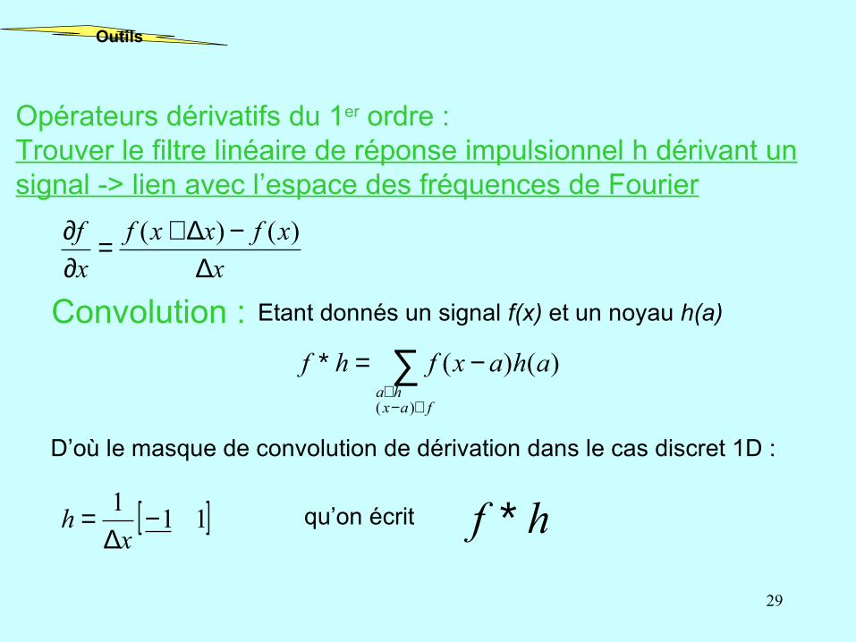
Opérateurs dérivatifs du 1er ordre : Trouver le filtre linéaire de réponse impulsionnel h dérivant un signal -> lien avec l’espace des fréquences de Fourier
x
xfxxf
x
f
∆−∆+=
∂∂ )()(
Convolution : Etant donnés un signal f(x) et un noyau h(a)
D’où le masque de convolution de dérivation dans le cas discret 1D :
∑∈−
∈
−=∗fax
ha
ahaxfhf
)(
)()(
[ ]111 −
∆=
xh qu’on écrit hf ∗
Outils
30
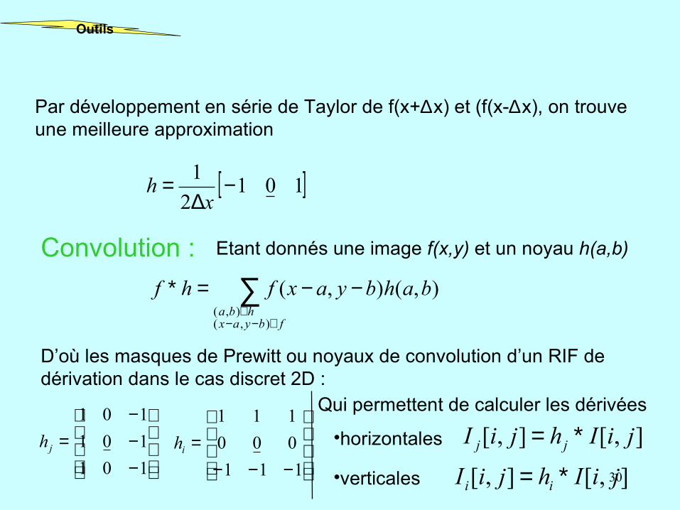
Par développement en série de Taylor de f(x+∆x) et (f(x-∆x), on trouve une meilleure approximation
[ ]1012
1 −∆
=x
h
Etant donnés une image f(x,y) et un noyau h(a,b)
∑∈−−
∈
−−=∗fbyax
hba
bahbyaxfhf
),(),(
),(),(
D’où les masques de Prewitt ou noyaux de convolution d’un RIF de dérivation dans le cas discret 2D :
−−−
=101
101
101
jh
Qui permettent de calculer les dérivées
],[],[ jiIhjiI jj ∗=
−−−=
111
000
111
ih •horizontales
],[],[ jiIhjiI ii ∗=•verticales
Convolution :
Outils
31
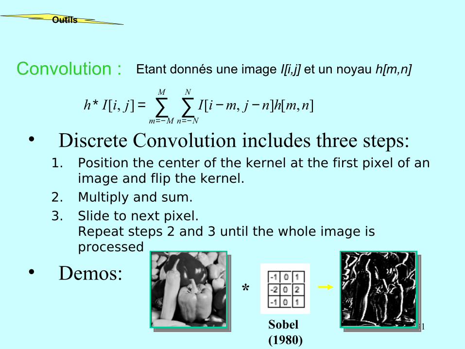
• Discrete Convolution includes three steps:1. Position the center of the kernel at the first pixel of an
image and flip the kernel. 2. Multiply and sum. 3. Slide to next pixel.
Repeat steps 2 and 3 until the whole image is processed
• Demos:*
Sobel (1980)
Etant donnés une image I[i,j] et un noyau h[m,n]
∑ ∑−= −=
−−=∗M
Mm
N
Nn
nmhnjmiIjiIh ],[],[],[
Convolution :
Outils
32
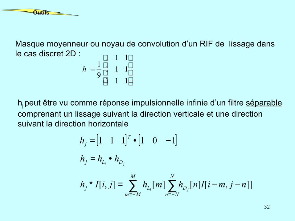
hj peut être vu comme réponse impulsionnelle infinie d’un filtre séparable comprenant un lissage suivant la direction verticale et une direction suivant la direction horizontale
[ ] [ ]101111 −•= Tjh
Masque moyenneur ou noyau de convolution d’un RIF de lissage dans le cas discret 2D :
=
111
111
111
9
1h
ji DLj hhh •=
∑ ∑−= −=
−−=∗M
Mm
N
NnDLj njmiInhmhjiIh
ji]],[][][],[
Outils

33
Quid d’un RII ?
Outils
I(x)=Au-1(x-x
0)+n(x)
34
Outils

35
Outils
36
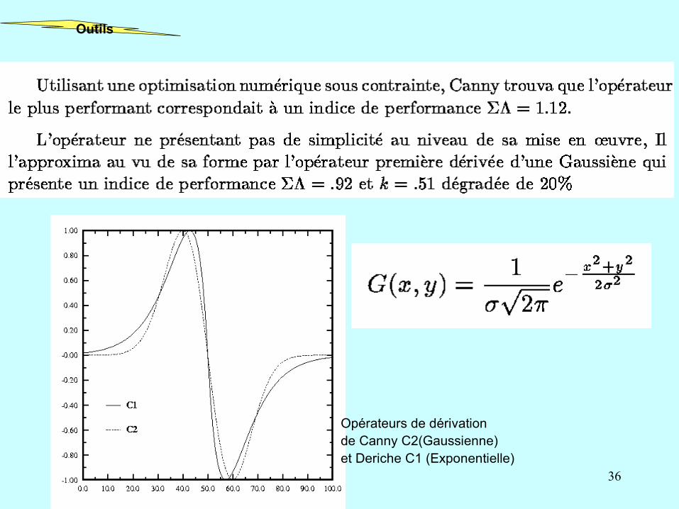
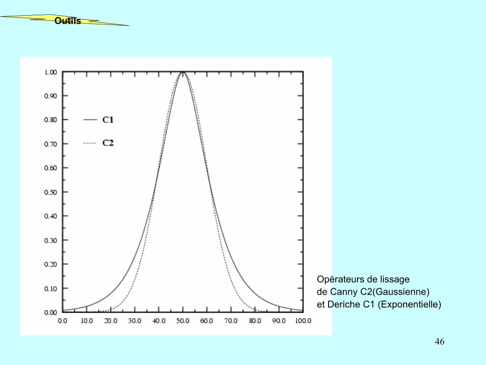
Opérateurs de dérivation de Canny C2(Gaussienne)et Deriche C1 (Exponentielle)
Outils
37
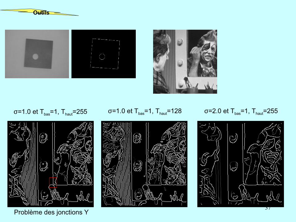
σ=1.0 et Tbas=1, Thaut=255 σ=1.0 et Tbas=1, Thaut=128 σ=2.0 et Tbas=1, Thaut=255
Problème des jonctions Y
Outils
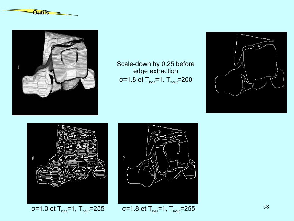
38σ=1.0 et Tbas=1, Thaut=255 σ=1.8 et Tbas=1, Thaut=255
Scale-down by 0.25 before edge extraction
σ=1.8 et Tbas=1, Thaut=200
Outils

39
3
Outils

40
3
Le cas 1 (ω ->0) est optimal, ce qui correspond au filtre de RII
xSxexf α−=)(
Comment l'implémenter sous la forme d'un RII ?
Outils
41
f+(n)
Outils
42
Ces deux transformées en Z correspondent à deux fonctions de transfert de filtres récursifs stables de second ordre.
Le premier opérant de gauche à droite F+ et le second de la droite vers la gauche F-
Outils
43
Outils

44
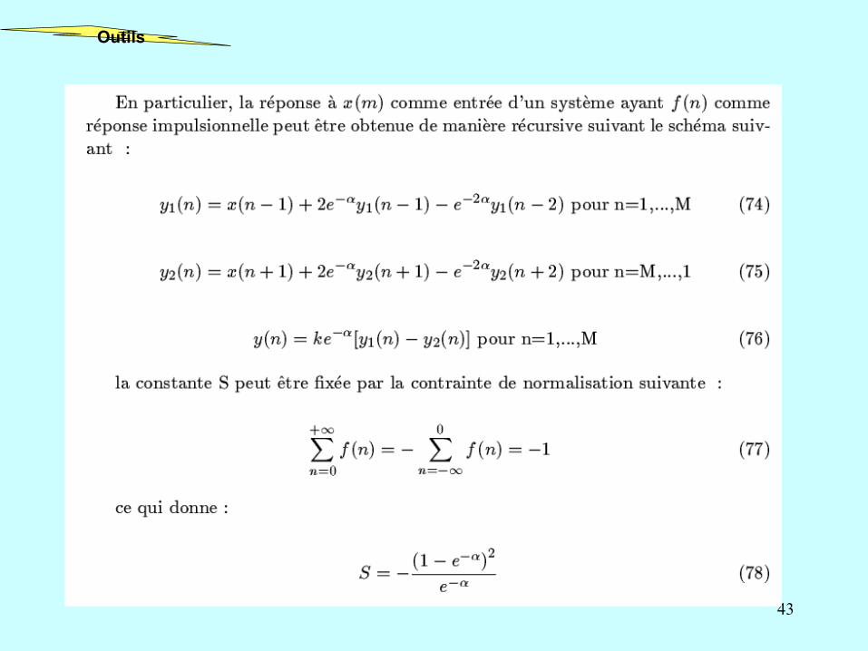
Équations récursives :
•Nombre d'opérations requis par point très faible : 5
•Nombre d'opérations requis indépendant de la résolution à laquelle les contours doivent être détectés alors que la forme du filtre (α) peut changer
Implémentation RIF pour α = 0.5 -> Masque 2N+1 de taille 57
Implémentation RIF pour α = 0.25 -> Masque 2N+1 de taille 105
•Pas d'effet de troncature du RIF
Outils

45
Noyau de lissage possible : primitive du noyau de dérivation f
( ) xexkxh
αα −+= 1)(
Outils
46
Opérateurs de lissagede Canny C2(Gaussienne)et Deriche C1 (Exponentielle)
Outils
47
Outils
48
Outils
49
Outils

50
•Lissage de l'image
•Dérivation en x de l'image
•Dérivation en y de l'image : ai <-> a i+4 et c1<->c2
Avec
Outils
51
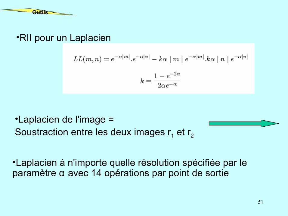
•RII pour un Laplacien
•Laplacien de l'image = Soustraction entre les deux images r1 et r2
•Laplacien à n'importe quelle résolution spécifiée par le paramètre α avec 14 opérations par point de sortie
Outils

52
Outils
53
Outils

54
Outils

55
Outils
56
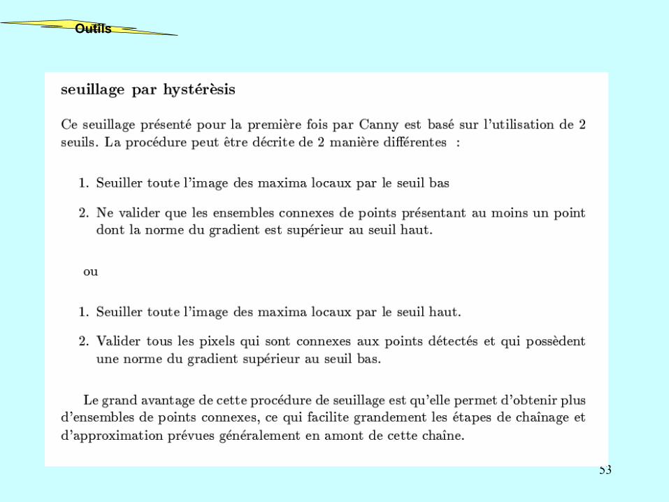
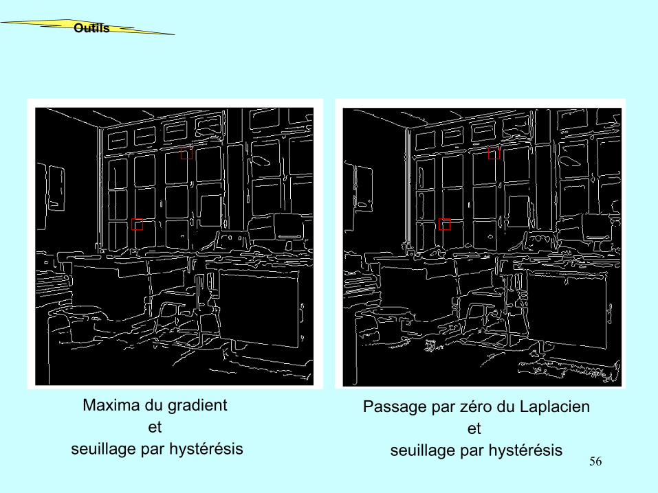
Maxima du gradient et
seuillage par hystérésis
Passage par zéro du Laplacienet
seuillage par hystérésis
Outils
57
Outils
58
Outils

59
Outils
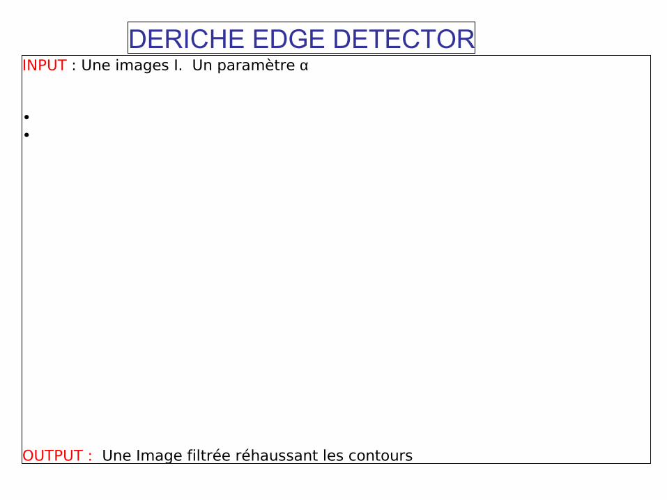
DERICHE EDGE DETECTOR
INPUT : Une images I. Un paramètre α
• •
OUTPUT : Une Image filtrée réhaussant les contours

• 75 Parkinson patients + 75 controls– EP2D2 DTI1 4mm - 351 images/patient– T2SE3 DTI overlay high resolution - 27
images/patient– AX FLAIR4 pat2 - 19 images/patient– T1 MPR5 axial 4mm - 44 images/ patient
1 DTI – Diffusion Tensor Image2 EP2D – Echo Planar 2D DTI3 T2SE – Tensor 2 Scale Echography4 AxFLAIR- Axial direction for Flair (white matter lesions)5 T1MPR – Tensor 1 Multi Planar Reconsturction
Early Detection of Parkinson Disease

Original preprocessed EP2D image
Grey matter image
SPM segmented registred image
White matter image
Atlas registred image
Early Detection of Parkinson Disease
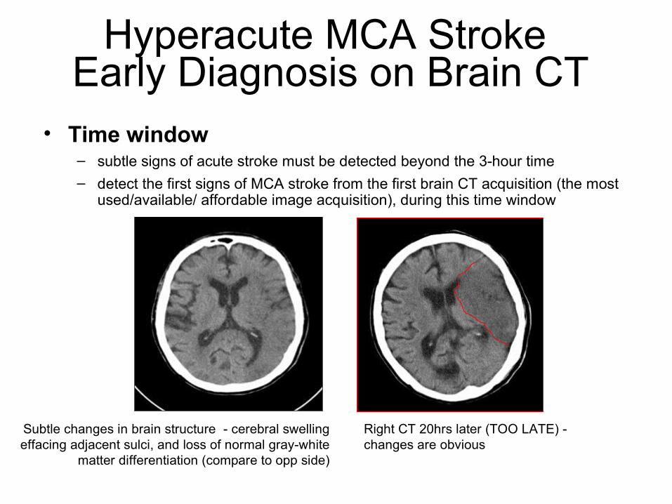
Hyperacute MCA Stroke Early Diagnosis on Brain CT
• Time window – subtle signs of acute stroke must be detected beyond the 3-hour time
– detect the first signs of MCA stroke from the first brain CT acquisition (the most used/available/ affordable image acquisition), during this time window
Subtle changes in brain structure - cerebral swelling effacing adjacent sulci, and loss of normal gray-white
matter differentiation (compare to opp side)
Right CT 20hrs later (TOO LATE) - changes are obvious
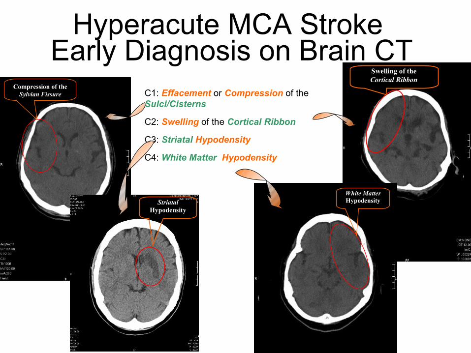
Compression of the Sylvian Fissure
Swelling of the Cortical Ribbon
Striatal Hypodensity
White Matter Hypodensity
C1: Effacement or Compression of the Sulci/Cisterns
C2: Swelling of the Cortical Ribbon
C3: Striatal Hypodensity
C4: White Matter Hypodensity
Hyperacute MCA Stroke Early Diagnosis on Brain CT
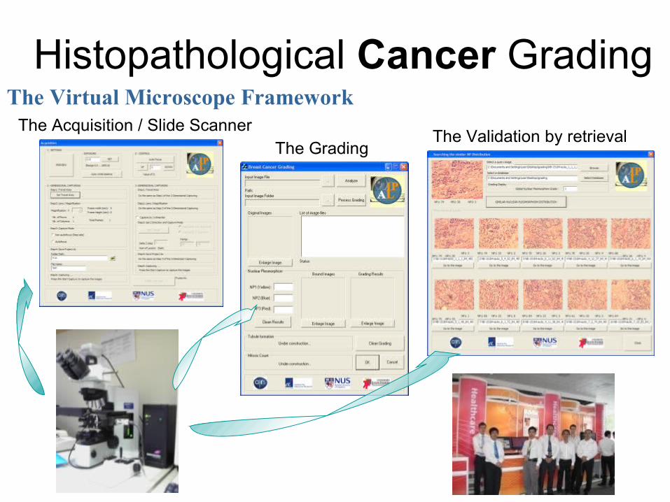
Histopathological Cancer Grading
The Acquisition / Slide ScannerThe Grading
The Validation by retrieval
The Virtual Microscope Framework

Tubule formation score
Mitosis count
Nuclear pleomorphism score
Frame grading
Individual frame
Semantic indexing
Pathologist
Semantic query Similarity
“ Show me the frames with the most mitotic
cells”
Medical rules
+ Context
Histopathological Cancer Grading
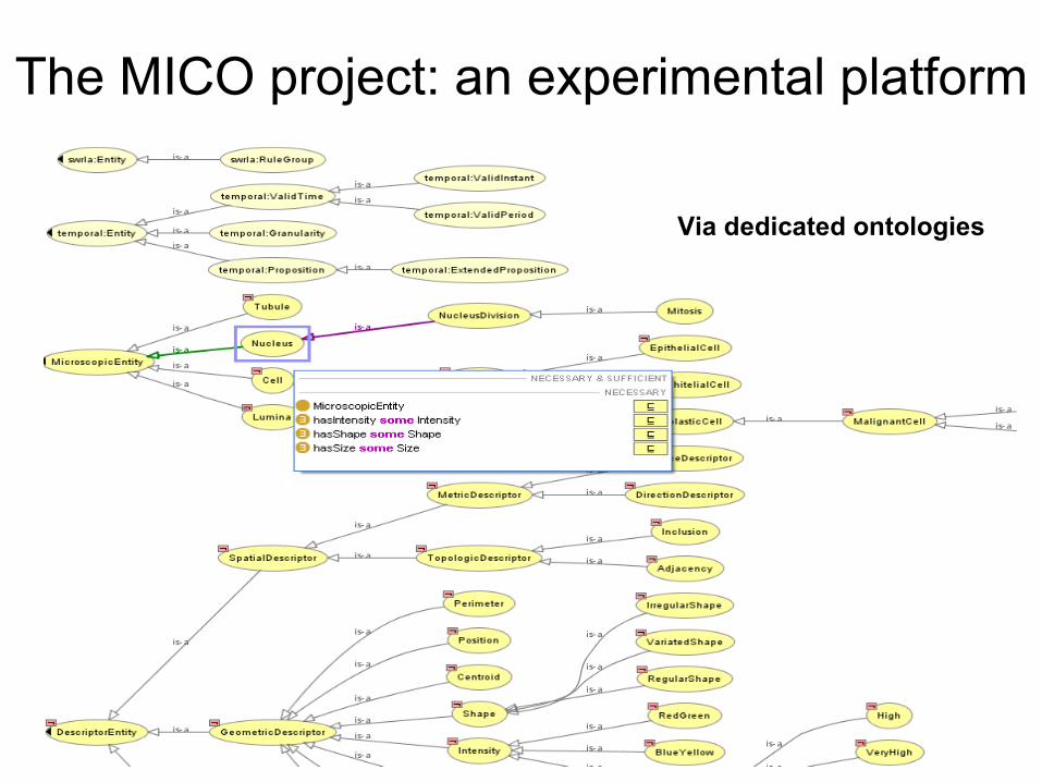
The MICO project: an experimental platform
Via dedicated ontologies

The MICO project: an experimental platform
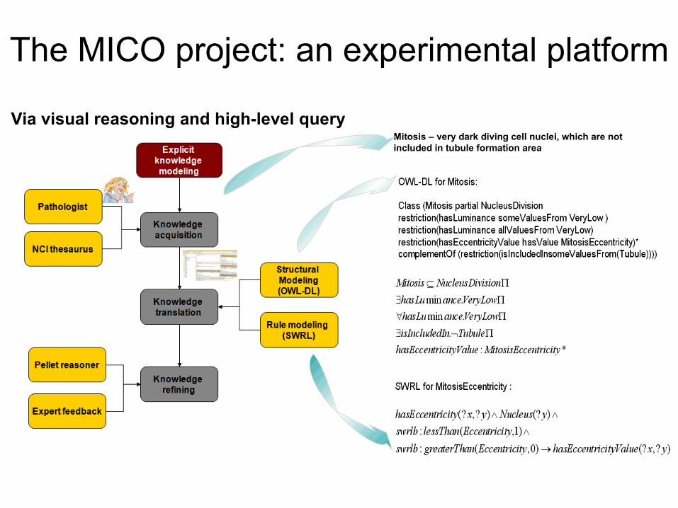
Mitosis – very dark diving cell nuclei, which are not included in tubule formation area
The MICO project: an experimental platform
Via visual reasoning and high-level query
The MICO project: an experimental platform

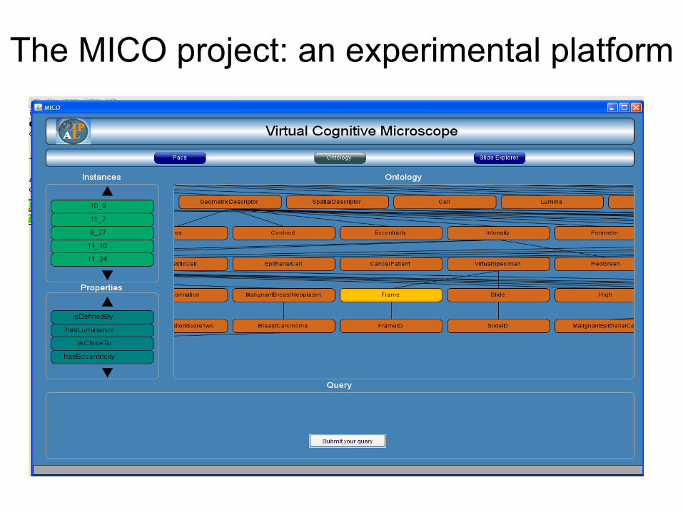
The MICO project: an experimental platform

Ouvrages de références :
“Analyse d'images : Filtrage et Segmentation”, Cocquerez and al., Ed. Dunod, 1995 (ouvrage de base : exposé des différentes techniques de traitement d'images appliquées à la segmentation)
“Le traitement des images”, H. Maître, Hermes Science Publications , 2003(ouvrage de référence écrit par un maître national du sujet : beaucoup d’explications approfondies du phénomène image à tous les niveaux et notamment traitement du signal)
“Computer Vision : a modern approach”, Forsyth and Ponce, International Edition,Prentice Hall, 2003
« Advances in Bio-imaging: From Physics to Signal Processing Understanding Issues: state of the art and challenges », Springer, 2011, 242 pages, N. Loménie et al. Editors.
Bibliographie
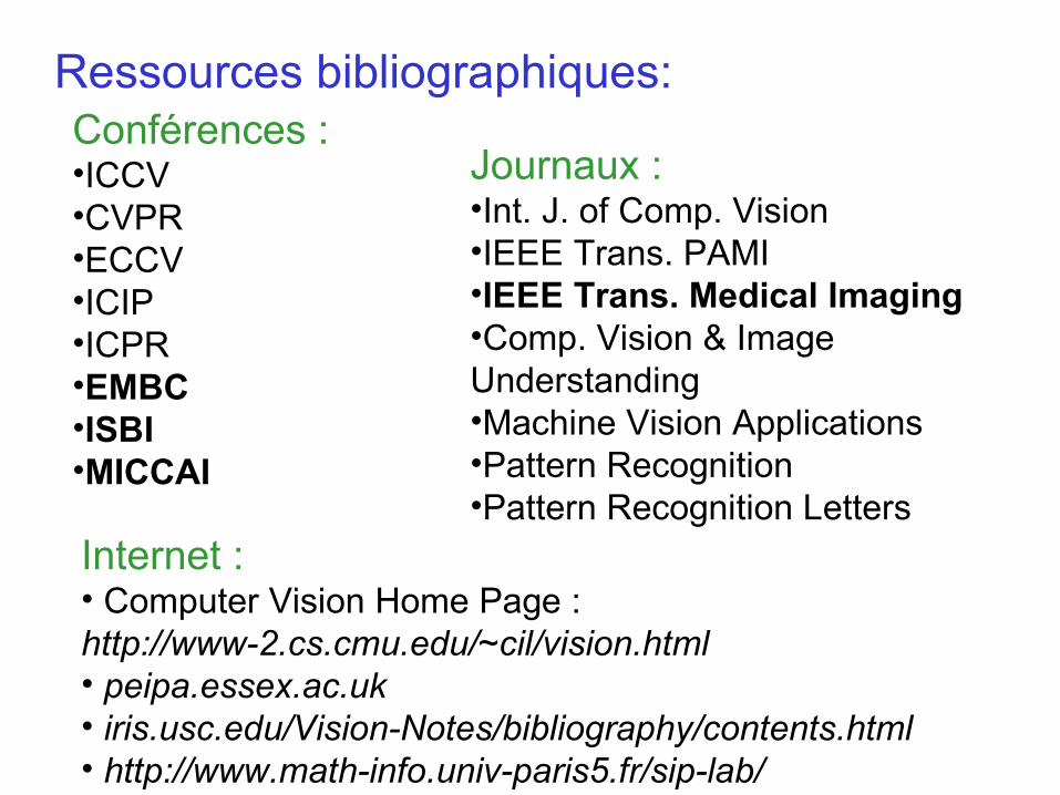
Conférences :•ICCV•CVPR•ECCV•ICIP•ICPR•EMBC•ISBI•MICCAI
Ressources bibliographiques:
Journaux :•Int. J. of Comp. Vision•IEEE Trans. PAMI•IEEE Trans. Medical Imaging•Comp. Vision & Image Understanding•Machine Vision Applications•Pattern Recognition•Pattern Recognition Letters
Internet :• Computer Vision Home Page : http://www-2.cs.cmu.edu/~cil/vision.html• peipa.essex.ac.uk• iris.usc.edu/Vision-Notes/bibliography/contents.html• http://www.math-info.univ-paris5.fr/sip-lab/
Top Related