


Languages
Pages
Legal


Simulations of Polarimetric Radar Signatures of a Supercell StormUsing a Two-Moment Bulk Microphysics Scheme
YOUNGSUN JUNG AND MING XUE
School of Meteorology, and Center for Analysis and Prediction of Storms, University of Oklahoma,
Norman, Oklahoma
GUIFU ZHANG
School of Meteorology, University of Oklahoma, Norman, Oklahoma
(Manuscript received 6 January 2009, in final form 6 July 2009)
ABSTRACT
A new general polarimetric radar simulator for nonhydrostatic numerical weather prediction (NWP)
models has been developed based on rigorous scattering calculations using the T-matrix method for reflec-
tivity, differential reflectivity, specific differential phase, and copolar cross-correlation coefficient. A con-
tinuous melting process accounts for the entire spectrum of varying density and dielectric constants. This
simulator is able to simulate polarimetric radar measurements at weather radar frequency bands and can take
as input the prognostic variables of high-resolution NWP model simulations using one-, two-, and three-
moment microphysics schemes. The simulator was applied at 10.7-cm wavelength to a model-simulated
supercell storm using a double-moment (two moment) bulk microphysics scheme to examine its ability to
simulate polarimetric signatures reported in observational studies. The simulated fields exhibited realistic
polarimetric signatures that include ZDR and KDP columns, ZDR arc, midlevel ZDR and rhy rings, hail sig-
nature, and KDP foot in terms of their general location, shape, and strength. The authors compared the
simulation with one employing a single-moment (SM) microphysics scheme and found that certain signatures,
such as ZDR arc, midlevel ZDR, and rhy rings, cannot be reproduced with the latter. It is believed to be
primarily caused by the limitation of the SM scheme in simulating the shift of the particle size distribution
toward larger/smaller diameters, independent of mixing ratio. These results suggest that two- or higher-moment
microphysics schemes should be used to adequately describe certain important microphysical processes. They
also demonstrate the utility of a well-designed radar simulator for validating numerical models. In addition, the
simulator can also serve as a training tool for forecasters to recognize polarimetric signatures that can be re-
produced by advanced NWP models.
1. Introduction
Supercell thunderstorms have received significant at-
tention from the meteorology community because they
often cause serious damage from the associated torna-
does, large hail, strong winds, and/or heavy precipi-
tation. Many observational studies have focused mainly
on understanding the time evolution of storm structure,
microphysical characteristics, and dynamics using radar
reflectivity and radial velocity data (e.g., Browning and
Donaldson 1963; Browning 1964; Lemon and Doswell
1979; Marwitz 1972; Musil et al. 1986; Ray et al. 1981;
Brandes 1978, 1984, 1993). Numerical studies have tried
to simulate such supercell storms and aid in the under-
standing of storm evolution and dynamics (e.g., Klemp
and Wilhelmson 1978; Klemp et al. 1981; Weisman and
Klemp 1982; Rotunno 1981; Klemp and Weisman 1983).
Recently, research has demonstrated that the storm mi-
crophysical processes and properties can be better un-
derstood with polarimetric radar data (e.g., Bringi et al.
1986; Hubbert et al. 1998; Romine et al. 2008; Kumjian
and Ryzhkov 2008, 2009, hereinafter KR08 and KR09,
respectively).
Although conventional and polarimetric radar obser-
vations offer important insights into storms, observa-
tions are often insufficient to provide details on the
storms because of various limitations. Such limitations
Corresponding author address: Youngsun Jung, Center for
Analysis and Prediction of Storms, National Weather Center, Suite
2500, 120 David L. Boren Blvd., Norman, OK 73072.
E-mail: [email protected]
146 J O U R N A L O F A P P L I E D M E T E O R O L O G Y A N D C L I M A T O L O G Y VOLUME 49
DOI: 10.1175/2009JAMC2178.1
� 2010 American Meteorological Society
include the lack of complete spatial coverage because of
beam blockage, radar cone of silence, or lack of signal
returns in weak echo regions, sampling noise and signal
attenuation, or insufficient spatial and temporal resolu-
tions. In addition to these external factors, reflectivity and
polarimetric measurements provide only high-moment
bulk properties of all hydrometeors in the radar resolu-
tion volume, and Doppler radial velocity offers only the
wind component projected in the direction of the radar
beams.
On the other hand, numerical models allow meteo-
rologists to study details that are not directly observed
by current observational platforms with high temporal
and spatial resolutions. They can help substantiate find-
ings from observational studies. Numerical models also
can be used to help develop new theories. Most of all, the
numerical model is of primary importance in modern
weather forecasting. However, the numerical solutions
must be validated with appropriate observations; a com-
plementary relationship exists between observations and
numerical models.
For direct comparisons between model output and
radar observations, the model variables are often con-
verted into the form of observations using a radar simu-
lator (Jung et al. 2008a, hereinafter JZX08; Pfeifer et al.
2008), which also acts as the forward observation op-
erator in data assimilation systems. The radar simulator
should be accurate, consistent with model microphys-
ics, and make use of all relevant information available
in the model.
Most existing polarimetric radar simulators deal only
with rain or dry ice exclusively (e.g., Brandes et al. 2004;
Ryzhkov et al. 1998; Vivekanandan et al. 1994; Zhang
et al. 2001; Capsoni et al. 2001); the literature covers only
a handful of complete polarimetric radar simulators that
utilize a full set of parameters available in the numerical
model. Huang et al. (2005), in a short conference paper,
reported on a simulator based on T-matrix scattering
calculations (Waterman 1969; Vivekanandan et al. 1991).
It used output from the Regional Atmospheric Modeling
System (RAMS) employing a two-moment microphysics
scheme (Walko et al. 1995; Meyers et al. 1997). In that
paper, the authors employed a simple melting treatment
for ice species with fixed fractions of water and ice (and
air for graupel) based on the height or air temperature.
Recently, JZX08 developed a polarimetric radar sim-
ulator utilizing the fitting of the scattering amplitudes of
rain calculated using T-matrix codes in a power-law form
of the particle size, while Rayleigh scattering approxi-
mation is used for ice for a single-moment microphysics
scheme. In the work, the authors introduced a new
melting ice model with a continuously varying density of
ice particles and the fractional water in the ice. In this
melting ice model, wet ice particles, such as rain–snow or
rain–hail mixtures, are constructed when rainwater co-
exists with snow or hail. In the model, the fractional
water in the ice is determined by the relative amount
between rainwater and snow or hail. For the data as-
similation purpose reported in that paper, the researchers
had to use curves fitted to precalculated data or Rayleigh
scattering assumption in the simulator for efficiency;
therefore, it is not a general purpose simulator.
Pfeifer et al. (2008) also proposed a polarimetric sim-
ulator called Synthetic Polarimetric Radar (SynPolRad)
based on the T-matrix method. SynPolRad is coupled
with a single-moment microphysics scheme with various
assumptions about the hydrometeor drop size distribu-
tions (DSDs). The authors determined a fixed value for
water fraction in wet ice hydrometeors by fitting the
values of simulated polarimetric variables to their ex-
pected values within a certain range of observations.
However, the dielectric model used by them is physically
questionable because the dielectric constant was calcu-
lated ‘‘as water inside an ice matrix inside air matrix,’’
which cannot correctly represent the significant contri-
bution from the meltwater shell. Additionally, the specific
differential phase, which is a very useful polarimetric
measurement, is not included in SynPolRad.
Although these simulators have their own strengths
and weaknesses, they show that polarimetric radar sim-
ulators can be useful for evaluating model microphysics.
Furthermore, a computationally optimized simulator can
serve as the forward observation operator in data as-
similation systems.
In this study, we develop a radar simulator that is
more general than that described in JZX08; it employs
the full T-matrix scattering method for both rain and
ice hydrometeors and allows for the specification of any
radar wavelength for scattering calculations. In this
study, the wavelength is set to 10.7 cm, that of the U.S.
operational Weather Surveillance Radar-1988 Doppler
(WSR-88D) radars. Model prognostic variables associ-
ated with single-, double-, or three-moment (SM, DM,
and TM, respectively) bulk microphysics schemes (simply
‘‘scheme’’ hereinafter) can be used as inputs. The polar-
imetric variables simulated include reflectivity at the
horizontal and vertical polarizations (ZH and ZV), dif-
ferential reflectivity ZDR, specific differential phase KDP,
and the copolar cross-correlation coefficient at zero-lag
rhy(0).
A recent study of Milbrandt and Yau (2006), Dawson
et al. (2007, 2010), and Dawson (2009) found that su-
percell thunderstorms with a more realistic reflectivity
structure and cold pool strength can be obtained with
a multimoment (MM) microphysics scheme, with most
improvement achieved when moving from SM to DM
JANUARY 2010 J U N G E T A L . 147

scheme. Their results show that the DM and TM simu-
lations are qualitatively similar in terms of cold pool
structure, reflectivity pattern in the forward flank regions,
the amount of total cooling in the low-level downdraft,
the characteristics of drop size distribution parameters,
and the origin of the air in the surface cold pool. On the
other hand, the SM runs show large variability within
these runs, depending on the choice of the intercept pa-
rameter values. Briefly, the MM schemes produce weaker
and moister cold pools and more extended forward flank
regions. Their trajectory analyses show that the air near
the surface cold pool originates from above the bound-
ary layer (2–3 km AGL) in the SM runs while it comes
from about 1 km AGL in the MM runs. The mean-mass
diameter of raindrops in the low-level downdraft is sig-
nificantly larger in the MM runs than in the SM runs.
These results show that the storm microphysics evolve in
very different ways in the SM and MM schemes. The
polarimetric measurement may provide an additional
means to evaluate the performance of different micro-
physics schemes.
In this study, we apply our newly developed simulator
to a supercell storm simulated using DM and SM schemes
and examine their ability to reproduce characteristic
polarimetric signatures commonly found in polarimetric
radar observations. The TM simulation is not investi-
gated here, based on the similarity between the DM and
TM simulations of Dawson (2009) and Dawson et al.
(2010), but can be explored in future studies. Radial ve-
locity is included in our emulator but not discussed in this
paper, as we focus only on the polarimetric signatures.
This paper is organized as follows: in section 2, we
discuss the polarimetric radar simulator and assump-
tions about the DSDs. In section 3, the numerical sim-
ulation of the supercell storm is described. In section 4,
we present the polarimetric radar simulations and the
associated polarimetric signatures and compare them
with the results using an SM scheme. The results are
summarized in section 5.
2. Polarimetric radar data simulator
The simulator developed in this study is more com-
plex and general than the one reported in JZX08. As
discussed in JZX08, the DSD-related parameters within
the simulator should be consistent with those used in the
numerical model. Within the multimoment microphys-
ics scheme of Milbrandt and Yau (2005a,b) used in this
study and Dawson (2009), the DSDs of each species,
n(D), are modeled by a gamma distribution that con-
tains three free parameters,
n(D) 5 N0Dae�LD, (1)
where D is the particle or drop diameter, and N0, a, and
L are the intercept, shape, and slope parameters, re-
spectively. In brief, many SM schemes used in opera-
tional systems assume a Marshall and Palmer (1948)
distribution with a 5 0 and a fixed N0, which is an in-
verse exponential distribution. The predicted variable,
hydrometeor mixing ratio q, monotonically determines
L and thus n(D). On the other hand, the DM scheme
used in this study predicts q and the total number of
particles Nt, which allows for the independent change of
N0 and L while a is fixed. Researchers reported that N0
can vary significantly among precipitation systems and
even within the same system (e.g., Waldvogel 1974;
Gilmore et al. 2004). Therefore, the DM scheme may be
more appropriate for the simulation of precipitation
systems. The TM scheme usually predicts q, Nt, and the
radar reflectivity factor Z. All three DSD parameters—
N0, L, and a—vary freely in time and space, and the
width of the DSD can practically vary over a wide range
with the TM scheme. For more detailed information on
the various microphysical parameterizations, the reader
is referred to Milbrandt and Yau (2005a) and Dawson
et al. (2010).
In the simulator, fixed densities of 1000, 100, and
913 kg m23 are assumed for rain (rr), snow (rs), and hail
(rh), respectively, as in the prediction model. Additional
particle characteristics are needed to simulate polari-
metric variables, such as the shape, the statistical prop-
erties of the particle orientation, and the ice–water
composition of the hydrometeors. Since these parame-
ters are not explicitly specified in the prediction model,
assumptions have to be made, based on as much avail-
able information as possible. The assumptions we make
here are largely inherited from JZX08. Briefly, rain-
drops, snow aggregates, and hailstones are all assumed
as oblate spheroids falling with the major axis aligned
horizontally. The oblateness depends on the size of a
raindrop while a fixed axis ratio of 0.75 is assumed for
snow aggregate and hailstone. [Other axis ratios for
hailstones, such as the one based on the Oklahoma hail-
storms studied by Knight (1986), are also available as
options in the radar simulator.] The mean canting angles
of all hydrometeor types are assumed to be 08. The
standard deviation (SD) of the canting angle is assumed
to be 08 for raindrops, 208 for snow aggregates, and a
function of the water content in melting hail with maxi-
mum 608 for dry hailstones. For more detailed informa-
tion, the reader is referred to JZX08.
To benefit from the T-matrix scattering calculations,
which do not allow for analytical integration, we carry
out a numerical integration of the scattering amplitudes
over the DSD for all hydrometeor types in the simulator.
This allows us to deploy the revised axis ratio relation
148 J O U R N A L O F A P P L I E D M E T E O R O L O G Y A N D C L I M A T O L O G Y VOLUME 49

based on the observations for rain (Brandes et al. 2002),
which yields more spherical shapes consistently at all sizes
when compared with that given in Zhang et al. (2001),
r 5 0.9951 1 0.025 10D� 0.036 44D2
1 0.005 303D3 � 0.000 249 2D4. (2)
While a few other relationships, including the ones given
by Green (1975) and Beard et al. (1991), are available in
the simulator as alternative user-selectable options, new
relationships can easily be added as well.
Within the scattering calculations, the maximum sizes
of rain drops (Dmax,r), snow aggregates (Dmax,s), and
hailstones (Dmax,h) are assumed to be 8, 30, and 70 mm,
respectively. These size ranges are partitioned into
100 bins. For rain, dry snow, and dry hail, the forward
and backward scattering amplitudes along the major and
minor axes with assumed drop shape are calculated at
the center of each size bin and stored in lookup tables.
For melting species, lookup tables are constructed at
uniform water fraction intervals, which is 5% in this
study. The same melting ice and dielectric constant
models developed in JZX08 are employed in the scat-
tering calculation. For example, for a melting snow ag-
gregate with a specified water fraction, the density and
dielectric constant of that particle are calculated and
used to compute the forward and backward scattering
amplitudes at each size bin with that water fraction.
These scattering amplitudes are then integrated over
the DSD when the model mixing ratios (and the total
number concentration for DM and the additional sixth
moment of DSD for TM schemes) are given as input.
We employ formulations for radar reflectivity factors
at horizontal and vertical polarizations that are more
exact than those in JZX08 by including the complex
scattering amplitude in the calculations as follows (Zhang
et al. 2001):
Zh,x
54l4
p4jKwj2ðDmax,x
0
fAj fa,x
(p)j2 1 Bj fb,x
(p)j2 1 2C Re[fa,x
(p) f *b,x
(p)]gn(D) dD (mm6 m�3) (3)
and
Zy,x
54l4
p4 Kw
�� ��2ðDmax,x
0
fBjfa,x
(p)j2 1 Aj fb,x
(p)j2 1 2C Re[fa,x
(p) f *b,x
(p)]gn(D) dD (mm6 m�3), (4)
where
A 5 hcos4fi5 1
8(3 1 4 cos2fe�2s2
1 cos4fe�8s2
),
B 5 hsin4fi5 1
8(3� 4 cos2fe�2s2
1 cos4fe�8s2
),
and
C 5 hsin2f cos2fi5 1
8(1� cos4fe�8s2
),
and subscript x can be r (for rain) or rs (for rain–snow
mixture), ds (for dry snow), rh (for rain–hail mixture),
or dh (for dry hail). Here, fa(p) and fb(p) are complex
backscattering amplitudes for polarizations along the
major and minor axes, respectively, and fa* and fb* are
their respective conjugates. Here, Re[� � �] represents the
real part of the complex number, and j� � �j means the
magnitude of the value between single bars; h� � �imeans
that an ensemble average is taken over canting angles,
and n(D) defines the DSD and is the number of particles
per unit volume of air and unit bin size. Truncation is
applied at maximum sizes of raindrop, snow aggregates,
and hailstone when integration over DSD is performed.
The mean canting angle is f, the standard deviation of
the canting angle is s, the radar wavelength is l, and the
dielectric factor for water is Kw 5 0.93.
The same equations for logarithmic reflectivity at hor-
izontal and vertical polarizations and differential reflec-
tivity of JZX08 are used here [see their Eqs. (14)–(16),
respectively]. The value ZDR is a good indicator of the
mean shape of hydrometeors and depends on their rel-
ative orientation to the radar beam. Therefore, DSD
changes toward larger or smaller drop sizes can be
roughly inferred from the ZDR value.
The specific differential phase is defined as
KDP,x
5180l
p
ðDmax,x
0
Ck
Re[fa,x
(0)� fb,x
(0)]n(D) dD (8 km�1), (5)
JANUARY 2010 J U N G E T A L . 149
where Ck
5 hcos2fi 5 cos2fe�2s2. Note that fa(0) and
fb(0) here are forward scattering amplitudes for polari-
zations along the major and minor axes, respectively.
The KDP is regarded as more useful in quantitative pre-
cipitation estimation because it is more linearly pro-
portional to the rainfall rate than reflectivity. However,
the KDP field is often very noisy in weak rain regions and
is vulnerable to errors.
The cross-correlation coefficient (Ryzhkov 2001; Jung
2008, hereinafter J08) is defined as
rhy
5jZ
hy,r1 Z
hy,ds1 Z
hy,dh1 Z
hy,rs1 Z
hy,rhj
[(Zh,r
1 Zh,ds
1 Zh,dh
1 Zh,rs
1 Zh,rh
)(Zy,r
1 Zy,ds
1 Zy,dh
1 Zy,rs
1 Zy,rh
)]1/2, (6)
where the numerator is given as a product of two orthogonal copolar components of the radar signals and
computed as
Zhy,x
54l4
p4jKwj2ðDmax,x
0
fC[j fa,x
(p)j2 1 j fb,x
(p)j2] 1 A[fa,x
(p) f *b,x
(p)] 1 B[ fb,x
(p) f *a,x
(p)]gn(D) dD (mm6 m�3).
(7)
Cross-correlation coefficient rhy is very useful in detect-
ing the melting layer since it is sensitive to the presence of
randomly oriented wet ice particles; rhy is very high for
pure rain and relatively high for low-density dry ice par-
ticles, but is much lower in the presence of large, wet
hailstones. The simpler versions of Eqs. (3), (4), and (7)
can be found in J08, where the empirical coefficient
r0,x, which is less than unity, is introduced in the second
and third terms within the integral of Eq. (7) to better
fit the observed rhy range, and Rayleigh assumptions
are employed for snow aggregate and hailstones for
efficiency.
When creating observations on the radar elevation
planes, the effective earth radius model (Doviak and
Zrnic 1993) is used to take into account beam bending,
and a Gaussian beam weighting function described in
Xue et al. (2006) is used in the vertical direction. The
error model described in Xue et al. (2007) and Jung et al.
(2008b, hereinafter JXZS08) is optional for adding
simulated observation errors. In this study, error-free
polarimetric variables are created at each grid point.
3. Numerical simulation
Similar to the truth simulation used in JXZS08, an
idealized supercell storm is initialized by a thermal
bubble placed in a horizontally homogeneous environ-
ment defined by the sounding of the 20 May 1977 Del
City, Oklahoma, supercell storm (Ray et al. 1981). The
storm is simulated using the Advanced Regional Pre-
diction System (ARPS; Xue et al. 2000, 2001, 2003),
which is a fully compressible and nonhydrostatic atmo-
spheric prediction model. The MM schemes described in
Milbrandt and Yau (2005a,b) have been implemented
recently in ARPS (Dawson et al. 2007; Dawson 2009)
and are used in this study. This Milbrandt–Yau scheme
is referred to as MY05 hereinafter.
With the DM option of the MY05, the ARPS predicts
three velocity components u, y, and w; potential tem-
perature u; pressure p; mixing ratio of water vapor qy;
mixing ratios of cloud water, rainwater, cloud ice, snow
aggregate, and hail (qc, qr, qi, qs, and qh, respectively);
and their total number concentrations (Ntc, Ntr, Nti, Nts,
and Nth, respectively). The graupel category originally
included in the MY05 package is turned off to maintain
consistency with our previous experiments (JXZS08 and
JZX08). The turbulent kinetic energy is also predicted
by the model and is used in the 1.5-order subgrid-scale
turbulence closure scheme.
The initiating bubble has an ellipsoidal shape and has
4-K maximum temperature perturbation, is 10 km long
and 1.5 km high in radius, and is centered at x 5 48 km,
y 5 48 km, and z 5 1.5 km in a 158 3 128 3 16 km3
model domain. Radiation, rigid wall with a wave-
absorbing layer, and free-slip condition are applied to
the lateral, top, and bottom boundaries, respectively.
A few changes are made to the configurations used
in JXZS08 and JZX08 to accommodate the use of the
DM scheme. Following Dawson et al. (2010), the smaller
horizontal grid spacing of 1.0 km is used with the vertical
grid spacing of 0.5 km. Constant winds of u 5 1 m s21
and y 5 13 m s21 are subtracted from the original
sounding to keep the storm near the center of the domain.
A fourth-order monotonic computational mixing (Xue
2000) is used to prevent the Gibbs phenomenon.
The MM scheme of MY05 assumes that each hydro-
meteor type has a constant density. The default values
for rain, snow, and hail are 1000, 100, and 913 kg m23 but
150 J O U R N A L O F A P P L I E D M E T E O R O L O G Y A N D C L I M A T O L O G Y VOLUME 49
can be altered by the user. The DSDs for all hydrometeor
types are modeled by exponential distribution in the
current study, by assuming the shape parameters for each
species to be 0; doing so maintains a consistency with the
DSDs used in the SM runs.
4. Simulated polarimetric signatures
a. Storm evolution and simulated reflectivity
Figure 1 shows the time evolution of the reflectivity
and other fields of the simulated supercell storm using
SM and DM microphysics schemes of MY05, at 250-m
altitude, where the first scalar model level above ground
is found. Briefly, the updraft quickly intensifies during
the first 20 min, with a reflectivity core greater than
40 dBZ appearing after 10 min of simulation (not shown).
While the forward flank regions continue to expand in
the next 30 min, the storm splits into two cells at around
1 h (Fig. 1b). The left-moving cell (relative to the envi-
ronmental shear vector) then continues to develop while
propagating to the northwest of the right-moving cell.
The right-moving cell is at its mature stage by 80 min of
model time and maintains its intensity for the next few
hours. In this study, we focus on the right-moving storm,
which is usually the dominant one.
As discussed in Dawson et al. (2007, 2010) and Dawson
(2009), though for a different case, the simulated re-
flectivity using the DM scheme (Figs. 1b,d,f) shows a
more realistic structure and intensity in the hook echo
and forward flank regions compared to the results of the
SM scheme (Figs. 1a,c,e). Our simulated storm using the
MY05 SM scheme is very similar to that using the Lin
et al. (1983) ice microphysics scheme shown in Fig. 2 of
Tong and Xue (2005), which used the same Del City
sounding. Compared to the simulated reflectivity ob-
tained with the DM scheme, that using the SM scheme
has a kidney shape with a narrow forward flank, while
DM produces a swirl-shaped weak echo region (WER)
wrapping around the hook echo and extends the forward
flank to the far east of the storm (Figs. 1b,d,f). Another
significant difference between the storms using the SM
and DM schemes is in the cold pool strength. SM
schemes with default DSD parameter settings tend to
produce stronger cold pools than DM schemes. Dawson
et al. (2010) showed that one of the main causes of the
strong cold pool with SM schemes is the stronger evap-
orative cooling of raindrops in the downdraft related to
the fixed, large, N0r, which corresponds to a larger num-
ber of small drops that can evaporate quickly.
A detailed evaluation of microphysics schemes is be-
yond the scope of this study. Our focus will be on the
ability of our simulator in reproducing characteristic
polarimetric signatures when using different microphys-
ics schemes.
b. Simulated polarimetric radar variables
Several unique polarimetric signatures have been
reported in observational studies of supercell storms.
They include strong ZDR and KDP columns, a midlevel
ZDR ring, a hail signature (ZDR hole), ZDR arc (ZDR
shield), midlevel rhy ring, and KDP foot (e.g., Wakimoto
and Bringi 1988; Bringi et al. 1986; Hubbert et al. 1998;
KR08; KR09; Romine et al. 2008). These signatures
appear in the specific locations within a storm as a result
of storm dynamics and microphysics. If the numerical
model can handle the related storm dynamics and mi-
crophysics properly, a realistic polarimetric radar sim-
ulator should be able to reproduce those signatures. In
this study, the ability of the SM and DM schemes in
reproducing individual signatures is examined using our
simulator in the following subsections.
1) ZDR AND KDP COLUMNS
Figure 2 shows the vertical structures of ZH, ZDR, and
KDP (Figs. 2a,b,c, respectively) along line AA9 in Fig. 1f.
This cross section passes through the vicinity of the
maximum vertical velocity. The melting layer is elevated
within a deep reflectivity core at the convection region
near x 5 58 km (Fig. 2a). The locations of the ZDR and
KDP columns are associated with the updraft (Figs.
2b,c). Observational studies suggest that the ZDR col-
umn is associated with supercooled rainwater carried
aloft by a strong updraft (Illingworth et al. 1987; Conway
and Zrnic 1993) while the shed raindrops from the wet
hail near the updraft are presumed to be responsible for
the KDP column (Hubbert et al. 1998; Loney et al. 2002).
The ZDR and KDP columns extending above the 08C
level near the updraft core are evident in Fig. 2. As re-
ported in the observational study of Ryzhkov et al.
(2005) and in Romine et al. (2008), the KDP column is
connected to the KDP foot in the rear-flank downdraft
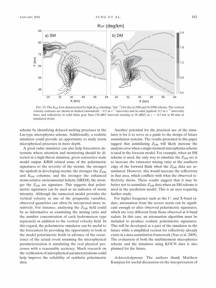
(RFD) region near the surface (Figs. 2c, 10). These
columns are qualitatively similar to those shown in
Figs. 6 and 7 of KR08.
An offset in the centers of the KDP and ZDR columns
was pointed out by Loney et al. (2002) and KR08 in their
observational studies of polarimetric signatures. In the
observations, the KDP column often is found west or
northwest of the ZDR column. A similar offset is ob-
served in the lower midlevels (Figs. 3a,d) in our simula-
tion, while they become collocated at the upper midlevels
(Figs. 3c,f). At the 3-km altitude, the ZDR column is lo-
cated southeast of the updraft core near the reflectivity
hook. This agrees well with the location of the ZDR col-
umn reported in Hubbert et al. (1998). At this level, the
JANUARY 2010 J U N G E T A L . 151

FIG. 1. Reflectivity (thin solid contours and shading), negative perturbation potential temperature (dotted con-
tours at 1.0-K intervals from 21.0 K) and horizontal perturbation wind vectors (plotted every sixth grid point; m s21)
at z 5 250 m for the simulated storm using (left) SM and (right) DM microphysics schemes at (a),(b) 60, (c),(d) 80,
and (e),(f) 100 min. Line AA9 in (f) show the locations of the vertical cross sections to be shown in Fig. 2.
152 J O U R N A L O F A P P L I E D M E T E O R O L O G Y A N D C L I M A T O L O G Y VOLUME 49

KDP column is found at the reflectivity maximum and in
the west and northwest part of the updraft core. At the
4-km altitude, the ZDR column appears as a half-ring
wrapping around the updraft core on the east side (Fig.
3b), while the center of the KDP column is moving to-
ward the updraft core (Fig. 3e). At the 5-km height, the
ZDR and KDP columns are almost collocated with the
updraft core (Figs. 3c,f). No obvious offset in the centers
is found in the SM run (Fig. 4).
The main cause of the offset of the ZDR column from the
updraft core is the presence of hail. From Figs. 3g–i, the
production of qr apparently is strongly related to the up-
draft. Within the updraft, the low-level qr is transported to
the higher level, and qr is also created through in situ
condensation and autoconversion from cloud water; qh is
also produced in the updraft. Large hailstones fall through
the updraft, and small hailstones are carried out of the
updraft while growing and falling in the forward flank
region north of the updraft core. The high-qh region
overlaps with the high qr region in the west-northwest. The
presence of hail reduces the ZDR because the tumbling
nature of the hailstones makes their apparent shape close
to spherical. Therefore, the high ZDR column shows up at
the southeast-to east-side of the updraft.
On the other hand, the KDP is almost transparent to
the hail and is sensitive only to the amount of rainwater.
Therefore, the KDP maximum, high qr region, and up-
draft core are almost collocated.
2) ZDR ARC
The ZDR arc is the low-level signature often observed
at the southern edge of forward flank along the sharp
gradient zone of reflectivity in right-moving supercells
(Ryzhkov et al. 2005; KR08; KR09; Romine et al. 2008).
This is characterized by a horizontally elongated high
ZDR band along the right edge of the forward flank near
the surface and is a quite common feature in supercells,
regardless of season or geographic region. Disdrometer
and polarimetric radar measurements of Schuur et al.
(2001) showed that a very large median volume diameter
is observed in this region. This signature was analyzed in
detail in KR09, where the researchers argued that the size
sorting mechanism, because of strong wind speed and
directional shears, is primarily responsible for this sig-
nature; large drops discharged from the updraft fall into
the region close to the origin, while smaller drops are
advected farther into the forward flank. The rain evapo-
ration is likely another contributing factor modifying the
DSD toward a large Dnr because it selectively depletes
small drops more quickly than larger drops (Rosenfeld
and Ulbrich 2003). At the location of the ZDR arc, the
DSD, initially lacking small drops, loses small drops fast
because of evaporation while falling through dry air in
a shear environment (Milbrandt and Yau 2005a; Dawson
et al. 2010). To properly model such processes respon-
sible for DSD changes, a two- or higher-moment micro-
physics scheme must be used; an SM scheme is not
capable of handling such mechanisms (Fig. 5a).
The modified DSD of rain as a result of the size sorting
can be evaluated easily by examining the mean-mass
diameter Dnr, where Dnr is calculated for the exponen-
tial distribution as
Dnr
5q
rr
air
prrNt
r
� �1/3
, (8)
where rair is the density of air. For an SM scheme, Dnr is
dependent only on qr because Ntr 5 N0rDnr, where N0r is
FIG. 2. Vertical cross sections of simulated (a) ZH (dBZ), (b) ZDR (dB), and (c) KDP (8 km21), along line AA9 shown in Fig. 1h
corresponding to x 5 34.5 km of the simulated supercell storm at 100 min. The 08C isotherms are shown as thick black lines. Deep vertical
columns with high ZDR and KDP values are extended above freezing level at this cross section.
JANUARY 2010 J U N G E T A L . 153

a constant. The DSD directly affects ZDR because ZDR
is proportional to the median diameter of precipitation
particles in the radar resolution volume. The calculated
Dnr for SM and DM is presented in Fig. 5 along with
simulated ZDR.
The ZDR arc signature is well captured by the DM
scheme and polarimetric radar data simulator at a 0.5-km
altitude at 80 min of simulated storm in Fig. 5b. The high
ZDR region along the southern edge of the forward flank
is shallow (;2 km deep), rather narrow, but persistent in
time, quantitatively similar to polarimetric radar obser-
vations of supercell storms, and it shifts slightly toward
the north with height. The arc band becomes weak and
broad above 2 km, practically fading away. The shape
and location of the high ZDR region match the Dnr pat-
tern. The qr pattern, in conjunction with that of Dnr,
designates this area as having a small number of large
drops and lacking small drops. On the other hand, the
FIG. 3. (a)–(c) ZDR (shading; dB) and reflectivity (solid contours at 15-dBZ intervals, starting at 15 dBZ), (d)–(f) KDP (shading; 8 km21)
and perturbation horizontal wind vectors (plotted every other grid point; m s21), and (g)–(i) hail mixing ratio qh (shading; g kg21) and
rain mixing ratio qr (solid contours at 1.5 g kg21 intervals starting at 0.5 g kg21) at (left) 3-, (center) 4-, and (right) 5-km height, at 100 min
of simulated storm. The vertical velocity contours (dotted contours at 10 m s21 intervals starting at 10 m s21) are overlaid on each plot.
154 J O U R N A L O F A P P L I E D M E T E O R O L O G Y A N D C L I M A T O L O G Y VOLUME 49

simulated storm using the SM scheme completely misses
the ZDR arc signature because both Dnr and ZDR are
proportional only to rainwater mixing ratio qr (Fig. 5a).
3) MIDLEVEL ZDR AND rhy RINGS
The midlevel ZDR ring (KR08) refers to the enhanced
ZDR in the shape of a ring occasionally found in the
middle levels. The ZDR ring is sometimes a complete circle
and sometimes just a half-ring. KR08 reported that the
enhanced ZDR region is found always on the right flank of
the updraft when only a half-ring is manifested. In our
simulation, it is usually a half-ring on the right flank of the
updraft at the midlevels and close to a complete ring in the
lower levels.
The half-ZDR ring in Fig. 6b mostly overlaps with the
high Dnr region. The maximum Dnr region is collocated
with the updraft core. The local maxima found on the
south and east sides of the main Dnr core may be ex-
plained by large raindrops falling around the updraft
following a cyclonic circulation (associated with a cy-
clonically rotating updraft; Figs. 3d–f). The missing half
of the ring signature is closely related to the presence of
hail (Fig. 6b). As discussed earlier in section 4b(1), the
presence of hailstones reduces the ZDR values because
their tumbling motion and random orientation make their
apparent shape spherical to radar beams. At the 4-km
altitude, the region with high–hail mixing ratios is located
to the west and northwest of the updraft core. This
weakens the ZDR signature on the left flank of the updraft.
The rhy ring is another midlevel feature with de-
pressed (instead of increased) rhy values in a ring pattern
(KR08). A well-defined rhy ring is seen in Fig. 6d. The
rhy values for pure water and ice are very high but de-
crease when hydrometeors of diverse types are mixed
together. The dotted contours in Fig. 6d show the ratio
of rain–hail mixture to the rain and dry hail total mixing
ratio. High values of this ratio indicate the presence of
three different types, with the mixture being dominant
in the regions of the rhy ring. The low values of the ratio
suggest either pure rain or dry hail is dominant [see
Eq. (2) and section 3b of JZX08 for more details on the
melting ice model used here]. The pattern of this ratio
agrees well with the ring-shaped rhy depression. These
midlevel ZDR and rhy rings are very weak or completely
missing when an SM is used (Figs. 6a,c). The Dnr con-
tours are not shown in Fig. 6a because the maximum Dnr
is smaller than 1.2 mm because of the large intercept
parameter value with SM schemes.
When ice is in a melting phase, the resonance effect due
to Mie scattering can contribute to the reduction of rhy
(Fig. 7a), which occurs when the ratio Dj«j1/2/l ap-
proaches 1 (KR08; KR09), where « is the dielectric con-
stant. For dry hail, rhy slowly decreases with size within
the range shown in Fig. 7a, in which the particle size is
truncated at 42.35 mm. With the given exponential DSD,
large drops have little effect because the number of drops
is very small at that size, although the resonance effect
can be much more significant in very large drops. The rhy
shows a sudden drop at a certain size. Both the charac-
teristic size and maximum amplitude reduction decrease
with increasing water fraction. The size sorting mecha-
nism is also necessary to simulate this signature, so that
the DSD can have a sufficient number of hailstones at the
characteristic size to reduce the total rhy values.
Figure 7b shows the number concentration N(D) at
each particle size D and accumulated rhy from the mini-
mum size up to size D for two selected grid points from the
simulated storm shown in Figs. 6b and 6d. The rain–hail
FIG. 4. (a) As in Fig. 3a and (b) as in Fig. 3d for the SM scheme.
JANUARY 2010 J U N G E T A L . 155

mixture mixing ratio, percentage water fraction, in-
tercept parameter, and total number concentration for
these two grid points are (1.03 g kg21, 51%, 1.49 3
104 m24, 33.893 m23) and (0.995 g kg21, 46%, 1.95 3
105 m24, 208.42 m23). Mixing ratios are similar at these
two points but their intercept parameters differ by an
order of magnitude. When the intercept parameter is
large, N(D) decreases rapidly with size (thick solid gray)
and particles with resonance sizes have very little impact
on accumulated rhy (thick dashed gray). On the contrary,
N(D) decreases slowly when the intercept parameter is
small (solid black) and accumulated rhy exhibits a sudden
reduction near the resonance sizes and slowly increases as
D further increases (dashed black).
We would like to point out that the simulated rhy is
higher than the typically observed values. One source of
difference might be the simplified model of randomly
orientated spheroids for hail and snow used here, which
does not account for the effect of irregular shapes of
natural hydrometeors. The high rhy also may be attrib-
uted partially to our treating each precipitating type
independently when calculating radar reflectivity factor
and combining them afterward [see Eq. (6)] while in the
real atmosphere the radar would see them as a mixture
of irregular shaped, randomly oriented particles. Non-
meteorological effects that can also contribute to the
reduction of rhy, such as noise bias, clutter contamina-
tion, dust, and bugs, are not included in our simulator.
FIG. 5. The ZDR (shading), qr (solid contours at 1.0 g kg21 intervals, starting at 0.5 g kg21),
and mean-mass diameter of raindrops Dnr (dotted black contours at intervals of 0.3 mm,
starting at 0.3 mm) for the (a) SM and (b) DM scheme at z 5 500 m at 80 min of simulated
storm. The ZDR arc structure in the southern edge of the forward flank region agrees well with
the area of the large mean-mass diameter with the DM scheme.
156 J O U R N A L O F A P P L I E D M E T E O R O L O G Y A N D C L I M A T O L O G Y VOLUME 49

These may partially be responsible for the rather high
rhy in our simulation.
To further evaluate the fidelity of our simulator, we
compared the above signatures to those simulated using
the simple simulator developed in J08, where efficiency
was given a high priority when it was developed for data
assimilation purposes. The simulator of J08 is found to
be able to simulate most of the signatures except for the
rhy ring with the DM scheme. The ZDR and KDP values
are somewhat higher than those using a new simulator
because of the choice of the axis ratio there to avoid
numerical integration. The rhy ring could not be simu-
lated correctly because Mie scattering for the ice species
is not included there (Fig. 8).
4) HAIL SIGNATURE IN FORWARD FLANK
DOWNDRAFT
The observed hail signature is characterized by a high
ZH and low ZDR at the lowest radar elevation associated
with hail reaching the ground (KR08). This feature is also
FIG. 6. (a),(b) ZDR (shading), ZH (solid contours at 15-dBZ intervals from 15 dBZ), qh (dotted contours at 2.0 g kg21 intervals from
1.0 g kg21), and Dnr (thick dashed contours at intervals of 0.6 mm, starting at 1.2 mm), and (c),(d) rhy (shading) and the ratio of rain–hail
mixture to the sum of rain and dry hail mixing ratios (dotted contours at 0.1 intervals from 0.2) for the (left) SM and (right) DM scheme at
80 min at z 5 4 km. Ring features are prominent at this level.
JANUARY 2010 J U N G E T A L . 157

called ‘‘ZDR hole’’ (Wakimoto and Bringi 1988), which
often stretches from the surface up to a certain height.
Our simulated storm exhibits depressed ZDR hole sur-
rounded by high ZDR values at the 500-m altitude, where
high hail concentration is present (Fig. 9b). The simulated
ZDR pattern at this altitude is substantially similar to the
observations shown in Fig. 3a of KR08. This hail signa-
ture is also shown in the SM run although it is weak and its
location is shifted to the north (Fig. 9a).
5) KDP FOOT
The KDP foot refers to a downshear elongated high
KDP region developing left of the updraft (Romine et al.
2008). The KDP foot is collocated with the downdraft
region near the surface and is connected to the KDP
column aloft. High KDP values are attributed to the
presence of melting hail in observational studies (Romine
et al. 2008; Bringi et al. 1986; Brandes et al. 1995; Hubbert
FIG. 7. (a) Simulated rhy with size of melting hailstones for the fraction of water, fw 5 0.45
(dotted), 0.65 (solid), and dry hailstone (dashed). (b) The number concentration N(D) (solid)
and accumulated rhy (dashed) for two selected grid points from the simulated storm shown in
Fig. 5 with (the rain–hail mixture mixing ratio, percent fraction of water, intercept parameter,
and total number concentration) 5 (1.03 g kg21, 51%, 1.49 3 104 m24, 33.893 m23; black) and
(0.995 g kg21, 46%, 1.95 3 105 m24, 208.42 m23; thick gray).
158 J O U R N A L O F A P P L I E D M E T E O R O L O G Y A N D C L I M A T O L O G Y VOLUME 49

et al. 1998). The supercell storm with a DM scheme
exhibits all these characteristics of KDP foot in Fig. 2c
and Fig. 10b. The KDP maximum appears in the down-
draft at z 5 500 m in Fig. 10 and is tilted upshear with
height, and linked to the KDP column (Fig. 2c). The KDP
foot structure agrees well with that of the hail mixing
ratio (Fig. 6b). The SM runs produce a similar-shaped
KDP foot to that of the DM runs near the surface but the
KDP values are much too low for the SM case (Fig. 10a).
5. Summary and discussion
In this paper, a synthetic polarimetric radar simulator
based on full T-matrix scattering calculations and ac-
curate formulations for polarimetric radar variables is
developed. The new simulator takes advantage of the
continuous melting ice model developed in JZX08. The
density of the melting ice and dielectric constant are
also allowed to vary continuously. This simulator can
specify any weather radar wavelength and uses up to
three moments of microphysics parameterization (i.e.,
the total number concentrations, mixing ratios, and
reflectivity factors of multiple hydrometeors) as input.
This simulator can simulate the reflectivity of the
horizontal and vertical polarizations (ZH and ZV), dif-
ferential reflectivity (ZDR), specific differential phase
(KDP), and cross-correlation coefficient (rhy), as well as
radial velocity (Vr). These quantities are what will be ob-
served by operational WSR-88D radars after the polari-
metric upgrade and are currently being measured by the
proof-of-concept polarimetric WSR-88D radar (KOUN)
located in Norman, Oklahoma.
The new radar simulator is applied to an idealized
supercell storm simulated using a two- or double-moment
microphysics scheme. The storm with the same config-
urations but using a single-moment microphysics scheme
is created for comparison. The simulated storm using
a DM scheme exhibits unique polarimetric signatures
reported in the literature, including the ZDR and KDP
columns, ZDR arc, midlevel ZDR and rhy rings, hail sig-
nature, and KDP foot. Some of the signatures, mostly
related to the size sorting mechanisms, however, could
not be simulated when an SM scheme was used. These
signatures include the ZDR arc and midlevel ZDR and rhy
rings. These results support that a two- or higher-
moment microphysics scheme must be used to properly
describe these important aspects of thunderstorms.
Properly simulating these processes is also important to
effectively assimilate polarimetric data into numerical
models for initialization purposes.
FIG. 8. As in Fig. 6d, but for simulation using the observation operator of J08. The Mie
scattering effect is not included in this simple version of simulator.
JANUARY 2010 J U N G E T A L . 159

The verification of convective-scale numerical weather
prediction is challenging because most of the model
variables are not directly observed at this scale. Radar
reflectivity has been used to verify the model prediction
for a while. However, reflectivity alone is insufficient to
verify microphysics because many independent vari-
ables and uncertain constants based on many assump-
tions on drop size distributions (DSDs) are involved in
reflectivity calculation. Here, simulated polarimetric
variables can help discriminate against and/or highlight
certain variables from others by using their differential
sensitivity to the water phases. They can be as useful as
reflectivity because they contain additional information
on the DSDs and microphysical processes. As an exam-
ple, JZX08 demonstrated that a realistic radar simulator
could be useful in evaluating the model microphysics
FIG. 9. The hail signature as characterized by high ZH (thin solid contours at 15-dBZ in-
tervals, starting at 15 dBZ) and low ZDR (shading; dB) for the (a) SM and (b) DM scheme at z 5
0.5 km at 70 min of simulated storm. The hail mixing ratio is overlaid in thick dotted contours
at 0.2 g kg21 intervals starting at 0.2 g kg21.
160 J O U R N A L O F A P P L I E D M E T E O R O L O G Y A N D C L I M A T O L O G Y VOLUME 49
scheme by identifying delayed melting processes in the
Lin-type microphysics scheme. Additionally, a realistic
simulator could provide an opportunity to study storm
microphysical processes in more depth.
A good radar simulator can also help forecasters de-
termine where attention and monitoring should be di-
rected in a high-threat situation, given convective-scale
model output. KR08 related some of the polarimetric
signatures to the severity of the storms: the stronger
the updraft in developing storms, the stronger the ZDR
and KDP columns; and the stronger the enhanced
storm-relative environmental helicity (SREH), the stron-
ger the ZDR arc signature. This suggests that polari-
metric signatures can be used as an indicator of storm
intensity. Although the numerical model provides the
vertical velocity as one of the prognostic variables,
observed quantities can often be interpreted more in-
tuitively. For instance, analyzing the ZDR field could
be as informative as examining the mixing ratio and
the number concentration of each hydrometeor type
separately in addition to the vertical velocity field. In
this regard, the polarimetric simulator can be useful to
the forecasters by providing the opportunity to look at
the model polarimetric fields in advance of the occur-
rence of the actual event assuming the microphysical
parameterization is simulating the real physical pro-
cesses with a reasonable accuracy. Much research on
the verification of microphysical parameterizations could
help improve the reliability of synthetic polarimetric
data.
Another potential for the practical use of the simu-
lator is for it to serve as a guide to the design of future
assimilation systems. The results presented in this paper
suggest that assimilating ZDR will likely increase the
analysis error when a single-moment microphysics scheme
is used in the forecast model. For example, when an SM
scheme is used, the only way to simulate the ZDR arc is
to increase the rainwater mixing ratio at the southern
edge of the forward flank when the ZDR data are as-
similated. However, this would increase the reflectivity
in that area, which conflicts with what the observed re-
flectivity shows. These results suggest that it may be
better not to assimilate ZDR data when an SM scheme is
used in the prediction model. This is an area requiring
further study.
For higher frequency such as the C- and X-band ra-
dars, attenuation from the severe storm can be signifi-
cant enough to alter observed polarimetric signatures,
which are very different from those observed at S-band
radars. In this case, an attenuation algorithm must be
included to produce realistic polarimetric signatures.
This will be developed as a part of the simulator in the
future while a simplified version for reflectivity already
exists in a data assimilation framework (Xue et al. 2009).
The evaluation of both the multimoment microphysics
scheme and the simulator using KOUN data is also
planned for the future.
Acknowledgments. The authors thank Matthew
Kumjian for useful discussion on the interpretation of
FIG. 10. The KDP foot characterized by high KDP (shading; 8 km21) for the (a) SM and (b) DM scheme. The vertical
velocity contours are shown in dashed (downdraft; 20.5 m s21 intervals) and in solid (updraft; 0.5 m s21 intervals)
lines, and reflectivity in solid thick gray lines (20-dBZ intervals starting at 20 dBZ) at z 5 0.5 km at 80 min of
simulated storm.
JANUARY 2010 J U N G E T A L . 161

observed polarimetric signature. The authors also thank
Dr. Jason Milbrandt and Daniel Dawson for helping us
to use a multimoment microphysics scheme. The original
T-matrix code was provided by Dr. J. Vivekanandan.
This work was primarily supported by NSF Grants EEC-
0313747 and ATM-0608168. Ming Xue was also sup-
ported by NSF Grants ATM-0530814, ATM-0802888,
ATM-0331594, and ATM-0331756. The computations
were performed at the OU Supercomputing Center for
Education and Research.
REFERENCES
Beard, K. V., R. J. Kubesh, and H. T. Ochs, 1991: Laboratory
measurements of small raindrop distortion. Part I: Axis ratios
and fall behavior. J. Atmos. Sci., 48, 698–710.
Brandes, E. A., 1978: Mesocyclone evolution and tornadogenesis:
Some observations. Mon. Wea. Rev., 106, 995–1011.
——, 1984: Vertical vorticity generation and mesocyclone suste-
nance in tornadic thunderstorms: The observational evidence.
Mon. Wea. Rev., 112, 2253–2269.
——, 1993: Tornadic thunderstorm characteristics determined with
Doppler radar. The Tornado: Its Structure, Dynamics, Pre-
diction and Hazards, Geophys. Monogr., Vol. 79, Amer. Geo-
phys. Union, 143–159.
——, J. Vivekanandan, J. D. Tuttle, and C. J. Kessinger, 1995: A
study of thunderstorm microphysics with multiparameter ra-
dar and aircraft observations. Mon. Wea. Rev., 123, 3129–3143.
——, G. Zhang, and J. Vivekanandan, 2002: Experiments in rain-
fall estimation with a polarimetric radar in a subtropical en-
vironment. J. Appl. Meteor., 41, 674–685.
——, ——, and ——, 2004: Comparison of polarimetric radar drop
size distribution retrieval algorithms. J. Atmos. Oceanic Tech-
nol., 21, 584–598.
Bringi, V. N., R. M. Rasmussen, and J. Vivekanandan, 1986:
Multiparameter radar measurements in Colorado convective
storms. Part I: Graupel melting studies. J. Atmos. Sci., 43,
2545–2563.
Browning, K. A., 1964: Airflow and precipitation trajectories
within severe local storms which travel to the right of the mean
winds. J. Atmos. Sci., 21, 634–639.
——, and R. J. Donaldson, 1963: Airflow and structure of a torna-
dic storm. J. Atmos. Sci., 20, 533–545.
Capsoni, C., M. D’Amico, and R. Nebuloni, 2001: A multiparam-
eter polarimetric radar simulator. J. Atmos. Oceanic Technol.,
18, 1799–1809.
Conway, J. W., and D. S. Zrnic, 1993: A study of embryo pro-
duction and hail growth using dual-Doppler and multipa-
rameter radars. Mon. Wea. Rev., 121, 2511–2528.
Dawson, D. T., II, 2009: Impacts of single- and multi-moment mi-
crophysics on numerical simulations of supercells and torna-
does of the 3 May 1999 Oklahoma tornado outbreak. Ph.D.
dissertation, School of Meteorology, University of Oklahoma,
173 pp.
——, M. Xue, J. A. Milbrandt, M. K. Yau, and G. Zhang, 2007:
Impact of multi-moment microphysics and model resolution
on predicted cold pool and reflectivity intensity and structures
in the Oklahoma tornadic supercell storms of 3 May 1999.
Preprints, 22nd Conf. on Numerical Weather Prediction, Park
City, UT, Amer. Meteor. Soc., 10B.2. [Available online at
http://ams.confex.com/ams/pdfpapers/124706.pdf.]
——, ——, ——, and ——, 2010: Comparison of evaporation and
cold pool development between single-moment and multi-
moment bulk microphysics schemes in idealized simulations of
tornadic thunderstorms. Mon. Wea. Rev., in press.
Doviak, R., and D. Zrnic, 1993: Doppler Radar and Weather Ob-
servations. 2nd ed. Academic Press, 562 pp.
Gilmore, M. S., J. M. Straka, and E. N. Rasmussen, 2004: Pre-
cipitation uncertainty due to variations in precipitation parti-
cle parameters within a simple microphysics scheme. Mon.
Wea. Rev., 132, 2610–2627.
Green, A. V., 1975: An approximation for shape of large raindrops.
J. Appl. Meteor., 14, 1578–1583.
Huang, G.-J., V. N. Bringi, S. van den Heever, and W. Cotton, 2005:
Polarimetirc radar signatures from RAMS microphysics. Pre-
prints, 32nd Int. Conf. on Radar Meteorology, Albuquerque,
NM, Amer. Meteor. Soc., P11R.6. [Available online at http://
ams.confex.com/ams/pdfpapers/96261.pdf.]
Hubbert, J., V. N. Bringi, L. D. Carey, and S. Bolen, 1998: CSU-
CHILL polarimetric radar measurements from a severe hail
storm in eastern Colorado. J. Appl. Meteor., 37, 749–775.
Illingworth, A. J., J. W. F. Goddard, and S. M. Cherry, 1987: Po-
larization radar studies of precipitation development in con-
vective storms. Quart. J. Roy. Meteor. Soc., 113, 469–489.
Jung, Y., 2008: State and parameter estimation using polarimetric
radar data and an ensemble Kalman filter. Ph.D. dissertation,
School of Meteorology, University of Oklahoma, 209 pp.
——, G. Zhang, and M. Xue, 2008a: Assimilation of simulated
polarimetric radar data for a convective storm using ensemble
Kalman filter. Part I: Observation operators for reflectivity
and polarimetric variables. Mon. Wea. Rev., 136, 2228–2245.
——, M. Xue, G. Zhang, and J. Straka, 2008b: Assimilation of
simulated polarimetric radar data for a convective storm using
ensemble Kalman filter. Part II: Impact of polarimetric data
on storm analysis. Mon. Wea. Rev., 136, 2246–2260.
Klemp, J. B., and R. B. Wilhelmson, 1978: Simulations of right- and
left-moving thunderstorms produced through storm splitting.
J. Atmos. Sci., 35, 1097–1110.
——, and M. L. Weisman, 1983: The dependence of convective
precipitation patterns on vertical wind shear. Preprints, 21st
Conf. on Radar Meteorology, Edmonton, AB, Canada, Amer.
Meteor. Soc., 44–49.
——, R. B. Wilhelmson, and P. S. Ray, 1981: Observed and nu-
merically simulated structure of a mature supercell thunder-
storm. J. Atmos. Sci., 38, 1558–1580.
Knight, N. C., 1986: Hailstone shape factor and its relation to
radar interpretation of hail. J. Climate Appl. Meteor., 25,
1956–1958.
Kumjian, M. R., and A. V. Ryzhkov, 2008: Polarimetric signatures
in supercell thunderstorms. J. Appl. Meteor. Climatol., 47,
1940–1961.
——, and ——, 2009: Storm-relative helicity revealed from polar-
imetric radar measurements. J. Atmos. Sci., 66, 667–685.
Lemon, L. R., and C. A. Doswell, 1979: Severe thunderstorm
evolution and mesocyclone structure as related to tornado-
genesis. Mon. Wea. Rev., 107, 1184–1197.
Lin, Y.-L., R. D. Farley, and H. D. Orville, 1983: Bulk parame-
terization of the snow field in a cloud model. J. Climate Appl.
Meteor., 22, 1065–1092.
Loney, M. L., D. S. Zrnic, J. M. Straka, and A. V. Ryzhkov, 2002:
Enhanced polarimetric radar signatures above the melting
level in a supercell storm. J. Appl. Meteor., 41, 1179–1194.
Marshall, J. S., and W. M. Palmer, 1948: The distribution of rain-
drops with size. J. Meteor., 5, 165–166.
162 J O U R N A L O F A P P L I E D M E T E O R O L O G Y A N D C L I M A T O L O G Y VOLUME 49
Marwitz, J. D., 1972: The structure and motion of severe hail-
storms. Part I: Supercell storms. J. Appl. Meteor., 11, 166–179.
Meyers, M. P., R. L. Walko, J. R. Harrintong, and W. R. Cotton,
1997: New RAMS cloud microphysics parameterization. Part
II: The two-moment scheme. Atmos. Res., 45, 3–39.
Milbrandt, J. A., and M. K. Yau, 2005a: A multi-moment bulk
microphysics parameterization. Part I: Analysis of the role of
the spectral shape parameter. J. Atmos. Sci., 62, 3051–3064.
——, and ——, 2005b: A multi-moment bulk microphysics pa-
rameterization. Part II: A proposed three-moment closure and
scheme description. J. Atmos. Sci., 62, 3065–3081.
——, and ——, 2006: A multi-moment bulk microphysics param-
eterization. Part IV: Sensitivity experiments. J. Atmos. Sci., 63,
3137–3159.
Musil, D. J., A. J. Heymsfield, and P. L. Smith, 1986: Microphysical
characteristics of a well-developed weak echo region in a High
Plains supercell thunderstorm. J. Climate Appl. Meteor., 25,
1037–1051.
Pfeifer, M., G. C. Craig, M. Hagan, and C. Keil, 2008: A polari-
metric radar forward operator for model evaluation. J. Appl.
Meteor. Climatol., 47, 3202–3220.
Ray, P. S., B. Johnson, K. W. Johnson, J. S. Bradberry, J. J. Stephens,
K. K. Wagner, R. B. Wilhelmson, and J. B. Klemp, 1981: The
morphology of severe tornadic storms on 20 May 1977. J. Atmos.
Sci., 38, 1643–1663.
Romine, G. S., D. W. Burgess, and R. B. Wilhelmson, 2008: A dual-
polarization-radar-based assessment of the 8 May 2003
Oklahoma City area tornadic supercell. Mon. Wea. Rev., 136,
2849–2870.
Rosenfeld, D., and C. W. Ulbrich, 2003: Cloud microphysical
properties, processes, and rainfall estimation opportunities.
Radar and Atmospheric Science: A Collection of Essays in
Honor of David Atlas, Meteor. Monogr., No. 52, Amer.
Meteor. Soc., 237–258.
Rotunno, R., 1981: On the evolution of thunderstorm rotation.
Mon. Wea. Rev., 109, 171–180.
Ryzhkov, A. V., 2001: Interpretation of polarimetric radar co-
variance matrix for meteorological scatterers: Theoretical
analysis. J. Atmos. Oceanic Technol., 18, 315–328.
——, D. S. Zrnic, and B. A. Gordon, 1998: Polarimetric method for
ice water content determination. J. Appl. Meteor., 37, 125–134.
——, T. J. Schuur, D. W. Burgess, and D. S. Zrnic, 2005: Polari-
metric tornado detection. J. Appl. Meteor., 44, 557–570.
Schuur, T. J., A. V. Ryzhkov, D. S. Zrnic, and M. Schonhuber,
2001: Drop size distributions measured by a 2D video dis-
drometer: Comparison with dual-polarization radar data.
J. Appl. Meteor., 40, 1019–1034.
Tong, M., and M. Xue, 2005: Ensemble Kalman filter assimilation
of Doppler radar data with a compressible nonhydrostatic
model: OSS experiments. Mon. Wea. Rev., 133, 1789–1807.
Vivekanandan, J., W. M. Adams, and V. N. Bringi, 1991: Rigorous
approach to polarimetric radar modeling of hydrometeor
orientation distributions. J. Appl. Meteor., 30, 1053–1063.
——, V. N. Bringi, M. Hagen, and G. Zhang, 1994: Polarimetric
radar studies of atmospheric ice particles. IEEE Trans. Geo-
sci. Remote Sens., 32, 1–10.
Wakimoto, R. M., and V. N. Bringi, 1988: Dual-polarization ob-
servations of microbursts associated with intense convection:
The 20 July storm during the MIST Project. Mon. Wea. Rev.,
116, 1521–1539.
Waldvogel, A., 1974: The N0-jump of raindrop spectra. J. Atmos.
Sci., 31, 1067–1078.
Walko, R. L., W. R. Cotton, M. P. Meyers, and J. L. Harrington,
1995: New RAMS cloud microphysics parameterization. Part I:
The single-moment scheme. Atmos. Res., 38, 29–62.
Waterman, P. C., 1969: Scattering by dielectric obstacles. Alta
Freq., 38 (speciale), 348–352.
Weisman, M. L., and J. B. Klemp, 1982: The dependence of nu-
merically simulated convective storms on vertical wind shear
and buoyancy. Mon. Wea. Rev., 110, 504–520.
Xue, M., 2000: High-order monotonic numerical diffusion and
smoothing. Mon. Wea. Rev., 128, 2853–2864.
——, K. K. Droegemeier, and V. Wong, 2000: The Advanced Re-
gional Prediction System (ARPS) - A multiscale nonhydrostatic
atmospheric simulation and prediction tool. Part I: Model dy-
namics and verification. Meteor. Atmos. Phys., 75, 161–193.
——, and Coauthors, 2001: The Advanced Regional Prediction
System (ARPS) - A multiscale nonhydrostatic atmospheric
simulation and prediction tool. Part II: Model physics and
applications. Meteor. Atmos. Phys., 76, 143–165.
——, D.-H. Wang, J.-D. Gao, K. Brewster, and K. K. Droegemeier,
2003: The Advanced Regional Prediction System (ARPS),
storm-scale numerical weather prediction and data assimila-
tion. Meteor. Atmos. Phys., 82, 139–170.
——, M. Tong, and K. K. Droegemeier, 2006: An OSSE framework
based on the ensemble square root Kalman filter for evaluating
impact of data from radar networks on thunderstorm analysis
and forecast. J. Atmos. Oceanic Technol., 23, 46–66.
——, Y. Jung, and G. Zhang, 2007: Error modeling of simulated
reflectivity observations for ensemble Kalman filter data as-
similation of convective storms. Geophys. Res. Lett., 34,L10802, doi:10.1029/2007GL029945.
——, M. Tong, and G. Zhang, 2009: Simultaneous state estimation
and attenuation correction for thunderstorms with radar data
using an ensemble Kalman filter: Tests with simulated data.
Quart. J. Roy. Meteor. Soc., 135, 1409–1423.
Zhang, G., J. Vivekanandan, and E. Brandes, 2001: A method for
estimating rain rate and drop size distribution from polari-
metric radar measurements. IEEE Trans. Geosci. Remote
Sens., 39, 830–841.
JANUARY 2010 J U N G E T A L . 163
Top Related