


Languages
Pages
Legal


Journal of Physics Conference Series
OPEN ACCESS
Simulating Dynamic Stall in a 2D VAWT Modelingstrategy verification and validation with ParticleImage Velocimetry dataTo cite this article C J Simatildeo Ferreira et al 2007 J Phys Conf Ser 75 012023
View the article online for updates and enhancements
You may also likeOverview and Design of self-acting pitchcontrol mechanism for vertical axis windturbine using multi body simulationapproachPrasad Chougule and Soslashren Nielsen
-
Effects of Solidity on AerodynamicPerformance of H-Type Vertical Axis WindTurbineChangping Liang Deke Xi Sen Zhang etal
-
Integrated design of a semi-submersiblefloating vertical axis wind turbine (VAWT)with active blade pitch controlFons Huijs Ebert Vlasveld Maeumll Gormandet al
-
This content was downloaded from IP address 19616830178 on 02012022 at 1845
Simulating Dynamic Stall in a 2D VAWT
Modeling strategy verification and validation with
Particle Image Velocimetry data
CJ Simao Ferreira H Bijl G van Bussel G van Kuik
DUWIND- Delft University Wind Energy Research Institute Kluyverweg 1 2629 HS Delft NL
E-mail cjsimaoferreiratudelftnl
Abstract
The implementation of wind energy conversion systems in the built environment renewedthe interest and the research on Vertical Axis Wind Turbines (VAWT) which in this applicationpresent several advantages over Horizontal Axis Wind Turbines (HAWT) The VAWT has aninherent unsteady aerodynamic behavior due to the variation of angle of attack with the angle ofrotation perceived velocity and consequentially Reynolds number The phenomenon of dynamicstall is then an intrinsic effect of the operation of a Vertical Axis Wind Turbine at low tip speedratios having a significant impact in both loads and power
The complexity of the unsteady aerodynamics of the VAWT makes it extremely attractiveto be analyzed using Computational Fluid Dynamics (CFD) models where an approximationof the continuity and momentum equations of the Navier-Stokes equations set is solved
The complexity of the problem and the need for new design approaches for VAWT for thebuilt environment has driven the authors of this work to focus the research of CFD modelingof VAWT on
bullcomparing the results between commonly used turbulence models URANS (Spalart-Allmaras and k-ǫ) and large eddy models (Large Eddy Simulation and Detached EddySimulation)
bullverifying the sensitivity of the model to its grid refinement (space and time)bullevaluating the suitability of using Particle Image Velocimetry (PIV) experimental data formodel validation
The 2D model created represents the middle section of a single bladed VAWT with infiniteaspect ratio The model simulates the experimental work of flow field measurement usingParticle Image Velocimetry by Simao Ferreira et al [1] for a single bladed VAWT
The results show the suitability of the PIV data for the validation of the model the needfor accurate simulation of the large eddies and the sensitivity of the model to grid refinement
Nomenclature
c airfoilblade chord [m]CN normal force [-]CT tangential force [-]D rotor diameter [m]k reduced frequency [-]R rotor radius [m]
The Science of Making Torque from Wind IOP PublishingJournal of Physics Conference Series 75 (2007) 012023 doi1010881742-6596751012023
ccopy 2007 IOP Publishing Ltd 1
Re Reynolds number [-]Uinfin Unperturbed velocity [ms]DES Detached Eddy SimulationLES Large Eddy SimulationRANS Reynolds-Averaged Navier-StokesURANS Unsteady Reynolds-Averaged Navier-Stokes)α angle of attack []θ azimuth angle []ω angular velocity of the rotor frequency [rads]Ω vorticity [sminus1]Γ circulation [m2s]ρ density of the fluid [kgm3]microΓ average value of circulation [m2s]
1 Introduction
The increasing awareness of the need for environmentally sustainable housing and cities hasdriven the promotion of wind energy conversion systems for the built environment One ofthe results of the development of solutions for the built environment is the reappearance ofVertical Axis Wind Turbines (VAWTs) In the built environment the VAWT presents severaladvantages over the more common Horizontal Axis Wind Turbines (HAWTs) namely its lowsound emission (consequence of its operation at lower tip speed ratios) better esthetics due toits three-dimensionality its insensitivity to yaw wind direction and its increased power outputin skewed flow (see Mertens et al [2] and Simao Ferreira et al [3])
The phenomenon of dynamic stall is an inherent effect of the operation of a VAWT at low tipspeed ratios (λ) The presence of dynamic stall has significant impact on both load and power
Modeling the VAWT in dynamic stall presents five immediate challenges
bull The unsteady component of the flow requires a time accurate model adding an extradimension (time) to the numerical grid
bull The geometry of the rotor does not allow for important spatialtime grid simplifications tobe applied (example moving reference frames or radial symmetry)
bull The large amount of shed vorticity implies that the model could be sensitive to numericaldissipation
bull The geometry of a Vertical Axis Wind Turbine results in blade-vortex interaction at thedownwind passage of the blade between the blade and the shed vorticity that was generatedat the upwind passage This means that the development of the shed vorticity must becorrectly modeled inside the entire rotor diameter in order to avoid numerical dissipationthe spatial resolution of the grid must be very fine not only in the immediate vicinity of theblades but over the entire rotor
bull The variation of angle of attack of the blade with azimuth angle implies a varyingrelationdominance between lift and drag force on the blade (resulting in instants during therotation where the VAWT is actually being decelerated because only drag force is present)The correct use of a turbulence model and near-wall models is essential in these situationsThis is particulary important at low tip speed ratios where the power output of the VAWTis negative (for a certain range of λ) the performance at low tip speed ratios is highlyimportant for start-up behavior one of the disadvantages usually associated with VAWT
This numerical model aims at simulating the experimental work by Simao Ferreira et al [1]forconditions of Re = 50000 and tip speed ratio λ = 2 continuing the work presented in [4]
The Science of Making Torque from Wind IOP PublishingJournal of Physics Conference Series 75 (2007) 012023 doi1010881742-6596751012023
2
Contrary to the previous attempts to model the VAWT using CFD (see Hansen et al [5] Allet et al [6] Paraschivoiu et al [7] Paraschivoiu et al [8] and Paraschivoiu [9]) the validationof the results is achieved not by comparing the load on the blades but by comparing the vorticityin the rotor area This work aims also at demonstrating the suitability of PIV data for validationof numerical models for this specific problem
The results of the simulations show the impact of choice of turbulence model and gridrefinement
2 Model geometry and computational grid
The geometry of the model is a 2D representation of the experimental setup of Simao Ferreira etal [1] The CFD grid presents a slight discrepancy later discovered between the location of theairfoil in relation to the radial direction used in the experiment further calculations showed thisdiscrepancy to be negligible in validation of the results and its implications The modelrsquos wallboundary conditions consists of two walls spaced 125m apart where a 04m diameter single-bladed Darrieus VAWT is placed The rotor is represented by an 005m chord NACA0015
airfoil and the 005m rotor axis The rotor axis is placed over the symmetry position of the windtunnel The inlet and outlet boundary conditions are placed respectively 10D upwind and 14Ddownwind of the rotor allowing a full development of the wake
The model comprises a 2D spatial grid simulating the conditions at the middle cross-section ofthe experimental setup The grid is composed of four non-conformal sub-grids each a structuredgrid of quadrilateral elements Figure 1 presents a diagram of the shape and location of eachsub-grid and the wall boundary conditions representing the airfoilblade wind tunnel walls androtor axis (the flow inlet and outlet boundary conditions are not represented)
=0deg
=180deg
=270deg
Figure 1 Diagram of the model geome-try sub-grid distribution and boundary con-ditions
The use of moving sub-grids is necessary due to the movement of the rotor elements Thus thesub-grids Rotor Diameter Blade sub-grid I and Blade sub-grid II rotate with an angular velocityω = 75rads while the sub-grid Wind Tunnel remains fixed The option of dividing the rotorspace in three non-conformal sub-grids allows the use of a structured grid without compromisingits quality or requiring a large mesh with over refinement in areas of lower importance Aquadrilateral structured grid also allows easier control of the refinement of the grid this aspectis crucial in the present work since the sensitivity to the refinement of the space grid is evaluated
The most refined sub-grid is Blade sub-grid I which defines the geometry of the airfoil andits immediate wake development flow region The reference fine grid comprises 3305 nodes overthe airfoil surface where the height of the first row of cells is set at a distance to the wall of
The Science of Making Torque from Wind IOP PublishingJournal of Physics Conference Series 75 (2007) 012023 doi1010881742-6596751012023
3
002c to (y+asymp 1 when θ = 90 kminus ǫ model) The total model size comprises approx 16lowast106
cells
3 Simulated flow conditions
The simulation aimed at representing the flow conditions of the experimental work for λ = 2 andincoming flow Uinfin = 75ms The level of unsteadiness is determined by the reduced frequencyk defined as k = ωc2V where ω is the angular frequency of the unsteadiness c is the bladersquoschord and V is the velocity of the blade In this experiment due to the variation of V withrotation angle k was defined as k = ωc(2λVinfin) = ωc(2ωR) = c(2R) where λ is the tipspeed ratio and R is the radius of rotation For this experimental work k = 0125 placing thework in the unsteady aerodynamics region
Due to the importance of the induction of the rotor it is necessary to perform a simulationfor several rotations until a fully developed wake is present All values presented in this paperrelate to the revolutions of the rotor after a periodic post-transient solution is found
4 Validation of the results of different turbulence models
Figure 2 PIV experimentaldata of the evolution of thecirculation of leading edgeseparated vortex for λ = 2 at90 108 133 and 158)
Four different turbulence models where used in this work complementing the analysis witha Laminar model by Simao Ferreira et al [4] two URANS (Spallart-Almaras and k-ǫ) and twolarge eddy models (DES and LES )
The simulations results are validated against the experimental results of Simao Ferreira etal [1] for the case of λ = 2 These results of which Figures 2 and 3 are an example show thatthe flow is characterized by the shedding to the flow of strong vortices this shedding of vorticityis located
bull at the leading edge resulting of a leading edge separation where the clockwise vorticesdetach from the surface
bull at the trailing edge where a wake is formed from the pressure side boundary layer andthe boundary layer developed in the suction side after the point of leading edge separation-reattachment this wake experiences a roll up due to the strong vorticity
The Science of Making Torque from Wind IOP PublishingJournal of Physics Conference Series 75 (2007) 012023 doi1010881742-6596751012023
4
Figure 3 PIV experimen-tal data of the evolution ofthe counter-clockwise vorticityshed after the roll-up of thetrailing edge vorticity
The validation of the simulations compares the vorticity field in the vicinity of the airfoil attwo azimuthal angles θ = 90 and θ = 120 the choice of these two moments of the rotationis driven by the development of the vorticity shed from the leading edge and the wake at thetrailing edge Taking into account the experimental results the two azimuthal positions define
bull at θ = 90 the vorticity shed at the leading edge has rolled in a large conglomerate of smallvortices in an region one chord length yet the wake at the trailing edge has not yet startedto roll up nor moving over the suction surface
bull at θ = 120 the wake shed at the trailing edge has rolled up and the main counter-clockwisevorticity is over the last quarter of the suction side of the airfoil between the surface andthe leading edge shed vorticity which as started to be convected away from the airfoil
41 URANS models
Unsteady Reynolds-Averaged Navier-Stokes aims at reducing the computational effort by solvingthe Reynolds averaged form of the Navier-Stokes equations (see Bredberg [10]) however requiringthe modeling of the Reynolds stresses originated from the averaging method In the rangeof possible models are eddy-viscosity models which assume that the Reynolds stresses can beestimated by a relation of the eddy viscosity νt and the velocity spatial derivatives In this worktwo of the most popular URANS eddy viscosity models are used the one-equation Spallart-
Almaras (S-A) and the two-equations k-ǫ model The S-A used is the implementation in theCFD package Fluent (see reference [11]) of the model proposed by Sparllat and Almaras [12]The k-ǫ model is the standard implementation in Fluent [11] referred as Standard k-ǫ
Previous attempts on the simulation of 2D VAWT flow (see Hansen et al [5] Allet et al [6] Paraschivoiu et al [7] Paraschivoiu et al [8] and Paraschivoiu [9])) have resorted to theseor similar models the results presented in this paper using URANS are thus a link betweenprevious research and the application of more complex models such as LES and DES
Figures 4 and 5 show the vorticity field in the vicinity of the airfoil at θ = 90 and θ = 120Comparing with the experimental results the S-A model underestimates the generation andshedding of vorticity at the leading edge (in the simulation the leading edge shed vorticityis only located in the first half of the airfoil while experimental results show it covering theentire airfoil length - Figure 2) it is also unable to predict the roll-up of the trailing edge shedvorticity clearly seen in the experimental work (Figure 3) even at θ = 120 The k-ǫ model(Figures 6 and 7) although more computationally expensive is also not able to predict thesetwo main phenomena of the flow field The option of both models of simulating all scales ofturbulence based on the Boussinesq hypothesis of isotropy of the turbulence clearly proved to be
The Science of Making Torque from Wind IOP PublishingJournal of Physics Conference Series 75 (2007) 012023 doi1010881742-6596751012023
5
Figure 4 Vorticity field at θ = 90 Spalart-
Allmaras model
Figure 5 Vorticity field at θ = 120Spalart-Allmaras model
insufficient for the dominant large scales of the flow field The verification of time grid refinement(with the S-A model) lead to two observations the refinement did not produce any significantimprovement in the prediction of the vorticity shed phenomena and a time step of ∆t = 14ωis recommended as maximum time step for a relevant simulation
Figure 6 Vorticity field at θ = 90 k minus ǫmodel
Figure 7 Vorticity field at θ = 120 k minus ǫmodel
The Science of Making Torque from Wind IOP PublishingJournal of Physics Conference Series 75 (2007) 012023 doi1010881742-6596751012023
6
42 LES
The Large Eddy Simulations used is the standard model implemented in Fluent [11] for 2D3Dsimulation Contrary to URANS in LES the equations are not Reynolds-averaged in time butare space filtered (averaged in volume) This operation implies an increase of the computationalrequirements but reduces the turbulence modeling to only the sub-grid scale (SGS model)solving the larger scales of turbulence The SGS model used is the Smagorinsky-Lilly model [11]which is a one equation eddy-viscosity model One of current limitations of LES is itswall treatment where the SGS model is commonly applied (see Spalart [13]) The requiredrefinement of the grid at the wall for a correct simulation of all the scales using LES is still toocomputationally expensive (although one might argue that for a 2D model at moderate Reynoldssome cases are feasible) Attempts to model unsteady airfoil flows with LES (Dahlstrom etal [14]) have shown the feasibility of using LES but raised some challenges regarding the choiceof SGS models and artificial unsteadiness
Figures 8 and 9 show the vorticity distribution around the airfoil for θ = 90 and θ = 120In this simulation the large shedding of leading edge vorticity and the roll-up of the trailingedge wake are simulated (a clear improvement over the URANS model) yet the location ofthe vorticity shed at the leading edge covers a larger area than what was observed in theexperimental results and the roll-up of the trailing edge wake occurs too early in the rotationin the experiments the roll-up of the trailing edge wake starts at θ = 120 (Figure 3) while inthe simulation it can already be seen at θ = 90 (Figure 8)
Figure 8 Vorticity field at θ = 90 Large
Eddy Simulation
Figure 9 Vorticity field at θ = 120 Large
Eddy Simulation
43 DES
Detached-Eddy Simulations used is as implemented in Fluent in 2D3D formulation a hybridmethod of LES and URANS where the wall region is modeled with a URANS model and theouter region with LES the motivation for using DES is the high cost of LES in the boundarylayer region In the present work an S-A model is used for the wall regionlsquo[11]
Figures 10 and 11 show the vorticity distribution around the airfoil for θ = 90 and θ = 120Of all the models used the DES simulations present the results best agreeing with experiments
The Science of Making Torque from Wind IOP PublishingJournal of Physics Conference Series 75 (2007) 012023 doi1010881742-6596751012023
7
the region and location of the turbulence and the phase of roll up of the trailing edge wake areas experimentally observed
The reason for the improvement in relation to the LES can only be accounted by a morecorrect modelling of the wall region even when using a single equation S-A model implying thatthe y+
asymp 1 scale is still too course for an LES simulation Yet the influence of grid refinementin DES and what it implies in the validity of the model can pose a challenge (see Spalart [15])Results of verification of grid sensitivity shall be presented further on this paper
Figure 10 Vorticity field at θ = 90Detached Eddy Simulation
Figure 11 Vorticity field at θ = 120Detached Eddy Simulation
5 Comparison of force simulation
The models have until now been analyzed by comparing the evolution of the shed vorticity withexperimental observations The values of tangential and normal force 1 will now be comparedin Figures 121314 and 15 Three main differences are visible between the URANS models andthe large eddy models DES and LES
bull a non-zero value of normal force at θ = 0 for both URANS models thus representing alarge value of lift at a zero geometric angle of attack in both the DES and LES modelsthe value of the force is zero
bull the azimuthal location of the maxima of tangential and normal forces in the DES andLES models both tangential and normal forces reach a maximum at lower values of θ (incompared with the URANS models) followed by an almost linear decrease with θ thefailure of the URANS models to capture this effect might lay on their inability to correctlymodel the development of vorticity around the airfoil
bull the level of unsteadiness of the forces the DES and LES present large oscillations in theforces at frequencies higher than the frequency of rotation of the turbine this might be aresult of the shedding of strong small vortices in the DES and LES as opposed to a single
1 Tangential force is considered in the direction of rotation of the blade and normal force in the radial direction
The Science of Making Torque from Wind IOP PublishingJournal of Physics Conference Series 75 (2007) 012023 doi1010881742-6596751012023
8
continuous vortex in the URANS models yet numerical convergence effects can also be inthe origin of these fluctuations
0 50 100 150 200 250 300 350minus4
minus2
0
2
4
6
8
θ (deg)
F1
2ρλ2U2
infinc
Normal ForceTangential Force
Figure 12 Tangential and Normal forcein the blade SA model ∆t = 12ωInstantaneous values over three rotations
0 50 100 150 200 250 300 350minus4
minus2
0
2
4
6
8
θ (deg)
F1
2ρλ2U2
infinc
Normal ForceTangential Force
Figure 13 Tangential and Normal forcein the blade k minus ǫ model ∆t = 12ωInstantaneous values over three rotations
0 50 100 150 200 250 300 350minus4
minus2
0
2
4
6
8
θ (deg)
F1
2ρλ2U2
infinc
Normal ForceTangential Force
Figure 14 Tangential and Normal force inthe blade DES ∆t = 14ω Instantaneousvalues over five rotations
0 50 100 150 200 250 300 350minus4
minus2
0
2
4
6
8
θ (deg)
F1
2ρλ2U2
infinc
Normal ForceTangential Force
Figure 15 Tangential and Normal forcein the blade LES model ∆t = 14ωInstantaneous values over four rotations
6 Verification to grid sensitivity
The work of Simao Ferreira et al [4] presented an evaluation of the effect of space and timegrid refinementcoarsening for the case of a Laminar model such evaluation showed a highsensitivity of the results to the refinement of the grid Yet the DES model has proved to be amore suitable simulation tool thus in this section we shall evaluate the robustness of the DES
simulation towards grid refinement
61 Time grid refinement
In the reference simulation a time step ∆t = 14ωminus1 is used The analysis now presentedcompares this simulation with two other with the same initial conditions but time steps
The Science of Making Torque from Wind IOP PublishingJournal of Physics Conference Series 75 (2007) 012023 doi1010881742-6596751012023
9
∆t = 18ωminus1 and ∆t = 116ωminus1Figures 16 and 17 present the vorticity distribution at θ = 90 Similarly to what it was
observed by Simao Ferreira et al [4] with a Laminar model also for the DES model the firstrefinement of the time step (∆t = 18ωminus1) results in a overgeneration of the vorticity and anearly roll-up of the wake at the trailing edge yet the second refinement (∆t = 116ωminus1) doesnot consecutively generate another increase in fact the differences between the two results areminimal and in what is expected in relation to the randomness of the flow This interpretationof the results is also confirmed by the simulated force values (Figure 18) The DES simulationappears to be less sensitive to time grid refinement at this magnitude of step size
Figure 16 Vorticity field at θ = 90 ∆t =18ωminus1
Figure 17 Vorticity field at θ = 90 ∆t =116ωminus1
0 20 40 60 80 100 120 140 160 180minus2
minus1
0
1
2
3
4
5
6
7
8
θ (deg)
F1
2ρλ2U2
infinc
∆ t=14degωminus1
∆ t=18degωminus1
∆ t=116degωminus1
Figure 18 Effect on tangential and normalforce of change of the time grid refinement
62 Space grid refinement
In the work of Simao Ferreira et al [4] the space grid coarsening applied on the Laminar modelresulted in an over generation of vorticity and an earlier roll-up of the trailing edge wake at
The Science of Making Torque from Wind IOP PublishingJournal of Physics Conference Series 75 (2007) 012023 doi1010881742-6596751012023
10
θ = 90 In the current work using a DES model two simulations where performed with coarserspace meshes (x and y) only Blade sub-grid I was coarsened in the first case by quadruplingthe cell area (4∆A doubling height and width) and in the second case by sixteenfold (16∆Aquadrupling height and width)
The results showed in Figures 19 20 and 21 shows that the overgeneration of vorticity andis also present when using a DES model however the variation is not as large as observed inthe laminar model and the effect on the force is small
Figure 19 Vorticity field at θ = 90 ∆t =025ω 2 times coarser grid
Figure 20 Vorticity field at θ = 90 ∆t =025ω
0 20 40 60 80 100 120 140 160 180minus2
minus1
0
1
2
3
4
5
6
7
8
θ (deg)
F1
2ρλ2U2
infinc
∆ Agrid
4∆ Agrid
16∆ Agrid
Figure 21 Effect on tangential and normalforce of change of the space grid refinement
0 20 40 60 80 100 120 140 160 180minus2
minus1
0
1
2
3
4
5
6
7
8
θ (deg)
F1
2ρλ2U2
infinc
∆ t=14degωminus1 N iter
∆ t=14degωminus1 2N iter
∆ t=18degωminus1 N iter
Figure 22 The effect of convergence ontangential and normal force of change of theconvergence iteration
The Science of Making Torque from Wind IOP PublishingJournal of Physics Conference Series 75 (2007) 012023 doi1010881742-6596751012023
11
7 Verification convergence error
The oscillations observed in the force output at frequencies much higher than the rotationalfrequency can have two origins
bull a real physical behavior resulting from the continuous shedding of strong small vortices overthe surface and at the trailing edge
bull a numerical convergence problem where for each time step the solution converges slightlyfaster or slower thus undershooting or overshooting the real value
To observe the validity of the later three simulations of a half rotation starting at the sameinitial condition are compared (Figure 22) The three solutions encompass
bull the reference model with ∆t = 14ωminus1 and N iterations per time step
bull a second model with ∆t = 14ωminus1 and 2N iterations per time step
bull a time refined model with ∆t = 18ωminus1 and N iterations per time step
The results do not present any large change on the amount of high frequency oscillations onthe force curve with the main difference between the curves occurring past the roll up of thetrailing edge vorticity at θ gt 90 The comparison does not allow us to draw any conclusionregarding the effect of convergence and more research is required
8 Conclusions
The results demonstrate the influence of different turbulence models on the accuracy of theprediction of dynamic stall development on a VAWT Of the models analyzed the Detached Eddy
Simulation turbulence model presented the results closest to experiments The DES model isnot only able to predict the generation and shedding of vorticity and itrsquos convection it also showsan acceptable sensitivity to grid refinement (both space and time) thus making it suitable forsimulations where validation data is limited or non existent URANS models proved insufficientdue to their inability of correctly modeling the large eddies The LES performed worse thanthan the DES model probably due to a less accurate modeling of the wall region
The high frequency (in comparison to the rotational frequency) oscillations of the forceson the airfoil might indicate a numerical oscillation of the convergence of the solution in eachtime step Simulations aimed at testing this hypothesis did not reach any final conclusionsince the differences between the various grid refinements are in the range of randomness of thesimulation but prove the need for a experimental study of the time development of forces andpossible frequency analysis
The numerical work proves the usefulness of velocity data (in this case acquired with PIV) forvalidation The visualization of the shedding and convection of the vorticity (in particular thelocation of the leading edge vorticity and the moment of roll up of the trailing edge vorticity)prove to be more specific for validation than the comparison of the force on the blade insimulations with varying grid refinement the simulations presented different behaviors of theflow field clearly identifiable in comparison with experimental data Yet the result of theintegral forces on the airfoil did not present differences outside the uncertainty range associatedwith the randomness of the flow
Future research will focus on developing modeling guidelines applying DES focusing on
bull limiting the uncertainty associated with grid refinement
bull testing the different turbulence sub-models and wall treatment models
bull applying simulation for performance evaluation of different airfoil shapes (camber andthickness effects)
bull analyze the influence of wall models with special focus on the calculation of friction drag
The Science of Making Torque from Wind IOP PublishingJournal of Physics Conference Series 75 (2007) 012023 doi1010881742-6596751012023
12
9 Acknowledgments
The authors would like to thank Dr van Zuijlen (DUWIND) for his insightful help and remarks
10 Bibliography[1] CJ Simao Ferreira G van Bussel and G van Kuik 2D PIV visualization of dynamic stall on a vertical axis
wind turbine In 45th AIAA Aerospace Sciences Meeting and Exhibit ASME Wind Energy Symposium2007
[2] S Mertens G van Kuik and G van Bussel Performance of a H-Darrieus in the skewed flow on a roofJournal of Solar Energy Engineering 125433ndash440 2003
[3] CJ Simao Ferreira G van Bussel and G van Kuik Wind tunnel hotwire measurements flow visualizationand thrust measurement of a VAWT in skew In 44th AIAA Aerospace Sciences Meeting and ExhibitASME Wind Energy Symposium 2006
[4] CJ Simao Ferreira G van Bussel and G van Kuik 2D CFD simulation of dynamic stall on a Vertical AxisWind Turbine verification and validation with PIV measurements In 45th AIAA Aerospace SciencesMeeting and Exhibit ASME Wind Energy Symposium 2007
[5] MOL Hansen and DN Soslashresen CFD model for Vertical Axis Wind Turbine In Wind Energy for theNew Millennium-Proceedings of the European Wind Energy Conference Copenhagen Denmark 2001
[6] A Allet S Halle and I Paraschivoiu Numerical simulation of dynamic stall around an airfoil in Darrieusmotion Journal of Solar Energy Engineering 12169ndash76 February 1999
[7] I Paraschivoiu and A Allet Aerodynamic analysis of the Darrieus wind turbines including dynamic-stalleffects Journal of Propulsion and Power 4(5)472ndash477 1988
[8] I Paraschivoiu and C Beguier Visualization measurements and calculations of dynamic stall for a similarmotion of VAWT In Proceedings of the European Wind Energy Conference Herning Denmark 1998
[9] I Paraschivoiu Wind Turbine Design - With Emphasis on Darrieus Concept Polytechnic internationalPress 2002
[10] Jonas Bredberg On two equation eddy-viscosity models Technical Report 018 Chalmers University ofTechnology Goteborg Sweden 2001
[11] Fluent Userrsquos Manual Fluent Inc[12] P R Spalart and S Almaras A one-equation turbulence model for aerodynamic flows Technical Report
AIAA-92-0439 American Institute of Aeronautics and Astronautics 1992[13] P R Spalart Strategies for turbulence modelling and simulations International Journal of Heat and Fluid
Flow 21252ndash263 2000[14] S Dahlstrom and L Davidson Large eddy simulation of the flow around an airfoil In 39th AIAA Aerospace
Sciences Meeting and Exhibit 2001[15] P R Spalart Topics in detached-eddy simulation In Computational Fluid Dynamics 2004 Springer Berlin
Heidelberg 2006
The Science of Making Torque from Wind IOP PublishingJournal of Physics Conference Series 75 (2007) 012023 doi1010881742-6596751012023
13
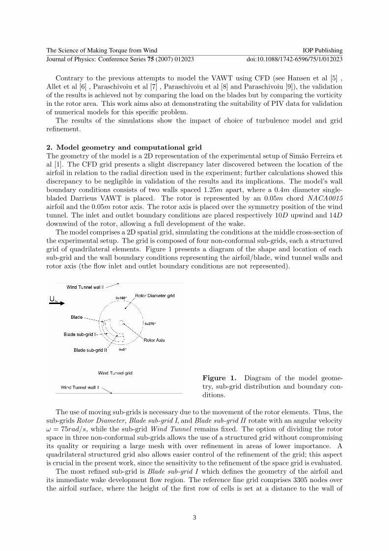
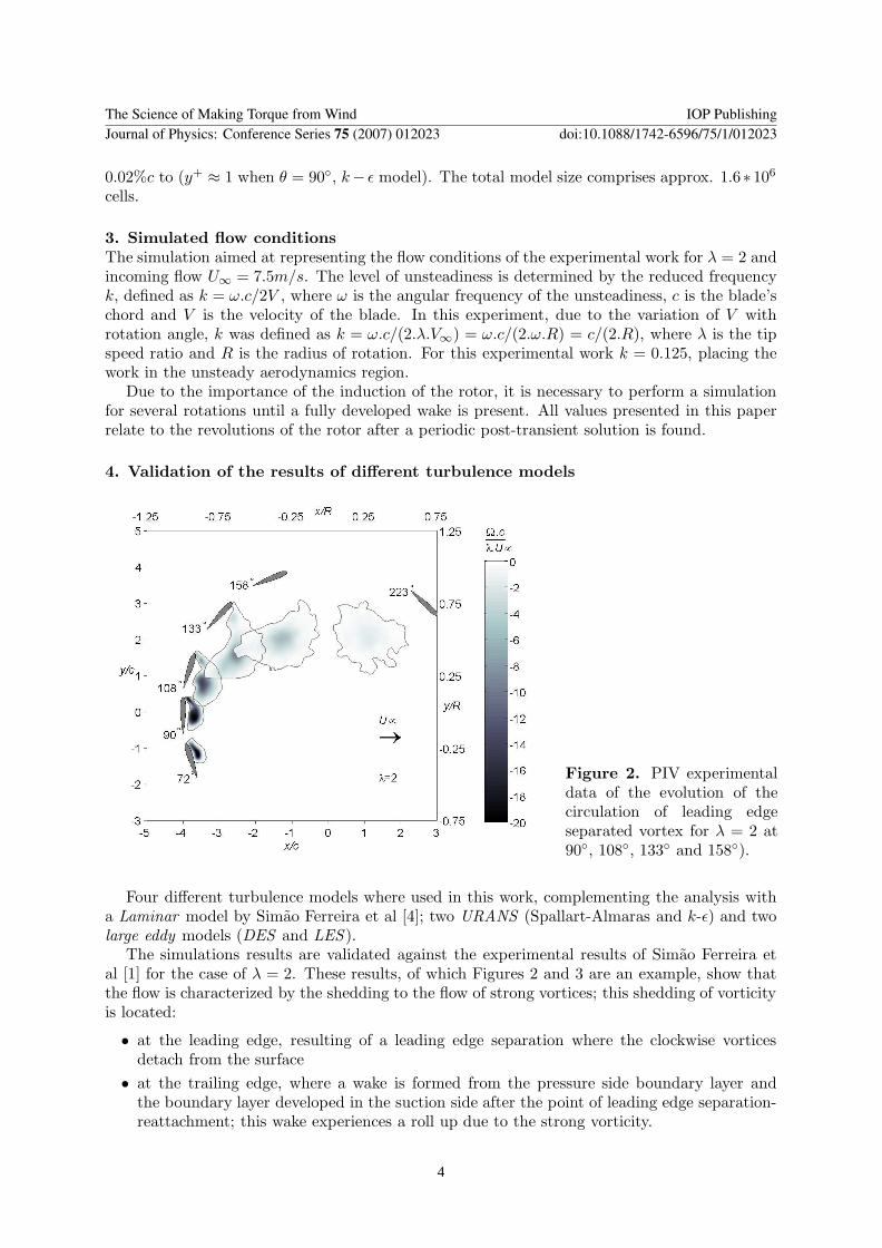
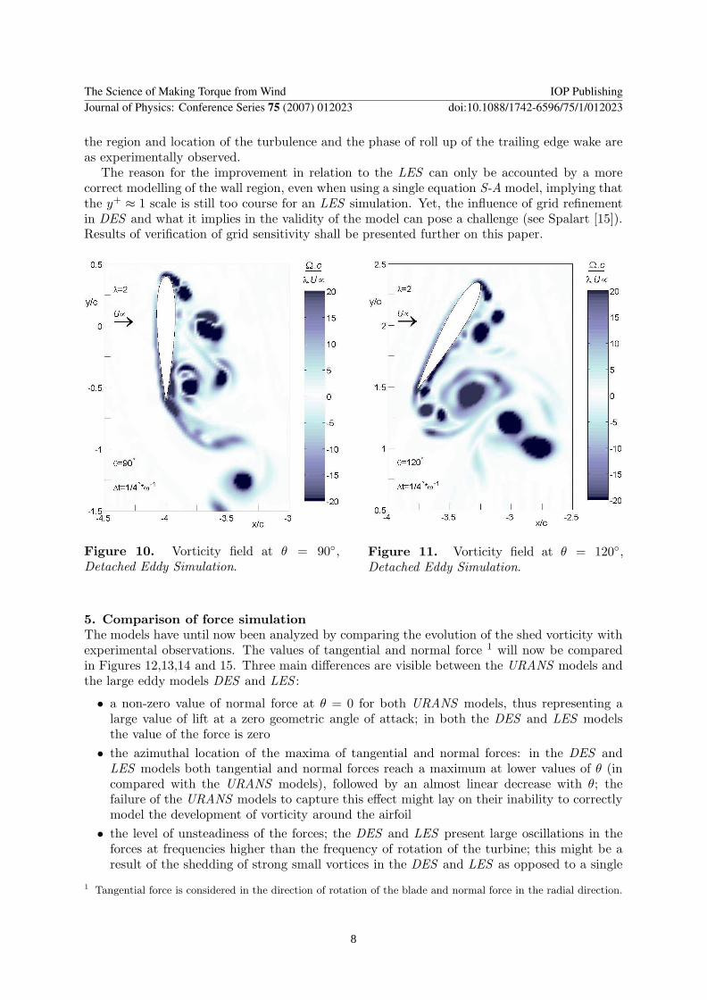
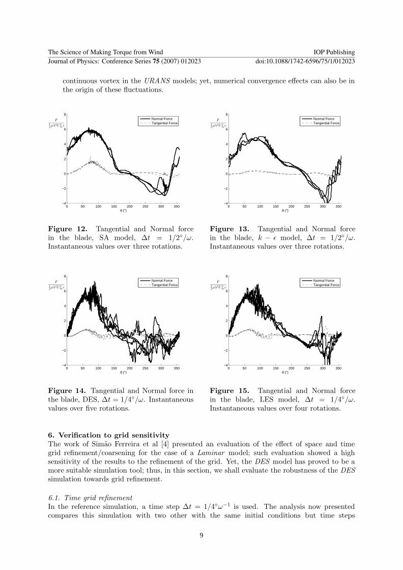