


Languages
Pages
Legal


Seminário de Política Econômica
Tópico 1
Política Monetária: Inflation
Targeting em Mercados Emergentes
(2 de março de 2012, 7h)
Prof. Márcio Garcia
Leituras obrigatórias:
Fraga, A. et al, “Inflation Targeting in Emerging
Market Economies”, in NBER Macroeconomics
Annual 2003.
Mishkin, F., “Can Inflation Targeting Work in
Emerging Market Countries?”, NBER WP # 10646.
FMI, World Economic Outlook, setembro de 2005.
Capítulo IV. Disponível em www.imf.org.
FMI, “Inflation Targeting and the IMF”, 16/03/2006.
Disponível em www.imf.org.
Política Monetária e Fiscal: Inflation
Targeting em Mercados Emergentes
What is inflation targeting? Inflation targeting (IT) has no unanimous definition. Mishkin
[2004] formally defines IT as comprising five components:
the public announcement of medium-term numerical targets for inflation;
an institutional commitment to price stability as the primary goal of monetary policy, to which other goals are subordinated;
an information inclusive strategy in which many variables, and not just monetary aggregates or the exchange rate, are used for deciding the setting of policy instruments;
increased transparency of the monetary policy strategy through communication with the public and the markets about the plans, objectives, and decisions of the monetary authorities; and
increased accountability of the central bank for attaining its inflation objectives.
What is different about IT? According to the World Economic Outlook report (IMF
[2005]), the key distinctions between IT other regimes are the following two. The central bank is mandated, and commits to, a unique
numerical target in the form of a level or a range for annual inflation. A single target for inflation emphasizes the fact that price stabilization is the primary focus of the strategy and the numeric specification provides a guide to what the authorities intend as price stability.
The inflation forecast over some horizon is the de facto intermediate target of policy. For this reason inflation targeting is sometimes referred to as “inflation forecast targeting” (Svensson, 1998). Since inflation is partially predetermined in the short term because of existing price and wage contracts and/or indexation to past inflation, monetary policy can only influence expected future inflation. By altering monetary conditions in response to new information, central banks influence expected inflation and bring it in line over time with the inflation target, which eventually leads actual inflation to the target.
IT and other Monetary Policy Strategies
A synthesis of these two definitions of IT may be found in John Taylor´s remark that the main difference between IT and other monetary policy regimes, e.g. money or exchange rate targeting, was that IT used all the information contained in the macro variables to set the basic interest rate, while other regimes used only part of the information available to determine the interest rate. In a seminal paper (Taylor [1999]), where he analyzed the monetary policy rules implied by the different US monetary policy regimes since 1880, he showed the properties that good monetary policy rules in the US must have, e.g., to respond … to inflation and real output more aggressively than during the 1960s and 1970s or than during the international gold standard—and more like the late 1980s and 1990s. That seems to be the key to successful monetary policy strategies, use of all information to appropriately set interest rates to guide inflation expectations. IT is a way to achieve this.

What are the alternatives to IT?
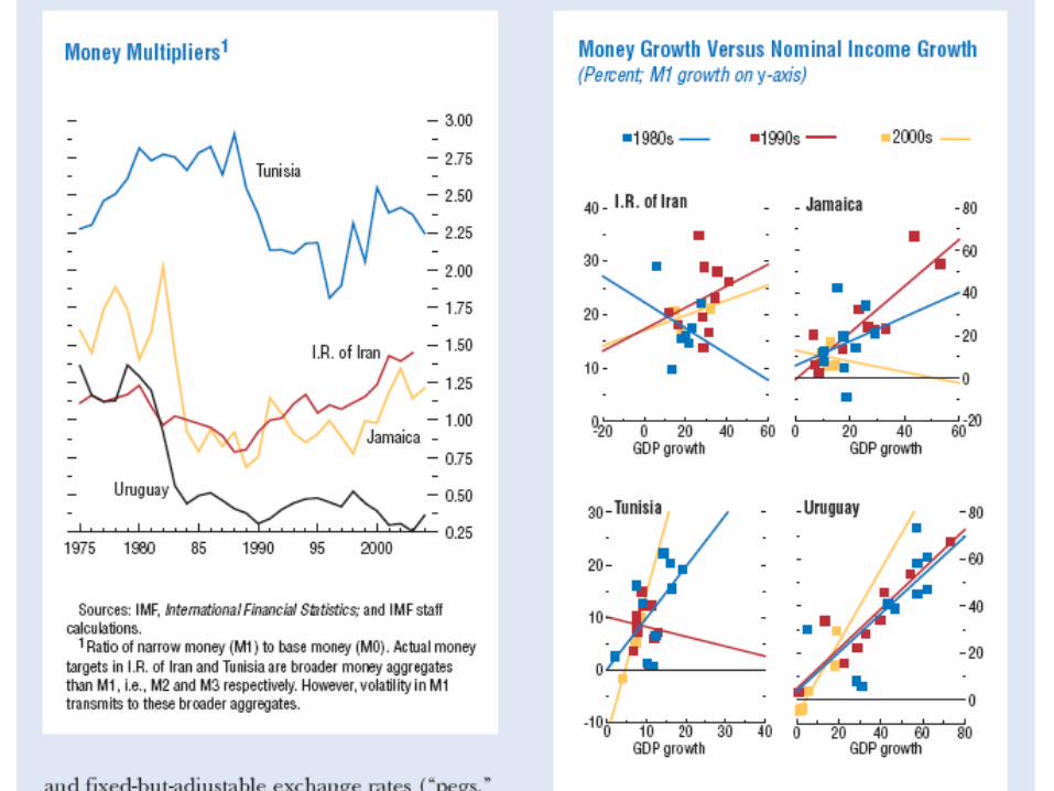
Monetary targeting:
Instability of money demand;
Money multiplier and money velocity vary a lot.
Good for countries where the CB has little credibility and analytical capabilities (money
targeting is very easy to implement and money
data are readily available).
What are the alternatives to IT?
Exchange rate targeting:
Two types:
Fixed exchange rates (currency board, monetary union, and
unilateral dollarization);
Fixed-but-adjustable-exchange rates (crawling pegs,
crawling bands, etc.)
Drawbacks:
Monetary policy is “imported” from a foreign country whose
business cycle may differ;
Possibility of speculative attacks;
Domestic prices bear all the burden of real exchange rate
adjustment.
Why is IT more and more popular?
Because apart from it (or IT) there is only the
Nike™ approach…
How widely used is IT?
In 2005, there were 21 countries that adopted
IT as their monetary policy strategy: eight
industrial countries and 13 emerging markets
(EMs) (IMF [2005]). Table 4.1 of IMF [2005]
lists the inflation targeters, as well as other
relevant information on how IT is
implemented in those countries.
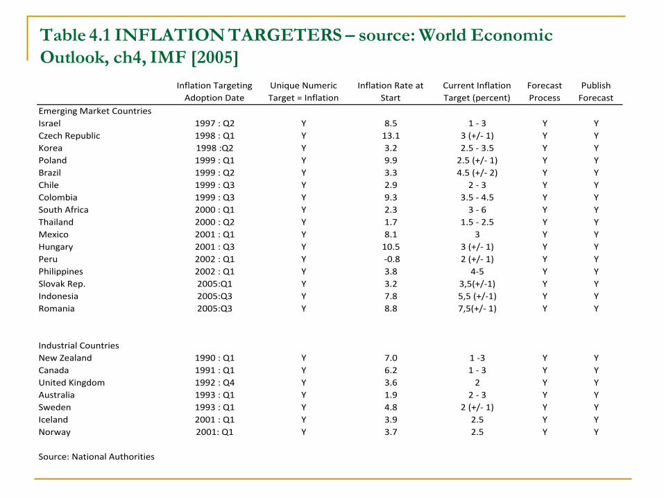
Table 4.1 INFLATION TARGETERS – source: World Economic
Outlook, ch4, IMF [2005]
Inflation Targeting
Adoption Date
Unique Numeric
Target = Inflation
Inflation Rate at
Start
Current Inflation
Target (percent)
Forecast
Process
Publish
Forecast
Emerging Market Countries
Israel 1997 : Q2 Y 8.5 1 - 3 Y Y
Czech Republic 1998 : Q1 Y 13.1 3 (+/- 1) Y Y
Korea 1998 :Q2 Y 3.2 2.5 - 3.5 Y Y
Poland 1999 : Q1 Y 9.9 2.5 (+/- 1) Y Y
Brazil 1999 : Q2 Y 3.3 4.5 (+/- 2) Y Y
Chile 1999 : Q3 Y 2.9 2 - 3 Y Y
Colombia 1999 : Q3 Y 9.3 3.5 - 4.5 Y Y
South Africa 2000 : Q1 Y 2.3 3 - 6 Y Y
Thailand 2000 : Q2 Y 1.7 1.5 - 2.5 Y Y
Mexico 2001 : Q1 Y 8.1 3 Y Y
Hungary 2001 : Q3 Y 10.5 3 (+/- 1) Y Y
Peru 2002 : Q1 Y -0.8 2 (+/- 1) Y Y
Philippines 2002 : Q1 Y 3.8 4-5 Y Y
Slovak Rep. 2005:Q1 Y 3.2 3,5(+/-1) Y Y
Indonesia 2005:Q3 Y 7.8 5,5 (+/-1) Y Y
Romania 2005:Q3 Y 8.8 7,5(+/- 1) Y Y
Industrial Countries
New Zealand 1990 : Q1 Y 7.0 1 -3 Y Y
Canada 1991 : Q1 Y 6.2 1 - 3 Y Y
United Kingdom 1992 : Q4 Y 3.6 2 Y Y
Australia 1993 : Q1 Y 1.9 2 - 3 Y Y
Sweden 1993 : Q1 Y 4.8 2 (+/- 1) Y Y
Iceland 2001 : Q1 Y 3.9 2.5 Y Y
Norway 2001: Q1 Y 3.7 2.5 Y Y
Source: National Authorities

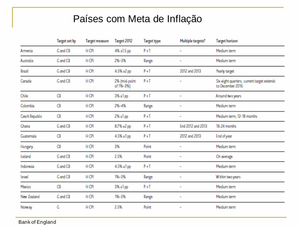
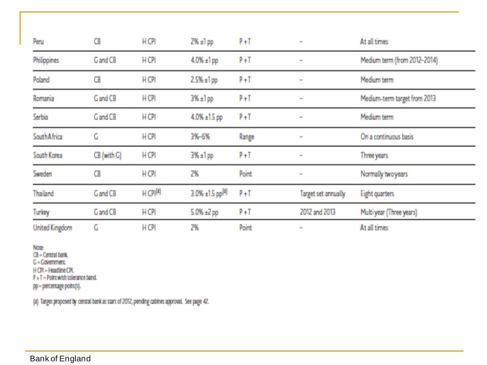
Países com Meta de Inflação
Bank of England
Bank of England
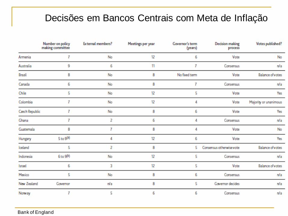
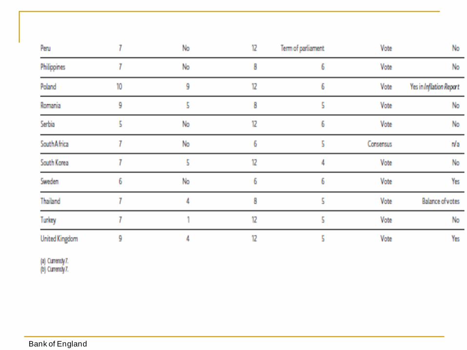
Decisões em Bancos Centrais com Meta de Inflação
Bank of England
Bank of England
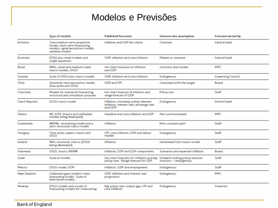
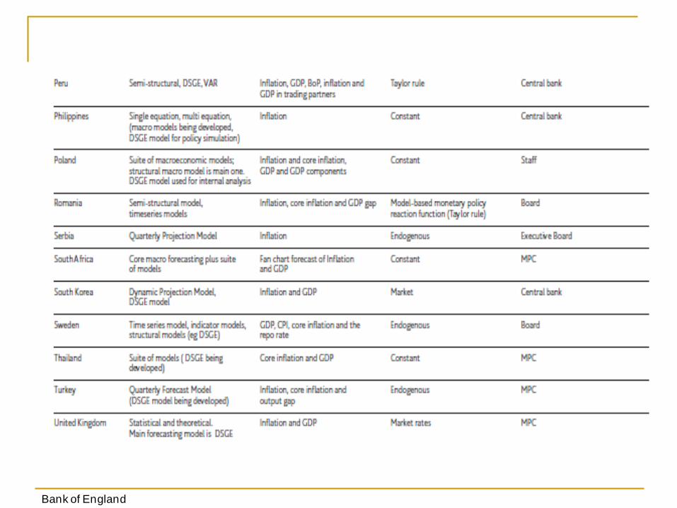
Modelos e Previsões
Bank of England
Bank of England
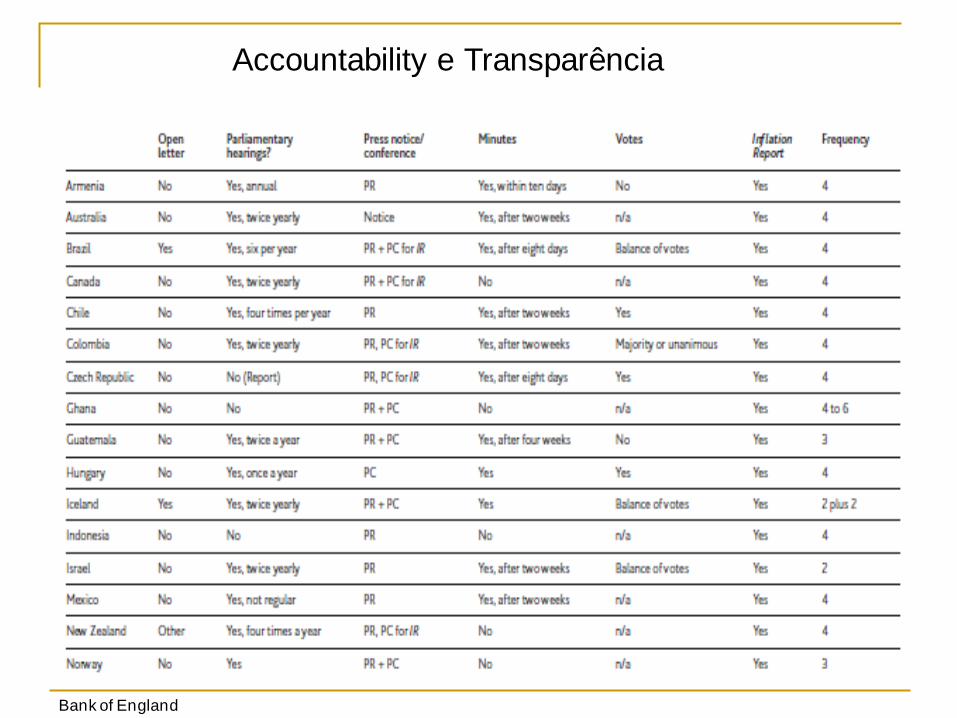
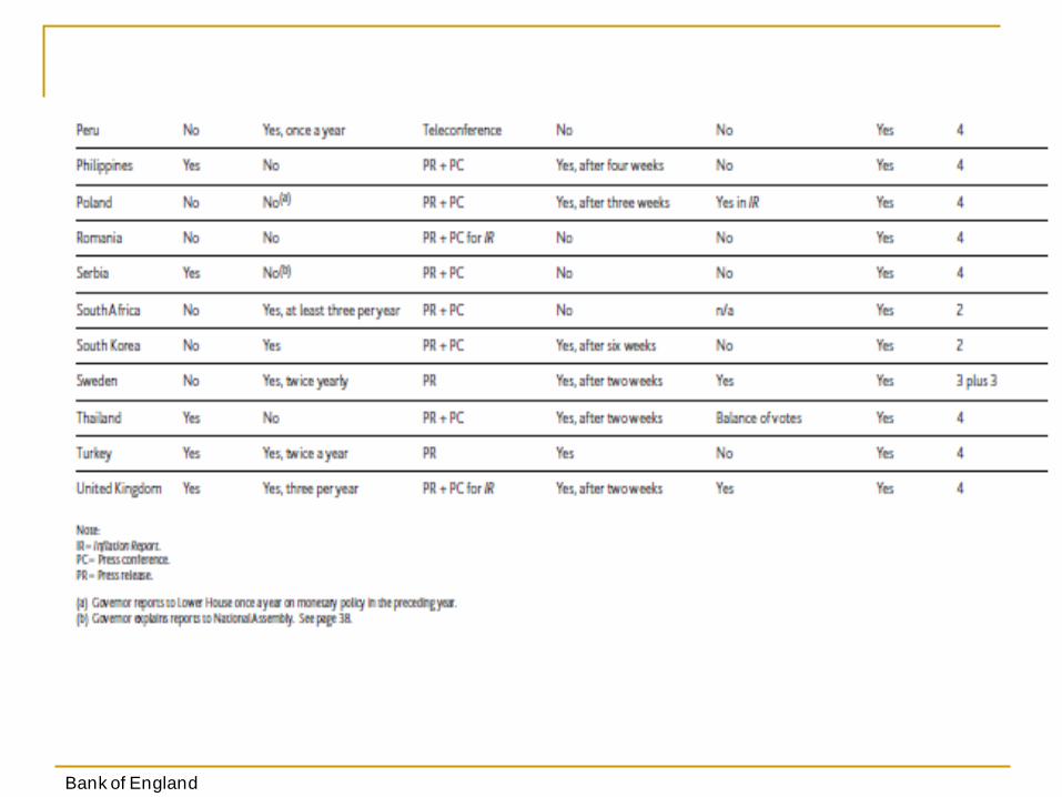
Accountability e Transparência
Bank of England
Bank of England
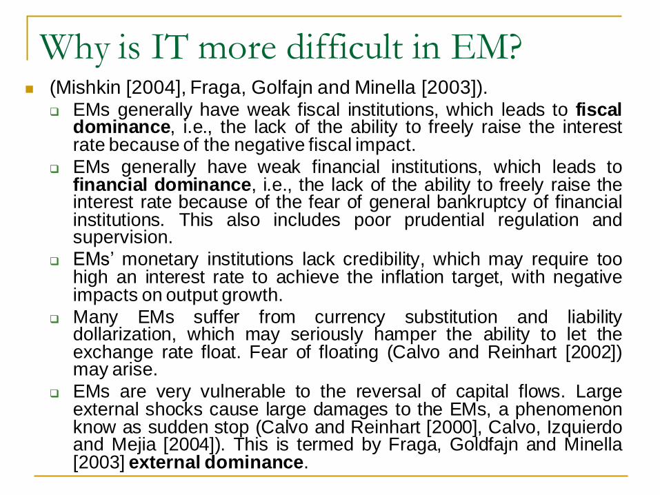
Why is IT more difficult in EM? (Mishkin [2004], Fraga, Golfajn and Minella [2003]).
EMs generally have weak fiscal institutions, which leads to fiscal dominance, i.e., the lack of the ability to freely raise the interest rate because of the negative fiscal impact.
EMs generally have weak financial institutions, which leads to financial dominance, i.e., the lack of the ability to freely raise the interest rate because of the fear of general bankruptcy of financial institutions. This also includes poor prudential regulation and supervision.
EMs’ monetary institutions lack credibility, which may require too high an interest rate to achieve the inflation target, with negative impacts on output growth.
Many EMs suffer from currency substitution and liability dollarization, which may seriously hamper the ability to let the exchange rate float. Fear of floating (Calvo and Reinhart [2002]) may arise.
EMs are very vulnerable to the reversal of capital flows. Large external shocks cause large damages to the EMs, a phenomenon know as sudden stop (Calvo and Reinhart [2000], Calvo, Izquierdo and Mejia [2004]). This is termed by Fraga, Goldfajn and Minella [2003] external dominance.
Is IT suitable for EM?
Even though some of all the factors above
may be true for a given EM, the appraisal of
the experience of the EMs that have opted for
IT seem to run favorably to IT.
Let’s see the empirical evidence…
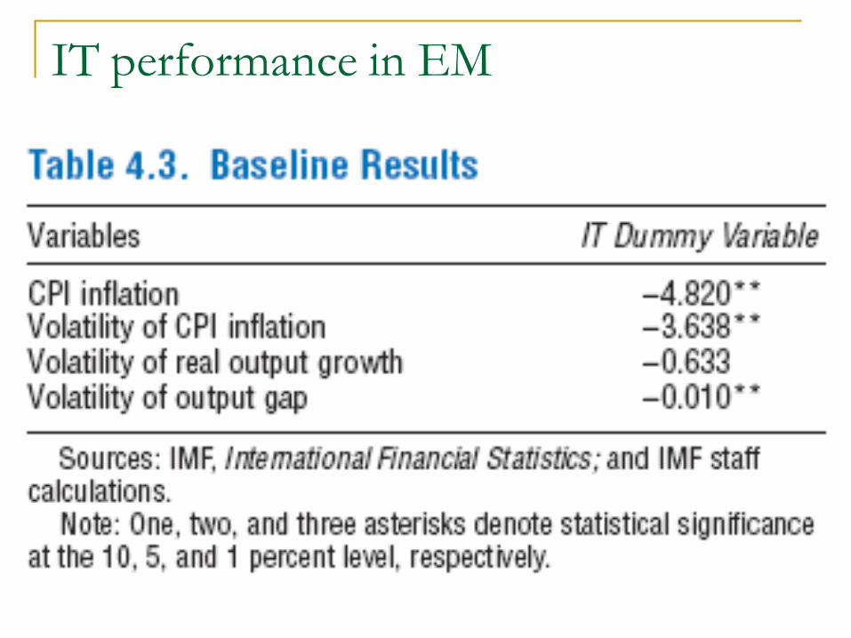
IT performance in EM
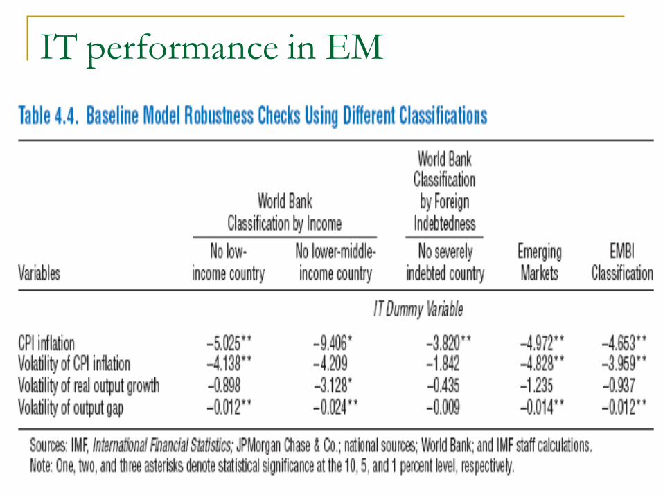
IT performance in EM
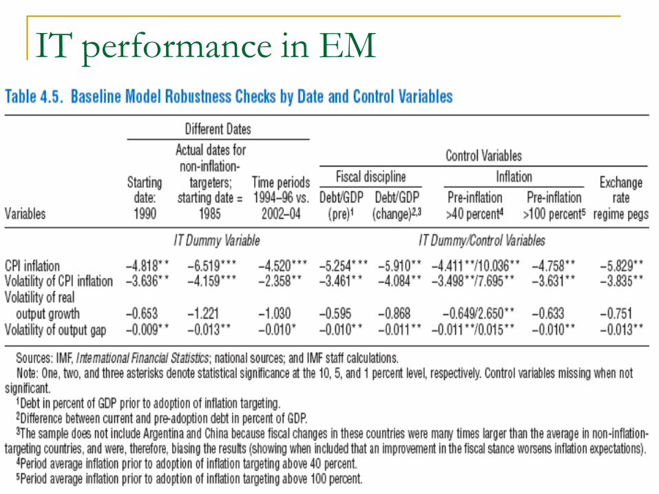
IT performance in EM
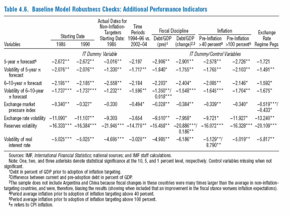
IT performance in EM
IT performance in EM
IT performance in EM
IT performance in EM
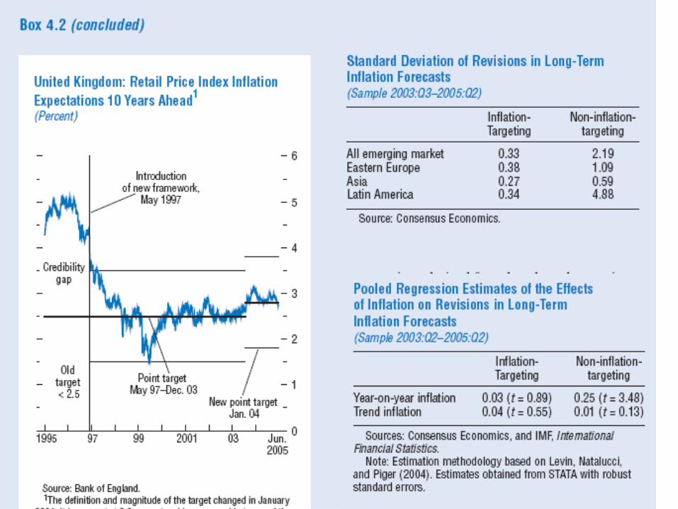
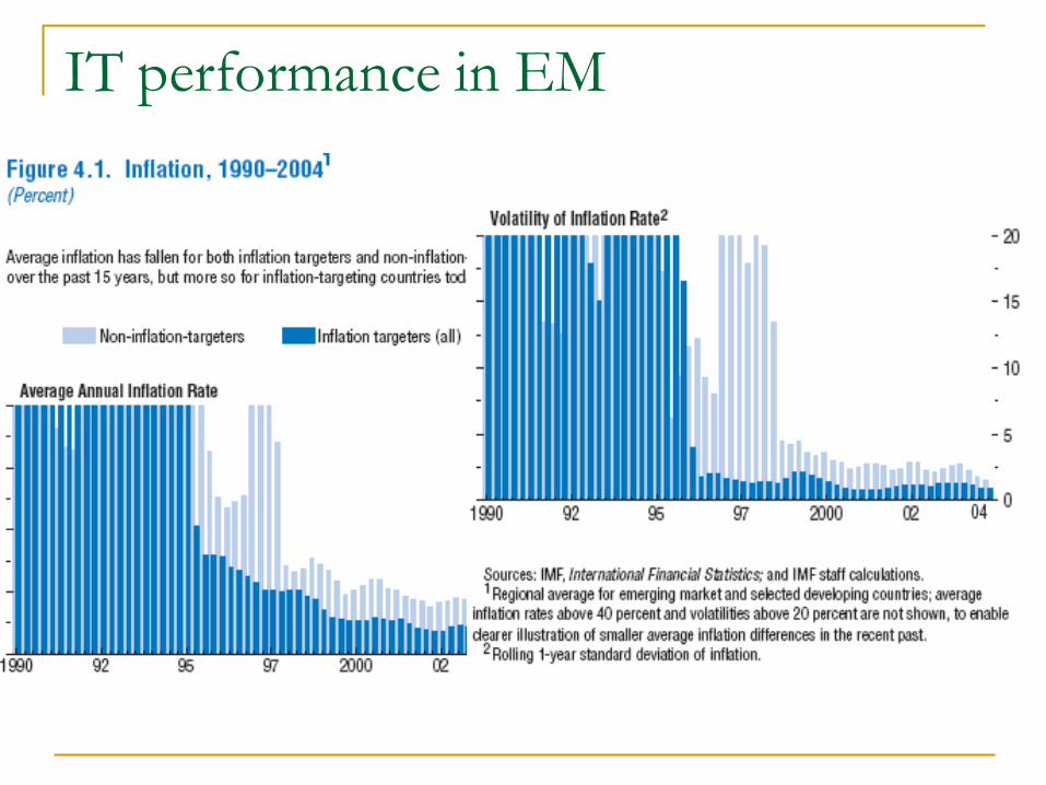
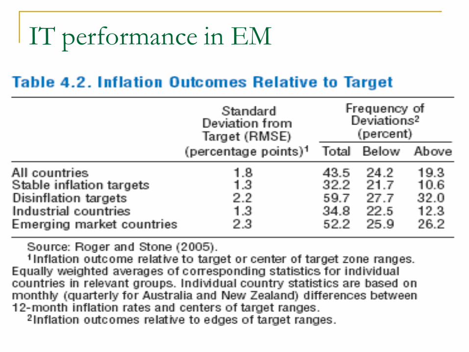
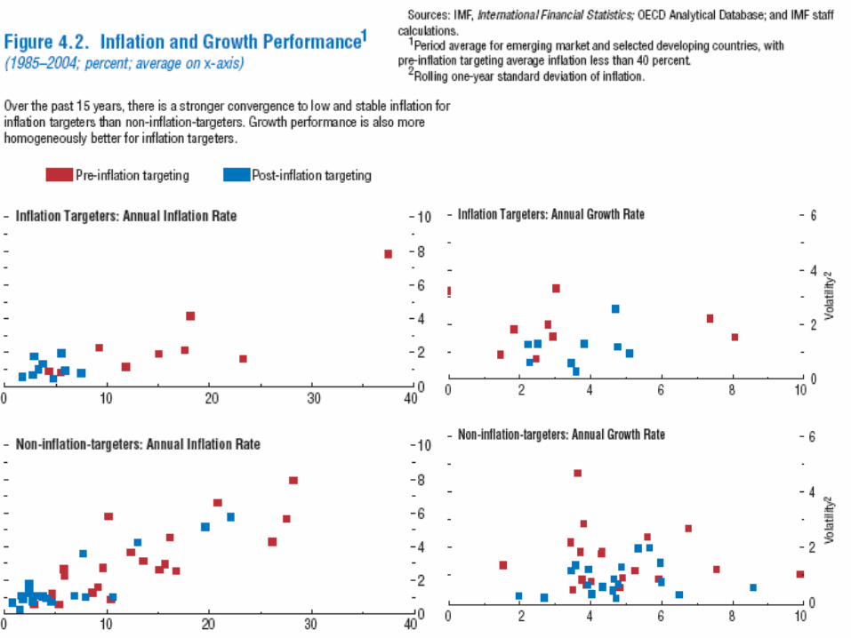
Is IT suitable for EM?
Although the time since the adoption of IT by EMs is short, the IMF report was able to draw a few conclusions regarding the comparative performance of IT and non-IT EMs. … Inflation targeting appears to have been associated with lower inflation, lower inflation expectations, and lower inflation volatility relative to countries that have not adopted it. There have been no visible adverse effects on output, and performance along other dimensions—such as the volatility of interest rates, exchange rates, and international reserves—has also been favorable (IMF [2005]).
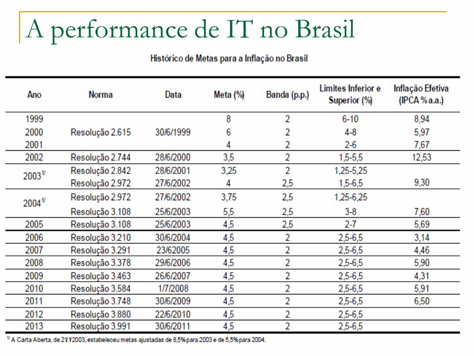
A performance de IT no Brasil
O modelo básico de IT do BCB
O ponto de partida do modelo macroeconômico utilizado pelo BCB para a condução da política monetária no regime de metas de inflação, doravante denominado modelo estrutural, é o trabalho de Bogdanski, Tombini e Werlang (2000)[1]. Trata-se de um modelo com quatro variáveis básicas: a taxa de juros, a taxa de inflação, o hiato do produto e a taxa de câmbio.
[1] Bogdanski, J., A. Tombini e S. Werlang (2000) “Implementing Inflation Targeting in Brazil”, BCB Working Paper Series nº 1.
O modelo básico de IT do BCB:
A curva IS
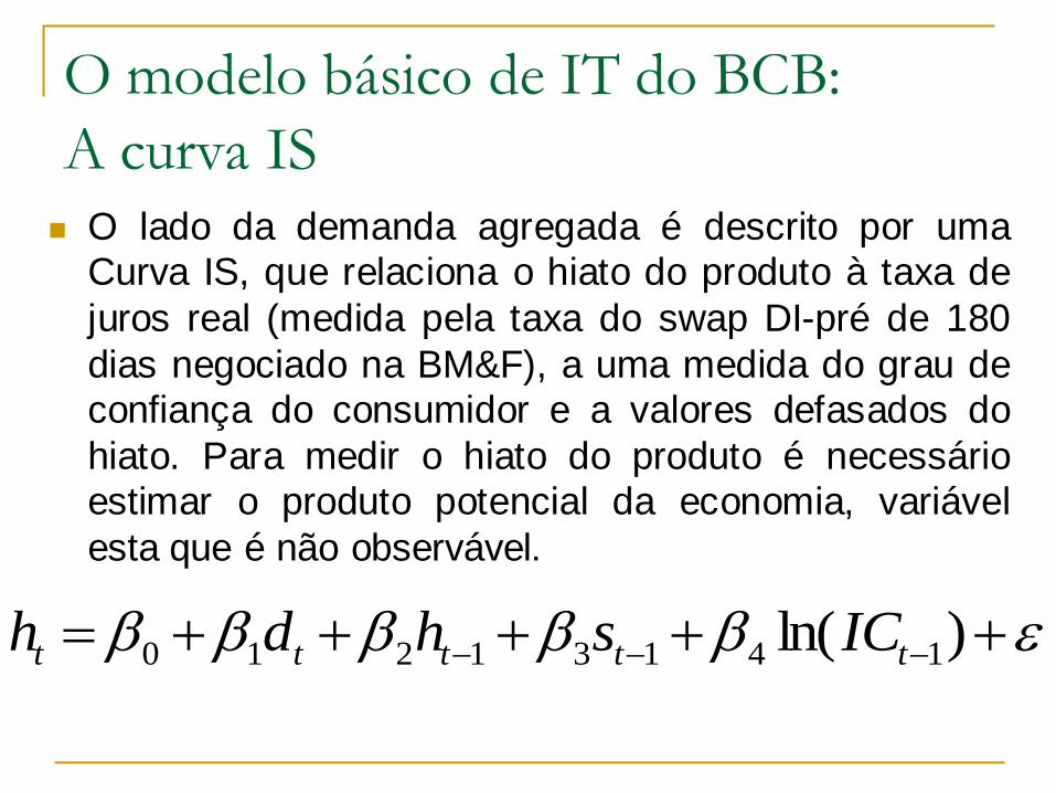
O lado da demanda agregada é descrito por uma Curva IS, que relaciona o hiato do produto à taxa de
juros real (medida pela taxa do swap DI-pré de 180
dias negociado na BM&F), a uma medida do grau de confiança do consumidor e a valores defasados do
hiato. Para medir o hiato do produto é necessário
estimar o produto potencial da economia, variável
esta que é não observável.
)ln( 14131210 ttttt ICshdh

O modelo básico de IT do BCB:
A curva de Phillips O lado da oferta é descrito por uma Curva de Phillips que
relaciona a variação dos preços livres (excluindo os itens “Aluguéis” e “Cursos” do IPCA) a suas variações passadas, ao
hiato do produto e à variação do custo em reais dos bens
importados. Esta última componente incorpora os efeitos da
variação da taxa de câmbio R$/US$ sobre a inflação (pass-
through). Os preços livres são aqueles determinados livremente pelo mercado, e contrastam com os chamados
preços administrados por contrato ou monitorados, cuja
determinação reflete algum tipo de participação do Governo.
tttttttttheeee
25214133221)()(~~~
O modelo básico de IT do BCB:
A taxa de câmbio
De acordo com o BCB, a taxa de câmbio é determinada por uma equação de paridade descoberta da taxa de juros (UIP), ou seja, ela reflete as variações ocorridas nas taxas de juros doméstica e internacional, no prêmio de risco e choques nas expectativas em relação ao seu comportamento futuro. O ajuste econométrico da UIP aos dados é notoriamente ruim.

O modelo básico de IT do BCB:
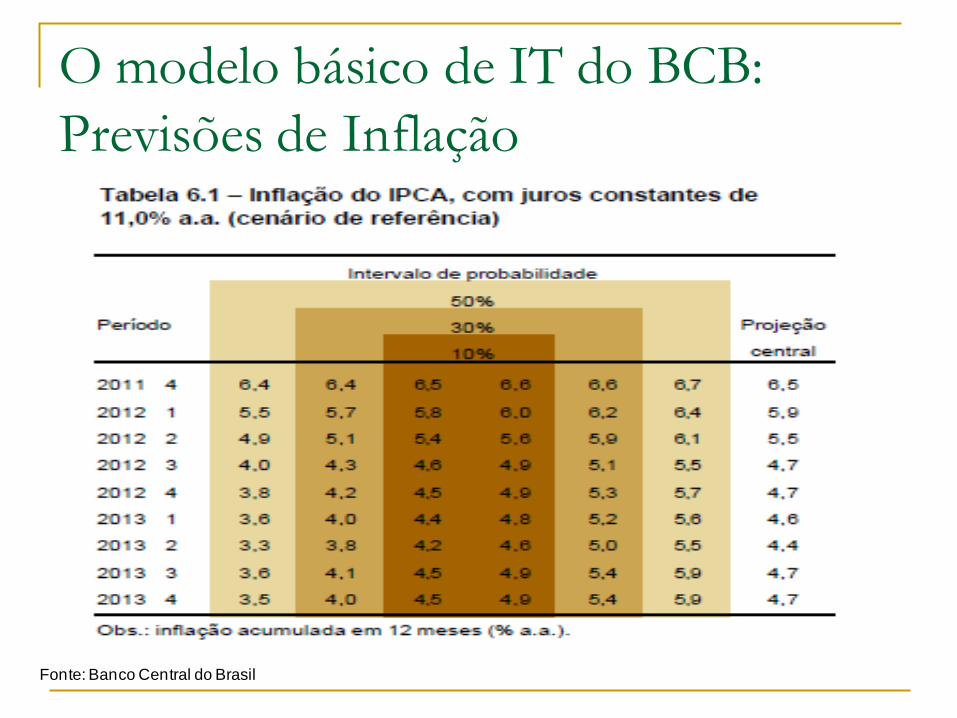
A função de reação do BC
Como o BC é o formulador da função de
reação, ele não divulga uma. O que faz é
divulgar as distribuições de probabilidades
para inflação e crescimento de determinadas
trajetórias das taxas de juros.
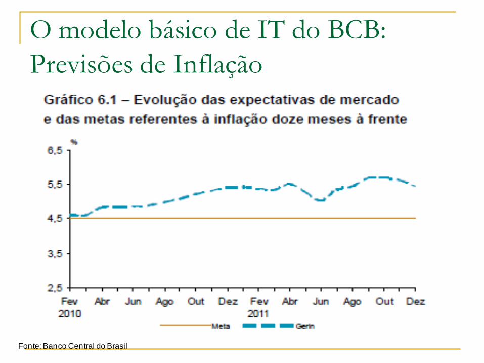
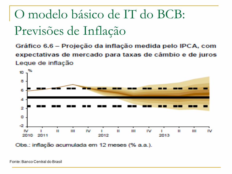
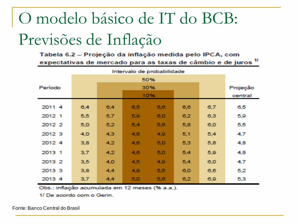
O modelo básico de IT do BCB:
Previsões de Inflação
Fonte: Banco Central do Brasil
O modelo básico de IT do BCB:
Previsões de Inflação
Fonte: Banco Central do Brasil
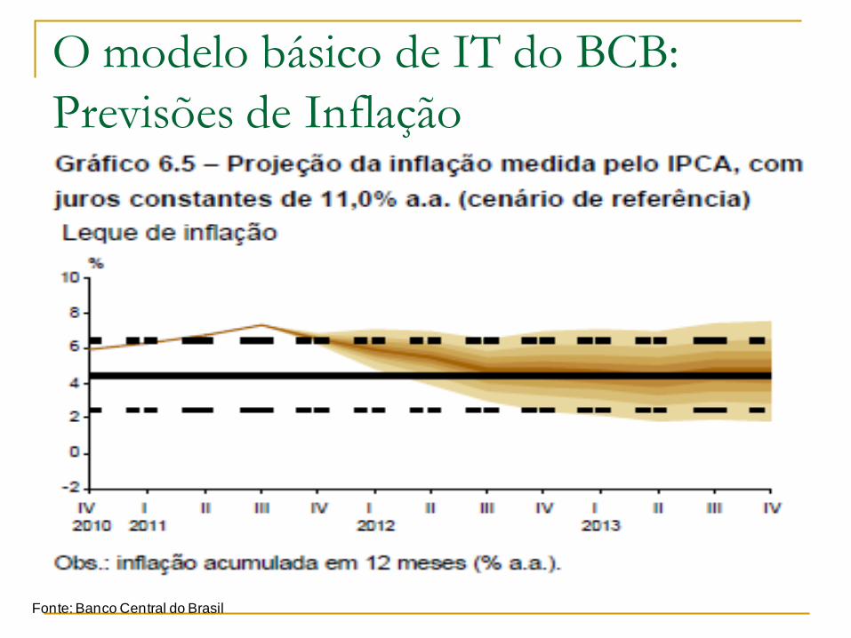
O modelo básico de IT do BCB:
Previsões de Inflação
Fonte: Banco Central do Brasil
O modelo básico de IT do BCB:
Previsões de Inflação
Fonte: Banco Central do Brasil
O modelo básico de IT do BCB:
Previsões de Inflação
Fonte: Banco Central do Brasil
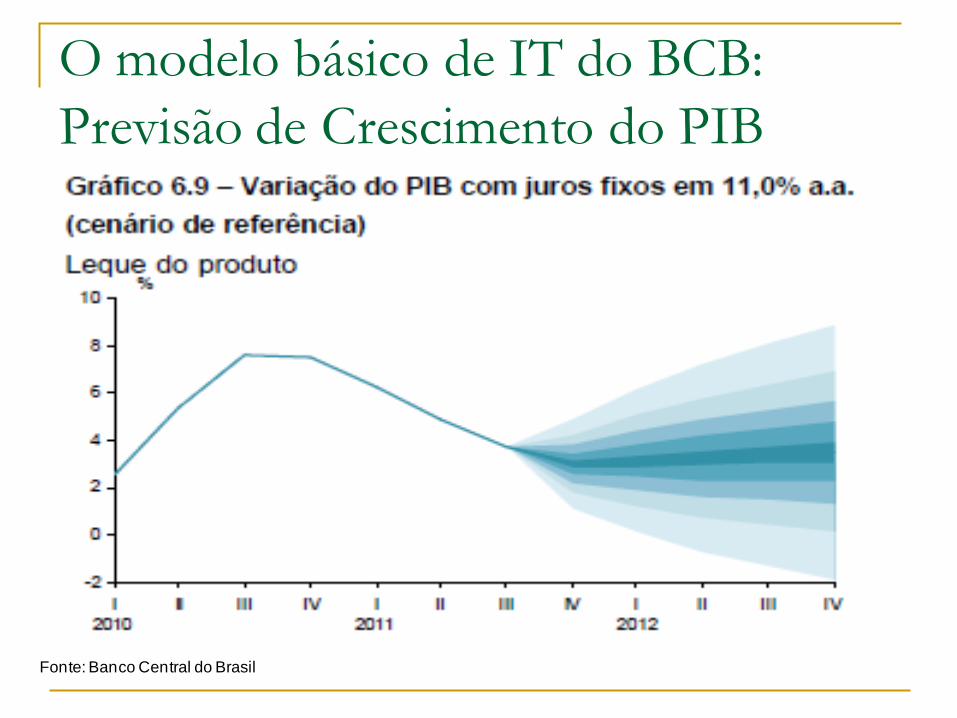
O modelo básico de IT do BCB:
Previsão de Crescimento do PIB
Fonte: Banco Central do Brasil
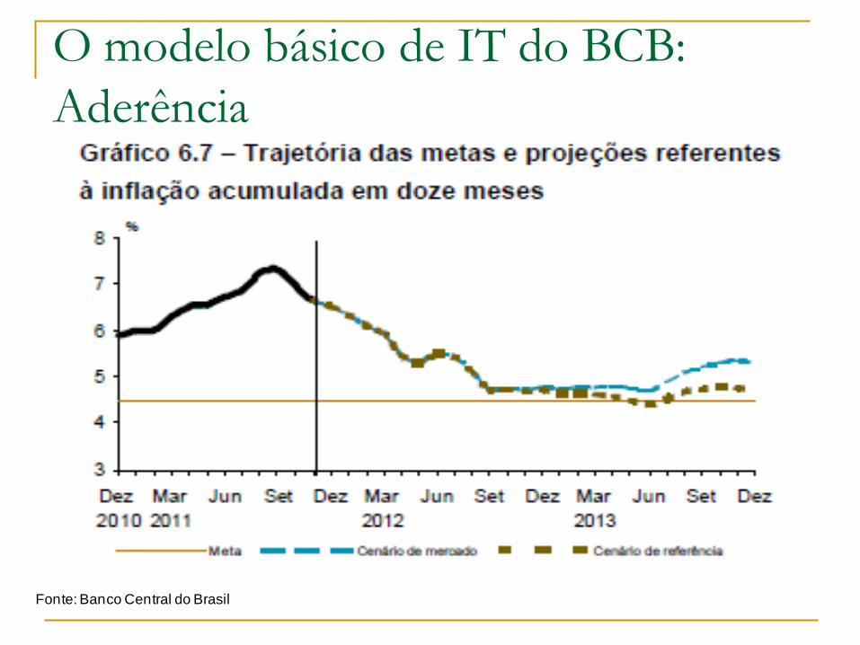
O modelo básico de IT do BCB:
Aderência
Fonte: Banco Central do Brasil


-10%
-9%
-8%
-7%
-6%
-5%
-4%
-3%
-2%
-1%
0%
35%
40%
45%
50%
55%
60%
65%
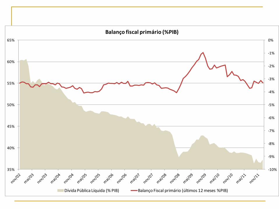
Balanço fiscal primário (%PIB)
Dívida Pública Líquida (% PIB) Balanço Fiscal primário (últimos 12 meses %PIB)
2%
4%
6%
8%
10%
12%
14%
16%
18%
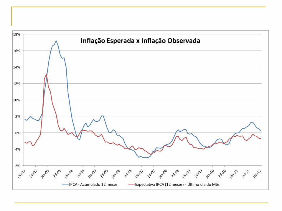
IPCA - Acumulado 12 meses Expectativa IPCA (12 meses) - Último dia do Mês
Inflação Esperada x Inflação Observada
2%
4%
6%
8%
10%
12%
14%
16%
18%
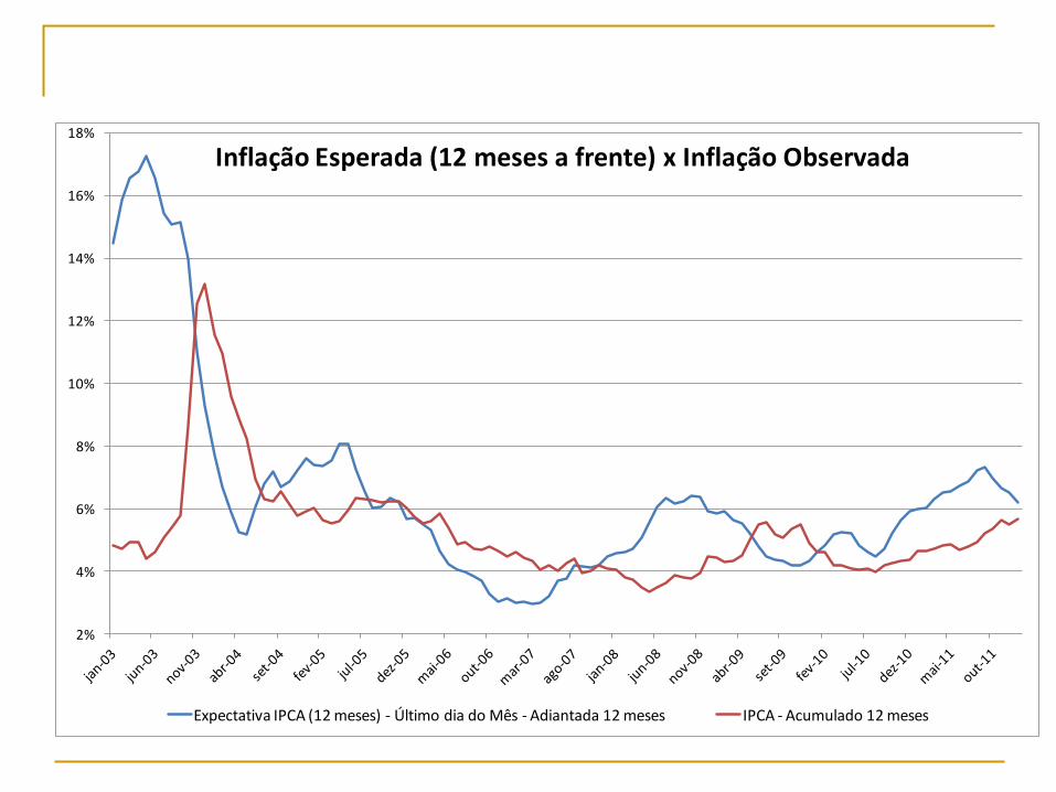
Expectativa IPCA (12 meses) - Último dia do Mês - Adiantada 12 meses IPCA - Acumulado 12 meses
Inflação Esperada (12 meses a frente) x Inflação Observada
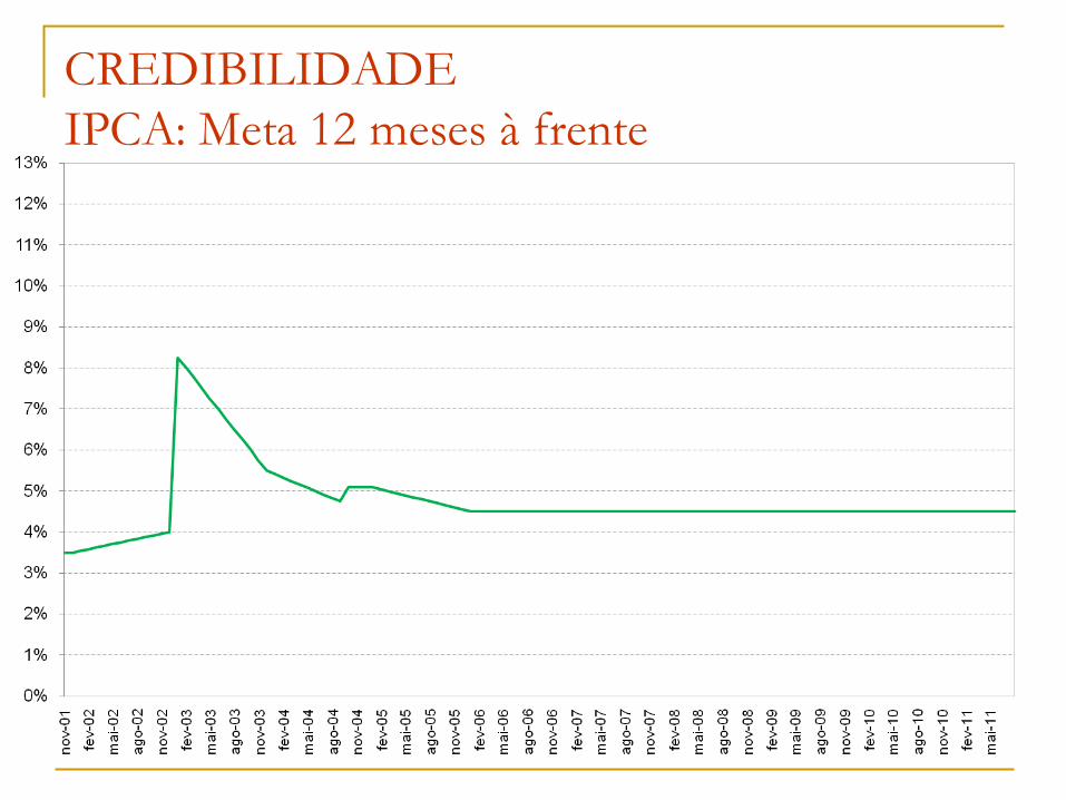
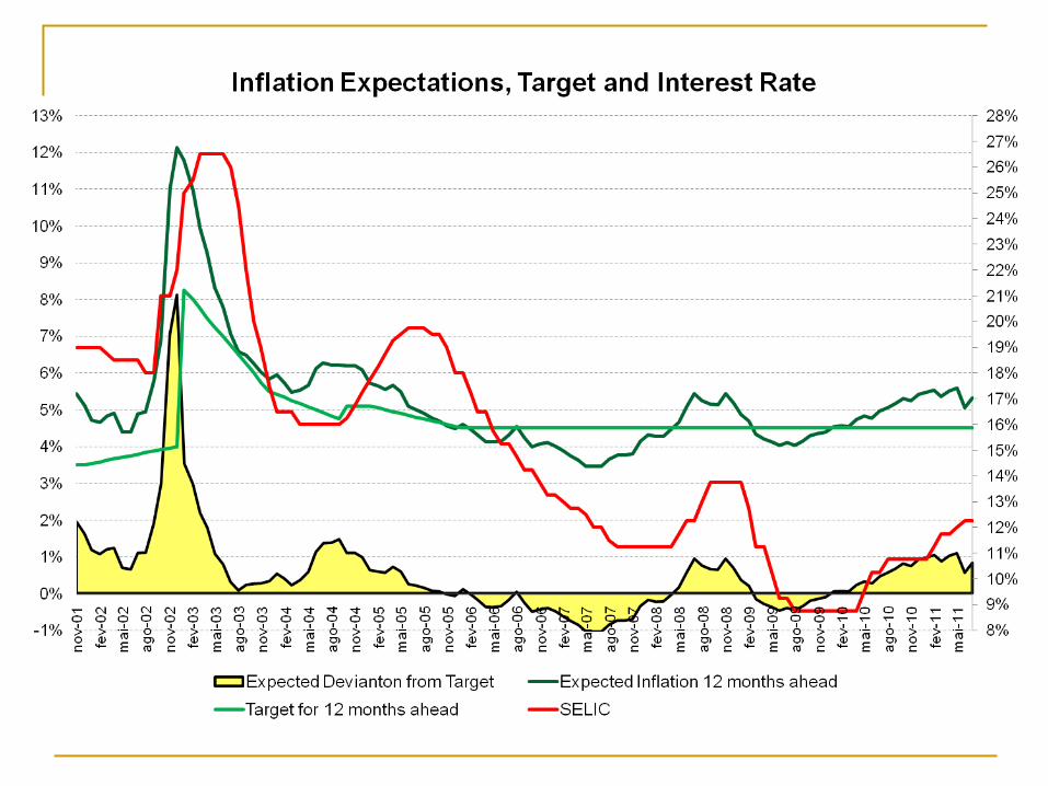
CREDIBILIDADE
IPCA: Meta 12 meses à frente

CREDIBILIDADE
IPCA: Meta e Expectativa 12 meses à frente

CREDIBILIDADE
IPCA: Meta e Expectativa 12 meses à frente
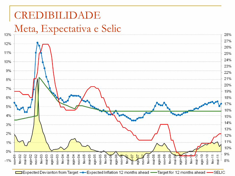
CREDIBILIDADE
Meta, Expectativa e Selic
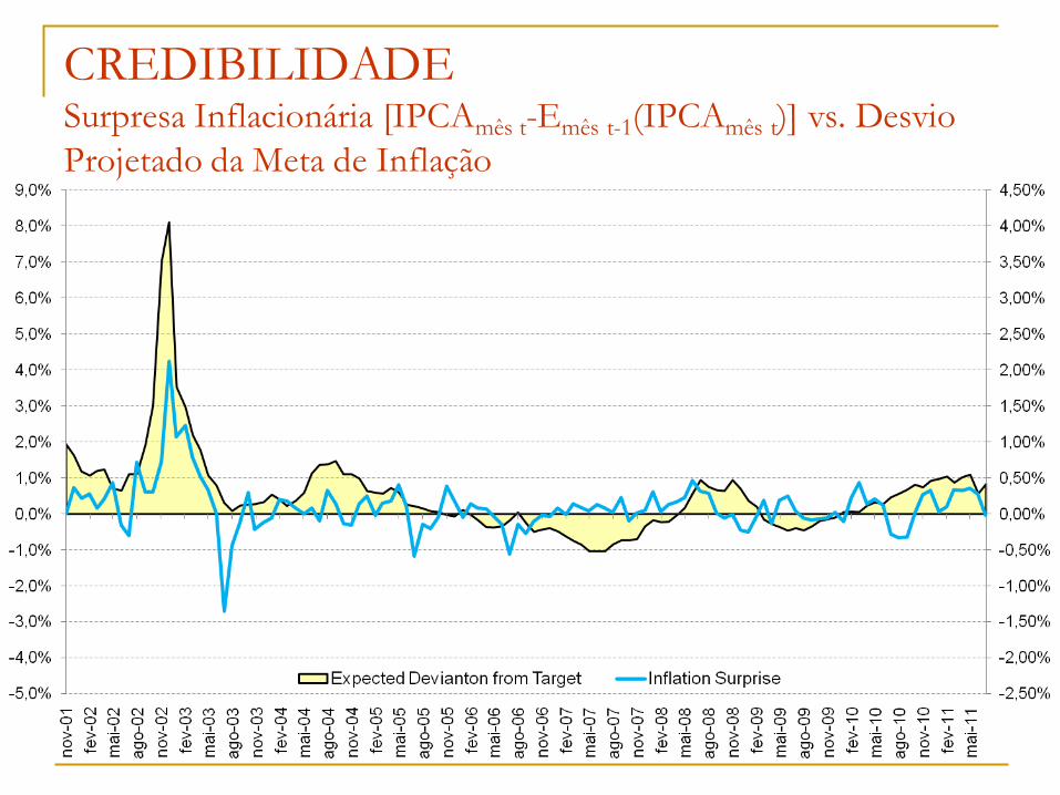
CREDIBILIDADE Surpresa Inflacionária [IPCAmês t-Emês t-1(IPCAmês t)] vs. Desvio
Projetado da Meta de Inflação
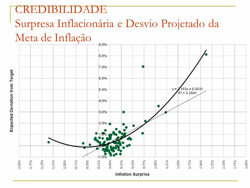
CREDIBILIDADE
Surpresa Inflacionária e Desvio Projetado da
Meta de Inflação
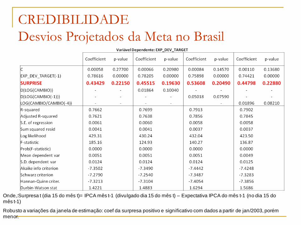
CREDIBILIDADE
Desvios Projetados da Meta no Brasil
Onde,:Surpresa t (dia 15 do mês t)= IPCA mês t-1 (divulgado dia 15 do mês t) – Expectativa IPCA do mês t-1 (no dia 15 do
mês t-1)
Robusto a variações da janela de estimação: coef da surpresa positivo e significativo com dados a partir de jan/2003, porém
menor.

O Efeito da surpresa inflacionária de curto
prazo nas expectativas de médio prazo: uma
comparação internacional
coefficient p-value coefficient p-value coefficient p-value coefficient p-value coefficient p-value coefficient p-value
C 0.000275 0.9924 0.0369133 0.8238 -0.9031188 0.0120 -0.0035178 0.8397 -0.0863169 0.0518 -0.1637156 0.3222
D(INFLA(-1)) 0.0633989 0.3253 0.5213619 0.0223 -0.043515 0.8659 -0.0017427 0.9354 -0.0515741 0.4203 0.1429904 0.4923
D(LOG(CAMBIO(-1))) 2.1412376 0.0271 3.4282796 0.1083 8.8298457 0.0592 -1.2000911 0.1280 2.4876646 0.1579 15.979138 0.0287
D(LOG(COMMODITIES(-1))) -1.6111915 0.0201 -1.7598839 0.6275 -13.069899 0.1615 1.5538316 0.1123 1.073216 0.3291 -3.5902507 0.7343
R-squared 0.2562016 0.1893343 0.1663264 0.1012891 0.1053712 0.0834617
Adjusted R-squared 0.1885835 0.1198486 0.0927669 0.0633154 0.0308188 0.0209705
S.E. of regression 0.1651627 0.7106161 1.462022 0.151313 0.1849389 0.9144702
Sum squared resid 0.9001971 17.674135 72.675279 1.6255883 1.2312866 36.795256
Log likelihood 16.246373 -39.905144 -66.239552 37.265299 12.858856 -61.729079
Durbin-Watson stat 1.4380691 1.1456455 1.3936799 2.0751148 1.832076 1.110601
Mean dependent var -0.0162162 0.02 -0.9473684 -0.004 -0.0665 -0.070125
S.D. dependent var 0.1833538 0.7574542 1.5349508 0.1563434 0.1878563 0.9242122
Akaike info criterion -0.6619661 2.2515459 3.6968185 -0.8870746 -0.4429428 2.7387116
Schwarz criterion -0.4878128 2.4221676 3.869196 -0.7634753 -0.2740548 2.8946451
F-statistic 3.7889528 2.7247971 2.2611154 2.6673491 1.4133845 1.3355744
Prob(F-statistic) 0.0193467 0.0589001 0.0990347 0.0541899 0.254742 0.2749977
Erros-Padrão estimado pelo método Newey-West
MÉXICO
Sample (adjusted):
2001M06 2004M09
Included observations:
40 after adjustments
ISRAEL
Sample (adjusted):
1992M02 1996M01
Included observations:
48 after adjustments
TURKEY UK
Sample (adjusted):
2001M10 2004M11
Included observations:
38 after adjustments
Sample (adjusted):
1997M10 2003M12
Included observations:
75 after adjustments
CHILE
Sample (adjusted):
2001M10 2004M10
Included observations:
37 after adjustments
BRAZIL
Sample (adjusted):
2002M01 2005M03
Included observations:
39 after adjustments
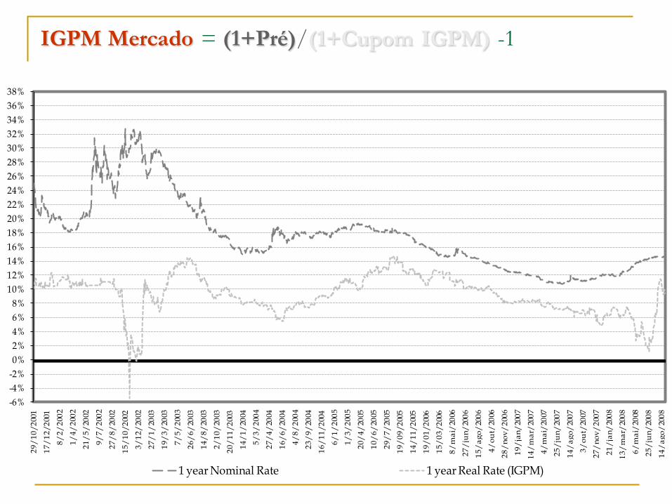
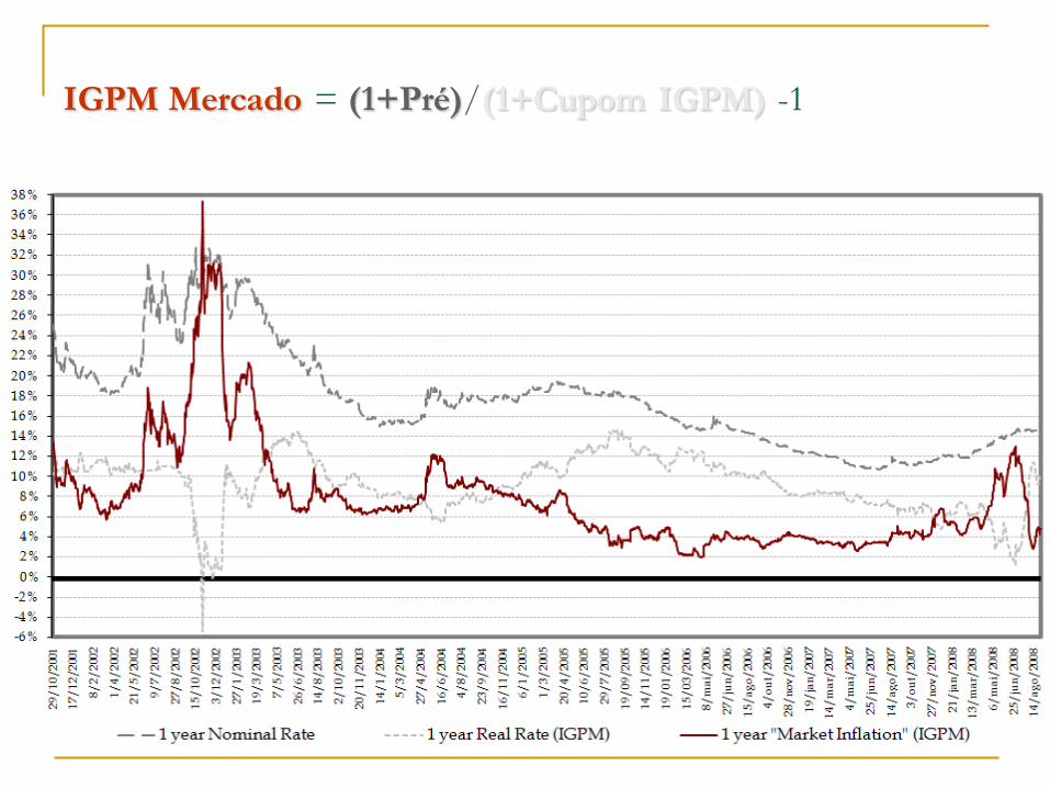
IGPM Mercado = (1+Pré)/(1+Cupom IGPM) -1
-6%
-4%
-2%
0%
2%
4%
6%
8%
10%
12%
14%
16%
18%
20%
22%
24%
26%
28%
30%
32%
34%
36%
38%
29
/1
0/
200
1
17
/1
2/
200
1
8/
2/
200
2
1/
4/
200
2
21
/5
/20
02
9/
7/
200
2
27
/8
/20
02
15
/1
0/
200
2
3/
12
/20
02
27
/1
/20
03
19
/3
/20
03
7/
5/
200
3
26
/6
/20
03
14
/8
/20
03
2/
10
/20
03
20
/1
1/
200
3
14
/1
/20
04
5/
3/
200
4
27
/4
/20
04
16
/6
/20
04
4/
8/
200
4
23
/9
/20
04
16
/1
1/
200
4
6/
1/
200
5
1/
3/
200
5
20
/4
/20
05
10
/6
/20
05
29
/7
/20
05
19
/0
9/
200
5
14
/1
1/
200
5
19
/0
1/
200
6
15
/0
3/
200
6
8/
ma
i/20
06
27
/ju
n/
200
6
15
/a
go
/20
06
4/
ou
t/20
06
28
/n
ov
/2
006
19
/ja
n/
200
7
14
/m
ar/
200
7
4/
ma
i/20
07
25
/ju
n/
200
7
14
/a
go
/20
07
3/
ou
t/20
07
27
/n
ov
/2
007
21
/ja
n/
200
8
13
/m
ar/
200
8
6/
ma
i/20
08
25
/ju
n/
200
8
14
/a
go
/20
08
1 year Nominal Rate 1 year Real Rate (IGPM)
IGPM Mercado = (1+Pré)/(1+Cupom IGPM) -1
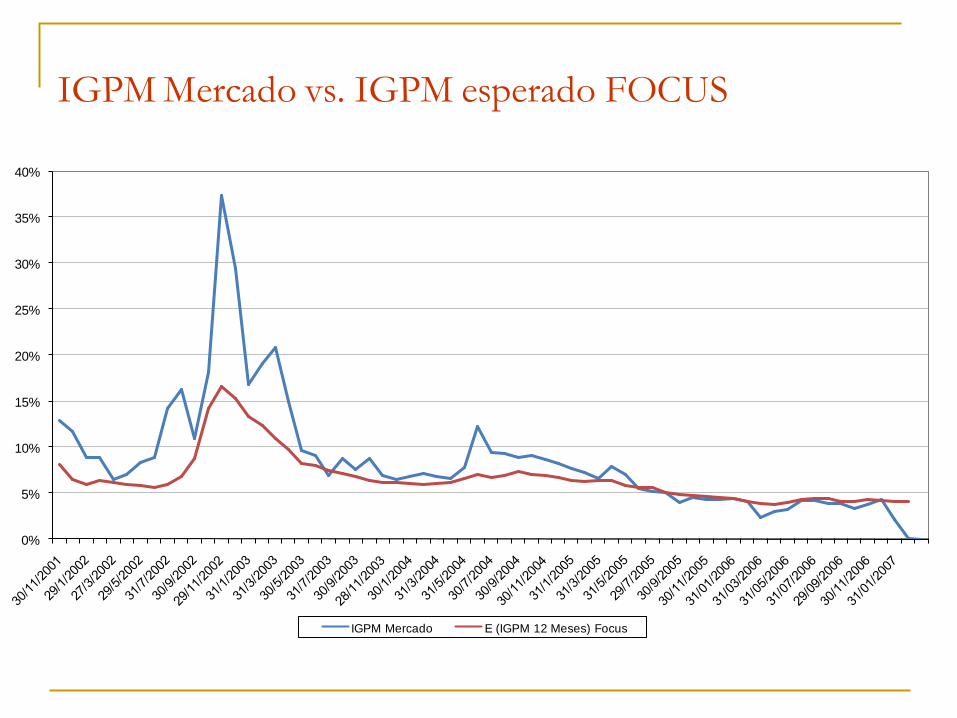
IGPM Mercado vs. IGPM esperado FOCUS
0%
5%
10%
15%
20%
25%
30%
35%
40%
IGPM Mercado E (IGPM 12 Meses) Focus
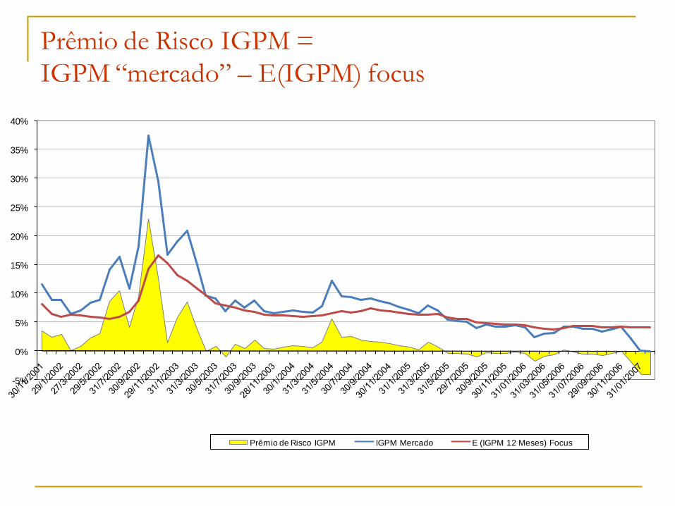
Prêmio de Risco IGPM =
IGPM “mercado” – E(IGPM) focus
-5%
0%
5%
10%
15%
20%
25%
30%
35%
40%
Prêmio de Risco IGPM IGPM Mercado E (IGPM 12 Meses) Focus
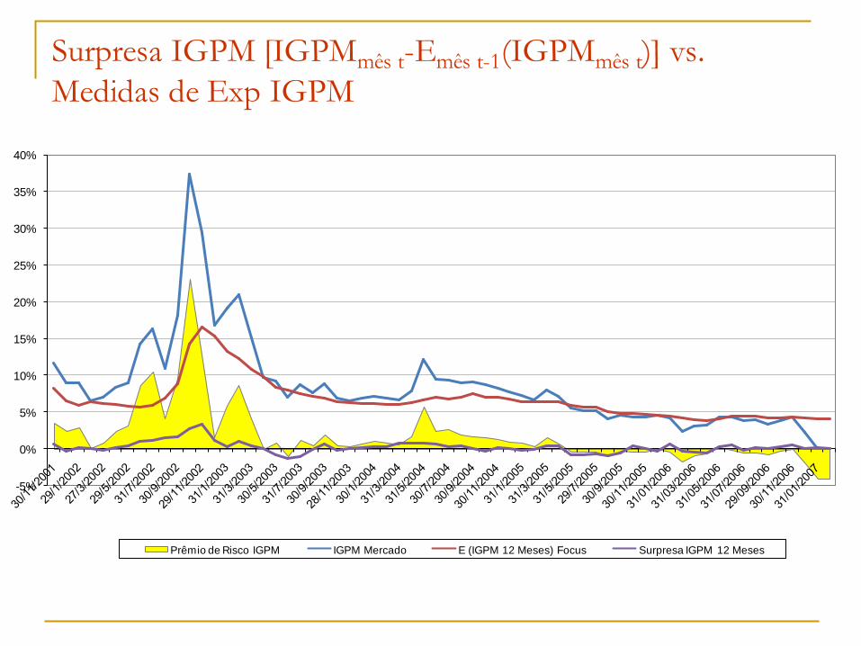
Surpresa IGPM [IGPMmês t-Emês t-1(IGPMmês t)] vs.
Medidas de Exp IGPM
-5%
0%
5%
10%
15%
20%
25%
30%
35%
40%
Prêmio de Risco IGPM IGPM Mercado E (IGPM 12 Meses) Focus Surpresa IGPM 12 Meses
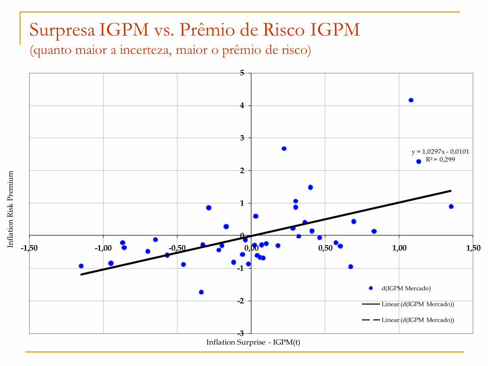
Surpresa IGPM vs. Prêmio de Risco IGPM (quanto maior a incerteza, maior o prêmio de risco)
y = 1,0297x - 0,0101R² = 0,299
-3
-2
-1
0
1
2
3
4
5
-1,50 -1,00 -0,50 0,00 0,50 1,00 1,50Infl
ati
on
Ris
k P
rem
ium
Inflation Surprise - IGPM(t)
d(IGPM Mercado)
Linear (d(IGPM Mercado))
Linear (d(IGPM Mercado))
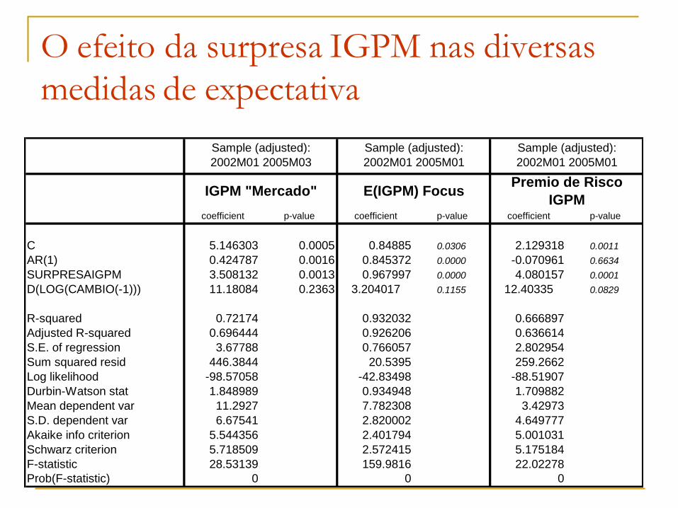
O efeito da surpresa IGPM nas diversas
medidas de expectativa
coefficient p-value coefficient p-value coefficient p-value
C 5.146303 0.0005 0.84885 0.0306 2.129318 0.0011
AR(1) 0.424787 0.0016 0.845372 0.0000 -0.070961 0.6634
SURPRESAIGPM 3.508132 0.0013 0.967997 0.0000 4.080157 0.0001
D(LOG(CAMBIO(-1))) 11.18084 0.2363 3.204017 0.1155 12.40335 0.0829
R-squared 0.72174 0.932032 0.666897
Adjusted R-squared 0.696444 0.926206 0.636614
S.E. of regression 3.67788 0.766057 2.802954
Sum squared resid 446.3844 20.5395 259.2662
Log likelihood -98.57058 -42.83498 -88.51907
Durbin-Watson stat 1.848989 0.934948 1.709882
Mean dependent var 11.2927 7.782308 3.42973
S.D. dependent var 6.67541 2.820002 4.649777
Akaike info criterion 5.544356 2.401794 5.001031
Schwarz criterion 5.718509 2.572415 5.175184
F-statistic 28.53139 159.9816 22.02278
Prob(F-statistic) 0 0 0
Sample (adjusted):
2002M01 2005M01
Premio de Risco
IGPM
Sample (adjusted):
2002M01 2005M03
E(IGPM) Focus
Sample (adjusted):
2002M01 2005M01
IGPM "Mercado"
CREDIBILIDADE
Surpresas de curto prazo da inflação no Brasil (IPCA e IGPM) levam a
uma grande correção nas expectativas de médio prazo, mesmo controlando para choques do câmbio.
Este efeito não foi encontrado nos outros países analisados.
Duas principais razões (e/ou):
Falta de credibilidade da autoridade monetária.
Excessiva indexação da economia.
O fato de o prêmio de risco inflacionário ser extremamente correlacionado com a medida de surpresa inflacionária implica que, pelo menos em parte, o problema se deve à falta de credibilidade da autoridade monetária.
Can IT deliver sustained growth in
Brazil? The five problematic points for IT in EM were:
1) Fiscal dominance;
2) Financial dominance;
3) Low credibility;
4) Liability dollarization and currency substitution;
5) External dominance.
Brazil suffers from 1, although the CB has behaved as if it did not. How long may this behavior continue without compromising debt sustainability? 3 used to be a problem, but it is solved as long as the “right” people are at the helm of the CB (CB independence would greatly help). 5 is not currently a problem given the massive, quickly and costly dedollarization undertaken. 2 and 4 were never a problem for Brazil.

Given the strong performance of the export sector, external dominance seem to be a much smaller risk in
the medium run.
By fiercily pursuing the inflation target, the BCB has achieved as much credibility as possible in the current
institutional arrangement. Granting instrument (not
goal) independence to the BCB would be a free lunch.
Fiscal sustainability in the medium and long runs, despite the current high primary surplus, remain the
largest risk.
Can IT deliver sustained growth in
Brazil?
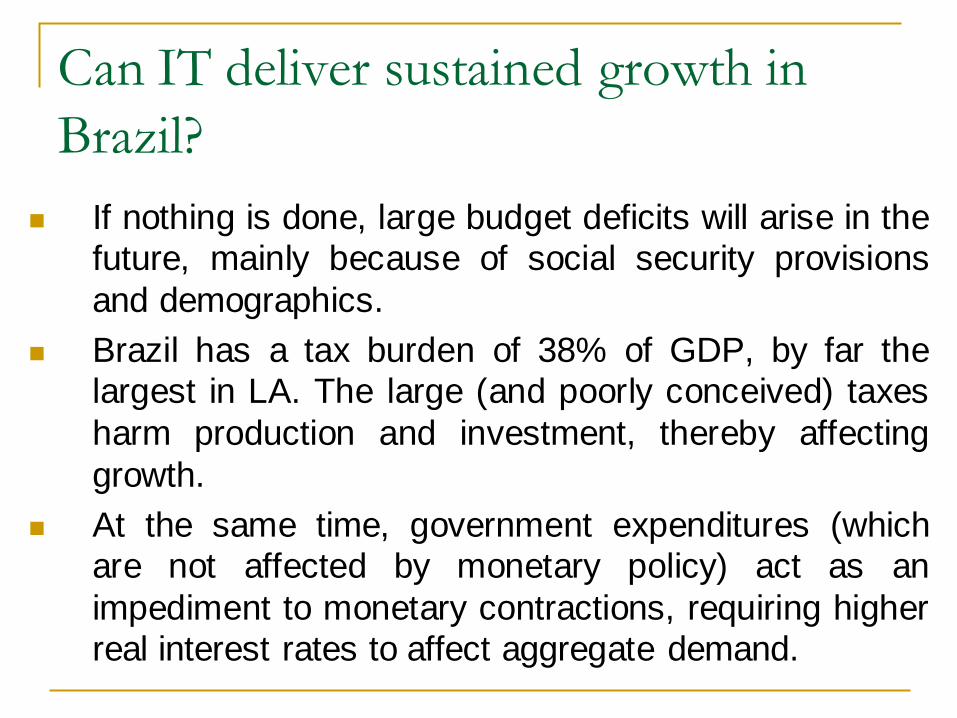
If nothing is done, large budget deficits will arise in the future, mainly because of social security provisions
and demographics.
Brazil has a tax burden of 38% of GDP, by far the largest in LA. The large (and poorly conceived) taxes
harm production and investment, thereby affecting
growth.
At the same time, government expenditures (which
are not affected by monetary policy) act as an
impediment to monetary contractions, requiring higher real interest rates to affect aggregate demand.
Can IT deliver sustained growth in
Brazil?

Lessons for other Emerging Markets
IT can work in EM despite their fragilities;
The IT framework makes monetary policy more
transparent and, therefore, credible;
IT acts as better tool to align inflation expectations;
IT helps to achieve better economic policy in general,
by making clear who the true culprits of low growth and
unemployment are. In that sense, it helps to build the
institutional framework conducive to sustained growth,
as the fiscal responsibilty law.
IT must include escape clauses in face of large external shocks, as the Brazilian provision to deal
with administered prices shocks and exchange rate
shocks.
Top Related