Roofline: An Insightful Visual Performance Model forFloating-Point Programs and Multicore Architectures

Samuel Webb WilliamsAndrew WatermanDavid A. Patterson

Electrical Engineering and Computer SciencesUniversity of California at Berkeley

Technical Report No. UCB/EECS-2008-134

http://www.eecs.berkeley.edu/Pubs/TechRpts/2008/EECS-2008-134.html

October 17, 2008

Copyright 2008, by the author(s).All rights reserved.

Permission to make digital or hard copies of all or part of this work forpersonal or classroom use is granted without fee provided that copies arenot made or distributed for profit or commercial advantage and that copiesbear this notice and the full citation on the first page. To copy otherwise, torepublish, to post on servers or to redistribute to lists, requires prior specificpermission.

*Submitted to Communications of the ACM April 2008. Revised August and October 2008.

Roofline: An Insightful Visual Performance Model for Floating-Point Programs and Multicore Architectures*

Samuel Williams, Andrew Waterman, and David Patterson Parallel Computing Laboratory, 565 Soda Hall, U.C. Berkeley, Berkeley, CA 94720-1776, 510-642-6587

samw, waterman, pattrsn@eecs.berkeley.eduABSTRACT We propose an easy-to-understand, visual performance model that offers insights to programmers and architects on improving parallel software and hardware for floating point computations.

1. INTRODUCTION Conventional wisdom in computer architecture led to homogeneous designs. Nearly every desktop and server computer uses caches, pipelining, superscalar instruction issue, and out-of-order execution. Although the instruction sets varied, the microprocessors were all from the same school of design.

The switch to multicore means that microprocessors will become more diverse, since there is no conventional wisdom yet for them. For example, some offer many simple processors versus fewer complex processors, some depend on multithreading, and some even replace caches with explicitly addressed local stores. Manufacturers will likely offer multiple products with differing number of cores to cover multiple price-performance points, since the cores per chip will likely double every two years [4].

While diversity may be understandable in this time of uncertainty, it exacerbates the already difficult job of programmers, compiler writers, and even architects. Hence, an easy-to-understand model that offers performance guidelines could be especially valuable.

A model need not be perfect, just insightful. For example, the 3Cs model for caches is an analogy [19]. It is not a perfect model, since it ignores potentially important factors like block size, block allocation policy, and block replacement policy. Moreover, it has quirks. For example, a miss can be labeled capacity in one design and conflict in another cache of the same size. Yet, the 3Cs model has been popular for nearly 20 years because it offers insights into the behavior of programs, helping programmers, compiler writers, and architects improve their respective designs.

This paper proposes such a model and demonstrates it on four diverse multicore computers using four key floating-point kernels.

2. PERFORMANCE MODELS Stochastic analytical models [14][28] and statistical performance models [7][27] can predict program performance on multiprocessors accurately. However, they rarely provide insights into how to improve performance of programs, compilers, or computers [1] or they can be hard to use by non-experts [27].

An alternative, simpler approach is bound and bottleneck analysis. Instead of trying to predict performance, it provides [20]

“valuable insight into the primary factors affecting the performance of computer systems. In particular, the critical influence of the system bottleneck is highlighted and quantified.”

The best-known example is surely Amdahl’s Law [3], which states simply that the performance gain of a parallel computer is

limited by the serial portion of a parallel program. It has been recently applied to heterogeneous multicore computers [4][18].

3. THE ROOFLINE MODEL We believe that for the recent past and foreseeable future, off-chip memory bandwidth will often be the constraining resource[23]. Hence, we want a model that relates processor performance to off-chip memory traffic.

Towards that goal, we use the term operational intensity to mean operations per byte of DRAM traffic. We define total bytes accessed as those that go to the main memory after they have been filtered by the cache hierarchy. That is, we measure traffic between the caches and memory rather than between the processor and the caches. Thus, operational intensity suggests the DRAM bandwidth needed by a kernel on a particular computer.

We use operational intensity instead of the terms arithmetic intensity [16] or machine balance [8][11] for two reasons. First, arithmetic intensity and machine balance measure traffic between the processor and cache, whereas we want to measure traffic between the caches and DRAM. This subtle change allows us to include memory optimizations of a computer into our bound and bottleneck model. Second, we think the model will work with kernels where the operations are not arithmetic (see Section 7), so we needed a more general term than arithmetic.

The proposed model ties together floating-point performance, operational intensity, and memory performance together in a two-dimensional graph. Peak floating-point performance can be found using the hardware specifications or microbenchmarks. The working sets of the kernels we consider here do not fit fully in on-chip caches, so peak memory performance is defined by the memory system behind the caches. Although you can find memory performance with the STREAM benchmark [22], for this work we wrote a series of progressively optimized microbenchmarks designed to determine sustainable DRAM bandwidth. They include all techniques to get the best memory performance, including prefetching and data alignment. (Section A.1 in the Appendix gives a more details of how to measure processor and memory performance and operational intensity.)1

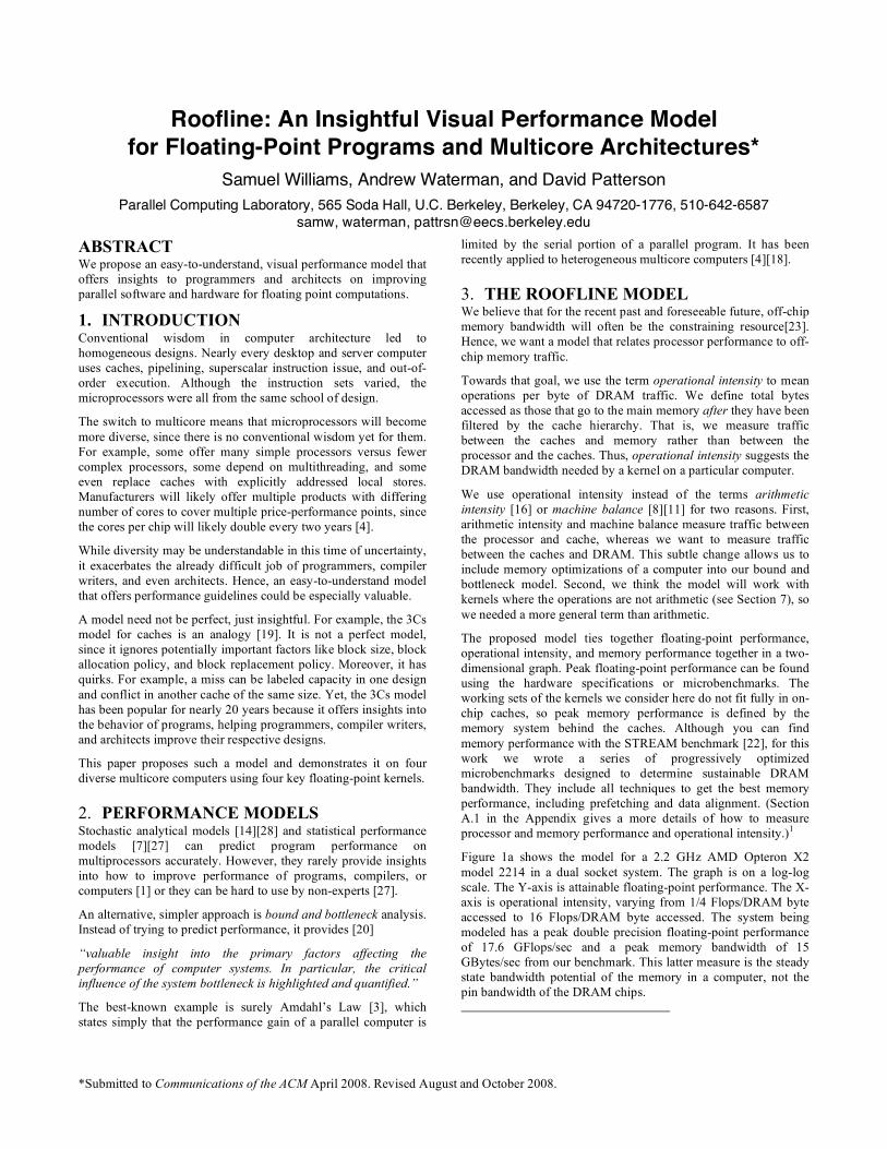
Figure 1a shows the model for a 2.2 GHz AMD Opteron X2 model 2214 in a dual socket system. The graph is on a log-log scale. The Y-axis is attainable floating-point performance. The X-axis is operational intensity, varying from 1/4 Flops/DRAM byte accessed to 16 Flops/DRAM byte accessed. The system being modeled has a peak double precision floating-point performance of 17.6 GFlops/sec and a peak memory bandwidth of 15 GBytes/sec from our benchmark. This latter measure is the steady state bandwidth potential of the memory in a computer, not the pin bandwidth of the DRAM chips.

2

We can plot a horizontal line showing peak floating-point performance of the computer. Obviously, the actual floating-point performance of a floating-point kernel can be no higher than the horizontal line, since that is a hardware limit.

How could we plot the peak memory performance? Since X-axis is GFlops per byte and the Y-axis is GFlops per second, bytes per second—which equals (GFlops/second)/(GFlops/byte)—is just a line at a 45-degree angle in this figure. Hence, we can plot a second line that gives the maximum floating-point performance that the memory system of that computer can support for a given operational intensity. This formula drives the two performance limits in the graph in Figure 1a:

Attainable GFlops/sec = Min(Peak Floating Point Performance, Peak Memory Bandwidth x Operational Intensity)

These two lines intersect at the point of peak computational performance and peak memory bandwidth. Note that these limits are created once per multicore computer, not once per kernel.

For a given kernel, we can find a point on the X-axis based on its operational intensity. If we draw a (pink dashed) vertical line through that point, the performance of the kernel on that computer must lie somewhere along that line.

The horizontal and diagonal lines give this bound model its name. The Roofline sets an upper bound on performance of a kernel depending on its operational intensity. If we think of operational intensity as a column that hits the roof, either it hits the flat part of the roof, which means performance is compute bound, or it hits the slanted part of the roof, which means performance is ultimately memory bound. In Figure 1a, a kernel with operational intensity 2 is compute bound and a kernel with operational intensity 1 is memory bound. Given a Roofline, you can use it repeatedly on different kernels, since the Roofline doesn’t vary.

Note that the ridge point, where the diagonal and horizontal roofs meet, offers an insight into the overall performance of the computer. The x-coordinate of the ridge point is the minimum operational intensity required to achieve maximum performance. If the ridge point is far to the right, then only kernels with very high operational intensity can achieve the maximum performance of that computer. If it is far to the left, then almost any kernel can potentially hit the maximum performance. As we shall see (Section 6.3.5), the ridge point suggests the level of difficulty for programmers and compiler writers to achieve peak performance.

To illustrate, let’s compare the Opteron X2 with two cores in Figure 1a to its successor, the Opteron X4 with four cores. To simplify board design, they share the same socket. Hence, they have the same DRAM channels and can thus have the same peak memory bandwidth, although the prefetching is better in the X4. In addition to doubling the number of cores, the X4 also has twice the peak floating-point performance per core: X4 cores can issue two floating-point SSE2 instructions per clock cycle while X2 cores can issue two every other clock. As the clock rate is slightly faster—2.2 GHz for X2 versus 2.3 GHz for X4—the X4 has slightly more than four times the peak floating-point performance of the X2 with the same memory bandwidth.

Figure 1b compares the Roofline models for both systems. As expected, the ridge point shifts right from 1.0 in the Opteron X2 to 4.4 in the Opteron X4. Hence, to see a performance gain in the X4, kernels need an operational intensity higher than 1.

Figure 1. Roofline Model for (a) AMD Opteron X2 on left and (b) Opteron X2 vs. Opteron X4 on right.

4. ADDING CEILINGS TO THE MODEL The Roofline model gives an upper bound to performance. Suppose your program is performing far below its Roofline. What optimizations should you perform, and in what order? Another advantage of bound and bottleneck analysis is [20]

“a number of alternatives can be treated together, with a single bounding analysis providing useful information about them all.”

We leverage this insight to add multiple ceilings to the Roofline model to guide which optimizations to perform, which are similar to the guidelines that loop balance gives the compiler. We can think of each of these optimizations as a “performance ceiling” below the appropriate Roofline, meaning that you cannot break through a ceiling without performing the associated optimization.

For example, to reduce computational bottlenecks on the Opteron X2, two optimizations can help almost any kernel:

1. Improve instruction level parallelism (ILP) and apply SIMD. For superscalar architectures, the highest performance comes when fetching, executing, and committing the maximum number of instructions per clock cycle. The goal here is to improve the code from the compiler to increase ILP. The highest performance comes from completely covering the functional unit latency. One way is by unrolling loops. For the x86-based architectures, another way is using floating-point SIMD instructions whenever possible, since an SIMD instruction operates on pairs of adjacent operands.

2. Balance floating-point operation mix. The best performance requires that a significant fraction of the instruction mix be floating-point operations (see Section 7). Peak floating-point performance typically also requires an equal number of simultaneous floating-point additions and multiplications, since many computers have multiply-add instructions or because they have an equal number of adders and multipliers.

To reduce memory bottlenecks, three optimizations can help:

3. Restructure loops for unit stride accesses. Optimizing for unit stride memory accesses engages hardware prefetching, which significantly increases memory bandwidth.

4. Ensure memory affinity. Most microprocessors today include a memory controller on the same chip with the processors. If

3

the system has two multicore chips, then some addresses go to the DRAM local to one multicore chip and the rest must go over a chip interconnect to access the DRAM that is local to another chip. This latter case lowers performance. This optimization allocates data and the threads tasked to that data to the same memory-processor pair, so that the processors rarely have to access the memory attached to other chips.

5. Use software prefetching. Usually the highest performance requires keeping many memory operations in flight, which is easier to do via prefetching rather than waiting until the data is actually requested by the program. On some computers, software prefetching delivers more bandwidth than hardware prefetching alone.

Like the computational Roofline, the computational ceilings can come from an optimization manual [2], although it’s easy to imagine collecting the necessary parameters from simple microbenchmarks. The memory ceilings require running experiments on each computer to determine the gap between them (see Appendix A.1). The good news is that like the Roofline, the ceilings only need be measured once per multicore computer.

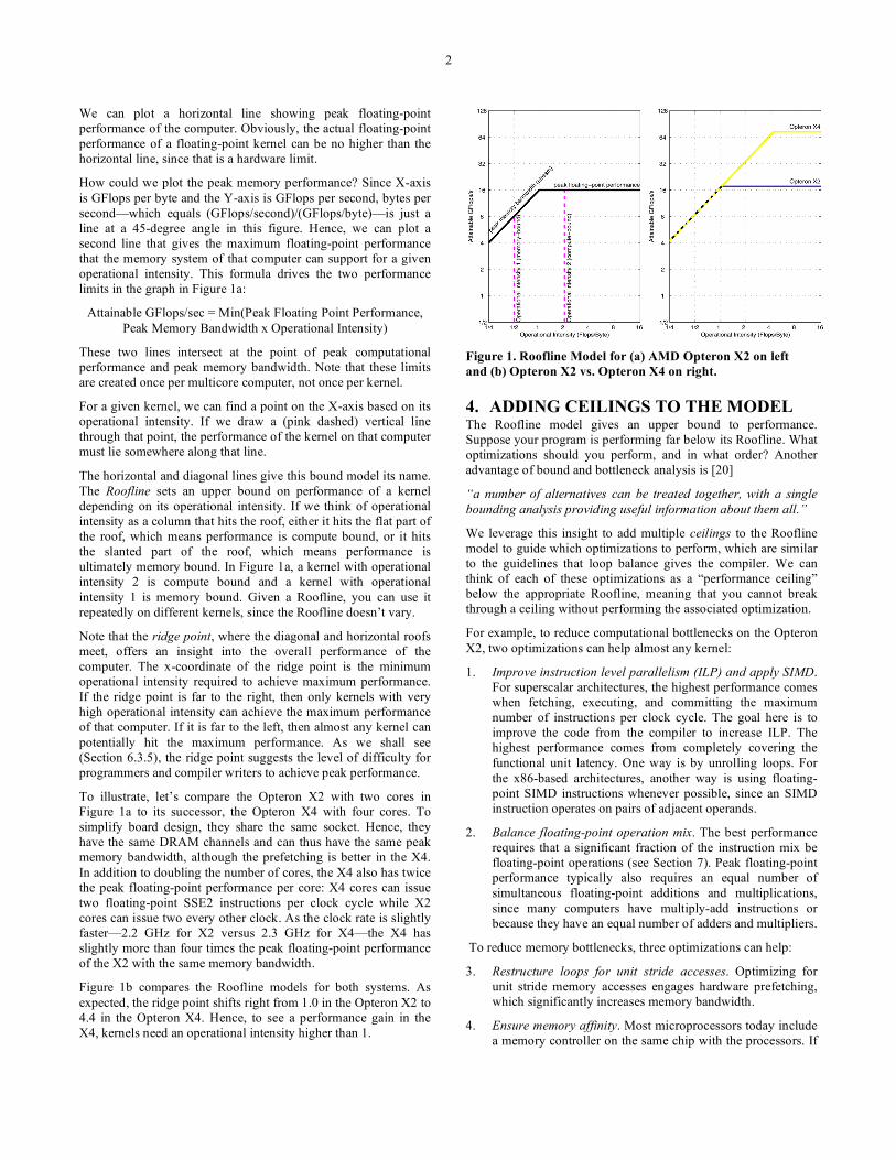
Figure 2 adds ceilings to the Roofline model in Figure 1a: Figure 2a shows the computational ceilings and Figure 2b the memory bandwidth ceilings. Although the higher ceilings are not labeled with lower optimizations, they are implied: to break through a ceiling, you need to have already broken through all the ones below. Figure 2a shows the computational “ceilings” of 8.8 GFlops/sec if the floating-point operation mix is imbalanced and

2.2 GFlops/sec if the optimizations to increase ILP or SIMD are also missing. Figure 2b shows the memory bandwidth ceilings of 11 GBytes/sec without software prefetching, 4.8 GBytes/sec without memory affinity optimizations as well, and 2.7 GBytes/sec with only unit stride optimizations.

Figure 2c combines the other two figures into a single graph. The operational intensity of a kernel determines the optimization region, and thus which optimizations to try. The middle of Figure 2c shows that the computational optimizations and the memory bandwidth optimizations overlap. The colors were picked to highlight that overlap. For example, Kernel 2 falls in the blue trapezoid on the right, which suggests working only on the computational optimizations. If a kernel fell in the yellow triangle on the lower left, the model would suggest trying just memory optimizations. Kernel 1 falls in the green (= yellow + blue) parallelogram in the middle, which suggests trying both types of optimizations. Note that the Kernel 1 vertical lines falls below the floating-point imbalance optimization, so optimization 2 may be skipped.

The ceilings of the Roofline model suggest which optimizations to perform. The height of the gap between a ceiling and the next higher one is the potential reward for trying that optimization. Thus, Figure 2 suggests that optimization 1, which improves ILP/SIMD, has a large potential benefit for improving computation on that computer, and optimization 4, which improves memory affinity, has a large potential benefit for improving memory bandwidth on that computer.

The order of the ceilings suggest the optimization order, so we rank the ceilings from bottom to top: those most likely to be realized by a compiler or with little effort by a programmer are at the bottom and those that are difficult to be implemented by a programmer or inherently lacking in a kernel are at the top. The one quirk is floating-point balance, since the actual mix is dependent on the kernel. For most kernels, achieving parity between multiplies and additions is very difficult, but for a few, parity is natural. One example is sparse matrix-vector multiplication. For that domain, we would place floating-point mix as the lowest ceiling, since it is inherent. Like the 3Cs model, as long as the Roofline model delivers on insights, it need not be perfect.

Figure 2. Roofline Model with Ceilings for Opteron X2.

4

5. Tying the 3Cs to Operational Intensity Operational intensity tells us which ceilings to look at. Thus far, we have been assuming that the operational intensity is fixed, but that is not really the case. For example, there are kernels where the operational intensity increases with problem size, such as for Dense Matrix and FFT problems.

Clearly, caches affect the number of accesses that go to memory, so optimizations that improve cache performance increase operational intensity. Hence, we can connect the 3Cs model to the Roofline model. Compulsory misses set the minimum memory traffic and hence the highest possible operational intensity. Memory traffic from conflict and capacity misses can considerably lower the operational intensity of a kernel, so we should try to eliminate such misses.

For example, we can reduce traffic from conflict misses by padding arrays to change cache line addressing. A second example is that some computers have a no-allocate store instruction, so stores go directly to memory and do not affect the caches. This optimization prevents loading a cache block with data to be overwritten, thereby reducing memory traffic. It also prevents displacing useful items in the cache with data that will not be read thereby saving conflict misses.

This shift right of operational intensity could put a kernel in a different optimization region. The advice is generally to improve operational intensity of the kernel before other optimizations.

6. DEMONSTRATION OF THE MODEL To demonstrate the utility of the model, we develop Roofline models for 4 recent multicore computers and then optimize 4 floating-point kernels. We then show that the ceilings and rooflines bound the achieved results for all computers and kernels.

6.1 Four Diverse Multicore Computers Given the lack of conventional wisdom for multicore architecture, it’s not surprising that there are as many different designs as there are chips. Table 1 lists the key characteristics of the four multicore computers of this section, which are all dual-socket systems.

The Intel Xeon uses relatively sophisticated processors, capable of executing two SIMD instructions per clock cycle that can each perform two double-precision floating-point operations. It is the only one of the four machines with a front side bus connecting to a common north bridge chip and memory controller. The other three have the memory controller on chip.

The Opteron X4 also uses sophisticated cores with high peak floating–point performance, but it is the only computer of the four with on-chip L3 caches. These two sockets communicate over separate, dedicated Hypertransport links, which makes it possible to build a “glueless” multi-chip system.

The Sun UltraSPARC T2+ uses relatively simple processors at a modest clock rate compared to the others, which allows it to have twice as many cores per chip. It is also highly multithreaded, with eight hardware-supported threads per core. It has the highest memory bandwidth of the four, for each chip has two dual-channel memory controllers that can drive four sets of DDR2/FBDIMMs.

The clock rate of IBM Cell QS20 is highest of the four multicores at 3.2 GHz. It is also most unusual. It is a heterogeneous design,

with a relatively simple PowerPC core and with eight SPEs (Synergistic Processing Elements) that have their own unique SIMD-style instruction set. Each SPE also has its own local memory instead of a cache. An SPE must transfer data from main memory into the local memory to operate on it and then back to main memory when it is completed. It uses DMA, which has some similarity to software prefetching. The lack of caches means porting programs to Cell is more challenging.

6.2 Four Diverse Floating-Point Kernels Rather than pick programs from some standard parallel benchmark suite such as Parsec [5] or Splash-2 [30], we were inspired by the work of Phil Colella [10]. This expert in scientific computing has identified seven numerical methods that he believes will be important for science and engineering for at least the next decade. Because he picked seven, they have become known as the Seven Dwarfs. The dwarfs are specified at a high level of abstraction to allow reasoning about their behavior across a broad range of implementations. The widely read “Berkeley View” report [4] found that if the data types were changed from floating point to integer, those same dwarfs could also be found in many other programs. Note that the claim is not that the dwarfs are easy to parallelize. The claim is that they will be important to computing in most current and future applications, so designers are advised to make sure they run well on systems that they create, whether or not their creations are parallel.

One advantage of using these higher-level descriptions of programs is that we are not tied to code that may have been written originally to optimize an old computer to evaluate future systems. Another advantage of the restricted number is that we can create autotuners for each kernel that would search the space of alternatives to produce the best code for that multicore computer, including extensive cache optimizations [13].

With that background, Table 2 lists the four kernels from the dwarfs that we use to demonstrate the Roofline Model on the four multicore computers of Table 1. The auto-tuning for this section is from [12], [25] and [26].

For these kernels, there is sufficient parallelism to utilize all the cores and threads and to keep them load balanced. (Appendix A.2 describes how to handle cases when load is not balanced.)

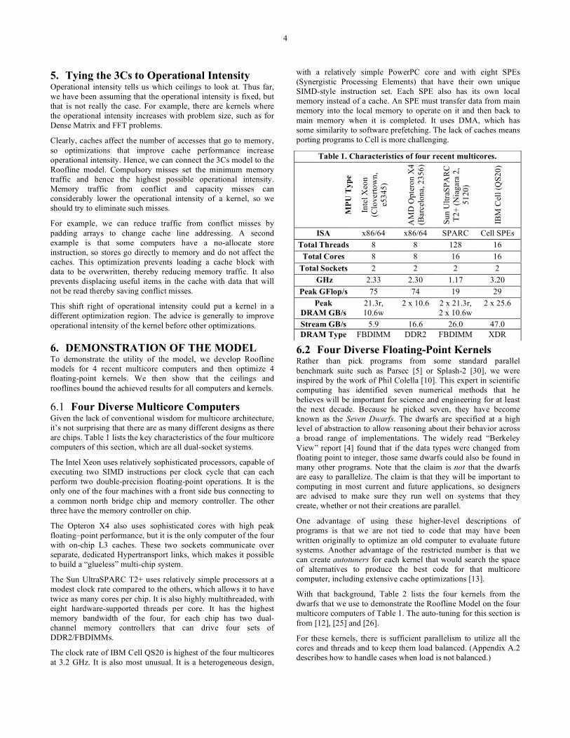
Table 1. Characteristics of four recent multicores.

MPU

Typ

e

Inte

l Xeo

n (C

love

rtow

n,

e534

5)

AM

D O

pter

on X

4 (B

arce

lona

, 235

6)

Sun

Ultr

aSPA

RC

T2

+ (N

iaga

ra 2

, 51

20)

IBM

Cel

l (Q

S20)

ISA x86/64 x86/64 SPARC Cell SPEs Total Threads 8 8 128 16

Total Cores 8 8 16 16 Total Sockets 2 2 2 2

GHz 2.33 2.30 1.17 3.20 Peak GFlop/s 75 74 19 29

Peak DRAM GB/s

21.3r, 10.6w

2 x 10.6 2 x 21.3r, 2 x 10.6w

2 x 25.6

Stream GB/s 5.9 16.6 26.0 47.0 DRAM Type FBDIMM DDR2 FBDIMM XDR

5

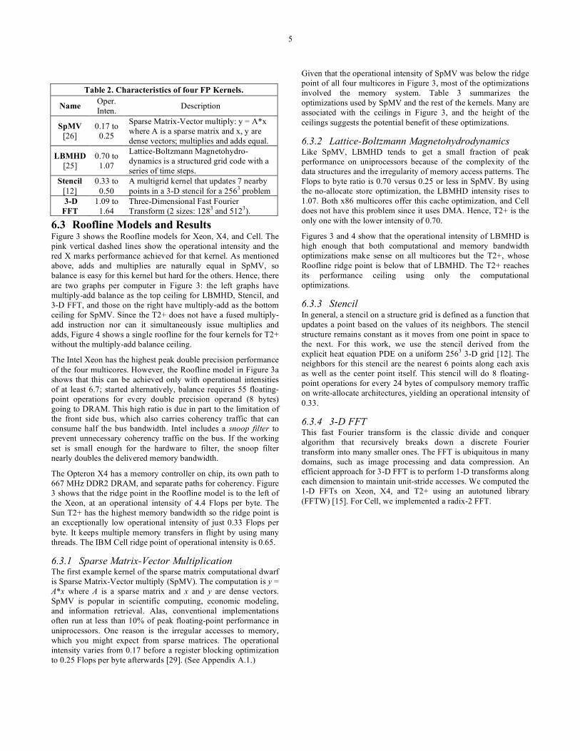
Table 2. Characteristics of four FP Kernels.

Name Oper. Inten. Description

SpMV [26]

0.17 to 0.25

Sparse Matrix-Vector multiply: y = A*x where A is a sparse matrix and x, y are dense vectors; multiplies and adds equal.

LBMHD [25]

0.70 to 1.07

Lattice-Boltzmann Magnetohydro- dynamics is a structured grid code with a series of time steps.

Stencil [12]

0.33 to 0.50

A multigrid kernel that updates 7 nearby points in a 3-D stencil for a 2563 problem

3-D FFT

1.09 to 1.64

Three-Dimensional Fast Fourier Transform (2 sizes: 1283 and 5123).

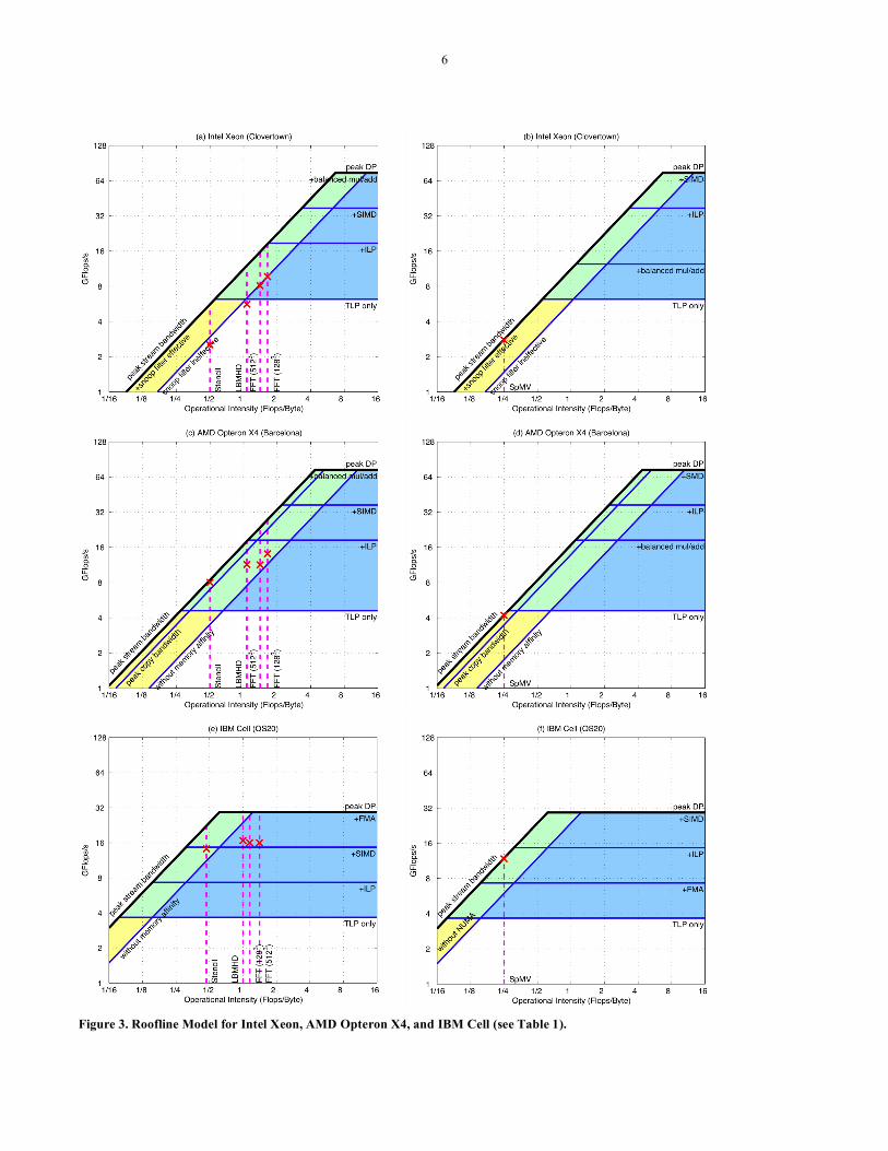
6.3 Roofline Models and Results Figure 3 shows the Roofline models for Xeon, X4, and Cell. The pink vertical dashed lines show the operational intensity and the red X marks performance achieved for that kernel. As mentioned above, adds and multiplies are naturally equal in SpMV, so balance is easy for this kernel but hard for the others. Hence, there are two graphs per computer in Figure 3: the left graphs have multiply-add balance as the top ceiling for LBMHD, Stencil, and 3-D FFT, and those on the right have multiply-add as the bottom ceiling for SpMV. Since the T2+ does not have a fused multiply-add instruction nor can it simultaneously issue multiplies and adds, Figure 4 shows a single roofline for the four kernels for T2+ without the multiply-add balance ceiling.

The Intel Xeon has the highest peak double precision performance of the four multicores. However, the Roofline model in Figure 3a shows that this can be achieved only with operational intensities of at least 6.7; started alternatively, balance requires 55 floating-point operations for every double precision operand (8 bytes) going to DRAM. This high ratio is due in part to the limitation of the front side bus, which also carries coherency traffic that can consume half the bus bandwidth. Intel includes a snoop filter to prevent unnecessary coherency traffic on the bus. If the working set is small enough for the hardware to filter, the snoop filter nearly doubles the delivered memory bandwidth.

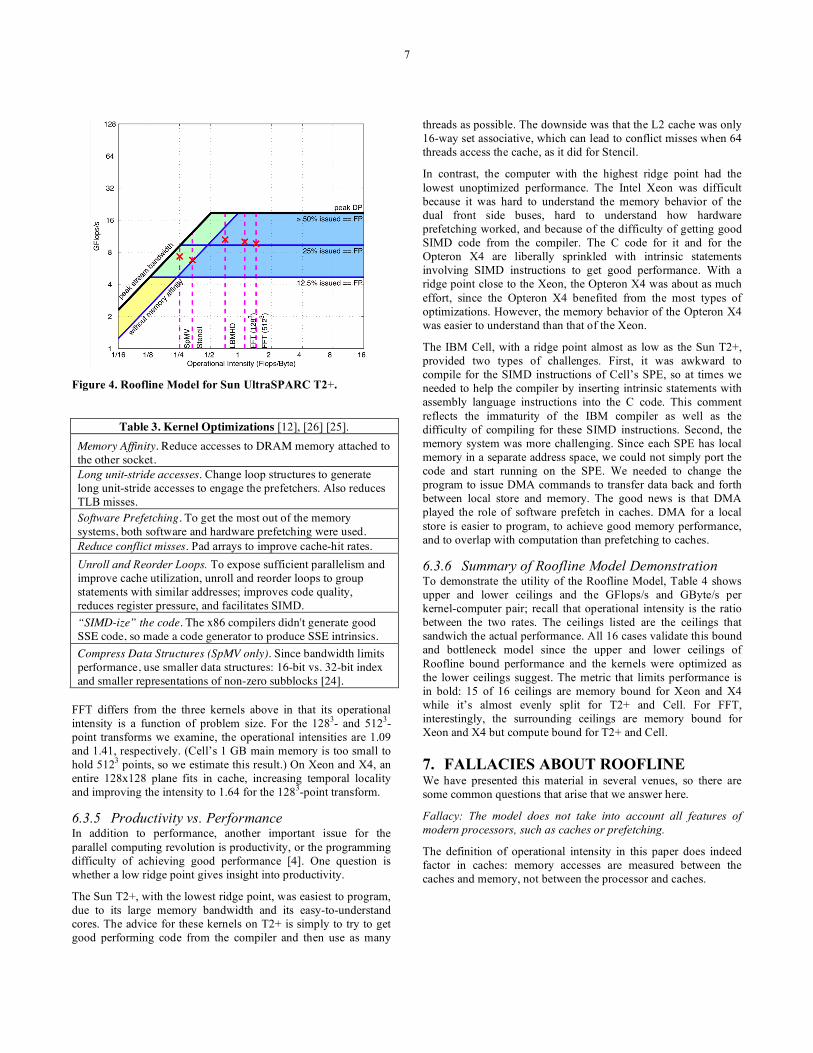
The Opteron X4 has a memory controller on chip, its own path to 667 MHz DDR2 DRAM, and separate paths for coherency. Figure 3 shows that the ridge point in the Roofline model is to the left of the Xeon, at an operational intensity of 4.4 Flops per byte. The Sun T2+ has the highest memory bandwidth so the ridge point is an exceptionally low operational intensity of just 0.33 Flops per byte. It keeps multiple memory transfers in flight by using many threads. The IBM Cell ridge point of operational intensity is 0.65.

6.3.1 Sparse Matrix-Vector Multiplication The first example kernel of the sparse matrix computational dwarf is Sparse Matrix-Vector multiply (SpMV). The computation is y = A*x where A is a sparse matrix and x and y are dense vectors. SpMV is popular in scientific computing, economic modeling, and information retrieval. Alas, conventional implementations often run at less than 10% of peak floating-point performance in uniprocessors. One reason is the irregular accesses to memory, which you might expect from sparse matrices. The operational intensity varies from 0.17 before a register blocking optimization to 0.25 Flops per byte afterwards [29]. (See Appendix A.1.)

Given that the operational intensity of SpMV was below the ridge point of all four multicores in Figure 3, most of the optimizations involved the memory system. Table 3 summarizes the optimizations used by SpMV and the rest of the kernels. Many are associated with the ceilings in Figure 3, and the height of the ceilings suggests the potential benefit of these optimizations.

6.3.2 Lattice-Boltzmann Magnetohydrodynamics Like SpMV, LBMHD tends to get a small fraction of peak performance on uniprocessors because of the complexity of the data structures and the irregularity of memory access patterns. The Flops to byte ratio is 0.70 versus 0.25 or less in SpMV. By using the no-allocate store optimization, the LBMHD intensity rises to 1.07. Both x86 multicores offer this cache optimization, and Cell does not have this problem since it uses DMA. Hence, T2+ is the only one with the lower intensity of 0.70.

Figures 3 and 4 show that the operational intensity of LBMHD is high enough that both computational and memory bandwidth optimizations make sense on all multicores but the T2+, whose Roofline ridge point is below that of LBMHD. The T2+ reaches its performance ceiling using only the computational optimizations.

6.3.3 Stencil In general, a stencil on a structure grid is defined as a function that updates a point based on the values of its neighbors. The stencil structure remains constant as it moves from one point in space to the next. For this work, we use the stencil derived from the explicit heat equation PDE on a uniform 2563 3-D grid [12]. The neighbors for this stencil are the nearest 6 points along each axis as well as the center point itself. This stencil will do 8 floating-point operations for every 24 bytes of compulsory memory traffic on write-allocate architectures, yielding an operational intensity of 0.33.

6.3.4 3-D FFT This fast Fourier transform is the classic divide and conquer algorithm that recursively breaks down a discrete Fourier transform into many smaller ones. The FFT is ubiquitous in many domains, such as image processing and data compression. An efficient approach for 3-D FFT is to perform 1-D transforms along each dimension to maintain unit-stride accesses. We computed the 1-D FFTs on Xeon, X4, and T2+ using an autotuned library (FFTW) [15]. For Cell, we implemented a radix-2 FFT.

6

Figure 3. Roofline Model for Intel Xeon, AMD Opteron X4, and IBM Cell (see Table 1).

7

Figure 4. Roofline Model for Sun UltraSPARC T2+.

Table 3. Kernel Optimizations [12], [26] [25]. Memory Affinity. Reduce accesses to DRAM memory attached to the other socket. Long unit-stride accesses. Change loop structures to generate long unit-stride accesses to engage the prefetchers. Also reduces TLB misses. Software Prefetching. To get the most out of the memory systems, both software and hardware prefetching were used. Reduce conflict misses. Pad arrays to improve cache-hit rates. Unroll and Reorder Loops. To expose sufficient parallelism and improve cache utilization, unroll and reorder loops to group statements with similar addresses; improves code quality, reduces register pressure, and facilitates SIMD. “SIMD-ize” the code. The x86 compilers didn't generate good SSE code, so made a code generator to produce SSE intrinsics. Compress Data Structures (SpMV only). Since bandwidth limits performance, use smaller data structures: 16-bit vs. 32-bit index and smaller representations of non-zero subblocks [24].

FFT differs from the three kernels above in that its operational intensity is a function of problem size. For the 1283- and 5123-point transforms we examine, the operational intensities are 1.09 and 1.41, respectively. (Cell’s 1 GB main memory is too small to hold 5123 points, so we estimate this result.) On Xeon and X4, an entire 128x128 plane fits in cache, increasing temporal locality and improving the intensity to 1.64 for the 1283-point transform.

6.3.5 Productivity vs. Performance In addition to performance, another important issue for the parallel computing revolution is productivity, or the programming difficulty of achieving good performance [4]. One question is whether a low ridge point gives insight into productivity.

The Sun T2+, with the lowest ridge point, was easiest to program, due to its large memory bandwidth and its easy-to-understand cores. The advice for these kernels on T2+ is simply to try to get good performing code from the compiler and then use as many

threads as possible. The downside was that the L2 cache was only 16-way set associative, which can lead to conflict misses when 64 threads access the cache, as it did for Stencil.

In contrast, the computer with the highest ridge point had the lowest unoptimized performance. The Intel Xeon was difficult because it was hard to understand the memory behavior of the dual front side buses, hard to understand how hardware prefetching worked, and because of the difficulty of getting good SIMD code from the compiler. The C code for it and for the Opteron X4 are liberally sprinkled with intrinsic statements involving SIMD instructions to get good performance. With a ridge point close to the Xeon, the Opteron X4 was about as much effort, since the Opteron X4 benefited from the most types of optimizations. However, the memory behavior of the Opteron X4 was easier to understand than that of the Xeon.

The IBM Cell, with a ridge point almost as low as the Sun T2+, provided two types of challenges. First, it was awkward to compile for the SIMD instructions of Cell’s SPE, so at times we needed to help the compiler by inserting intrinsic statements with assembly language instructions into the C code. This comment reflects the immaturity of the IBM compiler as well as the difficulty of compiling for these SIMD instructions. Second, the memory system was more challenging. Since each SPE has local memory in a separate address space, we could not simply port the code and start running on the SPE. We needed to change the program to issue DMA commands to transfer data back and forth between local store and memory. The good news is that DMA played the role of software prefetch in caches. DMA for a local store is easier to program, to achieve good memory performance, and to overlap with computation than prefetching to caches.

6.3.6 Summary of Roofline Model Demonstration To demonstrate the utility of the Roofline Model, Table 4 shows upper and lower ceilings and the GFlops/s and GByte/s per kernel-computer pair; recall that operational intensity is the ratio between the two rates. The ceilings listed are the ceilings that sandwich the actual performance. All 16 cases validate this bound and bottleneck model since the upper and lower ceilings of Roofline bound performance and the kernels were optimized as the lower ceilings suggest. The metric that limits performance is in bold: 15 of 16 ceilings are memory bound for Xeon and X4 while it’s almost evenly split for T2+ and Cell. For FFT, interestingly, the surrounding ceilings are memory bound for Xeon and X4 but compute bound for T2+ and Cell.

7. FALLACIES ABOUT ROOFLINE We have presented this material in several venues, so there are some common questions that arise that we answer here.

Fallacy: The model does not take into account all features of modern processors, such as caches or prefetching.

The definition of operational intensity in this paper does indeed factor in caches: memory accesses are measured between the caches and memory, not between the processor and caches.

8

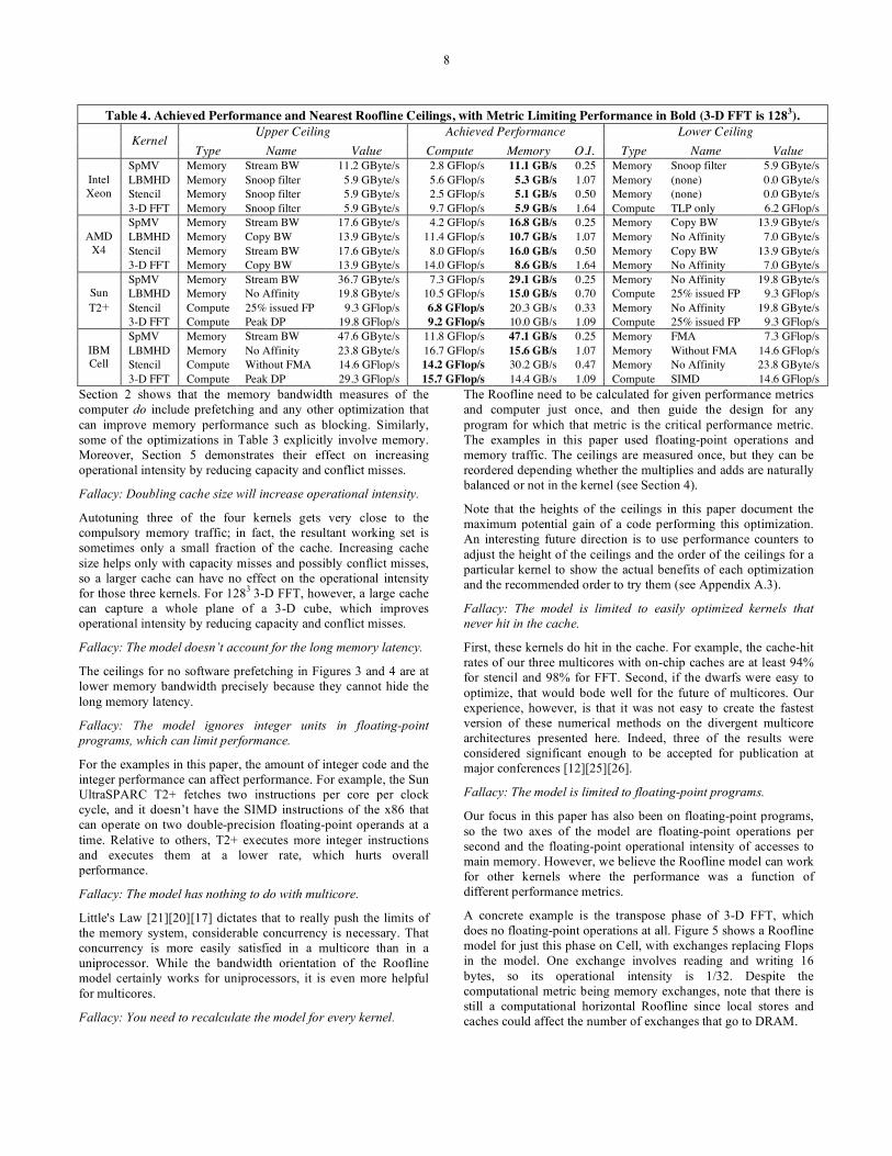
Table 4. Achieved Performance and Nearest Roofline Ceilings, with Metric Limiting Performance in Bold (3-D FFT is 1283). Upper Ceiling Achieved Performance Lower Ceiling

Kernel

Type Name Value Compute Memory O.I. Type Name Value SpMV Memory Stream BW 11.2 GByte/s 2.8 GFlop/s 11.1 GB/s 0.25 Memory Snoop filter 5.9 GByte/s LBMHD Memory Snoop filter 5.9 GByte/s 5.6 GFlop/s 5.3 GB/s 1.07 Memory (none) 0.0 GByte/s Stencil Memory Snoop filter 5.9 GByte/s 2.5 GFlop/s 5.1 GB/s 0.50 Memory (none) 0.0 GByte/s

Intel Xeon

3-D FFT Memory Snoop filter 5.9 GByte/s 9.7 GFlop/s 5.9 GB/s 1.64 Compute TLP only 6.2 GFlop/s SpMV Memory Stream BW 17.6 GByte/s 4.2 GFlop/s 16.8 GB/s 0.25 Memory Copy BW 13.9 GByte/s LBMHD Memory Copy BW 13.9 GByte/s 11.4 GFlop/s 10.7 GB/s 1.07 Memory No Affinity 7.0 GByte/s Stencil Memory Stream BW 17.6 GByte/s 8.0 GFlop/s 16.0 GB/s 0.50 Memory Copy BW 13.9 GByte/s

AMD X4

3-D FFT Memory Copy BW 13.9 GByte/s 14.0 GFlop/s 8.6 GB/s 1.64 Memory No Affinity 7.0 GByte/s SpMV Memory Stream BW 36.7 GByte/s 7.3 GFlop/s 29.1 GB/s 0.25 Memory No Affinity 19.8 GByte/s LBMHD Memory No Affinity 19.8 GByte/s 10.5 GFlop/s 15.0 GB/s 0.70 Compute 25% issued FP 9.3 GFlop/s Stencil Compute 25% issued FP 9.3 GFlop/s 6.8 GFlop/s 20.3 GB/s 0.33 Memory No Affinity 19.8 GByte/s

Sun T2+

3-D FFT Compute Peak DP 19.8 GFlop/s 9.2 GFlop/s 10.0 GB/s 1.09 Compute 25% issued FP 9.3 GFlop/s SpMV Memory Stream BW 47.6 GByte/s 11.8 GFlop/s 47.1 GB/s 0.25 Memory FMA 7.3 GFlop/s LBMHD Memory No Affinity 23.8 GByte/s 16.7 GFlop/s 15.6 GB/s 1.07 Memory Without FMA 14.6 GFlop/s Stencil Compute Without FMA 14.6 GFlop/s 14.2 GFlop/s 30.2 GB/s 0.47 Memory No Affinity 23.8 GByte/s

IBM Cell

3-D FFT Compute Peak DP 29.3 GFlop/s 15.7 GFlop/s 14.4 GB/s 1.09 Compute SIMD 14.6 GFlop/s Section 2 shows that the memory bandwidth measures of the computer do include prefetching and any other optimization that can improve memory performance such as blocking. Similarly, some of the optimizations in Table 3 explicitly involve memory. Moreover, Section 5 demonstrates their effect on increasing operational intensity by reducing capacity and conflict misses.

Fallacy: Doubling cache size will increase operational intensity.

Autotuning three of the four kernels gets very close to the compulsory memory traffic; in fact, the resultant working set is sometimes only a small fraction of the cache. Increasing cache size helps only with capacity misses and possibly conflict misses, so a larger cache can have no effect on the operational intensity for those three kernels. For 1283 3-D FFT, however, a large cache can capture a whole plane of a 3-D cube, which improves operational intensity by reducing capacity and conflict misses.

Fallacy: The model doesn’t account for the long memory latency.

The ceilings for no software prefetching in Figures 3 and 4 are at lower memory bandwidth precisely because they cannot hide the long memory latency.

Fallacy: The model ignores integer units in floating-point programs, which can limit performance.

For the examples in this paper, the amount of integer code and the integer performance can affect performance. For example, the Sun UltraSPARC T2+ fetches two instructions per core per clock cycle, and it doesn’t have the SIMD instructions of the x86 that can operate on two double-precision floating-point operands at a time. Relative to others, T2+ executes more integer instructions and executes them at a lower rate, which hurts overall performance.

Fallacy: The model has nothing to do with multicore.

Little's Law [21][20][17] dictates that to really push the limits of the memory system, considerable concurrency is necessary. That concurrency is more easily satisfied in a multicore than in a uniprocessor. While the bandwidth orientation of the Roofline model certainly works for uniprocessors, it is even more helpful for multicores.

Fallacy: You need to recalculate the model for every kernel.

The Roofline need to be calculated for given performance metrics and computer just once, and then guide the design for any program for which that metric is the critical performance metric. The examples in this paper used floating-point operations and memory traffic. The ceilings are measured once, but they can be reordered depending whether the multiplies and adds are naturally balanced or not in the kernel (see Section 4).

Note that the heights of the ceilings in this paper document the maximum potential gain of a code performing this optimization. An interesting future direction is to use performance counters to adjust the height of the ceilings and the order of the ceilings for a particular kernel to show the actual benefits of each optimization and the recommended order to try them (see Appendix A.3).

Fallacy: The model is limited to easily optimized kernels that never hit in the cache.

First, these kernels do hit in the cache. For example, the cache-hit rates of our three multicores with on-chip caches are at least 94% for stencil and 98% for FFT. Second, if the dwarfs were easy to optimize, that would bode well for the future of multicores. Our experience, however, is that it was not easy to create the fastest version of these numerical methods on the divergent multicore architectures presented here. Indeed, three of the results were considered significant enough to be accepted for publication at major conferences [12][25][26].

Fallacy: The model is limited to floating-point programs.

Our focus in this paper has also been on floating-point programs, so the two axes of the model are floating-point operations per second and the floating-point operational intensity of accesses to main memory. However, we believe the Roofline model can work for other kernels where the performance was a function of different performance metrics.

A concrete example is the transpose phase of 3-D FFT, which does no floating-point operations at all. Figure 5 shows a Roofline model for just this phase on Cell, with exchanges replacing Flops in the model. One exchange involves reading and writing 16 bytes, so its operational intensity is 1/32. Despite the computational metric being memory exchanges, note that there is still a computational horizontal Roofline since local stores and caches could affect the number of exchanges that go to DRAM.

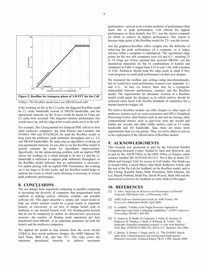
9

Figure 5. Roofline for transpose phase of 3-D FFT for the Cell

Fallacy: The Roofline model must use DRAM bandwidth.

If the working set fits in the L2 cache, the diagonal Roofline could be L2 cache bandwidth instead of DRAM bandwidth, and the operational intensity on the X-axis would be based on Flops per L2 cache byte accessed. The diagonal memory performance line would move up, and the ridge point would surely move to the left.

For example, Jike Chong ported two financial PDE solvers to four other multicore computers: the Intel Penryn and Larrabee and NVIDIA G80 and GTX280.[9] He used the Roofline model to keep track the platforms' peak arithmetic throughput and L1, L2, and DRAM bandwidths. By analyzing an algorithm's working set and operational intensity, he was able to use the Roofline model to quickly estimate the needs for algorithmic improvements. Specifically, for the option-pricing problem with an implicit PDE solver, the working set is small enough to fit into L1 and the L1 bandwidth is sufficient to support peak arithmetic throughput, so the Roofline model indicates that no optimization is necessary. For option pricing with an explicit PDE formulation, the working set is too large to fit into cache, and the Roofline model helps to indicate the extent to which cache blocking is necessary to extract peak arithmetic performance.

8. CONCLUSIONS The sea change from sequential computing to parallel computing is increasing the diversity of computers that programmers must confront in making correct, efficient, scalable, and portable software [4]. This paper describes a simple and visual model to help see which systems would be a good match to important kernels, or conversely, to see how to change kernel code or hardware to run desired kernels well. For floating-point kernels that do not fit completely in caches, we showed how operational intensity—the number of floating point operations per byte transferred from DRAM—is an important parameter for both the kernels and the multicore computers.

We applied the model to four kernels from the seven dwarfs [10][4] to four recent multicore designs: the AMD Opteron X4, Intel Xeon, IBM Cell, and Sun T2+. The ridge point—the minimum operational intensity to achieve maximum

performance—proved to be a better predictor of performance than clock rate or peak performance. Cell offered the highest performance on these kernels, but T2+ was the easiest computer on which to achieve its highest performance. One reason is because ridge point of the Roofline model for T2+ was the lowest.

Just the graphical Roofline offers insights into the difficulty of achieving the peak performance of a computer, as it makes obvious when a computer is imbalanced. The operational ridge points for the two x86 computers were 4.4 and 6.7—meaning 35 to 55 Flops per 8-byte operand that accesses DRAM—yet the operational intensities for the 16 combinations of kernels and computers in Table 4 ranged from 0.25 to just 1.64, with a median of 0.60. Architects should keep the ridge point in mind if they want programs to reach peak performance on their new designs.

We measured the roofline and ceilings using microbenchmarks, but we could have used performance counters (see Appendix A.1 and A.3). In fact, we believe there may be a synergistic relationship between performance counters and the Roofline model. The requirements for automatic creation of a Roofline model could guide the designer as to which metrics should be collected when faced with literally hundreds of candidates but a limited hardware budget. [6]

We believe Roofline models can offer insights to other types of multicore systems such as vector processors and GPUs (Graphical Processing Units); other kernels such as sort and ray tracing; other computational metrics such as pair-wise sorts per second and frames per second; and other traffic metrics such as L3 cache bandwidth and I/O bandwidth. Alas, there are many more opportunities than we can pursue. Thus, we invite others to join us in the exploration of the effectiveness of Roofline models.

9. ACKNOWLEDGMENTS This research was sponsored in part by the Universal Parallel Computing Research Center, funded by Intel and Microsoft, and in part by the ASCR Office in the DOE Office of Science under contract number DE-AC02-05CH11231. We’d like to thank FZ-Jülich and Georgia Tech for access to Cell blades. Our thanks go to Joseph Gebis, Leonid Oliker, John Shalf, Katherine Yelick, and the rest of the Par Lab for feedback on the Roofline model, and to Jike Chong, Kaushik Datta, Mark Hoemmen, Matt Johnson, Jae Lee, Rajesh Nishtala, Heidi Pan, David Wessel, Mark Hill and the anonymous reviewers for feedback on early drafts of this paper.

10. REFERENCES [1] V. Adve, Analyzing the Behavior and Performance of Parallel

Programs, PhD thesis, Univ. of Wisconsin, 1993.

[2] AMD, Software Optimization Guide for AMD Family 10h Processors, Publication 40546, April 2008.

[3] G. Amdahl, “Validity of the Single Processor Approach to Achieving Large-Scale Computing Capabilities,” AFIPS Conference Proceedings 30(1967), 483-485.

[4] K. Asanovic, R. Bodik, B. Catanzaro, J. Gebis, K. Keutzer, D. Patterson, W. Plishker, J. Shalf, S. Williams, K. Yelick. “The landscape of parallel computing research: A view from Berkeley.” Tech. Rep. UCB/EECS-2006-183, EECS, U.C. Berkeley, Dec 2006.

[5] C. Bienia,. S. Kumar, J. Singh, and K. Li. “The PARSEC Bench-mark Suite: Characterization and Architectural Implications,” Princeton University Technical Report TR-81 1-008, January 2008.

10

[6] S. Bird et al, “A Case for Sensible Performance Counters,” submitted to the First USENIX Workshop on Hot Topics in Parallelism (HotPar ’09), Berkeley CA, March 2009.

[7] E. Boyd, W. Azeem, H. Lee, T. Shih, S. Hung, and E. Davidson, “A Hierarchical Approach to Modeling and Improving the Performance of Scientific Applications on the KSR1,” Proc. 1994 Int’l Conf. on Parallel Processing, vol. 3, pp. 188-192, 1994.

[8] D. Callahan, J. Cocke, and K. Kennedy. “Estimating interlock and improving balance for pipelined machines,” J. Parallel Distrb. Comput. 5, 334-358. 1988.

[9] J. Chong, Private Communication, 2008.

[10] P. Colella, “Defining Software Requirements for Scientific Computing,” presentation, 2004.

[11] S. Carr and K. Kennedy, “Improving the Ratio of Memory Operations to Floating-Point Operations in Loops,” ACM TOPLAS 16(4) (Nov. 1994).

[12] K. Datta, M. Murphy, V. Volkov, S. Williams, J. Carter, L. Oliker, D. Patterson, J Shalf, K. Yelick, “Stencil Computation Optimization and Autotuning on State-of-the-Art Multicore Architectures,” Supercomputing (SC08), 2008.

[13] J. Demmel, J. Dongarra, V. Eijkhout, E. Fuentes, A. Petitet, R. Vuduc, R. Whaley, and K. Yelick, “Self Adapting Linear Algebra Algorithms and Software,” Proc. IEEE: Special Issue on Program Generation, Optimization, and Adaptation, 93 (2) 2005.

[14] M. Dubois and F. A. Briggs, “Performance of Synchronized Iterative Processes in Multiprocessor Systems,” IEEE Trans. on Software Engineering SE-8, 4 (July 1982), 419-431.

[15] M. Frigo and S. Johnson, "The Design and Implementation of FFTW3," Proc. IEEE: Special Issue on Program Generation, Optimization, and Platform Adaptation. 93 (2) 2005.

[16] M. Harris, "Mapping Computational Concepts to GPUs," ACM SIGGRAPH Tutorials, Chapter 31, 2005.

[17] J. Hennessy and D. Patterson, Computer Architecture: A Quantitative Approach, 4th ed., Boston, MA: Morgan Kaufmann Publishers, 2007.

[18] M. Hill and M. Marty, “Amdahl's Law in the Multicore Era,” IEEE Computer, July 2008.

[19] M. Hill and A. Smith, "Evaluating Associativity in CPU Caches," IEEE Trans. on Computers, 38(12), pp. 1612-1630, Dec. 1989.

[20] E. Lazowska, J. Zahorjan, S. Graham, and K. Sevcik, Quantitative System Performance: Computer System Analysis Using Queueing Network Models, Prentice Hail, Upper Saddle River, NJ, 1984.

[21] J. D. C. Little, "A Proof of the Queueing Formula L = λ W" Operations Research, 9, 383-387 (1961).

[22] J. McCalpin, “STREAM: Sustainable Memory Bandwidth in High Performance Computers,” www.cs.virginia.edu/stream, 1995.

[23] D. Patterson, “Latency Lags Bandwidth,” 47:10, CACM, Oct. 2004.

[24] S. Williams, Autotuning Performance on Multicore Computers, PhD thesis, U.C. Berkeley, 2008.

[25] S. Williams, J. Carter, L. Oliker, J. Shalf, K. Yelick, "Lattice Boltzmann Simulation Optimization on Leading Multicore Platforms," Int’l Parallel & Distributed Processing Symposium (IPDPS), 2008.

[26] S. Williams, L. Oliker, R. Vuduc, J. Shalf, K. Yelick, J. Demmel, "Optimization of Sparse Matrix-Vector Multiplication on Emerging Multicore Platforms," Supercomputing (SC07), 2007.

[27] M. Tikir, L. Carrington, E. Strohmaier, A. Snavely, "A Genetic Algorithms Approach to Modeling the Performance of Memory-bound Computations," Supercomputing (SC07), 2007.

[28] A. Thomasian and P. Bay, “Analytic Queueing Network Models for Parallel Processing of Task Systems,” IEEE Trans. on Computers C-35, 12 (December 1986), 1045-1054.

[29] R. Vuduc, J. Demmel, K. Yelick, S. Kamil, R. Nishtala, and B. Lee. “Performance Optimizations and Bounds for Sparse Matrix-Vector Multiply,” Supercomputing (SC02), Nov. 2002.

[30] S. Woo, M. Ohara, E. Torrie, J-P Singh, and A. Gupta. “The SPLASH-2 programs: characterization and methodological considerations,” Proc. 22nd annual Int’l Symp. on Computer Architecture (ISCA '95), May 1995, 24 - 36.

Categories and Subject Descriptors B.8.2 [Performance And Reliability]: Performance Analysis and Design Aids, D.1.3 [Programming Techniques]: Concurrent Programming

General Terms Measurement, Performance, Experimentation

Keywords Performance model, Parallel Computer, Multicore Computer, Multiprocessor, Kernel, Sparse Matrix, Structured Grid, FFT, Stencil, AMD Opteron X4, AMD Barcelona, Intel Xeon, Intel Clovertown, IBM Cell, Sun UltraSPARC T2+, Sun Niagara 2

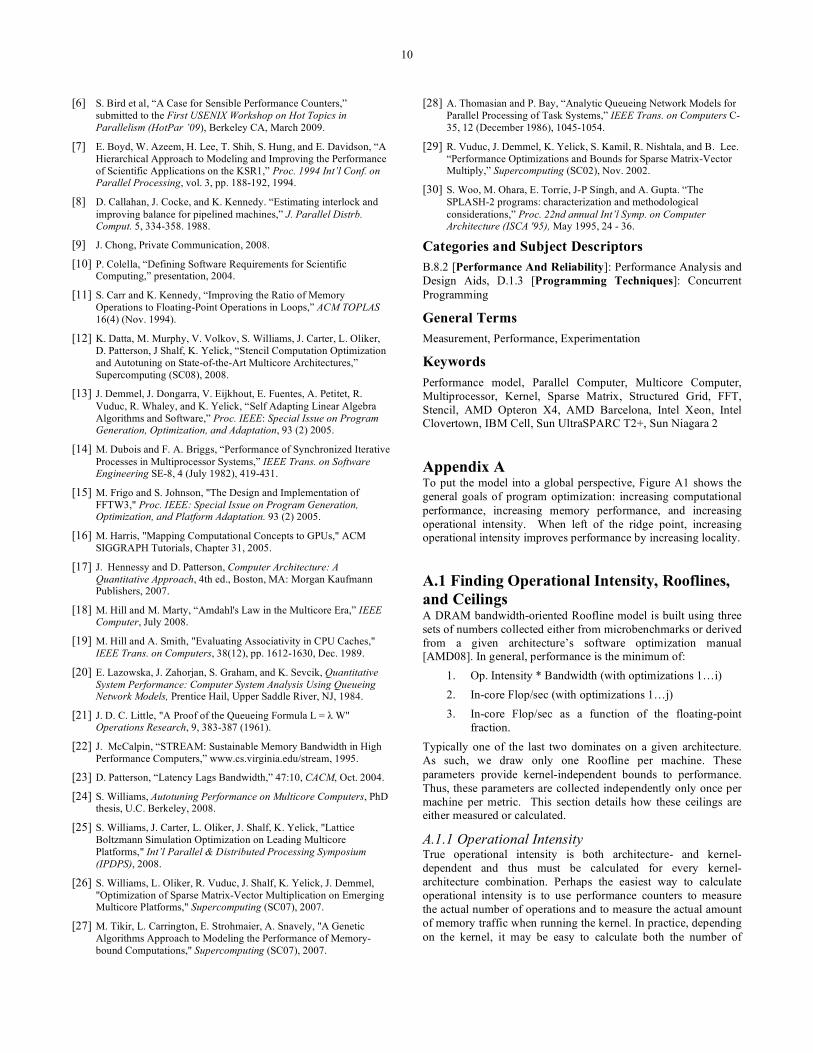
Appendix A To put the model into a global perspective, Figure A1 shows the general goals of program optimization: increasing computational performance, increasing memory performance, and increasing operational intensity. When left of the ridge point, increasing operational intensity improves performance by increasing locality.

A.1 Finding Operational Intensity, Rooflines, and Ceilings A DRAM bandwidth-oriented Roofline model is built using three sets of numbers collected either from microbenchmarks or derived from a given architecture’s software optimization manual [AMD08]. In general, performance is the minimum of:

1. Op. Intensity * Bandwidth (with optimizations 1…i) 2. In-core Flop/sec (with optimizations 1…j) 3. In-core Flop/sec as a function of the floating-point

fraction. Typically one of the last two dominates on a given architecture. As such, we draw only one Roofline per machine. These parameters provide kernel-independent bounds to performance. Thus, these parameters are collected independently only once per machine per metric. This section details how these ceilings are either measured or calculated.

A.1.1 Operational Intensity True operational intensity is both architecture- and kernel-dependent and thus must be calculated for every kernel-architecture combination. Perhaps the easiest way to calculate operational intensity is to use performance counters to measure the actual number of operations and to measure the actual amount of memory traffic when running the kernel. In practice, depending on the kernel, it may be easy to calculate both the number of

11

interesting operations and the minimum memory traffic by hand. Thus, one can bound the operational intensity.

A.1.2 Main Memory Bandwidth The first set of ceilings is main memory bandwidth with increasing optimization. Although the STREAM benchmark claims to report this bandwidth, it does not. It actually measures performance in terms of iterations per second, and then attempts to convert this to bandwidth based on the compulsory memory traffic on a non-write allocate architecture. This subtle, yet critical difference implies it cannot account for either conflict misses or the traffic associated with a fill on a write miss.

To correctly measure streaming bandwidth, we wrote a series of highly tuned versions of the STREAM benchmark that perform both a dot product and a copy. We pad arrays to avoid both bank and cache conflicts. We exploit the cache bypass instructions or increase the conversion constant to account for the fill traffic. The most naïve implementation allocates all data on one processor (no memory affinity), but is appropriately unrolled and padded. We proceed by correctly exploiting memory affinity and collect a new bandwidth. We then add software prefetching with an auto-tuned prefetch distance to the loop and measure bandwidth. Finally, we attempt to reduce the data set size to improve the effectiveness of a snoop filter. This provides a fourth bandwidth. We benchmark these individually, and define a new ceiling for each measured bandwidth.

A.1.3 In-Core Parallelism To estimate performance as a function of exploited in-core parallelism we rely on the appropriate software optimization manual [AMD08] for the architecture in question. In the long term, this is not a productive solution, as one would need to be very familiar with the breadth and evolution of all current and future architectures. However, for the purposes of this paper, no benchmark was necessary. Consider the following reduction:

y = x[1] + x[2] + x[3] + … + x[N]

We define thread-level-parallelism as the simplest parallelization optimization that could be applied. As such, the lowest ceiling is defined as the thread-level-parallelism-only ceiling. Each thread receives N/NThreads elements. We assume each thread executes a naïvely unrolled, yet dependent chain of scalar floating-point adds. Thus there is no instruction-, data-, or functional unit-level parallelism in the lowest ceiling. As such, the next add in the chain cannot be started until the previous has been completed. As a result, the latency of the floating-point pipeline is exposed. The resultant bound on throughput, irrespective of bandwidth, is calculated as:

Cores × Frequency × max(1, ThreadsPerCore/Latency)

Where ThreadsPerCore is the number of cores sharing a FPU within a core on a fine-grained multithreaded architecture. With enough threads, the FPU can be full utilized with ‘Latency’ threads hiding the FPU latency.

If the loop were further optimized by unrolling and maintaining several partial sums, then instruction-level parallelism is expressed. Thus, the next ceiling assumes sufficient per thread instruction-level parallelism to hide the functional unit latency. SIMD may not be included. Thus, the FPU would be completely occupied with scalar adds. The resultant throughput is:

Cores × Frequency

Third, we add data-level parallelism (SIMD) to the mix. Thus every two scalar add instructions into the partial sums becomes

Figure A1. General ways to improve performance in the Roofline model.

12

one SIMD add instruction in which two partial sums are stored in a SIMD register. For arbitrary SIMD register width, the resultant ceiling that incorporates thread-, instruction, and data-level parallelism is calculated as:

Cores × Frequency × SIMD width / SIMD throughput

The throughput term must be included as some architectures support SIMD instructions, but execute only one element per cycle. Thus, for an older Santa Rosa Opteron processor executing double precision SIMD instructions, the width is 2 FLOPs and throughput is one instruction per two cycles. Notice, the code does not perform any floating-point multiplies. However, if it were changed to:

y = y[1]*x[1] + y[2]*x[2] + y[3]*x[3] + … + y[N]*x[N]

Then there would be essentially a balance between the number of multiplies and adds. As such, we define peak in-core performance as the execution of unrolled and SIMDized fused multiply adds (FMAs); that is, the simultaneous execution of multiplies and adds. Architectures with a FMA or parallel add and multiply datapaths, the resultant bound on in-core performance is:

2 × Cores × Freq. × SIMD width / SIMD throughput

On Niagara2, where each core may issue only one scalar floating-point instruction per cycle, this is calculated as:

Cores × Frequency

Note that some computers, such as the IBM P5, have multiple, identical floating point datapaths. ILP would be used to satisfy both superscalar and deeply pipelined functional units. As such, they could get even more benefit from greater ILP than these equations show.

A.1.4 Instruction Mix All processors have limited instruction issue bandwidth. Their floating-point issue bandwidth is less than or equal to this bandwidth. As the non-floating-point fraction of issued instructions increases, eventually floating-point issue bandwidth will be starved to serve non-floating-point instructions. We calculate an orthogonal set of ceilings based on the floating-point fraction of the instruction mix assuming full exploitation of in-core parallelism. This approach is somewhat complicated as on Cell a double precision instruction stalls the issue unit for a further 6 cycles. We delineate the floating-point fraction in negative powers of 2. For a given architecture and kernel it is usually clear which in-core ceilings should be used. Such ceilings account for the potentially limited integer performance of these machines.

A.2 LOAD BALANCE AND ROOFLINE Load balance can loosely be categorized as either imbalance in the memory accesses or imbalance in the computation.

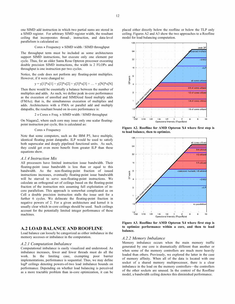
A.2.1 Computation Imbalance Computational imbalance is easily visualized and understood. As imbalance increases, fewer and fewer threads must do all the work. In the limiting case, exempting poor barrier implementations, performance is sequential. Thus, we may define logP ceilings denoting powers-of-two load imbalance bounds on performance. Depending on whether load balancing is perceived as a more tractable problem than in-core optimization, it can be

placed either directly below the roofline or below the TLP only ceiling. Figures A2 and A3 show the two approaches to a Roofline model for load balancing computation.

Figure A2. Roofline for AMD Opteron X4 where first step is to load balance, then to optimize.

Figure A3. Roofline for AMD Opteron X4 where first step is to optimize performance within a core, and then to load balance.

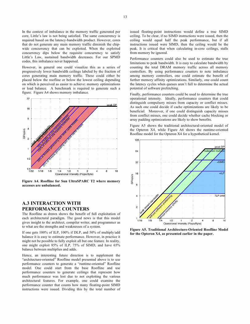
A.2.2 Memory Imbalance Memory imbalance occurs when the main memory traffic generated by one core is dramatically different than another or when some of the memory controllers are much more heavily loaded than others. Previously, we explored the latter in the case of memory affinity. When all of the data is located with one socket of a shared memory multiprocessor, there is a clear imbalance in the load on the memory controllers—the controllers of the other sockets are unused. In the context of the Roofline model, a bandwidth ceiling denotes this diminished performance.

13

In the context of imbalance in the memory traffic generated per core, Little’s law is not being satisfied. The same concurrency is required based on the latency-bandwidth product. However, cores that do not generate any main memory traffic diminish the chip-wide concurrency that can be exploited. When the exploited concurrency dips below the requisite concurrency to satisfy Little’s Law, sustained bandwidth decreases. For our SPMD codes, this imbalance never happened.

However, in general one could visualize this as a series of progressively lower bandwidth ceilings labeled by the fraction of cores generating main memory traffic. These could either be placed below the roofline or below the lowest ceiling depending on which is perceived as easier to achieve: memory optimizations or load balance. A benchmark is required to generate such a figure. Figure A4 shows memory imbalance.

Figure A4. Roofline for Sun UltraSPARC T2 where memory accesses are unbalanced.

A.3 INTERACTION WITH PERFORMANCE COUNTERS The Roofline as drawn shows the benefit of full exploitation of each architectural paradigm. The good news is that this model gives insight to the architect, compiler writer, and programmer as to what are the strengths and weaknesses of a system. If one gets 100% of ILP, 100% if DLP, and 50% of multiply/add balance it is easy to estimate performance. However, in practice it might not be possible to fully exploit all but one feature. In reality, one might exploit 85% of ILP, 75% of SIMD, and have 65% balance between multiplies and adds.

Hence, an interesting future direction is to supplement the “architecture-oriented” Roofline model presented above is to use performance counters to generate a “runtime-oriented” Roofline model. One could start from the base Roofline and use performance counters to generate ceilings that represent how much performance was lost due to not exploiting the various architectural features. For example, one could examine the performance counter that counts how many floating-point SIMD instructions were issued. Dividing this by the total number of

issued floating-point instructions would define a true SIMD ceiling. To be clear, if no SIMD instructions were issued, then the ceiling would equal half the peak performance, but if all instructions issued were SIMD, then the ceiling would be the peak. It is critical that when calculating in-core ceilings, stalls from memory be ignored. Performance counters could also be used to estimate the true limitations to peak bandwidth. It is easy to calculate bandwidth by counting the total DRAM memory traffic across all memory controllers. By using performance counters to note imbalance among memory controllers, one could estimate the benefit of further memory affinity optimizations. Similarly, one could count the latency cycles when queues aren’t full to determine the actual potential of software prefetching.

Finally, performance counters could be used to determine the true operational intensity. Ideally, performance counters that could distinguish compulsory misses from capacity or conflict misses. As such one could decide if cache optimizations are likely to be beneficial. Moreover, if one could distinguish capacity misses from conflict misses, one could decide whether cache blocking or array padding optimizations are likely to show benefits.

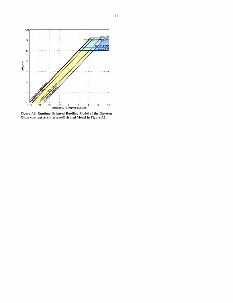
Figure A5 shows the traditional architectural-oriented model of the Opteron X4, while Figure A6 shows the runtime-oriented Roofline model for the Opteron X4 for a hypothetical kernel.

Figure A5. Traditional Architecture-Oriented Roofline Model for the Opteron X4, as presented earlier in the paper.

14

Figure A6. Runtime-Oriented Roofline Model of the Opteron X4, in contrast Architecture-Oriented Model in Figure A5.