


Languages
Pages
Legal


Proc. R. Soc. A (2010) 466, 2495–2516doi:10.1098/rspa.2010.0215
Published online 30 June 2010
REVIEW
Micro-architectured materials: past, presentand future
BY N. A. FLECK*, V. S. DESHPANDE AND M. F. ASHBY
Department of Engineering, University of Cambridge, Trumpington Street,Cambridge, CB2 1PZ, UK
Micro-architectured materials offer the opportunity of obtaining unique combinations ofmaterial properties. First, a historical perspective is given to the expansion of materialproperty space by the introduction of new alloys and new microstructures. Principlesof design of micro-architecture are then given and the role of nodal connectivity isemphasized for monoscale and multi-scale microstructures. The stiffness, strength anddamage tolerance of lattice materials are reviewed and compared with those of fully densesolids. It is demonstrated that micro-architectured materials are able to occupy regionsof material property space (such as high stiffness, strength and fracture toughness atlow density) that were hitherto empty. Some challenges for the development of futurematerials are highlighted.
Keywords: lattice materials; foams; mechanical properties
1. Introduction: a materials time-line
In this paper, the evolution of engineering materials is outlined with the mainenablers of change. The history of this evolution is illustrated in the firsttwo sections of the paper, introducing the concept of material property space.Strategies are identified for filling the remaining gaps of this space. The ability ofmicro-architectured lattice materials to give a wide range of stiffness, strength andfracture toughness is described, with the role of nodal connectivity and structuralhierarchy emphasized. The damage tolerance of lattice materials relative to thatof the parent solid is then discussed with an identification of several transition flawsizes. Finally, some future directions are given for the future development of latticematerials, and the utility of cross-property relations and bounding theorems isdiscussed.
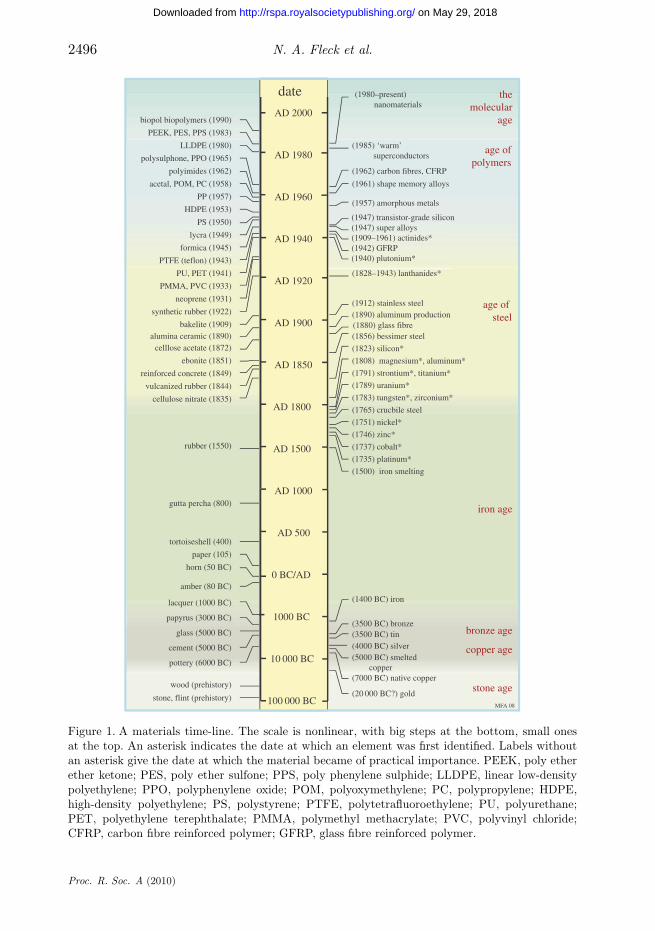
Figure 1 is a materials time-line. It is interesting to follow its development,starting from the bottom and working upwards. The tools and weapons ofprehistory, 300 000 or more years ago, were bone and stone. Stones could be
*Author for correspondence ([email protected]).
One contribution to the 2010 Anniversary Series ‘A collection of reviews celebrating the RoyalSociety’s 350th Anniversary’.
Received 22 April 2010Accepted 28 May 2010 This journal is © 2010 The Royal Society2495
on May 29, 2018http://rspa.royalsocietypublishing.org/Downloaded from
2496 N. A. Fleck et al.
date
100 000 BC
10 000 BC
1000 BC
0 BC/AD
AD 1000
AD 500
AD 1500
AD 1800
AD 1900
AD 1850
AD 1920
AD 1940
AD 1960
AD 1980
AD 2000biopol biopolymers (1990)
PEEK, PES, PPS (1983)
LLDPE (1980)
polysulphone, PPO (1965)
polyimides (1962)
acetal, POM, PC (1958)
PP (1957)
HDPE (1953)
PMMA, PVC (1933)
PS (1950)
lycra (1949)
formica (1945)
PTFE (teflon) (1943)
PU, PET (1941)
neoprene (1931)
lacquer (1000 BC)
horn (50 BC)
amber (80 BC)
tortoiseshell (400)
gutta percha (800)
rubber (1550)
cellulose nitrate (1835)
vulcanized rubber (1844)
ebonite (1851)
celllose acetate (1872)
bakelite (1909)
synthetic rubber (1922)
stone, flint (prehistory)
glass (5000 BC)
(20 000 BC?) gold
(5000 BC) smelted copper
(1400 BC) iron
(4000 BC) silver
stone age
copper age
bronze age
iron age
age of steel
age ofpolymers
(1735) platinum*
(1751) nickel*
(1737) cobalt*
(1746) zinc*
(1789) uranium*
(1940) plutonium*
(1783) tungsten*, zirconium*
(1791) strontium*, titanium*
(1808) magnesium*, aluminum*
(1823) silicon*
(1909–1961) actinides*
(1957) amorphous metals
(1828–1943) lanthanides*
(1961) shape memory alloys
(1500) iron smelting
(1856) bessimer steel
(1890) aluminum production
themolecular
age
(1947) super alloys
(1912) stainless steel
(1765) crucbile steel
cement (5000 BC)
(1980–present) nanomaterials
(1985) ‘warm’ superconductors
(7000 BC) native copper
MFA 08
reinforced concrete (1849)
(3500 BC) bronze(3500 BC) tin
wood (prehistory)
papyrus (3000 BC)
paper (105)
(1962) carbon fibres, CFRP
(1947) transistor-grade silicon
(1880) glass fibre
(1942) GFRP
alumina ceramic (1890)
pottery (6000 BC)
Figure 1. A materials time-line. The scale is nonlinear, with big steps at the bottom, small onesat the top. An asterisk indicates the date at which an element was first identified. Labels withoutan asterisk give the date at which the material became of practical importance. PEEK, poly etherether ketone; PES, poly ether sulfone; PPS, poly phenylene sulphide; LLDPE, linear low-densitypolyethylene; PPO, polyphenylene oxide; POM, polyoxymethylene; PC, polypropylene; HDPE,high-density polyethylene; PS, polystyrene; PTFE, polytetrafluoroethylene; PU, polyurethane;PET, polyethylene terephthalate; PMMA, polymethyl methacrylate; PVC, polyvinyl chloride;CFRP, carbon fibre reinforced polymer; GFRP, glass fibre reinforced polymer.
Proc. R. Soc. A (2010)
on May 29, 2018http://rspa.royalsocietypublishing.org/Downloaded from

Review. Micro-architectured materials 2497
shaped for tools, particularly flint and quartz, which can be flaked to producea cutting edge that was harder, sharper more durable than any other materialthat could be found in nature. Gold, silver and copper, the only metals thatoccur in native form, must have been known from the earliest time, but therealization that they were ductile, could be beaten to complex shape, and—oncebeaten—became hard, seems to have occurred around 5500 BC. By 4000 BC,there is evidence that the technology to melt and cast these metals had developed,allowing more intricate shapes. Native copper, however, is not abundant. Copperoccurs in far greater quantities as the minerals azurite and malachite. By 3500BC, kiln furnaces, developed for pottery, could reach the temperature requiredfor the reduction of these minerals, making copper sufficiently plentiful to be usedfor implements and weapons. But even in the worked state, copper is relativelysoft. Around 3000 BC, the accidental inclusion of a tin-based mineral, cassiterite,in the copper ores provided the next step in technology—the production of thealloy bronze, a mixture of tin and copper, with a strength and hardness that purecopper cannot match.
The discovery, around 1450 BC, of ways to reduce ferrous oxides to makeiron, a material with greater stiffness, strength and hardness than any other thenavailable, rendered bronze obsolete. Iron was not entirely new: tiny quantitiesexisted as the cores of meteors that had impacted the Earth. By contrast, theoxides of iron are widely available, particularly hematite, Fe2O3. Hematite is easilyreduced by carbon, although it takes high temperatures, close to 1100◦C, to doit. This temperature is insufficient to melt iron, so the material produced was aspongy mass of solid iron intermixed with slag; this was reheated and hammeredto expel the slag and then forged into the desired shape. The casting of ironwas a more difficult challenge, requiring temperatures of around 1600◦C. Twomillennia passed before, in AD 1500, the blast furnace was developed, enablingthe widespread use of cast iron. Cast iron allowed structures of a new type: thegreat bridges, railway terminals and civil buildings of the early nineteenth centuryare testimony to it. But it was steel, made possible in industrial quantities by theBessemer process of 1856, that gave iron its dominant role in structural designthat it still holds today.
The demands of the expanding aircraft industry in the 1950s shifted emphasisto the light alloys (those of aluminium, magnesium and titanium) and to materialsthat could withstand the extreme temperatures of the turbine combustionchamber. The development of superalloys—heavily alloyed iron, nickel and cobalt-based materials—became the focus of research, delivering an extraordinaryrange of alloys able to carry load at temperatures above 1200◦C. The range oftheir applications expanded into other fields, particularly those of chemical andpetroleum engineering.
The history of polymers is rather different. Wood, of course, is a polymericcomposite, one used for construction from the earliest times. The beauty ofamber—petrified resin—and of horn and tortoise shell—the polymer keratin—already attracted designers from the earliest times. Rubber, brought to Europein 1550, grew in importance in the nineteenth century, partly because ofthe wide spectrum of properties made possible by vulcanization—cross-linkingby sulphur—giving materials as elastic as latex or as rigid as ebonite. Thereal polymer revolution, however, has its beginnings in the early twentiethcentury with the development of Bakelite, a phenolic, in 1909 and synthetic
Proc. R. Soc. A (2010)
on May 29, 2018http://rspa.royalsocietypublishing.org/Downloaded from

2498 N. A. Fleck et al.
butyl rubber in 1922. This was followed, in mid-century, by a period ofrapid development of polymer science. Almost all the polymers we use sowidely today were developed in a 20 year span from 1940 to 1960, amongthem the bulk commodity polymers polypropylene, polyethylene, polyvinylchloride and polyurethane, the combined annual tonnage of which nowapproaches that of steel. Design with polymers has matured: they are now asimportant as metals in household products, automobiles and, most recently,in aerospace. Unreinforced polymers lack the stiffness and strength many ofthese applications demand. They are used, instead, as composites, reinforcedwith fillers and fibres. Composite technology is not new. Straw-reinforcedmud brick is one of the earliest of the materials of architecture and remainsone of the traditional materials for building in parts of Africa and Asia,even today. Steel-reinforced concrete—the material of shopping centres, roadbridges and apartment blocks—appeared just before 1850. The reinforcementof polymers was enabled by the technology for making glass fibres, whichhad existed since 1880. Glass wool, or better, woven or layered glass fibres,could be incorporated in thermosetting polyesters or epoxies, giving themthe stiffness and strength of aluminium alloys. By the mid-1940s, glass fibrereinforced polymer components were in use in the aircraft industry. The realtransformation of polymers into high-performance structural materials camewith the development of aramid and carbon fibres in the 1960s. Incorporatedas reinforcements, they give materials with performance (meaning stiffness andstrength per unit weight) which exceeded that of all other bulk materials,giving them their now-dominant position in high-performance sports equipmentand aerospace.
The period in which we now live might have been named the polymers andcomposites era had it not coincided with a second revolution that is based onsilicon. Silicon was first identified as an element in 1823, but found few uses untilthe discovery, in 1947, that, when doped with tiny levels of impurity, it couldact as a rectifier. The discovery has created the fields of electronics, mechatronicsand modern computer science, revolutionizing information storage, access andtransmission, imaging, sensing and actuation, numerical modelling and muchmore. This is rightly called the information age, enabled by the developmentof transistor-grade silicon.
In the last two decades, the area of biomaterials has developed rapidly.Implanting materials in or on the human body was not practical until the asepticsurgical technique was developed in the late 1800s. Non-toxic metal alloys wereintroduced, but tended to fracture in service. It was not until the developmentof polymer-based systems, and subsequently, with a new wave of discoveries incell biology, chemistry and materials science, that synthetic biomaterials becamea reality.
During the early 1990s, it was realized that material behaviour depended onscale, and that the dependence was most evident when the scale was that ofnanometres. Although the term nanoscience is new, the use of nanotechnologyis not. The proteins and minerals of soft and mineralized tissue in plants andanimals are dispersed on a nano-scale. Nanoparticles of carbon have been usedfor the reinforcement of tyres. The light alloys of aerospace derive their strengthfrom a nano-scale dispersion of precipitates. Modern nanotechnology gainedprominence with the discovery of various forms of carbon such as the C60
Proc. R. Soc. A (2010)
on May 29, 2018http://rspa.royalsocietypublishing.org/Downloaded from
Review. Micro-architectured materials 2499
molecule and carbon nanotubes, though even these are not really new but havealways existed as particles in smoke. True nano-engineering has finally comewith the development of tools capable of resolving and manipulating matterat the atomic level, making it possible (though at present expensive) to buildmaterials and structures the way nature does it, atom by atom and moleculeby molecule.
Figure 1 tracks the expanding portfolio of materials available to the engineer.With it comes an expansion of the accessible range of stiffness, strengthand toughness. The expansion of one of these—strength—is illustrated in thenext section.
2. Expanding the boundaries of material property space
The material development documented in the time-line were driven by the desirefor ever greater performance. One way of examining the progress of this is byfollowing the way in which properties have evolved on material property charts.Material property charts (Ashby 2010) display materials on axes based on two oftheir properties. Materials have many properties of course (mechanical, thermal,electrical, optical, etc.) and so the number of such pair-wise combinations is large.Each chart can be thought of as a slice through ‘material property space’—amulti-dimensional space with material properties as its axes.
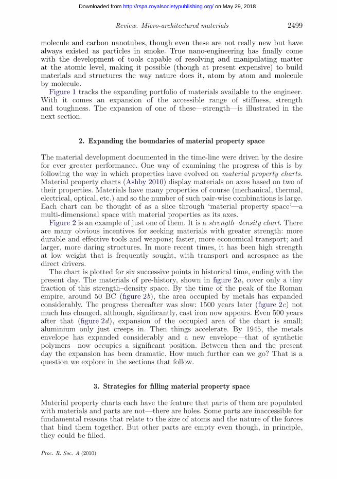
Figure 2 is an example of just one of them. It is a strength–density chart. Thereare many obvious incentives for seeking materials with greater strength: moredurable and effective tools and weapons; faster, more economical transport; andlarger, more daring structures. In more recent times, it has been high strengthat low weight that is frequently sought, with transport and aerospace as thedirect drivers.
The chart is plotted for six successive points in historical time, ending with thepresent day. The materials of pre-history, shown in figure 2a, cover only a tinyfraction of this strength–density space. By the time of the peak of the Romanempire, around 50 BC (figure 2b), the area occupied by metals has expandedconsiderably. The progress thereafter was slow: 1500 years later (figure 2c) notmuch has changed, although, significantly, cast iron now appears. Even 500 yearsafter that (figure 2d), expansion of the occupied area of the chart is small;aluminium only just creeps in. Then things accelerate. By 1945, the metalsenvelope has expanded considerably and a new envelope—that of syntheticpolymers—now occupies a significant position. Between then and the presentday the expansion has been dramatic. How much further can we go? That is aquestion we explore in the sections that follow.
3. Strategies for filling material property space
Material property charts each have the feature that parts of them are populatedwith materials and parts are not—there are holes. Some parts are inaccessible forfundamental reasons that relate to the size of atoms and the nature of the forcesthat bind them together. But other parts are empty even though, in principle,they could be filled.
Proc. R. Soc. A (2010)
on May 29, 2018http://rspa.royalsocietypublishing.org/Downloaded from
2500 N. A. Fleck et al.
oakpine
fir
balsa
ash
oak
pine
firbalsafoams
polymers and elastomers
metals
ceramics
composites
natural materials
lead alloys
W alloys
steelsTi alloys
Mg alloys
CFRP
GFRP
Al alloys
rigid polymer foams
flexible polymer foams
Ni alloys
Cu alloys
zinc alloys
PA PEEKPC PET
cork
butyl rubber
silicone elastomers
concrete
tungstencarbide
Al2O3
SiC
Si3N4
MFA, 09
osmium
gold
silver
diamond
Zr alloys
Pt alloys
Be alloys
density, ρ (kg m–3)10 10 000100 1000 100 000
0.01
0.1
1
10
102
103
104
105
metals ceramicsand glasses
naturalmaterials
lead
gold
silver
bronze
steels
concrete
brick
stone
pottery
ash woods, // to grain
cork
oakpine
fir
balsa
ash
oak
pine
firbalsa
tin
copper
cast ironsAl-alloys
Mg-alloys
titanium
zincrubber
woods, to grainT
PE
acrylic
bakeliteepoxy
polymers and elastomers
stre
ngth
, σf (
MPa
)
density, ρ (kg m–3)
10 10 000100 1000 100 000
metals ceramicsand glasses
naturalmaterials
lead
gold
silver
bronze
steels
glass
concrete
brick
stone
pottery
ash
woods, // to grain
cork
oakpine
fir
balsa
ashoak
pine
firbalsa
leather
bone
tin
copper
cast irons
aluminum
zinc
polymers
gg
rubber
woods, to grainT
0.01
0.1
1
10
102
103
104
105
metals ceramicsand glasses
naturalmaterials
lead
gold
silver
bronze
wrought iron
glass
concrete
brick
stone
pottery
ash woods, // to grain
cork
oakpine
fir
balsa
ash
oak
pine
firbalsa
leathershellbone
tin
copper
cast iron
woods, to grainT
stre
ngth
, σf (
MPa
)
metals ceramicsand glasses
naturalmaterials
lead
gold
silver
bronzewrought iron
glass
concrete
brick
stone
pottery
ash
woods, // to grain
cork
oakpine
fir
balsa
ash
oak
pine
firbalsa
leathershellbone
tin
copper
woods, to grainT
stre
ngth
, σf (
MPa
)
0.01
0.1
1
10
102
103
104
105prehistory: 50 000 BC 50 BC
AD 1900AD 1500
present dayAD 1945
metals ceramicsand glasses
naturalmaterials
gold
bone
stone
pottery
ash
woods, // to grain
oakpine
fir
balsa
ash
oak
pine
firbalsa
leather
(a) (b)
(c) (d)
(e) ( f )
antler
shell
woods, to grainT
Figure 2. The progressive filling of material property space over time (the charts list the dateat the top left)—here the way the materials have been developed over time to meet demandson strength and density. Similar time plots show the progressive filling of similar plots for allmaterial properties. PE, polyethylene; CFRP, carbon fibre reinforced polymer; GFRP, glass fibrereinforced polymer; PEEK, poly ether ether ketone; PA, polyamide; PC, polycarbonate; PET,polyethylene terephthalate.
Proc. R. Soc. A (2010)
on May 29, 2018http://rspa.royalsocietypublishing.org/Downloaded from

Review. Micro-architectured materials 2501
One approach to filling holes in material property space is that of manipulatingchemistry, developing new metal alloys, new polymer formulations and newcompositions of glass and ceramic, which extends the populated areas of theproperty charts. A second is that of manipulating microstructure, using thermo-mechanical processing to control the distribution of phases and defects withinmaterials. Both have been exploited systematically, leaving little room for furthergains, which tend to be incremental rather than step like. A third approachis that of controlling architecture to create hybrid materials—combinations ofmaterials or of material and space in configurations and with connectivities thatoffer enhanced performance. The success of carbon and glass-fibre reinforcedcomposites at one extreme, and of foamed materials at another, in fillingpreviously empty areas of the property charts is encouragement enough to explorethis route in greater depth. In the present study, we limit attention to the extremecase of porous solids (a hybrid of the solid and air), and explore the effect ofmicro-architecture upon properties.
(a) Lattice materials
We define a general lattice material as a cellular, reticulated, truss or latticestructure made up of a large number of uniform lattice elements (e.g. slenderbeams or rods) and generated by tessellating a unit cell, comprised of justa few lattice elements, throughout space. Here, we use the term ‘material’ toemphasize that we shall consider lattices with global, macroscopic length scalesmuch larger than that characteristic of their constituent lattice elements (e.g.individual rod length). For the lattice to behave as a material, the wavelengthof any loading is also much longer than that of the lattice elements. In contrast,the lattice behaves as a ‘structure’ when it contains a relatively small number oflattice elements, and the length scale of the loading is comparable to that of thelattice elements.
Classically, periodic planar lattices are classified as regular, semi-regularor other. Regular lattices are generated by tessellating a regular polygon tofill the entire plane (Cundy & Rolett 1961; Lockwood & Macmillan 1978;Frederickson 1997). Only a few regular polygons produce such a lattice: theseare the triangle, square and hexagon, with sketches of the triangulated andhexagonal lattice included in figure 3. Semi-regular lattices are generated bytessellating two or more different kinds of regular polygons to fill the entireplane (Cundy & Rolett 1961; Lockwood & Macmillan 1978; Frederickson 1997).It may be shown that there exist only eight, independent, such lattices and nomore. An example of such a lattice is the ‘triangular–hexagonal’ lattice, alsoknown as the Kagome lattice (Syozi 1972; Hyun & Torquato 2002). Additionalplane-filling lattices can be constructed from two or more polygons of differentsize, or by relaxing the restriction that each joint has the same connectivity(e. g. Hutchinson 2004).
Spatial or three-dimensional lattices can be generated by filling space frompolyhedra. Of the regular polyhedra with a small number of faces, only the cubeand the rhombic dodecahedra can be tessellated to fill all space (Gibson & Ashby1997). Typically, spatial lattices are constructed using combinations of differentpolyhedra, for example, tetrahedra and octahedra may be packed to form theoctet-truss lattice (Deshpande et al. 2001a).
Proc. R. Soc. A (2010)
on May 29, 2018http://rspa.royalsocietypublishing.org/Downloaded from

2502 N. A. Fleck et al.
(a) (b)
(c)
x1
x2
x1
x2
x1
x2
Figure 3. (a) Kagome lattice, (b) triangular lattice and (c) hexagonal lattice.
In the following, we shall argue that the properties of lattice materials aredictated by the volume fraction of cell-wall material and also by the nodalconnectivity: the number of struts that meet at each node of the microstructure.
4. Expanding property space by the design of lattice materials
The relative density r̄ of a lattice material is defined as the ratio of the densityof the lattice material to the density of the solid. Lattice materials resembleframeworks when r̄ is less than about 0.2, and in this regime r̄ is directly relatedto the thickness t and length � of a strut according to
r̄ = A(
t�
)(4.1)
for a two-dimensional lattice. The constant of proportionality A depends uponthe geometry: for the hexagonal, Kagome and fully triangulated lattices as shownin figure 3, we find that A equals 2/
√3,
√3 and 2
√3, respectively, as listed
in table 1.
Proc. R. Soc. A (2010)
on May 29, 2018http://rspa.royalsocietypublishing.org/Downloaded from

Review. Micro-architectured materials 2503
Table 1. Coefficients for the scaling laws.
topology A B b v C c D d
hexagonal 2/√
3 3/2 3 1 1/3 2 0.90 2triangular 2
√3 1/3 1 1/3 1/3 1 0.61 1
Kagome√
3 1/3 1 1/3 1/2 1 0.21 1/2
A three-dimensional lattice or foam can be either open or closed celled asfollows. Open-cell microstructures comprise a three-dimensional arrangement ofinter-connected struts, and have the property that r̄ scales with (t/�)2. Closed-cell microstructures also exist, with plate-like cell faces of thickness t and sidelength �; their relative density scales with (t/�), provided the cell faces haveuniform thickness. Closed-cell foams, typically, have thickened cell edges; givinga dependence of r̄ on (t/�) between these two extremes.
(a) The role of nodal connectivity
There are two distinct species of cellular solid. The distinction is most obviousin their mechanical properties. The first, typified by foams, are bending-dominatedstructures; the second, typified by triangulated lattice structures, are stretching-dominated structures—a distinction explained more fully below, and detailed inDeshpande et al. (2001b). To give an idea of the difference: a foam with a relativedensity of 0.1 (meaning that the solid cell walls occupy 10% of the volume) is lessstiff by a factor of 3 than a triangulated lattice of the same relative density. Themacroscopic properties are largely dictated by the connectivity of joints ratherthan by the regularity of the microstructure.
The distinction of a bending-dominated structure and a stretching-dominatedmicrostructure structure is closely linked to the collapse response of a pin-jointedstructure of the same morphology. If the parent pin-jointed lattice exhibitscollapse mechanisms that generate macroscopic strain, then the welded-jointversion relies upon the rotational stiffness and strength of the nodes and struts forits macroscopic behaviour: consequently, the parent lattice is bending dominated.In contrast, when the parent lattice has only periodic collapse mechanisms or nocollapse mechanisms, the welded-joint version is stretching governed. In broadterms, the type of response is dependent upon the nodal connectivity.
Maxwell analysed a pin-jointed frame (meaning one that is hinged at itscorners) made up of b struts and j frictionless joints, like those in figure 3. Heshowed that a two-dimensional statically and kinematically determinate frame(one that is just rigid and does not fold up when loaded) has the property that
b − 2j + 3 = 0. (4.2)
In a three-dimensional frame, the equivalent equation is
b − 3j + 6 = 0. (4.3)
A generalization of the Maxwell rule in three-dimensional space is given byCalladine (1978) as follows:
b − 3j + 6 = s − m, (4.4)
Proc. R. Soc. A (2010)
on May 29, 2018http://rspa.royalsocietypublishing.org/Downloaded from
2504 N. A. Fleck et al.
Kagome
squaretriangular–triangular
triangular
strain-producingmechanisms no mechanisms
hexagonal
periodicmechanisms
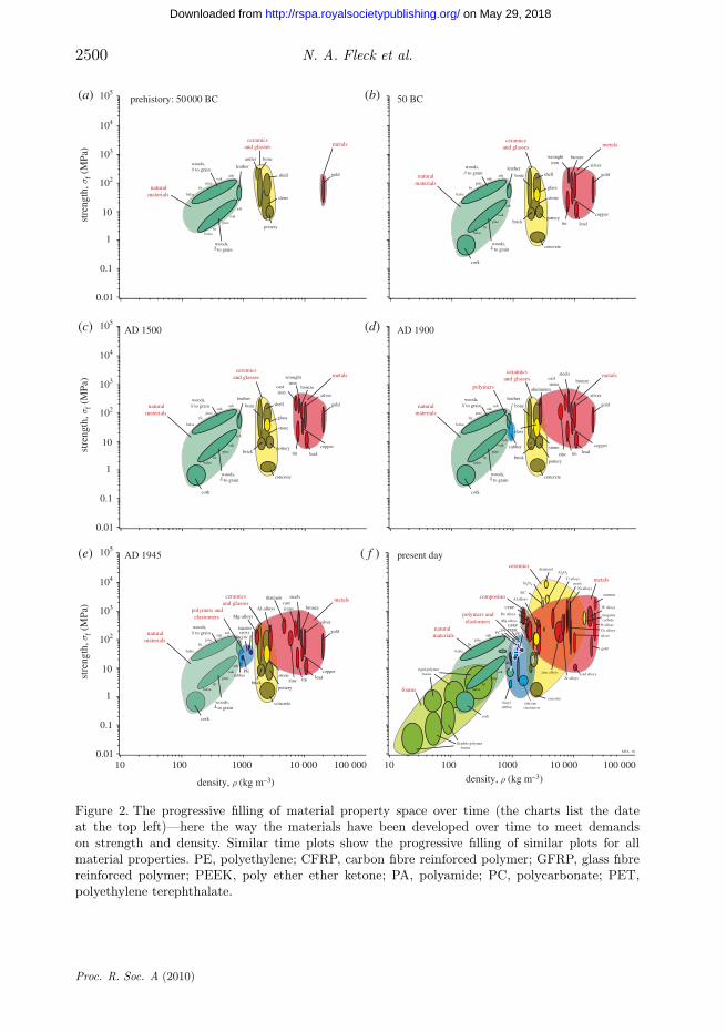
Figure 4. Venn diagram for selected two-dimensional lattices.
where s and m count the states of self-stress and mechanisms, respectively, andeach can be determined by finding the rank of the equilibrium matrix thatdescribes the frame in a full structural analysis (Pellegrino & Calladine 1986).A just rigid framework (i.e. a framework that is both statically and kinematicallydeterminate) has s = m = 0. The nature of Maxwell’s rule as a necessary ratherthan sufficient condition is made clear by examination of equation (4.2): vanishingof the LHS in equation (4.2) only implies that the number of mechanisms andstates of self-stress are equal, not that each equals zero. If m > 0, then the framecontains mechanisms. It has no stiffness or strength; it collapses if loaded. If itsjoints are locked, preventing rotation (as they are in a lattice), the bars of theframe bend. If, instead, m = 0, then the frame ceases to be a mechanism. If itis loaded, its members carry tension or compression (even when pin jointed),and it becomes a stretch-dominated structure. Locking the hinges now makeslittle difference because slender structures are much stiffer when stretched thanwhen bent.
We now turn our attention to a large pin-jointed framework of connectivity Zand j joints: the total number of bars b is approximately jZ/2. The necessary,but not sufficient, condition for rigidity is Z = 4 in two-dimensional space andZ = 6 in three-dimensional space (Deshpande et al. 2001b). A Venn diagram toillustrate the various types of mechanism exhibited by classes of a two-dimensionalperiodic pin-jointed truss is given in figure 4. Consider the various structuresin turn. The fully triangulated structure, comprising equilateral triangles witha nodal connectivity of Z = 6, is highly redundant and possesses no collapsemechanisms. In contrast, a triangular–triangular lattice, with unit cell shownin figure 4, collapses by a mechanism that leads to a macroscopic hydrostaticstrain. Thus, this structure has zero macroscopic stiffness against this collapsemode. The Kagome microstructure has a connectivity of Z = 4 and has no strain-producing collapse mechanisms; it can only collapse by periodic mechanisms thatdo not produce a macroscopic strain. Consequently, it is rigid in all directions.The cases of the square lattice and the hexagonal lattice, with a connectivityof Z = 4 and Z = 3, respectively, are different. Each of these structures cancollapse by macroscopic strain-producing mechanisms, and by periodic collapse
Proc. R. Soc. A (2010)
on May 29, 2018http://rspa.royalsocietypublishing.org/Downloaded from

Review. Micro-architectured materials 2505
mechanisms. A methodology has been developed by Hutchinson & Fleck (2005)to explore the periodic collapse mechanisms based on Bloch-wave analysis; thedetails are beyond the scope of the present article. The main conclusion todraw from figure 4 is that the fully triangulated structure is macroscopicallystiff because it possesses no collapse mechanisms, while the Kagome structureis macroscopically stiff because it has only periodic collapse mechanisms thatgenerate no macroscopic strain.
(b) The in-plane stiffness of two-dimensional isotropic lattice materials
Material property space can be expanded by suitable design of materialarchitecture. To illustrate this, consider the in-plane properties of two-dimensional isotropic lattice materials: the hexagonal, Kagome and triangularlattices of nodal connectivity 3, 4 and 6, respectively, as sketched in figure 3.We begin by reviewing briefly the macroscopic in-plane stiffness of these two-dimensional lattices. Simple beam theory can be used to determine the effective,macroscopic Young modulus E and Poisson ratio n of the lattices in terms of therelative density r̄ and the Young modulus of the solid ES. The scaling law can beadequately represented by the power-law expression
EES
= Br̄b, (4.5)
where the values of the coefficient B and exponent b are listed in table 1. ThePoisson ratio n is independent of relative density, assuming it is sufficiently lowfor beam theory to be adequate in characterizing the behaviour of the latticematerial. But n does depend upon geometry, as summarized in table 1. Thehexagonal lattice is bending dominated, with b = 3. In contrast, the Kagomeand fully triangulated lattices are stretching dominated, with b = 1. Remarkably,the coefficient B and the Poisson ratio are also identical for the triangulatedand Kagome lattices: these lattices have identical effective properties, and eachachieves the Hashin–Shtrikhman upper bound. The differences between the twolattices do show up however when imperfections are introduced. For example, byrandomly perturbing the location of the nodes at fixed relative density, there is alarge drop in the modulus of the Kagome lattice, but a much smaller drop in themodulus of the triangulated lattice (Romijn & Fleck 2007). This is due to the factthat the triangulated lattice has a higher nodal connectivity of Z = 6 than thatof the Kagome lattice (Z = 4) and is a much more redundant structure when thestruts are assumed to be pin jointed at the nodes. The role of imperfection forthese two lattices is further explored below for the property of fracture toughness.
(c) The strength of two-dimensional lattice materials
Beam theory can also be used to determine the macroscopic fracture strengthof the perfect lattice, in the absence of heterogeneities such as a macroscopiccrack. Consider the lattices of figure 3 loaded macroscopically by a uniform in-plane stress. The lattice responds in a linear-elastic manner, with a stress statewithin each bar given by simple beam theory. Define failure of the lattice as thepoint at which the maximum local tensile stress within the lattice attains thetensile fracture strength of the solid sTS. The corresponding macroscopic stressdefines the fracture strength of the lattice. None of the three lattices of figure 3
Proc. R. Soc. A (2010)
on May 29, 2018http://rspa.royalsocietypublishing.org/Downloaded from

2506 N. A. Fleck et al.
possess an isotropic fracture strength—the macroscopic tensile strength of thelattice varies with the direction of loading. However, Gibson & Ashby (1997)have shown that the degree of anisotropy is small. For definiteness, we reviewhere the macroscopic uniaxial strength sc of the lattice, upon loading along thex2 direction as shown in figure 3. The strength sc can be expressed in terms ofthe tensile fracture strength of the solid sTS as follows:
sc
sTS= C r̄c, (4.6)
with the coefficients (C , c) dependent upon geometry, as listed in table 1. Thetriangular and Kagome structures deform by bar stretching, and this leads toc = 1, while the hexagonal honeycomb deforms by bar bending, giving c = 2.
(d) Three-dimensional lattices and foams
Now consider the case of open-cell metallic foams, as reviewed by Ashby et al.(2000). They are manufactured mostly from the melt by the expansion of gasbubbles, and the expansion process is driven by the minimization of surfaceenergy. Consequently, they have microstructures that, although stochastic, have alow nodal connectivity of 3–4 adjoining bars per joint. The stiffness and strengthof these three-dimensional structures relies upon the bending stiffness of the bars,and they are consequently referred to as bending-dominated structures. It followsfrom beam-bending theory and dimensional analysis that the Young modulusE of open-cell foams scales with that of the fully dense solid ES according toE ≈ r̄2ES. The yield strength sY scales with r̄ and with the yield strength ofthe parent solid sYS according to sY ≈ 0.3r̄3/2sYS. Both relations are supportedby a wealth of experimental data (see Ashby et al. 2000). In contrast, the octettruss, identical in crystal structure to face-centred cubic, has a nodal connectivity(coordination number) of 12 and is a stretching-dominated structure. Stretching-dominated microstructures have the property that their Young modulus E andtheir yield strength sY scale linearly with relative density r̄, such that E ≈ 0.3r̄ESand sY ≈ 0.3r̄sYS. (These values are of the order of the Hashin–Shtrikhman upperbound for an isotropic solid.) Such lattice materials have the virtue that thestiffness and strength scale linearly with the relative density and thereby out-perform metallic foams. A variety of fabrication routes have evolved to constructthese periodic lattices (see Wadley et al. 2003).
It is instructive to display bending-dominated foams and stretching-dominatedlattice materials in property space using the axes of E versus density and sYversus density (see figure 5). The properties of the lattice materials scale linearlywith density from that of the parent material, and fill-in some of the gaps ofmaterial property space. In contrast, the stiffness and strength of foams degradeat a faster rate than linearly with a decrease in density.
5. Multi-scale lattice materials
Nature makes use of multi-scale lattice materials, such that the material withineach strut of the lattice comprises a lattice on a successively smaller scale (Ashby1991, 2010). One reason for such structural hierarchy in engineering structures
Proc. R. Soc. A (2010)
on May 29, 2018http://rspa.royalsocietypublishing.org/Downloaded from

Review. Micro-architectured materials 2507
is to increase buckling strength: recall that the buckling strength scales with anyrepresentative strut length � according to �−2, and so the finer the length scale,the higher the buckling strength.
Nature frequently designs compliant structures that have sufficiently lowmoduli that low stresses are generated upon deformation, and the structuresdo not fail. Soft tissue is of this type: skin, cartilage and elastin, along with manytypes of bird’s nests such as the woven Weaver bird’s nest. One way of achievinglow stiffness is to use structural hierarchy with a bending-dominated structureon various length scales.
Consider as a prototypical example a lattice material with struts (labelled 1)on a large scale made in turn from another lattice material with struts on afine scale (labelled 2), as sketched in figure 6. The effective modulus E2 of thefine-scale struts scales with the modulus ES and relative density of the fine-scalestruts r̄2 according to
E2 = B2r̄b22 ES. (5.1)
Now construct the larger scale lattice material such that its struts are made fromthe fine-scale lattice of modulus E2. With the volume fraction of strut material 2in the lattice material 1 written as r̄1, we note that the relative density of latticematerial 1 to the solid is r̄ = r̄1r̄2. Also, the effective modulus of the coarse-scalelattice E1 is
E1 = B1r̄b11 E2 = B1B2r̄
b11 r̄
b22 ES, (5.2)
and for the case b1 = b2, this simplifies to
E1 = B1B2r̄b1ES. (5.3)
Now consider some examples from nature where the large-scale lattice 1 is abending or stretching structure and the finer-scale lattice 2 (making up the strutsof the larger lattice) is a bending or stretching structure. We consider each casein turn.
(a) Case I: a stretching–stretching structure
When both lattices have sufficient nodal connectivity that they are stretching-dominated in behaviour, we have b1 = b2 = 1 and the overall modulus E1 is high.An example of this is the axial stiffness of woods: the cell walls are arranged ashexagonal prisms and, along the prismatic direction, the macro-lattice undergoesplate stretching. On a finer scale, each cell wall contains long fibres of celluloseand these too undergo stretching.
(b) Case II: a bending–bending structure
Highly compliant lattices can be made by exploiting bending of the primarystruts of the lattice, along with the use of compliant cell-wall material (bending-dominated deformation of the finer-scale lattice). For an open-cell foam-likestructure on both lengths scales, we have b1 = b2 = 2. Consider as an example,birds nests that have been made by weaving together the leaves of grass. Thegrass leaves are wavy and bend when the nest is deformed. And on a finer-scale
Proc. R. Soc. A (2010)
on May 29, 2018http://rspa.royalsocietypublishing.org/Downloaded from

2508 N. A. Fleck et al.
E1/3
ρ
E1/2
ρEρ
guide lines for minimum mass
design
You
ng’s
mod
ulus
, E (
GPa
)
10–4
10–3
10–2
10–1
1
10
100
1000
(a)
(b)
polyester
foams
polymers
metals
technicalceramics
composites
natural materials
lead alloys
W alloys
steels
Ti alloys
Mg alloys
CFRP
GFRP
Al alloys
flexible polymer foams
Ni alloys
Cu alloys
zinc alloysPAPEEK
PMMA
PC
PET
cork
wood
butyl rubber
silicone elastomers
concrete
WC
Al2O3SiC
Si3N4B4C
epoxiesPS
PTFE
EVA
neopreneisoprene
polyurethane
leather
MFA, 2010
PP
PE
glass
// grain
grainT
elastomers
wood
non-technicalceramics
bamboo
PAA
sP
PAA
oysFRP
PMMMAMA
in
ysP
ysP
loysFRP
PMMAM
in
ysP
polyesp yester
PS
graiTwood
esster
PS
graiTwo
lyes
CFRP lattice
CFRP foam
aluminium lattice
aluminium foam
σf1/2
ρ
σf2/3
ρ
σfρ
density, ρ (kg m3)
10 100 1000 10 000
MFA, 2010
guide lines for minimum mass
design
stre
ngth
, σf (
MPa
)
0.01
0.1
1
10
100
1000
10 000
PPPE
woods,
T
foams
polymers and elastomers
metalsceramics
composites
natural materials
lead alloys
tungsten alloys
steelsTi alloys
Mg alloys
CFRP
GFRP
Al alloys
flexible polymer foams
Ni alloys
copper alloys
zinc alloys
PA PEEK
PMMAPC
PET
cork
woods, ll
butyl rubber
silicone elastomers
concrete
tungstencarbide
Al2O3SiC
Si3N4
metals and polymers: yield strength, σyceramics, glasses: modulus of rupture, MORelastomers: tensile tear strength, σtcomposites: tensile failure, σt
PA
MMAPC
, ll
PPA
MMAPC
s, llA
PE
CFRP lattice
CFRP foam
aluminium lattice
PA
PMMPC
woods
APA
PMMPC
woods
APA
TPEE
PP
TTTTET
PP
TTTET
aluminium foam
Figure 5. Material property charts of (a) E versus r and (b) sY versus r for engineeringmaterials. Predictions for bending-dominated foams and stretching-dominated lattices of CFRPand aluminium are superimposed. Lattices expand the occupied area of both charts. PMMA,polymethyl methacrylate; PA, polyamide; PEEK, poly ether ether ketone; PS, polystyrene; PP,polypropylene; PET, polyethylene terephthalate; PE, polyethylene; PC, polycarbonate; PTFE,polytetrafluoroethylene; CFRP, carbon fibre reinforced polymer; EVA, ethylene vinyl acetate.
Proc. R. Soc. A (2010)
on May 29, 2018http://rspa.royalsocietypublishing.org/Downloaded from
Review. Micro-architectured materials 2509
coarse scale lattice
fine-scalelattice
1 2
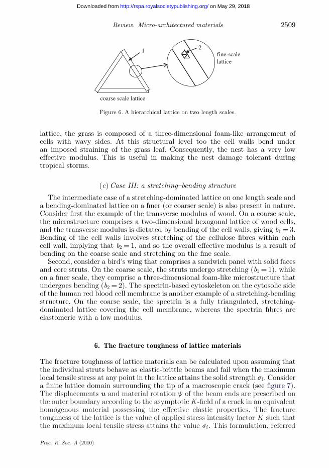
Figure 6. A hierarchical lattice on two length scales.
lattice, the grass is composed of a three-dimensional foam-like arrangement ofcells with wavy sides. At this structural level too the cell walls bend underan imposed straining of the grass leaf. Consequently, the nest has a very loweffective modulus. This is useful in making the nest damage tolerant duringtropical storms.
(c) Case III: a stretching–bending structure
The intermediate case of a stretching-dominated lattice on one length scale anda bending-dominated lattice on a finer (or coarser scale) is also present in nature.Consider first the example of the transverse modulus of wood. On a coarse scale,the microstructure comprises a two-dimensional hexagonal lattice of wood cells,and the transverse modulus is dictated by bending of the cell walls, giving b1 = 3.Bending of the cell walls involves stretching of the cellulose fibres within eachcell wall, implying that b2 = 1, and so the overall effective modulus is a result ofbending on the coarse scale and stretching on the fine scale.
Second, consider a bird’s wing that comprises a sandwich panel with solid facesand core struts. On the coarse scale, the struts undergo stretching (b1 = 1), whileon a finer scale, they comprise a three-dimensional foam-like microstructure thatundergoes bending (b2 = 2). The spectrin-based cytoskeleton on the cytosolic sideof the human red blood cell membrane is another example of a stretching-bendingstructure. On the coarse scale, the spectrin is a fully triangulated, stretching-dominated lattice covering the cell membrane, whereas the spectrin fibres areelastomeric with a low modulus.
6. The fracture toughness of lattice materials
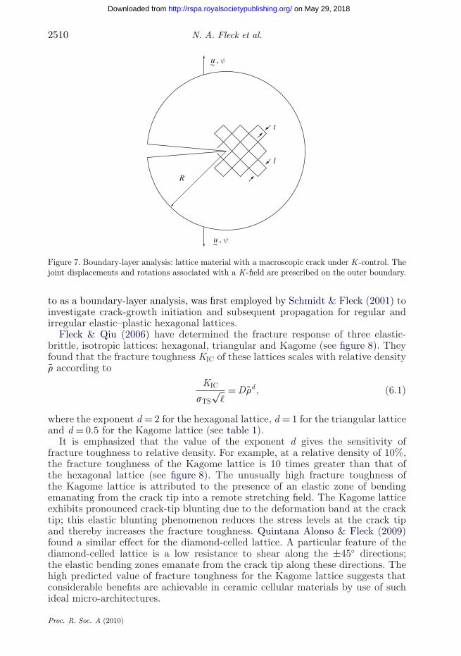
The fracture toughness of lattice materials can be calculated upon assuming thatthe individual struts behave as elastic-brittle beams and fail when the maximumlocal tensile stress at any point in the lattice attains the solid strength sf . Considera finite lattice domain surrounding the tip of a macroscopic crack (see figure 7).The displacements u and material rotation j of the beam ends are prescribed onthe outer boundary according to the asymptotic K -field of a crack in an equivalenthomogenous material possessing the effective elastic properties. The fracturetoughness of the lattice is the value of applied stress intensity factor K such thatthe maximum local tensile stress attains the value sf . This formulation, referred
Proc. R. Soc. A (2010)
on May 29, 2018http://rspa.royalsocietypublishing.org/Downloaded from
2510 N. A. Fleck et al.
l
t
R
, u ψ~
, u ψ~
Figure 7. Boundary-layer analysis: lattice material with a macroscopic crack under K -control. Thejoint displacements and rotations associated with a K -field are prescribed on the outer boundary.
to as a boundary-layer analysis, was first employed by Schmidt & Fleck (2001) toinvestigate crack-growth initiation and subsequent propagation for regular andirregular elastic–plastic hexagonal lattices.
Fleck & Qiu (2006) have determined the fracture response of three elastic-brittle, isotropic lattices: hexagonal, triangular and Kagome (see figure 8). Theyfound that the fracture toughness KIC of these lattices scales with relative densityr̄ according to
KIC
sTS√
�= Dr̄d , (6.1)
where the exponent d = 2 for the hexagonal lattice, d = 1 for the triangular latticeand d = 0.5 for the Kagome lattice (see table 1).
It is emphasized that the value of the exponent d gives the sensitivity offracture toughness to relative density. For example, at a relative density of 10%,the fracture toughness of the Kagome lattice is 10 times greater than that ofthe hexagonal lattice (see figure 8). The unusually high fracture toughness ofthe Kagome lattice is attributed to the presence of an elastic zone of bendingemanating from the crack tip into a remote stretching field. The Kagome latticeexhibits pronounced crack-tip blunting due to the deformation band at the cracktip; this elastic blunting phenomenon reduces the stress levels at the crack tipand thereby increases the fracture toughness. Quintana Alonso & Fleck (2009)found a similar effect for the diamond-celled lattice. A particular feature of thediamond-celled lattice is a low resistance to shear along the ±45◦ directions;the elastic bending zones emanate from the crack tip along these directions. Thehigh predicted value of fracture toughness for the Kagome lattice suggests thatconsiderable benefits are achievable in ceramic cellular materials by use of suchideal micro-architectures.
Proc. R. Soc. A (2010)
on May 29, 2018http://rspa.royalsocietypublishing.org/Downloaded from

Review. Micro-architectured materials 2511
100
10–1
10–2
0.51
KIC
/σT
S√l 1
1
1
210–3
10–4
10–5
10–6
10–7
10–3 10–2 10–1
relative density, ρ
Figure 8. The predicted mode I fracture toughness KIC plotted as a function of relative densityr̄ ∝ t/�, for the three isotropic lattices: hexagonal, triangular and Kagome.
We proceed to relate the fracture toughness KIC of a lattice to the fracturetoughness K S
IC of the cell-wall material. Assume that the fracture strength sTS ofthe cell wall of a lattice material is dictated by the fracture toughness of the cellwall K S
IC via an intrinsic flaw size a0, according to
sTS = K SIC√
pa0. (6.2)
Now substitute into (6.1) to obtain
KIC
K SIC
= Dr̄d(
�
pa0
)1/2
. (6.3)
This expression is valid at low relative density. At high relative density, a moreaccurate expression would be
KIC
K SIC
= r̄. (6.4)
To obtain a single expression that attains both asymptotes, we introduce anarbitrary weight function w(r̄), where
w(r̄) = exp(
− r̄
(1 − r̄)r̄0
). (6.5)
Proc. R. Soc. A (2010)
on May 29, 2018http://rspa.royalsocietypublishing.org/Downloaded from

2512 N. A. Fleck et al.
10−2 10−1 1000
0.2
0.4
0.6
0.8
1.0
ρ
KIC
/K s IC
l/a0 = 1000
l/a0 = 100
l/a0 = 10
Figure 9. Predictions of the scaling of the fracture toughness of the Kagome lattice with relativedensity for three choices of the length scale ratio �/a0 and r̄0 = 0.3.
The parameter r̄0 can be interpreted to be the value of relative density at whichthe fracture toughness switches from the dilute lattice limit to that of a solidcontaining a dilute concentration of voids. Upon combining (6.3–6.5), we obtain
KIC
K SIC
= w(r̄)Dr̄d(
�
pa0
)1/2
+ (1 − w(r̄))r̄. (6.6)
The weight function has the required asymptotic limits of w(0) = 1 and w(1) = 0in order for (6.6) to reduce to (6.3) and to (6.4) when r̄ equals 0 and 1, respectively.The relation (6.6) is plotted in figure 9 for three representative choices of theratio �/a0 and the transition relative density r̄0 = 0.3. For high values of �/a0,the fracture toughness of the lattice can be comparable to that of the parentsolid material, even though the effective density of the lattice is 100 times lessthan the parent solid. This is primarily due to the discreteness of the lattice, i.e.the stress field deviates from the K -field solution at a distance of the order of �from the crack tip, resulting in the enhanced fracture toughness. Figure 10 is afracture toughness–density chart onto which this equation has been plotted for aKagome lattice made of zirconia, ZrO2. It uses values for (D, d) from table 1, thevalues K S
IC = 7 MPa√
m and rs = 6000 kg m−3 describing fully dense zirconia, andthe parameter values �/a0 = 1000 and r̄0 = 0.3. It illustrates the potential thatarchitectured materials, particularly those with the Kagome architecture, havefor enabling the toughening of brittle materials.
The Kagome lattice has a remarkably high fracture toughness, such that KICscales with r̄1/2 for r̄ � 1. Upon recalling that the effective Young modulus ofthe lattice scales as r̄, it follows that the toughness GIC = (1 − n2)K 2
IC/E of thelattice is independent of relative density. This is a remarkable result. But now aword of caution. All this is for the perfect lattice. Romijn & Fleck (2007) haveshown that KIC, and E , are imperfection sensitive for the Kagome lattice: upon
Proc. R. Soc. A (2010)
on May 29, 2018http://rspa.royalsocietypublishing.org/Downloaded from

Review. Micro-architectured materials 2513
10 100 1000 10 000 100 000
0.001
0.01
0.1
1
10
100
1000
density, ρ (kg m–3)
frac
ture
toug
hnes
s, K
IC (
MPa
m1/
2 )
WC
Al2O3
SiC
ZrO2Si3N4
technicalceramics
foams
polymers
metals
composites
natural materials
non-technicalceramics
lead alloys
W alloys
steelsTi alloys
Mg alloysAl alloys
Ni alloys
Cu alloys
ZrO2 Kagomelattice
flexible polymer foams
rigid polymer foams
cork
PET
silicone elastomers
neoprene
isoprene
elastomers
woods // grain
wood grainT
PAPP
Figure 10. A plot of fracture toughness, KIC, against density r for engineering materials. It showshow the fracture toughness of a zirconia Kagome lattice is predicted to evolve with density. Atlow densities, the lattice is far tougher than foams with a bending-dominated architecture. PET,polyethylene terephthalate; PA, polyamide; PP, polypropylene.
randomly repositioning nodes so that the microstructure is now stochastic innature, the elastic shear bands emanating from the crack tip are disrupted andthe crack-tip blunting mechanism is attenuated.
7. The damage tolerance of lattice materials
When a lattice material contains a short crack, its tensile strength is dictatedby the tensile fracture strength of the lattice material sc. In contrast, when thelattice material contains a sufficiently long internal crack of length 2a, its tensilestrength is of order
s = KIC√pa
(7.1)
in terms of the fracture toughness KIC of the lattice material. A transition flawsize aT can be identified immediately of magnitude
aT = 1p
(KIC
sc
)2
= 1p
(DC
)2
r̄2(d−c)� (7.2)
Proc. R. Soc. A (2010)
on May 29, 2018http://rspa.royalsocietypublishing.org/Downloaded from

2514 N. A. Fleck et al.
σTS
σc
K SIC
πa
a0
KIC
πa
a
aL aT
σ
solid
lattice
Figure 11. The damage tolerance of a lattice material and the parent solid.
upon making use of (4.6) and (6.1). Then, for a less than aT, the lattice materialis flaw insensitive and has a tensile strength close to sc, whereas for a greaterthan aT, the tensile strength is dictated by the fracture toughness of the lattice(see figure 11).
It is instructive to compare the defect tolerance of an elastic-brittle latticewith that of the solid. Suppose the solid contains an internal crack of length 2a.The dependence of tensile strength of the solid upon a is included in figure 11.For a less than the intrinsic flaw size a0, the tensile strength is given bysTS = K S
IC/√
pa0, while for a > a0, the tensile strength is given by sTS = K SIC/
√pa.
Consequently, a0 serves the role of the transition flaw size for the solid.We further note from figure 11 that the tensile strength of the defective lattice
exceeds that of the parent solid provided the flaw size a is greater than atransition value
aL = 1p
(K S
IC
sC
)2
= C−2r̄−2ca0 (7.3)
via (4.6) and (6.2). Thus, for a triangulated lattice (c = 1) of relative densityr̄ = 3% and C ≈1, we find that aL = 1000a0. Typically, for ceramics, the intrinsicflaw size is of the order of 10 mm, and so aL is of the order of 10 mm. Thus, latticematerials compete with the parent solid in terms of damage tolerance for practicaldesigns where flaws exist on the centimetre length scale. It is noteworthy thatthe transition flaw size aL is sensitive to the relative density of the lattice, butnot to the cell size �.
8. Future directions
Lattice materials show promise for multi-functional applications, combining amechanical function (such as stiffness and strength) with some other property(such as thermal or electrical conductivity), thereby making structural batteries,structural armour and deployable materials a possibility. Recently, it has beenrecognized that lattice materials have a morphing capability provided the parentpin-jointed lattice is statically and kinematically determinate (e. g. Hutchinson &Fleck 2006; Mai & Fleck 2009). This is a striking behaviour: when one of thebars of the lattice material is replaced by an actuator, the material is stiff
Proc. R. Soc. A (2010)
on May 29, 2018http://rspa.royalsocietypublishing.org/Downloaded from

Review. Micro-architectured materials 2515
against external loads when the actuator is not triggered. However, when theactuator is deployed, the remaining structure can deform with minimal storageof internal energy. The two-dimensional Kagome lattice and its three-dimensionalequivalent have particular promise, along with tubes of walls made from a fullytriangulated lattice.
Multi-functional applications of lattice materials require combinations ofproperties, such as high stiffness and toughness at low density. Some progresshas been made on the development of theoretical bounds for cross-propertycorrelations (e.g. between thermal conductivity and stiffness), as reviewedby Milton (2002). However, there remains a need for a prescription of theappropriate two- or three-dimensional lattice architectures that lead to the desiredcombination of properties in material property space.
The theoretical methods for obtaining bounds on linear properties, such asmodulus and thermal conductivity, are now well developed. Progress has also beenmade on the development of bounds for strength, but not for toughness. Whilestrength is a bulk property, toughness is largely dictated by the weakest path ofa crack. A wide range of toughening mechanisms exist in composites, includingplasticity/internal friction, crack arrestors by crack-tip blunting, distributedmicrocracking and controlled fragmentation. A research challenge remains tooptimize lattice materials for high toughness, yet maintain a high stiffness andstrength, with low density.
References
Ashby, M. F. 1991 On material and shape. Acta Mater. 39, 1025–1039. (doi:10.1016/0956-7151(91)90189-8)
Ashby, M. F. 2010 Materials selection in mechanical design, 4th edn. Oxford, UK: Butterworth–Heinemann.
Ashby, M. F., Evans, A. G., Fleck, N. A., Gibson, L. J., Hutchinson, J. W. & Wadley, H. N. G.2000 Metal foams: a design guide. Oxford, UK: Butterworth–Heinemann.
Calladine, C. R. 1978 Buckminster Fuller’s tensegrity structures and Clerk Maxwell’s rules forconstruction of stiff frames. Int. Solids Structs. 14, 161–172. (doi:10.1016/0020-7683(78)90052-5)
Cundy, H. M. & Rolett, A. P. 1961 Mathematical models. Oxford, UK: Clarendon Press.Deshpande, V. S., Ashby, M. F. & Fleck, N. A. 2001a Effective properties of the octet-truss lattice
material. J. Mech. Phys. Solids 49, 1724–1769. (doi:10.1016/S0022-5096(01)00010-2)Deshpande, V. S., Ashby, M. F. & Fleck, N. A. 2001b Foam topology: bending versus stretching
dominated architectures. Acta Mater. 49, 1035–1040. (doi:10.1016/S1359-6454(00)00379-7)Fleck, N. A & Qiu, X. 2006 The damage tolerance of elastic-brittle, two-dimensional isotropic
lattices. J. Mech. Phys. Solids 55, 562–588. (doi:10.1016/j.jmps.2006.08.004)Frederickson, G. N. 1997 Dissections: plane and fancy. Cambridge, UK: Cambridge University
Press.Gibson, L. J. & Ashby, M. F. 1997 Cellular solids. Structure and properties, 2nd edn. Cambridge,
MA: Cambridge University Press.Hutchinson, R. G. 2004 Mechanics of lattice materials. PhD thesis, Cambridge University, UK.Hutchinson, R. G. & Fleck, N. A. 2005 Micro-architectured cellular solids—the hunt for
statically determinate periodic trusses. Z. Angew. Math. Mech. 85, 607–617. (doi:10.1002/zamm.200410208)
Hutchinson, R. G. & Fleck, N. A. 2006 The structural performance of the periodic truss. J. Mech.Phys. Solids 54, 756–782. (doi:10.1016/j.jmps.2005.10.008)
Hyun, S. & Torquato, S. 2002 Optimal and manufacturable two-dimensional Kagome-like cellularsolids. J. Mater. Res 17, 137–144. (doi:10.1557/JMR.2002.0021)
Proc. R. Soc. A (2010)
on May 29, 2018http://rspa.royalsocietypublishing.org/Downloaded from

2516 N. A. Fleck et al.
Lockwood, E. H. & Macmillan, R. H. 1978 Geometric symmetry. Cambridge, UK: CambridgeUniversity Press.
Mai, S. P. & Fleck, N. A. 2009 Reticulated tubes: effective elastic properties and actuation response.Proc. R. Soc. A 465, 685–708. (doi:10.1098/rspa.2008.0328)
Milton, G. 2002 The theory of composites. Cambridge, UK: Cambridge University Press.Pellegrino, S. & Calladine, C. R. 1986 Matrix analysis of statically and kinematically indeterminate
frameworks. Int. Solids Structs. 22, 409–428. (doi:10.1016/0020-7683(86)90014-4)Quintana Alonso, I. & Fleck, N. A. 2009 Compressive response of a sandwich plate containing
a cracked diamond-celled lattice. J. Mech. Phys. Solids 57, 1545–1567. (doi:10.1016/j.jmps.2009.05.008)
Romijn, N. E. R. & Fleck, N. A. 2007 The fracture toughness of planar lattices: imperfectionsensitivity. J. Mech. Phys. Solids 55, 2538–2564. (doi:10.1016/j.jmps.2007.04.010)
Schmidt, I. & Fleck, N. A. 2001 Ductile fracture of two-dimensional foams. Int. J. Fracture 111,327–342. (doi:10.1023/A:1012248030212)
Syozi, I. 1972 Transformation of Ising models. In Phase transitions and critical phenomena (edsC. Domb & M. S. Green). New York, NY: Academic Press.
Wadley, H. N. G., Fleck, N. A. & Evans, A. G. 2003 Fabrication and structural performanceof periodic cellular metal sandwich structures. Comp. Sci. Tech. 63, 2331–2343. (doi:10.1016/S0266-3538(03)00266-5)
Proc. R. Soc. A (2010)
on May 29, 2018http://rspa.royalsocietypublishing.org/Downloaded from
Top Related