


Languages
Pages
Legal

Response to Reviewer #1
The authors have greatly improved the manuscript responding to the two reviewers’
comments. I believe this paper is suitable for publication after minor revisions.
Largest minor points:
Line 28-30: Include the boxed regions shown on Figure 3a,c on the other figures
of Eastern China ozone (e.g., Figure 1, 4, 7, 8) to assist the reader throughout the
manuscript. Then here when you list the location of these regions the authors can
reference Figure 1b.
Reply:
According to the features of each Figure, the mentioned boxes were also included
in Figure 1, 4, 7 and 8.
When we listed the locations, e.g., NC, YRD and PRD, Figure 1b was referenced.
Revision:
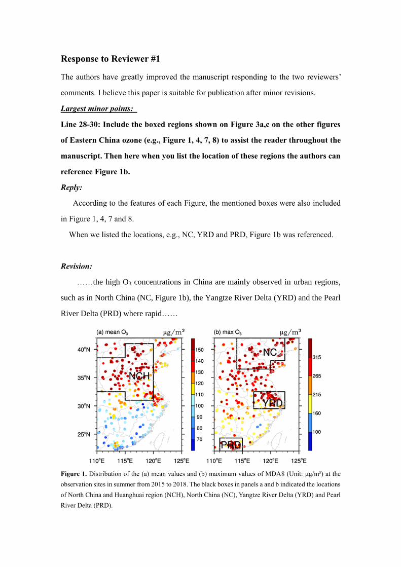
……the high O3 concentrations in China are mainly observed in urban regions,
such as in North China (NC, Figure 1b), the Yangtze River Delta (YRD) and the Pearl
River Delta (PRD) where rapid……
Figure 1. Distribution of the (a) mean values and (b) maximum values of MDA8 (Unit: μg/m³) at the
observation sites in summer from 2015 to 2018. The black boxes in panels a and b indicated the locations
of North China and Huanghuai region (NCH), North China (NC), Yangtze River Delta (YRD) and Pearl
River Delta (PRD).

Figure 2. Anomalies of the summer mean MDA8 (Unit: μg/m³) in 2015 (a), 2016 (b), 2017 (c) and 2018
(d), relative to the mean during 2015–2018. The black pluses indicate that the maximum MDA8 was
larger than 265 μg/m³. The black boxes in panel b indicated the locations of NC, YRD and PRD, while
that in panel d was the NCH area.

Figure 5. Composites of the MDA8 (Unit: μg/m³) for PAT1 (a, b) and PAT2 (c, d) in summer from 2015
to 2018. Panels (a) and (c) were composited when the time coefficient of EOF1 and EOF2 was greater
than one standard deviation, while panels (b) and (d) were composited when the time coefficient was less
than –1×one standard deviation. The black box in panel a-b indicated the location of NCH, while those
in panel c-d were the NH, YRD and PRD area.

Figure 8. The first (a, c, e, g) and second (b, d, f, h) EOF spatial patterns of MDA8 in summer in
2015 (a, b), 2016 (c, d), 2017, (e, f) and 2018(g, h). The percentage number in panels (a, c, e, g) and (b,
d, f, h) are the variance contributions of the first and second EOF mode. The black boxes indicated the
location of NCH, NH, YRD and PRD, respectively.
Line 111: Do you think the high levels of MDA8 around the large cities has to do
with aged pollutant transport in the cities, which may be related to lower O3 in
the cities due to NOx titration but outside of the cities the air was in a different
NOx regime and O3 increased? This idea has been largely absent from this paper,
but I believe it is worth discussing.
Reply:
The related discussions were added in the revised manuscripts, e.g., in the
Introduction, the first paragraph of Section 3, and in the Conclusions and Discussions.
Revision in the Introduction:
……Although deep stratospheric intrusions may elevate surface ozone levels (Lin
et al., 2015), the main source of surface ozone is the photochemical reactions between
the oxides of nitrogen (NOx) and volatile organic compounds (VOC), i.e., NOx + VOC
= O3. The concentrations of NOx and VOC are fundamental drivers impacting ozone
production, and are sensitive to the regime of ozone formation, i.e., NOx-limited or
VOC-limited (Jin and Holloway 2015)……
Revision in the first paragraph of Section 3:
……Surface O3 pollution was closely linked to the anthropogenic emissions that
dispersed and concentrated in the large cities (Fu et al., 2012), which was similar to the
haze pollution (Yin et al., 2015). In the megacity cluster, the photochemical regime for
ozone formation is combination of NOx-limited and VOC-limited regimes (Jin and
Holloway 2015). In the YRD and PRD, high levels of MDA8 were scattered around the
large cities. Due to high emissions of NOx both in large and small cities in the NCH
region, the high-level O3 values were contiguous, indicating extensively surface O3
pollution (Figure 1)……
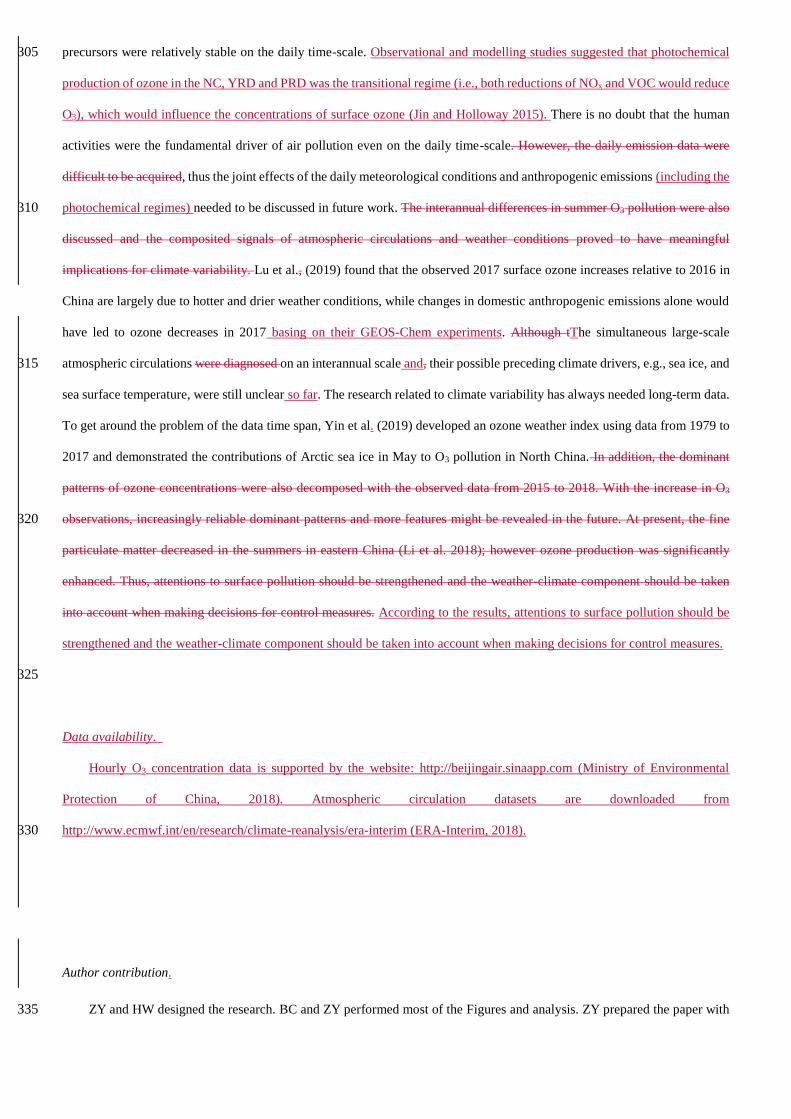
Revision in the Conclusions and Discussions:
……In this study, we mainly emphasized the contribution of the meteorological
impacts and assumed the emissions of ozone precursors were relatively stable on the
daily time-scale. Observational and modelling studies suggested that photochemical
production of ozone in the NC, YRD and PRD was the transitional regime (i.e., both

reductions of NOx and VOC would reduce O3), which would influence the
concentrations of surface ozone (Jin and Holloway 2015). There is no doubt that the
human activities were the fundamental driver of air pollution even on the daily time-
scale, thus the joint effects of the daily meteorological conditions and anthropogenic
emissions (including the photochemical regimes) needed to be discussed in future
work……
Line 116: Severe O3 pollution is mentioned a few times in the paper but “severe”
is not defined as a threshold. What do the authors mean by this? Is it anything
above “Moderately polluted”?
Reply:
Most of the uses of “severe” were replaced by more accurate presentations, such
as “high levels of O3 pollutions”, “heavily polluted O3 pollutions” and “high
concentrations of O3”, etc.
Revision :
Line 139: The authors focus the discussion of PAT2 on NC and YRD, with the
occasional mention to PRD (e.g., line 207-208). Often there are places where the
comment applies to both YRD and PRD (e.g., Lines 146, 181-202) and could be
included. Is there a reason why not to include it in the discussion of PAT2?
Reply:
From the mean MDA8 (Figure 1a), the composites for PAT2 (Figure 4), the ozone
concentrations in PRD were not as high as those in the NC and YRD areas. Thus, we
did not pay much attentions on PRD region. Particularly, in the “Associated
atmospheric circulations”, we did not mention the ozone pollution in PRD.
However, when analyzing the observational features, we also included the ozone
in PRD to show some new features.
Lines 223-251: I am not convinced by the discussion of Figures 10 and 11 as this is
one year being compared to a really small sample size of a four-year average which
includes that same one year. It is the nature of the availability of the data that the
authors choose not to extend their analysis further back. I think the paper can
stand alone without these two additional figures and discussion. This could be
revisited after more time has passed in a later publication.
Reply:
According to the reviewer’s comment, we decided to cancel the Figure 10 and 11.
We now focus on the dominant patterns and their varying features in different years.
Some new works will be supplemented and we will revisit the Figure 10 and Figure 11
in a later manuscript.
The contents related to Figure 7–9 were rewritten and redistributed in the revised
version. The texts associated Figure 10 &11 were deleted. Detailed revisions can be
found in the revised manuscript and also the mark-up manuscript.
Minor and technical comments:
Line 22: Start off the first sentence with something like “High levels of ozone occur
both in the stratosphere and at the ground level”. Otherwise ozone occurs
throughout the troposphere, just not always at unhealthy concentrations.
Reply:
According to the reviewer’s comment, this sentence was revised.
Revision:
Line 34: I do not understand the significance of the greater ozone trend on the
highest mountain in NC. This indicates to me that the background ozone in the
free troposphere in the region is possibly increasing. Is this what the authors mean?
Please clarify the significance of this statement.
Reply:
What we meant is that the increasing trend was widespread in the east of China
and it is meaningful to study the variations in ozone pollution in this region.
Furthermore, after your reminder, we thought the increasing trend partly indicate the
background ozone in the free troposphere in the region is possibly increasing.
Referencing the reviewer’s suggestion, we revised the statement as follows.
Revision:
……Although far away from the anthropogenic emissions, the summer (June-
July-August, JJA) O3 on the highest mountain over NC (Mount Tai) increased
significantly by 2.1 ppbv yr−1 from 2003 to 2015 (Sun et al., 2016)……
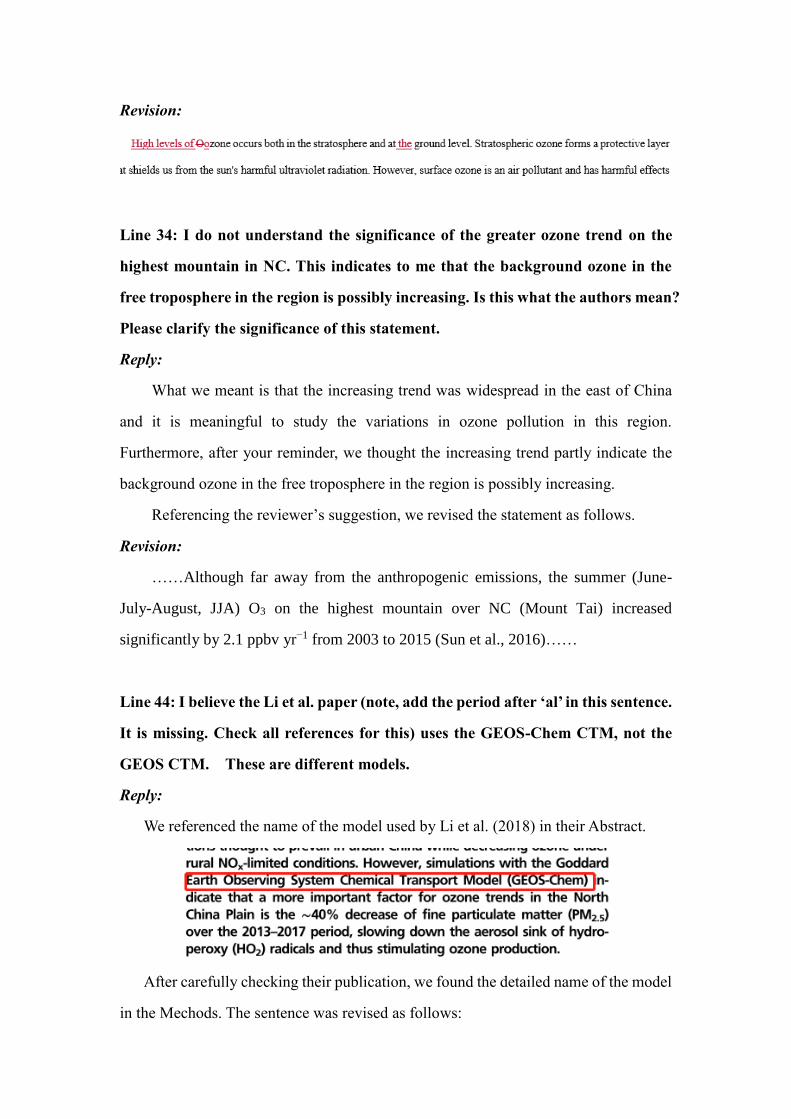
Line 44: I believe the Li et al. paper (note, add the period after ‘al’ in this sentence.
It is missing. Check all references for this) uses the GEOS-Chem CTM, not the
GEOS CTM. These are different models.
Reply:
We referenced the name of the model used by Li et al. (2018) in their Abstract.
After carefully checking their publication, we found the detailed name of the model
in the Mechods. The sentence was revised as follows:
Revision:
……Employed the GEOS-Chem chemical transport model, Li et al. (2018) found
that rapid decreases in fine particulate matter levels significantly stimulated ozone
production in NC by slowing down the aerosol sink of hydro-peroxy radicals……
Line 57: Can the authors provide a summary sentence at the end of this paragraph
linking all these studies together?
Reply:
According to the reviewer’s comment, a summary sentence was supplemented.
Revision:
……Thus, in addition to human activities and secondary aerosol processes, the
impacts of atmospheric circulations and meteorological conditions must be
systematically studied to improve understanding of the O3 pollution in North
China……
Line 58-59: The authors claim that Wang et al. (2017) claim the study uses ozone
data from prior to 2010. How can the reader then assume that the 7 referenced
studies in the paragraph above with publication dates prior to 2019 are using
recent enough ozone data to that the authors can use these papers to make their
claims?
Reply:
To avoid the confusions, we deleted this sentence.
Revision:
Line 62: I know I asked how your study is different to the Zhao and Wang (2017)
paper, but stating “Actually, in our study, we found the ….” comes out of nowhere
compared to the rest of your introduction. Please modify this sentence to be less
aggressive and more like, “In this study, we built upon the previous literature
analyzing ozone and meteorological influences thanks to the availability of more
ozone observations by the Chinese government since 2015, providing us more
information to analyze then available in these earlier studies, e.g., Zhao and Wang
(2017).”
Reply:
Thanks to the kind remind from the reviewer. We worried too much to show the
differences between our studies and Zhao and Wang (2017) and now follow the
reviewer’s suggestions.
Revision:
The dominant patterns of daily ozone in summer in east of China are still unclear.
In this study, we built upon the previous literature analysing ozone and meteorological
influences thanks to the availability of more ozone observations by the Chinese
government since 2015, providing us more information to analyse than available in
these earlier studies, e.g., Zhao and Wang (2017).
Line 73: What threshold was used to unify the sites? For example, did some sites
move location but still considered as one time series?
Reply:
The sites with missing data >5% were removed and there were 868 sited were kept
in the four years.
Line 80: Thank you for adding this detail. However, I am not used to this type of
notation; is there a reason some left brackets are curved ( and not [ ?
Reply:
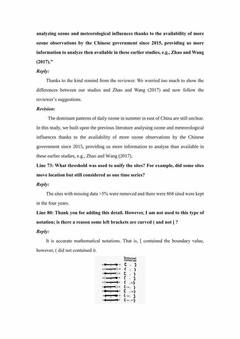
It is accurate mathematical notations. That is, [ contained the boundary value,
however, ( did not contained it.

Line 82: Can you provide a link either here in the text or at the end of the paper
in a “Data Availability” section to where you got the ERA-Interim data.
Reply:
Data Availability was added as the ACP journal required.
Revision:
Data availability.
Hourly O3 concentration data is supported by the website:
http://beijingair.sinaapp.com (Ministry of Environmental Protection of China, 2018).
Atmospheric circulation datasets are downloaded from
http://www.ecmwf.int/en/research/climate-reanalysis/era-interim (ERA-Interim, 2018).
Line 83: Remove at to read “temperature from surface to 100 hPa”.
Reply:
The errors were corrected.
Revision:
Line 86, 89-90: (1) I am still confused by this description of reanalysis timesteps to
Beijing time. How many 6-hourly reanalysis timestamps are used in the daytime
data analysis? Why are there different time period for the 3-hourly data than 6
hourly data? Can you use the same time period but just more 3-hourly data?
(2) 00 am to 00pm UTC does not make sense. I think you mean 00 UTC to 12 UTC
which would mean you have 3 6-hourly timesteps (00, 06, 12 UTC). The am and
pm should also be removed from the 21 UTC to 09 UTC. And this means you have
5 3hourly timesteps (21, 00, 03, 06, 09 UTC). Why is this offset 3 hours from the 6-
hourly timesteps (could have done 00,03,06,09, 12 UTC)?
Reply:
(1) The required answers were clearly shown on the website of ERA-Interim
(https://confluence.ecmwf.int/pages/viewpage.action?pageId=56658233). On the page

about “ERA-Interim: 'time' and 'steps', and instantaneous, accumulated and min/max
parameters”, we can found the explanations about the parameters.
ERA-Interim data is archived at website differently according to whether they are
produced by the analysis (An), or the forecast (Fc), and timesteps of data which we
could get is shown in Fig R1. Only precipitation and surface solar are produced by
forecast in all the data which we used, which was illustrated in Table 8 and 9 of
Berrisford et al. (2011). Fc data is the accumulated (from the beginning of the forecast)
and can be treated as 3-hr data due to 4 timesteps in 12 hours, and An data is
instantaneous (Berrisford et al., 2011).
We wanted to research the link between atmospheric circulation and MDA8 which
mostly occurs in daytime (8:00 a.m. to 8:00 p.m. Beijing Time). For Fc, we considered
00 UTC to 12UTC (8:00 to 20:00 Beijing Time), the upper way in Figure R1, (first
‘+12’ line in Fig. R1) as daytime in Beijing. It means we just use 1 timesteps data which
is accuunulated from 00 UTC to 12 UTC. But for An (second line in Fig. R1), we could
only calculate the mean of 00:00 and 06:00 UTC as daytime mean and it represent mean
of the time-scale 3-hour (half of the timesteps) before the 00:00 to 3-hour after 06:00.
It means that daytime is 21 UTC to 9 UTC (5:00 to 17 Beijing Time).
Figure R1. ERA-interim Data timesteps (downloaded from the ERA website).
Reference:
Berrisford, P, Dee, DP, Poli, P, Brugge, R, Fielding, M, Fuentes, M, Kållberg, PW,
Kobayashi, S, Uppala, S, Simmons, A, The ERA-Interim archive Version 2.0.
https://www.ecmwf.int/node/8174.

(2) The timing way was changed to 24HR way.
Revision:
……Due to the different representative period of each element in ERA-Interim
data, the daytime for Z, wind, relative humidity, vertical velocity, air temperature and
cloud cover was from 05 to 17 (Beijing Time; 21–09 UTC), while it is from 08 to 20
(Beijing Time; 00 to 12 UTC) for precipitation and downward solar radiation……
Line 94: remove ‘ly’ from relatively
Reply:
The errors were corrected.
Revision:
Line 104: I suggest changing this sentence to “….was mostly lower than 100 ug/m3,
and lower than the O3 pollution in North China and in the Huanghuai area (NCH,
about 31-41N, 110-120E)”. This modifies the second half of the sentence as well as
adding in the box region for the NCH (which I guessed from Figure 3).
Reply:
The errors were corrected.
Revision:
Line 112: are cities large and small based on population or area-covered?
Reply:
The large and small cites are distinguished based on population.

Line 115: Could highlight that this threshold is matching the list now given in line
80-81; e.g., change to ….the threshold of “heavily O3 pollution” in China…
Reply:
According to the reviewer’s advice, this sentence was improved.
Revision:
Line 118: Are these cities with large populations “Megacities”?
Reply:
Yes, these cities with large populations are megacities. To emphasize the large
populations, we maintained the presentation.
Line 119: How often was the MDA8 value nearly above 100 ug/m3? Are you trying
to say the ozone was hardly below 100 ug/m3 on any day in the time series?
Reply:
The detailed percentages were explained in the next sentence.
The percentage of non-O3-polluted days (<100 μg/m³) and moderate O3-polluted
days (>215 μg/m³) were 14.9% and 15.5% for the mean MDA8 of these three cities.
Line 122: What does “exceeded the health threshold” in reference to? Is that
“Good” and above?
Reply:
It is the upper limit “Excellent” level.
Revision:
Line 127: Change reference to (Figure 2a,b)
Reply:
The sentence was corrected.
Revision:
Line 141: There looks to be extra spacing in front of -1x
Reply:
The errors were corrected.
Revision:
……less than –1×one standard deviation…..
Line 142: Change showed to shows. There are other places where the authors
switch back and forth between verb tenses (e.g., Line 154, 159).
Reply:
Similar errors were checked and corrected throughout the manuscript.
Line 145: add (Fig 4a, b) after “respectively”.
Reply:
The reference of Figure were added.
Revision:
Line 149: change recent four years to “the four years of study” since this becomes
less true after publication.
Reply:
The errors were corrected.
Revision:
Line 150: What does “were reasonably supposed to be relatively stable on the daily
time-scale” mean. I think change to “Despite the economic productions and
human activities steadily increasing from 2015 to 2018 in Eastern China, we
assume the emissions of ozone precursors to be relatively stable on the daily time-
scale”.
Reply:
According to the reviewer’s advice, this sentence was improved.
Revision:
In eastern China, despite the economic productions and human actives steadily
increased in the four years of study and we assume the emissions of ozone precursors
to be relatively stable on the daily time-scale.
Line 154-156: I do not feel this “For example,” sentence is necessary.
Reply:
This sentence was deleted.
Revision:
Line 158: so this is stagnation and as such there is the buildup of pollutants too
without removal from weather systems passing by. I do not think that idea has
been discussed.
Reply:
The removal of ozone pollutants by the weather were clearly discussed in the
revised manuscript, which make our study more complete.
Revision in the Abstract:

Revision in Section 4:
Revision in Conclusion:
Line 159: Start sentence with “In Figure 5a, there are negative …”
Reply:
This sentence started with “In Figure 6a” now.
Revision:
Line 163: Change to “(EAT, Table 1)”
Reply:
According to the reviewer’s advice, this sentence was improved.
Revision:
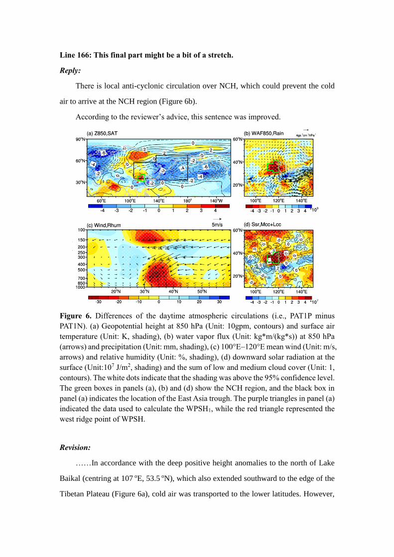
Line 166: This final part might be a bit of a stretch.
Reply:
There is local anti-cyclonic circulation over NCH, which could prevent the cold
air to arrive at the NCH region (Figure 6b).
According to the reviewer’s advice, this sentence was improved.
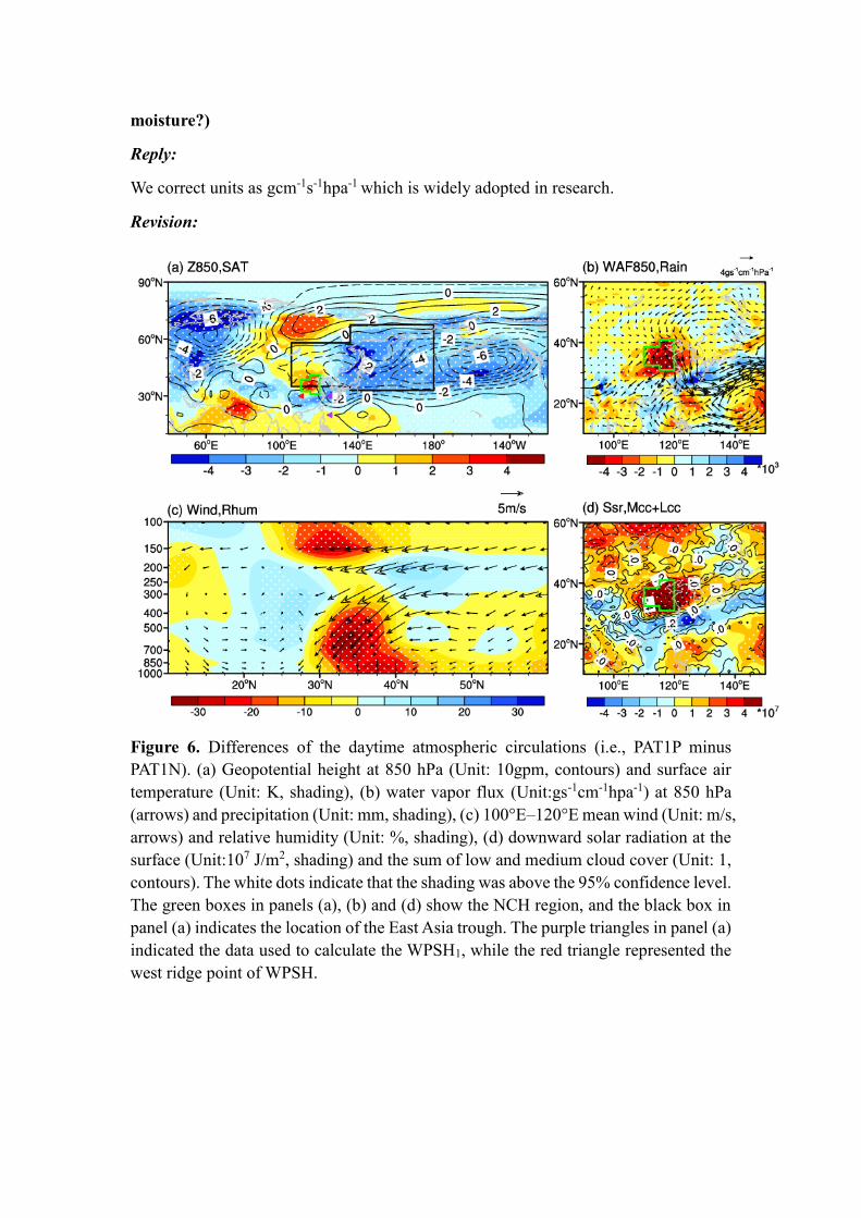
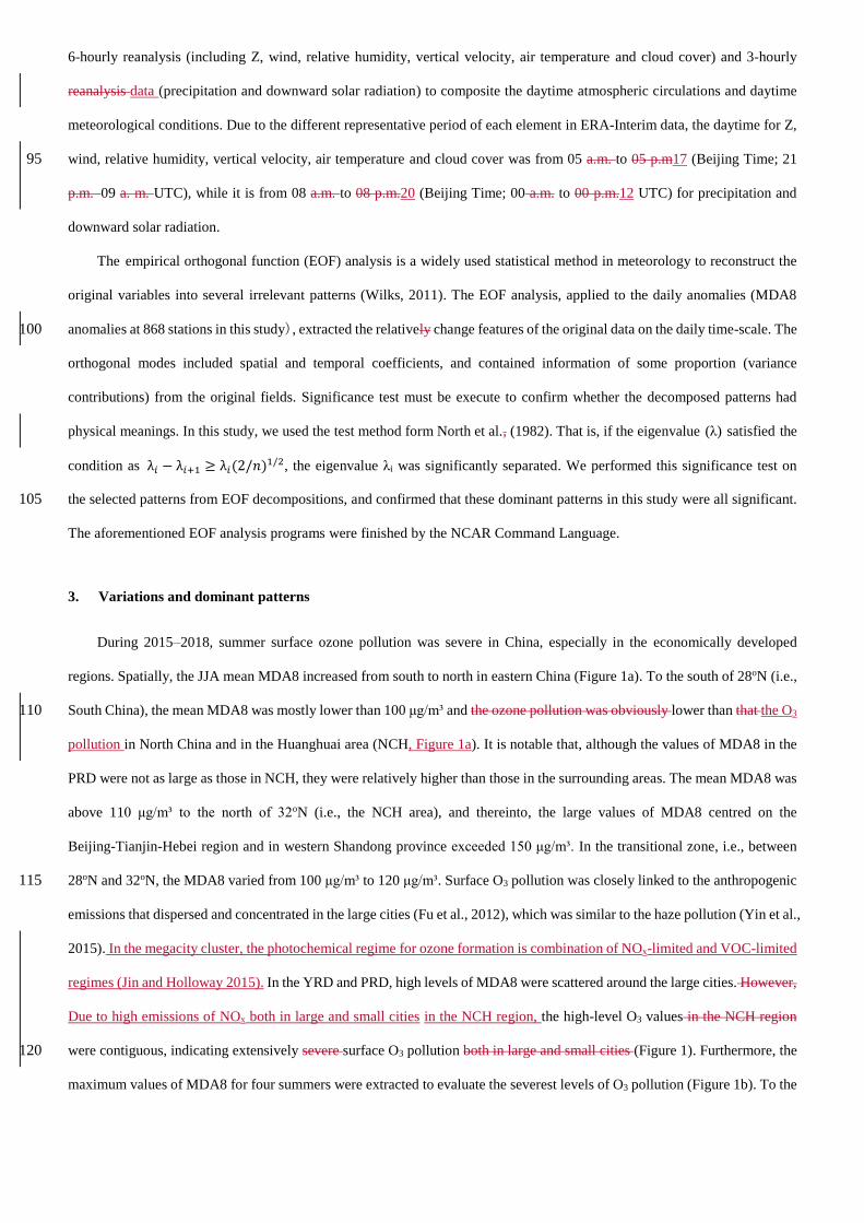
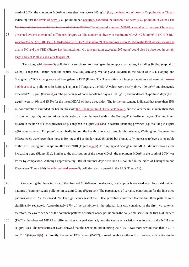
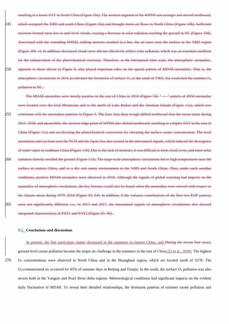
Figure 6. Differences of the daytime atmospheric circulations (i.e., PAT1P minus
PAT1N). (a) Geopotential height at 850 hPa (Unit: 10gpm, contours) and surface air
temperature (Unit: K, shading), (b) water vapor flux (Unit: kg*m/(kg*s)) at 850 hPa
(arrows) and precipitation (Unit: mm, shading), (c) 100°E–120°E mean wind (Unit: m/s,
arrows) and relative humidity (Unit: %, shading), (d) downward solar radiation at the
surface (Unit:107 J/m2, shading) and the sum of low and medium cloud cover (Unit: 1,
contours). The white dots indicate that the shading was above the 95% confidence level.
The green boxes in panels (a), (b) and (d) show the NCH region, and the black box in
panel (a) indicates the location of the East Asia trough. The purple triangles in panel (a)
indicated the data used to calculate the WPSH1, while the red triangle represented the
west ridge point of WPSH.
Revision:
……In accordance with the deep positive height anomalies to the north of Lake
Baikal (centring at 107 oE, 53.5 oN), which also extended southward to the edge of the
Tibetan Plateau (Figure 6a), cold air was transported to the lower latitudes. However,
local anti-cyclonic circulation over NCH prevented the cold air to arrive at the NCH
region (Figure 6b).……
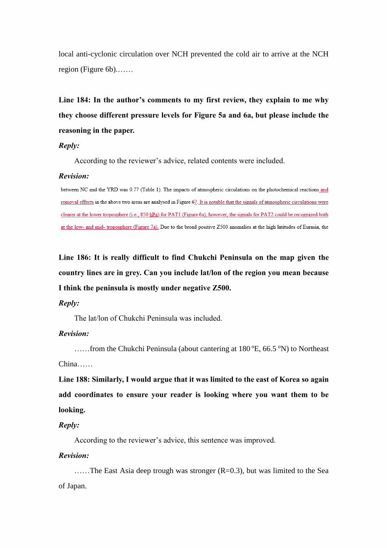
Line 184: In the author’s comments to my first review, they explain to me why
they choose different pressure levels for Figure 5a and 6a, but please include the
reasoning in the paper.
Reply:
According to the reviewer’s advice, related contents were included.
Revision:
Line 186: It is really difficult to find Chukchi Peninsula on the map given the
country lines are in grey. Can you include lat/lon of the region you mean because
I think the peninsula is mostly under negative Z500.
Reply:
The lat/lon of Chukchi Peninsula was included.
Revision:
……from the Chukchi Peninsula (about cantering at 180 oE, 66.5 oN) to Northeast
China……
Line 188: Similarly, I would argue that it was limited to the east of Korea so again
add coordinates to ensure your reader is looking where you want them to be
looking.
Reply:
According to the reviewer’s advice, this sentence was improved.
Revision:
……The East Asia deep trough was stronger (R=0.3), but was limited to the Sea
of Japan.
Line 194: Remove the word obvious.
Reply:
According to the reviewer’s advice, this sentence was improved.
Revision:
Line 204: Change “the past four years” to “these past four years” as this will
change after publication.
Reply:
According to the largest minor comment to Figure 10 & 11, the related sentence
was already deleted.
Line 217: Could include a reference to Fig 8.
Reply:
According to the largest minor comment to Figure 10 & 11, the related sentence
was already deleted.
The following are the reasons why I do not think Figures 10 and 11 add to the
manuscript:
Line 223: change to “were generally negative”. I think there is a mix of positive
and negative in the YRD in Figure 7b, not strictly positive as is written.
Line 227: Again, I see a ridge over Chukchi Peninsula, not a trough, so include
coordinates of where you want the reader to be looking.
Line 229: Both Figure 10 and 11 could have the same purple arrows to identify
how the authors would calculate the WPSH as in Figures 5 and 6. Again, authors
could include coordinates or a box region as in Figures 5 and 6 to indicate the
location of EAT and WPSH.
Line 231: I disagree with the authors that more low to mid-level clouds formed as
it looks to me that the box straddles the zero line and that instead of a decrease in

solar radiation reaching the ground in NC I see positive colors in that box too in
Figure 10d.
Line 236: What do the authors mean by “south of YRD”? Do they mean outside
of the box or the southern portion of the YRD? Does that mean PRD?
Lines 225-237: There are no significant differences near the NC or YRD in any of
the four panels in Figure 10.
Line 238: I do not like how the sentence starts with “-+-“. Can the authors at least
put “The” prior to the symbols? Is this the same as an OMEGA block and could
be written as such instead of -+- ?
Line 243: I do not see an anomalous anticyclone over the NCH in Figure 11a, but
more on the border with cyclonic flow to the southwest and anticyclone to the east,
and as the authors describe later in reference to the water vapor flux, the NCH is
in a region of anomalous divergent flow.
Line 244: When the authors say “it was difficult to form cloud” the NCH straddles
the zero line and shows a mix of both positive and negative SSR so how can they
say “more solar radiation directly reach the ground (Figure 11d)”?
Line 247: Out of nowhere the authors mention “signals of global warming”. Such
bold statements in a manuscript, which depend on figures in the supplemental
material, should not be made.
Reply:
According to the largest minor comment to Figure 10 & 11, the related sentence
was already deleted.
We now focus on the dominant patterns and their varying features in different
years. Some new works will be supplemented and we will revisit the Figure 10 and
Figure 11 in a later manuscript. We believe the above comments from the reviewer
will be helpful in our new researches.
The contents related to Figure 7–9 were rewritten and redistributed in the revised
version. The texts associated Figure 10 &11 were deleted. Detailed revisions can be
found in the revised manuscript and also the mark-up manuscript.
Overall the Discussion is fine.
Line 254: Add a reference (e.g. Li et al., 2018) to the end of the opening sentence,
possibly bringing over the point made at the end of the discussion on line 281 “At
present, the fine PM decreased in the summers in eastern China….”
Reply:
According to the reviewer’s advice, this sentence was improved.
Revision:
At present, the fine particulate matter decreased in the summers in eastern China,
and ground-level ozone pollution became the major air challenge in the summers in the
east of China (Li et al., 2018).
Line 264: the increased SAT and thus decreased cold air advection from the north
a) seems backwards (less cold air advection would likely lead to increased SAT at
lower latitudes) and b) the negative Z500 to the west with flow from south and
southwest likely brought warmer temperatures from the southern latitudes into
the region.
Reply:
According to the reviewer’s advice, this sentence was improved.
Revision:
……positive geopotential height anomalies at the high latitudes significantly
decreased cold air advection from the north and thus increased the surface air
temperature……
Line 270: “…daily emission data were difficult to be acquired” implies the authors
have acquired such data. Is that true or are these data difficult to acquire?
Reply:
It is true these are difficult to acquire. To avoid such confusions, we revised this
sentence.
Revision:
……There is no doubt that the human activities were the fundamental driver of air

pollution even on the daily time-scale, thus the joint effects of the daily meteorological
conditions and anthropogenic emissions needed to be discussed in future work……
Line 273: remove the comma before (2019).
Reply:
The errors were corrected.
Revision:
……Lu et al. (2019) found that……
Line 275: How were the “domestic anthropogenic emissions alone would have led
to ozone decreases” determined by the Lu et al. study?
Reply:
Lu et al. (2019) based on series of GEOS-Chem experiments and gave such
conclusions.
According to the reviewer’s advice, this sentence was improved.
Revision:
Line 277: Is “were still unclear” in reference to your work presented here or in
reference to the Lu et al. study?
Reply:
According to the reviewer’s advice, this sentence was improved.
Revision:
……The simultaneous large-scale atmospheric circulations on an interannual
scale and their possible preceding climate drivers, e.g., sea ice, and sea surface
temperature, were still unclear so far……

Figure comments:
Figure 2: Can NC, NCH, YRD, and PRD be added to the Figure caption in a
similar fashion to how it was added to the Comments to the Reviewer (Page 47).
Also, could add a reference to Figure S2 in the caption to remind readers to look
there for the locations of these cities.
Reply:
According to the reviewer’s advice, this Figure caption was improved.
Revision:
Figure 3. Variations in MDA8 (Unit: μg/m³) of polluted cities from 2015 to 2018,
including (a) Beijing (capital of China), Tianjin and Tangshan near the capital city;
(b) Taiyuan, Weifang and Shijiazhuang in the south of NCH; (c) Shanghai and Nanjing
in YRD; and (d) Zhongshan and Guangzhou in PRD. The cities in panels (a)-(d) were
located from north to south and were illustrated in Figure S2. The horizontal dash
lines indicated the value of 100 μg/m³ and 215 μg/m³.
Figure 3: Add to Figure 3 caption what the dashed lines in panels b and d represent.
I assume horizontal are the standard deviation and the vertical separate the years.
Reply:
According to the reviewer’s advice, this Figure caption was improved.
Revision:
Figure 4. The first EOF pattern (PAT1: a, b) and second EOF pattern (PAT2: c, d) of
MDA8 in summer from 2015 to 2018, including the spatial pattern (a, c) and the time
coefficient (b, d). The black boxes in panels a and c are the selected North China and
Huanghuai region (NCH), North China (NC), Yangtze River Delta (YRD) and Pearl
River Delta (PRD). The EOF analysis were applied to the daily MDA8 anomalies at
868 stations to extract the relatively change features of the original data on the daily
time-scale. The percentages on panel (b) and (d) were the variance contributions of the
first and second EOF mode. The horizontal dash lines indicated one standard
deviation, and the vertical ones separated the years.
Figure 5, 6, 10, 11: The units for water vapor flux are written as kg*m/(kg*s) which
is a bit odd. I strongly encourage the authors to use negative values to indicate
denominators in units throughout the paper. This would change these units to kg
m kg-1 s-1 which then leads me to my next question whether these are the correct
units. In its current form are the kg’s representing different things (dry air vs
moisture?)
Reply:
We correct units as gcm-1s-1hpa-1 which is widely adopted in research.
Revision:
Figure 6. Differences of the daytime atmospheric circulations (i.e., PAT1P minus
PAT1N). (a) Geopotential height at 850 hPa (Unit: 10gpm, contours) and surface air
temperature (Unit: K, shading), (b) water vapor flux (Unit:gs-1cm-1hpa-1) at 850 hPa
(arrows) and precipitation (Unit: mm, shading), (c) 100°E–120°E mean wind (Unit: m/s,
arrows) and relative humidity (Unit: %, shading), (d) downward solar radiation at the
surface (Unit:107 J/m2, shading) and the sum of low and medium cloud cover (Unit: 1,
contours). The white dots indicate that the shading was above the 95% confidence level.
The green boxes in panels (a), (b) and (d) show the NCH region, and the black box in
panel (a) indicates the location of the East Asia trough. The purple triangles in panel (a)
indicated the data used to calculate the WPSH1, while the red triangle represented the
west ridge point of WPSH.

Figure 7. Differences of the daytime atmospheric circulations (i.e., PAT2P minus
PAT2N). (a) Geopotential height at 500 hPa (Unit: 10gpm, contours) and surface air
temperature (Unit: K, shading), (b) water vapor flux (Unit:gs-1cm-1hpa-1) at 850 hPa
(arrows) and precipitation (Unit: mm, shading), (c) 100°E–120°E mean wind (Unit: m/s,
arrows) and relative humidity (Unit: %, shading), (d) downward solar radiation at the
surface (Unit: 107J/m2, shading) and the sum of low and medium cloud cover (Unit: 1,
contours). The white dots indicate that the shading was above the 95% confidence level.
The green boxes in panel (a), (b) and (d) are the NC and YRD regions, and the black
box in panel (a) indicates the location of the East Asia trough. The purple triangles in
panel (a) indicated the data used to calculate the WPSH2.
Figure 7: It is difficult to see the crosses when the O3 anomaly is less than -25 ppb
(the dark blue color). Can that be adjusted? Or maybe have white crosses instead?
Also the y-axis minor tick marks are an odd spacing compared to the major 5
degree labelled tick marks. Can these minor tick marks be changed to maybe every
1 degree?
Reply:
According to the reviewer’s advice, the Figure 5 was re-plotted. For example, the
color bar was re-scaled and the label marks of y-axis was re-divided.

Revision:
Figure 2. Anomalies of the summer mean MDA8 (Unit: μg/m³) in 2015 (a), 2016 (b),
2017 (c) and 2018 (d), relative to the mean during 2015–2018. The black pluses indicate
that the maximum MDA8 was larger than 265 μg/m³.
Figure 9: Are the variations in reference to an average for all available sites in the
NC and the YRD regions? If so, please add this level of detail to the Figure 9
caption.
Reply:
According to the reviewer’s advice, this Figure caption was improved.
Revision:
Figure 9. Variations in the MDA8 (Unit: μg/m³) of NC (black) and the YRD (blue) in
2016 (a) and 2018 (b). The MDA8 was calculated as an average for all available
sites in the NC and the YRD regions.

Response to Reviewer #2
The quality of the manuscript has been improved. The revised manuscript is much
easier to follow, and the figures are carefully labeled and explained. Overall the authors
have well addressed my concerns, but I’m confused with the authors’ reply to my first
comment regarding the impact of anthropogenic emissions.
In the first point, the authors clarify they are more interested in the fluctuation of
MDA8 ozone, but the inter-annual variations in emissions should also have
impacts on the anomalies of MDA8 ozone.
In the second point, the authors argue that the emissions are stable at daily scale
and it’s hard to acquire daily emission data, but I don’t think this argument
justifies why the impacts of emissions on the inter-annual variability of ozone (i.e.
Figure 7) are not accounted. I'd suggest the authors provide some discussions on
how the recent decreasing trends of NOx emissions could impact on the inter-
annual variability of ozone.
Reply:
(1) As regards the mechanisms, our study mainly focus on the impacts of
meteorological conditions on daily time-scale.
(2) The discussion of the impact of decreasing trends of NOx was really absent,
which was strengthened in the revised manuscript and can be found in the following
revisions.
(3) According to the other reviewer’s comment, we decided to delete the
Figure 10 and 11, i.e., the iner-annual variability of ozone was not discussed in this
revised version. We now focus on the dominant patterns and their varying features in
different years. Some new works will be supplemented and we will revisit the Figure
10 and Figure 11 in a later manuscript.
The contents related to Figure 7–9 were rewritten and redistributed in the revised
version. The texts associated Figure 10 &11 were deleted. Detailed revisions can be
found in the revised manuscript and also the mark-up manuscript.

Revision in the Introduction:
……Although deep stratospheric intrusions may elevate surface ozone levels (Lin
et al., 2015), the main source of surface ozone is the photochemical reactions between
the oxides of nitrogen (NOx) and volatile organic compounds (VOC), i.e., NOx + VOC
= O3. The concentrations of NOx and VOC are fundamental drivers impacting ozone
production, and are sensitive to the regime of ozone formation, i.e., NOx-limited or
VOC-limited (Jin and Holloway 2015)……
Revision in the first paragraph of Section 3:
……Surface O3 pollution was closely linked to the anthropogenic emissions that
dispersed and concentrated in the large cities (Fu et al., 2012), which was similar to the
haze pollution (Yin et al., 2015). In the megacity cluster, the photochemical regime for
ozone formation is combination of NOx-limited and VOC-limited regimes (Jin and
Holloway 2015). In the YRD and PRD, high levels of MDA8 were scattered around the
large cities. Due to high emissions of NOx both in large and small cities in the NCH
region, the high-level O3 values were contiguous, indicating extensively surface O3
pollution (Figure 1)……
Revision in the Conclusions and Discussions:
……In this study, we mainly emphasized the contribution of the meteorological
impacts and assumed the emissions of ozone precursors were relatively stable on the
daily time-scale. Observational and modelling studies suggested that photochemical
production of ozone in the NC, YRD and PRD was the transitional regime (i.e., both
reductions of NOx and VOC would reduce O3), which would influence the
concentrations of surface ozone (Jin and Holloway 2015). There is no doubt that the
human activities were the fundamental driver of air pollution even on the daily time-
scale, thus the joint effects of the daily meteorological conditions and anthropogenic
emissions (including the photochemical regimes) needed to be discussed in future
work……

Dominant Patterns of Summer Ozone Pollution in Eastern China and
Associated Atmospheric Circulations
Zhicong Yin 12, Bufan Cao1, Huijun Wang12
1Key Laboratory of Meteorological Disaster, Ministry of Education / Joint International Research Laboratory of Climate and
Environment Change (ILCEC) / Collaborative Innovation Center on Forecast and Evaluation of Meteorological Disasters 5
(CIC-FEMD), Nanjing University of Information Science & Technology, Nanjing 210044, China
2Nansen-Zhu International Research Centre, Institute of Atmospheric Physics, Chinese Academy of Sciences, Beijing, China
Correspondence to: Zhicong Yin ([email protected])
Abstract. Surface ozone has been severe during summers in the eastern parts of China, damaging human’s health and flora and
fauna. During 2015–2018, ground-level ozone pollution increased and intensified from south to north. In North China and 10
Huanghuai region, the O3 concentrations were highest. Two dominant patterns of summer ozone pollution were determined,
i.e., a south-north covariant pattern and a south-north differential pattern. The anomalous atmospheric circulations composited
for the first pattern manifested as a zonally enhanced East Asia deep trough and as a west Pacific subtropical high whose
western ridge point shifted northward. The local hot, dry air and intense solar radiation enhanced the photochemical reactions
to elevate the O3 pollution levels in North China and Huanghuai region, however the removal of pollutants were decreased. For 15
the second pattern, the broad positive geopotential height anomalies at high latitudes significantly weakened cold air advection
from the north, and those extending to North China resulted in locally high temperature near the surface. In a different manner,
the west Pacific subtropical high transported sufficient water vapor to the Yangtze River Delta and resulted in locally adverse
environment for the formation of surface ozone. In addition, the most dominant pattern in 2017 and 2018 was different from
that in previous years, which is investigated as a new feature. Furthermore, the implications for the interannual differences in 20
summer O3 pollution have also proven to be meaningful.
1. Introduction
High levels of Oozone occurs both in the stratosphere and at the ground level. Stratospheric ozone forms a protective layer
that shields us from the sun's harmful ultraviolet radiation. However, surface ozone is an air pollutant and has harmful effects
on people and on the environment, such as damaging human lungs (Day et al., 2017) and destroying agricultural crops and 25
forest vegetation (Yue et al., 2017). Worldwide, severe polluted ozone events are more frequent and stronger in China than
those that have taken place in Japan, South Korea, Europe, and the United States (Lu et al., 2018). Due to their close
relationship with anthropogenic emissions (Li et al., 2018), the high O3 concentrations in China are mainly observed in urban
regions, such as in North China (NC, 114°E–122.5°E, 36.5°N–42°NFigure 1b), the Yangtze River Delta (YRD,
117°E–122.5°E, 29.5°N–32.5°N) and the Pearl River Delta (PRD, 111°E–115°E, 22°N–24.3°N) where rapid development has 30

occurred in recent decades (Wang et al., 2017). An increase in surface ozone levels was found in China in 2016 and 2017
relative to 2013 and 2014 (Lu et al., 2018). The O3 pollution levels in Beijing-Tianjin-Hebei (part of NC) were the most severe
in China (Wang et al., 2006; Shi et al., 2015) and this situation has been getting worse. The O3 concentrations in North China
underwent a significant increase in the period of 2005–2015, with an average rate of 1.13±0.01 ppbv yr−1 (Ma et al., 2016).
Although far away from the anthropogenic emissions, Even on the highest mountain over NC, Mount Tai, the summer 35
(June-July-August, JJA) O3 on the highest mountain over NC (Mount Tai) increased significantly by 2.1 ppbv yr−1 from 2003
to 2015 (Sun et al., 2016). The O3 levels generally presented increasing trends from 2012 to 2015 in the YRD (Tong et al.,
2017), e.g., the O3 concentrations in Shanghai (a mega-city) increased by 67% from 2006 to 2015 (Gao et al., 2017). In the
PRD region, O3 increased by 0.86 ppbv yr−1 from 2006 to 2011 (Li et al., 2014). Furthermore, Severe oozone pollution is
projected to increase in the future over eastern China (Wang et al., 2013). 40
Although deep stratospheric intrusions may elevate surface ozone levels (Lin et al., 2015), the main source of surface
ozone is the photochemical reactions between the oxides of nitrogen (NOx) and volatile organic compounds (VOC), i.e., NOx +
VOC = O3. The concentrations of NOx and VOC are fundamental drivers impacting ozone production, and are sensitive to the
regime of ozone formation, i.e., NOx-limited or VOC-limited (Jin and Holloway 2015). The changes in fine particulate matter
are also a pervasive factor for the variation in ozone concentration. Employed the Goddard Earth Observing 45
SystemGEOS-Chem Chemical chemical Transport transport Modelmodel, Li et al. (2018) found that rapid decreases in fine
particulate matter levels significantly stimulated ozone production in NC by slowing down the aerosol sink of hydro-peroxy
radicals. FurthermoreIn addition, the meteorological conditions also influenced the ozone levels via modulation of the
photochemical episodes and removal effects (Yin et al., 2019; Lu et al., 2019). Intense solar radiation accelerated chemical O3
production (Tong et al., 2017). A severe heat wave in the YRD contributed to high O3 concentrations in 2013 (Pu et al., 2017). 50
Winds had an impact on the O3 and its precursors at downwind locations (Doherty et al., 2013). Local meteorological
influences are always related to specific large-scale atmospheric circulations. The changes in the East Asian summer monsoon
led to 2–5% interannual variations in surface O3 concentrations over central eastern China (Yang et al., 2014). Continental
anticyclones created sunny and calm weather, which are favourable conditions for O3 production in NC (Ding et al., 2013; Yin
et al., 2019). Due to the associated transports of pollution from inland, tropical cyclones are often related to the evaluation of 55
surface O3 levels in the coastal areas of PRD (Ding et al., 2004). Basing on a case study in 2014, further studies showed that a
strong west Pacific subtropical high (WPSH) was unfavourable for the formation of O3 in South China (Zhao and Wang, 2017),
however the physical mechanisms to impact O3 in North China was still not sufficiently explained. Thus, in addition to human
activities and secondary aerosol processes, the impacts of atmospheric circulations and meteorological conditions must be
systematically studied to improve understanding of the O3 pollution in North China. 60
Wang et al. (2017) reviewed the meteorological influences on ozone events, but the referenced findings were published

mainly before 2010, when measurements in China were still scarce. Since 2015, O3 measurements in eastern China were
steadily and widely implemented, but the O3-weather studies mainly focused on meteorological elements (e.g. temperature,
precipitation etc.) and several synoptic processes (Xu et al., 2017; Xiao et al., 2018; Pu et al., 20137). The dominant patterns of
daily ozone in summer in east of China are still unclear. In this study, we built upon the previous literatures analysing ozone 65
and meteorological influences thanks to the availability of more ozone observations by the Chinese government since 2015,
providing us more information to analyse than available in these earlier studies, e.g., Zhao and Wang (2017)Actually, in our
study, we found the most dominant pattern was different with that in Zhao and Wang (2017) and the dominant patterns also
showed interannual variations. The findings of this study basically help to understand the varying features of daily surface
ozone pollution in eastern China and, their relationships with large-scale atmospheric circulations and the implications for the 70
climate variability.
2. Data sets and methods
Nationwide hourly O3 concentration data since May 2014 are publicly available on http://beijingair.sinaapp.com/. Since
the severe air pollution events in 2013, the air pollution issues gained more attentions from the Chinese government and society,
which aided to start the extensive constructions of operational monitoring stations of atmospheric components and resulted in 75
continuous increasing number of sites (Figure S1). The number of sites in eastern China (110oE–125oE, 22oN–42oN) was 677,
937, 937, 995 and 1007 from 2014 to 2018. It is obvious that the data in 2014 were deficient, while the observations were
broadly distributed in eastern China and continuously achieved since 2015. Thus, the summer O3 data from 2015 to 2018 were
processed (e.g., unifying the sites and eliminating the missing value) and 868 sites in eastern China were employed here to
reveal some new features of surface ozone pollutions and associated anomalous atmospheric circulations. Generally, severe air 80
pollutions occurred more frequently in cites than in rural areas, therefore, the monitoring sites of atmospheric components
mostly gathered around the urban areas, indicating the results of this study were more suitable to for the urban O3 pollution.
The maximum daily average 8 h concentration of ozone (MDA8) is the maximum of the running 8 h mean O3 concentration
during an entire 24 hour day. According to the Technical Regulation on Ambient Air Quality Index of China (the Ministry of
Environmental Protection of China, 2012), MDA8 is generally used to represent the daily O3 conditions. The MDA8 ∈ [0, 85
100], (100, 160], (160, 215], (215, 265], (265, 800] μg/m³ corresponds to “Excellent”, “Good”, “Lightly polluted”,
“Moderately polluted”, “Heavily polluted” levels of air quality in China.
The 2.5°×2.5° ERA-Interim data used here include the geopotential height (Z) at 850 and 500 hPa, zonal and meridional
wind, relative humidity, vertical velocity, air temperature at from surface to 100 hPa, surface air temperature (SAT) and wind,
downward solar radiation at the surface, low and medium cloud cover and precipitation (Dee et al., 2011). Because the 90
maximum photochemical activity often occurred at afternoon (Wang et al., 2010), the daytime data were calculated by the
6-hourly reanalysis (including Z, wind, relative humidity, vertical velocity, air temperature and cloud cover) and 3-hourly
reanalysis data (precipitation and downward solar radiation) to composite the daytime atmospheric circulations and daytime
meteorological conditions. Due to the different representative period of each element in ERA-Interim data, the daytime for Z,
wind, relative humidity, vertical velocity, air temperature and cloud cover was from 05 a.m. to 05 p.m17 (Beijing Time; 21 95
p.m.–09 a. m. UTC), while it is from 08 a.m. to 08 p.m.20 (Beijing Time; 00 a.m. to 00 p.m.12 UTC) for precipitation and
downward solar radiation.
The empirical orthogonal function (EOF) analysis is a widely used statistical method in meteorology to reconstruct the
original variables into several irrelevant patterns (Wilks, 2011). The EOF analysis, applied to the daily anomalies (MDA8
anomalies at 868 stations in this study), extracted the relatively change features of the original data on the daily time-scale. The 100
orthogonal modes included spatial and temporal coefficients, and contained information of some proportion (variance
contributions) from the original fields. Significance test must be execute to confirm whether the decomposed patterns had
physical meanings. In this study, we used the test method form North et al., (1982). That is, if the eigenvalue (λ) satisfied the
condition as λ𝑖 − λ𝑖+1 ≥ λ𝑖(2/𝑛)1/2, the eigenvalue λi was significantly separated. We performed this significance test on
the selected patterns from EOF decompositions, and confirmed that these dominant patterns in this study were all significant. 105
The aforementioned EOF analysis programs were finished by the NCAR Command Language.
3. Variations and dominant patterns
During 2015–2018, summer surface ozone pollution was severe in China, especially in the economically developed
regions. Spatially, the JJA mean MDA8 increased from south to north in eastern China (Figure 1a). To the south of 28oN (i.e.,
South China), the mean MDA8 was mostly lower than 100 μg/m³ and the ozone pollution was obviously lower than that the O3 110
pollution in North China and in the Huanghuai area (NCH, Figure 1a). It is notable that, although the values of MDA8 in the
PRD were not as large as those in NCH, they were relatively higher than those in the surrounding areas. The mean MDA8 was
above 110 μg/m³ to the north of 32oN (i.e., the NCH area), and thereinto, the large values of MDA8 centred on the
Beijing-Tianjin-Hebei region and in western Shandong province exceeded 150 μg/m³. In the transitional zone, i.e., between
28oN and 32oN, the MDA8 varied from 100 μg/m³ to 120 μg/m³. Surface O3 pollution was closely linked to the anthropogenic 115
emissions that dispersed and concentrated in the large cities (Fu et al., 2012), which was similar to the haze pollution (Yin et al.,
2015). In the megacity cluster, the photochemical regime for ozone formation is combination of NOx-limited and VOC-limited
regimes (Jin and Holloway 2015). In the YRD and PRD, high levels of MDA8 were scattered around the large cities. However,
Due to high emissions of NOx both in large and small cities in the NCH region, the high-level O3 values in the NCH region
were contiguous, indicating extensively severe surface O3 pollution both in large and small cities (Figure 1). Furthermore, the 120
maximum values of MDA8 for four summers were extracted to evaluate the severest levels of O3 pollution (Figure 1b). To the
north of 30oN, the maximum MDA8 at most sites was above 265μg/m³ (i.e., the threshold of heavily O3 pollution in China),
indicating that the levels of heavily O3 pollution had occurred. exceeded the threshold of heavily O3 pollution in China (The
Ministry of Environmental Protection of China, 2012). The observed summer MDA8 anomalies in eastern China also
presented evident interannual differences (Figure 2). The number of sites with maximum MDA8 > 265 μg/m³ in NCH (YRD) 125
was 94 (35), 55 (22), 180 (58), 160 (46) from 2015 to 2018 (Figure 2). The summer mean MDA8 in the PRD was not as high as
that in NC and the YRD (Figure 1a), but maximum O3 concentration exceeded 265 μg/m³ could also be observed in certain
large cities of PRD in each year (Figure 2).
Ten cities, with severe O3 pollutions, were chosen to investigate the temporal variations, including Beijing (capital of
China), Tangshan, Tianjin near the capital city, Shijiazhuang, Weifang and Taiyuan in the south of NCH, Nanjing and 130
Shanghai in YRD, Guangdong and Zhongshan in PRD (Figure S2). These cities had large populations and were with severe
high levels of O3 pollutions. In Beijing, Tianjin and Tangshan, the MDA8 values were nearly above 100 μg/m³ and frequently
exceeded 215 μg/m³ (Figure 23a). The percentage of non-O3-polluted days (<100 μg/m³) and moderate O3-polluted days (>215
μg/m³) were 14.9% and 15.5% for the mean MDA8 of these three cities. The former percentage indicated that more than 85%
O3 concentrations exceeded the health threshold (i.e., the upper limit “Excellent” level ), and the later meant, in more than 15% 135
of summer days, O3 concentrations moderately damaged human health in the Beijing-Tianjin-Hebei region. The maximum
MDA8 in the north of Hebei province (e.g. Tangshan in Figure 23a) and in eastern Shandong province (e.g. Weifang in Figure
23b) even exceeded 320 μg/m³, which badly injured the health of local citizens. In Shijiazhuang, Weifang and Taiyuan, the
MDA8 levels were lower than those in Beijing and Tianjin during 2015–2016, but dramatically increased to levels comparable
to those of Beijing and Tianjin in 2017 and 2018 (Figure 23a, b). In Nanjing and Shanghai, the MDA8 did not show a clear 140
increasing trend (Figure 23c). Similar to the distribution of the mean MDA8, the maximum MDA8 to the south of 30oN was
lower by comparison. Although approximately 60% of summer days were non-O3-polluted in the cities of Guangzhou and
Zhongshan (Figure 23d), heavily polluted severe O3 pollution also occurred in the PRD (Figure 1b).
Considering the characteristics of the observed MDA8 mentioned above, EOF approach was used to explore the dominant 145
patterns of summer ozone pollution in eastern China (Figure 34). The percentages of variance contribution for the first three
patterns were 21.5%, 15.5% and 8%. The significance test of the EOF eigenvalues confirmed that the first three patterns were
significantly separated. Approximately 37% of the variability in the original data was contained in the first two patterns,
therefore, they were defined as the dominant patterns of surface ozone pollution on the daily time-scale. In the first EOF pattern
(PAT1), the observed MDA8 at different sites changed similarly and the centre of variation was located in the NCH area 150
(Figure 34a). The time series of EOF1 showed that the ozone pollution during 2017–2018 was more serious than that in 2015
and 2016 (Figure 34b). Differently, the second EOF pattern (PAT2), showed notable south-north difference, with centres in the

NC and YRD regions (Figure 34c). The time coefficient of PAT2 also did not show an obvious increasing trend (Figure 34d).
The positive (P) and negative (N) phases of PAT1 (PAT1P, PAT1N) and PAT2 (PAT2P, PAT2N) are defined by the events
that are greater than one standard deviation and less than –﹣1×one standard deviation, respectively (Figure 34b, 34d). 155
Figure 34 illustrates the EOF results for the dominant patterns of surface ozone, while Figure 45 showed the MDA8
composites break down into the positive and negative phases. The ozone concentrations for the PAT1P classification (Figure
45a) were generally greater than those for PAT1N (Figure 45b). Most of the MDA8 values in the NCH region were >160 μg/m³
and <120 μg/m³ for PAT1P and PAT1N, respectively (Figure 5a, b). For the second pattern, the PAT2P appeared as a
diminishing pattern from the north to the south (Figure 45c), however, there was severe high concentrations of ozone pollution 160
in the YRD and PRD under PAT2N conditions (Figure 45d). Therefore, the centres of O3 variation were NCH for the PAT1,
and NC and the YRD for the PAT2.
4. Associated atmospheric circulations
In eastern China, despite the economic productions and human actives steadily developed increased in the recent four
years of study and we assume the emissions of ozone precursors to be were reasonably supposed to be relatively stable on the 165
daily time-scale. Differently, the daily variations in MDA8 were evidently saw in Figure 23. Therefore, the impacts of daily
meteorological conditions significantly contributed to the domain patterns of daily O3 concentrations and their variations.
Anomalous daytime atmospheric circulations associated with PAT1 (PAT1P composite minus PAT1N composite) and PAT2
(PAT2P composite minus PAT2N composite) were are shown Figure 56–67. For example, the mean of the atmospheric
circulations associated PAT1P (PAT1N) were firstly computed, and then the differences between PAT1P composites and 170
PAT1N composites were calculated as the anomalous daytime atmospheric circulations associated with PAT1. For the first
pattern, the largest O3 differences between the PAT1P and PAT1N was within the NCH region (Figure 45a, b). The correlation
coefficient between the time series of PAT1 and the NCH-averaged MDA8 was 0.97 (Table 1). Thus, the effects of the
anomalous atmospheric circulations mainly acted on the photochemical reactions near the surface in NCH and the removal of
pollutants. In Figure 6a, Tthere were negative Z850 anomalies over the Ural Mountains. Over the broad region from eastern 175
Eurasia to the north Pacific, the anomalous atmospheric circulations were located zonally, i.e., positive Z850 on the tropical
zone, cyclonic anomalies at the mid to high latitudes and positive anomalies on the polar region (Figure 56a). The East Asia
deep trough was enhanced and extended to northeast China and Japan. The intensity of the East Asia deep trough (i.e., the
negative area-averaged Z850) positively correlated with the time series of PAT1 (EAT, Table 1) with a correlation coefficient
of 0.28 (above the 99% confidence level). In accordance with the deep positive height anomalies to the north of Lake Baikal 180
(centring at 107 oE, 53.5 oN), which also extended southward to the edge of the Tibetan Plateau (Figure 6a), cold air was
transported to the lower latitudes. However, local anti-cyclonic circulation over NCH prevented the cold air to but did not

arrive at the NCH region (Figure 56ab).
Influenced by the enhanced East Asia deep trough, the main body of WPSH shifted southward (compared to its climate
status in summer). The location of WPSH (𝑍500(1250𝐸, 200𝑁) − 𝑍500(1250𝐸, 300𝑁) ) also showed a positive correlation with 185
the time series of PAT1 (R=0.39, Table 1). However, the western ridge point of WPSH was northward and westward than
normal (being indicated by𝑍500(1100𝐸, 300𝑁)), and occupied the NCH area, which was significant with the time series of PAT1
(R=0.24, above the 99% confidence level). Although the local anomalous anticyclone over the east of China seemingly
delivered water vapor to North China (Figure 56b), the channel of moisture was already cut off in the ocean at low latitudes by
the positive and zonal anomalies in the tropical regions (Figure 56a) and resulted in a dry environment in NCH from surface to 190
400 hPa (Figure 56c). Furthermore, the associated descending motions (Figure 56c) not only corresponded to the warmer
surface air temperature (Figure 56a), but also suppressed the development of convective activity (indicating by less low and
medium cloud, Figure 56d). The correlation coefficients between the time series of PAT1 and NCH-averaged precipitation,
SAT, and downward solar radiation at surface were –0.44, 0.14 and 0.45, respectively, all of which exceeded the 99%
significance test (Table 1). The large-scale atmospheric circulations led to days with high temperatures near the surface (Figure 195
56a), less precipitation (Figure 56b), a dry environment (Figure 56c) and intense solar radiation (Figure 56d), which
substantially enhanced the generation of ozone in NCH but weakened the removal of the pollutants.
For PAT2, largest O3 differences (PAT2P composite minus PAT2N composite) were observed in the NC and YRD
regions (Figure 34c, Figure 45c, d). The correlation coefficient between the time series of PAT2 and the MDA8 difference
between NC and the YRD was 0.77 (Table 1). The impacts of atmospheric circulations on the photochemical reactions and 200
removal effects in the above two areas are analysed in Figure 67. It is notable that the signals of atmospheric circulations were
clearer at the lower troposphere (i.e., 850 hPa) for PAT1 (Figure 6a), however, the signals for PAT2 could be recognized both
at the low- and mid- troposphere (Figure 7a). Due to the broad positive Z500 anomalies at the high latitudes of Eurasia, the
subjacent surface air temperatures significantly increased, indicating weak cold air advection from the north (Figure 67a).
Moreover, there were positive Z500 anomalies from the Chukchi Peninsula (about cantering at 180 oE, 66.5 oN) to Northeast 205
China. In summer, anomalous anticyclonic circulations at the mid and high latitudes generally led to significantly positive SAT
anomalies (Figure 67a). The East Asia deep trough was stronger (R=0.3), but was limited to the east Sea of Japan.
Extruded by the East Asia deep trough and cyclonic anomalies from the Siberian plains to the YRD, the WPSH moved
southward and exhibited southwest-northeast orientation (Figure 67a). The location of WPSH ( 𝑍500(1100𝐸, 200𝑁) −
𝑍500(1100𝐸, 300𝑁) ) was positively correlated with the time series of PAT2 (R=0.32, Table 1). The southwest-northeast 210
distribution of WPSH aided water vapor transportation to the YRD region (Figure 67b–c). Combined with significant upward
air flow (Figure 67c), more clouds formed at the medium and low levels (Figure 67d) and precipitation was enhanced in the
YRD region (Figure 67b). A moist-cool environment, weak solar radiation and obvious wet deposition reduced the ozone

concentration in the YRD region. On the other hand, sinking motion (Figure 67c) and less cold air advection from the north
(Figure 67a) both resulted in a temperature increase in NC (Figure 67a). There was divergence of water vapor and less cloud 215
cover over NC, resulting in dry, hot and sunny weather (Figure 67b, d). Under such meteorological conditions, the generation
of surface O3 was accelerated but the removal processes were slowed down, and thus, higher MDA8 was observed in NC. The
differences in precipitation, SAT, and downward solar radiation at the surface between the NC and YRD regions were
calculated and their correlation coefficients with the time series of PAT2 were –0.46, 0.18 and 0.62, respectively (Table 1). The
significant correlations indicated that the differences in meteorological conditions between NC and YRD regions, associated 220
with the aforementioned anomalous atmospheric circulations, largely contributed to O3 PAT2.
5. Signals for interannual variability
Additionally, the observed summer MDA8 anomalies in eastern China presented evident interannual differences (Figure
7). The dominant spatial patterns of MDA8 anomalies in each year were also different (Figure 8). Although the relative
variance contributions of the spatial coefficients varied, the first two EOF patterns of MDA8 were always PAT1 and PAT2 in 225
different years, indicating that the extracted dominant patterns were reliable and steady. Sorting by the variance contribution,
the dominant patterns were PAT2 and PAT1 in 2015 and 2016 (Figure 8a–d), however, they are PAT1 and PAT2 in the two
subsequent years (Figure 8e–h). The first EOF pattern in 2014 revealed by Zhao and Wang (2017) was similar with PAT2,
however the most dominant pattern changed to PAT1 in the latest two years (2017 and 2018).
A question raised here is whether the aforementioned composited signals of atmospheric circulations could provide 230
implications for the climate variability of the summer O3 pollution in eastern China. In 2016 and 2018, the variance
contribution of the first pattern was almost twice that of the second pattern, and thus, these two years were selected as typical
years whose varied patterns were clearly separated. The dominant pattern of 2016 was PAT2 (explaining approximately 24%
of the variance, Figure 8c), while that in 2018 changed as PAT1, with nearly 34% variance contributions (Figure 8g). In 2016,
the MDA8 values in NC and the YRD were nearly out of phase (Figure 9a), and the correlation coefficient between them was 235
–0.28 (above the 99% confidence level). Differently, this correlation coefficient was 0.43 in 2018 (Figure 9b), indicating
similar change features between the MDA8 levels of NC and the YRD.
The MDA8 anomalies in 2016 were negative in NC, but positive in the YRD and PRD (Figure 7b), which was the
opposite pattern of PAT2. The interannual anomalies of atmospheric circulations in 2016, with respect to the mean of
2015–2018 (Figure 10), were almost opposite to the anomalous atmospheric circulations associated with PAT2 (Figure 6). 240
There were positive Z500 anomalies over the north Pacific at the mid to high latitudes (Figure 10a). These positive anomalies
not only indicated a weaker East Asia deep trough but also induced a shallow trough from the Chukchi Peninsula to Northeast
China. Together with the stronger high ridge over the Ural Mountains, the cold air was transported to the mid latitudes,
resulting in a lower SAT in North China (Figure 10a). The western segment of the WPSH was stronger and moved northward,
which occupied the YRD and south China (Figure 10a) and brought moist air flows to North China (Figure 10b). Sufficient 245
moisture formed more low to mid-level clouds, causing a decrease in solar radiation reaching the ground in NC (Figure 10d).
Associated with the extending WPSH, sinking motions resulted in a hot, dry air mass near the surface in the YRD region
(Figure 10b–c). In addition, decreased cloud cover did not effectively reflect solar radiation, which was an essential condition
for the enhancement of the photochemical reactions. Therefore, at the interannual time scale, the atmospheric anomalies,
opposite to those shown in Figure 6, also played important roles on the spatial pattern of MDA8 anomalies. That is, the 250
atmospheric circulations in 2016 accelerated the formation of surface O3 in the south of YRD, but weakened the summer O3
pollution in NC.
The MDA8 anomalies were mostly positive in the east of China in 2018 (Figure 7d). “–+–” pattern of Z850 anomalies
were located over the Ural Mountains and to the north of Lake Baikal and the Aleutian Islands (Figure 11a), which was
consistent with the anomalous patterns in Figure 5. The East Asia deep trough shifted northward than the mean status during 255
2015–2018, and meanwhile, the western ridge point of WPSH also shifted northward, resulting in a higher SAT in the east of
China (Figure 11a) and accelerating the photochemical conversion for elevating the surface ozone concentration. The local
anomalous anti-cyclone over the NCH and the Japan Sea also existed in the interannual signals, which induced the divergence
of water vapor in southeast China (Figure 11b). Due to the lack of moisture, it was difficult to form cloud cover, and more solar
radiation directly reached the ground (Figure 11d). The large-scale atmospheric circulations led to high temperatures near the 260
surface in eastern China, and to a dry and sunny environment in the YRD and South China. Thus, under such weather
conditions, positive MDA8 anomalies were observed in 2018. Although the signals of global warming had impacts on the
anomalies of atmospheric circulations, the key features could also be found when the anomalies were viewed with respect to
the climate mean during 1979–2018 (Figure S3–S4). In addition, if the variance contributions of the first two EOF patterns
were not significantly different, i.e., in 2015 and 2017, the interannual signals of atmospheric circulations also showed 265
integrated characteristics of PAT1 and PAT2 (Figure S5–S6).
8.5. Conclusions and discussions
At present, the fine particulate matter decreased in the summers in eastern China, and During the recent four years,
ground-level ozone pollution became the major air challenge in the summers in the east of China (Li et al., 2018). The highest
O3 concentrations were observed in North China and in the Huanghuai region, which are located north of 32oN. The 270
O3-contaminated air occurred for 85% of summer days in Beijing and Tianjin. In the south, the surface O3 pollution was also
severe both in the Yangtze and Pearl River delta regions. Meteorological conditions had significant impacts on the evident
daily fluctuation of MDA8. To reveal their detailed relationships, the dominant patterns of summer ozone pollution and

associated atmospheric circulations were analysed in this study.
The MDA8 of the first prominent pattern changed synergistically in the east of China, especially in North China and in the 275
Huanghuai region. An enhanced East Asia deep trough and west Pacific subtropical high were zonally distributed and
prevented the northward transportation of moisture. The northward-shifted western ridge point of the west Pacific subtropical
high accelerated the photochemical reactions via hot-dry air and intense solar radiation, but weaken the removal of pollutants
via hot-dry air and intense solar radiation. The second pattern of ozone pollution showed remarkable south-north differences.
Broad positive geopotential height anomalies at the high latitudes significantly decreased cold air advection from the north and 280
thus increased the surface air temperature temperatureand thus decreased cold air advection from the north. These positive
anomalies also extended to North China and resulted in locally warmer air near the surface. On the other hand, the
southwest-northeast oriented west Pacific subtropical high transported sufficient water vapor to the Yangtze River Delta.
Consequently, a local moist-cool environment, without intense sunlight, reduced the formation of surface ozone.
Additionally, the observed summer MDA8 anomalies in eastern China presented evident interannual differences (Figure 285
7). In addition to evident interannual differences of MDA8 anomalies (Figure 2), Tthe dominant spatial patterns of MDA8
anomalies in each year were also different (Figure 8). Although the relative variance contributions of the spatial coefficients
varied, the first two EOF patterns of MDA8 were always PAT1 and PAT2 in different years, indicating that the extracted
dominant patterns were reliable and steady. Sorting by the variance contribution, the dominant patterns were PAT2 and PAT1
in 2015 and 2016 (Figure 8a–d), however, they are PAT1 and PAT2 in the two subsequent years (Figure 8e–h). The first EOF 290
pattern in 2014 revealed by Zhao and Wang (2017) was similar with PAT2, however the most dominant pattern changed to
PAT1 in the latest two years (2017 and 2018).
A question raised here is whether the aforementioned composited signals of atmospheric circulations could provide
implications for the climate variability of the summer O3 pollution in eastern China. In 2016 and 2018, the variance
contribution of the first pattern was almost twice that of the second pattern, and thus, these two years were selected as typical 295
years whose varied patterns were clearly separated.. The dominant pattern of 2016 was PAT2 (explaining approximately 24%
of the variance, Figure 8c), while that in 2018 changed as PAT1, with nearly 34% variance contributions (Figure 8g). In 2016,
the MDA8 values in NC and the YRD were nearly out of phase (Figure 9a), and the correlation coefficient between them was
–0.28 (above the 99% confidence level). Differently, this correlation coefficient was 0.43 in 2018 (Figure 9b), indicating
similar change features between the MDA8 levels of NC and the YRD. The dominant patterns of ozone concentrations were 300
decomposed with the observed data from 2015 to 2018. With the increase in O3 observations, increasingly reliable dominant
patterns and the reasons for the variation in dominant patterns might be revealed in the future.
In this study, we mainly emphasized the contribution of the meteorological impacts and assumed the emissions of ozone
precursors were relatively stable on the daily time-scale. Observational and modelling studies suggested that photochemical 305
production of ozone in the NC, YRD and PRD was the transitional regime (i.e., both reductions of NOx and VOC would reduce
O3), which would influence the concentrations of surface ozone (Jin and Holloway 2015). There is no doubt that the human
activities were the fundamental driver of air pollution even on the daily time-scale. However, the daily emission data were
difficult to be acquired, thus the joint effects of the daily meteorological conditions and anthropogenic emissions (including the
photochemical regimes) needed to be discussed in future work. The interannual differences in summer O3 pollution were also 310
discussed and the composited signals of atmospheric circulations and weather conditions proved to have meaningful
implications for climate variability. Lu et al., (2019) found that the observed 2017 surface ozone increases relative to 2016 in
China are largely due to hotter and drier weather conditions, while changes in domestic anthropogenic emissions alone would
have led to ozone decreases in 2017 basing on their GEOS-Chem experiments. Although tThe simultaneous large-scale
atmospheric circulations were diagnosed on an interannual scale and, their possible preceding climate drivers, e.g., sea ice, and 315
sea surface temperature, were still unclear so far. The research related to climate variability has always needed long-term data.
To get around the problem of the data time span, Yin et al. (2019) developed an ozone weather index using data from 1979 to
2017 and demonstrated the contributions of Arctic sea ice in May to O3 pollution in North China. In addition, the dominant
patterns of ozone concentrations were also decomposed with the observed data from 2015 to 2018. With the increase in O3
observations, increasingly reliable dominant patterns and more features might be revealed in the future. At present, the fine 320
particulate matter decreased in the summers in eastern China (Li et al. 2018); however ozone production was significantly
enhanced. Thus, attentions to surface pollution should be strengthened and the weather-climate component should be taken
into account when making decisions for control measures. According to the results, attentions to surface pollution should be
strengthened and the weather-climate component should be taken into account when making decisions for control measures.
325
Data availability.
Hourly O3 concentration data is supported by the website: http://beijingair.sinaapp.com (Ministry of Environmental
Protection of China, 2018). Atmospheric circulation datasets are downloaded from
http://www.ecmwf.int/en/research/climate-reanalysis/era-interim (ERA-Interim, 2018). 330
Author contribution.
ZY and HW designed the research. BC and ZY performed most of the Figures and analysis. ZY prepared the paper with 335
contributions from all co-authors.
Competing interests.
The authors declare that they have no conflict of interest.
Acknowledgements.
This research was supported by the National Natural Science Foundation of China (41421004, 91744311 and 41705058) 340
and the funding of the Jiangsu Innovation & Entrepreneurship team.
345
References
Day, D. B., Xiang, J. B., Mo, J. H., Li, F., Chung, M., Gong, J. C., Weschler, C. J., Ohman-Strickland, P. A., Sundell, J., Weng, 350
W. G., Zhang, Y. P., and Zhang J.: Association of Ozone Exposure With with Cardiorespiratory Pathophysiologic Mechanisms
in Healthy Adults. JAMA Internal Medicine, 177(9), 1344-1353, doi:10.1001/jamainternmed.2017.2842, 2017.
Dee, D. P., Uppala, S. M., Simmons, A. J., Berrisford, P., Poli, P., Kobayashi, S., Andrae, U., Balmaseda, M. A., Balsamo, G.,
Bauer, P., Bechtold, P., and Beljaars, A. C. M.: The ERAInterim reanalysis: configuration and performance of the data
assimilation system, Quarterly Journal of the Royal Meteorological Society, 137, 553–597, doi:10.1002/qj.828, 2011. 355
Ding, A. J., Fu, C. B., Yang, X. Q., Sun, J. N., Zheng, L. F., Xie, Y. N., Herrmann, E., Nie, W., Petäjä, T., Kerminen, V. M.,
and Kulmala, M.: Ozone and fine particle in the western Yangtze River Delta: an overview of 1 yr data at the SORPES
station, Atmospheric Chemistry and Physics, 13(11), 5813-5830, doi:10.5194/acp-13-5813-2013, 2013.
Ding, A. J., Wang, T., Zhao, M., Wang, T. J., Li, Z. K.: Simulation of sea-land breezes and a discussion of their implications on
the transport of air pollution during a multi-day ozone episode in the Pearl River Delta of China, Atmospheric Environment, 360
38(39):6737-6750, doi:10.5194/acpd-13-2835-2013, 2004.
Doherty, R. M., Wild, O., Shindell, D. T., Zeng, G., MacKenzie, I. A., Collins, W. J., Fiore, A. M., Stevenson, D. S., Dentener,
F. J., Schults, M. G., Hess, P., Derwent, R. G., Keating, T. J.: Impacts of climate change on surface ozone and intercontinental

ozone pollution: A multi‐model study, Journal of Geophysical Research Atmospheres, 118(9), 3744–3763,
doi:10.1002/jgrd.50266, 2013. 365
Fu, J.S., Dong, X., Gao, Y.,Wong, D.C., Lam, Y.F. Sensitivity and linearity analysis of ozone in East Asia: the effects of
domestic emission and intercontinental transport. J. AirWaste Manage. Assoc. 62, 1102–1114, 2012
Gao, W., Tie, X. X., Xu, J. M., Huang, R. J., Mao, X. Q., Zhou, G. Q., Chang, L. Y.: Long-term trend of O3 in a mega City
(Shanghai), China: Characteristics, causes, and interactions with precursors, Science of the Total Environment,
603–604,425–433, doi:10.1016/j.scitotenv.2017.06.099, 2017. 370
Jin, X. M., Holloway T., Spatial and temporal variability of ozone sensitivity over China observed from the Ozone Monitoring
Instrument, Journal of Geophysical Research: Atmospheres, 120, 7229–7246, doi:10.1002/2015JD023250, 2015.
Li, J. F., Lu, K. D., Lv, W., Li, J., Zhong, L. J., Ou, Y. B., Chen, D. H., Huang, X., Zhang, Y. H.: Fast increasing of surface
ozone concentrations in Pearl River Delta characterized by a regional air quality monitoring network during 2006–2011,
Journal of Environmental Sciences, 26, 23–36, doi:10.1016/S1001-0742(13)60377-0, 2014. 375
Li, K., Jacob, D. J., Liao, H., Shen, L., Zhang, Q., Bates, K. H.: Anthropogenic drivers of 2013–2017 trends in summer surface
ozone in China, Proceedings of the National Academy of Sciences of the United States of America, 116(2), 422-427,
doi:10.1073/pnas.1812168116, 2018
Lin, M. Y., Fiore, A. M., Horowitz, L. W., Langford, A. O., Oltmans, S. J., Tarasick, D., and Rieder, H. E.: Climate variability
modulates western US ozone air quality in spring via deep stratospheric intrusions, Nature Communications, 6(1), 7105-7105, 380
doi:10.1038/ncomms8105, 2015.
Lu, X., Hong, J. Y., Zhang, L., Cooper, O. R., Schultz, M. G., Xu, X. B., Wang, T., Gao, M., Zhao, Y. H., Zhang, Y. H. Severe
surface ozone pollution in China: A global perspective, Environmental Science & Technology Letters, 5, 487–494,
doi:10.1021/acs.estlett.8b00366, 2018.
Lu, X., Zhang, L., Chen, Y., Zhou, M., Zheng, B., Li, K., Liu, Y., Lin, J., Fu, T.-M., and Zhang, Q.: Exploring 2016–2017 385
surface ozone pollution over China: source contributions and meteorological influences, Atmos. Chem. Phys., 19, 8339–8361,
https://doi.org/10.5194/acp-19-8339-2019, 2019.
Ma, Z. Q., Xu, J., Quan, W. J., Zhang, Z. Y., Lin, W. L., and Xu, X. B.: Significant increase of surface ozone at a rural site,
north of eastern China, Atmospheric Chemistry and Physics, 16(6), 3969–3977, doi:10.5194/acp-16-3969-2016, 2016.
North, G. R. , Bell, T. L. , Cahalan, R. F. , Moeng, F. J. Sampling errors in the estimation of empirical orthogonal functions. 390
Monthly Weather Review, 110(7), 699-706, 1982
Pu, X., Wang, T. J., Huang, X., Melas, D., Zanis, P., Papanastasiou, D. K., Poupkou, A.: Enhanced surface ozone during the
heat wave of 2013 in yangtze river delta region, china, Science of the Total Environment, 603, 807–816,
https://doi.org/10.1016/j.scitotenv.2017.03.056, 2017.

Shi, C. Z., Wang, S. S., Liu, R., Zhou, R., Li, D. H., Wang, W. X., Li, Z. Q., Cheng, T. T., Zhou, B.: A study of aerosol optical 395
properties during ozone pollution episodes in 2013 over Shanghai, China. Atmospheric Research, 153, 235–249,
doi:10.1016/j.atmosres.2014.09.002, 2015.
Sun, L., Xue, L. K., Wang, T., Gao, J., Ding, A. J., Cooper, O. R., Lin, M. Y., Xu, P. J., Wang, Z., Wang, X. F., Wen, L., Zhu,
Y. H., Chen, T. S., Yang, L. X., Wang, Y., Chen, J. M., and Wang, W. X.: Significant increase of summertime ozone at Mount
Tai in Central Eastern China, Atmospheric Chemistry and Physics, 16, 10637-10650, doi:10.5194/acp-16-10637-2016, 2016. 400
The Ministry of Environmental Protection of China: Technical Regulation on Ambient Air Quality Index, China
Environmental Science Press, China, 2012
Tong, L., Zhang, H. L., Yu, J., He, M. M., Xu N. B., Zhang, J. J., Qian F. Z., Feng J. Y., and Xiao, H.: Characteristics of surface
ozone and nitrogen oxides at urban, suburban and rural sites in Ningbo, China, Atmospheric Research, 187: 57–68,
https://doi.org/10.1016/j.atmosres.2016.12.006, 2017. 405
Wang, T., Ding, A., Gao, J., Wu, W. S.: Strong ozone production in urban plumes from Beijing, China, Geophysical Research
Letters, 33(21), 320–337, doi:10.1029/2006GL027689, 2006.
Wang, T., Nie, W., Gao, J., Xue, L. K.: Air quality during the 2008 Beijing Olympics: secondary pollutants and regional
impact. Atmospheric Chemistry and Physics, 10(16), 7603-7615, doi:10.5194/acp-10-7603-2010, 2010.
Wang, T., Xue, L. K., Brimblecombe, P., Lam, Y. F., Li, L., Zhang, L.: Ozone pollution in China: A review of concentrations, 410
meteorological influences, chemical precursors, and effects, Science of The Total Environment, 575, 1582-1596,
doi:10.1016/j.scitotenv.2016.10.081, 2017.
Wang, Y. X., Shen, L. L., Wu, S. L., Mlckley, L., He, J. W., and Hao, J. M.: Sensitivity of surface ozone over China to
2000–2050 global changes of climate and emissions, Atmospheric Environment, 75, 372–382,
doi:10.1016/j.atmosenv.2013.04.045, 2013. 415
Wilks, D.S., 2011. Statistical Methods in the Atmospheric Sciences. Academic press.
Xiao, Z. , Wang, Z. , Pan, W. , Wang, Y. , Yang, S. Sensitivity of extreme temperature events to urbanization in the pearl river
delta region. Asia-Pacific Journal of the Atmospheric Sciences., 2018
Xu, Z. , Huang, X. , Nie, W. , Chi, X. , Xu, Z. , Zheng, L. , et al. Influence of synoptic condition and holiday effects on vocs
and ozone production in the Yangtze river delta region, china. Atmospheric Environment, S1352231017305496, 2017 420
Yang, Y., Liao, H., Li, J. P.: Impacts of the East Asian summer monsoon on interannual variations of summertime
surface-layer ozone concentrations over China. Atmospheric Chemistry and Physics, 14:6867–6879,
doi:10.5194/acp-14-6867-2014, 2014.
Yin, Z. C., Wang, H. J., and Guo, W. L.: Climatic change features of fog and haze in winter over North China and Huang-Huai
Area, Sci. China. Earth. Sci., 58(8): 1370–1376, 2015. 425

Yin, Z. C., Wang, H. J., Li, Y. Y., Ma, X. H., Zhang, X. Y.: Links of Climate Variability among Arctic sea ice, Eurasia
teleconnection pattern and summer surface ozone pollution in North China, Atmospheric Chemistry and Physics, 19,
3857–3871, https://doi.org/10.5194/acp-19-3857-2019, 2019.
Yue X, Unger, N., Harper, K., Xia, X. G., Liao, H., Zhu, T., Xiao J. F., Feng, Z. Z., and Li, J.: Ozone and haze pollution
weakens net primary productivity in China, Atmospheric Chemistry and Physics, 17:6073–6089, doi:10.5194/acp-2016-1025, 430
2017.
Zhao, Z. J., Wang, Y. X.: Influence of the west pacific subtropical high on surface ozone daily variability in summertime over
eastern china, Atmospheric Environment, 170, 197–204, https://doi.org/10.1016/j.atmosenv.2017.09.024, 2017.
435
Figures captions 440
Table 1. Correlation coefficients between the time series of PAT1 (PAT2) and the key indices of atmospheric circulations
and meteorological conditions. “**” and “*” indicate that the correlation coefficients were above the 99% and 95%
confidence level, respectively.
Figure 1. Distribution of the (a) mean values and (b) maximum values of MDA8 (Unit: μg/m³) at the observation sites in
summer from 2015 to 2018. The black boxes in panels a and b indicated the locations of North China and Huanghuai region 445
(NCH), North China (NC), Yangtze River Delta (YRD) and Pearl River Delta (PRD).
Figure 72. Anomalies of the summer mean MDA8 (Unit: μg/m³) in 2015 (a), 2016 (b), 2017 (c) and 2018 (d), relative to the
mean during 2015–2018. The black pluses indicate that the maximum MDA8 was larger than 265 μg/m³. The black boxes in
panel b indicated the locations of NC, YRD and PRD, while that in panel d was the NCH area.
Figure 23. Variations in MDA8 (Unit: μg/m³) of polluted cities from 2015 to 2018, including (a) Beijing (capital of China), 450
Tianjin and Tangshan near the capital city; (b) Taiyuan, Weifang and Shijiazhuang in the south of NCH; (c) Shanghai and
Nanjing in YRD; and (d) Zhongshan and Guangzhou in PRD. The cities in panels (a)-(d) were located from north to south
and were illustrated in Figure S2. The horizontal dash lines indicated the value of 100 μg/m³ and 215 μg/m³.
Figure 34. The first EOF pattern (PAT1: a, b) and second EOF pattern (PAT2: c, d) of MDA8 in summer from 2015 to 2018,
including the spatial pattern (a, c) and the time coefficient (b, d). The black boxes in panels a and c are the selected North 455
China and Huanghuai region (NCH), North China (NC), Yangtze River Delta (YRD) and Pearl River Delta (PRD). The EOF
analysis were applied to the daily MDA8 anomalies at 868 stations to extract the relatively change features of the original
data on the daily time-scale. The percentages on panel (b) and (d) were the variance contributions of the first and second
EOF mode. The horizontal dash lines indicated one standard deviation, and the vertical ones separated the years.
Figure 45. Composites of the MDA8 (Unit: μg/m³) for PAT1 (a, b) and PAT2 (c, d) in summer from 2015 to 2018. Panels (a) 460
and (c) were composited when the time coefficient of EOF1 and EOF2 was greater than one standard deviation, while panels
(b) and (d) were composited when the time coefficient was less than –﹣1×one standard deviation. The black box in panel
a-b indicated the location of NCH, while those in panel c-d were the NH, YRD and PRD area.
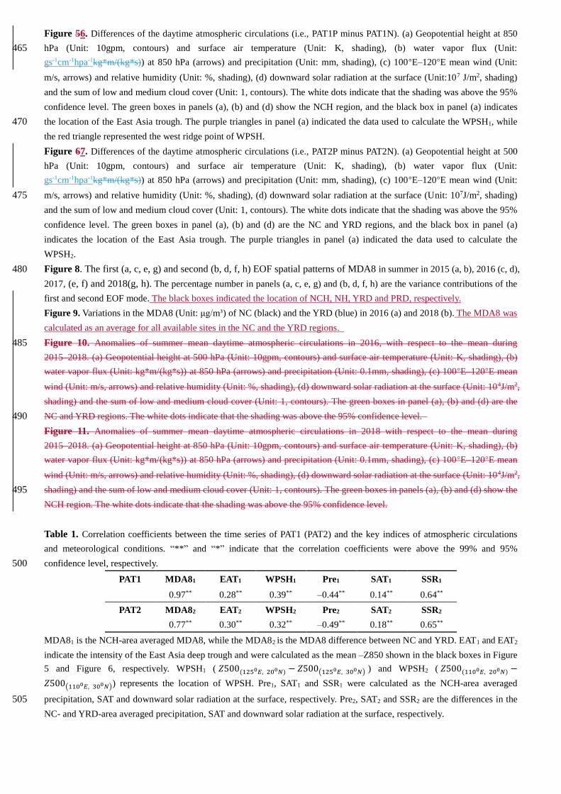
Figure 56. Differences of the daytime atmospheric circulations (i.e., PAT1P minus PAT1N). (a) Geopotential height at 850
hPa (Unit: 10gpm, contours) and surface air temperature (Unit: K, shading), (b) water vapor flux (Unit: 465
gs-1cm-1hpa-1kg*m/(kg*s)) at 850 hPa (arrows) and precipitation (Unit: mm, shading), (c) 100°E–120°E mean wind (Unit:
m/s, arrows) and relative humidity (Unit: %, shading), (d) downward solar radiation at the surface (Unit:107 J/m2, shading)
and the sum of low and medium cloud cover (Unit: 1, contours). The white dots indicate that the shading was above the 95%
confidence level. The green boxes in panels (a), (b) and (d) show the NCH region, and the black box in panel (a) indicates
the location of the East Asia trough. The purple triangles in panel (a) indicated the data used to calculate the WPSH1, while 470
the red triangle represented the west ridge point of WPSH.
Figure 67. Differences of the daytime atmospheric circulations (i.e., PAT2P minus PAT2N). (a) Geopotential height at 500
hPa (Unit: 10gpm, contours) and surface air temperature (Unit: K, shading), (b) water vapor flux (Unit:
gs-1cm-1hpa-1kg*m/(kg*s)) at 850 hPa (arrows) and precipitation (Unit: mm, shading), (c) 100°E–120°E mean wind (Unit:
m/s, arrows) and relative humidity (Unit: %, shading), (d) downward solar radiation at the surface (Unit: 107J/m2, shading) 475
and the sum of low and medium cloud cover (Unit: 1, contours). The white dots indicate that the shading was above the 95%
confidence level. The green boxes in panel (a), (b) and (d) are the NC and YRD regions, and the black box in panel (a)
indicates the location of the East Asia trough. The purple triangles in panel (a) indicated the data used to calculate the
WPSH2.
Figure 8. The first (a, c, e, g) and second (b, d, f, h) EOF spatial patterns of MDA8 in summer in 2015 (a, b), 2016 (c, d), 480
2017, (e, f) and 2018(g, h). The percentage number in panels (a, c, e, g) and (b, d, f, h) are the variance contributions of the
first and second EOF mode. The black boxes indicated the location of NCH, NH, YRD and PRD, respectively.
Figure 9. Variations in the MDA8 (Unit: μg/m³) of NC (black) and the YRD (blue) in 2016 (a) and 2018 (b). The MDA8 was
calculated as an average for all available sites in the NC and the YRD regions.
Figure 10. Anomalies of summer mean daytime atmospheric circulations in 2016, with respect to the mean during 485
2015–2018. (a) Geopotential height at 500 hPa (Unit: 10gpm, contours) and surface air temperature (Unit: K, shading), (b)
water vapor flux (Unit: kg*m/(kg*s)) at 850 hPa (arrows) and precipitation (Unit: 0.1mm, shading), (c) 100°E–120°E mean
wind (Unit: m/s, arrows) and relative humidity (Unit: %, shading), (d) downward solar radiation at the surface (Unit: 104J/m2,
shading) and the sum of low and medium cloud cover (Unit: 1, contours). The green boxes in panel (a), (b) and (d) are the
NC and YRD regions. The white dots indicate that the shading was above the 95% confidence level. 490
Figure 11. Anomalies of summer mean daytime atmospheric circulations in 2018 with respect to the mean during
2015–2018. (a) Geopotential height at 850 hPa (Unit: 10gpm, contours) and surface air temperature (Unit: K, shading), (b)
water vapor flux (Unit: kg*m/(kg*s)) at 850 hPa (arrows) and precipitation (Unit: 0.1mm, shading), (c) 100°E–120°E mean
wind (Unit: m/s, arrows) and relative humidity (Unit: %, shading), (d) downward solar radiation at the surface (Unit: 104J/m2,
shading) and the sum of low and medium cloud cover (Unit: 1, contours). The green boxes in panels (a), (b) and (d) show the 495
NCH region. The white dots indicate that the shading was above the 95% confidence level.
Table 1. Correlation coefficients between the time series of PAT1 (PAT2) and the key indices of atmospheric circulations
and meteorological conditions. “**” and “*” indicate that the correlation coefficients were above the 99% and 95%
confidence level, respectively. 500
PAT1 MDA81 EAT1 WPSH1 Pre1 SAT1 SSR1
0.97** 0.28** 0.39** –0.44** 0.14** 0.64**
PAT2 MDA82 EAT2 WPSH2 Pre2 SAT2 SSR2
0.77** 0.30** 0.32** –0.49** 0.18** 0.65**
MDA81 is the NCH-area averaged MDA8, while the MDA82 is the MDA8 difference between NC and YRD. EAT1 and EAT2
indicate the intensity of the East Asia deep trough and were calculated as the mean –Z850 shown in the black boxes in Figure
5 and Figure 6, respectively. WPSH1 ( 𝑍500(1250𝐸, 200𝑁) − 𝑍500(1250𝐸, 300𝑁) ) and WPSH2 ( 𝑍500(1100𝐸, 200𝑁) −
𝑍500(1100𝐸, 300𝑁)) represents the location of WPSH. Pre1, SAT1 and SSR1 were calculated as the NCH-area averaged
precipitation, SAT and downward solar radiation at the surface, respectively. Pre2, SAT2 and SSR2 are the differences in the 505
NC- and YRD-area averaged precipitation, SAT and downward solar radiation at the surface, respectively.

510
Figure 1. Distribution of the (a) mean values and (b) maximum values of MDA8 (Unit: μg/m³) at the observation sites in
summer from 2015 to 2018. The black boxes in panels a and b indicated the locations of North China and Huanghuai region
(NCH), North China (NC), Yangtze River Delta (YRD) and Pearl River Delta (PRD).
515


Figure 72. Anomalies of the summer mean MDA8 (Unit: μg/m³) in 2015 (a), 2016 (b), 2017 (c) and 2018 (d), relative to the
mean during 2015–2018. The black pluses indicate that the maximum MDA8 was larger than 265 μg/m³. The black boxes in 520
panel b indicated the locations of NC, YRD and PRD, while that in panel d was the NCH area.

Figure 23. Variations in MDA8 (Unit: μg/m³) of polluted cities from 2015 to 2018, including (a) Beijing (capital of China),
Tianjin and Tangshan near the capital city; (b) Taiyuan, Weifang and Shijiazhuang in the south of NCH; (c) Shanghai and 525
Nanjing in YRD; and (d) Zhongshan and Guangzhou in PRD. The cities in panels (a)-(d) were located from north to south
and were illustrated in Figure S2. The horizontal dash lines indicated the value of 100 μg/m³ and 215 μg/m³.
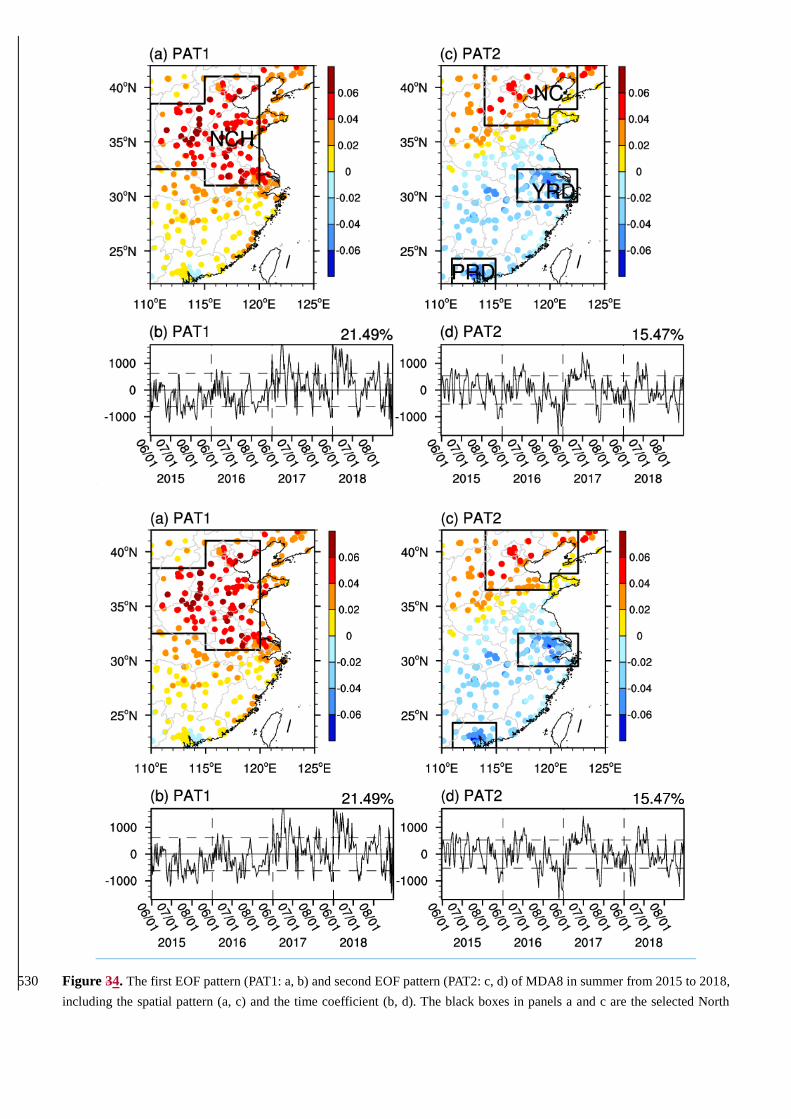
Figure 34. The first EOF pattern (PAT1: a, b) and second EOF pattern (PAT2: c, d) of MDA8 in summer from 2015 to 2018, 530
including the spatial pattern (a, c) and the time coefficient (b, d). The black boxes in panels a and c are the selected North
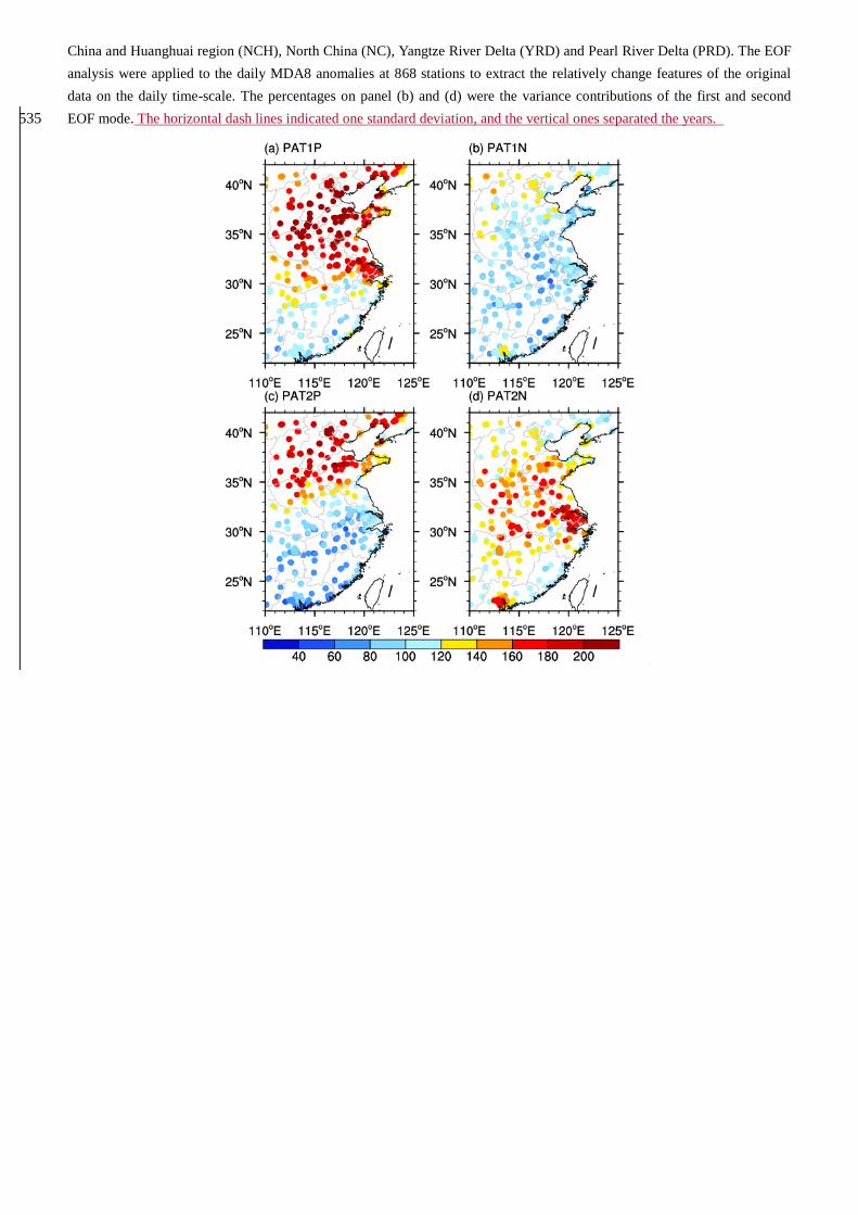
China and Huanghuai region (NCH), North China (NC), Yangtze River Delta (YRD) and Pearl River Delta (PRD). The EOF
analysis were applied to the daily MDA8 anomalies at 868 stations to extract the relatively change features of the original
data on the daily time-scale. The percentages on panel (b) and (d) were the variance contributions of the first and second
EOF mode. The horizontal dash lines indicated one standard deviation, and the vertical ones separated the years. 535

Figure 45. Composites of the MDA8 (Unit: μg/m³) for PAT1 (a, b) and PAT2 (c, d) in summer from 2015 to 2018. Panels (a)
and (c) were composited when the time coefficient of EOF1 and EOF2 was greater than one standard deviation, while panels
(b) and (d) were composited when the time coefficient was less than –﹣1×one standard deviation. The black box in panel 540
a-b indicated the location of NCH, while those in panel c-d were the NH, YRD and PRD area.
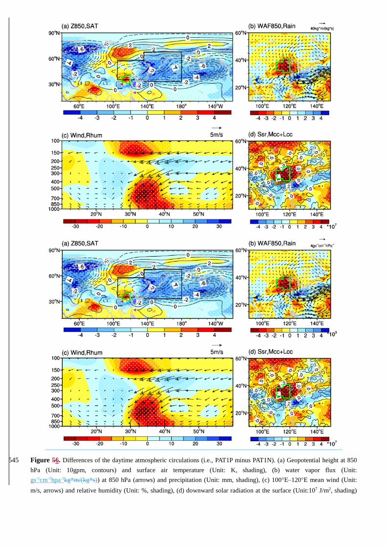
Figure 56. Differences of the daytime atmospheric circulations (i.e., PAT1P minus PAT1N). (a) Geopotential height at 850 545
hPa (Unit: 10gpm, contours) and surface air temperature (Unit: K, shading), (b) water vapor flux (Unit:
gs-1cm-1hpa-1kg*m/(kg*s)) at 850 hPa (arrows) and precipitation (Unit: mm, shading), (c) 100°E–120°E mean wind (Unit:
m/s, arrows) and relative humidity (Unit: %, shading), (d) downward solar radiation at the surface (Unit:107 J/m2, shading)

and the sum of low and medium cloud cover (Unit: 1, contours). The white dots indicate that the shading was above the 95%
confidence level. The green boxes in panels (a), (b) and (d) show the NCH region, and the black box in panel (a) indicates 550
the location of the East Asia trough. The purple triangles in panel (a) indicated the data used to calculate the WPSH1, while
the red triangle represented the west ridge point of WPSH.
555
560

Figure 67. Differences of the daytime atmospheric circulations (i.e., PAT2P minus PAT2N). (a) Geopotential height at 500
hPa (Unit: 10gpm, contours) and surface air temperature (Unit: K, shading), (b) water vapor flux (Unit:
gs-1cm-1hpa-1kg*m/(kg*s)) at 850 hPa (arrows) and precipitation (Unit: mm, shading), (c) 100°E–120°E mean wind (Unit: 565
m/s, arrows) and relative humidity (Unit: %, shading), (d) downward solar radiation at the surface (Unit: 107J/m2, shading)
and the sum of low and medium cloud cover (Unit: 1, contours). The white dots indicate that the shading was above the 95%
confidence level. The green boxes in panel (a), (b) and (d) are the NC and YRD regions, and the black box in panel (a)
indicates the location of the East Asia trough. The purple triangles in panel (a) indicated the data used to calculate the
WPSH2. 570
575
580
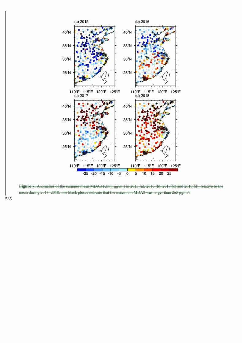
Figure 7. Anomalies of the summer mean MDA8 (Unit: μg/m³) in 2015 (a), 2016 (b), 2017 (c) and 2018 (d), relative to the
mean during 2015–2018. The black pluses indicate that the maximum MDA8 was larger than 265 μg/m³.
585


Figure 8. The first (a, c, e, g) and second (b, d, f, h) EOF spatial patterns of MDA8 in summer in 2015 (a, b), 2016 (c, d),
2017, (e, f) and 2018(g, h). The percentage number in panels (a, c, e, g) and (b, d, f, h) are the variance contributions of the 590
first and second EOF mode. The black boxes indicated the location of NCH, NH, YRD and PRD, respectively.

Figure 9. Variations in the MDA8 (Unit: μg/m³) of NC (black) and the YRD (blue) in 2016 (a) and 2018 (b). The MDA8 was 595
calculated as an average for all available sites in the NC and the YRD regions.
Figure 10. Anomalies of summer mean daytime atmospheric circulations in 2016, with respect to the mean during
2015–2018. (a) Geopotential height at 500 hPa (Unit: 10gpm, contours) and surface air temperature (Unit: K, shading), (b)
water vapor flux (Unit: kg*m/(kg*s)) at 850 hPa (arrows) and precipitation (Unit: 0.1mm, shading), (c) 100°E–120°E mean 600
wind (Unit: m/s, arrows) and relative humidity (Unit: %, shading), (d) downward solar radiation at the surface (Unit: 104J/m2,

shading) and the sum of low and medium cloud cover (Unit: 1, contours). The green boxes in panel (a), (b) and (d) are the
NC and YRD regions. The white dots indicate that the shading was above the 95% confidence level.
605
Figure 11. Anomalies of summer mean daytime atmospheric circulations in 2018 with respect to the mean during
2015–2018. (a) Geopotential height at 850 hPa (Unit: 10gpm, contours) and surface air temperature (Unit: K, shading), (b)
water vapor flux (Unit: kg*m/(kg*s)) at 850 hPa (arrows) and precipitation (Unit: 0.1mm, shading), (c) 100°E–120°E mean
wind (Unit: m/s, arrows) and relative humidity (Unit: %, shading), (d) downward solar radiation at the surface (Unit: 104J/m2,
shading) and the sum of low and medium cloud cover (Unit: 1, contours). The green boxes in panels (a), (b) and (d) show the 610
NCH region. The white dots indicate that the shading was above the 95% confidence level.
Top Related