


Languages
Pages
Legal


Reservoir Operation by Ant Colony Optimization Algorithms 1
Reservoir Operation by Ant Colony Optimization Algorithms
M. R. Jalali1; A. Afshar2; and M. A. Mariño, Hon.M.ASCE3
Abstract: In this paper, ant colony optimization (ACO) algorithms are
proposed for reservoir operation. Through a collection of cooperative agents
called ants, the near-optimum solution to the reservoir operation can be
effectively achieved. To apply ACO algorithms, the problem is approached by
considering a finite horizon with a time series of inflow, classifying the
reservoir volume to several intervals, and deciding for releases at each period
with respect to a predefined optimality criterion. Three alternative
formulations of ACO algorithms for reservoir operation are presented using a
single reservoir, deterministic, finite-horizon problem and applied to the Dez
reservoir in Iran. It is concluded that the ant colony system global-best
algorithm provides better and comparable results with known global optimum
results. Application of the model to a two-reservoir problem reveals its
potential for being extended to multi-reservoir problems. As any direct search
method, the model is quite sensitive to setup parameters, hence fine tuning of
the parameters is recommended.
Key words: Ant colony; Optimization; Reservoir operation
1Research Assistant, Iran University of Science and Technology (IUST), Tehran, Iran. E-mail: [email protected] 2 Professor, Dept. of Civil Engrg., Iran University of Science and Technology, Tehran, Iran. E-mail: [email protected] 3 Professor, Hydrology Program and Dept. of Civil and Environmental Engrg., University of Calif., Davis, CA 95616. E-mail: [email protected]

Reservoir Operation by Ant Colony Optimization Algorithms 2
Introduction
Ant colony optimization (ACO), called ant system (Colorni et al. 1991; Dorigo 1992),
was inspired by studies of the behavior of ants (Deneubourg et al. 1983). Ant algorithms
were first proposed by Dorigo (1992) and Dorigo et al. (1996) as a multi-agent approach
to different combinatorial optimization problems like the traveling salesman problem and
the quadratic assignment problem. The ant-colony metaheuristic framework was
introduced by Dorigo and Di Caro (1999), which enabled ACO to be applied to a range
of combinatorial optimization problems. Dorigo et al. (2000) also reported the successful
application of ACO algorithms to a number of bench-mark combinatorial optimization
problems.
So far, very few applications of ACO algorithms to water resources problems have been
reported (Abbaspour et al. 2001; Maier et al. 2003). Abbaspour et al. (2001) employed
ACO algorithms to estimate hydraulic parameters of unsaturated soil. Maier et al. (2003)
used ACO algorithms to find a near global optimal solution to a water distribution
system, indicating that ACO algorithms may form an attractive alternative to genetic
algorithms for the optimum design of water distribution systems.
In this paper, we propose a novel way of addressing the optimum reservoir operation
problem making use of ACO algorithms. To do so, the reservoir operation will be
structured to fit an ACO model and the features related to ACO algorithms (such as
heuristic information, pheromone trails, problem specific formulation, and pheromone
update) will be introduced. Performance of three different ACO algorithms in the
operation of the Dez reservoir in Iran, as well as the influence of the parameter settings

Reservoir Operation by Ant Colony Optimization Algorithms 3
on a final selected ACO algorithm, will be compared. The model will also be applied to
the operation of a two-reservoir system.
Ant Colony Behavior
Ant colony algorithms have been founded on the observation of real ant colonies. By
living in colonies, ants’ social behavior is directed more to the survival of the colony
entity than to that of a single individual member of the colony. An interesting and
significantly important behavior of ant colonies is their foraging behavior, and in
particular, their ability to find the shortest route between their nest and a food source,
realizing that they are almost blind. The path taken by individual ants from the nest, in
search for a food source, is essentially random (Dorigo et al. 1996). However, when they
are traveling, ants deposit on the ground a substance called pheromone, forming a
pheromone trail as an indirect communication means. By smelling the pheromone, there
is a higher probability that the trail with a higher pheromone concentration will be
chosen. The pheromone trail allows ants to find their way back to the food source and
vice versa. The trail is used by other ants to find the location of the food source located
by their nest mates. It follows that when a number of paths is available from the nest to a
food source, a colony of ants may be able to exploit the pheromone trail left by the
individual members of the colony to discover the shortest path from the nest to the food
source and back (Dorigo and Di Caro 1999). As more ants choose a path to follow, the
pheromone on the path builds up, making it more attractive to other ants seeking food and
hence more likely to be followed by other ants.

Reservoir Operation by Ant Colony Optimization Algorithms 4
As an example (Fig. 1), if an obstacle is placed on an established path leading to a food
source, ants may initially go right or left in a seemingly random manner. However, those
choosing the shortest side will reach the food more quickly and will make the return
journey more often. The pheromone on the shorter path will build up and more strongly
reinforced, and will eventually become the preferred route for the stream of ants.
Generally speaking, evolutionary algorithms search for a global optimum by generating a
population of trial solutions. Ant colony optimization, as an evolutionary algorithm, has
many features which are similar to genetic algorithms (GAs). Table 1 compares some
common and/or similar features of ACO algorithms with those of GAs, as described in
detail by Maier et al. (2003).
The most important difference between GAs and ACO algorithms is the way the trial
solutions are generated. In ACO algorithms, trial solutions are constructed incrementally
based on the information contained in the environment and the solutions are improved by
modifying the environment via a form of indirect communication called stigmergy
(Dorigo et al. 2000). On the other hand, in GAs the trial solutions are in the form of
strings of genetic materials and new solutions are obtained through the modification of
previous solutions (Maier et al. 2003). Thus, in GAs the memory of the system is
embedded in the trial solutions, whereas in ACO algorithms the system memory is
contained in the environment itself.
Ant Colony Optimization (ACO) Algorithms: General Aspects
In general, ACO algorithms employ a finite size of artificial agents with defined
characteristics which collectively search for good quality solutions to the problem under

Reservoir Operation by Ant Colony Optimization Algorithms 5
consideration. Starting from an initial state selected according to some case-dependent
criteria, each ant builds a solution which is similar to a chromosome in a genetic
algorithm. While building its own solution, each ant collects information on its own
performance and uses this information to modify the representation of the problem, as
seen by the other ants (Dorigo and Gambardella 1997). The ant's internal states store
information about the ant’s past behavior, which can be employed to compute the
goodness/value of the generated solution. In many optimization problems, some paths
available to an ant in a given state may lead the ant to an infeasible state, which can be
avoided using the ant's memory. Artificial ants are permitted to release pheromone while
developing a solution or after a solution has fully been developed, or both. The amount of
pheromone deposited is made proportional to the goodness of the solution an artificial ant
has developed (or is developing).
Rapid drift of all the ants towards the same part of the search space is avoided by
employing the stochastic component of the choice decision policy and the pheromone
evaporation mechanism. To simulate pheromone evaporation, the pheromone persistence
coefficient (ρ) is defined which enables greater exploration of the search space and
minimizes the chance of premature convergence to suboptimal solutions (see Eq. 4). A
probabilistic decision policy is also used by the ants to direct their search towards the
most interesting regions of the search space. The level of stochasticity in the policy and
the strength of the updates in the pheromone trail determine the balance between the
exploration of new points in the state space and the exploitation of accumulated
knowledge (Dorigo and Gambardella 1997). Once an ant has fulfilled its task and upon

Reservoir Operation by Ant Colony Optimization Algorithms 6
deposition of pheromone information, it "dies." In other words, it will be deleted from the
system.
Let τij(t) be the total pheromone deposited on path ij at time t, and ηij(t) be the heuristic
value of path ij at time t according to the measure of the objective function. We define the
transition probability from node i to node j at time period t as:
[ ] [ ][ ] [ ]
∈
ητ
ητ
= ∑∈
βα
βα
otherwise 0
allowedj if )t()t(
)t()t(
)t(Pallowedl
ilil
ijij
ij (1)
where α and β = parameters that control the relative importance of the pheromone trail
versus a heuristic value.
Let q be a random variable uniformly distributed over [0, 1], and q0 ∈ [0, 1] be a tunable
parameter. The next node j that ant k chooses to go is:
[ ] [ ]{ }
≤
= ∈
otherwiseJ
qqifttj ililallowedl k
)()(max arg 0βα ητ
(2)
where J = a random variable selected according to the probability distribution of Pij(t).
The pheromone trail is changed both locally and globally. Local updating is intended to
avoid a very strong path being chosen by all the ants. Every time a path is chosen by an
ant, the amount of pheromone will change by applying the local trail updating formula:
0).1()(.)( τδτδτ −+← tt ijstep
ij (3)

Reservoir Operation by Ant Colony Optimization Algorithms 7
where 0τ = initial value of pheromone; δ = tuning parameter ( 10 ≤≤ δ ); and the symbol
←step is used to show the next step. Upon completion of a tour by all ants in the
colony, the global trail updating is done as follows:
ijijiteration
ij tt τρτρτ ∆−+ ← ).1()(.)( (4)
where 0 ≤ ρ ≤ 1; (1 - ρ) = evaporation (i.e., loss) rate; and the symbol ←iteration is
used to show the next iteration.
There are several definitions for )(tijτ∆ (Dorigo et al. 1996; Dorigo and
Gambardella 1997). In this paper, we use three algorithms as:
1. Ant System (AS) algorithm
∑=
=∆M
k
kijij tmt
1)()( ττ (5)
∉
∈=
)(),( 0)(),( )(/1
)(mTjiifmTjiifmG
tmk
kkkijτ (6)
where Gk(m) = value of the objective function for the tour Tk(m) taken by the k-th ant at
iteration m.
2. Ant Colony System–Iteration Best (ACSib)

Reservoir Operation by Ant Colony Optimization Algorithms 8
∈
=∆otherwise 0
ant by done tour ),( )(/1)( ib
k
ijkjiifmG
tib
τ (7)
where )(mG ibk = value of the objective function for the ant taken the best tour at iteration
m.
3. Ant Colony System–Global Best (ACSgb)
∈
=∆otherwise 0
ant by done tour ),( /1)( gb
k
ijkjiifG
tgb
τ (8)
where gbkG = value of the objective function for the ant with the best performance within
the past total iteration.
ACO Algorithms for Optimum Reservoir Operation
To apply ACO algorithms to a specific problem, the following steps have to be taken: (1)
Problem representation as a graph or a similar structure easily covered by ants; (2)
Assigning a heuristic preference to generated solutions at each time step (i.e., selected
path by the ants); (3) Defining a fitness function to be optimized; and (4) Selection of an
ACO algorithm to be applied to the problem. In the following subsections, these steps
will be introduced to solve the optimum reservoir operation problem.
Problem representation

Reservoir Operation by Ant Colony Optimization Algorithms 9
To apply ACO algorithms to the optimum reservoir operation problem, it is convenient to
see it as a combinatorial optimization problem with the capability of being represented as
a graph. The problem may be approached considering a time series of inflow, classifying
the reservoir volume to several intervals, and deciding for releases at each period with
respect to an optimality criterion. Links between initial and final storage volumes at
different periods form a graph which represents the system, determining the release at
that period (Fig. 2).
Heuristic information
The heuristic information on this problem is determined by considering the criterion as
minimum deficit:
[ ] ))()(/(1)( 2 ctDtRt ijij +−=η (9)
where Rij(t) = release at period t, provided the initial and final storage volume at classes i
and j, respectively; D(t) = demand of period t; and c = a constant to avoid irregularity
(dividing by zero in Eq. 9.). To determine Rij(t), the continuity equation along with the
following constraints, may be employed as:
)()()( tLOSStISStR ijjiij −+−= (10a)
maxmin SSS i ≤≤ (10b)
maxmin SSS j ≤≤ (10c)
11 += NTSS (10d)

Reservoir Operation by Ant Colony Optimization Algorithms 10
where Si and Sj = initial and final storage volumes (class i and j), respectively; I(t) =
inflow to the reservoir at time period t; LOSSij(t) = loss (e.g., evaporation) at period t
provided that initial and final storage at classes i and j respectively; Smin and Smax =
minimum and maximum storage allowed respectively; and NT= total number of periods.
Using the transition rule (Eq. 2), each ant is free to choose the class of final storage (end-
of-period storage), if it is feasible through the continuity equation and storage constraints
(Eqs. 10).
Fitness function
The fitness function is a measure of the goodness of the generated solutions according to
the defined objective function. For this study, total square deviation (TSD) is defined as:
[ ]∑=
−=NT
t
kk tDtRTSD1
2)()( (11)
where Rk(t) = release at period t recommended by ant k.
ACO algorithms
Three different ACO algorithms, namely: the Ant System (AS), the Ant Colony System–
Iteration Best (ACSib), and the Ant Colony System–Global Best (ACSgb), have been
tested. The so-called solution construction and pheromone trail update rule considered by
these ACO algorithms are employed. Due to the special structure of the model, the local
update rule is disregarded. In fact, the random distribution of ants in different classes of
discretized storage volumes as well as along the 60-month operation horizon makes the
local update rule inefficient. In reservoir operation problem, the local update rule is

Reservoir Operation by Ant Colony Optimization Algorithms 11
strongly recommended if a single starting point for all agents (i.e., same initial storage
volume and time period) is chosen.
Model Application
To illustrate the performance of the model, the Dez reservoir in southern Iran, with an
effective storage volume of 2,510 MCM and average annual demand of 5,900 MCM is
selected. For illustration purposes, a period of 60 months with an average annual inflow
of 5,303 MCM is employed. The reservoir volume is divided into 14 classes with 200
MCM intervals. To limit the range of values of the fitness function, a normalized form of
Eq. 11 has been used as:
[ ]∑=
−=NT
t
kk DtDtRTSD1
2max/))()(( (12)
where Dmax = maximum monthly demand.
To start with the model, a finite number of ants is randomly distributed in different
classes of initial storage volume. It is also assumed that the starting point for ants could
be any time along the 60-month operation horizon. Thus, ants are also uniformly random
distributed along the operation horizon (Fig. 2). Feasible paths for ants to follow are
constrained by the continuity equation, and the minimum and maximum permitted
storage volume (Eqs. 10). By completion of the first tour by all ants, there will be a finite
number of feasible solutions with values for the objective function. Now, realizing the
values of the fitness function, the pheromones must be updated to continue the next
iteration. To update the pheromones, three previously defined ACO algorithms are

Reservoir Operation by Ant Colony Optimization Algorithms 12
employed (Eqs. 5-8). When the pheromone update is completed, the next iteration begins.
A simple flow diagram of ACO algorithms for the optimum reservoir operation is
depicted in Fig. 3.
To compare the performance of different ACO algorithms for updating pheromones in
reservoir operation, three well-known systems, namely (1) Ant System (AS); (2) Ant
Colony System with iteration-best (ACSib); and (3) Ant Colony System with global-best
(ACSgb) will be used. The main difference between them is due to global pheromone
updating procedures. In the AS algorithm, pheromone updating may be accomplished
using all ants upon a tour completion. However, in ACSib the ant with the best result in
each iteration, will be employed for pheromone updating. On the other hand in ACSgb,
the pheromone updating may be left to the ant with the best performance within the past
total iterations.
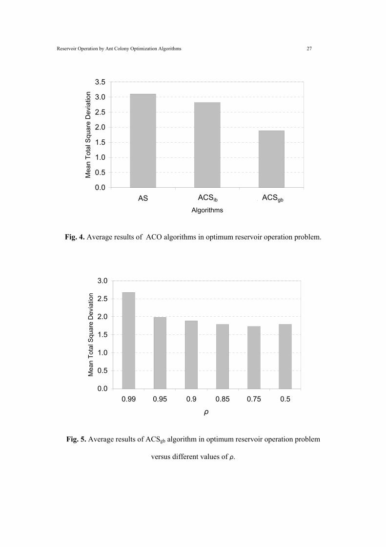
The model so developed was tested for the Dez reservoir with 10 runs. Results of the
model are presented in Table 2 and Fig. 4. The total number of ants (M) assigned to the
problem was 30, with ρ= 0.9, α = 1, β = 2, and q0 = 0.9. To start with, the pheromone was
uniformly distributed all over the defined paths (i.e., 10 =τ ). To normalize the value of
the heuristic function, the parameter c was chosen to be unity (Eq. 9). The total number
of iterations at each run was limited to 200.
Referring to Table 2 and Fig. 4, ACS algorithms provide better results compared to the
AS algorithm. In general, the ACSgb reveals a much better performance, with almost 39
and 33 percent improvement compared to AS and ACSib , respectively.
As with any search method, the performance of the ACSgb algorithm in reservoir
operation depends on the model parameters. For a given problem, with NT = 60 months,
Reservoir Operation by Ant Colony Optimization Algorithms 13
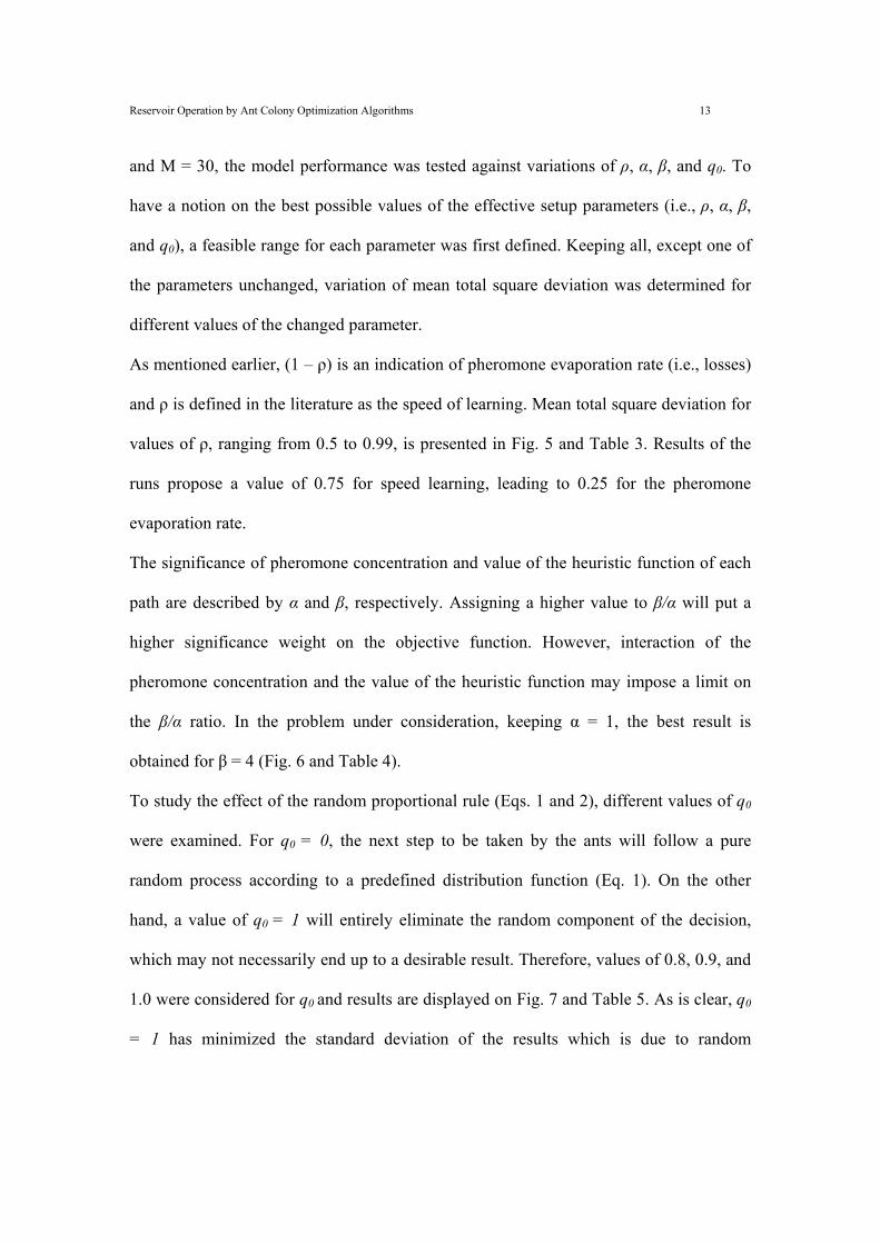
and M = 30, the model performance was tested against variations of ρ, α, β, and q0. To
have a notion on the best possible values of the effective setup parameters (i.e., ρ, α, β,
and q0), a feasible range for each parameter was first defined. Keeping all, except one of
the parameters unchanged, variation of mean total square deviation was determined for
different values of the changed parameter.
As mentioned earlier, (1 – ρ) is an indication of pheromone evaporation rate (i.e., losses)
and ρ is defined in the literature as the speed of learning. Mean total square deviation for
values of ρ, ranging from 0.5 to 0.99, is presented in Fig. 5 and Table 3. Results of the
runs propose a value of 0.75 for speed learning, leading to 0.25 for the pheromone
evaporation rate.
The significance of pheromone concentration and value of the heuristic function of each
path are described by α and β, respectively. Assigning a higher value to β/α will put a
higher significance weight on the objective function. However, interaction of the
pheromone concentration and the value of the heuristic function may impose a limit on
the β/α ratio. In the problem under consideration, keeping α = 1, the best result is
obtained for β = 4 (Fig. 6 and Table 4).
To study the effect of the random proportional rule (Eqs. 1 and 2), different values of q0
were examined. For q0 = 0, the next step to be taken by the ants will follow a pure
random process according to a predefined distribution function (Eq. 1). On the other
hand, a value of q0 = 1 will entirely eliminate the random component of the decision,
which may not necessarily end up to a desirable result. Therefore, values of 0.8, 0.9, and
1.0 were considered for q0 and results are displayed on Fig. 7 and Table 5. As is clear, q0
= 1 has minimized the standard deviation of the results which is due to random
Reservoir Operation by Ant Colony Optimization Algorithms 14
component elimination. A value of 0.9 for q0 seems to be the best choice for the problem
under consideration resulting in a mean total square deviation of 1.62 units.
The effect of the number of iterations and number of ants on mean total square deviation
was examined using 50 to 500 iterations and 20 to 100 ants. Results are depicted in Table
6 and Figs. 8 and 9. As expected, the results improve as the number of iterations and
number of ants increase. However, there seems to be a trade-off between the number of
iterations and the total number of ants initially distributed. The best result was observed
with 500 iterations and 100 ants, leading to the best total square deviation of 1.296 units.
It needs to be mentioned that the best result was obtained for ρ= 0.75, α = 1, β = 4, and q0
= 0.9, which resulted from parameter-tuning.
The best overall result obtained from ACSgb for initial and final storage volumes of 1,430
MCM is 1.296 (TSD). The global optimum with the same initial and final storage
volumes resulted in TSD = 1.273. Clearly, the developed model with the ACSgb
algorithm for pheromone updating provides comparable results with those of global
optimum, and seems promising in optimum reservoir operation. The fluctuation of
volume and reservoir release, taken from two models is presented in Figs. 10 and 11.
Except for a few months, reservoir releases and storage volumes resulting from the
proposed algorithm follow those of global optimum very well.
Application to a Two-Reservoir Problem
To test the application of ACO algorithms to a multiple reservoir system, a hypothetical
system with two reservoirs was considered (Fig. 12). Active storage capacities of 1,720
MCM and 2,510 MCM are considered for upstream and downstream reservoirs,

Reservoir Operation by Ant Colony Optimization Algorithms 15
respectively. Annual demand of 3,930 MCM and 5,900 MCM with the same monthly
pattern are assigned for Reservoirs 1 and 2, respectively. Monthly distribution of annual
inflow to reservoirs is kept the same as for the single reservoir problem. Total annual
inflow to Reservoirs 1 and 2 is assumed to be 8,635 MCM and 5,757 MCM, respectively.
A new fitness function is defined for the two-reservoir system:
{ [ ] [ ] }∑=
−+−=NT
tdd
kduu
ku
k DtDtRDtDtRTSD1
2max,
2max, /))()((/))()(( (13)
where subscripts u and d refer to upstream and downstream reservoirs, respectively. To
run the model, storage volume in Reservoir 1 was discretized into 10 classes with 200
MCM intervals and that of Reservoir 2 was discretized into 14 classes with the same
intervals. A total number of 20 ants was assigned with 100 iterations, where the tuning
parameter was taken from the single reservoir problem (i.e., ρ = 0.75, α = 1, β = 4, and q0
= 0.9). Results of 10 runs for a 12-month period is presented in Table 7, with TSD =
18.372 being the best out of 10 runs. In this case, Reservoirs 1 and 2 start with initial
storages of 520 MCM and 830 MCM, respectively.
As mentioned earlier, in ACO algorithms the information is contained in the environment
and is used to construct the new improved trial solution by modifying the environment.
Hence, information regarding the pheromone intensities must be saved which may call
for a higher computer memory. Development of a pheromone allocation algorithm to
save the computer memory and application of ACO algorithms to multiple reservoirs is
currently being studied.

Reservoir Operation by Ant Colony Optimization Algorithms 16
Concluding Remarks
While walking from one point to another, ants deposit a substance called pheromone,
forming a pheromone trail. It has been shown experimentally (Dorigo et al. 1996) that
this pheromone trail, once employed by a colony of ants, can give rise to the emergence
of a shortest path. In general, the amount of pheromone deposited is made proportional to
the goodness of the solution an ant may build. To apply ACO algorithms to the reservoir
operation problem, one may view it as a combinatorial optimization problem. The
problem may be approached by considering a time series of inflow, classifying the
reservoir volume to several intervals, and deciding on the release at each period with
respect to an optimality criterion. Feasible paths for ants to follow may be constrained by
the continuity equation as well as constraints on the storage volume. Upon each tour
completion, a finite number of feasible solutions will form, leaving a new value for the
pheromone.
Realizing the values of the fitness function, the pheromones will be updated by global
and local update rules. Application of the proposed model to the Dez reservoir in Iran
provided promising results. From three different pheromone updating algorithms (i.e.,
Ant System, Ant Colony System-iteration best, Ant Colony System-global best), the
ACSgb provides better and comparable results with those of global optimum in optimum
reservoir operation. Application of the model to a two-reservoir problem reveals its
potential for being extended to multi-reservoir problems. As for any search method, the
performance of the proposed model is quite sensitive to setup parameters, hence fine
tuning of the parameters is recommended.

Reservoir Operation by Ant Colony Optimization Algorithms 17
References
Abbaspour, K. C., Schulin, R., and van Genuchten, M. T. (2001). "Estimating unsaturated
soil hydraulic parameters using ant colony optimization." Adv. Water Resour., 24(8),
827-933.
Colorni, A., Dorigo, M., and Maniezzo, V. (1991). "Distributed optimization by ant-
colonies" Proc., 1st European Conf. on Artificial Life (ECAL'91), Cambridge, Mass,
USA, MIT Press, 134-142.
Deneubourg, J. L., Pasteels, J. M., Verhaeghe, J. C. (1983). "Probabilistic behavior in
ants: A strategy of errors?" J. Theoretical Biology, 105, 259-271.
Dorigo, M. (1992). "Optimization, learning and natural algorithms" Ph.D. Thesis,
Politecnico di Milano, Italy.
Dorigo, M., Maniezzo, V., and Colorni, A. (1996). "The ant system: optimization by a
colony of cooperating ants." IEEE Trans. Syst. Man. Cybern., 26, 29-42.
Dorigo, M., and Gambardella, L. M. (1997). "Ant colony system: A cooperative learning
approach to the traveling salesman problem." IEEE Transactions on Evolutionary
Computation, 1(1), 53-66.
Dorigo, M., and Di Caro, G. (1999). "The ant colony optimization metaheuristic." New
ideas in optimization, D. Corne, M. Dorigo, and F. Glover, eds., McGraw-Hill, London,
11-32.
Dorigo, M., Bonabeau, E., and Theraulaz, G. (2000). "Ant algorithms and stigmergy."
Future Generation Comput. Systems, 16, 851-871.

Reservoir Operation by Ant Colony Optimization Algorithms 18
Maier, H. R., Simpson, A. R., Zecchin, A. C., Foong, W. K., Phang, K. Y., Seah, H. Y.,
and Tan, C. L. (2003). "Ant colony optimization for design of water distribution
systems." J. Water Resour. Plng. and Mgmt., 129(3), 200-209.

Reservoir Operation by Ant Colony Optimization Algorithms 19
Notations
The following symbols are used in this paper:
ρ = pheromone persistence coefficient.
Pij(t) = transition probability from node i to node j at time period t.
τij(t) = total pheromone deposited on path ij at time t.
ηij(t) = the heuristic value of path ij at time t.
α , β = parameters that control the relative importance of the pheromone trail versus a
heuristic value.
q = a random variable uniformly distributed over [0, 1].
q0 = be a tunable parameter ∈ [0, 1].
0τ = initial value of pheromone.
δ = tuning parameter ∈ [0, 1].
)(tijτ∆ = total change in pheromone of path ij at time period t.
)t(mkijτ = change in pheromone of path ij at time period t associated to ant k.
Gk(m) = value of the objective function of ant k at iteration m.
Tk(m) = the tour taken by ant k at iteration m.
)(mG ibk = value of the objective function for the ant taken the best tour at iteration m.
gbkG = value of the objective function for the ant with the best performance within
the past total iteration.
Rij(t) = release at period t.
D(t) = demand of period t.
c = a constant.
S = storage.

Reservoir Operation by Ant Colony Optimization Algorithms 20
I(t) = inflow to the reservoir at time period t.
LOSSij(t) = loss (e.g., evaporation) at period t provided that initial and final storage at
classes i and j respectively.
Smin = minimum storage allowed.
Smax = maximum storage allowed.
NT = total number of periods.
TSD = total square deviation.
Rk(t) = release at period t recommended by ant k.
Dmax = maximum monthly demand.

Reservoir Operation by Ant Colony Optimization Algorithms 21
Table 1. Similarities of ACO and genetic algorithms
Genetic Algorithm ACO Algorithm
Population size Number of ants
One generation One iteration
Trial solutions utilize the principle of survival of the fittest
It is based on foraging behavior of ant colonies
Probabilistic process is governed by crossover and mutation
Probabilistic process is defined by pheromone intensities and local heuristic information
Encouraging wider search space is achieved by mutation operator
Wider search space is guaranteed by pheromone evaporation
Table 2. Comparison of ACO algorithms in optimum reservoir operation.
* Standard deviation
** Coefficient of Variation
Algorithms Runs AS ACSib ACSgb 1 3.072 2.717 1.923 2 3.178 2.334 2.097 3 2.975 2.745 1.877 4 3.028 2.643 1.974 5 3.199 2.951 1.896 6 3.077 3.068 1.771 7 3.184 3.084 1.562 8 3.185 3.095 2.095 9 3.134 2.651 1.952 10 3.067 2.960 1.744 Mean 3.110 2.825 1.889 The Best 2.975 2.334 1.562 The Worst 3.199 3.095 2.097 S.D.* 0.077 0.248 0.163 C.V.** 0.025 0.088 0.086

Reservoir Operation by Ant Colony Optimization Algorithms 22
Table 3. Influence of parameter ρ on the results of ACSgb algorithm in optimum reservoir
operation problem.
Table 4. Influence of parameter β on the results of ACSgb algorithm in optimum reservoir
operation problem.
ρ Runs 0.99 0.95 0.90 0.85 0.75 0.50 1 2.817 2.008 1.923 1.529 1.651 1.639 2 2.205 2.240 2.097 1.837 1.788 1.835 3 2.832 2.009 1.877 1.959 1.796 1.753 4 2.408 1.829 1.974 1.693 1.893 1.693 5 2.754 1.879 1.896 2.014 1.685 1.730 6 2.669 2.038 1.771 1.668 1.746 1.761 7 2.731 2.074 1.562 1.753 1.683 1.986 8 2.864 1.869 2.095 1.916 1.770 1.838 9 2.712 2.162 1.952 1.844 1.573 1.817 10 2.783 1.737 1.744 1.682 1.716 1.859 Mean 2.678 1.985 1.889 1.790 1.730 1.791 The Best 2.205 1.737 1.562 1.529 1.573 1.639 The Worst 2.864 2.240 2.097 2.014 1.893 1.986 S.D. 0.210 0.156 0.163 0.151 0.089 0.098 C.V. 0.078 0.079 0.086 0.084 0.052 0.055
β Runs 1 2 3 4 5 1 1.756 1.651 1.848 1.489 1.557 2 1.734 1.788 1.619 1.615 1.941 3 2.038 1.796 1.661 1.537 1.675 4 1.939 1.893 1.698 1.649 1.806 5 2.007 1.685 1.843 1.642 1.514 6 2.199 1.746 1.767 1.577 1.574 7 1.981 1.683 1.702 1.791 1.564 8 1.963 1.770 1.682 1.621 1.627 9 1.853 1.573 1.657 1.751 1.626 10 1.832 1.716 1.628 1.510 1.646 Mean 1.930 1.730 1.711 1.618 1.653 The Best 1.734 1.573 1.619 1.489 1.514 The Worst 2.199 1.893 1.848 1.791 1.941 S.D. 0.141 0.089 0.082 0.098 0.130 C.V. 0.073 0.052 0.048 0.060 0.078

Reservoir Operation by Ant Colony Optimization Algorithms 23
Table 5. Influence of q0 on the results of ACSgb algorithm in optimum reservoir operation
problem.
Table 7. Results of 10 runs of two-reservoir problem.
q0 Runs 0.8 0.9 1.0 1 1.555 1.489 1.752 2 1.794 1.615 1.799 3 1.784 1.537 1.818 4 1.836 1.649 1.752 5 1.902 1.642 1.740 6 1.932 1.577 1.752 7 1.798 1.791 1.772 8 2.024 1.621 1.627 9 1.956 1.751 1.703 10 2.015 1.510 1.645 Mean 1.860 1.618 1.736 The Best 1.555 1.489 1.627 The Worst 2.024 1.791 1.818 S.D. 0.139 0.098 0.061 C.V. 0.075 0.060 0.035
Runs Total Square Deviation 1 24.072 2 24.988 3 23.614 4 18.372 5 25.526 6 24.773 7 25.922 8 26.143 9 25.803 10 26.531 Mean 24.574 The Best 18.372 The Worst 26.531 S.D. 2.366 C.V. 0.096

Reservoir Operation by Ant Colony Optimization Algorithms 24
Table 6. Influence of number of iterations and number of ants on results of ACSgb
algorithm in optimum reservoir operation problem.
Number of Iterations Number of Ants Parameters 50 100 200 300 500
20 Mean 2.293 1.960 1.690 1.653 1.527 The Best 1.959 1.777 1.547 1.519 1.317 The Worst 2.494 2.209 1.813 1.786 1.714 S.D. 0.163 0.125 0.085 0.073 0.132 C.V. 0.071 0.064 0.050 0.044 0.087
30 Mean 2.236 1.847 1.618 1.586 1.473 The Best 1.913 1.594 1.489 1.424 1.347 The Worst 2.407 2.167 1.791 1.744 1.577 S.D. 0.159 0.180 0.098 0.095 0.074 C.V. 0.071 0.097 0.060 0.060 0.051
50 Mean 2.034 1.771 1.514 1.484 1.428 The Best 1.827 1.517 1.383 1.413 1.341 The Worst 2.268 1.999 1.669 1.630 1.515 S.D. 0.137 0.172 0.090 0.074 0.055 C.V. 0.067 0.097 0.060 0.050 0.038
75 Mean 1.924 1.653 1.508 1.429 1.394 The Best 1.669 1.447 1.349 1.348 1.308 The Worst 2.421 1.884 1.647 1.576 1.540 S.D. 0.237 0.137 0.094 0.069 0.080 C.V. 0.123 0.083 0.062 0.048 0.057
100 Mean 1.948 1.650 1.457 1.404 1.417 The Best 1.795 1.467 1.325 1.322 1.296 The Worst 2.115 1.743 1.597 1.506 1.592 S.D. 0.091 0.086 0.083 0.061 0.082 C.V. 0.047 0.052 0.057 0.043 0.058

Reservoir Operation by Ant Colony Optimization Algorithms 25
(a)
(b)
(c)
(d)
Fig. 1. (a) Real ants are walking on a path between nest and food source; (b) an obstacle
suddenly appears; ants choose whether to turn left or right with equal probability; (c)
pheromone is deposited more quickly on the shorter path; and (d) all ants have chosen the
shorter path.
Fig. 2. Random distribution of ants through periods and storage volume classes at the
beginning of each iteration.
1 2 3
1
2
3
Periods
NT
NC
Vol
ume
Cla
sses

Reservoir Operation by Ant Colony Optimization Algorithms 26
Fig. 3. ACO algorithm for optimum reservoir operation.
Assign 0)( ττ =tij
Compute )(tijη according to continuity eq.
Random distribute the starting period and class of initial reservoir volume of each ant ( )(),( innins kk )
Choose the next class of reservoir volume according to state transition rule and satisfying continuity eq. ( )1( +tsk )
Compute the release ( )(tRk ) and objective value
(Squared Deviation )(tSDk )
k = No. of ants
t = NT
∑=
=NT
tkk tSDTSD
1
)( (Total Square Deviation)
Update τ values according to algorithm
End Condition
End
No
Yes
Yes
No
No
Yes
Reservoir Operation by Ant Colony Optimization Algorithms 27
0.0
0.5
1.0
1.5
2.0
2.5
3.0
3.5
AS ACS(ib) ACS(gb)Algorithms
Mea
n To
tal S
quar
e D
evia
tion
ACSib ACSgb
Fig. 4. Average results of ACO algorithms in optimum reservoir operation problem.
0.0
0.5
1.0
1.5
2.0
2.5
3.0
0.99 0.95 0.9 0.85 0.75 0.5
ρ
Mea
n To
tal S
quar
e D
evia
tion
Fig. 5. Average results of ACSgb algorithm in optimum reservoir operation problem
versus different values of ρ.

Reservoir Operation by Ant Colony Optimization Algorithms 28
1.501.551.601.651.701.751.801.851.901.952.00
1 2 3 4 5β
Mea
n To
tal S
quar
e D
evia
tion
Fig. 6. Average results of ACSgb algorithm in optimum reservoir operation problem
versus different values of β.
1.5
1.6
1.7
1.8
1.9
0.8 0.9 1
q0
Mea
n To
tal S
quar
e D
evia
tion
Fig. 7. Average results of ACSgb algorithm in optimum reservoir operation problem
versus different values of q0.

Reservoir Operation by Ant Colony Optimization Algorithms 29
No. of ants
1.2
1.4
1.6
1.8
2.0
2.2
2.4
50 100 200 300 500
No. of iterations
Mea
n To
tal S
quar
e D
evia
tion
20
30
50
75
100
Fig. 8. Mean TSD variation versus number of iterations for different numbers of ants.
No. of iterations
1.2
1.4
1.6
1.8
2.0
2.2
2.4
20 30 50 75 100No. of ants
Mea
n To
tal S
quar
e D
evia
tion
50
100
200
300
500
Fig. 9. Mean TSD variation versus number of ants for different numbers of iterations.

Reservoir Operation by Ant Colony Optimization Algorithms 30
500
1000
1500
2000
2500
3000
3500
1 5 9 13 17 21 25 29 33 37 41 45 49 53 57
Periods
Res
ervo
ir V
olum
e (M
CM
)
Global optimum ACS(gb)ACSgb
Fig. 10. Comparison of reservoir storage volume resulting from ACSgb and global
optimum.
0
100
200
300
400
500
600
700
800
900
1000
1 5 9 13 17 21 25 29 33 37 41 45 49 53 57
Periods
Rel
ease
(MC
M)
Global optimum ACS(gb)ACSgb
Fig. 11. Comparison of reservoir releases resulting from ACSgb and global optimum.

Reservoir Operation by Ant Colony Optimization Algorithms 31
Fig. 12. Configuration of two-reservoir system.
1
2
Du
Dd
Top Related