Download - Reinforcement Learning to Optimize Lifetime Value in Cold ...

Reinforcement Learning to Optimize Lifetime Value inCold-Start Recommendation

Luo JiDAMO Academy, Alibaba Group

Hangzhou, [email protected]

Qi Qin∗†Center for Data Science, AAIS, Peking University

Beijing, [email protected]

Bingqing HanDAMO Academy, Alibaba Group


Hongxia Yang‡DAMO Academy, Alibaba Group


ABSTRACTRecommender system plays a crucial role in modern E-commerceplatform. Due to the lack of historical interactions between usersand items, cold-start recommendation is a challenging problem.In order to alleviate the cold-start issue, most existing methodsintroduce content and contextual information as the auxiliary in-formation. Nevertheless, these methods assume the recommendeditems behave steadily over time, while in a typical E-commerce sce-nario, items generally have very different performances throughouttheir life period. In such a situation, it would be beneficial to con-sider the long-term return from the item perspective, which isusually ignored in conventional methods. Reinforcement learning(RL) naturally fits such a long-term optimization problem, in whichthe recommender could identify high potential items, proactivelyallocate more user impressions to boost their growth, thereforeimprove the multi-period cumulative gains. Inspired by this idea,we model the process as a Partially Observable and ControllableMarkov Decision Process (POC-MDP), and propose an actor-criticRL framework (RL-LTV) to incorporate the item lifetime values(LTV) into the recommendation. In RL-LTV, the critic studies his-torical trajectories of items and predict the future LTV of fresh item,while the actor suggests a score-based policy which maximizes thefuture LTV expectation. Scores suggested by the actor are thencombined with classical ranking scores in a dual-rank framework,therefore the recommendation is balanced with the LTV consid-eration. Our method outperforms the strong live baseline with arelative improvement of 8.67% and 18.03% on IPV and GMV ofcold-start items, on one of the largest E-commerce platform.

∗The first two authors contributed equally to this research.†This work was done when Qin Qi was an intern at Alibaba.‡Corresponding author

Permission to make digital or hard copies of all or part of this work for personal orclassroom use is granted without fee provided that copies are not made or distributedfor profit or commercial advantage and that copies bear this notice and the full citationon the first page. Copyrights for components of this work owned by others than ACMmust be honored. Abstracting with credit is permitted. To copy otherwise, or republish,to post on servers or to redistribute to lists, requires prior specific permission and/or afee. Request permissions from [email protected] ’21, November 1–5, 2021, Virtual Event, QLD, Australia© 2021 Association for Computing Machinery.ACM ISBN 978-1-4503-8446-9/21/11. . . $15.00https://doi.org/10.1145/3459637.3482292

CCS CONCEPTS• Computing methodologies → Reinforcement learning; •Information systems → Recommender systems; • Appliedcomputing→ Online shopping.

KEYWORDSCold-Start Recommendation, Reinforcement Learning, Actor-CriticModel, POC-MDP, Lifetime ValueACM Reference Format:Luo Ji, Qi Qin, Bingqing Han, and Hongxia Yang. 2021. ReinforcementLearning to Optimize Lifetime Value in Cold-Start Recommendation. InProceedings of the 30th ACM International Conference on Information andKnowledge Management (CIKM ’21), November 1–5, 2021, Virtual Event, QLD,Australia. ACM, New York, NY, USA, 10 pages. https://doi.org/10.1145/3459637.3482292

1 INTRODUCTIONRecommender systems (RS) have become increasingly popular andhave been utilized in a variety of domains (e.g. products, music,movies and etc.) [1]. RS assists users in their information seekingtasks by suggesting a list of items (i.e., products) that best fits thetarget user’s preference. For a practical system, a common pipelineis that a series of items are first retrieved from enormous candidates,then sorted by the ranking strategy to optimize some expectedmetric such as CTR (i.e., Click-Through Rate) [20].

However, due to the lack of user-item interactions, a commonchallenge is the cold-start recommendation problem [42]. Solutionto the cold-start problem may depend on the platform characteris-tics. Traditional way to solve the cold-start problem is leveragingauxiliary information into the recommendation systems (e.g., con-tent based [27, 34], heterogeneous information [25, 28] and cross-domain [19, 31]). Although they have achieved good performance,they focus on the instant reward, while the long-term rewards isignored. Correspondingly, there is recently increasing attention onthe long-term/delayed metric, and solution to optimize the long-term user engagement [35, 43] is proposed. However, a long-termviewpoint from the item aspect is still missing.

In the case of E-commerce, where the recommended items aretypically products, there is a clear need to consider their long-termbehaviors, which are changing throughout their life periods. Thelife dynamics of products share a similar development pattern, as

arX

iv:2

108.

0914

1v1

[cs

.IR

] 2

0 A

ug 2

021

https://doi.org/10.1145/3459637.3482292

https://doi.org/10.1145/3459637.3482292

https://doi.org/10.1145/3459637.3482292

CIKM ’21, November 1–5, 2021, Virtual Event, QLD, Australia Ji and Qin, et al.

Online Ranking Offline Learning

Ranking

Score

Critic Actor

CTR

Ranking

Score

RL

Ranking

Score

Expected

Long-period

Return

state s action a

state s

action a

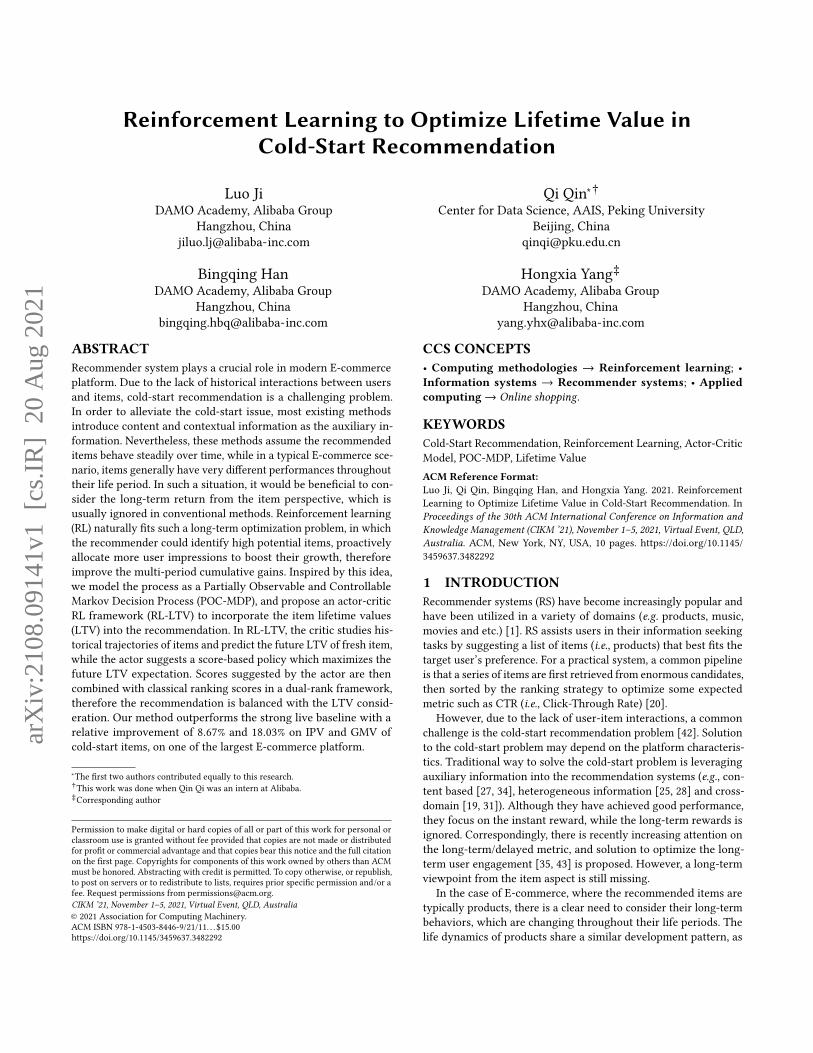
Figure 1: Illustration of the RL-LTV algorithm framework.An RL is employed to solve a item-level MDP and provides apolicy optimizing item long-term rewards (LTV). The policyscore is combined with CTR ranking score with their com-bination weight adjusted by the critic expectation. The ulti-mate ranking score is applied in online ranking.

stated in product life theory [5, 18]. [15] further proposes four dis-tinct stages including introduction, growth, maturity and decline,and uses a mathematical tool to model the product life stages andpredict the transit probability between different stages. In this paper,we also consider the product life dynamics, in a continuous, numer-ical manner. Within the scope of cold-start recommendation, itemson the earlier stages (i.e., introduction and growth) are paid moreattention in this work. For a recently introduced item, recommenda-tion algorithms focus on the instant metric may have the exposurebias. Typically, such fresh items are probably not preferred by theinstant metric due to the lack of historical behavior, therefore theyare subject to low ranking preference. As a result, there might besevere Matthew Effect in the existence of conventional algorithms,in which the mature items keep receiving more impressions andthe fresh items are hard to grow up. However, for some fresh items,they could be more and more popular with some investment of userimpressions, and yield more returns in the future. From this aspect,a smart cold-start recommender should be able to identify high po-tential items in advance, and assign them higher ranking priority;while a low potential product could be penalized in contrary. Amulti-period maximization task is then needed.

Reinforcement Learning (RL) provides a natural, unified frame-work to maximize the instant and long-term rewards jointly andsimultaneously. Nevertheless, considering the complexity of actualonline environment, building an interactive recommender agent be-tween user and item, as well as considering the long-term rewardsis a challenging task. The trial-and-error behavior of RL might harmthe system performance, or affect the user satisfaction. The calcula-tion complexity could also be prohibitively expensive. From theseconsiderations, and considering the fact that the time-evolutionof products are naturally in a much slower time scale than onlinerecommendation (days VS milliseconds), in this study we instead

define an off-policy learning method on the item level and on thedaily basis, which makes the solution practical.

In this paper, we proposes a novel methodology, named rein-forcement learning with lifetime value (RL-LTV), to consider thelong-term rewards of recommended items inside the cold-start rec-ommendation problem. Such long-term rewards are called by itemlifetime values (LTV) in this paper. An off-policy, actor-critic RLwith a recurrent component is employed to learn the item-leveldynamics and make proactive long-term objected decisions. Infor-mation of aforementioned product life stages are encoding by therecurrent hidden memory states, which are studied by a LSTM [16]component, shared by actor and critic. To transfer the informationfrom historical items to cold-start items, we introduce item inherentfeatures, trending bias term, and memory states as extra inputs intoboth the actor and critic. One of the most important action outputby the actor, the item-infinity score of LTV, is then incorporatedwith the conventional ranking score to form a dual-rank frame-work. Their combination weight is determined by action-valuesuggested by the critic. Figure 1 illustrates the entire framework ofour proposed algorithm.

The major contributions of this paper are as follows:

• We define a concept of Partially Observable and ControllableMarkov decision process (POC-MDP) to formulate the productlife dynamics. Unobservable states depict the intrinsic lifestages, while uncontrollable states can affect product growthspeed but are independent of actions.• We incorporate the item LTVs into the online ranking by RL-LTV. By prioritizing high potential cold-start items duringthe ranking, the exposure bias of cold-start items could beovercome. To the best of our knowledge, this is the firsttime that such a technique is applied to solve the cold-startrecommendation problem.• Knowledge of mature items could be generalized and trans-ferred to cold-start items, even for those first-introduceditems. To achieve this, we build the MDP on the item-level,with continual observation and action spaces, as well asparameter-shared policy and critic networks.• We design a learning framework called IE-RDPG to solve alarge-scale RL problem in an itemwise, episodic way. Thealgorithm is deployed into production and improvements of8.67% and 18.03% on IPV and GMV for cold-start items areobserved.

The rest of the paper is organized as follows. The connectionwith previous works is first discussed in Section 2. Preliminariesare then introduced in Section 3. The POC-MDP formulation andits learning algorithm are stated in Section 4. Experiment resultsare summarized in Section 5. Finally Section 6 concludes this paper.

2 RELATEDWORKIn this section, we will briefly review representative works of cold-start recommendation and reinforcement learning.

Cold-start Recommendation: Although collaborative filter-ing and deep learning based model has achieved considerable suc-cess in recommendation systems[17, 21], it is often difficult to dealwith new users or items with few user-item interactions, which is

Reinforcement Learning to Optimize Lifetime Value in Cold-Start Recommendation CIKM ’21, November 1–5, 2021, Virtual Event, QLD, Australia

called cold-start recommendation. The traditional solution of cold-start recommendation is to introduce auxiliary information intothe recommendation system, such as content-based, heterogeneousinformation and cross domain. Specifically, the content-based meth-ods rely on data augmentation by merging the user or item sideinformation [27, 34, 36, 42]. For example, [27] presents an approachnamed visual-CLiMF to learn representative latent factors for cold-start videos, where emotional aspects of items are incorporatedinto the latent factor representations of video contents. [34] pro-poses a hybrid model in which item features are learned from thedescriptions of items via a stacked diagnosing auto-encoder andfurther combined into a collaborative filtering model to address theitem cold-start problem. In addition to these content-based featuresand user-item interactions, richer heterogeneous data is utilizedin the form of heterogeneous information network [10, 25, 29] ,which can capture the interactions between items and other objects.For heterogeneous information based methods, one of the maintasks is to explore the heterogeneous semantics in recommendationsettings by using high-order graph structure, such as Metapathor Metagraph. Finally, cross-domain methods based on transferlearning, which applies the characteristics of the source domain tothe target domain [19, 31]. The premise of this type method is thatthe source domain is available and users or items can be aligned inthe two domains. For example, [19] presents an innovative modelof cross-domain recommendation according to the partial leastsquares regression (PLSR) analysis, which can be utilized for betterprediction of cold-start user ratings. [31] propose a cross-domainlatent feature mappingmodel, where the neighborhood-based cross-domain latent feature mapping method is applied to learn a featuremapping function for each cold-start user.

Although these methods have achieved good performance, mostof them only alleviate the cold-start problem from the single-periodviewpoint while ignore the long-term rewards. Recently, there issome study which tries to study the long-term effect from the user-side [43], but not the item side. In this paper, we try to solve a itemcold-start problem by not only using items content information,but also determine the ranking preference of items according totheir long-term returns.

Reinforcement Learning:Our approach connects to thewidelyapplication of reinforcement learning on recommendation prob-lems. These applications include different strategies: value-based[6, 30, 40], policy-based [7, 12, 14, 26], and model-based [3] methods.When the environment is identified as a partial observable MDP(POMDP), the recurrent neural network is a natural solution todeal with the hidden states [4, 11, 38, 43]. Reinforcement Learningalso helps to generate an end-to-end listwise solution [39] or evenjointly determines the page display arrangement [37].

There are also RL-based studies for cold-start recommenda-tion. [32] proposes an offline meta level model-based method. [9]combines policy-gradient methods and maximum-likelihood ap-proaches and then apply this cold-start reinforcement learningmethod in training sequence generation models for structured out-put prediction problems. [43] uses reinforcement learning to solvethe multi-period reward on user engagement. [15] proposes a RL-based framework for impression allocation, based on consideration

view view

click click

purchase

Pricing

SearchRecommendation

Interested

Crowd

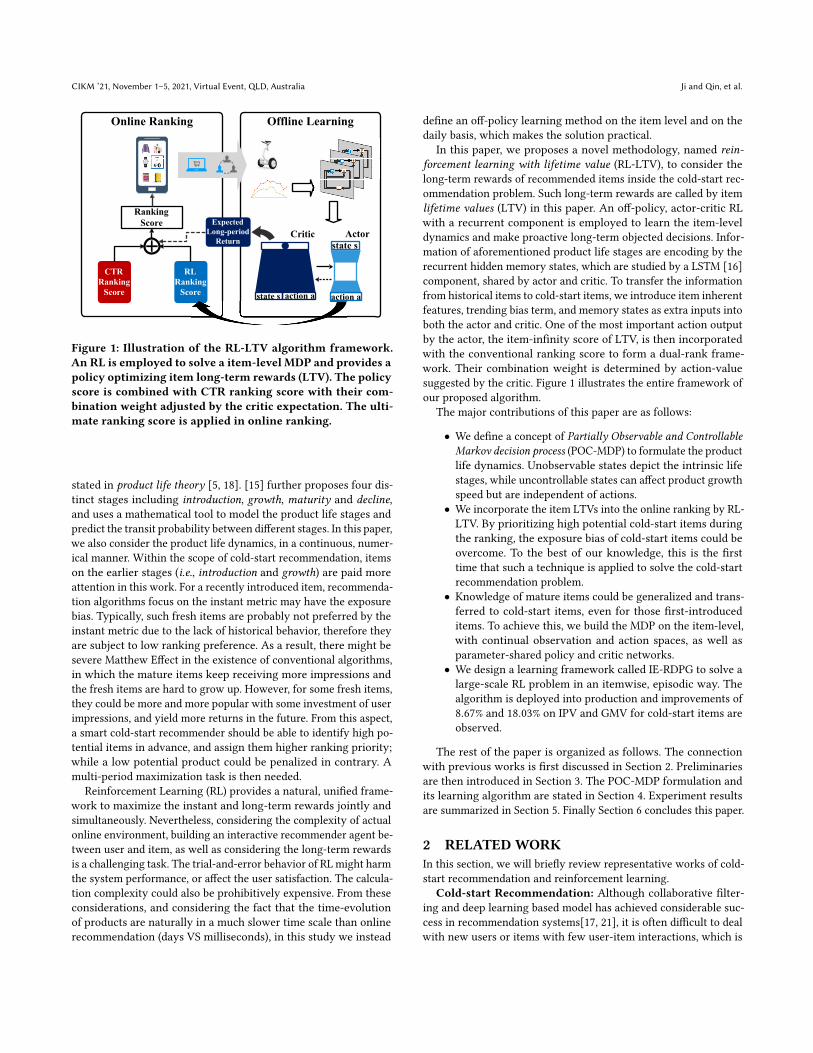
Figure 2: Item metabolism in e-commerce. Recommenda-tion and Search feed the page views of item and determinethe click-through rates. Pricing strategy further determineshow many sales are converted. All of these behaviors re-sult in more people interested with the item and choose tosearch it in the future. The item then obtains more priorityin search and recommendation algorithms because of morehistorical information.

of item life period stages. In their work, the item stages are explic-itly identified and predicted by a mathematical model while RL isused inside the impression allocation problem.

In contrast to [15], in this paper the item stage informationis implicitly studied by reinforcement learning in an end-to-endmanner. In particular, we use recurrent neural network to encodethe hidden state as a continual and dense representation of lifestages, based on item histories. Our framework jointly studies thisrecurrent hidden state, the action value as a prediction of itemlong-term reward, as well as the ranking policy.

3 PRELIMINARIESIn this section, we first introduce the background of product me-tabolism and the idea of item lifetime value on E-commerce, whichbasically motivates this work. Based on the understanding of thisscenario, we define a special type of Markov Decision Process tomodel the metabolism of an item. The basic DDPG algorithm isfinally shown as the underlying learning approach.

3.1 Item Metabolism and Lifetime ValueA typical pattern of product metabolism on the e-commerce plat-form is shown in Figure 2. Assuming a balancing electric scooteris just introduced into the platform, it usually receives few userinterest and the statistics are in low-level. Although the item canbe left to grow up by itself, several channels could be utilized tochange its situation. First, the item’s user exposure (or more specif-ically, the page views (PV)) is significantly affected by both searchand recommendation algorithms. Second, reasonability of searchand recommendation directly affects the click-through rate (CTR),i.e., how many item page views (IPV) could be clicked from PV.


Furthermore, as the third channel, the pricing strategy from thepricing system (PS) has substantial impact that how many numberof sales (SLS) are converted from IPV. During this process, PV, IPVand SLS are accumulated, the item’s reputation is built, and theinterested group of users continues to expand. As more users ap-peal to the item, their behaviors help the specific item claim moreimportance in search and recommendation algorithms, therefore apositive feedback closed-loop mechanism could be created. As itemelapses, the fresh item may have growing life dynamics trajectoriesof key indicators, including PV, IPV and SLS.

However, not all items can achieve such a positive closed-loopmechanism. The growth rate of an item depend on its inherentcharacteristics (what the item is), brand, market, external trendsor noise, and the algorithms. Actually, most items finally fall intothe group called "long-tail products", with few user views, clicks orpurchases. Therefore, it would help if one could identify if the itemcould return significant future PVs, IPVs and GMVs 1, such that thestar products and the long-tail products can be classified even attheir early life stage. In this paper, we call such long-term rewardsas the item’s Lifetime Value (LTV). By allocating more resourcesfor those high potential products, the platform would be repaidwith more LTV in the future, and makes the entire ecosystem growand prosper. As shown in Figure 2, search, recommendation andpricing are possible important tools to allocate the resource andadjust the item dynamics.

3.2 MDP and its ExtensionsMarkov Decision Process (MDP) is typically employed to model thesequential decision making problem. Nominal MDP usually consistsof the 4-tuple (S,A,R,P), where S,A,R,P are the state space,action space, set of rewards, and transition probability functions,respectively. At time step 𝑡 , the state 𝑠𝑡 ∈ S represents the currentsystem stage, which is affected by an action 𝑎𝑡 ∈ A from the agent,generating a reward 𝑟𝑡 by the reward function S × A → R, aswell as the next state 𝑠𝑡+1 ∈ P(𝑠𝑡 , 𝑎𝑡 ). For such nominal MDP, itassumes that all elements of 𝑠 can both be observed by agent, andbe changed by the agent’s action.

However, it is rare that this assumption holds in the real en-vironment. For example, the Pong game in Atari have both thecurrent image and the ball velocity as state, while only the formeris provided to the agent. Partially Observable Markov Decision Pro-cess (PO-MDP) captures the partial observability part of systemcomplexity. It is instead described as a 5-tuple (S,A,P,R,O), inwhich O denotes the set of observable states, i.e., O is subset of S.

Another form of system complexity is relatively less studied,the MDP with uncontrollable states [2, 22]. In such situations, someelements of 𝑠𝑡 can never be affected by agent actions, but they candetermines 𝑠𝑡+1 therefore affect future rewards too. We here payespecial attention to such form of uncontrollablity, which will bediscussed with more details in the next section.

In our topic, it is believed that both unobservable and uncontrol-lable states exist, both of which are discussed with more details inSection 4. We deal with the above concerns and define a PartiallyObservable and Controllable Markov Decision Process (POC-MDP),

1The gross merchandise value from the item, which equals to 𝑆𝐿𝑆 times the averagedpaid price.

which literally means there are some unobservable states and someuncontrollable states in MDP at the same time. Although the term"state" can denote all states no matter they are observable or control-lable, for clarity, we use the notation 𝑠 to present only the nominal(both observable and controllable) states. The unobservable states(but controllable) are denoted byℎ ∈ H , and the uncontrollable (butobservable) states are denoted by 𝑥 ∈ X. As a result, our POC-MDPnow has the 6-tuple (S,A,P,R,O,H). Note now the observationis the concatenation of nominal states and uncontrollable states2,i.e., 𝑜 := [𝑠, 𝑥].

3.3 The DDPG methodIn this section we give a brief introduction to an model-free, off-policy, actor-crtic RL algorithm, the Deep Deterministic Policy Gra-dient (DDPG) method [23], which is closely related to our proposedapproach.

In DDPG, the actor network 𝜋 is approximated by the net pa-rameter \ and generates the policy, and the critic network 𝑄 isapproximated by the net parameter 𝑤 and generates the action-value function. Gradients of the deterministic policy is

▽\ 𝐽 = E𝑠∽𝑑𝜋 [▽\𝜋\ (𝑠)▽𝑎𝑄𝑤 (𝑠, 𝑎) |𝑎=𝜋 (𝑠) ]

where 𝑑𝜋 (𝑠) is a discounted distribution of state 𝑠 under the policyof 𝜋 . Then \ can be updated as

\ ← \ + [E𝑠∽𝑑𝜋 [▽\𝜋\ (𝑠)▽𝑎𝑄𝑤 (𝑠, 𝑎) |𝑎=𝜋 (𝑠) ]

with [ as the learning rate. For the critic, the action-value functioncan be obtained iteratively as

𝑄𝑤 (𝑠𝑡 , 𝑎𝑡 ) = E[𝑟𝑡 + 𝛾E𝑎∽𝜋\ [𝑄𝑤 (𝑠𝑡+1, 𝑎𝑡+1)]]

𝑤 is updated by minimizing the following objective function

min𝑤𝐿 = E𝑠∽𝑑𝜋 [(𝑅(𝑠𝑡 , 𝑎𝑡 )+𝛾𝑄𝑤

′ (𝑠𝑡+1, 𝜋\ ′ (𝑠𝑡+1))−𝑄𝑤 (𝑠𝑡 , 𝜋\ (𝑠𝑡 )))2]

where 𝜋\ ′ and 𝑄𝑤′ are the target networks of actor and critic. The

target network parameters can be softly updated by

\`′←𝜏\`

′+ (1 − 𝜏)\`

𝑤′← 𝜏𝑤

′+ (1 − 𝜏)𝑤

4 METHODThis section illustrates the key concepts of our approach, includinghow we implement our RL-LTV, and how its action is applied inthe online system. First definitions of terms in POC-MDP are listed,then architectures of the actor and critic networks are introduced,after which the learning algorithm follows. The actor outputs apreference score, which is linearly combined with the ranking scorefrom a conventional CTR model in a dual rank framework. Thenew ranking score is then applied to sort items within the responseto each request. Table 1 summarizes important symbols which arefrequently used in the current and related sections.

2In this paper, we use the square bracket to represent the concatenation of multiplevariables, for simplicity.


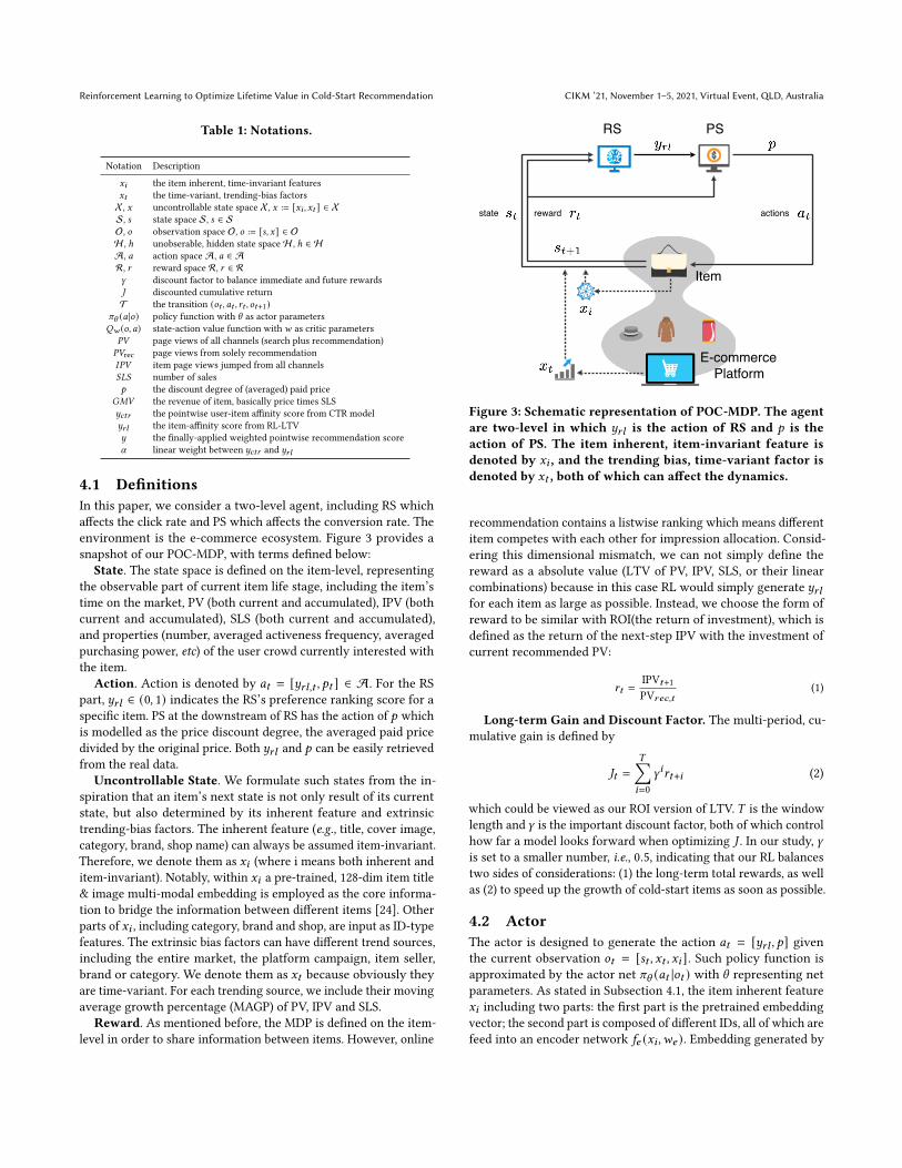
Table 1: Notations.

Notation Description

𝑥𝑖 the item inherent, time-invariant features𝑥𝑡 the time-variant, trending-bias factorsX, 𝑥 uncontrollable state space X, 𝑥 := [𝑥𝑖 , 𝑥𝑡 ] ∈ XS, 𝑠 state space S, 𝑠 ∈ SO, 𝑜 observation space O, 𝑜 := [𝑠, 𝑥] ∈ OH , ℎ unobserable, hidden state spaceH , ℎ ∈ HA, 𝑎 action space A, 𝑎 ∈ AR, 𝑟 reward space R, 𝑟 ∈ R𝛾 discount factor to balance immediate and future rewards𝐽 discounted cumulative returnT the transition (𝑜𝑡 , 𝑎𝑡 , 𝑟𝑡 , 𝑜𝑡+1)

𝜋\ (𝑎 |𝑜) policy function with \ as actor parameters𝑄𝑤 (𝑜, 𝑎) state-action value function with𝑤 as critic parameters𝑃𝑉 page views of all channels (search plus recommendation)𝑃𝑉rec page views from solely recommendation𝐼𝑃𝑉 item page views jumped from all channels𝑆𝐿𝑆 number of sales𝑝 the discount degree of (averaged) paid price

𝐺𝑀𝑉 the revenue of item, basically price times SLS𝑦𝑐𝑡𝑟 the pointwise user-item affinity score from CTR model𝑦𝑟𝑙 the item-affinity score from RL-LTV𝑦 the finally-applied weighted pointwise recommendation score𝛼 linear weight between 𝑦𝑐𝑡𝑟 and 𝑦𝑟𝑙

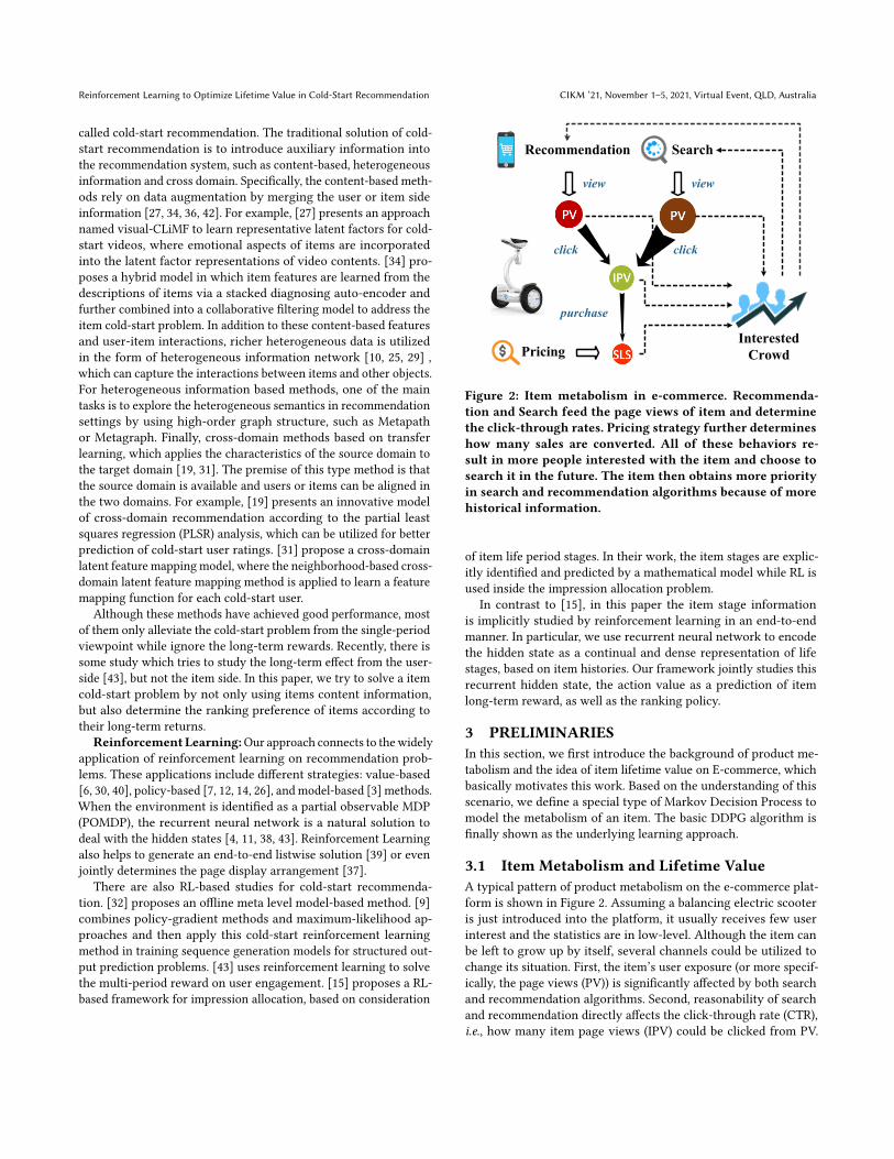
4.1 DefinitionsIn this paper, we consider a two-level agent, including RS whichaffects the click rate and PS which affects the conversion rate. Theenvironment is the e-commerce ecosystem. Figure 3 provides asnapshot of our POC-MDP, with terms defined below:

State. The state space is defined on the item-level, representingthe observable part of current item life stage, including the item’stime on the market, PV (both current and accumulated), IPV (bothcurrent and accumulated), SLS (both current and accumulated),and properties (number, averaged activeness frequency, averagedpurchasing power, etc) of the user crowd currently interested withthe item.

Action. Action is denoted by 𝑎𝑡 = [𝑦𝑟𝑙,𝑡 , 𝑝𝑡 ] ∈ A. For the RSpart, 𝑦𝑟𝑙 ∈ (0, 1) indicates the RS’s preference ranking score for aspecific item. PS at the downstream of RS has the action of 𝑝 whichis modelled as the price discount degree, the averaged paid pricedivided by the original price. Both 𝑦𝑟𝑙 and 𝑝 can be easily retrievedfrom the real data.

Uncontrollable State. We formulate such states from the in-spiration that an item’s next state is not only result of its currentstate, but also determined by its inherent feature and extrinsictrending-bias factors. The inherent feature (e.g., title, cover image,category, brand, shop name) can always be assumed item-invariant.Therefore, we denote them as 𝑥𝑖 (where i means both inherent anditem-invariant). Notably, within 𝑥𝑖 a pre-trained, 128-dim item title& image multi-modal embedding is employed as the core informa-tion to bridge the information between different items [24]. Otherparts of 𝑥𝑖 , including category, brand and shop, are input as ID-typefeatures. The extrinsic bias factors can have different trend sources,including the entire market, the platform campaign, item seller,brand or category. We denote them as 𝑥𝑡 because obviously theyare time-variant. For each trending source, we include their movingaverage growth percentage (MAGP) of PV, IPV and SLS.

Reward. As mentioned before, the MDP is defined on the item-level in order to share information between items. However, online

actions

RS PS

E-commerce Platform

Item

state reward

Figure 3: Schematic representation of POC-MDP. The agentare two-level in which 𝑦𝑟𝑙 is the action of RS and 𝑝 is theaction of PS. The item inherent, item-invariant feature isdenoted by 𝑥𝑖 , and the trending bias, time-variant factor isdenoted by 𝑥𝑡 , both of which can affect the dynamics.

recommendation contains a listwise ranking which means differentitem competes with each other for impression allocation. Consid-ering this dimensional mismatch, we can not simply define thereward as a absolute value (LTV of PV, IPV, SLS, or their linearcombinations) because in this case RL would simply generate 𝑦𝑟𝑙for each item as large as possible. Instead, we choose the form ofreward to be similar with ROI(the return of investment), which isdefined as the return of the next-step IPV with the investment ofcurrent recommended PV:

𝑟𝑡 =IPV𝑡+1PV𝑟𝑒𝑐,𝑡

(1)

Long-term Gain and Discount Factor. The multi-period, cu-mulative gain is defined by

𝐽𝑡 =

𝑇∑︁𝑖=0

𝛾𝑖𝑟𝑡+𝑖 (2)

which could be viewed as our ROI version of LTV. 𝑇 is the windowlength and 𝛾 is the important discount factor, both of which controlhow far a model looks forward when optimizing 𝐽 . In our study, 𝛾is set to a smaller number, i.e., 0.5, indicating that our RL balancestwo sides of considerations: (1) the long-term total rewards, as wellas (2) to speed up the growth of cold-start items as soon as possible.

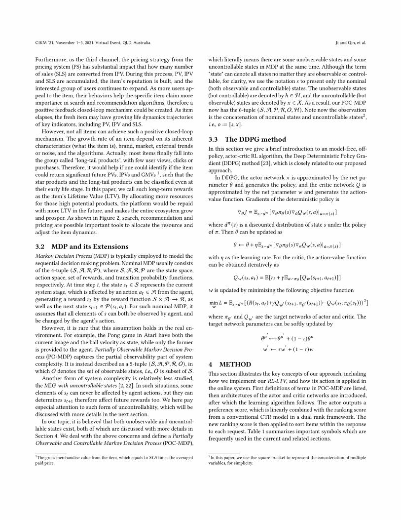
4.2 ActorThe actor is designed to generate the action 𝑎𝑡 = [𝑦𝑟𝑙 , 𝑝] giventhe current observation 𝑜𝑡 = [𝑠𝑡 , 𝑥𝑡 , 𝑥𝑖 ]. Such policy function isapproximated by the actor net 𝜋\ (𝑎𝑡 |𝑜𝑡 ) with \ representing netparameters. As stated in Subsection 4.1, the item inherent feature𝑥𝑖 including two parts: the first part is the pretrained embeddingvector; the second part is composed of different IDs, all of which arefeed into an encoder network 𝑓𝑒 (𝑥𝑖 ,𝑤𝑒 ). Embedding generated by


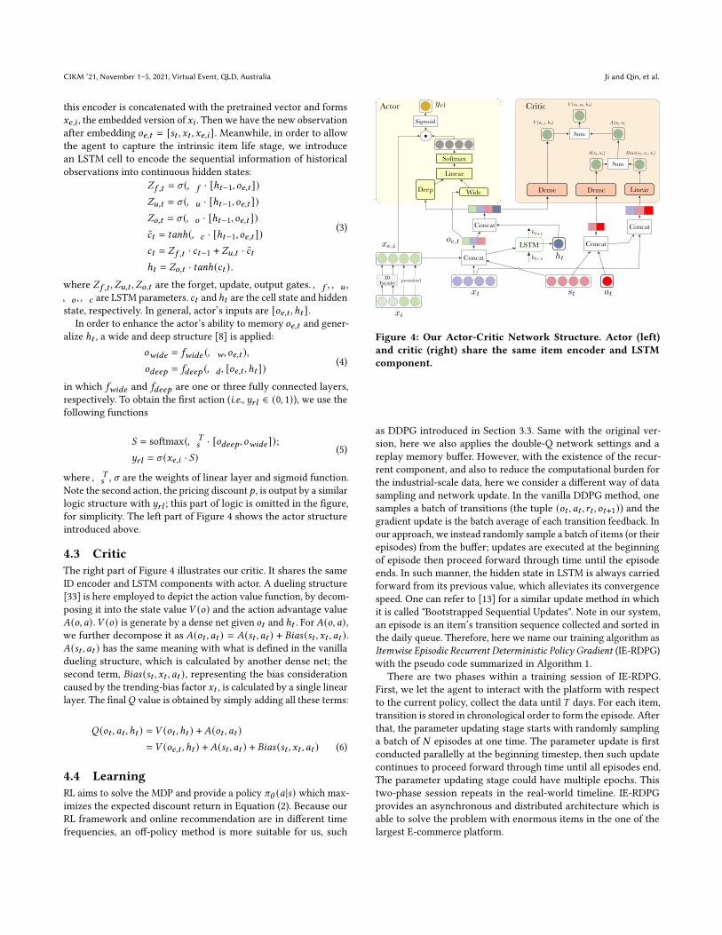
this encoder is concatenated with the pretrained vector and forms𝑥𝑒,𝑖 , the embedded version of 𝑥𝑖 . Then we have the new observationafter embedding 𝑜𝑒,𝑡 = [𝑠𝑡 , 𝑥𝑡 , 𝑥𝑒,𝑖 ]. Meanwhile, in order to allowthe agent to capture the intrinsic item life stage, we introducean LSTM cell to encode the sequential information of historicalobservations into continuous hidden states:

𝑍 𝑓 ,𝑡 = 𝜎 (𝑊𝑓 · [ℎ𝑡−1, 𝑜𝑒,𝑡 ])𝑍𝑢,𝑡 = 𝜎 (𝑊𝑢 · [ℎ𝑡−1, 𝑜𝑒,𝑡 ])𝑍𝑜,𝑡 = 𝜎 (𝑊𝑜 · [ℎ𝑡−1, 𝑜𝑒,𝑡 ])𝑐𝑡 = 𝑡𝑎𝑛ℎ(𝑊𝑐 · [ℎ𝑡−1, 𝑜𝑒,𝑡 ])𝑐𝑡 = 𝑍 𝑓 ,𝑡 · 𝑐𝑡−1 + 𝑍𝑢,𝑡 · 𝑐𝑡ℎ𝑡 = 𝑍𝑜,𝑡 · 𝑡𝑎𝑛ℎ(𝑐𝑡 ).

(3)

where 𝑍 𝑓 ,𝑡 , 𝑍𝑢,𝑡 , 𝑍𝑜,𝑡 are the forget, update, output gates.𝑊𝑓 ,𝑊𝑢 ,𝑊𝑜 ,𝑊𝑐 are LSTM parameters. 𝑐𝑡 and ℎ𝑡 are the cell state and hiddenstate, respectively. In general, actor’s inputs are [𝑜𝑒,𝑡 , ℎ𝑡 ].

In order to enhance the actor’s ability to memory 𝑜𝑒,𝑡 and gener-alize ℎ𝑡 , a wide and deep structure [8] is applied:

𝑜𝑤𝑖𝑑𝑒 = 𝑓𝑤𝑖𝑑𝑒 (𝑊𝑤 , 𝑜𝑒,𝑡 ),𝑜𝑑𝑒𝑒𝑝 = 𝑓𝑑𝑒𝑒𝑝 (𝑊𝑑 , [𝑜𝑒,𝑡 , ℎ𝑡 ])

(4)

in which 𝑓𝑤𝑖𝑑𝑒 and 𝑓𝑑𝑒𝑒𝑝 are one or three fully connected layers,respectively. To obtain the first action (i.e., 𝑦𝑟𝑙 ∈ (0, 1)), we use thefollowing functions

𝑆 = softmax(𝑊𝑇𝑠 · [𝑜𝑑𝑒𝑒𝑝 , 𝑜𝑤𝑖𝑑𝑒 ]);

𝑦𝑟𝑙 = 𝜎 (𝑥𝑒,𝑖 · 𝑆)(5)

where𝑊𝑇𝑠 , 𝜎 are the weights of linear layer and sigmoid function.

Note the second action, the pricing discount 𝑝 , is output by a similarlogic structure with 𝑦𝑟𝑙 ; this part of logic is omitted in the figure,for simplicity. The left part of Figure 4 shows the actor structureintroduced above.

4.3 CriticThe right part of Figure 4 illustrates our critic. It shares the sameID encoder and LSTM components with actor. A dueling structure[33] is here employed to depict the action value function, by decom-posing it into the state value 𝑉 (𝑜) and the action advantage value𝐴(𝑜, 𝑎).𝑉 (𝑜) is generate by a dense net given 𝑜𝑡 and ℎ𝑡 . For𝐴(𝑜, 𝑎),we further decompose it as 𝐴(𝑜𝑡 , 𝑎𝑡 ) = 𝐴(𝑠𝑡 , 𝑎𝑡 ) + 𝐵𝑖𝑎𝑠 (𝑠𝑡 , 𝑥𝑡 , 𝑎𝑡 ).𝐴(𝑠𝑡 , 𝑎𝑡 ) has the same meaning with what is defined in the vanilladueling structure, which is calculated by another dense net; thesecond term, 𝐵𝑖𝑎𝑠 (𝑠𝑡 , 𝑥𝑡 , 𝑎𝑡 ), representing the bias considerationcaused by the trending-bias factor 𝑥𝑡 , is calculated by a single linearlayer. The final𝑄 value is obtained by simply adding all these terms:

𝑄 (𝑜𝑡 , 𝑎𝑡 , ℎ𝑡 ) = 𝑉 (𝑜𝑡 , ℎ𝑡 ) +𝐴(𝑜𝑡 , 𝑎𝑡 )= 𝑉 (𝑜𝑒,𝑡 , ℎ𝑡 ) +𝐴(𝑠𝑡 , 𝑎𝑡 ) + 𝐵𝑖𝑎𝑠 (𝑠𝑡 , 𝑥𝑡 , 𝑎𝑡 ) (6)

4.4 LearningRL aims to solve the MDP and provide a policy 𝜋\ (𝑎 |𝑠) which max-imizes the expected discount return in Equation (2). Because ourRL framework and online recommendation are in different timefrequencies, an off-policy method is more suitable for us, such

Actor Critic

st atxt

xi

LSTM

ht−1

ht+1

ht

Deep Wide Linear

yrl

Dense

IDEncoder

Softmax

Linear

Concat

Concat

Concat

Dense

Sum

SUM

Concat

Concat

Sum

Sigmoid

xe,ioe,t

Bias(st, xt, xt)A(st, at)

A(ot, at)V (oe,t, ht)

V (ot, at, ht)

pretrained

Figure 4: Our Actor-Critic Network Structure. Actor (left)and critic (right) share the same item encoder and LSTMcomponent.

as DDPG introduced in Section 3.3. Same with the original ver-sion, here we also applies the double-Q network settings and areplay memory buffer. However, with the existence of the recur-rent component, and also to reduce the computational burden forthe industrial-scale data, here we consider a different way of datasampling and network update. In the vanilla DDPG method, onesamples a batch of transitions (the tuple (𝑜𝑡 , 𝑎𝑡 , 𝑟𝑡 , 𝑜𝑡+1)) and thegradient update is the batch average of each transition feedback. Inour approach, we instead randomly sample a batch of items (or theirepisodes) from the buffer; updates are executed at the beginningof episode then proceed forward through time until the episodeends. In such manner, the hidden state in LSTM is always carriedforward from its previous value, which alleviates its convergencespeed. One can refer to [13] for a similar update method in whichit is called "Bootstrapped Sequential Updates". Note in our system,an episode is an item’s transition sequence collected and sorted inthe daily queue. Therefore, here we name our training algorithm asItemwise Episodic Recurrent Deterministic Policy Gradient (IE-RDPG)with the pseudo code summarized in Algorithm 1.

There are two phases within a training session of IE-RDPG.First, we let the agent to interact with the platform with respectto the current policy, collect the data until 𝑇 days. For each item,transition is stored in chronological order to form the episode. Afterthat, the parameter updating stage starts with randomly samplinga batch of 𝑁 episodes at one time. The parameter update is firstconducted parallelly at the beginning timestep, then such updatecontinues to proceed forward through time until all episodes end.The parameter updating stage could have multiple epochs. Thistwo-phase session repeats in the real-world timeline. IE-RDPGprovides an asynchronous and distributed architecture which isable to solve the problem with enormous items in the one of thelargest E-commerce platform.


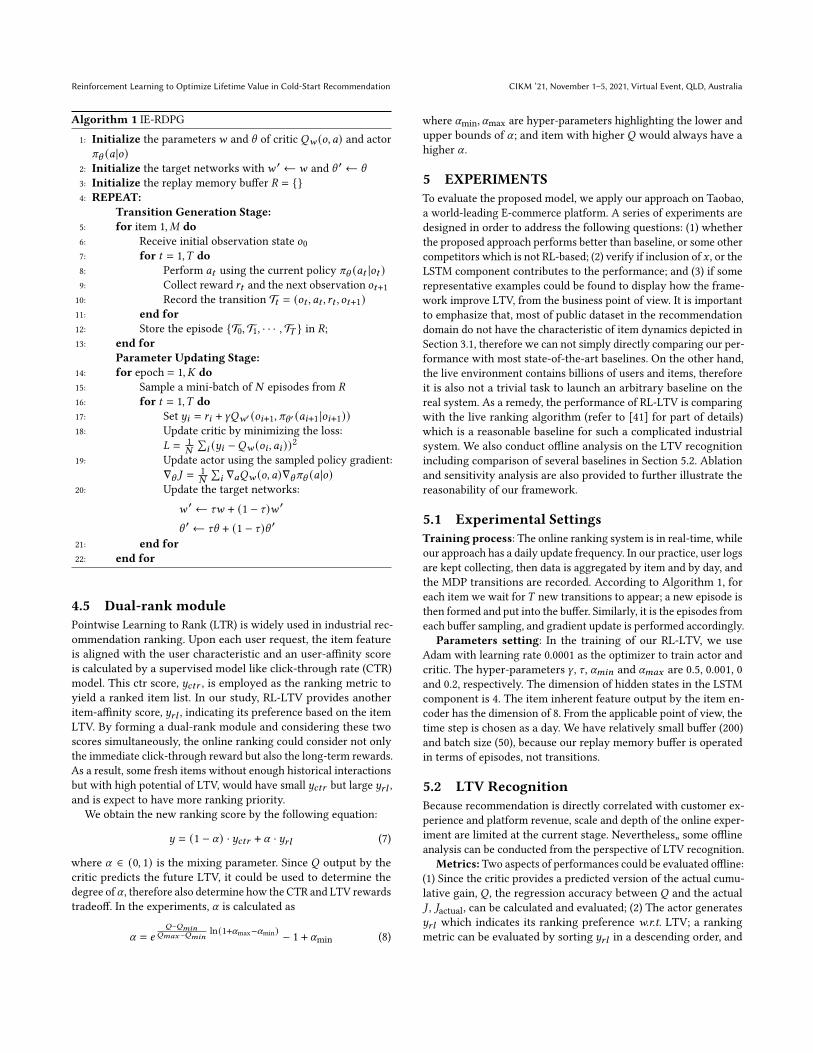
Algorithm 1 IE-RDPG

1: Initialize the parameters𝑤 and \ of critic 𝑄𝑤 (𝑜, 𝑎) and actor𝜋\ (𝑎 |𝑜)

2: Initialize the target networks with𝑤 ′ ← 𝑤 and \ ′ ← \

3: Initialize the replay memory buffer 𝑅 = {}4: REPEAT:

Transition Generation Stage:5: for item 1, 𝑀 do6: Receive initial observation state 𝑜07: for 𝑡 = 1,𝑇 do8: Perform 𝑎𝑡 using the current policy 𝜋\ (𝑎𝑡 |𝑜𝑡 )9: Collect reward 𝑟𝑡 and the next observation 𝑜𝑡+110: Record the transition T𝑡 = (𝑜𝑡 , 𝑎𝑡 , 𝑟𝑡 , 𝑜𝑡+1)11: end for12: Store the episode {T0,T1, · · · ,T𝑇 } in 𝑅;13: end for

Parameter Updating Stage:14: for epoch = 1, 𝐾 do15: Sample a mini-batch of 𝑁 episodes from 𝑅

16: for 𝑡 = 1,𝑇 do17: Set 𝑦𝑖 = 𝑟𝑖 + 𝛾𝑄𝑤′ (𝑜𝑖+1, 𝜋\ ′ (𝑎𝑖+1 |𝑜𝑖+1))18: Update critic by minimizing the loss:

𝐿 = 1𝑁

∑𝑖 (𝑦𝑖 −𝑄𝑤 (𝑜𝑖 , 𝑎𝑖 ))2

19: Update actor using the sampled policy gradient:∇\ 𝐽 = 1

𝑁

∑𝑖 ∇𝑎𝑄𝑤 (𝑜, 𝑎)∇\𝜋\ (𝑎 |𝑜)

20: Update the target networks:

𝑤 ′ ← 𝜏𝑤 + (1 − 𝜏)𝑤 ′

\ ′ ← 𝜏\ + (1 − 𝜏)\ ′21: end for22: end for

4.5 Dual-rank modulePointwise Learning to Rank (LTR) is widely used in industrial rec-ommendation ranking. Upon each user request, the item featureis aligned with the user characteristic and an user-affinity scoreis calculated by a supervised model like click-through rate (CTR)model. This ctr score, 𝑦𝑐𝑡𝑟 , is employed as the ranking metric toyield a ranked item list. In our study, RL-LTV provides anotheritem-affinity score, 𝑦𝑟𝑙 , indicating its preference based on the itemLTV. By forming a dual-rank module and considering these twoscores simultaneously, the online ranking could consider not onlythe immediate click-through reward but also the long-term rewards.As a result, some fresh items without enough historical interactionsbut with high potential of LTV, would have small 𝑦𝑐𝑡𝑟 but large 𝑦𝑟𝑙 ,and is expect to have more ranking priority.

We obtain the new ranking score by the following equation:

𝑦 = (1 − 𝛼) · 𝑦𝑐𝑡𝑟 + 𝛼 · 𝑦𝑟𝑙 (7)

where 𝛼 ∈ (0, 1) is the mixing parameter. Since 𝑄 output by thecritic predicts the future LTV, it could be used to determine thedegree of𝛼 , therefore also determine how the CTR and LTV rewardstradeoff. In the experiments, 𝛼 is calculated as

𝛼 = 𝑒𝑄−𝑄𝑚𝑖𝑛

𝑄𝑚𝑎𝑥 −𝑄𝑚𝑖𝑛ln(1+𝛼max−𝛼min) − 1 + 𝛼min (8)

where 𝛼min, 𝛼max are hyper-parameters highlighting the lower andupper bounds of 𝛼 ; and item with higher 𝑄 would always have ahigher 𝛼 .

5 EXPERIMENTSTo evaluate the proposed model, we apply our approach on Taobao,a world-leading E-commerce platform. A series of experiments aredesigned in order to address the following questions: (1) whetherthe proposed approach performs better than baseline, or some othercompetitors which is not RL-based; (2) verify if inclusion of 𝑥 , or theLSTM component contributes to the performance; and (3) if somerepresentative examples could be found to display how the frame-work improve LTV, from the business point of view. It is importantto emphasize that, most of public dataset in the recommendationdomain do not have the characteristic of item dynamics depicted inSection 3.1, therefore we can not simply directly comparing our per-formance with most state-of-the-art baselines. On the other hand,the live environment contains billions of users and items, thereforeit is also not a trivial task to launch an arbitrary baseline on thereal system. As a remedy, the performance of RL-LTV is comparingwith the live ranking algorithm (refer to [41] for part of details)which is a reasonable baseline for such a complicated industrialsystem. We also conduct offline analysis on the LTV recognitionincluding comparison of several baselines in Section 5.2. Ablationand sensitivity analysis are also provided to further illustrate thereasonability of our framework.

5.1 Experimental SettingsTraining process: The online ranking system is in real-time, whileour approach has a daily update frequency. In our practice, user logsare kept collecting, then data is aggregated by item and by day, andthe MDP transitions are recorded. According to Algorithm 1, foreach item we wait for𝑇 new transitions to appear; a new episode isthen formed and put into the buffer. Similarly, it is the episodes fromeach buffer sampling, and gradient update is performed accordingly.

Parameters setting: In the training of our RL-LTV, we useAdam with learning rate 0.0001 as the optimizer to train actor andcritic. The hyper-parameters 𝛾 , 𝜏 , 𝛼𝑚𝑖𝑛 and 𝛼𝑚𝑎𝑥 are 0.5, 0.001, 0and 0.2, respectively. The dimension of hidden states in the LSTMcomponent is 4. The item inherent feature output by the item en-coder has the dimension of 8. From the applicable point of view, thetime step is chosen as a day. We have relatively small buffer (200)and batch size (50), because our replay memory buffer is operatedin terms of episodes, not transitions.

5.2 LTV RecognitionBecause recommendation is directly correlated with customer ex-perience and platform revenue, scale and depth of the online exper-iment are limited at the current stage. Nevertheless„ some offlineanalysis can be conducted from the perspective of LTV recognition.

Metrics: Two aspects of performances could be evaluated offline:(1) Since the critic provides a predicted version of the actual cumu-lative gain, 𝑄 , the regression accuracy between 𝑄 and the actual𝐽 , 𝐽actual, can be calculated and evaluated; (2) The actor generates𝑦𝑟𝑙 which indicates its ranking preference w.r.t. LTV; a rankingmetric can be evaluated by sorting 𝑦𝑟𝑙 in a descending order, and


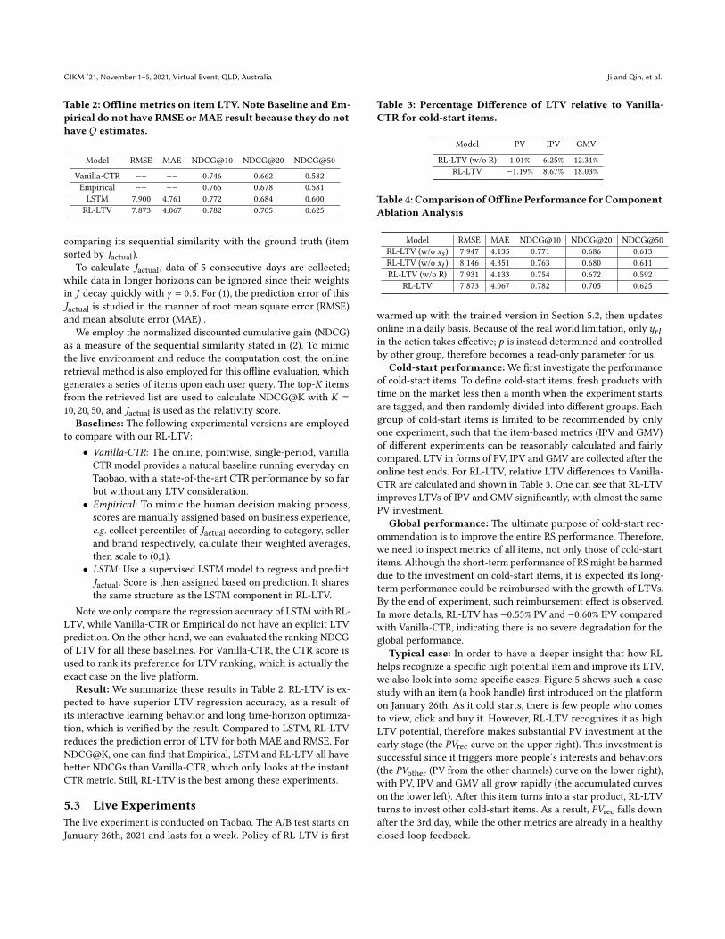
Table 2: Offline metrics on item LTV. Note Baseline and Em-pirical do not have RMSE or MAE result because they do nothave 𝑄 estimates.

Model RMSE MAE NDCG@10 NDCG@20 NDCG@50

Vanilla-CTR −− −− 0.746 0.662 0.582Empirical −− −− 0.765 0.678 0.581LSTM 7.900 4.761 0.772 0.684 0.600RL-LTV 7.873 4.067 0.782 0.705 0.625

comparing its sequential similarity with the ground truth (itemsorted by 𝐽actual).

To calculate 𝐽actual, data of 5 consecutive days are collected;while data in longer horizons can be ignored since their weightsin 𝐽 decay quickly with 𝛾 = 0.5. For (1), the prediction error of this𝐽actual is studied in the manner of root mean square error (RMSE)and mean absolute error (MAE) .

We employ the normalized discounted cumulative gain (NDCG)as a measure of the sequential similarity stated in (2). To mimicthe live environment and reduce the computation cost, the onlineretrieval method is also employed for this offline evaluation, whichgenerates a series of items upon each user query. The top-𝐾 itemsfrom the retrieved list are used to calculate NDCG@K with 𝐾 =

10, 20, 50, and 𝐽actual is used as the relativity score.Baselines: The following experimental versions are employed

to compare with our RL-LTV:• Vanilla-CTR: The online, pointwise, single-period, vanillaCTR model provides a natural baseline running everyday onTaobao, with a state-of-the-art CTR performance by so farbut without any LTV consideration.• Empirical: To mimic the human decision making process,scores are manually assigned based on business experience,e.g. collect percentiles of 𝐽actual according to category, sellerand brand respectively, calculate their weighted averages,then scale to (0,1).• LSTM: Use a supervised LSTM model to regress and predict𝐽actual. Score is then assigned based on prediction. It sharesthe same structure as the LSTM component in RL-LTV.

Note we only compare the regression accuracy of LSTM with RL-LTV, while Vanilla-CTR or Empirical do not have an explicit LTVprediction. On the other hand, we can evaluated the ranking NDCGof LTV for all these baselines. For Vanilla-CTR, the CTR score isused to rank its preference for LTV ranking, which is actually theexact case on the live platform.

Result: We summarize these results in Table 2. RL-LTV is ex-pected to have superior LTV regression accuracy, as a result ofits interactive learning behavior and long time-horizon optimiza-tion, which is verified by the result. Compared to LSTM, RL-LTVreduces the prediction error of LTV for both MAE and RMSE. ForNDCG@K, one can find that Empirical, LSTM and RL-LTV all havebetter NDCGs than Vanilla-CTR, which only looks at the instantCTR metric. Still, RL-LTV is the best among these experiments.

5.3 Live ExperimentsThe live experiment is conducted on Taobao. The A/B test starts onJanuary 26th, 2021 and lasts for a week. Policy of RL-LTV is first

Table 3: Percentage Difference of LTV relative to Vanilla-CTR for cold-start items.

Model PV IPV GMV

RL-LTV (w/o R) 1.01% 6.25% 12.31%RL-LTV −1.19% 8.67% 18.03%

Table 4: Comparison ofOffline Performance forComponentAblation Analysis

Model RMSE MAE NDCG@10 NDCG@20 NDCG@50RL-LTV (w/o 𝑥𝑠 ) 7.947 4.135 0.771 0.686 0.613RL-LTV (w/o 𝑥𝑡 ) 8.146 4.351 0.763 0.680 0.611RL-LTV (w/o R) 7.931 4.133 0.754 0.672 0.592

RL-LTV 7.873 4.067 0.782 0.705 0.625

warmed up with the trained version in Section 5.2, then updatesonline in a daily basis. Because of the real world limitation, only 𝑦𝑟𝑙in the action takes effective; 𝑝 is instead determined and controlledby other group, therefore becomes a read-only parameter for us.

Cold-start performance:We first investigate the performanceof cold-start items. To define cold-start items, fresh products withtime on the market less then a month when the experiment startsare tagged, and then randomly divided into different groups. Eachgroup of cold-start items is limited to be recommended by onlyone experiment, such that the item-based metrics (IPV and GMV)of different experiments can be reasonably calculated and fairlycompared. LTV in forms of PV, IPV and GMV are collected after theonline test ends. For RL-LTV, relative LTV differences to Vanilla-CTR are calculated and shown in Table 3. One can see that RL-LTVimproves LTVs of IPV and GMV significantly, with almost the samePV investment.

Global performance: The ultimate purpose of cold-start rec-ommendation is to improve the entire RS performance. Therefore,we need to inspect metrics of all items, not only those of cold-startitems. Although the short-term performance of RS might be harmeddue to the investment on cold-start items, it is expected its long-term performance could be reimbursed with the growth of LTVs.By the end of experiment, such reimbursement effect is observed.In more details, RL-LTV has −0.55% PV and −0.60% IPV comparedwith Vanilla-CTR, indicating there is no severe degradation for theglobal performance.

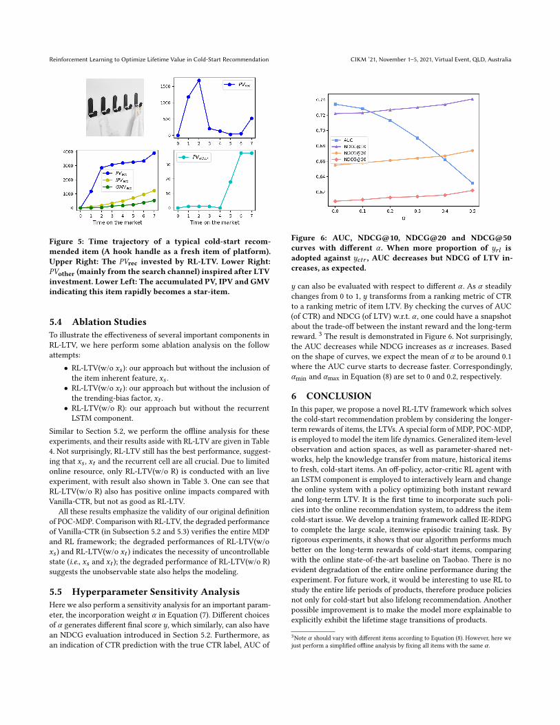
Typical case: In order to have a deeper insight that how RLhelps recognize a specific high potential item and improve its LTV,we also look into some specific cases. Figure 5 shows such a casestudy with an item (a hook handle) first introduced on the platformon January 26th. As it cold starts, there is few people who comesto view, click and buy it. However, RL-LTV recognizes it as highLTV potential, therefore makes substantial PV investment at theearly stage (the 𝑃𝑉rec curve on the upper right). This investment issuccessful since it triggers more people’s interests and behaviors(the 𝑃𝑉other (PV from the other channels) curve on the lower right),with PV, IPV and GMV all grow rapidly (the accumulated curveson the lower left). After this item turns into a star product, RL-LTVturns to invest other cold-start items. As a result, 𝑃𝑉rec falls downafter the 3rd day, while the other metrics are already in a healthyclosed-loop feedback.


Figure 5: Time trajectory of a typical cold-start recom-mended item (A hook handle as a fresh item of platform).Upper Right: The 𝑃𝑉rec invested by RL-LTV. Lower Right:𝑃𝑉other (mainly from the search channel) inspired after LTVinvestment. Lower Left: The accumulated PV, IPV and GMVindicating this item rapidly becomes a star-item.

5.4 Ablation StudiesTo illustrate the effectiveness of several important components inRL-LTV, we here perform some ablation analysis on the followattempts:• RL-LTV(w/o 𝑥𝑠 ): our approach but without the inclusion ofthe item inherent feature, 𝑥𝑠 .• RL-LTV(w/o 𝑥𝑡 ): our approach but without the inclusion ofthe trending-bias factor, 𝑥𝑡 .• RL-LTV(w/o R): our approach but without the recurrentLSTM component.

Similar to Section 5.2, we perform the offline analysis for theseexperiments, and their results aside with RL-LTV are given in Table4. Not surprisingly, RL-LTV still has the best performance, suggest-ing that 𝑥𝑠 , 𝑥𝑡 and the recurrent cell are all crucial. Due to limitedonline resource, only RL-LTV(w/o R) is conducted with an liveexperiment, with result also shown in Table 3. One can see thatRL-LTV(w/o R) also has positive online impacts compared withVanilla-CTR, but not as good as RL-LTV.

All these results emphasize the validity of our original definitionof POC-MDP. Comparison with RL-LTV, the degraded performanceof Vanilla-CTR (in Subsection 5.2 and 5.3) verifies the entire MDPand RL framework; the degraded performances of RL-LTV(w/o𝑥𝑠 ) and RL-LTV(w/o 𝑥𝑡 ) indicates the necessity of uncontrollablestate (i.e., 𝑥𝑠 and 𝑥𝑡 ); the degraded performance of RL-LTV(w/o R)suggests the unobservable state also helps the modeling.

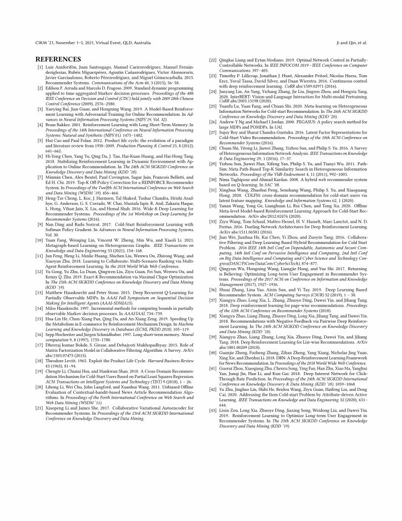
5.5 Hyperparameter Sensitivity AnalysisHere we also perform a sensitivity analysis for an important param-eter, the incorporation weight 𝛼 in Equation (7). Different choicesof 𝛼 generates different final score 𝑦, which similarly, can also havean NDCG evaluation introduced in Section 5.2. Furthermore, asan indication of CTR prediction with the true CTR label, AUC of

Figure 6: AUC, NDCG@10, NDCG@20 and NDCG@50curves with different 𝛼 . When more proportion of 𝑦𝑟𝑙 isadopted against 𝑦𝑐𝑡𝑟 , AUC decreases but NDCG of LTV in-creases, as expected.

𝑦 can also be evaluated with respect to different 𝛼 . As 𝛼 steadilychanges from 0 to 1, 𝑦 transforms from a ranking metric of CTRto a ranking metric of item LTV. By checking the curves of AUC(of CTR) and NDCG (of LTV) w.r.t. 𝛼 , one could have a snapshotabout the trade-off between the instant reward and the long-termreward. 3 The result is demonstrated in Figure 6. Not surprisingly,the AUC decreases while NDCG increases as 𝛼 increases. Basedon the shape of curves, we expect the mean of 𝛼 to be around 0.1where the AUC curve starts to decrease faster. Correspondingly,𝛼min and 𝛼max in Equation (8) are set to 0 and 0.2, respectively.

6 CONCLUSIONIn this paper, we propose a novel RL-LTV framework which solvesthe cold-start recommendation problem by considering the longer-term rewards of items, the LTVs. A special form of MDP, POC-MDP,is employed to model the item life dynamics. Generalized item-levelobservation and action spaces, as well as parameter-shared net-works, help the knowledge transfer from mature, historical itemsto fresh, cold-start items. An off-policy, actor-critic RL agent withan LSTM component is employed to interactively learn and changethe online system with a policy optimizing both instant rewardand long-term LTV. It is the first time to incorporate such poli-cies into the online recommendation system, to address the itemcold-start issue. We develop a training framework called IE-RDPGto complete the large scale, itemwise episodic training task. Byrigorous experiments, it shows that our algorithm performs muchbetter on the long-term rewards of cold-start items, comparingwith the online state-of-the-art baseline on Taobao. There is noevident degradation of the entire online performance during theexperiment. For future work, it would be interesting to use RL tostudy the entire life periods of products, therefore produce policiesnot only for cold-start but also lifelong recommendation. Anotherpossible improvement is to make the model more explainable toexplicitly exhibit the lifetime stage transitions of products.

3Note 𝛼 should vary with different items according to Equation (8). However, here wejust perform a simplified offline analysis by fixing all items with the same 𝛼 .


REFERENCES[1] Luis Anidorifón, Juan Santosgago, Manuel Caeirorodríguez, Manuel Fernán-

deziglesias, Rubén Míguezpérez, Agustin Cañasrodríguez, Victor Alonsororís,Javier Garcíaalonso, Roberto Pérezrodríguez, and Miguel Gómezcarballa. 2015.Recommender Systems. Communications of the Acm 40, 3 (2015), 56–58.

[2] Edilson F. Arruda and Marcelo D. Fragoso. 2009. Standard dynamic programmingapplied to time aggregated Markov decision processes. Proceedings of the 48hIEEE Conference on Decision and Control (CDC) held jointly with 2009 28th ChineseControl Conference (2009), 2576–2580.

[3] Xueying Bai, Jian Guan, and Hongning Wang. 2019. A Model-Based Reinforce-ment Learning with Adversarial Training for Online Recommendation. In Ad-vances in Neural Information Processing Systems (NIPS’19, Vol. 32).

[4] Bram Bakker. 2001. Reinforcement Learning with Long Short-Term Memory. InProceedings of the 14th International Conference on Neural Information ProcessingSystems: Natural and Synthetic (NIPS’01). 1475–1482.

[5] Hui Cao and Paul Folan. 2012. Product life cycle: the evolution of a paradigmand literature review from 1950–2009. Production Planning & Control 23, 8 (2012),641–662.

[6] Hi-Yong Chen, Yang Yu, Qing Da, J. Tan, Hai-Kuan Huang, and Hai-Hong Tang.2018. Stabilizing Reinforcement Learning in Dynamic Environment with Ap-plication to Online Recommendation. In The 24th ACM SIGKDD Conference onKnowledge Discovery and Data Mining (KDD ’18).

[7] Minmin Chen, Alex Beutel, Paul Covington, Sagar Jain, Francois Belletti, andEd H. Chi. 2019. Top-K Off-Policy Correction for a REINFORCE RecommenderSystem. In Proceedings of the Twelfth ACM International Conference on Web Searchand Data Mining (WSDM ’19). 456–464.

[8] Heng-Tze Cheng, L. Koc, J. Harmsen, Tal Shaked, Tushar Chandra, Hrishi Arad-hye, G. Anderson, G. S. Corrado, W. Chai, Mustafa Ispir, R. Anil, Zakaria Haque,L. Hong, Vihan Jain, X. Liu, and Hemal Shah. 2016. Wide & Deep Learning forRecommender Systems. Proceedings of the 1st Workshop on Deep Learning forRecommender Systems (2016).

[9] Nan Ding and Radu Soricut. 2017. Cold-Start Reinforcement Learning withSoftmax Policy Gradient. In Advances in Neural Information Processing Systems,Vol. 30.

[10] Yuan Fang, Wenqing Lin, Vincent W. Zheng, Min Wu, and Xiaoli Li. 2021.Metagraph-based Learning on Heterogeneous Graphs. IEEE Transactions onKnowledge and Data Engineering 33 (2021), 154–168.

[11] Jun Feng, Heng Li, Minlie Huang, Shichen Liu, Wenwu Ou, Zhirong Wang, andXiaoyan Zhu. 2018. Learning to Collaborate: Multi-Scenario Ranking via Multi-Agent Reinforcement Learning. In the 2018 World Wide Web Conference.

[12] Yu Gong, Yu Zhu, Lu Duan, Qingwen Liu, Ziyu Guan, Fei Sun, Wenwu Ou, andKenny Q. Zhu. 2019. Exact-K Recommendation via Maximal Clique Optimization.In The 25th ACM SIGKDD Conference on Knowledge Discovery and Data Mining(KDD ’19).

[13] Matthew Hausknecht and Peter Stone. 2015. Deep Recurrent Q-Learning forPartially Observable MDPs. In AAAI Fall Symposium on Sequential DecisionMaking for Intelligent Agents (AAAI-SDMIA15).

[14] Milos Hauskrecht. 1997. Incremental methods for computing bounds in partiallyobservable Markov decision processes. In AAAI/IAAI. 734–739.

[15] Hua-Lin He, Chun-Xiang Pan, Qing Da, and An-Xiang Zeng. 2019. Speeding Upthe Metabolism in E-commerce by Reinforcement Mechanism Design. InMachineLearning and Knowledge Discovery in Databases (ECML PKDD 2018). 105–119.

[16] Sepp Hochreiter and Jürgen Schmidhuber. 1997. Long short-termmemory. Neuralcomputation 9, 8 (1997), 1735–1780.

[17] Dheeraj kumar Bokde, S. Girase, and Debajyoti Mukhopadhyay. 2015. Role ofMatrix Factorization Model in Collaborative Filtering Algorithm: A Survey. ArXivabs/1503.07475 (2015).

[18] Theodore Levitt. 1965. Exploit the Product Life Cycle. Harvard Business Review43 (1965), 81–94.

[19] Chengte Li, Chiatai Hsu, and Mankwan Shan. 2018. A Cross-Domain Recommen-dation Mechanism for Cold-Start Users Based on Partial Least Squares Regression.ACM Transactions on Intelligent Systems and Technology (TIST) 9 (2018), 1 – 26.

[20] Lihong Li, Wei Chu, John Langford, and Xuanhui Wang. 2011. Unbiased OfflineEvaluation of Contextual-bandit-based News Article Recommendation Algo-rithms. In Proceedings of the Forth International Conference on Web Search andWeb Data Mining (WSDM ’11).

[21] Xiaopeng Li and James She. 2017. Collaborative Variational Autoencoder forRecommender Systems. In Proceedings of the 23rd ACM SIGKDD InternationalConference on Knowledge Discovery and Data Mining.

[22] Qingkai Liang and Eytan Modiano. 2019. Optimal Network Control in Partially-Controllable Networks. In IEEE INFOCOM 2019 - IEEE Conference on ComputerCommunications. 397–405.

[23] Timothy P. Lillicrap, Jonathan J. Hunt, Alexander Pritzel, Nicolas Heess, TomErez, Yuval Tassa, David Silver, and Daan Wierstra. 2016. Continuous controlwith deep reinforcement learning. CoRR abs/1509.02971 (2016).

[24] Junyang Lin, An Yang, Yichang Zhang, Jie Liu, Jingren Zhou, and Hongxia Yang.2020. InterBERT: Vision-and-Language Interaction for Multi-modal Pretraining.CoRR abs/2003.13198 (2020).

[25] Yuanfu Lu, Yuan Fang, and Chuan Shi. 2020. Meta-learning on HeterogeneousInformation Networks for Cold-start Recommendation. In The 26th ACM SIGKDDConference on Knowledge Discovery and Data Mining (KDD ’20).

[26] Andrew Y Ng and Michael I Jordan. 2000. PEGASUS: A policy search method forlarge MDPs and POMDPs. In UAI.

[27] Sujoy Roy and Sharat Chandra Guntuku. 2016. Latent Factor Representations forCold-Start Video Recommendation. Proceedings of the 10th ACM Conference onRecommender Systems (2016).

[28] Chuan Shi, Yitong Li, Jiawei Zhang, Yizhou Sun, and Philip S. Yu. 2016. A Surveyof Heterogeneous Information Network Analysis. IEEE Transactions on Knowledge& Data Engineering 29, 1 (2016), 17–37.

[29] Yizhou Sun, Jiawei Han, Xifeng Yan, Philip S. Yu, and Tianyi Wu. 2011. Path-Sim: Meta Path-Based Top-K Similarity Search in Heterogeneous InformationNetworks. Proceedings of the Vldb Endowment 4, 11 (2011), 992–1003.

[30] Nima Taghipour and Ahmad Kardan. 2008. A hybrid web recommender systembased on Q-learning. In SAC ’08.

[31] Xinghua Wang, Zhaohui Peng, Senzhang Wang, Philip S. Yu, and XiaoguangHong. 2020. CDLFM: cross-domain recommendation for cold-start users vialatent feature mapping. Knowledge and Information Systems 62, 1 (2020).

[32] Yanan Wang, Yong Ge, Lianghuan Li, Rui Chen, and Tong Xu. 2020. OfflineMeta-level Model-based Reinforcement Learning Approach for Cold-Start Rec-ommendation. ArXiv abs/2012.02476 (2020).

[33] Ziyu Wang, Tom Schaul, Matteo Hessel, H. V. Hasselt, Marc Lanctot, and N. D.Freitas. 2016. Dueling Network Architectures for Deep Reinforcement Learning.ArXiv abs/1511.06581 (2016).

[34] Jian Wei, Jianhua He, Kai Chen, Yi Zhou, and Zuoyin Tang. 2016. Collabora-tive Filtering and Deep Learning Based Hybrid Recommendation for Cold StartProblem. 2016 IEEE 14th Intl Conf on Dependable, Autonomic and Secure Com-puting, 14th Intl Conf on Pervasive Intelligence and Computing, 2nd Intl Confon Big Data Intelligence and Computing and Cyber Science and Technology Con-gress(DASC/PiCom/DataCom/CyberSciTech), 874–877.

[35] Qingyun Wu, Hongning Wang, Liangjie Hong, and Yue Shi. 2017. Returningis Believing: Optimizing Long-term User Engagement in Recommender Sys-tems. Proceedings of the 2017 ACM on Conference on Information and KnowledgeManagement (2017), 1927–1936.

[36] Shuai Zhang, Lina Yao, Aixin Sun, and Yi Tay. 2019. Deep Learning BasedRecommender System. ACM Computing Surveys (CSUR) 52 (2019), 1 – 38.

[37] Xiangyu Zhao, Long Xia, L. Zhang, Zhuoye Ding, Dawei Yin, and Jiliang Tang.2018. Deep reinforcement learning for page-wise recommendations. Proceedingsof the 12th ACM Conference on Recommender Systems (2018).

[38] Xiangyu Zhao, Liang Zhang, Zhuoye Ding, Long Xia, Jiliang Tang, and Dawei Yin.2018. Recommendations with Negative Feedback via Pairwise Deep Reinforce-ment Learning. In The 24th ACM SIGKDD Conference on Knowledge Discoveryand Data Mining (KDD ’18).

[39] Xiangyu Zhao, Liang Zhang, Long Xia, Zhuoye Ding, Dawei Yin, and JiliangTang. 2018. Deep Reinforcement Learning for List-wise Recommendations. ArXivabs/1801.00209 (2018).

[40] Guanjie Zheng, Fuzheng Zhang, Zihan Zheng, Yang Xiang, Nicholas Jing Yuan,Xing Xie, and Zhenhui Li. 2018. DRN: ADeep Reinforcement Learning Frameworkfor News Recommendation. In Proceedings of the 2018WorldWideWeb Conference.

[41] Guorui Zhou, Xiaoqiang Zhu, Chenru Song, Ying Fan, Han Zhu, XiaoMa, YanghuiYan, Junqi Jin, Han Li, and Kun Gai. 2018. Deep Interest Network for Click-Through Rate Prediction. In Proceedings of the 24th ACM SIGKDD InternationalConference on Knowledge Discovery & Data Mining (KDD ’18). 1059–1068.

[42] Yu Zhu, Jinghao Lin, Shibi He, Beidou Wang, Ziyu Guan, Haifeng Liu, and DengCai. 2020. Addressing the Item Cold-start Problem by Attribute-driven ActiveLearning. IEEE Transactions on Knowledge and Data Engineering 32 (2020), 631–644.

[43] Lixin Zou, Long Xia, Zhuoye Ding, Jiaxing Song, Weidong Liu, and Dawei Yin.2019. Reinforcement Learning to Optimize Long-term User Engagement inRecommender Systems. In The 25th ACM SIGKDD Conference on KnowledgeDiscovery and Data Mining (KDD ’19).