Reducing Parameter Uncertainty for Stochastic Systems∗

Szu Hui NG† Stephen E. CHICK‡

November 21, 2005

Abstract

The design of many production and service systems is informed by stochastic model analy-sis. But the parameters of statistical distributions of stochastic models are rarely known withcertainty, and are often estimated from field data. Even if the mean system performance is aknown function of the model’s parameters, there may still be uncertainty about the mean per-formance because the parameters are not known precisely. Several methods have been proposedto quantify this uncertainty, but data sampling plans have not yet been provided to reduceparameter uncertainty in a way that effectively reduces uncertainty about mean performance.The optimal solution is challenging, so we use asymptotic approximations to obtain closed-formresults for sampling plans. The results apply to a wide class of stochastic models, includingsituations where the mean performance is unknown but estimated with simulation. Analyticaland empirical results for the M/M/1 queue, a quadratic response-surface model, and a simulatedcritical care facility illustrate the ideas.

Category: G.3: Probability and Statistics, Probabilistic algorithms (including Monte Carlo)experimental design

Category: I.6: Simulation and Modeling, Simulation output analysisTerms: Experimentation, PerformanceKeywords: Stochastic simulation, uncertainty analysis, parameter estimation, Bayesian statis-

tics

1 Introduction

Stochastic modeling and simulation analysis are useful approaches to evaluate the performance ofproduction and service systems as a function of design and statistical parameters [e.g., Buzacott andShanthikumar 1993; Law and Kelton 2000]. Models of existing systems, or variations of existingsystems, can help inform system design and improvement decisions. Data may be available tohelp estimate statistical parameters, but estimators are subject to random variation because theyare functions of random phenomena. Parameter uncertainty means that there is a risk that aplanned system will not perform as expected [Cheng and Holland 1997; Chick 1997, 2001; Bartonand Schruben 2001], even if the relationship between the parameters and system performance is

∗ c©ACM, (2006). This is the author’s version of the work. It is posted here by permission of ACM for yourpersonal use. Not for redestribution. The definitive version was published in ACM TOMACS {Vol 16, Iss 1, Jan.2006}. http://www.linklings.net/tomacs/index.html

†S.-H. Ng, Dept. Industrial and Systems Engineering, National University of Singapore, 10 Kent Ridge Crescent,Singapore 119260, isensh@nus.edu.sg.

‡S. E. Chick, Technology and Operations Management Area, INSEAD, Boulevard de Constance, 77305Fontainebleau CEDEX, France, stephen.chick@insead.edu.

1

completely known. For example, the stationary mean occupancy of a stable M/M/1 queue is aknown function of the arrival and service rates, but the mean occupancy is unknown if those ratesare not precisely known. When the system performance is an unknown function of the parameters,and is estimated by simulation, the problem is aggravated. The common practice of inputtingpoint estimates of parameters into simulations can dramatically reduce the coverage of a supposedly100(1− α)% confidence interval (CI) for the mean performance (Barton and Schruben 2001).

Bootstrap methods (Cheng and Holland 1997; Barton and Schruben 2001), asymptotic normal-ity approximations (Cheng and Holland 1997; Ng and Chick 2001), and Bayesian model averaging[Draper 1995; Chick 2001; Zouaoui and Wilson 2003, 2004] can quantify the effect of input param-eter uncertainty on output uncertainty.

This paper goes beyond quantifying uncertainty by suggesting how to reduce parameter uncer-tainty in a way that effectively reduces uncertainty about the mean performance of a system. Wedo so for a broad class of stochastic systems by using asymptotic variance approximations for theunknown mean system performance. Section 2 formalizes the stochastic model assumptions alongwith examples. Section 3 introduces the asymptotic variance approximations for input parameteruncertainty. Section 4 describes how input parameter uncertainty affects output uncertainty andformulates an optimization problem to reduce output uncertainty. When the system response isa known function of the inputs, the optimal sampling plan turns out to be very similar to knownresults for stratified sampling. When the system response must be estimated with simulation, adifferent sampling allocation is obtained. The allocation shows how to balance the cost of runningadditional simulations (to reduce uncertainty about the mean response and its gradient) and datacollection (to reduce uncertainty about the inputs to the system). Under some general conditions,the optimal sampling allocations are shown to have the attractive property of being invariant to thecoordinate systems used to represent the parameter of each input distribution. Section 5 appliesthe results to several examples. This paper extends preliminary work (Ng and Chick 2001) by gen-eralizing results to a broader class of distributions, and by providing results for unknown responsefunctions. An appendix also describes how to reduce the mean-squared error (MSE) rather thanthe variance. The approach taken is Bayesian, so parameter uncertainty is quantified with randomvariables.

2 Model Formulation and Examples

Consider a system with multiple statistical parameters Θ = (θ1, θ2, . . . ,θk) that influence thesystem performance g(Θ). Simulated performance realizations Yl (“output”) with input parameterΘl for replication l = 1, 2, . . .,

Yl = g(Θl) + σ(Θl)Zl,

may be observed if g(Θ) is unknown, where σ2 is the output variance, and the Zl are independentzero-mean random variables with unit variance.

The system is driven by k scalar (real-valued) input processes that are mutually independentsources of randomness. Given the parameter vector θi for the ith input process, the correspondingobservations {xi` : ` = 1, 2, . . .} are independent and identically distributed with conditional prob-ability density function pi(xi` | θi). Uncertainty about the parameter θi is initially described witha probability model πi(θi). In Bayesian statistics, πi(θi) is called a prior probability distribution.Here we presume joint independence across sources of randomness, π(Θ) =

∏ki=1 πi(θi).

Each θi is assumed to be inferrable from data. The data xi = (xi1, xi2, . . . , xini) that has beenobserved so far for the ith input process can be used to get a more precise idea about the value of

2

the unknown parameter θi, whose uncertainty is characterized by the posterior distribution

fini(θi | xi) ∝ πi(θi)ni∏

`=1

pi(xi` | θi), (1)

for i = 1, 2, . . . , k. We will use those distributions to figure out how to collect additional data, ifneeded, to reduce uncertainty about input parameters. Let n = (n1, . . . , nk) specify the numberof data points observed so far for each source of randomness. Probability statements below are allconditional on all data collected so far, En = (xT

1 , . . . , xTk ), unless otherwise specified.

A tilde denotes the maximum a posteriori (MAP) estimate of any parameter, e.g. θini maximizesfini . Maximum likelihood estimates (MLEs) are denoted with a hat, θini . Given the data xi, theMLE maximizes

∏ni`=1 pi(xi` | θi).

Parameters may be multivariate, such as θ1 = (ϑ1, ϑ2). It will be convenient at times to refer tothe individual components of the parameter vector Θ = (θ1, θ2, . . . , θk) encompassing all k sourcesof randomness; and for this purpose we write Θ = (ϑ1, ϑ2, . . . , ϑK), where K > k when at least oneof the θi are multidimensional. Decision variables and system control parameters are consideredto be fixed and implicit in the definition of g, so that we focus upon the effects of input parameteruncertainty. Table 1 summarizes this notation, as well as much of the notation used in the rest ofthe paper.

The M/M/1 queue can be described with this notation as a system with k = 2 sources ofrandomness (arrival and service times), with arrival rate θ1 = λ and service rate θ2 = µ. Thereare a total of K = 2 components of the overall parameter vector Θ, so Θ = (λ, µ). The stationarymean occupancy is known in closed form if the queue is stable, g(Θ) = λ/(µ− λ).

A less trivial example for which the system response is unknown is the critical care facilitydepicted in Figure 1. Schruben and Margolin (1978) studied that system to determine the expectednumber of patients per month that are denied a bed, as a function of the number of beds in theintensive care unit (ICU), coronary care unit (CCU), and intermediate care units. Patients arriveaccording to a Poisson process and are routed through the system depending upon their specifichealth condition. Their analysis presumed fixed point estimates (MLE) for the parameters of thek = 6 sources of randomness: the patient arrival process (Poisson arrivals, mean θ1n = 3.3/day),ICU stay duration (lognormal θ2 = (ϑ2, ϑ3), with mean ϑ2n = 3.4 and standard deviation ϑ3n = 3.5days), three more bivariate input parameters θ3, θ4, θ5 for the lognormal service times at theintermediate ICU, intermediate CCU, and CCU processes, and a sixth parameter for patient routing(multinomial, θ6n = (p1, p3, p4) = (.2, .2, .05), note that p2 = 1− p1 − p3 − p4). There are thereforea total of K = 12 components of the overall parameter vector Θ. The function g(·) is not known,and is to be estimated from simulation near the point Θn.

This paper will use approximations that assume a constant variance, σ(Θ) = σ (homoscedastic).If the variance actually depends upon Θ (heteroscedastic), then we will estimate σ by the MAPestimator σ(Θn), a Bayesian analog of the usual MLE for the standard deviation, σ(Θn). Thisapproximation is a standard assumption in the design of experiments literature (Box, Hunter, andHunter 1978; Box and Draper 1987; Myers, Khuri, and Carter 1989), and is asymptotically validunder certain conditions (Mendoza 1994, p. 176) if σ(Θ) is a “nice” function of Θ near Θn.

The approximations made below in a Bayesian context are analogous to frequentist approxi-mations by Cheng and Holland (1997). The modification of the analysis is with a straightforwardapplication of results of Bernardo and Smith (1994), and result in a decoupling of stochastic un-certainty from parameter uncertainty when g(·) is a known function. Zouaoui and Wilson (2001)used a similar decoupling to obtain a variance reduction for estimates of E[g(Θ) | En] with theBayesian Model Average (BMA) when multiple candidate distributions are proposed for a single

3

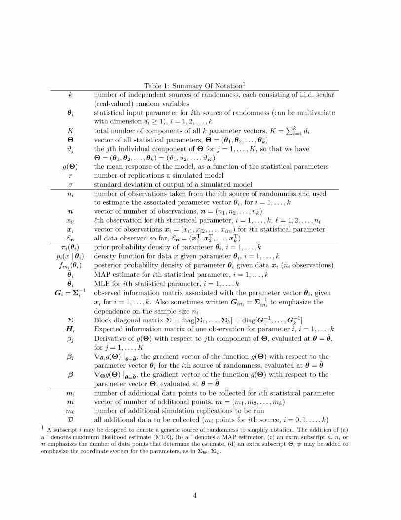
Table 1: Summary Of Notation1

k number of independent sources of randomness, each consisting of i.i.d. scalar(real-valued) random variables

θi statistical input parameter for ith source of randomness (can be multivariatewith dimension di ≥ 1), i = 1, 2, . . . , k

K total number of components of all k parameter vectors, K =∑k

i=1 di

Θ vector of all statistical parameters, Θ = (θ1, θ2, . . . ,θk)ϑj the jth individual component of Θ for j = 1, . . . ,K, so that we have

Θ = (θ1, θ2, . . . ,θk) = (ϑ1, ϑ2, . . . , ϑK)g(Θ) the mean response of the model, as a function of the statistical parameters

r number of replications a simulated modelσ standard deviation of output of a simulated modelni number of observations taken from the ith source of randomness and used

to estimate the associated parameter vector θi, for i = 1, . . . , kn vector of number of observations, n = (n1, n2, . . . , nk)xi` `th observation for ith statistical parameter, i = 1, . . . , k; ` = 1, 2, . . . , ni

xi vector of observations xi = (xi1, xi2, . . . , xini) for ith statistical parameterEn all data observed so far, En = (xT

1 , xT2 , . . . ,xT

k )πi(θi) prior probability density of parameter θi, i = 1, . . . , k

pi(x | θi) density function for data x given parameter θi, i = 1, . . . , kfini(θi) posterior probability density of parameter θi given data xi (ni observations)

θi MAP estimate for ith statistical parameter, i = 1, . . . , k

θi MLE for ith statistical parameter, i = 1, . . . , k

Gi = Σ−1i observed information matrix associated with the parameter vector θi, given

xi for i = 1, . . . , k. Also sometimes written Gini = Σ−1ini

to emphasize thedependence on the sample size ni

Σ Block diagonal matrix Σ = diag[Σ1, . . . ,Σk] = diag[G−11 , . . . , G−1

k ]H i Expected information matrix of one observation for parameter i, i = 1, . . . , k

βj Derivative of g(Θ) with respect to jth component of Θ, evaluated at θ = θ,for j = 1, . . . , K

βi ∇θig(Θ) |θ=θ, the gradient vector of the function g(Θ) with respect to theparameter vector θi for the ith source of randomness, evaluated at θ = θ

β ∇Θg(Θ) |θ=θ, the gradient vector of the function g(Θ) with respect to theparameter vector Θ, evaluated at θ = θ

mi number of additional data points to be collected for ith statistical parameterm vector of number of additional points, m = (m1, m2, . . . , mk)m0 number of additional simulation replications to be runD all additional data to be collected (mi points for ith source, i = 0, 1, . . . , k)

1 A subscript i may be dropped to denote a generic source of randomness to simplify notation. The addition of (a)a ˆ denotes maximum likelihood estimate (MLE), (b) a ˜ denotes a MAP estimator, (c) an extra subscript n, ni orn emphasizes the number of data points that determine the estimate, (d) an extra subscript Θ, ψ may be added toemphasize the coordinate system for the parameters, as in ΣΘ, Σψ.

4

Intensive Care Unit

(ICU)

Intermediate ICU

Coronary Care Unit

(CCU)

Intermediate CCU

Patient

Entry

Exit

Exit

Exit

Exit

0.20

0.55

0.20

0.05

Figure 1: Fraction of patients routed through different units of a critical care facility.

source of randomness, and the response is homoscedastic. Their result appears to be extendableto the heteroscedastic case (n → ∞) by approximating σ with σ(Θn). The idea of decouplingstochastic and parameter uncertainty is applied to the case of an unknown g(Θ) with an unknowngradient in Section 4.2.

3 Approximations for Parameter Uncertainty

Uncertainty about parameters, and the effect of data collection variability, is approximated by thevariance. The mean squared error (MSE) of estimates is treated in Appendix A. The analysis ismotivated by analogy with the following well-known result for confidence intervals based on asymp-totic normality. Suppose that the simulation outputs y1, . . . , yr are observed, with sample meanyr, sample variance S2

r , and 100(1− α)% CI for the mean yr ± tr−1,1−α/2(S2r/r)

12 . An approximate

expression for the number of additional observations m∗ required to obtain an absolute error of ε ism∗ = min

{m ≥ 0 : tr+m−1,1−α/2

[S2

r/(r + m)]1/2 ≤ ε

}. For large r, tr+m−1,1−α/2 does not change

much as a function of m. The CI width is essentially scaled by shrinking the variance for theunknown mean from S2

r/r toS2

r/(r + m). (2)

Analogous results exist for asymptotic normal approximations to the posterior distributions ofinput parameters.

For the rest of this section, we focus on one parameter θ = (ϑ1, . . . , ϑd) for a single source ofrandomness (dropping the subscript i for notational simplicity).

Proposition 3.1. For each n, let fn(·|xn) denote the posterior p.d.f. of the d-dimensional pa-rameter vector θn; let θn be the associated MAP; and define the Bayesian observed informationGn = Σ−1

n by

[Gn]jl =[Σ−1

n

]jl

= −∂2 log fn(θ | xn)∂ϑj∂ϑl

∣∣∣∣θ=θn

for j, l = 1, . . . , d. (3)

Then the random variable Σ−1/2n (θn − θn) converges in distribution to a standard (multivariate)

normal random variable as n →∞ if certain regularity conditions hold.

5

Proof. See Bernardo and Smith (1994, Prop 5.14). The regularity conditions presume a nonzeroprior probability density near the “true” θ, and the “steepness”, “smoothness”, and “concentration”regularity conditions imply that the data is informative for all components of θn, so the posteriorbecomes peaked near θn.

Colloquially, Σn is proportional to 1/n, so the posterior variance shrinks as in Equation (2)as additional samples are observed. Gelman, Carlin, Stern, and Rubin (1995, Sec. 4.3) describewhen the regularity conditions may not hold, including underspecified models, nonidentified param-eters, cases in which the number of parameters grows with the sample size, unbounded likelihoodfunctions, improper posterior distributions, or convergence to a boundary of the parameter space.

The expected information matrix in one observation is

[H(θn)]jl = EX`

[−∂2 log p(X` | θ)

∂ϑj∂ϑl

] ∣∣∣∣θ=θn

for j, l = 1, . . . , d.

so the analog to the asymptotic approximation in Equation (2) for the variance of θ, given that madditional data points are to be collected, is

(Σ−1n + mH(θn))−1. (4)

Equation (4) simplifies under some special conditions. A sufficient condition is that the distri-bution for θ be in the regular exponential family (which includes the exponential, gamma, normal,binomial, multinomial, lognormal, Poisson, and many other distributions) and that a conjugateprior distribution be used to describe initial parameter uncertainty (see Appendix B). Use of aconjugate prior distribution implies that the posterior distribution will have the same functionalform as the prior distribution.

Appendix B shows that if the prior distribution before observing any data is a conjugate prior,then Σ−1

n = (n0 + n)H(θn) for some n0 and Equation (4) simplifies:

(Σ−1n + mH(θn))−1 =

H−1(θn)n0 + n + m

. (5)

Equation (4) also simplifies if the MLE θn replaces θn and the expected information Σ−1n = nH(θn)

replaces Σ−1n .

All of the distributions for the M/M/1 queue and the critical care facility are in the regularexponential family and satisfy the regularity conditions of Proposition 3.1. The specific numbersof service time and routing decision observations for the critical care facility were not published.For the analysis here, we presumed standard noninformative prior distributions for each unknownparameter (Bernardo and Smith 1994). We further assumed that the published point estimateswere MLEs based on 100 patients, so that 20 patients were routed to the ICU alone, 5 were routedto the CCU alone, and so forth. This assumption uniquely determines the sufficient statistics ofthe data and the proper posterior distributions for the parameters. It also uniquely determines theobserved information matrices Σ−1

n for each parameter. Ng and Chick (2001) provided details forthe information matrix and input uncertainty of the Poisson and lognormal distributions. For themultinomial routing probabilities, the Dirichlet distribution is the conjugate prior, π(p1, p3, p4) ∝pα01−11 pα03−1

3 pα04−14 (1 − p1 − p3 − p4)α02−1, with noninformative distribution α0j = 1/2 for j =

1, . . . , 4 (Bernardo and Smith 1994). Reparametrizing this into the canonical conjugate form as inAppendix B, we have ψ = (log p1, log p3, log p4). Since this mapping is bijective, the results fromAppendix B also hold in the (p1, p3, p4) coordinates. If sj patients are routed to location j, then the

6

posterior distribution is Dirichlet with parameters αj = α0j+sj . If αj > 1 for all j, then the MAP ispj = (αj−1)/[

∑4j=1(αj−1)], and Σ−1

n = [∑4

j=1(αj−1)]H(θn) = [42 +n−4]H(θn) = (n0+n)H(θn),where n0 = −2.

4 Parameter and Performance Uncertainty

Section 4.1 derives approximations for performance uncertainty, measured by variance, as a functionof parameter uncertainty when g(·) is a known function. It formulates and solves an optimizationproblem that allocates resources for further data collection to minimize an asymptotic approxima-tion to performance uncertainty. Section 4.2 identifies sampling allocations when g(·) is unknown.It shows whether it is more important to run more simulation replications (to improve the gradientestimate) or to collect more field data (to reduce parameter uncertainty).

4.1 Known Response Function

Denote gradient information of the known response surface, g(Θ), evaluated at the MAP estimatorof Θ, by

βj =∂g(Θ)∂ϑj

∣∣∣∣Θ=Θn

for j = 1, . . . , K (6)

βi = ∇θig(Θ)∣∣∣∣Θ=Θn

for i = 1, . . . , k

β = (β1, β2, . . . , βk).

Suppose that the parameters for each source of randomness are estimated with n observations each,and that each satisfies the asymptotic normality properties of Proposition 3.1. Proposition 4.1 statesthat g(Θ) is also asymptotically normal as more observations are collected from each of the sourcesof randomness.

Proposition 4.1. Use the assumptions, notation and technical conditions of Proposition 3.1, withthe modification that Θn = (θ1n, . . . ,θkn) is the nth vector of parameters, so that fin(·) is the poste-rior density function of the random variable θin, the MAP estimator of Θ is Θn = (θ1n, . . . , θkn),and Σn = diag [Σ1n . . .Σkn] is the nth block diagonal matrix with appropriate submatrices forparameters i = 1, . . . , k, assuming n observations are available from each source of randomness.Suppose that Θ has an asymptotic Normal

(Θn,Σn

)distribution, as in the conclusion of Propo-

sition 3.1. Suppose that g is continuously differentiable near Θ0, that σ2n → 0 and Θn → Θ0 in

probability, and σ2n = O(σ2

n), where σ2n and σ2

n respectively denote the largest and smallest eigen-values of Σn.

The random variable (βnΣnβTn )−1/2[g(Θ) − g(Θn)] converges in distribution to the standard

normal distribution. Colloquially, g(Θ) is asymptotically distributed

Normal(g(Θn), βnΣnβT

n

).

Proof. Mendoza (1994) and Bernardo and Smith (1994, Prop. 5.17) provide an analogous result forbijective functions g(Θ) when k = 1. The result holds for univariate g(Θ) because the marginaldistribution of a single dimension of a multivariate joint Gaussian is also Gaussian. That resultgeneralizes directly to k ≥ 1, as required here, with straightforward algebra. This is a Bayesiananalog for classical results from Serfling (1980, Sec. 3.3).

7

Block diagonality reflects an assumption that the parameters for different sources of randomnessare a priori independent, and that samples are conditionally independent, given the value of Θ.

The plug-in estimator g(Θn) converges to g(Θ0) but is biased for nonlinear functions. Ap-pendix A discusses bias and the mean squared error of estimates, using a first-order bias approxi-mation. For now we focus on the variance of the estimators.

The number of observations for each of the k sources of randomness may differ, as may thenumber of additional data points to collect. Let ni be the number of data points for source i,suppose that mi additional points are to be collected for each source of randomness i, and setm = (m1, . . . , mk). Using the approximation of Equation (4), we see that the variance in theunknown performance after collecting additional information is approximately

Vpar(m) =k∑

i=1

βini(Σ−1ini

+ miH i(θini))−1βini

T (7)

If each observed information matrix is proportional to the corresponding expected informationmatrix, as when conjugate priors are used, then Equation (7) simplifies:

Vpar(m) =k∑

i=1

ξi

n0i + ni + mi, where ξi = βiniH

−1i (θini)βini

T . (8)

The optimal sampling plan for reducing this asymptotic approximation to the variance in systemperformance, assuming that sampling costs for source i is linear in the number of samples, istherefore the solution to Problem (9).

min Vpar(m) (9)s.t. mi ≥ 0 for i = 1, . . . , k∑

cimi = B

Cost differences may arise if data collection can be automated for some but not all sources ofrandomness, if suppliers differ in willingness to share data, and so forth.

Proposition 4.2. If Vpar(m) simplifies to Equation (8), the integer restriction is relaxed (contin-uous mi), and B is large, then the solution to Problem (9) is:

m∗i =

B +∑k

`=1(n0` + n`)c`

∑kj=1

(ξjcicj

ξi

)1/2− (n0i + ni) for i = 1, . . . , k (10)

Proof. See Appendix C.

For small B, the nonnegativity constraints for the mi need consideration. Special features ofthe data collection process can be handled by adding constraints, e.g. set a subset of mi’s to beequal for simultaneously reported data.

Example: The mean occupancy of an M/M/1 queue is g(λ, µ) = λ/(µ− λ) when µ > λ. Thegamma distribution is the conjugate prior for an unknown rate of samples with an exponentialdistribution. Suppose that a gamma prior distribution Gamma (α, ν) models uncertainty for theunknown arrival rate, with mean α/ν and density fΛ(w) = ναwα−1 exp(−wν)/Γ(α) for all w ≥ 0.If na arrivals are observed, the posterior distribution is also Gamma with parameters αλ = α +na, νλ = ν +

∑nal=1 xil. The MAP estimate is λ = (αλ − 1)/νλ, and H1(λ) = 1/λ2 = ν2

λ/(αλ − 1)2.

8

With calculus, Σ−11na

= (αλ − 1)/λ2 = ν2λ/(αλ − 1). Similarly assume the service rate has a

conjugate gamma prior, that ns service times are observed, resulting in a Gamma (αµ, νµ) posteriordistribution. If µ > λ (otherwise, we would consider a multiserver system), then Equation (7)implies

Vpar(m) =λ2µ2

(µ− λ)4

(1

αλ − 1 + ma+

1αµ − 1 + ms

).

As conjugate priors are used, Σ−11na

= (αλ− 1)H1(λna) and Σ−12ns

= (αµ− 1)H2(µns). This reducesto Equation (8) where n0a + na = αλ − 1 and n0s + ns = αµ − 1.

If ma interarrival times can be collected at cost ca each, and ms service times can be collectedat cost cs each, then by Proposition 4.2, it is optimal to sample with m∗

s = (B − cam∗a)/cs and

m∗a =

B + (αλ − 1)ca + (αµ − 1)cs

ca + (cacs)1/2− (αλ − 1)

for large B. If ca = cs, this choice minimizes the difference between αλ + ma and αµ + ms (thesame effective number of data points is desired for both parameters).

If the arrival and service rates are believed to have a gamma distribution, then the queue isunstable with positive probability. In fact, the expectation of the average queue length does notexist even after conditioning on stability, Eλ,µ[λ/(µ − λ) | λ < µ] = ∞ (Chick 2001). This meansthat using Bayesian models for unknown statistical input parameters may lead to simulation outputprocesses whose expectation is not defined. At least two alternative approaches can be taken. First,a similar analysis can be done for a model that not only has finite moments but is also more realistic(say, by considering a finite waiting capacity or by modeling a finite time horizon rather than aninfinite horizon time average). Second, one can use the asymptotic normality approximation in spiteof the lack of moments as a starting point for reducing input uncertainty. Section 5.2 illustrates byexample when this second alternative might be expected to work well or not.

The optimal allocation for Problem (9) does not depend on the parametrization Θ under cer-tain conditions. Let T : RK 7→ RK be a one-to-one continuously differentiable transformationψ = (ψ1, . . . , ψK) = T (Θ) = [T1(Θ), . . . , TK(Θ)] with differentiable inverse Θ = T−1(ψ), andnonsingular matrix of derivatives JT (Θ), where [JT (Θ)]j` = ∂Tj/∂ϑ`. We write JT−1(ψ), where[JT−1(ψ)]j` = ∂T−1

j /∂ψ`. Let ψn be the MAP estimator for ψ given En. Denote the response gra-dient with respect to ψ by βψ and the gradient in Equation (6) with respect to Θ by βΘ. Similarlydenote the observed information matrix and expected information in one observation (measuredin ψ coordinates) by Σψ,n and Hψ to emphasize the coordinate system. The expression Vpar(m)in Equation (8) explicitly depends upon Θ. We write Vpar(m;Θ) to denote that dependence ex-plicitly. Let Vpar(m;ψ) denote the analogous approximation approximation when computed in ψcoordinates.

Proposition 4.3. Suppose the setup of Proposition 4.1, that the distribution of Θ is in the regularexponential family, and that a conjugate prior is adopted. Let T : RK 7→ RK be a one-to-onecontinuously differentiable transformation ψ = T (Θ) = [T1(Θ), . . . , TK(Θ)] with differentiableinverse Θ = T−1(ψ), and nonsingular Jacobian JT (Θ). If conditions (a) for each i, ψi = Ti(Θ)depends upon only one θj, and (b) ψn = T (Θn) are true, then Vpar(m;Θ) = Vpar(m; ψ).

Proof. Presume the setup of Proposition 4.1, define T and the other notation as in the problemstatement, and suppose conditions (a) and (b) hold. Condition (a) means that JT (Θ) has thesame block diagonal structure as Σ, and that no ψi is a function of parameter vectors for multiplesources of randomness.

9

Suppose first that there is only k = 1 source of randomness with parameter θ and drop thesubscript i for notational simplicity. In this notation, ξi can be rewritten ξ = βΘH−1

Θ (Θn)βΘT in

Θ coordinates. By the chain rule for partial differentiation, and the assumption ψn = T (Θn),

βψ = ∇ψg(ψ)∣∣ψ=ψn

=(∇Θg(Θ)

∣∣Θ=Θn

)(JT−1(ψn)

).

By Schervish (1995, p. 115), Hψ(ψ) = JTT−1(ψ)HΘ(Θ)JT−1(ψ), so that with additional calculus

H−1ψ (ψ) = (JT

T−1(ψ)HΘ(Θ)JT−1(ψ))−1 = JT (Θ)H−1Θ (Θ)JT

T (Θ). Therefore, in ψ coordinates,

ξ = βψH−1ψ (ψn)βψ

T

= [∇Θg(Θn)JT−1(ψn)][JT (Θn)H−1Θ (Θn)JT

T (Θn)][JTT−1(ψn)∇T

Θg(Θn)]

= ∇Θg(Θn)H−1Θ (Θn)∇T

Θg(Θn)= βΘH−1

Θ (Θn)βΘT.

The third equality follows because JT (Θn)JT−1(ψn) = JT−1(ψn)JT (Θn) is the K ×K identitymatrix, when ψn = T (Θn) holds.

For k > 1, the block diagonality assumption of Condition (a) assures that the ξi decouple, onefor each of the k independent sources of randomness.

The MAP estimator is not invariant to coordinate changes. That is, if Θn is the MAP in Θcoordinates, and ψn is the MAP in ψ coordinates, then it may not be true that ψn = T (Θn). Forexample, if the unknown rate ψ of an exponential distribution has a Gamma (αn, νn) distribution,then ψn = (αn − 1)/νn and the mean θ = 1/ψ has an inverted gamma distribution, with MAPθn = νn/(αn + 1) 6= 1/ψn. The multivariate generalization of Proposition 4.1 implies that ψn andT (Θn) are asymptotically equal. For a Bayesian, then, the allocations are asymptotically invariantto parametrization, in this sense.

For a frequentist, the allocations are invariant for finite n, as the MLE is invariant, given mildregularity conditions (Edwards 1984), and expected information matrices behave as required for adevelopment parallel to Proposition 4.3.

4.2 Unknown Response Function

If the response function g(Θ) is unknown, an approximation is needed to estimate the mean ofsome future output Yr+1. The asymptotic approximations above “hit their limit” in some sensewith linear approximations, so we approximate g(Θ) near Θn with a first-order regression modelthat may depend on past simulation output.

E[Yr+1 | Θ] ≈ h(Θ, β) = β0 +K∑

j=1

βj(ϑj − ϑj) (11)

The notation h(Θ,β) replaces the notation g(Θ) to make it explicit that the estimated responsedepends upon both Θ and β. Note that β0 takes the role of g(Θ) and βj takes the role of ∂g(Θ)/∂ϑj .If the derivatives βj = ∂h/∂ϑj are estimated from simulations, for j = 1, 2, . . . ,K, then uncertaintyabout both Θ and β must be considered. We take a Bayesian approach and presume β to be arandom vector, whose posterior distribution is updated when simulation replications are run.

10

Suppose that r replications have been run, with r×(K+1) design matrix M = [(Θ1−Θn), (Θ2−Θn), . . . , (Θr − Θn)]T , resulting in outputs y = [y1, . . . , yr]T with sample mean y = r−1

∑ri=1 yi.

The r runs may have come from q replications at each of t design points selected with classicaldesign of experiments (DOE) techniques, with r = qt. Or the Θi may have come from using aBMA to sample t values of Θi independently from f(Θ | x), with q replications for each Θi (Chick(2001) used q = 1, Zouaoui and Wilson (2003) extended to q > 1 to assess stochastic uncertainty,also see Zouaoui and Wilson (2004)). In either case, the posterior distribution of β, assuming thestandard linear model with a noninformative prior distribution p(β, σ2) ∝ σ−2, and that r > (K+1)(Gelman, Carlin, Stern, and Rubin 1995, Sec. 8.3), is

p(β | y,M, σ2) ∼ Normal(βr, (M

TM)−1σ2)), (12)

p(σ2 | y,M) ∼ Inverse-Chi2(r − (K + 1), s2

),

βr = (β0, β1, β2, . . . , βk) = (MTM)−1MT y

s2 =1

r − (K + 1)(y −Mβr)

T (y −Mβr).

The standard classical estimate for β is βr, and for σ2 is s2.The posterior marginal distribution of β is actually multivariate t, not normal. We approxi-

mate this distribution by estimating σ2 by s2 and presuming the variance is known, as we did inEquation (2), to arrive at a normal distribution approximation for the unknown response vectorthat has mean βr and variance of the form Σβ/(r0 + r). Similarly, we presume that the poste-rior variance of β is of the form Σβ/(r0 + r + m0) when m0 additional replications are run (cf.Equation (8)). Amongst other scenarios, this approximation makes sense when m0 = q′t, with q′

additional replications are run at each of the t originally selected Θi as above.Then the approximation Vtot = Var(h(Θ, β) | En,y,M, σ2 = s2) for overall performance un-

certainty Var(E[Yr+1] | En, y,M) asymptotically consists of components that reflect parameteruncertainty (Vpar), response surface/gradient uncertainty (Vresp), and stochastic noise (σ2 = s2).The following expectations, through Equation (13), implicitly condition on all observations so far,En, y,M.

Vtot ≈ s2

r0 + r+

K∑

i=1

K∑

j=1

E{[

βi(ϑi − ϑi)(ϑj − ϑj)T βj

]

−E[βi(ϑi − ϑi)

]E

[βj(ϑj − ϑj)

]}

=s2

r0 + r+

K∑

i=1

K∑

j=1

E [βiβj ] Cov(ϑi, ϑj)

=s2

r0 + r+

K∑

i=1

K∑

j=1

Cov(ϑi, ϑj) [E(βi)E(βj) + Cov(βi, βj)]

≈ s2

r+

k∑

i=1

∇θih(Θn, βr)Σini∇θih(Θn, βr)T

+K∑

i=1

K∑

j=1

[Σβ]ijr

[Σn]ij

def= Vstoch + Vpar + Vresp (13)

11

The last equality defines Vresp. The preceding equalities depend upon independence and asymp-totic normality assumptions. The term Vstoch = s2/r in the second approximation (with r0 = 0)follows directly from plugging in s2 for σ2 and examining the posterior conditional variance of β0

in Equation (12). Cheng and Holland (2004) also found an estimator of Vstoch that is proportionalto 1/r.

Cheng and Holland (2004) describe several methods to estimate the gradients of a stochasticsimulation model with an unknown response model, and use those results to approximate Vstoch andVpar. A full study of the merits of the many ways to estimate the gradient β, and their influenceupon Vtot, is an area for further study.

Since Cov(βi, βj) is inversely proportional to the number of runs, the asymptotic approximationfor all uncertainty if m0 more replications and mi data samples for each input are collected can beapproximated (cf. Equation (8)) by

Vtot(m,m0) =s2

r + m0+

k∑

i=1

ξi

n0i + ni + mi+

ai

(r + m0)(n0i + ni + mi), (14)

where ai represents the sum of the subset of the terms in∑K

l=1

∑Kj=1[Σβ]lj

[H−1

n

]lj

that have bothl and j indexing components of the overall parameter vector that deal with θi, for i = 1, . . . , k.The double sum decouples into one term per input parameter vector due to the block diagonalityof Σn. Derivatives confirm that Vtot(m,m0) is convex and decreasing in m0 and each mi.

Suppose there is a sampling constraint for more field data and simulation runs,

B = c0m0 +k∑

i=1

cimi.

By Proposition 4.2, the m that minimizes Vtot(m,m0) for a fixed m0 < B/c0, subject to thesampling constraint, can be found by substituting B with B − c0m0, and replacing ξi with ξi +ai/(r + m0) for i = 1, 2, . . . , k in Equation (10). The optimal (m,m0) can then be found byunivariate search for the optimal m0. In practice, one might run more replications if Vstoch + Vresp

is large relative to Vpar(m), and do more data collection if Vpar(m) is unacceptably large.

5 Experimental Analysis

This section presents numerical studies to assess how close the asymptotic approximations are tothe actual variance. It also assesses the variance, bias, and root mean squared error (RMSE)of estimators of the unknown mean performance as a function of both the number of initiallycollected samples of data and the total number of additional samples to be collected. We evaluatethe influence of response surface uncertainty for a quadratic response in Section 5.1, consider aknown nonlinear function with unknown parameters in Section 5.2, and apply the ideas to theICU simulation in Section 5.3. In all three examples, we assume noninformative prior distributionsfor the unknown parameters, and initial data collection is complemented with a follow-up datacollection plan based upon Equation (7) or Equation (14).

5.1 Unknown Nonlinear Response

The first numerical experiment assesses the reduction in uncertainty about the mean performanceassuming that the response surface is unknown. Assume that the unknown parameters are themean µi and precision λi of k = 3 sources of randomness for which data xi` has been observed

12

(i = 1, 2, 3; ` = 1, 2, . . . , ni). The response function is quadratic in Θ = (µ1, λ1, µ2, λ2, µ3, λ3), withknown functional form but unknown response parameters.

Figure 2 summarizes the experiment. Based on initial data collection, the input parameters ofthe k normal distributions are estimated. The “true” response is

Y = g(Θ) + σZ = β0 +

(k∑

i=1

β2i−1µi + β2iλi

)+ β7µ1µ2 + β8µ

21 + σZ

where β = (0,−2, 1,−2, 1, 1, 1, 1, 1), µ = (2, 10, 2), λ = (1, 2, 1), σ2 = 1/2. The vector (β, σ2) isestimated from independent model output tested with q = 1 replication at t = 29 design pointsfrom a central composite design (CCD, Box and Draper 1987, with a 26−2 design for the factorialportion, 2× 6 star points with α = 1, and one center point, for 16+12+1=29 points total). Designpoints were taken to be the MAP and endpoints of a 95% credible set for the six parameters (usinga normal distribution approximation). Follow-up data collection and simulation run allocationsfrom Equation (14) are used to reduce input and response parameter uncertainty.

For the inference process, we used a noninformative prior distribution πi(µi, λi) ∝ λ−1i for

i = 1, 2, 3. After n observations for a given source of randomness, and dropping the i mo-mentarily for notational clarity, this results in normal gamma posterior pdf fn(µ, λ | En) =(nλ)

12√

2πe−

nλ2

(µ−µn)2 ναnn

Γ(αn)λαn−1e−νnλ, where µn =

∑n`=1 x`/n, αn = (n − 1)/2, and νn =

∑n`=1(x` −

µn)2/2 (Bernardo and Smith 1994). This implies that the posterior means of an unknown mean µis the sample average µn, and the posterior marginal distribution of λ is a Gamma (αn, νn) distri-bution, with MAP λ = (αn − 1)/νn = (n− 3)/(2νn) and posterior variance Var[Λ | En] = αn/ν2

n.We estimated the mean of the variance approximation, EEn [Vpar(m∗)], the expectation taken

over the sampling distribution of the initial data samples, and with m∗ computed for B =0, 10, . . . , 100; and the variance VarEn,D[h(Θn+m∗ , βn+m∗)] and bias κ = EEn,D[h(Θn+m∗ , βn+m∗)]−g(Θ) of the overall estimator of the mean, determined with respect to the sampling distributionsof both rounds of sampling. Those samples determine the estimates Θn+m∗ , βn+m∗ and bestlocal linear approximation h(Θ, βn+m∗) to g(Θ) near Θn+m∗ . Estimates are based on 1000macroreplications of data collection experiments for each combination of the number of initialsamples (ni = n = 10, 20, . . . , 100 for i = 1, . . . , k).

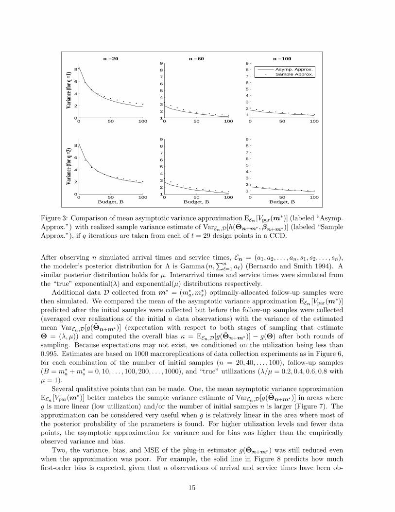
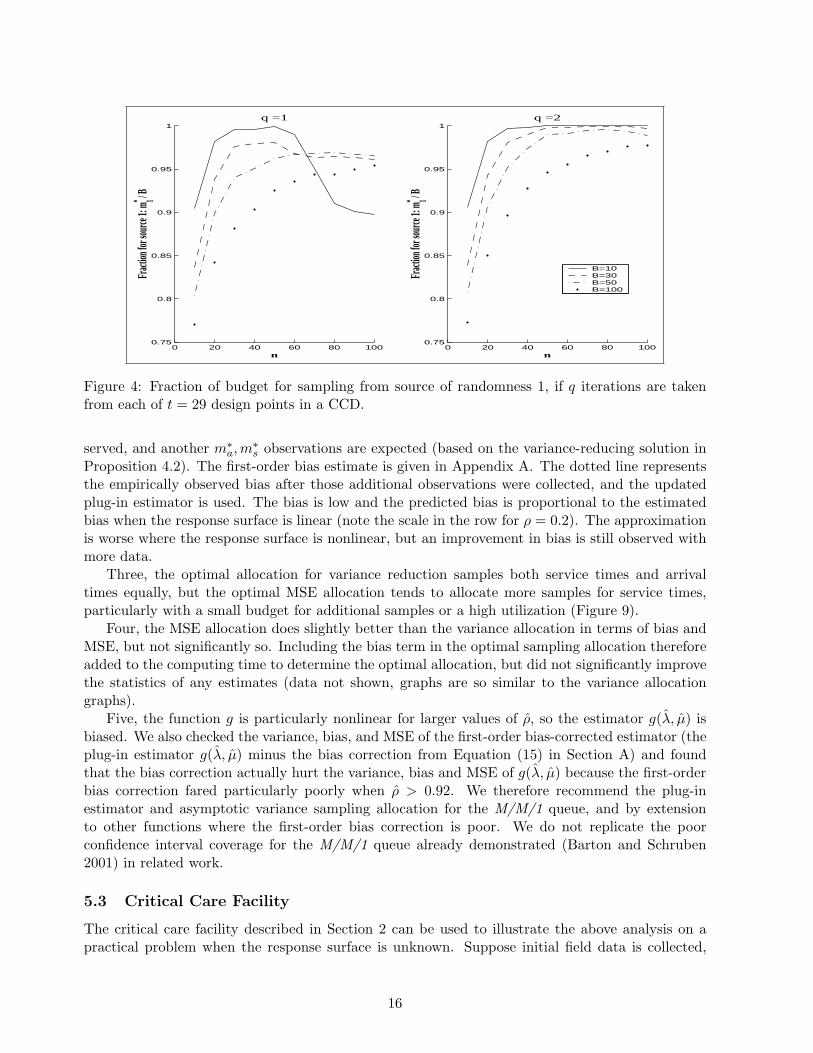
Figure 3 shows that EEn [Vpar(m∗)] and VarEn,D[h(Θn+m∗ , βn+m∗)] track each other reasonablywell, which is expected since the response is a low order polynomial. The allocations tended toallocate more samples from inputs with a larger variance and/or larger influence on the output(intuitive, so data not shown). In spite of the relatively close match of variance, Figure 4 indicatesthe fraction m∗

1/B of samples allocated to learning about the major quadratic term (µ1, λ1) variesas a function of B and n more significantly when there is less information about the responseparameters (small r = qt). This indicates that variability in the regression estimates may affectthe optimal data collection allocations.

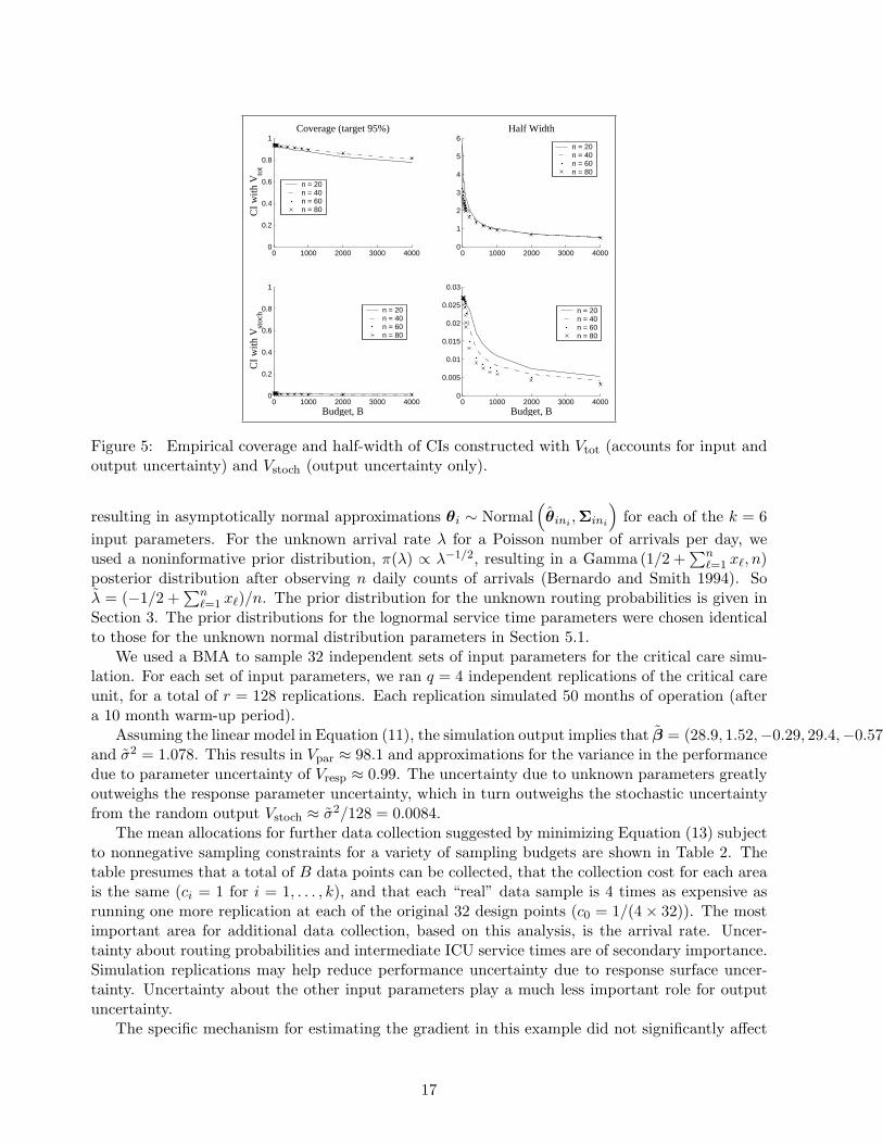
Figure 5 illustrates how significantly deleterious ignoring parameter uncertainty can be forthe coverage probability and the mean half-width size of confidence intervals. For this example,constructing 95% CI with stochastic uncertainty alone (using z97.5

√Vstoch) results in an extremely

poor coverage probability (about 0 to 2% rather than 95%) because input parameters are poorlyidentified. The wider CI half-widths based on z97.5

√Vtot result in much better coverage (empirical

coverage of 93-95%, very close to the nominal 95% level, when ni = n = 20, 40, 60, 80 data pointswere initially collected and when B = 0). For a fixed B, the coverage is worst when the leastamount of initial data is available (smaller n). For a fixed n, the coverage declined somewhat withincreasing B, dropping to 87-89% when B = 1000 and down further to 77-82% when B = 4000. For

13

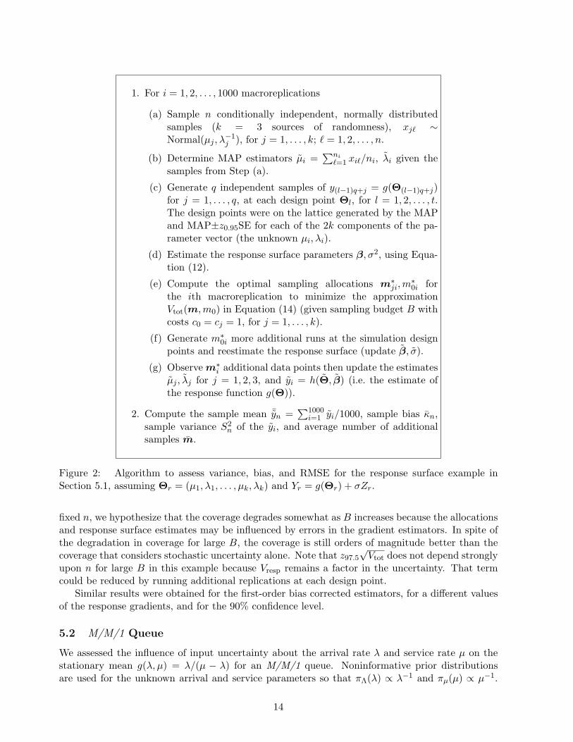
1. For i = 1, 2, . . . , 1000 macroreplications

(a) Sample n conditionally independent, normally distributedsamples (k = 3 sources of randomness), xj` ∼Normal(µj , λ

−1j ), for j = 1, . . . , k; ` = 1, 2, . . . , n.

(b) Determine MAP estimators µi =∑ni

`=1 xi`/ni, λi given thesamples from Step (a).

(c) Generate q independent samples of y(l−1)q+j = g(Θ(l−1)q+j)for j = 1, . . . , q, at each design point Θl, for l = 1, 2, . . . , t.The design points were on the lattice generated by the MAPand MAP±z0.95SE for each of the 2k components of the pa-rameter vector (the unknown µi, λi).

(d) Estimate the response surface parameters β, σ2, using Equa-tion (12).

(e) Compute the optimal sampling allocations m∗ji,m

∗0i for

the ith macroreplication to minimize the approximationVtot(m,m0) in Equation (14) (given sampling budget B withcosts c0 = cj = 1, for j = 1, . . . , k).

(f) Generate m∗0i more additional runs at the simulation design

points and reestimate the response surface (update β, σ).

(g) Observe m∗i additional data points then update the estimates

µj , λj for j = 1, 2, 3, and yi = h(Θ, β) (i.e. the estimate ofthe response function g(Θ)).

2. Compute the sample mean ¯yn =∑1000

i=1 yi/1000, sample bias κn,sample variance S2

n of the yi, and average number of additionalsamples m.

Figure 2: Algorithm to assess variance, bias, and RMSE for the response surface example inSection 5.1, assuming Θr = (µ1, λ1, . . . , µk, λk) and Yr = g(Θr) + σZr.

fixed n, we hypothesize that the coverage degrades somewhat as B increases because the allocationsand response surface estimates may be influenced by errors in the gradient estimators. In spite ofthe degradation in coverage for large B, the coverage is still orders of magnitude better than thecoverage that considers stochastic uncertainty alone. Note that z97.5

√Vtot does not depend strongly

upon n for large B in this example because Vresp remains a factor in the uncertainty. That termcould be reduced by running additional replications at each design point.

Similar results were obtained for the first-order bias corrected estimators, for a different valuesof the response gradients, and for the 90% confidence level.

5.2 M/M/1 Queue

We assessed the influence of input uncertainty about the arrival rate λ and service rate µ on thestationary mean g(λ, µ) = λ/(µ − λ) for an M/M/1 queue. Noninformative prior distributionsare used for the unknown arrival and service parameters so that πΛ(λ) ∝ λ−1 and πµ(µ) ∝ µ−1.

14

0 50 1000

2

4

6

8Va

rianc

e (fo

r q =1

)

n =20

0 50 1001

2

3

4

5

6

7

8

9n =60

0 50 100

1

2

3

4

5

6

7

8

9n =100

Asymp. Approx.Sample Approx.

0 50 1000

2

4

6

8

Varia

nce (

for q

=2)

Budget, B0 50 100

1

2

3

4

5

6

7

8

9

Budget, B0 50 100

1

2

3

4

5

6

7

8

9

Budget, B

Figure 3: Comparison of mean asymptotic variance approximation EEn [Vpar(m∗)] (labeled “Asymp.Approx.”) with realized sample variance estimate of VarEn,D[h(Θn+m∗ , βn+m∗)] (labeled “SampleApprox.”), if q iterations are taken from each of t = 29 design points in a CCD.

After observing n simulated arrival times and service times, En = (a1, a2, . . . , an, s1, s2, . . . , sn),the modeler’s posterior distribution for Λ is Gamma (n,

∑n`=1 a`) (Bernardo and Smith 1994). A

similar posterior distribution holds for µ. Interarrival times and service times were simulated fromthe “true” exponential(λ) and exponential(µ) distributions respectively.

Additional data D collected from m∗ = (m∗a, m

∗s) optimally-allocated follow-up samples were

then simulated. We compared the mean of the asymptotic variance approximation EEn [Vpar(m∗)]predicted after the initial samples were collected but before the follow-up samples were collected(averaged over realizations of the initial n data observations) with the variance of the estimatedmean VarEn,D[g(Θn+m∗)] (expectation with respect to both stages of sampling that estimateΘ = (λ, µ)) and computed the overall bias κ = EEn,D[g(Θn+m∗)] − g(Θ) after both rounds ofsampling. Because expectations may not exist, we conditioned on the utilization being less than0.995. Estimates are based on 1000 macroreplications of data collection experiments as in Figure 6,for each combination of the number of initial samples (n = 20, 40, . . . , 100), follow-up samples(B = m∗

a + m∗s = 0, 10, . . . , 100, 200, . . . , 1000), and “true” utilizations (λ/µ = 0.2, 0.4, 0.6, 0.8 with

µ = 1).Several qualitative points that can be made. One, the mean asymptotic variance approximation

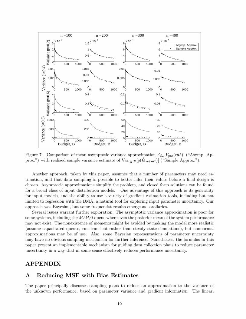
EEn [Vpar(m∗)] better matches the sample variance estimate of VarEn,D[g(Θn+m∗)] in areas whereg is more linear (low utilization) and/or the number of initial samples n is larger (Figure 7). Theapproximation can be considered very useful when g is relatively linear in the area where most ofthe posterior probability of the parameters is found. For higher utilization levels and fewer datapoints, the asymptotic approximation for variance and for bias was higher than the empiricallyobserved variance and bias.

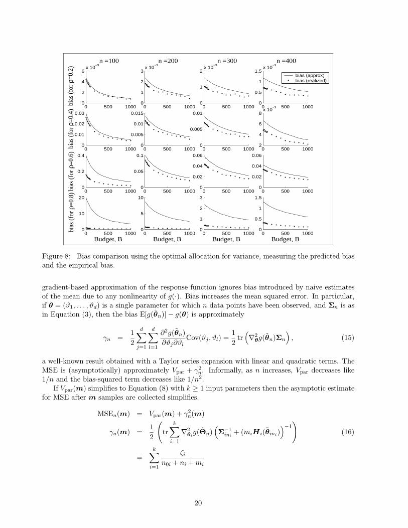
Two, the variance, bias, and MSE of the plug-in estimator g(Θn+m∗) was still reduced evenwhen the approximation was poor. For example, the solid line in Figure 8 predicts how muchfirst-order bias is expected, given that n observations of arrival and service times have been ob-

15

0 20 40 60 80 1000.75

0.8

0.85

0.9

0.95

1q =1

Fract

ion fo

r sou

rce 1:

m1* / B

n0 20 40 60 80 100

0.75

0.8

0.85

0.9

0.95

1q =2

Fract

ion fo

r sou

rce 1:

m1* / B

n

B=10B=30B=50B=100

Figure 4: Fraction of budget for sampling from source of randomness 1, if q iterations are takenfrom each of t = 29 design points in a CCD.

served, and another m∗a,m

∗s observations are expected (based on the variance-reducing solution in

Proposition 4.2). The first-order bias estimate is given in Appendix A. The dotted line representsthe empirically observed bias after those additional observations were collected, and the updatedplug-in estimator is used. The bias is low and the predicted bias is proportional to the estimatedbias when the response surface is linear (note the scale in the row for ρ = 0.2). The approximationis worse where the response surface is nonlinear, but an improvement in bias is still observed withmore data.

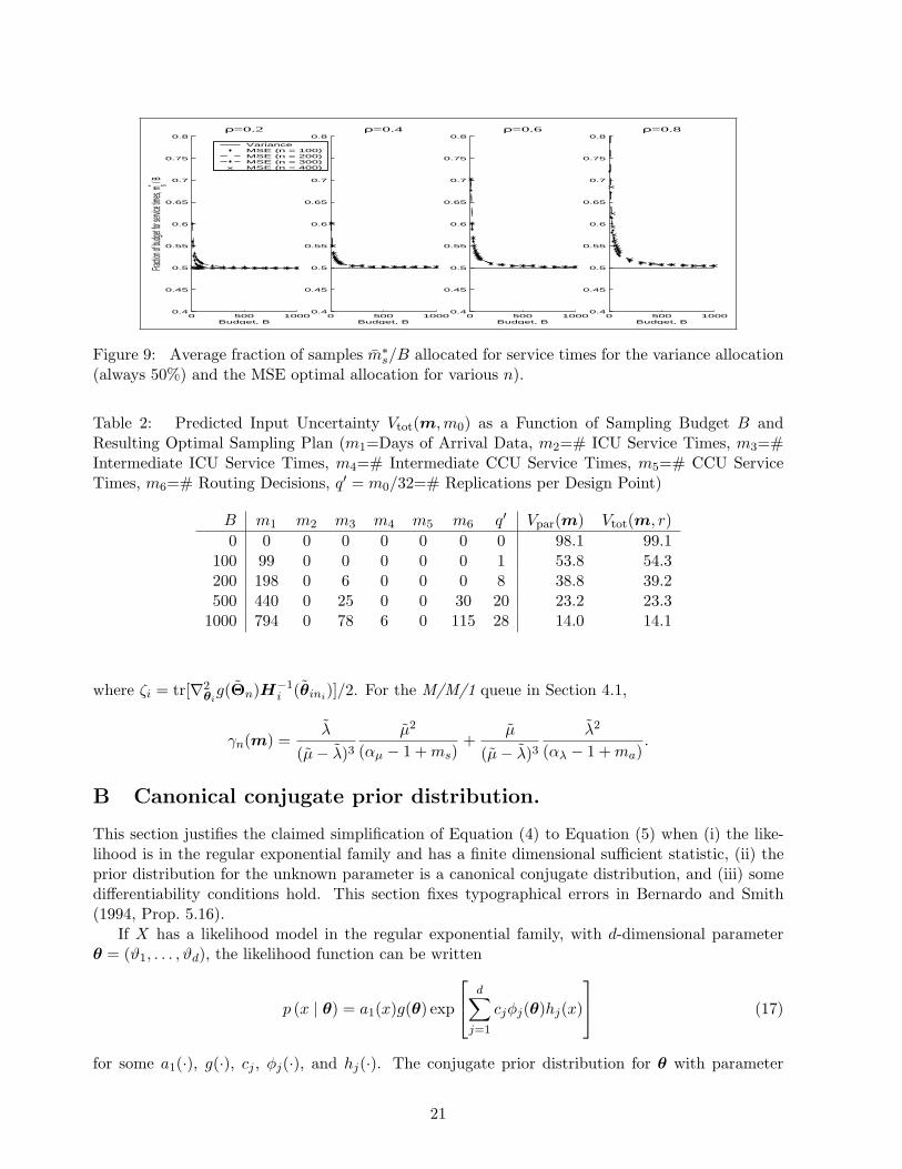
Three, the optimal allocation for variance reduction samples both service times and arrivaltimes equally, but the optimal MSE allocation tends to allocate more samples for service times,particularly with a small budget for additional samples or a high utilization (Figure 9).

Four, the MSE allocation does slightly better than the variance allocation in terms of bias andMSE, but not significantly so. Including the bias term in the optimal sampling allocation thereforeadded to the computing time to determine the optimal allocation, but did not significantly improvethe statistics of any estimates (data not shown, graphs are so similar to the variance allocationgraphs).

Five, the function g is particularly nonlinear for larger values of ρ, so the estimator g(λ, µ) isbiased. We also checked the variance, bias, and MSE of the first-order bias-corrected estimator (theplug-in estimator g(λ, µ) minus the bias correction from Equation (15) in Section A) and foundthat the bias correction actually hurt the variance, bias and MSE of g(λ, µ) because the first-orderbias correction fared particularly poorly when ρ > 0.92. We therefore recommend the plug-inestimator and asymptotic variance sampling allocation for the M/M/1 queue, and by extensionto other functions where the first-order bias correction is poor. We do not replicate the poorconfidence interval coverage for the M/M/1 queue already demonstrated (Barton and Schruben2001) in related work.

5.3 Critical Care Facility

The critical care facility described in Section 2 can be used to illustrate the above analysis on apractical problem when the response surface is unknown. Suppose initial field data is collected,

16

0 1000 2000 3000 40000

0.2

0.4

0.6

0.8

1Coverage (target 95%)

CI

with

Vto

t

n = 20n = 40n = 60n = 80

0 1000 2000 3000 40000

1

2

3

4

5

6Half Width

n = 20n = 40n = 60n = 80

0 1000 2000 3000 40000

0.2

0.4

0.6

0.8

1

CI

with

Vst

och

Budget, B

n = 20n = 40n = 60n = 80

0 1000 2000 3000 40000

0.005

0.01

0.015

0.02

0.025

0.03

Budget, B

n = 20n = 40n = 60n = 80

Figure 5: Empirical coverage and half-width of CIs constructed with Vtot (accounts for input andoutput uncertainty) and Vstoch (output uncertainty only).

resulting in asymptotically normal approximations θi ∼ Normal(θini ,Σini

)for each of the k = 6

input parameters. For the unknown arrival rate λ for a Poisson number of arrivals per day, weused a noninformative prior distribution, π(λ) ∝ λ−1/2, resulting in a Gamma (1/2 +

∑n`=1 x`, n)

posterior distribution after observing n daily counts of arrivals (Bernardo and Smith 1994). Soλ = (−1/2 +

∑n`=1 x`)/n. The prior distribution for the unknown routing probabilities is given in

Section 3. The prior distributions for the lognormal service time parameters were chosen identicalto those for the unknown normal distribution parameters in Section 5.1.

We used a BMA to sample 32 independent sets of input parameters for the critical care simu-lation. For each set of input parameters, we ran q = 4 independent replications of the critical careunit, for a total of r = 128 replications. Each replication simulated 50 months of operation (aftera 10 month warm-up period).

Assuming the linear model in Equation (11), the simulation output implies that β = (28.9, 1.52,−0.29, 29.4,−0.57, 11.5, 0.0018,−2.05, 0.045,−55.5,−9.64,−47.0),and σ2 = 1.078. This results in Vpar ≈ 98.1 and approximations for the variance in the performancedue to parameter uncertainty of Vresp ≈ 0.99. The uncertainty due to unknown parameters greatlyoutweighs the response parameter uncertainty, which in turn outweighs the stochastic uncertaintyfrom the random output Vstoch ≈ σ2/128 = 0.0084.

The mean allocations for further data collection suggested by minimizing Equation (13) subjectto nonnegative sampling constraints for a variety of sampling budgets are shown in Table 2. Thetable presumes that a total of B data points can be collected, that the collection cost for each areais the same (ci = 1 for i = 1, . . . , k), and that each “real” data sample is 4 times as expensive asrunning one more replication at each of the original 32 design points (c0 = 1/(4× 32)). The mostimportant area for additional data collection, based on this analysis, is the arrival rate. Uncer-tainty about routing probabilities and intermediate ICU service times are of secondary importance.Simulation replications may help reduce performance uncertainty due to response surface uncer-tainty. Uncertainty about the other input parameters play a much less important role for outputuncertainty.

The specific mechanism for estimating the gradient in this example did not significantly affect

17

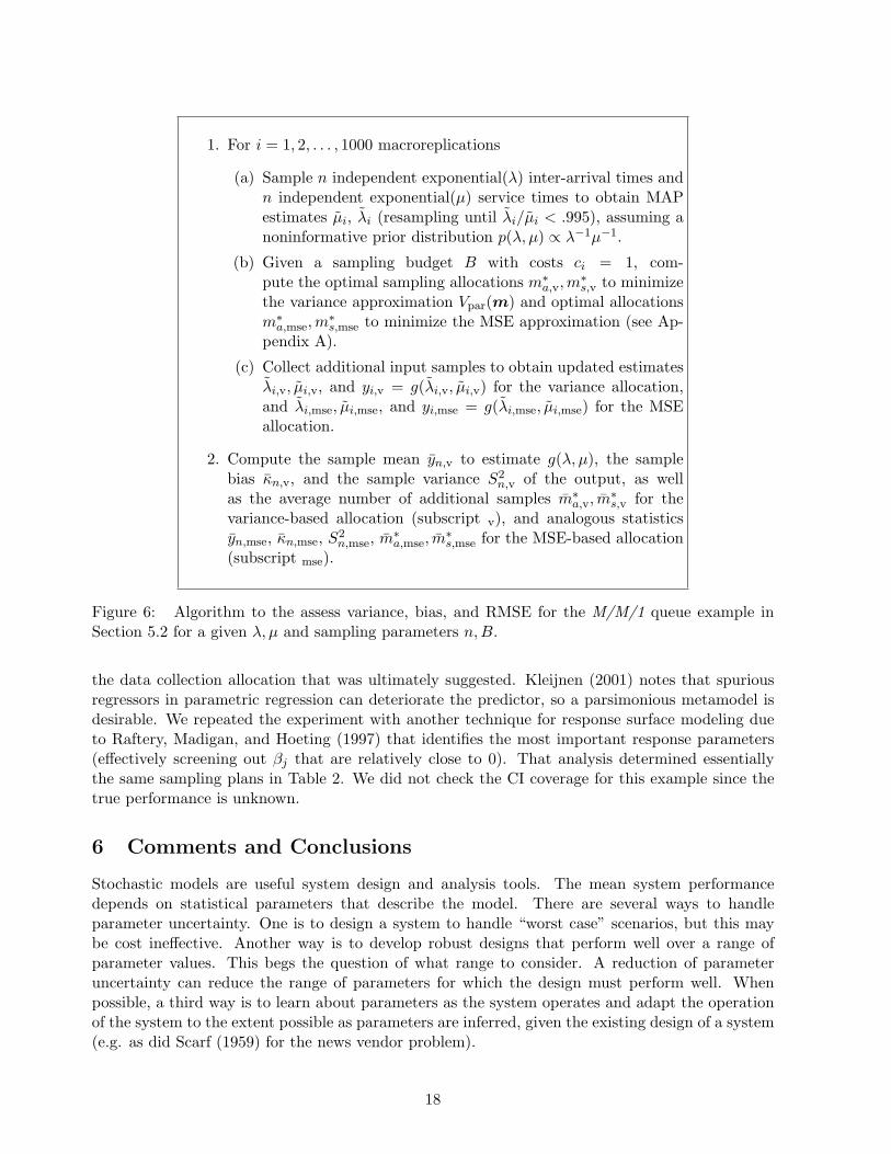
1. For i = 1, 2, . . . , 1000 macroreplications

(a) Sample n independent exponential(λ) inter-arrival times andn independent exponential(µ) service times to obtain MAPestimates µi, λi (resampling until λi/µi < .995), assuming anoninformative prior distribution p(λ, µ) ∝ λ−1µ−1.

(b) Given a sampling budget B with costs ci = 1, com-pute the optimal sampling allocations m∗

a,v,m∗s,v to minimize

the variance approximation Vpar(m) and optimal allocationsm∗

a,mse,m∗s,mse to minimize the MSE approximation (see Ap-

pendix A).

(c) Collect additional input samples to obtain updated estimatesλi,v, µi,v, and yi,v = g(λi,v, µi,v) for the variance allocation,and λi,mse, µi,mse, and yi,mse = g(λi,mse, µi,mse) for the MSEallocation.

2. Compute the sample mean yn,v to estimate g(λ, µ), the samplebias κn,v, and the sample variance S2

n,v of the output, as wellas the average number of additional samples m∗

a,v, m∗s,v for the

variance-based allocation (subscript v), and analogous statisticsyn,mse, κn,mse, S2

n,mse, m∗a,mse, m

∗s,mse for the MSE-based allocation

(subscript mse).

Figure 6: Algorithm to the assess variance, bias, and RMSE for the M/M/1 queue example inSection 5.2 for a given λ, µ and sampling parameters n,B.

the data collection allocation that was ultimately suggested. Kleijnen (2001) notes that spuriousregressors in parametric regression can deteriorate the predictor, so a parsimonious metamodel isdesirable. We repeated the experiment with another technique for response surface modeling dueto Raftery, Madigan, and Hoeting (1997) that identifies the most important response parameters(effectively screening out βj that are relatively close to 0). That analysis determined essentiallythe same sampling plans in Table 2. We did not check the CI coverage for this example since thetrue performance is unknown.

6 Comments and Conclusions

Stochastic models are useful system design and analysis tools. The mean system performancedepends on statistical parameters that describe the model. There are several ways to handleparameter uncertainty. One is to design a system to handle “worst case” scenarios, but this maybe cost ineffective. Another way is to develop robust designs that perform well over a range ofparameter values. This begs the question of what range to consider. A reduction of parameteruncertainty can reduce the range of parameters for which the design must perform well. Whenpossible, a third way is to learn about parameters as the system operates and adapt the operationof the system to the extent possible as parameters are inferred, given the existing design of a system(e.g. as did Scarf (1959) for the news vendor problem).

18

0 500 10000

1

2

3x 10

−3

Var

ianc

e (ρ

=0.2

)

n =100

0 500 10000

0.5

1

1.5x 10

−3

n =200

0 500 10002

4

6

8x 10

−4

n =300

0 500 10002

4

6

8x 10

−4

n =400

Asymp. Approx.Sample Approx.

0 500 10000

0.02

0.04

Var

ianc

e (ρ

=0.4

)

0 500 10000

0.005

0.01

0.015

0 500 10000

0.005

0.01

0 500 10000

0.005

0.01

0 500 10000

2

4

Var

ianc

e (ρ

=0.6

)

0 500 10000

0.2

0.4

0 500 10000

0.1

0.2

0 500 10000

0.05

0.1

0 500 10000

500

1000

Var

ianc

e (ρ

=0.8

)

Budget, B0 500 1000

0

200

400

Budget, B0 500 1000

0

20

40

60

Budget, B0 500 1000

0

10

20

30

Budget, B

Figure 7: Comparison of mean asymptotic variance approximation EEn [Vpar(m∗)] (“Asymp. Ap-prox.”) with realized sample variance estimate of VarEn,D[g(Θn+m∗)] (“Sample Approx.”).

Another approach, taken by this paper, assumes that a number of parameters may need es-timation, and that data sampling is possible to better infer their values before a final design ischosen. Asymptotic approximations simplify the problem, and closed form solutions can be foundfor a broad class of input distribution models. One advantage of this approach is its generalityfor input models, and the ability to use a variety of gradient estimation tools, including but notlimited to regression with the BMA, a natural tool for exploring input parameter uncertainty. Ourapproach was Bayesian, but some frequentist results emerge as corollaries.

Several issues warrant further exploration. The asymptotic variance approximation is poor forsome systems, including the M/M/1 queue where even the posterior mean of the system performancemay not exist. The nonexistence of moments might be avoided by making the model more realistic(assume capacitated queues, run transient rather than steady state simulations), but nonnormalapproximations may be of use. Also, some Bayesian representations of parameter uncertaintymay have no obvious sampling mechanism for further inference. Nonetheless, the formulas in thispaper present an implementable mechanism for guiding data collection plans to reduce parameteruncertainty in a way that in some sense effectively reduces performance uncertainty.

APPENDIX

A Reducing MSE with Bias Estimates

The paper principally discusses sampling plans to reduce an approximation to the variance ofthe unknown performance, based on parameter variance and gradient information. The linear,

19

0 500 10000

2

4

6x 10

−3

bias

(for

ρ=0

.2)

n =100

0 500 10000

1

2

3x 10

−3n =200

0 500 10000

1

2x 10

−3n =300

0 500 10000

0.5

1

1.5x 10

−3n =400

bias (approx)bias (realized)

0 500 10000

0.01

0.02

0.03

bias

(for

ρ=0

.4)

0 500 10000

0.005

0.01

0.015

0 500 10000

0.005

0.01

0 500 10002

4

6

8x 10

−3

0 500 10000

0.2

0.4

bias

(for

ρ=0

.6)

0 500 10000

0.05

0.1

0 500 10000

0.02

0.04

0.06

0 500 10000

0.02

0.04

0.06

0 500 10000

10

20

bias

(for

ρ=0

.8)

Budget, B0 500 1000

0

5

10

Budget, B0 500 1000

0

1

2

3

Budget, B0 500 1000

0

0.5

1

1.5

Budget, B

Figure 8: Bias comparison using the optimal allocation for variance, measuring the predicted biasand the empirical bias.

gradient-based approximation of the response function ignores bias introduced by naive estimatesof the mean due to any nonlinearity of g(·). Bias increases the mean squared error. In particular,if θ = (ϑ1, . . . , ϑd) is a single parameter for which n data points have been observed, and Σn is asin Equation (3), then the bias E[g(θn)]− g(θ) is approximately

γn =12

d∑

j=1

d∑

l=1

∂2g(θn)∂ϑj∂ϑl

Cov(ϑj , ϑl) =12

tr(∇2

θg(θn)Σn

), (15)

a well-known result obtained with a Taylor series expansion with linear and quadratic terms. TheMSE is (asymptotically) approximately Vpar + γ2

n. Informally, as n increases, Vpar decreases like1/n and the bias-squared term decreases like 1/n2.

If Vpar(m) simplifies to Equation (8) with k ≥ 1 input parameters then the asymptotic estimatefor MSE after m samples are collected simplifies.

MSEn(m) = Vpar(m) + γ2n(m)

γn(m) =12

(tr

k∑

i=1

∇2θi

g(Θn)(Σ−1

ini+ (miH i(θini)

)−1)

(16)

=k∑

i=1

ζi

n0i + ni + mi

20

0 500 10000.4

0.45

0.5

0.55

0.6

0.65

0.7

0.75

0.8ρ=0.2

Fractio

n of bu

dget fo

r servic

e times,

m s* / B

Budget, B0 500 1000

0.4

0.45

0.5

0.55

0.6

0.65

0.7

0.75

0.8ρ=0.4

Budget, B0 500 1000

0.4

0.45

0.5

0.55

0.6

0.65

0.7

0.75

0.8ρ=0.6

Budget, B0 500 1000

0.4

0.45

0.5

0.55

0.6

0.65

0.7

0.75

0.8ρ=0.8

Budget, B

VarianceMSE (n = 100)MSE (n = 200)MSE (n = 300)MSE (n = 400)

Figure 9: Average fraction of samples m∗s/B allocated for service times for the variance allocation

(always 50%) and the MSE optimal allocation for various n).

Table 2: Predicted Input Uncertainty Vtot(m,m0) as a Function of Sampling Budget B andResulting Optimal Sampling Plan (m1=Days of Arrival Data, m2=# ICU Service Times, m3=#Intermediate ICU Service Times, m4=# Intermediate CCU Service Times, m5=# CCU ServiceTimes, m6=# Routing Decisions, q′ = m0/32=# Replications per Design Point)

B m1 m2 m3 m4 m5 m6 q′ Vpar(m) Vtot(m, r)0 0 0 0 0 0 0 0 98.1 99.1

100 99 0 0 0 0 0 1 53.8 54.3200 198 0 6 0 0 0 8 38.8 39.2500 440 0 25 0 0 30 20 23.2 23.3

1000 794 0 78 6 0 115 28 14.0 14.1

where ζi = tr[∇2θi

g(Θn)H−1i (θini)]/2. For the M/M/1 queue in Section 4.1,

γn(m) =λ

(µ− λ)3µ2

(αµ − 1 + ms)+

µ

(µ− λ)3λ2

(αλ − 1 + ma).

B Canonical conjugate prior distribution.

This section justifies the claimed simplification of Equation (4) to Equation (5) when (i) the like-lihood is in the regular exponential family and has a finite dimensional sufficient statistic, (ii) theprior distribution for the unknown parameter is a canonical conjugate distribution, and (iii) somedifferentiability conditions hold. This section fixes typographical errors in Bernardo and Smith(1994, Prop. 5.16).

If X has a likelihood model in the regular exponential family, with d-dimensional parameterθ = (ϑ1, . . . , ϑd), the likelihood function can be written

p (x | θ) = a1(x)g(θ) exp

d∑

j=1

cjφj(θ)hj(x)

(17)

for some a1(·), g(·), cj , φj(·), and hj(·). The conjugate prior distribution for θ with parameter

21

n0, t = (t1, . . . , td) is

p (θ | n0, t) = [K(n0, t)]−1g(θ)n0 exp

d∑

j=1

cjφj(θ)tj

, (18)

where K(n0, t) =∫

g(θ)n0 exp[∑d

j=1 cjφj(θ)tj ]dθ < ∞.Suppose that the data x1, . . . , xn are observed. Set v`j = hj(x`) and v` = (v`1, . . . , v`d) with

sample average vn =∑n

`=1 v`/n. Then nvn is a sufficient statistic for θ and the posterior distri-bution of θ is p (θ | n0 + n, t + nvn).

A final reparametrization is useful. Set ψj = cjφj(θ) and ψ = (ψ1, . . . , ψd). Equation (17)can be rewritten in what is known as canonical conjugate form (Bernardo and Smith 1994, Defini-tion 4.12),

p (v` | ψ) = a2(v) exp[v`ψ

T − b(ψ)]

for some real-valued a2(v), b(ψ). The canonical conjugate prior distribution is

p (ψ | n0, t) = c(n0, t) exp[n0tψ

T − n0b(ψ)],

where n0, t = (t1, . . . , td) are parameters of the prior distribution.Bernardo and Smith (1994, Prop. 5.16) note that the posterior distribution has the same func-

tional form as the prior distribution,

p (ψ | n0, t,v1, v2, . . . , vn) = p (ψ | n0 + n, n0t + nvn).

Further, if ψ is the MAP estimator of ψ, then(Σ−1

n

)jl

= (n0 +n) ∂2b(ψ)∂ψj∂ψl

∣∣ψ=ψ

. The claim is provenby noting that the expected information in one observation is

(H(ψ))jl = E[

∂2b(ψ)∂ψj∂ψl

] ∣∣∣∣ψ

=∂2b(ψ)∂ψj∂ψl

∣∣∣∣ψ

.

The relationship also holds in the θ coordinate system if the map from ψ to θ is bijective in aneighborhood of ψ.

C Proof of Proposition 4.2.

Using the method of Lagrange multipliers, we obtain the Lagrangian function

L(m, τ) = Vpar(m)−k∑

i=1

τ (cimi −B)

=k∑

i=1

ξi

n0i + ni + mi−

k∑

i=1

τ (cimi −B) ,

where τ is the Lagrange multiplier. Set the (k + 1) partial derivatives to 0 to get

− ξi

(n0i + ni + mi)2− τci = 0, for i = 1, . . . , k, and (19)

k∑

i=1

cimi −B = 0. (20)

22

Equation (19) implies ξi/ci

(n0i+ni+mi)2= ξj/cj

(n0j+nj+mj)2. After some algebra we get

cj(n0j + nj + mj) =(

ξjcicj

ξi

)1/2

(n0i + ni + mi). (21)

Equation (20) can be rewritten∑k

j=1 cj(n0j + nj + mj) = B +∑k

`=1 c`(n0` + n`). SubstituteEquation (21) into this expression to obtain

(n0i + ni + mi)k∑

j=1

(ξjcicj

ξi

)1/2

= B +k∑

`=1

c`(n0` + n`). (22)

Algebraic rearranging gives the claimed result for the optimal m∗i ,

m∗i =

B +∑k

`=1 c`(n0` + n`)∑k

j=1

(ξjcicj

ξi

)1/2− (n0i + ni).

When B is sufficiently large, the constraint m∗i ≥ 0 is satisfied as desired.

Acknowledgments: We thank Jim Wilson for thorough and helpful feedback.

Bibliography

Barton, R. R. and L. W. Schruben (2001). Simulating real systems. in submission.

Bernardo, J. M. and A. F. M. Smith (1994). Bayesian Theory. Chichester, UK: Wiley.

Box, G. and N. Draper (1987). Empirical Model-Building and Response Surfaces. New York:Wiley.

Box, G., W. Hunter, and J. Hunter (1978). Statistics for Experimenters. An Introduction toDesign, Data Analysis and Model Building. New York: Wiley.

Buzacott, J. A. and J. G. Shanthikumar (1993). Stochastic Models of Manufacturing Systems.Englewood Cliffs, New Jersey: Prentice-Hall, Inc.

Cheng, R. C. H. and W. Holland (1997). Sensitivity of computer simulation experiments to errorsin input data. J. Statistical Computing and Simulation 57, 219–241.

Cheng, R. C. H. and W. Holland (2004). Calculation of confidence intervals for simulation output.ACM Transactions on Modeling and Computer Simulation 14 (4), 344–362.

Chick, S. E. (1997). Bayesian analysis for simulation input and output. In S. Andradottir,K. Healy, D. Withers, and B. Nelson (Eds.), Proc. 1997 Winter Simulation Conference,Piscataway, NJ, pp. 253–260. IEEE, Inc.

Chick, S. E. (2001). Input distribution selection for simulation experiments: Accounting for inputuncertainty. Operations Research 49 (5), 744–758.

Draper, D. (1995). Assessment and propogation of model uncertainty (with discussion). J. RoyalStatistical Society, Series B 57 (1), 45–97.

Edwards, A. W. F. (1984). Likelihood. Cambridge University Press.

Gelman, A., J. B. Carlin, H. S. Stern, and D. R. Rubin (1995). Bayesian Data Analysis. London:Chapman & Hall.

23

Kleijnen, J. P. C. (2001). Comments on M.C. Kennedy & A. O’Hagan’s ‘Bayesian calibration ofcomputer models’. Journal Royal Statistical Society, Series B 63 (3), in press.

Law, A. M. and W. D. Kelton (2000). Simulation Modeling & Analysis (3rd ed.). New York:McGraw-Hill, Inc.

Mendoza, M. (1994). Asymptotic normality under transformations. A result with Bayesian ap-plications. TEST 3 (2), 173–180.

Myers, R., A. Khuri, and W. Carter (1989). Response surface methodology: 1966-1988. Techno-metrics 31 (2), 137–157.

Ng, S.-H. and S. E. Chick (2001). Reducing input distribution uncertainty for simulations. InB. Peters, J. Smith, M. Rohrer, and D. Madeiros (Eds.), Proc. 2001 Winter SimulationConference, Piscataway, NJ, pp. 364–371. IEEE, Inc.

Raftery, A. E., D. Madigan, and J. A. Hoeting (1997). Bayesian model averaging for linearregression models. Journal of the American Statistical Association 92 (437), 179–191.

Scarf, H. (1959). Bayes solutions of the statistical inventory problem. Annals of MathematicalStatistics 30, 490–508.

Schervish, M. J. (1995). Theory of Statistics. New York: Springer.

Schruben, L. W. and B. H. Margolin (1978). Pseudorandom number assignment in statisticallydesigned simulation and distribution sampling experiments. Journal of the American Statis-tical Association 73 (363), 504–525.

Serfling, R. J. (1980). Approximation Theorems of Mathematical Statistics. New York: Wiley.

Zouaoui, F. and J. R. Wilson (2001). Accounting for input model and parameter uncertainty insimulation input modeling. In B. Peters, J. Smith, M. Rohrer, and D. Madeiros (Eds.), Proc.2001 Winter Simulation Conference, Piscataway, NJ, pp. 290–299. IEEE, Inc.

Zouaoui, F. and J. R. Wilson (2003). Accounting for parameter uncertainty in simulation inputmodeling. IIE Transactions 35, 781–792.

Zouaoui, F. and J. R. Wilson (2004). Accounting for input-model and input-parameter uncer-tainties in simulation. IIE Transactions 36 (11), 1135–1151.

24