


Languages
Pages
Legal


RADIO OCCULTATION OF SATURN’S RINGS WITH THE
CASSINI SPACECRAFT: RING MICROSTRUCTURE INFERRED
FROM NEAR-FORWARD RADIO WAVE SCATTERING
A DISSERTATION
SUBMITTED TO THE DEPARTMENT OF ELECTRICAL
ENGINEERING
AND THE COMMITTEE ON GRADUATE STUDIES
OF STANFORD UNIVERSITY
IN PARTIAL FULFILLMENT OF THE REQUIREMENTS
FOR THE DEGREE OF
DOCTOR OF PHILOSOPHY
Fraser Stuart Thomson
July 2010

http://creativecommons.org/licenses/by-nc/3.0/us/
This dissertation is online at: http://purl.stanford.edu/pb657pg3502
© 2010 by Fraser Stuart Thomson. All Rights Reserved.
Re-distributed by Stanford University under license with the author.
This work is licensed under a Creative Commons Attribution-Noncommercial 3.0 United States License.
ii
I certify that I have read this dissertation and that, in my opinion, it is fully adequatein scope and quality as a dissertation for the degree of Doctor of Philosophy.
Howard Zebker, Primary Adviser
I certify that I have read this dissertation and that, in my opinion, it is fully adequatein scope and quality as a dissertation for the degree of Doctor of Philosophy.
Per Enge
I certify that I have read this dissertation and that, in my opinion, it is fully adequatein scope and quality as a dissertation for the degree of Doctor of Philosophy.
Essam Marouf
Approved for the Stanford University Committee on Graduate Studies.
Patricia J. Gumport, Vice Provost Graduate Education
This signature page was generated electronically upon submission of this dissertation in electronic format. An original signed hard copy of the signature page is on file inUniversity Archives.
iii

iv

Abstract
The Cassini spacecraft is a robotic probe sent from Earth to orbit and explore the
planet Saturn, its moons, and its expansive ring system. Between May 3 and Au-
gust 2 of 2005, we undertook a series of radio occultation experiments, during which
the Cassini spacecraft operated in conjunction with the NASA Deep Space Network
(DSN) to probe the rings at three distinct radio wavelengths.
During our occultation experiments, Cassini flies behind the rings of Saturn as
viewed from Earth and transmits coherent radio signals at wavelengths of 13 cm, 3.6
cm, and 0.94 cm, in the radio bands known as S, X, and Ka, respectively. These
signals pass through the rings and are received and recorded on Earth at the large
antenna complexes of the DSN. At each of the three transmitted frequency channels,
the received signal comprises two components, i) a direct (coherent) component, which
is the transmitted sinusoid, attenuated and phase shifted by the average effect of its
interaction with the interceding ring material, and ii) a scattered (incoherent) signal
component, comprising energy that is forward-scattered towards the receiver from all
of the ring particles illuminated by the transmitting antenna’s beam. The time- and
spatially-averaged diffraction signature of ring microstructure—which forms when
individual ring particles organize into large clusters or groups under the influence of
collisional and self-gravitational forces—is superimposed on the scattered signal.
Coherent radio waves transmitted by the Cassini spacecraft are diffracted at vari-
ous locations in Ring A and B and indicate the presence of fine-scale structure showing
periodic variation in optical depth, which we refer to as periodic microstructure (PM).
We interpret the observed spectral signature using simple diffraction grating models,
yielding estimates of the structural period λgr ≈ 100–250 meters. In particular, two
v

regions in Ring A at radial locations 123.05–123.4 × 10³ km and 123.6–124.6 × 10³
km yield average estimates of λgr=163+−6 meters and λgr=217+−8 meters, respectively.
Three regions in Ring B at radial locations 92.1–92.6 × 10³ km, 99.0–104.5 × 10³
km, and 110.0–115.0 × 10³ km yield average estimates of λgr=115+20−15, 146
+−14, and
250+150−75 meters, respectively. In all regions, the structure appears to be azimuthally
symmetric with mean orientation angles ranging between -2.8o ≤ φgr ≤ 1.5o.
Prior to Cassini, axisymmetric periodic microstructure was predicted by fluid
dynamical theory and by the results of dynamical simulations of the rings, but was
not observed experimentally. Our observations are the first to directly observe PM
in the rings, and to report estimates of its structural period and orientation in five
distinct regions across Rings A and B.
vi

Acknowledgements
I would like to extend my heartfelt thanks to Howard Zebker for taking over from
Len Tyler as my primary advisor in early 2008. Without his support, it is unlikely
that I would have completed this degree program. I will always be in his debt for his
acts of kindness and support.
Sincere thanks are due to Essam Marouf, who always made the effort to find time
in his busy schedule for my many questions. Essam has been a model of patience,
diligence, and excellence during our years of collaboration, and his steady provision of
guidance, tutelage, and financial support has made this work possible. His ethics and
commitment to excellence in his work form an ideal that all scientists should aspire
to, and which many on the Cassini radio science team depend on and are indebted
to. One of the most memorable moments in my life is being at JPL during the first
planned Cassini radio occultation experiment, and watching how excited Essam and
Dick French were as we all watched the spectrum of the received signal varying in
real time, as the experiment revealed hints of ring structure. Throughout my years
at Stanford, it has been a great privilege and joy for me to observe Essam’s passion
for the rings firsthand.
Thanks also to Per Enge for serving as my third reader, for serving on my oral
defense committee, and for teaching me about orbital mechanics and GPS. He is an
excellent professor and a friend to many students, myself included.
I extend many thanks to my teacher and friend Ivan Linscott, who always has
time to discuss new ideas and old ones, and for being such a generous friend to many
students over the years. Thanks also to Antony Fraser-Smith for stepping in to save
the day on several occasions, for serving on my defense committee, and for being such
vii
a great guy in general.
Special thanks go to Len Tyler for all of his time, energy, and support, and for
being a mentor to me for several years prior to his semi-retirement. Len is a polymath,
and memories of times when I have glimpsed his brilliance will always bring a smile
to my face. On those rare occasions when Len did not know the answer, his honest
and free willingness to admit gaps in his knowledge provide an inspirational lesson to
us all; there is no better way to get started solving a problem than to admit what is
known and what is not known. Len’s insistent attention to detail has taught me to
choose my words more carefully, and has made me a better technical writer. As Len
would say, a key goal in writing is to minimize the impedance mismatch between the
writer and their audience. I hope I have done that here.
A very special thanks to Sami Asmar of NASA’s Jet Propulsion Laboratory, for
being a friend and a great boss during my all-too-brief work terms at the lab. I would
be honored to work with him or for him again, anytime and anywhere. I would also
like to thank Christopher Chyba, my friend and mentor, and one of the kindest and
smartest people I’ve ever known. The nine months that we collaborated before I
chose to join Cassini was the most exciting and fulfilling period of time that I spent
at Stanford.
Lots of love and thanks to my parents, who provided access to all of the oppor-
tunities that anyone could ever ask for in life. I would not be writing this without
them. There are many other people who, either knowingly or unknowingly, helped to
make this dissertation possible. To the anonymous, I offer my thanks also.
I dedicate this dissertation to my wife Katherine and to my son Kaiden (b. June
7, 2009), for showing me how simple life really is, and for being a constant reminder
of what is truly important.
This work was supported by the NASA Cassini Project through JPL Contract
No. 1214216. The support is gratefully acknowledged.
viii
Contents
Abstract v
Acknowledgements vii
1 Introduction and Historical Review 11
1.1 The Discovery of Saturn’s Rings . . . . . . . . . . . . . . . . . . . . . 12
1.2 Occultation Studies of Saturn’s Rings: A Brief History . . . . . . . . 20
1.3 Contents and Contributions of this Dissertation . . . . . . . . . . . . 22
2 Saturn Ring Structure and Dynamics 27
2.1 Ring Macrostructure . . . . . . . . . . . . . . . . . . . . . . . . . . . 33
2.1.1 Gaps and Ring Boundaries . . . . . . . . . . . . . . . . . . . . 34
2.1.2 Spiral Density and Bending Waves . . . . . . . . . . . . . . . 38
2.2 Ring Microstructure . . . . . . . . . . . . . . . . . . . . . . . . . . . 40
2.2.1 Gravitational Wakes . . . . . . . . . . . . . . . . . . . . . . . 40
2.2.2 Periodic Microstructure . . . . . . . . . . . . . . . . . . . . . 42
2.3 Models of Ring Microstructure . . . . . . . . . . . . . . . . . . . . . . 44
2.4 Summary . . . . . . . . . . . . . . . . . . . . . . . . . . . . . . . . . 47
3 EM Scattering and Diffraction from Ring Particle Clusters 49
3.1 Introduction . . . . . . . . . . . . . . . . . . . . . . . . . . . . . . . . 50
3.2 Theoretical Background . . . . . . . . . . . . . . . . . . . . . . . . . 53
3.2.1 Coherent Scattering from a Sphere: Mie Theory . . . . . . . . 56
3.2.2 Multi-Particle Scattering Using Mie Theory . . . . . . . . . . 60
ix

3.2.3 Diffraction from an Amplitude Screen . . . . . . . . . . . . . . 64
3.2.4 Mie and Diffraction Theory: Some Practical Considerations . 66
3.3 Simulation Results . . . . . . . . . . . . . . . . . . . . . . . . . . . . 68
3.3.1 Scattering from a Single Sphere . . . . . . . . . . . . . . . . . 70
3.3.2 Scattering from Two and Three Spheres . . . . . . . . . . . . 71
3.3.3 Scattering from Ten Spheres . . . . . . . . . . . . . . . . . . . 77
3.4 Discussion . . . . . . . . . . . . . . . . . . . . . . . . . . . . . . . . . 83
3.5 Amplitude Screen Model Results for Thick, Homogeneous Rings . . . 86
3.5.1 An Analytic Solution for Forward Scattering . . . . . . . . . . 87
3.5.2 Comparison with the Amplitude Screen Model . . . . . . . . . 89
3.6 Summary . . . . . . . . . . . . . . . . . . . . . . . . . . . . . . . . . 95
4 The Cassini Radio Occultation Experiment 97
4.1 Techniques, Observables, and Properties of the Received Signal . . . . 98
4.1.1 Transmitted and Received Signals . . . . . . . . . . . . . . . . 98
4.1.2 Trajectory Design and Doppler Contours . . . . . . . . . . . . 101
4.1.3 Observables . . . . . . . . . . . . . . . . . . . . . . . . . . . . 105
4.2 Detection of Microstructure in the Rings . . . . . . . . . . . . . . . . 111
4.2.1 Diffraction from Ring Microstructure . . . . . . . . . . . . . . 111
4.2.2 Evidence of Ring Microstructure . . . . . . . . . . . . . . . . . 113
4.3 Cassini Ring Occultation Observations, May–August 2005 . . . . . . 119
4.3.1 Details of the REV 7–12 Observations . . . . . . . . . . . . . 120
4.4 Summary . . . . . . . . . . . . . . . . . . . . . . . . . . . . . . . . . 130
5 Fitting Microstructure Models to Radio Occultation Data 131
5.1 Overview of the Method . . . . . . . . . . . . . . . . . . . . . . . . . 131
5.2 Microstructure Modeling Techniques . . . . . . . . . . . . . . . . . . 134
5.2.1 Microstructure Simulations using the Amplitude Screen Method 134
5.2.2 Microstructure Modeling using Analytic Methods . . . . . . . 142
5.3 Comparing Model Behavior with Radio Occultation Measurements . . 146
5.3.1 General Approach . . . . . . . . . . . . . . . . . . . . . . . . . 147
5.3.2 Periodic Microstructure . . . . . . . . . . . . . . . . . . . . . 157
x

5.4 Least-Squares Fitting of Model Parameters to the Data . . . . . . . . 158
5.4.1 Fitting Models of Periodic Microstructure . . . . . . . . . . . 159
5.4.2 Other Models . . . . . . . . . . . . . . . . . . . . . . . . . . . 163
5.5 Summary . . . . . . . . . . . . . . . . . . . . . . . . . . . . . . . . . 163
6 Periodic Microstructure in Saturn’s Rings 165
6.1 A Survey of Periodic Microstructure in Saturn’s Rings . . . . . . . . 166
6.2 Estimates of Physical Parameters λgr and φgr . . . . . . . . . . . . . . 173
6.3 Optical Depth Variation within Features A123.2 and A124.1 . . . . . 184
6.4 Discussion . . . . . . . . . . . . . . . . . . . . . . . . . . . . . . . . . 184
6.4.1 Concurrent Microstructure . . . . . . . . . . . . . . . . . . . . 184
6.4.2 The Onset of Viscous Overstability . . . . . . . . . . . . . . . 185
6.4.3 Optical Depth Characteristics of PM Regions . . . . . . . . . 188
6.5 Summary . . . . . . . . . . . . . . . . . . . . . . . . . . . . . . . . . 192
7 Summary and Conclusions 195
7.1 General Results . . . . . . . . . . . . . . . . . . . . . . . . . . . . . . 195
7.2 Assumptions and Limitations . . . . . . . . . . . . . . . . . . . . . . 196
7.3 Contributions . . . . . . . . . . . . . . . . . . . . . . . . . . . . . . . 198
7.4 Future Work . . . . . . . . . . . . . . . . . . . . . . . . . . . . . . . . 198
A Radio Occultation Studies of Planetary Rings 201
A.1 Optical Depth Profiles . . . . . . . . . . . . . . . . . . . . . . . . . . 201
A.1.1 Circular Rings . . . . . . . . . . . . . . . . . . . . . . . . . . . 203
A.1.2 Elliptical Rings . . . . . . . . . . . . . . . . . . . . . . . . . . 205
A.1.3 Resolution Limitations in the Reconstruction Process . . . . . 206
A.1.4 Profiling Ring Optical Depth . . . . . . . . . . . . . . . . . . 209
A.2 Particle Size Distributions . . . . . . . . . . . . . . . . . . . . . . . . 211
A.2.1 Suprameter-Sized Particles . . . . . . . . . . . . . . . . . . . . 212
A.2.2 Submeter-Sized Particles . . . . . . . . . . . . . . . . . . . . . 215
A.2.3 Surface Mass Density and Ring Thickness . . . . . . . . . . . 216
A.3 Summary . . . . . . . . . . . . . . . . . . . . . . . . . . . . . . . . . 217
xi

B Cassini 2005 Radio Occultation Timelines 219
C Historically Important Articles on Saturn’s Rings 231
C.1 Christiaan Huygens’ article on Saturn’s Ring . . . . . . . . . . . . . . 231
C.2 Cassini’s Paper on his Eponymous Division . . . . . . . . . . . . . . . 237
D Limitations on the Use of the Power-Law form of Sy(f) to Compute
Allan Variance 241
D.1 Abstract . . . . . . . . . . . . . . . . . . . . . . . . . . . . . . . . . . 241
D.2 Introduction . . . . . . . . . . . . . . . . . . . . . . . . . . . . . . . . 242
D.3 Exact and Approximate Solutions for σ2y(τ) . . . . . . . . . . . . . . . 243
D.3.1 Evaluation of the f−2-term . . . . . . . . . . . . . . . . . . . . 243
D.3.2 Evaluation of the f−1-term . . . . . . . . . . . . . . . . . . . . 244
D.3.3 Evaluation of the f 0-term . . . . . . . . . . . . . . . . . . . . 245
D.3.4 Evaluation of the f 1-term . . . . . . . . . . . . . . . . . . . . 246
D.3.5 Evaluation of the f 2-term . . . . . . . . . . . . . . . . . . . . 247
D.4 Results and Conclusions . . . . . . . . . . . . . . . . . . . . . . . . . 247
E Radon and Abel Transform Equivalence in Atmospheric Radio Oc-
cultation 253
E.1 Abstract . . . . . . . . . . . . . . . . . . . . . . . . . . . . . . . . . . 253
E.2 Introduction . . . . . . . . . . . . . . . . . . . . . . . . . . . . . . . . 254
E.3 Atmospheric Radio Occultation . . . . . . . . . . . . . . . . . . . . . 254
E.4 Applicability of the Abel Transform in Radio Occultation . . . . . . . 256
E.5 The Radon Transform . . . . . . . . . . . . . . . . . . . . . . . . . . 257
E.6 Radon and Abel Transform Equivalence for Radio Occultation . . . . 258
E.7 Discussion and Conclusion . . . . . . . . . . . . . . . . . . . . . . . . 260
E.8 Derivation of Eq. (E.4) . . . . . . . . . . . . . . . . . . . . . . . . . . 261
xii
List of Tables
1.1 Key Milestones in the Study of Saturn’s Rings . . . . . . . . . . . . . 18
2.1 Properties of Saturn’s Ring System . . . . . . . . . . . . . . . . . . . 32
3.1 Summary of Two-Sphere Scattering Investigations (x = 40) . . . . . . 76
3.2 Summary of Three-Sphere Scattering Investigations (x = 40) . . . . . 77
3.3 Summary of Ten-Sphere Scattering Investigations (Monodistribution,
x = 40) . . . . . . . . . . . . . . . . . . . . . . . . . . . . . . . . . . 79
3.4 Summary of Ten-Sphere Scattering Investigations (Uniform Distribu-
tion, 40 ≤ x ≤ 80) . . . . . . . . . . . . . . . . . . . . . . . . . . . . . 83
4.1 Summary of Geometric Occultation Parameters . . . . . . . . . . . . 125
6.1 Summary of PM Features in the Rings . . . . . . . . . . . . . . . . . 175
D.1 One Percent Convergence Conditions for the Exact Solution and the
Approximate Solution to Each Term in the Power-Law Formulation of
Allan Variance . . . . . . . . . . . . . . . . . . . . . . . . . . . . . . 249
xiii

List of Figures
1.1 Sketch of Saturn as seen by Galileo in 1610 . . . . . . . . . . . . . . . 12
1.2 Sketch of Saturn as seen by Galileo in 1616 . . . . . . . . . . . . . . . 13
1.3 Early Drawings of Saturn published by Christiaan Huygens in Systema
Saturnium (1659) . . . . . . . . . . . . . . . . . . . . . . . . . . . . . 14
1.4 Huygens’ Thick Disc Conceptualization of Saturn’s Rings . . . . . . . 15
1.5 Cassini’s Sketch of Cassini Division (1676) . . . . . . . . . . . . . . . 16
1.6 Diagram of the Rings and Moons of the Giant Planets . . . . . . . . 19
2.1 Structure of Saturn’s Rings . . . . . . . . . . . . . . . . . . . . . . . 29
2.2 Saturn’s Main Rings and Ring F . . . . . . . . . . . . . . . . . . . . . 30
2.3 Particle Size Distributions in Saturn’s Cassini Division and Ring A . 31
2.4 Keeler Gap with Daphnis . . . . . . . . . . . . . . . . . . . . . . . . . 35
2.5 Gaps, Density and Bending Waves in Ring A . . . . . . . . . . . . . . 36
2.6 Propeller Features in Saturn’s Rings . . . . . . . . . . . . . . . . . . 37
2.7 Density and Bending Waves . . . . . . . . . . . . . . . . . . . . . . . 39
2.8 Gravitational Wakes . . . . . . . . . . . . . . . . . . . . . . . . . . . 41
2.9 Periodic Microstructure . . . . . . . . . . . . . . . . . . . . . . . . . . 43
2.10 Artist’s Rendition of Fine-Scale Ring Structure . . . . . . . . . . . . 43
2.11 A Survey of Ring Microstructure . . . . . . . . . . . . . . . . . . . . 45
2.12 Models of Ring Microstructure . . . . . . . . . . . . . . . . . . . . . . 46
3.1 Construction of the Diffraction Screen . . . . . . . . . . . . . . . . . 54
3.2 Comparison of Mie Theory and Diffraction Theory: Single Sphere . . 72
3.3 Geometry Definition for Two and Three Sphere Scattering Models . . 73
xiv

3.4 Comparison of Mie Theory and Diffraction Theory: Two Spheres . . 75
3.5 Comparison of Mie Theory and Diffraction Theory: Three Spheres . . 78
3.6 Comparison of Mie Theory and Diffraction Theory: Ten Identical Spheres 80
3.7 Comparison of Mie Theoretic Solutions for Lossy vs. Lossless Spheres 81
3.8 Comparison of Mie Theory and Diffraction Theory: Ten Spheres Sam-
pled from a Uniform Size Distribution . . . . . . . . . . . . . . . . . . 82
3.9 Ten Spheres and their Diffraction Pattern . . . . . . . . . . . . . . . 84
3.10 Amplitude Screen Models of Homogeneous, MPT Rings . . . . . . . . 90
3.11 Comparison of the Amplitude Screen Method with the Theory ofMarouf
et al. [1982] . . . . . . . . . . . . . . . . . . . . . . . . . . . . . . . . 92
4.1 Ring Occultation Geometry . . . . . . . . . . . . . . . . . . . . . . . 99
4.2 Occultation Geometry and Doppler Contours . . . . . . . . . . . . . . 102
4.3 Ring Occultation Signal Properties . . . . . . . . . . . . . . . . . . . 107
4.4 Doppler Signature of a Gap in the Rings . . . . . . . . . . . . . . . . 109
4.5 Diffraction from Microstructure in Saturn’s Rings . . . . . . . . . . . 115
4.6 Doppler Signature of Periodic Microstructure in the Rings . . . . . . 117
4.7 DSN Complex Locations . . . . . . . . . . . . . . . . . . . . . . . . . 119
4.8 Ring Longitude of Occultation Tracks, May–August 2005 . . . . . . . 121
4.9 Distance from Cassini to the Ring Piercing Point (RPP) during the
REV 7, 8, 10, and 12 Observations . . . . . . . . . . . . . . . . . . . 123
4.10 REV 7 Observation Timing and Geometry . . . . . . . . . . . . . . . 126
4.11 REV 8 Observation Timing and Geometry . . . . . . . . . . . . . . . 127
4.12 REV 10 Observation Timing and Geometry . . . . . . . . . . . . . . 128
4.13 REV 12 Observation Timing and Geometry . . . . . . . . . . . . . . 129
5.1 Comparison of Scattering from Homogeneous MPT and Packed Mono-
layer Models of Planetary Rings . . . . . . . . . . . . . . . . . . . . . 136
5.2 Diffraction Signature of Gravitational Wakes . . . . . . . . . . . . . . 138
5.3 Amplitude Screen Model of Gravitational Wakes or Periodic Microstruc-
ture . . . . . . . . . . . . . . . . . . . . . . . . . . . . . . . . . . . . 139
5.4 Sinusoidal Transmittance Amplitude Screen Model . . . . . . . . . . 140
xv
5.5 Properties of a Sinusoidal Diffraction Grating . . . . . . . . . . . . . 144
5.6 Diffraction Grating and the Cassini Observation Geometry . . . . . . 145
5.7 Constructing Amplitude Screens from Models of Ring Microstructure 148
5.8 Diffraction and Doppler Geometry in the Ring Plane . . . . . . . . . 151
5.9 Determining the Magnitude U(βxi, βyj) and Doppler Frequency fDp of
Signals Received from Point P in the Ring Plane . . . . . . . . . . . 152
5.10 Synthesis of Is(fD) from Models of Ring Microstructure . . . . . . . . 154
5.11 Sinusoidal Transmittance Model of PM and its Associated Diffraction
Pattern . . . . . . . . . . . . . . . . . . . . . . . . . . . . . . . . . . 158
5.12 Diffraction Grating Model of Periodic Microstructure . . . . . . . . . 159
5.13 Estimating the First-Order Diffraction Lobes of PM . . . . . . . . . . 161
6.1 A Survey of Periodic Microstructure in Rings A and B . . . . . . . . 168
6.2 Constancy of PM in the Rings over Multiple Observations . . . . . . 170
6.3 PM Features A123.2 and A124.1 are Evident in S- , X-, and Ka-band
Spectrograms . . . . . . . . . . . . . . . . . . . . . . . . . . . . . . . 171
6.4 Power Spectra of Periodic Microstructure in Saturn’s rings . . . . . . 172
6.5 Estimates of the Structural Period λgr and Orientation φgr of Periodic
Microstructure Detected in Saturn’s Rings . . . . . . . . . . . . . . . 177
6.6 Fine-Scale Optical Depth Variation τfs, Features A123.2 and A124.1 . 182
6.7 Optical Depth and Spectrograms of Periodic Microstructure Detected
with the Cassini Radio Occultation Experiment . . . . . . . . . . . . 189
7.1 Composite View of Saturn and the Rings . . . . . . . . . . . . . . . . 200
B.1 Cassini REV 7 Radio Occultation Timeline . . . . . . . . . . . . . . . 220
B.2 Cassini REV 8 Radio Occultation Timeline . . . . . . . . . . . . . . . 221
B.3 Cassini REV 10 Ingress Radio Occultation Timeline . . . . . . . . . . 222
B.4 Cassini REV 10 Egress Radio Occultation Timeline . . . . . . . . . . 223
B.5 Cassini REV 12 Ingress Radio Occultation Timeline . . . . . . . . . . 224
B.6 Cassini REV 12 Egress Radio Occultation Timeline . . . . . . . . . . 225
B.7 Cassini REV 7 Elevation Angle at DSN Receiving Stations . . . . . . 226
xvi

B.8 Cassini REV 8 Elevation Angle at DSN Receiving Stations . . . . . . 227
B.9 Cassini REV 10 Elevation Angle at DSN Receiving Stations . . . . . 228
B.10 Cassini REV 12 Elevation Angle at DSN Receiving Stations . . . . . 229
D.1 Characteristic Physical Noise Processes in Frequency Standards . . . 250
D.2 Ratio of the Exact Solution to the Approximate Solution, f−2 term . 250
D.3 Ratio of the Exact Solution to the Approximate Solution, f−1 term . 251
D.4 Ratio of the Exact Solution to the Approximate Solution, f 0 term . . 251
D.5 Ratio of the Exact Solution of the f 1 term to the Solution Commonly
Given in the Literature . . . . . . . . . . . . . . . . . . . . . . . . . . 252
D.6 Ratio of the Exact Solution to the Approximate Solution, f 2 term . . 252
E.1 Geometry of Radio Occultation Measurements . . . . . . . . . . . . . 264
E.2 Geometry for Derivation of Differential Bending Angle dψ and Path
Integral Element dl . . . . . . . . . . . . . . . . . . . . . . . . . . . . 265
E.3 Radon Transform Geometry . . . . . . . . . . . . . . . . . . . . . . . 266
xvii

xviii

List of Symbols
β Scattering angle of the rings relative to the Cassini-Earth line-of-sight;
also, a parameter used to define the onset of viscous overstability
∆f Spatial frequency resolution
∆R Spatial resolution of ring optical depth measurements after windowing
∆RW Spatial resolution of ring optical depth measurements, un-windowed,
with a reconstruction filter of length W
∆x,∆y Amplitude screen pixel size in x and y
∆i(θ) Intensity pattern difference between Mie and diffraction theory for the
ith simulated case
ε Electromagnetic permittivity
εn Coefficient of restitution, inter-particle collisions
Γ(ro, P ) Sum of squares expression that we minimize using a Levenberg-Marquardt
algorithm, thereby fitting models of ring microstructure to the Cassini
data
T Diffracted received signal from rings of transmittance T
ugr Microstructure orientation vector
uE Unit vector pointing from Cassini to where Earth will be when it
receives radio signals transmitted by Cassini
1

2
up Unit vector pointing from Cassini to the point P in the ring plane
X = T + n Diffracted ring transmittance T with additive noise n
κ(r) Epicyclic (radial) orbital frequency
λ Wavelength of transmitted radio signal
λgr Structural period of microstructure
λw Local wavelength of spiral bending or density waves
µ Electromagnetic permeability
µ(r) Natural vertical oscillation frequency
µo = sinB Geometric factor related to the ring opening angle B
ν Kinematic shear viscosity
Ω Angular velocity
ω Angular frequency of radio wave signal
Ω(r) Locus of points of constant angular scattering frequency ωo+fD/(2π)
in the ring plane
ωf Forcing frequency of gravitational perturbations causing bending/density
waves
∆(θ) Mean difference between Mie and diffraction theory over all simulated
cases of a particular configuration
P Parameter vector that we optimize using the Levenberg-Marquardt
least-squares algorithm. For periodic microstructure, P = [λgr φgr]
Φ(θ) Phase function (i.e., Fraunhofer diffraction pattern)
φgr Microstructure orientation angle

3
ψ(ro, φo; r, φ) Generalized phase function
ψ, ψmn Generating function, satisfying the scalar Helmholtz equation
ρs Mean density of Saturn (ρs= 687 kg m−3)
σρ Surface mass density
σgr Standard deviation of the width of normally-distributed particle clus-
ters used to model gravitational wakes or periodic microstructure
σd(β,r) Differential scattering cross section of the rings per unit surface area
σ∆(θ) Standard deviation of ∆(θ)
σd1(β) Equivalent single-scattering cross section of the rings
τ Normal optical depth
τfs Fine-scale optical depth
τq =τ
sinBOblique optical depth
τth Threshold optical depth
θ Boresight angle
θd Diffraction angle of the first-order lobes of periodic microstructure
B Magnetic induction (Tesla)
D Electric displacement (Coulombs·m−2)
E Electric field strength (Volts·m−1)
Einc, Hinc Electric and magnetic field components of an incident plane wave
Es, Hs Scattered electric and magnetic fields
H Magnetic field (Amperes·m−1)

4
J Current density vector (Amperes·m−2)
k = 2πλuE Wave vector of signals transmitted by Cassini
N(1)mn, M
(1)mn Vector spherical wave functions (Bessel jn basis)
N(3)mn, M
(3)mn Vector spherical wave functions (Bessel h
(1)n and h
(2)n basis)
r Radial vector from Saturn’s center of mass to a point (r, φ) in the
ring plane
rco Vector connecting Cassini to the ring piercing point
Rc Radial vector from Saturn’s center to the Cassini spacecraft
ro Radial vector connecting Saturn’s center of mass to the ring piercing
point (RPP)
rp Radial vector connecting Cassini to a ring particle at location P in
the ring plane
S1, S2 Locations in the ring plane where the first-order diffraction lobes of
periodic microstructure originate
vgr Apparent velocity of microstructure in the ring plane
vp Velocity of a particular ring particle located at point P in the rings
vs Velocity of the Cassini spacecraft
w Averaged single particle albedo
a Semi-major axis of an ellipse; radius of ring particle; radius of the
Cassini high-gain antenna (HGA)
ajn, bjn Scattering coefficients of a single, isolated sphere
ajmn, bjmn Scattering coefficients for an aggregate of spheres

5
Ap Total projected area of all ring particles within an amplitude screen
B Ring opening angle
c Velocity dispersion of ring particles
Cext Extinction coefficient
e Orbital eccentricity
F Fresnel scale
F (f ;P i) Gaussian function used to fit the first-order diffraction lobes of peri-
odic microstructure
fD Doppler shift of forward-scattered radio signals relative to the transmit
frequency
fvol Volume packing fraction
fU , fV Spatial frequencies in u and v
fσi+, fσi− Detected frequency fmi plus/minus one standard deviation
fmi Detected center frequency of the ith diffraction lobe
G Gain pattern of the Cassini high-gain antenna
I(u, v), I(τq, θ) Intensity of diffracted field
Is(fD), Is(βx, βy) Intensity of the synthesized received signal spectrum
I11(θ), I22(θ) Polarized scattered signal intensity
k = 2πλ
Wavenumber
L Number of spheres in an aggregate
Ms Mass of Saturn (Ms = 5.69× 1026 kg)
6
mθ Azimuthal symmetry number
mr Radial symmetry number
mz Vertical symmetry number
N(a) Cumulative distribution of particles of radius ≤ a, contained within a
unit-area column
n(a) Number density of ring particles of radius a
n(r) Azimuthal orbital frequency
Np Total number of ring particles contained in a vignette of the rings
Qext Extinction efficiency
Rs Mean equatorial radius of Saturn (Rs = 60,268 km)
rh Hill radius
rL Origin of a Lindblad resonance in the rings
rv Origin of a vertical resonance in the rings
S(ω, t) Power spectral density of radio wave signals forward-scattered from
the rings
T Complex transmittance of the rings
Tr Thickness of the rings
U(βs, βy) Scalar diffracted field (angular frequency domain)
U(u, v) Scalar diffracted field (spatial frequency domain)
U(x, y) Scalar amplitude screen
x = 2πaλ
Electrical size parameter of a sphere of radius a
G Universal Gravitational Constant (G= 6.67428× 10⁻¹¹ m3kg−1s−2)

Glossary
DMP Disable Monopulse.
DSN Deep Space Network.
Egress The final phase of an occultation experiment, where the signal source (e.g.,
Cassini) reappears from behind the planet/moon, as seen from the receiver, and
passes behind any objects under study (atmosphere, ionosphere, rings) to an
unobstructed line-of-sight view.
EM Electromagnetic.
EMP Enable Monopulse.
ERT Earth Receive Time.
FFT Fast Fourier Transform.
FNL Finite Number of Layers.
HGA High-Gain Antenna.
ILR Inner Lindblad Resonance.
Ingress The initial phase of an occultation experiment, where the signal source (e.g.,
Cassini) moves from an unobstructed line-of-sight view, passes behind any ob-
jects under study (rings, ionosphere, atmosphere), and disappears behind the
planet/moon.
7

8 Glossary
IVR Inner Vertical Resonance.
JPL Jet Propulsion Laboratory.
LHCP Left-Hand Circular Polarization.
LMB Live Movable Block.
Macrostructure Large scale variations in ring optical depth, on length scales of
kilometers or more.
Microstructure A fine-scale organization of ring particles into groups or structures,
on length scales of tens or hundreds of meters.
MP Monopulse.
MPT Many Particles Thick.
NASA National Aeronautics and Space Administration.
OLR Outer Lindblad Resonance.
OVR Outer Vertical Resonance.
PM Periodic Microstructure.
PT Pacific Time.
RHCP Right-Hand Circular Polarization.
RPP Ring Piercing Point, the point where the line-of-sight ray between Cassini and
Earth (i.e., along uE) intercepts the ring plane.
RSS Radio Science Subsystem.
SNR Signal-to-Noise Ratio.

Glossary 9
TWNC Two-Way Non-Coherent.
USO Ultra-Stable Oscillator.
UTC Universal Time, Coordinated.
VO Viscous Overstability; Viscously Overstable.

10 Glossary

Chapter 1
Introduction and Historical Review
July of 2010 marks the 400th anniversary of Galileo’s discovery of Saturn’s rings, an
event made possible by the invention of the modern telescope. During and since
Galileo’s time, technological advances have led to improved telescopes, as well as
other new instruments and observational techniques. These advances have in turn
played key roles in the chain of scientific discoveries that connect the current state of
our knowledge to that night in July of 1610.
The Cassini-Huygens mission is the first robotic probe to orbit Saturn, and repre-
sents the latest major advance in Saturn exploration tools and techniques. Inserted
into Saturn orbit in July of 2004, the Cassini spacecraft carries onboard a complement
of 12 scientific instruments designed to study Saturn, its moons, and its impressive
ring system. These instruments measure many aspects of the rings with an unprece-
dented level of fidelity, and are accumulating a cache of observational data that will
be studied by scientists for many years after the Cassini mission is completed.
In this dissertation, we seek to explain evidence of fine-scale ring structure that
we have detected using the Cassini radio occultation experiment. To place our work
in the proper context, we begin our report with a brief history of the major Saturn
ring discoveries, starting with Galileo’s first observations of the rings 400 years ago.
11

12 CHAPTER 1. INTRODUCTION AND HISTORICAL REVIEW
1.1 The Discovery of Saturn’s Rings
Figure 1.1: Sketch of Saturn as seen byGalileo in 1610.
In 1608, the first practical telescope
was invented by Hans Lippershey (1570–
1619) in the Netherlands, who used a
convex main lens and a concave eyepiece
lens to construct an instrument capable
of 3x magnification. In the following
year, Galileo Galilei (1564–1642) of Pisa
built his first telescope, based on impre-
cise descriptions of the Dutch design. His first model was also capable of 3x magni-
fication, but soon he had improved the instrument to achieve a magnification of 32x
[Alexander , 1962]. Using this instrument, Galileo became the first person to observe
planetary rings when he viewed the planet Saturn from Padua, Italy in July of 1610.
On the 30th of July, Galileo informed his patrons of his discovery in a letter written
to Belesario Vinta, the secretary of the Grand Duke of Tuscany,
“...This is that the star Saturn is not a single star, but is a composite of
three, which almost touch each other, never change or move relative to
each other, and are arranged in a row along the zodiac, the middle one
being three times larger than the lateral ones, and they are situated in
this form: oOo.” [van Helden, 1974].
Not wanting to alert other researchers to the discovery, but at the same time
wishing to establish a precedent for the observation, he sent his fellow scientists the
following message,
“s m a i s m r m i l m e p o e t a l e u m i b u n e n u g t t a u i r a s”
an anagram for Altissimum planetam tergeminum observavi, or “I have observed the
highest planet [Saturn] tri-form.” The power of the telescope used by Galileo in the
summer of 1610 was not sufficient to resolve Saturn’s rings, as evident from his de-
scription above, and from his sketch of the 1610 observations presented in Figure
1.1.

1.1. THE DISCOVERY OF SATURN’S RINGS 13
Galileo continued to observe Saturn from July 1610 through May 1612. After
taking a break of several months, he observed Saturn again in December of 1612,
only to find that the companions described in his 1610 letter had disappeared, “I do
not know what to say in a case so surprising, so unlooked for, and so novel”, he said
of the 1612 vanishing [Burns , 1999]. He was actually observing the rings edge-on.
Galileo predicted that the appendages would return, but during the summer of 1616,
he was confronted by yet another configuration in the ever-changing ‘star’, Figure
1.2. The odd protrusions he observed in 1616, extending out from either side of the
planet, became known as ansae or ‘handles’.
Figure 1.2: Sketch of Saturn as seen byGalileo in 1616, after the rings had ‘re-turned’.
Between 1610 and 1656, many as-
tronomers made observations of Saturn,
producing sketches and advancing the-
ories to explain what they saw. Jo-
hannes Hevelius (1611-1689) published
his lavishly-illustrated Selenographia in
1647, and in his 1656 publication, Dis-
sertatio de natura Saturna facie, claimed
that Saturn was an ellipsoid with two ap-
pendages physically attached to the planet. Francesco Fontana (1580–1656) also
saw Saturn with handles as early as 1638, though he did not publish his work until
the release of Novae coelestium terrestriumque rerum observationes in 1646. Pierre
Gassendi (1592–1655) made detailed observations of Saturn, beginning in 1633 and
continuing until his death in 1655, cataloging all of the changes in Saturn’s appearance
in an effort to discover how they occurred [van Helden, 1974]. Gassendi described his
observations in his 1649 publication Animadversiones, but the sketches he made of
his observations were not published until his posthumous 1658 work, Opera omnia.
Giovanni Riccioli (1598–1671) published a complete, illustrated almanac of Saturn’s
various observed configurations since 1610 in his 1651 book Almagestum novum.
The correct interpretation of Saturn’s ansae was finally discerned by Christaan
Huygens (1629–1695) in February of 1656—interestingly, at a time when the rings
as seen from Earth were edge-on and not visible to telescopes of the day. Huygens

14 CHAPTER 1. INTRODUCTION AND HISTORICAL REVIEW
Figure 1.3: Early drawings of Saturn published by Christiaan Huygens in SystemaSaturnium (1659), showing the observations of Saturn by other astronomers, and theirconceptions of the rings. I is a copy of Galileo’s sketch of his 1610 observation. Re-maining sketches are attributed to the observations or theories of II Scheiner (1614);III Riccioli (1641-43); IV–VII Hevelius (1642–47); VIII–IX Riccioli (1648–50); XDivini (1646–48); XI Fontana (1636); XII Gassendi (1646); XIII Fontana and others(1644–45).

1.1. THE DISCOVERY OF SATURN’S RINGS 15
Figure 1.4: Huygens’ thick disc conceptualization of Saturn’s rings. From SystemaSaturnium (1659).
may have been predisposed to think in terms of a planar solution to the problem
that was the appearance of Saturn’s rings, in part due to his association with Rene
Descartes (1596–1650), and due to his belief in Decartes’ vortex theory [Greenberg and
Brahic, 1984]. Descartes, a frequent house guest of Huygens’ father, had proposed
in 1644 that the universe was filled with contiguous discs of rotating matter—his
vortex theory—in part, as a mechanical explanation of the observed orbital motion
of satellites. The concept of gravity was unknown at this time, since Isaac Newton
(1643–1727) did not publish his theory of universal gravitation until the release of
Principia in 1687.
In 1656, Huygens published a brief paper, De Saturni luna observatio nova, an-
nouncing his discovery of the moon that would become known as Titan, and stating
that he had found an explanation for the ansae of Saturn. Like Galileo, Huygens
chose to disguise his discovery in the form of an anagram,
“a a a a a a a c c c c c d e e e e e h i i i i i i i l l l l m m n n n n n n n n n
o o o o p p q r r s t t t t t u u u u u”
The anagram translates as Annulo cingitur, tenui, plano, nusquam cohaerente, ad
eclipticam inclinato, or “It is surrounded by a thin flat ring, nowhere touching, and
inclined to the ecliptic”. Huygens finally published his ring theory in Systema Sat-
urnium (1659).

16 CHAPTER 1. INTRODUCTION AND HISTORICAL REVIEW
Figure 1.5: Sketch drawn by Cassini in 1676, showing the eponymous Cassini Division.
Although the ring concept was generally accepted by 1670, there was still much
debate over the composition. Huygens believed the rings to be a solid annulus. Others
believed the rings were composed of liquid, or of moonlets or small satellites. The
solid disc theory was dealt a blow by the discovery in 1676 of a gap in the rings
by Giovanni Cassini (1625–1712), who also believed that the rings were composed
of many small satellites. Despite this, William Herschel (1738–1822) suggested in
1791 that the rings were actually composed of two solid annuli [van Helden, 1984].
Given his stature within the astronomical community, Herschel’s support revitalized
the solid-disc(s) theory. A few years earlier, in 1787, Pierre Simon de Laplace (1749–
1827) concluded that the rings were composed of a large number of narrow, solid
rings, whose center of mass did not coincide with their geometric centers. In 1785 he
had proved that a solid disc would be unstable, but conjectured (though could not
prove) that a solid disc could be stable if its mass was distributed unevenly [Mahon,
2003].
In 1848, Edouard Roche (1820–1883) speculated that rings could be comprised of
the debris of ’fluid’ satellites that have been torn apart by tidal forces. But the final
blow for the solid disc theorists was dealt by James Clerk Maxwell (1831–1879), who
addressed the problem of “The Motion of Saturn’s Rings”, which had been set as the
Adams Prize in 1857. Maxwell proved that a solid ring was not stable, except in a
configuration where 80% of the ring’s mass was concentrated on the outer edge; a
result which did not match either intuition or observation. Next, he proved that the

1.1. THE DISCOVERY OF SATURN’S RINGS 17
only plausible, stable configuration of the rings is as a multitude of independently
orbiting satellites. Maxwell won the 1857 Adams prize (he was the only entry), and
his results were published in 1859.
By the time of Maxwell, observations had revealed features within Saturn’s rings,
the cause of which had remained unexplained. Daniel Kirkwood (1814–1895) put
forward a theory to explain the source of observed ring features in 1866, when he
pointed out that a particle in the Cassini Division is in 3:1 orbital resonance with
Saturn’s moon Enceladus. He went on to show (in 1872) that the positions of the
Cassini Division and the Encke Gap are associated with orbital resonances of the four
interior moons; Mimas, Enceladus, Tethys and Dione [Alexander , 1962], although the
exact nature of the Enke Gap was still in question at the time. The first person to
clearly view the Enke Gap was James Keeler (1857–1900) in 1888. In 1895, Keeler
became the first person to obtain spectrographic images of Saturn’s rings, which
showed definitively that the orbital speed of the rings decreases with distance from
Saturn’s center. This was the first measurement to provide observational evidence in
support of Maxwell’s 1857 proof [Keeler , 1895].
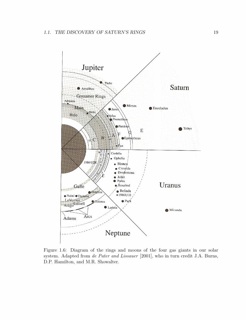
More than 350 years after Galileo’s 1610 observations, Saturn was thought to be
the only planet in our solar system to have a ring system. Then in 1977, rings were
detected at Uranus during a stellar occultation of the star SAO 158687 [Elliot et al.,
1977]. Two years later in 1979, Voyager 1 detected faint rings around Jupiter [Smith
et al., 1979]. And in 1981, Neptune’s “ring arcs” were observed during another stellar
occultation, though originally misinterpreted as being due to a chance occultation
by a new satellite [Reitsema et al., 1982; Nicholson et al., 1990]. In a matter of a
few short years, ring systems went from being unique to Saturn, to being a common
feature of the gas giants in our solar system. Each planet has fundamentally different
ring systems (see Figure 1.6), the reason for which is still a matter of scientific debate
[Burns , 1999].

18 CHAPTER 1. INTRODUCTION AND HISTORICAL REVIEW
Table 1.1: Key milestones in the study of Saturn’s rings
Date Event
1543 Copernicus proposes that the Earth and other planets orbit the Sun1608 The modern telescope is invented1609 Kepler publishes the first two of his three laws of motion in Astronomia
Nova1610 Galileo observes the rings of Saturn1612 Galileo observes the rings’ disappearance1616 The rings appear as handles, or ‘ansae’1656 Huygens correctly describes the rings as an annulus1657 Pendulum clock is invented1659 Huygens publishes Systema Saturnium1660 The Royal Society is founded in London1676 Cassini observes his eponymous division1687 Newton publishes Principia1787 Laplace proposes many thin solid ring theory1791 Herschel supports two solid ring theory1821 Faraday invents the electric motor1826 The internal combustion engine is invented1857 Maxwell proves the rings must be composed of particles1859 Darwin’s On the Origin of Species is published1872 Kirkwood proves that observed ring features are caused by resonances with
moons1873 Maxwell’s A Treatise on Electricity and Magnetism is published1895 Keeler verifies Maxwell’s many-particle theory experimentally1902 First trans-atlantic radio transmission (Marconi)1903 First powered flight of an airplane (Wright brothers)1967 Ring E is discovered1970 Spectroscopic observations reveal that the rings are composed primarily of
water ice1978 The existence of density waves in the rings is proposed by Goldreich and
Tremaine1979 Ring F is discovered by the Pioneer spacecraft imaging team1980 Voyager 1 performs the first radio occultation of Saturn’s rings1980 Ring D is discovered1981 Lissauer proposes that moonlets are embedded within Saturn’s ring system1990 The Hubble Space Telescope is deployed to Earth orbit by the Space Shuttle
(STS-31)1997 The Cassini/Huygens spacecraft is launched from Cape Canaveral2004 Cassini/Huygens is inserted into Saturn orbit
1.1. THE DISCOVERY OF SATURN’S RINGS 19
Figure 1.6: Diagram of the rings and moons of the four gas giants in our solarsystem. Adapted from de Pater and Lissauer [2001], who in turn credit J.A. Burns,D.P. Hamilton, and M.R. Showalter.

20 CHAPTER 1. INTRODUCTION AND HISTORICAL REVIEW
1.2 Occultation Studies of Saturn’s Rings: A Brief
History
Much of what is known about the radial structure in Saturn’s rings has been derived
from occultation experiments. Occultation experiments are made when the line-
of-sight path between a transmitter and a receiver intercept or ‘occult’ an object
under study, be that an atmosphere or a planetary ring system. In the case of
stellar occultation, the transmitter is a star, and the receiver is an instrument that
collects radiant stellar energy over a particular range of wavelengths in the star’s
electromagnetic spectrum. In the case of radio occultation, the transmitter and the
receiver are radio instruments designed and built to the specifications required to
conduct the experiment.
The primary measurement of occultation experiments is the apparent opacity, or
optical depth τ , of the rings to electromagnetic waves of a particular wavelength. If
the rings are illuminated with an incident electromagnetic wave of intensity Io, and
the intensity just behind the rings is I, the oblique optical depth τq is defined as,
τq = − ln (I/Io) (1.1)
Normal optical depth τ is related to the oblique optical depth by,
τ = µoτq (1.2)
where µo = sinB is the sine of the ring opening angle B, which is the angle that the
wave vector k of the incident light makes with the ring plane (i.e., if B = 90o then
k is normal to the plane of the rings). Methods for estimating optical depth from
radio occultation measurements are discussed in detail in Appendix A.1. A detailed
description of the geometry of the Cassini radio occultation experiments is provided
in Chapter 4.
Stellar occultations conducted using the Voyager spacecraft’s ultraviolet spectrom-
eter (UVS) [Sandel et al., 1982; Holberg et al., 1982] and photopolarimeter subsystem
(PPS) [Esposito et al., 1983, 1987] observed the occultation of the star δ Sco (located

1.2. OCCULTATION STUDIES OF SATURN’S RINGS: A BRIEF HISTORY 21
in the constellation Scorpius) at 0.11- and 0.27-µm wavelengths, respectively, provid-
ing optical depth profiles of the rings with sampling resolutions of 0.1 and 3.2 km,
respectively. Ground-based observations of the ring occultation of the star 28 Sgr
were used by Nicholson et al. [2000] to derive optical depth profiles at 0.9, 2.1, 3.3,
and 3.9 µm wavelengths, and were used in conjunction with the PPS δ Sco occultation
result to estimate the number distribution of particles of radii ranging from 0.3–20
meters [French and Nicholson, 2000]. More recently, the visual and infared mapping
spectrometer (VIMS) and the ultraviolet imaging spectrograph (UVIS) instruments
onboard NASA’s Cassini spacecraft are currently being used to conduct multiple stel-
lar occultations of the Saturnian rings, yielding a dataset that is now being gathered
and analyzed (e.g., Nicholson et al. [2007]; Colwell and Esposito [2007]).
Radio occultation in particular has proven to be a valuable experimental method
for probing planetary rings. The technique was first applied to rings during the
Voyager 1 flyby of Jupiter on March 5, 1979. Although that particular experiment
was unable to detect Jupiter’s tenuous rings, the non-detection allowed scientists to
establish bounds on the optical depth and particle sizes [Tyler et al., 1981]. The
Jovian encounter was followed by the great successes of Voyager 1’s flyby encounter
with Saturn in 1980, and Voyager 2’s flyby of Uranus in 1986.
At Saturn, Voyager 1’s radio science subsystem (RSS) simultaneously probed the
rings at 3.6- and 13-cm wavelengths, yielding diffraction-corrected optical depth pro-
files with resolutions approaching 200 meters in regions of Ring C, and with 400-meter
resolution over the full extent of the rings [Tyler et al., 1983; Marouf et al., 1986].
Estimates of ring particle size distributions, local ring thickness, and the degree of
particle crowding derive from the radio occultation data, for assumed many particles
thick (MPT) ring models [Marouf et al., 1982, 1983] and for thin finite number of
layers (FNL) ring models [Zebker and Tyler , 1984; Zebker et al., 1985]. We describe
these models in greater detail in Appendix A.
At Uranus, the large ring opening angle of B = 81.5o facilitated a high signal-
to-noise ratio (SNR) radio occultation of the rings. All nine of the rings that were
known prior to Voyager were detected in the radio data. The high SNR of these
measurements made it possible to reconstruct the optical depth profiles of the rings

22 CHAPTER 1. INTRODUCTION AND HISTORICAL REVIEW
at resolutions as fine as 50 meters [Tyler et al., 1986; Gresh et al., 1989].
An attempt was made to observe Neptune’s rings with Voyager 2 in 1989, but
this was not successful. Neptune’s rings form incomplete arcs of material, and the
spacecraft trajectory did not allow for an occultation measurement of any of these
arcs.
The first extensive radio occultation study of a ring system using an orbiting
spacecraft is currently underway at Saturn using the RSS onboard NASA’s Cassini
spacecraft. In contrast to the hyperbolic flyby trajectories of Voyager, Cassini is an
orbiter dedicated to the observation of Saturn, its moons, and its rings. Cassini was
inserted into orbit around Saturn on July 1, 2004, and its nominal mission (July
2004 - August 2008) consisted of 75 orbits, during which 20 radio occultations of
the rings were performed over a range of observational geometries. Four of these
20 occultations comprise both ingress and egress observations, while the remaining
16 occultations are single-sided (either ingress or egress), for a total of 24 distinct
observations. An extended Cassini mission plan was approved by NASA, consisting
of a further 60 orbits which took place between July 2008 and July 2010. In February
of 2010, NASA announced its plans to extend funding and support for the Cassini
mission until 2017.
1.3 Contents and Contributions of this Disserta-
tion
This dissertation focusses on the work done between early 2004 and June of 2008 to
estimate the fine-scale structure of Saturn’s rings. Contributions made outside of this
area have been included as appendices, as described at the end of this chapter.
We present here a forward-theoretic modeling approach which we use to produce
estimates of the key physical dimensions of small-scale microstructure in Saturn’s
rings, at length scales of one to several hundreds of meters. We define microstructure
as an anisotropic distribution of ring particles to form clusters or groupings that con-
stitute discernible patterns. In particular, we focus on highly periodic, axisymmetric
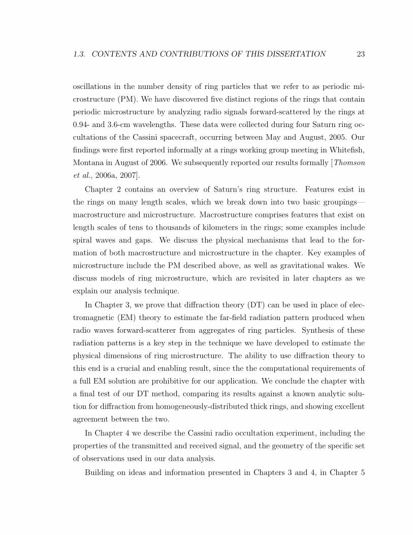
1.3. CONTENTS AND CONTRIBUTIONS OF THIS DISSERTATION 23
oscillations in the number density of ring particles that we refer to as periodic mi-
crostructure (PM). We have discovered five distinct regions of the rings that contain
periodic microstructure by analyzing radio signals forward-scattered by the rings at
0.94- and 3.6-cm wavelengths. These data were collected during four Saturn ring oc-
cultations of the Cassini spacecraft, occurring between May and August, 2005. Our
findings were first reported informally at a rings working group meeting in Whitefish,
Montana in August of 2006. We subsequently reported our results formally [Thomson
et al., 2006a, 2007].
Chapter 2 contains an overview of Saturn’s ring structure. Features exist in
the rings on many length scales, which we break down into two basic groupings—
macrostructure and microstructure. Macrostructure comprises features that exist on
length scales of tens to thousands of kilometers in the rings; some examples include
spiral waves and gaps. We discuss the physical mechanisms that lead to the for-
mation of both macrostructure and microstructure in the chapter. Key examples of
microstructure include the PM described above, as well as gravitational wakes. We
discuss models of ring microstructure, which are revisited in later chapters as we
explain our analysis technique.
In Chapter 3, we prove that diffraction theory (DT) can be used in place of elec-
tromagnetic (EM) theory to estimate the far-field radiation pattern produced when
radio waves forward-scatterer from aggregates of ring particles. Synthesis of these
radiation patterns is a key step in the technique we have developed to estimate the
physical dimensions of ring microstructure. The ability to use diffraction theory to
this end is a crucial and enabling result, since the the computational requirements of
a full EM solution are prohibitive for our application. We conclude the chapter with
a final test of our DT method, comparing its results against a known analytic solu-
tion for diffraction from homogeneously-distributed thick rings, and showing excellent
agreement between the two.
In Chapter 4 we describe the Cassini radio occultation experiment, including the
properties of the transmitted and received signal, and the geometry of the specific set
of observations used in our data analysis.
Building on ideas and information presented in Chapters 3 and 4, in Chapter 5

24 CHAPTER 1. INTRODUCTION AND HISTORICAL REVIEW
we define the set of tools and procedures we used to extract estimates of the physical
dimensions of PM from Cassini signals.
In Chapter 6, we present experimental evidence for the presence of PM in the
rings. We apply the techniques described in Chapter 5 to our data, reporting esti-
mates of the location, structural period, and orientation of these PM features. We
compute estimates using two different model types to represent PM, and show con-
sistent results. We briefly review a phenomenon known as viscous overstability, and
examine its potential to explain the presence of PM in some regions of the rings.
Chapter 7 contains a summary of the key findings presented in this dissertation,
along with a discussion of some important open questions and some suggestions for
future work.
A summary of the major contributions of this work are:
1. We uncovered five distinct locations in Saturn’s rings A and B exhibiting highly
periodic, fine-scale variation in the ring optical depth. The physical period of
these variations range between 100–250 meters [Thomson et al., 2007].
2. An exhaustive study, comparing the results of a multiple scattering formulation
of Mie theory against the results of scalar diffraction theory. The study, which
examined 2-, 3-, and 10-sphere clusters of particles, shows that diffraction theory
accurately predicts the far-field scattering pattern of particle aggregates, as long
as the region of interest is limited to electrically large particles scattering in the
near-forward direction [Thomson and Marouf , 2009].
3. Derivation of the exact solution for the five-term power-law expression of Al-
lan variance, showing that the exact solution and the well-known approximate
solution converge very quickly; i.e., the approximate form is sufficient and sat-
isfied by most imaginable measurement conditions [Thomson et al., 2005]. An
adaptation of this paper is included as Appendix D.
4. Demonstration of the equivalence of the Radon and Abel Transforms, as they
are applied in atmospheric radio occultation [Thomson and Tyler , 2007]. An
adaptation of this paper is included as Appendix E.

1.3. CONTENTS AND CONTRIBUTIONS OF THIS DISSERTATION 25
In this dissertation, we attempt to conform to the variable naming conventions
established a priori in the literature to the greatest extent possible. This inevitably
leads to some overlap in the use of variables, since the work contained herein spans
several fields—electromagnetics, optics, remote sensing, and planetary science. We
explicitly describe variable assignments throughout the dissertation to minimize po-
tential confusion. The reader is referred to the List of Symbols provided in the preface
material for a complete list of all symbol assignments used in this dissertation.

26 CHAPTER 1. INTRODUCTION AND HISTORICAL REVIEW
Chapter 2
Saturn Ring Structure and
Dynamics
The basic structure of Saturn’s rings is depicted in Figure 2.1. Rings A, B, and C
(and the Cassini Division, which separates Ring A from B) are collectively known
as Saturn’s main rings or the classical ring system. Interior to the main rings is
the D ring, which was discovered by a combination of Voyager observations and a
single ground-based stellar occultation [Hedman et al., 2007]. From the inner edge
of Ring D to the outer edge of Ring A the rings extend radially for 69,875 km, from
approximately 66,900 km to 136,775 km from Saturn’s center, or 1.110Rs through
2.269Rs, where Rs = 60, 268 km is the equatorial radius (at the 1 bar atmospheric
pressure level) of Saturn. The main rings are thought to be on the order of 10–20
meters thick [Deau et al., 2008; Charnoz et al., 2009]. Exterior to the main rings, the
narrow and braided Ring F is centered at 140,180 km (2.326Rs); and the tenuous G
and E rings lie between 170,000–175,000 km (2.82Rs–2.90Rs) and between 181,000–
483,000 km (3.00Rs–8.01Rs), respectively. Ring G is composed primarily of dust
[Cuzzi et al., 2009], while Ring E is composed primarily of water ice [Hillier et al.,
2007].
In 2009 the Phoebe ring was discovered [Verbiscer et al., 2009], an 80Rs-thick band
of dust spanning 3.5 × 10⁶–1.8 × 10⁷ km (59Rs–300Rs), and is thought to comprise
ejecta resulting from meteoroid impacts on the Saturnian moon Phoebe. The Phoebe
27

28 CHAPTER 2. SATURN RING STRUCTURE AND DYNAMICS
ring is in the solar system ecliptic, inclined by about 27o with the other rings, and
its particles likely orbit Saturn in retrograde, similar to Phoebe. A comprehensive
description of the rings is included in Dougherty [2009]. Properties of the various ring
regions are summarized in Table 2.1.
Saturn’s main rings comprise particles of predominantly crystalline water ice,
mixed with impurities that give the rings a slight reddish color [Cuzzi et al., 2009].
Particle sizes range from motes of dust to small moons [Cuzzi et al., 2009; Charnoz
et al., 2009]. Figure 2.3 is a false-color image of the rings produced from radio occul-
tation data using techniques described in Section A.2. Colors in the figure indicate
which range of ring particle sizes is predominant locally in the population, as described
in the figure caption.

29
(a)Structure
ofSaturn’s
ringsystem
(b)Comparisonof
theopacity
ofSaturn’s
main
ringsatopticalan
dradio
wavelengths.
Inboth
images,brightnessindicatesgreater
opticaldepth.
Figure
2.1:
Structure
ofSaturn’s
rings.(a)an
d(b)arePIA
03550an
dPIA
07874,
respectively,from
theNASA
Photojournal
website.See
Tab
le2.1forasummaryof
thelocation
ofthevariou
sringregion
srelative
toSaturn’s
centerof
mass.
30 CHAPTER 2. SATURN RING STRUCTURE AND DYNAMICS
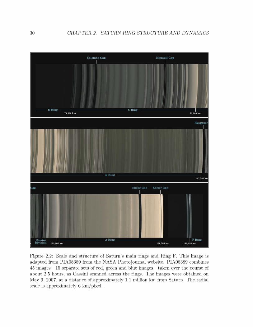
Figure 2.2: Scale and structure of Saturn’s main rings and Ring F. This image isadapted from PIA08389 from the NASA Photojournal website. PIA08389 combines45 images—15 separate sets of red, green and blue images—taken over the course ofabout 2.5 hours, as Cassini scanned across the rings. The images were obtained onMay 9, 2007, at a distance of approximately 1.1 million km from Saturn. The radialscale is approximately 6 km/pixel.

31
Figure 2.3: Particle size distributions in Saturn’s Cassini Division and Ring A. Thisimage was constructed from optical depth profiles produced at three radio wavelengths(0.94, 3.6, and 13 centimeters, or Ka-, X-, and S-bands, respectively). The structuralresolution is about 10 kilometers. Shades of red indicate an absence of particles lessthan 5 centimeters in diameter. Green and blue shades indicate regions where thereare particles of sizes smaller than 5 centimeters and 1 centimeter present, respectively.A color shift from red to blue indicates an increase in the relative abundance of smaller(< 5 cm) sized particles. The image indicates a general increase in the population ofthese small particles with radial distance, from inner to outer Ring A. The deep blueshades in the vicinity of the Keeler gap (the narrow dark band near the edge of ringA) indicate an increased abundance of even smaller particles, of diameter less than acentimeter. It is thought that frequent collisions between large ring particles in thisdynamically active region likely fragment the larger particles into more numeroussmaller ones. Image is PIA07960, NASA Photojournal website.

32 CHAPTER 2. SATURN RING STRUCTURE AND DYNAMICS
Tab
le2.1:
Properties
ofSaturn’sRingSystem
.Adap
tedfrom
dePater
andLissauer
[2001].
Main
rings
Dring
Cring
Bring
Cassini
division
Aring
Fring
Gring
Ering
Phoeb
ering
Radial
location
(Rs)
1.09–
1.24
1.24–
1.53
1.53–
1.95
1.95–
2.03
2.03–
2.27
2.32
2.75–
2.87
3–8
59–
300?
Vertical
thickness
<1km
<1km
<1km
103–
2×
104
km
a
4.8×
106km
Norm
al
optical
dep
th
≈ 10−5
–10
−4
0.05–
0.2
1–3
0.1–0.15
0.4–1
110
−5–
10−4
10−7
–10
−6??
Particle
size
µm
mm–m
cm–10
mcm
–10m
cm–10
mµm–cm
µm–
cm?
1µm
b??
aIncreaseswithradiallocation
bVerynarrow
distribution

2.1. RING MACROSTRUCTURE 33
2.1 Ring Macrostructure
If the only forces acting on planetary ring particles were the gravitational pull of
the host planet and inter-particle collisional forces, then all planetary ring systems
would evolve over time into thin, featureless discs. Perturbations due to the gravita-
tional influence of moons external and internal to the rings act in conjunction with
self-gravitational effects to produce large-scale features—or macrostructure—in the
rings. Some examples of ring macrostructure include ring divisions, gaps, waves, and
edges. These features exist throughout Saturn’s main rings, on length scales of tens
to thousands of kilometers.
Ring particles having orbital frequency n(r) that are perturbed from circular or-
bits will oscillate freely about their reference circular orbit with epicyclic (radial)
frequency κ(r) and vertical frequency µ(r). The gravitational consequences of Sat-
urn’s oblateness cause a separation of these frequencies, µ(r) > n(r) > κ(r), and
thus the radial location of the vertical and horizontal resonances associated with a
particular moon are different. Ring particles orbiting at or near these resonance loca-
tions experience coherent ‘kicks’, which over time can contribute to significant forced
oscillations (e.g., de Pater and Lissauer [2001]).
Resonant forcing of particles in the rings by moons external to a particular ring
location can create two main types of ring macrostructure: gaps or ring boundaries,
and spiral density or bending waves [Cuzzi et al., 1984; Rosen, 1989; de Pater and
Lissauer , 2001]. These features are generated by torques that transport angular mo-
mentum between the resonant moon(s) and ring material. The disturbance (forcing)
frequency due to the influence of a particular moon is given by,
ωf = mθns ±mzµs ±mrκs (2.1)
where the subscript s indicates that ωf is tied to a specific satellite s, and mθ, mz, and
mr are non-negative integers with mz odd for vertical forcing and even for horizontal
forcing [de Pater and Lissauer , 2001]. A horizontal resonance condition, also known

34 CHAPTER 2. SATURN RING STRUCTURE AND DYNAMICS
as a Lindblad resonance, occurs at the radial location r = rL when,
ωf −mθn(rL) = ±κ(rL) (2.2)
Vertical resonances are excited at r = rv if,
ωf −mθn(rv) = ±µ(rv) (2.3)
Eq. (2.2) yields two possible solutions for rL; we refer to the lesser (greater) of these
as the inner (outer) Lindblad resonance. Similarly, eq. (2.3) yields an inner and outer
vertical resonance. The oblateness of Saturn ensures that rL > rv for resonances
excited by a given moon.
Specific resonances are identified by the ratio,
n(rv,L)
ns
≈ mθ +mz +mr
mθ − 1=
l
mθ − 1(2.4)
The strongest horizontal resonances have mz = mr = 0, while the strongest vertical
resonances have mz = 1, mr = 0. By convention, it is common to reference a
resonance by its ratio, written as l : (mθ − 1).
2.1.1 Gaps and Ring Boundaries
Lindblad resonances are responsible for the creation of sharply defined, non-circular
ring boundaries. The outer edge of Ring B is coincident with the 2:1 inner Lindblad
resonance (ILR) of the moon Mimas, generating an oval boundary that co-rotates with
Mimas. Ring A’s outer boundary corresponds to the 7:6 resonance of the coorbital
moons Janus and Epimetheus, and has a seven-lobed boundary. To create a sharp
edge/boundary in the rings or to maintain a ring gap, a resonance must exert sufficient
torque on the rings to offset the localized viscous spreading of ring material.
Gaps in the rings are created by the same process that creates edges. In the
optically thin Ring C, resonances are responsible for the creation of many gaps, often
accompanied by optically thicker ringlets. Gap formation requires more force in the

2.1. RING MACROSTRUCTURE 35
(a) Image PIA06237, NASA Photojournal website.
(b) Image PIA11653, NASA Photojournal website.
Figure 2.4: The Keeler Gap and its shepherding moon Daphnis. (a) Daphnis occupiesan inclined orbit within the 42-km wide Keeler Gap. Torques exerted by the moonon ring particles as they move past the moon (moving left-right in this figure) createhorizontal and vertical ripples on the inner and outer gap edges. Resolution is 3km/pixel. (b) The small sun-ring plane angle in this mid-August 2009 Saturn equinoximage causes out-of-plane structures to cast long shadows across the rings. Thevertical structure of the Keeler Gap edges and the out-of-plane position of Daphnisare captured. Gap edges are 0.5–1.5-km tall; approximately 50–150 times taller thanthe average ring thickness. Resolution is 5 km/pixel.
36 CHAPTER 2. SATURN RING STRUCTURE AND DYNAMICS
(a) Image PIA07587, NASA Photojournal web-site.
(b) Image PIA06093, NASA Photojournal web-site.
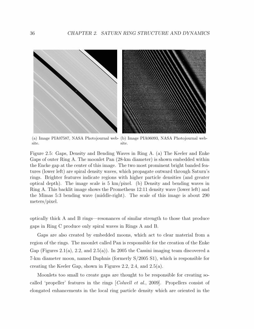
Figure 2.5: Gaps, Density and Bending Waves in Ring A. (a) The Keeler and EnkeGaps of outer Ring A. The moonlet Pan (28-km diameter) is shown embedded withinthe Encke gap at the center of this image. The two most prominent bright banded fea-tures (lower left) are spiral density waves, which propagate outward through Saturn’srings. Brighter features indicate regions with higher particle densities (and greateroptical depth). The image scale is 5 km/pixel. (b) Density and bending waves inRing A. This backlit image shows the Prometheus 12:11 density wave (lower left) andthe Mimas 5:3 bending wave (middle-right). The scale of this image is about 290meters/pixel.
optically thick A and B rings—resonances of similar strength to those that produce
gaps in Ring C produce only spiral waves in Rings A and B.
Gaps are also created by embedded moons, which act to clear material from a
region of the rings. The moonlet called Pan is responsible for the creation of the Enke
Gap (Figures 2.1(a), 2.2, and 2.5(a)). In 2005 the Cassini imaging team discovered a
7-km diameter moon, named Daphnis (formerly S/2005 S1), which is responsible for
creating the Keeler Gap, shown in Figures 2.2, 2.4, and 2.5(a).
Moonlets too small to create gaps are thought to be responsible for creating so-
called ‘propeller’ features in the rings [Colwell et al., 2009]. Propellers consist of
elongated enhancements in the local ring particle density which are oriented in the
2.1. RING MACROSTRUCTURE 37
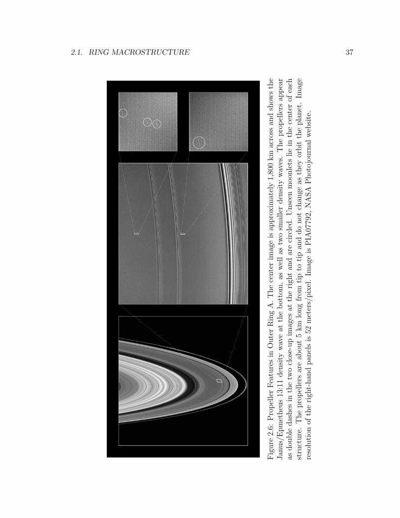
Figure
2.6:
PropellerFeaturesin
OuterRingA.Thecenterim
ageisap
proxim
ately1,800km
across
andshow
sthe
Jan
us/Epmetheus13:11density
waveat
thebottom,as
wellas
twosm
allerdensity
waves.Thepropellers
appear
asdou
ble
dashes
inthetw
oclose-upim
ages
attherigh
tan
darecircled.Unseen
moon
lets
liein
thecenterof
each
structure.Thepropellers
areab
out5km
longfrom
tipto
tipan
ddonot
chan
geas
they
orbittheplanet.Im
age
resolution
oftherigh
t-han
dpan
elsis52
meters/pixel.Im
ageisPIA
07792,
NASA
Photojournal
website.

38 CHAPTER 2. SATURN RING STRUCTURE AND DYNAMICS
direction of orbital motion and extend for several kilometers from tip-to-tip. Pro-
pellers can also open local ring gaps. The moonlets responsible for the propeller
features shown in Figure 2.6 are thought to be on the order of 40–500 meters in
diameter (compare with the 7-km diameter of Daphnis) [Tiscareno et al., 2008].
2.1.2 Spiral Density and Bending Waves
Spiral bending and density waves propagate from all of the strong satellite resonance
locations in the rings, when the torques exerted on ring material by the resonance are
insufficient to transport material away and maintain edges or gaps. Spiral waves are
seen broadly throughout Ring A, and are the cause of the prominent optical depth
variations visible in Figures 2.4, 2.5, and 2.6.
Density waves manifest as an in-plane compression and rarefaction of the local
number density of ring particles, originating at Lindblad resonance locations in the
ring plane. Similarly, bending waves are excited at vertical resonance locations, where
the satellite resonance induces small inclinations in the local orbits of ring particles.
The resulting vertical excursions (of up to ∼400 meters [de Pater and Lissauer ,
2001]) or undulations of particles about the ring plane gives the rings a corrugated
appearance. For both density and bending waves, the self-gravity of particles within
the ring disk provides the restoring force that allows waves to propagate away from
the origin of the resonant disturbance. Rosen [1989] produced an excellent visual
depiction of density and bending waves, reproduced here in Figure 2.7. The self-
gravity of the ring particles effectively distributes the torque applied by the resonant
satellite, from particles at rL or rv to adjacent particles. Waves are the mechanism by
which resonant forcing energy diffuses away from the disturbance. Density waves are
excited at the ILR of the resonant satellite, and propagate towards Saturn. Bending
waves are excited at the inner vertical resonance (IVR), and propagate outward in
the rings away from Saturn, except for so-called nodal bending waves, mθ = 1, which
propagate towards Saturn. For all spiral waves, the number of spiral arms created is
equal to mθ.

2.1. RING MACROSTRUCTURE 39
Figure 2.7: Schematic of density and bending waves, showing a probing radio ray.From Rosen [1989].

40 CHAPTER 2. SATURN RING STRUCTURE AND DYNAMICS
2.2 Ring Microstructure
Small scale structures in the rings, which we denote ring microstructure, form as a re-
sult of the influence of inter-particle gravitational and collisional forces, in the presence
of the ‘background’ gravitational forces at play locally. We define microstructure as a
discernible organization of ring particles into groups or clusters, with length scales on
the order of tens to several hundreds of meters. Although the relevant length scales of
microstructure itself are as described, a region containing microstructure may extend
over tens or thousands of kilometers within the rings. Notable examples of distinctive
microstructure include gravitational wakes, and periodic microstructure (PM).
2.2.1 Gravitational Wakes
Dynamical simulations of planetary rings predict that the interplay of collisional and
gravitational forces produces gravitational wakes broadly within Saturn’s main rings
[Salo, 1992, 1995; Tiscareno et al., 2009; Dougherty , 2009]. Observed optical depth
variations with ring longitude in Saturn’s Rings A and B—a phenomenon known as
azimuthal asymmetry—provide indirect evidence for the existence of gravitational
wakes [Salo et al., 2004; Colwell et al., 2006; French et al., 2007; Dougherty , 2009].
Wakes form in the rings at cant angles of 20o–25o to the local azimuthal unit
vector. For particles in circular orbits, this is also the local particle velocity unit
vector. The cant angle is determined by particle self-gravity in combination with the
local Keplerian shear, which is the sliding of local, radially adjacent ring particles past
each other due to their differing orbital velocities (the orbital velocity of particles in
circular orbits is proportional to√
1/r, where r is the radial distance of an orbiting
particle from Saturn’s center of mass). Wakes are ephemeral structures, constantly
being pulled apart by Keplerian shear and re-formed by self-gravity. Although their
specific composition is in a state of flux, the wake structure remains constant in a
statistical sense, as long as the local physical conditions (particle composition, size
distribution, density, etc.) remain relatively constant. Figure 2.8 is a snapshot from a
dynamical simulation [Salo, 2006] revealing the characteristic pseudo-periodicity and
canting typical of gravitational wakes.
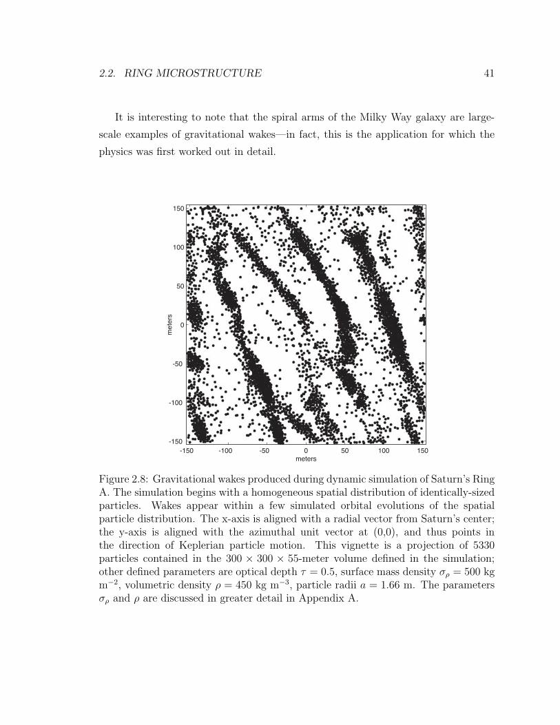
2.2. RING MICROSTRUCTURE 41
It is interesting to note that the spiral arms of the Milky Way galaxy are large-
scale examples of gravitational wakes—in fact, this is the application for which the
physics was first worked out in detail.
meters
met
ers
-150 -100 -50 0 50 100 150-150
-100
-50
0
50
100
150
Figure 2.8: Gravitational wakes produced during dynamic simulation of Saturn’s RingA. The simulation begins with a homogeneous spatial distribution of identically-sizedparticles. Wakes appear within a few simulated orbital evolutions of the spatialparticle distribution. The x-axis is aligned with a radial vector from Saturn’s center;the y-axis is aligned with the azimuthal unit vector at (0,0), and thus points inthe direction of Keplerian particle motion. This vignette is a projection of 5330particles contained in the 300 × 300 × 55-meter volume defined in the simulation;other defined parameters are optical depth τ = 0.5, surface mass density σρ = 500 kgm−2, volumetric density ρ = 450 kg m−3, particle radii a = 1.66 m. The parametersσρ and ρ are discussed in greater detail in Appendix A.

42 CHAPTER 2. SATURN RING STRUCTURE AND DYNAMICS
2.2.2 Periodic Microstructure
In addition to the formation of wakes, the dynamical theory of the rings predicts the
formation of stable regions of regular, azimuthally-symmetric density fluctuations on
the scale of tens to hundreds of meters. The incipient condition believed to be respon-
sible for these structures is known as viscous overstability (VO), a linear instability
that occurs when the viscous stresses vary with number density in such a way that Ke-
plerian shear energy reinforces and promotes growing density oscillations [Latter and
Ogilvie, 2008]. Linear dynamical theory predicts the onset of these density oscilla-
tions, and non-linear dynamical theory predicts that the density oscillations saturate
most strongly at length scales of 100–200 meters. Simulations by Schmit [Schmit and
Tscharnuter , 1999; Schmidt et al., 2001] and others have produced instantiations of
fine-scale PM due to viscous overstability; see Figure 2.9. Although Schmidt et al.
[2001] focus on Ring B, the environmental conditions necessary to support stable VO
regions exist in parts of Ring A as well (see Chapter 6 for a more detailed discussion).
Using the Cassini radio occultation experiment, we have directly observed fine-scale
PM in Ring A consistent with the density fluctuations predicted by the saturated
state of viscous overstability. Reporting those discoveries constitutes the primary
objective of this dissertation.

2.2. RING MICROSTRUCTURE 43
meters
met
ers
Figure 2.9: Dynamical simulations of the rings reported in Schmidt et al. [2001]produce fine-scale periodic microstructure due to viscous overstability (VO), withlength scales on the order of 100 meters. The x- and y-axis alignment is as describedin Figure 2.8, with simulated optical depth τ = 1, particle radii a = 1 meter. Point(0,0) is centered at a distance 100,000 km from Saturn’s center, corresponding toinner Ring B (see Figure 2.2).
Figure 2.10: Artist Marty Peterson’s rendition of the fine-scale composition and struc-ture of Saturn’s rings, based on a 1983 illustration by William K. Hartmann. Thelargest individual particles shown are a few meters across. Image PIA10081, NASAPhotojournal website.

44 CHAPTER 2. SATURN RING STRUCTURE AND DYNAMICS
2.3 Models of Ring Microstructure
The interplay of forces discussed in Section 2.2 give rise to a broad range of possible
microstructure in the rings. To illustrate this, we present a survey of dynamical sim-
ulation results for Saturn’s rings in Figure 2.11. Here, simulations are parameterized
along two axes: the optical depth τ of the rings, and a ratio rh which characterizes the
importance of self-gravity relative to Saturn’s tidal force (e.g., Schmidt et al. [2009]),
rh =RHill
a1 + a2=
[(m1 +m2)
3Ms
]1/3ro
a1 + a2
=
(ρo3ρs
)1/3(roRs
)(1 +m1/m2)
1/3
1 + (m1/m2)1/3(2.5)
RHill is the mutual Hill radius for a pair of particles of radius a1 and a2, having masses
m1 and m2 and density ρo, ro is the radial location of the particles relative to Saturn’s
center of mass, and ρs and Rs are the mean density and radius of Saturn. Simula-
tions shown in Figure 2.11 assume that ring particles have a normal coefficient of
restitution—defined as the ratio of post-collisional to pre-collisional normal velocities
of two colliding particles—of εn = 0.5. εn is velocity and mass dependent, is sensitive
to the mechanical and surface properties of the colliding particles, and can strongly
affect the microstructure regimes predicted by dynamical simulations; see Schmidt
et al. [2009] for more details.
Where self-gravity dominates tidal forces, simulations show that ring particles ag-
gregate into clumps. Where self-gravity effects are relatively small and the optical
depth is not too great, populations tend towards homogeneous ring particle distribu-
tions. Gravitational wakes can form throughout much of the remaining simulation
space, including regions where viscous overstability produces axisymmetric density
oscillations as well. In these simulations, the conditions for the onset of overstable
oscillations are approximately τ > 1, rh < 0.6.
In this dissertation, we develop a method for estimating the physical dimensions of
microstructure in Saturn’s rings by fitting the diffraction signature of various physical
ring models to diffraction features contained in signals received from the Cassini

2.3. MODELS OF RING MICROSTRUCTURE 45
ro
Figure 2.11: A survey of ring microstructure, showing dependence on normal opticaldepth τ and on the strength of self-gravity relative to tidal forces, quantified by theparameter rh (see text). The distance ro from Saturn’s center is indicated, pairedwith the corresponding value of rh when ρo = 900 kg m−3 (i.e., consistent with thedensity of water ice). The simulation space comprises identical particles with coeffi-cient of restitution εn = 0.5. The figure insert shows a schematic of the regions in rh-τspace where different physical processes control the nature of the ring microstructurethat is shown in the main plot. Indicated physical processes are collisional (impacts),pairwise-gravitational (encounters), self-gravitational (aggregates), and a combina-tion of self-gravitational and tidal (wakes). Note that in the upper left region of theplot, τ > 1, rh < 0.6, axisymmetric overstable oscillations coexist with gravitationalwakes in the simulation. Adapted from Schmidt et al. [2009].

46 CHAPTER 2. SATURN RING STRUCTURE AND DYNAMICS
meters-100 -50 0 50 100
met
ers
150
100
50
0
-50
-100
-150
meters-150 -100 -50 0 50 100
meters-100 -50 0 50 100 150
(a) (b) (c)
Figure 2.12: Models of ring microstructure. The three panels each contain 5330 3.32-meter diameter particles filling a 300m×300m×55m volume. Populations representmodels of (a) homogeneously distributed thick rings, (b) gravitational wakes, and (c)periodic microstructure.
spacecraft during multiple radio occultation observations. To this end, we introduce
four microstructure models for use in the fitting process:
1. Homogeneously distributed thick rings
2. Packed (i.e., crowded) monolayers
3. Gravitational wakes
4. Periodic microstructure (PM)
Examples of homogeneous, wake, and PM ring models are shown in Figure 2.12.
Packed monolayers are predicted by some ring theorists, who contend that collisional
processes drive an evolution towards dynamically ‘cold’ rings comprising a single layer
of relatively large particles, surrounded by a cloud of smaller particles [Deau et al.,
2008]. Monolayer distributions have been proposed by some researchers to explain
evidence of non-homogeneous ring particle distributions seen in radio occultation data
(e.g., see Figures 4.5E and 5.1). Clumped microstructure is not modeled, since Cassini
signals show no evidence of microstructure in regions where clumping is predicted by
dynamical simulations.
The use and parameterization of these models is described in detail in Chapter 5.

2.4. SUMMARY 47
2.4 Summary
The dynamical interplay of collisional and gravitational forces produces fine-scale
structure in Saturn’s rings, manifesting as anisotropic particle distributions. Ob-
servations provide evidence for the existence of gravitational or density wakes [Salo
et al., 2004], axisymmetric periodic microstructure [Colwell et al., 2007; Thomson
et al., 2007], and rarified homogeneous particle distributions. Clumped distributions
have been shown to be possible theoretically in computer models of planetary rings,
e.g., Salo [1992, 1995], but so far have not been observed experimentally in any con-
clusive way.
In Chapter 3, we examine the electromagnetic (EM) scattering properties of ag-
gregates of icy ring particles. That analysis plays a key role in our treatment of the
Cassini radio occultation experiment (which we describe in detail in Chapter 4), since
a major component of the received Cassini signal is forward-scattered from ring par-
ticles to receivers on Earth. We show that for the purposes of our experiment, a full
EM solution is not required to accurately predict the forward scattering behavior of
ring microstructure. Rather, we show that a diffraction theoretic approach produces
accurate, predictive results that closely mimic the results of EM theory, while greatly
reducing the complexity of the forward scattering model.

48 CHAPTER 2. SATURN RING STRUCTURE AND DYNAMICS
Chapter 3
EM Scattering and Diffraction
from Ring Particle Clusters
Small-scale structure in Saturn’s rings is evident in signals received during Cassini
radio occultation observations. During those observations—which are described in
detail in Chapter 4—individual particles forward-scatter radio signals from within a
region of the rings illuminated by Cassini’s high-gain antenna. A small but detectible
fraction of that scattered energy propagates along the near-forward or paraxial direc-
tion, and is received by antennas belonging to NASA’s Deep Space Network (DSN).
Superimposed on the scattered signal is the diffraction signature of the arrangement
of those particles in the ring plane.
We seek a method that relates the fine-scale structure of Saturn’s rings to the
signals we receive during Cassini radio occultation observations. Perhaps the most
straight-forward approach is to model the rings as an aggregate of spheres of varying
size, and to compute the far-field forward-scattering behavior of the aggregate using
a multi-particle formulation of Mie theory. Using this approach, we solve Maxwell’s
equations—subject to the appropriate boundary conditions—by computing field ex-
pansions in vector spherical harmonics centered on each sphere in the aggregate. We
account for both near- and far-field interactions between the particles, yielding a
rigorous electromagnetic solution to the multiple-scattering problem. This suite of
expansions is re-expressed relative to a common origin, thereby expressing the total
49

50 CHAPTER 3. SCATTERING FROM RING PARTICLE CLUSTERS
radiated field in a single coordinate system [Xu, 1995, 1997]. This solution is exact
in the limit of the expansions, unrestricted by limiting assumptions (e.g., that the
particles are in each other’s far field, etc.). However, the exactness of the multiple Mie
scattering solution comes at a high price—computational complexity. As we report
in this chapter, the time required to compute the Mie solution grows rapidly with
the size of the scatterers—even for a small number of spheres. Since useful models of
ring microstructure contain thousands of electrically large (see eq. (3.40)) particles,
a multi-particle Mie theory solution to such a model is well beyond the capabilities
of our computer simulation resources.
Another method of estimating the EM scattering behavior of the rings is to com-
pute the far-field pattern using scalar diffraction theory. In this chapter we present
the results of a comparative study where we model aggregates that contain as many
as ten particles, and compute their far-field radiation patterns using both EM and
diffraction theory. We show that for the observation conditions of the Cassini radio
occultation experiment, the predictions of diffraction theory are nearly identical to
those produced using a full EM-theoretic approach, the latter of which is vastly more
computationally intensive [Thomson et al., 2006b; Thomson and Marouf , 2009]. We
apply this result in Chapter 5, using the diffraction patterns computed from mod-
els of ring microstructure (introduced in Chapter 2) in a comparative analysis with
forward-scattered Cassini radio signals. We use this procedure to characterize fine-
scale periodic structure in Saturn’s rings [Thomson et al., 2007], and present those
results in Chapter 6.
3.1 Introduction
Gustaf Mie is commonly acknowledged as the first to publish a complete solution
for EM scattering from a single sphere [Mie, 1908]. His solution was formulated by
expanding the incident and scattered fields in vector spherical harmonics. Coeffi-
cients in the expansion of the incident field are known since the incident field itself is
known. The scattered field expansion coefficients are then readily determined from

3.1. INTRODUCTION 51
the appropriate boundary conditions (e.g., van de Hulst [1981]; Bohren and Huff-
man [1998]). Trinks [1935] was the first to apply the modal expansion method of
Mie in conjunction with the translation-addition theorem of vector spherical harmon-
ics, in an effort to extend the Mie approach to scattering from two spheres. How-
ever, computational complexities arising from the particular implementation of the
translation-addition theorem used limited his results to sphere radii much less than a
wavelength (Rayleigh regime). Liang and Lo [1967] used an improved formulation of
the translation-addition theorem to extend the work of Trinks to treat spheres with
radii on the order of a wavelength (resonance region). The two-sphere theory was
subsequently extended to spheres of radii on the order of tens of wavelengths when
Bruning and Lo [1971a, b] developed a recursion relation for the translation-addition
theorem, thus improving its computational efficiency.
With the advent of digital computers, researchers began to adapt Mie theory
to obtain theoretical solutions for scattering by layered spheres, oblate spheres, and
multiple scatterers. Fuller [1987] developed an algorithm to compute the multiple
scattering problem for up to five electrically large spheres using an order of scattering
approach. More recently, Xu [Xu, 1995, 1997; Xu and Gustafson, 1997] extended the
theory to model multi-particle scattering from a system of spherical scatterers, each
of fixed radius and refractive index. It is Xu’s algorithm that we use in our study,
and his formulation that we present in Section 3.2.2 as background.
For instances in which the wavelength of incident light is small as compared with
the size of the spherical particles, provided that the scattering pattern of the aggre-
gate is observed at a sufficient distance from the aggregate itself, scalar diffraction
theory yields accurate results for the fields scattered from objects. This was shown
analytically for scattering from a single sphere in early work by Nicholson [1910, 1912]
and Bromwich [1920]. For the interested reader we recommend, e.g., Theimer et al.
[1952] for a more general treatment of the applicability of scalar diffraction theory.
The notion that diffraction theory could be applied effectively to aggregates of electri-
cally large particles was bolstered further by the work of Gresh [1990], who modeled
monochromatic light scattering and extinction cross-sections for systems of spheri-
cal particles using Fuller’s multiple scattering code [Fuller , 1987]. Her work showed

52 CHAPTER 3. SCATTERING FROM RING PARTICLE CLUSTERS
that for electrically large particles (size parameter x > 8, where x is the ratio of 2π
times the particle radius to the wavelength λ of the illuminating radiation; see eq.
(3.40) below), the projected area of the particle aggregate is the dominant factor in
determining the extinction of the incident signal, as is the case for an isolated sphere.
Further, Gresh showed that the extinction cross section of aggregates of electrically
large particles approaches twice the area blocked by the particles (Cext = 2Aphysical)—
a well-known paradoxical result predicted by scalar diffraction theory (e.g., van de
Hulst [1981]), further suggesting that diffraction theory may offer an accurate and
computationally efficient alternative to Mie theory.
The study described in this chapter is rooted in work done by Marouf [1997]
to investigate extinction and forward-scattering of electromagnetic waves by general
planetary ring models based on a diffraction screen approach. The models may in-
clude particle crowding, clustering, and anisotropic spatial distribution. For this we
replace the three-dimensional distribution of particles in the rings by a randomly
blocked diffraction screen, placed behind the rings and normal to the incident wave
direction. On the screen, the fields are assumed to be zero over the shadow area cast
by ring particles, and are the unperturbed incident fields otherwise. The demanding
electromagnetic interaction problem is thus replaced by the relatively simpler prob-
lem of characterizing the random diffracted field in terms of statistical averages of
the stochastic geometry of the shadow area [Marouf , 1994].
Here we extend the earlier work of Marouf [1993] by considering broad geometri-
cal configurations of particle clusters, and show that for EM scattering from a cluster
of electrically large spheres—either singly-sized or belonging to a size distribution—
there is excellent agreement between the exact Mie solution and the diffraction theory
approximation when the angular range of interest is limited to near-forward scatter-
ing. This agreement holds over a broad range of particle separation and orientation
configurations relative to the incidence direction, including cases when the projected
area of particles overlap. It also holds true for both lossless and lossy dielectric par-
ticles. This result indicates that edge diffraction by the shadow area is the dominant
contributor to the overall near-forward scattering behavior.

3.2. THEORETICAL BACKGROUND 53
3.2 Theoretical Background
Very different approaches are adopted in the modeling of the scattering problem by
a cluster of spherical particles by Mie theory as compared with diffraction theory.
With the Mie approach, exact solution of the boundary-value problem begins with
a description of the physical system: discrete spheres of specified radius, index of
refraction, and center-to-center separation, oriented relative to an incident plane wave
and in a pre-defined coordinate system.
By contrast, the diffraction theory model collapses the three-dimensional space
occupied by the spheres into a plane which we call the amplitude screen, as shown in
Figure 3.1. The amplitude screen is the projection of the 3D volume of spheres into
a plane perpendicular to the wave vector k; put another way, the amplitude screen is
the geometric projection of the shadows cast by the spheres onto a plane immediately
behind the spheres, and perpendicular to the direction of the light illuminating the
spheres. The shadow area of the spheres in the amplitude screen is assumed to
be completely opaque—regardless of the index of refraction assigned to the original
spheres, provided that the index is is not very close to 1.
Early intuition may lead one to doubt the utility of diffraction theory to make
accurate predictions since the physical model of the system is so distorted. The
diffraction theory approach models the spheres as a completely planar and opaque
obstruction to the incident wave; or alternatively, by Babinet’s Principle, as an illumi-
nated aperture in an otherwise opaque screen, with the shape of the aperture defined
by the projected sphere shadow area. This is clearly quite different from the true
physical picture, which is modeled in three dimensions by the Mie formulation. We
shall see that, nonetheless, diffraction theory captures the essential physics and pro-
duces accurate results in the near-forward scattering direction as long as the spheres
are electrically large. We demonstrate this by comparing the intensity of the far-field
scattering patterns, along u-axis cuts (see Figure 3.1), predicted by Mie-theoretic
and diffraction-theoretic simulation techniques. The theoretical support of each is
now discussed.

54 CHAPTER 3. SCATTERING FROM RING PARTICLE CLUSTERS
Next page.
Figure 3.1: Construction of the diffraction screen. Shadows of the particles containedin the ξηz-volume are projected onto the xy-plane, generating an amplitude screenU(x, y) which is normal to the incident wave vector. The far field diffraction patternU(u, v) of the amplitude screen is found by taking the Fourier transform of U(x, y).The diffraction pattern is sensed in an observation plane (i.e., the uv-plane), locatedat a distance z (see eq. (3.52)) from the amplitude screen.

3.2. THEORETICAL BACKGROUND 55
ξ
η
k =
Inc
iden
t EM
wav
e ve
ctor
= k
z
z
u
v
x
y
Proj
ectio
n: S
hado
ws
of th
e pa
rtic
les
cont
aine
din
the
volu
me
are
proj
ecte
d on
to th
e xy
-pla
ne,
gene
ratin
g an
am
plitu
de s
cree
n w
hich
is n
orm
alto
the
inci
dent
EM
wav
e ve
ctor
.
Rad
iatio
n to
the
Far
Fiel
d: T
he u
v-pl
ane
repr
esen
ts th
e fa
r-fi
eld
diff
ract
ion
patte
rn
of th
e am
plitu
de s
cree
n.
Am
plitu
de S
cree
n(x
y-pl
ane)
Dif
frac
tion
Patte
rn(u
v-pl
ane)
v

56 CHAPTER 3. SCATTERING FROM RING PARTICLE CLUSTERS
3.2.1 Coherent Scattering from a Sphere: Mie Theory
We begin with the differential form of Maxwell’s equations,
∇× E = −∂ B
∂t(3.1)
∇× H =∂ D
∂t+ J (3.2)
∇ · D = ρ (3.3)
∇ · B = 0 (3.4)
where E is the electric field, B is the magnetic flux density, H is the magnetic field,
D is the electric flux density or electric displacement, J is the electric current density,
and ρ is the volume charge density. For time-harmonic electromagnetic fields in a
linear, isotropic, and source-free region of space, Maxwell’s equations reduce to,
∇× E = iωµ H (3.5)
∇× H = −iωε E (3.6)
∇ · E = 0 (3.7)
∇ · H = 0 (3.8)
where ω is the angular frequency in radians per second, and µ and ε are the perme-
ability and permittivity of the propagating medium, respectively. Here, we adopt the
physics convention for time-harmonic fields, exp(−iωt). Note that if no sources are
present, E and H fields are divergence-free (purely solenoidal).
Any physically realizable time-harmonic electromagnetic field must also be a so-
lution of the vector Helmholtz equation,
∇2 E + k2 E = 0 (3.9)
∇2 H + k2 H = 0 (3.10)

3.2. THEORETICAL BACKGROUND 57
Solutions to the scalar Helmholtz equation are easier to find than solutions to the
vector Helmholtz equation. Knowing this, Mie [1908] constructed a vector function,
M , from a scalar function ψ and a constant vector c,
M = ∇× (cψ) (3.11)
We see from eq. (3.11) that M is purely solenoidal, satisfying eqs. (3.7) and (3.8).
Substituting M for E or H in eqs. (3.9) or (3.10), respectively, yields,
∇2 M + k2 M = ∇× [c(∇2ψ + k2ψ)]= 0 (3.12)
Thus M satisfies the vector Helmholtz equation if the scalar function ψ satisfies the
scalar Helmholz equation,
∇2ψ + k2ψ = 0 (3.13)
Let a second vector function be defined,
N =∇× M
k(3.14)
It is easily shown that the curl of N is also proportional to M ,
∇× N = k M (3.15)
Since N is proportional to the curl of M , it also has zero divergence and satisfies the
vector Helmholz equation. M and N satisfy the Helmholz equation, are divergence-
free, and the curl of M is proportional to N and vice-versa. These are the salient
properties of electric and magnetic fields propagating as a wave in free space. Ju-
dicious choice of M and N ensures that the vector Helmholtz equation is satisfied
when ψ satisfies the scalar wave equation, eq. (3.13). The scalar function ψ is often
referred to as a ‘generating function’.
The choice of the guiding or pilot vector c in eq. (3.11) has a critical influence on
M . Choosing c = r, where r is the radial vector from the origin of the coordinate
system to a point in space where the electromagnetic field is evaluated, ensures that

58 CHAPTER 3. SCATTERING FROM RING PARTICLE CLUSTERS
M is a solution of the vector Helmholz equation in spherical coordinates (e.g., Bohren
and Huffman [1998]).
In spherical coordinates, eq. (3.13) can be written as,
1
r2∂
∂r
(r2∂ψ
∂r
)+
1
r2 sin θ
∂
∂θ
(sin θ
∂ψ
∂θ
)+
1
r2 sin θ
∂2ψ
∂φ2+ k2ψ = 0 (3.16)
If solutions ψ of the scalar wave equation (3.13) are of the form,
ψ(r, θ, φ) = R(r)Θ(θ)Φ(φ) (3.17)
then eq. (3.16) is separable into three ordinary differential equations,
d2Φ
dφ2+m2Φ = 0 (3.18)
1
sin θ
d
dθ
(sin θ
dΘ
dθ
)+
[n(n+ 1)− m2
sin2 θ
]Θ = 0 (3.19)
d
dr
(r2dR
dr
)+[(kr)2 − n(n− 1)
]R = 0 (3.20)
where m and n are separation constants. Independent solution of eqs. (3.18)–(3.20),
and substitution into eq. (3.17) yields two possible solutions of the generating func-
tion,
ψemn(r, θ, φ) = cosmφPmn (cos θ)zn(kr) (3.21)
ψomn(r, θ, φ) = sinmφPmn (cos θ)zn(kr) (3.22)
where Pmn are the associated Legendre functions of degree n and order m, and zn are
any one of four spherical Bessel functions jn, yn, h(1)n , or h
(2)n which are selected on
the basis of the field structure being modeled. The subscripts e and o of ψ denote
even or odd solutions, respectively, controlled by the cosmφ or sinmφ term. Due
to the completeness of the functions comprising eqs. (3.21) and (3.22), any function
that satisfies the scalar wave equation (3.16) can be expanded generally as an infinite
series in the terms expressed in eqs. (3.21) and (3.22).
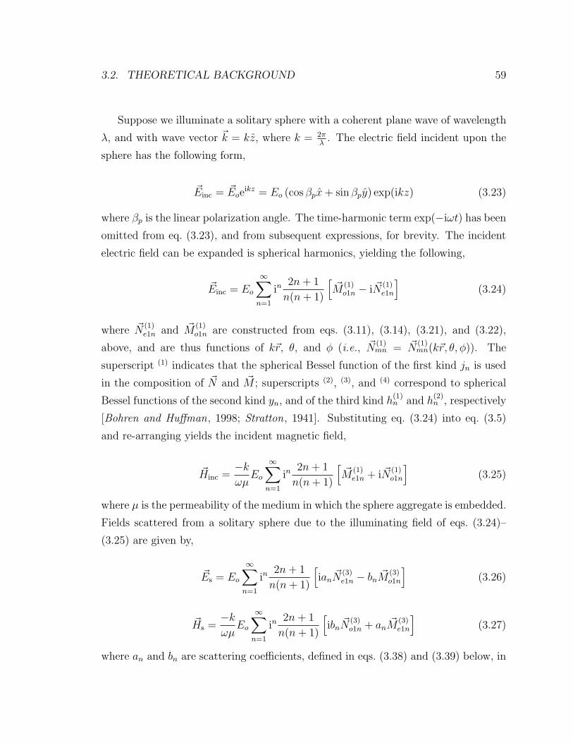
3.2. THEORETICAL BACKGROUND 59
Suppose we illuminate a solitary sphere with a coherent plane wave of wavelength
λ, and with wave vector k = kz, where k = 2πλ. The electric field incident upon the
sphere has the following form,
Einc = Eoeikz = Eo (cos βpx+ sin βpy) exp(ikz) (3.23)
where βp is the linear polarization angle. The time-harmonic term exp(−iωt) has been
omitted from eq. (3.23), and from subsequent expressions, for brevity. The incident
electric field can be expanded is spherical harmonics, yielding the following,
Einc = Eo
∞∑n=1
in2n+ 1
n(n+ 1)
[M
(1)o1n − i N
(1)e1n
](3.24)
where N(1)e1n and M
(1)o1n are constructed from eqs. (3.11), (3.14), (3.21), and (3.22),
above, and are thus functions of kr, θ, and φ (i.e., N(1)mn = N
(1)mn(kr, θ, φ)). The
superscript (1) indicates that the spherical Bessel function of the first kind jn is used
in the composition of N and M ; superscripts (2), (3), and (4) correspond to spherical
Bessel functions of the second kind yn, and of the third kind h(1)n and h
(2)n , respectively
[Bohren and Huffman, 1998; Stratton, 1941]. Substituting eq. (3.24) into eq. (3.5)
and re-arranging yields the incident magnetic field,
Hinc =−k
ωµEo
∞∑n=1
in2n+ 1
n(n+ 1)
[M
(1)e1n + i N
(1)o1n
](3.25)
where µ is the permeability of the medium in which the sphere aggregate is embedded.
Fields scattered from a solitary sphere due to the illuminating field of eqs. (3.24)–
(3.25) are given by,
Es = Eo
∞∑n=1
in2n+ 1
n(n+ 1)
[ian N
(3)e1n − bn M
(3)o1n
](3.26)
Hs =−k
ωµEo
∞∑n=1
in2n+ 1
n(n+ 1)
[ibn N
(3)o1n + an M
(3)e1n
](3.27)
where an and bn are scattering coefficients, defined in eqs. (3.38) and (3.39) below, in

60 CHAPTER 3. SCATTERING FROM RING PARTICLE CLUSTERS
the context of the multi-particle formulation of Mie theory. A detailed development
of eqs. (3.24)–(3.27) is found in Chapter 4 of Bohren and Huffman [1998].
3.2.2 Multi-Particle Scattering Using Mie Theory
Following Xu [Xu, 1995, 1997; Xu and Gustafson, 1997], suppose we define an ag-
gregate of L spherical scatterers, occupying some volume in ξηz-space as shown in
Figure 3.1. We illuminate this region with the coherent plane wave defined in eq.
(3.23). The electric and magnetic fields of the incident plane wave, Einc and Hinc, can
be expressed in a coordinate system that is centered on the jth sphere in the aggregate
by expanding the fields in vector spherical harmonics [Xu, 1995, 1997]. The develop-
ment is similar to the solitary sphere modeled in eqs. (3.24) and (3.25) above, except
that Xu uses a complex form to reduce eqs. (3.21) and (3.22) to a single equation,
ψmn(r, θ, φ) = Pmn (cos θ)zn(kr)e
imφ (3.28)
with 1 ≤ n ≤ ∞ and −n ≤ m ≤ n. This yields vectors Nmn and Mmn, which are
related to the even and odd forms described above by taking the real and imaginary
parts of the vector, respectively (e.g., Nemn = ReNmn
; Nemn = Im
Nmn
). Thus
in the multi-particle formulation, the incident fields are given by,
Einc(j) = −∞∑n=1
n∑m=−n
iEmn
[pjmn
N (1)mn + qjmn
M (1)mn
](3.29)
Hinc(j) = − k
ωµ
∞∑n=1
n∑m=−n
Emn
[qjmn
N (1)mn + pjmn
M (1)mn
](3.30)
where pjmn and qjmn are expansion coefficients of the original incident field in the jth
coordinate system. The term Emn is a field normalization factor, defined as,
Emn = Eoin(2n+ 1)
(n−m)!
(n+m)!(3.31)
Note that substitutingm = 1 and eq. (3.31) into eqs. (3.29) and (3.30) and simplifying
yields the incident field expansions for the solitary sphere formulation, eqs. (3.24) and

3.2. THEORETICAL BACKGROUND 61
(3.25).
Eqs. (3.29) and (3.30) are slightly modified forms of eq. (17) in Xu [1995]. The
single superscript in pjmn and qjmn is borrowed from Xu [1997] (Begin by comparing
eq. (30) from Xu [1995] with eq. (5) from Xu [1997], a later paper with notational
improvements).
The field incident upon the jth sphere in the aggregate is a superposition of the
original incident field and the fields that are scattered from all of the other spheres
in the aggregate,
Ei(j) = Einc(j) +∑l =j
Eljs (3.32)
Hi(j) = Hinc(j) +∑l =j
H ljs (3.33)
where Eljs and H lj
s denote the electric and magnetic scattered fields transformed from
the lth to the jth local coordinate system. For an individual sphere in the aggregate,
these scattered fields have the following form,
Es(j) =∞∑n=0
n∑m=−n
iEmn
[ajmn
N (3)mn + bjmn
M (3)mn
](3.34)
Hs(j) =k
ωµ
∞∑n=0
n∑m=−n
Emn
[bjmn
N (3)mn + ajmn
M (3)mn
](3.35)
Terms ajmn and bjmn are the scattering coefficients for the jth sphere in the aggregate,
and the superscript (3) of the vector spherical wave functions denotes the use of
spherical Bessel functions of the third kind (Hankel functions) in the field expansions
[Bohren and Huffman, 1998]. Xu [1997] shows that the scattering coefficients ajmn
and bjmn, which contain the effects of all multiple scattering behavior exhibited by the
aggregate, are determined by solution of the following linear system,
ajmn = ajn
⎡⎣pjmn −(1,L)∑l =j
∞∑ν=1
ν∑µ=−ν
(Alj
mnµνalµν +Blj
mnµνblµν
)⎤⎦ (3.36)

62 CHAPTER 3. SCATTERING FROM RING PARTICLE CLUSTERS
bjmn = bjn
⎡⎣qjmn −(1,L)∑l =j
∞∑ν=1
ν∑µ=−ν
(Blj
mnµνalµν + Alj
mnµνblµν
)⎤⎦ (3.37)
where ajn and bjn are the scattering coefficients of a single, isolated sphere, 1 ≤ (j, l) ≤L, and Alj
mnµν and Bljmnµν are vector translation coefficients which facilitate the trans-
lation of elementary spherical waves from the lth to the jth local coordinate system
(see Xu [1996] for a detailed discussion of these coefficients). The coefficients ajn and
bjn are computed directly from Mie theory (the well-known Mie coefficients),
ajn =mjψn(m
jxj)ψ′n(x
j)− ψn(xj)ψ′
n(mjxj)
mjψn(mjxj)ξ′n(xj)− ξn(xj)ψ′n(m
jxj)(3.38)
bjn =ψn(m
jxj)ψ′n(x
j)−mjψn(xj)ψ′
n(mjxj)
ψn(mjxj)ξ′n(xj)−mjξn(xj)ψ′n(m
jxj)(3.39)
where ψn and ξn are Ricatti-Bessel functions, and their primed counterparts denote
differentiation with respect to the argument of the function. We assume here that
the permeability of the spheres is identical to that of the surrounding medium. This
is not a necessary limitation [Bohren and Huffman, 1998], but it leads to the simpler
form of ajn and bjn presented in eqs. (3.38) and (3.39). At the risk of causing confusion,
the symbol commonly used to represent relative refractive index, m, has been used
in eqs. (3.38) and (3.39). It is defined as mj =√
εjεo, where εj and εo are the electric
permittivity of the jth sphere and of the surrounding medium, respectively. The
variable xj is the electrical size parameter of the jth sphere, defined as,
xj = (ka)j =2πaj
λ(3.40)
where aj is the radius of the jth sphere.
Eqs. (3.36) and (3.37) represent a system of 2LN(N +2) equations with an equal
number of unknown multiple scattering coefficients, where N is the highest order n
required for convergence of the expansion. Although this system could, in theory,
be solved by matrix inversion, this is often infeasible when the number of or size of
the spheres is large [Xu, 1995]. Fuller et al. [1986] employed an order-of-scattering
technique to solve for ajmn and bjmn. Xu employs an iterative method to find these

3.2. THEORETICAL BACKGROUND 63
coefficients.
In the far field, the total scattered fields from the aggregate of spheres can be
expressed as follows [Xu, 1997],
Es =L∑
j=1
exp(−ikδj) Es(j) (3.41)
Hs =L∑
j=1
exp(−ikδj) Hs(j) (3.42)
where δj = r · dj is the projection of the vector dj, pointing from the center of the
aggregate’s coordinate system to the center of the jth sphere, along unit vector r,
which points from the center of the aggregate’s coordinate system to an observation
point in the far field. Thus the term exp(−ikδj) is the phase shift, relative to the
coordinate system center, introduced by the positional offset of the jth sphere as
projected along the line-of-sight to the far field observer. Implicit in this formulation
is the limiting approximation that vectors between spheres comprising the aggregate
and an observer in the far field are parallel. Combining eqs. (3.41) and (3.42) with
eqs. (3.34) and (3.35) yields an expression for the far field scattering pattern of a
cluster of spheres,
Es =L∑
j=1
exp(−ikδj)N∑
n=1
n∑m=−n
iEmn
[ajmn
N (3)mn + bjmn
M (3)mn
](3.43)
Hs =k
ωµ
L∑j=1
exp(−ikδj)N∑
n=1
n∑m=−n
Emn
[bjmn
N (3)mn + ajmn
M (3)mn
](3.44)
Note the substitution of N for ∞ in the summation of n.
Far from the scatterers, one may describe the scattered field, and thus the scat-
tering properties of the aggregate by the scattering matrix formulation [van de Hulst ,
1981; Bohren and Huffman, 1998]:
[E‖sE⊥s
]=
exp(ik(r − z))
−ikr
[S2 S3
S4 S1
][E‖iE⊥i
](3.45)

64 CHAPTER 3. SCATTERING FROM RING PARTICLE CLUSTERS
where S1 through S4 are the scattering matrix elements for the aggregate, and the
subscripts ‖ and ⊥ indicate the components of the incident and scattered fields which
are parallel and perpendicular to the scattering plane, respectively. The scattering
plane is defined as the plane containing both the incident wave vector k and the
scattering direction r, which depends on θ and φ.
We limited our study to the scattering of like-polarized fields. That is, we com-
puted the parallel-polarized scattered field E‖s due to a parallel-polarized incident
field E‖i =∣∣∣ Ei
∣∣∣ (E⊥i = 0), and computed E⊥s due to a perpendicularly-polarized
incident field E⊥i =∣∣∣ Ei
∣∣∣ (E‖i = 0). Further limiting our far field observations to be
in cuts along the u-axis in Figure 3.1 (i.e. φ = 0), we see that E⊥i = 0 when Ei is
ξ-polarized, and E‖i = 0 when Ei is η-polarized. Referring to eq. (3.45), these two
polarizations are completely characterized by S2 and S1, respectively. The polarized
scattered intensity of the aggregate may now be summarily defined,
I11(θ) = |Sη1 (θ, φ = 0)|2 (3.46)
I22(θ) =∣∣∣Sξ
2(θ, φ = 0)∣∣∣2 (3.47)
where the superscripts ξ and η denote the incident E-field polarization. I11 and I22
are the polarized scattered intensity patterns of v-polarized scattered light given η-
polarized incident light, and u-polarized scattered light given ξ-polarized incident
light, respectively. Thus, I11 and I22 represent orthogonal polarization measurements
of the scattered signal along a u-axis cut in the uv-plane (see Figure 3.1).
3.2.3 Diffraction from an Amplitude Screen
We used the shadow projection technique outlined in Section 3.2 and shown in Figure
3.1 to generate an amplitude screen representative of the aggregate of spheres under
study. Diffraction is a coherence effect that is produced by a combination of the prop-
agation and interference of waves. Scalar diffraction theory applies—and produces
very accurate results—when the diffracting objects are large compared with the wave-
length (i.e. when the size parameter x is large), and when the diffraction pattern is
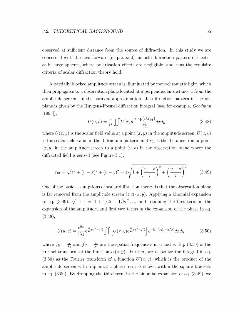
3.2. THEORETICAL BACKGROUND 65
observed at sufficient distance from the source of diffraction. In this study we are
concerned with the near-forward (or paraxial) far field diffraction pattern of electri-
cally large spheres, where polarization effects are negligible, and thus the requisite
criteria of scalar diffraction theory hold.
A partially blocked amplitude screen is illuminated by monochromatic light, which
then propagates to a observation plane located at a perpendicular distance z from the
amplitude screen. In the paraxial approximation, the diffraction pattern in the uv-
plane is given by the Huygens-Fresnel diffraction integral (see, for example, Goodman
[1995]),
U(u, v) =z
iλ
U(x, y)
exp(ikr01)
r201dxdy (3.48)
where U(x, y) is the scalar field value at a point (x, y) in the amplitude screen, U(u, v)
is the scalar field value in the diffraction pattern, and r01 is the distance from a point
(x, y) in the amplitude screen to a point (u, v) in the observation plane where the
diffracted field is sensed (see Figure 3.1),
r01 =√z2 + (u− x)2 + (v − y)2 = z
√1 +
(u− x
z
)2
+
(v − y
z
)2
(3.49)
One of the basic assumptions of scalar diffraction theory is that the observation plane
is far removed from the amplitude screen (z x, y). Applying a binomial expansion
to eq. (3.49),√1 + ε = 1 + 1/2ε − 1/8ε2 . . ., and retaining the first term in the
expansion of the amplitude, and first two terms in the expansion of the phase in eq.
(3.48),
U(u, v) =eikz
iλze
ik2z
(u2+v2) [
U(x, y)eik2z
(x2+y2)]e−i2π(xfU+yfV )dxdy (3.50)
where fU = uλz
and fV = vλz
are the spatial frequencies in u and v. Eq. (3.50) is the
Fresnel transform of the function U(x, y). Further, we recognize the integral in eq.
(3.50) as the Fourier transform of a function U ′(x, y), which is the product of the
amplitude screen with a quadratic phase term as shown within the square brackets
in eq. (3.50). By dropping the third term in the binomial expansion of eq. (3.49), we

66 CHAPTER 3. SCATTERING FROM RING PARTICLE CLUSTERS
have implicitly enforced the criterion that the phase contribution due to the 1/8ε2
term must be much less than a radian, or,
z3 π
4λ
[(u− x)2 + (v − y)2
]2max
(3.51)
This is the well-known criterion defining the Fresnel diffraction regime (e.g., Goodman
[1995]). If the phase introduced by the eik2z
(x2+y2) term in eq. (3.50) is also much less
than one radian,
z k(x2 + y2)max
2(3.52)
then eq. (3.50) simplifies further,
U(u, v) =eikz
iλze
ik2z
(u2+v2)
U(x, y)e−i2π(xfU+yfV )dxdy (3.53)
which is the Fourier transform of U(x, y). Eq. (3.53) is the Fraunhofer far field
approximation to the Huygens-Fresnel diffraction integral, and the criterion for its use
is given by eq. (3.52). The intensity measured in the far field (i.e., at the observation
plane a distance z from the amplitude screen) is equal to the magnitude of the field
squared,
I(u, v) = U(u, v)U∗(u, v) ∝ |F U(x, y)|2 (3.54)
where F is the Fourier transform operator. I(u, v) is proportional to the intensity of
the diffracted field.
3.2.4 Mie and Diffraction Theory: Some Practical Consider-
ations
Our code follows the formulation outlined in Section 3.2.2, making no other assump-
tions in its representation of the aggregate. The maximum number of expansion
terms N needed to assure convergence of the solution was determined algorithmically
according to the so-called Wiscombe stability criterion [Wiscombe, 1980], which for
8 < x < 4200 is given by N = xmax + 4.05x1/3max + 2, where xmax is the size parameter
of the largest sphere in the aggregate.

3.2. THEORETICAL BACKGROUND 67
The total memory requirement of the multiple scattering coefficients matrix is
on the order of M ∼ N4 + LN2, where L is the number of particles, and M is
in bytes. For large x, the computational cost of the Mie solution grows, roughly,
as x4 + Lx2 + 256x4/3. An important prerequisite step is to select an appropriate
minimum value of x—one which is sufficiently large to ensure that the spheres are in
the scalar diffraction theory regime, and yet sufficiently small so that Mie simulation
of aggregates computes in a reasonable time.
In adapting our diffraction theory approach to computer simulations, we require
some additional approximations beyond those introduced by the shadow projection
technique. In order to use a 2D Fast Fourier transform (FFT) to compute the diffrac-
tion pattern, we divided the amplitude screen into pixels of size ∆x by ∆y (we used
square pixels, ∆x = ∆y). Pixel size selection (i.e., choosing the spatial sampling
rate) is driven by three factors.
First, we need pixels that are small enough to well-represent the curved shadow
edges of a projected cluster of spheres. When viewing the amplitude screen as a
whole, the comprising particles should look like circles—not like blocks or staircases.
Second, we need pixels that are small enough to ensure that the main lobe of the
diffraction pattern is nearly free from the effects of aliasing. This is an important cri-
terion, since our investigation is focused on near-forward scattering. It is not possible
to completely eliminate aliasing, since the Fourier transform of the amplitude screen
is not band-limited (due to the finite extent of the shadow area and the discontinuity
present along its edge). We select the pixel size to ensure that the spatial sampling
frequency fs is large enough (fs =1∆x
= 1∆y
) to keep the effect of aliasing acceptably
small over the main lobe of the diffraction pattern. We set as a weaker criterion that
the first sidelobe is also as free as possible of aliasing effects.
Smaller pixels correspond to a higher sampling frequency fs, and therefore to a
lower frequency-domain resolution ∆f = fsK, for an FFT of fixed size K × K. The
third pixel size selection criterion is that the combined selection of K and ∆x, ∆y
must yield a resolution ∆f that is sufficient to reveal details in the diffraction pattern
that are necessary for comparison with the Mie results.
To summarize: For the Mie simulations, the size parameter must be large enough

68 CHAPTER 3. SCATTERING FROM RING PARTICLE CLUSTERS
to ensure that particles are within the scalar diffraction theory regime, but as small as
possible to minimize the computational cost. For the diffraction theory simulations,
we desire small pixels to minimize aliasing and to accurately represent the shape
of the particles, but large pixels for computational efficiency and frequency-domain
resolution. Selection of specific values for x, ∆x, and ∆y is discussed in Section 3.3.1.
Note that the Mie solution does not contain aliasing effects; its accuracy is limited,
however, by the number of expansion terms N used.
3.3 Simulation Results
We now compare Mie and diffraction theory predictions of the far field diffraction
pattern for several scenarios. The Mie calculations are performed using spheres of
relative refractive index m = 1.78 + i10−4. In the microwave frequency range, this
corresponds roughly to water ice at temperatures below −5o C [Sadiku, 1985]. We
study single-sphere, two- and three-sphere, and ten-sphere systems. We investigate
single sphere cases to: (1) select the pixel size of the amplitude screen; and (2) select
the minimum x required by this study. The two- and three-sphere simulations are
used to examine so-called pathological cases, i.e., cases where we expect discrepancies
between Mie and diffraction theory to be largest. The relative placement of spheres
in the simulation for the two- and three-sphere cases is determined using pre-defined
angles and distances as described in Section 3.3.2, and as shown in Figure 3.3. We
generate sphere locations for the ten-sphere cases randomly. Results for those simu-
lations are presented in Section 3.3.3.
Throughout this chapter, we compare the scattered signal intensity predicted by
Mie theory with diffraction theory for uz-plane cuts only (see Figure 3.1). This
approach simplified the execution of our simulations without loss of generality in
our comparison. We generated results for running hundreds of different aggregates,
all with unique orientations. The Mie theoretic polarization intensities given in eqs.
(3.46) and (3.47) are compared with diffraction theory results by taking a cut of
3.3. SIMULATION RESULTS 69
I(u, v), eq. (3.54), along the u-axis,
Iu(θn) = I(un, v = 0) (3.55)
where un denotes the value of u associated with the nth pixel along the u-axis from
the boresight (i.e., θ = u = 0) direction. For a diffraction pattern generated by
computing the K×K–point 2D–FFT of an amplitude screen, the angle θn is given by,
θn = arctan
(nλfsK
), 0 ≤ n ≤ K − 1 (3.56)
where n is the pixel number associated with un. For brevity, we drop the subscript
and refer to θn as θ from this point forward.
The two-sphere, three-sphere, and ten-sphere investigations summarized in this
chapter represent a total of 445 simulated cases. For the ith case of a given type (e.g.,
two-sphere, three-sphere, etc.), we define a difference measure ∆i between Mie and
diffraction theory,
∆i(θ) = I11(θ)− Iu(θ) (3.57)
where I11(θ) and Iu(θ) have been normalized by I11(0) and Iu(0), respectively. The
maximum difference for the ith case is defined as,
∆i,max = |∆i(0 ≤ θ ≤ θ1)|max (3.58)
where θ1 = arcsin(
3.822xmax
)is the first null in the diffraction pattern of single sphere
of size parameter xmax, corresponding to the largest sphere possible in the ith case
simulation. For the case where the incident radiation is natural light, the incident
energy is unpolarized—all polarizations are equally probable. The scattered field
intensity of natural light is determined from the sum I11(θ) + I22(θ). In the case of
coherent incident radiation, the near-forward diffracted signal is negligibly depolarized
and the scattered intensity has the same polarization as the incident intensity. Hence,
in eq. (3.57), it is sufficient to use either I11(θ) or I22(θ), as we have done.
For each type of case, we define an associated mean difference, ∆ and standard

70 CHAPTER 3. SCATTERING FROM RING PARTICLE CLUSTERS
deviation, σ∆,
∆(θ) =1
M
M∑i
∆i(θ) (3.59)
σ∆(θ) =
√√√√ 1
M
M∑i
(∆i(θ)−∆(θ)
)2(3.60)
where M is the total number of cases simulated of each type. The maximum mean
difference, ∆max, and maximum standard deviation, σ∆,max, on the interval 0 ≤ θ ≤ θ1
are defined in a manner analogous to eq. (3.58),
∆max =∣∣∆(0 ≤ θ ≤ θ1)
∣∣max
(3.61)
σ∆,max = |σ∆(0 ≤ θ ≤ θ1)|max (3.62)
Our angular range of interest is driven by our scientific application: the analysis
of radio waves forward-scattered from particles in Saturn’s rings during the Cassini
ring occultation experiment. In this case, detectable forward-scattered signals are
dominated by diffraction by individual ring particles over angles θ < θ1.
We discuss the use of these measures in the ensuing sections. Results of the
simulations are summarized in Tables 3.1–3.4 and Figures 3.4–3.8.
3.3.1 Scattering from a Single Sphere
The spatial sampling rate (discussed in Section 3.2.4) determines how coarsely or
finely the spheres’ shadows are discretized in the amplitude screen. Since the far field
diffraction pattern (eq. (3.53)) solution for a circular disc exists in closed-form—the
so-called Airy pattern, which is of the form A(θ) =[2J1(x sin(θ))
x sin(θ)
]2, with first null θ1
as defined in the text above—we determined the numerical diffraction pattern by
computing the Fourier transform of an amplitude screen representation of a circular
disc, and comparing it with the corresponding Airy pattern. We made this comparison
while varying the spatial sampling rate of the amplitude screen. Differences between
the FFT solution and the Airy pattern are introduced both due to aliasing, and due

3.3. SIMULATION RESULTS 71
to distortions caused by differences between the shape of a perfect circular disc and
its discretized counterpart. Based upon these simulations, we chose to use the spatial
sampling rate of ∆x = ∆y = rmin
12for all multi-particle simulations, where rmin is the
radius of the smallest sphere in the aggregate. With this sampling rate, the projected
area of a discretized sphere in our simulation was 97.5% of its true cross sectional
area (this percentage depends, to a small extent, on the method we used to generate
the amplitude screen shadow area within our code), and the effects of aliasing and
discretization were mitigated according to our stated criteria. This is seen clearly in
Figure 3.2(b)-(d), where the Airy pattern (dotted line) falls on top of the diffraction
pattern of the amplitude screen (dashed line) over the main diffraction lobe, as well
as the first sidelobe.
Since scalar diffraction theory is valid for large spheres only, and since the compu-
tational cost of solving the Mie solution grows very quickly with x and L as discussed
in Section 3.2.4, we seek to minimize x while retaining good agreement between Mie
and diffraction theory over the main lobe of the diffraction pattern. Figure 3.2(a)
summarizes the results. Here we show the difference between diffraction theory and
Mie theory, plotted in dB, for spheres of size parameter x = 20, 40, 80, and 140. We
normalize the abscissa scale by the value of the first null of a given particle’s diffrac-
tion pattern; each plot in the figure is scaled accordingly. Based upon these results,
and upon the time required to compute them, we determined that spheres of size
x = 40 were sufficiently large to show good agreement with diffraction theory over
the main lobe, while at the same time being computationally manageable. The agree-
ment between Airy, diffraction, and Mie solutions is shown in Figures 3.2(b)–3.2(d)
for x = 40, 80, and 140, respectively.
3.3.2 Scattering from Two and Three Spheres
Initially, we constructed sixty-three different configurations of two-particle aggregates,
and 176 different configurations of three-particle aggregates as a first foray into multi-
particle systems. For the two-particle systems, we varied the separation d between

72 CHAPTER 3. SCATTERING FROM RING PARTICLE CLUSTERS
0 0.1 0.2 0.3 0.4 0.5 0.6 0.7 0.8 0.9 1-50
-40
-30
-20
-10
0
10lo
g 10 M
ie -
DT
Difference between Mie and Diffraction Theory (DT) Results (Single Sphere)
x = 20x = 40x = 80x = 140
0 1 2-50
-40
-30
-20
-10
0
Nor
mal
ized
Inte
nsity
I/I o (
dB)
x = 40
0 1 2
x = 80
0 1 2
x = 140
AiryDiffractionMie
Normalized scattering angle θ/θ1(no units)
Normalized scattering angle θ/θ1
-50
-40
-30
-20
-10
0
-50
-40
-30
-20
-10
0
|
|
(a)
(b)
(c)
(d)
Figure 3.2: Comparison of Mie theory and diffraction theory solutions for scatteringof a linearly-polarized plane wave from a single sphere. (a) Difference between Mieand diffraction theory for size parameters ranging from 20 to 140. The data is plottedas a function of angle, normalized to the first null angle θ1 of the theoretical diffractionpattern of the given particle size x. (b)-(d) Comparison of Mie and diffraction theorywith the analytic (Airy) solution for the diffraction pattern of a circular disc, as xincreases from 40 to 140.

3.3. SIMULATION RESULTS 73
d
γ
x
z
IncidentPlane Wave
(a)
y
z
φγ
η
d2
d1
IncidentPlane Wave
(b)
Figure 3.3: Definition of geometry and parameters for simulation of the two- andthree-sphere cases. Distances d, d1, and d2 are measured from center-to-center.Spheres are of identical radius a, though differences have been introduced in (b)to provide 3D perspective.
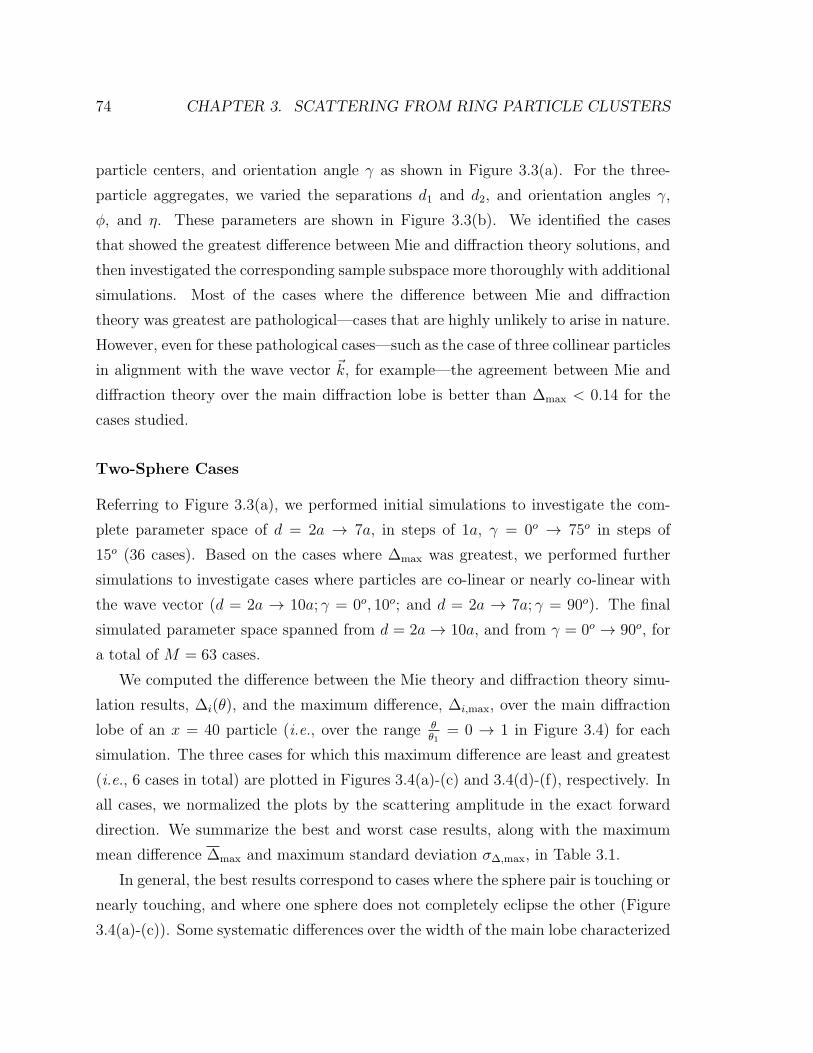
74 CHAPTER 3. SCATTERING FROM RING PARTICLE CLUSTERS
particle centers, and orientation angle γ as shown in Figure 3.3(a). For the three-
particle aggregates, we varied the separations d1 and d2, and orientation angles γ,
φ, and η. These parameters are shown in Figure 3.3(b). We identified the cases
that showed the greatest difference between Mie and diffraction theory solutions, and
then investigated the corresponding sample subspace more thoroughly with additional
simulations. Most of the cases where the difference between Mie and diffraction
theory was greatest are pathological—cases that are highly unlikely to arise in nature.
However, even for these pathological cases—such as the case of three collinear particles
in alignment with the wave vector k, for example—the agreement between Mie and
diffraction theory over the main diffraction lobe is better than ∆max < 0.14 for the
cases studied.
Two-Sphere Cases
Referring to Figure 3.3(a), we performed initial simulations to investigate the com-
plete parameter space of d = 2a → 7a, in steps of 1a, γ = 0o → 75o in steps of
15o (36 cases). Based on the cases where ∆max was greatest, we performed further
simulations to investigate cases where particles are co-linear or nearly co-linear with
the wave vector (d = 2a → 10a; γ = 0o, 10o; and d = 2a → 7a; γ = 90o). The final
simulated parameter space spanned from d = 2a → 10a, and from γ = 0o → 90o, for
a total of M = 63 cases.
We computed the difference between the Mie theory and diffraction theory simu-
lation results, ∆i(θ), and the maximum difference, ∆i,max, over the main diffraction
lobe of an x = 40 particle (i.e., over the range θθ1
= 0 → 1 in Figure 3.4) for each
simulation. The three cases for which this maximum difference are least and greatest
(i.e., 6 cases in total) are plotted in Figures 3.4(a)-(c) and 3.4(d)-(f), respectively. In
all cases, we normalized the plots by the scattering amplitude in the exact forward
direction. We summarize the best and worst case results, along with the maximum
mean difference ∆max and maximum standard deviation σ∆,max, in Table 3.1.
In general, the best results correspond to cases where the sphere pair is touching or
nearly touching, and where one sphere does not completely eclipse the other (Figure
3.4(a)-(c)). Some systematic differences over the width of the main lobe characterized

3.3. SIMULATION RESULTS 75
0 1 2
d = 2a, γ = 30o
0 1 2
d = 2a, γ = 15o
0 1 2
d = 3a, γ = 60o
0 1 2
Nor
mal
ized
Inte
nsity
I/I o
(dB
)
d = 10a, γ = 90o
0 1 2
d = 9a, γ = 90o
0 1 2
d = 8a, γ = 90o
AiryDiffractionMie
Nor
mal
ized
Inte
nsity
I/I o
(dB
)
-50
-40
-30
-20
-10
0
-50
-40
-30
-20
-10
0
-50
-40
-30
-20
-10
0
-50
-40
-30
-20
-10
0
-50
-40
-30
-20
-10
0
-50
-40
-30
-20
-10
0
Normalized scattering angle θ/θ1
Normalized scattering angle θ/θ1
(a)
(b)
(c)
(d) (e) (f)
Figure 3.4: Two spherical scatterers (x = 40): Comparison of results for the threebest cases ((a)-(c)) and three worst cases ((d)-(f)) of 63 simulated cases. Normalizingangle θ1 is the angle of the first null in the diffraction pattern of a single isolatedparticle. Parameters d and γ are defined in the text, and in Figure 3.3(a).

76 CHAPTER 3. SCATTERING FROM RING PARTICLE CLUSTERS
Table 3.1: Summary: Two-Sphere Scattering Investigations (x = 40). Parameters dand γ are explained in the text and in Figure 3.3(a). For the rows corresponding tospecific figures, ∆max = ∆i,max. For the row corresponding to the average of the 63cases, ∆max = ∆max. See Section 3.3 of the text for definitions of various ∆’s.
Case d γ ∆max σ∆,max
Fig. 3.4(a) 2a 30o .0040 –Fig. 3.4(b) 2a 15o .0061 –Fig. 3.4(c) 3a 60o .0102 –Fig. 3.4(d) 10a 90o .1458 –Fig. 3.4(e) 9a 90o .1375 –Fig. 3.4(f) 8a 90o .1237 –
Average (63 cases) – – .0151 .0457
cases where the spheres were further apart and one sphere completely eclipsed the
other, and thus the shadow projected onto the amplitude screen was that of a single
circular disc (Figure 3.4(d)-(f)). In those cases, as expected, the diffraction theory
solution closely matches the Airy pattern instead of the Mie solution. The best case
corresponds to d = 2a, γ = 30o; The worst case to d = 10a, γ = 90o.
Three-Sphere Cases
Figure 3.3(b) shows the geometry of our three-sphere simulations. The center-to-
center distances d1 and d2, and angles η, φ, and γ were used to completely parame-
terize the simulation space. We constructed the geometry from these parameters in
the following way: (1) We placed the spheres collinearly along the x-axis with one
sphere at the origin, and the other two at distances d1 and d2 on either side; (2) We
rotated the +x sphere about the z-axis to create the angle η between the 3 spheres;
(3) We rotated all three spheres about the z-axis to introduce the angle φ as shown;
(4) We rotated the three spheres about the y-axis by an angle γ as shown.
We simulated a total ofM = 172 cases during our investigation of the three-sphere
geometry. Initially, we explored the parameter space spanned by d1 = 2a, 4a; d2 =
3a, 5a; η = 45o, 90o, 135o, 180o; and φ, γ = 0o, 45o, 90o (144 cases). Based upon the
results of both these investigations and upon the results of our two-sphere simulations,
we extended the parameter space to include simulations of d1, d2 = 2a, 3a, 4a, 5a;

3.3. SIMULATION RESULTS 77
η = 180o; φ = 0; and γ = 70o, 80o (32 additional cases).
We summarize the results of the three-sphere simulations in Table 3.2. We discov-
ered that the poorest agreement, once again, correspond to the pathological case of
a co-llinear orientation of spheres whose shadows completely cover one another. The
separation distances d1 and d2 corresponding to the worst cases did not correspond to
the largest distances explored in the simulation space, in contrast to the correspond-
ing two-sphere investigations. The best-case results occurred for small separation
distances d1 and d2, and when there was minimal or no shadow overlap due to the
choice of η, φ, and γ. We present plots of the three best and three worst cases for the
three-sphere geometry in Figure 3.5.
Table 3.2: Summary: Three-Sphere Scattering Investigations (x = 40). Parametersd1, d2, η, φ, and γ are explained in the text and in Figure 3.3(b). For the rowscorresponding to specific figures, ∆max = ∆i,max. For the row corresponding to theaverage of the 176 cases, ∆max = ∆max. See Section 3.3 of the text for definitions ofvarious ∆’s.
Case d1 d2 η φ γ ∆max σ∆,max
Fig. 3.5(a) 2a 3a 45o 0o 45o .0032 –Fig. 3.5(b) 2a 3a 45o 0o 0o .0069 –Fig. 3.5(c) 2a 3a 45o 90o 0o .0077 –Fig. 3.5(d) 4a 3a 180o 0o 90o .1313 –Fig. 3.5(e) 4a 5a 180o 0o 90o .1262 –Fig. 3.5(f) 3a 3a 180o 0o 80o .1127 –
Average (176 cases) – – – – – .0183 .0304
3.3.3 Scattering from Ten Spheres
The geometry of a ten-sphere aggregate is loosely depicted in Figure 3.1. For each
case, we populated a volume of 18×18×12 units in ξηz-space with 10 spheres, where
x = 40 spheres had corresponding radii of a = 2 units. Sphere placement inside the
volume followed a uniform random distribution in space. Spheres were allowed to
touch each other, but sphere intersection within the volume was not allowed.

78 CHAPTER 3. SCATTERING FROM RING PARTICLE CLUSTERS
0 1 2
[d1 d
2 η φ γ] = [2a 3a 45o 0o 45o ]
0 1 2
[d1 d
2 η φ γ] = [2a 3a 45o 0o 0o ]
0 1 2
[d1 d
2 η φ γ] = [2a 3a 45o 90o 0o ]
0 1 2
[d1 d
2 η φ γ] = [4a 3a 180o 0o 90o ]
0 1 2
[d1 d
2 η φ γ] = [4a 5a 180o 0o 90o ]
0 1 2
[d1 d
2 η φ γ] = [3a 3a 180o 0o 80o ]
Nor
mal
ized
Inte
nsity
I/I o
(dB
)
AiryDiffractionMie
Nor
mal
ized
Inte
nsity
I/I o
(dB
)
-50
-40
-30
-20
-10
0
-50
-40
-30
-20
-10
0
-50
-40
-30
-20
-10
0
-50
-40
-30
-20
-10
0
-50
-40
-30
-20
-10
0
-50
-40
-30
-20
-10
0
Normalized scattering angle θ/θ1
Normalized scattering angle θ/θ1
(a)
(b)
(c)
(d) (e) (f)
Figure 3.5: Three spherical scatterers (x = 40): Comparison of results for the threebest cases ((a)-(c)) and three worst cases ((d)-(f)) of 176 simulated cases. Normalizingangle θ1 is the angle of the first null in the diffraction pattern of a single isolatedparticle. Parameters d1, d2, η, γ, and φ are defined in the text, and in Figure 3.3(b).

3.3. SIMULATION RESULTS 79
Monodistribution of Sphere Sizes
We simulated one hundred (M = 100) independent, randomly generated cases for the
ten-sphere monodistribution geometry. Each of these cases had ten x = 40 spheres
within the prescribed volume, giving a corresponding volume fraction for each case
of 0.086. Figure 3.6(a)-(c) shows the diffraction pattern of the three cases for which
∆i,max was least, and Figure 3.6(d)-(f) shows the diffraction pattern of the three cases
for which ∆i,max was greatest. We summarize the results in Table 3.3.
Figure 3.6(e) shows ∆i(θ) for all 100 cases, showing clearly how the differences
are distributed as a function of θ. The average ∆(θ) of the cases in Figure 3.6(e) is
shown in Figure 3.6(f). Figure 3.6(g) shows a plot of the standard deviation σ∆(θ).
The peak value in Figure 3.6(g) corresponds to σ∆,max, and is given in Table 3.3.
Table 3.3: Summary: Ten-Sphere Scattering Investigations (Monodistribution, x =40). Particle placement within the simulation space follows a uniform random spatialdistribution. For the rows corresponding to specific figures, ∆max = ∆i,max. For therow corresponding to the average of the 100 cases, ∆max = ∆max. See Section 3.3 ofthe text for definitions of various ∆’s.
Case ∆max σ∆,max
Fig. 3.6(a) .0029 –Fig. 3.6(b) .0029 –Fig. 3.6(c) .0030 –Fig. 3.6(d) .0544 –Fig. 3.6(e) .0438 –Fig. 3.6(f) .0388 –
Average (100 cases) .0024 .0186
To investigate the effect of dielectric loss, we simulated 70 additional 10-sphere
monodistribution cases. For each case, we varied the complex component of the
refractive index between m′′ = 0.1 and m′′ = 0. We found that the the effect of loss
on the simulated scattering behavior of the cluster was negligible. The results are
summarized in Figure 3.7.

80 CHAPTER 3. SCATTERING FROM RING PARTICLE CLUSTERS
0 1 2 0 1 2 0 1 2
0 1 2 0 1 2 0 1 2
0 1 2-0.06
-0.04
-0.02
0
0.02
0.04
0.06
0 1 2-2.5
-2
-1.5
-1
-0.5
0
0.5x10⁻³
0 1 2-40
-35
-30
-25
-20
-15
AiryDiffractionMie
-50
-40
-30
-20
-10
0
-50
-40
-30
-20
-10
0
-50
-40
-30
-20
-10
0
-50
-40
-30
-20
-10
0
-50
-40
-30
-20
-10
0
-50
-40
-30
-20
-10
0
Normalized scattering angle θ/θ1
Normalized scattering angle θ/θ1
Nor
mal
ized
Inte
nsity
I/I o
(dB
)N
orm
aliz
ed In
tens
ity I/
I o (
dB)
(a)
(b)
(c)
(d) (e) (f)
(g) (h) (i)
Normalized scattering angle θ/θ1
σ∆
(θ/θ
1) (
dB)
∆i(θ
/θ1)
∆i(θ
/θ1)
_
Figure 3.6: Ten identically-sized spherical scatterers (x = 40): Comparison of resultsfor the three best cases ((a)-(c)) and three worst cases ((d)-(f)) of 100 simulatedcases. Normalizing angle θ1 is the angle of the first null in the diffraction pattern of asingle isolated particle. Associated statistics: (g) superposed differences between Mieand Diffraction theory solutions for each simulated case, (h) average of differences inpanel (g), and (i) the corresponding standard deviation.
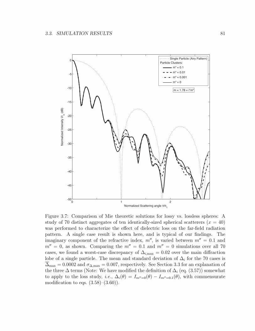
3.3. SIMULATION RESULTS 81
0 1 2-50
-45
-40
-35
-30
-25
-20
-15
-10
-5
0
Normalized Scattering angle θ/θ1
Nor
mal
ized
Inte
nsity
I/I o (
dB)
Single Particle (Airy Pattern)
m" = 0.1
m" = 0.01
m" = 0.001
m" = 0
m = 1.78 + i*m"
Particle Clusters:
Figure 3.7: Comparison of Mie theoretic solutions for lossy vs. lossless spheres: Astudy of 70 distinct aggregates of ten identically-sized spherical scatterers (x = 40)was performed to characterize the effect of dielectric loss on the far-field radiationpattern. A single case result is shown here, and is typical of our findings. Theimaginary component of the refractive index, m′′, is varied between m′′ = 0.1 andm′′ = 0, as shown. Comparing the m′′ = 0.1 and m′′ = 0 simulations over all 70cases, we found a worst-case discrepancy of ∆i,max = 0.02 over the main diffractionlobe of a single particle. The mean and standard deviation of ∆i for the 70 cases is∆max = 0.0002 and σ∆,max = 0.007, respectively. See Section 3.3 for an explanation ofthe three ∆ terms (Note: We have modified the definition of ∆i (eq. (3.57)) somewhatto apply to the loss study, i.e., ∆i(θ) = Im′′=0(θ) − Im′′=0.1(θ), with commensuratemodification to eqs. (3.58)–(3.60)).

82 CHAPTER 3. SCATTERING FROM RING PARTICLE CLUSTERS
0 1 2 0 1 2
0 1 2 0 1 2 0 1 2
0 1 2-0.1
-0.05
0
0.05
0.1
0.15
0 1 2-4
-3
-2
-1
0
1
2
0 1 2-35
-30
-25
-20
-15
-10
0 1 2
x10-3
-50
-40
-30
-20
-10
0
-50
-40
-30
-20
-10
0
-50
-40
-30
-20
-10
0
-50
-40
-30
-20
-10
0
-50
-40
-30
-20
-10
0
-50
-40
-30
-20
-10
0
Normalized scattering angle θ/θ1
Normalized scattering angle θ/θ1
Nor
mal
ized
Inte
nsity
I/I o
(dB
)N
orm
aliz
ed In
tens
ity I/
I o (
dB)
σ∆
(θ/θ
1) (
dB)
∆i(θ
/θ1)
Normalized scattering angle θ/θ1
AiryDiffractionMie
(a)
(b)
(c)
(d) (e) (f)
(g) (h) (i)
∆i(θ
/θ1)
_
Figure 3.8: Ten spherical scatterers. Particle sizes distributed uniformly betweensize parameters x = 40 and x = 80. Comparison of results for the three best cases((a)-(c)) and three worst cases ((d)-(f)) of 106 simulated cases. Normalizing angleθ1 is the angle of the first null in the diffraction pattern of a single isolated particle.Associated statistics: (g) superposed differences between Mie and Diffraction theorysolutions for each simulated case, (h) average of differences in panel (g), and (i) thecorresponding standard deviation.

3.4. DISCUSSION 83
Uniform Distribution of Sphere Sizes
We simulated one-hundred and six (M = 106) independent, randomly generated cases
with a uniform distribution in sphere size. The uniform size distribution ranged from
x = 40 to x = 80 (a = 1 → 2 units). Figure 3.8 shows the simulation results in an
analogous manner to the presentation of monodistribution results in Figure 3.6. Once
again, we find excellent agreement between Mie and diffraction theory predictions for
the far field scattering behavior of the aggregate, though the agreement is not quite
as good as it was for the ten-sphere monodistribution case (cf., Table 3.3 and Table
3.4).
Table 3.4: Summary: Ten-Sphere Scattering Investigations ( Uniform distribution,40 ≤ x ≤ 80). Particle placement within the simulation space follows a uniformrandom spatial distribution. For the rows corresponding to specific figures, ∆max =∆i,max. For the row corresponding to the average of the 106 cases, ∆max = ∆max. SeeSection 3.3 of the text for definitions of various ∆’s.
Case ∆max σ∆,max
Fig. 3.8(a) .0048 –Fig. 3.8(b) .0083 –Fig. 3.8(c) .0091 –Fig. 3.8(d) .1028 –Fig. 3.8(e) .0996 –Fig. 3.8(f) .0972 –
Average (106 cases) .0037 .0372
3.4 Discussion
In general, we observed excellent agreement between Mie and diffraction theory results
for the vast majority of cases simulated during this study. The two- and three-
sphere simulation sets contained geometric configurations of particles that produced
the worst-case agreement between Mie and diffraction theory. Invariably, the worst-
case results correspond to pathological cases where the particle alignment is co-linear
with k. A similar conclusion was reported by Marouf [1993]. Generally speaking,
∆i,max increases as the separation between particles in these co-linear pathological

84 CHAPTER 3. SCATTERING FROM RING PARTICLE CLUSTERS
x/a
y/a
-4 -2 0 2 4
-4
-2
0
2
4
(a)
-2 0 2
-2
0
2
θ/θ1
θ/θ
1
-2 0 2
-2
0
2
θ/θ1
θ/θ
1
(b) (c)
Figure 3.9: (a) An amplitude screen generated from a volume containing ten spheresand (b) its associated diffraction pattern. The scale of the amplitude screen is nor-malized by the sphere radius a. The diffraction pattern of an single, isolated particleis clearly seen in the diffraction pattern of the aggregate. Fine scale variation in thepattern intensity is due to the phase relationship of the individual particles, which iscontrolled by their relative spatial positions. Normalizing angle θ1 is the angle of thefirst null in the diffraction pattern of a single isolated particle. The case presentedin (a), (b) corresponds to Figure 3.6(a). The diffraction pattern of a single, isolatedparticle is shown in (c) for comparison.
3.4. DISCUSSION 85
cases increases (see Tables 3.1–3.2), over the range of separations addressed by our
study (up to 10a). Qualitatively speaking, when the k-aligned, co-linear particles are
separated by a few radii, the diffracted wave from the first particle begins to fill the
shadow region behind the first particle before it encounters the second particle, and
so on. Clearly, this endfire type of configuration is quite different from scattering
from a single sphere, but none of those differences, in terms of projected shadow area
on the amplitude screen, are captured by the diffraction theory model. By contrast,
when those scattered fields are not allowed to fill in behind the first particle before
encountering the second, etc. (i.e., when the particles are touching or very close
together), the scattered fields are more similar to those scattered by a single particle,
and thus more similar to the diffraction solution of a circular disc. This is true while
the particles are in each other’s near field, i.e., in the Fresnel region. Note that as the
particle separation is increased into the Fraunhofer region for the k-aligned, co-linear
particle case, we expect the agreement between Mie and diffraction theory to once
again improve. We have not attempted to identify the separation distance at which
∆i,max stops increasing.
For the ten-sphere simulations, monodistribution and uniform size distribution
simulations showed a factor of 15 to 20 difference between best- and worst-case ∆i,max.
As expected, ∆max was less than the best-case ∆i,max for both mono and uniform
distributions. We attribute this to the random nature of the spatial distribution,
which has a statistically equal likelihood of producing a positive or negative ∆i(θ) for
any given θ, and thus we expect ∆max to tend to zero as M → ∞.
As the number of particles in an aggregate grows, we expect the effect(s) of any
pathological behavior in the population to contribute only minimally to the overall
scattering behavior of the aggregate. For the vast majority of the particles in the
aggregate, the scattering behavior is well-characterized by diffraction theory, and
those behaviors effectively ‘wash out’ any pathological effects that may differentiate
the diffraction theory solution from the true EM scattering behavior. To be clear,
the underlying assumption here is that the vast majority of particles in the aggregate
are not co-linear and aligned with k, which is certainly the case in radio occultation
observations of Saturn’s rings.
86 CHAPTER 3. SCATTERING FROM RING PARTICLE CLUSTERS
Interestingly, we observe that the diffraction pattern of a cluster of particles com-
prises two main components: A component due to the scattering pattern of the
individual spheres in the aggregate, and a component representing the spatial ar-
rangement of the individual particles in the aggregate. This is akin to the so-called
element and array patterns in antenna theory, where the overall radiation pattern of
an antenna array is controlled by both the radiation pattern of the array’s individual
elements, and by the phase relationship between the elements, which is is controlled by
the position of the individual elements in space. This is evident in Figure 3.9, where
we show the diffraction pattern from an individual sphere alongside the diffraction
pattern of a particular ten-sphere aggregate. We discuss this phenomenon in more
detail in Section 4.2.
3.5 Amplitude Screen Model Results for Thick,
Homogeneous Rings
As discussed in Chapter 2, an interplay of gravitational and collisional forces at the
particle-to-particle level result in the formation of microstructure in Saturn’s rings,
on the scale of tens to hundreds of meters. Dynamical simulations of planetary ring
systems show that under most conditions, the steady-state distribution of particles
in Saturn’s rings is non-homogeneous (see Figure 2.11).
While a homogeneous model is unlikely to well-represent microstructure native
to Saturn’s main rings A–C (it is a model better suited to Ring D), it is useful for
two reasons. First, it provides a baseline case against which we observe degrees of
non-homogeneity in our measured experimental data; and second, it provides another
opportunity to test our amplitude screen method, since an analytic solution exists for
scattering from thick homogeneous rings.
EM forward-scattering from a homogeneous cloud of particles results in a broad-
ening of the forward scattering lobe, relative to the forward scattering lobe of a single
particle. Based on this, Marouf et al. [1982] worked out an exact analytical solution

3.5. AMPLITUDE SCREEN MODEL RESULTS FOR MPT RINGS 87
for the broadening due to scattering from a many particles thick (MPT), sparsely-
populated homogeneous ring model. We proceed by comparing the diffraction results
we computed using the amplitude screen method, with corresponding analytic solu-
tions for several instantiations of MPT homogeneous rings ranging in optical depth
between τ = 0.49 and τ = 8.24. Note that the use of the MPT model to estimate
particle size distributions in the rings is discussed in Section A.2 of Appendix A.
3.5.1 An Analytic Solution for Forward Scattering
Marouf et al. [1982] show that for a MPT ring model, the intensity of the forward-
diffraction lobe is given by,
I(τq, θ) = 2π
∫ ∞
0
ρJ0(2πρθ)e−τq(ew
˜Φ(ρ)τq − 1)dρ (3.63)
where θ is the boresight angle, ρ is the independent variable in the transform domain,
J0 is the zeroth-order Bessel function of the first kind, and τq is the oblique optical
depth as defined in eq. (1.1). w is the averaged single particle albedo, defined as,
w =Cs
Cs + Ca
(3.64)
where Cs and Ca are the average scattering and absorption cross-sections, respectively,
and the quantity Cs + Ca is often called the extinction cross section.
Noting that the Hankel transform (see Bracewell [2000], for example) is defined
as,
F (θ) = 2π
∫ ∞
0
f(ρ)J0(2πρθ)ρdρ (3.65)
we see that eq. (3.63) is the Hankel transform of the function f(ρ) = e−τq(ew˜Φ(ρ)τq−1).
Φ(ρ) is the Hankel transform of the normalized phase function of a single particle,
Φ(ρ) = 2π
∫ ∞
0
J0(2πρθ)
(Φ(θ)
4π
)θdθ (3.66)
where the single particle phase function is given by Φ(θ), and is equivalent to the

88 CHAPTER 3. SCATTERING FROM RING PARTICLE CLUSTERS
Fraunhofer diffraction pattern of the particle.
For the sake of simplicity, Marouf et al. [1982] develop their methods assuming a
Henyey-Greenstein model for Φ(θ),
Φ(θ) = Io(g)1− g2
(1− 2g cos θ + g2)3/2(3.67)
where g = 1 − 2/x is related to the electric size parameter x, previously defined in
eq. (3.40), Section 3.2.2. The factor Io(g) in eq. (3.67) is required to normalize the
integral of Φ to 4π over the half-space where Φ applies (see also eq. (3.66)),
∫ 2π
0
∫ π/2
0
Φ(θ) sin θ dθdφ = 4π (3.68)
Substituting eq. (3.67) into eq. (3.68) and evaluating yields the following normalizing
factor,
Io(g) =2g
1− g2
[1√
1− 2g + g2− 1√
1 + g2
]−1
(3.69)
For electrically large particles, g → 1 as x → ∞. Taking the limit of eq. (3.69) yields
limg→1 Io(g) = 1. For particles larger than x = 100 or so, Io = 1 is a reasonable
approximation.
The Henyey-Greenstein function is one of many possible model choices to represent
Φ(θ). For our purposes, we want to make a direct comparison between the predictions
of MPT theory and the results produced using the amplitude screen method. Thus
for our analysis, a more suitable phase function is the Airy scattering pattern of a
single sphere,
Φ(θ) = Io(x)
(2J1(x sin θ)
x sin θ
)2
(3.70)
which we have already shown to be well-approximated by our diffraction theory
method. As with the Henyey-Greenstein function above, the normalization factor
Io must be such that eq. (3.68) is satisfied. Substituting eq. (3.70) into eq. (3.68) and
solving for Io yields,

3.5. AMPLITUDE SCREEN MODEL RESULTS FOR MPT RINGS 89
Io(x) =x2
2
[1− J1(2x)
x
]−1
(3.71)
3.5.2 Comparison with the Amplitude Screen Model
Technically, the MPT theory of Marouf et al. [1982] requires that ring particles are
in each other’s far field. However the far field condition is not substantially violated
as long as the volume packing fraction of the rings,
fvol =Vparticles
Vslab
(3.72)
does not exceed 3% or so [Marouf , 2006–2010]. Here, Vslab is the volume of a slab of
the rings containing the particles that are projected to create the amplitude screen,
and Vparticles is the total volume of the ring particles contained within that slab.
We proceed by comparing forward scattering lobe predictions computed from the
theory of Marouf et al. [1982]; i.e., using eq. (3.63) with eqs. (3.66), (3.70), and (3.71);
with the results of amplitude screen diffraction simulations produced via the methods
described previously in this chapter. We construct and populate slab volumes in order
to obtain a desired oblique optical depth τq, iterating both the number of particles
in the model Np and the thickness of the rings Tr to ensure that the requirements
fvol ≤ 0.03, and Tr ≥ 30 are met. Tr is specified in units of particle diameters of the
largest particle in the model. According to Marouf, these are sufficient conditions for
the model to remain consistent with MPT theory. The oblique optical depth τq of
the amplitude screens is computed according to,
τq = −2 ln
(1− Ap
Atot
)(3.73)
where Ap is the shadow area of all particles projected onto the amplitude screen, and
Atot is the total area of the screen. Normal optical depth is related to the oblique
optical depth according to eq. (1.2). Eq. (3.73) derives directly from eq. (1.1), since
Io ∝ A2tot and I ∝ (Atot − Ap)
2. For our analysis (and without loss of generality),
we chose the ring opening angle B = 90o; thus τq = τ . Figure 3.10 shows examples

90 CHAPTER 3. SCATTERING FROM RING PARTICLE CLUSTERS
Next page.
Figure 3.10: Amplitude screen models of homogeneous, many particles thick (MPT)rings. The normal optical depth of the models ranges from τ = 0.49 to τ = 8.24.Higher optical depths were achieved by increasing the number of particles Np in thesimulation. The thickness of the rings Tr varies in each case, to ensure that thevolume fraction fvol of the rings does not exceed 3%. N simulations were performedfor each optical depth value studied, and their diffraction patterns averaged togetherto produce the solution. Panels (a)–(f) show single instantiations of the N amplitudescreens used to obtain the diffraction pattern averages shown in the correspondingpanels of Figure 3.11. Cases shown are as follows: (a) τ = 0.49; Tr = 32, Np = 1500,fvol = 0.001; (b) τ = 1.44; Tr = 32, Np = 3500, fvol = 0.014; (c) τ = 3.26; Tr = 43,Np = 9870, fvol = 0.029; (d) τ = 5.61; Tr = 73, Np = 17, 000, fvol = 0.03; (e)τ = 6.61; Tr = 86, Np = 20, 000, fvol = 0.03; (f) τ = 8.24; Tr = 107, Np = 25, 000,fvol = 0.03.

3.5. AMPLITUDE SCREEN MODEL RESULTS FOR MPT RINGS 91
x/a (no units)-60 -40 -20 0 20 40 60
y/a
(no
units
)
-60
-20
0
20
40
60
-40
-60
-20
0
20
40
60
-40
-60
-20
0
20
40
60
-40
-60 -40 -20 0 20 40 60
a b
c d
e f

92 CHAPTER 3. SCATTERING FROM RING PARTICLE CLUSTERS
Next page.
Figure 3.11: Comparison of the amplitude screen method with the theory of Maroufet al. [1982] for a homogeneous, many particles thick (MPT) model of the rings.Each diffraction solution shown in (a)–(f) is the computed average ofN unique diffrac-tion patterns, each derived from an amplitude screen that we generated using an MPTring model with identical parameters (Tr, Np, fvol). The parameters were selected toachieve a certain value of τ as indicated below; corresponding single instantiationsof these amplitude screens are shown in Figure 3.10(a)–(f). The Marouf et al. [1982]solution is generated using eqs. (3.63) and (3.70). The normal optical depths andnumber of unique averaged diffraction solutions N for each case are: (a) τ = 0.49,N = 40; (b) τ = 1.14, N = 40; (c) τ = 3.26, N = 50; (d) τ = 5.61, N = 40;(e) τ = 6.61, N = 40; (f) τ = 8.24, N = 55. All other relevant parameters are asindicated in Figure 3.10(a)–(f).
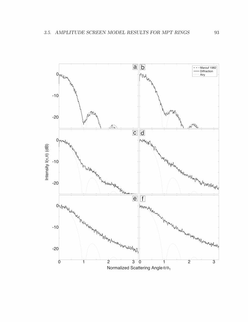
3.5. AMPLITUDE SCREEN MODEL RESULTS FOR MPT RINGS 93
0 1 2 3
-20
-10
0
0 1 2 3
Inte
nsity
I(τ,
θ)
(dB
)
Marouf 1982DiffractionAiry
Normalized Scattering Angle θ/θ1
-20
-10
0
-20
-10
0
a b
d
f
c
e
94 CHAPTER 3. SCATTERING FROM RING PARTICLE CLUSTERS
of amplitude screens having six different values of τ , ranging between τ = 0.49 and
τ = 8.24.
Eq. (3.63) gives the forward scattering lobe of the rings in a statistical sense. To
compare this result with our amplitude screen diffraction model, we must compute
the average diffraction pattern of N screens while holding Np and the slab volume
constant, thereby generating a statistical representation of scattering from rings of
a given packing fraction and optical depth. N must be large enough to average out
statistical fluctuations in the results—we determined that N ≥ 40 is sufficient in our
simulations. This topic is addressed in greater detail in Section 5.3.1.
Since the particle placement in each instantiation is unique, there is some variation
in the computed optical depth for each screen. For each of the N cases, the value of
τq is computed using eq. (3.73). The average value of τq of the N screens is used in
eq. (3.63) for the comparison. We used particles of electrical size x = 100 (see eq.
(3.40)) for all cases shown.
The results of the comparison are presented in Figure 3.11, showing excellent
agreement between the amplitude screen diffraction approach and the analytic ex-
pression for forward scattering, based upon the MPT model of the rings presented
in Marouf et al. [1982]. Similar good agreement between theoretical predictions and
numerical simulations of scalar diffraction by randomly blocked amplitude screen ring
models was reported by Marouf [1994, 1996]. The primary parameter of the thick
homogeneous rings model is the desired oblique optical depth τq; or alternatively, the
normal optical depth τ . The secondary parameters specifying the model are the thick-
ness of the rings Tr and the volume packing fraction fvol. If the homogeneous model
is to conform to the volume packing constraints of the MPT model, then fvol and
Tr are independent parameters only as long as the condition fvol ≤ 0.03 is satisfied.
For a given vignette size—i.e., the x- and y-dimensions of the amplitude screen (see
Figure 3.1)—and ring opening angle B, all other variables are specified automatically
for the model to remain self-consistent.

3.6. SUMMARY 95
3.6 Summary
A rigorous treatment of electromagnetic scattering from a cluster of spheres is afforded
by the application of the multiple particle formulation of Mie theory. However, to pro-
duce an accurate solution for scattering from electrically large spheres, and/or a large
number of spheres, the computational cost of this method is high. For our research
interest, scattering from clusters of electrically large Saturn ring particles in the range
x = 100 → 400, the computational requirement imposed by Wiscombe’s criterion and
the multi-particle formulation of Mie theory quickly exceeds the capability of today’s
computers—even for a small number (i.e., less than 50) of particles. By contrast,
the diffraction theory approach, initially developed by Marouf [1994, 1996, 1997] and
further developed here, captures the behavior of thousands of particles in small vi-
gnettes of Saturn’s rings, such as those produced by dynamical simulations [Salo,
1992; Schmidt et al., 2001; Salo et al., 2004; Morishima and Salo, 2006]. The method
is computationally limited only by the size of the 2D-FFT that must be performed
on the amplitude screen to generate the diffraction pattern.
By definition, diffraction theory does not account for the electromagnetic cou-
pling between ring particles that may be in each other’s near field—an effect which,
under some circumstances, could significantly alter the far field estimate. In this
chapter we have demonstrated that the far field radiation pattern produced by EM
scattering from aggregates of electrically large spherical dielectric particles is very
well-approximated by the results of scalar diffraction by their projected shadow area,
as long as the range of angular interest is limited to the near-forward direction.
Though the best results are seen for paraxial diffraction angles, diffraction theory
shows remarkable agreement with multi-particle Mie theory within the entire main
lobe of the particle cluster’s diffraction pattern.
We applied the amplitude screen method to MPT models of homogeneous rings,
for which an analytic description of the diffracted far-field exists. Results using the
diffraction theory method shows excellent agreement with corresponding analytic so-
lutions, providing a basis for further confidence in the amplitude screen approach.
The diffraction signature of anisotropic structure in Saturn’s rings is evident in

96 CHAPTER 3. SCATTERING FROM RING PARTICLE CLUSTERS
the Cassini radio occultation experimental data [Thomson et al., 2007]. As long as
this structure is not hidden by an unfortunate observational alignment with k, the
likelihood of which is diminished by the near-monolayer thickness of Saturn’s rings,
then the diffraction theory approach outlined in this chapter provides a powerful and
computationally efficient tool to quantitatively characterize, in a statistical sense,
near-forward scattering by particle distributions in Saturn’s rings.
The diffraction theory results contained in this chapter form the foundation for
the methods that we have developed to extract estimates of the physical dimensions
of ring microstructure from the radio occultation data. Those methods, which are the
subject of Chapter 5, combine the results of this chapter with key properties of the
signal that we receive from Cassini during radio occultation observations. In the next
chapter, we discuss the Cassini radio occultation experiment, and provide detailed
descriptions of the observation geometry, and of the properties of both transmitted
and received Cassini radio signals.
Chapter 4
The Cassini Radio Occultation
Experiment
In this chapter, we describe the key aspects of the Cassini radio occultation experi-
ment.
In Section 4.1 we discuss the properties of the transmitted and received signal, the
considerations necessary to optimize the spacecraft trajectory for the observations,
and present an overview of many of the physical ring properties that can be esti-
mated using radio occultation data. Additional details on these topics are provided
in Appendix A.
In Section 4.2 we discuss the specific properties of the received signal that indi-
cate the presence of ring microstructure, and explain some of the limiting aspects of
the measurement that affect our ability to estimate microstructure dimensions. We
present several examples of Cassini radio occultation data that contain evidence of
ring microstructure, that were discovered during post-processing of the Cassini ob-
servations. Section 4.2 serves as a prelude to Chapters 5 and 6, where we describe
methods to estimate microstructure dimensions from diffracted Cassini radio signals,
and report all ring locations where evidence of periodic microstructure (PM) is present
in the radio occultation data.
Eight of the first ten radio occultation observations of the Cassini mission occurred
during orbital flyby geometries that were optimized for the experiment. In Section
97

98 CHAPTER 4. THE CASSINI RADIO OCCULTATION EXPERIMENT
4.3, we discuss the details of this series of optimized observations, which were made
between May 3 and August 2 of 2005. Careful analysis of these observations led to
the uncovering of periodic microstructure in Rings A and B, along with estimates of
its physical dimensions.
4.1 Techniques, Observables, and Properties of the
Received Signal
The Cassini spacecraft and NASA’s Deep Space Network (DSN) together form an
instrument supporting radio occultation experiments to study Saturn’s rings. In
this dissertation, we describe several such occultation experiments using a radio link
between Cassini’s radio transmitter and at least one DSN receiver station. The radio
link is typically established at least 20 minutes before Cassini is due to pass behind
Saturn’s rings, as viewed from the DSN receiver(s). We calibrate the transmitted
signal during this time, before the signal begins to interact with the rings. As Cassini
continues on its trajectory in Saturn orbit, it moves behind the rings, as viewed from
the Earth. When this happens, the signal linking the transmitter and receiver is
said to be occulted (i.e., blocked) by the rings. The point where a ray linking the
transmitter and receiver intersects the rings is known as the ring piercing point (RPP).
The RPP traces out a trajectory in the ring plane that we refer to as the occultation
track. The experiment measures a one-dimensional sampling, along the occultation
track, of the transmission properties of the rings at radio wavelengths. The geometry
of a Saturn ring occultation experiment is shown in Figure 4.1. The occultation track
for the May 3, 2005 occultation of Saturn’s rings by Cassini is shown in Figure 4.2.
4.1.1 Transmitted and Received Signals
For Cassini, the transmitted signal is composed of three highly coherent, right hand
circularly polarized (RHCP) sinusoidal radio tones, well-separated in frequency, and
phase-locked to the same highly coherent local oscillator to ensure that any phase
modulation induced in the three transmitted tones by interaction with ring particles

4.1. PROPERTIES OF THE RECEIVED SIGNAL 99
To Earth
Antennafootprinton rings
Spacecraft
Rc
uE
ro
x y
z
x
y
uE
vs
r
uE
up
Figure 4.1: Ring Occultation Geometry. In the downlink configuration, a spacecrafttraveling at velocity vs points its antenna along the Earth intercept vector uE andtransmits a coherent, nearly monochromatic sinusoidal radio wave. The transmittingantenna illuminates a spot on the rings, the size of which has been greatly exaggeratedhere for clarity. Ring particles within the spot forward-scatter EM energy towardsEarth at a frequency that is determined by the geometry and relative motion as pereq. (4.1). The spectrum of color filling the spot in this figure is representative of theresulting Doppler contours on the rings. The vector r, which identifies a particularscattering region on the rings, has been drawn outside of the antenna spot—also inthe interest of clarity. The z-axis is the planet’s pole vector, which also defines thering plane orientation. The x-axis is the unit vector projection of uE into the ringplane, and y = z × x.
is accurately measured. Cassini uses an ultra-stable oscillator (USO) as its local
oscillator, with measured phase stability of σy = 2 × 10⁻¹³ over a 1-second interval,
where σy is the Allan deviation of the USO [Barnes et al., 1971; Kliore et al., 2004].
Cassini transmits at 13 cm, 3.6 cm, and 0.94 cm wavelengths, in the radio bands
known as S–, X–, and Ka–band, respectively. One may think of the transmitted

100 CHAPTER 4. THE CASSINI RADIO OCCULTATION EXPERIMENT
tones as separate radio channels at which the rings are probed. A consequence of
the high coherence of the transmitted signal is that radio wave diffraction, caused by
structures within the rings, is detectable. We discuss this in greater detail in Section
4.2.
Radio signals from Cassini are received in both left-hand and right-hand circular
polarizations, demodulated to an intermediate frequency (IF) band for sampling, and
recorded as complex samples of the signal voltage at the receiver output. The demod-
ulation frequency is controlled by a ‘predict’ file, which estimates the so-called sky
frequency—the transmitted frequency, Doppler-shifted by the motion of Cassini rel-
ative to the DSN receive antenna(s)—using predictive orbital mechanics algorithms
and the latest estimates of Cassini’s position and velocity. For the ring observa-
tions, the predict file is designed to continuously demodulate the sky frequency to 8
kHz, which is the center of a 16 kHz recording bandwidth, corresponding to 16,000
complex samples per second. The measured properties of the received signal are its
polarization, magnitude, and phase; and from these quantities as a function of time
we estimate its frequency, power, and power spectrum.
At each of the transmitted frequency channels (i.e., S-, X-, and Ka-bands), the
received signal comprises two components [Marouf et al., 1982; Tyler et al., 1983;
Marouf et al., 1983]:
1. Direct (Coherent) component: This is the transmitted sinusoid, attenuated and
phase shifted by the average effect of its interaction with the interceding ring
material along the very-near forward direction, well within the first several
Fresnel zones.
2. Scattered (Incoherent) component: This component of the signal corresponds
to energy forward-scattered towards the receiver from all of the ring parti-
cles illuminated by the transmitting antenna’s beam. The scattered signal is
incoherent—both due to the stochastic nature of the location of the scattering
ring particles, and due to the Doppler shift induced, relative to the transmit
frequency, by the relative motion of the transmitter, ring particles, and the re-
ceiver. With the best signal-to-noise ratio (SNR) available during both Cassini

4.1. PROPERTIES OF THE RECEIVED SIGNAL 101
and Voyager observations of Saturn’s rings, the observable bandwidth of the
scattered signal was approximately 4 kHz, centered (roughly) on that of the
coherent signal (see Figure 4.3).
Schematic illustration of the direct (coherent) and scattered (incoherent) signals, as
well as other key features of an example observed spectrum are presented in Figure
4.3.
4.1.2 Trajectory Design and Doppler Contours
Energy is forward-scattered from ring particles illuminated within the beam pattern
of the Cassini transmit antenna to the receiver on Earth at a particular Doppler
frequency fD relative to the Doppler-shifted transmit frequency,
fD =1
λ(vs − vp) · (up − uE) (4.1)
where fD is in Hz; λ is the wavelength of the transmitted sinusoid; vs and vp are
the Saturn-relative velocities of the spacecraft and the scattering ring particle, re-
spectively; up is the unit vector from the spacecraft to the scattering particle; and
uE is the unit vector from the scattering particle to the Earth, where the receiver is
located [Marouf et al., 1983]. Eq. (4.1) is a good approximation when the transmitter
(receiver) is much further away from the rings than the receiver (transmitter), so that
the unit vector from the transmitter (receiver) to receiver (transmitter) is essentially
equal to the unit vector from the scattering particle to the receiver (transmitter); see
Figure 4.1, and note that up is represented in the figure by a specific choice of u.
Energy that is forward-scattered towards Earth at a specific Doppler frequency
fD (see eq. (4.1)) maps to a locus of points in the ring plane. The Doppler con-
tours presented in Figure 4.2 show two instances during the May 3, 2005 occultation
of the Cassini spacecraft by Saturn’s rings. White lines represent 2 kHz intervals
in Doppler frequency; shading from blue through red represent the continuum of
positively- through negatively-shifted Doppler signals.
The occultation track geometry of the first several diametric Cassini ring occul-
tations were optimized by the Cassini tour designers to best align the contours of

102 CHAPTER 4. THE CASSINI RADIO OCCULTATION EXPERIMENT
Next page.
Figure 4.2: Occultation Geometry and Doppler Contours. Saturn is shown as it wasseen from Earth during Cassini’s REV 7 encounter on May 3, 2005. The green line isthe occultation track with ingress on the right and egress on the left, as the spacecrafttraveled from right to left in this view. Two Doppler contour maps are shown—oneeach for specific points during the ingress and egress observation. The antenna spotfor the Ka-band transmission are shown superimposed on the contours. The spotsize is smaller for the ingress observation because for this particular orbital pass, thespacecraft was closer to the rings during ingress. Bluer color represents a Dopplershift fD > 0; redder color corresponds to fD < 0. Doppler contours at 2-kHz intervalsare drawn in white. Contours of constant Saturn radius are shown in black, scaledrelative to the radial distance of the ring piercing point (RPP) at (x, y) = (0, 0).The REV 7 observation was optimized for alignment of radial and Doppler contours;however, some misalignment is unavoidable.

4.1. PROPERTIES OF THE RECEIVED SIGNAL 103
3dB Antenna Footprint (Ka-Band)
Y-Axis Location Relative to Radio Ray Piercing Point in Ring Plane (km)
REV 7 EGRESS DOPPLER CONTOURSignal Received at DSS 34 at 09:51:46 UTC May 3 2005
Radio Ray Pierces Ring Plane 136.4824×10³ km from Saturn Center
-600 -400 -200 0 200 400 600
-500
0
500
1000
X-A
xis
Pos
ition
Rel
ativ
e to
Rad
io R
ay P
ierc
ing
Poi
nt in
Rin
g P
lane
(km
)
-1000
0
0
+400 km
-400 km
REV 7 INGRESS DOPPLER CONTOURSignal Received at DSS 34 at 04:30:00 UTC May 3 2005
Radio Ray Pierces Ring Plane 128.729×10³ km from Saturn Center
Y-Axis Location Relative to Radio Ray Piercing Point in Ring Plane (km)
X-A
xis
Pos
ition
Rel
ativ
e to
Rad
io R
ay P
ierc
ing
Poi
nt in
Rin
g P
lane
(km
)
-600 -400 -200 0 200 400 600
-1000
-500
500
1000
0
0
0
104 CHAPTER 4. THE CASSINI RADIO OCCULTATION EXPERIMENT
constant Doppler frequency with the contours of constant radius, shown in black in
Figure 4.2. A close alignment of Doppler with radial location means that individual
ringlets/radial structures scatter energy at the same Doppler frequency. Ideally, this
leads to a received signal spectrum that maps energy at a given frequency to a specific
radial location on the rings. In practice, perfect alignment is extremely difficult if not
impossible to achieve, since it requires a very special spacecraft trajectory for each
occultation pass.
Because of orbital dynamics constraints, the achievability of good Doppler contour
alignment varies from pass to pass. From Figure 4.2, it is clear that the Cassini
REV 7 egress observation was better aligned than the REV 7 ingress observation.
Nonetheless, the ingress alignment is still reasonably good.
For optimized observations, the Doppler contour gradient within Cassini’s antenna
footprint on the rings is reasonably well aligned with the ring piercing point (RPP)
velocity vector vRPP—Doppler contours tend from low to high frequency across the
antenna footprint and in the direction of travel, as is evident in Figure 4.2. As
the leading edge of the Cassini high-gain antenna (HGA) pattern encounters a ring
feature, energy is scattered from the feature towards Earth at a (relatively) large
positive Doppler frequency. As the RPP passes through and past the feature, signals
scattered from the feature to Earth sweep from high to low in Doppler.
Since the induced Doppler shift is proportional to λ−1 (see eq. (4.1)), longer
(shorter) wavelengths yield Doppler contours that are proportionally expanded (con-
tracted) in the ring plane. The Doppler contour expansion (contraction) is matched
a commensurate increase (decrease) in the Cassini HGA beamwidth, which is propor-
tional to λ. Since vRPP is the same regardless of the transmit frequency, the net effect
is that the Doppler contours associated with longer wavelength transmissions transit
a feature more slowly, and thus the transition from low to high Doppler frequency
occurs over a broader range of radial locations of the RPP. Thus ring features that are
visible in spectrograms of the received signal appear slanted at an angle that scales
in direct proportion with with the transmitted signal wavelength. We illustrate this
point in Figure 4.4.

4.1. PROPERTIES OF THE RECEIVED SIGNAL 105
4.1.3 Observables
Despite the simplicity of the basic experiment, a surprising wealth of information
can be derived from the received signal. From the coherent component, we obtain
high-resolution diffraction corrected estimates of the optical depth of the rings for
each of the frequency channels along the occultation track trajectory [Marouf et al.,
1986, 2005a, b, 2006a, b, 2007b; Rappaport et al., 2008; Colwell et al., 2009; French
et al., 2010]. In turn, the optical depth profiles can be used to estimate accurately the
physical dimensions of density and bending waves (introduced in Chapter 2) which
exist throughout the rings [Rosen and Lissauer , 1988; McGhee et al., 2006; Rappaport
et al., 2006; Marouf et al., 2007a]. Estimates of the local ring thickness and surface
mass density follow directly from estimates of the physical dimensions of these waves
[Rosen, 1989]. For other resolved ring features, methods have been developed to
estimate particle sizes, ring thickness, and the degree of particle crowding [Marouf
et al., 1982, 1983; Zebker et al., 1983, 1985]. Optical depth profiles obtained from the
Voyager 1 radio occultation of Saturn resulted in the discovery of ten new waves in the
rings [Rosen and Lissauer , 1988; Rosen, 1989]. Eight of these waves were identified
as being caused by orbital resonances (introduced in Chapter 2) with specific moons;
the source of the other two remains a mystery.
Three techniques are used in concert to estimate ring particle size distributions
over the millimeter to several tens of meters size range [Marouf et al., 1982, 1983, 1986].
For small particles, combined measurements of the differential extinction and the sig-
nal phase at two or more frequencies are used to estimate the number density of ring
particles in the millimeter to decimeter size range. The diffraction lobes of particles
larger than the Cassini high-gain antenna (i.e., of radius a > 2 meters) are narrower
than the spacecraft antenna beamwidth; as a result, information regarding the num-
ber density of particles in that size range is contained in the scattered signal. Analysis
of the scattered signal yields number density estimates for particles ranging in size
between approximately 2 meters and several tens of meters; the upper size limit of the
estimate is controlled by the sampling interval of the measured diffraction pattern of
the rings. For particles in the intervening decimeter to 2 meter size range, a bistatic
scattering technique is used to sample the broader diffraction lobes of these particles.

106 CHAPTER 4. THE CASSINI RADIO OCCULTATION EXPERIMENT
In this case, the Cassini antenna is pointed away from the Earth by an angle that is
proportional to λ/2a for the smallest particle to be sensed in this size range.
The estimated particle size distributions can be used to compute the expected
optical depth at a given frequency, which can be checked against the measured optical
depth value as a method for determining the self-consistency of the model and for
characterizing the error in the estimate. A theoretical summary of techniques used
to produce estimates of these and other quantities is provided in Appendix A.
The high SNR of the Cassini occultation experiments relative to Voyager, com-
bined with the larger ring opening angles of 19.10−23.6o present during the Cassini’s
summer 2005 tour of Saturn, has resulted in the richest data set ever gathered with a
ring occultation experiment. High SNR is very helpful in these experiments, because
it improves our ability to probe the most optically thick regions of the rings (within
Ring B), and to detect weaker scattered and diffracted signals originating from within
the region of the rings that are illuminated by Cassini’s high-gain antenna.

4.1. PROPERTIES OF THE RECEIVED SIGNAL 107
Next page.
Figure 4.3: Ring Occultation Signal Properties. The coherent component of thereceived signal travels along the very-near-forward direction from the spacecraft toEarth (downlink configuration), with fD ≈ 0 due to the forward geometry (see eq.(4.1) with up = uE). The coherent signal is attenuated and phase shifted by its transitof the rings, relative to a coherent reference signal. The incoherent scattered signalis composed of energy scattered from particles along the near-forward direction, andspread in frequency according to eq. (4.1). The forward scattering lobes of particlesare drawn here as a spectrum of color to emphasize the geometric dependence offD. The power spectrum of actual Cassini data from a radial location of r ≈ 2.1Rs
(Ring A) is shown, color-coded to be self-consistent with the scattering depiction inthe figure, and with the Doppler contours of Figure 4.2. The non-Gaussian nature ofthe scattered signal indicates the presence of fine-scale structure in this region of therings.

108 CHAPTER 4. THE CASSINI RADIO OCCULTATION EXPERIMENT
Spacecraft
trajectory
-20
2
0 10 20 30
Frequency (kH
z)
Intensity (dB)
Rin
g D
epth
Co
heren
t Sign
al fro
m C
ASSIN
I
Rin
g M
aterial
CO
HEREN
TA
ND
SCATTERED
SIGN
AL
FOR
WA
RDSC
ATTERING
FROM
THE
RING
S
CA
SSINI-Earth
Line o
f Sigh
t
2A
2a
Co
heren
t Sign
al
θ4
The Scatterin
g A
ng
le Determ
ines th
e Streng
th
and
Frequ
ency o
f each Scattered
Sign
al Co
mp
on
ent
Beam
wid
th o
f Forw
ard Scattered
Sign
al is Inversely Pro
po
rtion
al to Particle Size
Scattering
Events w
ithin
the R
ing
s Occu
rat D
ifferent D
op
pler Lo
ci on
the R
ing
Plane
NA
SAD
eep Sp
ace Netw
ork
An
tenn
a
FFT
θ3
θ2
θ1
Scattered Sig
nal
Co
heren
t Sign
al
Scattered Sig
nal
θ5

4.1. PROPERTIES OF THE RECEIVED SIGNAL 109
Next page.
Figure 4.4: Doppler signature of a gap in the rings. Distinct features in Saturn’s ringsappear slanted in spectrograms of Cassini radio occultation data. The slant angledepends on the wavelength of the transmitted signal, as is evident by comparingthe X- and Ka-band spectrograms shown in panels D and E, respectively. PanelsA–C depict an ingress occultation sequence, and show portions of the X- and Ka-band antenna footprints on the rings (centered on P , the ring piercing point (RPP))moving with velocity vRPP as shown. In panels A–C, the values and relative scalingof the X- and Ka-band Doppler contours are represented by color within the antennafootprints as described in the caption of Figure 4.2. In panels D–E, color representsthe power contained in the scattered signal, as shown in the scale included to the rightof panel E. Points P1–P3 represent distinct locations |ro| of P during its motion alongthe occultation track (not shown). At P1 (panel A), the positively Doppler-shifted(i.e., blue-shifted) portion of both the Ka- and X-band footprints are illuminatingthe gap, which scatters no energy. Therefore only red-shifted Doppler signal energyis received when the RPP is located at P1. At P2, the X-band signal scatters largepositive and negative Doppler-valued signals from the leading and trailing gap edgesonly, with no scattering in-between. The Ka-band footprint is completely containedwithin the gap, scattering no energy. At P3, both footprints fully illuminate the rings,and broadband scattering is received at both wavelengths. Compare panels A–C andtheir descriptions with the scattered spectrum at points P1–P3 in panels D and E.

110 CHAPTER 4. THE CASSINI RADIO OCCULTATION EXPERIMENT
134133.6
133.2133.8
133.2
Saturnocentric D
istance (Thousands of km
)
Rings
133.8133.4
133
Rings
GapP
1P
2P
3
Ka-B
andF
ootprint X
-Band
Footprint
133133.2
133.4133.6
133.8134
0
Frequency (Hz)-1000
-500
500
1000
P1
P2
P3
133133.2
133.4133.6
133.8134
P1
P2
P3
Ka-B
and Spectrogram
X-B
and Spectrogram
vR
PP
AB
C
DE
0 5 10 15 20
dB Relative to Noise Floor
Negative D
opplerP
ositive Doppler

4.2. DETECTION OF MICROSTRUCTURE IN THE RINGS 111
4.2 Detection of Microstructure in the Rings
Cassini radio signals at S-, X-, and Ka-bands (13-, 3.6-, and 0.94-cm λ) are generated
from a single ultra-stable oscillator (USO), as described in Section 4.1. A consequence
of the high coherence of the transmitted signal is that radio wave diffraction, caused
by structures within the rings, is detectable. Diffracted signals originating from ring
microstructure and macrostructure (see Chapter 2) contribute to the shape and fea-
tures of the frequency spectrum of the received signal. Radio waves diffracted from
large-scale structures such as ring divisions and gaps—with length scales on the order
of tens to thousands of kilometers—modulate the amplitude of the coherent compo-
nent of the received signal. This was first observed and reported during the Voyager
radio occultation experiment; see Marouf and Tyler [1982] for an excellent example
of microwave edge diffraction from the Encke gap.
The high-resolution optical depth profiles mentioned in Section 4.1 are obtained
by removing the effects of diffraction from the received coherent signal, producing
sharpened optical depth profiles that are not diffraction-limited (e.g., Marouf et al.
[1986]; Rosen [1989]). This process is described in detail in Appendix A. In this case,
diffraction is an unwanted artifact that corrupts the measured direct signal, degrading
the resolution of the profiles to scales larger than several Fresnel scales of diffraction.
4.2.1 Diffraction from Ring Microstructure
Diffraction effects are processed out of received Cassini signals to sharpen optical
depth profiles of the rings. But diffraction is not always an unwanted signal artifact
of the measurement technique—in our analysis, we use diffracted signals to detect
and estimate the dimensions of ring microstructure.
Where microstructure exists within the rings, the local optical depth may vary
significantly over short distances. As the Cassini radio signal probes the rings along
the occultation track, these variations modulate the amplitude of the coherent signal
with much greater frequency than the modulation induced by macrostructure. For
structures on the order of tens to hundreds of meters, the corresponding optical depth
variation is well-sampled by the experiment (the 16-kHz sample rate corresponds to

112 CHAPTER 4. THE CASSINI RADIO OCCULTATION EXPERIMENT
one sample every 1–2 meters of RPP movement along the occultation track; see vRPP
in Table 4.1). In the special case of periodic microstructure, the induced amplitude
modulation is also periodic, and the frequency spectrum of the received signal (at
S-, X-, and Ka-bands) contains sidelobes similar to those characteristic of an AM
radio signal. A complementary point of view is that periodic microstructure in the
rings behaves like a diffraction grating (to first order), producing detectible first-order
diffraction (grating) lobes when illuminated by the highly coherent transmitted signal
from Cassini.
The diffraction signature of individual particles and of their arrangement in an ag-
gregate is contained in the overall diffraction pattern of ring microstructure, as shown
in Chapter 3. The scattering behavior of microstructure is analogous to the far-field
radiation pattern of a multi-element antenna, which is computed from the far-field
pattern of the comprising antenna elements in combination with the phase relation-
ships between those elements—the so-called element and array factors mentioned in
Section 3.4.
In a ring occultation experiment, the physical dimensions of ring microstructure
are inferred from its diffraction signature in a statistical sense only for two main
reasons. First, ring particles are moving at speeds ranging between approximately 16
and 24 km/s in their Keplerian orbits about Saturn, within the main rings. We sample
the radio signals at 16 kHz and Fourier transform blocks of 4096 complex samples;
thus one spectral frame of processed data corresponds to approximately 1/4-second of
observation time. Ring particles move approximately 4–6 km along their orbits during
this period, and the RPP moves between 5–6 km along the occultation track. This
motion effectively averages the diffraction signature of any microstructure comprising
particles imaged during a given spectral frame. We could reduce the integration time
in an effort to minimize this effect, but the improvement is not beneficial (particles
move several meters during a single sample) and doing so degrades the SNR of the
spectral frame. And second, the microstructure itself (to varying degrees that depend
on the strength of and type of microstructure) is constantly being destroyed and re-
formed within the rings, as mentioned in Section 2.2.
Nonetheless, we expect estimates of ring microstructure dimensions that derive

4.2. DETECTION OF MICROSTRUCTURE IN THE RINGS 113
from its diffraction signature to be accurate measures of the local averages of those
dimensions. The reason for this is that locally, the statistics of ring microstructure are
controlled by properties such as particle size distribution, volume and surface mass
density, local gravitational influences, etc., which do not change significantly on the
spatial scale of the 4–6 km sample averaging (in most regions of the rings), or on the
temporal scale of the Cassini mission’s lifetime.
4.2.2 Evidence of Ring Microstructure
Examples of diffraction from ring microstructure are shown in Figure 4.5. Panels
A and B show spectrograms of the received signal, produced from X-band data
received during our May 3, 2005 ring occultation experiment. Periodic microstructure
is evident here (see figure caption), within the regions bounded by dashed lines (i.e.,
within the regions 123.15–123.3 and 123.7–124.4 thousand km from Saturn’s center).
We average these regions to produce the spectra shown in panels C and D.
In panel C, sharp sidelobes at ±70–100 Hz relative to the strong (∼35 dBn, or
decibels relative to the sensible noise floor) coherent signal are clearly seen. These
sidelobes are characteristic of diffraction from regions of periodic optical depth within
the rings; they represent the first-order diffraction lobes of periodic microstructure.
The coherent carrier and sidelobes are superimposed on a broader scattered signal,
which peaks at ∼10–12 dBn in the center of the panel and appears consistent with
homogeneously-distributed rings or possibly a packed monolayer structure; cf. Figures
3.11 and 5.10.
Panel D also contains evidence of PM, although the sidelobe peaks are not as
prominent as in Panel C. In this case, the background scattered signal shows an
asymmetry characterized by a near-linear decrease in the scattered signal power over
the interval -500 to 500 Hz. This is caused by averaging the scattered signal over a
range that includes an absence of positive Doppler scattering—see the portion of the
averaged region that is close to 123.7×10³ km in panel A.
We averaged the spectrogram in Panel B to produce the spectrum shown in Panel
E. Here, we also see evidence of microstructure. Though more subtle than indications

114 CHAPTER 4. THE CASSINI RADIO OCCULTATION EXPERIMENT
of PM, the double humps on either side of the coherent signal may possibly indicate
the presence of gravitational wakes, which are known to exist broadly throughout
Rings A and B [French et al., 2007]. Compared with Panel C, the humps in Panel E
show an enhancement in the scattered power in the range -500–500 Hz, where the peak
signal level of the humps is ∼15 dBn, compared with ∼10–12 dBn seen in Panel C. In
Chapter 5, we show that simulated RF signals forward-scattered from gravitational
wakes produce similar enhancements in near-forward scattering, reminiscent of the
humps shown in Panel E; see Figure 5.10.
PM features evident in our spectrograms show an obvious slanting that depends
on the transmitted signal wavelength, similar to the feature slanting discussed in
Section 4.1.2 and illustrated in Figure 4.4. There is no high-to-low frequency sweeping
associated with diffraction from ring microstructure—the Doppler frequency of the
first-order diffraction sidelobes is controlled by the physical dimensions of the PM.
The slanting of the feature is evident in the different radial locations that mark the
beginning (and end) of the positive and negative Doppler sidelobes diffracted by the
PM feature.
For PM features in the rings, the measured Doppler frequency of the sidelobes
is the same at all three Cassini transmit wavelengths. This is because the sidelobe
diffraction angle θd (discussed in greater detail in Section 5.2) and the spacing of
Doppler frequency contours (discussed in Section 4.1.2) in the ring plane are both
proportional to λ, compensating for each other exactly. The slanting and Doppler
properties of signals diffracted from PM are explained illustratively in Figure 4.6. We
explain the properties of PM diffraction more thoroughly in Section 5.2.

4.2. DETECTION OF MICROSTRUCTURE IN THE RINGS 115
Next page.
Figure 4.5: Diffraction from ring microstructure. Panels A and B show spectro-grams of X-band (3.6-cm λ) received during REV 7 ingress Cassini radio occultationobservations. The coherent signal is the horizontal red line near the center of thespectrograms. In A, the diffraction signature of microstructure appears as roughlyparallel lines displaced ±70–100 Hz from the coherent signal. Three sets of dashedlines and indicated ranges in A and B identify the swaths averaged to form thespectral plots shown in C–E, as shown. Spectrograms of REV 12 ingress data (notshown) were also averaged and are plotted in C–E. REV 7 occultation data produceda stronger scattered signal than REV 12 data because Cassini was ≈70,000 km closerto the rings during REV 7 (see Fig. 4.9). In C, we see the sharp first-order diffractionlobes characteristic of periodic microstructure (PM). The PM signal is superimposedon background scattering that appears fairly homogeneous. PM is also evident inD, but the sloped background scattering shelf indicates that the PM is superposedon an unknown anisotropic background structure. The soft double lobes in E arecharacteristic of scattering from crowded monolayers, but it is unknown if that isuniquely true or if gravitational wakes or other anisotropy in the rings could producethis spectrum. The magnitude of the coherent signals in C–E vary inversely withaverage optical depth τ over the region (τ ≈ 1.1 in panels C–D; τ ≈ 0.8 in panel E).In all panels, signal power is plotted in decibels relative to the sensible noise floor,abbreviated dBn.

116 CHAPTER 4. THE CASSINI RADIO OCCULTATION EXPERIMENT
(d) (e)
-1 0 15
10
15
20
25
30
35
40
Sig
nal P
ower
(dB
n)
-1 0 1Frequency (kHz)
-1 0 1
Fre
quen
cy (
kHz)
-1
-0.5
0
0.5
1
Radial Distance from Saturn (Thousands of km)123 123.5 124 126.5 127 127.5124.5 126
C
Coherent Signal
126.0-127.5123.7-124.5123.15-123.3
ED
dB R
elative to Noise
0
5
10
15
20
REV 7 REV 12
BA

4.2. DETECTION OF MICROSTRUCTURE IN THE RINGS 117
Next page.
Figure 4.6: Doppler signature of periodic microstructure in the rings. Panels A–Cdepict an ingress occultation sequence, showing a portion of the Cassini high-gainantenna (HGA) footprint transiting the rings from right to left with velocity vRPP.The rings piercing point (RPP) is shown at three distinct locations P1–P3 during thepanel sequence. A small blue (red) dot represents the origin within the HGA beamof the positive (negative) Doppler-shifted first-order diffraction lobes of the PM atX-band. At these locations, Cassini signals are diffracted through an angle θd towardsEarth; see Section 5.2 for a more thorough explanation. Similarly, a large blue (red)dot represents the origin of S-band sidelobe diffraction within the HGA footprint. X-and S-band signals originate in different locations because θd is proportional to λ;Doppler frequencies are the same at all transmitted λ because the Doppler contourspacing in the ring plane is proportional to λ in a way that exactly compensates fordifferences in θd at different transmit wavelengths. The slanting of PM features in thespectrograms is proportional to the distance between the diffraction lobes (i.e., thered/blue dots) at each transmitted λ—thus spectrograms of the S-band data appearmore slanted than X-band, which appear more slanted than Ka-band. Comparepanels A– C and their descriptions with the scattered spectra at points P1–P3 inpanels D and E. See Figure 6.3 for a comparison of PM diffraction at 13-, 3.6-, and0.94-cm wavelengths.

118 CHAPTER 4. THE CASSINI RADIO OCCULTATION EXPERIMENT
Saturnocentric D
istance (Thousands of km
)
X-B
and Spectrogram
S-B
and Spectrogram
DE
Frequency (Hz)
122.8123
123.2123.4
123.6
-500 0
500
P1
P2
P3
122.8123
123.2123.4
123.6
P1
P2
P3
123123.2
123.4123.6
123123.2
123.4122.8
123123.2
123.4
P1
P2
P3
Periodic Microstructure
Rings
Rings
X-B
andD
iffractionLobes
S-B
andD
iffractionLobes
vR
PP
AB
C
DE
0 5 10 15 20
dB Relative to Noise Floor

4.3. CASSINI RING OCCULTATION OBSERVATIONS, MAY–AUGUST 2005119
4.3 Cassini Ring Occultation Observations, May–
August 2005
The Cassini spacecraft flew 4 orbits of Saturn between May 3 and August 2 of 2005
that were optimized to align Doppler contours with radial contours, as described in
Section 4.1. These four orbits, named REV 7, 8, 10, and 12 according to a NASA/JPL
Cassini Tour convention, produced data for both ingress and egress observations on
each orbital flyby, generating eight radio occultation data sets at each of the three
transmit frequencies (13 cm, 3.6 cm, and 0.94 cm wavelength) for a total of 24 data
sets.
90o
N
Goldstone DSN
Madrid DSN
Canberra DSN
180o
W 135o
W 90o
W 45o
W135o
E
90o
S
45o
E0o
90o
E
0o
Figure 4.7: Location of DSN complexes around the world.
As mentioned in Section 4.1, NASA’s Deep Space Network (DSN) is an integral
component in the ring occultation experiment. There are three primary DSN facilities:
Goldstone (35o 25.529′ North, 116o 53.383′ West), Madrid (40o 25.738′ North, 4o
14.963′ West), and Canberra (35o 24.160′ South, 148o 58.878′ East), each separated
from the other by approximately 120o of longitude (see Figure 4.7) in order to provide
near-constant coverage to any spacecraft mission served by the DSN. The choice of

120 CHAPTER 4. THE CASSINI RADIO OCCULTATION EXPERIMENT
DSN location and receiver was dictated by the frequency coverage required by the
experiment, and by the visibility of Cassini at the three DSN sites during Earth receive
time (ERT) of Cassini’s signal. Generally, this is determined by the elevation angle of
Cassini above the local horizon; see Appendix B. Cassini signals are received at the
DSN ground stations approximately 80–90 minutes after their transmission, delayed
by the one-way light time from Cassini to the Earth present during the summer of
2005.
The local ring longitude and Cassini-RPP distance of the REV 7, 8, 10, and 12
observations are shown in Figures 4.8 and 4.9, respectively. For our purposes, zero
local ring longitude is defined by the projection in the ring plane of the unit vector
pointing from Saturn to the Earth at the time of the observation.
4.3.1 Details of the REV 7–12 Observations
The predicted timing, geometry, and operational details of the REV 7, 8, 10, and 12
observations are summarized in Figures 4.10–4.13 [Marouf , 2006–2010]. The start and
end Earth receive times of the live movable block (LMB) are given in coordinated
universal time (UTC) in the upper right and left of the figures (Figure 4.10 gives
times in pacific time (PT) as well). The LMB is a planned sequence of operations
that must be performed during the observation, which is uploaded as a single block to
the spacecraft to command its onboard equipment. Event times within an LMB are
relative to an epoch that can be updated a week to ten days before a given experiment,
based on an accurate spacecraft trajectory prediction.
The orientation of Saturn as seen from the Earth is shown in the center of Figures
4.10–4.13. The occultation track is shown as a black line with ticks marking 10
minute intervals in time during Cassini’s orbital pass; the A, B, C, and F rings are
also labeled. In the lower half of Figure 4.10, the start and end times of ring (ROI,
ROE) and Saturn (SOI, SOE) occultation ingress and egress events are noted in both
UTC and PT. The predicted beginning and end times of geometric occultation ingress
and egress are also noted. In Figures 4.11–4.13, ROC and SOC are used instead to
denote blocks of time corresponding to ring and Saturn occultations, respectively.

4.3. CASSINI RING OCCULTATION OBSERVATIONS 121
Next page.
Figure 4.8: Occultation track longitudes during the REV 7, 8, 10, and 12 ring oc-cultation observations, May–August 2005. The upper graphic shows the occultationtracks as seen from above Saturn’s north pole. For our purposes, zero longitude isdefined as the projection in the ring plane of the vector from Saturn to Earth at thetime of the observation. In the lower panels, the ingress and egress occultation lon-gitudes are plotted separately and in greater detail. Rings A–D are shown as shadedbands in the upper panel (all unlabeled), and also in the lower panels where onlyRing D is unlabeled, for brevity.

122 CHAPTER 4. THE CASSINI RADIO OCCULTATION EXPERIMENT
150o
30o
210o
60o
240o
90o270o
120o
300o
330o
180
0o
100000 km
Saturn(Top View)
Saturnocentric Distance (Thousands of km)80 100 120
65
70
75
80
85
90
95
100
105Lo
ngitu
de o
f RP
P (
degr
ees)
Ring A Ring B Ring C
80100120
246
248
250
252
254
256
258
260
262
Long
itude
of R
PP
(de
gree
s)
Ring A Ring C Ring B
REV 7
REV 10 REV 12
REV 8
To EarthINGRESSEGRESS
IngressTracks
EgressTracks
180o
Ring
Longitude

4.3. CASSINI RING OCCULTATION OBSERVATIONS 123
Cas
sini
to R
PP
Dis
tanc
e (T
hous
ands
of k
m)
80 100 120 140
200
250
300
350
Saturnocentric Distance (Thousands of km)
80100120140
200
250
300
350
EGRESS INGRESS
Cas
sini
to R
PP
Dis
tanc
e (T
hous
ands
of k
m)
Sat
urn
Occ
ulta
tion
Reg
ion
REV 7
REV 10 REV 12
REV 8
Figure 4.9: Distance from Cassini to the ring piercing point (RPP) during the REV7, 8, 10, and 12 observations. Ingress and egress are shown separately, with a brokenregion in-between representing the 133,800-km span between inner Ring D ingressand inner Ring D egress. A graphic panel corresponding to the brightness of Saturn’srings in backscattered light is shown along the top of the plots to lend some visualcontext to the Saturnocentric distance axis.
The DSN complex(es) used during each observation are shown as color-coded bars
at the bottom; green for Canberra, blue for Goldstone, and yellow for Madrid. Within
a DSN complex, the specific antennas used are identified by their deep space station
(DSS) number. DSS 14, 43, and 63 are 70-meter (diameter) antennas, while the
others are either 25-meter or 34-meter antennas. The antennas are pointed during
the experiment by a combination of monopulse (MP; see Gudin and Gawronski [2000]
for a description of the monopulse tracking method) and blind pointing methods.
The timing of enabling and disabling monopulse (EMP, DMP) is labeled explicitly in
Figures 4.11–4.13.
The type of transmitted signal is denoted at the bottom of the figures as either
two-way non-coherent (TWNC) off (1-way), or 1-way downlink; both descriptions

124 CHAPTER 4. THE CASSINI RADIO OCCULTATION EXPERIMENT
correspond to a one-way transmission generated by Cassini’s ultra-stable oscillator
(USO).
The specific sequence and predicted timing of the comprising events of the REV
7, 8, 10, and 12 radio occultation observations are included in Appendix B, along
with plots of Cassini’s elevation as a function of ERT at the available DSN receiving
stations.

4.3. CASSINI RING OCCULTATION OBSERVATIONS 125
Tab
le4.1:
Summaryof
GeometricOccultationParam
eters
REV
Date/Tim
es(2005PDT)a
φb RPP(degrees)
rc Co(×
103km)
vd RPP(km/s)
Be
7IMay
02(21:18:47–22:51:01)
92.0–101.9
172.9–227.0
21.9–23.6
23.6
7EMay
03(01:23:50–02:52:08)
246.5–256.1
281.0–297.6
23.2–23.7
23.6
8IMay
21(01:45:58–03:18:19)
89.2–97.3
180.4–233.8
21.8–23.4
23.2
8EMay
21(05:55:12–07:23:37)
248.3–256.1
287.4–302.9
23.1–23.6
23.2
10I
Jun26
(11:48:41–13:21:57)
81.5–84.8
204.2–255.4
21.5–23.0
22.0
10E
Jun26
(16:07:25–17:36:45)
253.0–256.1
305.9–318.4
22.7–23.2
22.0
12I
Aug02
(02:23:09–03:58:34)
68.1–71.2
237.6–286.1
21.3–22.7
20.5
12E
Aug02
(06:48:18–08:19:56)
257.9–261.4
331.1–340.8
22.4–22.8
20.5
aTim
esdefined
when
theringpiercingpoint(R
PP)iswithin
Rings
A–D
bφ
RPP=
longitudeof
theRPP
cr C
o=
distance
from
Cassinito
theRPP
dv R
PP=
speedof
theRPPin
theringplane
eAverage
oftheringop
eningan
gleB

126 CHAPTER 4. THE CASSINI RADIO OCCULTATION EXPERIMENT
wa
rm-
up
Sta
rt
LM
B
02
:33
19
:33
Ge
om
RO
I
04
:13
21
:13
BL
Sta
rt
RO
I
03
:44
20
:44
Sta
rt
SO
I
05
:43
:30
22
:43
:30
En
d
SO
I
06
:33
23
:33
Sta
rt
SO
E
07
:51
00
:51
En
d
SO
E
08
:34
:30
01
:34
:30
Ge
om
RO
E
09
:57
02
:57
En
d
RO
E
10
:28
03
:28
En
d
LM
B
11
:57
04
:57
10
m
BL
06
:50
G: D
SS
14
, 25
, 26
11
:10
C: D
SS
43
, 34
02
:45
12
:0 1
0:2
5 M
: DS
S 6
3, 5
5
ER
T U
TC
PT
MP
Blin
dB
lindM
P <
1 m
MP
Blin
dB
lind
Blin
d
EM
: Ap
ril 30
, 20
05
Blin
d
MP
< 1
mTW
NC
OF
F (1
-Wa
y) T
hro
ug
ho
ut L
MB
Ca
ss
ini F
irst D
iam
etric
Ra
dio
Oc
cu
ltatio
n o
f Sa
turn
’s R
ing
s a
nd
Atm
os
ph
ere
: Re
v 7
, Ma
y 2
-3, 2
00
5 (D
OY
12
2-1
23
)
Vie
w o
f Cassin
i Fro
m th
e E
arthC B A F
Figu
re4.10:
REV
7pred
ictedob
servationtim
ingan
dgeom
etry.Figu
recou
rtesyof
Essam
Marou
f.

4.3. CASSINI RING OCCULTATION OBSERVATIONS 127
LM
B
Sta
rt
BL
RO
C
08:1
1
SO
C
10:1
410:5
312:2
113:0
314:5
9
LM
B
End
10 m
BL
10:1
0
C: D
SS
43, 34
06:5
5
16:1
5
M
: D
SS
63,
55
09:2
0
DM
P
EM
: M
ay 2
0,
20
05
TW
NC
OF
F (
1-W
ay)
Th
rou
gh
ou
t L
MB
Ca
ss
ini
Se
co
nd
Dia
me
tric
Ra
dio
Oc
cu
lta
tio
n o
f S
atu
rn’s
Rin
gs
an
d
Atm
os
ph
ere
: R
ev
8,
Ma
y 2
1,
20
05
(D
OY
14
1)
Vie
w o
f C
assin
i F
rom
the E
art
h CBAFE
art
h P
oin
t S
tart
Ea
rth
Po
int
En
d
EM
PE
MP
EM
PE
MP
DM
PD
MP
16:0
8 E
RT
UT
C08:1
1
Deadtim
e
Deadtim
e
04:2
0
05:1
3 Eart
h
Poin
t
SO
CR
OC
08:4
609:1
209:4
6
Blin
d P
oin
ting
13:2
713:5
914:2
416:0
8
Figure
4.11:REV
8predictedob
servationtimingan
dgeom
etry.Figure
courtesyof
Essam
Marou
f.

128 CHAPTER 4. THE CASSINI RADIO OCCULTATION EXPERIMENT
LMB
Start
BL
RO
CC
18:15
SO
CC
20:1921:00
22:3323:14
01:14
LMB
End
10 m
BL
02:10 Goldstone: D
SS
14 17:50
DM
P
EM
: June 23, 20051-W
AY
DO
WN
LINK
Rev 10 C
assini D
iametric R
adio
Occu
ltation
of S
aturn
’s Rin
gs an
dA
tmo
sph
ere: Jun
e 26-27, 2005 (DO
Y 177-178)
View
of Cassini F
rom the E
arthC B A F
Earth
Point
End
EM
PE
MP
EM
PE
MP
DM
PD
MP
01:43 ER
T/U
TC
Deadtim
e
Deadtim
e
17:52
Earth
Point
Start
SO
CC
RO
CC
18:4919:15
19:50
Blind P
ointing
23:3900:12
00:3701:43
17:52
Cassini
02:10 Goldstone: D
SS
26 17:20
01:55 Goldstone: D
SS
25 17:35
Figu
re4.12:
REV
10pred
ictedob
servationtim
ingan
dgeom
etry.Figu
recou
rtesyof
Essam
Marou
f.

4.3. CASSINI RING OCCULTATION OBSERVATIONS 129
LM
B S
tart
BL
RO
CC
08:5
5
SO
CC
10:5
111:3
213:0
213:5
115:5
3
LM
B E
nd
10 m
BL
16
:50
M
ad
rid
: D
SS
63
, 5
5
08
:00
DM
P
EM
: Ju
ly 2
8,
20
05
1-W
AY
DO
WN
LIN
K
Ca
ss
ini
Six
th D
iam
etr
ic R
ad
io O
cc
ult
ati
on
of
Sa
turn
’s R
ing
s a
nd
Atm
os
ph
ere
: R
ev
12
, A
ug
us
t 2
, 2
00
5 (
DO
Y 2
14
)
Vie
w o
f C
assin
i F
rom
the E
art
h CB
AF
EM
PE
MP
EM
PE
MP
DM
PD
MP
16:3
1 E
RT
/UT
C
Deadtim
e
Deadtim
e
Eart
h
Poin
t
Sta
rt
SO
CC
RO
CC
09:2
309:5
010:2
6
Blin
d P
oin
ting
14:2
014:5
515:2
016:3
108:2
1
Cassin
i
08:2
1
Figure
4.13:REV
12predictedob
servationtimingan
dgeom
etry.Figure
courtesyof
Essam
Marou
f.

130 CHAPTER 4. THE CASSINI RADIO OCCULTATION EXPERIMENT
4.4 Summary
In this chapter we have briefly described the Cassini radio occultation of Saturn’s
rings. In the experiment, the radio occultation signal received is a superposition of
coherent waves transmitted through the rings, energy diffracted from ring structures
contained within the first several Fresnel zones, and energy forward-scattered towards
Earth by illuminated ring particles. Despite its simplicity, the Cassini radio occul-
tation experiment yields estimates of many physical features in the rings, on scales
varying from thousands of kilometers down to individual particle sizes. A detailed
summary of quantities that are estimated using radio occultation data is included in
Appendix A.
The diffracted signal contains information about the fine-scale structure of the
rings—i.e., the arrangement of ring particles on scales of tens to hundreds of meters.
Evidence for the presence of ring microstructure is given in Section 4.2. Although we
are not able to measure the exact compositional geometry of microstructure deter-
ministically, the Cassini radio observations contain the equivalent of a spatial average
of the microstructure over a range of ring longitudes (i.e., in azimuth). From this we
estimate the microstructure dimensions in a statistical, averaged sense. In the next
chapter, we detail our methods for producing those estimates.

Chapter 5
Fitting Microstructure Models to
Radio Occultation Data
In Chapter 3, we showed that the far-field radiation pattern produced by EM scat-
tering from an aggregate of electrically large particles is well-approximated by the
diffraction pattern of a representative amplitude screen, when observations are lim-
ited to the near-forward direction. We construct the amplitude screen by projecting
the shadow area of the aggregate particles into a plane perpendicular to the wave
vector k of the illuminating EM wave. In Chapter 4, we described the Cassini radio
occultation experiment, and showed that the measured data contains clear evidence
for the existence of microstructure in the rings.
In this chapter, we build upon the results of Chapter 3 and present a set of
techniques to estimate the physical dimensions of microstructure evident in regions
of Saturn’s rings. We begin this chapter with an overview of those techniques.
5.1 Overview of the Method
The goal of the analysis described in this chapter is to match models of ring mi-
crostructure to the evidence of microstructure that we see in the Cassini radio occul-
tation data. To this end, we have developed a forward-theoretic modeling approach
that we apply specifically to regions in the rings that contain periodic microstructure
131

132 CHAPTER 5. FITTING MODELS TO THE CASSINI DATA
(PM), producing estimates of the structural wavelength λgr and orientation φgr as a
function of radial location of these structures in the rings. We report those results in
Chapter 6.
In general, the technique relies upon the diffraction theory results of Chapter 3.
We begin with a parameterized model of ring microstructure, which we select from
one of the four basic microstructure models we introduced in Section 2.3,
1. Homogeneously distributed thick rings
2. Packed monolayers
3. Gravitational wakes
4. Periodic microstructure (PM)
We create parameterized models of these four types of ring microstructure either
by using the amplitude screen methods described in Chapter 3, or by using ana-
lytic methods that are based on diffraction theory. These two distinct methods are
described in detail in Sections 5.2.1 and 5.2.2, respectively.
We generate amplitude screens using two distinctly different procedures. In the
first procedure, we employ particle aggregate models to represent ring microstructure,
as described in Chapter 3. With the particle aggregate model, we describe the behav-
ior and/or location of individual particles statistically in terms of means and standard
deviations, producing unique instantiations (or realizations) of microstructure that
each follow the same underlying statistics. In the second procedure, we construct
an amplitude screen that has sinusoidally-varying transmittance, which we generate
without the need to place and project the shadows of an aggregate of particles. We
use the particle aggregate model to represent all four types of ring microstructure
listed above; we use the sinusoidal transmittance model to represent the periodic or
pseudo-periodic nature of gravitational wakes and PM only.
From the amplitude screens, we compute far-field diffraction patterns in the spa-
tial frequency domain. The diffraction pattern of all instantiations are averaged to
produce a mean diffraction pattern for a given set of underlying microstructure statis-
tics. In the case of the sinusoidal transmittance model, we do not need to perform
this averaging since the sinusoidal screen does not contain any statistical variation.

5.1. OVERVIEW OF THE METHOD 133
We map locations in the ring plane where signals originate to the angular fre-
quency domain associated with the Cassini transmissions at 13-, 3.6-, and 0.94-cm
wavelengths, and then compute the Doppler frequency fD associated with signals
originating from those locations. The amplitude of the Doppler-shifted signals are
scaled by the antenna gain and diffraction pattern amplitude, and summed to pro-
duce a synthetic received signal corresponding to a specific ring piercing point (RPP)
location during a particular radio occultation observation.
For periodic microstructure, we reduce the complexity of this process by seeking
only the Doppler frequencies at the location in the ring plane where the first-order
diffraction lobes originate. We further simplify this task by defining an analytic
expression, based on diffraction theory, that yields the location of the lobes in the ring
plane. This analytic description does not require the creation of amplitude screens,
and depends only on a given set of physical parameters that we describe later in this
chapter.
We optimize our choice of the microstructure’s model parameters using a least-
squares approach to drive the convergence of the simulated received signal spectrum
to the actual received signal spectrum for selected spectral features, thus obtaining
estimates of the model parameters that best fit the radio occultation experimental
data for a particular location in the rings over multiple observations. For the case
of PM, we optimize λgr and φgr to match the first-order sidelobe frequencies only,
simplifying the problem significantly.
In Section 5.2.1, we describe the method for generating amplitude screens that
represent vignettes of ring microstructure. This section highlights the generality—
and hence the modeling power—of the amplitude screen method. In Section 5.2.2,
we describe analytic models that provide an additional means to model two specific
types of microstructure.
In Sections 5.3–5.4 we show how the models of Section 5.2 are used in conjunction
with Cassini radio occultation measurements to produce estimates of ring microstruc-
ture.

134 CHAPTER 5. FITTING MODELS TO THE CASSINI DATA
5.2 Microstructure Modeling Techniques
In this section we discuss two different methods for modeling ring microstructure. The
first method employs the amplitude screen modeling approach, which we described in
detail in Chapter 3. The amplitude screen method yields diffraction patterns U(u, v)
that represent the statistically-averaged far-field scattering behavior of a particular
microstructure model with a given set of model parameter values.
In the second method, we apply analytic expressions that take model parameters
and either describe U(u, v) directly, or skip ahead to a later step in the process
(described in Section 5.3) where we find the Doppler frequencies associated with key
features in the diffracted signal spectrum.
5.2.1 Microstructure Simulations using the Amplitude Screen
Method
We generate amplitude screens using either the particle projection technique (see
Figure 3.1), or by using a screen transmittance function T to generate amplitude
screens with sinusoidally varying transmittance. Henceforth, we shall refer to the
screens produced using these two techniques as particle aggregate models and sinu-
soidal transmittance models, respectively. Regardless of the technique used to gener-
ate the screen, the far field diffraction pattern of the microstructure is computed via
the method described in Chapter 3.
We create particle aggregate models either by explicitly specifying the mean and
standard deviation of physical dimensions and other model parameters (which are
discussed below for each model), or by using the results of dynamical planetary ring
simulations that produce evolutions of ring particle distributions that obey the un-
derlying physics of the model. Since the diffraction signature of microstructure is not
particularly sensitive to the size distribution of the particles, we populate our models
with identically-sized particles.

5.2. MICROSTRUCTURE MODELING TECHNIQUES 135
Homogeneously Distributed Thick Rings
We provide only a brief summary of the homogeneous, many particles thick (MPT)
rings model here, since it was described in detail in Section 3.5. We parameterize the
model by the normal or oblique optical depth τ or τq, respectively; the volume packing
fraction fvol (eq. (3.72)); and the thickness of the rings Tr. As described in Section
3.5, fvol and Tr cannot always be selected independently. The number of particles Np
contained in the vignette is a secondary parameter, used to achieve the correct value
of τ while adhering to the MPT requirement that fvol ≤ 0.03. The linear dimensions
xmax and ymax of the vignette affect the value of Np required to achieve a given τ ; see
eq. (3.73). Examples of amplitude screen vignettes corresponding to these different
parameters are given in Figure 3.10.
Packed Monolayers
Dynamical models predict that some regions of Saturn’s rings may comprise a single
monolayer of relatively large ring particles, surrounded by a cloud of smaller particles;
the ensemble being no more than 50–100 meters thick in total (e.g., Deau et al. [2008]).
As a monolayer of ring particles becomes crowded, the spatial distribution of particles
becomes less random, and more like a lattice as the particles pack closer and closer
together. This results in a distinct deviation from the broadened Airy diffraction
pattern produced by homogeneous rings.
As crowding in the monolayer increases, simulations show increased extinction in
near-forward scattering (relative to the MPT model) that improves and eventually
matches MPT model scattering at angles close to θ ≈ 0.5θ1; see Figure 5.1. In the
figure, both the MPT and monolayer models have τ = 0.78, and θ1 is the first null
in the diffraction pattern of a single particle as defined in Section 3.3. This behavior
was reported by Marouf [1996, 1997].
We use particle aggregate models to represent packed monolayer microstructure.
Generating parameters to the packed monolayer model include optical depth (τ or
τq), particle radius a, vignette dimensions xmax and ymax. These parameters, in turn,
specify the number of particles Np contained within the vignette. The thickness of a
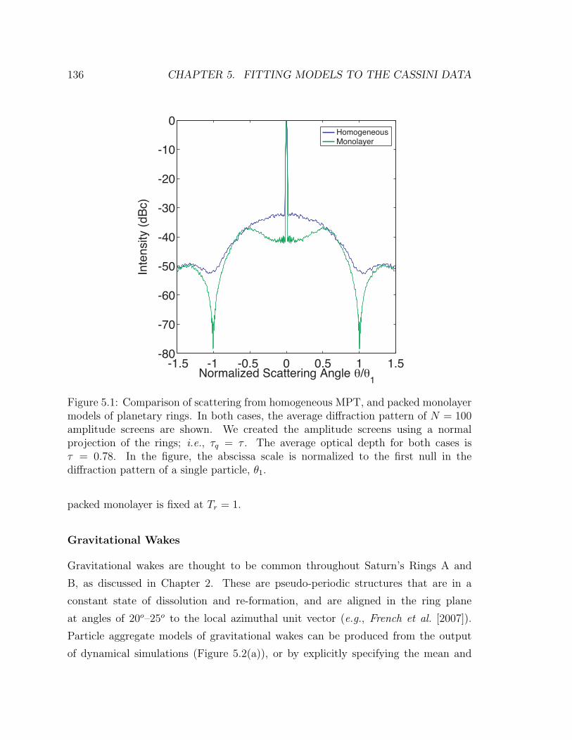
136 CHAPTER 5. FITTING MODELS TO THE CASSINI DATA
-1.5 -1 -0.5 0 0.5 1 1.5-80
-70
-60
-50
-40
-30
-20
-10
0
Normalized Scattering Angle θ/θ1
Inte
nsity
(dB
c)HomogeneousMonolayer
Figure 5.1: Comparison of scattering from homogeneous MPT, and packed monolayermodels of planetary rings. In both cases, the average diffraction pattern of N = 100amplitude screens are shown. We created the amplitude screens using a normalprojection of the rings; i.e., τq = τ . The average optical depth for both cases isτ = 0.78. In the figure, the abscissa scale is normalized to the first null in thediffraction pattern of a single particle, θ1.
packed monolayer is fixed at Tr = 1.
Gravitational Wakes
Gravitational wakes are thought to be common throughout Saturn’s Rings A and
B, as discussed in Chapter 2. These are pseudo-periodic structures that are in a
constant state of dissolution and re-formation, and are aligned in the ring plane
at angles of 20o–25o to the local azimuthal unit vector (e.g., French et al. [2007]).
Particle aggregate models of gravitational wakes can be produced from the output
of dynamical simulations (Figure 5.2(a)), or by explicitly specifying the mean and

5.2. MICROSTRUCTURE MODELING TECHNIQUES 137
standard deviation of wake spacing and orientation (cant angle) as shown in Figure
5.3.
In Figure 5.2, we show amplitude screens and diffraction patterns that we created
using the results of dynamical simulations performed by Heikki Salo at the University
of Oulu [Salo, 2006]. Salo’s simulations produced a time-domain evolution of the
position and velocity of 5330 1.66-m radius ring particles as the particles orbit Saturn.
Other physical parameters specified in the model are surface mass density σρ = 500
kg m−2, and volume mass density ρ = 450 kg m−3 (σρ and ρ are described in more
detail in Appendix A). Initially, the particles are homogeneously distributed within
the 300× 300× 55 m simulation volume; the volume is centered in the ring plane at
a distance of 100,000 km from Saturn’s center.
During the simulation, Salo’s code outputs the position of all particles contained
within the simulation volume at the end of each of 100 successive orbits of Saturn. For
the given input parameters, the homogeneous initial distribution of particles evolves
to a distribution that contains distinct wakes, as seen in Figure 5.2(a), by the tenth
orbit. A detailed description of the simulation is given in Salo [1995].
Salo shared with us the files containing the position of each of the 5330 particles
at the end of each of 100 consecutive simulated orbits of Saturn (i.e., 100 files in
total). We used these files to create N = 90 amplitude screens, corresponding to the
particle aggregates defined by Salo’s files for orbits 11–100, and in which gravitational
wakes are evident. Figure 5.2(a) is an amplitude screen produced from one of Salo’s
particle position files. In Figure 5.2(b) we show the average diffraction pattern of
N = 90 vignettes. Figure 5.2(c) is a plot of the diffracted signal intensity along the
dashed line shown in white in Figure 5.2(b), which is oriented at a cant angle of
approximately 25o to the u-axis, showing the enhanced scattering in the very near
forward direction that is characteristic of wakes. Figures 5.2(b)–(c) show diffraction
in the spatial frequency domain; a method for transforming to the Doppler frequency
domain and comparing the results with Cassini data is the subject of Section 5.3.
We also represent gravitational wakes using the parameterized, statistically gen-
erated particle aggregate model shown in Figure 5.3. The model is specified by its
optical depth (either τ or τq), the mean λgr and standard deviation σgr of the wake

138 CHAPTER 5. FITTING MODELS TO THE CASSINI DATA
x (meters)
y (meters)
-150-100
-500
50100
150-150
-100
-50 0
50
100
150
Spatial F
requency (1/m)
Spatial Frequency (1/m)
-1-0.8
-0.6-0.4
-0.20
0.20.4
0.60.8
1
-1
-0.8
-0.6
-0.4
-0.2 0
0.2
0.4
0.6
0.8 1
-0.25-0.2
-0.15-0.1
-0.050
0.050.1
0.150.2
0.25-40
-35
-30
-25
-20
-15
-10 -5 0
Spatial F
requency (1/m)
Intensity (dB)
(a)(b)
(c)
~25
o
Figu
re5.2:
Diffraction
signatu
reof
gravitation
alwakes.
Grav
itational
wake
structu
resare
clearlyvisib
lein
(a),which
show
sa300×
300meter
vign
etteof
therin
gsgen
erateddurin
gdynam
icalsim
ulation
s.Thesim
ulated
physical
ringprop
ertiesare
typical
ofSatu
rn’sRingA
(τ=
0.5;surface
mass
density
σρ=
500kgm
−2;rin
gdensity
ρ=
450kgm
−3;particle
radiusa=
1.66m);see
Appendix
A.In
(a),they-ax
isisalign
edwith
thelocal
Keplerian
motion
ofarin
gparticle.
Wecom
puted
thediffraction
pattern
Uof
90indep
endentam
plitu
descreen
s(of
which
(a)is
one);
theinten
sity-avaraged
(I=
UU
∗)diffraction
pattern
ofthose
screensis
show
nin
(b).
Thesign
ature
ofindividual
particles
ispreserved
inthelarge-scale
diffraction
pattern
(i.e.,theAiry
disk
isvisib
lein
(b);
seealso
Figu
re3.9)),
while
thediffraction
signatu
reof
thewakes
isvisib
leas
asm
all,brigh
tsm
earat
thecen
terof
theplot.
Thediffracted
field
inten
sityalon
galin
e—orien
tedat≈
25oas
show
nin
(b)—
throu
ghwake
signatu
rein
the2D
diffraction
pattern
isplotted
in(c).
Note
thesim
ilaritybetw
eentheplot
(c)an
dthemeasu
redspectru
mshow
nin
Figu
re4.3.
Thetw
osm
allpeak
son
either
sideof
thecen
tralpeak
inthediffraction
pattern
indicate
thewakes’
mean
structu
ralperio
d,while
thecan
tan
gleof≈
25oistheaverage
wake
cantan
glewith
respect
totheazim
uthal
unitvector
φin
therin
gs(i.e.,
with
respect
toyin
thisfigu
re).Theparticle
distrib
ution
swere
prov
ided
byHeik
ki
Salo,
University
ofOulu.

5.2. MICROSTRUCTURE MODELING TECHNIQUES 139
Radial linefrom Saturnbarycenter
O
ugr
Gravitational Wakes orPeriodic Microstructure
grλgrφ
urro
φ
Figure 5.3: Statistically generated amplitude screen model of gravitational wakes orperiodic microstructure, showing placement in the ring plane. The vector ro definesthe position of the ring piercing point O relative to Saturn’s barycenter; ur is the unitvector pointing from Saturn’s barycenter to the RPP. The orientation of the structurein the ring plane is specified by ugr (alternatively by φgr). The mean structuralperiod λgr is shown; its standard deviation σgr (not labeled) controls the width of thenormally-distributed particle clusters that form the wakes and/or PM.

140 CHAPTER 5. FITTING MODELS TO THE CASSINI DATA
Radial linesfrom Saturnbarycenter
O
ugr
ur
Periodic Microstructure
gr
gr
T(r)
ro
r
ˆ
Figure 5.4: Deterministic sinusoidal transmittance amplitude screen model of periodicmicrostructure, showing placement in the ring plane. The screen transmittance T (r)is defined in eq. 5.1, where r is a position vector originating at Saturn’s barycenter,as is ro which defines the RPP. The angle between r and ro is exaggerated here, forclarity. All other labels and geometry are as in Figure 5.3 (note that σgr is not definedin this model).
spacing, and the orientation or cant angle φgr of the wakes in the ring plane, relative
to the azimuthal unit vector φ. This wake model is further constrained by specifying
the ring thickness Tr or the packing fraction fvol. We populate a ring slab volume
according to the defined statistics, and the number of particles Np is adjusted iter-
atively in our model until the output of eq. (3.73) equals the defined optical depth
specification.

5.2. MICROSTRUCTURE MODELING TECHNIQUES 141
Periodic Microstructure
With the Cassini radio occultation experiment, we have detected periodic microstruc-
ture at five distinct locations in the rings [Thomson et al., 2007]. Colwell et al. [2007]
and Sremcevic et al. [2009] used the Cassini ultraviolet imaging spectrograph (UVIS)
to detect PM in regions of Rings A and B, and reported results that are consistent
with our observations.
As was the case for gravitational wakes, particle aggregate models of PM are
produced either by using the output of dynamical simulations to determine the ring
particle locations in the ring plane, or by using the statistically generated parameter-
ized model shown in Figure 5.3. For PM investigations, the particle aggregate model
is useful for investigating the impact of the orientation angle φgr and ring thickness Tr
on the observed optical depth. However, if our goal is simply to identify the geometry
required to produce the first-order diffraction lobes that are the hallmark of PM (e.g.,
Figure 4.5(a)–(b)), then we only need a model that is specified by λgr and φgr.
For this, we define an amplitude screen with transmittance T (r), containing a
deterministic sinusiodal amplitude component. The model is completely specified
by four parameters, which are: i) the average transmittance T of the screen, ii) the
sinusoidal amplitude ∆T of the variation in screen transmittance, iii) the structural
period λgr, and iv) the orientation vector ugr (or alternatively, φgr), which we define
relative to an axisymmetric orientation. With this,
T (r) = T +∆T cos
(2π(r · ugr)
λgr
)(5.1)
where r is the radius vector from Saturn’s center to points within the amplitude
screen; see Fig. 5.4 for the screen geometry. The parameter T is determined by the
observed normal optical depth τ ,
T = exp
(−τ
2µo
)(5.2)
where µo = sinB, and B is the ring opening angle (see Figure 5.8; cf. Fig. 15 of Tyler
[1987]). The parameter ∆T is determined from the observations according to,
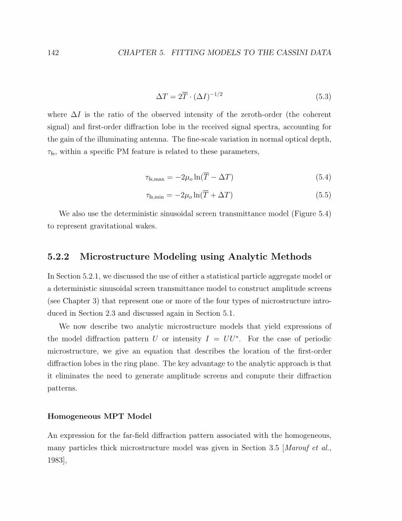
142 CHAPTER 5. FITTING MODELS TO THE CASSINI DATA
∆T = 2T · (∆I)−1/2 (5.3)
where ∆I is the ratio of the observed intensity of the zeroth-order (the coherent
signal) and first-order diffraction lobe in the received signal spectra, accounting for
the gain of the illuminating antenna. The fine-scale variation in normal optical depth,
τfs, within a specific PM feature is related to these parameters,
τfs,max = −2µo ln(T −∆T ) (5.4)
τfs,min = −2µo ln(T +∆T ) (5.5)
We also use the deterministic sinusoidal screen transmittance model (Figure 5.4)
to represent gravitational wakes.
5.2.2 Microstructure Modeling using Analytic Methods
In Section 5.2.1, we discussed the use of either a statistical particle aggregate model or
a deterministic sinusoidal screen transmittance model to construct amplitude screens
(see Chapter 3) that represent one or more of the four types of microstructure intro-
duced in Section 2.3 and discussed again in Section 5.1.
We now describe two analytic microstructure models that yield expressions of
the model diffraction pattern U or intensity I = UU∗. For the case of periodic
microstructure, we give an equation that describes the location of the first-order
diffraction lobes in the ring plane. The key advantage to the analytic approach is that
it eliminates the need to generate amplitude screens and compute their diffraction
patterns.
Homogeneous MPT Model
An expression for the far-field diffraction pattern associated with the homogeneous,
many particles thick microstructure model was given in Section 3.5 [Marouf et al.,
1983],
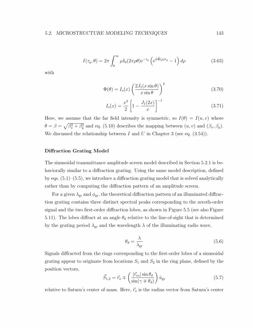
5.2. MICROSTRUCTURE MODELING TECHNIQUES 143
I(τq, θ) = 2π
∫ ∞
0
ρJ0(2πρθ)e−τq(ew
˜Φ(ρ)τq − 1)dρ (3.63)
with
Φ(θ) = Io(x)
(2J1(x sin θ)
x sin θ
)2
(3.70)
Io(x) =x2
2
[1− J1(2x)
x
]−1
(3.71)
Here, we assume that the far field intensity is symmetric, so I(θ) = I(u, v) where
θ = β =√β2x + β2
y and eq. (5.10) describes the mapping between (u, v) and (βx, βy).
We discussed the relationship between I and U in Chapter 3 (see eq. (3.54)).
Diffraction Grating Model
The sinusoidal transmittance amplitude screen model described in Section 5.2.1 is be-
haviorally similar to a diffraction grating. Using the same model description, defined
by eqs. (5.1)–(5.5), we introduce a diffraction grating model that is solved analytically
rather than by computing the diffraction pattern of an amplitude screen.
For a given λgr and φgr, the theoretical diffraction pattern of an illuminated diffrac-
tion grating contains three distinct spectral peaks corresponding to the zeroth-order
signal and the two first-order diffraction lobes, as shown in Figure 5.5 (see also Figure
5.11). The lobes diffract at an angle θd relative to the line-of-sight that is determined
by the grating period λgr and the wavelength λ of the illuminating radio wave,
θd =λ
λgr
(5.6)
Signals diffracted from the rings corresponding to the first-order lobes of a sinusoidal
grating appear to originate from locations S1 and S2 in the ring plane, defined by the
position vectors,
S1,2 = ro ∓( |rco| sin θdsin(γ ∓ θd)
)ugr (5.7)
relative to Saturn’s center of mass. Here, ro is the radius vector from Saturn’s center

144 CHAPTER 5. FITTING MODELS TO THE CASSINI DATA
dd
d
ZerothOrder
FirstOrder
FirstOrder
Incident Plane Wave
Rings (edge-on)
Observer
OS1 S2grugr
= 2 kk
Figure 5.5: Properties of a sinusoidal diffraction grating. First-order lobes arediffracted at an angle θd with respect to the incident plane wave vector k, in theplane containing both k and the grating orientation vector ugr. Energy diffractedtowards the observer by the first-order lobes originates at S1 and S2, which are alongthe line of diffraction grating lobes, defined as the intersection of the plane containingk and ugr, and the ring plane (see also Figure 5.6). The line of diffraction gratinglobes is also the line oriented along ugr that includes point O. This description is alsovalid for signals originating at the observer and arriving at the distant source of theilluminating plane wave in this figure, by reciprocity. Compare with Figures 5.6 and5.12.

5.2. MICROSTRUCTURE MODELING TECHNIQUES 145
To Earth
Line ofdiffraction
grating lobes
γO
Cassini
S1
S2
dθ
dθ
dθ dθ
ugr
uE
uE
uEuE
Figure 5.6: Diffraction grating and Cassini observation geometry. The view shownis drawn in the plane that contains ugr and uE (note that uE = k); the line ofdiffraction grating lobes is in the plane of the page. The ring plane, containing asinusoidal diffraction grating parameterized by λgr and ugr, protrudes from the pageat an unspecified angle. Angle γ is between −uE and ugr. Point O defines the RPP;S1 and S2 are points in the ring plane where Cassini signals diffracted through anangle θd are redirected towards Earth along uE. Compare with Figures 5.5, and 5.12.

146 CHAPTER 5. FITTING MODELS TO THE CASSINI DATA
to the ring intercept point O, rco is the vector from the Cassini spacecraft to point O
(rco = ro − Rc; see Figure 4.1 or 5.12), and γ = cos−1(−uE · ugr); see Figure 5.6.
5.3 Comparing Model Behavior with Radio Occul-
tation Measurements
We match power spectral features derived from the diffraction pattern of presumed
ring microstructure models with key features in the power spectrum of signals received
from Cassini, which contain the diffraction signature of the true ring microstructure.
Our approach comprises two main techniques: a general technique, and a faster,
simpler technique that is specific to periodic microstructure. We used the second
technique to produce the estimates of the physical dimensions of PM in the rings
that we present in Chapter 6.
With either the general or PM-specific approach, we adopt the implicit assumption
that the nature of the microstructure is statistically stationary over multiple Cassini
observations. In our case, the stationary assumption spans the May–August 2005
timeframe of the observations we use in our analysis.
The methods we describe in this chapter require accurate estimates of the position
and velocity of Cassini, Saturn, and the Earth in order to reconstruct the observa-
tional geometry and to calculate associated quantities—such as ro and fD—required
in the analysis. To this end, we use the SPICE information system, which is provided
to the scientific community and maintained by the NASA/JPL Navigation and An-
cillary Information Facility (NAIF). SPICE includes a large suite of software (mostly
in the form of subroutines) to assist scientists in planning and interpreting scientific
observations from space-based instruments. The Cassini project office releases files
called SPICE kernels on a regular basis, which contain the best estimate of Cassini’s
actual trajectory during a fixed range of dates. NAIF also releases kernel files for
all major solar system objects (planets, moons, etc.). We incorporated SPICE sub-
routines in our code in order to read SPICE kernel files and compute highly-resolved
estimates of the Cassini radio occultation geometry.

5.3. COMPARING MODEL BEHAVIOR WITH MEASUREMENTS 147
5.3.1 General Approach
In this section, we outline a general approach that applies to all models that use ring
particle aggregates to represent ring microstructure. We describe an iterative fitting
procedure for estimating ring microstructure at a single location ro in the rings. The
iterative process is repeated for multiple ro to resolve microstructure features that
span a range of ring radii.
To be clear, a full development and application of the general approach is beyond
the scope of this dissertation. However, the general approach provides an excellent
pedagogical framework with which to present the basic concepts and procedures that
are essential to the techniques we use to fit models of periodic microstructure to the
Cassini data. Our PM model fitting techniques derive from the general method but
are specialized for PM analysis and therefore limited by comparison, as we describe
in Section 5.3.2. A complete development of the general approach is an important
future step in the analysis of Cassini radio occultation data to investigate the nature
of ring microstructure.
Generating the Diffraction Screens: Particle Aggregate Models
We begin with a region of the rings containing microstructure that we wish to investi-
gate, and we choose a particle aggregate model from those introduced in Section 5.2.1
to fit to the measured Cassini radio occultation data. For each unique set of model
parameters (i.e., unique values of parameters τ , λgr, σgr, φgr, Tr, etc.), we generate N
amplitude screens, each of which are unique instantiations or vignettes corresponding
to a single statistical description of the rings.
Each vignette is generated as shown in Figure 3.1—by projecting the shadows of
particles into a plane perpendicular to the unit wave vector k = uE. Particle positions
in our model use the coordinate system introduced in Figures 4.1 and 4.2, where z
is Saturn’s pole vector, x is the unit vector projection of uE in the ring plane, and
y = z× x. The position (x, y) of particles is preserved in the creation of the amplitude
screen—thus ∆x = ∆ysinB
for amplitude screens constructed using an equal number of
pixels in x and y. Figure 5.7 depicts the projection process as it pertains explicitly

148 CHAPTER 5. FITTING MODELS TO THE CASSINI DATA
Incident Radio Wave
zx
y
Amplitude Screen
Microstructure M
odel of Saturn's R
ings
(edge-on view)
y
Am
plitu
de S
cree
n
Proj
ectio
n
B x
= 2 kk
Figure 5.7: Constructing amplitude screens from models of ring microstructure. Thegeneral procedure for screen construction is explained in Chapter 3. Significant ringparticle overlap is evident along the x-dimension in the amplitude screen, due to theacute ring opening angle. If the two dimensions of the amplitude screen comprise thesame number of pixels, then ∆x = ∆y
sinB, where B is the ring opening angle defined in
Section 1.2.
to the rings.
There is often a tradeoff to be made between resolving the diffraction signature of
individual particles and that of the structures formed by those particles, as discussed
in Section 3.2.4. Figure 5.2(b) illustrates the problem: when the microstructure has
characteristic dimensions that are many particles in extent, the spectral diffraction
signature of the microstructure exists on a proportionally smaller scale that the par-
ticles. This is due to the inverse relationship that exists between dimensions in the
spatial domain and the spatial frequency domain.
For microstructure vignettes that are hundreds of particles long in x and/or y, it is
impractical to resolve the diffraction pattern of both the particles and the structure
since the small values of ∆x and ∆y required quickly lead to very long numerical
transforms. Depending on the nature of the microstructure, it may be necessary to
increase ∆x and ∆y in order to properly sample the structure, thus decreasing the
spatial sampling frequency fsx (fsy) and the frequency-domain resolution ∆fx (∆fy).
In the limit, we can reduce the spatial resolution to one pixel per particle, focussing
in on the diffraction signature of microstructure in the process.

5.3. COMPARING MODEL BEHAVIOR WITH MEASUREMENTS 149
We compute the diffraction pattern of the N amplitude screens using the methods
described in Chapter 3. We apply a 2D Hamming function to each amplitude screen
a priori to mitigate the spectral leakage effects associated with the finite length of the
FFT. We average the N diffraction patterns incoherently (cf., eq. (3.54)) to obtain,
U(u, v) =
√√√√ 1
N
N∑i=1
Ui(u, v)U∗i (u, v) (5.8)
thus creating a single diffraction pattern U(u, v), that represents the statistical be-
havior of the particular model type (wakes, PM, etc.) and unique parameter values.
We choose N large enough to reduce the statistical noise in the spatial frequency
domain, inherently introduced by amplitude screen models that contain statistically-
defined dimensions. A possible criterion for N is to require the maximum difference
between the diffraction patterns produced by averaging (N − 1) and N diffraction
patterns to be less than a small value ε,
ε ≥∣∣∣∣∣ 1N
N∑i=1
U2i (u, v)−
1
N − 1
N−1∑i=1
U2i (u, v)
∣∣∣∣∣max
(5.9)
where ε is on the order of a few percent, and U2 = UU∗.
We apply a linear paraxial transformation to map the spatial frequency domain
U(u, v) to the angular frequency domain U(βx, βy),
βx = λu βy = λv (5.10)
where λ is the wavelength of the Cassini signal used in the analysis (either 13 cm, 3.6
cm, or 0.94 cm; see Section 4.1).
Generating the Diffraction Screens: Screen Transmittance Models
The sinusoidal screen transmittance model depicted in Figure 5.4 is defined determin-
istically, not statistically. In this case we compute U(βx, βy) using a single amplitude
screen for each unique set of parameter values (i.e., N = 1). Otherwise, the procedure

150 CHAPTER 5. FITTING MODELS TO THE CASSINI DATA
is exactly the same as that described above for particle aggregate models.
Doppler Signal Synthesis
The incoherent or scattered signal spectrum is a superposition of signals forward-
scattered or diffracted towards Earth from regions in the rings that are illuminated by
the Cassini high-gain antenna. We receive these signals at Earth, and each is Doppler-
shifted with respect to the transmitted signal frequency as discussed in Section 4.1.
To test a presumed model of ring microstructure, we must synthesize a received
signal spectrum Is(fD) that corresponds to the average diffraction pattern U(βx, βy)
of the specific model, and which is consistent with the observational geometry of
the actual experiment. Reconstructing the observational geometry ensures a correct
mapping of Doppler frequency fD to precise locations in the ring plane.
Figures 5.8 and 5.9 show the geometry and general approach of the Doppler syn-
thesis method. A fraction of the Cassini transmitted signal power that propagates
along up to illuminate point P is diffracted through an angle βp to propagate along
uE towards Earth. For P located at a point (xi, yj) in the ring plane (the xyz coordi-
nate system is explained in Figure 4.1), the signal intensity scattered from P towards
Earth depends on both the diffraction pattern U(βxi, βyj) of the rings and on the
incident power illuminating the rings, which in turn is a function of the gain of the
Cassini high-gain antenna (HGA),
Is(βx, βy) = G(βx, βy) · U2(βx, βy) (5.11)
Is(βx, βy) is the normalized intensity of signals scattered to Earth from points in the
rings defined by βx and βy, and G(βx, βy) = G(β) is the pattern gain of the Cassini
antenna (cf., eq. (3.70)),
G(β) =
[2J1 (ηka sin β)
ηka sin β
]2(5.12)
where β =√β2x + β2
y . Here, J1 is the first-order Bessel function of the first kind, a is
the radius of the Cassini high-gain antenna (a = 2 meters), k = 2π/λ, and η is a factor

5.3. COMPARING MODEL BEHAVIOR WITH MEASUREMENTS 151
uE
y
x
x
y
z
x
y
z
ToCassini
OB
Locus ofconstant p
(xi,yj)
up
Negative Doppler Positive Doppler
Figure 5.8: Diffraction and Doppler geometry in the ring plane. Radio waves prop-agating along up from Cassini intercept the rings at point P , located at (xi, yj) inthe ring plane. Microstructure present in the rings in the vicinity of P diffracts aportion of the transmitted signal energy towards Earth along uE. The diffraction
angle βp = cos−1(up · uE) =√β2xi+ β2
yjis subtended between up and uE. The angle
αxi= B+βxi
is formed by projecting the ray up linking Cassini and point P at (xi, yj)into the xz plane; similarly, βyj is formed by projecting up into the yz plane, as shown.Angle B is the rings opening angle, and the subscripts i and j have been droppedfrom αxi
and βyj in the figure, for brevity. For a given observational geometry, sig-nals scattered towards Earth from point P map to a particular Doppler frequencyfD. Doppler values are represented graphically in the figure by a color spectrum asin Figure 4.2, but are not to scale. The line-of-sight ray linking Cassini and Earthpierces the rings at point O. The reader is referred to Figure 4.1 for a more generalview of the geometry shown in detail in this figure.

152 CHAPTER 5. FITTING MODELS TO THE CASSINI DATAD
iffra
ctio
n A
ngle
βx
0
0Diffraction Angle βy
xi
yj
x
yz
yβ
xβ
yj, βxi
β( )
0
0
Locus ofconstant βp
Negative Doppler Positive Doppler
Figure 5.9: Determining the magnitude U(βxi, βyj) and Doppler frequency fDp of sig-
nals received from point P in the ring plane. Radio waves transmitted by Cassini and
illuminating the rings at point P at (xi, yj) are diffracted by an angle βp =√
β2xi+ β2
yj
towards the Earth, as shown in Figure 5.8. For a given observational geometry, andan assumed model of ring microstructure producing an average diffraction patternU(βx, βy), each ordered pair (βxi
, βyj) maps to a single point (xi, yi) in the ring plane.Signals from P are received at a relative magnitude Is(βxi
, βyj), defined in eq. (5.11),and at the Doppler frequency associated with P . Contributions from all points inthe rings are used to synthesize a received signal spectrum Is(fD) associated with aparticular model of ring microstructure.
that accounts for the deliberate de-focussing of the Ka-band signal in the HGA. For
Cassini, η = 1 for X- and S-band transmissions, and η = 0.806 for Ka-band, yielding

5.3. COMPARING MODEL BEHAVIOR WITH MEASUREMENTS 153
a half-power beamwidth of βHP|Ka = 0.0015 radians.
Since each unique ordered pair (βxi, βyj) maps to a single point (xi, yj) in the
ring plane, and each point in the ring plane has an associated Doppler frequency fD,
we can synthesize a received signal spectrum that corresponds to a specific model of
ring microstructure and occultation signal wavelength—represented by Is(βx, βy)—
and to a specific observational geometry. For each value of (βx, βy), we compute the
corresponding position vector up (see Figure 5.8) by first finding the vectors x and y
that locate the point (x, y) relative to the RPP,
x =|rco| sin(βx)
cosBx (5.13)
y = |rco| tan(βy)y (5.14)
where x and y are as shown in Figure 4.1, B is the ring opening angle, and rco was
introduced in eq. (5.7). The vector from Cassini to (x, y) is given by rp = rco+x+ y,
and it follows that up is defined as,
up = |rp|−1rp (5.15)
For homogeneous ring models, we compute the Doppler frequency fD associated with
each (βx, βy), using the computed value of up in eq. (4.1). For other models of ring
microstructure we use modified formulae to compute fD, which we discuss below and
define in eqs. (5.17)–(5.17).
We store the numerical values of Is(βx, βy) and the associated Doppler values fD
in corresponding K ×K matrices, and then collapse the matrices into two vectors of
length 1 × K2. We sort values contained in the Doppler vector in ascending order,
and commensurately re-order the Is vector. Finally, a histogram algorithm is used to
sum the Is vector in Doppler bins that are sized to match the frequency bin size of
the measured Cassini signal, thus producing the synthesized received signal spectrum
Is(fD).

154 CHAPTER 5. FITTING MODELS TO THE CASSINI DATA
Next page.
Figure 5.10: Synthesis of Is(fD) from models of ring microstructure. Panels A–Dshow single instantiations of amplitude screens representing a particular microstruc-ture model, along with the Doppler power spectra Is(fD) that we synthesized fromthe average of N = 100 unique diffraction patterns U(βx, βY ). The different mi-crostructure models shown represent a range of simulated optical depths. Shown areA a homogeneous MPT ring model (τq = 3.26, Np = 9870, Tr = 43), B a packedmonolayer model (τq = 1.53, Np = 4000, Tr = 1), C gravitational wakes (τq = 0.60,Np = 5330, Tr = 17), and D periodic microstructure (τq = 0.15, Np = 2170, Tr = 6).In all panels, Is(fD) is synthesized at X-band, assuming the REV 7 ingress geom-etry and |ro| = 123,100 km from Saturn’s barycenter. The bias of all synthesizedDoppler spectra have been chosen to facilitate comparison with the power spectra ofmicrostructure contained in Figures 4.5 and 6.4. The coherent signal component isnot included in Is(fD). In panel B, the near-forward extinction associated with scat-tering from packed monolayers (shown in Figure 5.1) is spread over roughly ±2 kHz(see the 3 dB beam pattern in Figure 4.2), and therefore is not distinctly seen in oursynthesis. Note the scattering enhancement in the near-forward direction producedby gravitational wakes, panel C, as compared with the more superimposed sidelobenature produced by periodic microstructure, panel D. These results are preliminaryand are intended for qualitative comparisons and/or illustrative purposes only.

5.3. COMPARING MODEL BEHAVIOR WITH MEASUREMENTS 155
meters
064 -64 -6
464
0m
eter
s-1
01
510152025303540
Fre
quen
cy (
kHz)
Intensity (dB)
meters 0
150
-150 -1
5015
00
met
ers
510152025303540
-10
1
Intensity (dB)
Fre
quen
cy (
kHz)
meters
0
150
-150 -1
5015
00
met
ers
510152025303540
-10
1
Intensity (dB)
Fre
quen
cy (
kHz)
510152025303540
-10
1
Intensity (dB)
meters 0
128
-128 -1
2812
80
met
ers
Fre
quen
cy (
kHz)
BA
DC
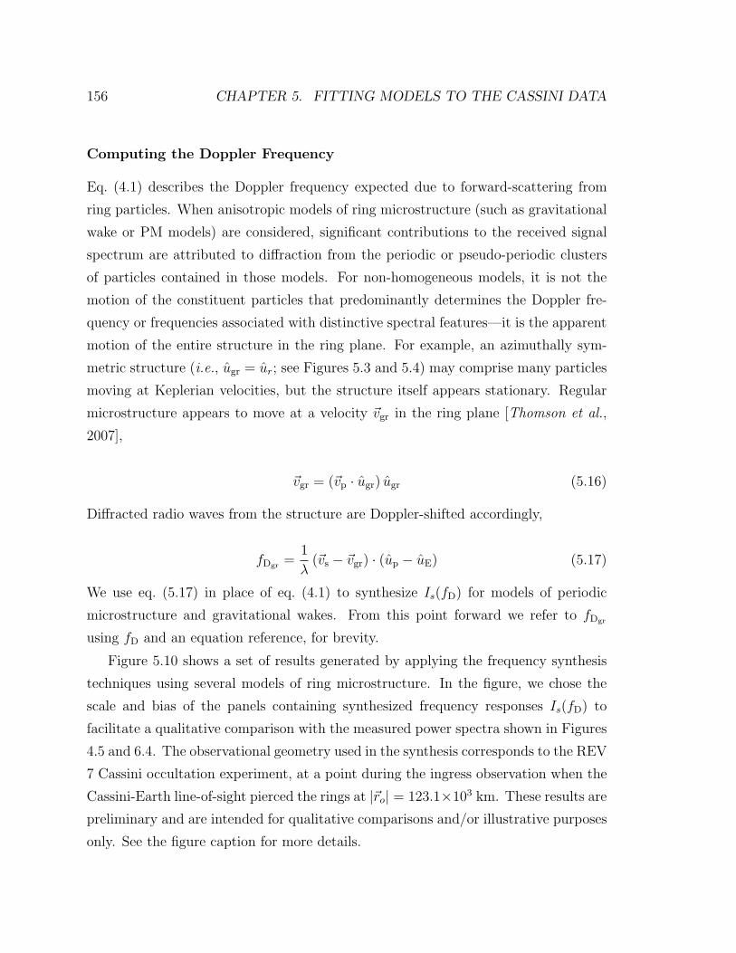
156 CHAPTER 5. FITTING MODELS TO THE CASSINI DATA
Computing the Doppler Frequency
Eq. (4.1) describes the Doppler frequency expected due to forward-scattering from
ring particles. When anisotropic models of ring microstructure (such as gravitational
wake or PM models) are considered, significant contributions to the received signal
spectrum are attributed to diffraction from the periodic or pseudo-periodic clusters
of particles contained in those models. For non-homogeneous models, it is not the
motion of the constituent particles that predominantly determines the Doppler fre-
quency or frequencies associated with distinctive spectral features—it is the apparent
motion of the entire structure in the ring plane. For example, an azimuthally sym-
metric structure (i.e., ugr = ur; see Figures 5.3 and 5.4) may comprise many particles
moving at Keplerian velocities, but the structure itself appears stationary. Regular
microstructure appears to move at a velocity vgr in the ring plane [Thomson et al.,
2007],
vgr = (vp · ugr) ugr (5.16)
Diffracted radio waves from the structure are Doppler-shifted accordingly,
fDgr =1
λ(vs − vgr) · (up − uE) (5.17)
We use eq. (5.17) in place of eq. (4.1) to synthesize Is(fD) for models of periodic
microstructure and gravitational wakes. From this point forward we refer to fDgr
using fD and an equation reference, for brevity.
Figure 5.10 shows a set of results generated by applying the frequency synthesis
techniques using several models of ring microstructure. In the figure, we chose the
scale and bias of the panels containing synthesized frequency responses Is(fD) to
facilitate a qualitative comparison with the measured power spectra shown in Figures
4.5 and 6.4. The observational geometry used in the synthesis corresponds to the REV
7 Cassini occultation experiment, at a point during the ingress observation when the
Cassini-Earth line-of-sight pierced the rings at |ro| = 123.1×10³ km. These results are
preliminary and are intended for qualitative comparisons and/or illustrative purposes
only. See the figure caption for more details.

5.3. COMPARING MODEL BEHAVIOR WITH MEASUREMENTS 157
5.3.2 Periodic Microstructure
For the case of periodic microstructure, the sharp first-order diffraction lobes char-
acteristic of PM (see the simulation results shown in Figure 5.11) allow us to greatly
simplify the modeling procedure. In this case, synthesis of Is(fD) is not required—
rather, we need only find the two Doppler frequencies, fD1 and fD2, corresponding to
the peaks of the first-order diffraction lobes.
Sinusoidal Transmittance Model
We use the first-order diffraction lobe peaks β1 and β2 evident in the angular frequency
domain of the sinusoidal transmittance model to compute the diffraction lobe peaks
fD1 and fD2 in the Doppler frequency domain. Figure 5.11 shows an example of
a diffraction pattern U(βx, βy) generated from a sinusoidal transmittance model of
periodic microstructure, as detailed in Section 5.2.1. We use a peak-finder algorithm
to uniquely determine the two first-order diffraction lobe peaks in U(βx, βy), which we
show located at (βx1 , βy1) and (βx2 , βy2) in the figure. We find the associated Doppler
frequencies fD1 and fD2 directly using the approach described in eqs. (5.13)–(5.15)
above; eq. (5.17) is used to compute the specific Doppler frequencies.
Analytic Diffraction Grating Model
The procedure for finding fD1 and fD2 is even simpler for the (analytic) diffraction
grating model, which is depicted in Figure 5.12. In this case, there is no need to
generate any amplitude screens. For a specific observational geometry, we compute
S1 and S2 using eq. (5.7). Then rpi = rco + Si, and we compute up1 and up2 using eq.
(5.15). Substituting into eq. (5.17) yields fD1 and fD2, respectively.

158 CHAPTER 5. FITTING MODELS TO THE CASSINI DATA
-5000
0
500050000-5000
Y (meters)
X (
met
ers)
-0.0072
0.00720.0072-0.0072
βx
(rad
ians
)
βy (radians)
0
0
β1
β2
(a) (b)
Figure 5.11: An example of (a) the sinusoidal transmittance model of periodic mi-crostructure, λgr = 100 m, and (b) its associated diffraction pattern U(βx, βy).Values of β are computed for an X-band signal, λ = 3.6 cm. Note the spacing∆β = |β1 − β2| = 2so, where so = λ−1
gr .
5.4 Least-Squares Fitting of Model Parameters to
the Data
We use an iterative least-squares fitting approach to determine the optimal set of
model parameters that fit the synthesized frequency spectrum to the frequency spec-
trum of the Cassini data. For periodic microstructure models, we only fit at two
locations in the spectrum. Specifically, we fit the measured first-order diffraction lobe
frequencies, designated fm1 and fm2, to the sidelobe frequencies in the synthesized
spectrum, fD1 and fD2. In this case, it is not necessary to synthesize Is(fD). For
the PM model case, we now describe the process of fitting model parameters to the
experimental data.

5.4. LEAST-SQUARES MODEL FITTING TO THE DATA 159
Periodicmicrostructure
φgr
λgr
ugr
ur
S1
S2
OuE
vs
ugr
S1
uE
S2
O
2θd
θ
θ
γ
Rc
ro
uφ
Antenna footprinton Rings
(a) (b)
Negative Doppler Positive Doppler
Figure 5.12: Diffraction grating model of periodic microstructure in the rings. (a)Line-of-sight ray linking Cassini and Earth is directed along uE and pierces the ringplane at point O; ugr is in the plane of the rings, and defines the orientation of theperiodic structure. Points S1 and S2 correspond to locations in the ring plane wherefirst-order diffraction grating lobes of the structure originate and propagate along uE
to the Earth-based receiver. The grating lobes are directed at angle ±θd relative touE. All angles shown are in the plane defined by uE and ugr. Color within the antennafootprint represents variations in the Doppler shift of signals scattered to Earth bythe rings; the antenna footprint size is exaggerated for clarity. (b) The grating isrepresented by parallel green lines in this schematic top view of the rings. Signalsdiffracted to Earth from S1 and S2 are Doppler-shifted by fD1 and fD2 relative to thesignal along the line-of-sight, represented by the colors at S1 and S2. ur = |ro|−1ro isthe radial unit vector pointing from the center of Saturn to O.
5.4.1 Fitting Models of Periodic Microstructure
Figure 5.13 shows the spectrum of the Ka-band Cassini received signal recorded during
the REV 7 ingress occultation observation, May 3, 2005. The spectrum shown is an
average over a 25-km range along the occultation track, centered on a point ro =

160 CHAPTER 5. FITTING MODELS TO THE CASSINI DATA
123,249 km from Saturn’s center.
For each radial location |ro| in the rings for which we wish to fit a model of
periodic microstructure, we must first determine the actual first-order diffraction lobe
frequencies, fm1 and fm2, from the measured Cassini radio occultation data. Using a
four-parameter Gaussian model,
F (f ;P i) = Ci exp
(−(f − fmi)
2
2σ2i
)+ Foi (5.18)
we adjust the amplitude Ci, standard deviation σi, bias Foi, and first-order diffraction
lobe frequencies fmi, where i = 1, 2, to fit the measured data as shown in Figure 5.13.
The vector P i = [Ci fmi σi Foi] defines the model’s independent fitting parameters.
The Gaussian model (eq. (5.18)) is fit to the Cassini spectral data using a least-squares
optimization routine that employs a Levenberg-Marquardt algorithm to minimize the
sum-of-squares error Γ(P ) according to,
Γ(P ) =K∑k=1
[I(fk)− F (fk;P )
]2(5.19)
where I(fk) is the intensity of the received signal spectrum at frequency fk, and
F (fk;P ) is the parameterized function that minimizes Γ(P ); in this case, given by
eq. (5.18). Here, we limit the range of frequencies, f1 to fK , such that F (fk;P ) is
optimized to fit either the upper or lower diffraction lobe—never both at once. This
is depicted in Figure 5.13 by a distinct break in the red line representing the Gaussian
model fit to each diffraction lobe.
The Levenberg-Marquardt algorithm interpolates between the Method of Gradient
Descent, and the Gauss-Newton algorithm. The Levenberg-Marquardt algorithm is
more robust than the Gauss-Newton algorithm, capable in many cases of finding a
solution even when the starting guess P o is very far from the final minimum.
We apply this fitting process to all of the Cassini datasets included on our analysis,
and at each radial location in the rings under investigation. For each Cassini dataset,
the fitting process yields six frequency estimates—fσ1−, fm1, fσ1+, fσ2−, fm2, and
fσ2+—that fit the received signal spectrum at a single radial location in the rings. The

5.4. LEAST-SQUARES MODEL FITTING TO THE DATA 161
20
30
40
Inte
nsity
I(f)
(dB
n)
Frequency (Hz)
-300 20010
fo
fm1 fm2
2σ2
Fo2
C1
fσ2+fσ2-
Fo1
Figure 5.13: Estimating the first-order diffraction lobes of periodic microstructureusing a Gaussian model. The measured data (shown in blue) was recorded during theingress portion of the Cassini REV 7 radio occultation experiment. The plot showsthe Ka-band (λ = 0.94 cm) received signal, averaged over approximately 25 km ofradial extent along the occultation track centered at |ro| =123,249 km from Saturn’sbarycenter. Key parameters of the Gaussian fitting function, defined in eq. (5.18),are shown. fσi− and fσi+ denote the frequency at one standard deviation on eitherside of the peak fmi.

162 CHAPTER 5. FITTING MODELS TO THE CASSINI DATA
Gaussian peaks fm1 and fm2 are our estimates of the mean Doppler frequency of the
first-order diffraction lobes in the Cassini data. We use the estimates fσi+ = fmi + σi
and fσi− = fmi − σi to estimate a frequency spread that characterizes deviation from
the assumed monochromatic model; specifically, we define upper and lower bounds on
the diffraction lobe Doppler frequencies as (fσ1−, fσ2+) and (fσ1+, fσ2−), respectively.
We use the frequency spread to estimate the corresponding spread in the diffraction
grating model parameters.
The diffraction grating model comprises two parameters, λgr and φgr, as described
in Section 5.2.2. To fit λgr and φgr to the data we apply the Levenberg-Marquardt
least-squares algorithm a second time—this time, we fit the diffraction grating model
to the measured data,
Γ(ro, P ) =imax∑i=1
M∑j=1
[fmij(ro)− fDij(ro,
Sij ;P )]2
(5.20)
where imax = 2. The output of the Levenberg-Marquardt algorithm that minimizes
eq. (5.20) is a least-squares estimate of the model parameters P = [λgr φgr] that best
fits all of the Cassini data used in the analysis, at a single radial location |ro| in the
rings. The function fDij is given by eq. (5.17), which we use to compute fD1j and fD2j
for each of the M Cassini data sets, where the jth observation geometry is completely
specified by ro and Si (eqs. (5.6) and (5.7)) for each Cassini observation. Nominally,
the algorithm fits fDij to the diffraction lobe frequency estimates fmij produced using
eq.(5.19), as described above. We compute all pertinent geometric quantities—such
as the position and velocity of Cassini, Saturn, the rings, and Earth at the time of
each observation—using trajectory and other ancillary SPICE files provided by the
Cassini Navigation Team at JPL, as described at the beginning of Section 5.3.
We repeat the fitting process using our ±σ estimates, using fσi+ and fσi− in place
of fmi in eq. (5.20) to place upper and lower bounds (respectively) on estimates of
λgr and φgr at a particular radial location.
For analysis, we have a total of 24 data sets available; i.e., 3 transmitted signals
(13, 3.6, and 0.94 cm-λ) recorded on ingress and egress observations during four
Cassini orbits (REVs 7, 8, 10, and 12). We use a subset of these data sets in our

5.5. SUMMARY 163
estimates of PM features in the rings for reasons discussed in Chapter 6.
5.4.2 Other Models
The procedure described for fitting models of periodic microstructure to Cassini sig-
nals applies to other microstructure models as well, although generally the less distinct
spectral features (relative to the sharp features present in the PM signal spectrum)
attributable to other microstructure tends to complicate the fitting process. In the
worst case, one may choose to fit every point in the synthetic spectrum Is(fD) to
corresponding points in the Cassini received signal. Difficulties arise here, since this
approach requires the absolute signal level of Is to be physically consistent with the
measured Cassini received signal spectrum; a challenging task indeed. This approach
can easily lead to large imax (which is the number of points in the synthetic spectrum),
and thus large number of data points in the least-squares algorithm eq. (5.20).
A more reasonable approach is to select key features in the received signal spec-
trum that are easily distinguished, and thus only require estimating the frequency
fD at which they occur. Here, imax is the number of spectral features used in the
fitting process. The fitting algorithm for this problem is similar to that of eq. (5.20),
with appropriate modifications to the function fDij . This approach greatly simplifies
the fitting process by eliminating the need to accurately synthesize the signal bias
contained in Is(fD).
A detailed discussion of techniques for fitting models other than periodic mi-
crostructure is beyond the scope of this dissertation.
5.5 Summary
In this chapter, we have explained the framework of a general method for fitting mod-
els of ring microstructure to signals received from Cassini during radio occultations of
the rings. We have developed the method in more detail for the specific case of fitting
periodic microstructure models to the Cassini data. For the case of PM, the method

164 CHAPTER 5. FITTING MODELS TO THE CASSINI DATA
does not require synthesis of a received signal spectrum Is(fD)—we need only esti-
mate the Doppler frequencies fD1, fD2 of the first-order diffraction lobes produced by
the periodic structure, and evident in the Cassini received signal spectrum at specific
locations in the rings.
In the next chapter, we present experimental evidence for the presence of periodic
microstructure in the rings, detected during our preliminary analysis of Cassini radio
occultation data. We presented a subset of this evidence previously in Section 4.2.
We apply our PM analysis to the data, and present estimates of the structural period
and orientation of the PM in all regions of the rings where it is detected. These results
are also reported in Thomson et al. [2007].

Chapter 6
Estimates of Periodic
Microstructure in Saturn’s Rings
Radio occultation of Saturn’s rings by the Cassini spacecraft on May 3, 2005, revealed
several remarkable phenomena in Rings A and B. In limited regions of the rings, the
observations indicate the presence of periodic microstructure. The uncovering of these
structures [Thomson et al., 2006a, 2007] is based on our observation of diffraction
effects in 0.94- and 3.6-cm wavelength (λ) coherent sinusoidal signals transmitted
from Cassini through the rings, and received at the ground stations of the Deep
Space Network (DSN).
As we have discussed in previous chapters, the periodic variations in the optical
depth of the rings where PM is present diffract the incident electromagnetic wave
in a manner similar to that produced by a giant diffraction grating. The sharpness
of the spectral features in the observed diffraction signature permits inference of the
structural period, λgr, with resolution of few tens of meters. The observed first-order
diffraction lobes that we detect are typically 5–10 dB stronger than the spectral power
of the background broadband scattered signal. The absence of detectable higher-order
diffraction lobes in the computed spectra indicates that the optical depth variation
of the structure is close to sinusoidal within the 5–10 dB detection limit.
In this chapter, we apply the analysis methods explained in Chapter 5 to the
PM signals we detected in our Cassini radio data, and present our estimates of the
165

166 CHAPTER 6. PERIODIC MICROSTRUCTURE IN SATURN’S RINGS
physical dimensions of the PM in regions of the rings in which we detect it.
6.1 A Survey of Periodic Microstructure in Sat-
urn’s Rings
We identify PM features at two locations in the inner part of Ring A, within radial
bands of 123.05–123.4 × 10³ km and 123.6–124.6 × 10³ km (350 and 1000 km wide,
respectively). We designate these two features A123.2 and A124.1, respectively. In
Ring B, PM is detected within two broad regions, previously designated B2 and B4
[Marouf et al., 2006b], spanning 99.0–104.5 × 10³ km and 110.0–117.5 × 10³ km,
respectively. The intervening region, B3, spanning 104.5–110.0 × 10³ km, is an op-
tically thick region that almost completely extinguishes the radio signals except for
some narrow regions. PM is also evident close to the inner edge of region B1 (92.0–
99.0× 10³ km), within the radial band 92.1–92.6× 10³ km (500 km wide), a feature
we designate B92.4. The PM features were observed during eight optimized radio
occultation passes between May 3, 2005 and August 2, 2005, and appear relatively
unchanged during that observational period as shown in Figure 6.2. The most obvi-
ous features are A123.2 and A124.1, which are evident in all three Cassini transmit
bands as shown in Figure 6.3. No PM features are evident in other regions of Ring
A, or in Rings C or the Cassini Division.
Panels A to D in Figure 6.1 depict four spectrograms of the signal observed over
the inner region of Ring A. The presence of the periodic structure is evidenced by
dark red lines in the spectrograms, running roughly parallel to the coherent signal at
≈ 0 Hz, but offset from it on either side by roughly 70–100 Hz. They were observed on
both the ingress and egress sides and on different orbits (see caption of Fig. 6.1). We
interpret these spectrally localized features as the signature of the first-order grating
lobes generated by diffraction from periodic ring structure. Similarly, panels E to G
depict three spectrograms of the signals received from feature B92.4 near inner B1
and its neighborhood, and from within regions B2 and B4. The grating lobe signature
is less distinct than in Ring A because of the larger background optical depth, but

6.1. A SURVEY OF PM IN SATURN’S RINGS 167
nevertheless is clear in several locations where the optical depth is sufficiently low to
allow signal detection.

168 CHAPTER 6. PERIODIC MICROSTRUCTURE IN SATURN’S RINGS
Next page.
Figure 6.1: Spectrograms of 3.6 cm-λ signal observed during May 3, 2005 ring oc-cultation ingress (panels A, E, F and G) and egress (panel B), and on August 2,2005 occultation ingress (panel C) and egress (panel D). The coherent signal is thehorizontal red line near the center of each panel. The diffraction signature of peri-odic microstructure appears as roughly parallel horizontal lines displaced ±70–100Hz from the coherent signal in Ring A (A–D) and ±50–120 Hz Ring B (E–G). Thesignature is clearly evident for the two indicated features in inner Ring A, over theroughly 500 km inner part of region B1 (E) and over most of the detectable subre-gions of the ≈5000 km-wide region B2 (F). It is more muted over most of region B4(G). Other evident broadband features correspond to energy forward scattered bythe background structure in the rings.

6.1. A SURVEY OF PM IN SATURN’S RINGS 169
Fre
quen
cy (
Hz)
Saturnocentric Distance (Thousands of km)123 124 125
-400
-200
0
200
400
123 124 125
-400
-200
0
200
400
A123.2A124.10
2
4
6
8
10
12
14
16
18
20
dB R
elat
ive
to N
oise
Flo
or
A B
C D
Coherent Signal
fm1
fm2
99 100 101 102 103 104
Saturnocentric Distance (Thousands of km)111 112 113 114 115 116
B102.7
G
F
Fre
quen
cy (
Hz)
-400
-200
0
200
400
-400
-200
0
200
400
90 91 92 93 94 95
-400
-200
0
200
400
B92.4
E
dB R
elat
ive
to N
oise
Flo
or
0
2
4
6
8
10
12
14
16
18
20
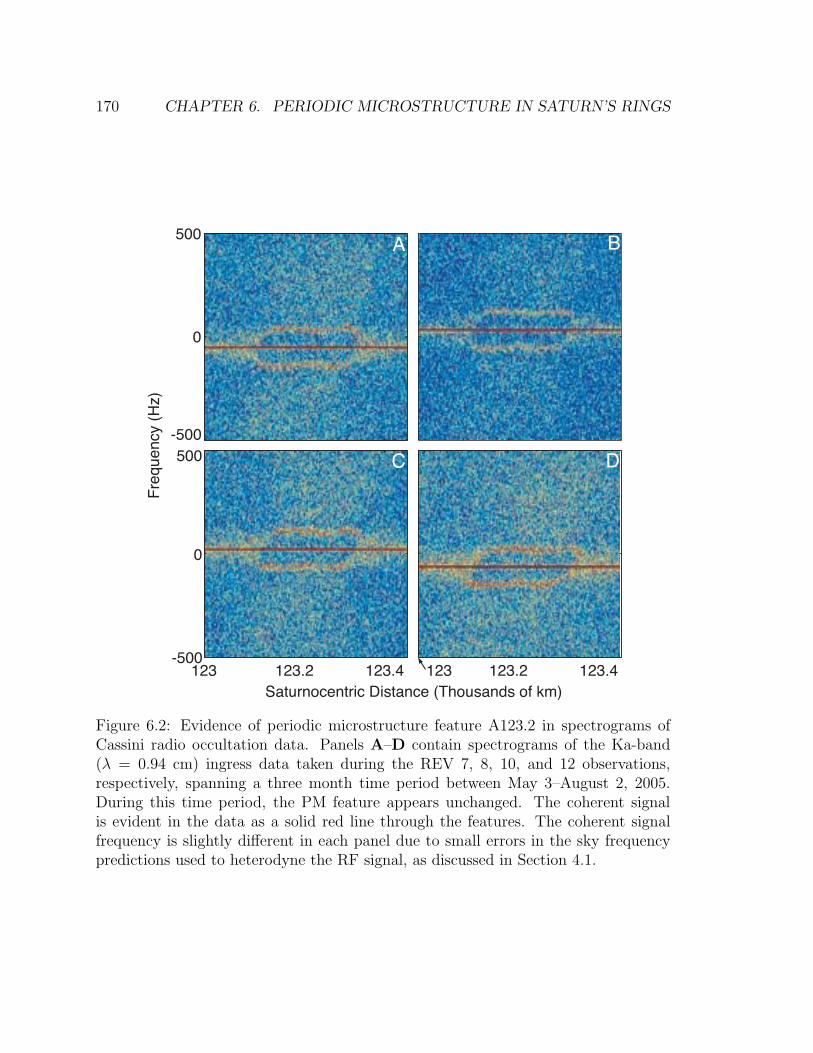
170 CHAPTER 6. PERIODIC MICROSTRUCTURE IN SATURN’S RINGS
Fre
quen
cy (
Hz)
-500
0
500
Saturnocentric Distance (Thousands of km)123 123.2 123.4 123 123.2 123.4
-500
0
500
A
C
B
D
Figure 6.2: Evidence of periodic microstructure feature A123.2 in spectrograms ofCassini radio occultation data. Panels A–D contain spectrograms of the Ka-band(λ = 0.94 cm) ingress data taken during the REV 7, 8, 10, and 12 observations,respectively, spanning a three month time period between May 3–August 2, 2005.During this time period, the PM feature appears unchanged. The coherent signalis evident in the data as a solid red line through the features. The coherent signalfrequency is slightly different in each panel due to small errors in the sky frequencypredictions used to heterodyne the RF signal, as discussed in Section 4.1.

6.1. A SURVEY OF PM IN SATURN’S RINGS 171
Saturnocentric Distance (Thousands of km)122.5 123 123.5 124 124.5
Fre
quen
cy (
Hz)
-500
0
500
-500
0
500
-500
0
500
5
10
15
dB R
elat
ive
to N
oise
Flo
or
0
5
10
15
20
A
C
B
Figure 6.3: PM features A123.2 and 124.1 are seen in spectrograms of Cassini S-, X-,and Ka-band (λ= 13, 3.6, and 0.94 cm, respectively) radio occultation data, shownin panels A–C, respectively. The slanting of the feature in the frequency domain isa function of the wavelength of the observation, as described in Section 4.1.2. Thehigher SNR of the X- and Ka-band signals is evident in the brightness of the featuresand the color scaling, relative to the S-band data.

172 CHAPTER 6. PERIODIC MICROSTRUCTURE IN SATURN’S RINGS
-1 0 1-30
-20
-10
0
Frequency (kHz)
Inte
nsity
(dB
)
-1 0 1
-20
-15
-10
-5
0
-1 0 1 -1 0 1 -1 0 1Frequency (kHz)
A B
D EC
Figure 6.4: Power spectra of periodic microstructure features in Saturn’s rings. PanelsA–E are produced using 3.6 cm-λ (X–band) radio occultation data recorded duringthe Cassini REV 7 ingress observation of the rings. Panel A shows the received signalspectrum of feature A123.2., averaged over the radial range 123.1–123.35×10³ km.Similarly, panels B–E show the spectra of features A124.1 and B92.4, and regionsB2 and B4, respectively. The radial range of the signal averaging in panels B–Eis 123.9–124.5×10³ km, 92.28–92.5×10³ km, 99–104×103 km, and 110–116×103 km,respectively. In each panel, the signal intensity is plotted in decibels relative tothe average coherent signal intensity over the extent of each particular feature. Alldistances are given with respect to Saturn’s geometric center. Compare with Figures4.5, 5.10, 6.1–6.3; see the text for a more detailed discussion.

6.2. ESTIMATES OF PHYSICAL PARAMETERS λGR AND φGR 173
6.2 Estimates of Physical Parameters λgr and φgr
The results we present in this chapter derive from our analysis of REV 7, 8, 10, and 12
ingress and egress observations, which occurred between May 3 and August 2, 2005.
These observations were optimized for the experiment, as described in Chapter 4.
For features A123.2 and A124.1 (Fig. 6.1), we estimate λgr, φgr in approximately
25-km radial steps across the features. Within each step, a series of spectral slices
of the received signal are non-coherently averaged to reduce noise and sharpen the
diffraction lobes, facilitating cleaner Gaussian fits. The procedure is applied to both
the 0.94 cm- and the 3.6 cm-λ measurements from each of the eight ring observations.
We apply the diffraction grating modeling approach described in Chapter 5 to
obtain estimates of the PM features identified in Section 6.1. We present our estimates
of λgr and φgr for ring features A123.2, A124.1, and B2 in Figure 6.5. The figure is
presented in four parts, (a)–(d), and each part contains four panels, A–D. Part (a)
and (b) contain estimates of λgr and φgr, respectively, computed using the diffraction
grating model explained in Section 5.2.2. Parts (c) and (d) depict estimates of λgr
and φgr that we compute using the sinusoidal transmittance screen model described
in Section 5.2.1. In all parts (a)–(d), panels A and B correspond to features A123.2
and A124.1, respectively, and panels C and D correspond to two sub-regions of B2,
which we discuss in more detail below. Each panel of Figure 6.5 contains parameter
estimates we obtained by processing the Ka-band data, shown in blue; blue dots
represent point estimates of either λgr or φgr; a blue shaded region represents the
uncertainty bounds on the estimate, computed from fσ1−, fσ1+, fσ2−, and fσ2+ as
explained in Section 5.4. Similarly, red dots and shaded regions correspond to the
estimates we produced using X-band data. Purple regions mark the overlap of blue
and red regions. The mean values λgr and φgr are shown as dashed lines in the figure.
Estimates of λgr for features A123.2 and A124.1 are presented in Figure 6.5(a)
panels A and B, respectively. Across the ‘flattest’ part of feature A123.2, λgr varies
between 140–160 meters. Near the edge of A123.2, the structural period λgr sharply
increases; this does not appear to be a general characteristic of PM feature boundaries,
cf. panels B–D of Figure 6.5. Averaging the λgr estimates across all of A123.2 yields

174 CHAPTER 6. PERIODIC MICROSTRUCTURE IN SATURN’S RINGS
an average structural period λgr = 163+−6 meters, where the bound on the average
is the standard deviation of the fluctuations in the estimates across the feature. For
feature A124.1, λgr varies between 180–250 meters with an average λgr = 217+−8
meters. Possible systemic deviation from the mean estimate is evident in Figure
6.5(a), panel B.
Colored regions in Fig. 6.5 characterize the deviations from the local estimates λgr
and φgr due to Doppler spreading of the observed spectral features around the mean
frequency. As evident, the deviations for A124.1 are larger than for A123.2. Spectral
spreading of the first-order diffraction lobe frequencies seen in A124.1, combined with
a general increase in the background scattered signal level in A124.1 as compared
with A123.2, leads to estimates of fmi with larger standard deviation. For A123.2, the
0.94 cm-λ estimates were better constrained than the 3.6 cm-λ estimates, primarily
because of the weaker background scattered signal at 0.94 cm-λ.
In presenting the estimates of λgr and φgr for region B2, we have removed the large
optical depth feature between 100.0–101.1 × 10³ km (see Figure 6.1, panel F), thus
splitting B2 into two sub-regions as shown in Figure 6.5, panels C and D. In general,
estimates of λgr within B2 vary between 100–200 meters, with λgr = 146+−14 meters.
Spectral averages for B2 were computed over approximately 100 km-wide bands to
mitigate noise. The spread in the B2 estimates is better-constrained than the Ring
A results for two reasons. First, we are averaging over 100-km as opposed to 25-km.
Second, because the background scattered signal is much weaker in B2 than in Ring
A, the grating lobes peaks appear more distinct, enhancing the ability to estimate
fmi.
For the relatively optically thick (τ > 2) feature B92.4 and region B4, the mea-
sured grating lobes appear less spectrally confined compared with region B2 and Ring
A features. Because of SNR limitations, we only use 3.6 cm-λ data in our estimates.
For B92.4, we estimate fmi from one spectral average over most of its radial extent
of a 500-km band between 92.1–92.6 × 10³ km. The feature-wide average λgr is ap-
proximately 115+20−15 meters. For B4, we spectrally averaged a 5000-km swath from
110.0–115.0× 10³ km, yielding λgr ≈ 250+150−75 meters.
Results for all regions studied show that the data is best fit with diffraction grating
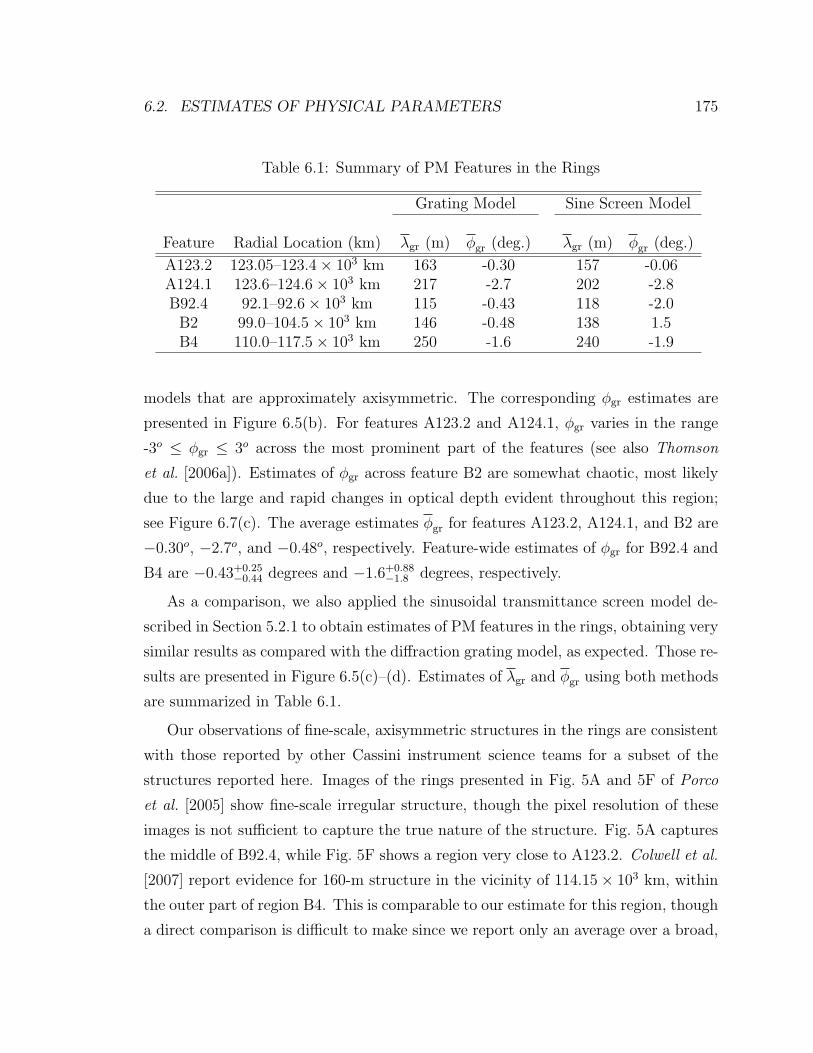
6.2. ESTIMATES OF PHYSICAL PARAMETERS 175
Table 6.1: Summary of PM Features in the Rings
Grating Model Sine Screen Model
Feature Radial Location (km) λgr (m) φgr (deg.) λgr (m) φgr (deg.)
A123.2 123.05–123.4× 10³ km 163 -0.30 157 -0.06A124.1 123.6–124.6× 10³ km 217 -2.7 202 -2.8B92.4 92.1–92.6× 10³ km 115 -0.43 118 -2.0B2 99.0–104.5× 10³ km 146 -0.48 138 1.5B4 110.0–117.5× 10³ km 250 -1.6 240 -1.9
models that are approximately axisymmetric. The corresponding φgr estimates are
presented in Figure 6.5(b). For features A123.2 and A124.1, φgr varies in the range
-3o ≤ φgr ≤ 3o across the most prominent part of the features (see also Thomson
et al. [2006a]). Estimates of φgr across feature B2 are somewhat chaotic, most likely
due to the large and rapid changes in optical depth evident throughout this region;
see Figure 6.7(c). The average estimates φgr for features A123.2, A124.1, and B2 are
−0.30o, −2.7o, and −0.48o, respectively. Feature-wide estimates of φgr for B92.4 and
B4 are −0.43+0.25−0.44 degrees and −1.6+0.88
−1.8 degrees, respectively.
As a comparison, we also applied the sinusoidal transmittance screen model de-
scribed in Section 5.2.1 to obtain estimates of PM features in the rings, obtaining very
similar results as compared with the diffraction grating model, as expected. Those re-
sults are presented in Figure 6.5(c)–(d). Estimates of λgr and φgr using both methods
are summarized in Table 6.1.
Our observations of fine-scale, axisymmetric structures in the rings are consistent
with those reported by other Cassini instrument science teams for a subset of the
structures reported here. Images of the rings presented in Fig. 5A and 5F of Porco
et al. [2005] show fine-scale irregular structure, though the pixel resolution of these
images is not sufficient to capture the true nature of the structure. Fig. 5A captures
the middle of B92.4, while Fig. 5F shows a region very close to A123.2. Colwell et al.
[2007] report evidence for 160-m structure in the vicinity of 114.15× 10³ km, within
the outer part of region B4. This is comparable to our estimate for this region, though
a direct comparison is difficult to make since we report only an average over a broad,

176 CHAPTER 6. PERIODIC MICROSTRUCTURE IN SATURN’S RINGS
5000 km swath between ro = 110× 103 km and ro = 115× 103 km.

6.2. ESTIMATES OF PHYSICAL PARAMETERS 177
Next four pages.
Figure 6.5: Estimates of the structural period λgr and orientation φgr of periodicmicrostructure detected in Saturn’s rings. Estimates of λgr and φgr produced using adiffraction grating model are shown in Figures (a) and (b), respectively; Figures (c)and (d) show estimates of λgr and φgr produced with a sinusoidal transmittance screenmodel. In each of Figures (a)–(d), panels A and B detail features A123.2, A124.1,while C and D show region B2. Estimates in red are 3.6 cm-λ data, estimates inblue are 0.94 cm-λ data. The red and blue shaded regions correspond to the spreadin λgr computed based on the 1-σ width of Gaussian functions fitted to the observedspectral features in the 3.6 and 0.94 cm-λ observations, respectively. Light purple isshown where the red and blue regions overlap. The dashed lines represent the averageof the estimates, λgr and φgr, across a given region.

178 CHAPTER 6. PERIODIC MICROSTRUCTURE IN SATURN’S RINGS
123.8 123.9 124 124.1 124.2 124.3 124.4
Saturnocentric Distance (Thousands of km)
101 101.5 102 102.5 103 103.5
123.2 123.3
99.5 100
0
50
100
150
200
250
300
350
400
Str
uctu
ral P
erio
d λ
gr (
met
ers)
0
50
100
150
200
250
300
350
400
λgr = 217 meters
λgr = 146 meters
λgr = 163 meters
A
DC
B
(a) Estimates of the structural period λgr using a diffraction grating model.

6.2. ESTIMATES OF PHYSICAL PARAMETERS 179
123.8 123.9 124 124.1 124.2 124.3 124.4
Saturnocentric Distance (Thousands of km)
101 101.5 102 102.5 103 103.5
123.2 123.3
99.5 100-25
-20
-15
-10
-5
0
5
10
15
20
25
Str
uctu
ral O
rient
atio
n φ
gr (
degr
ees)
-25
-20
-15
-10
-5
0
5
10
15
20
25
φgr = -0.48o
φgr = -2.7o
φgr = -0.30o
A
DC
B
(b) Estimates of the structural orientation φgr using a diffraction grating model.

180 CHAPTER 6. PERIODIC MICROSTRUCTURE IN SATURN’S RINGS
123.8 123.9 124 124.1 124.2 124.3 124.4
Saturnocentric Distance (Thousands of km)
101 101.5 102 102.5 103 103.5
123.2 123.3
99.5 100
0
50
100
150
200
250
300
350
400
Str
uctu
ral P
erio
d λ
gr (
met
ers)
0
50
100
150
200
250
300
350
400
λgr = 202 meters
λgr = 138 meters
λgr = 157 meters
A
DC
B
(c) Estimates of the structural period λgr using a sinusoidal amplitude screen model.

6.2. ESTIMATES OF PHYSICAL PARAMETERS 181
123.8 123.9 124 124.1 124.2 124.3 124.4
Saturnocentric Distance (Thousands of km)
101 101.5 102 102.5 103 103.5
123.2 123.3
99.5 100-25
-20
-15
-10
-5
0
5
10
15
20
25
Str
uctu
ral O
rient
atio
n φ
gr (
degr
ees)
-25
-20
-15
-10
-5
0
5
10
15
20
25
φgr = -2.8o
φgr = -0.06o
φgr = 1.5o
A
DC
B
(d) Estimates of the structural orientation φgr using a sinusoidal amplitude screenmodel.

182 CHAPTER 6. PERIODIC MICROSTRUCTURE IN SATURN’S RINGS
Next page.
Figure 6.6: Fine-scale optical depth variation τfs within features in Ring A is shownusing REV 7 ingress data. Feature A123.2 estimates are shown in panels A and C;feature A124.1 estimates are shown in panels B and D. Ka- and X- band data areshown in blue and red, respectively. Estimates of the normal optical depth τ retrievedby analysis of the coherent signal are shown as solid lines in the plots. The fine-scaleoptical depth variation τfs is indicated by the shaded area.

6.2. ESTIMATES OF PHYSICAL PARAMETERS 183
Nor
mal
Opt
ical
Dep
th τ
0.7
0.8
0.9
1
1.1
1.2
1.3
1.4
1.5
1.6
1.7
Saturnocentric Distance (Thousands of km)
123.9 124 124.1 124.2 124.3 124.4123.2 123.3
0.7
0.8
0.9
1
1.1
1.2
1.3
1.4
1.5
1.6
1.7
A
DC
B

184 CHAPTER 6. PERIODIC MICROSTRUCTURE IN SATURN’S RINGS
6.3 Optical Depth Variation within Features A123.2
and A124.1
In Ring A, PM features exhibit first-order diffraction lobes that are 5–10 dB above the
background scattered signal, as shown in Figures 4.5 and 5.13. Taking advantage of
the high SNR in this region, we applied the theory of Section 5.2.1, eqs. (5.2)–(5.5),
to estimate the fine-scale variation in optical depth τfs that exists within features
A123.2 and A124.1. The results are presented in Figure 6.6, which shows that τ
varies by approximately ±0.3 within the two features. Estimates we calculated using
both Ka-band and X-band data produced consistent results for τfs,min and τfs,max.
6.4 Discussion
The origins of periodic microstructure in the rings is a subject of ongoing debate
and research. At present, a phenomenon known as viscous or pulsation overstability
is the leading dynamical theory to explain the existence of PM in Saturn’s rings
(e.g., Cuzzi et al. [2002]). In this section we discuss the threshold conditions for the
onset of viscous overstability (VO) in the rings, and compare those conditions with
our observations to determine whether the VO threshold criteria explains the limited
regions where PM is detected. We also present and discuss evidence in our data
that may possibly indicate regions of Ring B where PM is superimposed on other
microstructure.
6.4.1 Concurrent Microstructure
Salo et al. [2001] report that axisymmetric periodic structure due to viscous over-
stability co-exists with gravitational wakes in dynamical simulations, as long as the
wakes are not too prominent. This coexistence is not predicted by any known analytic
theory [Schmidt et al., 2009].
Evidence for the existence of gravitational wakes is clearly present in the radio
occultation data in both Rings A and B [Marouf et al., 2006a]. The broad presence

6.4. DISCUSSION 185
of gravitational wakes across Rings A and B has been observed in back-scattered and
UBVRI-filtered optical images of the rings taken using the Hubble Space Telescope
(HST) [French et al., 2007], and at radiometric wavelengths using the Very Large
Array (VLA) [Dunn et al., 2007].
There is evidence contained in our scattered signal observations that hints at a
superposition of PM with other microstructure. In panels C–D of Figure 6.4, we
see varying degrees of a double-humped structure in the forward scattering lobe—in
addition to the distinct sidelobes associated with PM—that may indicate the presence
of gravitational wakes, or possibly a packed monolayer of large particles (cf. Figure
5.1). Using the received signal synthesis technique explained in Chapter 5, we have
been unable to produce a synthesized spectrum I(fD) from packed monolayer models
that contains these double-humped features (Figure 5.10). However, we have not
performed a thorough investigation of the packed monolayer model parameter space,
and thus we are unable to rule out monolayers as a possible cause of humps in the
signal spectrum. In panel E the narrow forward-scattering pattern, as compared with
that of all the other panels in the figure, as well as the small region of enhancement in
very near forward-scattering that is visible very close (in frequency) to the coherent
signal may indicate the presence of gravitational wakes in combination with larger
particle sizes (on average). This conjecture is unproved, and we leave the analysis of
this phenomenon as a suggestion for future work.
6.4.2 The Onset of Viscous Overstability
In dynamical studies of dense rings, viscous overstability is accompanied by the for-
mation of axisymmetric structures with small-scale periodicity on the order of one
to few hundreds of meters [Schmit and Tscharnuter , 1999; Salo et al., 2001; Schmidt
et al., 2001; Salo and Schmidt , 2009]. Recent theoretical studies by Latter and Ogilvie
[2008, 2009] investigate the onset of viscous overstability (VO) using dense kinetic gas
theory to model the rings, and propose that nonlinear wavetrains arising naturally
in a viscously overstable disk can explain the presence of axisymmetric periodic mi-
crostructure.

186 CHAPTER 6. PERIODIC MICROSTRUCTURE IN SATURN’S RINGS
Planetary rings become overstable if the extent to which viscosity increases with
optical depth exceeds a certain rate (e.g., Schmidt et al. [2009]). Latter and Ogilvie
[2008] conclude that regions of overstability are possible anywhere in the rings, as
long as a threshold optical depth τth is exceeded, although they also conclude that
the filling factor—not τ , explicitly—is the parameter that determines the onset of VO.
In both theoretical and dynamical studies, models of the rings predict a threshold
optical depth on the order of τth ∼ 1.
Other than τth, specific estimates of the physical conditions that produce viscously
overstable regions vary. Schmit and Tscharnuter [1995] say that VO onset occurs
when,
β =d[ln νσρ]
d[ln σρ]≥ sufficiently large (6.1)
where ν is the kinematic shear viscosity, and σρ is the surface mass density of the
rings. Salo et al. [2001] interpret the results of Schmit and Tscharnuter [1995] to
yield the following VO onset condition,
β =dν
dτ
(τν
)> βcr =
1
9(6.2)
This is inconsistent with dynamical simulation results generated by Schmidt et al.
[2001], who propose a different VO onset condition,
β =d[ln ν]
d[ln σρ]≥ βcr = 1 (6.3)
which is derived from hydrodynamic theory and is consistent with dynamical simu-
lation results [Schmidt et al., 2001]. This appears now to be a generally agreed-upon
threshold condition [Schmidt et al., 2009].
Several forms exist in the literature for computing ν. Colwell et al. [2009] report
that,
ν = k1c2
Ω
τ
τ 2 + 1+ 4k2Ωτa
2 (6.4)
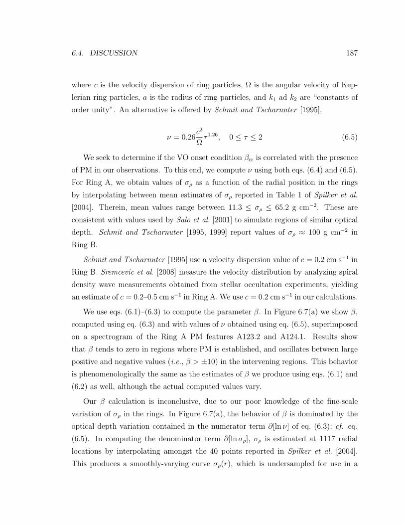
6.4. DISCUSSION 187
where c is the velocity dispersion of ring particles, Ω is the angular velocity of Kep-
lerian ring particles, a is the radius of ring particles, and k1 ad k2 are “constants of
order unity”. An alternative is offered by Schmit and Tscharnuter [1995],
ν = 0.26c2
Ωτ 1.26, 0 ≤ τ ≤ 2 (6.5)
We seek to determine if the VO onset condition βcr is correlated with the presence
of PM in our observations. To this end, we compute ν using both eqs. (6.4) and (6.5).
For Ring A, we obtain values of σρ as a function of the radial position in the rings
by interpolating between mean estimates of σρ reported in Table 1 of Spilker et al.
[2004]. Therein, mean values range between 11.3 ≤ σρ ≤ 65.2 g cm−2. These are
consistent with values used by Salo et al. [2001] to simulate regions of similar optical
depth. Schmit and Tscharnuter [1995, 1999] report values of σρ ≈ 100 g cm−2 in
Ring B.
Schmit and Tscharnuter [1995] use a velocity dispersion value of c = 0.2 cm s−1 in
Ring B. Sremcevic et al. [2008] measure the velocity distribution by analyzing spiral
density wave measurements obtained from stellar occultation experiments, yielding
an estimate of c = 0.2–0.5 cm s−1 in Ring A. We use c = 0.2 cm s−1 in our calculations.
We use eqs. (6.1)–(6.3) to compute the parameter β. In Figure 6.7(a) we show β,
computed using eq. (6.3) and with values of ν obtained using eq. (6.5), superimposed
on a spectrogram of the Ring A PM features A123.2 and A124.1. Results show
that β tends to zero in regions where PM is established, and oscillates between large
positive and negative values (i.e., β > ±10) in the intervening regions. This behavior
is phenomenologically the same as the estimates of β we produce using eqs. (6.1) and
(6.2) as well, although the actual computed values vary.
Our β calculation is inconclusive, due to our poor knowledge of the fine-scale
variation of σρ in the rings. In Figure 6.7(a), the behavior of β is dominated by the
optical depth variation contained in the numerator term ∂[ln ν] of eq. (6.3); cf. eq.
(6.5). In computing the denominator term ∂[ln σρ], σρ is estimated at 1117 radial
locations by interpolating amongst the 40 points reported in Spilker et al. [2004].
This produces a smoothly-varying curve σρ(r), which is undersampled for use in a

188 CHAPTER 6. PERIODIC MICROSTRUCTURE IN SATURN’S RINGS
rate-of-change calculation.
We could not compute β in Ring B, since we do not have an estimate of σρ(r)
in that region (recall we have only a single value, σρ ≈ 100 g cm−2). Plots of the
numerator ∂[ln ν] alone over radial regions bounding feature B92.4, and regions B2
and B4, yielded results that are also inconclusive.
In summary, better estimates of σρ(r) are needed in order to compute meaningful
estimates of β.
6.4.3 Optical Depth Characteristics of PM Regions
Although our calculations of the VO onset condition β ≥ βcr are not conclusive, a pre-
liminary assessment of the correlation between measured optical depth characteristics
and the presence of PM yields more promising results. Here, we focus our attention
on Ring A and feature B92.4, since the highly oscillatory nature of the optical depth
in regions B2 and B4, combined with the large observed optical depth, renders any
conclusions drawn from our observations in those regions more uncertain.
Optical depth observations suggest that regions of PM are bounded by sharp
transitions in ring optical depth, combined with the condition that the normal optical
depth τ > 1. In Ring A, relatively sharp transitions in optical depth on the order of
∆τ > 0.3 appear to bound PM feature A123.2 on either side, and feature A124.1 on
the low side (i.e., on the side closest to Saturn); see Figure 6.7(a). On its upper side
(i.e., r ≈124,500 km), feature A124.1 appears to dissipate as the local optical depth
decreases below τ ≈ 1. This is consistent with the predictions of hydrodynamical
theory and with the results of dynamical simulations, as discussed in Section 6.4.2.
In feature B92.4, we see similar behavior—the region containing PM is bounded
by sharp transitions in optical depth, where ∆τ > 0.3 on both sides of the feature.
This is evident in Figure 6.7(b).
The same is true of regions B2 and B4. However, the optical depth in these regions
exceeds the measurement capability of the radio instrument in many places, making
it impossible to determine whether PM features exist continuously across B2 and B4,
or whether the sharp transitions in optical depth—to values of τ that completely

6.4. DISCUSSION 189
Next two pages.
Figure 6.7: Optical depth and spectrogram plots of periodic microstructure featuresobserved during the REV 7 ingress occultation. In each plot, the top panel shows theoptical depth at 13, 3.6, and 0.94 cm wavelengths (S-, X, and Ka-band, respectively).The spectrograms are produced from the X-band (λ = 3.6 cm) received signal. Shownare (a) features A123.2 and A124.1; (b) feature B92.4; (c) the B2 region; and (d) theB4 region. In (a), we overlay the computed value of the dynamical parameter β (seeeq. (6.3)) on the spectrogram plot. According to Schmidt et al. [2009], the onset ofviscous overstability occurs when β ≥ 1. Our calculations are not conclusive on thispoint. See the text for a more detailed discussion.

190 CHAPTER 6. PERIODIC MICROSTRUCTURE IN SATURN’S RINGS
0
0.5
1
1.5
2
2.5
Nor
mal
Opt
ical
Dep
th τ
Saturnocentric Distance (Thousands of km)122.5 123 123.5 124 124.5
S-bandX-bandKa-band
Fre
quen
cy (
Hz)
-500
0
500
-200
0
200
∂[ln
ν]
∂[ln
σ]
β =
(a) Normal optical depth and spectrogram of features A123.2 and A124.1. The pa-rameter β is superimposed (in black) on the spectrogram, with scale provided at theright of the figure. See Figure 6.3 for a clean spectrogram of these features.
0
1
2
3
Nor
mal
Opt
ical
Dep
th τ
Saturnocentric Distance (Thousands of km)91.5 92 92.5 93
S-bandX-bandKa-band
Fre
quen
cy (
Hz)
-500
0
500
(b) Normal optical depth and spectrogram of feature B92.4.
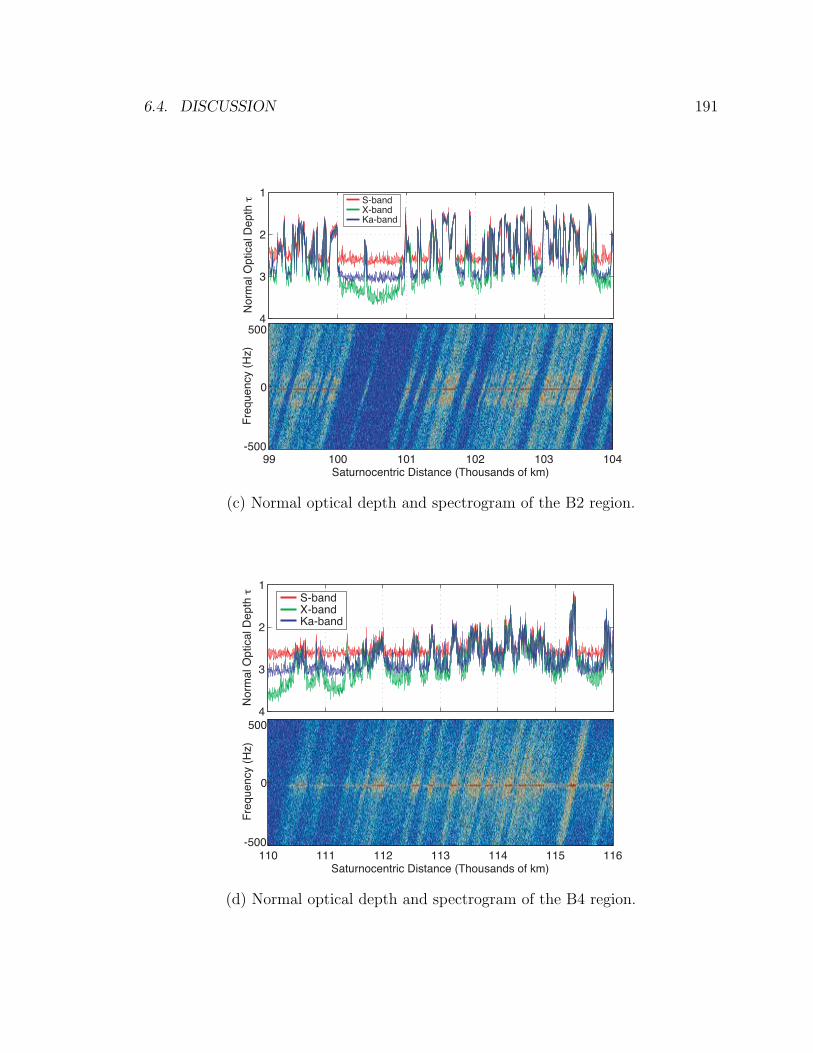
6.4. DISCUSSION 191
1
2
3
4
Nor
mal
Opt
ical
Dep
th τ
Saturnocentric Distance (Thousands of km)99 100 101 102 103 104
S-bandX-bandKa-band
Fre
quen
cy (
Hz)
-500
0
500
(c) Normal optical depth and spectrogram of the B2 region.
1
2
3
4
Nor
mal
Opt
ical
Dep
th τ
S-bandX-bandKa-band
Saturnocentric Distance (Thousands of km)110 111 112 113 114 115 116
Fre
quen
cy (
Hz)
-500
0
500
(d) Normal optical depth and spectrogram of the B4 region.

192 CHAPTER 6. PERIODIC MICROSTRUCTURE IN SATURN’S RINGS
extinguish the radio signals—actually bound regions containing PM.
It is foolish to mistake correlation with causation, and we do not make that mistake
here. Our intent is to make a preliminary report of our observations regarding τ and
the presence of PM. A definitive cause of PM in Saturn’s rings remains to be proved;
that task is beyond the scope of this dissertation.
6.5 Summary
We have uncovered and reported on five distinct instances of periodic microstructure
in Saturn’s Ring A and B. The mean structural period λgr of the PM we observe
varies between 115–250 meters. We determine that all PM regions are approximately
axisymmetric, with mean estimates of the orientation (using both the grating and
sinusoidal screen methods) ranging between −2.8o ≤ φgr ≤ 1.5o. The results of these
investigations are reported formally in Thomson et al. [2007].
Axisymmetric structure with small-scale periodicity on the order of hundreds of
meters is predicted by both hydrodynamic theory, and by dynamical simulations of the
rings. These structures appear in regions of the rings that exhibit a phenomenology
known as viscous overstability (VO), the onset of which is controlled by a parameter
β, and by the condition that τ > 1.
We observe the termination of feature A124.1 at approximately r =124,500 km
when the optical depth τ decreases below τ ≈ 1, which is consistent with theory
[Latter and Ogilvie, 2008; Schmidt et al., 2009]. Elsewhere, we observe the termination
of PM features when relatively large changes in optical depth, ∆τ > 0.3 or so, occur.
Theory and dynamical simulation results predict that regions where the shear
viscosity is increasing much faster than the optical depth mark the onset of viscously
overstable regions. Measures of this are formalized by the parameter β, versions of
which are presented in eqs. (6.1)–(6.3). We are unable to effectively compute β in
the rings due to the poor spatial resolution of our surface mass density σρ estimates
in regions of the rings where PM exists. Thus we cannot conclusively state whether
or not the conditions for VO have been strictly met in the regions where we have
observed PM. We leave this as an open question for future researchers to answer.

6.5. SUMMARY 193

194 CHAPTER 6. PERIODIC MICROSTRUCTURE IN SATURN’S RINGS

Chapter 7
Summary and Conclusions
In this chapter we summarize the findings of our work, and its relevance in the context
of the pre-Cassini understanding of Saturn’s rings. This is followed by a discussion
of the assumptions and limitations inherent to our model, and the associated impli-
cations for our results. Suggestions for future work are discussed in the final section.
7.1 General Results
The methods that we have developed for estimating the dimensions of microstructure
in Saturn’s rings rely on our ability to apply scalar diffraction theory to the analysis
of forward scattering from ring microstructure. We have proved that the assumptions
of scalar diffraction theory are satisfied by the conditions of the radio occultation
experiments. Specifically, we showed that as long as the ring particles are electrically
large, and as long as we are measuring radio signals in the near-forward scattering
direction, then scalar diffraction theory produces estimates of the scattering pattern
that closely mimic those produced using full electromagnetic theory. Both of these
conditions are met by the experiment. Our detailed analysis is shown in Chapter 3
and also in Thomson and Marouf [2009].
We have shown that axisymmetric periodic microstructure with length scales vary-
ing between 100–250 meters exists in (at least) five distinct regions within Saturn’s
195

196 CHAPTER 7. SUMMARY AND CONCLUSIONS
rings. We uncovered two distinct features in Ring A at radial locations 123.05–
123.4×10³ km and 123.6–124.6×10³ km, which we have named A123.2 and A124.1,
respectively. These features have mean structural periods ranging between 160–220
meters. At a radial location spanning 92.1–92.6×10³ km in Ring B, feature B92.4 is
detectible with an estimated mean structural period of 115 meters. PM structure is
seen in two broad regions of Ring B known as B2 and B4, located at 99–104.5×10³
km and 110–117.5×10³ km, respectively. Here, we estimate mean structural periods
of 146 meters and 250 meters, respectively. These details are summarized in Chapter
6 (see Table 6.1). The results are also reported in Thomson et al. [2007].
Prior to Cassini, the existence of axisymmetric periodic microstructure had been
predicted by dynamicists investigating the properties of planetary rings. Some scien-
tists had applied dynamical theory specifically to Saturn’s Ring B, which was known
(after Voyager) to contain regions of sharply oscillating optical depth. However, no
measurements of ring optical depth existed on length scales that could detect PM
features with wavelengths on the order of 100 meters, which was the value of λgr
predicted by dynamicists.
Our results were among the first direct observations of these features in the rings.
We had the good fortune to be in the right place at the right time—and with the
right instrument—to validate the predictions of the dynamical theory.
7.2 Assumptions and Limitations
Several assumptions were incorporated in the development of our methods. First, we
have assumed in our analysis that features contained in the rings do not change during
the period of our observations, which spanned the dates May 3–August 2, 2005. The
observations we made during this period were used together to produce estimates of
the dimensions of detected periodic microstructure. We believe that this is a reason-
able assumption, since we do not detect any evidence that the either the location of
the features, or the physical dimensions of the features changed significantly during
that three-month period. This is not surprising, since the collisional and gravitational
forces that create these features are not changing on short time scales. It is possible

7.2. ASSUMPTIONS AND LIMITATIONS 197
that inter-particle collisions could break larger ring particles apart over time, driving
an evolution in the particle size distributions local to a PM feature that could perhaps
change the dimensions of the feature in some measurable way. However, we believe
that those mechanisms take place on time scales that are longer than the 3-month
period of the observations we use in our analysis, although that point is not proved.
In fitting our PM models to the data, we assume a sinusoidal variation in optical
depth. The optical depth variation of PM regions in the rings, caused by VO and
predicted by hydrodynamic theory and dynamical simulations, are not purely sinu-
soidal. Theory predicts a nonlinear periodic structure, and thus diffraction from PM
should produce higher order sidelobes in the received signal. The best-case SNR we
achieved with first-order sidelobe measurements was on the order of 5–10 dBn (the
3.6 cm-λ measurements of feature A123.2); higher order diffraction lobes were not
detected within this 5–10 dB detection limit. From this, we surmise that most of the
diffracted signal power is contained in the first-order lobes, and that our estimates of
structural period and orientation should be correct, even if the precise variation of
optical depth within a period of the structure remains unknown.
Another limitation in our method is caused by the slanting of features in our
spectrograms, as explained in Section 4.1.2. Currently, our sidelobe peak estimation
algorithm, eq. (5.20), fits a Gaussian function to the diffraction sidelobes at each
step in |ro| without de-slanting the spectrogram to remove the effect of the finite
HGA spot size. Thus, we incur errors in our estimates of the physical dimensions of
PM. Because of its greater slant angle, the X-band data is more vulnerable to this
error than is Ka-band. The errors are greatest in parts of a PM feature where the
physical dimensions are changing—at either end of feature A123.2, for example. In
the middle of a feature, the Doppler frequencies associated with PM are relatively
constant, which lessens the estimation error. Averaging over broader swaths in the
rings also reduces the error, but yields a coarser spatial resolution of our λgr and
φgr estimates. The limitation due to spectral slanting represents the most significant
weakness in our model.

198 CHAPTER 7. SUMMARY AND CONCLUSIONS
7.3 Contributions
As we have stated in Section 1.3, the major contributions of this work are as follows:
1. We uncovered five distinct locations in Saturn’s rings A and B exhibiting highly
periodic, fine-scale variation in the ring optical depth. The physical period of
these variations range between 100–250 meters [Thomson et al., 2007].
2. An exhaustive study, comparing the results of a multiple scattering formulation
of Mie theory against the results of scalar diffraction theory. The study, which
examined 2-, 3-, and 10-sphere clusters of particles, shows that diffraction theory
accurately predicts the far-field scattering pattern of particle aggregates, as long
as the region of interest is limited to electrically large particles scattering in the
near-forward direction [Thomson and Marouf , 2009].
3. Derivation of the exact solution for the five-term power-law expression of Al-
lan variance, showing that the exact solution and the well-known approximate
solution converge very quickly; i.e., the approximate form is sufficient and sat-
isfied by most imaginable measurement conditions [Thomson et al., 2005]. An
adaptation of this paper is included as Appendix D.
4. Demonstration of the equivalence of the Radon and Abel Transforms, as they
are applied in atmospheric radio occultation [Thomson and Tyler , 2007]. An
adaptation of this paper is included as Appendix E.
7.4 Future Work
Prior to Cassini, the only radio occultation data available for Saturn’s rings were
gathered during the Voyager 1 flyby of Saturn on November 13, 1980; a single egress
pass lasting approximately 1000 seconds, with a ring opening angle of B ≈ 6o.
Cassini has produced multiple radio occultation datasets, sampled during obser-
vations that span a range of ring opening angles between 0 ≤ B ≤ 23.6, and over
many ring longitudes. With multiple experimental observations—at radio and other

7.4. FUTURE WORK 199
wavelengths—of the same ring system now available, the time evolution of rings can
be studied. The azimuthal asymmetry of Saturnian ring optical depth, thought to be
produced by canted gravitational wakes [Salo, 1992; Salo et al., 2004], can be mea-
sured by comparing occultation tracks at different Saturnian longitudes. Analysis
of the effect of changing observational parameters, such as ring opening angle and
longitude, add a new dimension to data reduction that is certain to result in a more
complete picture of the structure and dynamics of the rings, and how they evolve
over time.
There are many opportunities for improvement, extension, or application of the
methods developed in this dissertation. On the signal processing side, more advanced
peak detection methods could be used to produce better Gaussian (or other) fits to
features of the received signal, improving the input to our estimation codes. Advanced
estimation methods, such as Kalman filtering, could be applied to use different kinds
of data together to produce better estimates of physical microstructure dimensions.
Advanced signal processing methods could also be used to determine definitively the
sensitivity of the measurement to the presence of higher-order diffraction lobes in the
received signal, and to verify with greater confidence that they are not hidden in our
received signal.
Theoretical studies that determine the uniqueness of scattering from homogeneous
rings, monolayers, clumped ring models, gravitational wakes, and periodic microstruc-
ture can be performed by using the amplitude screen method in combination with
statistical methods. The findings of such a study could help guide the use of different
microstructure models in cases where diffraction features contained in the scattered
signal are more subtle, and therefore determining the underlying microstructure is
more challenging.
Collaborative partnerships with ring dynamicists could yield estimates of many
underlying physical properties of the rings that that best-fit regions of the rings con-
taining detected microstructure. In this scenario, dynamical simulations are used to
generate vignettes of the rings that contain microstructure. The underlying physi-
cal properties—such as surface mass density, ring thickness, etc.—are varied in the
optimization that fits synthesized spectral features to those detected in the Cassini

200 CHAPTER 7. SUMMARY AND CONCLUSIONS
received signal.
Figure 7.1: This panoramic view of the unlit side of Saturn and the rings is a compositeof 165 images taken by the Cassini wide-angle camera during approximately threehours on Sept. 15, 2006. Colors in the mosaic were created by digitally assemblingultraviolet, infrared and clear filter images, then adjusting the composite to resemblenatural color. Cassini was over 1 billion km from Earth, approximately 2.2 millionkm from Saturn, and 15 degrees above the ring plane when the images in this mosaicwere taken. The resolution of Saturn in the image is about 260 km/pixel. Image isPIA08329, NASA Photojournal website.

Appendix A
Radio Occultation Studies of
Planetary Rings
The following sections contain a brief theoretical overview of ring radio occultation
analysis. In Section A.1, we describe how the coherent component of the received
signal is processed to obtain optical depth profiles for both circular and elliptical ring
systems. We describe factors that limit profile resolution and measurement sensitivity.
Section A.2 explains how we estimate particle size distributions by analyzing the
scattered signal, and by analyzing optical depth measurements taken at different
radio frequencies. We include a brief discussion of methods used to obtain estimates
of the surface mass density of the rings.
A.1 Optical Depth Profiles
The average effect of scattering from ring particles along the very-near-forward path
from the transmitter to receiver (well within the first several Fresnel zones) causes an
amplitude and phase modulation of the coherent component of the received signal.
Extinction (i.e., attenuation) of the transmitted signal by interceding ring material
is characterized in terms of the optical depth of the rings.
Optical depth is a measure of a medium’s opacity to the propagation of radiation
of a certain wavelength. If the rings are illuminated with an incident electromagnetic
201

202 APPENDIX A. RADIO OCCULTATION OF PLANETARY RINGS
wave of intensity Io, and the intensity just behind the rings is I, the oblique optical
depth τq is defined as,
τq = − ln (I/Io) (1.1)
For the classical many particles thick (MPT) ring model, the normal optical depth τ
is related to the oblique optical depth by,
τ = µoτq (1.2)
where µo = sinB is the sine of the ring opening angle B, which is the angle that
the wave vector k of the incident light makes with the ring plane; or alternatively,
the angle between the plane of the rings and the plane defined by the transmitter,
receiver, and the geometric center of the planet under study; see Figure 5.8. The
wavelength dependence of optical depth, though not explicitly stated here, is an
important feature of the rings that can be exploited to determine ring particle sizes,
as discussed in more depth in Section A.2.
Mathematically, the rings can be modeled as a thin screen of complex transmit-
tance. During a radio occultation experiment, the screen is illuminated on one side
by a coherent plane wave. The amplitude and phase of the wave at any point imme-
diately behind the screen is the product of the incident wave’s complex amplitude,
and the complex screen transmittance at that point. Following Huygens-Fresnel the-
ory, spherical waves propagate away from secondary point sources formed behind the
screen, generating a diffraction pattern in all of space behind the screen. The re-
ceiver ‘flys’ through this diffraction pattern, sampling the magnitude and phase of
the diffracted field. These one-dimensional (i.e., along the receiver trajectory) sam-
ples are used to reconstruct the assumed 1-D transmittance profile of the rings, and
from that the optical depth.
The diffracted received signal T is related to the complex transmittance of the
rings T by a modified form of the Huygens-Fresnel integral [Marouf et al., 1986],
T (ro, φo) =sinB
iλ
∫ 2π
0
∫ ∞
0
T (r, φ)eiψ(ro,φo;r,φ)
|Rc − r | ρ drdφ (A.1)

A.1. OPTICAL DEPTH PROFILES 203
where r is the vector from the planet’s center to the point (r, φ) in the rings. The
estimate T contains energy scattered from everywhere the rings are illuminated; in the
theoretical limit, from everywhere in the r-φ plane, as evidenced by the integration
limits in eq. (A.1). The point where the line of sight between the transmitter and
receiver intersects the ring plane is given by ro → (ro, φo); Rc is the vector from the
center of the planet under study to the spacecraft; and λ is the wavelength of the
transmitted signal. The phase function ψ is given by,
ψ(ro, φo; r, φ) = kD[√
1 + 2ξ + η − (1 + ξ)]
(A.2)
where
ξ = cosB(ro cosφo − r cosφ) (A.3)
η =[r2 + r2o − 2rro cos(φ− φo)
]/D2 (A.4)
and D =∣∣∣Rc − ro
∣∣∣, k = 2πλ.
A.1.1 Circular Rings
If we assume that the rings are locally circular, as is likely the case for Saturn, then
azimuthal symmetry T (r, φ) = T (r) yields a simplified form of eq. (A.1),
T (ro) =sinB
iλ
∫ ∞
0
rT (r)
∫ 2π
0
eiψ(ro,φo;r,φ)
|Rc − r | dφdr (A.5)
Further simplification of eq. (A.5) is possible by evaluating the φ-integral using the
stationary phase method [Marouf et al., 1986]. If there exists a value of φ = φs that
solves dψdφ
= ∂ψ∂φ
= 0 that is valid for any value of r, and which also satisfies the
criterion that |Rc − rs | ≈ D, where rs → (r, φs), then eq. (A.5) reduces to,
T (ro) =1− i
2F
∫ ∞
−∞T (r)eiψ(ro,φo;r,φs)dr (A.6)
where the Fresnel scale F is defined as,

204 APPENDIX A. RADIO OCCULTATION OF PLANETARY RINGS
F =
√λD
2
(1− cos2 B sin2 φo
sin2 B
)(A.7)
In general, an exact solution to eq. (A.6) does not exist. Several approximate
solutions were developed by Marouf et al. [1986], and have been used to process both
Voyager and Cassini radio occultation data. Marouf obtained a quadratic approxi-
mation of ψ by expanding ψ in powers of the parameter (ro−r)/D and retaining only
terms up to and including the second order in the expansion (see the section titled
Quadratic Approximation of ψ in Appendix A of Marouf et al. [1986]), thus reducing
eq. (A.6) to,
T (ro) =1− i
2F
∫ ∞
−∞T (r)ei
π2 [
ro−rF ]
2
dr (A.8)
This equation has an exact mathematical inverse,
T (r) =1 + i
2F
∫ ∞
−∞T (ro)e
−iπ2 [
r−roF ]
2
dro (A.9)
which, under ideal conditions, may be used to determine the complex transmittance
of the rings T (r) from the diffraction-limited observations T (ro). A fourth-order
polynomial approximation to ψ (see the section titled Polynomial Approximation of
ψ in Appendix A of Marouf et al. [1986]) yields,
T (r) =1 + i
2F
∫ ∞
−∞T (ro)e
−i[C2(r−ro)2+C3(r−ro)3+C4(r−ro)4]dro (A.10)
Equations (A.9) and (A.10) have the form of Fresnel transforms, which are con-
volution integrals of the form,
T (r) = T (r) ∗ h(r) =∫ ∞
−∞T (ro)h(r − ro) dro (A.11)
In fact, eqs. (A.8) and (A.9) define a Fresnel transform pair. One can think of the
application of eqs. (A.9) or (A.10) as analogous to applying a matched filter, h(r),
to the measurement T (r). The filter compensates for the effect of the Huygens-
Fresnel wavelets that propagate from all locations on the rings and sum together, via

A.1. OPTICAL DEPTH PROFILES 205
superposition, to form T (r). An estimate of the true complex transmittance T (r)
is recovered, limited by the quadratic or quartic phase approximations introduced
above, as well as other practical limitations mentioned below.
A.1.2 Elliptical Rings
A technique for analyzing elliptical rings was developed while processing radio occul-
tation data collected during Voyager 2’s encounter with Uranus [Gresh et al., 1989;
Gresh, 1990]. For elliptical rings, the locus of points in r and φ defining an individual
ringlet adhere to the following,
r =a(1− e2)
1 + e cos ν(A.12)
where a is the semi-major axis of the ellipse, e is the eccentricity, ν = (φ− ω) is the
mean anomaly (see Vallado [2001], for example), and ω is the angle of periapse. The
complex transmittance may be written as,
T (r, φ) = T (a) =
∫ ∞
−∞δ(a− a′)T (a′)da′ (A.13)
where the transmittance is now parameterized for each elliptical ringlet by its semi-
major axis a. The limits of the integration here serve as a mathematical convenience
[Gresh et al., 1989; Gresh, 1990]. Substitution of eq. (A.13) into eq. (A.1) yields,
T (ro, φo) =sinB
iλ
∫ ∞
−∞T (a′)
[∫ 2π
0
∫ ∞
0
δ(a− a′)eiψ(ro,φo;r,φ)
|Rc − r | r drdφ
]da′ (A.14)
Since the δ-function effectively defines a path of integration in r-φ space, the contents
of the square brackets in eq. (A.14) can be replaced by a contour integral,
T (ro, φo) =sinB
iλ
∫ ∞
−∞T (a′)
∫c
eiψ(ro,φo;r,φ)
|Rc − r |dl
|∇a′(r, φ)|da′ (A.15)
where dl is a unit element along the path C defined by the ellipse satisfying eq. (A.13)
for a = a′, and ∇a′ is the two-dimensional gradient of a′ with respect to r and φ.

206 APPENDIX A. RADIO OCCULTATION OF PLANETARY RINGS
Eq. (A.15) is the elliptical analogue to eq. (A.5) for circular rings. Following the
same methodology, the stationary phase method is applied to simplify eq. (A.15) by
searching along the contour C for the ordered pair (rs, φs) that satisfies the condition,
dψ
dφ
∣∣∣∣φs
=
(∂ψ
∂φ+
∂ψ
∂r
∂r
∂φ
)φs
= 0 (A.16)
Note that unlike the case of circular ringlets, r now varies with φ during the search for
the stationary phase point. This criterion applies to stationary phase analysis for both
circular and elliptical ring cases, though it is simpler for circular rings since ∂r∂φ
= 0.
If the effect of ellipticity on d2ψdφ2 at φ = φs is neglected, stationary phase analysis of
the contour integral results in a simplification of eq. (A.15) to the following,
T (ro) ≈ 1− i
2F
∫ ∞
−∞T (r)eiψ(ro,φo;rs,φs)dr (A.17)
Equation (A.17)—for elliptical rings—and eq. (A.6)—for circular rings—differ
only in their corresponding stationary phase points. The form of these two equa-
tions is identical, and thus identical methods (via eqs. (A.9) or (A.10), for example)
can be used to retrieve the ring transmittance profile for either geometric case, subject
to the correct use of rs and φs.
A.1.3 Resolution Limitations in the Reconstruction Process
Several Fresnel scales F would define the resolution limit of the optical depth profiles
obtained from the diffraction-limited observations T (ro) prior to diffraction correction
[Rosen, 1989]. Once eq. (A.9) or (A.10) is applied to remove the effects of diffraction
from the data, the theoretical resolution limit approaches the size of the receiving
antenna as SNR→ ∞ and ∆ro → 0, where ∆ro is the sample spacing. Since this
resolution requires an infinite number of samples, each with well-determined phase
generated by perfect oscillators (i.e. zero phase noise) at the transmitter and receiver,
it is a very difficult limit to achieve indeed.
In practice, the reconstruction process is limited to resolutions on the order of a
few hundred meters for Saturn’ rings and several tens of meters for Uranus’ rings. For
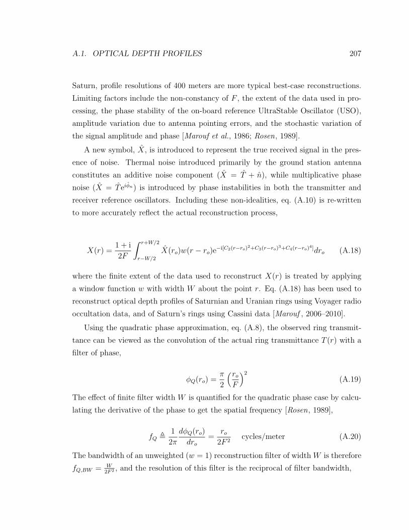
A.1. OPTICAL DEPTH PROFILES 207
Saturn, profile resolutions of 400 meters are more typical best-case reconstructions.
Limiting factors include the non-constancy of F , the extent of the data used in pro-
cessing, the phase stability of the on-board reference UltraStable Oscillator (USO),
amplitude variation due to antenna pointing errors, and the stochastic variation of
the signal amplitude and phase [Marouf et al., 1986; Rosen, 1989].
A new symbol, X, is introduced to represent the true received signal in the pres-
ence of noise. Thermal noise introduced primarily by the ground station antenna
constitutes an additive noise component (X = T + n), while multiplicative phase
noise (X = T eiφn) is introduced by phase instabilities in both the transmitter and
receiver reference oscillators. Including these non-idealities, eq. (A.10) is re-written
to more accurately reflect the actual reconstruction process,
X(r) =1 + i
2F
∫ r+W/2
r−W/2
X(ro)w(r − ro)e−i[C2(r−ro)2+C3(r−ro)3+C4(r−ro)4]dro (A.18)
where the finite extent of the data used to reconstruct X(r) is treated by applying
a window function w with width W about the point r. Eq. (A.18) has been used to
reconstruct optical depth profiles of Saturnian and Uranian rings using Voyager radio
occultation data, and of Saturn’s rings using Cassini data [Marouf , 2006–2010].
Using the quadratic phase approximation, eq. (A.8), the observed ring transmit-
tance can be viewed as the convolution of the actual ring transmittance T (r) with a
filter of phase,
φQ(ro) =π
2
(roF
)2(A.19)
The effect of finite filter width W is quantified for the quadratic phase case by calcu-
lating the derivative of the phase to get the spatial frequency [Rosen, 1989],
fQ 1
2π
dφQ(ro)
dro=
ro2F 2
cycles/meter (A.20)
The bandwidth of an unweighted (w = 1) reconstruction filter of width W is therefore
fQ,BW = W2F 2 , and the resolution of this filter is the reciprocal of filter bandwidth,

208 APPENDIX A. RADIO OCCULTATION OF PLANETARY RINGS
∆RW 1
fQ,BW
=2F 2
Wmeters (A.21)
Marouf et al. [1986] derive eq. (A.21) using a different approach.
The spatial sampling frequency is defined as the reciprocal of the radial sample
spacing, fs = ∆r−1o . In order to avoid aliasing in the reconstruction of the complex
transmittance, the filter bandwidth may not exceed the complex sampling frequency,
or fQ,BW ≤ fs. Thus a maximum is imposed upon the width of the reconstruction
filter,
Wmax =2F 2
∆ro(A.22)
When W = Wmax, the best possible resolution of ∆RWmin = ∆ro is achieved.
In practice, a window function other than w = 1 is applied to the filter in order to
reduce reconstruction artifacts induced by the effect of unwanted sidelobes, which
result from abrupt amplitude transitions at the edges of the window function. Strong
sidelobes in the filter function erode the dynamic range of the reconstruction process,
inhibiting the resolution of regions where transmittance changes abruptly, such as at
ring gap edges. Rosen studied the effect of windowing on profile reconstruction, and
discusses the associated issues in Rosen [1985] and Rosen [1989]. He determined that
the application of a Kaiser-Bessel window (with weighting parameter α = 2.5) offers a
reasonable tradeoff between resolution and sensitivity, improving the dynamic range
of the reconstruction process from 13dB to 57dB, while reducing the resolution to,
∆R ≈ 1.65∆RW (A.23)
Limitations on ∆R are also introduced by the variation and uncertainty of F
within the filter window W , and by the quadratic and quartic (4th-order polynomial)
phase approximations to ψ used in the reconstruction integrals of eq. (A.9) and eq.
(A.10), respectively. The interested reader is refered to Marouf et al. [1986] for a
detailed review of these effects.
Historically, eq. (A.18) with its quartic polynomial phase approximation was used

A.1. OPTICAL DEPTH PROFILES 209
to reconstruct ring transmittance profiles for Voyager 1’s observations of Saturn [Tyler
et al., 1983; Marouf et al., 1986; Rosen, 1989], and Voyager 2’s observations of Uranus
[Gresh et al., 1989; Gresh, 1990; Marouf , 2006–2010]. Theoretically, the polynomial
coefficients Cn are properly computed from derivatives of ψ during the Taylor series
analysis. In practice, this proved prohibitively difficult due to ψ’s functional depen-
dence on φs. Instead, the coefficients Cn in eq. (A.18) were determined using a fitting
algorithm, and the integral computed using numerical methods [Marouf et al., 1986].
The resolution of the reconstructed noisy profiles X(r) depend on the width W and
shape of the window. Longer window lengths W lead to higher resolution profiles, but
an accurate determination of φc is required over the full width of the window. Thus
the largest single limitation in the profile resolution is the accurate determination of
the phase φc over many seconds, thus enabling the use of a large data window W .
A.1.4 Profiling Ring Optical Depth
Since I/Io = |X|2, eq. (1.1) can be re-written as,
τq = − ln(X2
R +X2I
)(A.24)
where XR and XI are the real and imaginary components of the retrieved ring trans-
mittance in the presence of noise, respectively (X = XR + iXI). The phase shift
introduced in the coherent carrier wave is denoted φc,
φc = arctan
(XI
XR
)(A.25)
Uncertainty inherent in the noisy measurementX(r) of the true ring transmittance
T (r) sets limits on the confidence with which one can report the optical depth τ(r).
Marouf et al. [1986] defined confidence intervals for τ in terms of a threshold optical
depth τth,
τth = −µo ln (CPN/2) (A.26)
where PN is the post-reconstruction noise power, and C is a random variable that

210 APPENDIX A. RADIO OCCULTATION OF PLANETARY RINGS
has χ2 statistics and two degrees of freedom. For the Kaiser-Bessel window discussed
in Section A.1.3, the post-reconstruction noise power is given by,
PN = 0.32PNW
Wmax
= 0.32PN∆ro∆RW
(A.27)
which depends on the total noise power PN at a fixed sampling rate,
PN =1
SNRo
ro∆ro
(A.28)
SNRo is the free-space signal-to-noise ratio of the observation, integrated over a one-
second interval, and ro is the time rate-of-change of the ring plane intercept, also
known as the ring piercing point (RPP).
The confidence region is defined by Marouf et al. [1986] as a circle of radius√CPN/2 in the complex transmittance plane, centered on the true complex ring
transmittance T = TR + iTI ,
(XR − TR)2 + (XI − TI)
2 = CPN/2 (A.29)
The probability P (χ2 < C) that the noisy recovered complex ring transmittance X is
within the confidence region defines the confidence interval of τ , expressed in terms
of upper and lower bounding values. Marouf et al. [1986] report that for 50%, 70%,
and 90% confidence, C = 1.39, 2.41, and 4.61, respectively. In general, the confidence
interval of τ is given by [Marouf et al., 1986],
τL = τth − 2µo ln[e−(τ−τth)/(2µo) + 1
]0 ≤ τ ≤ ∞ (A.30)
τU =
⎧⎨⎩τth − 2µo ln[e−(τ−τth)/(2µo) − 1
]0 ≤ τ ≤ τth
∞ τ ≥ τth(A.31)
where τL and τU are the lower and upper confidence bounds on τ . Note that the
threshold optical depth τth discussed in this section and defined in eq. (A.26) is
different from the τth discussed in Section 6.4.2.

A.2. PARTICLE SIZE DISTRIBUTIONS 211
A.2 Particle Size Distributions
Radio occultation techniques provide estimates of the number density of ring parti-
cles of a given physical size contained in a ring system under study using two distinct
methods. First, large particles—particles ranging from a radius amin that is roughly
the size of the spacecraft antenna (Cassini’s high gain parabolic antenna has a diam-
eter of four meters), and up to radius amax that is limited by the spectral resolution
and corresponding SNR of the experiment—are sensed by analyzing the aggregate
forward scattering lobe of the received signal. Second, particles ranging in diameter
from decimeters down to the order of the shortest wavelength used in the experi-
ment are sensed by a comparison of the optical depth of the rings at two (or more)
frequencies [Marouf et al., 1982, 1983; Zebker et al., 1985].
Generally, the number density n(a) of particles in the rings are modeled as a
power-law distribution of the particle radius a,
n(a) =(aoa
)qn(ao) (A.32)
The parameter ao is chosen for convenience in fitting eq. (A.32) to the data, and
the power law index q controls the exponential rate at which the number density of
particles decreases as a function of their radius. The term n(a) is also referred to as
the particle size distribution. The general definition of n(a) is,
n(a) =dN(a)
daparticles/m2 per meter (A.33)
where N(a) is the cumulative distribution of all particles of radius ≤ a present in
a column of unit cross-sectional area perpendicular to the ring plane. The product
n(a)da is the number of particles of radii between a and a+ da existing in that same
column.
We now discuss both methods used to obtain particle size distributions: Analysis
of the near-forward scattered signal (suprameter-sized particles), and analysis of the
differential optical depth (submeter-sized particles).

212 APPENDIX A. RADIO OCCULTATION OF PLANETARY RINGS
A.2.1 Suprameter-Sized Particles
The incoherent component of the received radio occultation signal contains informa-
tion about the size of the particles that forward-scatter the transmitted signal to the
receiver. Following Marouf [1975], Marouf et al. [1982], and Marouf et al. [1983], the
power spectral density of the scattered signal of a given angular frequency ω, and at
a given time t, can be expressed as,
S(ω, t) =
∫spot
σd(β,r)G2(β, t)
|Rc − r|2 δ(ω − Ω(r)) dr (A.34)
where σd(β,r) is the differential scattering cross section of the rings per unit surface
area, β is the scattering angle relative to the Earth-spacecraft line of sight, G is the
spacecraft’s antenna gain pattern, and δ(ω − Ω(r)) is a delta function defining the
locus of points scattering at a particular frequency ω = Ω(r). Eq. (A.34) is formulated
for an uplink geometry, although the equation holds for a downlink configuration as
well due to reciprocity. The integration in eq. (A.34) is performed over the antenna
beam pattern, as it is projected on the rings.
If the contours of constant Doppler Ω are aligned with ringlet contours (be they
elliptical or circular), then the power scattered by a particular ringlet is given by,
Ps(t) ∫ ω2(t)
ω1(t)
S(ω, t) (A.35)
=
∫ringlet
σd(β)G2(β, t)
|Rc − r|2 δ(ω − Ω(r)) dr + ε (A.36)
where the error term ε is introduced primarily by misalignments between ringlet
features and the Doppler contours. The two frequencies ω1(t) and ω2(t) correspond
to the frequencies at the inner and outer edge of a ringlet feature. Eq. (A.36) can be
solved [Marouf et al., 1983; Zebker et al., 1983] to obtain the scattering cross section
σd(β), given the received signal time sequence and its corresponding geometry.
The shape of the scattering cross section σd(β) is a composite result of scattering
from the entire ensemble of particles that interact with the EM wave as it propagates
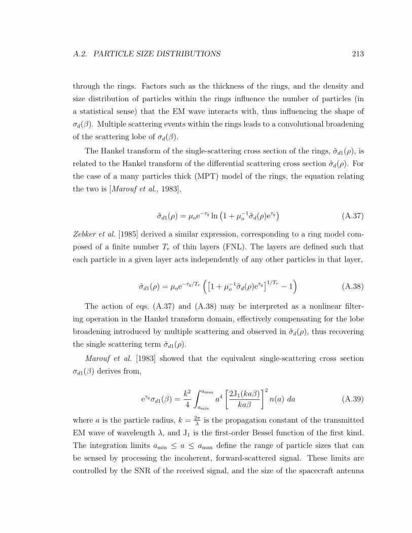
A.2. PARTICLE SIZE DISTRIBUTIONS 213
through the rings. Factors such as the thickness of the rings, and the density and
size distribution of particles within the rings influence the number of particles (in
a statistical sense) that the EM wave interacts with, thus influencing the shape of
σd(β). Multiple scattering events within the rings leads to a convolutional broadening
of the scattering lobe of σd(β).
The Hankel transform of the single-scattering cross section of the rings, σd1(ρ), is
related to the Hankel transform of the differential scattering cross section σd(ρ). For
the case of a many particles thick (MPT) model of the rings, the equation relating
the two is [Marouf et al., 1983],
σd1(ρ) = µoe−τq ln
(1 + µ−1
o σd(ρ)eτq)
(A.37)
Zebker et al. [1985] derived a similar expression, corresponding to a ring model com-
posed of a finite number Tr of thin layers (FNL). The layers are defined such that
each particle in a given layer acts independently of any other particles in that layer,
σd1(ρ) = µoe−τq/Tr
([1 + µ−1
o σd(ρ)eτq]1/Tr − 1
)(A.38)
The action of eqs. (A.37) and (A.38) may be interpreted as a nonlinear filter-
ing operation in the Hankel transform domain, effectively compensating for the lobe
broadening introduced by multiple scattering and observed in σd(ρ), thus recovering
the single scattering term σd1(ρ).
Marouf et al. [1983] showed that the equivalent single-scattering cross section
σd1(β) derives from,
eτqσd1(β) =k2
4
∫ amax
amin
a4[2J1(kaβ)
kaβ
]2n(a) da (A.39)
where a is the particle radius, k = 2πλ
is the propagation constant of the transmitted
EM wave of wavelength λ, and J1 is the first-order Bessel function of the first kind.
The integration limits amin ≤ a ≤ amax define the range of particle sizes that can
be sensed by processing the incoherent, forward-scattered signal. These limits are
controlled by the SNR of the received signal, and the size of the spacecraft antenna

214 APPENDIX A. RADIO OCCULTATION OF PLANETARY RINGS
constrains amin as discussed above. Marouf et al. [1983] also show that the product
eτq σd1(ρ) can be related directly to particle size distribution models of ring systems,
eτq σd1(ρ) = π
∫ amax
amin
a2C
(λρ
a
)n(a) da (A.40)
where the function C(z) = (2/π)[cos−1(z) − z(1 − z2)1/2] for 0 ≤ z ≤ 1; C(z) = 0
elsewhere, arises from taking the Hankel transform of eq. (A.39) since,
H[
2J1(kaβ)
kaβ
]2=
4π
(ka)2C
(λρ
a
)(A.41)
The script letter H denotes the Hankel transform operation. Combining eq. (A.40)
with eqs. (A.37) and (A.38) yields two equations, corresponding to the MPT model
of the rings,
µo ln(1 + µ−1
o σd(ρ)eτq)= π
∫ amax
amin
a2C
(λρ
a
)n(a) da (A.42)
and to the FNL model of the rings,
µoTre−τq/Tr
([1 + µ−1
o σd(ρ)eτq]1/Tr − 1
)= π
∫ amax
amin
a2C
(λρ
a
)n(a) da (A.43)
The left-hand side of eqs. (A.42) and (A.43) are completely determined from the
data and the choice of ring thickness model (MPT or FNL). The right-hand side of
eqs. (A.42) and (A.43) are essentially determined by the number density n(a), which
may be recovered by inverting the integral equations above numerically. Alternatively,
the parameters ao and q in the power-law model of n(a), eq.(A.32), are adjusted in
an iterative process until the left-hand side of eqs. (A.42) and/or (A.43) matches the
right-hand side, thus fitting a power-law model of the particle size distribution in the
rings to the measured data.

A.2. PARTICLE SIZE DISTRIBUTIONS 215
A.2.2 Submeter-Sized Particles
The optical depth of the rings, as measured at a given wavelength, is related to the
particle size distribution n(a) and the extinction efficiency Qext(a, λ) of the rings,
τ(λ) =
∫ ∞
0
πa2Qext(a, λ)n(a)da (A.44)
for the MPT ring model [Marouf et al., 1982, 1983], and,
τ(λ) = 2µoN
[∫ ∞
0
πa2
2µoNQext(a, λ)n(a)da− 1
](A.45)
for the FNL model of the rings [Zebker et al., 1985]. For the purpose of calculation, it
is common (e.g., Marouf et al. [1983]) to model the ring particles as dielectric spheres
with an index of refraction m = m′ − im′′, and to compute Qext using Mie theory (a
brief introduction to Mie theory is presented in Chapter 3). The extinction efficiency
varies with aλfrom Qext(
aλ 1) 1 to Qext(
aλ 1) ≈ 2 (the so-called extinction
paradox). For Voyager at Saturn, the parameter amin was assumed to fall well within
the Rayleigh range of the shortest radio wavelength.
If we have optical depth measurements at two or more frequencies, then we can
take advantage of the dependence ofQext onaλto obtain an estimate of the populations
of different particle sizes. Taking the difference,
∆τ12 = τ(λ1)− τ(λ2) (A.46)
For a measured ∆τ , an assumed amin well within the Rayleigh range, and given
values of amax and q, one may re-arrange eq. (A.46) to solve for n(ao). Furthermore,
computing ∆ττ(λ1)
from the measured data yields q for a given amax [Marouf et al., 1983].
In principle, the differential phase,
∆φ12 = φ(λ1)−(λ2
λ1
)φ(λ2) (A.47)
can be used as an additional means to estimate the number density. Generally, ∆φ is
positive for a λ; ∆φ → 0 for a λ; and ∆φ < 0 suggests the presence of charged

216 APPENDIX A. RADIO OCCULTATION OF PLANETARY RINGS
particles [Gresh et al., 1989; Gresh, 1990].
For an assumed power law distribution, differential measurements of optical depth
place a lower bound on q, an upper bound amin, and constraints on the relationship
between q and amin between these bounds. Measures of differential optical depth
produced from Cassini data at three frequencies (S-, X-, and Ka-bands) were used
to make the image shown in Figure 2.3, which is color-coded to show the range of
particle sizes populating the rings.
A.2.3 Surface Mass Density and Ring Thickness
The local surface mass density of the rings can be estimated by measuring the wave-
length λw of spiral bending waves and density waves present in the ring system.
Bending and density waves are introduced in Section 2.1.2.
In the asymptotic far-field of a bending wave—i.e., far enough from the resonance
location for the wavelength of the disturbance to be relatively constant—the inviscid
(undamped) linear theory gives the following [de Pater and Lissauer , 2001; Shu,
1984],
λw =4π2Gσρ
m2θ[ωf − n(r)]− µ2(r)
(A.48)
For density waves, we have a similar expression,
λw =4π2Gσρ
m2θ[ωf − n(r)]− κ2(r)
(A.49)
where G= 6.67428 × 10⁻¹¹ m3kg−1s−2 is the universal gravitational constant, σρ is
the surface mass density of the rings, ωf is the forcing frequency of the wave, mθ
is the azimuthal symmetry number, µ(r) is the natural vertical oscillation frequency
of a ring particle, κ(r) is the natural epicyclic (radial) oscillation frequency of a ring
particle, and n(r) is the orbital angular frequency of a local ring particle. The quantity
µ(r) (κ(r)) is the frequency at which the Saturnian moon responsible for the local
resonance is tugging ring particles in a direction perpendicular to (radially within) the
ring plane, to excite the bending (density) wave. In reality, these waves are damped,

A.3. SUMMARY 217
since collisions between particles remove energy from the wave. The damping rate
can be used to estimate the thickness of the rings [de Pater and Lissauer , 2001].
If we have measurements of λw and we know which moon is responsible for the
wave, then eqs. (A.48) and (A.49) can be rearranged and solved to yield estimates
of σρ (e.g., Gresh et al. [1986]; Rosen [1989]; Rosen et al. [1991a, b]). Surface mass
density estimates can also be obtained from the number density estimates described
in Section A.2, subject to estimates or assumptions of the bulk density of the ring
particles [Marouf et al., 1983; Zebker et al., 1985; Rosen, 1989].
A.3 Summary
Radio occultation can provide rich information about the structure and physical prop-
erties of planetary rings. The information includes:
1. Reconstructed ring optical depth profiles. Theoretically, the diffraction-corrected
profiles can approach resolutions of approximately a few hundred meters for
Saturn’s rings, and few tens of meters for Uranus’ rings.
2. Identification of bending and density waves in the rings, and of their associated
forcing resonances.
3. Characterization of time-evolution and azimuthal asymmetry effects by process-
ing data from multiple occultations.
4. Supra-meter particle size distribution estimates derived from processing the
scattered signal.
5. Sub-meter particle size distribution estimates derived from differential optical
depth measurements.
6. Surface mass densities estimated from waves, and from number density (particle
size distribution) estimates.
7. Statistical characterization of fine-scale (length scales of tens to hundreds of
meters) microstructure, such a gravitational wakes and periodic microstructure,
by analysis of diffracted signals.

218 APPENDIX A. RADIO OCCULTATION OF PLANETARY RINGS

Appendix B
Cassini 2005 Radio Occultation
Timelines
In this appendix we present the predicted timeline of the Cassini REV 7, 8, 10, and 12
experiments [Marouf , 2006–2010]. We also show plots of the local elevation angle of
Cassini at the Goldstone (G), Canberra (C), and Madrid (M) DSN complexes during
REVs 7, 8, 10, and 12. In the plots, the term BOT stands for beginning of track,
which is the time that a DSN complex begins to track Cassini. Similarly, EOT stands
for end of track. The radio occultation observation time is shown in light blue at the
top of the elevation angle plots, for reference.
219

220 APPENDIX B. 2005 OBSERVATIONS
Rev 7
Cassin
i Radio
Scie
nce O
cculta
tion: E
vent T
imes o
n D
OY 1
22/1
23
Essam
Maro
uf &
Ric
hard
Fre
nch 4
/28/0
5
SCET U
TC
ERT U
TC
Pacific
Tim
e
OW
LT =
G
MT-7
hrs
Com
ments
1:1
8:0
37:0
0:0
0
Sta
rt LM
B; E
nable
Monopuls
e1:1
5:0
02:3
3:0
319:3
3:0
3TW
NC O
FF (1
-Way) T
hro
ughout
Dis
able
Monopuls
e2:2
4:5
73:4
3:0
020:4
3:0
0Blin
d p
oin
ting is
initia
lized b
y M
onopuls
e
Sta
rt Baselin
e2:2
6:3
43:4
4:3
720:4
4:3
7Fre
e-s
pace: ~
51, 3
9, 4
1 d
B-H
z @
X, S
, and K
a
Rin
g F
2:5
5:2
54:1
3:2
821:1
3:2
8N
arro
w is
ola
ted rin
g; n
ot m
uch e
ffect e
xpecte
d
Rin
g A
in3:0
0:4
34:1
8:4
621:1
8:4
6Sudden d
rop in
sig
nal le
vel
Enke G
ap
3:0
5:1
24:2
3:1
521:2
3:1
5Brie
f recovery
of s
trong s
ignal le
vel
Rin
g A
out
3:2
1:0
34:3
9:0
621:3
9:0
6Stro
ng s
ignal e
xpecte
d in
the C
assin
i Div
Rin
g B
in3:2
7:0
94:4
5:1
221:4
5:1
2Sig
nal le
vel d
rops s
ubsta
ntia
lly
Rin
g B
out
4:0
0:3
85:1
8:4
122:1
8:4
1Sig
nal le
vel th
rougout R
ing B
is u
nknow
n!
Rin
g C
out
4:2
3:1
35:4
1:1
622:4
1:1
6H
igh s
ignal le
vel b
ut w
ith fa
st flu
ctu
atio
ns
Enable
Monopuls
e4:2
5:2
75:4
3:3
022:4
3:3
0M
onopuls
e o
ffset u
sed to
rein
tializ
e b
lind
Dis
able
Monopuls
e4:2
6:1
75:4
4:2
022:4
4:2
0 b
lind p
oin
ting
Ionoshere
in4:2
8:4
05:4
6:4
322:4
6:4
3M
ultip
ath
? (m
ore
than o
ne s
pectra
l line?)
Tro
posphere
in4:3
8:5
95:5
7:0
222:5
7:0
2Sig
nal le
vel d
rops s
yste
matic
ally
and fa
st
End o
f Ingre
ss
5:1
4:3
46:3
2:3
723:3
2:3
7Sig
nal a
bsorb
ed in
Satu
rn's
atm
osphere
Behin
d S
atu
rn
Sta
rt of E
gre
ss
6:3
3:3
47:5
1:3
70:5
1:3
7Sig
nal le
vel b
uild
s u
p s
yste
matic
ally
Tro
posphere
out
7:0
3:5
08:2
1:5
31:2
1:5
3Poin
ting e
rror m
ay a
ffect fre
e-s
pace s
ignal le
vel
Rin
g C
in7:1
5:2
38:3
3:2
61:3
3:2
6Stro
ng, d
ynam
ically
changin
g s
ignal le
vel
Ionosphere
out
7:1
6:1
88:3
4:2
11:3
4:2
1M
ultip
ath
? (m
ore
than o
ne s
pectra
l line?)
Enable
Monopuls
e7:1
6:2
78:3
4:3
01:3
4:3
0 M
onopuls
e o
ffset u
sed to
rein
tializ
e b
lind
Dis
able
Monopuls
e7:1
7:0
78:3
5:1
01:3
5:1
0 b
lind p
oin
ting
Rin
g B
in7:3
7:3
28:5
5:3
51:5
5:3
5Sig
nal le
vel d
rops s
ubsta
ntia
lly
Rin
g B
out
8:0
9:3
89:2
7:4
12:2
7:4
1Sig
nal le
vel u
nknow
n (s
mall) th
roughout R
ing B
Rin
g A
in8:1
5:2
29:3
3:2
62:3
3:2
6Sig
na le
vel c
om
es b
ack u
p in
the C
assin
i Div
isio
n
Enke G
ap
8:3
0:0
09:4
8:0
32:4
8:0
3Cle
ar d
ynam
ic s
ignal th
roughout m
ost o
f Rin
g A
Rin
g A
out
8:3
4:0
49:5
2:0
92:5
2:0
9Sudden tra
nsitio
n to
free-s
pace s
ignal le
vel
Rin
g F
8:3
8:5
29:5
6:5
52:5
6:5
5Rin
gs F
is o
nly
dete
cta
ble
in p
ostp
rocessin
g
End o
f Baselin
e9:0
9:3
410:2
7:3
73:2
7:3
7Poin
ting e
rror m
ay a
ffect fre
e-s
pace s
ignal le
vel
Enable
Monopuls
e9:1
1:0
010:2
9:0
33:2
9:0
3To a
ssess b
lind p
oin
ting e
rror d
urin
g rin
gs e
gre
ss
End L
MB
10:3
9:0
011:5
7:0
34:5
7:0
3End o
f the ra
dio
occulta
tion e
xperim
ent
Note
: Som
e R
ing E
dges a
re k
now
n to
be n
oncirc
ula
r, whic
h w
ill affe
ct e
vent tim
es a
bove
Figu
reB.1:
Pred
ictedCassin
iREV
7Rad
ioOccu
ltationEven
tsTim
eline.
Figu
recou
rtesyEssam
Marou
f(SJSU)
andAseel
Anab
tawi(JPL).

221
Rev 8
Cass
ini Radio
Sci
ence
Occ
ultation:
Event
Tim
es
on D
OY 2
005-1
41
Ess
am
Maro
uf
5/1
9/0
5D
RAFT
SCET U
TC
ERT U
TC
Paci
fic
Tim
eO
WLT
=
GM
T-7
hrs
Com
ments
1:2
0:1
67:0
0:0
0
Sta
rt L
MB
2:5
9:4
44:2
0:0
021:2
0:0
0Eart
h p
oin
ed,
but
no D
SN
sta
tions
are
tra
ckin
g
DSS-3
4:
Begin
-of-
Tra
ck5:3
4:4
46:5
5:0
0-0
:05:0
0N
o d
ow
nlin
k u
ntil 08:1
1:1
4D
SS-3
4:
Enable
Monopuls
e6:5
0:5
88:1
1:1
41:1
1:1
4Cass
ini H
GA is
Eart
h p
oin
ted a
t th
is t
ime
Sta
rt B
ase
line
6:5
0:5
88:1
1:1
41:1
1:1
4Fr
ee-s
pace
: ~
51,
39,
41 d
B-H
z @
X,
S,
and K
aRin
g F
7:2
0:1
98:4
0:3
51:4
0:3
5N
arr
ow
iso
late
d r
ing;
not
much
eff
ect
expect
ed
Rin
g A
in
7:2
5:4
18:4
5:5
71:4
5:5
7Sudden d
rop in s
ignal le
vel
Enke G
ap
7:3
0:1
18:5
0:2
71:5
0:2
7Brief
reco
very
of
stro
ng s
ignal le
vel
Rin
g A
out
7:4
6:0
79:0
6:2
32:0
6:2
3Str
ong s
ignal expect
ed in t
he C
ass
ini D
ivD
SS-3
4:
Dis
able
Monopuls
e7:5
2:0
09:1
2:1
62:1
2:1
6 M
onopuls
e o
ffse
t use
d t
o intializ
e b
lind p
oin
ting
Rin
g B
in
7:5
2:1
59:1
2:3
12:1
2:3
1Sig
nal le
vel dro
ps
subst
antially
DSS-5
5:
Begin
-of-
Tra
ck7:5
4:4
49:1
5:0
02:1
5:0
0In
Rin
g B
; on b
lind p
oin
ting t
ill e
xit f
rom
Rin
g B
Rin
g B
out
8:2
5:4
99:4
6:0
52:4
6:0
5Sig
nal le
vel in
Rin
g B
is
sm
all
DSS-3
4:
Enable
Monopuls
e8:2
6:0
09:4
6:1
62:4
6:1
6M
onopuls
e e
nable
d ~
10 s
ec
aft
ere
xit f
rom
Rin
g B
DSS-5
5:
Enable
Monopuls
e8:2
6:0
09:4
6:1
62:4
6:1
6M
onopuls
e e
nable
d ~
10 s
ec
aft
ere
xit f
rom
Rin
g B
Rin
g C
out
8:4
8:2
210:0
8:3
83:0
8:3
8H
igh s
ignal le
vel but
with f
ast
flu
ctuations
DSS-3
4:
End-o
f-Tra
ck8:4
9:4
410:1
0:0
03:1
0:0
0Canberr
a s
ets
during t
he o
ccultation p
eriod
DSS-5
5:
Dis
able
Monopuls
e8:5
2:3
010:1
2:4
63:1
2:4
6 M
onopuls
e o
ffse
t use
d t
o intializ
e b
lind p
oin
ting
Ionosh
ere
in
8:5
4:3
010:1
4:4
63:1
4:4
6Str
ong s
ignal le
vel
Tro
posp
here
in
9:0
6:0
010:2
6:1
63:2
6:1
6Sig
nal le
vel dro
ps
syst
em
atica
lly a
nd f
ast
End o
f In
gre
ss9:3
2:5
810:5
3:1
43:5
3:1
4Sig
nal abso
rbed in S
atu
rn's
atm
osp
here
Behin
d S
atu
rnSta
rt o
f Egre
ss11:0
0:5
812:2
1:1
45:2
1:1
4Sig
nal le
vel build
s up s
yst
em
atica
llyTro
posp
here
out
11:3
3:0
012:5
3:1
65:5
3:1
6Poin
ting e
rror
may a
ffect
fre
e-s
pace
sig
nal le
vel
Ionosp
here
out
11:4
4:4
913:0
5:0
56:0
5:0
5Str
ong s
ignal le
vel
DSS-5
5:
Enable
Monopuls
e11:4
3:3
013:0
3:4
66:0
3:4
6M
onopuls
e e
nable
d ~
1 m
befo
re R
ing C
Rin
g C
in
11:4
4:3
213:0
4:4
86:0
4:4
8Str
ong,
dynam
ically
changin
g s
ignal le
vel
DSS-5
5:
Dis
able
Monopuls
e12:0
6:2
913:2
6:4
56:2
6:4
5 M
onopuls
e o
ffse
t use
d t
o intializ
e b
lind p
oin
ting
Rin
g B
in
12:0
6:3
913:2
6:5
56:2
6:5
5Sig
nal le
vel dro
ps
subst
antially
Rin
g B
out
12:3
8:5
013:5
9:0
66:5
9:0
6Sig
nal le
vel is
sm
all
in R
ing B
DSS-5
5:
Enable
Monopuls
e12:3
9:0
013:5
9:1
66:5
9:1
6M
onopuls
e e
nable
d ~
10 s
ec
aft
ere
xit f
rom
Rin
g B
Rin
g A
in
12:4
5:3
514:0
5:5
17:0
5:5
1Sig
na level co
mes
back
up in t
he C
ass
ini D
ivis
ion
Enke G
ap
12:5
9:1
714:1
9:3
37:1
9:3
3Cle
ar
dynam
ic s
ignal th
roughout
most
of
Rin
g A
Rin
g A
out
13:0
3:2
214:2
3:3
87:2
3:3
8Sudden t
ransi
tion t
o f
ree-s
pace
sig
nal le
vel
Rin
g F
13:0
8:1
214:2
8:2
87:2
8:2
8Rin
gs
F is
only
dete
ctable
in p
ost
pro
cess
ing
End o
f Base
line
13:3
8:5
814:5
9:1
47:5
9:1
4Str
ong s
ignal le
vel
End L
MB
14:4
7:4
416:0
8:0
09:0
8:0
0End o
f th
e r
ev 8
radio
occ
ultation e
xperim
ent
Note
: Som
e R
ing E
dges
are
know
n t
o b
e n
onci
rcula
r, w
hic
h w
ill a
ffect
event
tim
es
above
Figure
B.2:PredictedCassiniREV
8Rad
ioOccultationEvents
Tim
eline.
Figure
courtesyEssam
Marou
f(SJSU)
andAseel
Anab
tawi(JPL).

222 APPENDIX B. 2005 OBSERVATIONS
Rev 1
0 C
assini R
adio
Scien
ce Occu
ltation: E
vent T
imes o
n D
OY 1
77-1
78, 2
005
Essam
Maro
uf 5
/23/0
5
SCET U
TC
ERT U
TC
Pacific T
ime
OW
LT =
G
MT-7
hrs
Com
men
ts1:2
3:1
77:0
0:0
0
DSS-2
6: B
egin
-of-T
rack15:5
6:4
317:2
0:0
010:2
0:0
0Cassin
i HG
A is n
ot E
arth p
oin
edD
SS-2
5: B
egin
-of-T
rack16:1
1:4
317:3
5:0
010:3
5:0
0Cassin
i HG
A is n
ot E
arth p
oin
edStart LM
B16:2
9:0
017:5
2:1
710:5
2:1
7Cassin
i HG
A E
arth p
oin
ing starts
DSS-2
5: E
nab
le Monopulse?
16:2
9:4
317:5
3:0
010:5
3:0
0Enab
le monopulse A
SAP after B
OT
DSS-2
6: E
nab
le Monopulse
16:2
9:4
317:5
3:0
010:5
3:0
0Enab
le monopulse A
SAP after B
OT
Start B
aseline
16:5
2:3
018:1
5:4
711:1
5:4
7Start o
f the R
SS o
ccultatio
n exp
erimen
tRin
g F
17:1
9:5
818:4
3:1
511:4
3:1
5Rin
gs F is o
nly d
etectable in
postp
rocessin
gRin
g A
in17:2
5:2
418:4
8:4
111:4
8:4
1Sudden
dro
p in
signal level
Enke G
ap17:2
9:5
818:5
3:1
511:5
3:1
5Brief reco
very of stro
ng sig
nal level
Rin
g A
out
17:4
6:0
719:0
9:2
412:0
9:2
4Stro
ng sig
nal exp
ected in
the C
assini D
ivD
SS-2
5: D
isable M
onopulse?
17:5
1:5
019:1
5:0
712:1
5:0
7 M
onopulse o
ffset used
to rein
tialize blin
d p
ntn
gD
SS-2
6: D
isable M
onopulse
17:5
1:5
019:1
5:0
712:1
5:0
7 M
onopulse o
ffset used
to rein
tialize blin
d p
ntn
gRin
g B
in17:5
2:2
019:1
5:3
712:1
5:3
7Sig
nal level d
rops su
bstan
tiallyRin
g B
out
18:2
6:1
719:4
9:3
412:4
9:3
4Sig
nal level th
roughout R
ing B
is small
DSS-2
5: E
nab
le Monopulse?
18:2
6:4
719:5
0:0
412:5
0:0
4M
onopulse en
abled
~30 s after exit fro
m R
ing B
DSS-2
6: E
nab
le Monopulse
18:2
6:4
719:5
0:0
412:5
0:0
4M
onopulse en
abled
~30 s after exit fro
m R
ing B
Rin
g C
out
18:4
9:0
020:1
2:1
713:1
2:1
7H
igh sig
nal level b
ut w
ith fast flu
ctuatio
ns
DSS-2
5: D
isable M
onopulse?
18:5
6:0
020:1
9:1
713:1
9:1
7 M
onopulse o
ffset used
to rein
tialize blin
d p
ntn
g
DSS-2
6: D
isable M
onopulse
18:5
6:0
020:1
9:1
713:1
9:1
7 M
onopulse o
ffset used
to rein
tialize blin
d p
ntn
gIo
nosh
ere in18:5
7:5
820:2
1:1
513:2
1:1
5Stro
ng sig
nal level
Tro
posp
here in
19:0
7:2
820:3
0:4
513:3
0:4
5Sig
nal level d
rops system
aticallyKa-B
and sig
nal lo
ss19:1
3:2
820:3
6:4
513:3
6:4
5Likely d
isappearan
ce of th
e Ka-b
and sig
nal
X-b
and sig
nal lo
ss19:1
4:5
820:3
8:1
513:3
8:1
5Likely d
isappearan
ce of th
e X-b
and sig
nal
S-b
and sig
nal lo
ss19:1
6:0
820:3
9:2
513:3
9:2
5Likely d
isappearan
ce of th
e S-b
and sig
nal
End o
f Ingress
19:3
7:3
021:0
0:4
714:0
0:4
7End o
f Satu
rn in
gress o
ccultatio
nBeh
ind S
aturn
Figu
reB.3:
Pred
ictedCassin
iREV
10Ingress
Rad
ioOccu
ltationEven
tsTim
eline.
Figu
recou
rtesyEssam
Marou
f(SJSU)an
dAseel
Anab
tawi(JPL).

223
Behin
d S
atu
rnSta
rt o
f Egre
ss21:0
9:3
022:3
2:4
715:3
2:4
7Sta
rt o
f Satu
rn e
gre
ss o
ccultation
Expect
ed w
eak S
-Band s
igna
21:3
1:5
022:5
5:0
715:5
5:0
7S-B
and s
tart
s to
build
up s
yst
em
atica
llyExpect
ed w
eak X
-band s
igna
21:3
3:0
022:5
6:1
715:5
6:1
7X-B
and level st
art
s to
build
up s
yst
em
atica
llyExpect
ed w
eak K
a-b
and s
ig21:3
4:2
922:5
7:4
615:5
7:4
6Ka-B
and level st
art
s to
build
up s
yst
em
atica
llyTro
posp
here
out
21:4
0:2
923:0
3:4
616:0
3:4
6Blin
d p
oin
ting e
rror
may a
ffect
sig
nal le
vel
Ionosp
here
out
21:4
9:4
923:1
3:0
616:1
3:0
6Str
ong s
ignal le
vel
DSS-2
5:
Enable
Monopuls
e?
21:5
1:0
023:1
4:1
716:1
4:1
7M
onopuls
e e
nable
d ~
3 m
befo
re R
ing C
DSS-2
6:
Enable
Monopuls
e21:5
1:0
023:1
4:1
716:1
4:1
7M
onopuls
e e
nable
d ~
3 m
befo
re R
ing C
Rin
g C
in
21:5
3:4
323:1
7:0
016:1
7:0
0Str
ong d
ynam
ically
changin
g s
ignal le
vel
DSS-2
5:
Dis
able
Monopuls
e?
22:1
5:2
923:3
8:4
616:3
8:4
6 M
onopuls
e o
ffse
t use
d t
o r
ein
tializ
e b
lind
DSS-2
6:
Dis
able
Monopuls
e22:1
5:2
923:3
8:4
616:3
8:4
6 M
onopuls
e o
ffse
t use
d t
o r
ein
tializ
e b
lind
Rin
g B
in
22:1
5:5
923:3
9:1
616:3
9:1
6Sig
nal le
vel dro
ps
subst
antially
Rin
g B
out
22:4
8:3
40:1
1:5
117:1
1:5
1Sig
nal le
vel is
sm
all
in R
ing B
DSS-2
5:
Enable
Monopuls
e?
22:4
9:0
40:1
2:2
117:1
2:2
1M
onopuls
e e
nable
d ~
30 s
aft
er
exit f
rom
Rin
g B
DSS-2
6:
Enable
Monopuls
e22:4
9:0
40:1
2:2
117:1
2:2
1M
onopuls
e e
nable
d ~
30 s
aft
er
exit f
rom
Rin
g B
Rin
g A
in
22:5
4:2
40:1
7:4
117:1
7:4
1Sig
nal le
vel co
mes
back
up in t
he C
ass
ini D
ivis
ion
Enke G
ap
23:0
9:2
00:3
2:3
717:3
2:3
7Cle
ar
dynam
ic s
ignal th
roughout
most
of
Rin
g A
Rin
g A
out
23:1
3:2
90:3
6:4
617:3
6:4
6Sudden t
ransi
tion t
o f
ree-s
pace
sig
nal le
vel
Rin
g F
23:1
8:2
30:4
1:4
017:4
1:4
0Rin
gs
F is
only
dete
ctable
in p
ost
pro
cess
ing
End o
f Base
line
23:5
1:0
01:1
4:1
718:1
4:1
7End o
f th
e r
ev 1
0 r
adio
occ
ultation e
xperim
ent
End L
MB
0:2
0:0
61:4
3:2
318:4
3:2
3End o
f Eart
h p
oin
ting p
eriod
DSS-2
5:
End-o
f-Tra
ck0:3
1:4
31:5
5:0
018:5
5:0
0D
SS-2
6:
End-o
f-Tra
ck0:4
6:4
32:1
0:0
019:1
0:0
0N
ote
: Som
e R
ing E
dges
are
know
n t
o b
e n
onci
rcula
r, w
hic
h w
ill a
ffect
event
tim
es
above
Figure
B.4:PredictedCassiniREV
10EgressRad
ioOccultationEvents
Tim
eline.
Figure
courtesyEssam
Marou
f(SJSU)an
dAseel
Anab
tawi(JPL).

224 APPENDIX B. 2005 OBSERVATIONS
Rev 1
2 C
assin
i Radio
Scie
nce O
cculta
tion: E
vent T
imes o
n D
OY 2
14, 2
005
Essam
Maro
uf 7
/29/0
5
SCET U
TC
ERT U
TC
Pacific
Tim
e
OW
LT =
G
MT-7
hrs
Com
ments
1:2
3:5
57:0
0:0
0
DSS-5
5: B
egin
-of-T
rack
6:3
6:0
58:0
0:0
01:0
0:0
0Cassin
i HG
A is
not E
arth
poin
ed
Sta
rt LM
B6:5
7:0
08:2
0:5
51:2
0:5
5Cassin
i HG
A E
arth
poin
ing s
tarts
DSS-5
5: E
nable
Monopuls
e6:5
7:0
08:2
0:5
51:2
0:5
5Enable
monopuls
e A
SAP a
fter B
OT
Sta
rt Baselin
e7:3
1:1
68:5
5:1
11:5
5:1
1Sta
rt of th
e R
SS o
cculta
tion e
xperim
ent
Rin
g F
7:5
3:4
09:1
7:3
52:1
7:3
5Rin
g F
is o
nly
dete
cta
ble
in p
ostp
rocessin
g
Rin
g A
in7:5
9:1
29:2
3:0
72:2
3:0
7Sudden d
rop in
sig
nal le
vel
Enke G
ap
8:0
3:5
19:2
7:4
62:2
7:4
6Brie
f recovery
of s
trong s
ignal le
vel
Rin
g A
out
8:2
0:1
99:4
4:1
42:4
4:1
4Stro
ng s
ignal e
xpecte
d in
the C
assin
i Div
DSS-5
5: D
isable
Monopuls
e8:2
6:0
99:5
0:0
42:5
0:0
4 M
onopuls
e o
ffset u
sed to
rein
tializ
e b
lind p
ntn
g
Rin
g B
in8:2
6:3
99:5
0:3
42:5
0:3
4Sig
nal le
vel d
rops s
ubsta
ntia
lly
Rin
g B
out
9:0
1:2
410:2
5:1
93:2
5:1
9Sig
nal le
vel th
roughout R
ing B
is s
mall
DSS-5
5: E
nable
Monopuls
e9:0
1:5
410:2
5:4
93:4
8:3
6M
onopuls
e e
nable
d ~
30 s
afte
r exit fro
m R
ing B
Rin
g C
out
9:2
4:4
110:4
8:3
63:4
8:3
6H
igh s
ignal le
vel b
ut w
ith fa
st flu
ctu
atio
ns
DSS-5
5: D
isable
Monopuls
e9:2
7:0
510:5
1:0
03:5
1:0
0 M
onopuls
e o
ffset u
sed to
rein
tializ
e b
lind p
ntn
g
Ionoshere
in9:2
7:3
010:5
1:2
53:5
1:2
5im
apcat p
ara
mete
r ~68,0
00 k
m
Tro
posphere
in9:3
7:5
811:0
1:5
34:0
1:5
3Sig
nal le
vel d
rops s
yste
matic
ally
loss o
f Ka-B
and s
ignal
9:4
3:4
611:0
7:4
14:0
7:4
1Lik
ely
dis
appeara
nce o
f the K
a-b
and s
ignal
loss o
f X-b
and s
ignal
9:4
4:4
611:0
8:4
14:0
8:4
1Lik
ely
dis
appeara
nce o
f the X
-band s
ignal
loss o
f S-b
and s
ignal
9:4
5:5
611:0
9:5
14:0
9:5
1Lik
ely
dis
appeara
nce o
f the S
-band s
ignal
End o
f Ingre
ss
10:0
8:1
611:3
2:1
14:3
2:1
1End o
f Satu
rn in
gre
ss o
cculta
tion
Behin
d S
atu
rn
Figu
reB.5:
Pred
ictedCassin
iREV
12Ingress
Rad
ioOccu
ltationEven
tsTim
eline.
Figu
recou
rtesyEssam
Marou
f(SJSU)an
dAseel
Anab
tawi(JPL).

225
Behin
d S
atu
rn
Sta
rt o
f Egre
ss
11:3
8:1
613:0
2:1
16:0
2:1
1Sta
rt o
f Satu
rn e
gre
ss o
ccultation
weak S
-Band s
ignal
12:0
7:1
013:3
1:0
56:3
1:0
5S-B
and s
tart
s t
o b
uild u
p s
yste
matically
weak X
-band s
ignal
12:0
8:1
013:3
2:0
56:3
2:0
5X-B
and level sta
rts t
o b
uild u
p s
yste
matically
weak K
a-b
and s
ignal
12:0
9:4
413:3
3:3
96:3
3:3
9Ka-B
and level sta
rts t
o b
uild u
p s
yste
matically
Tro
posphere
out
12:1
6:2
913:4
0:2
46:4
0:2
4Blind p
oin
ting e
rror
may a
ffect
sig
nal le
vel
Ionosphere
out
12:2
6:4
113:5
0:3
66:5
0:3
6Str
ong s
ignal le
vel
DSS-5
5:
Enable
Monopuls
e12:3
4:1
213:5
1:0
06:5
1:0
0im
pact
para
mete
r >
68,0
00 k
m
Rin
g C
in
12:3
4:1
213:5
8:0
76:5
8:0
7Str
ong d
ynam
ically c
hangin
g s
ignal le
vel
DSS-5
5:
Dis
able
Monopuls
e12:5
6:3
414:2
0:2
97:2
0:2
9 M
onopuls
e o
ffset
used t
o r
ein
tialize b
lind
Rin
g B
in
12:5
7:0
414:2
0:5
97:2
0:5
9Sig
nal le
vel dro
ps s
ubsta
ntially
Rin
g B
out
13:3
0:3
014:5
4:2
57:5
4:2
5Sig
nal le
vel is
sm
all in R
ing B
DSS-5
5:
Enable
Monopuls
e13:3
1:0
014:5
4:5
57:5
4:5
5M
onopuls
e e
nable
d ~
30 s
aft
er
exit f
rom
Rin
g B
Rin
g A
in
13:3
6:2
815:0
0:2
38:0
0:2
3Sig
nal le
vel com
es b
ack u
p in t
he C
assin
i D
ivis
ion
Enke G
ap
13:5
1:4
615:1
5:4
18:1
5:4
1Cle
ar
dynam
ic s
ignal th
roughout
most
of
Rin
g A
Rin
g A
out
13:5
6:0
115:1
9:5
68:1
9:5
6Sudden t
ransitio
n t
o f
ree-s
pace s
ignal le
vel
Rin
g F
14:0
1:0
215:2
4:5
78:2
4:5
7Rin
gs F
is o
nly
dete
cta
ble
in p
ostp
rocessin
g
End o
f Baseline
14:2
9:1
615:5
3:1
18:5
3:1
1End o
f th
e r
ev 1
0 r
adio
occultation e
xperim
ent
End L
MB
15:0
7:0
416:3
0:5
99:3
0:5
9H
GA C
ontinues t
o b
e E
art
h p
oin
ted
DSS-5
5:
End-o
f-Tra
ck
15:2
6:0
516:5
0:0
09:5
0:0
0G
ravity E
nhancem
ent
Observ
ation d
uring D
L
Note
: Som
e R
ing E
dges a
re k
now
n t
o b
e n
oncircula
r, w
hic
h w
ill aff
ect
event
tim
es a
bove
Enable
/Dis
able
monopuls
e s
trate
gy is t
enta
tive a
t th
is t
ime;
may b
e c
hanged in r
eal-
tim
e
Figure
B.6:PredictedCassiniREV
12EgressRad
ioOccultationEvents
Tim
eline.
Figure
courtesyEssam
Marou
f(SJSU)an
dAseel
Anab
tawi(JPL).

226 APPENDIX B. 2005 OBSERVATIONS
0 10 20 30 40 50 60 70 80 901:002:00
3:004:00
5:006:00
7:008:00
9:0010:00
11:0012:00
Time (ER
T-UTC
)
Elevation Angle (Degrees)
S10 Rev 7 R
ing-Saturn (I & E) O
ccultation2005-123 / M
ay 03, 2005
G
C
M
EO
TB
OT
EO
T
BO
Tobservatio
Figu
reB.7:
Cassin
iREV
7Local
Elevation
Angle
atDSN
Receiv
ingStation
s.Figu
recou
rtesyAseel
Anab
tawi
(JPL).

227
0102030405060708090
5:00
6:00
7:00
8:00
9:00
10:0
011
:00
12:0
013
:00
14:0
015
:00
16:0
0Ti
me
(ER
T-U
TC)
Elevation Angle (Degrees)
S11
Rev
8 R
ing-
Satu
rn (I
& E
) Occ
ulta
tion
2005
-141
/ M
ay 2
1, 2
005
obse
rvat
ion
C
M
BO
EO
T
BO
TE
OT
Figure
B.8:CassiniREV
8LocalElevation
Angleat
DSN
ReceivingStation
s.Figure
courtesyAseel
Anab
tawi
(JPL).

228 APPENDIX B. 2005 OBSERVATIONS
0 10 20 30 40 50 60 70 80 9015:0016:00
17:0018:00
19:0020:00
21:0022:00
23:000:00
1:002:00
3:00Tim
e (ERT-U
TC)
Elevation Angle (Degrees)
G
S12 Rev 10 R
ing-Saturn (I & E) O
ccultation2005-177 / June 26, 2005
observation
BO
TE
OT
M
C
Figu
reB.9:
Cassin
iREV
10Local
Elevation
Angle
atDSN
Receiv
ingStation
s.Figu
recou
rtesyAseel
Anab
tawi
(JPL).

229
0102030405060708090
6:00
7:00
8:00
9:00
10:00
11:00
12:00
13:00
14:00
15:00
16:00
17:00
18:00
Tim
e (E
RT-
UTC
)
Elevation Angle (Degrees)
G
S13
Rev
12
Rin
g-Sa
turn
(I &
E) O
ccul
tatio
n20
05-2
14 /
Aug
ust 2
, 200
5observation
M
BOT
EOT
BOT
GravityEnhancement
Figure
B.10:
CassiniREV
12LocalElevation
Angleat
DSN
ReceivingStation
s.Figure
courtesyAseel
Anab
tawi
(JPL).

230 APPENDIX B. 2005 OBSERVATIONS

Appendix C
Historically Important Articles on
Saturn’s Rings
The translated text contained in this appendix is courtesy of Dr. John O’Connor,
Mathematical Institute, University of St. Andrews (Scotland). I am very grateful to
him for making this material available to me.
C.1 Christiaan Huygens’ article on Saturn’s Ring
In 1659, Christiaan Huygens published an article on Saturn’s Ring in Systema Sat-
urnium. The text below is based on a translation from the original latin, completed
by J. H. Walden in 1928.
Excerpt from Systema Saturnium
When Galileo made use of the telescope, noblest invention of nation of Belgium, for
observation of the heavenly bodies, and, before all other men, disclosed to mortals
those very celebrated phenomena of the planets, the most wonderful of his discoveries,
it would seem, were those relating to the star of Saturn. For all the other phenomena,
though justly calling for our wonder and admiration, were still not of a kind to
make it necessary to question strongly the causes of their existence. But Saturn’s
231
232 APPENDIX C. HISTORICAL ARTICLES
changing forms showed a new and strange device of nature, the principle of which
neither Galileo himself nor, in all the time since, any of the astronomers (with their
permission be it said) has succeeded in divining. Galileo had first seen this star
shining, not as a single disk, but in what seemed to be a triple form, as two smaller
stars in close proximity to, and on opposite sides of, a larger star, in line with its
centre. And seeing this form continue for nearly three years with no change, he had
become firmly convinced that, just as Jupiter was provided with four satellites, so
Saturn was provided with two, which, however, had no motion, and so would always
cling to the sides of Saturn in the same position. But when Saturn came forth alone,
quite destitute of his former retinue of satellites, Galileo was obliged to change his
opinion. Astonished by what he saw, he tried to reach by conjecture the cause of the
appearance, and made a few predictions as to the time when the former phase was
due to recur. But, it was shown by the event, these predictions were not then fulfilled
according to his expectation, nor, it appeared, was Saturn satisfied with having only
two aspects. For a succession of other strange and marvellous forms was revealed,
which I find first described by Josephus Blancanus and Franciscus Fontana - forms
of such unusual appearance that they were considered by many as a mockery of the
eyes, shapes adhering to the lenses rather than existing in the heavens; but after the
same forms had been seen by more, it became clear that it was no false evidence that
revealed them.
And so I was also drawn by an urgent longing to behold these wonders of the
heaven. But I had only the ordinary form of telescope, which measured five or six
feet in length. I, therefore, set myself to work with all the earnestness and seriousness
I could command to learn the art by which glasses are fashioned for these uses,
and I did not regret having put my own hand to the task. After overcoming great
difficulties (for this art has in reserve more difficulties than it seems to bear on its
face), I at last succeeded in making the lenses which have provided me with the
material for writing this account. For upon immediately directing my telescope at
Saturn, I found that things there had quite a different appearance from that which
they had previously been thought by most men to have. For it appeared that the two
neighbouring appendages clinging to Saturn were by no means two planets, but rather

C.1. CHRISTIAAN HUYGENS’ ARTICLE ON SATURN’S RING 233
something different, while, distinct from these, there was a single planet, at a greater
distance from Saturn and revolving around him in sixteen days; and the existence of
this planet had been unknown through all the centuries up to that time. Following
the wise advice of a distinguished man, one equally conspicuous for his ability and
his character, Johannes Capellanus, I three years ago informed astronomers of my
new observation. For while I was sojourning at Paris, I told Capellanus, as well as
Gassendi and others, of the satellite of Saturn which I had seen, and Capellanus gave
me many reasons for believing that I ought not to withhold an announcement that
would be so pleasing to all men until I should finish the work on the complete System
of Saturn, which I was then engaged upon. And so, on the 5th day of March [later in
the article Huygens says it was the twenty-fifth of March, so one of these is a misprint],
I in the year 1656, I put forth the result of my observation on the Moon of Saturn (for
so I have quite properly named the, new star), and, together with it, an hypothesis
containing an explanation of the other phenomena of Saturn; in the case of the latter,
however, I confused the order of the letters in which it was written, that it might
witness to the fact simply that I was not unacquainted with it at that time, and also
that others might be induced in this way to publish the results of their speculations
and might not complain that the glory of the discovery had been snatched from them.
Afterwards, however, in response to the request of the same distinguished man, I also
solved this literary riddle, and set before him in outline the entire hypothesis; whence
perhaps my theory about the phases of Saturn has already found its way to the ears
of others. But, in any case, the wonderful and unusual creation of nature shown in
connection with this planet demands a fuller treatment, and I ought not to expect
that either my account of the phenomena or the assumptions I make for explaining
them will gain general support unless it is seen that the latter, rest on the principles of
reasoning, and the former is backed by the evidence of observation. Therefore, I now
propose to fulfil both of these requirements. And, in the first place, I will determine
as accurately as possible from my observations the facts which have to do with the
motion and the period of revolution of the planet’s satellite, and I will construct
tables of its motion. Then I will assign the various phases of Saturn himself to their
separate causes, that thus we may have a ready means of determining beforehand
234 APPENDIX C. HISTORICAL ARTICLES
what the future phases will be ...
That neither you [Hodierna] nor those distinguished men whose opinions I have
previously reviewed have reached the truth of the matter, is not at all to be wondered
at or to be imputed to you as a fault, since for the most part false phenomena were
reported to you as true, and other phenomena which were observed in connection
with Saturn, free from the deception of sight, did not come to your notice at all. If
you had been so fortunate as to observe these phenomena with me, it is reasonable to
suppose that you would have drawn from them the same conclusions with regard to
the real form of the planet that I have. Now I was greatly helped in this matter not
only by those more genuine phases, but also by the motion of Saturn’s Moon, which
I observed from the beginning; indeed it was the revolution of this Moon around
Saturn that first caused to dawn upon me the hope of constructing the hypothesis.
The nature of this hypothesis I will proceed to explain in what follows.
When, then, I had discovered that the new planet revolved around Saturn in a
period of sixteen days, I thought that without any doubt Saturn rotated on his own
axis in even less time. For even before this I had always believed that the other
primary planets were like our Earth in this respect that each rotated on its own axis,
and so the entire surface rejoiced in the light of the Sun, a part at a time; and,
more than this, I believe that in general the arrangement with the large bodies of the
world was such that those around which smaller bodies revolved, having themselves
a central position, had also a shorter period of rotation. Thus the Sun, its spots
declare, rotates on its own axis in about twenty-six days; but around the Sun the
various planets, among which the Earth is also to be reckoned, complete their courses
in times varying as their distances. Again, this Earth rotates in daily course, and
around the Earth the Moon circles with monthly motion. Around the planet Jupiter
four smaller planets, that is to say Moons, revolve, subject to this same law, under
which the velocities increase as the distances diminish. Whence, indeed, we must
conclude perhaps that Jupiter rotates in a shorter time than 24 hours, since his
nearest Moon requires less than two days. Now having long since learned all these
facts, I concluded even then that Saturn must have a similar motion. But it was my
observation in regard to his satellite that gave me the information about the velocity
C.1. CHRISTIAAN HUYGENS’ ARTICLE ON SATURN’S RING 235
of his motion of rotation. The fact that the satellite completes its orbit in sixteen
days leads to the conclusion that Saturn, being in the centre of the satellite’s orbit,
rotates in much less time. Furthermore, the following conclusion seemed reasonable:
that all the celestial matter that lies between Saturn and his satellite is subject to
the same motion, in this way that the nearer it is to Saturn, the nearer it approaches
Saturn’s velocity. Whence, finally, the following resulted: the appendages also, or
arms, of Saturn are either joined and attached to the globular body at its middle and
go around with it, or, if they are separated by a certain distance, still revolve at a
rate not much inferior to that of Saturn.
Furthermore, while I was considering these facts in connection with the motion of
the arms, these arms appeared under the aspect which was exhibited at the time of
my previous observations of the year 1655. The body of Saturn at its middle was quite
round, while the arms extended on either side along the same straight line, as though
the planet were pierced through the middle by a kind of axis; although, as indicated
in the first figure of all, these arms, as seen through the twelve-foot telescope that
I was then using, appeared a little thicker and brighter toward the ends on either
side of the planet than they did where they joined the middle of the sphere. When,
therefore, the planet continued day after day to present this same aspect, I came to
understand that, inasmuch as the circuit of Saturn and the adhering bodies was so
short, this could happen under no other condition than that the globe of Saturn were
assumed to be surrounded equally on all sides by another body, and that thus a kind
of ring encircled it about the middle; for so, with whatever velocity it revolved, it
would always present the same aspect to us, if, of course, its axis were perpendicular
to the plane of the ring.
And so was established the reason for the phase which continued through that
period. Therefore, after that, I began to consider whether the other phases that
Saturn was said to have could be accounted for by the same ring. I was not long
in coming to a conclusion on this point through noting in frequent observations the
obliquity of Saturn’s arms to the ecliptic. For when I had discovered that the straight
line along which on. either side these arms projected did not follow the line of the
ecliptic, but cut it at an angle of more than 20 degrees, I concluded that in the same

236 APPENDIX C. HISTORICAL ARTICLES
way the plane of the ring which I had imagined was inclined at about the same angle
to the plane of the ecliptic - with a permanent and unchanging inclination, be it
understood, as is known to be the case on this Earth of ours with the plane of the
equator. From this inclination it necessarily followed that in its different aspects the
same ring showed to us at one time a rather broad ellipse, at another time a narrower
ellipse, and sometimes even a straight line. As regards the handle-like formations, I
understand that this phenomenon was due to the fact that the ring was not attached
to the globe of Saturn, but was separated from it the same distance all around. These
facts, accordingly, being thus brought into line, and the above-mentioned inclination
of the ring being also assumed, all the wonderful appearance of Saturn, I found,
could be referred to this source, as will presently be shown. And this is that very
hypothesis which, in the year 1656, on the 25th day of March [earlier Huygens says
the fifth of March, so one is a misprint], I put forth in confused letters, together with
my observation on the Saturnian Moon.
Now the letters were: a a a a a a a c c c c c d e e e e e g h i i i i i i i I I l l m
m n n n n n n n n n o o o o p p q r r s t t t t t u u u u u, which, being restored
to their proper places, signify the following: Annulo cingitur, tenui, plano, nusquam
cobaerente, ad eclipticam inclinato. [“It is encircled by a ring, thin, plane, nowhere
attached, inclined to the ecliptic.”] That the width of the space intervening between
the ring and the globe of Saturn is equal to the width of the ring itself or even exceeds
it, is shown by the figure of Saturn as observed by others. and then more definitely
by its figure as seen by myself; that, likewise, the ratio of the greatest diameter of the
ring to the diameter of Saturn is about 9 to 4. Thus the true appearance is such as I
have indicated in the appended scheme.
I believe that I should digress here to meet the objection of those who will find
it exceedingly strange and possibly unreasonable that I should assign to one of the
celestial bodies a figure the like of which has up to this time not been found in any one
of them, although, on the other hand, it has been believed as certain, and considered
as established by natural law, that the spherical form is the only one adapted to
them; and that I should place this solid and permanent ring (for such I consider it)
about Saturn, without attaching it by any joints or ties, although imagining that

C.2. CASSINI’S PAPER ON HIS EPONYMOUS DIVISION 237
it preserves a uniform distance on every side and revolves in company with Saturn
at a very high rate of speed. These men should consider that I do not construct
this hypothesis from pure invention and out of my own fancy, as the astronomers do
their epicycles, which nowhere appear in the heavens, but that I perceive this ring
very plainly with the eyes; with which, obviously, we discern the figures of all other
things. And there is, after all, no reason why it should not be possible for some
heavenly body to exist having this form, which, if not spherical, is at least round, and
is quite as well adapted to the possession of circumcentral motion as the spherical
form itself. For it certainly is less surprising that such a body should have assigned
to it a shape of this kind than that it should have some absurd and quite unbeautiful
shape. Furthermore, since, owing to the great similarity and relationship that exists
between Saturn and our Earth, it seems possible to conclude quite conclusively that
the former, like the latter, is situated in the middle of its own vortex, and that its
centre has a natural tendency to reach toward all that is considered to have weight
there, it must also result that the ring in question, pressing with all its parts and
with equal force toward the centre, comes by this very fact to a permanent position
in such a way that it is equally distant on all sides from that centre. Exactly so some
people have imagined that, if it were possible to construct a continuous arch all the
way around the Earth, it would sustain itself without any support. Therefore, let
them not consider it absurd if a similar thing has happened of itself in the case of
Saturn; let them rather regard with awe the power and majesty of Nature, which, by
repeatedly bringing to light new specimens of its works, admonishes us that yet more
remain.
C.2 Cassini’s Paper on his Eponymous Division
In 1730, a paper written by Giovanni Domenico Cassini was posthumously published
as The Discovery of the Division in Saturn’s Ring in Volume X of the Memoires de
I’Academie Royale des Sciences. The paper has been translated from its original
French.

238 APPENDIX C. HISTORICAL ARTICLES
The Discovery of the Division in Saturn’s Ring
After the discoveries which have been made at different times concerning the globe
of Saturn, its ring and its satellites, in part by Huygens who discovered one of the
satellites which revolves around Saturn in 16 days less 47 minutes, and in part by
Cassini who discovered two others of which we will give the history at an early date,
it seemed that there was nothing more to discover concerning the planet; however,
the latest observations that Cassini has made concerning the body of Saturn and its
ring, show that in the Heavens as well as on the Earth, something new to observe
always appears.
After the emergence of Saturn from the rays of the Sun as a morning star in the
year 1675, the globe of the planet appeared with a dark band, similar to those of
Jupiter, extending the length of the ring from East to West, as it is nearly always
shown by the 34-foot telescope, and the breadth of the ring was divided by a dark line
into two equal parts, of which the interior and nearer one to the globe was very bright,
and the exterior part slightly dark. There was about the same difference between the
colours of these two parts that there is between dull silver and burnished silver, which
had never before been observed but which has since been seen in the same telescope,
more clearly at twilight and in moonlight than on a darker night.
This appearance gave an impression of a double ring, of which the inferior ring,
being larger and darker, had superposed upon it another that is narrower and brighter,
and reminds one that in the year 1671, when the extensions of Saturn were on the
verge of disappearing they contracted beforehand, perhaps because the outer part of
the ring, which was single and dark, disappeared before the inner part, which was
double and brighter.
In the same year, 1671, the shorter diameter of the ring was still less than the
diameter of the globe which extended outside the ring on the North and South sides,
and this phase lasted until the immersion of Saturn in the rays of the Sun in the year
1676. But after its emersion, which took place last summer, the shorter diameter
of the ring exceeded that of the globe. There is an observation by Hevelius in the
English Journal, which corresponds to the first of these two phases; but as he has

C.2. CASSINI’S PAPER ON HIS EPONYMOUS DIVISION 239
noted neither the band of Saturn, nor the distinction which can he seen in the ring,
one has reason to judge that the telescopes which he uses are much inferior to those
of the Royal Observatory.

240 APPENDIX C. HISTORICAL ARTICLES

Appendix D
Limitations on the Use of the
Power-Law form of Sy(f ) to
Compute Allan Variance
An edited version of this appendix was published in the Institute of Electrical and
Electronics Engineers (IEEE) journal Transactions on Ultrasonics, Ferroelectrics, and
Frequency Control [Thomson et al., 2005]. Note that in this appendix only, we abbre-
viate the term ’phase modulation’ as PM. In every other section of this dissertation,
PM denotes periodic microstructure.
D.1 Abstract
An exact solution to the well-known integral transform that relates the spectral den-
sity of the instantaneous fractional frequency deviation, Sy(f), to the Allan variance,
σ2y(τ), is presented for the case of a power-law representation of Sy(f). The approx-
imate solution to this integral transform, which is found throughout the literature,
is also derived. A graphical convergence analysis is presented, showing the range
of applicability of the approximate solution. The results reinforce the utility of the
approximate solution, which converges quickly to the exact solution under virtually
all reasonable measurement conditions.
241

242 APPENDIX D. ALLAN VARIANCE PAPER
D.2 Introduction
The preferred measures of frequency and phase stability are Allan deviation σy(τ)
(in the time domain) and the one-sided power spectral density measures Sφ(f) and
Sy(f) (in the frequency domain) [Barnes et al., 1971; Rutman, 1978]. In frequency
standards, frequency and phase deviations from the oscillator center frequency νo
are commonly attributed to five separate noise processes, each exhibiting unique
frequency-dependent behavior as depicted in Figure D.1. Accordingly, Sφ(f) and
Sy(f) are often modeled as power-law series of these five processes. The time and
frequency domain measures of stability are related, and Allan variance—the square of
Allan deviation—can be computed directly from either Sφ(f) or Sy(f) via an integral
transform. This integral transform is well-known and documented extensively in the
literature [Barnes et al., 1971; Rutman, 1978; Sullivan et al., 1990; IEEE , 1999].
A model of Allan variance σ2y(τ), given in terms of the integral transform of a
power-law Sy(f), is also well-known and widely documented, as is an approximate
solution to this integral transform [Barnes et al., 1971; Rutman, 1978; Sullivan et al.,
1990; IEEE , 1999]. However an exact solution of the integral transform for the
power-law model has not been published to date. Also absent from the literature is a
quantitative analysis that characterizes the range of applicability of the approximate
power-law solution.
In order to better understand the origin and applicability of the approximate
solution, we have solved the integral transform exactly—term-by-term, for each noise
process in the power-law expression of Sy(f). The approximate solution has also been
derived, and a graphical convergence analysis between the approximate and exact
solutions of the power-law model has been performed in terms of the sampling rate of
the measurement system. Our analysis quantifies the differences between the exact
and approximate expression of σ2y(τ) in terms of a power-law Sy(f), and reinforces
the wide-ranging utility of the approximate solution.

D.3. EXACT AND APPROXIMATE SOLUTIONS FOR σ2Y (τ) 243
D.3 Exact and Approximate Solutions for σ2y(τ )
The Allan variance σ2y(τ) in terms of a power-law form of Sy(f) is expressed as follows
[Barnes et al., 1971],
σ2y(τ) =
2
(πτ)2
+2∑n=−2
[hn
∫ fm
0
sin4(πτf)
f 2−ndf
](D.1)
where τ is the integration time, hn is a constant associated with the nth term in the
power-law model [Barnes et al., 1971; Rutman, 1978; Sullivan et al., 1990], and fm is
taken to be the one-sided bandwidth of the frequency source. We proceed with a term-
by-term evaluation of (D.1) to determine both the exact and approximate solutions
for each term1, followed by a graphical presentation of the convergence behavior.
D.3.1 Evaluation of the f−2-term
2h−2
(πτ)2
∫ fm
0
sin4(πτf)
f 4df = − h−2
12(πτ)2f 3m
(3 + 1F2
[−1.5
−0.5, 0.5;−4(πτfm)
2
]
−4 1F2
[−1.5
−0.5, 0.5;−(πτfm)
2
])
ROC ∈ mτ = 0, fm > 0
(D.2)
where ROC specifies the region of convergence of the integral, and
pFq
[a1, a2, ..., ap
b1, b2, ..., bq; z
](D.3)
is the generalized hypergeometric function, which is in turn given by a hypergeometric
series,
1Throughout this paper, the authors make use of the terms “exact” and “approximate” to describesolutions of (D.1). Since (D.1) is itself an approximation based upon a bandlimited power-law modelof Sy(f), the reader should bear in mind that an exact solution of (D.1) is still only an approximationof σ2
y(τ).

244 APPENDIX D. ALLAN VARIANCE PAPER
pFq
[a1, a2, ..., ap
b1, b2, ..., bq; z
]=
∞∑k=0
(a1)k(a2)k · · · (ap)k(b1)k(b2)k · · · (bq)k
zk
k!(D.4)
where (a)k is the Pochhammer symbol or rising factorial. If we assume that fm is
large, then we can approximate (D.2) by taking the limit as fm → ∞, yielding the
following,
limfm→∞
[2h−2
(πτ)2
∫ fm
0
sin4(πτf)
f 4df
]=
2
3h−2π
2τ
ROC ∈ mτ = 0
(D.5)
The result given in (D.5) is consistent with corresponding approximate formulations
given in the literature (eg. Barnes et al. [1971]).
Figure D.2 shows the correspondence between the exact solution (D.2) and the
approximate solution (D.5) for the f−2 component of the solution of the integral in
(D.1). The ratio of the exact solution to the approximate solution is plotted as a
function of τ/τo, the ratio of the integration time τ to the sampling rate τo. For this
analysis, we have assumed a Nyquist sampling rate, or τo = (2fm)−1. The dashed lines
in Figure D.2 indicate the region within which the ratio of the exact to approximate
solution is within 1%.
D.3.2 Evaluation of the f−1-term
2h−1
(πτ)2
∫ fm
0
sin4(πτf)
f 3df = 2h−1 (Ci[2πτ fm]− Ci[4πτ fm]
+ ln(2)− sin3(πτfm)4πτfm cos(πτfm) + sin(πτfm)
2(πτfm)2
)
ROC ∈ everywhere
(D.6)
where Ci[z] is the cosine integral function. Adopting the same approach as in Section

D.3. EXACT AND APPROXIMATE SOLUTIONS FOR σ2Y (τ) 245
D.3.1, we take the limit of (D.6) as fm → ∞, yielding the following result,
limfm→∞
[2h−1
(πτ)2
∫ fm
0
sin4(πτf)
f 3df
]= 2h−1 ln(2)
ROC ∈ mτ = 0
(D.7)
Figure D.3 shows the ratio of the exact solution (D.6) to the approximate solution
(D.7) of the f−1 term in (D.1) as a function of τ/τo.
D.3.3 Evaluation of the f 0-term
2h0
(πτ)2
∫ fm
0
sin4(πτf)
f 2df = − h0
4fm(πτ)2
(3 + 1F2
[−0.5
0.5, 0.5;−4(πτfm)
2
]
−4 1F2
[−0.5
0.5, 0.5;−(πτfm)
2
])
ROC ∈ mτ = 0, fm > 0
(D.8)
Again, taking the limit as fm → ∞ simplifies the expression,
limfm→∞
[2h0
(πτ)2
∫ fm
0
sin4(πτf)
f 2df
]=
h0
2τ
ROC ∈ mτ = 0
(D.9)
Figure D.4 shows the ratio of the exact solution (D.8) to the approximate solution
(D.9) of the f 0 term in (D.1) as a function of τ/τo.

246 APPENDIX D. ALLAN VARIANCE PAPER
D.3.4 Evaluation of the f 1-term
2h1
(πτ)2
∫ fm
0
sin4(πτf)
fdf =
h1
4(πτ)2[(3γ + 2 ln(2) + 3 ln(π))
+3 ln(τfm)− 4Ci[2πτ fm] + Ci[4πτ fm]]
ROC ∈ mτ = 0, fm > 0
(D.10)
where γ is the Euler-Mascheroni constant. Evaluation of the constant terms on the
right-hand side of (D.10) affords the following simplification,
2h1
(πτ)2
∫ fm
0
sin4(πτf)
fdf
=h1
(2πτ)2[6.55213 + 3 ln(τfm)− 4Ci[2πτ fm] + Ci[4πτ fm]]
ROC ∈ mτ = 0, fm > 0
(D.11)
This differs somewhat from the form of the f 1-term most commonly found in the
literature [Barnes et al., 1971; Rutman, 1978; Sullivan et al., 1990],
f 1 term as given in [1]-[3] =h1
(2πτ)2[1.038 + 3 ln(2πτfm)] (D.12)
A comparison of (D.11) and (D.12) shows that the two converge to within 1% for
τ/τo > 11.5. Figure D.5 shows the ratio of the exact solution as presented in (D.11)
to the solution (D.12) of the f 1 term as given in the literature [Barnes et al., 1971;
Rutman, 1978; Sullivan et al., 1990].

D.4. RESULTS AND CONCLUSIONS 247
D.3.5 Evaluation of the f 2-term
2h2
(πτ)2
∫ fm
0
sin4(πτf)df =h2
16(πτ)3[12πτfm − 8 sin(2πτfm) + sin(4πτfm)]
ROC ∈ everywhere
(D.13)
The first term in (D.13) is proportional to fmτ−2, while the second and third terms
are of fixed envelope, attenuated proportionally to τ−3. Evaluating the integration of
(D.13) in the limit as fm → ∞ yields the approximate solution,
limfm→∞
[2h2
(πτ)2
∫ fm
0
sin4(πτf)df
]=
3h2fm(2πτ)2
(D.14)
which is consistent with what is published in the literature. Figure D.6 shows the
ratio of the exact solution (D.13) to the approximate solution (D.14) of the f 2 term
in (D.1) as a function of τ/τo.
D.4 Results and Conclusions
It is possible to approximate the frequency response Sy(f) of a frequency source with
a 5-term power-law model of Sy(f) that is bandlimited to fm. The Allan variance
of such a modeled frequency source is then given by (D.1). We have shown that the
approximate solution of (D.1), which is commonly found in the literature [Barnes
et al., 1971; Rutman, 1978; Sullivan et al., 1990; IEEE , 1999], results from allowing
fm → ∞ in the limit of the integration.2 The exact and approximate solutions of
each term in (D.1), as well as the conditions under which these two solutions converge
to within 1% (for the case of a Nyquist-sampled frequency source) are summarized
in Table D.1. The convergence behavior is shown graphically in Figures D.2–D.6.
The results show that the white FM (f 0) and white PM (f 2) noise terms in the
power-law representation of Sy(f) impose the strictest limitations on the minimum
ratio τ/τo required for convergence, while the random walk FM (f−2) noise term
imposes the least stringent convergence conditions. The worst-case integration time
2Except in the case of the f1 term, as discussed in Section D.3.4.

248 APPENDIX D. ALLAN VARIANCE PAPER
τ must be at least 45 times the sampling rate τo to ensure 1% convergence of all
exact and approximate terms in the solution of (D.1). Typically, Allan variance
is not computed (or specified) for integration times shorter than τ = 0.1 seconds.
Taking that as a “worst case” example, a measurement bandwidth of 450 Hz would
be required for convergence—a bandwidth easily achieved by modern test equipment,
and which is likely much less than the sampling bandwidth that would be chosen in
order to satisfy the Nyquist criterion for the frequency source model (bandlimited by
fm, sampled at 2fm in our analysis).
While the results show that convergence is not guaranteed for all values of τ , they
nevertheless show fast convergence behavior under reasonable measurement condi-
tions. These results serve to underscore the utility of the approximate solution of
(D.1), as presented in the literature [Barnes et al., 1971; Rutman, 1978; Sullivan
et al., 1990].

D.4. RESULTS AND CONCLUSIONS 249
Tab
leD.1:OnePercentCon
vergence
Con
ditionsfortheExactSolution
andtheApproxim
ateSolution
toEach
Term
inthePow
er-Law
Formulation
ofAllan
Variance
( σ2 y(τ)=
2(π
τ)2
+2 ∑
α=−2
[ hα
∫ f m 0sin4(π
τf)
f2−α
df])
Noise
Type
Sy(f)
ExactSolution
ofσ2 y(τ)in
(D.1)
Approxim
ateSolution
ofσ2 y(τ)
1%Con
vergence
Ran
dom
Walk
FM
h−2f−2
−h−2
12(π
τ)2f3 m
( 3+
1F2
[−1
.5−0
.5,0.5;−
4(πτf m
)2]
−41F2
[−1
.5−0
.5,0.5;−
(πτf m
)2])
2 3h−2π2τ
τ/τ
o>
1.3
Flicker
FM
h−1f−1
2h−1
(Ci[2π
τf m
]−Ci[4π
τf m
]+ln(2)
−sin3(πτf m
)4πτfm
cos(πτfm)+
sin(π
τfm)
2(π
τfm)2
)2h
−1ln(2)
τ/τ
o>
3
White
FM
h0f0
−h0
4fm(π
τ)2
( 3+
1F2
[−0
.50.5,
0.5;−
4(πτf m
)2]
−41F2
[−0
.50.5,
0.5;−
(πτf m
)2])
h0
2τ
τ/τ
o>
31
Flicker
PM
h1f1
h1
(2πτ)2[6.55213
+3ln(τf m
)−4C
i[2π
τf m
]
+Ci[4π
τf m
]]
h1
(2πτ)2[1.038
+3ln(2πτf m
)]τ/τ
o>
11.5
White
PM
h2f2
h2
16(π
τ)3[12π
τf m
−8sin(2πτf m
)+sin(4πτf m
)]3h2fm
(2πτ)2
τ/τ
o>
45

250 APPENDIX D. ALLAN VARIANCE PAPER
100
101
102
103
104
105
180
160
140
120
100
80
60L(
f), S
(f)
(dB
c)
Frequency Offset from Carrier (Hz)
Random Walk FM Noise
Flicker FM Noise
White FM Noise
Flicker PMNoise White PM
Noise
Figure D.1: Characteristic physical noise processes in frequency standards. Frequency
dependency is shown with respect to Sφ(f) (Note: Sy(f) =(
fνo
)2Sφ(f)).
o
Exact SolutionApprox. solution
+/-1% 1 2 3 4
0.975
0.98
0.985
0.99
0.995
1.005
1.01
Figure D.2: Ratio of the exact solution (D.2) to the approximate solution (D.5) ofthe f−2 term in (D.1) as a function of the ratio of integration time to sampling rate,τ/τo. Convergence to within 1% is achieved for τ/τo > 1.3.

D.4. RESULTS AND CONCLUSIONS 251
Exact SolutionApprox. solution
+/-1%2 4 6 8 10
0.95
0.96
0.97
0.98
0.99
1.01
o
Figure D.3: Ratio of the exact solution (D.6) to the approximate solution (D.7) ofthe f−1 term in (D.1) as a function of the ratio of integration time to sampling rate,τ/τo. Convergence to within 1% is achieved for τ/τo > 3.
Exact SolutionApprox. solution
+/-1% o20 25 30 35 40 45 50
0.98
0.985
0.99
0.995
1.005
1.01
Figure D.4: Ratio of the exact solution (D.8) to the approximate solution (D.9) ofthe f 0 or DC-term in (D.1) as a function of the ratio of integration time to samplingrate, τ/τo. Convergence to within 1% is achieved for τ/τo > 31.

252 APPENDIX D. ALLAN VARIANCE PAPER
Exact SolutionApprox. solution
+/-1%6 8 10 12 14
0.97
0.98
0.99
1.01
1.02
o
Figure D.5: Ratio of the exact solution (D.11) of the f 1 term in (D.1) to the solution(D.12) commonly given in the literature [1]-[3]. The ratio is given as a function ofthe ratio of integration time to sampling rate, τ/τo. Convergence to within 1% isachieved for τ/τo > 11.5.
20 30 40 50
0.96
0.98
1.02
1.04
Exact SolutionApprox. solution
+/-1% o
Figure D.6: Ratio of the exact solution (D.13) to the approximate solution (D.14) ofthe f 2 term in (D.1) as a function of the ratio of integration time to sampling rate,τ/τo. Convergence to within 1% is achieved for τ/τo > 45.

Appendix E
Radon and Abel Transform
Equivalence in Atmospheric Radio
Occultation
An edited version of this appendix was published in the American Geophysical Union
(AGU) journal Radio Science [Thomson and Tyler , 2007].
E.1 Abstract
The Radon Transform plays a central role in the image reconstruction technique
known as computed tomography, used commonly in radio astronomy and medical
imaging. Although usually formulated as a projection of a spatial density function
along straight ray paths, the Radon Transform kernel also permits curved path pro-
jections, providing the path can be defined. Reformulation of the Radon Transform
as a path integral for the case of a radio ray refracting in a spherically symmet-
ric atmosphere leads directly to the Abel Transform formulation commonly used in
atmospheric radio occultation.
253
254 APPENDIX E. RADON/ABEL TRANSFORM PAPER
E.2 Introduction
Radio occultation is a technique which, among other applications, is employed to
probe planetary atmospheres in search of their physical properties. Considering, for
convenience, only the neutral atmosphere, radio waves propagating within the gas are
refracted and simultaneously retarded in phase. The degree of bending that occurs
depends on the gas refractivity, which is controlled by gas composition and density,
and reflects the atmospheric structure that the wave encounters along the propagation
path. The refractivity profile ν(r) of the atmosphere under study is retrieved by
processing of radio occultation data, subject to the assumption of local conformance
to spherical symmetry. For a known or assumed composition, plus the additional
strong assumption of hydrostatic equilibrium, atmospheric pressure and temperature
profiles local to the experimental ray path are deduced from the refractivity data. The
refractivity profile normally is retrieved from pre-processed occultation data through
the use of the Abel Transform. The details of this procedure may be found in Fjeldbo
et al. [1971]; Eshleman [1973]; Tyler [1987]; Karayel and Hinson [1997]; Ahmad and
Tyler [1998].
The Radon Transform (RT), broadly employed in computed tomography (CT), is
a more general reduction tool than the Abel Transform (AT) since spherical symmetry
is not required. The RT is formulated for straight ray paths. In radio occultation,
however, the functional argument to the AT is modified to accommodate curved ray
paths. When the RT is re-formulated for curved ray paths in a spherically symmetric
system, it reduces to the form of the AT familiar in radio occultation studies.
E.3 Atmospheric Radio Occultation
The geometry of an atmospheric radio occultation measurement is shown in Figure
E.1. Radio waves from the transmitter, T, which is moving in the frame of the planet
with a velocityv T(t), propagate along an initial path defined by uT. The waves arrive
along unit vector −uR at the receiver, R, moving with velocityv R(t). Refraction by
the neutral atmosphere perturbs the path of radio rays, bending them towards the

E.3. ATMOSPHERIC RADIO OCCULTATION 255
center of the refractivity field, as shown in Figure E.1. In actual atmospheres, both
positive and negative refractivity can occur, corresponding to the neutral atmospheric
gas and the ionosphere, respectively, but the same analysis applies to both. In the
ionosphere, the refractivity gradient can be either positive or negative.
The basic observable of radio occultation is the perturbation of signal frequency
associated with the Doppler shift that occurs as a result of the refractive bending of a
ray linking a moving transmitter and receiver as the ray passes through an intervening
atmosphere. Doppler shift fD(t) is induced in the received signal by the combination
of the relative motion of T and R with respect to the center of the planet O, and by
the bending of the rays in the planet’s atmosphere [Ahmad and Tyler , 1999]. For the
classical result,
fD =fTc[vT · uT + vR · uR − (vT · u− vR · u)] (E.1)
where the time dependence of the quantities in (E.1) is omitted to simplify the no-
tation. The geometric solution of this system is unique under the assumption of
spherical symmetry, which constrains the ray to lie in the plane defined by the po-
sitions of the transmitter, receiver, and the center of refractive symmetry, which is
notionally the center of the planet. With this assumption and knowledge of the po-
sitions and velocities of the transmitter and receiver, observation of fD is sufficient
to determine the vectors uT and uR uniquely, and the total bending angle α and ray
asymptote closest approach distance a, or impact parameter, found.
An occultation experiment proceeds by measuring the ray parameters α and a
at many points throughout the planet or moon’s atmosphere—from the top of the
sensible atmosphere, where the first bending of the ray is detected, to the point where
the ray path intersects the surface of the occulting planet/moon, or is otherwise
undetectable due to atmospheric refraction, absorption, or defocusing. A sequence of
such measurements yields a profile of the bending angle α(a) spanning the measurable
limits of the atmosphere. Temperature and pressure profiles are derived from the
measurement of α(a) according to (e.g. Fjeldbo et al. [1971]),
T (r) = T (ro)ν(ro)
ν(r)+
m
kν(r)
∫ r′=ro
r′=r
g(r′)ν(r′)dr′ (E.2)

256 APPENDIX E. RADON/ABEL TRANSFORM PAPER
p(r) = knt(r)T (r) (E.3)
where T (r) is temperature, p(r) is atmospheric pressure, m is the mean molecular
mass, k is Boltzmann’s constant, g(r) is the acceleration due to gravity, nt(r) is
the total number density of neutral atoms and molecules, ν(r) is the refractivity of
the atmosphere, and ro is the closest approach of the ray to the planet’s surface, as
shown in Figures E.1 and E.2. The refractivity is related to the refractive index µ(r)
according to ν(r) = µ(r) − 1. The refractive index is retrieved directly from the
measured bending angle α via Abelian transformation, as discussed below.
E.4 Applicability of the Abel Transform to the Ra-
dio Occultation Technique
Fjeldbo et al. [1971] showed that determination of the refractive index profile µ(r)
from α(a) is a special case of Abelian inversion. Consider the geometry of a radio
ray, refracting as it propagates, as depicted in Figure E.2, where the view is in the
plane of the ray. The center of the coordinate system is located at the center of the
planet under study, which is taken to be the center of symmetry.
Section E.8 shows that the relationship of the bending angle α as a function of
the ray asymptote a is given by,
α(a) = 2
∫ π2
0
dψ = −2a
∫ ∞
r=ro
dµ
µdr
dr√(µr)2 − a2
(E.4)
The integral equation (E.4) is equivalent to a standard form of the Abel Transform
[Bracewell , 2000],
f(a) = 2
∫ ∞
a
x g(x)√x2 − a2
dx (E.5)
Defining x = µr, and replacing the function g(x) with
g(x) = −a
x
dµ
µdx(E.6)

E.5. THE RADON TRANSFORM 257
yields an alternative form of (E.4),
α(a) = −2a
∫ ∞
x=a
dµ
µdx
dx√x2 − a2
(E.7)
Fjeldbo et al. [1971] showed that since d ln(µ)dx
= dµµdx
, (E.7) can be solved by Abel inver-
sion to find a solution for the refractive index as a function of the impact parameter,
ln(µ(a)) =1
π
∫ ∞
a
α(x)√x2 − a2
dx (E.8)
E.5 The Radon Transform
The Radon Transform can be thought of as a generalization of the Abel Transform,
in instances where the requirement of spherical symmetry is removed. The Radon
Transform, f(R, θ), is defined as the set of all straight line integrals through a spatial
function h(x, y) at some perpendicular distance R from the origin of the coordinate
system [Bracewell , 2000],
f(R, θ) =
∫ ∞
−∞
∫ ∞
−∞h(x, y)δ (R− x · cos θ − y · sin θ) dxdy (E.9)
The argument of the Dirac delta function in the integrand defines a line as illustrated
in Figure E.3. The distance from the origin to the intercept P is calculated using the
Pythagorean theorem,
R2 = x2 + y2 (E.10)
The variables x and y can also be expressed in terms of sines and cosines,
cos(θ) =x
Rsin(θ) =
y
R(E.11)
With a slight modification:
x · cos(θ) = x2
Ry · sin(θ) = y2
R(E.12)

258 APPENDIX E. RADON/ABEL TRANSFORM PAPER
we can substitute (E.12) into (E.10) to obtain the equation of the line,
R = x · cos(θ) + y · sin(θ) (E.13)
A zero of the argument to δ(·) in (E.9) occurs when a point (x, y) lies on the line,
R− x · cos(θ)− y · sin(θ) = 0 (E.14)
For fixed values of θ and R (θ1 and R1, say), then the integral f(R1, θ1) represents
the projection of the density function h(x, y) along the line L = Lθ1 . The equation
of the scan line Lθ1 is sometimes expressed in a more standard y = mx+ b form,
f(m, b) =
∫ ∞
−∞
∫ ∞
−∞h(x, y)δ (y − (mx+ b)) dxdy (E.15)
Note that in Figure E.3, the line L has been drawn with a negative slope (i.e. m →−m).
E.6 Radon and Abel Transform Equivalence for
Radio Occultation
In the RT, (E.9) and (E.15) above, the argument of the Dirac delta defines a straight
line. Physically, a straight line scan is a mathematical approximation to a thin pencil
beam in the CT technique used in imaging, and used by Bracewell to image radio
galaxies [Bracewell , 1956].
In medical CT, individual pencil beams are arranged to form a fan of beams that
sweeps around a patient. Detectors are placed opposite the fan such that each pencil
beam is aligned with an individual detector. The function h(x, y) is a measure of the
spatial absorption and/or scattering of the pencil beam energy at the frequency of
transmission. Images are reconstructed by applying an inverse RT—most commonly
one of several approximations to this inverse—to recover h(x, y) from the data, yield-
ing f(R, θ).

E.6. RADON AND ABEL TRANSFORM EQUIVALENCE 259
For the case of ray propagation through a refractive atmosphere, there is some
deviation between the actual ray path and a straight line path. In this instance, the
argument of the Dirac delta must be reformulated to define the curved path of a ray
refracting as it propagates in the atmosphere.
Let us modify the Radon Transform (E.9)—using imprecise language for the
moment—to allow for a curved path,
f(x, y) =
∫ ∞
−∞
∫ ∞
−∞h(x, y)δ(p(x, y))dxdy (E.16)
where the argument p of the Dirac delta defines a curved path in (x, y). The variable
R is a ray path-related parameter that remains undefined for the moment. Re-
formulation in polar coordinates gives,
f(R, θ) =
∫ ∞
0
∫ 2π
0
h(r, θ)δ(p(r, θ))rdθdr (E.17)
Assuming that the field h(r, θ) is spherically symmetric, h(r, θ) → h(r). With this,
f(R) =
∫ ∞
0
∫ 2π
0
h(r)δ(p(r, θ)) rdθdr (E.18)
The projection operation performed by the Dirac delta in the integral (E.18) is equiv-
alent to integration along the path defined by p(r, θ). Thus, in instances for which a
differential ray path element dl can be defined, we can re-write (E.18) as follows,
f(R) =
∫ ∞
0
∫ 2π
0
h(r)δ(p(r, θ)) rdθdr =
∫path
h(r)dl (E.19)
where dl is a small element along the path.
An element dl along a curved radio ray path in a refracting atmosphere can be
calculated by analysis similar to that of Section E.4. Referring to Figure E.2, the
path element dl for the case of a spherically-symmetric refracting medium is given
by,
dl2 = (rdθ)2 + (dr)2 (E.20)

260 APPENDIX E. RADON/ABEL TRANSFORM PAPER
Substituting dθ as previously defined in (E.34) into (E.20) and simplifying yields,
dl =µr√
(µr)2 − a2dr (E.21)
Thus, the θ-dependance of the ray path is removed from the path integral. Incorpo-
rating the assumption of a symmetric ray path and the result (E.21) allows (E.19) to
be re-written,
f(R) = 2
∫ ∞
ro
h(r)µr√
(µr)2 − a2dr (E.22)
In Section E.4, the specific form of g(x) defined in (E.6), combined with the
substitution x = µr transforms the general form of the AT, (E.5), into specific forms
used in atmospheric radio occultation, (E.4), (E.7). Using (E.6) in (E.22) by applying
the substitution h(r) = µ−1g(r), and simplifying yields the following,
f(a) = −2a
∫ ∞
ro
dµ
µdr
dr√(µr)2 − a2
(E.23)
A comparison of Figures E.1 and E.3 shows that the variable R, which has been
defined to this point as a ray-path parameter, is actually the impact parameter. Ac-
cordingly, R has been replaced by a in (E.23). Equation (E.23), found by exchanging
the Dirac delta kernel of the Radon Transform for the path integral of a refracting
ray, is identical to the Abel integral (E.4) which resulted from first principles analysis
of refraction in a spherically symmetric medium, where f(a) = α(a).
E.7 Discussion and Conclusion
Ahmad and Tyler [1998] identified the substitution x = µr as a transformation be-
tween straight and curved ray paths, for the purpose of computing α, µ, and a.
Fjeldbo et al. [1971] employed this substitution to invert (E.4) via standard Abelian
inversion, yielding a closed-form expression for refractive index as a function of im-
pact parameter, (E.8). No approximations are introduced into the procedure as a
result of these substitutions. For both the AT and the path integral derived from the
RT, a connection to the bending angle formula (E.4) exists via the functions g(r) and

E.8. DERIVATION OF EQ. (E.4) 261
µ−1g(r), respectively, which transform the Abel and Radon Transform kernels from
straight ray to curved ray path formulations.
Normally, the ray path in the RT kernel is a straight line, but use of a refractive
path is not precluded by the mathematics. The Dirac delta kernel of the RT performs
a sampling operation on the spatial density function h(r, θ), effectively projecting
h(r, θ) along a path for which the argument of the Dirac delta is zero. In computed
tomography, this is the path of a ray propagating through the medium under study.
Formulating the RT as a path integral defines a curved ray path in the Radon kernel,
with the path element dl prescribed by the geometry of a radio ray propagating in a
spherically symmetric refractive medium. The resulting equation, (E.23), is the same
as the specific form of the AT, (E.4), commonly used in atmospheric radio occultation.
E.8 Derivation of Eq. (E.4)
Following Fjeldbo et al., suppose that the distance r to a ray changes by the distance
dr as the position vector to the ray sweeps through the angle dθ. The local inclination
of the ray, ξ, can be expressed in terms of,
tan ξ =rdθ
dr(E.24)
The relationship between a, µ, and r is obtained from Bouguer’s Rule [Born and
Wolf , 1999],
a = µr · sin ξ (E.25)
where a is the impact parameter discussed above, and depicted in Figure E.1. It is
implicit in (E.25) that µ = µ(r) and ξ = ξ(r). By inspection, the three angles θ, ξ,
and ψ sum to π2,
θ + ξ − ψ =π
2(E.26)
therefore taking the derivative yields,
dθ + dξ − dψ = 0 (E.27)

262 APPENDIX E. RADON/ABEL TRANSFORM PAPER
or,
dψ = dθ + dξ (E.28)
We would like to develop expressions for dθ and dξ to use in (E.28), thus deriving an
expression for dψ that we can integrate to yield the total bending angle α. We begin
this task by differentiating Bouguer’s Rule (E.25) with respect to r and solving for
dξ,
0 =dµ
drr · sin ξ + µ · sin ξ + µr · cos ξ dξ
dr(E.29)
dξ =− (dµ
drr · sin ξ + µ · sin ξ)µr · cos ξ dr (E.30)
With the trigonometric substitutions,
sin ξ =a
µrcos ξ =
√1− sin2 ξ =
√(µr)2 − a2
µr(E.31)
equation (E.30) for dξ becomes,
dξ = − a(µ+ dµ
drr)dr
µr√
(µr)2 − a2(E.32)
We now turn to the expression (E.24) for tan ξ and solve for dθ,
rdθ
dr= tan ξ =
sin ξ
cos ξ=
aµr√
(µr)2−a2
µr
(E.33)
Simplifying (E.33) yields,
dθ =dr
r
a√(µr)2 − a2
(E.34)
Armed with expressions for dθ and dξ, we combine (E.32) and (E.34) in (E.28) to
obtain an expression for dψ,
dψ =dr
r
a√(µr)2 − a2
− a(µ+ dµ
drr)dr
µr√
(µr)2 − a2(E.35)

E.8. DERIVATION OF EQ. (E.4) 263
A final simplification of terms gives an expression for dψ in terms of a, µ, and r,
dψ =−a√
(µr)2 − a2
(dµ
dr
)dr
µ(E.36)
Integration of the quantity dψ along the entire ray path yields the total bending angle
α as shown in (E.4). α is conventionally defined as positive for bending towards the
center of the planet/moon, as shown in Figure E.1. The impact parameter a is related
to the closest approach distance ro by Bouguer’s Rule, (E.25), with ξ = π/2, thus
a = µro (also see Figure E.2).

264 APPENDIX E. RADON/ABEL TRANSFORM PAPER
R
T
αa
a
vTuT
αT
uAtmosphere
Planet/Moon
αR
uR
vR
O
ro
Figure E.1: Geometry of radio occultation measurements. Refraction in a sphericallysymmetric atmosphere results in a radio ray path that is a mirror image about theradius of closest approach ro. Note impact parameter a, and bending angle α. Thebending angle α is exaggerated, relative to typical cases, for clarity.

E.8. DERIVATION OF EQ. (E.4) 265
Planet/Moon
Atmosphere
O
ro
θ r
Ray pathtangent
to point P
Ray path
P
rrdθ
dθ
dl
dr
ξ
ψ
Figure E.2: Geometry for derivation of differential bending angle dψ and path inte-gral element dl. The actual bending of the ray path depends on the nature of theatmosphere, and can vary greatly.

266 APPENDIX E. RADON/ABEL TRANSFORM PAPER
y
xx1
y1
θ
P
L
R
h(x1,y1)
slope = 1/m
slope = -m
b/m
Figure E.3: Radon Transform Geometry. Spatial function h(x, y) in the plane of thefigure is integrated along a line L, generating projections of h(x, y) along L. The line Lis defined in polar coordinates for a given R and θ as satisfying R−x·cos θ−y·sin θ = 0.In cartesian coordinates, line L satisfies y +mx− b = 0. After Bracewell [2000].
Bibliography
Ahmad, B., and G. L. Tyler, The two-dimensional resolution kernel associated with
retrieval of ionospheric and atmospheric refractivity profiles by Abelian inversion
of radio occultation phase data, Radio Science, 33, 129–142, 1998.
Ahmad, B., and G. L. Tyler, Systematic errors in atmospheric profiles obtained from
Abelian inversion of radio occultation data: Effects of large-scale horizontal gradi-
ents, Journal of Geophysical Research, 104, 3971–3992, 1999.
Alexander, A. F. O., The planet Saturn: a history of observation, theory, and discov-
ery., New York, Macmillan, 1962., 1962.
Barnes, J. A., et al., Characterization of Frequency Stability, IEEE Transactions on
Instrumentation and Measurement, 20, 105–120, 1971.
Bohren, C. F., and D. R. Huffman, Absorption and Scattering of Light by Small
Particles, John Wiley and Sons, 1998.
Born, M., and E. Wolf, Principles of optics: 7th (expanded) edition, Cambridge Uni-
versity Press, 1999.
Bracewell, R. N., Strip Integration in Radio Astronomy, Australian Journal of
Physics, 9, 198–217, 1956.
Bracewell, R. N., The Fourier transform and its applications, 3rd ed., McGraw Hill,
2000.
Bromwich, T. J., The scattering of plane electric waves by a sphere, Phil. Trans. Roy.
Soc., 220, 189–206, 1920.
267
268 BIBLIOGRAPHY
Bruning, J. H., and Y. T. Lo, Multiple scattering of EM waves, part I—multiple
expansion and ray optical solutions, IEEE Trans. Antennas Propag., pp. 378–390,
1971a.
Bruning, J. H., and Y. T. Lo, Multiple scattering of EM waves, part II—numerical
and experimental results, IEEE Trans. Antennas Propag., pp. 391–400, 1971b.
Burns, J. A., The New Solar System (4th ed.), chap. Planetary Rings, pp. 221–240,
Sky Publishing/Cambridge University Press, 1999.
Charnoz, S., L. Dones, L. W. Esposito, P. R. Estrada, and M. M. Hedman, Origin
and evolution of saturn’s ring system, in Saturn from Cassini-Huygens, edited by
M. K. Dougherty, L. W. Esposito, and S. M. Krimigis, pp. 537–573, Cambridge
University Press, 2009.
Colwell, J. E., and L. W. Esposito, Density and Bending Waves in Saturn’s Rings
from Cassini UVIS Star Occultations, in Bulletin of the American Astronomical
Society, Bulletin of the American Astronomical Society, vol. 38, 2007.
Colwell, J. E., L. W. Esposito, and M. Sremcevic, Self-gravity wakes in Saturn’s A
ring measured by stellar occultations from Cassini, Geophysical Research Letters,
33, doi:10.1029/2005GL025163, 2006.
Colwell, J. E., L. W. Esposito, M. Sremcevic, G. R. Stewart, and W. E. McClintock,
Self-gravity wakes and radial structure of Saturn’s B ring, Icarus, 190, 127–144,
doi:10.1016/j.icarus.2007.03.018, 2007.
Colwell, J. E., P. D. Nicholson, M. S. Tiscareno, C. D. Murray, R. G. French, and
E. A. Marouf, Saturn from Cassini-Huygens, chap. The Structure of Saturn’s rings,
pp. 375–412, Cambridge University Press, doi:10.1007/978-1-4020-9217-6, 2009.
Cuzzi, J., R. Clark, G. Filacchione, R. French, R. Johnson, E. Marouf, and L. Spilker,
Ring particle composition and size distribution, in Saturn from Cassini-Huygens,
edited by M. K. Dougherty, L. W. Esposito, and S. M. Krimigis, pp. 459–509,
Cambridge University Press, 2009.

BIBLIOGRAPHY 269
Cuzzi, J. N., J. J. Lissauer, L. W. Esposito, J. B. Holberg, E. A. Marouf, G. L. Tyler,
and A. Boishchot, Saturn’s rings - Properties and processes, in IAU Colloq. 75:
Planetary Rings, edited by R. Greenberg & A. Brahic, pp. 73–199, 1984.
Cuzzi, J. N., et al., Saturn’s Rings: pre-Cassini Status and Mission Goals, Space
Science Reviews, 104, 209–251, doi:10.1023/A:1023653026641, 2002.
de Pater, I., and J. J. Lissauer, Planetary Sciences, Cambridge University Press, 2001.
Deau, E., A. Brahic, and C. Porco, Saturn’s rings thickness with the shadow hiding,
in 37th COSPAR Scientific Assembly, COSPAR, Plenary Meeting, vol. 37, 2008.
Dougherty, E. L. W. . K. S. M., M. K., Saturn from Cassini-Huygens, Cambridge
University Press, doi:10.1007/978-1-4020-9217-6, 2009.
Dunn, D. E., I. de Pater, and L. A. Molnar, Examining the wake structure in Sat-
urn’s rings from microwave observations over varying ring opening angles and wave-
lengths, Icarus, 192, 56–76, doi:10.1016/j.icarus.2007.06.017, 2007.
Elliot, J. L., E. Dunham, and D. Mink, The rings of Uranus, Nature, 267, 328–330,
1977.
Eshleman, V. R., The radio occultation method for the study of planetary atmo-
spheres, Planet. Space Sci., 21, 1521–1531, 1973.
Esposito, L. W., M. Ocallaghan, K. E. Simmons, C. W. Hord, R. A. West, A. L.
Lane, R. B. Pomphrey, D. L. Coffeen, and M. Sato, Voyager photopolarimeter
stellar occultation of Saturn’s rings, J. Geophys. Res., 88, 8643–8649, 1983.
Esposito, L. W., C. C. Harris, and K. E. Simmons, Features in Saturn’s rings, Astro-
nomical Journal, 63, 749–770, doi:10.1086/191181, 1987.
Fjeldbo, G., A. J. Kliore, and V. R. Eshleman, The Neutral Atmosphere of Venus as
Studied with the Mariner V Radio Occultation Experiments, Astronomical Journal,
76, 123–140, 1971.

270 BIBLIOGRAPHY
French, R. G., and P. D. Nicholson, Saturn’s Rings II. Particle sizes inferred from
stellar occultation data, Icarus, 145, 502–523, doi:10.1006/icar.2000.6357, 2000.
French, R. G., H. Salo, C. A. McGhee, and L. Dones, HST observations of azimuthal
asymmetry in Saturn’s rings, Icarus, 189, 493–522, doi:10.1016/j.icarus.2007.02.
019, 2007.
French, R. G., E. A. Marouf, N. J. Rappaport, and C. A. McGhee, Occultation
Observations of Saturn’s B Ring and Cassini Division, Astronomical Journal, 139,
1649–1667, doi:10.1088/0004-6256/139/4/1649, 2010.
Fuller, K. A., Cooperative Electromagnetic Scattering by Ensembles of Spheres, Ph.D.
thesis, Texas A&M University, TX, 1987.
Fuller, K. A., G. W. Kattawar, and R. T. Wang, Electromagnetic scattering from two
dielectric spheres: further comparisons between theory and experiment, Applied
Optics, 25, 2521–2529, 1986.
Goodman, J. W., Introduction to Fourier optics, McGraw-Hill, 1995.
Greenberg, R., and A. Brahic (Eds.), Planetary rings, University of Arizona Press,
1984.
Gresh, D. L., Voyager radio occultation by the Uranian rings: Structure, dynamics,
and particle sizes, Ph.D. thesis, Stanford University, CA), 1990.
Gresh, D. L., P. A. Rosen, G. L. Tyler, and J. J. Lissauer, An analysis of bending
waves in Saturn’s rings using Voyager radio occultation data, Icarus, 68, 481–502,
doi:10.1016/0019-1035(86)90052-7, 1986.
Gresh, D. L., E. A. Marouf, G. L. Tyler, P. A. Rosen, and R. A. Simpson, Voyager
radio occultation by Uranus’ rings. I - Observational results, Icarus, 78, 131–168,
doi:10.1016/0019-1035(89)90074-2, 1989.
Gudin, M., and W. Gawronski, Low Noise Signal Processing Technique for Monopulse
Pointing of DSN 34-meter Diameter Antennas, in 2000 IEEE Aerospace Conference,
2000.
BIBLIOGRAPHY 271
Hedman, M. M., et al., Saturn’s dynamic D ring, Icarus, 188, 89–107, doi:10.1016/j.
icarus.2006.11.017, 2007.
Hillier, J. K., et al., The composition of Saturn’s E ring, Monthly Notices of the Royal
Astronomical Society, 377, 1588–1596, doi:10.1111/j.1365-2966.2007.11710.x, 2007.
Holberg, J. B., W. T. Forrester, and J. J. Lissauer, Identification of resonance features
within the rings of Saturn, Nature, 297, 115–120, 1982.
IEEE, IEEE Standard Definitions of Physical Quantities for Fundamental Time
Metrology, IEEE Standard No. 1139-1999, 1999.
Karayel, E. T., and D. P. Hinson, Sub-Fresnel-scale vertical resolution in atmo-
spheric profiles from radio occultation, Radio Science, 32, 411–424, doi:10.1029/
96RS03212, 1997.
Keeler, J. E., A Spectroscopic Proof of the Meteoric Constitution of Saturn’s Rings,
Astrophysical Journal, 1, 416–427, doi:10.1086/140074, 1895.
Kliore, A. J., et al., Cassini Radio Science, Space Science Reviews, 115, 1–4, doi:
10.1007/s11214-004-1436-y, 2004.
Latter, H. N., and G. I. Ogilvie, Dense planetary rings and the viscous overstability,
Icarus, 195, 725–751, doi:10.1016/j.icarus.2008.02.001, 2008.
Latter, H. N., and G. I. Ogilvie, The viscous overstability, nonlinear wavetrains, and
finescale structure in dense planetary rings, Icarus, 202, 565–583, doi:10.1016/j.
icarus.2009.03.011, 2009.
Liang, C., and Y. T. Lo, Scattering by two spheres, Radio Science, 2, 1481–+, 1967.
Mahon, B., The Man Who Changed Everything: The Life of James Clerk Maxwell,
John Wiley and Sons, 2003.
Marouf, A. E. A. A., The rings of Saturn, analysis of a bistatic-radar experiment,
Ph.D. thesis, Stanford University, CA, 1975.

272 BIBLIOGRAPHY
Marouf, E., Personal communications, 2006–2010.
Marouf, E., N. Rappaport, R. French, C. McGhee, and A. Anabtawi, Azimuthal vari-
ability of radial structure of Saturn’s rings observed by Cassini radio occultations,
in 36th COSPAR Scientific Assembly, p. 2806, 2006a.
Marouf, E., et al., Cassini First Diametric Radio Occultation of Saturn’s Rings, AGU
Spring Meeting Abstracts, pp. A4+, 2005a.
Marouf, E., et al., Structure of Saturn’s Rings from Cassini Diametric Radio Occul-
tations, in Bulletin of the American Astronomical Society, p. 763, 2005b.
Marouf, E. A., Near-Forward Scattering by Packed Particle Clusters, in Bulletin of
the American Astronomical Society, p. 1108, 1993.
Marouf, E. A., Stochastic Geometry Models for Diffraction by Planetary Rings, in
Bulletin of the American Astronomical Society, p. 1150, 1994.
Marouf, E. A., Comparative Diffraction by Thin and Thick Planetary Ring Models,
in Bulletin of the American Astronomical Society, p. 1126, 1996.
Marouf, E. A., Diffraction by Crowded, Clustered, and Anisotropic Planetary Ring
Models, in Bulletin of the American Astronomical Society, p. 1000, 1997.
Marouf, E. A., and G. L. Tyler, Microwave edge diffraction by features in Saturn’s
rings - Observations with Voyager 1, Science, 217, 243–245, doi:10.1126/science.
217.4556.243, 1982.
Marouf, E. A., G. L. Tyler, and V. R. Eshleman, Theory of radio occultation by
Saturn’s rings, Icarus, 49, 161–193, doi:10.1016/0019-1035(82)90070-7, 1982.
Marouf, E. A., G. L. Tyler, H. A. Zebker, R. A. Simpson, and V. R. Eshleman, Particle
size distributions in Saturn’s rings from Voyager 1 radio occultation, Icarus, 54,
189–211, doi:10.1016/0019-1035(83)90192-6, 1983.
Marouf, E. A., G. L. Tyler, and P. A. Rosen, Profiling Saturn’s rings by radio occul-
tation, Icarus, 68, 120–166, doi:10.1016/0019-1035(86)90078-3, 1986.
BIBLIOGRAPHY 273
Marouf, E. A., R. G. French, N. J. Rappaport, C. A. McGhee, K. Wong, F. S. Thom-
son, and A. Anabtawi, Structure and Properties of Saturn’s Ring B from Cassini
Radio Occultations, in Bulletin of the American Astronomical Society, Bulletin of
the American Astronomical Society, vol. 38, p. 552, 2006b.
Marouf, E. A., R. G. French, N. J. Rappaport, C. A. McGhee, K. Wong, F. S.
Thomson, and A. Anabtawi, Comparative Structure of Saturn’s Rings from Cassini
Radio Occultation Observations, in Bulletin of the American Astronomical Society,
Bulletin of the American Astronomical Society, vol. 38, p. 419, 2007a.
Marouf, E. A., R. G. French, N. J. Rappaprt, C. A. McGhee, F. S. Thomson, K. Wong,
and A. Anabtawi, Characterization of Enigmatic Saturn’s Ring B by Cassini Radio
Occultations, AGU Fall Meeting Abstracts, p. 1296, 2007b.
McGhee, C. A., R. G. French, N. J. Rappaport, E. A. Marouf, R. Dawson, and
K. Stack, Cassini Radio Science Observations of Density Waves in Saturn’s Rings,
in Progress in Planetary Exploration Missions, IAU Joint Discussion, vol. 10, 2006.
Mie, G., Beitrage zue optik truber medien speziell kolloidaler metallosungen, Ann.
Phys., 25, 377–452, 1908.
Morishima, R., and H. Salo, Simulations of dense planetary rings. IV. Spinning self-
gravitating particles with size distribution, Icarus, 181, 272–291, doi:10.1016/j.
icarus.2005.10.023, 2006.
Nicholson, J. W., The scattering of light by a large conducting sphere, Proc. Math.
Soc. (London), 9, 67–80, 1910.
Nicholson, J. W., The scattering of light by a large conducting sphere (2nd paper),
Proc. Math. Soc. (London), 11, 277–284, 1912.
Nicholson, P. D., M. L. Cooke, K. Matthews, J. H. Elias, and G. Gilmore, Five stellar
occultations by Neptune - Further observations of ring arcs, Icarus, 87, 1–39, doi:
10.1016/0019-1035(90)90020-A, 1990.

274 BIBLIOGRAPHY
Nicholson, P. D., R. G. French, E. Tollestrup, J. N. Cuzzi, J. Harrington,
K. Matthews, O. Perkovic, and R. J. Stover, Saturn’s rings I. Optical depth pro-
files from the 28 Sgr occultation, Icarus, 145, 474–501, doi:10.1006/icar.2000.6356,
2000.
Nicholson, P. D., M. M. Hedman, B. D. Wallis, and Cassini-VIMS Team, Cassini-
VIMS Observations of Stellar Occultations by Saturn’s Rings, in AAS/Division of
Dynamical Astronomy Meeting, AAS/Division of Dynamical Astronomy Meeting,
vol. 38, 2007.
Porco, C. C., et al., Cassini Imaging Science: Initial Results on Saturn’s Rings and
Small Satellites, Science, 307, 1226–1236, doi:10.1126/science.1108056, 2005.
Rappaport, N., P. Longaretti, E. A. Marouf, R. G. French, and C. A. McGhee,
Analysis of Nonlinear Density Waves in Saturn’s Rings in the Light of Cassini
Radio-science Data, in Bulletin of the American Astronomical Society, Bulletin of
the American Astronomical Society, vol. 38, p. 553, 2006.
Rappaport, N., P. Longaretti, E. A. Marouf, R. G. French, and C. A. McGhee, Analy-
ses of RSS Optical Depth Occultation Profiles for Several Occultations, in Bulletin
of the American Astronomical Society, Bulletin of the American Astronomical So-
ciety, vol. 40, p. 445, 2008.
Reitsema, H. J., W. B. Hubbard, L. A. Lebofsky, and D. J. Tholen, Occultation by
a Possible Third Satellite of Neptune, Science, 215 (4530), 289–291, doi:10.1126/
science.215.4530.289, 1982.
Rosen, P. A., Processing with the Fresnel Transform: Applications to Inverting
Diffraction-Limited Data from the Voyager 1 Radio Occultation Experiment, Tech-
nical Report No. D840-1985-1. Center for Radar Astronomy, Stanford University,
1985.
Rosen, P. A., Waves in Saturn’s rings probed by radio occultation, Ph.D. thesis,
Stanford University, CA, 1989.

BIBLIOGRAPHY 275
Rosen, P. A., and J. J. Lissauer, The Titan-1:0 nodal bending wave in Saturn’s Ring
C, Science, 241, 690–694, 1988.
Rosen, P. A., G. L. Tyler, and E. A. Marouf, Resonance structures in Saturn’s rings
probed by radio occultation. I - Methods and examples, Icarus, 93, 3–24, doi:
10.1016/0019-1035(91)90160-U, 1991a.
Rosen, P. A., G. L. Tyler, E. A. Marouf, and J. J. Lissauer, Resonance structures in
Saturn’s rings probed by radio occultation. II - Results and interpretation, Icarus,
93, 25–44, doi:10.1016/0019-1035(91)90161-L, 1991b.
Rutman, J., Characterization of phase and frequency instabilities in precision fre-
quency sources: fifteen years of progress., IEEE Proceedings, 66, 1048–1075, 1978.
Sadiku, M. N. O., Refractive index of snow at microwave frequencies, Applied Optics,
24, 572–575, 1985.
Salo, H., Gravitational wakes in Saturn’s rings, Nature, 359, 619–621, doi:10.1038/
359619a0, 1992.
Salo, H., Simulations of dense planetary rings. III. Self-gravitating identical particles.,
Icarus, 117, 287–312, doi:10.1006/icar.1995.1157, 1995.
Salo, H., Personal communication, 2006.
Salo, H., and J. Schmidt, N-body simulations of viscous instability of planetary rings,
Icarus, doi:10.1016/j.icarus.2009.07.038, 2009.
Salo, H., J. Schmidt, and F. Spahn, Viscous Overstability in Saturn’s B Ring. I.
Direct Simulations and Measurement of Transport Coefficients, Icarus, 153, 295–
315, doi:10.1006/icar.2001.6680, 2001.
Salo, H., R. Karjalainen, and R. G. French, Photometric modeling of Saturn’s rings.
II. Azimuthal asymmetry in reflected and transmitted light, Icarus, 170, 70–90,
doi:10.1016/j.icarus.2004.03.012, 2004.

276 BIBLIOGRAPHY
Sandel, B. R., et al., Extreme ultraviolet observations from the Voyager 2 encounter
with Saturn, Science, 215, 548–553, 1982.
Schmidt, J., H. Salo, F. Spahn, and O. Petzschmann, Viscous Overstability in Saturn’s
B-Ring. II. Hydrodynamic Theory and Comparison to Simulations, Icarus, 153,
316–331, doi:10.1006/icar.2001.6679, 2001.
Schmidt, J., K. Ohtsuki, N. Rappaport, H. Salo, and F. Spahn, Dynamics of saturn’s
dense rings, in Saturn from Cassini-Huygens, edited by M. K. Dougherty, L. W.
Esposito, and S. M. Krimigis, pp. 413–458, Cambridge University Press, 2009.
Schmit, U., and W. M. Tscharnuter, A fluid dynamical treatment of the common
action of self-gravitation, collisions, and rotation in Saturn’s B-ring., Icarus, 115,
304–319, doi:10.1006/icar.1995.1099, 1995.
Schmit, U., and W. M. Tscharnuter, On the Formation of the Fine-Scale Structure
in Saturn’s B Ring, Icarus, 138, 173–187, doi:10.1006/icar.1999.6078, 1999.
Shu, F. H., Waves in planetary rings, in IAU Colloq. 75: Planetary Rings, edited by
R. Greenberg and A. Brahic, pp. 513–561, 1984.
Smith, B. A., et al., The Jupiter System Through the Eyes of Voyager 1, Science,
204 (4396), 951–972, doi:10.1126/science.204.4396.951, 1979.
Spilker, L. J., S. Pilorz, A. L. Lane, R. M. Nelson, B. Pollard, and C. T. Russell,
Saturn A ring surface mass densities from spiral density wave dispersion behavior,
Icarus, 171, 372–390, doi:10.1016/j.icarus.2004.05.016, 2004.
Sremcevic, M., G. R. Stewart, N. Albers, J. E. Colwell, and L. W. Esposito, Density
Waves in Saturn’s Rings: Non-linear Dispersion and Moon Libration Effects, in
Bulletin of the American Astronomical Society, Bulletin of the American Astro-
nomical Society, vol. 40, p. 430, 2008.
Sremcevic, M., J. E. Colwell, and L. W. Esposito, Small-scale ring structure observed
in Cassini UVIS occultations, AGU Fall Meeting Abstracts, p. A5, 2009.

BIBLIOGRAPHY 277
Stratton, J. A., Electromagnetic Theory, McGraw-Hill, Inc., 1941.
Sullivan, D. B., D. W. Allan, D. A. Howe, and F. L. Walls, Characterization of clocks
and oscillators, 352 pp., U.S. Government Printing Office, Washington, D.C., 1990.
Theimer, O., G. D. Wassermann, and E. Wolf, On the Foundation of the Scalar
Diffraction Theory of Optical Imaging, in Proceedings of the Royal Society of Lon-
don. Series A, Mathematical and Physical Sciences, vol. 212, pp. 426–437, 1952.
Thomson, F., S. Asmar, and K. Oudrhiri, Limitations on the Use of the Power-Law
Form of Sy(f) to Compute Allan Variance, IEEE Trans. on Ultrasonics, Ferro-
electrics, and Freq. Control, 52, 1468–1472, 2005.
Thomson, F., E. Marouf, R. French, N. Rappoport, H. Salo, L. Tyler, and A. An-
abtawi, Statistical Modeling and Characterization of Microstructure in Saturn’s
Rings, AGU Fall Meeting Abstracts, 2006a.
Thomson, F. S., and E. A. Marouf, Diffraction theory modeling of near-forward radio
wave scattering from particle clusters, Icarus, 204, 290–302, doi:10.1016/j.icarus.
2009.06.015, 2009.
Thomson, F. S., and G. L. Tyler, Radon and Abel Transform equivalence in atmo-
spheric radio occultation, Radio Science, 42, 2007.
Thomson, F. S., E. A. Marouf, and G. L. Tyler, Near-Forward Radio Wave Scattering
from Particle Aggregate Ring Models, in AAS/Division for Planetary Sciences
Meeting Abstracts, 2006b.
Thomson, F. S., E. A. Marouf, G. L. Tyler, R. G. French, and N. J. Rappoport,
Periodic microstructure in Saturn’s rings A and B, Geophysical Research Letters,
34, 2007.
Tiscareno, M. S., J. A. Burns, M. M. Hedman, and C. C. Porco, The Population of
Propellers in Saturn’s A Ring, Astronomical Journal, 135, 1083–1091, doi:10.1088/
0004-6256/135/3/1083, 2008.
278 BIBLIOGRAPHY
Tiscareno, M. S., R. P. Perrine, D. C. Richardson, M. M. Hedman, J. W. Weiss,
C. C. Porco, and J. A. Burns, An analytic parameterization of self-gravity wakes
in Saturn’s rings, with application to occultations and propellers, ArXiv e-prints,
2009.
Trinks, W., Zur Vielfachstreuung an kleinen Kugeln, Annalen der Physik, 414, 561–
590, doi:10.1002/andp.19354140605, 1935.
Tyler, G. L., Radio propagation experiments in the outer solar system with Voyager,
IEEE Proceedings, 75, 1404–1431, 1987.
Tyler, G. L., E. A. Marouf, and G. E. Wood, Radio occultation of Jupiter’s ring
- Bounds on optical depth and particle size and a comparison with infrared and
optical results, Journal of Geophysical Research, 86, 8699–8703, 1981.
Tyler, G. L., E. A. Marouf, R. A. Simpson, H. A. Zebker, and V. R. Eshleman, The
microwave opacity of Saturn’s rings at wavelengths of 3.6 and 13 CM from Voyager
1 radio occultation, Icarus, 54, 160–188, doi:10.1016/0019-1035(83)90191-4, 1983.
Tyler, G. L., et al., Voyager 2 radio science observations of the Uranian system Atmo-
sphere, rings, and satellites, Science, 233, 79–84, doi:10.1126/science.233.4759.79,
1986.
Vallado, D. A., Fundamentals of Astrodynamics and Applications, 2nd ed., Microcosm
Press, 2001.
van de Hulst, H. C., Light scattering by small particles, Dover Publishing, 1981.
van Helden, A., Saturn and his Anses, Journal for the History of Astronomy, 5,
105–121, 1974.
van Helden, A., Planetary Rings, chap. Rings in astronomy and cosmology, 1600-1900,
pp. 12–22, University of Arizona Press, 1984.
Verbiscer, A. J., M. F. Skrutskie, and D. P. Hamilton, Saturn’s largest ring, Nature,
461, 1098–1100, doi:10.1038/nature08515, 2009.

BIBLIOGRAPHY 279
Wiscombe, W. J., Improved Mie scattering algorithms, Applied Optics, 19, 1505–1509,
1980.
Xu, Y., Calculation of the Addition Coefficients in Electromagnetic Multisphere-
Scattering Theory, Journal of Computational Physics, 127, 285–298, doi:10.1006/
jcph.1996.0175, 1996.
Xu, Y.-L., Electromagnetic scattering by an aggregate of spheres, Applied Optics, 34,
4573–4588, 1995.
Xu, Y.-L., Electromagnetic scattering by an aggregate of spheres: far field, Applied
Optics, 36, 9496–9508, 1997.
Xu, Y.-L., and B. A. S. Gustafson, Experimental and theoretical results of light
scattering by aggregates of spheres, Applied Optics, 36, 8026–8030, 1997.
Zebker, H. A., and G. L. Tyler, Thickness of Saturn’s rings inferred from Voyager 1
observations of microwave scatter, Science, 223, 396–398, 1984.
Zebker, H. A., G. L. Tyler, and E. A. Marouf, On obtaining the forward phase
functions of Saturn ring features from radio occultation observations, Icarus, 56,
209–228, doi:10.1016/0019-1035(83)90034-9, 1983.
Zebker, H. A., E. A. Marouf, and G. L. Tyler, Saturn’s rings - Particle size distribu-
tions for thin layer model, Icarus, 64, 531–548, doi:10.1016/0019-1035(85)90074-0,
1985.
Top Related