


Languages
Pages
Legal

Pub
lic D
iscl
osur
e A
utho
rized
Pub
lic D
iscl
osur
e A
utho
rized
Pub
lic D
iscl
osur
e A
utho
rized
Pub
lic D
iscl
osur
e A
utho
rized
Pub
lic D
iscl
osur
e A
utho
rized
Pub
lic D
iscl
osur
e A
utho
rized
Pub
lic D
iscl
osur
e A
utho
rized
Pub
lic D
iscl
osur
e A
utho
rized

How Cutting Pollution Can Slow Warming and Save Lives
On Thin Ice
October 2013
A Joint Report of The World Bank The International Cryosphere Climate Initiative
© 2013 International Bank for Reconstruction and Development / The World Bank and International Cryosphere Climate Initiative (ICCI) The World Bank: ICCI:1818 H Street NW 1496 Church Hill Rd.Washington DC 20433 Charlotte, VT 05445Telephone: 202-473-1000 802-482-5205Internet: www.worldbank.org www.iccinet.org
This work is a joint product of the World Bank and the International Cryosphere Climate Initiative (ICCI) with external contributions.The findings, interpretations, and conclusions expressed in this work do not necessarily reflect the views of The World Bank, its Board of Executive Directors, or the governments they represent. The World Bank does not guarantee the accuracy of the data included in this work. The boundaries, colors, denominations, and other information shown on any map in this work do not imply any judgment on the part of The World Bank concerning the legal status of any territory or the endorsement or acceptance of such boundaries.
Rights and Permissions The material in this work is subject to copyright. Because the World Bank and ICCI encourage dissemination of their knowledge, this work may be reproduced, in whole or in part, for noncommercial purposes as long as full attribution to this work is given. Any queries on rights and licenses, including subsidiary rights, should be addressed to World Bank Publications, The World Bank Group, 1818 H Street NW, Washington, DC 20433, USA; fax: 202-522-2422; e-mail: [email protected].
All photos courtesy of Shutterstock.com except for page 32, which is courtesy of the Himalayan Stove Project.
iii
Contents
Acknowledgements vii
Glossary of Keywords and Phrases ix
Acronyms xiii
Foreword (The World Bank) xvii
Foreword (International Cryosphere Climate Initiative) xi
Main Messages 1
1 Introduction 7
2 State of the Cryosphere: 2013 11
2.1 Climate Change Impacts in Five Cryosphere Regions 112.1.1 The Himalayas 112.1.2 The Arctic 122.1.3 East African Highlands 142.1.4 Andes and Patagonia 152.1.5 Antarctica 16
2.2 Pan-Cryosphere Feedbacks: Albedo, Permafrost Melt, and Sea-level Rise 172.2.1 Albedo 172.2.2 Permafrost 172.2.3 Sea-level Rise 18
3 The Role of Short-lived Pollutants in Cryosphere Protection 21
3.1 Early Arctic and Himalayan Work 213.2 Slowing Near-term Warming: The UNEP/WMO Assessment 213.3 Why Short-lived Pollutants Have Greater Cryosphere Impact 22
4 Methods, Measures and Reductions 25
4.1 Improvements in Models, Emissions Estimates, and Cryosphere Impacts 254.2 Stoves 274.3 Diesel 274.4 Open Burning 274.5 Flaring from Oil and Gas 28
On thin ice: hOw cutting pOllutiOn can slOw warming and save lives
iv
4.6 Note on Black Carbon Measures Not Included 284.7 Methane Sources and Modeled Reduction Measures 29
4.7.1 Fossil Fuel Extraction 294.7.2 Waste 304.7.3 Agriculture 30
5 CryosphereBenefits:WhereHealthandClimateIntersect 33
5.1 The Himalayas 345.2 The Arctic 375.3 East African Highlands 385.4 Andes and Patagonia 405.5 Antarctica 415.6 Pan-CryosphereBenefits 42
5.6.1 Loss of Albedo: Sea Ice and Snow Cover 435.6.2 Permafrost Loss 445.6.3 Sea-Level Rise 44
5.7 GlobalBenefits 465.7.1 GlobalHealthBenefits 465.7.2 GlobalCropandForestryBenefits 485.7.3 GlobalClimateBenefits 48
5.8 Black Carbon: Radiative Forcing and Regional and Global Uncertainties 49
6 Discussion: Implications for Sectoral Actions 55
6.1 Biomass Cookstoves 556.2 Biomass and Coal Heating Stoves 566.3 Open Burning 576.4 Diesel 576.5 Oil and Gas Flaring 576.6 A New Measure: Wick Lanterns 586.7 Methane Measures 58
6.7.1 Oil and Gas Extraction and Mining Operations 586.7.2 WastewaterandLandfills 596.7.3 Agriculture 59
6.8 Operational Implications for Development Financing 59
7 Bibliography 63
AnnexI:BenMap/FaSSTGlobalandNationalHealthImpactTables 71
Summary Results 71Annex II. Modeling Methods and Parameters 79
Background 79Emissions 79
Contents
v
Composition-Climate Models 81Methodology for Forcing Estimates 83Health and Crop Impact Analysis 86
Figures
Figure ES 1: Land Glacier Ice Loss 1Figure ES 2: Percentage Change in Arctic Summer Ice and Boreal Spring Snow in 2050
Due to Full Implementation of Black Carbon and Methane Measures by 2030 3
Figure 1: Predicted Percentage of Glacial Melts Contributing to Basin Flows in the Himalayan Basins 12
Figure 2: Arctic Monthly Sea Ice Extent – 1953–2013 13Figure 3: Land Glacier Ice Loss 15Figure 4: Impact of SLCP Measures on Warming by Latitude 22Figure 5: Regions Used in the Calculation of Radiative Forcing 34Figure 6: Average Radiative Forcing Estimates for the Himalayas for a Range
of Potential Black Carbon Emissions Reductions 36Figure 7: Average Radiative Forcing Estimates for the Arctic from Black Carbon
Emissions Reductions 38Figure 8: Average Radiative Forcing Estimates for East Africa from Black Carbon
Emissions Reductions 39Figure 9: Average Radiative Forcing Estimates for the Andes from Black Carbon Reductions 41Figure 10: Average Radiative Forcing Estimates for Antarctica for Black Carbon Measures 43Figure 11: Percentage Change in Boreal Summer (June–August) Arctic Ice Cover in 2050
Due to Full Implementation of Methane and Black Carbon Measures by 2030 43Figure 12: Percentage Change in Boreal Springtime (March–May) Snow Cover in 2050
Due to Full Implementation of Black Carbon and Methane Measures by 2030 44Figure 13: Soil Temperature and Permafrost Warming by 2090 44Figure 14: AR5 Projections of Global Mean Sea-level Rise over the 21st Century Relative
to 1986–2005 45Figure 15a: Sea-level Rise (Thermal Expansion Only) with SLCP Measures 45Figure 15b: Sea-level Rise (Including Projected Land Ice Melt) with SLCP Measures 46Figure 16: Regional Distribution of Avoided Premature Mortality in 2030 47Figure 17: Annual Average Avoided Surface Warming Attributable to the 0.32 W m–2
Reduction in Forcing Stemming from the Methane Emission Reductions Based on 10 CMIP5 Simulations 50
Figure 18: Probability Density Functions (pdfs) for the Total Forcing due to All the Measures 50Figure 19: All Methane and Black Carbon UNEP/WMO Assessment Measures 51
Figure A 1: Change in 2030 Anthropogenic Emissions Relative to the Reference for Each Measure by Emitted Component 80
Figure A2–A4: Changes in 2050 Regional Radiative Forcing by Measure forThreeAssumptionsonStrengthofAerosolIndirectEffects 85
On thin ice: hOw cutting pOllutiOn can slOw warming and save lives
vi
Figure A5–A6: Changes in 2050 Regional Radiative Forcing by Measure forThreeAssumptionsonStrengthofAerosolIndirectEffects 86
Figure A7: Comparison of the Ozone plus Aerosol Direct, Aerosol Indirect, and Total Forcing inResponsetotheIndicatedMeasuresasCalculatedbyDifferentModels 87
Figure A8: Relationship between Percentage Reduction in Biomass and AOT40, on an Annual Basis, for the Deciduous, Sensitive trees Species Category, Represented by Beech and Birch 89
Tables
Table ES 1: Modeled Reduction Measures 4
Table 1: Black Carbon Sources and Modeled Reduction Measures Assessed 26Table 2: Methane Sources and Modeled Reduction Measures Assessed 29Table 3: Primary Cryosphere Black Carbon Source Regions 33Table 4: Estimated Premature Mortality Avoided based on the U.S. EPA’s BenMAP tool
and the European Commission Joint Research Center’s FaSST Tool 47Table 5: Annual Increase in the Yield of Four Staple Crops Due to the Surface Ozone Change
Associated with each Black Carbon Measure and All Methane Measures Combined 48Table6:PercentageofMethaneReductionsAvailablefromtheDefinedMeasuresasModeled 58
Table A 1: Global Avoided Premature Mortality by Scenario 71Table A 2: Country-level Avoided Premature Mortality by Scenario 72TableA3:Black-Carbon-RelatedMeasuresIdentifiedasMitigatingClimateChange
and Improving Air Quality which have a Large Emission Reduction Potential 80Table A 4: Simulations Performed by the Composition-Climate Models 83Table A 5: UNEP-based and Bond-based Values for Anthropogenic Forcing used as Calibration 84TableA6:DistributionoftheeffectofexposurereductionofPM2.5(µg/m3) on total DALYs
and deaths for ALRI, COPD, IHD, Lung cancer and Stroke in Peru 145TableA7:DistributionoftheeffectofexposurereductionofPM2.5(µg/m3) on total DALYs
and deaths for ALRI, COPD, IHD, Lung cancer and Stroke in Peru 145
Boxes
Box1:ModeledBenefitsintheHimalayas 35Box 2: Capturing All Health Impacts from Cookstove Interventions 36Box3:ModeledBenefitsintheArctic 37Box4:ModeledBenefitsintheEastAfricanHighlands 39Box5:ModeledBenefitsintheAndesandPatagonia 40Box6:ModeledBenefitsinAntarctica 42Box7:ForestryBenefits 49
vii
Acknowledgments
The World Bank and International Cryosphere Climate Initiative would like to thank the modeling teams, the members of the High-level Interpretive Group, contributing authors, scientific reviewers, and editors for their contribution to the development of this report. Contributors, reviewers, and advisors have contributed to the report in their individual capacities and their organizations are mentioned for identification purposes only. ICCI also would like to thank the Flora Family Foundation, whose generous support helped enable the Initiative and this report.
Modeling Teams:NASA: Drew Shindell, Greg Faluvegi, Olga PechonyJRC: Elisabetta Vignati, Luca Pozolli, Rita Van Dingenen, Greet Janssens-MaenhoutIstanbul Technical University: Luca PozzoliUniversity of Reading: William Collins, Laura BakerIIASA: Zbigniew Klimont, Markus AmannStockholm Environment Institute/University of York/UK: Lisa EmbersonUniversity of California/Berkeley: Kirk Smith, Amod Pokhrel U.S.EPA: Susan Anenberg, Charles Fulcher, Neal Fann
Report:ICCI: Pam Pearson (Lead Author), Svante Bodin, Lars Nordberg, Ashley PettusThe World Bank: The task team included – Sameer Akbar (Task Team Leader), Gary Kleiman, Samuel Oguah, Robert Bisset, Fionna Douglas, Karin Rives, Venkat Gopalakrishnan, Samrawit Beyene, and Philippe Ambrosi, supervised by Jane Olga Ebinger and Karin Kemper; peer review comments were received from Nagaraja Harshadeep Rao, Jitendra Shah, Masami Kojima, Andreas Kopp, and Stephen Hammer. We are grateful to colleagues from the World Bank for their input: Gayatri Acharya, Asad Alam, Jill Armstrong, Preeti Arora, Rachid Benmessaoud, Bella Bird, Penelope J. Brook, Joelle Businger, Guang Z. Chen, Philippe Dongier, Franz R. Drees-Gross, Kathryn Funk, Diarietou Gaye, Susan G. Goldmark, Neil Simon M.Gray, Kathryn Hollifield , Robert A. Jauncey, Saroj Kumar Jha, Henriette von Kaltenborn-Stachau, Motoo Koni-shi, Marie-Francoise Marie-Nelly, Thomas O'Brien, Eustache Ouayoro, Klaus Rohland, Onno Ruhl, Michal J.Rutkowski, Robert J. Saum, Sajjad Shah, Lada Strelkova, Deborah L. Wetzel, Johannes Widmann, Non-hlanhla Zindela, and Johannes C.M. Zutt.
On thin ice: hOw cutting pOllutiOn can slOw warming and save lives
viii
High-level Interpretive Group/Report Contributors: Commentary and/or scientific review is thankfully acknowledged from, Harald Dovland (Carbon Limits/former co-chair, UNFCCC Durban Platform/Ministry of Environment, Norway), J. Srinivasan (Chair, Divecha Institute/India), Surya Sethi, (Former Principal Adviser Energy and Core Climate Negotiator, Government of India), Sara Terry (US Environmental Protection Agency), Luisa Molina (Molina Center/MIT), Integrated Center for International Mountain Development/ICIMOD: Arun Shrestha, Arnico Panday, Vanisa Surapipith, Eklabya Sharma, Pradeep Mool, Dorothea Stumm, Joseph Shea, Bidya Banmali Pradhan, Liza Manandhar, Aditi Mukherji, and Philippus Weste; Maheswar Rupakheti (IASS/Potsdam); Bhupesh Adhikary (EvK2NCR), Lars-Otto Reiersen (Executive Director, Arctic Monitoring and Assessment Program), John Crump (GRID-Arendal), Andreas Schild (former director, ICI-MOD), Jessica O’Reilly (Antarctic and Southern Oceans Coalition), Mike Sparrow (Scientific Committee on Antarctic Research/SCAR), Volodymyr Demkine (UNEP/Nairobi), Tami Bond (University of Illinois), Leslie Cordes (UN Foundation/Global Alliance for Clean Cookstoves), Jakob Moss (U.S.EPA), Georg Kaser (University of Innsbruck and Lead Author Cryosphere, AR5 WG I), Shichang Kang (Professor, Institute of Tibetan Plateau Research/China), V. Ramanathan and Yangyang Xu (Scripps Institute of Oceanography, University of California/San Diego), Peringe Grennfelt (Swedish Environmental Research Institute/IVL), Olav Orheim (former Director, Norwegian Polar Institute and Pricen Albert II of Monaco Foundation) Martin Sommarkorn (WWF-Arctic), Ellen Baum (Clean Air Task Force), Erika Sasser (U.S.EPA), Elaina Ford and David Vaughan (British Antarctic Survey), Antony Payne (University of Bristol), Miguel Saravia (Executive Director, Consorcio para el Desarollo Sostenible de la Ecoregion Andina, CONDESAN), Johan C. I. Kuylenstierna and Kevin Hicks (Stockholm Environment Institute, University of York, UK), Betelihem Mekonnen (Ministry of Environment, Ethiopia), Youba Sokona (Coordinator, African Climate Policy Centre), Laura Gallardo (University of Chile), Malgorzata Wejtko (Ministry of Environment, Poland), Andreas Bark-man (European Environment Agency), Liisa Jalkanen (World Meteorological Association), Mark Jacobson (Stanford University), Stephen Warren (University of Washington), V. Ramiswamy (NOAA/GFDL), Piers Forster (University of Leeds), Rosina Bierbaum (University of Michigan).
ix
Glossary of Keywords and Phrases Acidification/Ocean Acidification: The process by which the ocean absorbs CO2 from the atmosphere and converts the carbon to other forms, making the ocean more acidic.
Aerosol Indirect Effect (AIE): The interaction of small particles with clouds and precipitation whereby they alternately seed cloud formation or, as heat absorbing particles, redistribute solar energy as thermal energy inside cloud layers. These processes have large scientific uncertainties and remain an active area of research.
Albedo: A measure of the reflectivity of the earth’s surface. It is the fraction of solar energy (shortwave radiation) reflected from the earth back into space. Thick ice and snow have a high albedo; bare earth has a low albedo.
Alpine: Mountain regions.
Antarctic Gyre/Front: May refer to any of the three ocean currents and gyres within the Southern Ocean (i.e., Antarctic circumpolar current, the Ross gyre, and the Weddel gyre) that result in upwelling and the creation of nutrient-rich waters.
Anthropogenic: Human-caused.
Atmospheric Brown Cloud: From the UNEP initiative of the same name, refers to increasing concentra-tions of soot, sulphates, and other aerosol components that are causing major threats to water and food security and have resulted in surface dimming, atmospheric solar heating, and soot deposition (especially in South East Asia).
Atmospheric Lifetime: The time required to turn over the global atmospheric burden of a pollutant. It is also taken to represent the decay time of emissions of a pollutant, but this is not strictly true for short-lived species.
Baseline/Baseline Projections: Levels of greenhouse gases or warming impacts expected under the assump-tion that no further mitigation/reductions occur.
Biofuels: Non-fossil fuels, typically liquid or gas (e.g., biogas, biodiesel, bioethanol).
Biomass: Refers to solid organic materials, such as wood, grass, animal dung, and other agricultural wastes.
On thin ice: hOw cutting pOllutiOn can slOw warming and save lives
x
Black Carbon (BC): Black carbon is a small, dark particle that warms the earth’s climate. Although black carbon is a particle rather than a greenhouse gas, it is the second largest climate warmer after carbon dioxide. Unlike carbon dioxide, black carbon is quickly washed out and can be eliminated from the atmosphere if emissions stop. Reductions would also improve human health.
Boreal: Related to or located in high northern near-Arctic ecosystems.
Carbon Dioxide (CO2): The greenhouse gas that contributes the most to global warming. While more than half of the CO2 emitted is removed from the atmosphere within a century, some fraction (about 20 percent) of emitted CO2 remains in the atmosphere for many thousands of years.
Carbon Flux: Release of carbon into the environment, which can occur in different forms (i.e., methane or carbon dioxide gas).
Celsius: Unit of Temperature. One degree Celsius equals about 1.8 degrees on the Fahrenheit scale.
Cryosphere: Elements of the earth system containing water in its frozen state, including sea ice, lake and river ice, snow cover and solid precipitation, glaciers, ice caps, ice sheets, ice shelves, permafrost, and seasonally frozen ground.
Enteric Fermentation: A digestive process in ruminant animals (e.g. cows, sheep) that enables them to eat cellulose-enhanced tough plants. The process results in the release of methane emissions.
Euro-6/VI: European vehicle emission standards (Euro standards) that define the acceptable limits for exhaust emissions of new vehicles sold in EU member states (see http://ec.europa.eu/enterprise/sectors/automotive/environment/eurovi/).
Feedbacks/Feedback Mechanisms: Climate change impacts which lead to a cycle of greater warming, either by release of greenhouse gases or by changing the physical conditions for warming (e.g. albedo or ocean composition).
Glacial Lake Outburst Floods (GLOF): A high-magnitude catastrophic flood involving the sudden release of water. This can relate to the formation of new glacial lakes of melt water that become unstable or the melting of glaciers that are damming up existing glacial lakes.
Glaciers/Land Glaciers: “Ice rivers” on land, built up by compacted snow over centuries or millennia, which move slowly until they melt or discharge (as icebergs) into the ocean.
Global Burden of Disease: A study to estimate the number of worldwide deaths annually from different diseases or environmental causes.
Ice Sheets: Large, continuous, old (up to millions of years), and often very thick ice (3–4 km. on Greenland or Antarctica) which may cover either land or what would otherwise be open water.
Mass Balance/Glacial Mass Balance: The difference between accumulation and melting of glaciers or ice sheets. Expressed both as volume lost (cumulative mean specific mass balance, kilograms per square meter, kg/m2) and relative contribution to sea-level rise (millimeters sea-level equivalent, mmSLE).
Measures (Reduction Measures): For this report, refers to actions, regulations, or technologies that reduce emissions of various pollutants, including black carbon and methane. Measures are chosen to have both health and climate benefits, and only include technologies or actions already in use in some parts the world (but may not be cost-effective and applicable to all country contexts).
Glossary of Keywords and Phrases
xi
Methane (CH4): A greenhouse gas that only lasts an average of 12 years in the atmosphere; it is an extremely powerful warmer during that period. One molecule of methane warms about 25 times more than CO2 over 100 years; 72 times as much over 20 years.
Mitigation: Actions to address climate change by decreasing greenhouse gases and other climate forcing agents.
Modeling: Computer simulations of global atmospheric behavior, including temperature and complex fac-tors and interactions between land, air, water, and the biosphere.
Monsoon: Seasonal changes in atmospheric circulation and precipitation associated with the asymmetric heating of land and sea (especially in South Asia).
OECD/IEA 450 Scenario: The progression of emissions based on energy and fuel projections of the Inter-national Energy Agency’s World Energy Outlook leading to a peak CO
2 concentration of 450ppm.
Ozone (O3): A harmful pollutant and greenhouse gas that only forms though complex chemical reactions with other substances in the atmosphere, including methane, and can harm both human health and crops.
“Peak” Water: The point when increased glacier runoff from greater melting begins to decline.
Permafrost: Soil that remains at or below the freezing point of water for two or more years. Permafrost traps carbon that can be released as methane, CO2, and/or other gases upon thaw.
Radiative Forcing: A measure of the net change in the energy balance of the earth with space, that is, the change in incoming solar radiation minus outgoing terrestrial radiation. At the global scale, the annual average radiative forcing is measured at the top of the atmosphere, or tropopause. Expressed in units of warming rate (watts, W) per unit of area (meters squared, m2).
Sea Ice: Relatively thin and young ice (a few centimeters to several meters thick, and usually less than a decade old), subject to seasonal thinning or melting.
Short-lived Forcers/Short-lived Pollutants/Short-lived Climate Pollutants (SLCPs): Substances such as methane, black carbon, tropospheric ozone and some hydrofluorocarbons which have a significant impact on near-term climate change and a relatively short lifespan in the atmosphere compared to carbon dioxide and other longer-lived gases.
Tropospheric Ozone: Sometimes called ground-level ozone, refers to ozone that is formed or resides in that portion of the atmosphere from the earth’s surface up to the tropopause (the lowest 10–20 km of the atmosphere).
West Antarctic Ice Sheet (WAIS): The thick ice sheet covering over two million square kilometers of West Antarctica, with much of that region actually an ice-covered archipelago and therefore subject to some degree of instability.
Win-Win Measures: In this report win-win measures are defined as mitigation measures that are likely to reduce global warming and at the same time provide clean air benefits by reducing air pollution.

xiii
AcronymsAAOD Aerosol Absorption Optical Depth
ABC Atmospheric Brown Cloud
ACCMIP Atmospheric Chemistry and Climate Model Intercomparison Project
ACIA Arctic Climate Impact Assessment
AIE Aerosol Indirect Effects
ALRI Acute Lower Respiratory Infection
AMAP Arctic Monitoring and Assessment Programme
AOD Aerosol Optical Depth
AR5 5th Assessment Report of the IPCC
BASIC Brazil, South Africa, India, China
BAU Business as Usual
BC Black Carbon
CDM Clean Development Mechanism
CIESIN Center for International Earth Science Information Network
CL Critical Level
COP Conference of the Parties
COPD Chronic Obstructive Pulmonary Disease
CPL Crop Production Losses
CRA Comparative Risk Assessment
CRF Concentration-Response Function
DMS Dimethyl Sulfide
DMSP Defense Meteorological Satellite Program
ECHAM An Atmospheric General Circulation Model, Developed at the Max Planck Institute for Meteorology
ECLIPSE Evaluating the Climate and Air Quality Impacts of Short-lived Pollutants
On thin ice: hOw cutting pOllutiOn can slOw warming and save lives
xiv
ECMWF European Centre for Medium Weather Forecast
EDGAR Emissions Database for Global Atmospheric Research
EPA Environmental Protection Agency
FASST Fast Scenario Screening Tool for Global Air Quality and Instantaneous Radiative Forcing
FSU Former Soviet Union
GAINS Greenhouse Gas and Air Pollution Interactions and Synergies: A Model that Provides a Frame-work for the Analysis of Co-benefits Reduction Strategies from Air Pollution and Greenhouse Gas Sources
GBD Global Burden of Disease
GCM General Circulation Model
GEAS Global Environmental Alert Service
GGFR Global Gas Flaring Reduction
GIS Geographic Information System
GISS Goddard Institute for Space Studies
GPW Gridded Population of the World
GRID Global and Regional Integrated Data
HAPIT Household Air Pollution Intervention Tool
ICAO International Civil Aviation Organization
ICCI International Cryosphere Climate Initiative
ICIMOD International Centre for Integrated Mountain Development
IEA International Energy Agency
IHD Ischemic Heart Disease
IHME Institute for Health Metrics and Evaluation
IIASA International Institute for Applied Systems Analysis
IPCC Intergovernmental Panel on Climate Change
LPG Liquefied Petroleum Gas
LRTAP Long-range Transboundary Air Pollution
MEGAN Model of Emissions of Gases and Aerosols from Nature
mmSLE millimeter sea-level equivalent
MODIS Moderate Resolution Imaging Spectroradiometer
MOZART Model for Ozone and Related Chemical Tracers
NASA National Aeronautics and Space Administration
NMVOC Non-methane Volatile Organic Compounds
NOAA National Oceanic and Atmospheric Administration
OC Organic Carbon
OECD Organisation for Economic Co-operation and Development
PM Particulate Matter
aCronyms
xv
ppm Parts per Million
PUCCINI Physical Understanding of Composition-Climate Interactions and Impacts Model
REDD Reducing Emissions from Deforestation and Forest Degradation
RF Radiative Forcing
RR Relative Risk
RYL Relative Yield Losses
SDN Sustainable Development Network (World Bank Vice Presidency Unit)
SFU Solid Fuel Using
SLCP Short-lived Climate Pollutants
SLR Sea-level Rise
SOA Secondary Organic Aerosol
SWIPA Snow, Water, Ice, and Permafrost in the Arctic
TB Tuberculosis
TERI The Energy and Resources Institute
TOMAS Two-moment Aerosol Sectional Aerosol Microphysics Model
UKCA United Kingdom Chemistry and Aerosols Model
UN United Nations
UNECE United Nations Economic Commission for Europe
UNEP United Nations Environment Programme
UNFCCC United Nations Framework Convention on Climate Change
VIRRS Visible Infrared Imaging Radiometer Suite (used on the Suomi NPP Satellite)
WAIS West Antarctic Ice Sheet
WB World Bank
WHO World Health Organization
WMO World Meteorological Organization
W m–2 Watt per Square Meter
WWF World Wildlife Fund

xvii
Foreword (The World Bank)
The science is settled and the problem identified. Now we must act in the smartest and most effective way we can. Our world is on thin ice.
This report is about how climate change is affecting the cryosphere—those snow-capped mountain ranges, brilliant glaciers, and vast permafrost regions on which all of us depend. It lays out 14 specific measures we could take by 2030 to reduce short-lived climate pollutants and slow the melting of ice and snow that must stay frozen to keep oceans and global temperatures from rising even faster.
Action to stabilize the cryosphere will also save lives now. By mitigating short-lived climate pollutants such as black carbon and methane, we will improve health in thousands of communities, many of them in the developing world.
If we quickly scale up just four cleaner cooking solutions, for example, we could save one million human lives every year. That is one-quarter of the mostly women and children who die from exposure from indoor and outdoor cooking smoke annually. The benefits would multiply because, with cleaner air, cities become more productive, child health improves, and more food can be grown. All the while, we would reduce the warming impact that black carbon from these cookstoves has on polar and mountain regions, especially in the Himalayas.
The Himalayan mountain ranges make up the largest freshwater source outside the poles in an area that is home to 1.5 billion people. With the surface temperature across the region now 1.5 degree Celsius higher than before the industrial revolution, the health and welfare of hundreds of millions are at stake. Today, ice and snow melting is causing catastrophic floods in one area and droughts in another—and this trend will accelerate as the planet continues to warm.
We see the same story repeated in the Andes in South America, where glaciers feed river basins on which millions depend for agriculture and electric power; and in East Africa.
Just a 50-percent drop in open field and forest burning, another leading source of black carbon, could result in 190,000 fewer deaths from air pollution. By reducing emissions from diesel transport we could avert yet another 340,000 premature deaths—while giving us some quick gains in our fight against climate change.
At the World Bank, we’re taking steps to ensure more of our projects and activities reduce short-lived climate pollutants. A recent analysis for the G8 reveals that from 2007–2012, 7.7 percent of Bank commit-ments in energy, transport, roads, agriculture, forestry, and urban waste and wastewater—approximately $18 billion—were “SLCP-relevant” (i.e., could have an impact on the amount of short-lived climate pollutants which are released into the atmosphere). Going forward, our goal is to transform as much of the Bank’s portfolio as possible into “SLCP-reducing” activities.
None of these activities will be easy, and very real barriers to implementation exist around cost, behav-ior, technology, and sustainability.
Also, let me be clear: The measures we are proposing in this report are not a silver bullet solution to global warming. Efforts to reduce black carbon and methane cannot replace long-term mitigation of CO
2, which requires a global transition to a low-carbon, highly energy-efficient economy. That shift will take international cooperation and decades of hard work.
By addressing short-lived climate pollutants, however, we will be reaping some significant climate benefits while at the same time meeting human development needs now.
Exploiting these win-wins while ensuring we tackle the most urgent challenges before us is how we can green growth without slowing it and how we can achieve sustainable development. We have an opportunity here, but the window for action will close soon. So let us get to work.
Rachel KyteVice President, Sustainable Development Network
The World Bank

xix
Foreword (International Cryosphere Climate Initiative)
This report is a message of caution, and of hope.Caution because rapid changes in the earth’s regions of snow and ice—the “cryosphere”—daily increase
the risk of changes to our global environment: changes not seen in the span of human existence. Hope, because the tools to decrease that risk are available now and would improve the lives and futures of some of the world’s most vulnerable populations.
First the caution: the cryosphere is changing fast as a result of climate change, it is changing today, and those changes bring increased risk to ecosystems and human societies. This report documents how that pattern is repeated throughout the cryosphere, whether the Arctic, the Antarctic, the Himalayan “Third Pole,” or the Andes: temperatures rising at twice or more the global average, glaciers receding, ice sheets showing signs of instability, permafrost thawing. The cryosphere is on an accelerated warming path, and some of those changes may drive global climate change faster and further than we are currently prepared to handle. If warming continues unabated, the risks from continuing sea-level rise, flooding, and water resource disruption rise dramatically. So too will the risk of large CO
2 and methane releases from perma-frost, potentially eclipsing global efforts to reduce carbon pollution. The window to slow some of these processes may be closing rapidly.
Yet this report also carries hope, because a suite of air pollution management tools are available that can slow these cryosphere changes and at the same time bring economic benefits: improved health, higher crop yields, and greater access to energy. Anti-pollution measures aimed at sources such as cookstoves; coal and wood heating stoves; diesel; alternatives to crop burning; and capture of biogas from landfills offer direct benefits to those communities making them happen, and they are eminently achievable. Though global decreases in CO2 cannot and should not be replaced, many communities have it in their power to at least slow snow and glacier loss nearby. The tools discussed in this report reflect a truly global solution, with actions available for both the developed and developing world: improved woodstoves for heating in Scandinavia and improved stoves for cooking in Nepal both help preserve nearby snow and ice.
The modeling in this report shows a special need to focus more urgently on cookstove pollution. Introduc-tion of advanced cookstoves proved the one measure with recognizable climate benefits in every cryosphere region of the world, including Antarctica. The human costs of inaction are enormous: four million people die annually from cookstove pollution, greater than the annual toll of HIV/AIDS, malaria, and tuberculosis combined. It is time to consider a commensurate push to replace these polluting, health-damaging stoves using the same tools that turned around the global AIDS crisis—coordinated public/private efforts, strict monitoring and evaluation, and nimble programs adapted to local conditions.
The modeling also demonstrates how methane and black carbon emissions associated with the “front end” of fossil fuel extraction warm the earth, alongside the “tailpipe” CO
2 emissions from fossil fuel burn-ing, underscoring the need for transition to low-carbon economies in the near future.
The result is an imperative for both protecting the cryosphere and supporting human development. Implementing these air quality measures sooner rather than later will improve the quality of life for many millions of people each year, while decreasing risks from sea-level rise and other impacts of rapid cryosphere change. Yet it cannot be overemphasized that, to realize these gains, the air quality actions modeled in this study must be accompanied by action on CO2.
This then is the cryosphere’s message of caution and hope—the new cryosphere and development imperative.
Pam PearsonDirector
International Cryosphere Climate Initiative
1
Climate change is having a disproportionate impact on areas of snow and ice known as the cryosphere, with serious impli-cations for human development and environments across the globe. this report provides an overview of why it is so critical to slow the rate of change in the cryosphere. It also addresses how accelerating actions to decrease short-lived pollutants from key sectors can make a real difference by slowing these dangerous changes and risks to development while improving public health and food security.
Unprecedented Changes in the Cryosphere Pose Global Threats
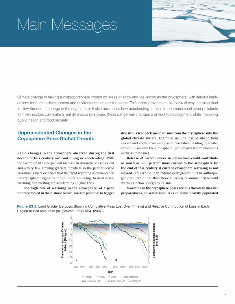
Rapid changes in the cryosphere observed during the first decade of this century are continuing or accelerating. With the exception of a one-percent increase in Antarctic sea ice extent and a very few growing glaciers, nowhere in the peer-reviewed literature is there evidence that the rapid warming documented in the cryosphere beginning in the 1990s is slowing. In most cases, warming and melting are accelerating (Figure ES1).
The high rate of warming in the cryosphere, at a pace unprecedented in the historic record, has the potential to trigger
disastrous feedback mechanisms from the cryosphere into the global climate system. Examples include loss of albedo from sea ice and snow cover and loss of permafrost leading to greater carbon fluxes into the atmosphere (particularly where emissions occur as methane).
Release of carbon stores in permafrost could contribute as much as 5-30 percent more carbon to the atmosphere by the end of this century if current cryosphere warming is not slowed. This would then require even greater cuts in anthropo-genic sources of CO
2 than those currently recommended to hold warming below 2 degrees Celsius.
Warming in the cryosphere poses serious threats to disaster preparedness, to water resources in some heavily populated
Main Messages
Cum
ulat
ive
mea
n sp
ecifi
c m
ass
bala
nce
[103
kg m
2 ]
-10
-5
0
5
-30
-25
-20
-15
-35
Year
1960 2000199019801970 1960 2000199019801970
2
1
0
-1
6
5
4
3
7
Cum
ulat
ive
tota
l mas
s ba
lanc
e [m
m S
LE]
Europe Andes Arctic Asian High Mts.
NW USA+SW-Can. Alaska+Coast Mts. Patagonia
a. b.
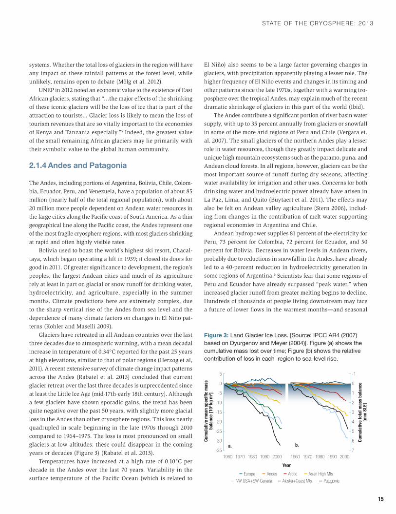
Figure ES 1: Land Glacier Ice Loss, Showing Cumulative Mass Lost Over Time (a) and Relative Contribution of Loss in Each Region to Sea-level Rise (b). (Source: IPCC AR4, (2007.)
On thin ice: hOw cutting pOllutiOn can slOw warming and save lives
2
regions, and to adaptation and ecosystems preservation. Inten-sified monitoring in cryosphere regions is needed to provide better and earlier warning of changes. Monitoring the stability of ice sheets is especially important due to their potential contribu-tion to accelerated worldwide sea-level rise, yet large portions of polar and high alpine regions have few or no observing stations.
Mitigation Strategies in the Cryosphere Have Large and Certain Benefits
Mitigating short-lived climate pollutants (SLCPs), in the com-ing two decades, specifically black carbon and methane can slow these changes while benefiting human communities. Implementing by 2030 the 14 methane and black carbon reduc-tion measures (Table ES1) modeled for this report would bring multiple health, crop, and ecosystems benefits and decrease risks to development from water resource changes, including flooding and other impacts or climate feedbacks we may not foresee today.
Climate benefits for cryosphere regions from black carbon reductions carry less uncertainty than they would in other parts of the globe and are sometimes very large. This is because emissions from sources that emit black carbon—even with other pollutants—almost always lead to warming over reflective ice and snow.
Gains would be eliminated by the end of this century if not accompanied by strong reductions in carbon dioxide (CO
2). Reductions in short-lived climate pollutants cannot be made in isolation from efforts to reduce other greenhouse gases. The role of such reductions is to slow the immediate rate of change, especially in the cryosphere, but cannot replace long-term efforts to reduce CO2.
Certain Sectoral Approaches Offer Tremendous Benefits
Cookstove reduction measures offer by far the greatest poten-tial benefits both to human health and to slowing cryosphere warming. Rapid scaling-up of four existing clean cookstove solu-tions1 could save around one million lives annually2 from outdoor air pollution impacts alone. Current Global Burden of Disease (GBD) estimates place total annual deaths from all household smoke exposure from cookstoves (both outdoor and indoor) at four million annually, greater than the current annual toll from HIV/AIDS, malaria, and tuberculosis combined. Effective sectoral responses, however, would need to deploy models tailored to local and cultural conditions, integrate learning from past failures, be
affordable, and employ best public health practices (including independent monitoring and evaluation).
Cookstove measures delivered climate benefits for all five cryosphere regions modeled,3 including both polar regions; the strongest benefits were in the Himalayas. Fan-assisted biomass cookstoves performed almost as well as biogas/liquefied petroleum gas (LPG) fuel stoves in modeled climate and health benefits (for outdoor exposure), but present challenges to overcome in the field.
Improved biomass (wood) and coal-heating stoves could save about 230,000 lives annually, with the majority of these health benefits occurring in OECD nations.
Just a 50-percent decrease in open field and forest burning could result in around 190,000 fewer deaths annually from related air pollution, making it the second most powerful mea-sure from a health perspective after cookstoves. Human activity causes almost all open field and forest fires, either intentionally or by accident. Effective no-burn alternatives exist for most agri-cultural sector use of fire, and results in this report indicate that up to 90-percent reductions may be possible in some regions.
Reductions in emissions from diesel transport and equip-ment could result in over 16 million tons of additional yield in staple crops such as rice, soy, and wheat, especially in Southeast Asia, as well as averting 340,000 premature deaths. From all measures, including methane measures, the additional increase in crop yield could total nearly 34 million metric tons.
Methane reduction measures primarily target front-end emissions from fossil fuel extraction. While CO2 emissions pri-marily come from fossil fuel use, significant methane and black carbon emissions arise in the production chain for oil, gas, and coal (approximately 65 percent of benefits from all methane measures), strengthening the need for conversion to low-carbon economies.
Reductions Significantly Decrease the Threat of Rapid Cryosphere Change
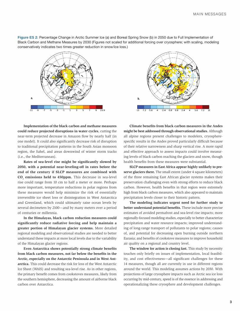
The black carbon and methane measures reviewed could slow warming in the Arctic by more than a full degree by 2050, resulting in up to 40 percent reduced loss of summer sea ice and 25 percent reduced loss of springtime snow cover compared to the baseline (Figure ES2). The Himalayan cryosphere might see nearly a one-degree Celsius decrease from baseline projections (though there is greater uncertainty).
This large decrease in temperature from reduction measures includes the permafrost regions of Siberia, North America, and the Tibetan region, indicating the potential for greater pres-ervation of permafrost regions. This could reduce the risk and extent of future methane and CO
2 releases from permafrost melt.
maIn messaGes
3
Implementation of the black carbon and methane measures could reduce projected disruptions in water cycles, cutting the near-term projected decrease in Amazon flow by nearly half (in one model). It could also significantly decrease risk of disruption to traditional precipitation patterns in the South Asian monsoon region, the Sahel, and areas downwind of winter storm tracks (i.e., the Mediterranean).
Rates of sea-level rise might be significantly slowed by 2050, with a potential near-leveling-off in rates before the end of the century if SLCP measures are combined with CO2 emissions held to 450ppm. This decrease in sea-level rise could range from 10 cm to half a meter or more. Perhaps more important, temperature reductions in polar regions from these measures would help minimize the risk of essentially irreversible ice sheet loss or disintegration in West Antarctica and Greenland, which could ultimately raise ocean levels by several decimeters by 2100—and by many meters over a period of centuries or millennia.
In the Himalayas, black carbon reduction measures could significantly reduce radiative forcing and help maintain a greater portion of Himalayan glacier systems. More detailed regional modeling and observational studies are needed to better understand these impacts at more local levels due to the variability of the Himalayan glacier regions.
Even Antarctica shows potentially strong climate benefits from black carbon measures, not far below the benefits in the Arctic, especially on the Antarctic Peninsula and in West Ant-arctica. This could decrease the risk for loss of the West Antarctic Ice Sheet (WAIS) and resulting sea-level rise. As in other regions, the primary benefit comes from cookstoves measures, likely from the southern hemisphere, decreasing the amount of airborne black carbon over Antarctica.
Climate benefits from black carbon measures in the Andes might be best addressed through observational studies. Although all alpine regions present challenges to modelers, cryosphere-specific results in the Andes proved particularly difficult because of their relative narrowness and sharp vertical rise. A more rapid and effective approach to assess impacts could involve measur-ing levels of black carbon reaching the glaciers and snow, though health benefits from these measures were substantial.
SLCP measures in East Africa appear highly unlikely to pre-serve glaciers there. The small extent (under 4 square kilometers) of the three remaining East African glacier systems makes their preservation challenging even with strong efforts to reduce black carbon. However, health benefits in that region were extremely high from black carbon measures, which also appeared to maintain precipitation levels closer to their historic pattern.
The modeling indicates urgent need for further study to better understand potential benefits. These include more precise estimates of avoided permafrost and sea-level rise impacts; more regionally-focused modeling studies, especially to better characterize precipitation and water resource impacts; improved understand-ing of long-range transport of pollutants to polar regions; causes of, and potential for decreasing open burning outside northern Eurasia; and benefits of cookstove measures to improve household air quality on a regional and country level.
The window for action is closing fast. This study by necessity touches only briefly on issues of implementation, local feasibil-ity, and cost effectiveness—all significant challenges for these 14 measures, though all are currently in use in different regions around the world. This modeling assumes actions by 2030. With projections of large cryosphere impacts such as Arctic sea ice loss occurring by mid-century, speed is of the essence in addressing and operationalizing these cryosphere and development challenges.
Figure ES 2: Percentage Change in Arctic Summer Ice (a) and Boreal Spring Snow (b) in 2050 due to Full Implementation of Black Carbon and Methane Measures by 2030 (Figures not scaled for additional forcing over cryosphere; with scaling, modeling conservatively indicates two times greater reduction in snow/ice loss.)
a. b.
On thin ice: hOw cutting pOllutiOn can slOw warming and save lives
4
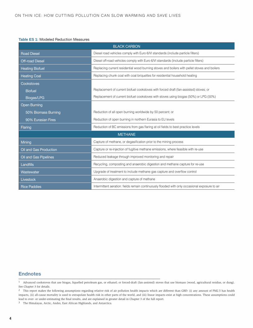
Table ES 1: Modeled Reduction Measures
BLACK CARBON
Road Diesel Diesel road vehicles comply with Euro 6/VI standards (include particle filters)
Off-roadDiesel Diesel off-road vehicles comply with Euro 6/VI standards (include particle filters)
Heating Biofuel replacing current residential wood burning stoves and boilers with pellet stoves and boilers
Heating Coal replacing chunk coal with coal briquettes for residential household heating
CookstovesReplacement of current biofuel cookstoves with forced draft (fan-assisted) stoves; or BiofuelReplacement of current biofuel cookstoves with stoves using biogas (50%) or LPG (50%) Biogas/LPG
Open Burning
50% Biomass Burning Reduction of all open burning worldwide by 50 percent; or
90% Eurasian Fires reduction of open burning in northern eurasia to eU levels
Flaring Reduction of BC emissions from gas flaring at oil fields to best practice levels
METHANE
Mining Capture of methane, or degasification prior to the mining process
Oil and Gas Production Capture or re-injection of fugitive methane emissions, where feasible with re-use
Oil and Gas Pipelines reduced leakage through improved monitoring and repair
Landfills recycling, composting and anaerobic digestion and methane capture for re-use
Wastewater Upgrade of treatment to include methane gas capture and overflow control
Livestock anaerobic digestion and capture of methane
Rice Paddies Intermittent aeration: fields remain continuously flooded with only occasional exposure to air
Endnotes1 Advanced cookstoves that use biogas, liquefied petroleum gas, or ethanol; or forced-draft (fan-assisted) stoves that use biomass (wood, agricultural residue, or dung). See Chapter 3 for details.2 This report makes the following assumptions regarding relative risk of air pollution health impacts which are different than GBD: (i) any amount of PM2.5 has health impacts, (ii) all-cause mortality is used to extrapolate health risk in other parts of the world, and (iii) linear impacts exist at high concentrations. These assumptions could lead to over- or under-estimating the final results, and are explained in greater detail in Chapter 3 of the full report.3 The Himalayas, Arctic, Andes, East African Highlands, and Antarctica.


7
Chapter 1Introduction
Climate change is happening faster and in a dramatically more visible way in the Earth’s cryosphere1 than anywhere else on earth. Global changes in climate are magnified here:
the average temperature has risen at over twice the global mean in the Arctic, Antarctic Peninsula, and much of the Himalayas and other mountain regions, and is well above the global mean in virtually all of the cryosphere around the globe. Not large to begin with, yet providing freshwater to millions in the major urban centers of the Andean nations, the high tropical glaciers of the Andes and Patagonia are disappearing more rapidly perhaps than any others on earth. The glaciers of East Africa have lost 90 percent of their mass in the past century, and today comprise less than four square kilometers in total area.
While the ecosystems and human communities (many of them indigenous) of these regions have felt the impacts of such rapid cryosphere warming most directly, the changes it brings will be felt by billions more, especially in the developing world. The Himalayas store more freshwater ice and snow than any region outside the poles: nearly 10 percent of the global total, directly impacting the water resources of up to 1.5 billion people and providing other services, such as food and electricity, to twice that number (Armstrong 2010). Large populations in Asia rely on the major river systems emanating from the Himalayas, with the Indus and Tarim river systems especially dependent on snow and glacier melt water.
A rise of even one meter in sea level would directly inundate over 100 million people globally (Rowley et al. 2007), with over 50 million in Asia alone; many more would be made susceptible to flooding and tidal surges accompanying hurricanes and typhoons, such as that seen in 2012 in the Philippines (Typhoon Bopha) and northeastern United States (Hurricane Sandy). Small island states and coastal communities in least developed nations face the greatest risks and difficulties in adaptation. The Arctic Council has projected that sea-level rise from glacial melt and other fac-tors likely will exceed one meter in this century (range 0.9–1.5 meters),2 and the recently released Intergovernmental Panel on Climate Change (IPCC) Fifth Assessment Report (AR5)3 placed this range at 0.5–1 meter. Research into the stability of the West
Antarctica Ice Sheet and its role in past sea-level rise indicates it may be an even more important contributor than melting on Greenland; its disintegration ultimately could press these figures even higher (Bamber and Aspinal 2013).
Changes in the cryosphere caused by rapid climate change also have the potential to accelerate climate change globally. When Arctic sea ice disappears to a greater extent each sum-mer, less sunlight is reflected from the northern hemisphere; the darker ocean absorbs heat, warming the entire globe. Similar regional warming occurs due to loss of the albedo effect as high mountain glaciers shrink. Perhaps most serious, both the Arctic and high mountain regions hold large amounts of methane and carbon dioxide (CO
2) in frozen form, from as far back as 400,000 years ago, as permafrost on land and methane hydrates in near-coastal seabeds. As these regions thaw, greenhouse gases will be released into the atmosphere, speeding warming further. Methane in particular is an extremely potent near-term warming agent, and sudden releases could speed warming on a global scale that would be measured in decades.
The fight to preserve cryosphere regions is therefore a global one, with an increasingly short window of opportunity for mean-ingful intervention. Facing a likely loss of summer sea ice by 2030, and disappearance of many land glaciers even earlier, efforts aimed at longer-lived greenhouse gases—while absolutely vital to the long-term preservation of these regions—will not be enough unless accompanied by reductions in more near-term forcers of the regional and global climate systems. Much of the cryosphere is under threat in at most decades, rather than centuries; this threat thus requires measures that will act far more rapidly. This “cryosphere imperative” demands different yet complementary climate solutions to those of the globe as a whole.
Recent and emerging scientific evidence points to the need to address emissions of methane and black carbon, in addition to carbon dioxide, as part of a complementary mix of actions to protect the cryosphere. In addition to reducing the risk of rapid climate change impacts, especially in the developing world, accel-erating actions that reduce these two pollutants, part of the mix known variously as “short lived forcers” or “short-lived climate
On thin ice: hOw cutting pOllutiOn can slOw warming and save lives
8
pollutants”4 can bring immediate and unquestioned health, food security, and other development benefits. Slowing warming in these regions by reducing these pollutants will allow both local and global populations a better chance to adapt and, to the greatest extent possible, mitigate the ongoing ecological changes already occurring in the cryosphere.
This report summarizes the changes already being observed in five major cryosphere regions—the Andes, Antarctica, Arctic, East African Highlands, and the Himalayas with a focus on the most recent research. It then provides a science-based assessment of the impact of addressing methane and black carbon to reduce the risk to the global environment and human societies, especially for the most vulnerable populations.
Chapter 2 provides a comprehensive assessment of the changes occurring in these five regions, based on the most recent literature (including the Fifth Assessment Report (AR5) of the Intergovern-mental Panel on Climate Change (IPCC)). While not included in the scope of this report, similar changes are observed and docu-mented in a wide range of additional cryosphere regions, such as the European Alps and Western Cordillera of North America.
Chapter 3 describes the pollution and climate nexus and the evolving knowledge of how methane and black carbon impact climate specifically in cryosphere regions. Chapter 4 presents the background and methods used for new modeling work conducted as part of this study, which builds extensively on methods used in the 2011 UNEP/WMO Integrated Assessment of Black Carbon and Ozone. Chapter 5 presents the results of the new modeling in these five major cryosphere regions as well as globally for
health, crop impacts, and climate. Finally, Chapter 6 discusses the implications and new directions for the cryosphere regions emerging from these modeling results.
All modeling carries uncertainty, and the climate impact models and health/crop benefit models employed for this study, while peer-reviewed and widely used, are no exception. For example, the global models used have limitations, especially when taken down to more regional levels; the emissions estimates for sources of these pollutants have limitations, especially in developing countries but also worldwide. Furthermore, this report does not aim to address operational feasibility or assess cost effectiveness associated with the emissions reduction scenarios for individual countries or regions within countries. Instead, it is intended as a starting point for work at the local level, taking into account national and local conditions and priorities—but adding the “cryosphere imperative” to the mix. For those wishing to achieve win-win actions on cryosphere and development, this report hopefully can serve as a starting point for exploring these measures, which often have significant local co-benefits, as well as for identifying additional mitigation approaches appropriate to local conditions.
The goal of this report is to give policymakers and other stakeholders an assessment of the current state of the cryosphere and the risks that changes pose to human communities, espe-cially the most vulnerable, and an indication of where acceler-ating certain development and air quality actions that reduce methane and black carbon may bear fruit for both regional and global climate benefits while also directly serving local health and development goals.
Endnotes1 Cryosphere is defined as “elements of the Earth system containing water in its frozen state,” including sea ice, lake and river ice, snow cover and solid precipitation, glaciers, ice caps, ice sheets, ice shelves, permafrost and seasonally frozen ground. 2 Arctic Monitoring and Assessment Program (2011); SWIPA: www.amap.no.3 IPCC Working Group I Report (Sept. 27, 2013).4 This report uses these different terms interchangeably to refer to black carbon and methane, including impacts on ozone (considered another short-lived forcer or climate pollutant) from methane and black carbon reductions.


11
Chapter 2State of the Cryosphere: 2013
As the most rapidly warming regions on earth, the cryo-sphere has variously been characterized as the canary in the coalmine, an early-warning signal, or a sign of
things to come. It is all these things—and those changes have global implications.
A number of excellent summaries of cryosphere climate change were published in 2008–09, especially associated with the conclusion of the International Polar Year.1 This section seeks to update developments since then in five major cryosphere regions of the globe: the alpine ecosystems of the Himalayas, Andes and East African Highlands, and the Arctic and Antarctic at the Poles. It summarizes the latest developments in processes that cut across these different regions: loss of albedo through melt-ing and exposure of rock, soil, or open water; sea-level rise from melting of land glaciers and ice caps; and loss of permafrost. All three processes could lead to feedback mechanisms that speed warming and have serious consequences for the global climate system, with repercussions for the environment, biodiversity, and human society.
2.1 Climate Change Impacts in Five Cryosphere Regions
2.1.1 The Himalayas
The Himalayan mountain ranges—extending 2,400 km through six nations (India, Pakistan, Afghanistan, China, Bhutan, and Nepal)—make up the largest cryosphere region and fresh water source outside the poles. Rapid climate-induced changes in the region directly affect the water resources of more than 1.5 billion lives, as well as services such as electricity, and the food supplies of 3 billion. Projected and observed impacts include disruption of the annual monsoon, changes in runoff from river basins, and an increased risk of flooding and landslides (see Figure 1).
Annual mean surface temperature across the Himalayan region has increased by 1.5ºC 2 over pre-industrial average
temperatures—similar to increases seen in the Arctic and Antarctic Peninsula (Shrestha, Gautam, and Bawa 2012). Measuring the impacts of this temperature rise on the Himalayan cryosphere has proved challenging because of the complicated topography that makes each glacier and region unique and difficult to study, even using satellite technology (Fujita and Nuimura 2011).
Despite the complexity of observations and the lack of on-site measurements, an overall pattern of warming and melting has been apparent, with evidence of glacier and snow cover decrease recorded across most of the Himalayan region (Bolch et al. 2012; Armstrong 2010; Bamber 2012; Kang et al. 2010). The most extreme melting has occurred in the eastern Himalayas, where the mean glacial thickness of Chinese glaciers decreased by nearly 11 meters from 1985–2005. A more mixed pattern is evident in the far Northwest and the Karakoram region, which are further north, colder, and more remote from large human populations and from monsoon precipitation impacts, receiving greater humidity from the west and the winter monsoon season (UNEP-GRID 2012; Kaab 2012; Yao et al. 2012).
Many glacial lakes have formed or expanded during the rapid melt process in the Eastern and Central Himalayas. These have led to catastrophic floods—so-called glacial lake outbursts (GLOFs)—especially in Nepal and the Tibetan region. Other GLOFs have been narrowly averted there and in Bhutan by implement-ing measures such as siphoning off melt water, as occurred with Tsho Rolpa in Nepal (Liu et al. 2013).
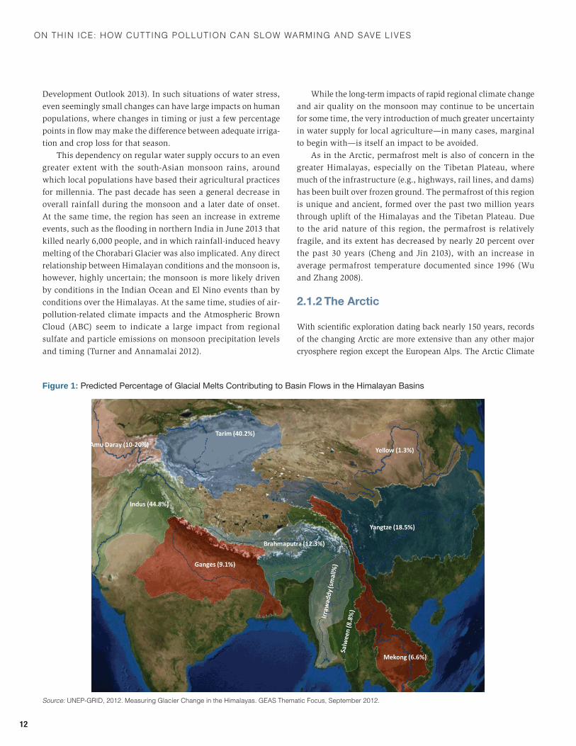
The importance of melt water from greater Himalayan glaciers and snowpack to human water supplies varies widely, with the semi-arid regions of western China, Pakistan and Central Asia most clearly dependent on a regular, predictable melt season (Immerzeel, van Beek, and Bierkens 2010). Estimates range from 80-percent dependency of overall river flow on melt water in these western regions (especially the Indus and Tarim river basins) to under 20 percent in the Yangtze, Ganges, and Yellow Rivers (see Figure 1) (Xu, Shrestha, and Eriksson 2009). A 2013 report by the Asian Development Bank categorized Pakistan as one of the most water-stressed nations in the world, largely due to changes already seen in the supply to the Indus River (Asian
On thin ice: hOw cutting pOllutiOn can slOw warming and save lives
12
Development Outlook 2013). In such situations of water stress, even seemingly small changes can have large impacts on human populations, where changes in timing or just a few percentage points in flow may make the difference between adequate irriga-tion and crop loss for that season.
This dependency on regular water supply occurs to an even greater extent with the south-Asian monsoon rains, around which local populations have based their agricultural practices for millennia. The past decade has seen a general decrease in overall rainfall during the monsoon and a later date of onset. At the same time, the region has seen an increase in extreme events, such as the flooding in northern India in June 2013 that killed nearly 6,000 people, and in which rainfall-induced heavy melting of the Chorabari Glacier was also implicated. Any direct relationship between Himalayan conditions and the monsoon is, however, highly uncertain; the monsoon is more likely driven by conditions in the Indian Ocean and El Nino events than by conditions over the Himalayas. At the same time, studies of air-pollution-related climate impacts and the Atmospheric Brown Cloud (ABC) seem to indicate a large impact from regional sulfate and particle emissions on monsoon precipitation levels and timing (Turner and Annamalai 2012).
While the long-term impacts of rapid regional climate change and air quality on the monsoon may continue to be uncertain for some time, the very introduction of much greater uncertainty in water supply for local agriculture—in many cases, marginal to begin with—is itself an impact to be avoided.
As in the Arctic, permafrost melt is also of concern in the greater Himalayas, especially on the Tibetan Plateau, where much of the infrastructure (e.g., highways, rail lines, and dams) has been built over frozen ground. The permafrost of this region is unique and ancient, formed over the past two million years through uplift of the Himalayas and the Tibetan Plateau. Due to the arid nature of this region, the permafrost is relatively fragile, and its extent has decreased by nearly 20 percent over the past 30 years (Cheng and Jin 2103), with an increase in average permafrost temperature documented since 1996 (Wu and Zhang 2008).
2.1.2 The Arctic
With scientific exploration dating back nearly 150 years, records of the changing Arctic are more extensive than any other major cryosphere region except the European Alps. The Arctic Climate
Figure 1: Predicted Percentage of Glacial Melts Contributing to Basin Flows in the Himalayan Basins
Source: UneP-GrId, 2012. measuring Glacier Change in the himalayas. Geas thematic focus, september 2012.
state of the CryosPhere: 2013
13
Impact Assessment (ACIA) report of the Arctic Council in 2004 comprised the first comprehensive assessment of climate change in the Arctic, and delivered a dramatic message to the world on the changes already occurring there. The Council expanded this work in the 2011 Snow, Water, Ice, and Permafrost in the Arctic (SWIPA) report.3
A key finding from SWIPA was that observed changes in the Arctic had far outpaced any projections from scientific model-ing, with loss of sea ice, glaciers, snow cover, and permafrost occurring at rates far more rapid than even the most pessimistic IPCC modeling scenarios. This pace of change has continued, and includes the following recent developments.
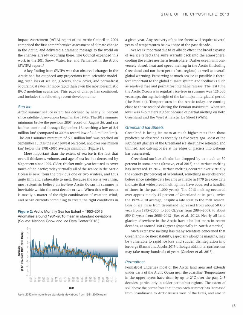
Sea IceArctic summer sea ice extent has declined by nearly 50 percent since satellite observations began in the 1970s. The 2012 summer minimum broke the previous 2007 record on August 26, and sea ice loss continued through September 16, reaching a low of 3.4 million km2 (compared to 2007’s record low of 4.2 million km2). The 2013 summer minimum of 5.1 million km2 was reached on September 13; it is the sixth lowest on record, and over one million km2 below the 1981–2010 average minimum (Figure 2).
More important than the extent of sea ice is the fact that overall thickness, volume, and age of sea ice has decreased by 80 percent since 1979. Older, thicker multi-year ice used to cover much of the Arctic; today virtually all of the sea ice in the Arctic Ocean is new, from the previous one or two winters, and thus quite thin and vulnerable to melt. Because the ice is very thin, most scientists believe an ice-free Arctic Ocean in summer is inevitable within the next decade or two. When this will occur is mostly a matter of the right combination of weather, wind, and ocean currents combining to create the right conditions in
a given year. Any recovery of the ice sheets will require several years of temperatures below those of the past decade.
Sea ice is important due to its albedo effect: the broad expanse of sea ice reflects the sun’s warmth back into the atmosphere, cooling the entire northern hemisphere. Darker ocean will con-versely absorb heat and speed melting in the Arctic (including Greenland and northern permafrost regions) as well as overall global warming. Preserving as much sea ice as possible is there-fore important to the global climate system and feedbacks such as sea-level rise and permafrost methane release. The last time the Arctic Ocean was regularly ice-free in summer was 125,000 years ago, during the height of the last major interglacial period (the Eemian). Temperatures in the Arctic today are coming close to those reached during the Eemian maximum, when sea level was 4–6 meters higher because of partial melting on both Greenland and the West Antarctic Ice Sheet (WAIS).
Greenland Ice SheetsGreenland is losing ice mass at much higher rates than those predicted or observed as recently as five years ago. Most of the significant glaciers of the Greenland ice sheet have retreated and thinned, and calving of ice at the edges of glaciers into icebergs has accelerated.
Greenland surface albedo has dropped by as much as 30 percent in some areas (Stroeve, et al 2013) and surface melting has increased. In 2012, surface melting occurred over virtually the entirety (97 percent) of Greenland, something never observed before since satellite data became available in 1979 (ice core data indicate that widespread melting may have occurred a handful of times in the past 1,000 years). The 2013 melting occurred over approximately 45 percent of Greenland at its peak, twice the 1979–2010 average, despite a late start to the melt season. Loss of ice mass from Greenland increased from about 50 Gt/year from 1995–2000, to 200 Gt/year from 2004–2008, to about 350 Gt/year from 2008–2012 (Box et al. 2012). Nearly all land glaciers elsewhere in the Arctic have also lost mass in recent decades, at around 150 Gt/year (especially in North America).
Such extensive melting has many scientists concerned that Greenland’s ice sheet stability, especially along the margins, may be vulnerable to rapid ice loss and sudden disintegration into icebergs (Bassis and Jacobs 2013), though additional surface loss may take many hundreds of years (Goelzer et al. 2013).
PermafrostPermafrost underlies most of the Arctic land area and extends under parts of the Arctic Ocean near the coastline. Temperatures in the upper layers have risen by up to 2°C over the past 2–3 decades, particularly in colder permafrost regions. The extent of soil above the permafrost that thaws each summer has increased from Scandinavia to Arctic Russia west of the Urals, and also in
Figure 2: Arctic Monthly Sea Ice Extent – 1953–2013 Anomalies around 1981–2010 mean in standard deviations. (Source: National Snow and Ice Data Center 2013.)
Note: 2012 minimum three standards deviations from 1981-2010 mean.
Anom
aly
(# S
t. De
v. fr
om 1
981-
2010
Mea
n)
3
4
5
6
-1
0
1
2
-3
-4
-2
1953
1956
1959
1962
1965
1968
1971
1974
1977
1980
1983
1986
1989
1992
1995
1998
2001
2004
2007
2010
2013
Year
On thin ice: hOw cutting pOllutiOn can slOw warming and save lives
14
Alaska. The southern limit of permafrost in Russia has moved northwards by 30–80 km during the same period; and by 130 km in Quebec during the last 50 years. Summer icebreaker expedi-tions over the past three years have documented large volumes of methane gas bubbling to the surface off the Siberian coastline.
The amount of carbon held in Arctic permafrost remains uncertain, but most scientists estimate that it at least equals the amount of carbon released from anthropogenic sources since pre-industrial times. Methane raises particular concern: SWIPA estimated that a release of just 1 percent of the methane present in permafrost below the seabed of the East Siberian shelf would have a warming effect equivalent to a doubling of the amount of carbon dioxide in the atmosphere. Holding temperatures as low as possible in Arctic permafrost is therefore an issue of global concern.
AcidificationThe Arctic Ocean is particularly sensitive to acidification, because increasing amounts of fresh water entering the Arctic Ocean from rivers and melting ice are reducing the Arctic’s capacity to neu-tralize acidification. Widespread acidification has already been observed in the central Arctic Ocean and has been documented at monitoring sites across the region, especially in surface waters. Because Arctic marine food webs are relatively simple, its eco-systems are vulnerable to change when key species are affected (Shadwick et al. 2013).
The Arctic and surrounding waters contain the largest fish-ing waters of the northern hemisphere, resources already under stress from historical overfishing and other environmental stresses. Increasing acidification may also impact these com-mercial fisheries as well as marine resources that are used by Arctic indigenous people.4
2.1.3 East African Highlands
Most people do not associate Africa with cryosphere regions, yet the East African Highlands may have contained glaciers since the last glacier maximum 11,000 years ago. Seasonal cryosphere, in the form of snow, exists on the highest peaks of East Africa as well as in the Drakensburg Range of South Africa, the Lesotho Mountains, and the Atlas Mountains in Morocco. The only exist-ing African glaciers today are on Mt. Kilimanjaro, Mt. Kenya, and three glacier systems in the Rwenzori (“Mountains of the Moon”) between Uganda and the Democratic Republic of Congo. These glaciers likely covered around 25 km2 in total in the early 1900s; today they cover well under 4 km2, based on the most recent surveys (tracking of the Rwenzori is especially difficult, even by satellite) (Mölg et al. 2013; UNEP 2013).
The Rwenzori in 1906 contained 43 named glaciers, distributed across six peaks and estimated to be half of the glacial area in
East Africa at the time (Taylor et al. 2006). At its maximum dur-ing the last glacial period, the Kilimanjaro ice sheet covered over 400 km2 (Young and Hastenwrath 1987). By 1912, when reliable observations began, Kilimanjaro’s glacier extent was 11.4 km2. It had diminished to 1.8 km2 in 2011, losing nearly 90 percent of its extent over 100 years; this includes nearly 30 percent loss of the ice extent that was present in 2000 (Thompson et al. 2009; Cullen et al. 2002). The latest estimates of Rwenzori are under 2 km2, and Mt. Kenya has retreated to about 0.1 km2. These glaciers therefore are among the most rapidly receding in the world, losing between 80–90 percent of their surface area since observations began in the late 1800s. Few glaciologists expect these glaciers to survive past 2050, and some estimate a disappearance by 2030.
The connection between the retreat of these glaciers and anthropogenic climate change is very complex, as is the climate of East Africa generally. Influences on the region arise from processes ranging from the Indian Ocean and seasonal monsoon (itself tied to El Nino) to winds off the Sahara and even from Antarctica. Extensive research on Kilimanjaro indicates that a variety of factors, including changes in precipitation patterns and dryness in the region, seem the greatest factors contribut-ing to glacial melt there over the past few decades (Mölg et al. 2009). The role of temperature remains an area of active debate among tropical glaciologists, with different processes potentially contributing more or less to the different glaciers (Kaser et al. 2004), and Kilimanjaro being perhaps an especially unique case (Mölg, et al. 2010).
Although the processes causing these shifts remain an area of debate, tropical glaciologists do broadly agree that climate change has impacted the rate of observed glacial loss in East Africa in the past few decades (Mölg, et al. 2010). Summit ice cover on Kilimanjaro decreased by about one percent per year from 1912–1953, but had risen to 2.5 percent per year from 1989–2007. Ice core studies on Kilimanjaro show clear evidence of surface glacier melt only in the upper 65 cm of the 49-meter core that spans around 11,000 years. This may indicate that the climate conditions driving the loss of Kilimanjaro’s ice fields are relatively recent (Thompson, et al. 2009).
This region has generated some debate as to the impact of climate change on the spread of malaria, since the temperature-sensitive mosquito that carries the disease had been observed higher in East African mountain communities a decade ago. The spread of malaria in the late 1990s probably was caused by other factors; yet the mosquito’s range can increase as temperature rises, and local communities remain vigilant (Stern et al. 2011).
Glacier and snow melt form a very small portion of water resources in this region, with recent measurements showing them contributing at 2 percent or less (Taylor et al. 2009). The rain forests along the sides of these peaks, and rainfall at those altitudes play the greatest role in East African water resource
state of the CryosPhere: 2013
15
systems. Whether the total loss of glaciers in the region will have any impact on these rainfall patterns at the forest level, while unlikely, remains open to debate (Mölg et al. 2012).
UNEP in 2012 noted an economic value to the existence of East African glaciers, stating that “…the major effects of the shrinking of these iconic glaciers will be the loss of ice that is part of the attraction to tourists... Glacier loss is likely to mean the loss of tourism revenues that are so vitally important to the economies of Kenya and Tanzania especially.”5 Indeed, the greatest value of the small remaining African glaciers may lie primarily with their symbolic value to the global human community.
2.1.4 Andes and Patagonia
The Andes, including portions of Argentina, Bolivia, Chile, Colom-bia, Ecuador, Peru, and Venezuela, have a population of about 85 million (nearly half of the total regional population), with about 20 million more people dependent on Andean water resources in the large cities along the Pacific coast of South America. As a thin geographical line along the Pacific coast, the Andes represent one of the most fragile cryosphere regions, with most glaciers shrinking at rapid and often highly visible rates.
Bolivia used to boast the world’s highest ski resort, Chacal-taya, which began operating a lift in 1939; it closed its doors for good in 2011. Of greater significance to development, the region’s peoples, the largest Andean cities and much of its agriculture rely at least in part on glacial or snow runoff for drinking water, hydroelectricity, and agriculture, especially in the summer months. Climate predictions here are extremely complex, due to the sharp vertical rise of the Andes from sea level and the dependence of many climate factors on changes in El Niño pat-terns (Kohler and Maselli 2009).
Glaciers have retreated in all Andean countries over the last three decades due to atmospheric warming, with a mean decadal increase in temperature of 0.34°C reported for the past 25 years at high elevations, similar to that of polar regions (Herzog et al, 2011). A recent extensive survey of climate change impact patterns across the Andes (Rabatel et al. 2013) concluded that current glacier retreat over the last three decades is unprecedented since at least the Little Ice Age (mid-17th-early 18th century). Although a few glaciers have shown sporadic gains, the trend has been quite negative over the past 50 years, with slightly more glacial loss in the Andes than other cryosphere regions. This loss nearly quadrupled in scale beginning in the late 1970s through 2010 compared to 1964–1975. The loss is most pronounced on small glaciers at low altitudes: these could disappear in the coming years or decades (Figure 3) (Rabatel et al. 2013).
Temperatures have increased at a high rate of 0.10°C per decade in the Andes over the last 70 years. Variability in the surface temperature of the Pacific Ocean (which is related to
El Niño) also seems to be a large factor governing changes in glaciers, with precipitation apparently playing a lesser role. The higher frequency of El Niño events and changes in its timing and other patterns since the late 1970s, together with a warming tro-posphere over the tropical Andes, may explain much of the recent dramatic shrinkage of glaciers in this part of the world (Ibid).
The Andes contribute a significant portion of river basin water supply, with up to 35 percent annually from glaciers or snowfall in some of the more arid regions of Peru and Chile (Vergara et. al. 2007). The small glaciers of the northern Andes play a lesser role in water resources, though they greatly impact delicate and unique high mountain ecosystems such as the paramo, puna, and Andean cloud forests. In all regions, however, glaciers can be the most important source of runoff during dry seasons, affecting water availability for irrigation and other uses. Concerns for both drinking water and hydroelectric power already have arisen in La Paz, Lima, and Quito (Buytaert et al. 2011). The effects may also be felt on Andean valley agriculture (Stern 2006), includ-ing from changes in the contribution of melt water supporting regional economies in Argentina and Chile.
Andean hydropower supplies 81 percent of the electricity for Peru, 73 percent for Colombia, 72 percent for Ecuador, and 50 percent for Bolivia. Decreases in water levels in Andean rivers, probably due to reductions in snowfall in the Andes, have already led to a 40-percent reduction in hydroelectricity generation in some regions of Argentina.6 Scientists fear that some regions of Peru and Ecuador have already surpassed “peak water,” when increased glacier runoff from greater melting begins to decline. Hundreds of thousands of people living downstream may face a future of lower flows in the warmest months—and seasonal
Figure 3: Land Glacier Ice Loss. [Source: IPCC AR4 (2007) based on Dyurgenov and Meyer (2004)]. Figure (a) shows the cumulative mass lost over time; Figure (b) shows the relative contribution of loss in each region to sea-level rise.
Cum
ulat
ive
mea
n sp
ecifi
c m
ass
bala
nce
[103
kg m
2 ]
-10
-5
0
5
-30
-25
-20
-15
-35
Year
1960 2000199019801970 1960 2000199019801970
2
1
0
-1
6
5
4
3
7
Cum
ulat
ive
tota
l mas
s ba
lanc
e [m
m S
LE]
Europe Andes Arctic Asian High Mts.
NW USA+SW-Canada Alaska+Coast Mts. Patagonia
a. b.
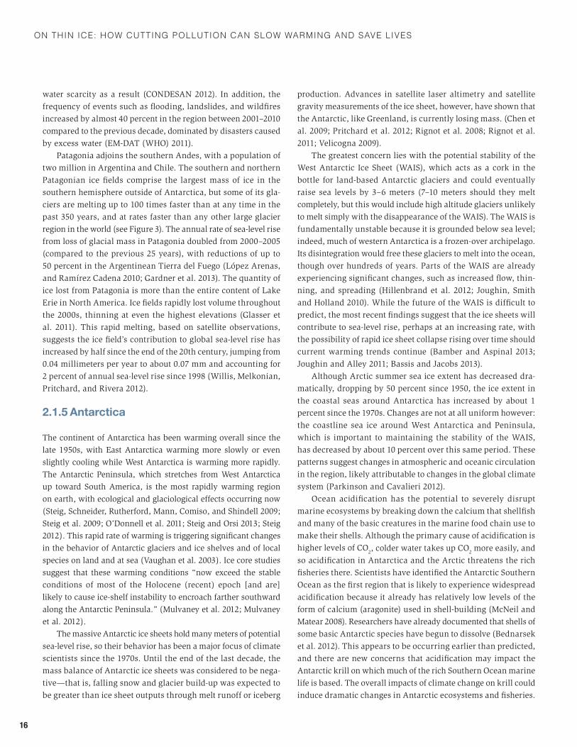
On thin ice: hOw cutting pOllutiOn can slOw warming and save lives
16
water scarcity as a result (CONDESAN 2012). In addition, the frequency of events such as flooding, landslides, and wildfires increased by almost 40 percent in the region between 2001–2010 compared to the previous decade, dominated by disasters caused by excess water (EM-DAT (WHO) 2011).
Patagonia adjoins the southern Andes, with a population of two million in Argentina and Chile. The southern and northern Patagonian ice fields comprise the largest mass of ice in the southern hemisphere outside of Antarctica, but some of its gla-ciers are melting up to 100 times faster than at any time in the past 350 years, and at rates faster than any other large glacier region in the world (see Figure 3). The annual rate of sea-level rise from loss of glacial mass in Patagonia doubled from 2000–2005 (compared to the previous 25 years), with reductions of up to 50 percent in the Argentinean Tierra del Fuego (López Arenas, and Ramírez Cadena 2010; Gardner et al. 2013). The quantity of ice lost from Patagonia is more than the entire content of Lake Erie in North America. Ice fields rapidly lost volume throughout the 2000s, thinning at even the highest elevations (Glasser et al. 2011). This rapid melting, based on satellite observations, suggests the ice field’s contribution to global sea-level rise has increased by half since the end of the 20th century, jumping from 0.04 millimeters per year to about 0.07 mm and accounting for 2 percent of annual sea-level rise since 1998 (Willis, Melkonian, Pritchard, and Rivera 2012).
2.1.5 Antarctica
The continent of Antarctica has been warming overall since the late 1950s, with East Antarctica warming more slowly or even slightly cooling while West Antarctica is warming more rapidly. The Antarctic Peninsula, which stretches from West Antarctica up toward South America, is the most rapidly warming region on earth, with ecological and glaciological effects occurring now (Steig, Schneider, Rutherford, Mann, Comiso, and Shindell 2009; Steig et al. 2009; O’Donnell et al. 2011; Steig and Orsi 2013; Steig 2012). This rapid rate of warming is triggering significant changes in the behavior of Antarctic glaciers and ice shelves and of local species on land and at sea (Vaughan et al. 2003). Ice core studies suggest that these warming conditions “now exceed the stable conditions of most of the Holocene (recent) epoch [and are] likely to cause ice-shelf instability to encroach farther southward along the Antarctic Peninsula.” (Mulvaney et al. 2012; Mulvaney et al. 2012).
The massive Antarctic ice sheets hold many meters of potential sea-level rise, so their behavior has been a major focus of climate scientists since the 1970s. Until the end of the last decade, the mass balance of Antarctic ice sheets was considered to be nega-tive—that is, falling snow and glacier build-up was expected to be greater than ice sheet outputs through melt runoff or iceberg
production. Advances in satellite laser altimetry and satellite gravity measurements of the ice sheet, however, have shown that the Antarctic, like Greenland, is currently losing mass. (Chen et al. 2009; Pritchard et al. 2012; Rignot et al. 2008; Rignot et al. 2011; Velicogna 2009).
The greatest concern lies with the potential stability of the West Antarctic Ice Sheet (WAIS), which acts as a cork in the bottle for land-based Antarctic glaciers and could eventually raise sea levels by 3–6 meters (7–10 meters should they melt completely, but this would include high altitude glaciers unlikely to melt simply with the disappearance of the WAIS). The WAIS is fundamentally unstable because it is grounded below sea level; indeed, much of western Antarctica is a frozen-over archipelago. Its disintegration would free these glaciers to melt into the ocean, though over hundreds of years. Parts of the WAIS are already experiencing significant changes, such as increased flow, thin-ning, and spreading (Hillenbrand et al. 2012; Joughin, Smith and Holland 2010). While the future of the WAIS is difficult to predict, the most recent findings suggest that the ice sheets will contribute to sea-level rise, perhaps at an increasing rate, with the possibility of rapid ice sheet collapse rising over time should current warming trends continue (Bamber and Aspinal 2013; Joughin and Alley 2011; Bassis and Jacobs 2013).
Although Arctic summer sea ice extent has decreased dra-matically, dropping by 50 percent since 1950, the ice extent in the coastal seas around Antarctica has increased by about 1 percent since the 1970s. Changes are not at all uniform however: the coastline sea ice around West Antarctica and Peninsula, which is important to maintaining the stability of the WAIS, has decreased by about 10 percent over this same period. These patterns suggest changes in atmospheric and oceanic circulation in the region, likely attributable to changes in the global climate system (Parkinson and Cavalieri 2012).
Ocean acidification has the potential to severely disrupt marine ecosystems by breaking down the calcium that shellfish and many of the basic creatures in the marine food chain use to make their shells. Although the primary cause of acidification is higher levels of CO
2, colder water takes up CO2 more easily, and so acidification in Antarctica and the Arctic threatens the rich fisheries there. Scientists have identified the Antarctic Southern Ocean as the first region that is likely to experience widespread acidification because it already has relatively low levels of the form of calcium (aragonite) used in shell-building (McNeil and Matear 2008). Researchers have already documented that shells of some basic Antarctic species have begun to dissolve (Bednarsek et al. 2012). This appears to be occurring earlier than predicted, and there are new concerns that acidification may impact the Antarctic krill on which much of the rich Southern Ocean marine life is based. The overall impacts of climate change on krill could induce dramatic changes in Antarctic ecosystems and fisheries.
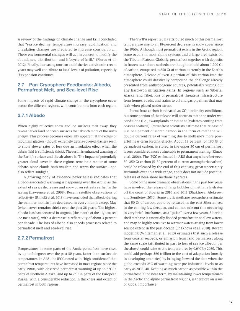
state of the CryosPhere: 2013
17
A review of the findings on climate change and krill concluded that “sea ice decline, temperature increase, acidification, and circulation changes are predicted to increase considerably… These environmental changes will act in concert to modify the abundance, distribution, and lifecycle of krill.” (Flores et al. 2012). Finally, increasing tourism and fisheries activities in recent years may well contribute to local levels of pollution, especially if expansion continues.
2.7 Pan-Cryosphere Feedbacks: Albedo, Permafrost Melt, and Sea-level Rise
Some impacts of rapid climate change in the cryosphere occur across the different regions, with contributions from each region.
2.7.1 Albedo
When highly reflective snow and ice surfaces melt away, they reveal darker land or ocean surfaces that absorb more of the sun’s energy. This process becomes especially apparent at the edges of mountain glaciers (though extremely debris-covered glaciers seem to show slower rates of loss due an insulation effect when the debris field is sufficiently thick). The result is enhanced warming of the Earth’s surface and the air above it. The impact of potentially greater cloud cover in these regions remains a matter of some debate, since clouds both insulate and warm the surface—and also reflect sunlight.
A growing body of evidence nevertheless indicates that albedo-associated warming is happening over the Arctic as the extent of sea ice decreases and snow cover retreats earlier in the spring (Lawrence et al. 2008). Recent satellite observations of reflectivity (Riihelä et al. 2013) have concluded that albedo during the summer months has decreased in every month except May (when cover remains thick) over the past 28 years. The highest albedo loss has occurred in August, (the month of the highest sea ice melt rates), with a decrease in reflectivity of about 3 percent per decade. The loss of albedo also speeds processes related to permafrost melt and sea-level rise.
2.7.2 Permafrost
Temperatures in some parts of the Arctic permafrost have risen by up to 2 degrees over the past 30 years, faster than surface air temperatures. In AR5, the IPCC noted with “high confidence” that permafrost temperatures have increased in most regions since the early 1980s, with observed permafrost warming of up to 3°C in parts of Northern Alaska, and up to 2°C in parts of the European Russia, with a considerable reduction in thickness and extent of permafrost in both regions.
The SWIPA report (2011) attributed much of this permafrost temperature rise to an 18-percent decrease in snow cover since the 1960s. Although most permafrost exists in the Arctic region, some occurs in most alpine systems and a large area exists on the Tibetan Plateau. Globally, permafrost together with deposits in frozen near-shore seabeds are thought to hold about 1,700 Gt of carbon, compared to 850 Gt of carbon currently in the Earth’s atmosphere. Release of even a portion of this carbon into the atmosphere could drastically compound the challenge already presented from anthropogenic sources, potentially wiping out any hard-won mitigation gains. In regions such as Siberia, Alaska, and Tibet, loss of permafrost threatens infrastructure from homes, roads, and trains to oil and gas pipelines that may leak when placed under stress.
Permafrost carbon is released as CO2 under dry conditions,
but some portion of the release will occur as methane under wet conditions (i.e., swamplands or methane hydrates coming from coastal seabeds). Permafrost scientists estimate that release of just one percent of stored carbon in the form of methane will double current rates of warming due to methane’s more pow-erful near-term forcing effects. About 12 percent, or 190 Gt of permafrost carbon, is stored in the upper 30 cm of permafrost layers considered most vulnerable to permanent melting (Zimov et al. 2006). The IPCC estimated in AR5 that anywhere between 50–250 Gt carbon (5–30 percent of current atmospheric carbon) could be released by the end of this century; great uncertainty surrounds even this wide range, and it does not include potential releases of near-shore methane hydrates.
Some of the more dramatic observations in the past few years have involved the release of large bubbles of methane hydrates off the coast of Siberia in 2010 and 2011 (Shakhova, Alekseev, and Semiletov, 2010). Some arctic methane researchers estimate that 50 Gt of carbon could be released in the east Siberian sea in the coming few decades, and cannot rule out this occurring in very brief timeframes, as a “pulse” over a few years. Siberian shelf methane is essentially flooded permafrost in shallow waters, and may be highly sensitive to warmer waters arising from lower sea ice extent in the past decade (Shakhova et al. 2010). Recent modeling (Whiteman et al. 2013) estimates that such a release from coastal seabeds, or emission from land permafrost along the same scale (attributed in part to loss of sea ice albedo, per the above) could raise Arctic temperatures by 0.6°C by 2050. This could add perhaps $60 trillion to the cost of adaptation (mostly in developing countries) by bringing forward the date when the globe exceeds 2°C of warming over pre-industrial levels to as early as 2035–40. Keeping as much carbon as possible within the permafrost in the near-term, by maintaining lower temperatures in the Arctic and alpine permafrost regions, is therefore an issue of global importance.
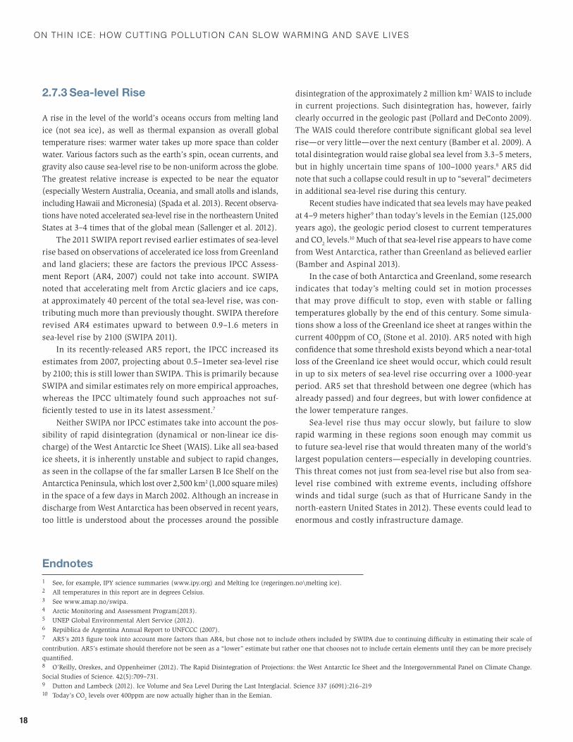
On thin ice: hOw cutting pOllutiOn can slOw warming and save lives
18
2.7.3 Sea-level Rise
A rise in the level of the world’s oceans occurs from melting land ice (not sea ice), as well as thermal expansion as overall global temperature rises: warmer water takes up more space than colder water. Various factors such as the earth’s spin, ocean currents, and gravity also cause sea-level rise to be non-uniform across the globe. The greatest relative increase is expected to be near the equator (especially Western Australia, Oceania, and small atolls and islands, including Hawaii and Micronesia) (Spada et al. 2013). Recent observa-tions have noted accelerated sea-level rise in the northeastern United States at 3–4 times that of the global mean (Sallenger et al. 2012).
The 2011 SWIPA report revised earlier estimates of sea-level rise based on observations of accelerated ice loss from Greenland and land glaciers; these are factors the previous IPCC Assess-ment Report (AR4, 2007) could not take into account. SWIPA noted that accelerating melt from Arctic glaciers and ice caps, at approximately 40 percent of the total sea-level rise, was con-tributing much more than previously thought. SWIPA therefore revised AR4 estimates upward to between 0.9–1.6 meters in sea-level rise by 2100 (SWIPA 2011).
In its recently-released AR5 report, the IPCC increased its estimates from 2007, projecting about 0.5–1meter sea-level rise by 2100; this is still lower than SWIPA. This is primarily because SWIPA and similar estimates rely on more empirical approaches, whereas the IPCC ultimately found such approaches not suf-ficiently tested to use in its latest assessment.7
Neither SWIPA nor IPCC estimates take into account the pos-sibility of rapid disintegration (dynamical or non-linear ice dis-charge) of the West Antarctic Ice Sheet (WAIS). Like all sea-based ice sheets, it is inherently unstable and subject to rapid changes, as seen in the collapse of the far smaller Larsen B Ice Shelf on the Antarctica Peninsula, which lost over 2,500 km2 (1,000 square miles) in the space of a few days in March 2002. Although an increase in discharge from West Antarctica has been observed in recent years, too little is understood about the processes around the possible
disintegration of the approximately 2 million km2 WAIS to include in current projections. Such disintegration has, however, fairly clearly occurred in the geologic past (Pollard and DeConto 2009). The WAIS could therefore contribute significant global sea level rise—or very little—over the next century (Bamber et al. 2009). A total disintegration would raise global sea level from 3.3–5 meters, but in highly uncertain time spans of 100–1000 years.8 AR5 did note that such a collapse could result in up to “several” decimeters in additional sea-level rise during this century.
Recent studies have indicated that sea levels may have peaked at 4–9 meters higher9 than today’s levels in the Eemian (125,000 years ago), the geologic period closest to current temperatures and CO2 levels.10 Much of that sea-level rise appears to have come from West Antarctica, rather than Greenland as believed earlier (Bamber and Aspinal 2013).
In the case of both Antarctica and Greenland, some research indicates that today’s melting could set in motion processes that may prove difficult to stop, even with stable or falling temperatures globally by the end of this century. Some simula-tions show a loss of the Greenland ice sheet at ranges within the current 400ppm of CO2 (Stone et al. 2010). AR5 noted with high confidence that some threshold exists beyond which a near-total loss of the Greenland ice sheet would occur, which could result in up to six meters of sea-level rise occurring over a 1000-year period. AR5 set that threshold between one degree (which has already passed) and four degrees, but with lower confidence at the lower temperature ranges.
Sea-level rise thus may occur slowly, but failure to slow rapid warming in these regions soon enough may commit us to future sea-level rise that would threaten many of the world’s largest population centers—especially in developing countries. This threat comes not just from sea-level rise but also from sea-level rise combined with extreme events, including offshore winds and tidal surge (such as that of Hurricane Sandy in the north-eastern United States in 2012). These events could lead to enormous and costly infrastructure damage.
Endnotes1 See, for example, IPY science summaries (www.ipy.org) and Melting Ice (regeringen.no\melting ice). 2 All temperatures in this report are in degrees Celsius.3 See www.amap.no/swipa.4 Arctic Monitoring and Assessment Program(2013). 5 UNEP Global Environmental Alert Service (2012). 6 República de Argentina Annual Report to UNFCCC (2007).7 AR5’s 2013 figure took into account more factors than AR4, but chose not to include others included by SWIPA due to continuing difficulty in estimating their scale of contribution. AR5’s estimate should therefore not be seen as a “lower” estimate but rather one that chooses not to include certain elements until they can be more precisely quantified.8 O’Reilly, Oreskes, and Oppenheimer (2012). The Rapid Disintegration of Projections: the West Antarctic Ice Sheet and the Intergovernmental Panel on Climate Change. Social Studies of Science. 42(5):709–731.9 Dutton and Lambeck (2012). Ice Volume and Sea Level During the Last Interglacial. Science 337 (6091):216–219 10 Today’s CO2 levels over 400ppm are now actually higher than in the Eemian.

Chapter 3
21
The Role of Short-lived Pollutants in Cryosphere Protection
3.1 Early Arctic and Himalayan Work
In the early 2000’s, a number of researchers began looking at the role black carbon and tropospheric ozone were playing in Arctic and Himalayan warming and melting; and conversely, what benefits might be achieved from their reduction.1 Researchers gathered in New York in 2006 and Oslo in 2007 to discuss these findings; and in 2008, AMAP held the first official meeting focused exclusively on the role of these pollutants in Arctic climate change. The Arctic Council published initial findings in 2009 (AMAP 2009) and in May of that year the Council’s ministerial meeting and a related Norwegian initiative, Melting Ice, highlighted the role of black carbon, ozone, and methane globally at both the ministe-rial meeting and at the 15th Conference of Parties to the United Nations Framework Convention on Climate Change (COP-15).2 The Council commissioned AMAP and a special technical task force to continue exploring mitigation options. Additional reports were published at the Nuuk and Kiruna ministerial meetings in 2011 and May 20133, respectively (AMAP 2001).
At the same time, researchers involved in the Atmospheric Brown Cloud Programme (ABC), mainly sponsored by Swedish Sida with the United Nations Environment Programme (UNEP) as its Secretariat, began noting the potential regional climate co-benefits to the Himalayas of their work to cut pollution for health reasons in South Asia and South East Asia. The ABC Programme, formally initiated in 2002, developed in phases and at a 2008 meeting in Kathmandu; it firmly established the links between greenhouse gases, air pollution, and climate change. Countries such as India, China, and Nepal started long-term research programs on glaciol-ogy and related issues to study all aspects of Himalayan glaciers; with the impact of black carbon also a major topic of concern for the regional monsoon regime, water budgets, agricultural produc-tion, and human health.
3.2 Slowing Near-term Warming: The UNEP/WMO Assessment
In 2011, UNEP and the World Meteorological Organization (WMO) joined forces to produce the Integrated Assessment of Black Carbon and Tropospheric Ozone (the Assessment), a first effort to look at the potential to slow warming globally through reductions in particle pollution (black carbon) and ozone precursors. These pol-lutants, which previously had been considered as classic air pollut-ants only, also impact climate change in the near-term. Methane, which is regulated under the Kyoto Protocol as a greenhouse gas, is considered increasingly relevant for air quality purposes due to its impact on ground-level (tropospheric) ozone.4
The Assessment began with over 2000 measures (mostly technical ways to reduce these pollutants) and modeled their impacts on health, crop yields, and climate. For a measure to be included in the Assessment, it needed to combine health-crop benefits with climate benefits, taking into account all emissions from that source. The first phase of the Assessment found that nearly 90 percent of the climate benefits came from just 16 of these measures. More detailed global modeling for those sixteen measures followed the initial screening process in a study involv-ing over 150 authors and reviewers.
A number of policy actions have resulted in the years since. The Swedish government funded a UNEP Action Plan5 that included additional regional-level work on health and crop benefits, as well as regional applicability of the different measures. While not a full atmospheric modeling effort, it provided useful information on possible future mitigation priorities for Asia, Africa, and Latin America.
In February 2012, six nations founded the Climate and Clean Air Coalition to Reduce Short-lived Climate Pollutants,6 headquartered
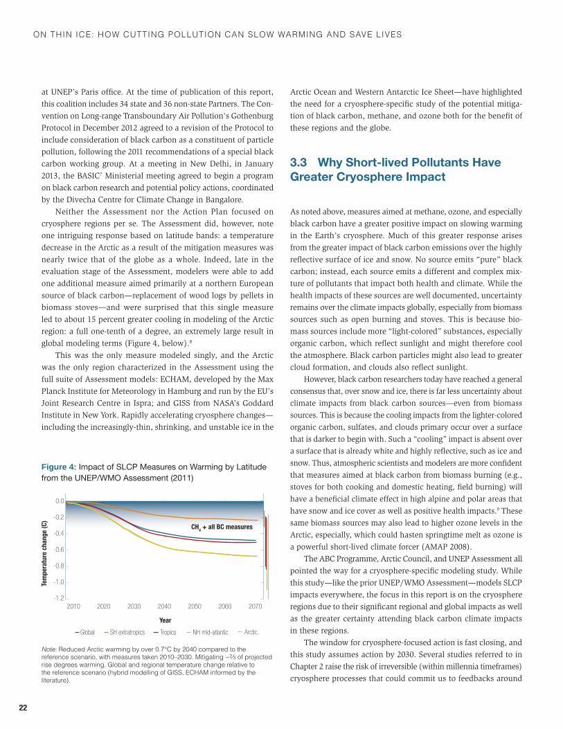
On thin ice: hOw cutting pOllutiOn can slOw warming and save lives
22
at UNEP’s Paris office. At the time of publication of this report, this coalition includes 34 state and 36 non-state Partners. The Con-vention on Long-range Transboundary Air Pollution‘s Gothenburg Protocol in December 2012 agreed to a revision of the Protocol to include consideration of black carbon as a constituent of particle pollution, following the 2011 recommendations of a special black carbon working group. At a meeting in New Delhi, in January 2013, the BASIC7 Ministerial meeting agreed to begin a program on black carbon research and potential policy actions, coordinated by the Divecha Centre for Climate Change in Bangalore.
Neither the Assessment nor the Action Plan focused on cryosphere regions per se. The Assessment did, however, note one intriguing response based on latitude bands: a temperature decrease in the Arctic as a result of the mitigation measures was nearly twice that of the globe as a whole. Indeed, late in the evaluation stage of the Assessment, modelers were able to add one additional measure aimed primarily at a northern European source of black carbon—replacement of wood logs by pellets in biomass stoves—and were surprised that this single measure led to about 15 percent greater cooling in modeling of the Arctic region: a full one-tenth of a degree, an extremely large result in global modeling terms (Figure 4, below).8
This was the only measure modeled singly, and the Arctic was the only region characterized in the Assessment using the full suite of Assessment models: ECHAM, developed by the Max Planck Institute for Meteorology in Hamburg and run by the EU’s Joint Research Centre in Ispra; and GISS from NASA’s Goddard Institute in New York. Rapidly accelerating cryosphere changes—including the increasingly-thin, shrinking, and unstable ice in the
Arctic Ocean and Western Antarctic Ice Sheet—have highlighted the need for a cryosphere-specific study of the potential mitiga-tion of black carbon, methane, and ozone both for the benefit of these regions and the globe.
3.3 Why Short-lived Pollutants Have Greater Cryosphere Impact
As noted above, measures aimed at methane, ozone, and especially black carbon have a greater positive impact on slowing warming in the Earth’s cryosphere. Much of this greater response arises from the greater impact of black carbon emissions over the highly reflective surface of ice and snow. No source emits “pure” black carbon; instead, each source emits a different and complex mix-ture of pollutants that impact both health and climate. While the health impacts of these sources are well documented, uncertainty remains over the climate impacts globally, especially from biomass sources such as open burning and stoves. This is because bio-mass sources include more “light-colored” substances, especially organic carbon, which reflect sunlight and might therefore cool the atmosphere. Black carbon particles might also lead to greater cloud formation, and clouds also reflect sunlight.
However, black carbon researchers today have reached a general consensus that, over snow and ice, there is far less uncertainty about climate impacts from black carbon sources—even from biomass sources. This is because the cooling impacts from the lighter-colored organic carbon, sulfates, and clouds primary occur over a surface that is darker to begin with. Such a “cooling” impact is absent over a surface that is already white and highly reflective, such as ice and snow. Thus, atmospheric scientists and modelers are more confident that measures aimed at black carbon from biomass burning (e.g., stoves for both cooking and domestic heating, field burning) will have a beneficial climate effect in high alpine and polar areas that have snow and ice cover as well as positive health impacts.9 These same biomass sources may also lead to higher ozone levels in the Arctic, especially, which could hasten springtime melt as ozone is a powerful short-lived climate forcer (AMAP 2008).
The ABC Programme, Arctic Council, and UNEP Assessment all pointed the way for a cryosphere-specific modeling study. While this study—like the prior UNEP/WMO Assessment—models SLCP impacts everywhere, the focus in this report is on the cryosphere regions due to their significant regional and global impacts as well as the greater certainty attending black carbon climate impacts in these regions.
The window for cryosphere-focused action is fast closing, and this study assumes action by 2030. Several studies referred to in Chapter 2 raise the risk of irreversible (within millennia timeframes) cryosphere processes that could commit us to feedbacks around
Figure 4: Impact of SLCP Measures on Warming by Latitude from the UNEP/WMO Assessment (2011)
Note: reduced arctic warming by over 0.7°C by 2040 compared to the reference scenario, with measures taken 2010–2030. mitigating ~2⁄3 of projected rise degrees warming. Global and regional temperature change relative to the reference scenario (hybrid modelling of GIss, eCham informed by the literature).
Tem
pera
ture
cha
nge
(C)
-0.6
-0.4
-0.2
0.0
-1.2
-1.0
-0.8
Year
2010 2050204020302020 2060 2070
CH4 + all BC measures
Global SH extratropics Tropics NH mid-atlantic Arctic
the role of short-lIved PollUtants In CryosPhere ProteCtIon
23
sea-level rise, permafrost, or albedo by mid-century within the next few decades if temperature rise in the cryosphere continues unabated. Some cryosphere scientists—alarmed at the rapid and accelerating changes shown by their research—have begun to advocate for geo-engineering in the cryosphere and on larger
scales, with extremely uncertain impacts to regional and global ecosystems.10 It is the hope of this study to provide some insights into more effective, sustainable, developmentally appropriate, and less uncertain mitigation options before it becomes too late for many of these cryosphere regions to be preserved.
Endnotes1 See, for example, Menon et al. (2002). 2 Melting Ice: Regional Dramas, Global Wake-up Call (2009): www.regjeringen.no.3 Arctic Council SLF TF 2011, 20134 Ozone in the context of this report refers to tropospheric or ground level ozone, which contributes to the formation of smog; this is not to be confused with stratospheric ozone. 5 UNEP Policy Brief: Towards an Action Plan for Near-term Climate Protection and Clean Air Benefits.6 Some hydroflourocarbons (HFCs), used in refrigeration, are also short-lived; they are included in CCAC initiatives as short-lived climate pollutants. For near-term cryo-sphere benefits, they do not have the differentiated impact of black carbon and methane over ice and snow, and their atmospheric concentrations today are relatively small. Thus their chief potential lies in avoiding future catastrophic warming by substituting other chemicals for cooling compounds that do not have such negative climate impacts.7 China, India, South Africa, and Brazil.8 All temperature measurements in this study use degrees Celsius (C).9 See especially Bond et al. (2013).10 Physics Today 66:17 (2013). “Scientists Alarmed by Rapidly Shrinking Arctic Ice Cap.”
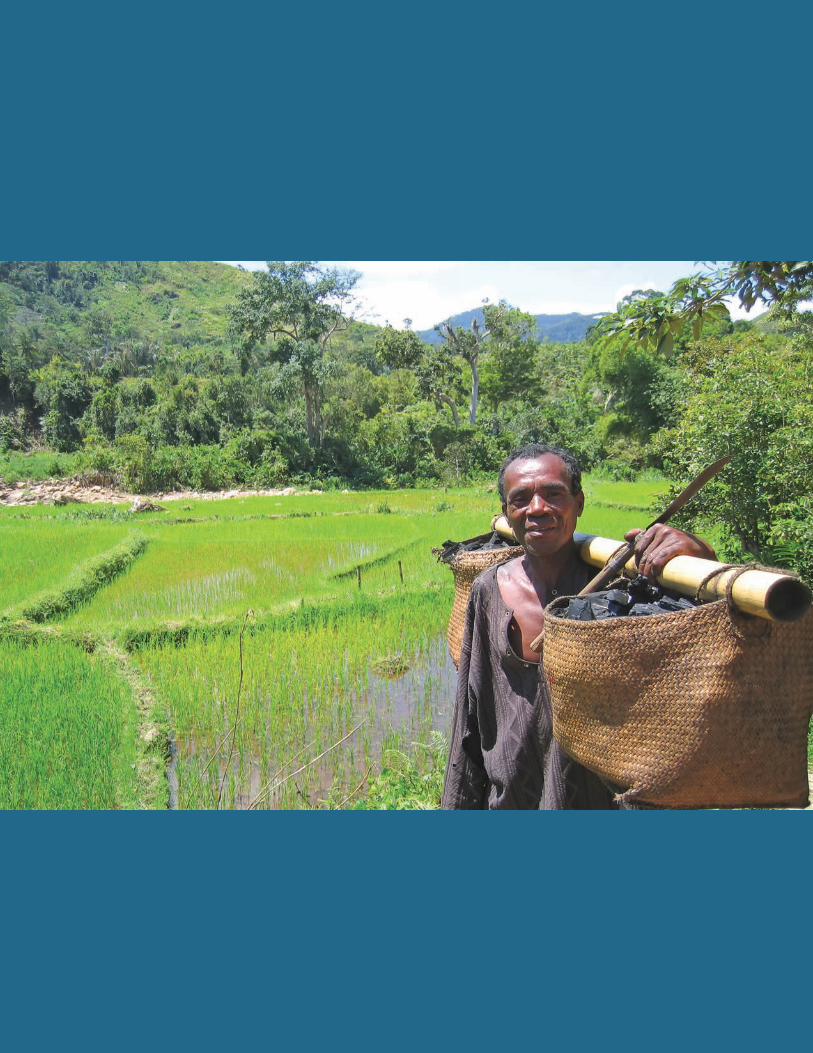
Chapter 4
25
Methods, Measures and Reductions
4.1 Improvements in Models, Emissions Estimates, and Cryosphere Impacts
This chapter briefly outlines the modeled black carbon reduction measures and methods, including improvements in the modeling underlying this report since the UNEP/WMO Assessment. Annex 2 outlines the modeled basis for each measure, modeling param-eters, and assumptions in greater detail.
The UNEP/WMO Assessment identified 16 reduction mea-sures, and broke important new ground in quantifying the over-all potential benefits of short-lived pollutants for health, crops, and climate. These mitigation options were chosen from more than 2,000 possible measures because initial analysis indicated that they: (1) provided both health/crop and near-term climate benefits; and (2) were currently in use around different regions of the world. Other pollution mitigation measures might improve health or bring other important environmental benefits but also speed warming (a classic example is the use of low-sulfur fuels; uses of these fuels improves human health and avoids acid rain but could result in local warming). The Assessment also did not include energy efficiency measures, or technologies that might prove applicable in the future but have not yet been successfully disseminated (such as electric cars or vaccines aimed at decreas-ing methane from enteric fermentation in cattle).
The UNEP Assessment measures were chosen for technical feasibility and their successful implementation somewhere; the Assessment did not, however, evaluate the black carbon and methane measures from a cost-benefit point of view for individual countries or regions. The subsequent UNEP-Science Policy Brief (“Towards an Action Plan for near-term Climate Protection and Clean Air Benefits”) did begin to assess costs. Cost-benefit con-siderations will of course differ from country to country, based on national capacity, health, and/or environment goals. Nevertheless, on a global scale the mitigation measures in the Assessment did prove unique in their ability to slow warming in the near-term
while improving health and/or crop yields through technologies currently in use with potential for scale-up.
Since the Assessment, updates and/or improvements have occurred in the underlying emissions data, in estimates of how the measures might impact emissions, and in the way the mod-els show the impact of reductions. This is especially the case for stoves, both heating and cooking; for open burning; and for oil and gas flaring. The understanding of the amount of forcing by black carbon has also improved, per the discussion in Chapter 3, especially over cryosphere regions. These improvements are reflected in data used for this report.
Although it also assesses methane measures, this report’s modeling focused primarily on demonstrating the benefits of black carbon measures because of their importance to both local health and to potentially slowing warming in nearby cryosphere regions. It involved three separate modeling teams, two of which also participated in the UNEP/WMO Assessment. The teams used a total of four different global atmospheric models deployed for a variety of forecasting purposes, from air pollution to the reports of the Intergovernmental Panel on Climate Change (including AR5). More than 40 experts in climate modeling, health benefits, and agriculture were invited to review the methodologies sum-marized in Annex II. Many of the 100+ UNEP/WMO Assess-ment reviewers, supplemented by over three dozen additional new cryosphere researchers and policymakers, were also invited to assess the results and provide comments. In addition to the modeling teams, ICCI, and World Bank teams, nearly 60 scien-tists, experts and policymakers provided comments or otherwise contributed to the report.
The modeling teams for the first time considered the impacts of black carbon measures individually. This yielded global map-ping that indicates which black carbon measure(s) have the greatest impact on which cryosphere region(s). These results were then run through three sets of assumptions about black and organic carbon’s radiative forcing, an issue which remains in some dispute due to different estimates as to their effects on
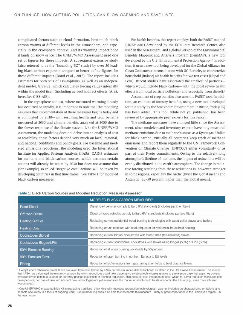
On thin ice: hOw cutting pOllutiOn can slOw warming and save lives
26
complicated factors such as cloud formation, how much black carbon warms at different levels in the atmosphere, and espe-cially in the cryosphere context, and its warming impact once it lands on snow or ice. The UNEP/WMO Assessment used one set of figures for these impacts. A subsequent extensive study (also referred to as the “bounding BC” study) by over 30 lead-ing black carbon experts attempted to better define figures for these different impacts (Bond et al., 2013). The report includes estimates for both sets of assumptions, as well as an indepen-dent model, GISS-E2, which calculates forcing values internally within the model itself (including aerosol indirect effects (AIE); hereafter GISS AIE).
In the cryosphere context, where measured warming already has occurred so rapidly, it is important to note that the modeling assumes that implementation of these measures begins today and is completed by 2030—with resulting health and crop benefits measured at 2030 and climate benefits analyzed at 2050 due to the slower response of the climate system. Like the UNEP/WMO Assessment, the modeling does not delve into an analysis of cost or feasibility; these factors depend very much on local, regional, and national conditions and policy goals. For baseline and mod-eled emissions reductions, the modeling used the International Institute for Applied Systems Analysis (IIASA) GAINS estimates for methane and black carbon sources, which assumes certain actions will already be taken by 2030 but does not assume that (for example) so-called “negative cost” actions will be taken by developing countries in that time frame.1 See Table 1 for modeled black carbon measures.
For health benefits, this report employs both the FASST method (UNEP 2011) developed by the EC’s Joint Research Center, also used in the Assessment, and a global version of the Environmental Benefits Mapping and Analysis Program (BenMAP), a new tool developed by the U.S. Environmental Protection Agency.2 In addi-tion, it uses a new tool being developed for the Global Alliance for Clean Cookstoves in consultation with UC-Berkeley to characterize household (indoor) air health benefits for two test cases (Nepal and Peru). Recent studies have associated the smallest of particles—which would include black carbon—with the most severe health effects from local particle pollution (and especially from diesel).3
Assessment of crop benefits also uses the FASST tool. In addi-tion, an estimate of forestry benefits, using a new tool developed for this study by the Stockholm Environment Institute, York (UK) has been added. This tool, while not yet published, has been reviewed by appropriate peer experts for this report.
The methane measures have changed little since the Assess-ment, since modelers and inventory experts have long measured methane emissions due to methane’s status as a Kyoto gas. Unlike for black carbon, virtually all countries keep track of methane emissions and report them regularly to the UN Framework Con-vention on Climate Change (UNFCCC) either voluntarily or as part of their Kyoto commitments. Owing to the relatively long atmospheric lifetime of methane, the impact of reductions will be evenly distributed in the earth’s atmosphere. The change in radia-tive forcing resulting from these reductions is, however, stronger in some regions, especially the Arctic (twice the global mean) and Antarctic (20–50 percent higher than the global mean).
a Except where otherwise noted, these are taken from calculations by IIASA on “maximum feasible reductions” as stated in the UNEP/WMO assessment This means that IIASA has calculated the maximum amount by which reductions could take place using existing technologies relative to a reference case that assumes current emission levels continue, except for currently passed legislation or planned regulation. This does not take into account cost, which for some reduction measures can be expensive; nor does it take into account new technologies not yet available on the market or which could be developed in the future (e.g., even more efficient woodstoves). b One UNEP/WMO measure, Brick Kilns (replacing traditional brick kilns with improved production technologies), was not included as characterizing emissions and impacts accurately is a focus of ongoing work. future modeling should be able to incorporate this measure – likely of great importance in the himalayan region – in the near future.
Table 1: Black Carbon Sources and Modeled Reduction Measures Assesseda
MODELED BLACK CARBON MEASURESb
Road Diesel Diesel road vehicles comply to Euro 6/VI standards (includes particle filters)
Off-roadDiesel Diesel off-road vehicles comply to Euro 6/VI standards (includes particle filters)
Heating Biofuel replacing current residential wood-burning technologies with wood pellet stoves and boilers
Heating Coal replacing chunk coal fuel with coal briquettes for residential household heating
Cookstoves Biofuel Replacing current biofuel cookstoves with forced draft (fan-assisted) stoves
Cookstoves Biogas/LPG Replacing current solid biofuel cookstoves with stoves using biogas (50%) or LPG (50%)
50% Biomass Burning reduction of all open burning worldwide by 50 percent
90% Eurasian Fires reduction of open burning in northern eurasia to eU levels
Flaring Reduction of BC emissions from gas flaring at oil fields to best practice levels
methods, measUres and redUCtIons
27
4.2 Stoves
These measures include stoves using biomass fuel (primarily wood, but also agricultural residue and dung cake in some regions) used for cooking or heating (occasionally, combined cooking and heating). Emissions from biomass-based stoves have been asso-ciated with higher levels of some cancers, respiratory illnesses, and deaths, especially among children under age five and women cooking over open flames inside the home.
Modeled Stove Measures
Cooking Stoves
Two distinct measures were modeled for cooking stoves:
Replacement of current biomass stoves for cooking by stoves that incorporate fans, which improves combustion.
Replacement of current biomass stoves for cooking by a 50–50 mix of stoves using LPG and stoves using biogas.
These measures were modeled in separate runs. In reality, replacement with LPG and biogas may not be possible in many rural communities. These runs are an improvement over the UNEP/WMO Assessment modeling, with more precise emissions inventories and BC/OC coefficients from stoves. The Assessment climate modeling only looked at removing all black carbon from stoves rather than testing two specific reduction methods; this effort allows a comparison between the two in health and climate terms.
Heating Stoves
Biomass Heating Stoves: Replacement of current wood stoves and residential boilers used for heating by pellet stoves and boilers.
This measure primarily applies in North American and Europe (primarily the northern tier of countries), where there have been recent increases in the use of wood for heating. The measure also for the first time includes seasonal inventories, better reflecting actual use patterns where wood burning for heating occurs during the colder part of the year.
Coal Heating/Cooking Stoves
Replacement of chunk coal fuel with coal briquettes.
This measure applies to some countries in Eastern Europe, where coal remains a plentiful fuel source at the household level;
to China; and to some Himalayan communities. As with biomass heating stoves, this measure now includes more realistic seasonal use patterns. Many coal stoves provide at least some cooking potential as well.
4.3 Diesel
Diesel land transport (automobiles and trucks); off-road diesel vehicles, such as construction or farming equipment, snowmobiles, etc. Diesel generator use is a growing and potentially important source, but the emissions estimates do not yet exist that would have allowed their inclusion in this study. Emissions from diesel are very high in percentage of black carbon, second only to kerosene lanterns, and have been associated with a number of health issues (primarily respiratory and cardiac, but also cancers).
Modeled Diesel Measures
On-road diesel vehicle and associated fuel improvements.
Off-road diesel vehicle and associated fuel improvements, including equipment used in construction, farming, and the like.
This measure involves replacement of land and off-road vehicles either by new lower emitting vehicles (EURO VI standards) or by retrofitting vehicles with particle filters.4
4.4 Open Burning
New to this study, all fires as observed by MODIS satellite (which detects fires as small as 50 m2 in size) were mapped. This primar-ily includes set fires for agricultural or forestry purposes; pasture fires; and forest and grass fires caused by accident from human activity, including those spreading unintentionally from set fires (very few fires globally begin with lightening strikes outside of the high Arctic boreal or some high altitude forests) (Peterson et al 2010).
It is important to note that estimated emissions from such burn-ing include a larger number of substances than from most other sources—not just black carbon, but also other warming agents, (e.g., carbon monoxide (CO) and methane) and cooling agents such as sulfates and organic carbon. As with stoves, this combination, including the lighter substances (such as organic carbon), still leads to higher radiative forcing over cryosphere regions. The sheer size of fire emissions makes them a major black carbon source in climate terms; it also causes significant infrastructure damage and health problems. In addition to 50 deaths and over 2000 damaged buildings caused directly by the 2010 fires in Russia, for example,
On thin ice: hOw cutting pOllutiOn can slOw warming and save lives
28
the Russian Economic Development Ministry reported that over 55,000 additional deaths occurred there (compared to 2009) from the combination of fire pollution and extreme heat during July and August (IFFN-GFMC 2011).
At this time, fire emissions estimates do not include peat fires, which can emit large amounts of methane or CO2, as these are generally not detectable by satellite and can burn underground for an entire summer season.
Modeled Open Burning Measures
A 50-percent reduction in open burning globally.
A 90-percent reduction in open burning in northern Eurasia.
For the purposes of this report, the main reduction measure assumes a decrease of 50 percent in all regions, as measured by satellite data. This 50-percent figure likely represents an overes-timate of potential control of fires in high boreal areas, which are sparsely populated and where estimates range from 30–50 percent for lightning or spontaneous combustion fires; and an underestimate of maximum feasible reductions in other regions, where the percentage of lightning-caused fires is estimated at well under 5 percent (i.e., a highly conservative estimate). This is reflected in the second modeled open measure, which assumes a 90-percent decrease in fires in northern Eurasia. This figure is based on a satellite comparison of this region (defined as 45–60 degrees North and 30–140 degrees East) to regions in similar Western European land areas where burning is strictly regulated; the satellite comparison was conducted for this study and shows a 90-percent decrease in fires in the region.
4.5 Flaring from Oil and Gas
Locations of flares are determined by DMSP and MODIS satellite data, with volumes of flared gas characterized by the World Bank’s Global Gas Flaring Reduction Initiative. It should be noted that this study does not include a potentially significant new source of flaring which may be occurring in connection with shale gas extraction in North America, which is increasingly being detected by nighttime satellite data (VIRRS).
Modeled Flaring Measure
Introduction of flaring best practices per Norwegian and Danish regulations.
Some flaring by the oil and gas industry is inevitable, but these standards cut flaring to only those circumstances that require it and ensure more complete combustion. This study improves the
measure through better spatial resolution of the exact location and magnitude of flares, building strongly on the work of the EU-supported ECLIPSE Project.
4.6 Note on Black Carbon Measures Not Included
The UNEP/WMO Assessment showed little overall global impact from brick kilns, probably because current emissions estimates are lower than reality and/or do not adequately reflect location. Brick kilns may prove especially important in relation to the Himalayas, where local kilns may have large health and climate impacts. Indeed, an estimated 100,000 kilns in the Indo-Gangetic Plains are potentially upwind of the Himalayan cryosphere, so kilns should be incorporated in future studies there.5 As noted above, diesel generators are also a source that may prove important but that need improved data on emissions patterns.
The UNEP/WMO Assessment did not include coal-fired power plants because their emissions of sulfates cool the atmosphere, and few particles (including black carbon) are emitted with cur-rent emission control technology on plant smokestacks. However, particle emissions, especially from older plants lacking emission control technologies, can lead to difficult air pollution problems in some regions. The particles emitted from such plants may have a significant forcing effect near glaciers and snowpack, even with sulfur emissions taken into account; this potential impact remains to be studied.
In addition, the modeling did not include shipping or air trans-port. As a result of the efficiency of jet engines, they produce little black carbon—though they can have extremely localized effects on stratospheric ozone and cloud formation. ICAO has kept this issue under review, considering aircraft design, fuels, combustion efficiency, and flight operations.
The release of greenhouse gases and air pollutants from international shipping has a complex effect on the climate: greenhouse gas emissions have a warming effect while some co-emitted air pollutants actually lead to cooling. In some areas, ships can contribute up to 20–30 percent of the local fine particu-late matter (PM 2.5), and up to 15 percent of ground-level ozone concentrations (European Environment Agency 2013). Shipping represents less than three percent of total anthropogenic black carbon emissions globally and also produces significant levels of ozone precursors; modeling at this stage, however, is unable to capture the impacts. Studies on Svalbard in the Arctic have indicated that local emissions from shipping may be the largest source of deposited black carbon in the Svalbard archipelago, and it likely represents one of the larger sources for Antarctica as well. As sea ice melts and commercial activities increase,
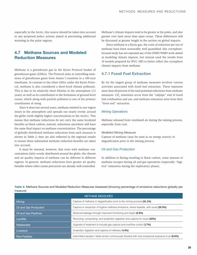
methods, measUres and redUCtIons
29
especially in the Arctic, this source should be taken into account in any proposed policy actions aimed at preventing additional warming in the polar regions.
4.7 Methane Sources and Modeled Reduction Measures
Methane is a greenhouse gas in the Kyoto Protocol basket of greenhouse gases (GHGs). The Protocol aims at controlling emis-sions of greenhouse gases from Annex I countries in a 100-year timeframe. In contrast to the other GHGs under the Kyoto Proto-col, methane is also considered a short-lived climate pollutant. This is due to its relatively short lifetime in the atmosphere (12 years) as well as its contribution to the formation of ground-level ozone, which along with particle pollution is one of the primary constituents of smog.
Since it does last several years, methane emitted in one region mixes in the atmosphere and spreads out nearly evenly around the globe (with slightly higher concentrations in the Arctic). This means that methane reductions do not carry the same localized benefits as black carbon; instead, reductions anywhere will have the same final impact on methane concentrations. The percentage of globally distributed methane reductions from each measure is shown in Table 2; they are also reflected in the regional results to ensure these substantial methane reduction benefits are taken into account.
It must be stressed, however, that even with methane con-centrations fairly evenly distributed around the globe, the climate and air quality impacts of methane can be different in different regions. In general, methane reductions have greater air quality benefits where other ozone precursors are already well-controlled.
Methane’s climate impacts tend to be greater at the poles, and also greater over land areas than open ocean. These differences will be discussed at greater length in the section on global impacts.
Since methane is a Kyoto gas, the costs of reduction per ton of methane have been reasonably well quantified; this cryosphere-focused study has not repeated any of the UNEP/WMO work aimed at modeling climate impacts, but instead used the results from 10 models prepared for IPCC AR5 to better reflect the cryosphere climate impacts from methane.
4.7.1 Fossil Fuel Extraction
By far the largest group of methane measures involves various activities associated with fossil fuel extraction. These represent more than 60 percent of the total potential reductions from methane measures. CO2 emissions occur from the “tailpipe” end of fossil fuel combustion and use, and methane emissions arise from their “front end” extraction.
Mining Operations
Methane released from ventilated air during the mining process, especially from coal.
Modeled Mining MeasureCapture of methane (may be used as an energy source) or degasification prior to the mining process.
Oil and Gas Production
In addition to flaring resulting in black carbon, some amount of methane escapes during oil and gas operations (especially “fugi-tive” emissions during the exploratory phase).
Table 2: Methane Sources and Modeled Reduction Measures Assessed (showing percentage of emissions reductions globally per measure)
METHANE MEASURES
Mining Capture of methane or degasification prior to the mining process (31.1%)
Oil and Gas Production Capture or reinjection of fugitive methane emissions, where feasible, with reuse (30.3%)
Oil and Gas Pipelines reduced leakage through improved monitoring and repair (4.9%)
Landfills recycling, composting, and anaerobic digestion and capture for reuse (20%)
Wastewater Upgrade of treatment to include gas capture and overflow control (2.7%)
Livestock anaerobic digestion and capture of methane (4.4%)
Rice Paddies Intermittent aeration: fields remain continuously flooded with only occasional exposure to air (6.6%)
On thin ice: hOw cutting pOllutiOn can slOw warming and save lives
30
Modeled Oil and Gas Measures
Capture or reinjection of fugitive methane emissions, where feasible, with reuse.
For pipelines, reduced leakage through improved monitoring and repair.
Note that flaring of emissions is not considered a viable reduc-tion measure for near-term health or climate benefits, as this can produce black carbon and other particle pollution unless flaring is done extremely efficiently. Reuse, on the other hand, can result in a decrease in black carbon emissions, with numerous health and development benefits (e.g., when the captured gas is used for LPG/biogas cookstoves or to replace diesel with gas engine gen-erators). This added co-benefit is not yet captured in the modeled measure; the potential exists, however, for far greater secondary use of fugitive emissions than exists today.
It should also be noted that the GAINS estimates used do not yet include fugitive methane emissions from either the newer fracturing-and-extraction method or from shale gas. Both methods can result in large methane leakage. As with more conventional oil and gas extraction methods, there exist industry standards that can minimize such leakage to a very large degree; a voluntary consortium has been formed in the United States to promote these methods (Center for Sustainable Shale Development CSSD).
Leakage from long-distance transport pipelines occurs to an especially large extent in northern latitudes where shifting per-mafrost leads to breakage and where monitoring presents a chal-lenge due to the extreme environment. Such measures can prove extremely cost-effective for producers, and have provided one of the more successful project areas under the Clean Development Mechanism (CDM).
4.7.2 Waste
Landfills
Modeled Landfill Measure
Recycling, composting, and anaerobic digestion and capture for reuse.
As garbage decays in landfills, it releases large amounts of methane gas, which can leak from under the ground even decades after burial. Note that under the model this also includes flar-ing of the gas, which might lead to release of black carbon and
should therefore not be considered an acceptable alternative to reduce black carbon emissions. Recapture and use of gas as biogas for fuel, including for automobiles, may occur as part of the collection process; existing landfills may also be retrofitted with gas collectors.
Wastewater Handling and treatment of sewage and stormwater runoff.
Modeled Wastewater Measure
Upgrade of wastewater treatment to include gas capture and overflow control.
This measure involves improved handling and treatment of sewage and stormwater runoff; in many cases in developing coun-tries, this involves the total introduction of such systems where they do not exist. Note that health estimates for this measure do not include improvements from better control of waterborne diseases, a large cause of illness around the world (second in the current Global Burdens of Disease list).
4.7.3 Agriculture
Agriculture represents one of the largest sources of methane globally, including some from open burning and especially when wildfires spread to peat as noted above. The largest sources of agricultural methane emissions however include livestock and wet agricultural methods, especially rice cultivation.
Livestock
Methane emissions arise from manure, primarily from cattle and pigs, as well as enteric fermentation from cattle.
Modeled Livestock Measure
Anaerobic digestion and capture of methane Livestock is a large and growing source of methane globally as
demand for meat-based diets rises. The only practical measure at this time involves anaerobic digestion and capture of methane for fuel on large-scale cattle and pig farms. Relatively new commercial technologies, especially in Sub-Saharan Africa, have adapted this technology for small farm and household use, with direct conver-sion of the methane capture to biogas used for cooking—and even conversion to small-scale electricity generation (e.g., for charging of cell phones).

methods, measUres and redUCtIons
31
Rice Paddies
Methane is generated from wet cultivation of rice due to flooding and the subsequent draining of the rice fields; the decaying crop residue remaining after the fields are drained emits methane.
Modeled Rice Paddy Measure
Intermittent aeration: Fields remain continuously flooded with only occasional exposure to air.
Endnotes1 Greenhouse Gas – Air Pollution Interactions and Synergies (GAINS). See http://gains.iiasa.ac.at/models/.2 The tool is accessible at http://www.epa.gov/air/benmap/.3 International Agency for Research on Cancer (2012). 4 This measure was assessed as a ”high cost” measure relative to some of the others in the UNEP Action Plan (2012), and consideration of cost and feasibility should be assessed in a country-specific context.5 Shakti Sustainable Energy Foundation (2012).
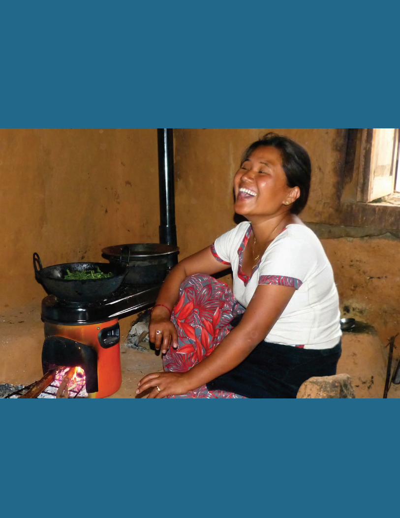
Chapter 5
33
CryosphereBenefits: Where Health and Climate Intersect
The following section summarizes the modeling results for each cryosphere region. It also looks at global, “pan-cryosphere” impacts such as sea level-rise, as well as health
and crop benefits.As noted earlier, proximity matters when it comes to the cli-
mate impact of black carbon. Sources of black carbon emissions have their greatest impact on nearby cryosphere regions because most black carbon falls out of the atmosphere relatively quickly. The health impacts from black carbon and other particle pollution from these same sources are even more local—and strongest clos-est to the source. The health impacts from transport sources such as diesel, for example, are higher along highly-trafficked streets compared to routes just a few blocks away. For this reason, the health benefits of BC source reductions have been defined for what this study terms the primary BC source areas for each of the five major cryosphere regions studied (Table 3).
For the Arctic, the primary BC source regions include Arctic Council nations plus some countries in northern Europe. For the Himalayas, Andes, and East African Highlands, source regions include countries that contain some portion of these highlands or mountains. In the case of Antarctica, which is distant from any black carbon source, health results are assessed for the extreme southern tier of nearby continents; here, however, the “source region” relationship is far weaker than for any other cryosphere region. There is some observational evidence that these areas
may contribute greater relative black carbon impacts, especially on the Antarctic Peninsula (e.g., from tracking of smoke clouds from wildfires in Australia or Patagonia).
For health, outcomes are expressed in terms of avoided deaths in the source regions, using the BenMAP tool1 which calculates health benefits of avoided emissions relative to baseline health data from the 2010 Global Burden of Disease (GBD) (Lim et al. 2012). The GBD identifies solid-fuel use as a major cause of mortality due to the ambient outdoor pollution they create and the indoor exposure to families while cooking or spending time inside their homes. Currently available models only include impacts of air pollution that reach the outdoor environment. Multiple studies indicate, however, that the number of deaths due to exposure to smoke inside and immediately around the home (termed household exposure) from sources such as cookstoves may be far greater.
The Global Burden of Disease has estimated 4 million deaths per year from cookstoves: 3.5 million from household exposure and an additional 500,000 due to cookstoves’ contributions to ambient outdoor pollution. This is a 7:1 ratio on the global scale. The regional discussions below note where additional deaths from household exposure would be expected alongside the report’s modeled results for outdoor pollution.
For climate, results are summarized in terms of a decrease in radiative forcing in each region, using the regions shown in
Table 3: Primary Cryosphere Black Carbon Source Regions
Andes Argentina, Bolivia, Brazil, Ecuador, Peru, Venezuela, Chile
Arctic Belarus, Belgium, Canada, denmark, estonia, finland, france, Germany, Ireland, latvia, lithuania, netherlands, norway, Poland, russia, sweden, Ukraine, United Kingdom, United states of america
Antarctic argentina, australia, Chile, new Zealand, south africa
East Africa Congo (Democratic Republic), Eritrea, Ethiopia, Kenya, Uganda, Tanzania
Himalayas Afghanistan, Bangladesh, Bhutan, Cambodia, China, India, Kazakhstan, Kyrgyz Republic, Laos, Mongolia, Myanmar, Nepal, Pakistan, Tajikistan, Uzbekistan
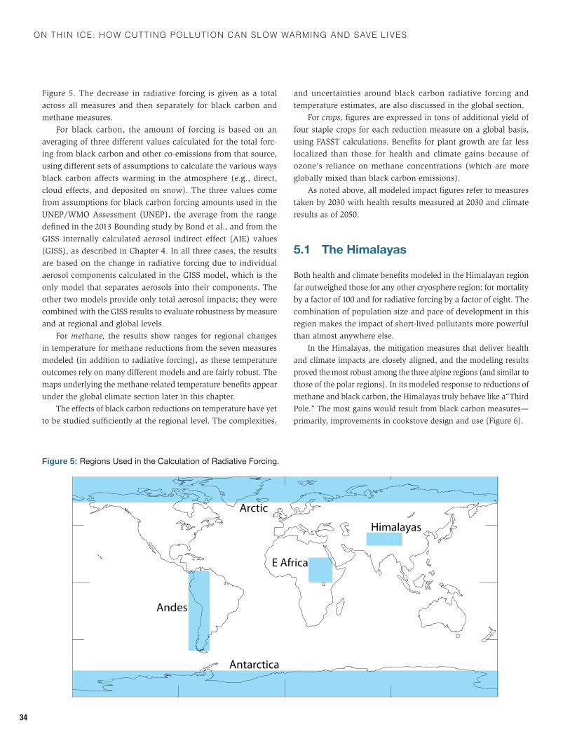
On thin ice: hOw cutting pOllutiOn can slOw warming and save lives
34
Figure 5. The decrease in radiative forcing is given as a total across all measures and then separately for black carbon and methane measures.
For black carbon, the amount of forcing is based on an averaging of three different values calculated for the total forc-ing from black carbon and other co-emissions from that source, using different sets of assumptions to calculate the various ways black carbon affects warming in the atmosphere (e.g., direct, cloud effects, and deposited on snow). The three values come from assumptions for black carbon forcing amounts used in the UNEP/WMO Assessment (UNEP), the average from the range defined in the 2013 Bounding study by Bond et al., and from the GISS internally calculated aerosol indirect effect (AIE) values (GISS), as described in Chapter 4. In all three cases, the results are based on the change in radiative forcing due to individual aerosol components calculated in the GISS model, which is the only model that separates aerosols into their components. The other two models provide only total aerosol impacts; they were combined with the GISS results to evaluate robustness by measure and at regional and global levels.
For methane, the results show ranges for regional changes in temperature for methane reductions from the seven measures modeled (in addition to radiative forcing), as these temperature outcomes rely on many different models and are fairly robust. The maps underlying the methane-related temperature benefits appear under the global climate section later in this chapter.
The effects of black carbon reductions on temperature have yet to be studied sufficiently at the regional level. The complexities,
and uncertainties around black carbon radiative forcing and temperature estimates, are also discussed in the global section.
For crops, figures are expressed in tons of additional yield of four staple crops for each reduction measure on a global basis, using FASST calculations. Benefits for plant growth are far less localized than those for health and climate gains because of ozone’s reliance on methane concentrations (which are more globally mixed than black carbon emissions).
As noted above, all modeled impact figures refer to measures taken by 2030 with health results measured at 2030 and climate results as of 2050.
5.1 The Himalayas
Both health and climate benefits modeled in the Himalayan region far outweighed those for any other cryosphere region: for mortality by a factor of 100 and for radiative forcing by a factor of eight. The combination of population size and pace of development in this region makes the impact of short-lived pollutants more powerful than almost anywhere else.
In the Himalayas, the mitigation measures that deliver health and climate impacts are closely aligned, and the modeling results proved the most robust among the three alpine regions (and similar to those of the polar regions). In its modeled response to reductions of methane and black carbon, the Himalayas truly behave like a“Third Pole.” The most gains would result from black carbon measures—primarily, improvements in cookstove design and use (Figure 6).
Figure 5: Regions Used in the Calculation of Radiative Forcing.
Andes
E Africa
Himalayas
Antarctica
Arctic
CryosPhere BenefIts: where health and ClImate InterseCt
35
Cryosphere and Regional Climate Benefits
There are challenges to modeling temperature impacts from black carbon, and forcing in adjacent regions also influences the climate over the Himalayas. Yet the decrease in radiative forcing resulting
from black carbon measures in the Himalayas is large enough to yield regional climate benefits with almost equal certainty as those occurring in the polar regions. As with other land areas, methane reductions have a greater impact in the Himalayas than the global mean in terms of temperature, with an annual avoided rise of about 0.3 degrees by 2050. This could significantly slow glacial melt, as well as perturbations to regional water resources arising from glacier and snowpack melt, by moving the freeze line downward in altitude.
Reductions of methane and black carbon could help stabilize water resources in some of the Himalayan watersheds, assuming the measures lead to a slowing of the glacier retreat observed in many of these watersheds. These effects could be most visible in the Indus and Tarim river systems, which are the most depen-dent on melt runoff. The arid Tarim river system relies almost exclusively on Himalayan runoff from glacier, snow melt, and precipitation. Researchers working in the Tarim have observed perturbations to these patterns especially since 1986, and attribute at least some of these changes to increased ice melt and also to greater evaporation from higher ambient temperatures (Zhang et al. 2009; Xu et al. 2006).
In this and other systems, the impacts would be felt at the opposite extreme as well—that is, when melting reaches its peak—in terms of potential flooding and glacial lake flood outburst events. Predicting more precisely the direction and duration of these differ-ent cycles of flood (with added melt) and seasonal drought (as ice and snow cover diminishes) remains an issue for active and more regionally based research. Given the large potential decrease in radiative forcing, however, there is excellent potential to mitigate and slow such changes in the near term.
The impact of black carbon measures on precipitation is even harder to characterize, at least in terms of cryosphere effects. In the case of South Asia, however, the pollution itself has had a demonstrated impact on, and caused perturbation of, the Indian monsoon, according to the work under UNEP’s Atmospheric Brown Cloud (ABC) initiative.
There is a great deal of variability between the models and studies used in this report, as well as in UNEP’s Atmospheric Brown Cloud studies, regarding the effects of pollutants and pollutant mitigation on rainfall patterns. All the models show, however, increased changes in the monsoon based on atmospheric pollution levels. These changes threaten farming practices and the reliability of water supplies for household use, and might also create higher risks of flooding from more extreme monsoon events, as occurred in June 2013 in northern India. Decreasing pollution from these sources should help moderate such changes and provide additional time for both adaptation of farming and household practices and disaster preparedness. Pursuing both paths will provide local populations with the greatest chance of building resilience to repeated weather-related disasters.
Box 1: Modeled Benefits in the Himalayas
this broad swath of central and south asia includes many devel-oping nations where cookstoves, agricultural and open burning, and polluting diesel engines present development challenges. Implementation of the black carbon mitigation measures as-sessed in this report yield the greatest benefits in the Himalayas relative to any other region considered.
Cryosphere/Climate* Benefits:
• total decrease in radiative forcing, all measures: –7.6 w/m2 (–3.3 to –11.9)
• decrease from black carbon measures: –7.3 w/m2 (–3.0 to –11.6)
• decrease from methane measures: –0.32 w/m2
• annual avoided temperature increase from methane mea-sures: about 0.3°C
(Note global average anthropogenic radiative forcing is approxi-mately 2.3 W/m2)
Health** and Agricultural Benefits in Himalayas Source Region:
• annual premature mortality avoided: 1,238,000• annual increase in staple crops: 15.4 million metric tons
Greatest black carbon benefits: cookstoves (about 75 percent of impacts), road diesel and off-road mobile diesel, open burning
Greatest methane benefits: oil and gas, coal mines, landfills (85 percent of impacts).
* Climate benefits are presented in units of decreased radiative forcing averaged over the region of interest. for comparison, globally averaged anthropogenic forcing from ar5 is 2.3 w/m2; while this regional average does not compare directly with a global average, it is noted to provide a sense of scale compared to the total warming across the globe. ** The public health benefits listed here refer only to the premature mortality avoided due to reductions in ambient (outdoor) air pollution. Some of the measures (principally cookstoves) would also have a significant impact on household (indoor and immediately surrounding the home). This avoided household/indoor exposure is not included in the health benefits estimated above. Text Box 2 explores how improved tools would enable estimates of additional benefits due to the impact of reductions on household air quality.
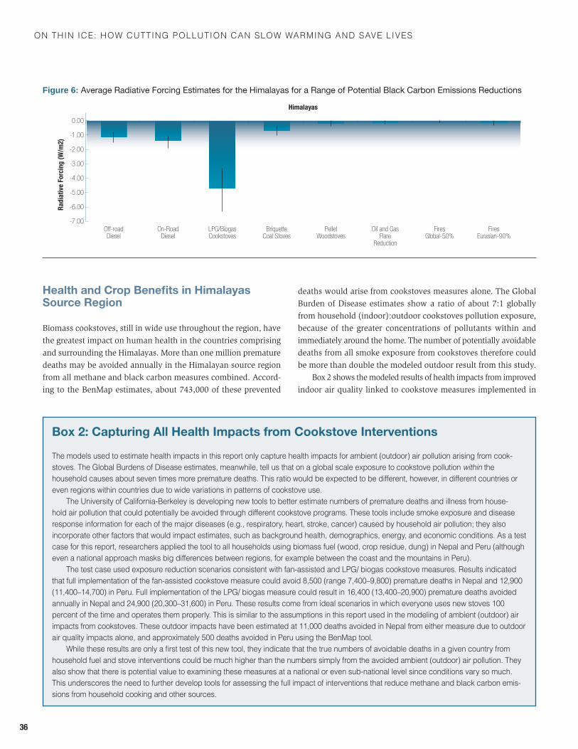
On thin ice: hOw cutting pOllutiOn can slOw warming and save lives
36
Health and Crop Benefits in Himalayas Source Region
Biomass cookstoves, still in wide use throughout the region, have the greatest impact on human health in the countries comprising and surrounding the Himalayas. More than one million premature deaths may be avoided annually in the Himalayan source region from all methane and black carbon measures combined. Accord-ing to the BenMap estimates, about 743,000 of these prevented
deaths would arise from cookstoves measures alone. The Global Burden of Disease estimates show a ratio of about 7:1 globally from household (indoor):outdoor cookstoves pollution exposure, because of the greater concentrations of pollutants within and immediately around the home. The number of potentially avoidable deaths from all smoke exposure from cookstoves therefore could be more than double the modeled outdoor result from this study.
Box 2 shows the modeled results of health impacts from improved indoor air quality linked to cookstove measures implemented in
Figure 6: Average Radiative Forcing Estimates for the Himalayas for a Range of Potential Black Carbon Emissions Reductions
Radi
ativ
e Fo
rcin
g (W
/m2)
-3.00
-2.00
-1.00
0.00
-6.00
-5.00
-4.00
Himalayas
-7.00Off-roadDiesel
On-RoadDiesel
LPG/BiogasCookstoves
BriquetteCoal Stoves
PelletWoodstoves
Oil and GasFlare
Reduction
FiresGlobal-50%
FiresEurasian-90%
Box 2: Capturing All Health Impacts from Cookstove Interventions
The models used to estimate health impacts in this report only capture health impacts for ambient (outdoor) air pollution arising from cook-stoves. The Global Burdens of Disease estimates, meanwhile, tell us that on a global scale exposure to cookstove pollution within the household causes about seven times more premature deaths. This ratio would be expected to be different, however, in different countries or even regions within countries due to wide variations in patterns of cookstove use.
the University of California-Berkeley is developing new tools to better estimate numbers of premature deaths and illness from house-hold air pollution that could potentially be avoided through different cookstove programs. These tools include smoke exposure and disease response information for each of the major diseases (e.g., respiratory, heart, stroke, cancer) caused by household air pollution; they also incorporate other factors that would impact estimates, such as background health, demographics, energy, and economic conditions. as a test case for this report, researchers applied the tool to all households using biomass fuel (wood, crop residue, dung) in Nepal and Peru (although even a national approach masks big differences between regions, for example between the coast and the mountains in Peru).
The test case used exposure reduction scenarios consistent with fan-assisted and LPG/ biogas cookstove measures. Results indicated that full implementation of the fan-assisted cookstove measure could avoid 8,500 (range 7,400–9,800) premature deaths in Nepal and 12,900 (11,400–14,700) in Peru. Full implementation of the LPG/ biogas measure could result in 16,400 (13,400–20,900) premature deaths avoided annually in Nepal and 24,900 (20,300–31,600) in Peru. These results come from ideal scenarios in which everyone uses new stoves 100 percent of the time and operates them properly. This is similar to the assumptions in this report used in the modeling of ambient (outdoor) air impacts from cookstoves. these outdoor impacts have been estimated at 11,000 deaths avoided in nepal from either measure due to outdoor air quality impacts alone, and approximately 500 deaths avoided in Peru using the BenMap tool.
While these results are only a first test of this new tool, they indicate that the true numbers of avoidable deaths in a given country from household fuel and stove interventions could be much higher than the numbers simply from the avoided ambient (outdoor) air pollution. They also show that there is potential value to examining these measures at a national or even sub-national level since conditions vary so much. this underscores the need to further develop tools for assessing the full impact of interventions that reduce methane and black carbon emis-sions from household cooking and other sources.
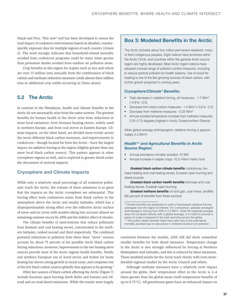
CryosPhere BenefIts: where health and ClImate InterseCt
37
Nepal and Peru. This new2 tool has been developed to assess the total impact of cookstove interventions based on detailed, country-specific exposure data for multiple regions of each country (Annex 2). The work strongly indicates that household-related mortality avoided from cookstoves programs could be many times greater than premature deaths avoided from outdoor air pollution alone.
Crop benefits in this region for staples such as rice and wheat are over 15 million tons annually from the combination of black carbon and methane reduction measures (with almost three million tons in additional crop yields occurring in China alone).
5.2 The Arctic
In contrast to the Himalayas, health and climate benefits in the Arctic do not necessarily arise from the same sources. The greatest benefits for human health in the Arctic arise from reductions in more local emissions: from biomass heating stoves, widely used in northern Europe, and from coal stoves in Eastern Europe. Cli-mate impacts, on the other hand, are divided more evenly across the seven different black carbon measures, and improvements to cookstoves—though located far from the Arctic—have the largest impact on radiative forcing in the region (slightly greater than any more local black carbon source). This pattern appears in other cryosphere regions as well, and is explored in greater detail under the discussion of sectoral impacts.
Cryosphere and Climate Impacts
While only a relatively small percentage of all cookstove pollut-ants reach the Arctic, the volume of these emissions is so great that the impacts on the Arctic cryosphere are substantial. This forcing effect from cookstoves arises from black carbon in the atmosphere above the Arctic and nearby latitudes, which has a disproportionately strong effect over the reflective Arctic surface of snow and ice (even with models taking into account almost no remaining summer sea ice by 2050 and the indirect effect of clouds).
The climate benefits of interventions that reduce pollutants from biomass and coal heating stoves, concentrated in the north-ern latitudes, ranked second and third respectively. The combined potential reductions in pollution from these three “stove” sources account for about 75 percent of the possible Arctic black carbon forcing reductions; moreover, improvements to the two heating stove sources provide most of the Arctic regions health benefits. Nordic and northern European use of wood stoves and boilers for home heating has shown strong growth in recent years, and comprises one of the few black carbon sources globally that appears to be growing.3
Other key sources of black carbon affecting the Arctic (Figure 7) include Eurasian open burning (both fields and forests) and off-road and on-road diesel emissions. While the results were largely
consistent between the models, GISS AIE did show somewhat smaller benefits for both diesel measures. Temperature change in the Arctic is also strongly influenced by forcing at Northern Hemisphere mid-latitudes, and this is reduced by these measures. These modeled results for the Arctic track closely with even-more-detailed regional studies by the Arctic Council and others.
Although methane measures have a relatively even impact around the globe, their temperature effect in the Arctic is 2–4 times greater than the global mean (with temperature benefits of up to 0.75°C). All greenhouse gases have an enhanced impact on
Box 3: Modeled Benefits in the Arctic
the arctic includes about four million permanent residents, many of them indigenous peoples. eight nations have territories within the arctic Circle, and countries within the general arctic source region are highly developed. most arctic region nations have adopted a broad range of pollution control measures, including to reduce particle pollution for health reasons. Use of wood for heating is one of the few growing sources of black carbon, with further growth projected in coming years.
Cryosphere/Climate* Benefits:
• total decrease in radiative forcing, all measures: –1.7 w/m2 (–0.9 to –2.5)
• decrease from black carbon measures: –1.4 w/m2 (–0.6 to –2.2) • decrease from methane measures: –0.32 w/m2
• annual avoided temperature increase from methane measures: 0.25–0.75 degrees (highest in Arctic Ocean/northern Siberia)
(Note global average anthropogenic radiative forcing is approxi-mately 2.3 w/m2)
Health** and Agricultural Benefits in Arctic Source Region:
• annual premature mortality avoided: 47,800• annual increase in staple crops: 10.2 million metric tons
Greatest black carbon climate benefits: cookstoves, bio-mass heating and coal heating stoves, eurasian open burning and diesel sources
Greatest black carbon health benefits: biomass and coal heating stoves, eurasian open burning
Greatest methane benefits: oil and gas, coal mines, landfills (85 percent of benefits from these sectors)
* Climate benefits are presented in units of decreased radiative forcing averaged over the region of interest. for comparison, globally averaged anthropogenic forcing from ar5 is 2.3 w/m2; while this regional average does not compare directly with a global average, it is noted to provide a sense of scale compared to the total warming across the globe. ** The public health benefits listed here refer only to the premature mortality avoided due to reductions in ambient (outdoor) air pollution.
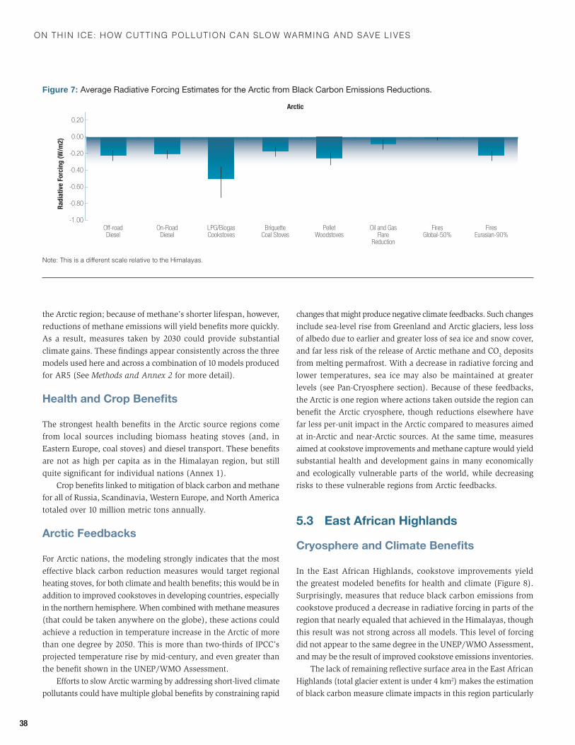
On thin ice: hOw cutting pOllutiOn can slOw warming and save lives
38
the Arctic region; because of methane’s shorter lifespan, however, reductions of methane emissions will yield benefits more quickly. As a result, measures taken by 2030 could provide substantial climate gains. These findings appear consistently across the three models used here and across a combination of 10 models produced for AR5 (See Methods and Annex 2 for more detail).
Health and Crop Benefits
The strongest health benefits in the Arctic source regions come from local sources including biomass heating stoves (and, in Eastern Europe, coal stoves) and diesel transport. These benefits are not as high per capita as in the Himalayan region, but still quite significant for individual nations (Annex 1).
Crop benefits linked to mitigation of black carbon and methane for all of Russia, Scandinavia, Western Europe, and North America totaled over 10 million metric tons annually.
Arctic Feedbacks
For Arctic nations, the modeling strongly indicates that the most effective black carbon reduction measures would target regional heating stoves, for both climate and health benefits; this would be in addition to improved cookstoves in developing countries, especially in the northern hemisphere. When combined with methane measures (that could be taken anywhere on the globe), these actions could achieve a reduction in temperature increase in the Arctic of more than one degree by 2050. This is more than two-thirds of IPCC’s projected temperature rise by mid-century, and even greater than the benefit shown in the UNEP/WMO Assessment.
Efforts to slow Arctic warming by addressing short-lived climate pollutants could have multiple global benefits by constraining rapid
changes that might produce negative climate feedbacks. Such changes include sea-level rise from Greenland and Arctic glaciers, less loss of albedo due to earlier and greater loss of sea ice and snow cover, and far less risk of the release of Arctic methane and CO2 deposits from melting permafrost. With a decrease in radiative forcing and lower temperatures, sea ice may also be maintained at greater levels (see Pan-Cryosphere section). Because of these feedbacks, the Arctic is one region where actions taken outside the region can benefit the Arctic cryosphere, though reductions elsewhere have far less per-unit impact in the Arctic compared to measures aimed at in-Arctic and near-Arctic sources. At the same time, measures aimed at cookstove improvements and methane capture would yield substantial health and development gains in many economically and ecologically vulnerable parts of the world, while decreasing risks to these vulnerable regions from Arctic feedbacks.
5.3 East African Highlands
Cryosphere and Climate Benefits
In the East African Highlands, cookstove improvements yield the greatest modeled benefits for health and climate (Figure 8). Surprisingly, measures that reduce black carbon emissions from cookstove produced a decrease in radiative forcing in parts of the region that nearly equaled that achieved in the Himalayas, though this result was not strong across all models. This level of forcing did not appear to the same degree in the UNEP/WMO Assessment, and may be the result of improved cookstove emissions inventories.
The lack of remaining reflective surface area in the East African Highlands (total glacier extent is under 4 km2) makes the estimation of black carbon measure climate impacts in this region particularly
Figure 7: Average Radiative Forcing Estimates for the Arctic from Black Carbon Emissions Reductions.
Radi
ativ
e Fo
rcin
g (W
/m2)
-0.40
-0.20
0.00
0.20
-1.00
-0.80
-0.60
Arctic
Off-roadDiesel
On-RoadDiesel
LPG/BiogasCookstoves
BriquetteCoal Stoves
PelletWoodstoves
Oil and GasFlare
Reduction
FiresGlobal-50%
FiresEurasian-90%
note: this is a different scale relative to the himalayas.
CryosPhere BenefIts: where health and ClImate InterseCt
39
difficult. Estimates of radiative forcing changes have much higher margins of error, although results across the models were largely consistent (Figure A2–A4). Cookstoves using the Bond et al. assump-tions had especially large error ranges in terms of radiative forcing
(although they still showed benefits consistent with the other models). A multitude of additional complex factors less related to East African black carbon emissions per se, such as the South Asian monsoon, instead appear to drive climate change in the region.
Box 4: Modeled Benefits in the East African Highlands
east africa includes many developing nations with high rural populations, with implementation of clean cooking and sustainable agricultural practices representing serious development challenges. Measures to reduce methane and black carbon brought high health benefits, espe-cially from cookstoves measures, but climate benefits to the small and receding cryosphere proved difficult to capture from modeling alone.
Cryosphere/Climate* Benefits:
• total decrease in radiative forcing, all measures: –1.5 w/m2 (+0.4 to –3.4)• decrease in radiative forcing black carbon measures: –1.2 w/m2 (+0.7 to –3.1)• decrease in radiative forcing from methane measures: –0.32 w/m2
• annual avoided temperature increase from methane measures: about 0.25° C(Note global average anthropogenic radiative forcing is approximately 2.3 W/m2)
Health** and Agricultural Benefits in East African Highlands Source Region:
• annual premature mortality avoided: 123,100• annual increase in staple crops: 153,000 metric tons
Greatest black carbon climate and health benefits: cookstoves (health and climate), open burning (health) and on-road/off-road diesel (climate)
Greatest methane benefits: oil and gas, coal mines, landfills (85%)
* Climate benefits are presented in units of decreased radiative forcing averaged over the region of interest. For comparison, globally averaged anthropogenic forcing from ar5 is 2.3 w/m2; while this regional average does not compare directly with a global average, it is noted to provide a sense of scale compared to the total warming across the globe. ** The public health benefits listed here refer only to the premature mortality avoided due to reductions in ambient (outdoor) air pollution. Some of the measures (principally cookstoves) would also have a significant impact on household (indoor and immediately surrounding the home). This avoided household/indoor exposure is not included in the health benefits estimated above Text Box 2 explores how improved tools would enable estimates of additional benefits due to the impact of reductions on household air quality.
Figure 8: Average Radiative Forcing Estimates for East Africa from Black Carbon Emissions Reductions
Radi
ativ
e Fo
rcin
g (W
/m2 )
-0.40
-0.20
0.00
0.20
-1.00
-0.80
-0.60
East Africa
Off-roadDiesel
On-RoadDiesel
LPG/BiogasCookstoves
BriquetteCoal Stoves
PelletWoodstoves
Oil and GasFlare
Reduction
Fires Global-50%
FiresEurasian-90%
Note: Error bar for cookstove measure extends down to –1.97 W/m2.
On thin ice: hOw cutting pOllutiOn can slOw warming and save lives
40
Health and Crop Benefits
The number of avoided deaths in the source region affecting the East African Highlands is second only to the Himalayas and is far greater as a percentage of the population in the region due to more widespread use of biomass for cooking among rural and urban populations. Total cookstove-related avoided premature deaths from outdoor air pollution were around 94,000; with indoor (household) exposure included, the number of annual avoided deaths related to cookstoves measures might prove more than twice as large. Crop benefits totaled about 153,000 metric tons.
The most compelling reason to implement black carbon and methane reduction measures in the East African Highlands clearly falls on the health and development side, with a decrease in radia-tive forcing providing a desirable, but somewhat uncertain, co-benefit. The gains from improved cookstoves—in terms of health, safety and advances to the well-being and status of women and girls—highlight for municipal authorities and national governments the importance of taking this action.
5.4 Andes and Patagonia
Cryosphere and Climate Benefits
Characterizing the potential gains for the Andes and Patago-nia with any degree of certainty proved difficult due to the extremely thin north-south extent of this alpine range. At its widest point in Chile and Argentina, the Andean range is only 200 kilometers—narrower than the 2.5 degrees (around 270 km) spanned by global climate models. (Out of necessity, some of the modeled area included open ocean. See Figure 5.) Existing cryosphere in the Northern Andes is limited to a few peaks today, similar to the East African highlands (though annual snow and glacier cover in Ecuador is still greater than that at the latitudinal equivalent point in East Africa.) This lack of reflective surface may be part of the reason behind the extremely weak radiative forcing results, which in some cases (biomass burning) indicated slight increases in radiative forcing from the measures (Figure 9).
Andean glaciers have disappeared at faster documented rates than almost anywhere else on the globe. Efforts to preserve them have a great degree of urgency due to the population’s depen-dence on snow and glacier runoff for water supplies, including for agricultural irrigation. Improved regional models should help to ascertain whether cuts in black carbon sources can indeed help to preserve glaciers and mitigate regional climate change.
A more rapid and effective approach might involve observa-tional studies to define the amounts of black carbon reaching the
glaciers and snow pack in order to see whether concentrations are sufficiently significant to motivate early action to reduce emissions given the highly localized impact of black carbon and differing dependency on glacier and snow melt runoff for local populations. In one section of the Peruvian Andes, for example, a recent study showed local communities to be extremely dependent on melt water during the dry season. Both
Box 5: Modeled Benefits in the Andes and Patagonia
The Andes include a mix of urban and rural populations, with much of the rural population living in the mountainous regions or nearby regions of pampas and jungle. development challenges include air quality issues, especially in urban areas with pollution linked to diesel consumption and the use of cookstoves. open burning also is a widespread practice.
Cryosphere/Climate* Benefits:
• total decrease in radiative forcing, all measures: –0.6 w/m2 (–0.2 to –1.0)
• decrease in radiative forcing from black carbon reduction measures: –0.3 w/m2 (+0.1 to –0.7)
• decrease in radiative forcing from methane reduction mea-sures: –0.32 w/m2
• annual avoided temperature increase from methane reduc-tion measures: about 0.25° C
(Note global average anthropogenic radiative forcing is approxi-mately 2.3 w/m2)
Health** and Agricultural Benefits in the Andean Source Region:
• annual premature mortality avoided: 27,000• annual increase in staple crops: 2.6 metric tons***
Greatest black carbon benefits: cookstoves, on-road/off-road diesel
Greatest methane benefits: oil and gas, coal mines, landfills (85 percent)
* Climate benefits are presented in units of decreased radiative forcing averaged over the region of interest. for comparison, globally averaged anthropogenic forcing from ar5 is 2.3 w/m2; while this regional average does not compare directly with a global average, it is noted to provide a sense of scale compared to the total warming across the globe.** The public health benefits listed here refer only to the premature mortality avoided due to reductions in ambient (outdoor) air pollution. Some of the measures (principally cookstoves) would also have a significant impact on household (indoor and immediately surrounding the home). This avoided household/indoor exposure is not included in the health benefits estimated above. Text Box 2 explores how improved tools would enable estimates of additional benefits due to the impact of reductions on household air quality.*** refers to all of south america
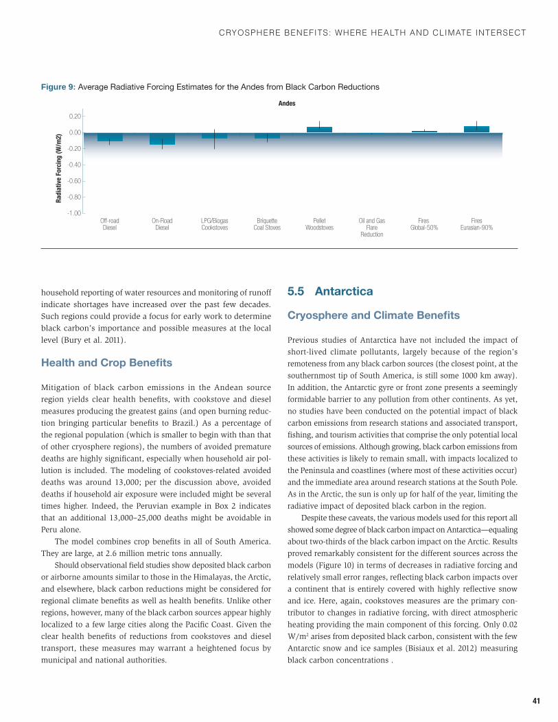
CryosPhere BenefIts: where health and ClImate InterseCt
41
household reporting of water resources and monitoring of runoff indicate shortages have increased over the past few decades. Such regions could provide a focus for early work to determine black carbon’s importance and possible measures at the local level (Bury et al. 2011).
Health and Crop Benefits
Mitigation of black carbon emissions in the Andean source region yields clear health benefits, with cookstove and diesel measures producing the greatest gains (and open burning reduc-tion bringing particular benefits to Brazil.) As a percentage of the regional population (which is smaller to begin with than that of other cryosphere regions), the numbers of avoided premature deaths are highly significant, especially when household air pol-lution is included. The modeling of cookstoves-related avoided deaths was around 13,000; per the discussion above, avoided deaths if household air exposure were included might be several times higher. Indeed, the Peruvian example in Box 2 indicates that an additional 13,000–25,000 deaths might be avoidable in Peru alone.
The model combines crop benefits in all of South America. They are large, at 2.6 million metric tons annually.
Should observational field studies show deposited black carbon or airborne amounts similar to those in the Himalayas, the Arctic, and elsewhere, black carbon reductions might be considered for regional climate benefits as well as health benefits. Unlike other regions, however, many of the black carbon sources appear highly localized to a few large cities along the Pacific Coast. Given the clear health benefits of reductions from cookstoves and diesel transport, these measures may warrant a heightened focus by municipal and national authorities.
5.5 Antarctica
Cryosphere and Climate Benefits
Previous studies of Antarctica have not included the impact of short-lived climate pollutants, largely because of the region’s remoteness from any black carbon sources (the closest point, at the southernmost tip of South America, is still some 1000 km away). In addition, the Antarctic gyre or front zone presents a seemingly formidable barrier to any pollution from other continents. As yet, no studies have been conducted on the potential impact of black carbon emissions from research stations and associated transport, fishing, and tourism activities that comprise the only potential local sources of emissions. Although growing, black carbon emissions from these activities is likely to remain small, with impacts localized to the Peninsula and coastlines (where most of these activities occur) and the immediate area around research stations at the South Pole. As in the Arctic, the sun is only up for half of the year, limiting the radiative impact of deposited black carbon in the region.
Despite these caveats, the various models used for this report all showed some degree of black carbon impact on Antarctica—equaling about two-thirds of the black carbon impact on the Arctic. Results proved remarkably consistent for the different sources across the models (Figure 10) in terms of decreases in radiative forcing and relatively small error ranges, reflecting black carbon impacts over a continent that is entirely covered with highly reflective snow and ice. Here, again, cookstoves measures are the primary con-tributor to changes in radiative forcing, with direct atmospheric heating providing the main component of this forcing. Only 0.02 W/m2 arises from deposited black carbon, consistent with the few Antarctic snow and ice samples (Bisiaux et al. 2012) measuring black carbon concentrations .
Figure 9: Average Radiative Forcing Estimates for the Andes from Black Carbon Reductions
Radi
ativ
e Fo
rcin
g (W
/m2)
-0.40
-0.20
0.00
0.20
-1.00
-0.80
-0.60
Andes
Off-roadDiesel
On-RoadDiesel
LPG/BiogasCookstoves
BriquetteCoal Stoves
PelletWoodstoves
Oil and GasFlare
Reduction
Fires Global-50%
FiresEurasian-90%
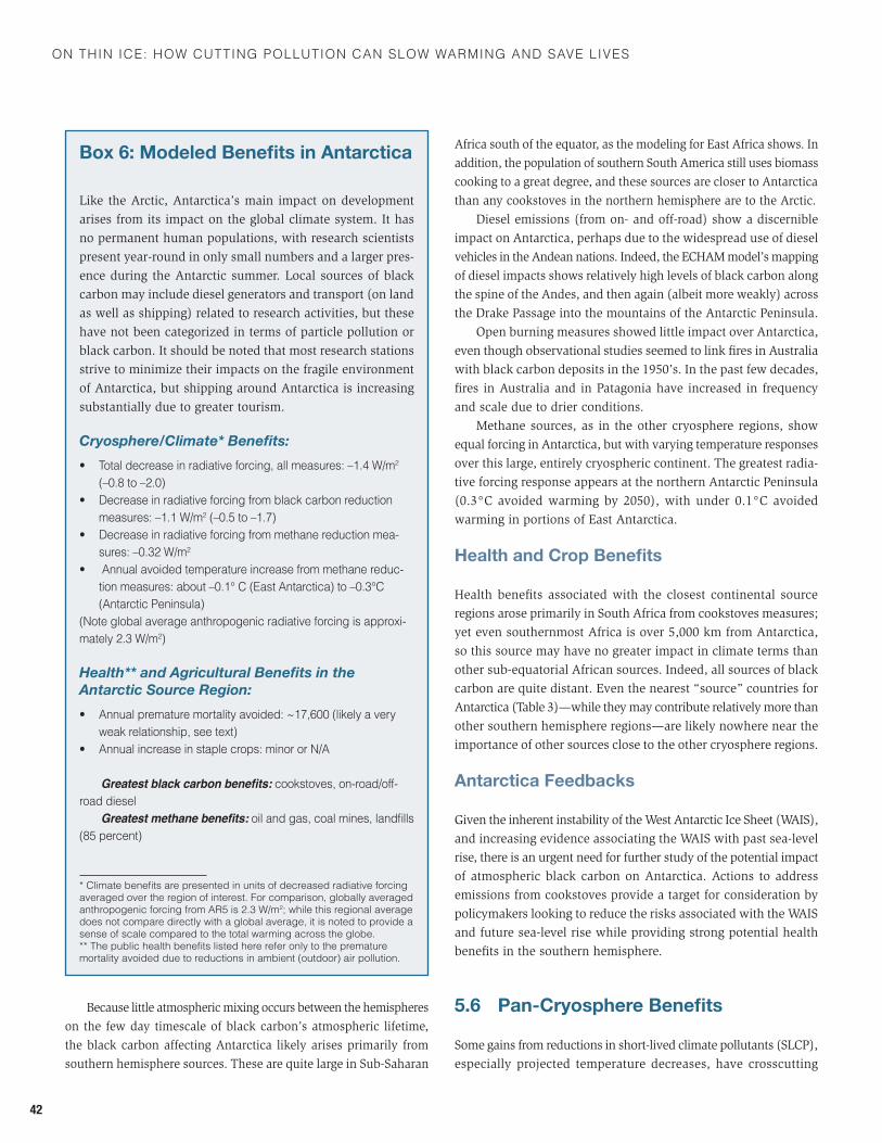
On thin ice: hOw cutting pOllutiOn can slOw warming and save lives
42
Because little atmospheric mixing occurs between the hemispheres on the few day timescale of black carbon’s atmospheric lifetime, the black carbon affecting Antarctica likely arises primarily from southern hemisphere sources. These are quite large in Sub-Saharan
Africa south of the equator, as the modeling for East Africa shows. In addition, the population of southern South America still uses biomass cooking to a great degree, and these sources are closer to Antarctica than any cookstoves in the northern hemisphere are to the Arctic.
Diesel emissions (from on- and off-road) show a discernible impact on Antarctica, perhaps due to the widespread use of diesel vehicles in the Andean nations. Indeed, the ECHAM model’s mapping of diesel impacts shows relatively high levels of black carbon along the spine of the Andes, and then again (albeit more weakly) across the Drake Passage into the mountains of the Antarctic Peninsula.
Open burning measures showed little impact over Antarctica, even though observational studies seemed to link fires in Australia with black carbon deposits in the 1950’s. In the past few decades, fires in Australia and in Patagonia have increased in frequency and scale due to drier conditions.
Methane sources, as in the other cryosphere regions, show equal forcing in Antarctica, but with varying temperature responses over this large, entirely cryospheric continent. The greatest radia-tive forcing response appears at the northern Antarctic Peninsula (0.3°C avoided warming by 2050), with under 0.1°C avoided warming in portions of East Antarctica.
Health and Crop Benefits
Health benefits associated with the closest continental source regions arose primarily in South Africa from cookstoves measures; yet even southernmost Africa is over 5,000 km from Antarctica, so this source may have no greater impact in climate terms than other sub-equatorial African sources. Indeed, all sources of black carbon are quite distant. Even the nearest “source” countries for Antarctica (Table 3)—while they may contribute relatively more than other southern hemisphere regions—are likely nowhere near the importance of other sources close to the other cryosphere regions.
Antarctica Feedbacks
Given the inherent instability of the West Antarctic Ice Sheet (WAIS), and increasing evidence associating the WAIS with past sea-level rise, there is an urgent need for further study of the potential impact of atmospheric black carbon on Antarctica. Actions to address emissions from cookstoves provide a target for consideration by policymakers looking to reduce the risks associated with the WAIS and future sea-level rise while providing strong potential health benefits in the southern hemisphere.
5.6 Pan-Cryosphere Benefits
Some gains from reductions in short-lived climate pollutants (SLCP), especially projected temperature decreases, have crosscutting
Box 6: Modeled Benefits in Antarctica
Like the Arctic, Antarctica’s main impact on development arises from its impact on the global climate system. It has no permanent human populations, with research scientists present year-round in only small numbers and a larger pres-ence during the Antarctic summer. Local sources of black carbon may include diesel generators and transport (on land as well as shipping) related to research activities, but these have not been categorized in terms of particle pollution or black carbon. It should be noted that most research stations strive to minimize their impacts on the fragile environment of Antarctica, but shipping around Antarctica is increasing substantially due to greater tourism.
Cryosphere/Climate* Benefits:
• total decrease in radiative forcing, all measures: –1.4 w/m2 (–0.8 to –2.0)
• decrease in radiative forcing from black carbon reduction measures: –1.1 w/m2 (–0.5 to –1.7)
• decrease in radiative forcing from methane reduction mea-sures: –0.32 w/m2
• annual avoided temperature increase from methane reduc-tion measures: about –0.1° C (East Antarctica) to –0.3°C (Antarctic Peninsula)
(Note global average anthropogenic radiative forcing is approxi-mately 2.3 w/m2)
Health** and Agricultural Benefits in the Antarctic Source Region:
• annual premature mortality avoided: ~17,600 (likely a very weak relationship, see text)
• annual increase in staple crops: minor or n/a
Greatest black carbon benefits: cookstoves, on-road/off-road diesel
Greatest methane benefits: oil and gas, coal mines, landfills (85 percent)
* Climate benefits are presented in units of decreased radiative forcing averaged over the region of interest. for comparison, globally averaged anthropogenic forcing from ar5 is 2.3 w/m2; while this regional average does not compare directly with a global average, it is noted to provide a sense of scale compared to the total warming across the globe. ** The public health benefits listed here refer only to the premature mortality avoided due to reductions in ambient (outdoor) air pollution.
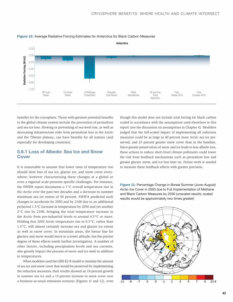
CryosPhere BenefIts: where health and ClImate InterseCt
43
benefits for the cryosphere. Those with greatest potential benefits to the global climate system include the prevention of permafrost and sea ice loss. Slowing or preventing of sea-level rise, as well as decreasing infrastructure risks from permafrost loss in the Arctic and the Tibetan plateau, can have benefits for all nations (and especially for developing countries).
5.6.1 Loss of Albedo: Sea Ice and Snow Cover
It is reasonable to assume that lower rates of temperature rise should slow loss of sea ice, glacier ice, and snow cover every-where; however characterizing these changes at a global or even a regional scale presents specific challenges. For instance, the SWIPA report documents a 1°C overall temperature rise in the Arctic over the past two decades and a decrease in summer minimum sea ice extent of 50 percent. SWIPA predicted such changes to accelerate by 2050 and by 2100 due to an additional projected 1.5°C increase in temperature by 2050 and yet another 2°C rise by 2100, bringing the total temperature increase in the Arctic from pre-industrial levels to around 4.5°C or more. Holding that 2050 Arctic temperature rise to 0.5°C, rather than 1.5°C, will almost certainly increase sea and glacier ice extent as well as snow cover. In mountain areas, the freeze line for glaciers and snow would move to a lower altitude; but the precise degree of these effects needs further investigation. A number of other factors, including precipitation levels and sea currents, also greatly impact the process of snow and ice melt in addition to temperatures.
When modelers used the GISS-E2-R model to simulate the amount of sea ice and snow cover that would be preserved by implementing the reduction measures, their results showed an 18-percent growth in summer sea ice and a 13-percent increase in snow cover over a business-as-usual emissions scenario (Figures 11 and 12), even
though this model does not include total forcing for black carbon scaled in accordance with the assumptions used elsewhere in this report (see the discussion on assumptions in Chapter 4). Modelers judged that the full-scaled impact of implementing all reduction measures could be as large as 40 percent more Arctic sea ice pre-served, and 25 percent greater snow cover than in the baseline. Since greater preservation of snow and ice leads to less albedo loss, these actions to reduce short-lived climate pollutants could lower the risk from feedback mechanisms such as permafrost loss and greater glacier, snow, and ice loss later on. Future work is needed to measure these feedback effects with greater precision.
Figure 10: Average Radiative Forcing Estimates for Antarctica for Black Carbon Measures
Radi
ativ
e Fo
rcin
g (W
/m2)
-0.40
-0.20
0.00
0.20
-1.00
-0.80
-0.60
Antarctica
Off-roadDiesel
On-RoadDiesel
LPG/BiogasCookstoves
BriquetteCoal Stoves
PelletWoodstoves
Oil and GasFlare
Reduction
Fires Global-50%
FiresEurasian-90%
Figure 11: Percentage Change in Boreal Summer (June–August) Arctic Ice Cover in 2050 due to Full Implementation of Methane and Black Carbon Measures by 2030 (unscaled results; scaled results would be approximately two times greater)
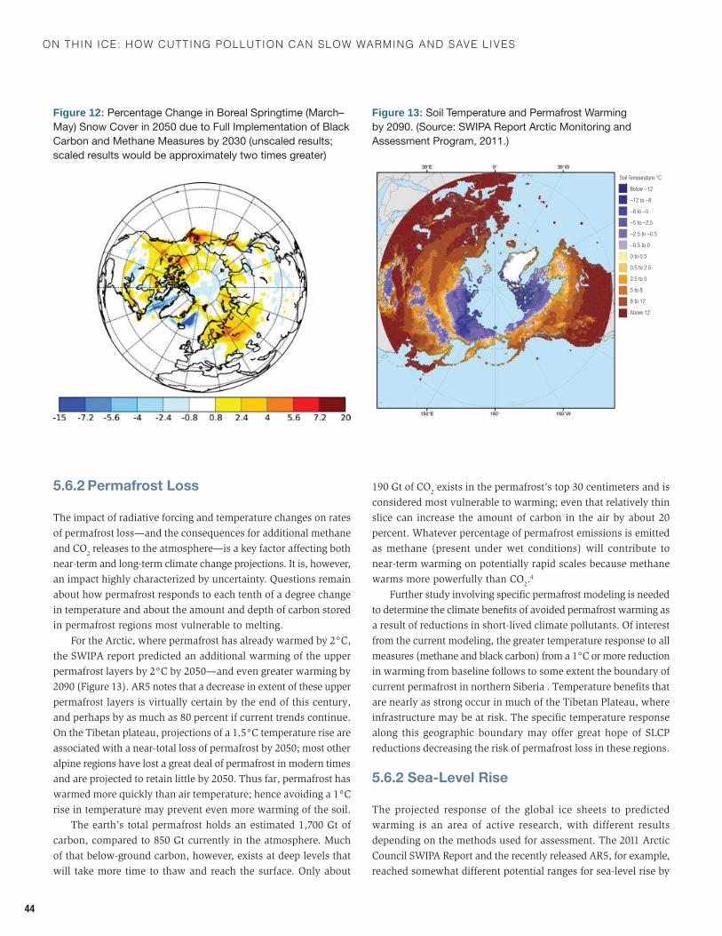
On thin ice: hOw cutting pOllutiOn can slOw warming and save lives
44
5.6.2 Permafrost Loss
The impact of radiative forcing and temperature changes on rates of permafrost loss—and the consequences for additional methane and CO2 releases to the atmosphere—is a key factor affecting both near-term and long-term climate change projections. It is, however, an impact highly characterized by uncertainty. Questions remain about how permafrost responds to each tenth of a degree change in temperature and about the amount and depth of carbon stored in permafrost regions most vulnerable to melting.
For the Arctic, where permafrost has already warmed by 2°C, the SWIPA report predicted an additional warming of the upper permafrost layers by 2°C by 2050—and even greater warming by 2090 (Figure 13). AR5 notes that a decrease in extent of these upper permafrost layers is virtually certain by the end of this century, and perhaps by as much as 80 percent if current trends continue. On the Tibetan plateau, projections of a 1.5°C temperature rise are associated with a near-total loss of permafrost by 2050; most other alpine regions have lost a great deal of permafrost in modern times and are projected to retain little by 2050. Thus far, permafrost has warmed more quickly than air temperature; hence avoiding a 1°C rise in temperature may prevent even more warming of the soil.
The earth’s total permafrost holds an estimated 1,700 Gt of carbon, compared to 850 Gt currently in the atmosphere. Much of that below-ground carbon, however, exists at deep levels that will take more time to thaw and reach the surface. Only about
190 Gt of CO2 exists in the permafrost’s top 30 centimeters and is
considered most vulnerable to warming; even that relatively thin slice can increase the amount of carbon in the air by about 20 percent. Whatever percentage of permafrost emissions is emitted as methane (present under wet conditions) will contribute to near-term warming on potentially rapid scales because methane warms more powerfully than CO2.
4
Further study involving specific permafrost modeling is needed to determine the climate benefits of avoided permafrost warming as a result of reductions in short-lived climate pollutants. Of interest from the current modeling, the greater temperature response to all measures (methane and black carbon) from a 1°C or more reduction in warming from baseline follows to some extent the boundary of current permafrost in northern Siberia . Temperature benefits that are nearly as strong occur in much of the Tibetan Plateau, where infrastructure may be at risk. The specific temperature response along this geographic boundary may offer great hope of SLCP reductions decreasing the risk of permafrost loss in these regions.
5.6.2 Sea-Level Rise
The projected response of the global ice sheets to predicted warming is an area of active research, with different results depending on the methods used for assessment. The 2011 Arctic Council SWIPA Report and the recently released AR5, for example, reached somewhat different potential ranges for sea-level rise by
Figure 12: Percentage Change in Boreal Springtime (March–May) Snow Cover in 2050 due to Full Implementation of Black Carbon and Methane Measures by 2030 (unscaled results; scaled results would be approximately two times greater)
Figure 13: Soil Temperature and Permafrost Warming by 2090. (Source: SWIPA Report Arctic Monitoring and Assessment Program, 2011.)
Soil Temperature °C
Below –12
–12 to –8
–8 to –5
–5 to –2.5
–2.5 to –0.5
–0.5 to 0
0 to 0.5
0.5 to 2.5
2.5 to 5
5 to 8
8 to 12
Above 12
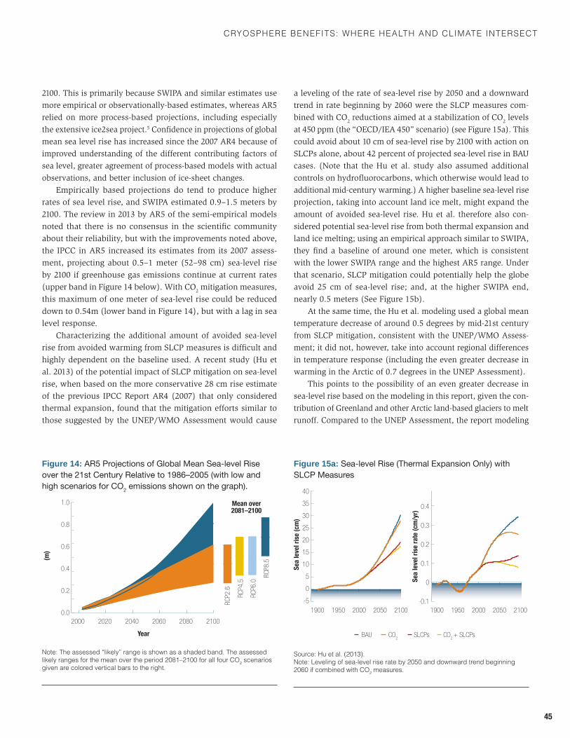
CryosPhere BenefIts: where health and ClImate InterseCt
45
2100. This is primarily because SWIPA and similar estimates use more empirical or observationally-based estimates, whereas AR5 relied on more process-based projections, including especially the extensive ice2sea project.5 Confidence in projections of global mean sea level rise has increased since the 2007 AR4 because of improved understanding of the different contributing factors of sea level, greater agreement of process-based models with actual observations, and better inclusion of ice-sheet changes.
Empirically based projections do tend to produce higher rates of sea level rise, and SWIPA estimated 0.9–1.5 meters by 2100. The review in 2013 by AR5 of the semi-empirical models noted that there is no consensus in the scientific community about their reliability, but with the improvements noted above, the IPCC in AR5 increased its estimates from its 2007 assess-ment, projecting about 0.5–1 meter (52–98 cm) sea-level rise by 2100 if greenhouse gas emissions continue at current rates (upper band in Figure 14 below). With CO2 mitigation measures, this maximum of one meter of sea-level rise could be reduced down to 0.54m (lower band in Figure 14), but with a lag in sea level response.
Characterizing the additional amount of avoided sea-level rise from avoided warming from SLCP measures is difficult and highly dependent on the baseline used. A recent study (Hu et al. 2013) of the potential impact of SLCP mitigation on sea-level rise, when based on the more conservative 28 cm rise estimate of the previous IPCC Report AR4 (2007) that only considered thermal expansion, found that the mitigation efforts similar to those suggested by the UNEP/WMO Assessment would cause
a leveling of the rate of sea-level rise by 2050 and a downward trend in rate beginning by 2060 were the SLCP measures com-bined with CO2 reductions aimed at a stabilization of CO2 levels at 450 ppm (the “OECD/IEA 450” scenario) (see Figure 15a). This could avoid about 10 cm of sea-level rise by 2100 with action on SLCPs alone, about 42 percent of projected sea-level rise in BAU cases. (Note that the Hu et al. study also assumed additional controls on hydrofluorocarbons, which otherwise would lead to additional mid-century warming.) A higher baseline sea-level rise projection, taking into account land ice melt, might expand the amount of avoided sea-level rise. Hu et al. therefore also con-sidered potential sea-level rise from both thermal expansion and land ice melting; using an empirical approach similar to SWIPA, they find a baseline of around one meter, which is consistent with the lower SWIPA range and the highest AR5 range. Under that scenario, SLCP mitigation could potentially help the globe avoid 25 cm of sea-level rise; and, at the higher SWIPA end, nearly 0.5 meters (See Figure 15b).
At the same time, the Hu et al. modeling used a global mean temperature decrease of around 0.5 degrees by mid-21st century from SLCP mitigation, consistent with the UNEP/WMO Assess-ment; it did not, however, take into account regional differences in temperature response (including the even greater decrease in warming in the Arctic of 0.7 degrees in the UNEP Assessment).
This points to the possibility of an even greater decrease in sea-level rise based on the modeling in this report, given the con-tribution of Greenland and other Arctic land-based glaciers to melt runoff. Compared to the UNEP Assessment, the report modeling
Figure 14: AR5 Projections of Global Mean Sea-level Rise over the 21st Century Relative to 1986–2005 (with low and high scenarios for CO2 emissions shown on the graph).
(m)
0.4
0.6
0.8
1.0
0.0
0.2
Year
2000 2080206020402020 2100
RCP2
.6
RCP4
.5
RCP6
.0
RCP8
.5
Mean over2081–2100
Note: The assessed “likely” range is shown as a shaded band. The assessed likely ranges for the mean over the period 2081–2100 for all four Co2 scenarios given are colored vertical bars to the right.
Figure 15a: Sea-level Rise (Thermal Expansion Only) with SLCP Measures
Sea
leve
l ris
e (c
m)
25
30
35
40
5
10
15
20
0
1900 2100205020001950
Sea
leve
l ris
e ra
te (c
m/y
r)
BAU CO2
SLCPs CO2 + SLCPs
-5 -0.1
0
0.1
0.2
0.3
0.4
1900 2100205020001950
Source: Hu et al. (2013). note: leveling of sea-level rise rate by 2050 and downward trend beginning 2060 if combined with Co2 measures.
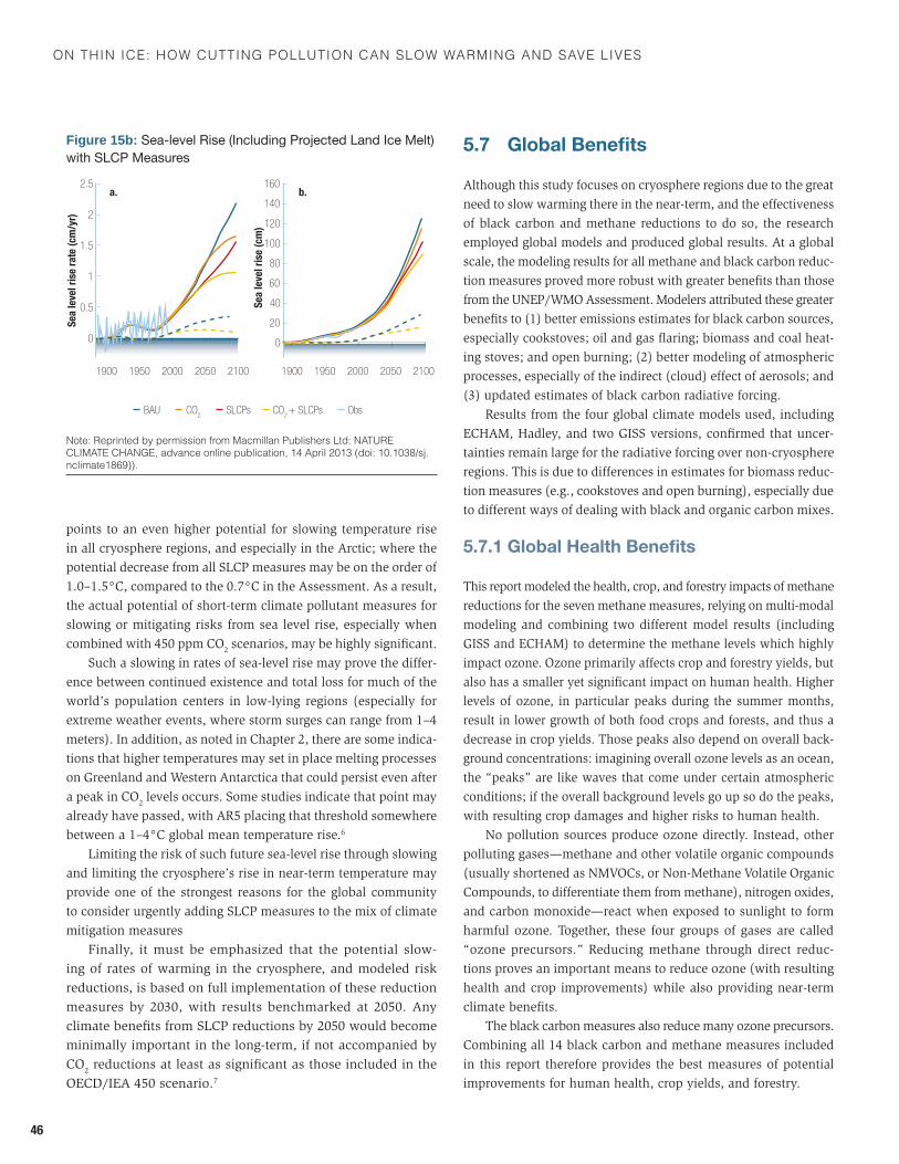
On thin ice: hOw cutting pOllutiOn can slOw warming and save lives
46
points to an even higher potential for slowing temperature rise in all cryosphere regions, and especially in the Arctic; where the potential decrease from all SLCP measures may be on the order of 1.0–1.5°C, compared to the 0.7°C in the Assessment. As a result, the actual potential of short-term climate pollutant measures for slowing or mitigating risks from sea level rise, especially when combined with 450 ppm CO2 scenarios, may be highly significant.
Such a slowing in rates of sea-level rise may prove the differ-ence between continued existence and total loss for much of the world’s population centers in low-lying regions (especially for extreme weather events, where storm surges can range from 1–4 meters). In addition, as noted in Chapter 2, there are some indica-tions that higher temperatures may set in place melting processes on Greenland and Western Antarctica that could persist even after a peak in CO2 levels occurs. Some studies indicate that point may already have passed, with AR5 placing that threshold somewhere between a 1–4°C global mean temperature rise.6
Limiting the risk of such future sea-level rise through slowing and limiting the cryosphere’s rise in near-term temperature may provide one of the strongest reasons for the global community to consider urgently adding SLCP measures to the mix of climate mitigation measures
Finally, it must be emphasized that the potential slow-ing of rates of warming in the cryosphere, and modeled risk reductions, is based on full implementation of these reduction measures by 2030, with results benchmarked at 2050. Any climate benefits from SLCP reductions by 2050 would become minimally important in the long-term, if not accompanied by CO2 reductions at least as significant as those included in the OECD/IEA 450 scenario.7
5.7 Global Benefits
Although this study focuses on cryosphere regions due to the great need to slow warming there in the near-term, and the effectiveness of black carbon and methane reductions to do so, the research employed global models and produced global results. At a global scale, the modeling results for all methane and black carbon reduc-tion measures proved more robust with greater benefits than those from the UNEP/WMO Assessment. Modelers attributed these greater benefits to (1) better emissions estimates for black carbon sources, especially cookstoves; oil and gas flaring; biomass and coal heat-ing stoves; and open burning; (2) better modeling of atmospheric processes, especially of the indirect (cloud) effect of aerosols; and (3) updated estimates of black carbon radiative forcing.
Results from the four global climate models used, including ECHAM, Hadley, and two GISS versions, confirmed that uncer-tainties remain large for the radiative forcing over non-cryosphere regions. This is due to differences in estimates for biomass reduc-tion measures (e.g., cookstoves and open burning), especially due to different ways of dealing with black and organic carbon mixes.
5.7.1 Global Health Benefits
This report modeled the health, crop, and forestry impacts of methane reductions for the seven methane measures, relying on multi-modal modeling and combining two different model results (including GISS and ECHAM) to determine the methane levels which highly impact ozone. Ozone primarily affects crop and forestry yields, but also has a smaller yet significant impact on human health. Higher levels of ozone, in particular peaks during the summer months, result in lower growth of both food crops and forests, and thus a decrease in crop yields. Those peaks also depend on overall back-ground concentrations: imagining overall ozone levels as an ocean, the “peaks” are like waves that come under certain atmospheric conditions; if the overall background levels go up so do the peaks, with resulting crop damages and higher risks to human health.
No pollution sources produce ozone directly. Instead, other polluting gases—methane and other volatile organic compounds (usually shortened as NMVOCs, or Non-Methane Volatile Organic Compounds, to differentiate them from methane), nitrogen oxides, and carbon monoxide—react when exposed to sunlight to form harmful ozone. Together, these four groups of gases are called “ozone precursors.” Reducing methane through direct reduc-tions proves an important means to reduce ozone (with resulting health and crop improvements) while also providing near-term climate benefits.
The black carbon measures also reduce many ozone precursors. Combining all 14 black carbon and methane measures included in this report therefore provides the best measures of potential improvements for human health, crop yields, and forestry.
Figure 15b: Sea-level Rise (Including Projected Land Ice Melt) with SLCP Measures
Sea
leve
l ris
e (c
m)
1
1.5
2
2.5
0
0.5
a.
1900 2100205020001950
Sea
leve
l ris
e ra
te (c
m/y
r)
BAU CO2
SLCPs CO2 + SLCPs
60
80
100
120
140
160
1900 2100205020001950
b.
20
40
0
Obs
note: reprinted by permission from macmillan Publishers ltd: natUre ClImate ChanGe, advance online publication, 14 april 2013 (doi: 10.1038/sj. nclimate1869)).
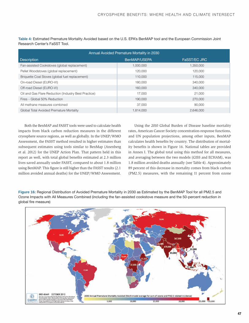
CryosPhere BenefIts: where health and ClImate InterseCt
47
Both the BenMAP and FASST tools were used to calculate health impacts from black carbon reduction measures in the different cryosphere source regions, as well as globally. In the UNEP/WMO Assessment, the FASST method resulted in higher estimates than subsequent estimates using tools similar to BenMap (Anenberg et al. 2012) for the UNEP Action Plan. That pattern held in this report as well, with total global benefits estimated at 2.3 million lives saved annually under FASST, compared to about 1.8 million using BenMAP. This figure is still higher than the FASST results (2.1 million avoided annual deaths) for the UNEP/WMO Assessment.
Using the 2010 Global Burden of Disease baseline mortality rates, American Cancer Society concentration-response functions, and UN population projections, among other inputs, BenMAP calculates health benefits by country. The distribution of mortal-ity benefits is shown in Figure 16. National tables are provided in Annex I. The global total using this method for all measures, and averaging between the two models (GISS and ECHAM), was 1.8 million avoided deaths annually (see Table 4). Approximately 89 percent of this decrease in mortality comes from black carbon (PM2.5) measures, with the remaining 11 percent from ozone
Table 4: Estimated Premature Mortality Avoided based on the U.S. EPA’s BenMAP tool and the European Commission Joint Research Center’s FaSST Tool.
Annual Avoided Premature Mortality in 2030
Description BenMAP/USEPA FaSST/EC JRCFan-assisted Cookstoves (global replacement) 1,000,000 1,350,000Pellet Woodstoves (global replacement) 120,000 120,000Briquette Coal Stoves (global fuel replacement) 110,000 115,000On-road Diesel (EURO-VI) 180,000 340,000Off-road Diesel (EURO-VI) 160,000 340,000Oil and Gas Flare Reduction (Industry Best Practice) 17,000 21,000fires – Global 50% reduction 190,000 270,000all methane measures combined 37,000 90,000Global total avoided Premature mortality 1,814,000 2,646,000
Figure 16: Regional Distribution of Avoided Premature Mortality in 2030 as Estimated by the BenMAP Tool for all PM2.5 and Ozone Impacts with All Measures Combined (including the fan-assisted cookstove measure and the 50-percent reduction in globalfiremeasure)
On thin ice: hOw cutting pOllutiOn can slOw warming and save lives
48
impacts primarily related to the methane measures (but also includ-ing other ozone precursors arising from black carbon reductions).
Deploying advanced cookstoves provided for over half the number of overall avoided deaths. The GBD has estimated total deaths from cookstoves at four million if deaths from household level (indoor) smoke exposure are included. This means the likely total benefit from implementation of all SLCP reduction measures could be far higher if all premature deaths from cookstoves, including household-level smoke exposure, are included. Better quantifying this potential will require more regionally based work such as that outlined in Box 2; but it clearly is quite large.
It is notable that recent studies have associated the smallest of particles—smaller even than PM2.5, which includes black car-bon—with the most severe effects from local particle pollution, especially diesel (International Agency for Research on Cancer 2012).
Researchers have speculated that these smallest “carbonaceous particles” fasten deeper in the lungs, proving difficult to cough out; bind more toxic substance; and more-easily cross the barrier between the lungs and the bloodstream. This may mean that the same actions designed from a black carbon reduction standpoint may also prove effective in improving human health.
5.7.2 Global Crop and Forestry Benefits
FASST was used to calculate the impact of the emissions reduc-tion measures on agricultural yields due to decreases in ozone pollution. Impacts on crops arise from all methane emissions (see Table 5), though decreases in ozone also result from black carbon measures (and especially diesel). The potential crop yield increase with all methane measures combined was more than 12 million metric tons annually, and the total for all measures was 31 million metric tons. The benefits in China alone exceeded seven million metric tons annually from all measures.
Although much of these benefits come from methane impacts spread more evenly across the globe, per the discus-sion above the black carbon measures producing ozone pre-cursors—especially, diesel use—have much more of a local impact on crops. The greatest crop benefits therefore arise in regions with large potential diesel reductions, due primarily to reductions in associated nitrogen oxide emissions. The two diesel measures each increased the total yield of the four staple crops by around 7–9 million tons annually. Owing to the carbon monoxide emissions from cookstoves, that control measure also provided substantial crop yield benefits of approximately 1.5-–2 million tons annually.
The benefits were highest in regions with the greatest cur-rent diesel emissions. For example, the increase in crop yield due to on-road diesel measures exceeded five million tons in South
Asia (including India), nearly four million tons in China, over two million tons in Latin America, and over one million tons in Southeast Asia. Benefits to crop yields were also substantial in North America, at over three million tons, with two-thirds of that amount arising from methane reduction measures.
Potential forest and timber yield impacts may also be signifi-cant. While methods are under development (Box 7), the analysis indicates results that are extremely species-specific and regional in nature. Further research into these impacts is important, given the contribution of the forestry industry to developing and OECD countries and the key role played by forests in REDD and as a sink for mitigation of greenhouse gases.
5.7.3 Global Climate Benefits
MethaneAs a globally well-mixed gas, methane reductions anywhere decrease methane concentrations in the atmosphere almost evenly across the globe. As a result, the decrease in radiative forcing from all of the modeled methane measures is approximately an even –0.32 W/m2 throughout the globe. The temperature and climate impacts are, however, far less uniform, with land and cryosphere regions—especially in the Arctic—showing far greater benefits: 2–3 times the global mean in the Arctic, and 50-percent greater in much of Antarctica and the Himalayas. This is reflected in the regional information above and shown globally in Figure 17.
Table 5: Annual Increase in the Yield of Four Staple Crops (Wheat, Rice, Maize and Soybean) Due to the Surface Ozone Change Associated with each Black Carbon Measure and All Methane Measures Combined
Description
Avoided Crop Losses (metric
tons)LPG/Biogas Cookstoves (global replacement) 1,690,000Fan-assisted Cookstoves (global replacement) 1,810,000Pellet Woodstoves (global replacement) 275,000Briquette Coal Stoves (global fuel replacement) 32,000On-road Diesel (EURO-VI) 9,460,000Off-road Diesel (EURO-VI) 7,130,000oil and Gas flare reduction (Industry Best Prac-tice) 220,000fires – Global 50% reduction 2,480,000all methane measures combined 12,380,000Global total avoided Crop losses (using fan-assisted cookstove measure) 33,787,000
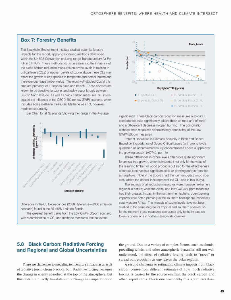
CryosPhere BenefIts: where health and ClImate InterseCt
49
Box 7: Forestry Benefits
the stockholm environment Institute studied potential forestry impacts for this report, applying modeling methods developed within the UneCe Convention on long-range transboundary air Pol-lution (LRTAP). These methods focus on estimating the influence of the black carbon reduction measures on ozone levels in relation to critical levels (CLs) of ozone. Levels of ozone above these CLs may affect the growth of key species in temperate and boreal forests and therefore decrease timber yields. the most well-studied Cls at this time are primarily for european birch and beech. these species are known to be sensitive to ozone, and today occur largely between 35–65° north latitude. as well as black carbon measures, seI inves-tigated the influence of the OECD 450 (or low GWP) scenario, which includes some methane measures. methane was not, however, modeled separately.
Bar Chart for all scenarios showing the range in the average
Difference in the CL Exceedances (2030 Reference—2030 emission scenario) found in the 35–65°N Latitude Bands.
The greatest benefit came from the Low GWP/450ppm scenario, with a combination of Co2 and methane measures that cut ozone
significantly. Three black carbon reduction measures also cut CL exceedance quite significantly: diesel (both on-road and off-road) and a 50-percent decrease in open burning. the combination of these three measures approximately equals that of the Low GwP/450ppm measures.
Percent reduction in Biomass annually in Birch and Beech Based on Exceedance of Ozone Critical Levels (with ozone levels quantified as accumulated hourly concentrations above 40 ppb over the growing season (AOT40; ppm h).
These differences in ozone levels can prove quite significant for annual tree growth, which is important not only for the value of the resulting timber for wood products but also for the effectiveness of forests to serve as a significant sink for drawing carbon from the atmosphere. (note in the above chart the four temperate wood spe-cies, where the dotted lines represent the CL used in this study).
The impacts of all reduction measures were, however, extremely regional in nature; while the diesel and low GWP/450ppm measures had their greatest impact in the northern hemisphere, open burning impacts were noted primarily in the southern hemisphere, especially southwestern Africa. The impacts of ozone levels have not been studied to the same degree for tropical and southern species, so for the moment these measures can speak only to the impact on forestry operations in northern temperate climates.
2
0
-2
-4
-6
4
-8
-10
-12
Diff
eren
ce in
the
CL E
xcee
denc
e (p
pm v
hrs
)
Biofue
l hea
tings
toves
_no s
easo
n
Coal h
eatin
g stov
es_n
o sea
son
Coal h
eatin
g stov
es_s
easo
n
90% Fl
aring
redu
ction
50%
biom
ass b
uring
redu
ction
Low G
WP
On roa
d die
sel
Off roa
d die
sel
Cooks
toves
(fan a
ssiste
d)Br
ick ki
lns
Biofue
l hea
ting s
toves
_sea
son
Emission scenario
% re
duct
ion
10
-10
-20
-30
0
0 20 30 4010
F. sylvatica, CH
B. pendula, Ostad, SE
B. pendula, Kuopio1 , FL
B. pendula, Kuopio2 , FL
B. pendula, Kuopio3 , FL
Birch, beech
Daylight AOT40 (ppm h)
5.8 Black Carbon: Radiative Forcing and Regional and Global Uncertainties
There are challenges to modeling temperature impacts as a result of radiative forcing from black carbon. Radiative forcing measures the change in energy absorbed at the top of the atmosphere, but this does not directly translate into a change in temperature on
the ground. Due to a variety of complex factors, such as clouds, prevailing winds, and other atmospheric dynamics still not well understood, the effect of radiative forcing tends to “move” or spread out, especially as one leaves the polar regions.
A second challenge to estimating climate impacts from black carbon comes from different estimates of how much radiative forcing is caused by the source emitting the black carbon and other co-pollutants. This is one reason why this report uses three
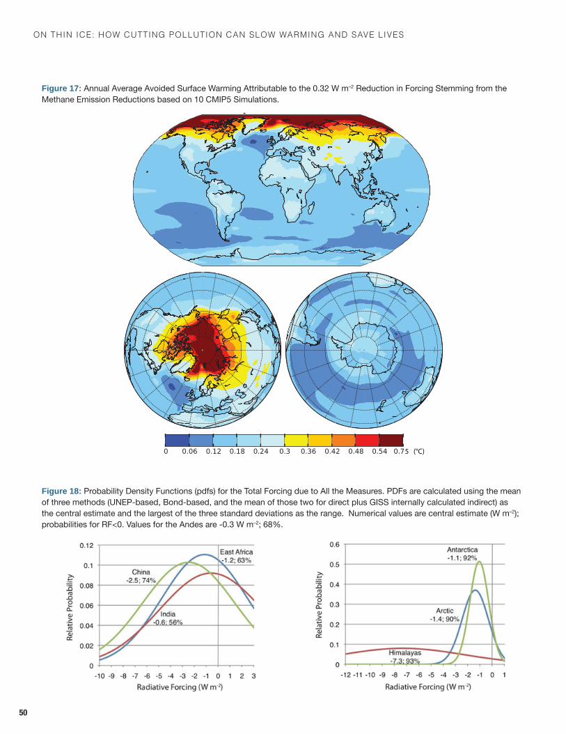
On thin ice: hOw cutting pOllutiOn can slOw warming and save lives
50
Figure 17: Annual Average Avoided Surface Warming Attributable to the 0.32 W m–2 Reduction in Forcing Stemming from the Methane Emission Reductions based on 10 CMIP5 Simulations.
Figure 18: Probability Density Functions (pdfs) for the Total Forcing due to All the Measures. PDFs are calculated using the mean of three methods (UNEP-based, Bond-based, and the mean of those two for direct plus GISS internally calculated indirect) as the central estimate and the largest of the three standard deviations as the range. Numerical values are central estimate (W m–2); probabilities for RF<0. Values for the Andes are -0.3 W m–2; 68%.
5 (°C)
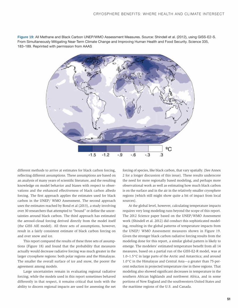
CryosPhere BenefIts: where health and ClImate InterseCt
51
different methods to arrive at estimates for black carbon forcing, reflecting different assumptions. These assumptions are based on an analysis of many years of scientific literature, and the resulting knowledge on model behavior and biases with respect to obser-vations and the enhanced effectiveness of black carbon albedo forcing. The first approach applies the estimates used for black carbon in the UNEP/ WMO Assessment. The second approach uses the estimates reached by Bond et al (2013), a study involving over 30 researchers that attempted to “bound” or define the uncer-tainties around black carbon. The third approach has estimated the aerosol-cloud forcing derived directly from the model itself (the GISS AIE model). All three sets of assumptions, however, result in a fairly consistent estimate of black carbon forcing on and over snow and ice.
This report compared the results of these three sets of assump-tions (Figure 18) and found that the probability that measures actually would decrease radiative forcing was much greater in the larger cryosphere regions: both polar regions and the Himalayas. The smaller the overall surface of ice and snow, the poorer the agreement among models.
Large uncertainties remain in evaluating regional radiative forcing; while the models used in this report sometimes behaved differently in that respect, it remains critical that tools with the ability to discern regional impacts are used for assessing the net
forcing of species, like black carbon, that vary spatially. (See Annex 2 for a longer discussion of this issue). These results underscore the need for more regionally based modeling, and perhaps more observational work as well as estimating how much black carbon is on the surface and in the air in the relatively smaller cryosphere regions (which still might show quite a bit of impact from local sources).
At the global level, however, calculating temperature impacts requires very long modeling runs beyond the scope of this report. The 2012 Science paper based on the UNEP/WMO Assessment work (Shindell et al. 2012) did conduct this sophisticated model-ing, resulting in the global patterns of temperature impacts from the UNEP/ WMO Assessment measures shown in Figure 19. Given the stronger black carbon radiative forcing results from the modeling done for this report, a similar global pattern is likely to emerge. The modelers’ estimated temperature benefit from all 14 measures, based on a partial run of the GISS-E2-R model, was at 1.0–1.5°C in large parts of the Arctic and Antarctica; and around 1.0°C in the Himalayas and Central Asia—a greater than 75-per-cent reduction in projected temperature rise in these regions. That modeling also showed significant decreases in temperature in the southern African highlands and northwest Africa, and in some portions of New England and the southwestern United States and the maritime regions of the U.S. and Canada.
Figure 19: All Methane and Black Carbon UNEP/WMO Assessment Measures. Source: Shindell et al. (2012), using GISS-E2-S. From Simultaneously Mitigating Near-Term Climate Change and Improving Human Health and Food Security. Science 335, 183–189. Reprinted with permission from AAAS
On thin ice: hOw cutting pOllutiOn can slOw warming and save lives
52
Endnotes1 This report makes the following assumptions regarding relative risk of air pollution health impacts which are different than GBD: (i) any amount of PM2.5 has health impacts; (ii) all-cause mortality is used to extrapolate health risk in other parts of the world; and (iii) linear impacts exist at high concentrations. These assumptions could lead to over- or under-estimating the final results. For example, using all-cause mortality could lead to overestimation because relative-risk estimates from the U.S. are extrapo-lated to other parts of the world where people are dying of causes that might not be influenced by air pollution; however, using cause-specific mortality could underestimate impacts because it wouldn’t capture all the mortality causes affected by air pollution, except the major ones—cardiovascular, pulmonary, and lung cancer. Furthermore, the assumption of linear impacts at high concentrations as used in this report compared to the GBD assumption of declining health impacts at high concentrations remains a subject of scientific debate, as does the assumption of an air pollution concentration threshold below which there are no health impacts used in the GBD.2 While this tool has not yet been published, it was reviewed by World Bank expert staff.3 Arctic Council Task Force on Short Lived Climate Forcers (2013).4 IPCC AR5 findings suggest a significant increase in the radiative forcing of methane than was assessed in AR4 (0.47 to 0.98 W/m2) due to impacts by methane on ozone, water vapor, and other emissions that indirectly affect methane.5 See http://www.ice2sea.eu.6 “Sustained mass loss by ice sheets would cause larger sea-level rise, and some part of the mass loss might be irreversible. There is high confidence that sustained warming greater than some threshold would lead to the near-complete loss of the Greenland ice sheet over a millennium or more, causing a global mean sea-level rise of up to 7 m. Current estimates indicate that the threshold is greater than about 1°C (low confidence) but less than about 4°C (medium confidence) global mean warming with respect to pre-industrial levels. Abrupt and irreversible ice loss from a potential instability of marine-based sectors of the Antarctic Ice Sheet in response to climate forcing is pos-sible, but current evidence and understanding is insufficient to make a quantitative assessment.” Working Group I Contribution to the IPCC Fifth Assessment Report (2013).7 See 450 Scenario at www.iea.org.

Chapter 6
55
Discussion: Implications for Sectoral Actions
The abatement measures assessed in this report, like those from the UNEP/WMO Assessment on which it is based, come from a list of sources of pollution and greenhouse
gases. Scientists have identified these reduction measures because, combined with their health and development benefits, these mea-sures1 reduce a mixture of aerosols that can lead to a near-term (by 2050) decrease in radiative forcing and, as this report now shows, slower warming and melting in the cryosphere. Other climate and pollution actions may slow long-term warming or provide important health benefits, or both; but this report focused on exploring those that combine development and near-term, regional cryosphere benefits. While some actions might be con-sidered immediately by policymakers, especially where combined climate and health benefits seem clear, others will require more region and country-specific analysis, including feasibility studies and cost-benefit analyses.
This section looks at sectoral and source-based opportunities to reduce black carbon and methane rather than black carbon and methane impacts in isolation from their sources. The discussion below begins to address some of the policy and operational impli-cations of the different identified sources and sectors, including barriers to adoption.
6.1 Biomass Cookstoves
By far, cookstoves measures emerged as the greatest single source of benefits for health and the cryosphere in the modeling—indicat-ing an opportunity for early and urgent action.
From a cryosphere preservation standpoint, addressing this source provided the largest benefit, from the Himalayas to the Arctic to (rather surprisingly) Antarctica. Most of this benefit arose from direct forcing of black carbon in the atmosphere, which over snow and ice provides a clear degree of radiative forcing. Even though most of the black carbon falls out of the atmosphere much closer to the main source regions, the amount of emissions from cookstoves is so great that even though only a relatively small percentage reaches these cryosphere regions, the
modeling indicates it is still enough to make a measureable impact on radiative forcing in all cryosphere regions.
Cookstoves affect the health of a high percentage of the popu-lation in all three alpine source regions, as well as in countries outside those regions where biomass cookstove use remains high (e.g., Sub-Saharan Africa). It bears noting that health impacts in the Arctic mirrored this health impact for biomass and coal heating stoves: substituting improved heating stoves resulted in nearly 230,000 avoided annual deaths in the Arctic source region (see Table 3 for a definition of source regions).
Nearly three billion people living in developing countries—close to half the world’s population—rely on biomass (wood, charcoal, dung, and crop residues) and coal burning to cook their food and heat their homes; they face daily exposure to smoke. Recent studies (International Agency for Research on Cancer 2012) have found that the tiniest particles within such particulate pollution (smaller than PM2.5), inflict the gravest respiratory damage. Once lodged in the lungs, these superfine particles—which include black carbon/soot—cannot be coughed out, creating the conditions for disease. The Global Burden of Disease estimates that some four million people, mostly women and young children, die prematurely each year from the effects of poorly ventilated household smoke. This toll now exceeds estimates of annual deaths from HIV/AIDS, tuberculosis, and malaria combined.
Demand for wood-fueled energy can have serious negative effects on forests and woodlands where large and sometimes lucra-tive wood-fuel markets create incentives for forest and woodland clearance, or where rural communities depend on fragile ecosystems that are already under environmental stress. In addition, the daily burden of firewood collection contributes to gender inequality, by preventing women and girls from spending time in school or engaged in productive economic activities while exposing them to a higher risk of sexual violence.
Encouragingly, the modeling showed nearly equal health benefits from two different approaches to replacing traditional cookstoves: (1) replacing biomass cookstoves with a 50/50 combination of liquid petroleum gas (LPG) and biogas, which
On thin ice: hOw cutting pOllutiOn can slOw warming and save lives
56
achieved the greatest potential reduction; and (2) from replace-ment by fan-assisted/forced-air biomass cookstoves, at least for outdoor air exposure to stoves pollution (the modeling did not capture household/indoor impacts, which might increase this difference). This flexibility in approach addresses one key barrier to effective cookstoves programs, that of fuel availability options. Although considered a “gold standard” technology, biogas or LPG fuel replacement (or replacement by sustainable production of ethanol, under increasing use in Africa) may not meet the needs of the rural poor. In particular, wood, dung, and grass may prove cheaper or more widely available.
Biogas digesters, which convert manure from cows, pigs, and even human waste to cooking fuel, are commercially available in sizes ranging from a single household to a small village; so are larger installations that gather such waste and distribute the gas. Ethanol provides a third alternative fuel in growing use in Africa, and the health and climate benefits should equal those of LPG and biogas. The ethanol needs to be sustainably produced, however, given competing demands for land and water use for cultivation.
All four cookstove models—LPG, biogas, ethanol, and forced-draft stoves—have been proven to reduce particle pollution and black carbon, but they present different challenges for implementa-tion. Fugitive methane emissions can occur from the two gas-driven stoves; and a badly-maintained or improperly used forced draft stove will emit copious amounts of smoke and black carbon. In addition, all the stoves must be used on a regular basis and main-tained properly to effectively curb pollution emissions. Training, proper maintenance, and long-term monitoring and evaluation must be essential elements of cookstoves replacement programs. Past experience also shows that the sustainability of cookstoves programs is dependent on the sociocultural context, market condi-tions, and affordability (World Bank 2011). Cookstoves designed without the user in mind have often failed; as have programs that lack after-sales services and donor-driven handouts of expensive cookstove models.
Despite these challenges, the costs of continued traditional cookstove use in terms of family health and welfare—not to men-tion the climate impacts—speak to intensified efforts to overcome these barriers and increased “learning by doing;” this is similar to the approach used by donors in the HIV/AIDs, malaria and TB health crisis of the late 1990s. The barriers to distribution and proper use of cookstoves include some striking similarities to the public health challenges of these three infectious diseases: the need to solve issues of distribution (which, for anti-retroviral drugs, included keeping the supply cold throughout the supply chain in rural areas without refrigeration); education in proper use; and ongoing monitoring, evaluation, and follow-up.
Hundreds of public and private initiatives exist to bring cleaner cooking solutions to women across the developing world. These
efforts include commercial and nonprofit enterprises, carbon finance schemes, national and intergovernmental development projects, and humanitarian assistance programs.2 Not all of these programs, however, address emissions in a way that might be expected to bring proven health and climate benefits, with only incremental improvements in emissions levels. As a first step, interventions could perhaps seek to focus these many existing efforts on the four clean cooking solutions proven to maximize those benefits.
Addressing local barriers to improved cookstoves adoption is key, as are affordability and well-designed monitoring and evaluation programs to ensure proper use over time. These four advanced cookstoves perform well (decrease emissions) in labo-ratory conditions, but far more field work in connection with stove replacement programs is needed to ensure that the benefits are realized, endure, and can be replicated. The just-completed pilot phase of Project Surya in India, for example, found that in field testing using forced draft stoves, particle and black carbon emissions were reduced by 60–80 percent.3 However, the cost of advanced cookstoves needs to come down substantially for poor households to be able to afford them.
The World Bank supported, recently announced Government of China’s Clean Stove Initiative (World Bank 2013) is a good example of a cookstove program beginning with a deep understanding of the local country’s household cooking and heating technologies and markets, a review of the existing policies and institutional framework for cooking and heating fuels, and identification of lessons from successful programs that can be applied to promote clean cooking solutions.
6.2 Biomass and Coal Heating Stoves
Modeling of the emission reduction measures for biomass and coal heating stoves improved on previous studies by placing use of these stoves when it most often occurs: during the colder months. This resulted in clearly higher climate impacts in the Arctic and Eastern Himalayas; it also resulted in somewhat higher health impacts in northern Europe where biomass stove use is growing and in parts of Eastern Europe and China for coal stoves.
Rising oil prices, combined with climate change policies aimed at promoting renewable energy over fossil fuels, have contributed to greater use of solid biofuels, especially wood, for household heating. Many recent studies in Europe have associated the grow-ing use of wood heating as a source of winter air pollution—in some cities, such as Berlin, it is becoming the most significant source of particle pollution even when averaged year-round. Wood-burning stoves and fireplaces, as well as boilers, have long played a central role in home heating in Nordic countries. A 2012 study by the International Energy Agency concluded that even in the
dIsCUssIon: ImPlICatIons for seCtoral aCtIons
57
absence of a global climate change agreement, biofuel use in the residential sector will increase (IEA and Norden 2012). Hence there is an urgent need to design and implement an effective approach to limiting black carbon emissions from home heating sources as their use continues to rise.
In addition to the measure modeled for this report—replacement of whole (log) wood biomass stoves by pellet stoves and boilers, which like their forced-draft cookstove counterparts significantly cut emissions of all pollutants (including black carbon)—many countries have extensive experience limiting emissions from wood burning for air quality purposes. Such measures include not only direct regulation, but also consumer incentives to switch to cleaner-burning stoves, voluntary standards (such as the Nordic Swan label),4 and consumer information campaigns on how to use stoves more effectively.
In addition to the modeled measure of fuel replacement by coal briquettes, there have also been successful reductions in China of coal stoves through replacement with LPG or biogas stoves; this usually occurs when such stoves are used more for cooking than heating. Briquettes offer a cost-effective interim solution that can be used in existing stoves.
6.3 Open Burning
The 50-percent decrease in open burning modeled for this report showed little climate impact; it did show, however, surprisingly strong health benefits, ranking it as the second most-effective mitigation measure in health terms (though it still ranks below cookstoves by nearly a factor of 10). This reflects the large amount of particle pollution released as burning occurs, with most health impacts occurring quite close to the source.
Using the “northern Eurasia” option for open burning (90-per-cent decrease) yielded appreciable climate impacts, not just in the Arctic but also in the Himalayas, which borders some extensive seasonal burning in Kazakhstan and Mongolia. This indicates that when open fires are controlled to their greatest extent, not only health but climate benefits could prove quite significant. Outside high altitude and boreal regions, almost all open burning occurs as a result of anthropogenic activities, whether set agricultural or forestry fires or waste or camp fires that grow out of control (Giri and Shrestha 2000; Flannigan et al. 2009).
Introduction of no-burn alternative agricultural methods has resulted in higher yields and profits for many farmers in Western Europe. Public information campaigns to prevent accidental fires can also prove quickly effective. Both measures are relatively inexpensive. Greater exploration of the true reduction potentials for open burning in other regions of the world, beginning with characterization of what is being burned and the motivations behind it, could be a necessary first step.
6.4 Diesel
The greatest benefits from diesel measures—whether aimed at on-road transport or off-road machinery (such as construction and farming equipment)—arose in developing countries where relatively dirty diesel engines without particulate filters are expected to continue to be in wide use through 2030. The Himalayan region showed espe-cially strong impacts from diesel measures, but East Africa and to some degree the Andes also showed benefits both on the health and climate sides. Diesel reduction measures also showed strong benefits using two of the three sets of forcing assumptions in the Arctic, although results were quite weak using the GISS-AIE assumptions.
It bears noting that this measure assumes that all mobile diesel sources would meet EURO-VI standards by 2030 in most OECD countries; as a result, these reductions are not included in the benefits calculations. Some policy decisions that might delay this change—in particular, any delay in replacing the current transport and off-road fleets with cleaner vehicles—would change that result. Particle filters can reduce black carbon and PM2.5 emissions essentially to zero, (EPA 2012) and retrofitting vehicles with such filters may provide a useful means to advance this trend. However, doing so requires a number of specific conditions, including Euro III electronic injection and fueling and use of only ultra-low sulfur diesel. In addition, retrofitting is relatively expensive, often costing over €1000 for cars—and much more for construction and other equipment. The expense, however, might be worthwhile in urban areas for OECD countries where traffic concentration is high.
It should be noted that this report did not include stationary diesel generators, a source that nearly all developing countries report has grown exponentially in past years due to unreliable energy supplies. Future work should seek to characterize the potential benefits to health and climate from improved diesel generators that release less particle pollution, including less black carbon.
6.5 Oil and Gas Flaring
This report provided better resolution of the location and, to some degree, size of flares compared to the UNEP/WMO Assessment. Flaring did have a measureable climate impact on the Arctic. Recent work (Stohl et al. 2013) by a European Union project found this source showed greater levels of black carbon deposits at six measuring stations than any other source globally, which may indicate that the modeling for this report underestimates the impact of flaring. Further examination of these results is needed, as this source may prove quite significant in the future in the Arc-tic context given plans for expansion of oil and gas exploitation, and rising exploitation of shale gas that involves flaring in North America and elsewhere. Such activities may increase emissions of methane from that sector (see Methane Measures).
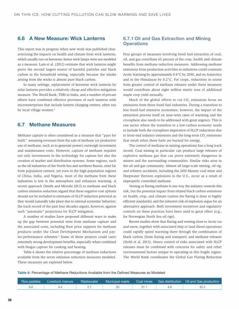
On thin ice: hOw cutting pOllutiOn can slOw warming and save lives
58
6.6 A New Measure: Wick Lanterns
This report was in progress when new work was published char-acterizing the impacts on health and climate from wick lanterns, which usually run on kerosene; hence wick lamps were not modeled as a measure. Lam et al. (2012) estimate that wick lanterns might prove the second largest source of harmful particles and black carbon in the household setting, especially because the smoke arising from the wicks is almost pure black carbon.
In many settings, replacement of kerosene wick lanterns by solar lanterns provides a relatively cheap and effective mitigation measure. The World Bank, TERI in India, and a number of private efforts have combined effective provision of such lanterns with microenterprises that include lantern charging centers, often run by local village women.5
6.7 Methane Measures
Methane capture is often considered as a measure that “pays for itself,” assuming revenues from the sale of methane (or productive use of methane, such as to generate power) outweigh investment and maintenance costs. However, capture of methane requires not only investments in the technology for capture but also the creation of market and distribution systems. Some regions, such as the oil industries of the North Sea and northern Russia, exist far from population centers; yet even in the high-population regions of China, India, and Nigeria, most of the methane from these industries is lost to the atmosphere and enhances warming. A recent approach (Smith and Mizrahi 2013) to methane and black carbon emission reduction argued that these negative-cost options should not be included in estimates of SLCP reduction potential as they would naturally take place due to rational economic behavior; the track record of the past four decades argues, however, against such “automatic” projections for SLCP mitigation.
A number of studies have proposed different ways to make up the gap between potential wins from methane capture and the associated costs, including floor price supports for methane products under the Clean Development Mechanism and pay-for-performance schemes.6 Some of these projects could carry extremely strong development benefits, especially when combined with biogas capture for cooking and heating.
Table 6 shows the relative percentage of methane reductions available from the seven emission reduction measures modeled. These measures are explored below.
6.7.1 Oil and Gas Extraction and Mining Operations
Four groups of measures involving fossil fuel extraction of coal, oil, and gas contribute 65 percent of the crop, health and climate benefits from methane reduction measures. Addressing methane emissions from production activities in industries could constrain Arctic warming by approximately 0.4°C by 2050, and on Antarctica and in the Himalayas by 0.2°C. For crops, reductions in ozone from greater control of methane releases under these measures would contribute about eight million metric tons of additional staple crop yield annually.
Much of the global efforts to cut CO2 emissions focus on
emissions from these fossil fuel industries. During a transition to less fossil-fuel intensive economies, however, the impact of the extraction process itself on near-term rates of warming and the cryosphere also needs to be addressed with great urgency. This is one sector where the transition to a low-carbon economy needs to include both the cryosphere imperative of SLCP reductions due to front-end industry emissions and the long-term CO2 emissions that result when these fuels are burned for energy.
The control of methane in mining operations has a long track record. Coal mining in particular can produce large releases of explosive methane gas that can prove extremely dangerous to miners and the surrounding communities. Similar risks arise in the oil and gas community. Almost all large-scale mining, oil rig, and refinery accidents, including the 2010 Massey coal mine and Deepwater Horizon explosions in the U.S., occur as a result of improperly controlled methane.
Venting or flaring methane is one way the industry controls this risk, but the potential impact from related black carbon emissions on health, crop, and climate (unless the flaring is done to highly efficient standards) and the inherent risk of explosion argue for an alternative approach. Both investment incentives and regulatory controls on these practices have been used to great effect (e.g., for Norwegian North Sea oil rigs).
Recent studies show that flaring and venting close to Arctic ice and snow, together with associated ship or land diesel operations could rapidly speed warming there through the combination of black carbon (from flaring and transport) and methane releases (Stohl et al. 2013). Hence control of risks associated with SLCP releases must be combined with concerns for safety and other environmental factors unique to operating in this fragile region. The World Bank coordinates the Global Gas Flaring Reduction
Table 6:PercentageofMethaneReductionsAvailablefromtheDefinedMeasuresasModeled
Rice paddies Livestock manure Wastewater Municipal waste Coal mines Gas distribution Oil and Gas production6.6 4.4 2.7 20 31.1 4.9 30.3
dIsCUssIon: ImPlICatIons for seCtoral aCtIons
59
initiative that is working with public and private entities to address issues of venting and flaring in the oil and gas industry.7
6.7.2 Wastewater and Landfills
Waste management measures, for wastewater treatment and municipal waste or landfills, provided about 23 percent of the methane-related climate, health, and crop benefits in each region and globally. Implementation of these two measures is almost cer-tain to bring additional benefits from the decrease in water-borne infectious diseases that comes with improved sanitation and water quality. Unfortunately, retrofitting of existing wastewater treat-ment plants to capture methane can prove expensive. However, the added cost in building these technologies into plant design from the beginning may prove much lower.
Capture of methane from existing landfills does provide a negative cost over time, but the high up-front investment costs can be a significant barrier to implementation. New landfills, on the other hand, may be built in a manner that avoids methane production entirely. There is some evidence that landfill owners have designed new sites in a manner that includes methane pro-duction and capture; they still run the risk, however, of generating fugitive emissions.8 Flaring of methane emissions leads to the production of black carbon, substituting one pollutant for another and creating higher levels of particle pollution around landfill sites.
6.7.3 Agriculture
Improvements to agriculture, whether from the modeled measures for rice paddies or livestock (or from controlling open burning) can bring additional benefits in terms of improved food security and crop yields, providing 11 percent of the total global and regional methane reduction measure benefits.
A number of programs already seek to address methane emis-sions from agricultural activities. Methane from livestock manure is one of the fastest-growing sources of emissions, due to increased demand for meat across the globe. Current methane emissions from this source are estimated at around 20 percent of the global total. The modeling shows a far lower emission reduction poten-tial from livestock methane capture, about four percent, simply because the most proven technologies apply only to the largest livestock operations. However, commercially viable “methane cooker” biogas technologies exist at much smaller scales, includ-ing at the household level. They can effectively address cookstove emissions at the same time by employing biogas for cooking rather than biomass. This combination makes household scale manure management one of the more promising SLCP mitigation methods.
Emissions from flooded or wet-method rice paddies contribute a far larger proportion of estimated global anthropogenic methane than current potential reductions: fully 20 percent of anthropogenic
methane emissions come from rice agriculture. As with open burning, however, proven alternative rice agriculture methods exist that can maintain yields while decreasing reliance on water resources and fertilizer by using an integrated approach to properly time both fertilizer application and irrigation. For example, many rice varieties in wide use today do not require the constant 3–4 months of flooding currently employed. Although not included as an emission reduction measure in this report, the potential also exists for improved varieties of rice that can produce a much larger crop per paddy area and thus decrease the area of flooded fields.
In addition, use of compounds such as ammonium sulphate, which enhance activity of microbial groups that do not produce methane, can cut methane emissions under certain conditions. China has proven a leader in studying methane emissions from rice and providing alternative rice production methods. Recent studies indicate substantial emission reduction potential should other countries adopt these methods more widely.9
6.8 Operational Implications for Development Financing
This report models the impacts of methane and black carbon emissions on the cryosphere regions of the world, and assesses the technical potential of pre-identified mitigation measures (based on a prior UNEP/WMO Assessment) to deliver climate and develop-ment benefits. The report does not explore how to operationalize these measures, specifically the costs, benefits, challenges, and trade-offs associated with their implementation in various regions or countries; nor does it assess local implementation capacity and sustainability. Efforts to more widely implement these measures in the development context would need to be preceded by an options analysis that would evaluate the measures against these and other country-specific criteria and an assessment of financ-ing models that could make these mitigation measures a reality. In conducting such an evaluation, it would be helpful to look at existing experience with implementing programs in relevant sectors. The World Bank’s experience implementing cookstoves programs and the Global Gas Flaring Reduction initiative’s experience with venting and flaring in the oil and gas sector are two examples that could be useful.
When assessing the benefits of intervention programs, it is less common to focus on assessing their multiple benefits (e.g., for the cryosphere, health, and agriculture as in this case). Assess-ing investment programs through a comprehensive cost-benefit framework might provide a different prioritization of intervention options than conventional cost-benefit analysis. Methodologies and tools would need to be developed to allow such analysis and support decision makers with robust (economic) options analysis.

On thin ice: hOw cutting pOllutiOn can slOw warming and save lives
60
The findings of this report highlight the imperative to explore sectoral interventions that can benefit the cryosphere and devel-opment given the rapidly closing window to slow cryosphere changes. Enhanced outreach coupled with further regional or country-specific analytical work and stakeholder engagement
could help inform operations about how to help preserve the cryosphere and decrease the risks associated with cryosphere loss while, at the same time, delivering other important devel-opment benefits.
Endnotes1 With the important addition of energy efficiency measures and new technologies. For example, substitution of an electric car for an older diesel vehicle would also cut short-lived pollutant emissions.2 See examples at the Global Alliance for Clean Cookstoves: www.cleancookstoves.org.3 See www-ramanathan.ucsd.edu/files/PilotPhase-Final-June%2013.ppt.4 See www.nordic-ecolabel.org/.5 www.lightingafrica.org6 See the World Bank Report of the Methane Finance Study Group (http://documents.worldbank.org/curated/en/2013/04/18114933/methane-finance-study-group-report-using-pay-for-performance-mechanisms-finance-methane-abatement) and various publications of the Methane Blue Ribbon Panel (www.globalmethanefund.org).7 www.ggfr.org.8 Sierra Club Report on Landfill Gas-to-Energy (January 2010). See www.sierraclub.org/policy/conservation/landfill-gas-report.pdf.9 Nature News (2009).

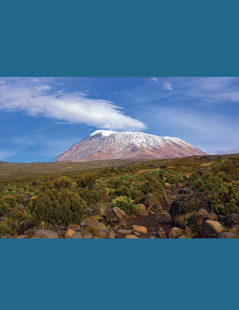
63
Abdul-Razzak and Ghan. 2000. A Parameterization of Aerosol Activation 2: Multiple Aerosol Types. J. Geophys. Res., vol. 105, pp. 6837–6844.
Amann, M., I. Bertok, J. Borken-Kleefeld, J. Cofala, C. Heyes, L. Höglund-Isaksson, Z. Klimont, B. Nguyen, M. Posch, P. Rafaj, R. Sandler, W. Schöpp, F. Wagner, and W. Winiwarter. 2011. Cost-effective Control of Air Quality and Greenhouse Gases in Europe: Modeling and Policy Applications. Environ. Model.
Softw. 26, 1489–1501.Anenberg, S. C., L. W. Horowitz, D. Q. Tong, and J. J. West. 2010.
An Estimate of the Global Burden of Anthropogenic Ozone and Fine Particulate Matter on Premature Human Mortality using Atmospheric Modeling. Environ. Health Perspect. 118, 1189–1195.
Arctic Council Task Force on Short Lived Climate Forcers. 2013. Recommendations to Reduce Black Carbon and Methane Emissions to Slow Arctic Climate Change.
Arctic Monitoring and Assessment Program. 2013. AMAP Arctic Ocean Acidification Assessment.
Arctic Monitoring and Assessment Program. 2011. Arctic Monitoring and Assessment Program. 2009. Black Carbon
in the Arctic.Arctic Monitoring and Assessment Program. 2009. Update on
Selected Climate Issues of Concern (Observations, Short-lived Climate Forcers, Arctic Carbon Cycle, Predictive Capability).
Arenas, López, and Ramírez Cadena. 2010. Glaciares, Nieves y Hielos de América. Latina Cambio – UNESCO.
Armstrong, R.L. 2010. The Glaciers of the Hindu Kush-Himalayan Region. A Summary of the Science Regarding Glacier Melt/Retreat in the Himalayan, Hindu Kush, Karakoram, Pamir, and Tien Shan Mountain Ranges. Technical Paper. Kathmandu. ICIMOD and USAID. ISBN 978 92 9115 173 8.
Asian Development Outlook. July 2013. Pakistan: p.208.Bamber, J. 2012. Climate Change: Shrinking Glaciers Under Scru-
tiny. Nature 482, 482–483.Bamber, J. et al. 2009. Reassessment of the Potential Sea-Level
Rise from a Collapse of the West Antarctic Ice Sheet. Science V. 324 no. 5929 pp. 901–903.
Bamber, J.L. and W.P. Aspinal. 2013. “An Expert Judgment Assess-ment of Future Sea-level Rise from the Ice Sheets.” Nature
Climate Change. Published online January 6. DOI: 10.1038/NCLIMATE1778.
Bassis, J.N., and S. Jacobs. 2013. Diverse Calving Patterns Linked to Glacier Geometry. Nature Geoscience (2013) doi:10.1038/ngeo1887.
Bednarsek, N., G.A. Tarling, D.C.E. Bakker, S. Fielding, E.M. Jones, H.J. Venables, P. Ward, A. Kuzirian, Be Leze, R.A. Feely, and E.J. Murphy. 2012. Extensive Dissolution of Live Pteropods in the Southern Ocean. Nature Geoscience 5: 881–885.
Bisiaux, M.M., et al. (2012). Variability of Black Carbon Deposition to the East Antarctic Plateau, 1800–2000 AD. Atmos. Chem. Phys. 12: 3799–3808.
Bolch, T., A. Kulkarni, A. Kääb, C. Huggel, F. Paul, J.G. Cogley, H. Frey, J.S. Kargel, K. Fujita, M. Scheel, S. Bajracharya, and M. Stoffel. 2012. The State and Fate of Himalayan Glaciers. Science 336, 301.
Bond, T. C., S. J. Doherty, D. W. Fahey, P. M. Forster, T. Berntsen, B. J. DeAngelo, M. G. Flanner, S. Ghan, B. Kärcher, D. Koch, S. Kinne, Y. Kondo, P. K. Quinn, M. C. Sarofim, M. G. Schultz, M. Schulz, C. Venkataraman, H. Zhang, S. Zhang, N. Bel-louin, S. K. Guttikunda, P. K. Hopke, M. Z. Jacobson, J. W. Kaiser, Z. Klimont, U. Lohmann, J. P. Schwarz, D. Shindell, T. Storelvmo, S. G. Warren, and C. S. Zender. 2013. Bounding the Role of Black Carbon in the Climate System: A Scientific Assessment. Journal of Geophysical Research: Atmospheres, 10.1002/jgrd.50171).
Box, J.E., et al. 2012. Arctic Report Card: 2012 Update.Bury, J.T. et al. 2011. Glacier Recession and Human Vulnerability
in the Yanamarey Watershed of the Cordillera Blanca, Peru. Climate Change Volume 105, Issue 1–2, pp 179–206.
Buytaert et al. 2011. Renewable and Sustainable Energy Reviews 15 (2011) 3918–3933.
Chen, J.L., C.R. Wilson, D. Blakenship, and B.D. Tapley. 2009. “Accelerated Antarctic Ice Loss from Satellite Gravity Mea-surements.” Nature Geoscience, Volume 2. December. DOI: 10.1038/NGEO694
Cheng, G. and H. Jin. 2103. Permafrost and Groundwater on the Qinghai-Tibet Plateau and in Northeast China. Hydrogeology Journal 21(1):5–23.
Christensen, M. and G. Stephens. 2011. Microphysical and Mac-rophysical Responses of Marine Stratocumulus Polluted by Underlying Ships: Evidence of Cloud Deepening. 2011. J. Geophys. Res. 116, D03201, doi:10.1029/2010JD014638.
CONDESAN. 2012. Sustainable Mountain Development in the Andes.
Bibliography
On thin ice: hOw cutting pOllutiOn can slOw warming and save lives
64
O’Connor et al. 2013. Evaluation of the New UKCA Climate-Composition Model – Part 2: The Troposphere. Geosci. Model Dev. Discuss., 6, 1743–1857.
Cullen, N.J. et al. 2002. A Century of Ice Retreat on Kilimanjaro: The Mapping Reloaded. Cryosphere 7(2): 419–431.
Delucchi, M. A. , and M. Z. Jacobson. 2011. Providing all Global Energy with Wind, Water, and Solar Power, Part II: Reliability, System and Transmission Costs, and Policies. Energy Policy 39, 1170–1190.
Dentener, F., S. Kinne, T. Bond, O. Boucher, J. Cofala, S. Generoso, P. Ginoux, S. Gong, J. J. Hoelzemann, A. Ito, L. Marelli, J. E. Penner, J.-P. Putaud, C. Textor, M. Schulz, G. R. van der Werf, and J. Wilson. 2006. Emissions of Primary Aerosol and Precursor Gases in the Years 2000 and 1750, Prescribed Data-sets for AeroCom. Atmos. Chem. Phys. 6, 2703–2763.
Dyurgerov, Mark B. and Mark F. Meier. 2004. Glaciers and the Changing Earth System: A 2004 Snapshot. INSTAAR, University of Colorado at Boulder.
Environmental Protection Agency. 2012. Report to Congress on Black Carbon, p.175.
European Environment Agency. 2013. The Impact of International Shipping on European Air Quality and Climate Forcing. EEA Technical Report No. 4/2013.
Feichter, J. E. Kjellstrom, H. Rodhe, F. Dentener, J. Lelieveld, and G. Roelofs. 1996. Simulation of the Tropospheric Sulfur Cycle in a Global Climate Model. Atmos. Env. 30, 1693–1707.
Flannigan, M. D., M. A. Krawchuk, W. J. de Groot, B. M. Wotton, and L. M. Gowman. 2009. Implications of Changing Climate for Global Wildland Fire. International Journal of Wildland
Fire 18:483-507.Flores, H. et al. 2012. Impact of Climate Change on Antarctic Krill.
Marine Ecology Progress Series 458: 1–19.Fujita,K, and T. Nuimura. 2011. Spatially Heterogeneous Wastage of
Himalayan Glaciers. Proc Natl Acad Sci USA 108(34):14011–14014.Gardner et al. 2013. “A Reconciled Estimate of Glacier Contributions
to Sea Level Rise: 2003 to 2009.” Science 340(6134): 852–857.Gauss, M., G. Myhre, I.S.A. Isaksen, V. Grewe, G. Pitari, O. Wild,
W.J. Collins, F.J. Dentener, K. Ellingsen, L.K. Gohar, D.A. Hauglustaine, D. Iachetti, F. Lamarque, E. Mancini, L.J. Mick-ley, M.J. Prather, J.A. Pyle, M.G. Sanderson, K.P. Shine, D.S. Stevenson, K. Sudo, S. Szopa, and G. Zeng. 2006. Radiative Forcing since Pre-industrial Times due to Ozone Change in the Troposphere and the Lower Stratosphere. Atmos. Chem. Phys., 6, 575–599, doi:10.5194/acp-6-575-2006.
Giri, C., and S. Shrestha. 2000. Forest Fire Mapping in Huay Kha Khaeng Wildlife Sanctuary, Thailand. International Journal
of Remote Sensing 21:2023–2030.Glasser et al. 2011. Global Sea-level Contribution from the Pata-
gonian Icefields since the Little Ice Age Maximum. Nature
Geoscience 4, 303–307.
Goelzer et al. 2013. Sensitivity of Greenland Ice Sheet Projections to Model Formulations.
Guenther, A., T. Karl, P. Harley, C. Wiedinmyer, P.I. Palmer, and C. Geron. 2006. Estimates of global terrestrial isoprene emissions using MEGAN (Model of Emissions of Gases and Aerosols from Nature), Atmos. Chem. Phys., 6, 3181–3210, doi:10.5194/acp-6-3181-2006.
Guenther, A., C. N. Hewitt, D. Erikson, R. Fall., C. Geron, T. Grae-del, P. Harley, L. Klinger, M. Lerdau, W. A. McKay, T. Pierce, B. Scoles, R. Seinbrecher, R. Tallamraju, J. Taylor, and P. Zim-merman. 1995. A Global Model of Natural Volatile Organic Compound Emissions. J. Geophys. Res. 100, 8873–8892.
Journal of Glaciology, Vol. 59, No. 216, 2013 doi:10.3189/2013JoG12J182 733.
Hagemann, S., K. Arpe, and E. Roeckner. 2006. Evaluation of the Hydrological Cycle in the ECHAM5 Model. J. Clim. 19, 3810–3827.
Hall, S., and S. Thatje. 2011. Temperature-driven Biogeography of the Deep-sea Family Lithodidae (Crustacea: Decapoda: Anomura) in the Southern Ocean. Polar Biology 34: 363-370.
Herzog et al. 2011. Climate Change and Biodiversity in the Tropical Andes, Inter-American Institute for Global Change Research.
Hess, P., and N. Mahowald. 2009. Interannual Variability in Hindcasts of Atmospheric Chemistry: The Role of Meteo-rology. Atmos. Chem. Phys., 9, 5261–5280, doi:10.5194/acp-9-5261-2009.
Hewitt et al. 2011. Design and Implementation of the Infrastructure of HadGEM3: The Next-generation Met Office Climate Model-ing System. Geosci. Model Dev., 4, 223–253.
Hillenbrand C.D., G. Kuhn, J.A. Smith, K. Gohl, A.G.C. Graham, R.D. Larter, J.P. Klages, R. Downey, S.G. Moreton, M. Forwick, and D.G. Vaughan. 2012. “Grounding-line Retreat of the West Antarctic Ice Sheet from Inner Pine Island Bay” Geology. Pub-lished online October 19. Doi: 10.1130/G33469.1.
Horowitz, L. W. , S. Walters, D. L. Mauzerall, L. K. Emmons, P. J. Rasch, C. Granier, X. X. Tie, J.-F. Lamarque, M. G. Schultz, G. S. Tyndall, J. J. Orlando, and G. P. Brasseur. 2003. A Global Simulation of Tropospheric Ozone and Related Tracers: Descrip-tion and Evaluation of MOZART, version 2. J. Geophys. Res. 108(D24), 4784, doi:10.1029/2002JD002853.
Hu, A., Y. Xu, C. Tebaldi, W.M. Washington, and V. Ramanathan. 2013. Mitigation of Short-lived Climate Pollutants Slows Sea-level Rise. Nature Climate Change doi:10.1038/nclimate1869.
IFFN-GFMC. 2011. UNISDR Global Wildland Fire Network Bulletin Issue No. 15: #1, July 31.
Immerzeel, W.W., L.P.H. van Beek, and M.F.P. Bierkens. 2010. Climate Change Will Affect the Asian Water Towers. Science 328(5984):1382–1385.
International Agency for Research on Cancer. 2012. IARC Mono-graphs on the Evaluation of Carcinogenic Risks to Humans.
dIsCUssIon: ImPlICatIons for seCtoral aCtIons
65
T. Ramsay, Z. Ross, H. Shin, and B. Tempalski. 2009. “Extended Follow-up and Spatial Analysis of the American Cancer Society Study Linking Particulate Air Pollution and Mortality.” Health Effects Institute research report.
Kvalevåg, M. M., and G. Myhre. 2007. Human Impact on Direct and Diffuse Solar Radiation during the Industrial Era. J. Clim. 20, 4874–4883.
Lam, N.L. et al. 2012. “Household Light Makes Global Heat: High Black Carbon Emissions From Kerosene Wick Lamps.” Environmental Science & Technology , 46, (24), 13531- 13538.
Lawrence, D.M. et al. 2008. “Accelerated Arctic Land Warming and Permafrost Degradation during Rapid Sea Ice Loss.” Geophysi-
cal Research Letters 35 (11): L11506.Lee, Y., and P. Adams. 2012. A Fast and Efficient Version of the
TwO-Moment Aerosol Sectional (TOMAS) Global Aerosol Micro-physics Model. Aerosol Science and Technology 46, 678–689 (2012); published online Epub (10.1080/02786826.2011.643259).
Lin, S. J., and R. B. Rood. 1996. Multidimensional Flux-form Semi-Lagrangian Transport Schemes. Mon. Weather Rev. 124, 2046–2070.
Liu, J., et al. 2013. The Two Main Mechanisms of Glacier Outburst Flood in Tibet, China. J. Mt. Sci. 10(2):239-248.
Mann et al. 2010. Description and Evaluation of GLOMAP-mode: A Modal Global Aerosol Microphysics Model for the UKCA Composition-Climate Model. Geosci. Model Dev., 3, 519-551, doi:10.5194/gmd-3-519-2010.
McNeil, B.J., and R.J. Matear. 2008. Southern Ocean Acidification: A Tipping Point at 450-ppm Atmospheric CO2. Proceedings of
the National Academy of Sciences 105: 18860-188864.Menon, S., J.E. Hansen, L. Nazarenko, and Y. Luo. 2002. “Climate
Effects of Black Carbon Aerosols in China and India.” Science 297 (5590): 2250–2253.
Mölg, Thomas et al. 2013. East African Glacier Loss and Climate Change. Environmental Development 6:1–6.
Mölg, Thomas et al. 2012. Limited Forcing of Glacier Loss through Land-cover Change on Kilimanjaro. Nature DOI: 10.1038/NCLIMATE1390.
Mölg, Thomas et al. 2010. “Glacier Loss on Kilimanjaro is an Exceptional Case.” Proceedings of the National Academy of Sciences of the United States of America 107(17): E68-E68.
Mölg, Thomas, Nicolas J. Cullen, Douglas R. Hardy, Michael Winkler, and Georg Kaser. 2009. Quantifying Climate Change in the Tropical Midtroposphere over East Africa from Glacier Shrinkage on Kilimanjaro. J. Climate, 22, 4162–4181.
Mulvaney, R., N.J. Abram, R.C.A. Hindmarsh, C. Arrowsmith, L. Fleet, J. Triest, L.C. Sime, O. Alemany, and S. Foord. 2012. “Recent Antarctic Peninsula Warming Relative to Holocene Climate and Ice-shelf History.” Nature 489:141-144. Doi:10.1038/nature11391.
National Snow and Ice Data Center. 2013. Arctic Ice News and Analysis. http://nsidc.org/arcticseaicenews/.
Vol. 105: DIESEL AND GASOLINE ENGINE EXHAUSTS AND SOME NITROARENES. Lyon, France: June 5–12.
International Energy Agency and Norden. 2012. “Nordic Energy Technology Perspectives.”
IPCC Working Group I Report. Sept. 27, 2013.
Isaksen, I. S. A., C. Granier, G. Myhre, T. K. Berntsen, S. B. Dalsøren, M. Gauss, Z. Klimont, R. Benestad, P. Bousquet, W. Collins, T. Cox, V. Eyring, D. Fowler, S. Fuzzi, P. Jockel, P. Laj, U. Lohm-ann, M. Maione, P. Monks, A. S. H. Prevot, F. R. Raes, A. , B. Rognerud, M. Schulz, D. Shindell, D. S. Stevenson, T. Storelvmo, W.-C. Wang, M. van Weele, M. Wild, and D. Wuebbles. 2009. Atmospheric Composition Change: Climate–Chemistry Interac-tions. Atmos. Env. 43, 5138–5192.
Jazcilevich, A.D., A. G. Reynoso, M. Grutter, J. Delgado, U. D. Ayala, M. S. Lastra, M. Zuk, R. G. Oropeza, J. Lents, and N. Davis. 2011. An Evaluation of the Hybrid Car Technology for the Mexico Mega City. J. Power Sources 196, 5704–5718.
Jerrett, M., R. T. Burnett, C. A. I. Pope, K. Ito, G. Thurston, D. Krewski, Y. Shi, E. Calle, and M. Thun. 2009. Long-Term Ozone Exposure and Mortality. New Engl. J. Med. 360, 1085–1095.
Joughin, I., and R.B. Alley. 2011. “Stability of the West Antarctic Ice Sheet in a Warming World.” Nature Geoscience. 4:506-513. Doi:10.1038/ngeo1194.
Joughin, I., B.E. Smith, and D.M. Holland. 2010. “Sensitivity of 21st Century Sea Level to Ocean-induced Thinning of Pine Island Glacier, Antarctica.” Geophysical Research Letters. 37: L20502.
Kaab A, E. Berthier, C. Nuth, J. Gardelle, and Y Arnaud. 2012. Contrasting Patterns of Early Twenty-First-Century Glacier Mass Change in the Himalayas. Nature 488: 495–498.
Kang, S. et al. 2010. Review of Climate and Cryospheric Change in the Tibetan Plateau. Environ Res Lett 5(1):015101, doi:10.1088/1748-9326/5/1/015101.
Kaser et al. 2004. Glacier Retreat on Kilimanjaro as Evidence of Climate Change. Int. J. Climatol. 24: 329–339.
Kinne, S., M. Schulz, C. Textor, S. Guibert, Y. Balkanski, S.E. Bauer, T. Berntsen, T.F. Berglen, O. Boucher, M. Chin, W. Collins, F. Dentener, T. Diehl, R. Easter, J. Feichter, D. Fillmore, S. Ghan, P. Ginoux, S. Gong, A. Grini, J. Hendricks, M. Herzog, L. Horowitz, I. Isaksen, T. Iversen, A. Kirkev°ag, S. Kloster, D. Koch, J.E. Kristjansson, M. Krol, A. Lauer, J.F. Lamarque, G. Lesins, X. Liu, U. Lohmann, V. Montanaro, G. Myhre, J. Penner, G. Pitari, S. Reddy, O. Seland, P. Stier, T. Takemura, and X. Tie. 2006. An AeroCom Initial Assessment – Optical Properties in Aerosol Component Modules of Global Models. Atmos. Chem. Phys., 6, 1815–1834, doi:10.5194/acp-6-1815-2006.
Kohler and Maselli. 2009. Mountains and Climate Change: From Understanding to Action. Geographica Bernensia.
Krewski, D., M. Jerrett, R. Burnett, R. Ma, E. Hughes, Y. Shi, M. C. Turner, P. C. A. 3rd, G. Thurston, E. Calle, M. Thun, B. Becker-man, P. DeLuca, N. Finkelstein, K. Ito, D. Moore, K. Newbold,
On thin ice: hOw cutting pOllutiOn can slOw warming and save lives
66
Forcing since Pre-industrial Times due to Ozone Change in the Troposphere and the Lower Stratosphere. Atmos. Chem. Phys., 6, 575–599, doi:10.5194/acp-6-575-2006.
Prather, M.J. 1986. Numerical Advection by Conservation of Second-order Moments. J. Geophys. Res. 91, 6671–6681.
Pritchard, H.D., S.R.M. Ligtenberg, H.A. Fricker, D.G. Vaughan, M.R. van den Broeke, and L. Padman. 2012. “Antarctic Ice-sheet Loss driven by Basal Melting of Ice Shelves.” Nature.
484: 502-505. Doi:10.1038/nature10968.Quaas, J., O. Boucher, N. Bellouin, and S. Kinne. 2008. Satellite-
based Estimate of the Direct and Indirect Aerosol Climate Forc-ing. J. Geophys. Res. 113, D05204, doi:10.1029/2007JD008962.
Rabatel, A. et al. 2013. Current State of Glaciers in the Tropical Andes: a Multi-century Perspective on Glacier Evolution and Climate Change. The Cryosphere, 7, 81–102.
Ramankutty, N., A.T. Evan, C. Monfreda, and J.A. Foley. 2008. “Farming the Planet: 1. Geographic Distribution of Global Agricultural Lands in the Year 2000.” Global Biogeochemical Cycles, Vol. 22, GB1003, doi:10.1029/2007GB002952.
Rayner, N. A., D. E. Parker, E. B. Horton, C. K. Folland, L. V. Alexander, D. P. Rowell, E. C. Kent, and A. Kaplan. 2003. Global Analyses of Sea-Surface Temperature, Sea Ice, and Night Marine Air Temperature since the Late Nineteenth Century. J. Geophys. Res. 108, doi 10.1029/2002JD002670.
República de Argentina. 2007. Annual Report to UNFCCC. Rignot, E., I. Velicogna, M.R. van den Broeke, A. Monaghan, and
J.T.M. Lenaerts. 2011. “Acceleration of the Contribution of the Greenland and Antarctic Ice Sheets to Sea-level Rise.” Geophysi-
cal Research Letters. 38: L05503. Doi:10.1029/2011GL046583.
Rignot E., J.L. Bamber, M.R. van den Broeke, C. Davis, Y. Li, W.J. van de Berg, and E. van Meijgaard. 2008. “Recent Antarctic Ice Mass Loss from Radar Interferometry and Regional Climate Modeling.” Nature Geoscience 1: 106–110. doi:10.1038/ngeo102.
Riihelä et al. 2013. Observed Changes in the Albedo of the Arctic Sea-ice Zone for the Period 1982 to 2009. Nature Climate Change doi:10.1038/NCLIMATE1963.
Roeckner, E., R. Brokopf, M. Esch, M. Giorgetta, S. Hagemann, L. Kornblueh, E. Manzini, U. Schlese, and U. Schulzweida. 2006. Sensitivity of Simulated Climate to Horizontal and Vertical Resolu-tion in the ECHAM5 Atmosphere Model. J. Clim. 19, 3771–3791.
Rowley, R.J. et al. 2007. Risk of Rising Sea Level to Population and Land Area. EOS 88(9):105–107.
Sallenger, A.H. et al. 2012. Hotspot of accelerated sea-level rise on the Atlantic coast of North America. Nature Climate Change 2, 884–888.
Shadwick, E.W. et al. 2013. Vulnerability of Polar Oceans to Anthropogenic Acidification: Comparison of Arctic and Antarctic Seasonal Cycles. Scientific Reports 3: doi 10.1038/srep02339.
Nature News. 2009. doi:10.1038/news.2009.833.O’Donnell, Ryan, Nicholas Lewis, Steve McIntyre, and Jeff Con-
don. 2011. Improved Methods for PCA-based Reconstructions: Case Study using the Steig et al. (2009) Antarctic Temperature Reconstruction. J. Climate, 24, 2099–2115. doi: http://dx.doi.org/10.1175/2010JCLI3656.1.
Olivier, J.G.J. and J. J. M. Berdowski, in The Climate System, J. Berdowski, R. Guicherit, and B. J. Heij, eds. 2001. A.A. Balkema Publishers/Swets & Zeitlinger Publishers, Lisse,The Netherlands, pp. 33–78.
Parkinson, C.L., and D.J. Cavalieri. 2012. Antarctic Sea Ice Variability and Trends: 1979–010. The Cryosphere Discussions. 6:931-956.
Pausata, F.S.R., L. Pozzoli, R. Van Dingenen, E. Vignati, F. Cavalli, and F.J. Dentener. 2013. Impacts of Changes in North Atlantic Atmospheric Circulation on Particulate Matter and Human Health in Europe. DOI: 10.1002/grl.50720, GRL 2013.
Pausata, F.S.R., L. Pozzoli, E. Vignati, and F.J. Dentener. 2012. North Atlantic Oscillation and Tropospheric Ozone Variability in Europe: Model Analysis and Measurements Intercom-parison. Atmos. Chem. Phys., 12, 6357–6376, doi:10.5194/acp-12-6357-2012.
Penner, J. E., J. Quaas, T. Storelvmo, T. Takemura, O. Boucher, H. Guo, A. Kirkevag, J. E. Kristjansson, and O. Seland. 2006. Model Intercomparison of Indirect Aerosol Effects. Atmos.
Chem. Phys. 6, 3391–3405.Peterson, D. et al. 2010. Effects of Lightning and other Meteoro-
logical Factors on Fire Activity in the North American Boreal Forest: Implications for Fire Weather Forecasting. Atmos. Chem. Phys., 10, 6873–6888.
Pollard, David, and Robert M. DeConto. 2009. Modeling West Antarctic Ice Sheet Growth and Collapse through the Past Five Million Years. Nature 458: 329–332.
Pozzoli, L., G. Janssens-Maenhout, T. Diehl, I. Bey, M.G. Schultz, J. Feichter, E. Vignati, E., and F. Dentener. 2011. Re-analysis of Tropospheric Sulfate Aerosol and Ozone for the Period 1980–2005 using the Aerosol-Chemistry-Climate Model ECHAM5-HAMMOZ. Atmos. Chem. Phys., 11, 9563-9594, doi:10.5194/acp-11-9563-2011.
Pozzoli, L., I. Bey, S. Rast, M. G. Schultz, P. Stier, and J. Feichter. 2008a. Trace Gas and Aerosol Interactions in the Fully Coupled Model of Aerosol-Chemistry-Climate ECHAM5-HAMMOZ: 1. Model Description and Insights from the Spring 2001 TRACE-P Experiment. J. Geophys. Res. 113, D07308.
Pozzoli, L., I. Bey, S. Rast, M. G. Schultz, P. Stier, and J. Feichter. 2008b. Trace Gas and Aerosol Interactions in the Fully Coupled Model of Aerosol-Chemistry-Climate ECHAM5-HAMMOZ: 2. Impact of Heterogeneous Chemistry on the Global Aerosol Distributions. J. Geophys. Res. 113, D07309.
Prather, M.J., J.A. Pyle, M.G. Sanderson, K.P. Shine, D.S. Ste-venson, K. Sudo, S. Szopa, and G. Zeng. 2006. Radiative
dIsCUssIon: ImPlICatIons for seCtoral aCtIons
67
Steig, E.J. 2012. “Brief but Warm Antarctic Summer.” Nature.
489:39–41.Steig, E.J., and A.J. Orsi. 2013. “Climate Change: The Heat is on in
Antarctica.” Nature Geoscience. 6:87-88. doi:10.1038/ngeo1717.Steig, E.J., D.P. Schneider, S.D. Rutherford, M.E. Mann, J.C. Comiso,
and D.T. Shindell. 2009. “Warming of the Antarctic Ice-sheet Surface since the 1957 International Geophysical Year.” Nature
457:459-766. Doi:10.1038/nature07669.Stern et al. 2011. Temperature and Malaria Trends in Highland
East Africa. PLoS ONE 6(9): e24524.Stern. 2006. The Economics of Climate Change: The Stern Review.
Cambridge University Press.Stevenson, D., F. Dentener, M. Schultz, K. Ellingsen, T. van Noije, O.
Wild, G. Zeng, M. Amann, C. Atherton, N. Bell, D. Bergmann, I. Bey, T. Butler, J. Cofala, W. Collins, R. Derwent, R., Doherty, J. Drevet, H. Eskes, A. Fiore, M. Gauss, D. Hauglustaine, L. Horowitz, I. Isaksen, M. Krol, J. Lamarque, M. Lawrence, V. Montanaro, J. Muller, G. Pitari, M. Prather, J. Pyle, S. Rast, J. Rodriguez, M. Sanderson, N. Savage, D. Shindell, S. Strahan, K. Sudo, and S. Szopa. 2006. Multimodel Ensemble Simula-tions of Present-day and Near-future Tropospheric Ozone. J. Geophys. Res.-Atmos., 111, D08301, doi:10.1029/2005JD006338.
Stier, P., J., H. Seinfeld, S. Kinne, and O. Boucher. 2007. Aerosol Absorption and Radiative Forcing. Atmos. Chem. Phys., 7, 5237–5261, doi:10.5194/acp-7-5237-2007.
Stier, P., J. Feichter, S. Kinne, S. Kloster, E. Vignati, J. Wilson, L. Ganzeveld, I. Tegen, M. Werner, Y. Balkanski, M. Schulz, O. Boucher, A. Minikin, and A. Petzold. 2005. The Aerosol-Climate Model ECHAM5-HAM. Atmos. Chem. Phys. 5, 1125–1156.
Stroeve, J., J. Box, Z. Wang, A. Barrett, and C. Schaaf. 2013. Re-evaluation of MODIS Greenland Albedo Accuracy and Trends. Remote Sensing of the Environment, in revision.
Stohl, Andreas et al. 2013. Why Models Struggle to Capture Arctic Haze: The Underestimated Role of Gas Flaring and Domestic Combustion Emissions. Atmos. Chem. Phys. Discuss. 13, 9567–9613.
Stone, E.J. et al. 2010. Investigating the Sensitivity of Numeri-cal Model Simulations of the Modern State of the Greenland Ice-sheet and its Future Response to Climate Change. The Cryosphere, 4, 397–417.
Taylor, R.G. et al. 2009. Recent Glacial Recession and its Impact on Alpine Riverflow in the Rwenzori Mountains of Uganda. Journal of African Earth Sciences 55(3–4), 205–213.
Taylor, R.G. et al. 2006. Recent Glacial Recession in the Rwenzori Mountains of East Africa due to Rising Air Temperature. Geo-phys. Res. Lett., 33, L10402.
Thompson, L.G. et al. 2009. Glacier Loss on Kilimanjaro Continues Unabated. PNAS 106(47):19770–75.
Turner, G. and H. Annamalai. 2012. Climate Change and the South Asian Summer Monsoon. Nature Climate Change 2, 587–595.
Shakhova, N. et al. 2010. Geochemical and Geophysical Evidence of Methane Release over the East Siberian Arctic Shelf. Journal of Geophysical Research 115, C08007.
Shakhova, N. et al. 2010. Extensive Methane Venting to the Atmosphere from Sediments of the East Siberian Arctic Shelf. Science 327, 1246-1250.
Shakhova, N.E., V.A. Alekseev, and I.P. Semiletov. 2010. Doklady
Earth Sci. 430, 190–193.
Shakti Sustainable Energy Foundation. 2012. Brick Kilns Performance Assessment: A Road for Cleaner Brick Production in India.
Shindell, D. T., O. Pechony, A. Voulgarakis, G. Faluvegi, L. Nazarenko, J. F. Lamarque, K. Bowman, G. Milly, B. Kovari, R. Ruedy, and G. A. Schmidt. 2013a. Interactive Ozone and Methane Chemistry in GISS-E2 Historical and Future Climate Simulations. Atmos. Chem. Phys. 13, 2653-2689; 10.5194/acp-13-265.3-2013).
Shindell, D. T. , J. F. Lamarque, M. Schulz, M. Flanner, C. Jiao, M. Chin, P. J. Young, Y. H. Lee, L. Rotstayn, N. Mahowald, G. Milly, G. Faluvegi, Y. Balkanski, W. J. Collins, A. J. Conley, S. Dalsoren, R. Easter, S. Ghan, L. Horowitz, X. Liu, G. Myhre, T. Nagashima, V. Naik, S. T. Rumbold, R. Skeie, K. Sudo, S. Szopa, T. Takemura, A. Voulgarakis, J. H. Yoon, and F. Lo. 2013b. Radiative Forcing in the ACCMIP Historical and Future Climate Simulations. Atmos. Chem. Phys. 13, 2939–2974; 10.5194/acp-13-2939-2013).
Shindell, D., J. C. I. Kuylenstierna, E. Vignati, R. Van Dingenen, M. Amann, Z. Klimont, S. C. Anenberg, N. Z. Muller, G. Janssens-Maenhout, F. Raes, J. Schwartz, G. Faluvegi, L. Pozzoli, K. Kupiainen, L. Hoglund-Isaksson, L. Emberson, D. Streets, V. Ramanathan, K. Hicks, N. T. K. Oanh, G. Milly, M. Williams, V. Demkine, and D. Fowler. 2012. Simultaneously Mitigating Near-Term Climate Change and Improving Human Health and Food Security. Science 335, 183–189.
Shrestha, U.B., S. Gautam, and K.S. Bawa. 2012. Widespread Climate Change in the Himalayas and Associated Changes in Local Ecosystems. PLoS One 7(5): e36741. Doi:10.1371/journal.pone.0036741.
Smith, C.R., L.J. Grange, D.L. Honig, L. Naudts, L. Guidi, and E. Domack. 2012. A Large Population of King Crabs in Palmer Deep on the West Antarctic Peninsula Shelf and Potential Invasive Impacts. Proceedings of the Royal Society B 279: 1017–1026.
Smith, Steven J., and Andrew Mizrahi. 2013. “Near-Term Climate Mitigation by Short-Lived Forcers.” PNAS, August 12: DOI 10.1073/pnas.1308470110.
Snow, Water, Ice, and Permafrost in the Arctic (SWIPA): www.amap.no.
Spada, G. , J. L. Bamber, and R. T. W. L. Hurkmans. 2013. The Gravitationally Consistent Sea-level Fingerprint of Future Terrestrial Ice Loss. Geophysical Research Letters, 2013; DOI: 10.1029/2012GL053000.
On thin ice: hOw cutting pOllutiOn can slOw warming and save lives
68
Working Group I Contribution to the IPCC Fifth Assessment Report. 2013. Climate Change 2013: The Physical Science Basis. Sum-mary for Policymakers, 27 September, p. SPM-20.
World Health Organization. 2011. EM-DAT, The International Disaster Database.
World Bank. 2013. China: Accelerating Household Access to Clean
Cooking and Heating.World Bank. 2011. Household Cookstoves, Environment, Health,
and Climate Change: A New Look at an Old Problem.Wu, Q., and T. Zhang. 2008. Recent Permafrost Warming on
the Qinghai-Tibetan Plateau, J. Geophys. Res., 113, D13108, doi:10.1029/2007JD009539.
Xu, C. et al. 2006. Climate Change and Hydrologic Process Response in the Tarim River Basin over the Past 50 Years. Chinese Sci-ence Bulletin 51(1): 25–26.
Xu, J., A. Shrestha, and M. Eriksson. 2009. Climate Change and its Impacts on Glaciers and Water Resource Management in the Himalayan Region. Assessment of Snow, Glacier and Water Resources in Asia. International Hydrological Programme of UNESCO and Hydrology and Water Resources Programme of WMO.
Yao, T. et al. 2012. Different Glacier Status with Atmospheric Circulations in Tibetan Plateau and Surroundings. Nat Clim
Chang 2(9):663–667.Young, J. and S. Hastenwrath. 1987. “Glaciers of the Middle East
and Africa.” U.S. Geological Professional Survey. U.S. Depart-ment of the Interior. pp. G61, G58, G59 G62.
Zhang, Q. et al. 2009. Variability and Stability of Water Resource in the Arid Regions of China: A Case study of the Tarim River Basin. Frontiers of Earth Science in China 3(4): 381–388.
Zimov, S. et al. 2006. Climate Change, Permafrost, and the Global Carbon Budget.” Science 312 (5780): 1612–3. doi:10.1126/science.1128908.
UNEP-GRID. September 2012. Measuring Glacier Change in the Himalayas. GEAS Thematic Focus.
UNEP Global Environmental Alert Service. 2012. Africa Without Glaciers.
United Nations Environment Programme. 2013. Africa Without Ice and Snow. Environmental Development 5:145+155.
United Nations Environment Programme. 2011. “Near-term Climate Protection and Clean Air Benefits: Actions for Controlling Short-Lived Climate Forcers.”
United Nations Environment Programme and World Meteorological Organization. 2011. “Integrated Assessment of Black Carbon and Tropospheric Ozone.”
Van Dingenen, R., F. J. Dentener, F. Raes, M. C. Krol, L. Emberson, and J. Cofala. 2009. The Global Impact of Ozone on Agricultural Crop Yields under Current and Future Air Quality Legislation. Atmos. Env. 43, 604–618.
Vaughan, D.G. et al. 2003. “Recent Rapid Regional Climate Warm-ing on the Antarctic Peninsula.” Climatic Change 60:243–274.
Velicogna, I. 2009. “Increasing Rates of Ice Mass Loss from the Green-land and Antarctic Ice Sheets Revealed by GRACE.” Geophysi-
cal Research Letters. 36, L19503, doi:10.1029/2009GL040222.Vergara et. al. 2007. Economic Impacts of Rapid Glacier Retreat in
the Andes. Eos Trans. AGU, 88(25), doi:10.1029/2007EO250001.Vignati, E., J. Wilson, and P. Stier. 2004. M7: An Efficient Size-
resolved Aerosol Microphysics Module for Large-scale Aerosol Transport Models. J. Geophys. Res. 109, D22202.
Whiteman, G. et al. 2013. Nature 499, 401–403 (25 July 2013) doi:10.1038/499401a.
Willis, M.J., A.K. Melkonian, M.E. Pritchard, and A. Rivera. 2012. Ice Loss from the Southern Patagonian Ice Field, South America, etween 2000 and 2012. Geophys. Res. Lett., 39.
Witze, Alexandra. 2008. Polar Creatures Squeaked Through Last Ice Age. Nature News 18 February 2008. Accessed 15 March 2013 from http://www.nature.com/news/2008/080218/full/news.2008.606.html.

dIsCUssIon: ImPlICatIons for seCtoral aCtIons
69

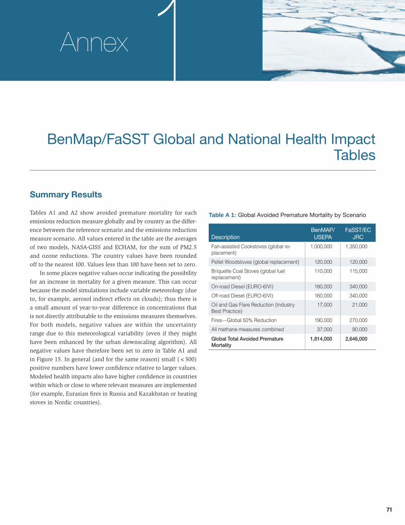
71
BenMap/FaSST Global and National Health Impact Tables
Summary Results
Tables A1 and A2 show avoided premature mortality for each emissions reduction measure globally and by country as the differ-ence between the reference scenario and the emissions reduction measure scenario. All values entered in the table are the averages of two models, NASA-GISS and ECHAM, for the sum of PM2.5 and ozone reductions. The country values have been rounded off to the nearest 100. Values less than 100 have been set to zero.
In some places negative values occur indicating the possibility for an increase in mortality for a given measure. This can occur because the model simulations include variable meteorology (due to, for example, aerosol indirect effects on clouds); thus there is a small amount of year-to-year difference in concentrations that is not directly attributable to the emissions measures themselves. For both models, negative values are within the uncertainty range due to this meteorological variability (even if they might have been enhanced by the urban downscaling algorithm). All negative values have therefore been set to zero in Table A1 and in Figure 15. In general (and for the same reason) small (<500) positive numbers have lower confidence relative to larger values. Modeled health impacts also have higher confidence in countries within which or close to where relevant measures are implemented (for example, Eurasian fires in Russia and Kazakhstan or heating stoves in Nordic countries).
Annex 1Table A 1: Global Avoided Premature Mortality by Scenario
DescriptionBenMAP/USEPA
FaSST/EC JRC
fan-assisted Cookstoves (global re-placement)
1,000,000 1,350,000
Pellet Woodstoves (global replacement) 120,000 120,000Briquette Coal stoves (global fuel replacement)
110,000 115,000
On-road Diesel (EURO-6/VI) 180,000 340,000Off-road Diesel (EURO-6/VI) 160,000 340,000oil and Gas flare reduction (Industry Best Practice)
17,000 21,000
Fires—Global 50% Reduction 190,000 270,000all methane measures combined 37,000 90,000Global Total Avoided Premature Mortality
1,814,000 2,646,000
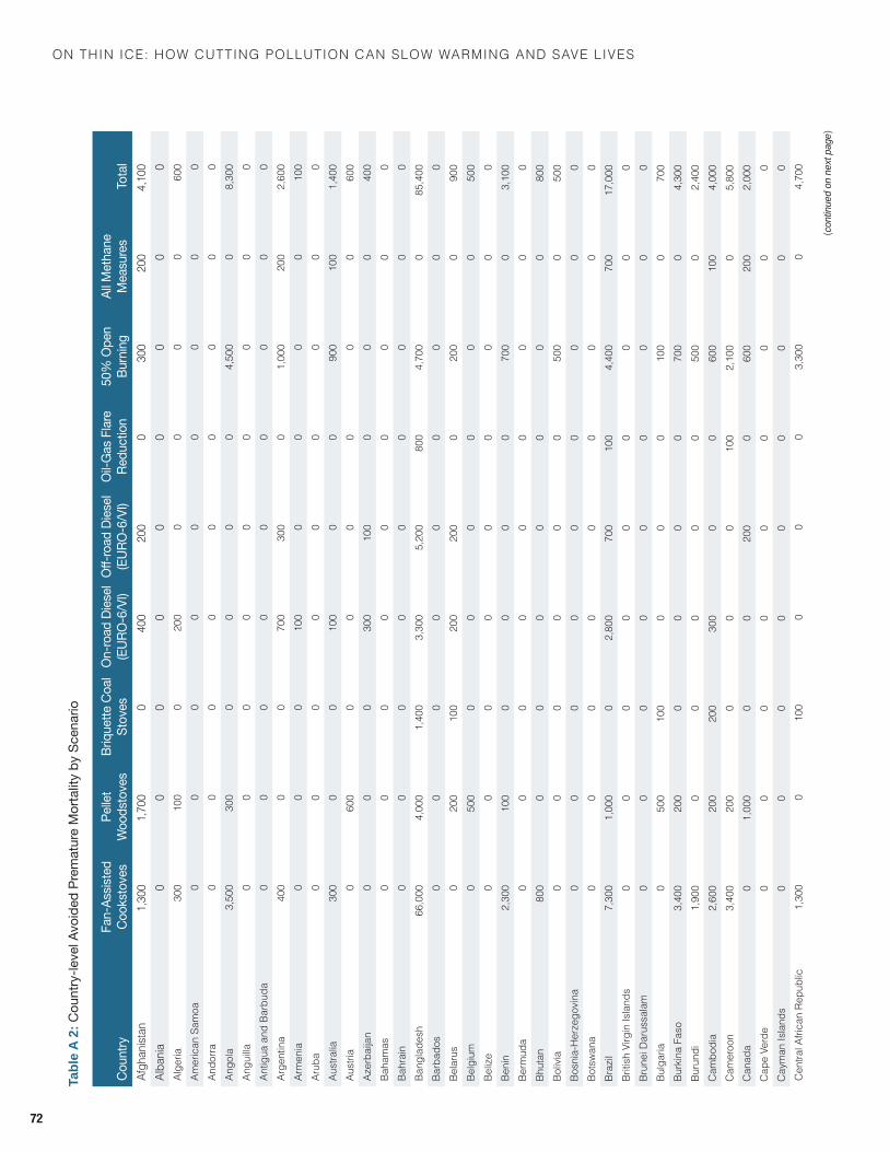
On thin ice: hOw cutting pOllutiOn can slOw warming and save lives
72
(con
tinue
d on
nex
t pag
e)
Tabl
e A
2: C
ount
ry-le
vel A
void
ed P
rem
atur
e M
orta
lity
by S
cena
rio
Coun
tryFa
n-As
siste
d Co
okst
oves
Pelle
t W
oods
tove
sBr
ique
tte C
oal
Stov
esOn
-road
Dies
el (E
URO-
6/VI
)Off
-roadDies
el(E
URO-
6/VI
)Oi
l-Gas
Flar
e Re
duct
ion
50%
Ope
n Bu
rnin
gAl
l Met
hane
M
easu
res
Tota
laf
ghan
istan
1,30
01,
700
040
020
00
300
200
4,10
0al
bani
a0
00
00
00
00
alge
ria30
010
00
200
00
00
600
amer
ican
sam
oa0
00
00
00
00
ando
rra0
00
00
00
00
ango
la3,
500
300
00
00
4,50
00
8,30
0an
guilla
00
00
00
00
0an
tigua
and
Bar
buda
00
00
00
00
0ar
gent
ina
400
00
700
300
01,
000
200
2,60
0ar
men
ia0
00
100
00
00
100
arub
a0
00
00
00
00
aust
ralia
300
00
100
00
900
100
1,40
0au
stria
060
00
00
00
060
0Az
erba
ijan
00
030
010
00
00
400
Baha
mas
00
00
00
00
0Ba
hrai
n0
00
00
00
00
Bang
lade
sh66
,000
4,00
01,
400
3,30
05,
200
800
4,70
00
85,4
00Ba
rbad
os0
00
00
00
00
Bela
rus
020
010
020
020
00
200
090
0Be
lgiu
m0
500
00
00
00
500
Beliz
e0
00
00
00
00
Beni
n2,
300
100
00
00
700
03,
100
Berm
uda
00
00
00
00
0Bh
utan
800
00
00
00
080
0Bo
livia
00
00
00
500
050
0Bo
snia
-Her
zego
vina
00
00
00
00
0Bo
tsw
ana
00
00
00
00
0Br
azil
7,30
01,
000
02,
800
700
100
4,40
070
017
,000
Briti
sh v
irgin
Isla
nds
00
00
00
00
0Br
unei
dar
ussa
lam
00
00
00
00
0Bu
lgar
ia0
500
100
00
010
00
700
Burk
ina
faso
3,40
020
00
00
070
00
4,30
0Bu
rund
i1,
900
00
00
050
00
2,40
0C
ambo
dia
2,60
020
020
030
00
060
010
04,
000
Cam
eroo
n3,
400
200
00
010
02,
100
05,
800
Can
ada
01,
000
00
200
060
020
02,
000
Cap
e ve
rde
00
00
00
00
0C
aym
an Is
land
s0
00
00
00
00
Cen
tral a
frica
n re
publ
ic1,
300
010
00
00
3,30
00
4,70
0
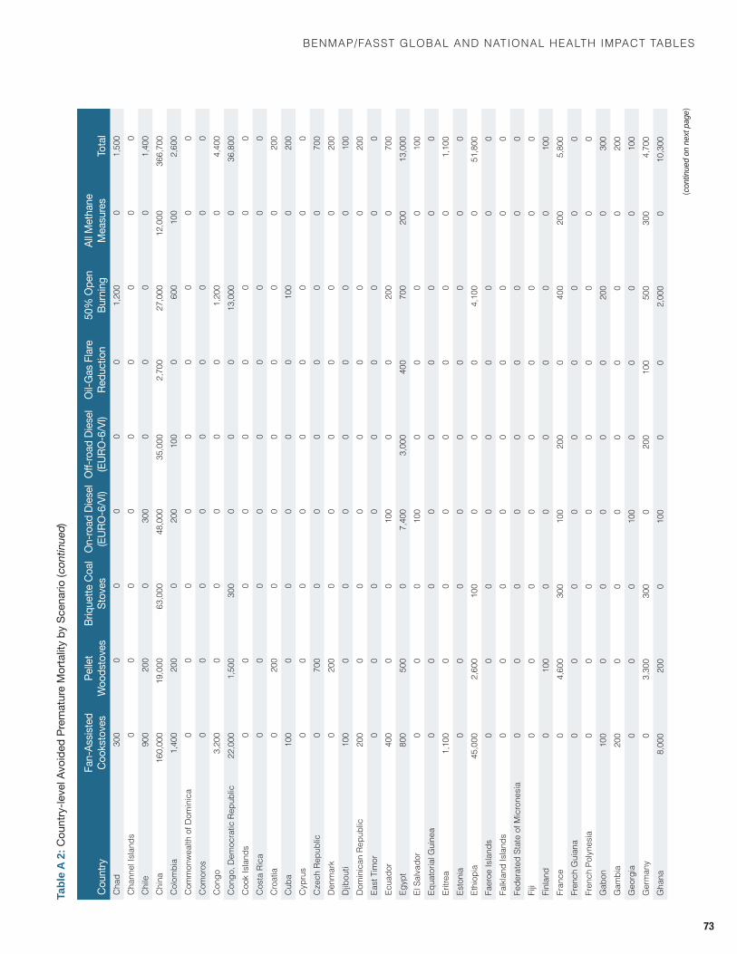
BenmaP/fasst GloBal and natIonal health ImPaCt taBles
73
Tabl
e A
2: C
ount
ry-le
vel A
void
ed P
rem
atur
e M
orta
lity
by S
cena
rio (c
ontin
ued)
(con
tinue
d on
nex
t pag
e)
Cha
d30
00
00
00
1,20
00
1,50
0C
hann
el Is
land
s0
00
00
00
00
Chi
le90
020
00
300
00
00
1,40
0C
hina
160,
000
19,0
0063
,000
48,0
0035
,000
2,70
027
,000
12,0
0036
6,70
0C
olom
bia
1,40
020
00
200
100
060
010
02,
600
Com
mon
wea
lth o
f dom
inic
a0
00
00
00
00
Com
oros
00
00
00
00
0C
ongo
3,20
00
00
00
1,20
00
4,40
0C
ongo
, dem
ocra
tic r
epub
lic22
,000
1,50
030
00
00
13,0
000
36,8
00C
ook
Isla
nds
00
00
00
00
0C
osta
ric
a0
00
00
00
00
Cro
atia
020
00
00
00
020
0C
uba
100
00
00
010
00
200
Cyp
rus
00
00
00
00
0C
zech
Rep
ublic
070
00
00
00
070
0d
enm
ark
020
00
00
00
020
0d
jibou
ti10
00
00
00
00
100
dom
inic
an r
epub
lic20
00
00
00
00
200
east
tim
or0
00
00
00
00
ecua
dor
400
00
100
00
200
070
0eg
ypt
800
500
07,
400
3,00
040
070
020
013
,000
el s
alva
dor
00
010
00
00
010
0eq
uato
rial G
uine
a0
00
00
00
00
eritr
ea1,
100
00
00
00
01,
100
esto
nia
00
00
00
00
0et
hiop
ia45
,000
2,60
010
00
00
4,10
00
51,8
00fa
eroe
Isla
nds
00
00
00
00
0fa
lkla
nd Is
land
s0
00
00
00
00
fede
rate
d st
ate
of m
icro
nesi
a0
00
00
00
00
fiji
00
00
00
00
0fi
nlan
d0
100
00
00
00
100
fran
ce0
4,60
030
010
020
00
400
200
5,80
0fr
ench
Gui
ana
00
00
00
00
0fr
ench
Pol
ynes
ia0
00
00
00
00
Gab
on10
00
00
00
200
030
0G
ambi
a20
00
00
00
00
200
Geo
rgia
00
010
00
00
010
0G
erm
any
03,
300
300
020
010
050
030
04,
700
Gha
na8,
000
200
010
00
02,
000
010
,300
Coun
tryFa
n-As
siste
d Co
okst
oves
Pelle
t W
oods
tove
sBr
ique
tte C
oal
Stov
esOn
-road
Dies
el (E
URO-
6/VI
)Off
-roadDies
el(E
URO-
6/VI
)Oi
l-Gas
Flar
e Re
duct
ion
50%
Ope
n Bu
rnin
gAl
l Met
hane
M
easu
res
Tota
l
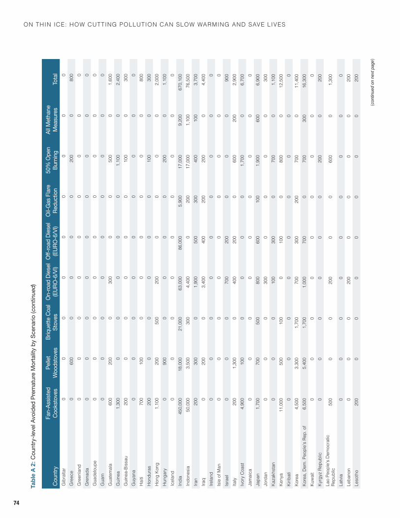
On thin ice: hOw cutting pOllutiOn can slOw warming and save lives
74
Tabl
e A
2: C
ount
ry-le
vel A
void
ed P
rem
atur
e M
orta
lity
by S
cena
rio (c
ontin
ued)
Coun
tryFa
n-As
siste
d Co
okst
oves
Pelle
t W
oods
tove
sBr
ique
tte C
oal
Stov
esOn
-road
Dies
el (E
URO-
6/VI
)Off
-roadDies
el(E
URO-
6/VI
)Oi
l-Gas
Flar
e Re
duct
ion
50%
Ope
n Bu
rnin
gAl
l Met
hane
M
easu
res
Tota
lG
ibra
ltar
00
00
00
00
0G
reec
e0
600
00
00
200
080
0G
reen
land
00
00
00
00
0G
rena
da0
00
00
00
00
Gua
delo
upe
00
00
00
00
0G
uam
00
00
00
00
0G
uate
mal
a60
020
00
300
00
500
01,
600
Gui
nea
1,30
00
00
00
1,10
00
2,40
0G
uine
a-Bi
ssau
200
00
00
010
00
300
Guy
ana
00
00
00
00
0h
aiti
700
100
00
00
00
800
hon
dura
s20
00
00
00
100
030
0h
ong
Kong
1,10
020
050
020
00
00
02,
000
hun
gary
090
00
00
020
00
1,10
0Ic
elan
d0
00
00
00
00
Indi
a45
0,00
018
,000
21,0
0063
,000
86,0
005,
900
17,0
009,
200
670,
100
Indo
nesi
a50
,000
3,50
030
04,
400
020
017
,000
1,10
076
,500
Iran
200
300
01,
900
500
300
400
100
3,70
0Ira
q0
200
03,
400
400
200
200
04,
400
Ir ela
nd0
00
00
00
00
Isle
of m
an0
00
00
00
00
Isra
el0
00
700
200
00
090
0Ita
ly20
01,
300
040
020
00
600
200
2,90
0Iv
ory
Coa
st4,
900
100
00
00
1,70
00
6,70
0Ja
mai
ca0
00
00
00
00
Japa
n1,
700
700
500
800
600
100
1,90
060
06,
900
Jor d
an0
00
300
00
00
300
Kaza
khst
an0
00
100
300
070
00
1,10
0Ke
nya
11,0
0050
010
00
100
080
00
12,5
00Ki
ribat
i0
00
00
00
00
Kore
a4,
500
3,30
01,
700
700
300
200
700
011
,400
Kore
a, d
em. P
eopl
e's
rep.
of
6,50
05,
400
1,70
01,
000
700
070
030
016
,300
Kuw
ait
00
00
00
00
0Ky
rgyz
Rep
ublic
00
00
00
200
020
0la
o Pe
ople
's d
emoc
ratic
re
publ
ic50
00
020
00
060
00
1,30
0
latv
ia0
00
00
00
00
leba
non
00
020
00
00
020
0le
soth
o20
00
00
00
00
200
(con
tinue
d on
nex
t pag
e)
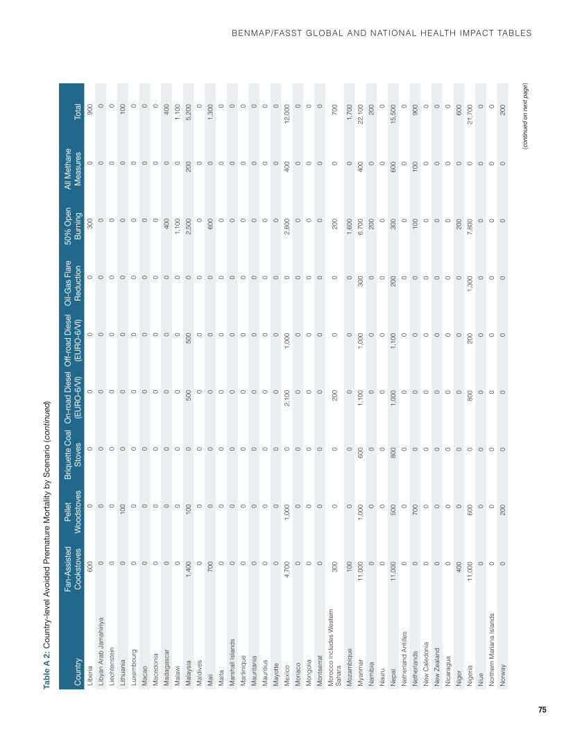
BenmaP/fasst GloBal and natIonal health ImPaCt taBles
75
Tabl
e A
2: C
ount
ry-le
vel A
void
ed P
rem
atur
e M
orta
lity
by S
cena
rio (c
ontin
ued)
Coun
tryFa
n-As
siste
d Co
okst
oves
Pelle
t W
oods
tove
sBr
ique
tte C
oal
Stov
esOn
-road
Dies
el (E
URO-
6/VI
)Off
-roadDies
el(E
URO-
6/VI
)Oi
l-Gas
Flar
e Re
duct
ion
50%
Ope
n Bu
rnin
gAl
l Met
hane
M
easu
res
Tota
lli
beria
600
00
00
030
00
900
liby
an a
rab
Jam
ahiri
ya0
00
00
00
00
liec
hten
stei
n0
00
00
00
00
lith
uani
a0
100
00
00
00
100
Luxe
mbo
urg
00
00
00
00
0m
acao
00
00
00
00
0m
aced
onia
00
00
00
00
0m
adag
asca
r0
00
00
040
00
400
mal
awi
00
00
00
1,10
00
1,10
0m
alay
sia
1,40
010
00
500
500
02,
500
200
5,20
0m
aldi
ves
00
00
00
00
0m
ali
700
00
00
060
00
1,30
0m
alta
00
00
00
00
0m
arsh
all I
slan
ds0
00
00
00
00
mar
tiniq
ue0
00
00
00
00
mau
ritan
ia0
00
00
00
00
mau
ritiu
s0
00
00
00
00
may
otte
00
00
00
00
0M
exic
o4,
700
1,00
00
2,10
01,
000
02,
800
400
12,0
00m
onac
o0
00
00
00
00
mon
golia
00
00
00
00
0m
onts
erra
t0
00
00
00
00
mor
occo
incl
udes
wes
tern
sa
hara
300
00
200
00
200
070
0
Moz
ambi
que
100
00
00
01,
600
01,
700
mya
nmar
11,0
001,
000
600
1,10
01,
000
300
6,70
040
022
,100
nam
ibia
00
00
00
200
020
0n
auru
00
00
00
00
0n
epal
11,0
0050
080
01,
000
1,10
020
030
060
015
,500
net
herla
nd a
ntille
s0
00
00
00
00
net
herla
nds
070
00
00
010
010
090
0n
ew C
aled
onia
00
00
00
00
0n
ew Z
eala
nd0
00
00
00
00
nic
arag
ua0
00
00
00
00
nig
er40
00
00
00
200
060
0n
iger
ia11
,000
600
080
020
01,
300
7,80
00
21,7
00n
iue
00
00
00
00
0n
orth
ern
mar
iana
Isla
nds
00
00
00
00
0n
orw
ay0
200
00
00
00
200
(con
tinue
d on
nex
t pag
e)
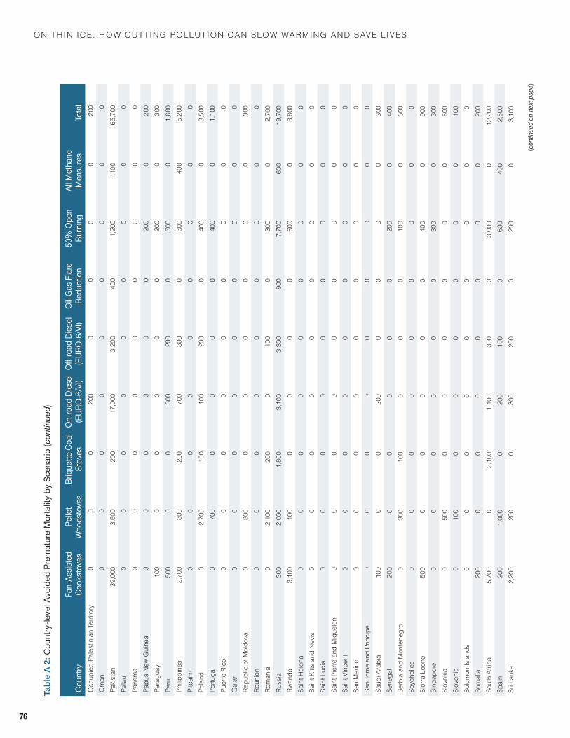
On thin ice: hOw cutting pOllutiOn can slOw warming and save lives
76
Tabl
e A
2: C
ount
ry-le
vel A
void
ed P
rem
atur
e M
orta
lity
by S
cena
rio (c
ontin
ued)
Coun
tryFa
n-As
siste
d Co
okst
oves
Pelle
t W
oods
tove
sBr
ique
tte C
oal
Stov
esOn
-road
Dies
el (E
URO-
6/VI
)Off
-roadDies
el(E
URO-
6/VI
)Oi
l-Gas
Flar
e Re
duct
ion
50%
Ope
n Bu
rnin
gAl
l Met
hane
M
easu
res
Tota
lo
ccup
ied
Pale
stin
ian
terri
tory
00
020
00
00
020
0o
man
00
00
00
00
0Pa
kist
an39
,000
3,60
020
017
,000
3,20
040
01,
200
1,10
065
,700
Pala
u0
00
00
00
00
Pana
ma
00
00
00
00
0Pa
pua
new
Gui
nea
00
00
00
200
020
0Pa
ragu
ay10
00
00
00
200
030
0Pe
ru50
00
030
020
00
600
01,
600
Philip
pine
s2,
700
300
200
700
300
060
040
05,
200
Pitc
airn
00
00
00
00
0Po
land
02,
700
100
100
200
040
00
3,50
0Po
rtuga
l0
700
00
00
400
01,
100
Puer
to r
ico
00
00
00
00
0Q
atar
00
00
00
00
0re
publ
ic o
f mol
dova
030
00
00
00
030
0re
unio
n0
00
00
00
00
rom
ania
02,
100
200
010
00
300
02,
700
russ
ia30
02,
000
1,80
03,
100
3,30
090
07,
700
600
19,7
00rw
anda
3,10
010
00
00
060
00
3,80
0sa
int h
elen
a0
00
00
00
00
sain
t Kitt
s an
d n
evis
00
00
00
00
0sa
int l
ucia
00
00
00
00
0sa
int P
ierre
and
miq
uelo
n0
00
00
00
00
sain
t vin
cent
00
00
00
00
0sa
n m
arin
o0
00
00
00
00
sao
tom
e an
d Pr
inci
pe0
00
00
00
00
saud
i ara
bia
100
00
200
00
00
300
sene
gal
200
00
00
020
00
400
serb
ia a
nd m
onte
negr
o0
300
100
00
010
00
500
seyc
helle
s0
00
00
00
00
sier
ra l
eone
500
00
00
040
00
900
sing
apor
e0
00
00
030
00
300
slov
akia
050
00
00
00
050
0sl
oven
ia0
100
00
00
00
100
solo
mon
Isla
nds
00
00
00
00
0so
mal
ia20
00
00
00
00
200
sout
h af
rica
5,70
00
2,10
01,
100
300
03,
000
012
,200
spai
n20
01,
000
020
010
00
600
400
2,50
0sr
i lan
ka2,
200
200
030
020
00
200
03,
100
(con
tinue
d on
nex
t pag
e)
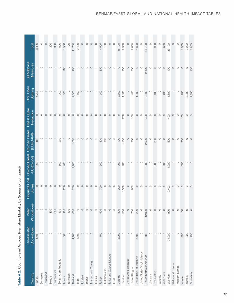
BenmaP/fasst GloBal and natIonal health ImPaCt taBles
77
Tabl
e A
2: C
ount
ry-le
vel A
void
ed P
rem
atur
e M
orta
lity
by S
cena
rio (c
ontin
ued)
Coun
tryFa
n-As
siste
d Co
okst
oves
Pelle
t W
oods
tove
sBr
ique
tte C
oal
Stov
esOn
-road
Dies
el (E
URO-
6/VI
)Off
-roadDies
el(E
URO-
6/VI
)Oi
l-Gas
Flar
e Re
duct
ion
50%
Ope
n Bu
rnin
gAl
l Met
hane
M
easu
res
Tota
lsu
dan
1,40
00
020
010
00
1,70
00
3,40
0su
rinam
e0
00
00
00
00
Swaz
iland
00
00
00
00
0sw
eden
030
00
00
00
030
0Sw
itzer
land
030
00
00
00
030
0sy
rian
arab
rep
ublic
010
00
500
200
020
00
1,00
0ta
iwan
500
100
200
400
00
100
200
1,50
0ta
jikis
tan
010
00
00
00
010
0th
aila
nd4,
100
800
200
2,70
01,
000
02,
500
400
11,7
00to
go1,
800
00
00
060
00
2,40
0to
kela
u0
00
00
00
00
tong
a0
00
00
00
00
trin
idad
and
tob
ago
00
00
00
00
0tu
nisi
a0
00
00
00
00
turk
ey10
090
070
060
080
00
600
300
4,00
0tu
rkm
enis
tan
00
00
100
00
010
0tu
rks
and
Cai
cos
Isla
nds
00
00
00
00
0tu
valu
00
00
00
00
0U
gand
a12
,000
800
200
200
100
02,
800
016
,100
Ukr
aine
01,
500
1,30
090
01,
100
200
1,10
020
06,
300
Uni
ted
arab
em
irate
s0
00
00
00
00
Uni
ted
King
dom
070
060
00
200
100
400
600
2,60
0U
nite
d Re
p. o
f Tan
zani
a2,
700
200
00
00
1,90
00
4,80
0U
nite
d st
ates
virg
in Is
land
s0
00
00
00
00
Uni
ted
stat
es o
f am
eric
a70
012
,000
060
02,
600
400
6,30
02,
100
24,7
00U
rugu
ay0
00
00
00
00
Uzb
ekis
tan
010
00
200
200
040
00
900
vanu
atu
00
00
00
00
0Ve
nezu
ela
00
020
00
040
00
600
viet
nam
24,0
001,
900
2,40
01,
900
500
400
1,60
040
033
,100
wal
lis a
nd f
utun
a0
00
00
00
00
wes
tern
sam
oa0
00
00
00
00
yem
en80
010
00
500
200
100
200
01,
900
Zam
bia
200
00
00
02,
000
02,
200
Zim
babw
e20
00
00
00
1,50
010
01,
800

79
Modeling Methods and Parameters
Background
An integrated suite of models was used to analyze the effects of individual pollution emissions control measures on a number of indicators related to cryosphere impacts and development. Details for each step in the process are described here. This work follows on the methods established in the UNEP/WMO Integrated Assessment of Black Carbon and Tropospheric Ozone (2011) and Shindell et al. (2012).
Emissions
The effects of emission control measures were estimated using the GAINS (Greenhouse gas—Air Pollution Interactions and Synergies) model, developed by the International Institute for Applied Systems Analysis (IIASA). This model brings together information on cur-rent and future economic, energy, and agricultural development, emission control potentials and costs, atmospheric dispersion, and environmental sensitivities toward air pollution (Amann et al. 2011). These impacts are considered in a multi-pollutant context, quantifying the contributions of SO2, NOx, NH3, NMVOC, CO, and emissions of primary particulate matter and discriminating between fine and coarse particles as well as black carbon (BC) and organic carbon (OC). GAINS also accounts for emissions of six greenhouse gases that are included in the Kyoto protocol (CO2, CH4, N2O, and the three F-gases). The GAINS model is implemented as an interactive web-based tool and is freely available over the internet (http://gains.iiasa.ac.at).
In this analysis, GAINS has been used to estimate baseline emissions (for details of the baseline scenario see (UNEP/WMO 2011) and the abatement potential of measures addressing primarily short-lived climate forcers. GAINS includes ~1650 measures with different individual impacts on emissions which can be grouped into ~400 broader categories of measures, such as those used here (e.g., EURO-6/VI on diesel cars, on light duty trucks, and on heavy duty trucks have distinct effects on
emissions but can all be categorized as part of a diesel vehicle measure).
Prior investigation identified 16 specific measures with a high potential for providing benefits both in terms of mitigation of global warming and reduction of air pollution (UNEP 2011). As the effects of methane emissions are the same regardless of the emis-sion location, and the identified methane sources have minimal co-emissions, previous analyses are adequate to characterize the forcing impacts of the seven identified methane measures. They have been reported previously (Shindell et al. 2012). The analysis presented here focuses on the BC-related measures, incorporating many of the nine measures previously identified for reducing emis-sions of products of incomplete combustion (BC, OC, CO, etc.), as well as some additions and modifications (Table A3). For the cookstove measures, these include a more rigorous evaluation of the emissions from either improved replacement cookstoves or alternative cookstoves using modern fuels, as in (UNEP 2011), rather than the simpler removal of emissions in the UNEP/WMO Integrated Assessment (2011). The 14 measures examined here incorporate most of the prior measures and include mitigation of associated gas flared at oil and gas production fields and targeted reduction of open biomass burning stemming from agricultural fires in central Eurasia or globally.
For the reduction of open biomass burning stemming from agricultural fires in Eurasia to EU levels, the report analyzes fire counts observed by the satellite-borne MODIS instrument over 2005–2008; it then uses the land-use dataset of Ramankutty et al. (2008) to determine the fire count per km2 of agricultural land per year. The report then uses the emissions inventory GFED3,1 also based on satellite observations, to determine the ratio of emissions per km2 of agricultural land per year for the study region (using the Former Soviet Union as a proxy) as compared with the EU, obtaining a value of 12.3. Hence the best practice for agricultural burning was determined to be eight percent of the current FSU level. This value was applied to all fires from 45–60°N, 30–140°E on the assumption that in this area many of the wildfires are started from agricultural burning. A second open burning simulation
Annex 2
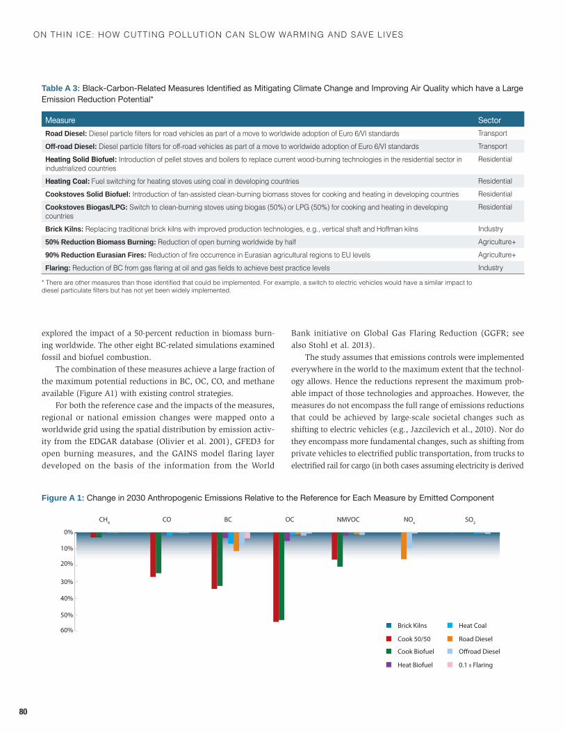
On thin ice: hOw cutting pOllutiOn can slOw warming and save lives
80
explored the impact of a 50-percent reduction in biomass burn-ing worldwide. The other eight BC-related simulations examined fossil and biofuel combustion.
The combination of these measures achieve a large fraction of the maximum potential reductions in BC, OC, CO, and methane available (Figure A1) with existing control strategies.
For both the reference case and the impacts of the measures, regional or national emission changes were mapped onto a worldwide grid using the spatial distribution by emission activ-ity from the EDGAR database (Olivier et al. 2001), GFED3 for open burning measures, and the GAINS model flaring layer developed on the basis of the information from the World
Bank initiative on Global Gas Flaring Reduction (GGFR; see also Stohl et al. 2013).
The study assumes that emissions controls were implemented everywhere in the world to the maximum extent that the technol-ogy allows. Hence the reductions represent the maximum prob-able impact of those technologies and approaches. However, the measures do not encompass the full range of emissions reductions that could be achieved by large-scale societal changes such as shifting to electric vehicles (e.g., Jazcilevich et al., 2010). Nor do they encompass more fundamental changes, such as shifting from private vehicles to electrified public transportation, from trucks to electrified rail for cargo (in both cases assuming electricity is derived
Table A 3:Black-Carbon-RelatedMeasuresIdentifiedasMitigatingClimateChangeandImprovingAirQualitywhichhaveaLargeEmission Reduction Potential*
Measure SectorRoad Diesel: Diesel particle filters for road vehicles as part of a move to worldwide adoption of Euro 6/VI standards transportOff-road Diesel: Diesel particle filters for off-road vehicles as part of a move to worldwide adoption of Euro 6/VI standards transportHeatingSolidBiofuel: Introduction of pellet stoves and boilers to replace current wood-burning technologies in the residential sector in industrialized countries
residential
HeatingCoal:fuel switching for heating stoves using coal in developing countries residentialCookstoves Solid Biofuel: Introduction of fan-assisted clean-burning biomass stoves for cooking and heating in developing countries residentialCookstoves Biogas/LPG: Switch to clean-burning stoves using biogas (50%) or LPG (50%) for cooking and heating in developing countries
residential
Brick Kilns: replacing traditional brick kilns with improved production technologies, e.g., vertical shaft and hoffman kilns Industry50% Reduction Biomass Burning: reduction of open burning worldwide by half agriculture+90% Reduction Eurasian Fires: Reduction of fire occurrence in Eurasian agricultural regions to EU levels agriculture+Flaring: Reduction of BC from gas flaring at oil and gas fields to achieve best practice levels Industry
* There are other measures than those identified that could be implemented. For example, a switch to electric vehicles would have a similar impact to diesel particulate filters but has not yet been widely implemented.
Figure A 1: Change in 2030 Anthropogenic Emissions Relative to the Reference for Each Measure by Emitted Component
0%
60%
10%
20%
30%
40%
50%
CH4 CO BC OC NMVOC NOx SO2
Brick Kilns
Cook 50/50
Cook Biofuel
Heat Biofuel
Heat Coal
Road Diesel
O�road Diesel
0.1 X Flaring
0%
60%
10%
20%
30%
40%
50%
CH4 CO BC OC NMVOC NOx SO2
Brick Kilns
Cook 50/50
Cook Biofuel
Heat Biofuel
Heat Coal
Road Diesel
O�road Diesel
0.1 X Flaring
modelInG methods and Parameters
81
from clean sources), enhanced standards (e.g., fuel economy), or dramatically greater use of renewables (including natural gas) rather than fossil fuels. (e.g., Delucchi and Jacobsen 2011). Hence further work could usefully characterize the choices available to policymakers in particular regions based on these various other considerations aside from mitigation of global climate change through technical measures, and could quite reasonably come up with mitigation potential substantially larger than that found here.
Composition-Climate Models
The emissions changes associated with the ten control measures provide input to global three-dimensional composition-climate models to calculate their impact on radiative forcing and surface air pollutants. To characterize the sensitivity of the results to uncertainties in the representation of physical processes, multiple independent models are used.
The study uses the GISS model for Physical Understanding of Composition-Climate INteractions and Impacts (GISS-PUCCINI), which incorporates gas-phase, sulfate, black carbon, nitrate, and secondary organic aerosol chemistry within the GISS ModelE2 general circulation model. The study uses the most recent docu-mented version of this model, that used for the Coupled Model Intercomparison Project Phase 5 (CMIP5) and Atmospheric Chemistry and Climate Model Intercomparison Project (ACCMIP), hereafter referred to as GISS-E2, for which the behavior of gases and aerosols has been documented extensively (e.g., Shindell et al. 2013 a, b). The model finds pre-industrial to present-day ozone forcing on the low side of the range in other models, underes-timates present-day global mean aerosol optical depths weakly (8–14 percent) relative to ground-based and satellite observations (the underestimate is ~35 percent for East Asia), and, like most models, appears to underestimate absorbing aerosol optical depth by roughly a factor of two. The total aerosol effective radiative forcing (direct plus indirect) in this model is in reasonable agree-ment with other CMIP5 models—though, like the other models, it is a larger negative value than that inferred from estimates constrained with modern satellite data (e.g., Quaas et al. 2008; Christensen and Stephens 2011). The model has a horizontal resolution of 2° latitude by 2.5° longitude, with increased effec-tive resolution for tracers due to carrying higher order moments at each grid box. This configuration had 40 vertical hybrid sigma layers from the surface to 0.1 hPa. Gas-phase chemistry includes 51 chemical species interacting via 156 reactions. The model includes sulfate, nitrate, carbonaceous (black and organic, both primary and secondary for the latter), mineral dust, and sea salt. Tracer transport uses a non-diffusive quadratic upstream scheme (Prather 1986). Prescribed ocean simulations were performed using observed 2000-era sea-surface temperatures (Rayner et al. 2003),
with most runs extended for 40 years to allow accurate diagnoses of aerosol indirect effects. In comparison with the version of the GISS-E2 model used in prior studies, the current model incorpo-rates a more complete treatment of BC albedo forcing, including all snow and ice surfaces.
Coupled atmosphere-ocean runs were also performed using the GISS-E2-R version of that climate model. Those simulations, whose results are described in the climate impacts section, con-sisted of a control simulation with reference to 2030 conditions and a simulation incorporating half the methane reduction measures analyzed here. The coupled ocean-atmosphere model was run for 78 years with analysis carried out over the last 58 (i.e., excluding the initial equilibration of the model, though full equilibration of the deep ocean can in fact take centuries).
The study performed simulations with a second version of the GISS model that uses the same atmospheric model but has very different, independent aerosol model called the Two-Moment Aerosol Sectional (TOMAS) aerosol microphysics model (Lee et al. 2014, in preparation). The GISS-E2-TOMAS version has the same basic physics and resolution as the GISS-E2 model, but this model predicts aerosol number and mass size distributions by computing total aerosol number (i.e., 0th moment) and mass (i.e., 1st moment) concentrations for each species (sulfate, sea-salt, internally mixed elemental carbon, externally mixed elemental carbon, hydrophilic organic matter, hydrophobic organic matter, mineral dust, and aerosol-water) in 12-size bins ranging from 10 nm to 10 µm in dry diameter (Lee and Adams 2012). The model thus has 108 size-resolved aerosol tracers plus three bulk aerosol-phase and five bulk gas-phase species (versus 15 aerosol tracers in GISS-E2). Water uptake by sulfate, sea-salt, and hydro-philic organic matter is accounted for in the model. The tracer transport scheme and gas-phase chemistry are nearly the same as in GISS-E2, except that in GISS-E2-TOMAS, aerosols do not affect photolysis rates, a simpler representation of SOA is used, and nitrate chemistry is not included. The deposition scheme is basically the same as that in GISS-E2 except that size-resolved deposition processes are used for aerosols (Lee and Adams 2012). For example, modified Köhler theory is applied for aerosol in-cloud scavenging, and a size-dependent gravitational settling of particles and a size-dependent resistance in the quasi-laminar sublayer are used. Due to the much greater complexity of this aerosol model, it is significantly more computationally expensive than the simpler mass-based GISS-E2 model, and hence only a few measures could be examined with this version.
The study uses a fully coupled photochemistry-aerosol-climate model ECHAM5-HAMMOZ, which is based on the general circula-tion model (GCM) ECHAM5, developed at the Max Planck Institute for Meteorology (Pozzoli et al. 2008; Roeckner et al. 2006). The ECHAM5-HAMMOZ model (simply referred to as ECHAM in the following sections) is described in detail in Pozzoli et al. (2008). The
On thin ice: hOw cutting pOllutiOn can slOw warming and save lives
82
gas-phase chemical scheme has been adopted from the MOZART-2 model (Horowitz et al. 2003), and includes 63 transported tracers and 168 reactions to simulate O3 and the NOx-HOx-hydrocarbons chemistry. The aerosols are described by 7 log-normal modes. Four modes are considered as hydrophilic, internally-mixed, aerosols composed of sulfate, organic carbon (OC), black carbon (BC), mineral dust, sea salts, and water. Three additional modes are considered as hydrophobic aerosols, one composed of an internal mixture of BC and OC, and one of externally-mixed mineral dust (Stier et al. 2005; Vignati et al. 2004). Hence the ECHAM5-HAMMOZ aerosol model, in calculating both aerosol mass and number, is more similar to the GISS-E2-TOMAS model than the GISS-E2 model, although with less resolution of aerosol types/states. The sulfur chemistry and secondary sulfate aerosol production is described by Feichter et al. (1996), which includes oxidation of SO
2 by OH and DMS oxidation by OH and NO3. The emissions from vegeta-tion of CO and VOCs (e.g. isoprene and terpenes) are calculated interactively using the Model of Emissions of Gases and Aerosols from Nature (MEGAN) (Guenther et al., 2006).
The biogenic monoterpene emissions of Guenther et al. (1995) are scaled by the factor 0.15 to estimate the production of Secondary Organic Aerosol (SOA) from biogenic sources following Pozzoli et al. (2008). SOA is then injected in the atmosphere as primary organic aerosol. The ECHAM5-HAMMOZ model has been extensively evaluated in previous studies (Pozzoli et al., 2008 a, b; Pozzoli et al 2011; Stier et al. 2005; and Pausata et. al 2012) with comparisons to several measurements and to other model results. The simulated global annual average total aerosol optical depth (AOD) is slightly higher than the range of model/measurement values reported from Kinne et al. (2006). A good agreement is gen-erally found for PM2.5 concentrations measured at rural and urban stations. About 65 percent of the simulated PM2.5, downscaled with urban population, is in range of ± 25 percent with the measured urban background values in Europe (Pausata et al., 2013).
The tropospheric O3 budget and variability agree well with earlier multi-model comparison studies by Stevenson et al. (2006) and Hess and Mahowald (2009), while O3 surface concentrations are generally overestimated compared to ground based measure-ments. In this study, a T42 resolution was used, corresponding to an Eulerian resolution of ca. 2.8ºx2.8º, with 31 vertical levels from the surface up to 10 hPa and a time resolution for dynamics and a chemistry of 20 minutes. The transport scheme is from Lin and Rood (1996). In this project the large-scale meteorology is constrained to the year 2000, nudging the temperature, surface pressure, vorticity and divergence to the ECMWF (European Centre for Medium-range Weather Forecast) ERA40 reanalysis data. The radiative transfer calculation considers vertical profiles of the greenhouse gases (e.g., CO
2, O3, CH4), aerosols, and the cloud water and ice. The instanta-neous direct aerosol radiative forcing (RF) in ECHAM5-HAMMOZ is diagnostically calculated from the difference in the net radiative
fluxes including and excluding aerosol (Stier et al., 2007). Direct O3 RF is diagnosed using ECHAM5-HAMMOZ O3 columns, in combina-tion with all-sky radiative forcing efficiencies (Gauss et al., 2006).
Simulations were also performed with the HadGEM3 model (Hadley Centre Global Environment Model version 3). The configu-ration used here is “atmosphere-only,” using prescribed sea surface temperatures and sea ice distributions (Hewitt et al. 2011). The resolution is N90L63; 1.875°×1.25° horizontal resolution and 63 levels extending to ~40km height (of which 50 are below 18 km).
The gas-phase chemistry used is the UKCA TropIsop scheme treats 55 chemical species (37 of which are transported), includ-ing hydrocarbons up to propane, and isoprene and its degradation products (O’Connor et al. 2013). Atmospheric tracers (gas and aerosol) are advected using the same semi-Lagrangian advection scheme used for the physical climate variables. Parameterized transport (e.g., boundary layer and convection) is also as used for the physical climate variables.
The aerosol scheme used is UKCA-Mode (Mann et al. 2010; Abdul-Razzak and Ghan 2000). This models sulphate, organic carbon, black carbon, dust, and sea salt in an internally-mixed manner using a two-moment modal approach and dynamically evolving particle size distributions. Seven modes are used, four soluble (nucleation to coarse) and three insoluble (Aitken to coarse). Aerosol processes are simulated in a size-resolved man-ner, including primary emissions, secondary particle formation by binary homogeneous nucleation of sulfuric acid and water, particle growth by coagulation, condensation, and cloud-processing, and removal by dry deposition, in-cloud and below-cloud scavenging.
The radiative forcing from aerosols are calculated using the Edwards-Slingo radiation scheme. For the aerosol direct effect, the information on mean particle radius and composition for each of the internally-mixed size modes is used. A volume-average mix-ing rule is used over the components present (including water) to calculate the real and imaginary parts of the refractive index. The particle size determines the Mie parameter in relation to the wavelength. The look-up tables have been calculated based on the integrals across each of the spectral bands for the short-wave and long-wave used by HadGEM3. For the first indirect effect, the parameterization of Abdul-Razzak and Ghan (2000) is employed to calculate cloud droplet number concentration combining the online size distribution and composition information from UKCA-mode, with a cloud updraft velocity derived from the turbulent kinetic energy in the boundary layer.
The simulations performed by each model are summarized in Table A4. Each simulation refers to one of the BC-related measure listed in Table A3. Two additional scenarios were performed for solid biomass and coal heating stoves, including a monthly sea-sonal variation for heating stoves emissions (C2 and D2), versus the constant annual distribution (C1 and D1).
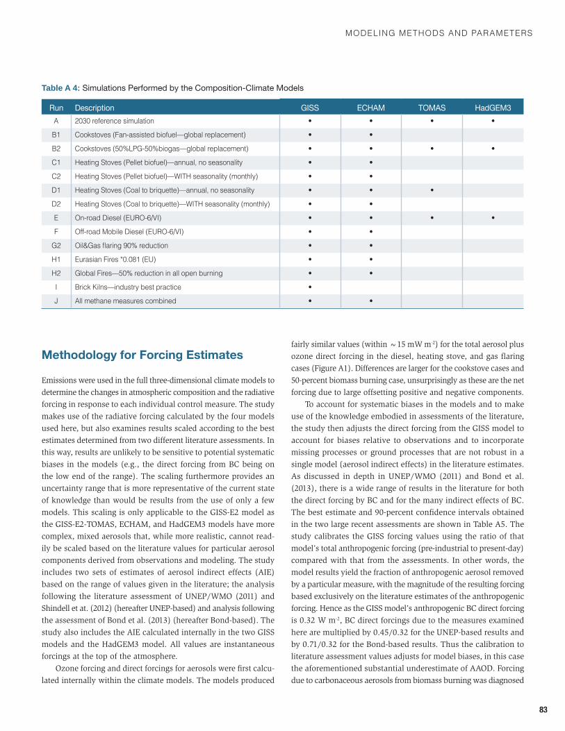
modelInG methods and Parameters
83
Methodology for Forcing Estimates
Emissions were used in the full three-dimensional climate models to determine the changes in atmospheric composition and the radiative forcing in response to each individual control measure. The study makes use of the radiative forcing calculated by the four models used here, but also examines results scaled according to the best estimates determined from two different literature assessments. In this way, results are unlikely to be sensitive to potential systematic biases in the models (e.g., the direct forcing from BC being on the low end of the range). The scaling furthermore provides an uncertainty range that is more representative of the current state of knowledge than would be results from the use of only a few models. This scaling is only applicable to the GISS-E2 model as the GISS-E2-TOMAS, ECHAM, and HadGEM3 models have more complex, mixed aerosols that, while more realistic, cannot read-ily be scaled based on the literature values for particular aerosol components derived from observations and modeling. The study includes two sets of estimates of aerosol indirect effects (AIE) based on the range of values given in the literature; the analysis following the literature assessment of UNEP/WMO (2011) and Shindell et at. (2012) (hereafter UNEP-based) and analysis following the assessment of Bond et al. (2013) (hereafter Bond-based). The study also includes the AIE calculated internally in the two GISS models and the HadGEM3 model. All values are instantaneous forcings at the top of the atmosphere.
Ozone forcing and direct forcings for aerosols were first calcu-lated internally within the climate models. The models produced
fairly similar values (within ~15 mW m-2) for the total aerosol plus ozone direct forcing in the diesel, heating stove, and gas flaring cases (Figure A1). Differences are larger for the cookstove cases and 50-percent biomass burning case, unsurprisingly as these are the net forcing due to large offsetting positive and negative components.
To account for systematic biases in the models and to make use of the knowledge embodied in assessments of the literature, the study then adjusts the direct forcing from the GISS model to account for biases relative to observations and to incorporate missing processes or ground processes that are not robust in a single model (aerosol indirect effects) in the literature estimates. As discussed in depth in UNEP/WMO (2011) and Bond et al. (2013), there is a wide range of results in the literature for both the direct forcing by BC and for the many indirect effects of BC. The best estimate and 90-percent confidence intervals obtained in the two large recent assessments are shown in Table A5. The study calibrates the GISS forcing values using the ratio of that model’s total anthropogenic forcing (pre-industrial to present-day) compared with that from the assessments. In other words, the model results yield the fraction of anthropogenic aerosol removed by a particular measure, with the magnitude of the resulting forcing based exclusively on the literature estimates of the anthropogenic forcing. Hence as the GISS model’s anthropogenic BC direct forcing is 0.32 W m-2, BC direct forcings due to the measures examined here are multiplied by 0.45/0.32 for the UNEP-based results and by 0.71/0.32 for the Bond-based results. Thus the calibration to literature assessment values adjusts for model biases, in this case the aforementioned substantial underestimate of AAOD. Forcing due to carbonaceous aerosols from biomass burning was diagnosed
Table A 4: Simulations Performed by the Composition-Climate Models
Run Description GISS ECHAM TOMAS HadGEM3a 2030 reference simulation • • • •
B1 Cookstoves (Fan-assisted biofuel—global replacement) • •
B2 Cookstoves (50%LPG-50%biogas—global replacement) • • • •
C1 Heating Stoves (Pellet biofuel)—annual, no seasonality • •
C2 Heating Stoves (Pellet biofuel)—WITH seasonality (monthly) • •
d1 Heating Stoves (Coal to briquette)—annual, no seasonality • • •
d2 Heating Stoves (Coal to briquette)—WITH seasonality (monthly) • •
e On-road Diesel (EURO-6/VI) • • • •
f Off-road Mobile Diesel (EURO-6/VI) • •
G2 Oil&Gas flaring 90% reduction • •
h1 Eurasian Fires *0.081 (EU) • •
h2 Global Fires—50% reduction in all open burning • •
I Brick Kilns—industry best practice •
J all methane measures combined • •
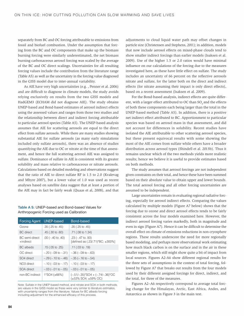
On thin ice: hOw cutting pOllutiOn can slOw warming and save lives
84
separately from BC and OC forcing attributable to emissions from fossil and biofuel combustion. Under the assumption that forc-ing from the BC and OC components that make up the biomass burning forcing were similarly underestimated, the net biomass burning carbonaceous aerosol forcing was scaled by the average of the BC and OC direct scalings. Uncertainties for all resulting forcing values include the contribution from the literature range (Table A5) as well as the uncertainty in the forcing value diagnosed in the GISS model due to inter-annual variability.
As AIE have very high uncertainties (e.g. , Penner et al. 2006) and are difficult to diagnose in climate models, the study avoids relying exclusively on results from the two GISS models and HadGEM3 (ECHAM did not diagnose AIE). The study obtains UNEP-based and Bond-based estimates of aerosol indirect effects using the assessed values and ranges from those two studies and the relationship between direct and indirect forcing attributable to particular aerosol species (Table A5). The UNEP-based analysis assumes that AIE for scattering aerosols are equal to the direct effect from sulfate aerosols. While there are many studies showing substantial AIE for sulfate aerosols (as many early simulations included only sulfate aerosols), there was an absence of studies quantifying the AIE due to OC or nitrate at the time of that assess-ment, and hence the full scattering aerosol AIE was assigned to sulfate. Dominance of sulfate in AIE is consistent with its greater solubility and mass relative to carbonaceous or nitrate aerosols. Calculations based on detailed modeling and observations suggest that the ratio of AIE to direct sulfate RF is 1.5 to 2.0 (Kvalevag and Mhyre 2007), but a lower value of 1.0 was used as recent analyses based on satellite data suggest that at least a portion of the AIE may in fact be fairly weak (Quaas et al, 2008), and that
adjustments to cloud liquid water path may offset changes in particle size (Christensen and Stephens, 2011); in addition, models that now include aerosol effects on mixed-phase clouds tend to show smaller indirect forcings than earlier models (Isaksen et al. 2009). Use of the higher 1.5 or 2.0 ratios would have minimal influence on our calculations of the forcing due to the measures investigated here, as these have little effect on sulfate. The study includes an uncertainty of 66 percent on the reflective aerosols nitrate and sulfate, for the latter both on the direct and indirect effects (for nitrate assuming their impact is only direct effects), based on a recent assessment (Isaksen et al. 2009).
For the Bond-based analysis, indirect effects are quite differ-ent, with a larger effect attributed to OC than SO4 and the effects of both these components each being larger than the total in the UNEP-based method (Table A5). In addition, there is a positive net indirect effect attributed to BC. Apportionment to particular species was based on aerosol mass in that assessment, and did not account for differences in solubility. Recent studies have isolated the AIE attributable to other scattering aerosol species, but these present equivocal results with some showing the most of the AIE comes from sulfate while others have a broader distribution across aerosol types (Shindell et al. 2013b). Thus it remains unclear which of the two methods yields more realistic results; hence we believe it is useful to provide estimates based on both methods.
The study assumes that aerosol forcings are not independent given constraints on their total, and hence these have been summed based on their absolute value to obtain upper and lower bounds. The total aerosol forcing and all other forcing uncertainties are assumed to be independent.
Large uncertainties remain in evaluating regional radiative forc-ing, especially for aerosol indirect effects. Comparing the values calculated by multiple models (Figure A7 below) shows that the forcing due to ozone and direct aerosol effects tends to be fairly consistent across the four models examined here. However, the indirect aerosol forcing varies markedly, both in magnitude and even in sign (Figure A7). Hence it can be difficult to determine the overall effect on climate of emissions reductions in non-cryosphere regions. These results underscore the need for more regionally based modeling, and perhaps more observational work estimating how much black carbon is on the surface and in the air in these smaller regions, which still might show quite a bit of impact from local sources. Figures A2-A6 show different regional results for the three sets of assumptions in the context of total forcing, fol-lowed by Figure A7 that breaks out results from the four models used by their different assigned forcings for direct, indirect, and the total, for three of the measures.
Figures A2–A6 respectively correspond to average total forc-ing change for the Himalayas, Arctic, East Africa, Andes, and Antarctica as shown in Figure 3 in the main text.
Table A 5: UNEP-based and Bond-based Values for Anthropogenic Forcing used as Calibration
Forcing Agent UNEP-based Bond-basedOzone .35 (.25 to .45) .35 (.25 to .45)BC direct .45 (.30 to .60) .71 (.08 to 1.34)BC semi-direct +indirect
.00 (–.40 to .40) .23 (–.47 to .93) [defined as (.23/.71)*BC; ±300%]
BC albedo .15 (.05 to .25) .11 (.03 to .19)oC direct –.20 (–.09 to –.31) –.36 (–.09 to –.63)so4 direct –.29 (–.10 to –.48) –.35 (–.16 to –.54)no3 direct –.10 (–.03 to –.17) –.10 (–.03 to –.17)soa direct –.03 (–.01 to –.05) –.03 (–.01 to –.05)non-BC indirect 1*SO4 (±66%) (–.51/–.35)*SO4 + (–.74/–.36)*OC
(±53% SO4; ±59% OC)
note: sulfate in the UneP-based method, and nitrate and soa in both methods, are values in the GIss model as these were very similar to literature estimates, with uncertainty ranges from the literature. values for BC albedo forcing including adjustment for the enhanced efficacy of this process.
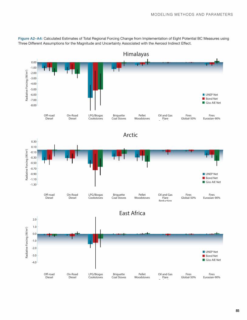
modelInG methods and Parameters
85
Figure A2–A4: Calculated Estimates of Total Regional Forcing Change from Implementation of Eight Potential BC Measures using ThreeDifferentAssumptionsfortheMagnitudeandUncertaintyAssociatedwiththeAerosolIndirectEffect.
Radi
ativ
e Fo
rcin
g (W
/m2 )
-3.00
-2.00
-1.00
0.00
-6.00
-5.00
-4.00
Himalayas
-7.00
-8.00
O�-roadDiesel
On-RoadDiesel
LPG/BiogasCookstoves
BriquetteCoal Stoves
PelletWoodstoves
Oil and GasFlare
Reduction
FiresGlobal-50%
FiresEurasian-90%
UNEP NetBond Net
Giss AIE Net
Radi
ativ
e Fo
rcin
g (W
/m2 )
-0.30
-0.10
0.10
0.30
-0.90
-0.70
-0.50
Arctic
-1.10
-1.30
O�-roadDiesel
On-RoadDiesel
LPG/BiogasCookstoves
BriquetteCoal Stoves
PelletWoodstoves
Oil and GasFlare
Reduction
FiresGlobal-50%
FiresEurasian-90%
UNEP NetBond Net
Giss AIE Net
Radi
ativ
e Fo
rcin
g (W
/m2 )
-1.0
0.0
1.0
2.0
-4.0
-3.0
-2.0
East Africa
O�-roadDiesel
On-RoadDiesel
LPG/BiogasCookstoves
BriquetteCoal Stoves
PelletWoodstoves
Oil and GasFlare
Reduction
FiresGlobal-50%
FiresEurasian-90%
UNEP NetBond Net
Giss AIE Net
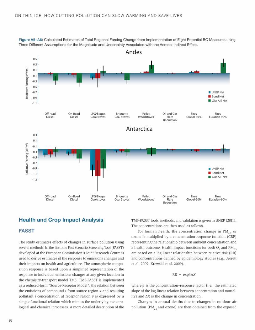
On thin ice: hOw cutting pOllutiOn can slOw warming and save lives
86
Health and Crop Impact Analysis
FASST
The study estimates effects of changes in surface pollution using several methods. In the first, the Fast Scenario Screening Tool (FASST) developed at the European Commission’s Joint Research Centre is used to derive estimates of the response to emissions changes and their impacts on health and agriculture. The atmospheric compo-sition response is based upon a simplified representation of the response to individual emissions changes at any given location in the chemistry-transport model TM5. TM5-FASST is implemented as a reduced-form “Source-Receptor Model”: the relation between the emissions of compound i from source region x and resulting pollutant j concentration at receptor region y is expressed by a simple functional relation which mimics the underlying meteoro-logical and chemical processes. A more detailed description of the
TM5-FASST tools, methods, and validation is given in UNEP (2011). The concentrations are then used as follows.
For human health, the concentration change in PM2.5 or ozone is multiplied by a concentration-response function (CRF) representing the relationship between ambient concentration and a health outcome. Health impact functions for both O3 and PM2.5 are based on a log-linear relationship between relative risk (RR) and concentrations defined by epidemiology studies (e.g., Jerrett et al. 2009; Krewski et al. 2009).
RR = expβΔX
where β is the concentration–response factor (i.e., the estimated slope of the log-linear relation between concentration and mortal-ity) and ΔX is the change in concentration.
Changes in annual deaths due to changes in outdoor air pollution (PM2.5 and ozone) are then obtained from the exposed
Figure A5–A6: Calculated Estimates of Total Regional Forcing Change from Implementation of Eight Potential BC Measures using ThreeDifferentAssumptionsfortheMagnitudeandUncertaintyAssociatedwiththeAerosolIndirectEffect.
Radi
ativ
e Fo
rcin
g (W
/m2 )
-0.1
0.1
0.3
0.5
-0.7
-0.9
-1.1
-0.5
-0.3
Andes
O�-roadDiesel
On-RoadDiesel
LPG/BiogasCookstoves
BriquetteCoal Stoves
PelletWoodstoves
Oil and GasFlare
Reduction
FiresGlobal-50%
FiresEurasian-90%
UNEP NetBond Net
Giss AIE Net
Radi
ativ
e Fo
rcin
g (W
/m2 )
-0.1
0.1
0.3
-0.7
-0.9
-1.1
-1.3
-0.5
-0.3
Antarctica
O�-roadDiesel
On-RoadDiesel
LPG/BiogasCookstoves
BriquetteCoal Stoves
PelletWoodstoves
Oil and GasFlare
Reduction
FiresGlobal-50%
FiresEurasian-90%
UNEP NetBond Net
Giss AIE Net
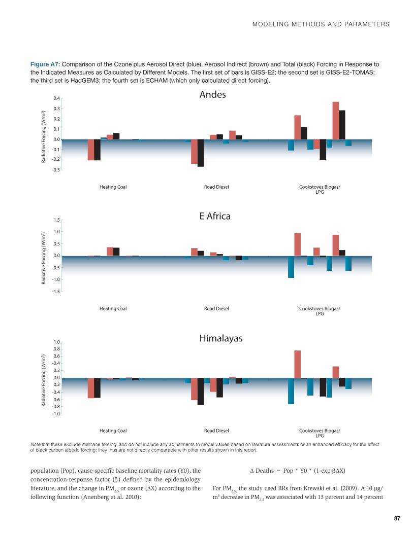
modelInG methods and Parameters
87
population (Pop), cause-specific baseline mortality rates (Y0), the concentration-response factor (β) defined by the epidemiology literature, and the change in PM2.5 or ozone (∆X) according to the following function (Anenberg et al. 2010):
∆ Deaths = Pop * Y0 * (1-exp-βΔX)
For PM2.5, the study used RRs from Krewski et al. (2009). A 10 μg/m3 decrease in PM2.5 was associated with 13 percent and 14 percent
Figure A7: Comparison of the Ozone plus Aerosol Direct (blue), Aerosol Indirect (brown) and Total (black) Forcing in Response to theIndicatedMeasuresasCalculatedbyDifferentModels.ThefirstsetofbarsisGISS-E2;thesecondsetisGISS-E2-TOMAS;the third set is HadGEM3; the fourth set is ECHAM (which only calculated direct forcing).
Note that these exclude methane forcing, and do not include any adjustments to model values based on literature assessments or an enhanced efficacy for the effect of black carbon albedo forcing; they thus are not directly comparable with other results shown in this report.
Radi
ativ
e Fo
rcin
g (W
/m2 )
0.2
0.3
0.4
-0.1
0.0
0.1
Andes
-0.2
-0.3
Heating Coal Road Diesel Cookstoves Biogas/LPG
Radi
ativ
e Fo
rcin
g (W
/m2 )
0.5
1.0
1.5
-0.5
0.0
E Africa
-1.0
-1.5
Heating Coal Road Diesel Cookstoves Biogas/LPG
Radi
ativ
e Fo
rcin
g (W
/m2 )
0.2
0.2
0.6
0.6
1.0
-0.4
-0.4
0.0
Himalayas
-0.8
0.8
-1.0
Heating Coal Road Diesel Cookstoves Biogas/LPG
On thin ice: hOw cutting pOllutiOn can slOw warming and save lives
88
decreases in cardiopulmonary and lung cancer mortality respec-tively. For ozone, the study based our health impact evaluation on the association between long-term O3 exposure and RR of death from respiratory disease found by (Jerrett et al. 2009), with RR = 4% increase in RR of death from respiratory disease for a 10bbpV increase in the maximum 6 monthly average daily 1-hr maximum O3.
The impact on agricultural yields is evaluated using the methodology of Van Dingenen et al. (2009), where the O3
concentration fields are now obtained with the TM5-FASST source-receptor model. The study overlays the ozone concentra-tion change with crop distribution maps and applies exposure-response functions derived from experiments that examine the yield reduction associated with different ozone concentrations. As in the UNEP/WMO Integrated Assessment, the relationship is based on the daylight ozone concentrations averaged over the growing-season, for four staple crops: wheat, rice, maize, and soybean. Relative yield losses (RYL) and crop production losses (CPL) are calculated from the crop production (CP) in a given historical year according to:
CPL = RYL/(1-RYL)*CP
BenMAP
Health impacts were also calculated using the U. S. EPA’s Envi-ronmental Benefits Mapping and Analysis Program (BenMAP). BenMAP is a Windows-based computer program that uses a Geographic Information System to estimate the health impacts and economic benefits occurring when populations experience changes in air quality.2 BenMAP provided estimates of avoided premature mortality associated with changes in ambient PM2.5
predicted by the different BC emissions scenarios, as well as all methane measures combined. The section below describes the data and health impact function used to generate these estimates, and presents both global and country-level results for each scenario. This methodology is similar to that employed in Anenberg et al. (2012).
Concentration-Response FunctionTo estimate PM2.5-related premature mortality, the study applies a concentration-response relationship from the Krewski et al. (2009) extended analysis of the American Cancer Society cohort. The study applies the risk coefficient generated using the random effects Cox model that controls for 44 individual and seven ecologi-cal covariates, based on average exposure levels for 1999–2000 among 116 U.S. cities (RR=1.06, 95-percent confidence intervals 1.04–1.08 per 10 µg/m3). To the extent that countries display concentration-response patterns that differ from the U.S., the estimates of avoided premature mortality may be overestimates or underestimates.
PopulationPopulation projections for 2030 were generated using the Gridded Population of the World (GPW) data created by CIESIN (2005) and population projections created by the United Nations Popula-tion Division (2013). There are some discrepancies between the countries in the GPW data and the countries included in the UN projections. This is due both to geopolitical changes as well as differing treatment of small islands. A slightly modified version of the GPW country boundaries is used to assign each 2.5 arc-minute grid cell in the 2010 GPW projected population dataset to a specific country.3 The 2010 GPW country-level total population was then adjusted to match UN country-level total population. Where pos-sible a country-specific growth rate between 2010–2030 is applied to create the 2030 projection of total population. The UN does not calculate individual population projections for all countries, however, and in some cases regional growth rates were applied. Since Krewski et al. (2009) estimate mortality for adults over the age of 30, the UN data are used to estimate the percentage of total population over the age of 30 in each country. This ratio is applied to each grid cell within a country, essentially assuming that the age structure within each grid cell matches the country-level average. Finally, the 2030 projected population data are aggregated to 1° grid cells to match the resolution of the air quality data.
Baseline Incidence RatesCountry-specific all-cause mortality rates for ages 30+ were gen-erated from the 2010 Global Burden of Disease (GBD) mortality results provided by the Institute for Health Metrics and Evaluation (IHME) (Lim et al 2012). Individual results are not available for all countries so, in some instances, regional rates were extrapolated based on U.S. data. When needed, countries were matched to regions using the crosswalk provided by IHME4 or by using the same crosswalk used to match the GPW countries to UN regions.
Forestry
An assessment of O3 exposure to forests was made using concen-tration-based risk assessment methods proposed by the UNECE Convention on Long Range Transboundary Air Pollution (LRTAP Convention, 2010). This concentration-based method characterizes O3 concentrations using an AOT40 O3 metric (where AOT40 stands for Accumulated O3 Over a Threshold of 40 ppb; this metric is accumulated during the daylight period and for forests, over a 6 month growing season). The metric is used to define exposure-response relationships using data from fumigation experiments performed on birch (Betula pendula) and beech (Fagus sylvatica) in open-top chamber studies across Europe (Sweden, Finland, and Switzerland). Linear regression analyses are performed on these data to derive the relationship between AOT40 and the percent reduction in whole tree biomass (Karlsson et al., 2007).
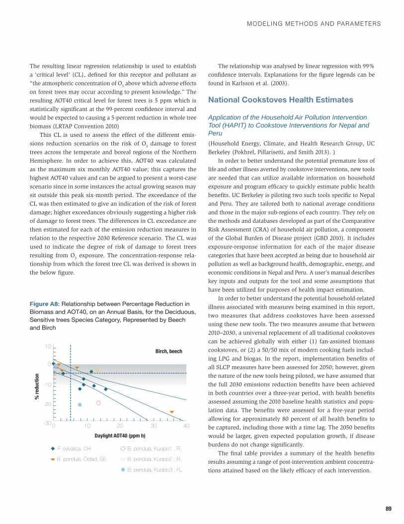
modelInG methods and Parameters
89
The resulting linear regression relationship is used to establish a ‘critical level’ (CL), defined for this receptor and pollutant as “the atmospheric concentration of O3 above which adverse effects on forest trees may occur according to present knowledge.” The resulting AOT40 critical level for forest trees is 5 ppm which is statistically significant at the 99-percent confidence interval and would be expected to causing a 5-percent reduction in whole tree biomass (LRTAP Convention 2010).
This CL is used to assess the effect of the different emis-sions reduction scenarios on the risk of O3 damage to forest trees across the temperate and boreal regions of the Northern Hemisphere. In order to achieve this, AOT40 was calculated as the maximum six monthly AOT40 value; this captures the highest AOT40 values and can be argued to present a worst-case scenario since in some instances the actual growing season may sit outside this peak six-month period. The exceedance of the CL was then estimated to give an indication of the risk of forest damage; higher exceedances obviously suggesting a higher risk of damage to forest trees. The differences in CL exceedance are then estimated for each of the emission reduction measures in relation to the respective 2030 Reference scenario. The CL was used to indicate the degree of risk of damage to forest trees resulting from O
3 exposure. The concentration-response rela-tionship from which the forest tree CL was derived is shown in the below figure.
The relationship was analysed by linear regression with 99% confidence intervals. Explanations for the figure legends can be found in Karlsson et al. (2003).
National Cookstoves Health Estimates
Application of the Household Air Pollution Intervention Tool (HAPIT) to Cookstove Interventions for Nepal and Peru(Household Energy, Climate, and Health Research Group, UC Berkeley (Pokhrel, Pillarisetti, and Smith 2013). )
In order to better understand the potential premature loss of life and other illness averted by cookstove interventions, new tools are needed that can utilize available information on household exposure and program efficacy to quickly estimate public health benefits. UC Berkeley is piloting two such tools specific to Nepal and Peru. They are tailored both to national average conditions and those in the major sub-regions of each country. They rely on the methods and databases developed as part of the Comparative Risk Assessment (CRA) of household air pollution, a component of the Global Burden of Disease project (GBD 2010). It includes exposure-response information for each of the major disease categories that have been accepted as being due to household air pollution as well as background health, demographic, energy, and economic conditions in Nepal and Peru. A user’s manual describes key inputs and outputs for the tool and some assumptions that have been utilized for purposes of health impact estimation.
In order to better understand the potential household-related illness associated with measures being examined in this report, two measures that address cookstoves have been assessed using these new tools. The two measures assume that between 2010–2030, a universal replacement of all traditional cookstoves can be achieved globally with either (1) fan-assisted biomass cookstoves, or (2) a 50/50 mix of modern cooking fuels includ-ing LPG and biogas. In the report, implementation benefits of all SLCP measures have been assessed for 2050; however, given the nature of the new tools being piloted, we have assumed that the full 2030 emissions reduction benefits have been achieved in both countries over a three-year period, with health benefits assessed assuming the 2010 baseline health statistics and popu-lation data. The benefits were assessed for a five-year period allowing for approximately 80 percent of all health benefits to be captured, including those with a time lag. The 2050 benefits would be larger, given expected population growth, if disease burdens do not change significantly.
The final table provides a summary of the health benefits results assuming a range of post-intervention ambient concentra-tions attained based on the likely efficacy of each intervention.
% re
duct
ion
10
-10
-20
-30
0
0 20 30 4010
F. sylvatica, CH
B. pendula, Ostad, SE
B. pendula, Kuopio1 , FL
B. pendula, Kuopio2 , FL
B. pendula, Kuopio3 , FL
Birch, beech
Daylight AOT40 (ppm h)
Figure A8: Relationship between Percentage Reduction in Biomass and AOT40, on an Annual Basis, for the Deciduous, Sensitive trees Species Category, Represented by Beech and Birch
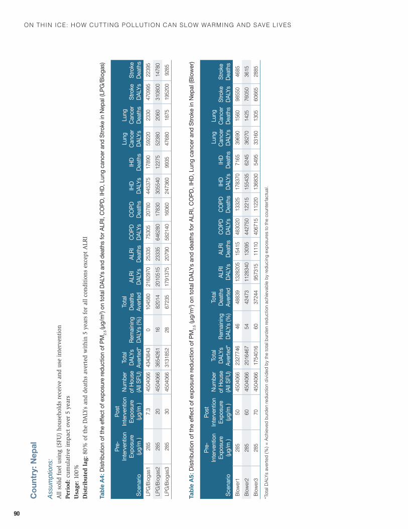
On thin ice: hOw cutting pOllutiOn can slOw warming and save lives
90
Co
untr
y: N
epal
Assu
mpt
ions
: A
ll so
lid f
uel u
sing
(SF
U)
hous
ehol
ds r
ecei
ve a
nd u
se in
terv
enti
onPe
riod
: cu
mul
ativ
e im
pact
ove
r 5
year
sU
sage
: 10
0%D
istr
ibu
ted
lag:
80%
of
the
DA
LYs
and
deat
hs a
vert
ed w
ithi
n 5
year
s fo
r al
l con
diti
ons
exce
pt A
LRI
Tabl
e A4
:Distrib
utionofth
eeff
ecto
fexposureredu
ctionofPM
2.5 (µg/m
3 ) on
tota
l DAL
Ys a
nd d
eath
s fo
r ALR
I, CO
PD, I
HD, L
ung
canc
er a
nd S
troke
in N
epal
(LPG
/Bio
gas)
Scen
ario
Pre-
In
terv
entio
n Ex
posu
re
(µg/m
3 )
Post
In
terv
entio
n Ex
posu
re
(µg/m
3 )
Num
ber
of H
ouse
(A
ll SFU
)
Tota
l DA
LYs
Aver
ted*
Rem
aining
DA
LYs (
%)
Tota
l De
aths
Av
erte
dAL
RI
DALY
sAL
RI
Deat
hsCO
PD
DALY
sCO
PD
Deat
hsIH
D DA
LYs
IHD
Deat
hs
Lung
Ca
ncer
DA
LYs
Lung
Ca
ncer
De
aths
Stro
ke
DALY
sSt
roke
De
aths
lPG
/Bio
gas1
285
7.3
4504
066
4343
843
010
4580
2182
970
2533
575
305
2078
044
5375
1789
059
220
2330
4709
9522
395
lPG
/Bio
gas2
285
2045
0406
636
5426
116
8201
420
1051
523
335
6462
8017
830
3055
4012
275
5238
020
6031
0800
1478
0lP
G/B
ioga
s328
530
4504
066
3131
852
2867
235
1791
375
2079
058
2140
1606
024
7360
9935
4768
018
7519
5200
9285
Tabl
e A5
:Distribu
tionofth
eeff
ecto
fexposureredu
ctionofPM
2.5(µg
/m3 )
on to
tal D
ALYs
and
dea
ths
for A
LRI,
CO
PD, I
HD,
Lun
g ca
ncer
and
Stro
ke in
Nep
al (B
low
er)
Scen
ario
Pre-
Inte
rven
tion
Expo
sure
(µg/m
3 )
Post
In
terv
entio
n Ex
posu
re
(µg/m
3 )
Num
ber
of H
ouse
(A
ll SFU
)
Tota
l DA
L Ys
Aver
ted*
Rem
aining
DA
LYs (
%)
Tota
l De
aths
Av
erte
dAL
RI
DALY
sAL
RI
Deat
hsCO
PD
DALY
sCO
PD
Deat
hsIH
D DA
LYs
IHD
Deat
hs
Lung
Ca
ncer
DA
LYs
Lung
Ca
ncer
De
aths
Stro
ke
DALY
sSt
roke
De
aths
Blow
er1
285
5045
0406
623
2774
646
4883
913
2820
515
415
4830
2013
325
1783
7071
6539
690
1560
9855
046
85Bl
ower
228
560
4504
066
2016
467
5442
473
1128
340
1309
544
2750
1221
515
5435
6245
3627
014
2576
050
3615
Blow
er3
285
7045
0406
617
5401
660
3724
495
7315
1111
040
6715
1122
013
6830
5495
3316
013
0560
665
2885
*Tot
al D
ALYs
ave
rted
(%) =
Ach
ieve
d bu
rden
redu
ctio
n di
vide
d by
the
tota
l bur
den
redu
ctio
n ac
hiev
able
by
redu
cing
exp
osur
es to
the
coun
terfa
ctua
l.
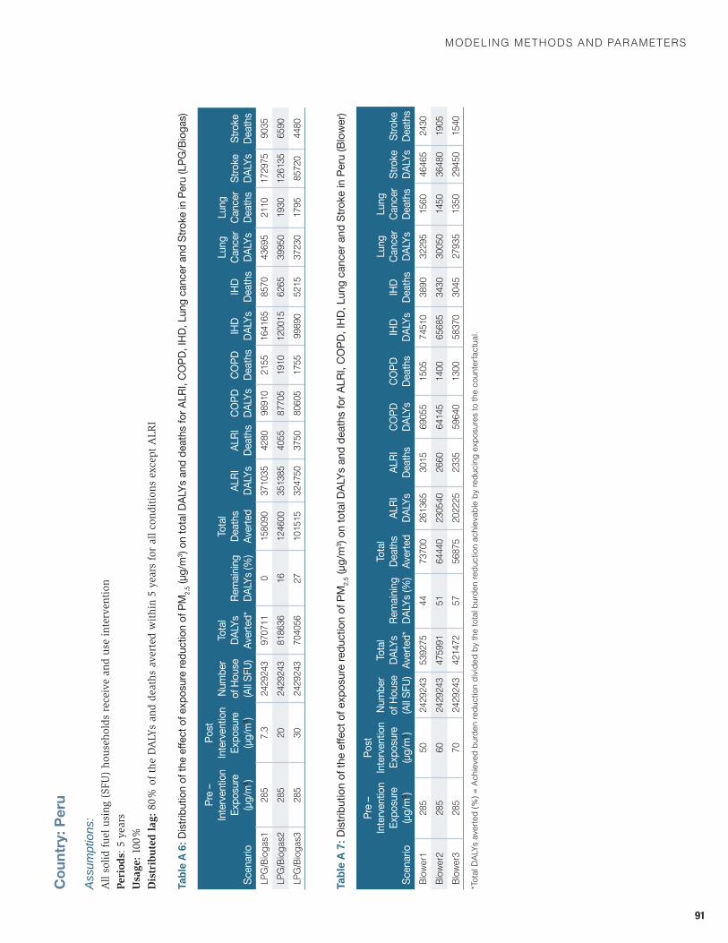
modelInG methods and Parameters
91
Co
untr
y: P
eru
Assu
mpt
ions
:A
ll so
lid f
uel u
sing
(SF
U)
hous
ehol
ds r
ecei
ve a
nd u
se in
terv
enti
onPe
riod
s: 5
yea
rsU
sage
: 10
0%D
istr
ibu
ted
lag:
80%
of
the
DA
LYs
and
deat
hs a
vert
ed w
ithi
n 5
year
s fo
r al
l con
diti
ons
exce
pt A
LRI
Tabl
e A
6:Distrib
utionofth
eeff
ecto
fexposureredu
ctionofPM
2.5(µg
/m3 )
on to
tal D
ALYs
and
dea
ths
for A
LRI,
COPD
, IHD
, Lun
g ca
ncer
and
Stro
ke in
Per
u (L
PG/B
ioga
s)
Scen
ario
Pre
–In
terv
entio
n Ex
posu
re
(µg/m
3 )
Post
In
terv
entio
n Ex
posu
re
(µg/m
3 )
Num
ber
of H
ouse
(A
ll SFU
)
Tota
l DA
LYs
Aver
ted*
Rem
aining
DA
LYs (
%)
Tota
l De
aths
Av
erte
dAL
RI
DALY
sAL
RI
Deat
hsCO
PD
DALY
sCO
PD
Deat
hsIH
D DA
LYs
IHD
Deat
hs
Lung
Ca
ncer
DA
LYs
Lung
Ca
ncer
De
aths
Stro
ke
DALY
sSt
roke
De
aths
lPG
/Bio
gas1
285
7.3
2429
243
9707
110
1580
9037
1035
4280
9891
021
5516
4165
8570
4369
521
1017
2975
9035
lPG
/Bio
gas2
285
2024
2924
381
8636
1612
4600
3513
8540
5587
705
1910
1200
1562
6539
950
1930
1261
3565
90lP
G/B
ioga
s328
530
2429
243
7040
5627
1015
1532
4750
3750
8060
517
5599
890
5215
3723
017
9585
720
4480
Tabl
e A
7:Distribu
tionofth
eeff
ecto
fexposureredu
ctionofPM
2.5(µg
/m3 )
on to
tal D
ALYs
and
dea
ths
for A
LRI,
CO
PD, I
HD,
Lun
g ca
ncer
and
Stro
ke in
Per
u (B
low
er)
Scen
ario
Pre
–In
terv
entio
n Ex
posu
re
(µg/m
3 )
Post
In
terv
entio
n Ex
posu
re
(µg/m
3 )
Num
ber
of H
ouse
(A
ll SFU
)
Tota
l DA
L Ys
Aver
ted*
Rem
aining
DA
LYs (
%)
Tota
l De
aths
Av
erte
dAL
RI
DALY
sAL
RI
Deat
hsCO
PD
DALY
sCO
PD
Deat
hsIH
D DA
LYs
IHD
Deat
hs
Lung
Ca
ncer
DA
LYs
Lung
Ca
ncer
De
aths
Stro
ke
DALY
sSt
roke
De
aths
Blow
er1
285
5024
2924
353
9275
4473
700
2613
6530
1569
055
1505
7451
038
9032
295
1560
4646
524
30Bl
ower
228
560
2429
243
4759
9151
6444
023
0540
2660
6414
514
0065
685
3430
3005
014
5036
480
1905
Blow
er3
285
7024
2924
342
1472
5756
875
2022
2523
3559
640
1300
5837
030
4527
935
1350
2945
015
40
*Tot
al D
ALYs
ave
rted
(%) =
Ach
ieve
d bu
rden
redu
ctio
n di
vide
d by
the
tota
l bur
den
redu
ctio
n ac
hiev
able
by
redu
cing
exp
osur
es to
the
coun
terfa
ctua
l.

On thin ice: hOw cutting pOllutiOn can slOw warming and save lives
92
Endnotes1 http://www.globalfiredata.org/Data/index.html,2 Environmental Benefits Mapping and Analysis Program (BenMAP). Information is available online at: http://www.epa.gov/air/benmap3 Modifications include merging Norfolk Island with Australia, merging Svalbard with Norway, and combining Guernsey and Jersey into the Channel Islands. This was done to match UN definitions of the areas.4 http://www.healthmetricsandevaluation.org/sites/default/files/publication_summary/.

the world bank1818 H Street, NWWashington, DC 20433
www.worldbank.org
Top Related