


Languages
Pages
Legal

PROSPECTS OF RENEWABLE AND NON-RENEWABLE
ENERGY SOURCES IN SOUTH ASIAN ECONOMIES: AN
ANALYSIS
BY
SADIA ALI
Registration No: 2013-GCUF-05034
Thesis submitted in partial fulfillment of
the requirement for the degree of
DOCTOR OF PHILOSOPHY
IN
ECONOMICS
DEPARTMENT OF ECONOMICS
GOVERNMENT COLLEGE UNIVERSITY FAISALABAD
2017

ii
CERTIFICATE OF APPROVAL
This is to certify that the research work presented in this thesis, entitled, “Prospects of
Renewable and Non-Renewable Energy Sources in South Asian Economies: An Analysis”
was conducted by Mrs. Sadia Ali (Regd. No 2013-GCUF-05034) under the supervision of Dr.
Sofia Anwar.

iii
CERTIFICATE BY SUPERVISORY COMMITTEE
We certify that the contents and form of a thesis submitted by Miss Sadia Ali,
registration No. 2013-GCUF-05034 has been found satisfactory and in accordance with
the prescribed format. We recommend it to be processed for the evaluation by the
External Examiner for the award of the degree.
Supervisor
Co-Supervisor
Member of Supervisory Committee
Chairperson
Dean / Academic Coordinator

iv
AUTHORS DECLARATION
I Sadia Ali, Reg. No 2013-GCUF-05034, here by state that my Ph.D. thesis title
“Prospects of Renewable and Non-Renewable Energy Sources in South Asian
Economies: An Analysis” is my own work and has not been submitted previously by
me for taking any degree from Government College University, Faisalabad or anywhere
else in the country/ world. At any time if my statement is found to be incorrect even
after my graduate the university has the right to withdraw my Ph.D. degree.

v
PLAGIARISM UNDERTAKING
I solemnly declare that research work presented in the thesis titled “Prospects of
Renewable and Non-Renewable Energy Sources in South Asian Economies: An Analysis”
is solely my research work with no significant contribution from any other person. Small
contribution/help wherever taken has bees been duly acknowledged and that complete thesis
has been written by me.
I understand the zero-tolerance policy of the HEC and Government College University,
Faisalabad towards plagiarism. Therefore, as an author of the above titled thesis declare that no
portion of my thesis has been plagiarized and any material used as reference is properly
referred/cited.
I undertake that if l am found guilty of any formal plagiarism in the above titled thesis
even after award of Ph.D. degree, the University reserve the rights to withdraw/revoke my Ph.D.
degree and that HEC and the University has the right to publish my name on the
HBC/University Website on which names of students are placed who submitted plagiarized
thesis.

vi
DEDICATION
Dedicated to
“My Parents”
For Their Love, Encouragement and Prayers
“Muhammad Amir Javed”
For His Support and Believe in Richness of Learning
“Muhammad Husnain Amir, Muhammad Ali Amir and Zainab Amir”
For Their Love, Prayers and Made Me Keen for Learning

vii
ACKNOWLEDGEMENTS
First of all, I would praise the Almighty Allah, the Gracious and the Most Merciful, for
giving me the quality and inspiration to complete this examination.
I might want to thank my Supervisor, Dr. Sofia Anwar not just for her few astute
remarks concerning the bearing and the substance of this proposition, yet in addition
for her human state of mind and for being understanding. She prepared me how to make
inquiries and express my thoughts. She indicated me diverse approaches to approach
an exploration issue and the need to steady keeping in mind the end goal to achieve any
objective. She showed me how to buckle down. I sincerely value the time she has
committed to regulate my exploration.
I might want to formally recognize and thank various individuals, particularly my co-
supervisor, Dr. Samia Nasreen who empowered, supported and helped me through the
testing a very long time of my Ph. D examinations. Thanks to Dr. Muhammad Rizwan
Yasin for agreeing to serve on my committee. I am also thankful to Dr Muhammad
Sohail Amjad Makhdom for his encouragement and support during my PhD.
Last, yet not slightest, I thank my family: my parents, for giving me life in the first
place, for instructing, educating, support and consolation to seek my interests. My
husband, my siblings for tuning in to my protests and dissatisfactions, and for having
faith in me.
SADIA ALI
viii
TABLE OF CONTENTS
CERTIFICATE OF APPROVAL…………………………………………ii
CERTIFICATE BY SUPERVISORY COMMITTEE………………………..….......iii
AUTHORS DECLARATION…………………………………………....…………..iv
PLAGIARISM UNDERTAKING…………………….…………………………........v
DEDICATION………………………………………………………………………..vi
ACKNOWLEDGEMENTS…………………………………………………....….…vii
ACRONYMS AND ABREVIATIONS……………….…………………………....xxii
ABSTRACT………………………………………………………………………..xxiii
1. INTRODUCTION……………………….………………………………….………1
1.1 Research Motivation…………………………………………………………..…...8
1.2 Research objectives………………………………………………………….……..9
1.3 Research Contribution………………………………………………………..…..10
1.4 Research Structure………….…………………………………………………….10
2. REVIEW OF LITERATURE………………………..…………………………….12
2.1 Empirical Literature.........................................................................................…...12
2.1.1 Renewable and nonrenewable energy and economic growth..…………………11
2.1.2 Renewable and nonrenewable energy consumption and environment
quality…………………………………………………………………………...……30
2.1.3 Demand for Renewable and nonrenewable energy…….…………...…………..38
2.1.4 Renewable and Non-Renewable Energy Sources, Energy Intensity, Economic
Growth………………………………………………………………………………..47
2.2 Theoretical Literature………………………………………………….…………51
2.2.1 Prospects and Potential of Renewable and Non-Renewable Energy
Sources………………………………………….……………………..…….…….....51
3. METHODOLOGY....…………..……………………………………………...71
ix
3.1 Data……………………………………………………………………….………71
3.2 Model Specification……………………………………………………………....71
3.2.1 Renewable and nonrenewable energy with growth……..…..…………………..72
3.2.1.1 Model 1. Relationship between Renewable and Non-renewable Energy,
Institutions and Economic Growth …………………………………………..………72
3.2.1.2 Model 2: Relationship between Renewable and Non-renewable Energy,
Urbanization and Economic Growth…………..…………………………..………….73
3.2.1.3 Model 3: Relationship between Renewable and Non-renewable Energy,
Financial Development and Economic Growth ………………...….………………....74
3.2.1.4 Data Sources…...…………...….…………………………………..…………75
3.2.2 Renewable and nonrenewable energy with Environment Quality…….….……..75
3.2.2.1 Model 4: Relationship between Renewable and Non-renewable Energy,
Population Density and Environment ………………………..……………...………..75
3.2.2.2 Model 5: Relationship between Renewable and Non-renewable Energy,
Urbanization, Energy Intensity and Environment …….…………………..….……....76
3.2.2.3 Data Sources……………………………………………………………….…78
3.2.3 Demand Elasticity of Renewable and nonrenewable energy…………...………78
3.2.3.1 Model 6: Relationship between Renewable Energy Demand, Economic Growth,
Industrialization, Technological Changes and Energy Price ………………..……….78
3.2.3.2 Model 7: Relationship between Non-Renewable Energy Demand, Economic
Growth, Industrialization, Technological Changes and Energy Price …………….…79
3.2.3.3 Data Sources…………………………………………………………….……81
3.2.4 Renewable and nonrenewable energy with energy Efficiency……………….…81
3.2.4.1 Model 8: Relationship between Renewable and Non-renewable Energy,
Economic Growth, Urbanization and Energy Intensity ………………...…….………82
3.2.4.2 Model 9: Relationship between Renewable and Non-renewable Energy,
Economic Growth, Trade Openness and Energy Intensity ……………...……………82
3.2.4.3 Model 10: Relationship between Renewable and Non-renewable Energy,
Economic Growth, Industrialization, Technological Progress and Energy Intensity....82
3.2.4.4 Data Sources………………………………………………………………….83
x
3.3 Econometrics Methodology……………...…………………………………….…84
3.3.1 Time-Series Methodology………………..………………………………….....84
3.3.1.1 Unit Root Tests…………….…………………………………………………84
3.3.1.2 Johansen Co-integration Test ……………………………………………..….85
3.3.2 Panel Data Methodology…………………………………………...…………...88
3.3.2.1 Panel Unit Root Tests………………………………………………………....88
3.3.2.1.1 LLC Unit Root Test…….………………………..………………...………..88
3.3.2.1.2 IPS Unit Root Test………………………..………………………………...90
3.3.2.2 Panel Co-integration Test…………………………………………..…………91
3.3.2.2.1 Estimation of Panel Co-integration Regression……….……………...…….93
3.3.3 Panel Granger Causality Test …………………………………………………..94
4. RESULTS AND DISCUSSIONS……………………….…………………………96
4.1 An Overview of South Asian Economies…….…….………….…………...…….96
4.1.1 Economic Structure………………..…………………………………………...96
4.1.1.1 Economic Growth………………..……………………………………...……96
4.1.1.2 Inflation………...………………..……………………………………...……97
4.1.1.3 Industrial Share …………..……..………………………….…………...……98
4.1.2 Population Desity ….……………...………………………….…………...……99
4.1.3 Environment………………..……..……………………….…………….....…100
4.2 Energy Situation In South Asia ………………..………….………………….…101
4.3 Importance and Potential of Renewable Energy Sources ……………............…105
xi
4.4 Empirical results and discussions……………………………………………..…108
4.4.1 Impact of renewable and nonrenewable energy on economic growth……....…108
4.4.1.1 Model 1: Relationship between Renewable and Non-renewable Energy,
Institutions and Economic Growth ………..……………………………..…….….108
4.4.1.1.1. Time Series Results…………………………………….……...................108
4.4.1.1.1.1. Unit Root Test Results………………………..…..……………….…...108
4.4.1.1.1.2. Johansen Co-integration Test Results…………………………..……....110
4.4.1.1.2 Panel Results…………………………………………………………....…111
4.4.1.1.2.1 Panel Unit Root Results………………………………………..….…….112
4.4.1.1.2.2 Panel Co-integration Results………………………...…………………..113
4.4.1.1.3 FMOLS Estimates……………...…………………………...…..…………113
4.4.1.1.3.1 FMOLS Estimates Country Wise…………………………….…………113
4.4.1.1.3.2 FMOLS Panel Estimates……………………….……………………..…115
4.4.1.1.4 Panel Causality Results…………...…………………………………...…..116
4.4.1.2 Model 2: Relationship between Renewable and Non-renewable Energy,
Urbanization and Economic Growth ……………………………………………..…117
4.4.1.2.1 Time Series Results……………………………………………………..…117
4.4.1.2.1.1 Unit Root Test Results……………………………...……………..…….117
4.4.1.2.1.2 Johansen Co-integration Test Results………………………....………...118
4.4.1.2.2 Panel Results………………………...…………………..……………...…120
4.4.1.2.2.1 Panel Unit Root Results ……………………………..…..………….…..120
4.4.1.2.2.2 Panel Co-integration Results…………………………..…..…………….121
4.4.1.2.3 FMOLS Estimates……………………………...………………………….122
4.4.1.2.3.1 FMOLS Estimates Country Wise……………………………….………122
4.4.1.2.3.2 FMOLS Panel Estimates………………………………………...………123
xii
4.4.1.2.4 Panel Causality Results……………………………………………..……..124
4.4.1.3 Model 3: Relationship between Renewable and Non-renewable Energy,
Financial Development and Economic Growth ………….…….………………..….125
4.4.1.3.1 Time Series Results………..…….………………….…………………..…125
4.4.1.3.1.1 Unit Root Test Results……………………………….…...…………..…125
4.4.1.3.1.2 Johansen Co-integration Test Results…………....………………...……126
4.4.1.3.2 Panel Results……………………………………………...……….……...128
4.4.1.3.2.1 Panel Unit Root Results………….………………………………...……128
4.4.1.3.2.2 Panel Co-integration Results………………………………………….....129
4.4.1.3.3 FMOLS Estimates……………………………………………………...….130
4.4.1.3.3.1 FMOLS Estimates Country Wise………..………………………………130
4.4.1.3.3.2 FMOLS Panel Estimates………………………………………………...131
4.4.1.3.4 Panel Causality Results……………………………………………………132
4.4.2. Impact of Renewable and Non-Renewable Energy Sources on Environmental
Quality………………………………………………………………………...…….133
4.4.2.1 Model 4: Relationship between Renewable and Non-renewable Energy,
Population Density and Environment ………………………………………………133
4.4.2.1.1 Time Series Results………………………………..………………………133
4.4.2.1.1.1 Unit Root Test Results…………………….…..……………………..….133
4.4.2.1.1.2 Johansen Co-integration Test Results……..…...…………...…………...135
4.4.2.1.2 Panel Results…………………………………….……………………...…137
4.4.2.1.2.1 Panel Unit Root Results…………………………………………………137
4.4.2.1.2.2 Panel Co-integration Results………...………………………………..…138
4.4.2.1.3 FMOLS Estimates…………………..………………………………..……139
4.4.2.1.3.1 FMOLS Estimates Country Wise……………………………………..…139
4.4.2.1.3.2 FMOLS Panel Estimates……...……..………………………………..…140
4.4.2.1.3.4 Panel Causality Results………………………………………….………142
xiii
4.4.2.2 Model 5: Relationship between Renewable and Non-renewable Energy,
Urbanization, Energy Intensity and Environment…..………………………...…….143
4.4.2.2.1 Time Series Results………………………………..………………………143
4.4.2.2.1.1 Unit Root Test Results…………………….…..……………………..….143
4.4.2.2.1.2 Johansen Co-integration Test Results……..…...…………...…………...145
4.4.2.2.2 Panel Results…………………………………….……………………...…147
4.4.2.2.2.1 Panel Unit Root Results…………………………………………………147
4.4.2.2.2.2 Panel Co-integration Results………...………………………………..…148
4.4.2.2.3 FMOLS Estimates…………………..………………………………..……149
4.4.2.2.3.1 FMOLS Estimates Country Wise……………………………………..…149
4.4.2.2.3.2 FMOLS Panel Estimates……...……..…………………………………..151
4.4.2.2.3.4 Panel Causality Results………………………………………….………152
4.4.3 Demand for Renewable and Non-Renewable Energy Sources…………...……153
4.4.3.1 Model 6: Demand for Renewable Energy Sources……………………….….153
4.4.3.1.1 Time Series Results…………………………………………………….….153
4.4.3.1.1.1 Unit Root Test Results……………………………………………...…...153
4.4.3.1.1.2 Johansen Co-integration Test Results………………………………...…158
4.4.3.1.2 Panel Results……...…………………………………….…………………156
4.4.3.1.2.1 Panel Unit Root Results…………..…………………………..…...…….156
4.4.3.1.2.2 Panel Co-integration Results……………………………………..……...158
4.4.3.1.3 FMOLS Estimates……………………………………………………...….158
4.4.3.1.3.1 FMOLS Estimates Country Wise………………………………..………158
4.4.3.1.3.2 FMOLS Panel Estimates………………………………………………...160
4.4.3.1.4 Panel Causality Results……………………………………………………161
4.4.3.1.5 Test of Forecasting Renewable Energy Demand…………………………162
4.4.3.1.5.1 Variance Decomposition of RE Demand…...………………...…….…...162
xiv
4.4.3.1.5.2 Impulse Response Function of RE Demand…………………………......162
4.4.3.2. Model 7: Demand for Non-Renewable Energy Sources…………...………..162
4.4.3.2.1 Time Series Results…….………………….………………………………162
4.4.3.2.1.1 Unit Root Test Results……………………………………………….….162
4.4.3.2.1.2 Johansen Co-integration Test Results…………………………………...164
4.4.3.2.2 Panel Results..……………………………………………………………..166
4.4.3.2.2.1 Panel Unit Root Results…………………………………………………166
4.4.3.2.2.2 Panel Co-integration Results…………………………………………….167
4.4.3.2.3 FMOLS Estimates……………………………………………….………...167
4.4.3.2.3.1 FMOLS Estimates Country Wise………………………………….…….167
4.4.3.2.3.2 FMOLS Panel Estimates…………………………………………….…..169
4.4.3.2.4 Panel Causality Results………………………………………………....…170
4.4.3.2.5 Test of Forecasting Non-Renewable Energy Demand……………………171
4.4.3.2.5.1 Variance Decomposition of NRE Demand……………………………...171
4.4.3.2.5.2 Impulse Response Function of NRE Demand…………………………...171
4.4.4. Impact of Renewable and Non-Renewable Energy Sources on Energy
Intensity……………………………………………………………………..171
4.4.4.1 Model 8: Relationship between Renewable and Non-renewable Energy,
Economic Growth, Urbanization and Energy Intensity ………………..……171
4.4.4.1.1 Time Series Results……….………………………………………….……171
4.4.4.1.1.1 Unit Root Test Results….…………………………………………...…..171
4.4.4.1.1.2 Johansen Co-integration Test Results………………………………...…173
4.4.4.1.2 Panel Results………………………………………………………………175
4.4.4.1.2.1 Panel Unit Root Results………………………………………………....175
4.4.4.1.2.2 Panel Co-integration Results…………………………………………….176
4.4.4.1.3 FMOLS Estimates…………………………………………..……..………177
xv
4.4.4.1.3.1 FMOLS Estimates Country Wise……………………………....………..177
4.4.4.1.3.2 FMOLS Panel Estimates…………………………………….……..……178
4.4.4.1.4 Panel Causality Results……………………………………….………...…179
4.4.4.2 Model 9: Relationship between Renewable and Non-renewable Energy,
Economic Growth, Trade Openness and Energy Intensity ………………………….180
4.4.4.2.1 Time Series Results………………………………………….…………….180
4.4.4.2.1.1 Unit Root Test Results…………………………………………………..180
4.4.4.2.1.2 Johansen Co-integration Test Results……………….…………………..182
4.4.4.2.2 Panel Results………………………………………………………………183
4.4.4.2.2.1 Panel Unit Root Results……………………………………………...….183
4.4.4.2.2.2 Panel Co-integration Results…………………………………………….185
4.4.4.2.3 FMOLS Estimates……………………………………….…...……………185
4.4.4.2.3.1 FMOLS Estimates Country Wise……………………………………..…185
4.4.4.2.3.2 FMOLS Panel Estimates……………………………………….………..187
4.4.4.2.4 Panel Causality Results…………………...………………………...……..188
4.4.4.3. Model 10: Relationship between Renewable and Non-renewable Energy,
Economic Growth, Industrialization, Technological Progress and Energy Intensity
………………………………………………………………………………….…...189
4.4.4.3.1. Time Series Results……………………………………………………….189
4.4.4.3.1.1. Unit Root Test Results……………………………………….…………189
4.4.4.3.1.2. Johansen Co-integration Test Results…………………………………..191
4.4.4.3.2 Panel Results …………………………………………………………..….192
4.4.4.3.2.1 Panel Unit Root Results………………………………………………....192
4.4.4.3.2.2 Panel Co-integration Results………………………………...…………..194
4.4.4.3.3 FMOLS Estimates…………………………………………………………195
4.4.4.3.3.1 FMOLS Estimates Country Wise……………….………………...…..…195
xvi
4.4.4.3.3.2 FMOLS Panel Estimates…………………………………………..…….196
4.4.4.3.4 Panel Causality Results……………………………………………….…...197
5. CONCLUSIONS AND RECOMENDATIONS…………………………….....…199
5.1 Summary and Conclusion…….……………………………………………...….199
5.2 Policy recommendation...………………………………………………….........202
REFRENCES……………………………………………………………………….204
Appendices ………………………………………………………………………....238
xvii
LIST OF TABLES
Table 2.1. Summary of Empirical studies……………………………………………65
Table 4.1 Energy Dependence of Selected South Asian Countries………………….102
Table 4.2 Production and Use of Energy ……………………………………………102
Table 4.3 Non-renewable Energy Sources (oil)……………………………..………103
Table 4.4 Non-renewable Energy Sources (Gas)……………..………………….....103
Table 4.5 Non-renewable Energy Sources (Coal)…………………………..………104
Table 4.6 Renewable Energy Sources (Hydro)………………………………...……104
Table 4.7 Renewable Energy Sources……………………………………………….104
Table 4.8 Importance of Renewable and Non-renewable energy sources……..……105
Table 4.9 Renewable Energy potential………………………………………………107
Table 4.10 DF GLS Unit root Test……………..…….……………………...…..….109
Table 4.11 Johansen Co-integration Test results.....………………………...……….110
Table 4.12 Panel Unit root Test…..……………………………………….....………112
Table 4.13 Panel co-integration Test …………………………..………...….………113
Table 4.14 FMOLS Country Specific Results…………...………………,………….114
Table 4.15 FMOLS Panel Estimates………………………...………...…….………116
Table 4.16 DH panel causality Test …………………………………..……..………116
Table 4.17 DF GLS Unit root Test …………………………….…..……………......117
Table 4.18 Johansen Co-integration Test results……………..…..…………………119
Table 4.19 Panel Unit root Test…..…………………………..……..………………120
Table 4.20 Panel Co-integration Test ……………………………...………………..121
Table 4.21 FMOLS Country Specific Results…………………….…………………122
Table 4.22 FMOLS Panel Estimates……………………………...…………………124
xviii
Table 4.23 DH Panel Causality Test ………………………….……………………..124
Table 4.24 DF GLS Unit root Test…………………...……………………………..125
Table 4.25 Johansen Co-integration Test results.…………………………...……….127
Table 4.26 Panel Unit root Test……………………..……………………..……..…128
Table 4.27 Panel co-integration Test …………………….…………….………...…129
Table 4.28 FMOLS Country Specific Results………………………………….…...130
Table 4.29 FMOLS Panel Estimates…………………………………….……….….132
Table 4.30 DH panel causality Test ……………………………….……..……….…133
Table 4.31 DF GLS Unit root Test …………………………………………..….......134
Table 4.32 Johansen Co-integration Test results…………………….………..….…135
Table 4.33 Panel Unit root Test…………………………………………..…………137
Table 4.34 Panel Co-integration Test …………………..…………………………..138
Table 4.35 FMOLS Country Specific Results………………………………………139
Table 4.36 FMOLS Panel Estimates……………………………………..…….……141
Table 4.37: FMOLS Country Specific Results ……………………………………...142
Table 4.38 DF GLS Unit root Test…………………...………………………….….143
Table 4.39 Johansen Co-integration Test results.…………………………...………145
Table 4.40 Panel Unit root Test……………………..……………………..………..147
Table 4.41 Panel co-integration Test ………………...………………….………..…148
Table 4.42 FMOLS Country Specific Results……………………………………....149
Table 4.43 FMOLS Panel Estimates……………………………………..…….……151
Table 4.44 DH panel causality Test …………………………..…………..…….…...152
Table 4.45 DF GLS Unit root Test…………………...………………….……….….153
Table 4.46 Johansen Co-integration Test results.…………………………...………155
xix
Table 4.47 Panel Unit root Test……………………..……………………..………..157
Table 4.48 Panel co-integration Test …………………..……………….………..…158
Table 4.49 FMOLS Country Specific Results……………………………………....159
Table 4.50 FMOLS Panel Estimates…………………………………….……..……160
Table 4.51 DH panel causality Test ……………………………………..……..…...161
Table 4.52 DF GLS Unit root Test…………………...………………….……….….163
Table 4.53 Johansen Co-integration Test results.…………………………...………164
Table 4.54 Panel Unit root Test……………………..……………………..…….…..166
Table 4.55 Panel co-integration Test ………………..………………….………...…167
Table 4.56 FMOLS Country Specific Results…………………………………….....168
Table 4.57 FMOLS Panel Estimates…………………………………….…….….…169
Table 4.58 DH panel causality Test ……………………………………..…….…....170
Table 4.59 DF GLS Unit root Test…………………...………………….….………172
Table 4.60 Johansen Co-integration Test results.…………………………...……….173
Table 4.61 Panel Unit root Test……………………..……………………..………..175
Table 4.62 Panel co-integration Test ……………………….………….….…….….176
Table 4.63 FMOLS Country Specific Results……………………………………....177
Table 4.64 FMOLS Panel Estimates…………………………………….…….……179
Table 4.65 DH panel causality Test ……………………………………..…….….....179
Table 4.66 DF GLS Unit root Test…………………...………………….………….180
Table 4.67 Johansen Co-integration Test results.…………………………...………182
Table 4.68 Panel Unit root Test……………………..……………………..………..184
Table 4.69 Panel co-integration Test …………………………….…….…..…….…185
Table 4.70 FMOLS Country Specific Results……………………………….……....186
xx
Table 4.71 FMOLS Panel Estimates…………………………………….…….……187
Table 4.72 DH panel causality Test ……………………………………..……...…...188
Table 4.73 DF GLS Unit root Test…………………...………………….…….…….189
Table 4.74 Johansen Co-integration Test results.…………………………...….……191
Table 4.75 Panel Unit root Test……………………..……………………..………..193
Table 4.76 Panel co-integration Test ………………………….……….……...….…194
Table 4.77 FMOLS Country Specific Results………………………………….…....195
Table 4.78 FMOLS Panel Estimates…………………………………….……..……197
Table 4.79 DH panel causality Test ……………………………………..……..…...198
Table A1 Variable Description ………………………………………….……..……238
Table B1 Summary Statistics of the variables Panel data 1980-2014………………240
Table B2 Summary Statistics of the variables Time Series data 1980-2014….…….241
Table C1 Variance Decomposition of RE Demand…………………………………244
Table C2 Impulse Response Function of RE Demand………………………………245
Table C3 Variance Decomposition of NRE Demand……………….……………….246
Table C4 Impulse Response Function of NRE Demand……………………………..247
xxi
LIST OF FIGURES
Figure 4.1: Trends in Economic Growth.…….………………………………...……..97
Figure 4.2: Trends in Inflation ……………….………………….………...………….98
Figure 4.3: Trends in Industrial share of GDP……………...….…………..………….98
Figure 4.4: Trends in Total Population ………………….…….…………..………….99
Figure 4.5: Trends Population Density………………….…….…………..………….99
Figure 4.6: Trends in per capita Co2 ………………………….…………...….……100
Figure 4.7: Trends in Non-Renewable energy Sources…………………….…….…101
Figure 4.8: Trends in Renewable energy Sources…………………………..………102
xxii
ACRONYMS AND ABBREVIATIONS
DF Dickey-Fuller
ECM Error Correction Mechanism
EC Energy Consumption
FBR Federal Board of Revenue
EI Energy Intensity
EFI Energy Efficiency
EKC Environment Kuznets Curve
FY Financial Year
GDP Gross Domestic Product
GLS Generalized Least Square
IEA Information Energy Authority
IND Industrialization
OLS Ordinary Least Squares
INS Institutions
FMOLS Fully Modified Ordinary Least Square
NRE Nonrenewable Energy
PD Population Density
RE Renewable Energy
TO Trade Openness
URB Urbanization
WDI World Bank Indicator
xxiii
ABSTRACT
The core target of this exploration is to inspect the effect of renewable and
nonrenewable energy sources on economic growth and environmental degradation in
selected South Asian Economies. The thesis explores renewable and non-renewable
energy sources in four ways. Firstly, it empirically investigates the relationship between
renewable, non-renewable energy, and economic growth. Secondly, it empirically
investigates the impact of renewable and non-renewable energy sources on
environmental quality. Thirdly, it examines the determinants of demand for renewable
and non-renewable energy sources including industrial sector. Fourthly, the study
explores the impact of aforementioned energy sources and economic growth on energy
intensity. The thesis comprises on four South Asian countries: Pakistan, India,
Bangladesh and Sri Lanka for empirical investigation, based on the availability of data.
The study employs both time series and panel data analysis for the period of 1980 to
2014. To analyze the long run and causal relationship between variables, we have
applied Johansson co-integration, Larsson panel co-integration and Granger causality
Dumitrescu and Hurlin (DH) approaches. Empirical results confirm the presence of
long run co-integration between economic growth, renewable energy sources, non-
renewable energy sources, institution quality, population density, financial
development, inflation, and trade openness in various models. The impact of renewable
and non-renewable energy on economic growth is found positive which increases per
capita GDP. The analysis of fully modified ordinary least squares (FMOLS) panel
estimates shows that the values of all coefficients are statistically significant and their
signs are in line with the economic growth theory.
Secondly, the results reveal that economic growth, population density, and non-
renewable energy have a positive impact on per capita CO2 emission. However, the
negative sign of renewable energy sources tends to decrease per capita CO2 emissions,
indicating that environmental quality deteriorates with non-renewable energy sources
and improves in case of renewable energy sources. The findings additionally encourage
the Environmental Kuznets Curve (EKC) hypothesis which accepts an altered U-shaped
path amongst affluence and per capita CO2 emissions. Moreover, the study found the
evidence of bi-directional panel causality between CO2 and renewable energy sources
as well as population destiny. Investigations give the evidence of unidirectional
xxiv
causality running from CO2 to non-renewable energy sources. Results also give proof
evidence of feedback relationship between environment and both energy sources.
In the other model of the causal relationship between environmental quality and energy
intensity with the presence of urbanization with both energy sources and population,
outcomes affirm the existence of co-integration between these factors. FMOLS
discovered the positive effect of affluence, urbanization, energy intensity and non-
renewable energy sources on CO2 emissions. Notwithstanding, the negative indication
of renewable energy sources demonstrate that it will prompt diminishing per capita
CO2.
Thirdly, the empirical analysis of renewable and non-renewable energy demand shows
that the price and income are the major determinants of the demand for energy. The
impact of income on energy demand is positive in both energy sources whereas, in case
of price, it has a negative impact. The results of technological progress show a negative
impact on energy demand, which suggests that technological progress is energy saving.
Results of FMOLS indicate that increase in economic growth, industrialization and
population total increases energy demand (renewable and non-renewable). These
results show that higher per capita real income should result in greater economic
activity which in turns accelerate the use of energy. The degree of industrialization, as
a measure of economic structure, is also expected to enhance the demand for renewable
energy. However, the negative sign of P and T indicates that increase in energy price
and technical progress will lead to decrease energy demand. The negative sign of
technical progress shows that the technology is energy saving.
Lastly, the impact of economic growth, population density and renewable energy on
energy intensity is found negative, which suggests that there is a reduction in energy
intensity with the increase in aforesaid factors. On the other hand, reduction in energy
intensity leads to the improvements in energy efficiency. Results of panel FMOLS
indicate that 1 percent increase in economic growth, renewable energy sources, and
population density decrease the energy intensity by about 0.600 percent, 0.027 percent
and 0.960 percent respectively which leads to increase in energy efficiency. Moreover,
the study found the evidence of bi-directional panel causality between energy intensity
and economic growth, urbanization as well as between energy intensity and population
density. Results provide evidence of feedback relationship between energy efficiency

xxv
and output. There is also unidirectional causality running from energy intensity to
renewable and non-renewable energy sources.
Keywords: Economic Growth, Environmental quality, Renewable energy, Non-
renewable Energy, Institutional quality, Industrialization, Energy Demand, Energy
Price, Population Density, South Asia
1
CHAPTER 1
INTRODUCTION
Energy is a fundamental component of human needs. Although it is not viewed as
compulsory requirement but is essential for the fulfillment of daily human needs (Yuko,
2004). Due to the rapid progress and industrialization improvements, the level and
power of energy utilization is essential for a nation's economic development. The
fundamental sources of energy are separated into two vital categories that is traditional
and maintainable energy sources. Traditional sources can be classified as energy from
non-renewable assets. These sources have various difficulties that include
contamination and an unnatural weather change; this has rolled out nation’s
improvement strategies to support reception of greener innovations in renewable power
sources. Renewable or maintainable energy sources are characterized as energy that can
be accomplished from assets which are actually renewed on a human extent, for
example daylight, biogas, wind, hydropower, tides, waves and geothermal warmth.
Renewable energy sources can be substituted regular or traditional sources in four
recognizable zones: power era, high temp water/space warming, engine fills, and
countryside (off-network) energy administrations. Petroleum product from fossil fuel
which incorporates coal, oil and flammable gas drove world economic development,
however this energizes arrival of carbon dioxide CO2 into the earth air, is viewed as
the fundamental driver of a dangerous atmospheric deviation and environmental change
(Stern, 2006). Renewable sources such as solar, wind, geothermal, tidal, and biomass
have an unlimited supply and these are being recycled or replaced. While energy
coming from fossil fuels, coal, oil and natural gas are non-renewable sources of energy
which is exhaustible up to a limit . We cannot enjoy the benefits of these non-renewable
energy sources forever, because they become unavailable once exhausted or in other
words these are one time use resources. Even the over-consumption of such sources can
leads to its threshold level, from where they cannot be regenerated for centuries.
Energy can be used for illumination, lighting, warming, and cookery on the one hand
and also as a medium of transportation on the other hand. Energy is required for
manufacturing consumer goods as well as capital equipment both in household and
production sectors. Globally, the demand for energy is increasing day by day. The
reasons are multiple, for instance, shift to industrialization, the introduction of new
2
technology, modernization and most importantly the desire for having a more
comfortable standard of living.
Energy is measured as an essential source for the socio-economic development of a
country whether it is renewable energy or non-renewable energy. Thus, each and every
sector of the economy has shared involvement of energy like in agriculture, industry,
transportation, social and public sector, household and business sector or trade, the use
of energy has become inevitable. Most of the developing and underdeveloped nations
are facing the issue of shortage of energy relative to its needs. (Chaudhry et al., 2015).
Traditional sources such as oil, natural gas, coal and electricity from oil are the most
important sources of energy and this energy supply approximately 90 percent of total
energy requirements at world level (Riaz, 1984). The sharp increase in oil prices and a
shortage of energy creates barriers to bring the rapid growth of the economy (Chaudhry
et al., 2015).
Economic growth of a country is denoted by the gain in Gross Domestic Product (GDP)
or the value of country’s output. On the other hand, economic development of a country
is related to the rise in the living standards of people of the country. Which enhances
consumption, investment and income level in a country. Viable development fulfills the
needs of the present with making future generations capable enough to meet their own
necessities.
The energy is used more extensively in those countries where lifestyle is more
mechanical. So it is important to examine the relationship between energy consumption
and economic growth to formulate energy policies in a country (Chaudhry et al., 2015).
There are number of factors that lead to increasing in demand for renewable energy
sources such as dependency on foreign energy sources, volatility of oil prices,
environmental problems and government policies to promote renewable energy sources
(Apergis & Payne, 2010)
Apergis and Payne (2011) derived four hypothesis relating to energy consumption and
economic growth; First, Growth hypothesis that sights the unidirectional causality
between energy consumption and economic growth. Energy consumption has a vital
role in determining economic growth both directly and indirectly by adding labor and
capital in the production process. If an increase in energy consumption affects economic
growth positively, then there will be a negative impact of energy preservation on
economic growth which is used to reduce consumption of energy. Second,
3
Conservation hypothesis which suggests that if there is a unidirectional causal
connection between economic growth and energy consumption, energy conservation
policies do not affect economic growth negatively. These policies may include a
reduction in greenhouse gas emissions, improvement in energy efficiency, and demand
management measures. Third, Feedback hypothesis that postulates bidirectional
causation between energy consumption and economic growth. It implies that energy
conservation policies may impact economic growth and in turn, economic growth may
also energy conservation policies positively. Lastly, Neutrality hypothesis, it states that
there is no causal link between energy consumption and economic growth. In other
words, energy consumption has no significant impact on real output of a country. In
this hypothesis, energy preservation policies will not affect economic growth inversely.
(Apergis et al, 2012).
Energy utilization is the greatest contributing element to global temperature change,
and additional people mean more energy spending. In fact, 75% of worldwide energy
expenditure happens in urban areas. That utilization is likely to raise as we knew the
movement from 54% of the world’s inhabitants living in city areas in 2014 to 66% by
2050 (Konz, 2015).There are four main essential components of energy use (1) energy
use in residential building, for example, for lighting, boiling, cooking, heating, cooling
and domestic appliances (2) energy use in office building and other non-industrial and
non-residential buildings, such as energy use for lighting, cooling, heating, auxiliary
appliances and office work (3) energy use in building used for entertainment and
leisure, for example shopping malls, theatres and gym centers (4) energy use for urban
traveler transport including both private vehicles and public transportation system
(CCICED Policy Research Report 2009). Rapid urbanization, industrialization, and
development of speculation have a large effect on energy utilization not only in
developed countries but also in developing countries (Shahbaz et al., 2015).
The consumption of energy from renewable sources is expected to rise at the rate of
2.6% per year from 2007 to 2035 whereas; electricity generation share will rise to 23%
in 2035. Hydroelectricity and wind energy shares were 54% and 26% respectively.
These sources have the largest share as compared to other sources of energy (Kaygusuz
et al., 2007; Kaygusuz, 2007; Sovacool, 2009).In 2012 world total energy supply
through RE was 13.2% that increased 22%. IEA has forced to increase that share by
26% in 2020 (IEA, 2015). India is the 5th largest power generator of world energy and
4
its energy demands are rising day by day (Patwardhan, 2010) while China is the world’s
largest power producer (Usage and Population Statistics, 2015) and the 2nd largest
energy consumer (IEA, 2013).
The government of Pakistan made the Alternative Energy Development Board (AEDB)
to promote the renewable energy in Pakistan in May 2013. Its main purpose was to
develop national policies and plans for mobilization of renewable’s with the goal to
attain a 10% share of RE in the total energy mix share in the country by 2015 (Business
Recorder, 2015). Pakistan with huge population is facing very high risks of economy
plus energy crises (Chien & jin, 2008) and country has to tackle this problem of
electricity shortfall at priority (Ahmed et al., 2016). Pakistan has very low oil reserves
so it spends USD 7 billion on the import of fossil fuels for electricity generation
(Khattak et al, 2006; Ashraf et al, 2009). On the backdrop of Inadequate fuel resources
coupled with dwindling economic conditions owing to low capital investment, outdated
power generation system, and liabilities in the forms circular debts supply of energy is
affected badly (GOP, 2014-15).
Potential of renewable or non-renewable energy is energy which can be provided by
specific source annually. Potential depends on technical, economic and geographical
limitations. (Boyle 2004).Energy is an essential part of society and plays a vital role to
improve social and economic living standard of society. With the passage of time man
used various types of resources to generate energy which is starting from wood to
nuclear energy. (Mirza at el., 2008)
Renewable energy resources include wind, solar, hydro, tidal waves, biomass, and
biodiesel, geothermal and non-renewable energy resources include oil, gas, and coal.
Renewable energy resources contribute to 14% of world energy consumption.
(Smaragdaki et al., 2016). In world level the requirement of electricity is increasing
sharply due to population growth and technological development. The demand of
energy overall the world reached 12,730.4 million tons oil equal (mtoe) in 2013, nearly
double that was 6629.8 million Tons oil equivalent in 1980. Among energy resources
Oil has highest percentage for electricity generation 32.9% .It is predictable that by
2100 the global energy demand could boom to 5 times of current energy demand.
Currently fossil fuels full fill three forth of global energy demand. Due to usage of fossil
fuels CO2 emitted in environment which caused greenhouse gases. (Halder et al., 2015)
5
Due to the problem of fossil fuels reduction, problems on energy security and
surroundings issues lead the societies to utilize various sources of energy. Renewable
energy resources are used for electricity production as there are energy scarcities
problems are facing by many countries around the world. As ASEAN countries produce
electricity from fossil fuels. In 2009, about 94.5% of electricity in Malaysia was
produced by usage of fossil fuels. (PTM annual report 2009)
The growth rate of real per capita income of these selected four South Asian countries
is not comparable. According to the statistics revealed by the World Bank in 2014, India
ranked at 7th in the world with having 5.9% growth rate, Sri Lanka ranked at 8th in the
world with 5.7% growth rate and Bangladesh ranked at 12th with 5.2% growth rate. For
the case of Pakistan it ranked at lowest with 2.0% growth rate. South Asia is also one
of the most populous region on the universe.
In South Asia problem of energy, crises are common. Pakistan has to face worst
electricity crises in 2007 when electricity production goes down to 6000 MW.
According to the report of International Energy Agency 38% population is without the
facility for electricity (Nawaz et al). Annual energy demand growth was 8% during
2005 to 2010 if this trend continues than total demand would reach 474 GW in 2050.It
was estimated that Pakistan electricity demand would reach 50,000MW in 2050. (GOP,
2009). In Bangladesh, only 30 % of rural households have the facility to electricity and
in Nepal, load shading goes to almost 20 hours during the dry season (Halder at el.,
2015).
South Asian countries highly depend on imported oil. The region has a vast variety of
resources such as natural gas, oil, coal, wind, solar and hydropower. India is at first
rank in oil resources in South Asia and has the potential of 5,576 million tons of oil
equivalent (Mtoe).Pakistan oil potential is 3,600 million tons and potential in
Bangladesh is 0.96 million tons. Afghanistan tops the region in gas resources with 120
billion cubic meters. Pakistan has the potential of 7,985 billion cubic meters. The
potential of Coal reserves in India are 245,690 million tons, in Pakistan are 185,000
million tons and Bangladesh has 2,715 million tons of coal potential. The region has an
enormous potential for hydro power and only 9% has been utilized. (Regional repot,
2015)
6
There is a huge gap in the region of power demand and supply. Electricity generates
through different resources in India and Pakistan. Bhutan and Nepal depend on
hydropower. Bangladesh is severely reliant on gas and Sri Lanka on oil. Afghanistan
imports from central and west Asia to full fill its energy demand. Nepal has the
80,000MW potential of hydro but installed only 1.83 MW. India, Pakistan, Bhutan have
gross hydropower potential 148,700 MW, 100,00 MW, 30,000MW and installed
capacity is 39,060 MW,6555MW ,1,488MW respectively. Energy assistance could
solve various regional problems but there was a huge potential for each region exist that
need to explore. (Wijayatunga& Fernando, 2013).
Energy is fundamental to the quality of our lives. Nowadays, we are totally dependent
on energy for living and working. It is a key ingredient in all sectors of modern
economies either it is household, industrial, agricultural, transport or any other sector,
it is an important to input for economic development (Turkekul & Unakıtan, 2011).
Energy demand is fulfilled through different sources including both renewable
(sun, wind, wave, biomass and geothermal energies etc) and non-renewable energy
sources (coal, natural gas, oil etc). Energy demand is derived demand (Peach, 2011),
which is required to meet the demand for lighting, cooking, electricity generation
among many other uses. With the increase in population and technological
advancement, energy consumption also increases, while energy supply is limited which
leads to a price increase (Turkekul & Unakıtan, 2011).
Elasticities are calculated to analyze energy demand and supply, which indicates that
how much responsive the energy demanded and supplied is to the relevant variables.
The major energy demand drivers include price of energy, income and substitute price.
Price elasticity of energy measures the degree of responsiveness of energy
demand/supply to change in energy this will be own price elasticity. Price elasticity is
equal to percentage change in quantity divided by percentage change in price. While
cross-price elasticity shows the sensitivity of energy demand to change in the price of
another energy source. Income elasticity measures the degree of responsiveness to real
income. Income elasticity is equal to percentage change in quantity divided by
percentage change in income (Stiglitz et al., 2013).
According to economic theory own price elasticities are typically negative, indicating
the reciprocal relationship between demand and price, while income and substitute
7
elasticities are expected to be positive. If price elasticity of demand is equal to zero then
it is perfectly inelastic, value between zero and one indicates that demand is inelastic
(this occurs when percentage in demand is less than percentage in price) if value is
greater than one so demand more elastic or perfect elastic (demand is affected to a
greater degree by changes In price) (Fan & Hyndman). Changes in income impact
energy demand more than the other components of demand. (Peach, 2011).
Urbanization is also an important demand driver of energy consumption, as
urbanization increases energy consumption increases (Mensah et al., 2015). In addition
to these factors, climate change also affects the energy consumption and production.
When temperature changes requirement for heating and cooling also changes like we
need air conditions in summer and heater for winter. (Dagher, 2011; Fan & Hyndman,
2011; Jamil & Ahmad, 2011; Peach, 2011; Okajima & Okajima, 2013) analyzed the
impact of climate on energy consumption.
Most of the studies estimate the elasticity of specific source of energy and these are
synonym energy elasticity. For example elasticity of electricity demand or oil demand
can be regarded as the elasticity of energy demand. In other words, specific energy
source is a subset of total energy (Peach, 2011).
Estimation of elasticity has great economic importance. Elasticity allows us to predict
behavioral responses to state energy policy. These elasticities are helpful in the
formulation of tax policy, if energy demand is price inelastic, then with the imposition
of tax on those energy sources will lead the consumers to adjust their expenditures on
other goods (Hamilton, 2011).
Elasticity estimates are helpful to control energy consumption and emission of CO2
(Burke & Liao, 2015). Non-renewable energy sources cause CO2 emission and lead to
global warming. The issue of climate change can be addressed with the use of
renewable energy, as the greenhouse gas emission reduces its use (Sadorsky, 2009).
Along with GHG emission and global warming , the issues of energy security is
emerging , Renewable energy plays an important role in reducing an emerging
country’s dependence on imported energy products (like oil and gas)., one way to deal
with these problems is to substitute renewable energy for non-renewable energy sources
8
(Sadorsky, 2009). Estimation of demand and supply elasticity of energy sources
separately will describe substitute ability of these sources energy (peach, 2011).
Between 2005 and 2030, renewable energy demand in China and India is expected to
grow at an annual average rate of 9.9% and 11.7%, respectively (IEA, 2007, p. 119).The
emerging economies have more opportunity to increase the usage of renewable energy
(Sadorsky, 2009). Emerging economies have more than 40% of existing renewable
electricity capacity, more than 70% of existing solar hot water capacity, and 45% of
biofuels production, for renewable power generation China and India both rank in the
top five countries (REN21, 2008).
1.1 Research Motivation
An extraordinary number of exact investigations have managed distinctive parts of
energy and development issues utilizing both hypothetical and experimental proof. The
audit of writing states that a relationship exists between energy use and economic
development. Be that as it may, with regards to whether energy use is an aftereffect of,
or an essential for, economic progress, there are no certain conclusions in the writing.
Stern and Cleveland (2004) see energy as a fundamental factor of creation
notwithstanding capital, work, and materials and in this manner proposed that energy
is vital for development. As opposed to the above view, Toman and Jemelkova (2003)
contended that economic advancement affects energy use. Empirically, Masih and
Masih (1996) find that energy use is essential for economic development in India. Then
again, Ghosh (2002), who additionally analyzed the connection between energy use and
economic development in India, find that energy use is a consequence of economic
development. In this manner, additionally look into on the connection between energy
use and economic development might be expected to deliver this issue because of the
blended hypothetical perspectives and observational discoveries in the literature.
As specified before, the connection between renewable and non-renewable energy
sources and economic development is related to the financial matters of energy demand.
Energy demand gauges have been utilized by various analysts and strategy chiefs to
research request conduct and furthermore to forecast, request administration and outline
of fitting energy approaches (Halicioglu, 2007). The greater part of these examinations
regularly investigate the long run and here and now effect of GDP and energy price on
9
total utilization of at least one fills, in singular segments. Since non-renewable energy
source has engaged the world economic development for a long time. The consumption
of non-sustainable power sources and the issue of an Earth-wide temperature boost, be
that as it may, have as of late pulled in wide consideration toward creating substitute
energy sources (Simsek and, Simsek, 2013). With the advances in innovation and task
for environmental manageability, renewable energy sources are winding up
progressively noteworthy options. In the meantime, renewable energy sources in the
vast majority of developing and rising economies are to a great extent undeveloped
while at the same time these nations are taking part in a worldwide progress to spotless
and low-carbon energy frameworks.
Thus, the emerging issue for empirical examination in energy led economic
development literature is that whether a progress from nonrenewable energy to, the
renewable energy source can manage economic progress in developing nations (Maji,
2015; Bhattacharya, et al. 2016). In reality, examination of the relative impacts of,
renewable energy and non-renewable energy sources on economic progress gives
profitable experiences to outline and execute reasonable energy and environmental
strategies (Apergis and Payne, 2012; Omri, 2014). The target of the present examination
is to analyze the effect of both, renewable and non-renewable energy sources use on
monetary development in India, Pakistan, Bangladesh and Sri Lanka.
1.2 Research Objectives
The main objective of the study will be to examine the prospects of renewable and non-
renewable energy sources in selected South Asian countries namely: India, Pakistan,
Bangladesh and Sri Lanka over the period of 1980 to 2014. In order to fulfill this central
objective, the specific objectives are as follows:
1. To examine empirically the impact of renewable and nonrenewable energy
sources on economic growth in South Asian economies.
2. To examine empirically the impact of renewable and nonrenewable energy
sources on environmental quality in South Asian economies.
10
3. To examine the determinants of demand for renewable and nonrenewable
energy sources in South Asian countries.
4. To estimate the elasticity of demand for renewable and nonrenewable energy
market in South Asian countries.
5. To examine empirically the impact of renewable and nonrenewable energy
sources on energy intensity in South Asian economies.
6. To explore the potential and prospects for renewable and nonrenewable energy
sources at South Asian economies.
7. To suggest policy implications for the concerned stakeholders to help in
decision making.
1.3 Research Contribution
There is a limited literature on South Asian energy sources including both renewable
and non-renewable energy sources. Previously studies mentioned in literature reviews
explored the relationship between energy consumption and economic development and
environment. This research work fill this gap by considering the renewable and non-
renewable energy sources with their demand elasticity in the south Asian region.
Another contribution of this study will be to undertake both regional level analysis
using panel data techniques and country-specific analysis using time-series data
techniques. Last commitment of this work will be the employment of the most recent
panel data analysis techniques for empirical analysis. Further, it will explore the
causality linkages between indicators by applying the recently evolved causality
procedure of Dumitrescu and Hurlin (2012).
1.4 Research Structure
Keeping in view the above mentioned research objectives of the thesis, the structure of
the research work will be consists of five chapters: first chapter introduces the research
background and gives an overview of the central objectives that can be achieved later
by this research. Second chapter is about the review of the literature related to the
prospects of renewable and non-renewable energy sources. Third chapter provides a

11
theoretical framework for the investigations. This chapter also discuss the methodology
and data sources for the study. The results of the data analysis are presented in fourth
chapter. Conclusions and policy recommendations drawn from the analysis are
discussed in fifth chapter. All reference of the cited literature and appendix are given in
the end.
12
CHAPTER 2
REVIEW OF LITERATURE
Both with regards to developed and developing countries, there has been far reaching
hypothetical and observational exploration to date that endeavors to concentrate on
renewable and nonrenewable energy sources and growth as well as on environmental
degradation. This section presents a brief review of the previous literature in two folds:
empiciiacal as well as theoretical.
2.1 Empirical Literature
According to the research objectives the empirical literature further categorized into
different parts. It explores firstly, the relationship between economic growth and both
energy sources with various model specifications. Secondly, the impact of both energy
sources on CO2 emissions and energy intensity. Thirdly, it investigates the factors of
energy demand and lastly it explores the relationship of energy sources, economic
growth and energy intensity.
2.1.1 Renewable and Non-Renewable Energy and Economic Growth
At the macroeconomic level, various examinations can be discovered supporting each
of the previously mentioned theories. Kraft and Kraft's (1978) investigation of the
United State started the literature. Their examination investigates the connection
between energy utilization and GDP. They found unidirectional causality from gross
domestic progress to vitality utilization yet not the other way around. Yu and Jin (1992)
was the first investigation to apply co-joining investigation to the United States. No
proof is found for a co-incorporating relationship inside the information supporting the
finish of Kraft and Kraft (1978). Co-integration investigation has turned into the
prevailing strategy to test for the nearness of the energy output speculations. Soytas and
Sari (2003) analyzed the G-7 and selected developing economies. They affirm the
finding of no causality from energy utilization to income in the United States. Lee
(2006) utilizing per capita GSP and total energy utilization find bidirectional causality
in the United States. Lee (2005) and Keppler (2007) are astounding outlines of different
economies. This little specimen of the writing proposes an accord has not risen up out
of the exact trial of this issue.
13
Stern (1993) found in the United States of America, the causal relationship between
energy (use) and gross domestic product. He used a weighted index of energy quality
by shifting lower quality energy like coal to higher quality energy like electricity.
Author employed multivariable vector autoregressive and causality tests. In the analysis
he found total use of energy did not Granger cause GDP. Again Stern (2000)
investigated the causal relationship between energy use and gross domestic product in
United States of America from 1948 to 1994. He contradicted the previous studies by
including the factors GDP, labor, capital and quality weighted energy and established
the insignificant role of labor, capital and technical change in output determination.
Cheng and Lai (1997) investigated the causal relationship between energy consumption
and economic growth in on side and the also computed causal relationship between
energy consumption and employment in the other side. Authors employed annual data
on energy consumption, gross domestic product and consumer price index for the case
of Taiwan from 1955 to 1993. They utilized Hsiao’s Granger causality and found a
positive impact of energy on growth and employment and concluded that for the
progress of economy energy is the essential ingredient. Furthermore, they advocated
that the higher level of output will influence the use of energy positively which in turn
raise the employment level.
Adjaye (2000) computed the association between energy use and per capita income for
the case of India, Thailand, Indonesia, and Philippines. He included the variables such
as energy for marketable, per capita income and prices of energy (a proxy of CPI). He
used different time spams for a couple of countries such as from 1973 to 1995 for the
case of India and Indonesia and from 1971 to 1995 for the case of Thailand and
Philippines. By utilizing Granger causality through error correction model he found
unidirectional causality between energy and income for India and Indonesia, whereas
bidirectional causality between energy and income for Thailand and Philippines.Ghosh
(2000) found no long run but unidirectional affiliation between income and electricity
utilization from 1950 to 1997 in India.
In the case of Pakistan Aqeel and Butt (2001) investigated the said Cheng and Lai
(1997) similar relationship with the extension that consumption of petroleum would be
possible due to the rapid growth. He also found there was no relation between the
economy in growth and gas consumption. However, in the power sector, he found that
14
electricity consumption led to economic growth without feedback. Finally, positive
relationship between energy and employment was found.
Altinay and Karagol (2004) estimated the link between energy consumption and
economic progress in Turkey from 1950 to 2000. They measured economic growth by
gross domestic product and energy by consumption of total energy and found no
causality by applying Hsiao’s Granger causality approach. Altinay and Karagol (2004)
also estimated the link between electricity consumption and per capita GDP again in
Turkey from 1950 to 2000 with structural break. Unidirectional causality was found
from electricity consumption to real income by Standard Granger causality approach.
Ghali and Sakka (2004) measured china’s energy situation with the connection of
energy use and per capita income including labor and capital for the era of 1961-1997.
They used multivariable co-integration approach and vector error correction model on
the anticipated structure based on neo-classical single factor aggregate production
technology. The said structure treated capital, labor and energy as separate input. The
empirical results showed that output, labor, capital, and energy share two common
stochastic trends.
Shiu and Lam (2004) measured the connection between electricity use and per capita
income in China for the era of 1971-2001. They found a co-integrated relation between
electricity use and income by applying Johanson (1988) maximum likelihood approach
and also found unidirectional causality running from electricity use to income.
Siddiqui (2004) investigated causality between economic growth and energy use in
Pakistan in the era of 1971-2003. Author measured the part of the energy in economic
progress by including the indicators of labor, capital human capital formation and
exports along with various energy sources (gas and electricity). The study found a
significant impact of electricity on growth whereas, no link between gas and output was
found.
Oh and Lee (2004) investigated the relationship between energy consumption and
growth rate of the economy including labor and capital for Korea on time series data
from 1970 to 1999. Johanson and Juselius (1990) co-integration approach and Granger
causality approach through vector error correction model were applied. They found a
positive long-run relationship between variables and unidirectional causality from
growth to energy. Oh and Lee (2004) reinvestigated the causal relationship in Korea for
15
the era of 1981-2004 and found long-run unidirectional causality from growth to energy
but no causality in short run.
Paul and Bhattacharya (2004) investigated the causality between consumption of
commercial energy and real income with the gross fixed capital formation and labor for
India from 1950-1996. Johansen multivariable approach (1991) was applied and the
positive causal relationship was found in short and long run. Authors concluded that
non-commercial energy should be substituted by commercial energy with the use of
technological progress and increased income in long run.
Yoo (2005) estimated the causal link between electricity use and real income in four
members (Indonesia, Singapore, Malaysia, and Thailand) of the Association of South
East Asian Nations for the era of 1971-2002. Using modern time series techniques he
found two-way causality between electricity use and real income in Malaysia and
Singapore whereas, there was one-way causality between both factors in Indonesia and
Thailand. In other two countries like Malaysia and Singapore, the results indicated that
electricity use had a direct effect on economic progress in turns the economic progress
stimulated more electricity use in both nations.
Lee (2005) computed the causal relationship between energy consumption and gross
domestic product in eighteen developing countries for the era of 1975-2001. He applied
FMOLS (Full modifies ordinary least square) and Granger causality techniques and
found long-run positive relationship between said indicators. He also found short-run
causality from energy consumption to gross domestic product and on the basis of results
he concluded that in developing countries energy conservation would be harmful to
economic growth.
Narayan and Singh (2006) examined the causal link between electricity use, real gross
domestic product and labor force for the case of Fiji. They applied ARDL bounds co-
integration and Granger causality approaches in the era of 1971-2002 and found
electricity use, income, and labor force were only co-integrated when income was used
as an endogenous variable. They also found unidirectional causality from electricity use
and labor force to income and concluded that conservation policies of energy could be
effect adversely on economic progress. Ho and Siu (2006) estimated the causal link
between electricity use and real income including consumer price index in Hong Kong
by using co-integration and VECM model for the era of 1966-2002. They found long-
run equilibrium link between electricity use and real income and also found
16
unidirectional causality running from electricity use to real income in short run.
Similarly, Yuana et al. (2006) projected the causal connection between electricity use
and real income (GDP) in China for the era of 1978-2004. The results of co-integration
and Granger causality showed the long run relation between variables under
consideration and one way causality running from electricity use to real income.
Rufael (2006) investigated the per capita electricity consumption and per capita real
GDP in 17 Countries of Africa for a period of 1971 to 2001. Time series data were used
to analyze long-run causal relationship between per capita consumption of electricity
and per capita real GDP by applying Pesaran et al. (2001) co-integration test. The
author also used the reformed description of Granger causality test as a result of Toda
and Yamamoto (1995). The author found evidence of log run relation between the said
two variables in 9 countries out of 17 countries and Granger causality in only 12
countries. Similarly, Rufael (2006) found a causal relationship between different kind
of energy from industries and real GDP in the time spam of 1952- 1999 in Shangai.
Author found unidirectional causality running from total energy and coke, electricity
and coal to economic growth. No causality was found between oil and economic
growth.
Lund (2007) determined the renewable energy resources to make strategies for
sustainable development in Denmark. Three technological changes were considered for
sustainable development. These changes were energy saving on demand side,
improvement in producing energy, and use of other sources of renewable energy rather
fossil fuels. This paper discussed the problems/perspectives of conversion of present
energy systems into a 100% renewable energy system. Which include transport sector
in future strategies. It was focused that whether a 100% renewable energy system was
a possibility for Denmark or not. Energy PLAN model was used to analyze the
country’s utilization of renewable energy sources in long run. Results showed all
technological changes lead to decrease in fuel consumption. The conclusion for
development was possible which was that there must be less use of oil transportation
than other sources. Second, use of small CHP plants in the system. Third, include a
focus on the wind power of the electricity supply. If these technological improvements
were achieved the renewable energy system could be created for sustainable
development.
17
Zamani (2007) examined the causal link between energy in various forms and economic
progress for the case of Iran for the era of 1967-2003. The author also analyzed the link
between agricultural and industrial sectors of Iran. The results confirmed the causality
between agricultural and industrial sectors, long-run bidirectional causality between
GDP and energy (gas) was also found.
Tang (2008) examined the causal link between electricity use and economic progress
in Malaysia for the era of 1972-2003. They applied ARDL and VECM models and
found no co-integration in Malaysia. However, the standard Granger’s test and
MWALD test found two way link between electricity use and economic growth.
Erdal et al., (2008) investigated the inter-link between energy consumption and
economic growth in the case of Turkey from the time period of 1970 to 2006. Granger
causality panel root unit tests and co-integration tests were used in this study. There
was bi-directional relationship between economic growth and energy consumption
which differed from previous studies. This showed that increase in energy consumption
increases economic growth. It was recommended that the dependence on external
sources of energy like fossil fuel or imported oil should be reduced in the case of
Turkey. Policies regarding environmental protection and energy supply security should
be taken into consideration.
Lee and Chang (2008) computed the causal relationship between energy consumption,
capital stock, labor input and real gross domestic product in sixteen developing
countries for the era of 1975-2001. He applied FMOLS (Full modifies ordinary least
square) technique to estimate co-integration vectors for heterogeneous panels. They
also applied vector error correction model for dynamic analysis of heterogeneous
panels. They found a positive long run positive relationship between said indicators. In
short run, there existed no causality between variables.
Sadorsky (2009) presented an empirical model of renewable energy consumption for
Group of 7 economies to analyze economic and societal issues regarding energy
security and global warming. In this paper, renewable energy was assumed to be a
substitute for oil. Annual data for G7 countries was collected on renewable energy
consumption, real GDP, population, CO2 emissions and oil prices. Panel co-integration
unit root tests were used to compute long run elasticities and Error correction model
(ECM) approach was used for short term elasticity. In long run real GDP per capita and
CO2 emissions were found to be a driver for renewable energy consumption. While in
18
short run renewable energy consumption were carried by its movement back to long
term equilibrium due to short run shocks. Study suggested that there would be a greater
reliance on renewable energy consumption due to energy security and global warming
concerns.
Apergis and Payne (2009) employed a panel data set for six Central American countries
to show the causal relationship between energy consumption and economic growth by
taking into account the other variables Labor and Capital. Error correction model,
Heterogeneous panel co-integration tests, panel root tests and heterogeneity tests were
used by taking annual data from 1980-2004. Heterogeneous panel co-integration test
revealed that there was the positive impact of real GDP, capital formation and labor
force on energy consumption. While Error correction model extended that there exist
short term as well as long term Granger causality from energy consumption to economic
growth. This study focused and suggested that government must divert its attention to
implement effective energy supply and demand policies in long term.
Ma et al., (2010) surveyed china’s unfavourable energy situations, it's high energy
intensity and need of development programs for environmental protection. Paper
reviewed Renewable energy laws and development policies and gaps in reviewing the
development of the country. Continuous improvement in the mobilization of renewable
energy economy was relayed on Government support programs. More research was
required to investigate and address many issues in China's economy. Renewable energy
researcher and economists needed to pay more attention to Grain-based biofuel energy
production and renewable energy substitution possibilities with fossil energy for
renewable energy economic development.
Lund et al., (2010) discussed 37 tools review individually in detail. The energy tools
were diverse because of their structure, operation, and application. Previous studies did
not provide a vast analysis of any other tools. Each of energy tool reviewed individually
in this paper. It was objected that which energy tool could make 100% renewable
energy system. The survey on these tools was conducted by tools developer’s project
at the University of Limerick. There was no computer single energy tool that solved all
issues related to the inclusion of renewable energy. Relative to the electricity sector,
CHP facility was attainable by the energy PRO tool. Different types of energy tools
were available for different conditions of analysis.
19
Apergis. N and Payne J E (2010) extended the investigations on the causal relationship
between renewable energy consumption and economic growth to the region of Eurasia.
Two panel data sets were used to conduct the empirical analysis. To define the
understanding of the results the data sets included with and without Russia. Panel data
from 1978 to 2007 of 13 countries within Eurasia was taken from World Bank
development indicator. Heterogeneous panel co-integration, panel error correction
model, and FMOLS were applied to estimate the results. Apergis and Danuletiu (2014)
also found same investigations in the case of 8o countries. In the US for the period of
1949-1960 Bowden and Payne (2010) found the positive and significant relationship
among GDP, renewable and non-renewable energy consumption in individual sectors.
Apergis and Payne (2010a) investigated the linkage between sustainable power source
utilization and monetary development over the period 1985-2005 inside the
multivariate structure. Past examinations utilized renewables to address the present
vitality utilization issues yet additionally demonstrated reasonable improvement. The
investigation contained research on twenty OECD nations to think about the degree to
which monetary development was affected by utilization of sustainable power sources.
Heterogeneous board co-coordination finding guaranteed a long-run connection
between genuine GDP, sustainable power source utilization, real gross fixed capital
formation, and the labor force. A panel vector error correction showed the existence of
both short-run and long-run bidirectional connection between utilization of
inexhaustible and financial development. Paper recommended government
arrangements required to diminish nation's reliance on outside sources.
Apergis and Payne (2010b) extended the research on the causal relationship between
renewable energy consumption and economic growth with the inclusion of measures
for capital and labor in the case of Eurasia. This relationship was categorized into four
hypothesis under multivariate panel data framework. Annual data from 1992 to 2007
were obtained from the World Bank Development Indicators for 13 Eurasian countries.
The test revealed real GDP, consumption of renewable energy, capital formation, and
the labor force has a significant relation in long run. There was a need for insertion of
development policy and utilization of renewable energy by giving tax credits or
subsidies for production and consumption of renewables.
Fang (2011) found a positive impact of renewable energy consumption on real GDP,
per capita GDP, per capita rural income and per capita urban income in China over the
20
period of 1978 – 2008. Multivariate OLS was applied to assess the renewable energy
consumption and its share in economic welfare under the framework of Cobb–Douglas
production function. Further, the effect of renewable energy consumption on economic
welfare found insignificant, and an expanding offer of REC contrarily influenced the
growth of economic welfare to a specific degree. In short, the author found that
renewable energy has expanded their share of power era that is electricity production
of China in the course of the most recent years because of security of supply and
environmental alarms.
Shah et al., (2011) dealt with the issue of unawareness of public regarding the potential
of renewable energy technologies for sustainable development. The survey was
launched at PCSIR laboratories, Hyderabad in 2009. 300 questionnaires were
distributed for the judgment of awareness level of visited stakeholders there. 69 % of
the stakeholders did not have knowledge regarding solar thermal energy devices.
Political favouritism and less trained S&T professionals were the main hurdles in
sustainable development. National education policies must be redesigned and
community participation should be raised.
Peach (2011) analyzed the causal relationship between energy consumption and
economic growth at the state level. Paper took three states of USA California,
Wyoming, and Arizona. The study used Time Series data from 1970-2007, Granger
causality test and co-integration techniques. The analysis was made in two ways: first,
only specifying demand of energy second by considering both demand and supply of
energy. Energy consumption, energy prices, manufacturing employment and price
index of primary energies as a determinant of demand and supply of energy were the
variables used in it. Gross state product (GSP) was taken as a proxy for economic
growth. Results were different for all states by only specifying demand in Arizona the
consumption did not impact the growth while in California and Wyoming causality
existed. So it was concluded that consumption of energy at the aggregate level, energy
prices lead to economic growth. Consumption of different energy sources affected
economic growth in different ways.
Apergis. N and Payne J E (2011a) investigated a positive and significant impact of
renewable energy consumption on economic growth for panel data from 1900 to 2007
in six Central American countries. There existed the bidirectional causality between
economic growth and renewable energy consumption. Apergis. N and Payne J E
21
(2011b) also found a positive and significant impact of renewable and non-renewable
energy consumption on economic growth with the increment of explanatory variables
as labor and capital for panel data from 1990 to 2007 in developed and developing
countries. There existed the bidirectional causality between economic growth and
renewable energy consumption. For the case of developing market countries, Apergis.
N and Payne J E (2011c) included electricity consumption from renewable and non-
renewable sources instead of energy consumption and also positive and significant
impact of renewable electricity consumption on economic growth over the period of
1990 to 2007. There existed the bidirectional causality between economic growth and
renewable electricity consumption. Apergis et al., (2012a, 2012b) also conducted same
studies and found similar results in eighty countries and in Central America,
respectively.
Ahmad (2012) investigated the partial impacts of trade-openness and institutional
quality on monetary development crosswise over nations utilizing panel informational
collection using the accessible panel arrangement for institutional quality. Utilizing
GMM technique which consumed interior instruments, they assessed a specification for
the standard equation of development condition. The assessments considered the
endogeneity of the independent variables and found both trade openness and
institutional quality had a significant and strong share of growth. Author additionally
discovered partial impacts of trade-openness on per-capita GDP was higher for the
developing nations, while neither trade-openness nor institutional quality was
discovered significant for developed nations.
Yildrim et al., (2012) determined the issue that economic growth should be carried
through the consumption of renewable energy. Model consisted of total output,
employment, investment and different types of renewables consumption. Timespan of
1949-2010 by using panel root unit tests and optimal lag order were used. Bootstrap
corrected causality test and toda-yamamoto test which was based on asymptotic
distribution were used in the analysis. Study found inter-relationship between biomass
wastes derived energy consumption and real GD. Results revealed that countries that
used other energy sources did not took any advantage from energy through waste. And
suggested that country should take energy producing from waste as an alternative
option.
22
Garces E and Daim T U (2012) empirically investigated the positive impact of R&D
investment in renewable energy technology in short and long run. The Study also
explored that in long run technological innovation positively affected the US economy.
The conclusion was made that energy from renewable technologies will play an
important role in the future economy. The dynamic relationship among variables was
estimated by co-integration analysis. A model was constructed on the base of GPT
theoretical assumptions. Time series data of 33 years from 1976 to 2006 was used to
study the two effects on multifactor productivity. The effects were the R&D investment
and the R&D investment in renewable energy technologies of the US economy.
Shahbaz et al. (2012) investigated the relationship between per capita gross domestic
product and renewable and non-renewable energy consumption using the framework of
Cobb-Douglas production function. They used annual data for the period of 1972-2011
in Pakistan. ARDL bounds test and Gregory and Hansen (1990) structural break co-
integration approaches for long run were applied. Findings confirmed the existence of
co-integration between renewable, non-renewable energy consumption, and economic
growth and showed that both renewable and nonrenewable energy consumption
improved economic growth. Causality investigation by the VECM Granger
authenticated the existence of feedback hypotheses between economic growth and both
renewable and non-renewable energy consumption.
Tugcu et al. (2012) investigated causal relationships between renewable and non-
renewable energy consumption and economic growth in G7 economies over the period
of 1980 – 2009 in long run. Authors made a comparative analysis between both sources
of energy by assessing various production function as traditional and augmented
production functions. For co-integration analysis, Autoregressive Distributed Lag
approach was utilized. Likewise, causality among energy utilization and economic
development was researched. The computed results showed both energy consumption
(RE and NRE) matters for GDP growth and the measured relationship is more
effectively explained by augmented production function than traditional. Then again,
albeit bidirectional causality is found for all nations if there should arise an occurrence
of traditional production function, combined outcomes are found for every nation when
the augmented production function was applied.
23
Hossain (2012) inspected the connection between energy utilization and exports by
including remittances from foreign and economic development as extra determinants
contributing factors in the region of SAARC. The author examined the countries
particularly Pakistan, India, and Bangladesh from the region. The authors exposed the
no causality between exports and demand for electric power control.
In OECD countries, Dedeoglu and Kaya (2013) inquired the association between
exports, imports, and energy use. Authors also included financial improvement as
additional determinant of trade responsiveness and energy use. They processed the
panel co-integration methodology developed by Pedroni (2004) and Canning and
Pedroni (2008). Their examination exhibited the co-integration between the aforesaid
factors. They found positive impact of economic improvement, exports and imports on
energy use. The bidirectional causality was found between exchanges (imports) and
energy usage.
The institutional quality effect on growth has been explored by Emmanuel and Ebi
(2013) who inspected the relationship between "institutional quality, oil assets and
economic development" in Nigeria, Brazil, and Canada in the period of 2000 to 2010
utilizing a difference-in-differences approach. The investigation found that there were
contrasts in the growth rate of Nigeria and Canada from one perspective, and Nigeria
and Brazil and that such contrasts in the scrutinized rate of economic growth between
were because of contrasts in the level of violation among the nations. Besides, it was
watched that there exist bidirectional causality between the distinctions in the level of
defilement and the distinctions in government viability.
Al-Mulali et al. (2013) calculated the two way long run association among GDP growth
and renewable energy consumption by categorizing different economies on the basis of
income. Ordinary least square was applied after modification and found that there exist
two-way positive relationship between GDP growth and renewable energy
consumption for 79 percent economies in long run. Contrarily these variables do not
show any relation to 19 percent countries in the long run. Two percent economies
showed unidirectional long run relation from GDP growth to renewable energy
consumption. So, the results were not same for all countries but it was found that the
two way long run relation was more significant between GDP growth and renewable
energy consumption.
24
Ocal and Aslan (2013) found a negative impact of renewable energy consumption on
GDP growth in Turkey by using data from 1990-2010. Results from ARDL method
shows that the impact of renewable energy consumption was negative on economic
growth. The unidirectional causality was also found from economic growth to
consumption of renewable energy with the help of Toda-Yamamoto tests. Energy
consumption from renewables was observed to be costly to develop nations and ascend
in GDP is a noteworthy determinant of expanded renewable energy utilization.
Okoh and Ebi (2013) researched the effect of the nexus between the investment in
groundwork and institutional quality-capture utilizing corruption and the
implementation of agreements, and economic growth in Nigeria. The examination
found that corruption had a negative furthermore, huge significant impact, while
interest in framework had a positive and noteworthy development effect. Then again,
the institutional quality-infrastructural venture nexus had an insignificant development
effect. In a comparable tone, Ologunla et al. (2014) inspected the nexus organizations
assets curse nexus in Nigeria in the period of 1986 to 2012, utilizing the Granger
causality test. The investigation utilized economic freedom (ECF) of the world as an
intermediary for institutional quality. The aftereffects of the examination demonstrated
the presence of a negative relationship between's the nearness of solid establishments
and asset curse in Nigeria.
Fu H C and Pao H T (2013) investigated the impact of various four types of energy on
economic growth in Brazil over the period of 1980 – 2010. Co-integration and VECM
approaches were applied which revealed long run relation between all variables. He
found the positive and significant impact of the ratio of renewable energy (non-
hydroelectric) consumption to total renewable energy consumption on economic
growth. The impact of the ratio of non-renewable energy consumption to the total
primary energy consumption on economic growth was insignificant. The results from
the vector error correction models reveal a unidirectional causality from renewable
energy (non-hydroelectric) consumption to economic growth, a bidirectional causality
between total renewable energy consumption and economic growth, and a
unidirectional causality from economic growth to renewable energy consumption or
total energy consumption in long run deprived of the hypothesis of feedback.
25
Iyoboyi and Latifah (2014) analyzed the connection between "institutional limit and
macroeconomic execution" in Nigeria in the period of 1961 - 2011 utilizing the VECM
method. The aftereffect of the impulse response work demonstrated that a one standard
deviation improvement on institutional limit has a negative effect on the execution of
the Nigerian economy in the short, medium and long run. Then again, the outcomes of
the variance decomposition uncovered that noteworthy measure of the adjustments in
the macroeconomic execution in the nation was not inferable from changes in the limit
of institutions.
Aïssaa et al. (2014) clarified the relationship among growth, energy consumption from
renewable source and exchange by utilizing annual data of 11 nations from Africa
nations over the period of 1980 - 2008. They applied panel ECM approach and found
significant and positive impact of renewable energy and trade on growth. There also
existed uni-directional causality from growth to trade in short run. There was no
causality from growth to trade and energy consumption in long run.
Al-mulali et al. (2014) investigated the impact of electricity consumption from both
renewable and non-renewable sources on GDP in eighteen countries of Latin American.
The author included control variables trade, labor and capital formation (gross fixed)
and applied Pedroni co-integration, panel Dynamic Ordinary Least Squares (DOLS)
and Vector Error Correction approaches on panel data over the period of 1980 – 2010.
He found the existence of long-run co-integrating relationship among all variables and
significant impact of those variables on GDP in all countries. There also existed
feedback causality among all the concerned variables. The study specified that in
stimulating GDP, renewable electricity consumption from renewable sources was more
significant than from non-renewables.
Shahbaz et al., (2015) extended the association between consumption of renewable
energy and growth in Pakistan. Cobb-Douglas production function was used over the
period 1972Q1-2011Q4 to check association between renewable’s consumption and
economic growth with labor and capital. The ARDL approach to co-integration checked
the long run relationship between these variables. Renewable energy consumption
raised economic growth, which was proved through various tests and similar analysis
could be used for non-renewable energy consumption as well.
26
Apergis and Eleftheriou (2015) used panel data from 1995 to 2011 in selected countries
of Europe, Asia, and Latin America. To find the association of different institutional
and political factors with renewable energy consumption they used error correction
model and causality approach in the long run and short run. They found a statistically
significant and strong effect of an institutional and political factor on the consumption
of renewable energy by keeping economic environment constant. They pointed out
some institutional and political hurdles in the way of renewable energy strategies like
the traditional behaviour of households and old legislation. They suggested making
clean energy policies on the basis of study outcomes.
Mulali and Ozturk (2015) examined the trials that initiated the environmental
deterioration in MINA state. The ecological footprint was used as a good sign of ED
over the period 1996 – 2012 probing fourteen MENA countries. The Padroni test
exposed that ecological footprint, trade openness; URB, EC, political stability and
industrial development are Cointegrated. The FMOLS test revealed the long run
relationship of ED with URB, trade openness, EC and industrial expansion while the
political stability has negative relationship with environmental deterioration decrease
in the long run. The Granger causality test concluded that all the variables used in the
study have short run and long run causal association with the ecological footprint. The
policy recommendation suggested that MENA countries should reduce their ED.
Shahbaz et al. (2015) anticipated the effect of URB, affluence and trade openness on
EC by employing the STIRPAT model in Malaysia on the working period of 1970Q-
2011Q. ARDL model was utilized to check the short run and the long run relationships
between variables. Further dummy variable had been also incorporated into detention
the structural break raised in the sequences. The unidirectional causality is found among
URB to EC by causality analysis and the bidirectional relationship is also found in
energy and capital. Trade openness was also caused EC and bidirectional causality
exists between EC and exchange openness.
Guan and Zhou (2015) examined the decomposed effecting factors of URB on EC of
China from the time period 1980 to 2012 by using LMDI strategy, the change of EC in
the two segment is decomposed into several effects related to URB.A fast growth rate
increase in urban population is throwing a significant effect on both residual and
production sector in China, affecting the EC. The empirical results showed that the
27
change of energy in production sector is the dominating element of EC in China.
Among the affecting elements, the economic growth urged by URB is the primary
component driving the expansion of EC, while technical change is the key element in
energy saving. In the residential sector, the EC distinction amongst URB and rural
resident is also confirmed.
Bhattacharya et al., (2016) found the effect of renewable energy as compared to non-
renewable energy consumption on the economic growth in most countries.
Heterogeneous panel techniques were used to check long run relationship of real GDP
for 38 countries renewable energy consumption over the period of 1991-2012. Paper
defined production function with traditional inputs, renewable, and non-renewable
energy sources into the production process. Analysis revealed these countries were
largely dependent on international trade so low carbon energy mix will have no
significant effect on economic growth. The investigation concluded investment,
development of human capital political barriers were strategies needed to mobilize
renewables across countries.
Sharif and Raza (2016) studied the dynamic relationship between URB, EC, and
income in Pakistan by taking the time series data from 1972 to 2013. The study used
three methodologies for Co integration and affirmed positive interaction between urban
people and CO2 outflows. The strength of the Co integration vector is further checked
by utilizing FMOLS and DOSL test and the outcome approves the long run coefficient.
The consequences of VDM display the uni-directional causality between carbon
dioxide discharge and URB runs from URB to carbon dioxide outflow. It was
subsequently noticed that policy in which the government needs to assign more portion
of environment protection and EC saving framework and making a chain of increasing
elements of environmental protection and energy saving.
Sitharam and Dhindaw (2016) Studied that URB had happened quickly in India mainly
because of social, monetary and political drivers and had offered enhanced personal
satisfaction, access to convenient and economic opportunities for many. However, this
had been accompanied by challenges that incorporate energy, absence of urban
transportation, poor conveyance of basic services, resulting in adverse environmental
effect, urban sprawl and congestion. India’s URB was placed incredible demand on the
country’s resources. Providing energy to all while keeping up a low carbon emission
was a worldwide need. Although economic development was tied down by both URB
28
and industrialization, URB it was a noteworthy determinant of energy use, including
energy use identified with transportation. There was a lack of urban planning and
management of urban cities, though to be the overcome of India’s urban environment
is to meet the increasing desires of an extending urban population and provide an
atmosphere consistent with rapid, comprehensive and sustainable growth. India’s
energy demand in 2030 was likely to be doubled that of current demand and achieving
a greener future economically with low energy cost can be tended to by measures, for
example, particular measures such as renewable, investment in technology and
empowerment of local government to meet the low carbon energy needs in India.
Khobai and Roux (2017) investigated the relationship between energy consumption,
carbon dioxide emission, economic growth, trade openness and urbanization. They
employed annual data for the period for 1971 to 2013 on South Africa. For the long run
relationship between energy consumption, carbon dioxide emission, economic growth,
trade openness and urbanization, Johansen test of co-integration was applied. The
results showed the existence of long run relationship between variables. Outcomes of
Vector Error Correction Model (VECM) Granger causality indicated that there was
bidirectional causality flowing between energy consumption and economic growth in
the long run. The VECM results further found a unidirectional causality flowing from
carbon dioxide emissions, economic growth, trade openness and urbanization to energy
consumption and from energy consumption, carbon dioxide emissions, trade openness
and urbanization to economic growth. These results posited a fresh perspective for
creating energy policies that will boost economic growth.
Kahouli (2018) investigated the causal relationship between energy consumption,
financial development and economic growth in short and long run. For the
investigation, they applied multistep techniques such as ARDL, VECM and co-
integration in SMCs for the period of 1995-2015. They found in the long run co-
integration exists between energy consumption, financial development and economic
growth. And for the short run Granger causality was applied which gives mixed results.
Pramati et al. (2018) investigated the relationship between renewable, non-renewable
energy sources and economic growth in 17-G20 countries. They used the panel data for
the period of 1980-2012 and applied panel co-integration and FMOLS techniques. They
found positive and significant impact of renewable and non-renewable energies on
29
economic growth and also concluded that renewable energy consumption contribute
more in economic growth than non-renewable energy.
Natonas et al. (2018) investigated the relationship between renewable, non-renewable
energy sources, gross domestic product, labor force and gross fixed capital in 25
European countries. They used the panel data for the period of 2007-2016 and applied
autoregressive distributed lag model with cluster technique. They found positive impact
of renewable and non-renewable energies on gross domestic product.
Bilan et al. (2019) investigated the relationship between renewable energy sources and
gross domestic product including other macroeconomic variables such as political
stability and carbon emissions. They used the panel data for the period of 1995-2015
on the member of EU countries and applied OLS, FMOLS and Pedroni panel co-
integration techniques. They found positive impact of renewable energies on gross
domestic product.
Chandio et al. (2019) investigated the co-integration and causal relationship between
energy consumption and economic growth in Pakistan. They used the time series data
from 1983-2017 and applied ARDL approach to finds the link between variables. They
examined the link between energy use from coal, gas and electricity for the industrial
sector with the renewable energy consumption and financial development of Pakistan.
They found the long-run co-integration link between renewable energy and economic
development. They also found the bi-directional causality between industrial sector and
economic growth.
Jabeur (2019) investigated the relationship between renewable energy consumption and
economic growth with labor force in France. They applied ordinary least square,
dynamic ordinary least square, fully modified ordinary least squares methods for the
time series data for the period of 1987-2017. The results showed the renewable energy
consumption, total labor force and gross fixed capital contributes in gross domestic
product.
Ahmed and Shimda (2019) investigated the effect of renewable energy on sustainable
economic development using panel data of 30 emerging and developing countries. They
applied dynamic and fully modified ordinary least square methods. They found that in
selected Asian, South Asian and African countries there was a significant impact of
30
renewable energy on economic growth. In addition, they also found that economic
growth and nonrenewable energy leads to increase carbon emissions.
2.1.2 Renewable, Non-Renewable Energy Sources and Environmental
Quality
Soytas et al., (2007) analyzed that energy consumption Granger cause per capita
emissions in the case of United States but output does not. He concluded that in the
long run only output cannot be solve the environmental problems. Chiu and Chang
(2009) found negative impact of renewable energy on CO2 emissions and positive
impact of economic growth and non-renewable energy on CO2 emissions.
Zarzoso (2008) worked on a data from 1975 to 2003 pertaining to different income
groups of countries, classified into various groups. The special feature of his work is
that resident is treated as an indicator in the model, rather than utilizing whole
population as a variable with the ambition of having connection with CO2 production.
Further prevalence of heterogeneity in the sample was also considered along with a
check for the unvarying estimated elasticities over time. The outcomes showed that,
though the effect of population expansion of emission greater than one and somewhat
atypical for all countries. The variables pertaining to population parameters, especially,
URB showed a very different effect on emission for LIC; HIC and upper MIC (middle
income countries). The countries in first group showed the responsiveness of emission
was greater than 1 for URB while in second group, the elasticity is 0.72 which is in
agreement with the higher the environmental effect was observed in less developed
countries. Though, in upper MIC the elasticity, is negative, albeit the heterogeneous
effect of URB on CO2 might be considered in further research work and policies to
tackle environmental issues.
Varun et al., (2009) compared conventional fuel based systems for extent of choice of
renewable energy sources to country’s sustainability. The aim of this paper was to
review different energy and CO2 life cycle analyses for electricity generation systems
with renewable sources. LCA methodology was applied to check the impact of
electricity generation on the environment. And allowed producers to make better
decisions for environmental protection. Results showed the Life cycle emissions had
very high in conventional sources as compared to renewable energy sources. Tendency
towards the fact that there should be the use of renewable energy technologies.
31
Lund and Mathiesen (2009) presented the method of analysis of 100% renewable
energy systems in Denmark in years 2030 and 2050. Danish Association of Engineers
project in which 1600 participants were included designed IDA Energy Plan model.
Inclusion of high amount of renewable sources into electricity supply was its main
target. Hour by hour computer simulations with technical and economic analysis of no.
of experts and their feedback on each individual proposal was the methodology used in
this paper. Results showed if 100% renewable energy system proposed for year 2050
was implemented then primary energy supply will fall and CO2 emission will be zero.
100% renewable energy supply was dependent on country’s biomass sources.
Apergis et al., (2010) examined the connection between emission and renewable energy
use in 19 developed and developing countries. The results of Panel Granger causality
tests showed a negative and significant relationship between nuclear energy and per
capita, CO2 emissions in contrast results showed a positive and significant relationship
between energy from renewables and per capita CO2 emissions and revealed that
renewable energy consumption does not contribute to a reduction in CO2 emissions.
That might be because of the absence of sufficient stockpiling innovation to beat
discontinuous supply issues subsequently electricity makers need to depend on
emissions creating energy sources to take care of the highlighted load of electricity
demand.
Menyah et al., (2010) investigated the relationship between economic growth, energy
consumption and CO2 emissions including the variables labor and capital in the
analysis. The purpose was to check the effect of labor and capital combined with energy
on economic growth and environmental degradation. In previous studies absence of
these variable created inconsistent and false results. Autoregressive distributive lag
(ARDL) to co-integration and Granger causality tests were used in the case of South
Africa. Empirical results suggested short run and long run positive relationship between
pollutant emissions and economic growth. While direct relationship was held between
CO2 emissions and economic growth, and then from energy consumption to economic
growth and from energy consumption to CO2 emissions. The investment or policies
should be made to increase utilization of clean energy sources to reduce pollutant
emissions as well as to increase economic growth in the country.
Li et al., (2011) re-investigated the connection between energy use and economic
progress for thirty Chinese provinces for era of 1985-2007. Panel unit root test and
32
panel co-integration tests were used to check the relationship in short term and long
term in East and West China. Empirical investigation showed that time series data may
yield unreliable and inconsistent results with short term span of data sets. There was a
long run positive relationship between energy consumption and economic growth. And
a one percent rise in real income increased carbon dioxide emissions between 0.41%
and 0.43% in China. Furthermore, paper analyses concluded that in East China was
based on extensive energy consumption, low efficiency of energy use with high CO2
emissions. Study suggested that energy-saving and CO2 emissions control policies in
production field should be made in future.
Wang et al., (2011) conducted a research in twenty eight provinces of China for the
period of 1995-2007. Author observed the causal relationships between CO2 emissions,
energy consumption and real economic growth. Results showed that there was long run
co-integrated relationship between CO2 emissions, energy consumption and economic
growth. They concluded that CO2 emissions were bi-directionally linked to energy
consumption. Wang et al., (2016) also conducted research in China for the period of
1990-2012 and found co-integration relationships between CO2 emissions, energy
consumption and real economic growth. Results showed that there is long run co-
integrated relationship between CO2 emissions, energy consumption and economic
growth. They also concluded that CO2 emissions were bi-directionally linked to energy
consumption
Amer and Daim (2011) explored four types of renewable energy options for electricity
generation in Pakistan for socio-economic, political, technical, and environmental
purposes. Paper explained the potential of each primary energy sources in the country.
Analytic hierarchy process (AHP) for the first time and Multi-criteria decision analysis
(MCDA) were used by decision makers to resolve decision problem. A survey was
conducted in universities and industry to obtain subjective judgments from experts.
Pairwise comparisons were used to rank the energy alternatives for decision making.
Results revealed biomass and wind energy were preferable options for the country to
reduce CO2 emissions, and dependence on fossil fuel. It was suggested that this
proposed model can be used for long term energy policy, formation and development
of renewable energy sources in future.
Tiwari et al., (2011) analyzed the multidimensional relationship between CO2
emissions, renewable energy consumption, and economic growth. Results did not find
33
any proof of co-integration among the three variables in India. The innovations analysis
of study revealed that positive and negative shocks on the consumption of renewable
energy source in different ways. In the first case, it increases GDP and decreases CO2
emissions and in the later case, the GDP has a significant and positive impact on the
CO2 emissions.
Alam et al., (2011) used dynamic modelling approach to investigate the causal
relationship among income, energy consumption and CO2 emissions in India. He found
bi-directional causality between energy consumption and CO2 emissions in long run.
No causality found in real GDP and energy consumption and also in real GDP and CO2
emissions. For the case of Bangladesh Alam et al., (2012) found dynamic causality
existed among GDP growth, energy consumption, electricity consumption and CO2
emissions. ARDL and Johansen co-integration approach were applied for long run
relation, VECM was applied for short run analysis. He found uni-directional causality
running from energy consumption to GDP growth and bi-directional causality running
from electricity consumption to GDP growth.
Arouri et al., (2012) extended the relationship between energy consumption, economic
growth, and CO2 emissions in 12 Middle East and North African countries. Paper
aimed to test for EKC hypothesis in the MENA region for CO2 emissions investigated
EKC existence in each country, and check the nature of causality between these
variables. Panel root unit tests and panel co-integration techniques were used from the
period of 1981-2005. At regional level, results showed in MENA region energy
consumption had a positive impact on reduction in CO2 emissions in long run. EKC
hypothesis was valid at regional level but it was not valid at country level. It was
suggested in the paper that if GDP in MENA region continued to grow then there would
be a significant reduction in CO2 emissions in future as well.
Sulaiman et al. (2013), Baek and Pride (2014) found renewable energy reduced CO2
emissions and economic growth and non-renewable energy increased CO2 emissions.
Bölük and Mert (2014) examined the future aspects of renewable energy sources in
Turkey. The results indicated that in the long run, renewable energy sources and Co2
emissions were negatively and significantly related. This effect was observed positive
and statistically significant in short run revealing that with one year lag, renewable
electricity production tends to contribute towards the enhancement of environmental
34
quality. The results also suggested a U-shaped (EKC) relationship between income and
per capita GHGs.
Shafiei and Salim (2014) found the factors affecting carbon dioxide CO2 emissions
with the help of STIRPAT model by using panel data of OECD countries from 1980-
2011. The results of study indicated that CO2 emission increased as consumption of
non-renewable energy increased and it decreased as renewable energy consumption
decreased. Results showed that GDP per capita, population size, urbanization and
industrialization had a positive and significant impact on carbon dioxide CO2
emissions. They also construct an environmental Kuznets curve among urbanization
and carbon dioxide CO2 emissions which shows the decrease in environmental impact
with higher urbanization level. They recommended that policies should formulate
keeping attention on urban planning and clean energy development. The policies in the
favour of renewable energy can clean climate and the use of non-renewable energy.
Government should make policies to attract the investors to invest in renewable energy
for continuous growth.
Jebli et al., (2015) found statistically significant positive relationship between
emissions, gross domestic product (GDP), renewable energy consumption and
international trade in 24 sub-Saharan Africa countries from 1980 to 2012. Granger
causality results showed bidirectional causality from economic growth to CO2
emissions. The results also revealed a positive relationship between CO2 emissions and
real exports and unidirectional causality from real imports to CO2 emissions. The long-
run estimates suggested that the inverted U-shaped EKC hypothesis was not supported
in case of those countries. Jebli et al. (2016) also investigated same findings in the case
of twenty five OECD countries in the period of 1980–2010. In that analysis inverted
U-shaped (EKC) assumption was verified.
Azam and Khan (2015) studied the effect of URB alongside some other logical
variables on natural deterioration measured by CO2 emanation for four nations from
the SAARC countries in particular Bangladesh, India, Pakistan and Sri Lanka. The time
series data was utilized from 1982 to 2013. After utilizing different statistical test, the
technique of Least squares estimate showed that the effect of URB on the atmosphere
is fixed. In case of India and Bangladesh relationship between URB development
furthermore, environment found was essentially negative, while the effect of URB on
35
environment was altogether positive if there should be an occurrence of Sri Lanka and
insignificantly positive for Pakistan in the period under the study. The discovery of the
study recommend that the arrangement producer need to figure-fitting strategy for long
run urban arranging which can absolutely mitigate generally CO2 outflow.
Farhani and Ozturk (2015) empirically analyzed the fundamental relationship between
Real GDP, CO2 emission, trade openness, EC, and urban population of Tunisia
covering the working period of 1971 to 2012. CO2 emissions were used as dependent
variable, per capita, of real GDP, financial progress, trade openness, EC, and URB had
also been used as independent variables. The results from using ARDL to Co-
integration procedure found a positive relationship among all these variables (financial
development, real GDP, and CO2 emission). It means that result did not sustenance the
validity of Environmental Kuznets Curve (EKC). Additionally, explored the causal
correlation between variables by applying Granger causality model and it was
concluded that financial development plays an important part in the Tunisian economy.
Heidari et al. (2015) showed the relationship between CO2 emission, EC and financial
development with the plan to check the stability of the EKC in five Association of South
East Asian Nation (ASEAN) countries (Malaysia, Philippines, Thailand, Singapore,
and Indonesia,) by employing the PSTR model. The PSTR model was more appropriate
and suitable for describing the heterogeneity and time instability. The outcomes
demonstrated that economic growth raised ecological degradation while the reversed
trend in the second regime and EC direct to increase CO2 emission either the first or
the second. The outcomes demonstrated that EC expanded CO2 emissions in both
regimes. The general results bolster the stability of the EKC.
Nejat et al. (2015) observed the current trend and condition of EC, CO2 emission and
energy policies in the residential sector in top ten CO2 emitting countries, including
(China, Japan, India, US, South Korea, Germany, Russia, Iran, Canada, and UK). They
considered the EC, URB and economic growth are the major driving factor of CO2
emissions and found that the household sector spreads 27% and 17% of worldwide EC
and CO2 emissions. The global household EC increased by 14% from 2000 to 2011.
Greenhouse gas emission and residential EC have a significant role in reducing EC.
There was a reducing trend of CO2 emissions in the UK, Russia, Germany, and South
Korea, Canada, but the increasing trend of CO2 emissions in India, Iran, and China.
36
Ara Begum et al. (2015) studied the dynamic effects of population expansion, the
growth of GDP and EC on CO2 discharges for Malaysia over the period of 1970-1980.
The DOLS (dynamic ordinary least squares) and SLMU (sasabuchi-Lind-Mehlum U)
test was used to test the stability of the variables. The hypothesis of EKC was not valid
in Malaysia during the study period. The results demonstrated both GDP per capita and
per capita of EC was a long run positive effect on CO2 emission, but population growth
had been no significant effect on CO2 emission in Malaysia. The significant
transportation of low carbon technologies such as energy efficiency and renewable
energy could contribute to decrease the carbon emission and maintain the long run
economic development.
Li and Lin (2015) concentrated on the impact of mechanization and URB on EC and
CO2 discharges. The STIRPAT model was utilized to perceive the ratchet effect and
heterogeneity of a balanced panel dataset of 73 nations over the era of 1971 to 2010
divided into four groups. The outcomes demonstrated URB lessened EC and expanded
CO2 outflow in low income country. Industrialization diminished EC and expanded
CO2 outflow in middle and high income group country. In middle, high income country
URB and industrialization were an insignificant effect on EC and CO2 emission.
Finally, findings reveal that improvement techniques of URB and industrialization
conserve energy and diminished outflow.
Cetin and Ecevit (2015) explored the affiliation between URB, EC and carbon dioxide
CO2 emanations in Sub-Saharan nations over the period 1985-2010. Kao and Pedroni
Cointegration techniques and the Granger causality based on the VECM test was
utilized to conduct this empirical analysis. It is additionally found that there exists bi-
directional Granger causality between a few variables like in the short run as well as in
the long run, between EC and CO2 outflows. The outcomes suggest that the EC and
URB are the fundamental component of natural contamination in these countries. The
policy implication should be taken to reduce the ED.
Bilgili et al. (2016), Al-Mulali and Ozturk (2016), Dogan and Seker (2016b, c), and
Bento and Moutinho (2016) also found negative impact of renewable energy on CO2
emissions which mitigate the pollution and positive impact of economic growth and
non-renewable energy on CO2 emissions which leads to pollutant environment.
37
Ahmed et al., (2016) reviewed comparatively the renewable energy sectors of and
sharing opportunities between China, India and Pakistan (CIP). The paper discussed
future energy demands and plans of energy mix of CIP. CIP consisted 40% world
population and 29% contribution to energy consumption. Pakistan was far less energy-
consuming country with 85.75 MTOE but through energy sharing opportunities it could
do better. By overcoming overall world energy demands and per capita energy
consumption resulted economic growth of the country. CIP had high nuclear capability
and energy sharing potential for socio-economic development and world prosperity.
Non-renewable fossil fuel energy which was costly because of CIP’s dependency,
which lead to higher CO2 emissions to environment. While cleaner resources were
hydro, solar, biogas, wind and geothermal energy. Paper also reviewed that exploitation
of CIP’s dependency on non-renewable energy and energy sharing plans could
contribute to worldwide prosperity.
Chang (2016) investigated the intensity of extraction of carbon emissions and use of
energy sources on China’s economy. Multivariate co-integration Granger causality tests
and Vector error correction model (VECM) were used in it. Results showed bi-
directional causality from GDP to CO2 emissions and electricity consumption to GDP.
And revealed that this increased GDP growth or energy consumption would stimulate
CO2 emissions. The critique on this study was that it only focused on fossil fuel energy
in the analysis. It was estimated that CO2 emissions could be reduced by effective
government policy or plan. While any energy conservation policy could negatively
affect economic prosperity.
Kumar (2016) extended that Energy security and carbon emissions reduction as higher
priorities for energy supply for consecutive growth of economy and development all
over the world at reasonable costs. Renewable’s potential in Indonesia and Thailand
between 2010 and 2050 were determined by using three major dimensions. The LEAP
energy model was applied to estimate the energy demand, consumption and carbon
emissions reduction possibilities and future options for electricity supply. Investigation
revealed huge potential of renewable energy to ensure supply security and reduction in
CO2 emissions. Analysis concluded increasing the share of renewables in the energy
mix brought high socio-economic benefits to Southeast Asia.
Mitic et al. (2017) analyzed the co-integration relationship between GDP (real) and
CO2 emissions in Transitional countries using the time series data from 1997 to 2014.
38
They applied Dynamic OLS and FMOLS and found existence of co-integration long
run relationship between real gross domestic product and CO2 emissions. Also, they
found positive impact of real GDP on CO2 emissions. They suggested that in
transitional economies environmental taxes should be applied to reduce CO2 emissions
with the attainment of economic growth.
Kahouli (2018) investigated the causal relationship between energy from electricity
consumption, economic growth, R&D stock and CO2 emissions in MCs for the period
of 1990-2016. They used the methodology of simultaneous equations by SUR, three-
stage least square (3SLS) and generalized method of moments (GMM) techniques.
They found strong and positive feedback effects between energy from electricity
consumption, carbon emissions, R&D stock and gross domestic product.
Ramli et al. (2019) investigated the impact of energy consumption, gross domestic
product, industrial index and employment on 𝐶𝑂2 emissions in Malaysia. They used
time series data for the period of 1986-2018 and applied OLS and found positive and
significant impact of energy on CO2 emissions and least impact of gross domestic
product on CO2 emissions. They suggested that renewable energies such as solar
energy should be adopted in Malaysia to control the environmental pollutions.
Cahia et al. (2019) examined the impact of renewable energy consumption, foreign
direct investment and economic growth on carbon emissions. They used panel data of
12 Middle East and North African countries for the period of 1980-2012. They used
vector panel autoregressive model with multi-domain analysis framework and Granger
causality techniques. They contributed that economic growth lead to environmental
degradation while renewable energy, foreign direct investment and international trade
contribute to decrease carbon emissions CO2.
2.1.3 Economic Growth and Demand Elasticity for Renewable and Non-
Renewable Energy
The connection between demand for energy and per capita real GDP (economic growth)
has grown into a divisive matter, Cheng and Lai (1997), Adjaye (2000), Shiu and Lam
(2004), Rufael (2004), Altinay and Karagol (2005), Mahadevan and Adjaye ( 2006) and
Aqeel and Butt (2001) investigated the said connection. They found positive
relationship between demand for energy and economic growth. In almost all developing
nations, the demand for energy is growing due to the growing population and economic
39
development. Demand for energy is usually accompanying with rise in per capita
energy utilization and income Hislop (1992). A nation’s economy has strongly linked
with the energy due to the huge influence of energy prices, demand and supply on the
all over aspects of economic development. According to Riaz (1984) process of
industrialization, speedy economic growth and gradually rising income increased the
demand for energy at global level.
The elasticity of energy demand is also important for the development of growing
economies. Bentzen and Engsted (1993) estimated demand elasticity of energy in
Denmark. For long run elasticities, co-integration was applied and error correction
model was applied for short run elasticities. Danish annual data for the period of 1948
– 1990 on energy consumption, real prices and real GDP was used for computed
elasticity estimates. The estimates were used for forecasting energy consumption. The
estimated income elasticities were 0.666 in short run and 1.213 in long run. While the
own price elasticities were -0.135 in short run and -0.465 in the long run. These
estimates indicated that the energy demand is less income elastic and more price elastic
in short run. The results indicated that the structural change in energy demand was not
caused by increased prices of energy.
Liu (2004) calculated the price and income elasticities of energy demand. Study
covered OECD’s residential and industrial area. They used panel data techniques on the
data from 1978-1999. The study applied one-step GMM model and energy demand as
specified by the partial adjustment model (ADL). The results indicated that price
elasticities of energy demand were higher in absolute value. Price elasticities were
higher in residential area than industrial sector. Short run price elasticity ranged from -
0.17 to 0.1.6 and long run price elasticity were -0.52 to 0.59. While income elasticities
were higher in industrial sector and lower in residential sector. Estimated income
elasticity was around unity.
Ziramba (2010) estimated the price and income elasticities of crude oil import demand
in South Africa. Short run and long run elasticities were estimated by applying the
Johansen co-integration multivariate analysis on annual time series data for the time
period 1980-2006. Error correction model was applied to analyze the short run demand
behaviour. According to results, crude oil import demand was inelastic in short run,
while the long run price and income elasticities were -0.147 and 0.429 respectively.
40
Crotte at el., (2010) estimated short run and long run price, income, vehicle stock and
cross elasticities of demand for gasoline in Mexico. They used time series data from
1980 to 2006, applied co-integration technique and GMM model on penal data of 30
states over period 1993-2004. This study estimated elasticities at both national and local
level and the elasticities were different at the national and local level and changed over
time. The estimated long run elasticities at the local level in Mexico City were -0.2 to -
0.26, and at the national level, it ranged from -0.6 to-0.8. The results showed that the
fuel efficiency elasticities were smaller and vehicle stock had more impact on gasoline
demand than its consumption.
Chaudhry (2010) Estimated price and income elasticities of electricity demand in
Pakistan. This study was based on two level analysis one for whole economy and other
on firm level. It used penal data of countries including China, Indonesia, India, Korea
and Pakistan over the time period1998-2008 to analyze income elasticities. The
estimated income elasticity in Pakistan was 0.69, and the results indicated that the
elasticities were high in low and middle income countries as compared to high income
countries. For the firm level analysis, this paper used Cobb-Douglas production
function and used annual data of electricity consumption, output of firm and electricity
prices. The estimated price elasticity for firm was -0.6.
Chaudhry (2010) estimated income elasticity of electricity demand at household level
in Pakistan. It considered income of consumer and ownership of appliances as demand
drives of electricity. For this purpose it used household survey data of appliances
ownership of 2003/2004, this study was based upon MICS and used GMM and
maximum likelihood estimator. Households were divided into four tiers elasticity was
estimated for each household tier separately. The income elasticity was measured as
virtual expenditures which had positive elasticity of magnitude 0.21. Elasticity of 4 tiers
was 0.16, for 2nd tier 0.19. This paper used elasticity for tariff structure, they suggested
that high burden of tariff should be upon high income groups.
Yanagisawa (2011) estimated the price elasticity of energy demand in Japan for
different sectors including commercial, residential, passenger, freight sector. It made
two types of analysis of elasticity one included the structural change and others
completely excluded its impact on price elasticity. Price elasticity was estimated by
calculating the ratio of actual energy consumption in each sector to the reference it will
41
exclude the impact of structural change, it also used the base year and compare the
results to estimate structural change. The estimate short run price elasticities were -0.01
to -0.06 and in long run, it ranged from -0.1 to -0.2 the results indicated that when
structural changed were excluded price elasticity became higher.
Moore (2011) Estimated oil demand elasticity in Barbados and used monthly data of
time period 1998-2009. He considered price, income, electricity consumption and
lagged oil demand as demand drivers and applies single equation co-integration model
Pesran (2001), unrestricted error correction model and ARDL approach to find short
run and long run elasticities. The results showed that all the variables had significant
impact in the short run. In the long run, oil demand was inelastic with respect to price
and income elasticity was insignificant in the long run. Estimated long run elasticities
of price, electricity consumption and income were -0.552, 1.43 and 0.91 respectively.
The price inelasticity indicated the oil tax as good source of revenue and suggested the
Barbados to produce electricity with source other than oil.
Peach (2011) estimated demand and supply of energy with their price elasticities in
energy market at the state level. The study covered the period of 1970-2007. To analyze
the variables affecting demand and supply of energy author used time series data.
Energy consumption, energy prices, Gross State product, manufacturing employment,
climate changes hand input prices are the factor that are analyzed in this study by using
3SLS technique. The study indicated that price elasticity of supply was more elastic
than demand so more burden was on consumers. Demand was more elastic in short run
than in long run. Price elasticity of demand ranged from -0.23 to -0.06. Price elasticity
of supply ranged from 2.43 to 7.64 these are not accurate because elasticity supply can’t
be captured in energy market. Estimated that changes in income and prices of energy
had impact on energy consumption. Climate changes had impact on both demand and
supply of energy. But its impact is different for each state and source of energy. It was
concluded that price change of renewable resources will be more prominent than non-
renewable resources.
Lin (2011) estimated supply and demand in the world oil market. Annual data was used
from 1965-2000 to choose instruments, monthly data from 1981-2000 and applied
many econometric techniques (OLS, 2SLS, SUR, 3SLS) and instrumental variable
were also included. The study assumed the oil market static and perfectly competitive
42
and discussed timeless issue of demand and supply of oil. Some of the variables used
in this study are GDP, population, price (OPEC and non-OPEC oil price), oil reserves
and electricity production from oil gas. From all the above techniques 3SLS gave better
results all the variables had expected signs by this technique. The results showed that
the instruments chosen from annual data could not identify the demand and supply
while the instruments from annual data strongly identified demand and supply. Oil
demand was inelastic for the prices from OPEC and other companies. The assumption
of static and perfectly competitive market was proved unrealistic.
Fan and Hyndman (2011) attempted to estimate price elasticity of electricity demand
in South Australia. Annual and each half hour per day price elasticities were estimated
for different demand quartiles. This study used time series data from 1st July 1997 to 30
June 2008 and applied Log-Linear econometric model while separate model was
estimated for each half hour periods. It used annual population, Gross State Product
(GSP), electricity price and climate as explanatory variables. The results indicated that
the price elasticity was high in the peak times (high in morning, low at midnight), high
in winter as compared to summer. The price elasticity changed both annually and in
hourly periods. The estimated annual price elasticity of electricity ranged from -0.21 to
-0.48 and half-hour period elasticities ranged from -0.60 to -0.505 for different demand
quantiles.
Turkekul and Unakıtan (2011) Attempted to estimate price and income elasticities of
energy demand in Turkish agricultural sector .this study estimated long run and short
run elasticities for two types of energy diesel and electricity which were assumed
substitute for each other for irrigation. Diesel and electricity consumption were used as
dependent variable and real agricultural GDP, real diesel and electricity price as
explanatory variables. All the variables were measured per capita. This study used
annual time series data from 1970 to 2008 and applied co-integration technique and
error correction model to estimate price and income elasticities. ECM was based on
Maximum Likelihood Estimator. Elasticities of substitute price were also estimated.
The results indicated that short run income and price elasticities were insignificant for
both energies, in the long run, electricity demand was price inelastic in other words
electricity demand was irresponsive to price change and diesel demand was income
elastic in the long run. The estimated income elasticity of diesel and electricity demand
43
was 1.47 and 0.19 while price elasticities were -0.38 and -0.72 respectively in the long
run.
Jamil and Ahmad (2011) estimated electricity demand elasticity in Pakistan at
aggregate and sector level. The determinants of electricity demand included in this
paper were economic activity which was represented by real GDP, electricity price,
price of substitute (diesel), stock of energy and temperature. They used annual data of
time period 1961-2008 and applied Johansen’s approach to co-integration model and
used vector error correction model to estimate elasticities. The sector analysis included
residential, commercial, manufacturing and agricultural sector. The estimated income
elasticity was greater than one and economic activity had highest impact on electricity
demand. Price elasticity was also elastic for all the sectors in long run but lowest in
agricultural sector due to excessive subsidy. Short run elasticities were almost
insignificant in all sectors. According to results substitute price elasticity was inelastic.
The estimated aggregate income and price elasticities were 0.32 and -0.07 respectively.
Maria de Fatima .S.R (2011) estimated price and income elasticities of demand for
energy in Mozambique. This study applied econometric techniques on a household
survey from (IAF) of 2002-2003. Five sources of energy including firewood, charcoal,
candles, kerosene, and electricity were analyzed. The results indicated that low grade
energy sources (firewood, charcoal) were less responsive to price and income change
than high grade sources (candles, kerosene, electricity). The estimated price and income
elasticities were charcoal -0.28, 0.32, firewood -0.41, 0.45, candles -0.88, 0.93,
kerosene -0.79, 0.84 and electricity -0.60, 0.69 respectively.
Dagher (2012) attempted to estimate residential natural gas demand elasticity at utility
level in Colorado. This study applied Autoregressive Distributed Lag Model (ARDL)
and took monthly data from January 1994 to September 2006. The explanatory
variables included in this paper were the price of natural gas, the price of electricity,
income, weather and seasonality to explain natural gas consumption. The dynamic
elasticities were estimated and results indicated that the natural gas demand was much
less responsive even in long run for both income and price increase. Its own price
elasticity ranged from -0.091 to -0.237 while cross price elasticity ranged from 0.153
to 0.398. The analysis indicated that market adjustment took place in just 18 months.
44
Sita at el., (2012) estimated price and income elasticities of gasoline demand for
Lebanon in short run. According to this study, gasoline demand was affected by
structural breaks. For this purpose, it used monthly data from January 2000 to
December 2010 and analyzed the elasticity with no structural break, single and multiple
structural breaks. And the results indicated that demand elasticities increased with
structural breaks, estimated elasticities were high in multiple structural breaks than no
structural change. Short run elasticities were found inelastic in short run, price and
income elasticity with no structural change were-0.623 and 0.309 while elasticity with
single structural change was -0.915 and 0.424 respectively.
Neto (2012) Estimated time varying elasticity of gasoline demand in Switzerland. It
estimated price and income elasticity in different times. This study used quarterly time
series data from 1973:Q1 to 2010:Q4 and applied time varying co-integration model.
He took consumption of gasoline as dependent variable and for independent variable
real GDP as income variable and real prices of gasoline were used. The results indicated
that income elasticity remain the same overall sample periods which was 0.69 on
average. For price elasticity there were two periods in which demand response to price
change was different. In the first period from 1973 to 1994 the price elasticity was -
0.37 while in the mid of 90’s. The price change had insignificant impact or not
responsive to price change but in last sample, gasoline demand started to be price
elastic. Furthermore, this study analyzed the feasibility of tax on gasoline to reduce the
CO2 emission and concluded that tax will be effective only if the demand is not price
inelastic.
Okajima and Okajima (2013) estimated the elasticity of residential electricity demand
in Japan. This paper analyzed price elasticities for the regions with different weather
and for different income groups in short run and long run. Penal data was used for the
time period 1990-2007 and applied the generalized method of movement (GMM)
estimator. There was the very small difference between estimated short run and long
run elasticities. The results indicated that the price elasticity of Japan’s residential
energy consumption was both income and weather dependent. The short run price
elasticities in high, middle and low income groups were - 0.479,-0.425 and -0.383
respectively and elasticities in cold, medium and hot regions were - 0.493, -0.403 and
-0.305 respectively. By these elasticity estimates, the authors gave policy suggestion
about taxation policy to reduce energy consumption.
45
Lim.K.M at el., (2014) estimated price and income elasticities of electricity demand in
Korean service sector both in short-run and long-run . They used annual data of time
period 1970-2011 and applied co-integration technique and error correction model to
find demand function. The results indicated that the electricity demand was inelastic in
short-run but elastic in long-run in Korean service sector. The estimated short-run and
long-run price elasticities were -0.421 and -0.1002 while income elasticities were 0.855
and 1.092 respectively. They suggested pricing policy as a more effective tool to
stabilize electricity demand in Korean service sector in long-run.
Bernstein and Madlener (2015) estimated electricity demand elasticity at subsectoral
level for German industries. They estimated short run and long run elasticities and took
economic activity and electricity price as explanatory variables. The subsectors
included pulp, paper and printing, wood products, textile and leather, non-metallic
minerals metal and machinery, food and tobacco and transport equipment. This study
used annual time series data for time period 1970-2007and applied standard
cointegration analysis, Granger causality test and error correction model. Estimated
short run price elasticities were -0.57 for non-metallic industry -0.31 for transport
equipment and it was significant for all other sectors. And the elasticity of economic
activity was also significant in all sectors elasticity estimates were 0.17 in sector food
and tobacco, 1.02 in pulp and paper, 0.51 in non-metallic minerals and 0.48 in transport
equipment. The long run elasticities were higher than short run elasticities.
Mensah et al., (2015) attempted to analyze energy demand elasticity in Ghana at
disaggregate level. Energy sources included in this paper were gasoline, residual fuel
oil, electricity, diesel, solid biomass, kerosene, and LPG. They consider income, price,
urbanization and economic structure as demand drivers. The study used time series data
for the time period 1979-2013 and applied the autoregressive distributed lag model and
partial adjustment model to find the elasticities in short run and long run. The results
indicated that demand for electricity, gasoline, and LPG was responsive to price and
income change, increase in income led to increasing demand for these energy sources.
The income elasticity was positive and price elasticity was negative for kerosene,
residual fuel oil, and solid biomass because these were treated as inferior energy in
Ghana, as income increases they switched to another energy source. The results showed
that urbanization increased demand for all energy sources in the long run while in the
short run income and price were major drivers of energy demand.
46
Burke and Liao (2015) estimated the elasticity of coal demand at province- level for 30
provinces in China. They used penal data for the time period 1998-2012 of provinces
and applied the simple log-log model to estimate energy demand. They analyzed the
responsiveness of coal consumption to price change over time and estimated point
elasticity and two-year elasticity .the results indicated that the price elasticity of coal
demand increased over time in China, people became more responsive to price change
as they had more substitutes of coal. Estimated point elasticity ranged from -0.3 to -0.7
for 2012 while in the previous years it was almost equal to zero or inelastic. This paper
initiated to suggest the reduction in CO2 emission by reducing coal consumption in
China.
Sun and Ouyang (2016) Estimated price and expenditure elasticities of residential
energy demand during urbanization in China. The study analyzed different income level
and different regions which was based on household survey from China’s Residential
Energy Consumption survey of January 2013. Almost ideal demand system was used
to analyze the impact of energy pricing policy on energy consumption. The study
estimated elasticities for three type of energies; electricity, natural gas and
transportation fuel, the results indicated that people were more sensitive to income
change than price change. Price elasticities were higher in low income household than
high income households. Due to pricing policy for energy its demand was inelastic in
residential area.
Zhang and Broadstock (2016) extended the existed studies based on constant structure,
they adopted time varying techniques to measure the relationship between energy and
GDP in China. They mentioned that China being second-largest economy worldwide is
experiencing rapid industrialization and tremendous urbanization that has given rise to
massive energy demand.
Lu et al. (2017) investigated the effect of energy policies in China on GDP they viewed
that in order to satisfy this growing energy demand, massive energy supply is required,
thus generating demand for huge investments in energy sector. This investment may
bring improvement in energy industry technologies and quality of fuels, making the
existing industrial sector of economy work more efficiently, hence increasing the
industrial output.
47
Mrabet et al., (2019) investigated the relationship between nonrenewable energy
demand, urbanization, carbon emissions, gross domestic product, industrial share and
with oil price. They applied advanced heterogeneous panel techniques (such as
augmented mean group) for the period of 1980-2014 on developed and emerging
countries. They found the largest impact of GDP and oil prices on non-renewable
energy demand.
2.1.4 Renewable and Non-Renewable Energy Sources, Energy Intensity,
and Economic Growth
The ratio of energy consumed to gross domestic product is imagined the energy
intensity and the ratio of percentage change in energy consumed to percentage change
in gross domestic product is measured the elasticity of energy intensity.
Energy intensity has been considered a global indicator of the link between income and
energy consumption because the reflection of the amount of energy required to produce
income per unit has been purified by energy intensity. Damstadler et al. (1977) made a
comparative analysis by applying this concept of energy intensity on households,
industrial groups, and transportation sector in 7 countries including US, Canada,
western countries and Japan. They analyzed how those industrial countries utilized
energy. Authors found that there existed complex methodological issues in comparison
at international level. They also found differences in the ratio of energy consumption
to income (GDP). The task of energy intensity covered the reasons for differences, but
the task was proved problematically.
Samouilidis and Mitropoulus (1984) inspected the interconnected path of economic
growth and energy demand in an industrializing economy. Price and elasticity of energy
were computed through Translog function. Strong positive relationship of value share
of industries in connection with energy demand and energy intensity was observed.
They concluded that Substitution among energy, capital and labor take put, however to
a restricted degree, as shown by the substitution elasticity of total measure of
energy/non-energy. All findings seemed to propose that energy policymaking, in an
industrializing nation like Greece, will be of low adequacy until certain basic changes
in the economy are figured it out.
Tabti and Mandi (1985) evaluated energy intensity ratio over the 35 preceding years at
the global level. They included not only the energy and oil but also included other
48
sources such as electricity, gas, and coal in the evaluation of energy intensity ratio. The
evaluation revealed the indication of relation with energy in terms of other parameters
like technological change and industrialization, more efficient use of energy with its
conservation in leading years and energy price.
Yu and Choi (1985) calculated average and the ratios of marginal efficiency to gross
domestic product for selected economies1from 1963 to 1976. They computed that the
ratios of aggregate energy consumption to the gross domestic product were relatively
stable in developed and diversified nations. They found that market economies (United
States) and centrally planned economies (Poland) were fitted for that approach and
energy intensity found as an exogenous variable in those economies.
Benardini and Riccardo (1993) explored the negative relationship between energy
intensity and income. They found three stages of reduction in energy intensity as an
increment in income. In stage I energy intensity declined due to changed structure of
energy demanded in the process of industrialization, in that stage energy intensity lower
in service sector than manufactures sector, in stage II technical improvement reduced
the energy intensity, and in third stage, the less energy intensive materials used ad
substitution energy which caused reduction in energy intensity.
Galli (1998) concentrated the likelihood of an altered U molded example for energy
intensity in a specimen of 10 Asian economies over the period 1973–1990. Panel
models were assessed utilizing fixed effects furthermore, random coefficients
estimators. There found some proof of a reversed U moulded connection between
energy intensity and income for the fixed effects determination but no measurably
significant confirmation of this relationship in the random coefficients determination.
Miketa (2001) introduced an examination of energy intensity advancements in
manufacturing sectors in developing and industrialized nations. The reviews secured
the advancement of energy intensity after some time and its association with the
departmental economic improvement. Three factors were investigated as for their effect
on energy intensity, departmental fixed capital formation and prices of industrial
energy. Panel examination was computed for ten assembling ventures utilizing pooled
information of 39 nations in the vicinity of 1971 and 1996. The review found that capital
1 Poland, South Korea, United States, United Kingdom, and the Philippines
49
development has the impact of expanding energy intensity and this impact is more
powerful where the departmental output is bigger.
Alam et al. (2007) assessed the result of population growth, energy intensity
improvement, economic development and urban extension of natural decay in Pakistan
in the working time of 1971-2005. The gross domestic product was utilized as an
intermediary variable of ward and CO2, EC, add up to the populace and URB had been
utilized as informative factors. The results indicated that 0.24% augmentation in the
rising rate of per capita CO2 because of 1% extension in the energy intensity
development rate and an expansion 1% in GDP advancement brought on just about
0.84% expansion in the development rate of CO2. The CO2 outflow, energy utilization
created economic development significantly and positively. The Co incorporating
vector comes about demonstrated that an extension of populace development and URB
influences adversely to the economic improvement, while positively to ED over the
long period.
Li and Yao (2009) observed URB and its effect on the energy efficiency of building
and building EC in China. The fast URB, development created emerging issues relating
to building effectiveness and building EC. Several reasons were responsible for this
lack of consensus. First, mismatch between design and construction affect actual energy
savings. Second, a lack of cost estimation of energy-efficient building. Third, property
developers had underestimated the demand for energy-efficient building. The policy
implication argued that Training course, Education, research and development
programs are needed to be enhanced.
Ma et al., (2010) surveyed china’s unfavorable energy situations, it's high energy
intensity and need of development programs for environmental protection. Paper
reviewed Renewable energy laws and development policies and gaps in reviewing the
development of the country. Continuous improvement in the mobilization of renewable
energy economy was relayed on Government support programs. More research was
required to investigate and address many issues in China's economy. Renewable energy
researcher and economists needed to pay more attention to Grain-based biofuel energy
production and renewable energy substitution possibilities with fossil energy for
renewable energy economic development.
50
Alam et al., (2012) investigated dynamic linkage of economic growth, energy
consumption, pollutant emissions, and electricity consumption in Bangladesh.
Johansen co-integration test, Auto-regressive distributive lag bound test, Granger
causality in ECM, and Stationary tests were used. Unidirectional Granger causality was
running between these variables of analysis both in short run and long run, while bi-
directional causality existed between economic growth and electricity consumption in
short run only. In short run rise in energy usage lead to increase in carbon emissions
while in long run CO2 emissions lead to increase energy consumption. Policymakers
should use remarkable energy sources and plans to reduce environmental degradations.
Rafiq et al. (2016) concluded that population density and economic growth expand
energy intensity in twenty-two progressively developed rising economies from 1980 to
2010. They utilized three second-age heterogeneous linear panel models just as of late
created nonlinear panel assessment strategies considering cross-sectional reliance.
They found renewable energy sources seems to be relaxing in energy intensity and
emissions while non-renewable energy increases both energy intensity and CO2
emissions.
Belloumi and Alsherhry (2016) examined the causal relationship between energy
intensity, GDP per capita, urbanization and industrialization in Saudi Arabia in long
run. The review covered the time of 1971 to 2012, ARDL test and Granger causality
were computed. Urbanization was taken as explanatory variable and outcomes
demonstrated the co-integration relationship in variables. Authors additionally found
that urbanization has a positive effect on energy intensity in long run and also in short
run. Over the long run test of Causality showed that urbanization caused economic
development that brought about energy intensity.
Sheng et al., (2017) investigated the impact of urbanization on energy efficiency and
energy consumption using data of 78 countries for the period of 1995-2012.
Generalized method of moments applied for estimation and found the positive impact
of urbanization on energy consumption and negative impact on energy efficiency. In
addition, they found that the extent to which energy inefficiency correlates with
urbanization is greater in countries with higher gross domestic product per capita.
Li et al., (2018) investigated the urbanization and provincial energy efficiency in China.
They used panel data of 30 provinces of China for the period of 2003-2014. Stochastic
51
Frontier Model was applied and found negative impact of urbanization on energy
efficiency.
2.2 Theoretical Literature
2.2.1 Prospects and Potential of Renewable and Non-Renewable Energy
Sources
Renewable energy flows are very large in comparison with human kind’s use of energy.
Therefore, in principle, all our energy needs, both now and into the future, can be met
by energy from energy sources. Technologies exist that convert renewable energy flows
of modern energy carries or directly into desired energy services.
Chaudhry (2007) investigated the potential of wind power at Gharo, Sindh (Pakistan).
The study used three-year data from April 2002 to March 2005. For investigation of
wind, power data was collected at 10 meters and 50 meters height. Power law was used
to compute wind speed at different heights. Annual average speed was computed 6.8m/s
and average power destiny was 360 𝑤 𝑚2⁄ at 50 meters wind speed. Result showed
that at giving height 600 kW hypothetical wind turbine could produce total annual
electricity 1401 MWh which made the location economically feasible for commercial
wind farms.
Henrik Lund (2007) determined the renewable energy resources for development in
Denmark which involved three technological changes. These changes were: efficiency
improvement in production, energy saving on demand side and substitution of non-
renewable energy sources by different renewable energy sources. This paper discussed
the problems as well as perspectives of converting high share of intermittent existed
energy systems into a 100% renewable energy system. The main analysis was about the
possibility of a 100% renewable energy system in Denmark. Energy PLAN model was
used for a number of analysis of large-scale integration of renewable energy. Results
showed all technological changes lead to decrease in fuel consumption. The conclusion
for development is possible which is oil transportation must be replaced by other
sources e.g. electricity. Second, include small CHP (combined heat and power
production) plants in the regulation. Third is the inclusion of wind tribunes in the
voltage and frequency regulation of the electricity supply. If these technological
improvements are achieved the renewable energy system can be created for viable
development.
52
Chaudhry et al., (2009) diverted focus on the prospects and challenges regarding
renewables in Pakistan. Paper explained the primary energy sources and future energy
options to overcome energy shortages. Primary energy supplies were not sufficient to
meet even the present needs of the country. Pakistan aimed at to achieving 10 % of
electricity supply from renewables by 2010. Small activities were done on the
implementation of renewables e.g. heat, wind, thermal, hydropower and biomass to
current energy systems. Some of the organization promoted or worked for renewable
energy products but remained unable to expand it in long run production levels.
Connolly et al (2010) has discussed 37 tools review individually in detail. The energy
tools were diverse in terms of their structure, operation and application. Previous
studies did not provide an extensive analysis of other tools. This paper contained an
individual description about each of energy tool reviewed. The objective of this study
was to identify energy tools that could simulate a 100% renewable energy system. The
survey on these tools was conducted by tools developer’s project at the University of
Limerick. Results showed there were no computer energy tool that addressed all issues
related to integration of renewable energy. In relation to the electricity sector, the
energy PRO tool could analyze the feasibility of a new power plant or CHP facility.
The survey concluded that wide range of different energy tools available in terms of
their regions, technologies and objectives.
Keyhani et al., (2010) estimated wind energy potential as a power generation source in
the capital of Iran, Tehran. Time series data of eleven years (1995-2000) were used to
find out the wind energy potential in Iran. Two methods meteorological and Weibull
were used to assess wind characteristics. It was indicated that the numerical values of
scale(c) and shape (k) parameters for Tehran were varied. The yearly value of k ranged
from 1.91 to 2.26 with a mean value of 2.02 and value of c were in the range of 4.38 to
5.1 with a mean value of 4.81. Values for monthly data were found for parameter K in
the range 1.72 to 2.68 and for parameter C 4.09 to 5.67. Result showed that the highest
wind potential were in April and lowest were in August and mean wind speed values
were higher in day time. And the most probable wind direction was 180 degrees as west
winds. It was concluded that site studied were not suitable for large scale electricity
application due to cost factor, however in long run with development of wind tribune
technology the utilization of wind energy could be possible.
53
Kumar et al., (2010) discussed particular coverage interventions for overcoming the
boundaries and improving deployment of renewables for the future. The goal of this
study was to review the current status, obtainability and future capacity of renewable
resources in India. It was analyzed that 33% renewable energy were used for primary
consumption in India. Author said that the currently coal, oil and petroleum were used
for energy consumption but for sustainable future energy security and to control carbon
emissions the use of renewable resources would be better choice. As biomass power
capacity was more than 5000 million units of electricity. Wind potential analyzed
45,000 MW but installed capacity of wind was only 5310MW. Geothermal energy has
not used currently but government has plan to use these resources in future. Study
showed that India had planned to use renewable sources for electricity supply up to
60,000 MW by 2032. Study proposed government should be used of suitable measures
to increase energy security in future for social and economic benefits.
Shafie at el., (2012) investigate the electricity production through biomass utilization
in Malaysia. The aim of this study was to analyze potential to produce energy from
biomass residue in Malaysia. They investigated that Malaysia had a great potential in
renewable energy the most potential is using empty fruit bunch, fibre and shell of palm
oil. Malaysia was producing 94.5% of its energy from fossil fuels in 2009 which caused
a lot of climate damage that the average temperature of Peninsular Malaysia increased
from 0.5 to 1.5 degrees and 0.5 to 1 degrees in East Malaysia. And the consumption of
energy can triple till 2030 which can cause more harm to climate as well as the
economy. The study showed that the biomass residue is the best option for Malaysia to
produce renewable energy because country produce more than enough waste from palm
oil, rubber, cocoa, wood and timber which can be used to harvest clean energy. Study
showed that Malaysia is 2nd biggest producer of palm oil in world there are 532 mills
in Malaysia working on palm oil sector producing 90.07 MT palm oil waste which can
be used to produce 406.18 Pet joule energy in 2011 Malaysia showed an increasing
pattern in the production of palm oil production reached 98.45 MT which forecast that
in 2020 palm oil will have the potential to generate 70TW/h energy plus Malaysia
produces 700,000 of sugarcane which has the potential to produce 0.421 million BOE
energy per year assuming that a ton of bagasse(sugarcane waste) is equal to 1.6 barrel
of fuel oil pineapple, coconut and rice’s husk is also available in considerable amount
in the country. Study showed that Malaysia can use direct Combustion, Gasification
54
and Pyrolysis to harvest energy but gasification is the best way in terms of efficiency
but there are some challenges to produce energy from biomass in Malaysia like no local
expertise, lack of awareness, lack of new technology, Lack of interest from commercial
investors, insufficient training and education.
Liu at el., (2012) discussed the perspective and potential of renewable energy in China
and also compared with Denmark’s. The study showed that having a 10% GDP growth
rate with associated energy demand China is one of the biggest fossil fuel consumers
in the world. China used coal to produce most of its energy at a very high rate because
the consumption of energy very high which causes a very big climate damage. China
was already using renewables for energy at a huge level as annual average power
generation from hydropower plants was 2474 TW h in 2011 which ranks first in the
world, world’s largest producer and consumer of solar water heaters and second in
ranking for the use of wind power with capacity 26.01 million kW but still it was not
more than 20% of total energy produced in the country china has enough potential to
increase the use of renewable resources to meet the total demand of energy in 2030. As
China had 3886 rivers with estimated gross theoretic hydropower reserves of 694 GW,
throughout China’s vast landmass and long coastline there is a rich resource of wind
energy with great development potential, more than two-thirds of the country’s area can
receive a radiation of more than 5000 MJ/m2 yr. and more than 2200 h of sunshine. But
because of constantly increasing demand china need to invest huge money to generate
most of the power from renewable resources and to decrease the use of coal. Total
amount of potential renewable energy sources per capita is less than twice as high in
Denmark as in China and one GDP unit in China required more energy consumption
than in Denmark. China had great potential but renewable energy is presently under-
exploited in China but China has potential and investment to adopt a 100% renewable
energy system.
Farooq and Kumar (2013) compared the current installed capacity and future potential
of renewable energy resources for electricity generation in Pakistan. Timespan from
2010 to 2050 were used. Aim of study was to estimate the current and future
geographical and technical potential of solar, biomass, wind, small hydro resources for
electricity generation. Study estimated the modern and future capability of renewable
energy sources for electricity generation via most promising technologies. Presently
electricity production in Pakistan relies on fossil fuels, but due to increasing price of
55
fossil fuels electricity production was lower than demand. .It was analyzed that in 2010,
the country had 168GW installed potential of renewable energy which was 8 times more
than overall electricity demand of 21 GW. Government had planned to increase the 5%
installed capacity of renewable resources till 2030. Techinal potential for small
hydropower, wind, biomass and solar for 2010 was estimated 2.7 GW, 12.8GW, 3.6GW
and 148.7 GW respectively and technical potential of these resources was estimated
2.7, 12.8, 9.8 and 168.7 by 2050. Study explored that current Nation action plans
exploited small hydro and wind resources but huge potential of solar and biomass
resources also exist. It was concluded that use of solar and biomass resources would
help country to overcome electricity security as well as environmental pollution issue
caused by fossil fuels.
Latif and Ramzan., (2014) studied the position of energy sector in Pakistan. In this
paper potential of electricity production from different sector has been studied. In
Pakistan, power produce from fossil fuels and did not pay attention to renewable
resources which cause power shortage. Load shedding has adverse effect on industrial
sectors. Pakistan fulfils only 0.79% energy requirement from coal. In Pakistan, total
coal reserves have shown 185,175 million tons. Pakistan has potential to produce
electricity about 10000 MW from coal. It was analyzed annual potential of biogas
production from waste was 8.8 to 17.2 billion cubic meters. Hydropower potential from
hydropower was estimated about 50000MW, and 6,595 MW has established, only 13%
water has stored annually. Wind energy potential in Pakistan was estimated about
50000MW. Study was estimated that Pakistan has potential of 300,000MW for
electricity production from wind and solar. It was foreseen that electricity disaster can
be conquer by using the efficient usage of these resources as Pakistan has capacity to
produce electricity more than demand.
Mahmood at el (2014) attempted to compare the IPI, TPI and LNG gas projects and
energy potential of Pakistan. The goal of this paper was to assess the energy potential
in context of major issues, energy crises, future prediction and impact of energy import
options. Electricity deficit was recorded in 2010 about 4522 MW and it was expected
that it would reach up to 7000MW in May 2011. 63.7 % of electricity generation in
Pakistan primarily depends on thermal power plants. Pakistan’s damn storage capacity
has only 8%. Paper showed that current circular debt was 313 billion rupees of power
sector. Pakistan producing 32%of electricity from natural gas and has 27.5 trillion cubic
56
feet of gas reserves. Wind potential in coastal region of Pakistan about 55MW.Potential
of biodiesel was around 400,000 MW and producing 7.6% voltage from nuclear power.
Study showed that currently power shortfall from 4 to 7 GW and expected to 14GW by
2014. However, Pakistan has huge potential geothermal but not explored yet. Coal input
was 6% of energy mix and only o.1% of power generation. It compared the LNG
(liquefied natural gas), IPI (Iran-Pakistan-India) and TAPI (Turkmenistan-Afghanistan-
Pakistan-India) projects. Power generation from IPI project was estimated 4,000MW
and total cost 7.5 US dollar and power generation from TAPI 2500 MW and total cost
was estimated 7 to 8 billion dollar. It was stated that LNG was better option than TAPI,
IPI gas pipelines.
Thomas B Johansson at el., (2014) demonstrates the potential of renewable energy
resources, barriers and policy option for energy innovation. In a broad sense, renewable
energy recourse refers to the hydropower, biomass energy, solar energy, wind energy,
geothermal energy and ocean focus on modern and sustainable energy.
Talwar and Lata (2014) evaluated the impact of status and potential of renewable
energy resources on economic growth with reference to India. This paper evaluated
status and the potential of various renewable sources in India and recognized obstacles
and techniques for utilize sources. Secondary information was used to analyze the
impact of renewable energy on economic growth. There had a huge potential of energy
resources in country as biomass had potential to produce electricity about 22,536 MW,
geothermal 1000MW. Energy consumption of India has been increased due to
population increased, urbanization and economic development. It was estimated that
domestic electricity demand of India turned into 918 billion units in 2012 and with
annual increase at 9.8% the demand would be attain 1,640 billion units by using 2020.
As India had large potential of different renewable resources so use of renewable energy
would help to tackle issues like energy scarcity, variations in fuel prices and help India
to sustain economic growth.
Karatayev and Clarke (2014) presented the current energy scenario in Kazakhstan
including energy produced from fossil fuels and renewable resources and investigated
the policy options for energy sector. The aim of the study was to analyze the available
energy resources and future potential of renewable resources of Kazakhstan. It
discussed the barriers to adoption of renewable energy. Study investigated that the 80%
57
of Kazakhstan’s overall electricity was produced by the way of thermal power plants
which become responsible for carbon dioxide emissions of 275 MT co2. In Kazakhstan
total installed potential was 19.8 GW while available potential was 15 GW .It was
analyzed that due to rapid growth in economy energy demand would increase as
consumption of energy rose in 1999 to 62.03 Mtoe in 2013. Study showed that country
has good potential to produce renewable energy as 50% of Kazakhstan’s territory has
average wind speeds suitable for energy generation (4–6 m/s) with the strongest
potential in the Caspian Sea and northern regions, areas with high insolation that could
be suitable for solar power particularly in the south of the country receiving between
2200 and 3000 hours of sunlight per year which equals 1300-1800 kW/m² annually, an
average grain yield of 17.5-20 Mt which equates to roughly 12-14 Mt of biomass wastes
and at least 400,000 households are known to keep cattle, horses and sheep. Study
showed that the production of renewable energy could contribute to significant
reductions in greenhouse gas emissions, air pollution, and minimizes the impact on
environment as well as it could increase the coal, gas and oil exports of the country.
But still, some barriers to address as lack of awareness, insufficient government support
and financial barriers as low electricity price in country.
Habibullahat el., (2015) has evaluated the potential of biodiesel as a renewable energy
source in Bangladesh for sustainable development and future energy needs. It was
compared that by using biodiesel CO and HC emission were low, but a slight increase
in NOx was observed. In this paper current energy scenario of Bangladesh, available
potential biodiesel feedstocks, characteristics of diesel engines, comparison of cost
analysis and future direction were discussed. It was analyzed that cost of biodiesel
production was expensive as compared to conventional diesel fuel. The study showed
that projected cost for pure biodiesel in range of us$1.6/L to 23.96/L compared with
diesel fossil cost was US$0.71 to 0.91/L. Production cost would be lower if biodiesel
produced at high volume. The study concluded that production of biodiesel was
possible and could assist in future energy needs.
Halder at el., (2015) extended the research on potential of renewable energy and energy
scarcity in Bangladesh. Paper represented the prevailing energy scenario of country and
available potential of renewable energy sources. .Electricity generation was highly
dependent on fossil fuels especially natural gas and oil. It was analyzed that the amount
of indigenous nonrenewable energy sources was very limited and was not sufficient to
58
full fill electricity demand in future. Socio-economic and industrial development has
been affected due to insufficient amount of power. Bangladesh had great amount of
renewable recourses among which biogas, biomass and solar energy considered most
effective. Study showed that in Bangladesh only 2.5% electricity was produced by
renewable resources. Installed electricity capacity was increased by 10.709MW but
amount was still sufficient to meet electricity demand. Government of Bangladesh has
planned to enhance 4000MW nuclear electricity in power technology till 2030 but it
might not be enough to satisfy power demand about 34,000mw. Study showed that
Bangladesh has potential of 50,174 of solar grid energy and 1897 MW potential of
hydro energy. However geothermal resources were still needed to be exposed. And no
initiative has been taken to expose energy of tidal and ocean waves. Study proposed
that private, government and international contributor agencies must work together to
promote indigenous renewable energy resources for economic and social progress.
Kurbatovaat el., (2015) reported the state of the day for non- renewable and renewable
energy in Ukraine and state policy of its development in long run perspective. This
paper discussed the renewable and nonrenewable resource potential in Ukraine. The
purpose of the research was to study the available potential of renewable energy sources
in Ukraine development of which can provide significant economic, ecological and
social benefit. It was presented that Ukraine depended on imported energy resources
and on future with increasing levels of energy consumption and depletion of existing
reserves, this dependence will only grow and negative effect on energy security of the
state. The study showed that the Ukraine government emphasized on production of
organic fuel increasing rather than renewable energy sources. The study showed that
there should be the use of renewable energy resources in the future.
Nawaz and Masood (2015) studied the electricity energy crises facing by Pakistan and
its solutions. Energy infrastructure of Pakistan reflected underdeveloped and
disappointingly managed. The aim of this was to discuss the potential of renewable and
non-renewable energy potential in country and electricity supply and utilization of
resources. Electricity power generation reduce due to dependency on fossil fuels.
Pakistan has facing electricity crises through many decades of its independence and
worst shortfall was in 2011 of 4000MV. Paper showed potential of different renewable
resources for electricity generation. Pakistan has potential of over 300,000 MW of wind
and in Punjab canal system potential for power generation was estimated at 350MW.
59
As sugar industry has potential more than 1000MW of power generation from biomass.
Paper showed the tendency towards the fact that government should make use of
renewable energy resources that would reduce energy shortfall issues and would also
increase employment opportunities.
Abbas (2015) presented the wind characteristics and wind strength capability for south
coast of Thatta, Sindh province, Pakistan. Hellman exponent law was used to estimate
the wind speed at various heights. Variation to month to month wind speed at different
heights as 10m,20m,30m,40m,50m were analyzed. Coefficient of performance 𝐶𝑝 as
0.40 and 0.50 were used to calculate the power destiny for these heights. Result showed
that during spring and moon soon season exhibit the high wind speed. Highest wind
sped was observed in July was5.01 𝑚𝑠−1 at 10m height and 6.28 𝑚𝑠−1 at 50m. April
to September wind potential was beneficial with variation of wind speed from 2.81
𝑚𝑠−1 5.01 𝑚𝑠−1at 10m height and from.52 𝑚𝑠−1 to 6.28 𝑚𝑠−1at 50 m height. So the
study showed wind situation become very encouraging in Thatha for efficient usage.
Niblick and Landis, (2016) represented the renewable energy potential of United States
marginal and contaminated sites. The study centered on both Bioenergy and non-
agriculture sources. The United States has 121 million hector of marginal land that
might be used to supply renewable electricity. A study used the GLS model to assess
range of site-specific production potentials on brown fields, closed landfills, and
abandoned mine. Study focused on the symbiotic relationship between the lands,
regional characteristics, and the renewable energy potential available. Five energy
sources have been considered: soybeans, sunflowers, and algae for biodiesel, and solar
and wind energy for electricity. Using soybeans, sunflower and algae, the United States
could produce 39.9×10³ TJ- 59.1×10³ TJ of renewable fuel in line with 12 months
from biodiesel. The use of solar and wind resources United States could produce 114-
53 TW h per year of electricity. The study showed that five renewable energy sources
that examined could meet up to 39% of the full U.S. demand for diesel and electricity.
It was concluded that most reliable use of land, feedstock and power manufacturing
technology might permit contaminated lands to play a more and more vital function in
fulfilling America energy demand in a sustainable way.
Ali at el., (2016) presented the potential of rice husk mixed with poultry waste as an
alternative source to generate energy in Pakistan. The principal objective of this study
was to investigate the capability of biomass (rice husk and rooster waste) as a source of
60
renewable energy and to estimate the economic benefit and cost of the usage of rice
husk for biogas. The rice husk and poultry waste had widespread potential for
production of power and energy and additionally by way of the usage of this generation,
timber utilized in power plants also can be saved. The paper compares the gain of biogas
plant operated by using rice husk and fowl waste in comparison to timber. Benefit-cost
evaluation confirmed that installation of biogas plant by using of risk husk with poultry
waste was possible in Pakistan. The study proposed that the government of Pakistan
need to allocate funds and technical help to commercialize this technology. Public and
private ownership tasks need to be endorsed. And the media ought to additionally
highlight the benefits of this era.
Branka at el., (2016) attempted to analyze the potential solid biomass energy in
Autonomous Province of Vojvodina for sustainable energy production. The goal of this
study was to offer an outline of solid biomass potential for energy production in
Autonomous province in Vojvodina and compare it with fossil fuel potential. It was
emphasized that local, renewable and sustainable strength resources have to be centred
for sustainable energy generation. Autonomous province Vojvodina is an energy
deficient region, but dominantly agriculture location. The primary reasons for
underdeveloped biomass utilization were: First and predominant, low calorific value
according to the unit quantity of storage, the periodic nature of its boom, high priced
shipping, manipulation and storage, damaging characteristics of the ash, the tendency
for Biochemical degradation and relatively high-priced combustion Gadgets. It became
estimated by using literature and statistical data solid biomass potential in Vojvodina
was o.8 Mote per year. Data showed that solid biomass energy was enough to substitute
absolutely solid and liquid fossil fuel intake in Vojvodina. It was concluded that
biomass can be regarded as a significant power source because of its quantity.
Mijakovski at el., (2016) attempted to estimate the potential usage of renewable
resources within the southeastern Region within the republic of Macedonia. Paper
refers to the potential and usage of renewable energy resources inside the southeastern
planning region within the Republic of Macedonia. The primary goal of the paper was
to investigate opportunities of the usage of the renewable energy sources which
naturally belong to the areas of the ten municipalities placed on this a part of the
Republic of Macedonia. Analysis showed that co2 emissions could be reduced in an
atmosphere by producing electricity through renewable energy resources as compared
61
to electricity production in thermal plant through fossil fuel. It was estimated that
potential of producing electricity from renewable resources in southeastern region was
around 1084 GWH that can reduce CO2 emission around 630 thousand tons compared
to the case when same amount of energy turned into made from fossil fuels. Study
showed the tendency toward the fact that energy production from energy resources
would increase energy supply, reduce emission of CO2 caused by fossil fuel usage and
would increase economic and social development in region.
Kumar at el., (2016) has extended the research on assessing potential of renewable
energy resources for reduction of environmental emission in India. Electricity was
produced by fossil-fueled in power plants which caused CO2 emission. The main
objective of paper was to investigate the sustainable electricity supply in India by the
usage of renewable energy resources. LEAP energy model was used to develop
different scenarios. Study examined the consequences of renewable energy use in
electricity delivery system and estimates the CO2 emission through developing diverse
scenarios under the least-cost approach. BAU (business as usual), RET (renewable
energy technology), ARET (accelerated renewable energy technology) scenarios was
analyzed. Timespan for these scenarios were from 2010 to 2050 with base year 2010.
It was estimated that India renewable energy resources have potential to fulfil future
energy consumption demand. Results showed that the using accelerated renewable
energy technologies CO2 emission would reduce 74% by 2050.study showed the
tendency toward the fact that by using renewable energy in electricity generation would
give more energy independence in future with reducing carbon di-oxide emissions.
Kumar (2016) developed different scenarios to analyze renewable energy potential for
power safety and carbon mitigation in Southeast Asian countries Indonesia and
Thailand. These two countries highly depended on nonrenewable energy such as coal,
oil and natural gas which cause environmental pollution. It was estimated that in 2013
electricity generation from coal was 51%, from natural gas 24%, from oil 13%, from
hydro only 8% and geothermal 4% and Indonesia has target to produce electricity from
geothermal, biomass, hydro, solar, wind and from biofuel by 5% till 2025. Study
showed that in Thailand mostly power generation was derived from fossil fuel.
Electricity generation in Thailand was estimated from oil was 43%, from natural gas
41% from coal 14%, from hydro and other renewables only 1% in 2013. Leap energy
model was used to develop different renewable energy policy scenarios from base year
62
2010 to 2050 and also each scenario cost was estimated. In this paper 3 different
scenarios, reference scenario, renewable energy and renewable potential were
developed to analyze the renewable energy potential in Thailand and Indonesia. Result
showed that in the renewable potential situation, the renewables share in the energy mix
was 40% in Indonesia and 39% in Thailand by 2050. It was also estimated that 81%
and 88% of CO2 emissions would be decreased in Indonesia and Thailand respectively
and cost of production would increase in both countries extensively by enforcing
renewables at large scale. Study concluded that by increasing the share of renewable
resources in energy production would bring socio-economic benefits to Southeast Asian
countries.
Ghafoor at el., (2016) discussed the current status of energy production as well as the
potential to produce renewable energy in Pakistan. The aim of this paper was to analyze
the current status of energy and renewable energy potential in Pakistan for sustainable
future energy. Study showed that the 87% of total energy produced in Pakistan is from
fossil fuels such as natural gas, oil, coal and LPG and due to unstable prices of these
fuels but according to economic situation of the country this amount of energy is not
enough to meet the needs. Paper presented the country has potential to produce
renewable energy; it indicates that Pakistan has solar, Wind, Biogas, Hydropower and
Biomass power potential. On an average solar global insulation 5–7 kWh𝑚−2𝑑−1exists
in most to be had is almost 5.5 kWh m2 d1 having annual mean sunshine period
between 8–10 h d1 and 300 days (1500–3000 h) per 12 month. Total potential of wind
energy was reported 346,000 MW that can be used to produce thousands MW of clean
energy. Potential of almost 45000 MW of hydropower was available in northern areas
plus canals can also be used in Punjab province to provide power. Paper showed that
there were 72 million of animals, 785 million poultry birds, 81 million tons per year of
crop residues across the country that could make 14.86 million 𝑚3biogas per day which
could produce 1012 MW. It was analyzed that bio waste also available in the form of
Sugarcane trash, Cotton sticks, Maize stalks, Paddy straw and Municipal solid waste.
And About 150 million liter biodiesel could be produced using jatropha, kallar and
switch grass. Study showed that Pakistan had great potential to produce renewable
energy because of its geographical location and as an agricultural country but less than
1 % of total energy was being produced by renewables and it necessary to increase this
percentage to fulfil the energy needs of the country.
63
Baran at el., (2016) investigated the future dry combustion in Turkey and gave some
projections on Energy from Waste utilization potentials as secondary local generators.
The paper highlighted that energy from waste was better than landfilling in term of
environmental offset and electricity generation potential but high temperature
combustion rooms should be used not instead of open field incineration because open
field incineration contains the risk of emissions of toxic contaminants and heavy metals
to nature. Study presented a case study investigating energy from waste potential of
Turkey and gave an estimation of energy from waste potential in Turkey for near future.
Study showed that one kilogram of MSW can generate 214.24 kJ of heat energy that is
nearly equal to 0.01316 kWh of electric energy by assuming that 30% of this energy
spent for maintenance, self-consumption of energy from waste incineration plants and
power requirements of waste management system a kilogram of MSW can generate
0:00921 kWh electricity for supply. Turkey is developing country with 74 million
populations out of which 75% population lives in cities that produce 25.4 million tons
SMW yearly 95-96% of which can be turned to heat which indicates that turkey has the
potential of 230 Gig watt hours electricity generation from SMW. Study showed that
Energy potential of energy from waste incineration plant was more stable and
controllable when compared to other renewable resources as energy from waste
incineration plants can postpone their energy production to meet possible excessive
power demand in future. Use of SMW for energy generation promises the fulfilment of
future needs of energy in turkey because when population will rise EFM potential will
also rise due to the increase in MSW mass collection as yearly average MSW mass
production per capita was calculated 416.1 kg according to 2010 population data.
Mushtaq1 et al., (2012) discussed the coal potential for power generation in
Baluchistan. The aim of this study was to explore the potential of coal reserve of
Baluchistan for power generation. Study showed that socio economic improvement in
Baluchistan has always decreased due to electricity crises. Electricity generated from
coal and oil resources while region has huge potential of coal. According to Ministry
of water and power government of Pakistan, total coal reserves in Pakistan was 185,175
Million tons. It was analyzed that share of coal in electricity generation of Pakistan was
only 1% and unexploited coal reserves could produce more than 100MW of electricity
for coming 30 years through coal converted to clean gas. Share of gas, oil and other
energy resources in power generation was estimated more than 99% which cause
elimination of oil reserves. Baluchistan coal reserves were anticipated 217 million tons
64
which incorporate low ash and high sulfur that considered suitable for energy
technology. Final conclusion was that coal should use in Baluchistan for electricity
generation to reduce electricity crises.
Shukla et al. (2017) overviewed the renewable energy resources in the south Asian
countries. They provided the brief and comprehensive description about energy
scenarios, renewable energy potentials and challenges in South Asian countries. They
concluded that national and regional policies can play an important key role in
supporting renewable energy development and implementation, helping South Asian
countries to identify priorities and pathways for renewable energy market.
Baky et al. (2017) presented the thorough review and current status and future
potentials of the renewable energy sector in Bangladesh. They explored that coal,
refined oil and petroleum and natural gas were the main sources of energy in
Bangladesh. They suggested that more research efforts should be given to the
development of the renewable technologies which will be great helpful for improving
renewable energy growth as well as economic growth.
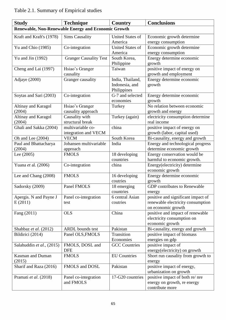
65
Table 2.1. Summary of Empirical studies
Study Technique Country Conclusions Renewable, Non-Renewable Energy and Economic Growth
Kraft and Kraft's (1978) Sims Causality United States of
America
Economic growth determine
energy consumption
Yu and Chio (1985) Co-integration United States of
America
Economic growth determine
energy consumption
Yu and Jin (1992) Granger Causality Test South Korea,
Philippine
Energy determine economic
growth
Cheng and Lai (1997) Hsiao’s Granger
causality
Taiwan positive impact of energy on
growth and employment
Adjaye (2000) Granger causality India, Thailand,
Indonesia, and
Philippines
Energy determine economic
growth
Soytas and Sari (2003) Co-integration G-7 and selected
economies
Energy determine economic
growth
Altinay and Karagol
(2004)
Hsiao’s Granger
causality approach
Turkey No relation between economic
growth and energy
Altinay and Karagol
(2004)
Causality with
structural break
Turkey (again) electricity consumption determine
real income
Ghali and Sakka (2004) multivariable co-
integration and VECM
china positive impact of energy on
growth (labor, capital used)
Oh and Lee (2004) VECM South Korea Bi-causality, energy and growth
Paul and Bhattacharya
(2004)
Johansen multivariable
approach
India Energy and technological progress
determine economic growth
Lee (2005) FMOLS 18 developing
countries
Energy conservation would be
harmful to economic growth.
Yuana et al. (2006) Co-integration china Energy(electricity) determine
economic growth
Lee and Chang (2008) FMOLS 16 developing
coutries
Energy determine economic
growth
Sadorsky (2009) Panel FMOLS 18 emerging
countries
GDP contributes to Renewable
energy
Apergis. N and Payne J
E (2011)
Panel co-integration
test
6 central Asian
coutries
positive and significant impact of
renewable electricity consumption
on economic growth
Fang (2011) OLS China positive and impact of renewable
electricity consumption on
economic growth
Shahbaz et al. (2012) ARDL bounds test Pakistan Bi-causality, energy and growth
Bildirici (2014) Panel OLS,FMOLS Transition
Economies
positive impact of biomass
energies on gdp
Salahuddin et al., (2015) FMOLS, DOSL and
DFE
GCC Countries positive impact of
energy(electricity) on growth
Kasman and Duman
(2015)
FMOLS EU Countries Short run causality from growth to
energy
Sharif and Raza (2016) FMOLS and DOSL Pakistan positive impact of energy,
urbanization on growth
Pramati et al. (2018) Panel co-integration
and FMOLS
17-G20 countries positive impact of both re/ nre
energy on growth, re energy
contribute more
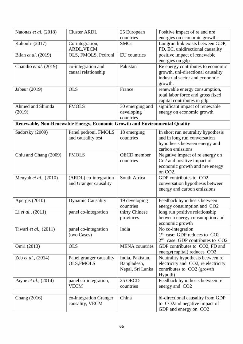
66
Natonas et al. (2018) Cluster ARDL 25 European
countries
Positive impact of re and nre
energies on economic growth.
Kahouli (2017) Co-integration,
ARDL,VECM
SMCs Longrun link exists between GDP,
FD, EC, unidirectional causality
Bilan et al. (2019) OLS, FMOLS, Pedroni EU countries positive impact of renewable
energies on gdp
Chandio et al. (2019) co-integration and
causal relationship
Pakistan Re energy contributes to economic
growth, uni-directional causality
industrial sector and economic
growth.
Jabeur (2019) OLS France renewable energy consumption,
total labor force and gross fixed
capital contributes in gdp
Ahmed and Shimda
(2019)
FMOLS 30 emerging and
developing
countries
significant impact of renewable
energy on economic growth
Renewable, Non-Renewable Energy, Economic Growth and Environmental Quality
Sadorsky (2009) Panel pedroni, FMOLS
and causality test
18 emerging
countries
In short run neutrality hypothesis
and in long run conversation
hypothesis between energy and
carbon emissions
Chiu and Chang (2009) FMOLS OECD member
countries
Negative impact of re energy on
Co2 and positive impact of
economic growth and nre energy
on CO2.
Menyah et al., (2010) (ARDL) co-integration
and Granger causality
South Africa GDP contributes to CO2
conversation hypothesis between
energy and carbon emissions
Apergis (2010) Dynamic Causality 19 developing
countries
Feedback hypothesis between
energy consumption and CO2
Li et al., (2011) panel co-integration thirty Chinese
provinces
long run positive relationship
between energy consumption and
economic growth
Tiwari et al., (2011) panel co-integration
(two Cases)
India No co-integration
1st case: GDP reduces to CO2
2nd case: GDP contributes to CO2
Omri (2013) OLS MENA countries GDP contributes to CO2, FD and
energy(capital) reduces CO2
Zeb et al., (2014) Panel granger causality
OLS,FMOLS
India, Pakistan,
Bangladesh,
Nepal, Sri Lanka
Neutrality hypothesis between re
electricity and CO2, re electricity
contributes to CO2 (growth
Hypoth)
Payne et al., (2014) panel co-integration,
VECM
25 OECD
countries
Feedback hypothesis between re
energy and CO2
Chang (2016) co-integration Granger
causality, VECM
China bi-directional causality from GDP
to CO2and negative impact of
GDP and energy on CO2
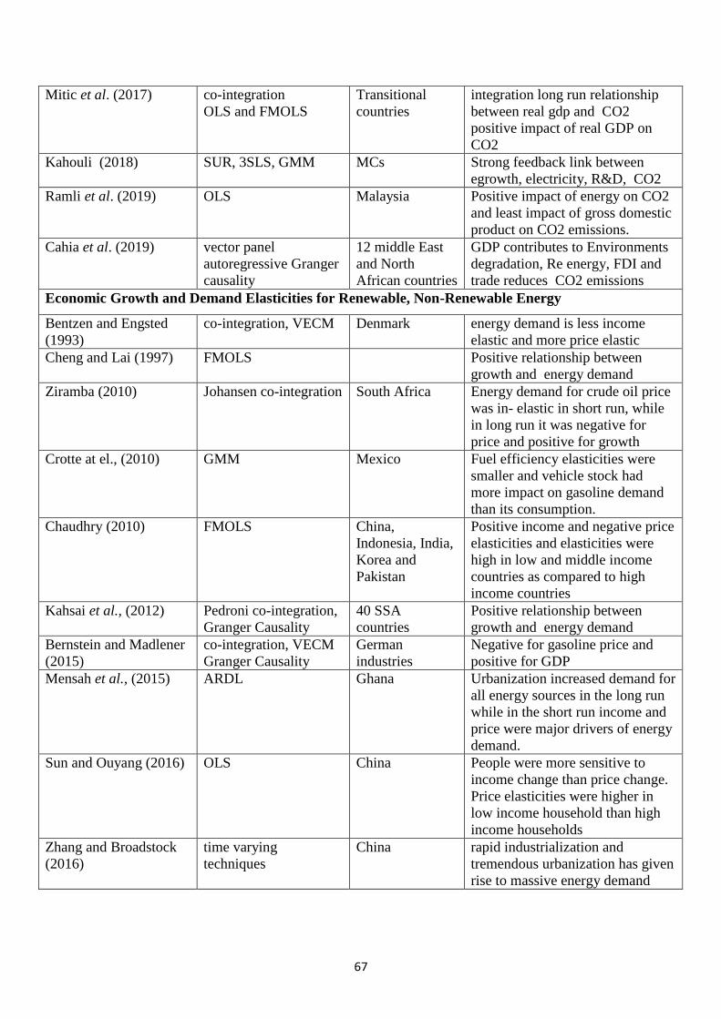
67
Mitic et al. (2017) co-integration
OLS and FMOLS
Transitional
countries
integration long run relationship
between real gdp and CO2
positive impact of real GDP on
CO2
Kahouli (2018) SUR, 3SLS, GMM MCs Strong feedback link between
egrowth, electricity, R&D, CO2
Ramli et al. (2019) OLS Malaysia Positive impact of energy on CO2
and least impact of gross domestic
product on CO2 emissions.
Cahia et al. (2019) vector panel
autoregressive Granger
causality
12 middle East
and North
African countries
GDP contributes to Environments
degradation, Re energy, FDI and
trade reduces CO2 emissions
Economic Growth and Demand Elasticities for Renewable, Non-Renewable Energy
Bentzen and Engsted
(1993)
co-integration, VECM Denmark energy demand is less income
elastic and more price elastic
Cheng and Lai (1997) FMOLS Positive relationship between
growth and energy demand
Ziramba (2010) Johansen co-integration South Africa Energy demand for crude oil price
was in- elastic in short run, while
in long run it was negative for
price and positive for growth
Crotte at el., (2010) GMM Mexico Fuel efficiency elasticities were
smaller and vehicle stock had
more impact on gasoline demand
than its consumption.
Chaudhry (2010) FMOLS China,
Indonesia, India,
Korea and
Pakistan
Positive income and negative price
elasticities and elasticities were
high in low and middle income
countries as compared to high
income countries
Kahsai et al., (2012) Pedroni co-integration,
Granger Causality
40 SSA
countries
Positive relationship between
growth and energy demand
Bernstein and Madlener
(2015)
co-integration, VECM
Granger Causality
German
industries
Negative for gasoline price and
positive for GDP
Mensah et al., (2015) ARDL Ghana Urbanization increased demand for
all energy sources in the long run
while in the short run income and
price were major drivers of energy
demand.
Sun and Ouyang (2016) OLS China People were more sensitive to
income change than price change.
Price elasticities were higher in
low income household than high
income households
Zhang and Broadstock
(2016)
time varying
techniques
China rapid industrialization and
tremendous urbanization has given
rise to massive energy demand
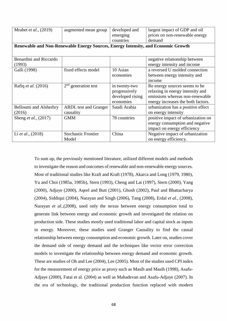
68
To sum up, the previously mentioned literature, utilized different models and methods
to investigate the reason and outcomes of renewable and non-renewable energy sources.
Most of traditional studies like Kraft and Kraft (1978), Akarca and Long (1979, 1980),
Yu and Choi (1985a, 1985b), Stern (1993), Cheng and Lai (1997), Stern (2000), Yang
(2000), Adjaye (2000), Aqeel and Butt (2001), Ghosh (2002), Paul and Bhattacharya
(2004), Siddiqui (2004), Narayan and Singh (2006), Tang (2008), Erdal et al., (2008),
Narayan et al.,(2008), used only the nexus between energy consumption total to
generate link between energy and economic growth and investigated the relation on
production side. These studies mostly used traditional labor and capital stock as inputs
in energy. Moreover, these studies used Granger Causality to find the causal
relationship between energy consumption and economic growth. Later on, studies cover
the demand side of energy demand and the techniques like vector error correction
models to investigate the relationship between energy demand and economic growth.
These are studies of Oh and Lee (2004), Lee (2005). Most of the studies used CPI index
for the measurement of energy price as proxy such as Masih and Masih (1998), Asafu-
Adjaye (2000), Fatai et al. (2004) as well as Mahadevan and Asafu-Adjaye (2007). In
the era of technology, the traditional production function replaced with modern
Mrabet et al., (2019) augmented mean group developed and
emerging
countries
largest impact of GDP and oil
prices on non-renewable energy
demand
Renewable and Non-Renewable Energy Sources, Energy Intensity, and Economic Growth
Benardini and Riccardo
(1993)
negative relationship between
energy intensity and income
Galli (1998) fixed effects model 10 Asian
economies
a reversed U molded connection
between energy intensity and
income
Rafiq et al. (2016) 2nd generation test in twenty-two
progressively
developed rising
economies
Re energy sources seems to be
relaxing in energy intensity and
emissions whereas non-renewable
energy increases the both factors.
Belloumi and Alsherhry
(2016)
ARDL test and Granger
causality
Saudi Arabia urbanization has a positive effect
on energy intensity
Sheng et al., (2017) GMM 78 countries positive impact of urbanization on
energy consumption and negative
impact on energy efficiency
Li et al., (2018) Stochastic Frontier
Model
China Negative impact of urbanization
on energy efficiency.
69
production function which used the technology as an input. In that context, the energy
used as technical input and the traditional model replacement with modified version of
STRIPAT model. Shi (2003), Fan et al. (2006), York (2007), Poumanyvong (2010),
Die and Liu (2011), Zhong and Lin (2012), Poumanyvong et al. (2012), Liddle (2014),
Shafaie and Salim (2014) and Al-Mulali, Ozturk, (2015), used the said model in various
investigations. Sadrosky (2014) also used the STRIPAT model in emerging markets.
The energy intensity and URB are used as a proxy of T (Technology). Li and Lin (2015)
used two model in STRIPAT into four groups according to their yearly income level.
The first model included the share of industry and URB in EC model as a T
(Technology). While the share of industry, URB and energy intensity are included in
the CO2 model as a T (Technology). Shahbaz et al (2015), Rafiq et al (2016) and Rauf
et al. (2018) analyzed the four model in the STRIPAT and EKC (Environmental
Kuznets curve) models.
Later studies used renewable energy and non-renewable energy instead of traditional
energy such as Apergis and Payne (2009), Amirat and Bourni (2010), Asghar and Rahat
(2011) explored the causal link between energy use and economic growth in single
country using time series data. Masih and Masih (1996), Asghar (2008), Nondo and
Kashi (2009), Noor and Saddiqi (2010), used panel data. Dogan (2015) explored the
electricity consumption from renewable and non-renewable energy sources and
economic growth. Sadorsky (2009) Apergis and Payne (2010a) extended the link
between renewable energy and income. Lee (2005), Rufael (2006), Lee and Chang
(2008), Apergis and Payne (2010b, 2011, 2011b, 2011c and 2012), Tugcu et al. (2012)
and Bhattacharya et al., (2016) Khobai and Roux (2017), Natonas et al. (2018), Jabeur
(2019) and Bilan et al. (2019) explored the causal link between renewable and non-
renewable energy use and economic growth in cross countries using panel series data.
Ahmad (2012) investigated the partial impacts of trade-openness and institutional
quality on monetary development crosswise over nations utilizing panel data collection
Emmanuel and Ebi (2013) inspected the relationship between institutional quality, oil
assets and economic development. Latter on Nayaran and Smyth (2009), Lean and
Smyth (2010), Halicioglu (2011), Shahbaz et al., (2012) included Dedeoğlu and Kaya
(2013) inquired about the association between exports, imports and energy use and
economic growth. Recently, the new studies Mitic et al. (2017), Khobai and Roux
(2017) and Bilan et al. (2019) also used the renewable energy and non-renewable
70
energy sources separately using FMOLS techniques. Bilgili et al. (2016), Al-Mulali and
Ozturk (2016), Dogan and Seker (2016b, c), and Bento and Moutinho (2016) also found
negative impact of renewable energy on CO2 emissions which mitigate the pollution
and positive impact of economic growth and non-renewable energy on CO2 emissions
which leads to pollutant environment.
In nutshell, the empirical studies recommended a number of leading indicators such as
economic growth, inflation, institution, financial development, population total,
population density, industrialization, and trade openness are found to be important in
the prospects of renewable and non-renewable energy sources. Observational based
empirical investigations likewise give rule with respect with the impact of energy on
economic development and environmental quality. Along these lines literature give a
strong base to the choice of factors to be utilized in observational investigation. At long
last, the literature proposed that there is no solid examination that talks about both the
causes and prospects of renewable and nonrenewable energy sources on account of
South Asia. The ebb and flow research study is an unassuming exertion to fill this hole.
71
CHAPTER 3
METHODOLOGY
This chapter describes and explain the research methodology in order to achieve the
targeted research objectives. The objective of this research is to explore the prospects
of renewable and non-renewable energy sources on the one hand and to analyze the
consequences of renewable and non-renewable energy sources on South Asian
Economies on the other hand. This research intends to use econometric models to
achieve research objectives. Econometrics use economic theory and statistical
influences to analyze and test economic phenomena. Economists use econometric
models to analyze the association between variables, usually with the hope of
determining causality.
3.1 Data
Four countries from the region of South Asia has been selected for empirical
investigation on the basis of data availability. These countries are India, Pakistan,
Bangladesh and Sri Lanka. The time span to be covered in the thesis is 1980-2014. See
table A1 in appendices for variable description.
3.2 Model Specification
Empirical Analysis is conducted to achieve the research objective proposed in this
study. Nine different models are utilized for empirical analysis. The first three models
explain the impact of renewable and non-renewable energy sources on economic
growth and in these models, economic growth is used as dependent variable. The next
model describes the role of renewable and non-renewable energy sources in the process
of economic development, in improving environmental quality taking per capita co2
emission as independent variable. Model 6 and 7 describe the determinants and
elasticities of renewable and non-renewable energy demand taking renewable and non-
renewable energy sources as dependent variables, respectively. The last three models
explore the relationship of energy intensity with economic growth and renewable and
non-renewable energy sources. In these models energy intensity used as dependent
variable. Summary of the all variables is given in appendices (see table B1 and B2).
72
3.2.1 Renewable and Non-Renewable Energy Sources with Economic
Growth
Kraft and Kraft (1978), Akarca and Long (1979, 1980), Yu and Choi (1985a, 1985b),
Stern (1993), Cheng and Lai (1997), Stern (2000), Yang (2000), Adjaye (2000), Aqeel
and Butt (2001), Ghosh (2002), Paul and Bhattacharya (2004), Siddiqui (2004), Oh and
Lee (2004), Lee (2005), Narayan and Singh (2006), Tang (2008), Erdal et al., (2008),
Narayan et al.,(2008), Apergis and Payne (2009), Amirat and Bourni (2010), Asghar
and Rahat (2011) explored the causal link between energy use and economic growth in
single country using time series data. Masih and Masih (1996), Asghar (2008), Nondo
and Kashi (2009), Noor and Saddiqi (2010), used panel data. Dogan (2015) explored
the electricity consumption from renewable and non-renewable energy sources and
economic growth. Sadorsky (2009) Apergis and Payne (2010a) extended the link
between renewable energy and income. Lee (2005), Rufael (2006), Lee and Chang
(2008), Apergis and Payne (2010b, 2011, 2011b, 2011c and 2012), Tugcu et al. (2012)
and Bhattacharya et al.,(2016) Khobai and Roux (2017), Natonas et al. (2018), Jabeur
(2019) and Bilan et al. (2019) explored the causal link between renewable and non-
renewable energy use and economic growth in cross countries using panel series data.
Ahmad (2012) investigated the partial impacts of trade-openness and institutional
quality on monetary development crosswise over nations utilizing panel data collection
Emmanuel and Ebi (2013) inspected the relationship between institutional quality, oil
assets and economic development. Latter on Nayaran and Smyth (2009), Lean and
Smyth (2010), Halicioglu (2011), Shahbaz et al., (2012) included Dedeoğlu and Kaya
(2013) inquired about the association between exports, imports and energy use and
economic growth.
3.2.1.1 Model 1: Relationship between Renewable and Non-renewable
Energy, Institutions and Economic Growth
The relationship between economic growth (Y), renewable energy sources (RE),
nonrenewable energy sources (NRE), institutions (INS), population density (PD) and
trade openness (To) is modeled as follows:
73
, , , ,it it it it it itY f RE NRE INS PD To 1
1 2 3 4 5it i it i it i it i it i it itY RE NRE INS PD To 2
Where
Y = GDP per capita (constant 2005 US $) is a proxy for Economic Growth
RE = Electricity production from renewable sources (kWh) is proxy for Renewable
Energy sources
NRE = Electricity production from oil sources (kWh) is proxy for Non-Renewable
Energy sources
INS = Institutions (polity 2 score obtain from polity IV is used to measure institutions)
PD = Population Density (People per square Km of land area)
To = Trade openness is measured by ratio of exports + imports to GDP
ε = Error Term
3.2.1.3 Model 2: Relationship between Renewable and Non-renewable
Energy, Urbanization and Economic Growth
The relationship between economic growth (Y), renewable energy sources (RE), non-
renewable energy sources (NRE), institutions (INS), inflation (CPI) and urbanization
(URB) is modeled as follows:
, , , ,it it it it it itY f RE NRE INS CPI URB 3
1 2 3 4 5it i it i it i it i it i it itY RE NRE INS P URB 4
Y = GDP per capita (constant 2005 US $) is a proxy for Economic Growth
RE = Electricity production from renewable sources (kWh) is proxy for Renewable
Energy sources
NRE = Electricity production from oil sources (kWh) is proxy for Non-Renewable
Energy sources
74
INS = Institutions (polity 2 score obtain from polity IV is used to measure institutions)
CPI = Consumer Price Index is used to measure inflation
URB = Urban population (% of total)
ε = Error Term
3.2.1.3. Model 3: Relationship between Renewable and Non-renewable
Energy, Financial Development and Economic Growth
Latter on Narayan and Smyth (2009), Lean and Smyth (2010), Halicioglu (2011),
Shahbaz et al., (2012) included the financial development with trade openness and
energy use from both renewable and non-renewable.
The relationship between economic growth (Y), renewable energy sources (RE),
nonrenewable energy sources (NRE), financial development (FD), population density
(PD) and trade openness (To) is modeled as follows:
, , , ,it it it it it itY f RE NRE FD PD To 5
1 2 3 4 5it i it i it i it i it i it itY RE NRE FD PD To 6
Where
Y = GDP per capita (constant 2005 US $) is a proxy for Economic Growth
RE = Electricity production from renewable sources (kWh) is proxy for Renewable
Energy sources
NRE = Electricity production from oil sources (kWh) is proxy for Non-Renewable
Energy sources
FD = Financial Development (Broad money to total reserves ratio is used to measure
FD)
PD = Population Density (People per square Km of land area)
To = Trade openness is measured by ratio of exports + imports to GDP
75
ε = Error Term
According to the empirical literature presented in the previous chapter, the coefficients
of renewable and non-renewable energy sources are expected to be positive because an
increase in energy sources may lead to increase economic growth. The coefficient of
institutions may be positive or may be negative. The coefficient of urbanization may
also be positive because urbanization process may lead to enhance economic activities.
Industrialization also have positive impact on economic growth. The coefficient of
trade openness may be positive or may be negative.
3.2.1.4. Data Sources
The data on real GDP per capita, renewable energy sources, nonrenewable energy
sources, merchandize exports, merchandise imports, inflation, and financial
development, urbanization and population density are obtained from World
Development Indicators (2014) of the World Bank. The data on polity 2 score is obtain
from polity IV project (Marshall and Jaggers, 2015). The variables real GDP per capita,
renewable energy sources, nonrenewable energy sources urbanization, financial
development, inflation, and population density are in logarithmic form.
3.2.2 Renewable and Non-Renewable Energy with Environment Quality
3.2.2.1. Model 4: Relationship between Renewable and Non-renewable
Energy, Population Density and Environment
The relationship between environmental quality (CO2), economic growth (Y),
renewable energy sources (RE), nonrenewable energy sources (NRE) and population
density (PD) is modeled as follows:
2 , , ,it it it it itCO f Y RE NRE PD 7
1 2 3 4 52it i i it i it i it i it itCO Y RE NRE PD 8
The relationship between environmental quality (CO2), economic growth (Y), square
of economic growth (Y2), renewable energy sources (RE), nonrenewable energy
sources (NRE) and population density (PD) is modeled as follows:
76
22 , , , ,it it it it it itCO f Y Y RE NRE PD 9
2
1 2 3 4 5 62it i i it i it i it i it i it itCO Y Y RE NRE PD 10
Where
CO2 = CO2 emissions (metric tons per capita)
Y = GDP per capita (constant 2005 US $) is a proxy for Economic Growth
Y2 = Square of GDP per capita (constant 2005 US $) is a proxy for Economic Growth.
RE = Electricity production from renewable sources (kWh) is proxy for Renewable
Energy sources
NRE = Electricity production from oil sources (kWh) is proxy for Non-Renewable
Energy sources
PD = Population Density (People per square Km of land area)
ε = Error Term
3.2.2.2. Model 5: Relationship between Renewable and Non-renewable
Energy, Urbanization, Energy Intensity and Environment
The relationship between environmental quality (CO2), economic growth (Y),
renewable energy sources (RE), nonrenewable energy sources (NRE), urban population
(%) of total, economic efficiency and population density (PD) is modeled as follows:
2 , , , , ,it it it it it it itCO f Y RE NRE PT URB EI 11
1 2 3 4 6 7 82it i i it i it i it i it i it i it itCO Y RE NRE PT URB EI 12
Environmental Kuznets hypothesis is presented as:
22 , , , , , ,it it it it it it it itCO f Y Y RE NRE PT URB EI 13
Its general form can be written as:
77
2
1 2 3 4 5 6 7 82it i i it i it i it it i it i it i it itCO Y Y RE NRE PT URB EI 14
Where
CO2 = CO2 emissions (metric tons per capita)
Y = GDP per capita (constant 2005 US $) is a proxy for Economic Growth.
Y2 = Square of GDP per capita (constant 2005 US $) is a proxy for Economic Growth.
RE = Electricity production from renewable sources (kWh) is proxy for Renewable
Energy sources
NRE = Electricity production from oil sources (kWh) is proxy for Non-Renewable
Energy sources
URB = Urban population (% of total)
EI = EI = Energy Intensity measured by ratio of total energy consumption to GDP
PT = Population Total
ε = Error Term
According to the empirical literature presented in the previous chapter, the coefficient
of renewable energy sources are expected to be negative because an increase in energy
sources may lead to decrease in per capita CO2 emissions so, renewable energy sources
are environment friendly. The coefficient of non-renewable energy sources are
expected to be positive because an increase in energy sources may lead to increase in
per capita CO2 emissions. The coefficient of urbanization may also be positive because
urbanization process may lead to enhance per capita CO2 emissions. Industrialization
also have positive impact on per capita CO2 emissions. The coefficient of trade
openness may be positive or may be negative. Population total or population density
may also increase pollution so the coefficients of population total and population
density are expected to be positive. The coefficient of energy intensity also expected to
be positive.
78
The mentioned above model is the modified version of STRIPAT model. The
specification of the STRIPAT model is:
I =aPibAi
cTidui 15
In the above equation, a is the constant term, while b, c and d are the responsiveness of
environmental impact on P, A, and T correspondingly. The variables µ denotes the error
term and the subscript i represent the country analysis. Shi (2003), Fan et al. (2006),
York (2007), Poumanyvong (2010), Die and Liu (2011), Zhong and Lin(2012),
Poumanyvong et al. (2012), Liddle (2014), Shafaie and Salim (2014) and Al-Mulali,
Ozturk, (2015), Mitic et al. (2017), Khobai and Roux (2017) and Bilan et al. (2019)
used the said model in various investigations. Sadrosky (2014) also used the STRIPAT
model in emerging markets. The energy intensity and URB are used as a proxy of T
(Technology). Li and Lin (2015) used two model in STRIPAT into four groups
according to their yearly income level. The first model included the share of industry
and URB in EC model as a T (Technology). While the share of industry, URB and
energy intensity are included in the CO2 model as a T (Technology). Shahbaz et al
(2015), Rafiq et al (2016) and Rauf et al. (2018) analyzed the four model in the
STRIPAT and EKC (Environmental Kuznets curve) models.
3.2.2.3. Data Sources
The data on per capita CO2 emissions, real GDP per capita, renewable energy sources,
nonrenewable energy sources, merchandize exports, merchandize imports and
population density are obtained from World Development Indicators (latest version) of
the World Bank. The data on polity 2 score is obtain from polity IV project (Marshall
and Jaggers, 2015). The variables per capita CO2 emissions, real GDP per capita,
renewable energy sources, nonrenewable energy sources and population density are in
logarithmic form.
3.2.3. Demand Elasticity of Renewable and Non-Renewable Energy
Sources
3.2.3.1. Model 6: Relationship between Renewable Energy Demand,
Economic Growth, Industrialization, Technological Changes and Energy
Price
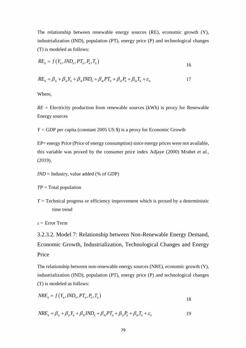
79
The relationship between renewable energy sources (RE), economic growth (Y),
industrialization (IND), population (PT), energy price (P) and technological changes
(T) is modeled as follows:
, , , ,it it it it it itRE f Y IND PT P T 16
1 2 3 4 5 6it i i it i it i it i it i it itRE Y IND PT P T 17
Where,
RE = Electricity production from renewable sources (kWh) is proxy for Renewable
Energy sources
Y = GDP per capita (constant 2005 US $) is a proxy for Economic Growth
EP= energy Price (Price of energy consumption) since energy prices were not available,
this variable was proxed by the consumer price index Adjaye (2000) Mrabet et al.,
(2019).
IND = Industry, value added (% of GDP)
TP = Total population
T = Technical progress or efficiency improvement which is proxed by a deterministic
time trend
ε = Error Term
3.2.3.2. Model 7: Relationship between Non-Renewable Energy Demand,
Economic Growth, Industrialization, Technological Changes and Energy
Price
The relationship between non-renewable energy sources (NRE), economic growth (Y),
industrialization (IND), population (PT), energy price (P) and technological changes
(T) is modeled as follows:
, , , ,it it it it it itNRE f Y IND PT P T 18
1 2 3 4 5 6it i i it i it i it i it i it itNRE Y IND PT P T 19
80
Where,
Y= real GDP per capita (constant 2005 US $ used as proxy of economic growth)
NRE = Non-renewable energy sources proxied by electricity production from oil
sources (kWh)
P= energy Price (Price of energy consumption) since energy prices were not available,
this variable was proxied by the consumer price index (Akinlo, 2008; Galindo, 2005;
Hondroyiannis et al., 2002; Adjaye, 2000; Mrabet et al., (2019).
IND = Industry, value added (% of GDP)
TP = Total population
T = Technical progress or efficiency improvement which is proxies by a deterministic
time trend
ε = Error Term
According to the studies of Rapanos and Polemis (2006), Hunt and Ninomiya (2005)
and Fouquet et al. (1997), the coefficient of economic growth is expected to be positive
because an increase in economic growth may lead to increase in demand for both
renewable and non-renewable energy sources. The coefficient of industrialization
(value share of industry) is also expected to be positive because an increase in value
share of industry in terms of GDP designates the industrialization process and may lead
to increase in demand for both renewable and non-renewable energy sources
Samoulidis and Mitropoulos (1984). The coefficient of population is expected to be
positive because an increase in population may lead to increase in demand for both
renewable and non-renewable energy sources. The coefficient of energy price is
expected to be negative, an increase in energy price leads to reduction in energy demand
according to Pindyck (1979a) higher energy prices have contributed to lower economic
growth and may lead to change in lifestyles of many nations which leads to reduce
energy demand. Another important determinant of demand for energy is technical
efficiency. In this thesis, the improvement in energy efficiency has been captured by
the standard approach of a deterministic time trend. According to the studies of
Beenstock and Willcock (1981), Kouris (1983), Hunt et al. (2003) and Dimitropolus et
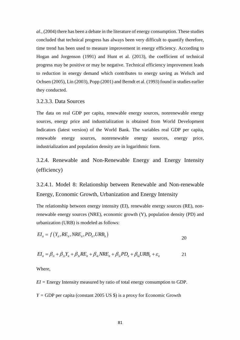
81
al., (2004) there has been a debate in the literature of energy consumption. These studies
concluded that technical progress has always been very difficult to quantify therefore,
time trend has been used to measure improvement in energy efficiency. According to
Hogan and Jorgenson (1991) and Hunt et al. (2013), the coefficient of technical
progress may be positive or may be negative. Technical efficiency improvement leads
to reduction in energy demand which contributes to energy saving as Welsch and
Ochsen (2005), Lin (2003), Popp (2001) and Berndt et al. (1993) found in studies earlier
they conducted.
3.2.3.3. Data Sources
The data on real GDP per capita, renewable energy sources, nonrenewable energy
sources, energy price and industrialization is obtained from World Development
Indicators (latest version) of the World Bank. The variables real GDP per capita,
renewable energy sources, nonrenewable energy sources, energy price,
industrialization and population density are in logarithmic form.
3.2.4. Renewable and Non-Renewable Energy and Energy Intensity
(efficiency)
3.2.4.1. Model 8: Relationship between Renewable and Non-renewable
Energy, Economic Growth, Urbanization and Energy Intensity
The relationship between energy intensity (EI), renewable energy sources (RE), non-
renewable energy sources (NRE), economic growth (Y), population density (PD) and
urbanization (URB) is modeled as follows:
, , , ,it it it it it itEI f Y RE NRE PD URB 20
1 2 3 4 5 6it i i it i it i it i it i it itEI Y RE NRE PD URB 21
Where,
EI = Energy Intensity measured by ratio of total energy consumption to GDP.
Y = GDP per capita (constant 2005 US $) is a proxy for Economic Growth
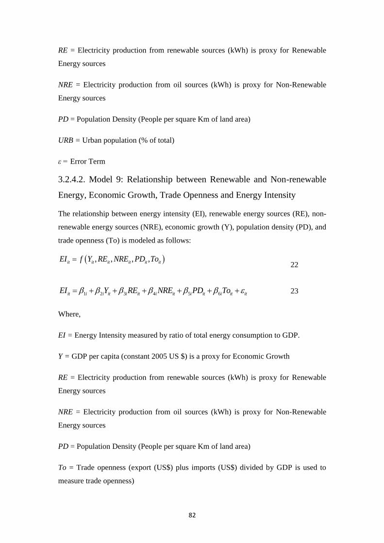
82
RE = Electricity production from renewable sources (kWh) is proxy for Renewable
Energy sources
NRE = Electricity production from oil sources (kWh) is proxy for Non-Renewable
Energy sources
PD = Population Density (People per square Km of land area)
URB = Urban population (% of total)
ε = Error Term
3.2.4.2. Model 9: Relationship between Renewable and Non-renewable
Energy, Economic Growth, Trade Openness and Energy Intensity
The relationship between energy intensity (EI), renewable energy sources (RE), non-
renewable energy sources (NRE), economic growth (Y), population density (PD), and
trade openness (To) is modeled as follows:
, , , ,it it it it it itEI f Y RE NRE PD To 22
1 2 3 4 5 6it i i it i it i it i it i it itEI Y RE NRE PD To 23
Where,
EI = Energy Intensity measured by ratio of total energy consumption to GDP.
Y = GDP per capita (constant 2005 US $) is a proxy for Economic Growth
RE = Electricity production from renewable sources (kWh) is proxy for Renewable
Energy sources
NRE = Electricity production from oil sources (kWh) is proxy for Non-Renewable
Energy sources
PD = Population Density (People per square Km of land area)
To = Trade openness (export (US$) plus imports (US$) divided by GDP is used to
measure trade openness)
83
ε = Error Term
3.2.4.3. Model 10: Relationship between Renewable and Non-renewable
Energy, Economic Growth, Industrialization, Technological Progress and
Energy Intensity
The relationship between energy intensity (EI), renewable energy sources (RE), non-
renewable energy sources (NRE), economic growth (Y), population density (PD),
industrialization (IND) and technological changes (T) is modeled as follows:
, , , , ,it it it it it it itEI f Y RE NRE PD IND T 24
1 2 3 4 5 6 7it i i it i it i it i it i it i it itEI Y RE NRE PD IND T 25
Where,
EI = Energy Intensity measured by ratio of total energy consumption to GDP.
Y = GDP per capita (constant 2005 US $) is a proxy for Economic Growth
RE = Electricity production from renewable sources (kWh) is proxy for Renewable
Energy sources
NRE = Electricity production from oil sources (kWh) is proxy for Non-Renewable
Energy sources
PD = Population Density (People per square Km of land area)
IND = Industry, value added (% of GDP)
T = Technical progress or efficiency improvement which is peroxide by a deterministic
time trend
ε = Error Term
3.2.4.4. Data Sources
The data on total energy consumption, gross domestic product, real GDP per capita,
renewable energy sources, nonrenewable energy sources, merchandize exports,
merchandise imports, urbanization and population density are obtained from World
84
Development Indicators (latest version) of the World Bank. The variables energy
intensity, real GDP per capita, renewable energy sources, nonrenewable energy sources
urbanization and population density are in logarithmic form.
3.3. Econometrics Methodology
3.3.1. Time-Series Methodology
Time-series methods on unit roots, co-integration and causality are commonly applied
in individual country analysis. The brief detail of proposed time-series methodology is
provided below.
3.3.1.1. Unit Root Tests
In time series analysis, it is necessary that data should be stationary. The most
commonly used test of unit root in time series data is the augmented Dickey-Fuller
(ADF) test in which the null hypothesis is non-stationary. ADF test is sensitive to lag
length selection and the presence of negative MA term. This test is also characterized
by problem of poor power and size. In contrast to this test, DF-GLS unit root test
proposed by Elliott, Rothenberg and Stock (1996) have higher power in the sense
that this test is more likely to reject the null hypothesis of a unit root and accept
the alternative hypothesis of stationary. This test is also called de-trending test because
it is used to determine the order of integration of the variables Zt. Further, this test
requires much shorter sample sizes than the conventional ADF tests to attain the same
statistical power. The general equation of DF-GLS test is given below:
* * *
1 1 1 1 1....d d d d
t t t p t p tz z z z 26
Where d
tz the de-trended series and null hypothesis of this test is that tz has a random
walk trend:
0 1ˆ ˆd
t tz z t 27
The DF-GLS test proposed two hypothesis. Firstly tz is stationary with a linear time
trend and secondly, it is stationary without linear time trend with a mean greater than
zero. The test is performed by utilizing the generalized least square technique in an
85
alternative hypothesis. This estimation is investigated by generating the following
variables:
2, 1 ,....., 1t Tz z L z L z
28
2, 1 ,....., 1t TY z L Y L Y
29
And 1, 1tY tT
30
Where T represents the number of observations for tz and is fixed. OLS estimation
is followed by the under given equation:
0 1 t tz Y Y 31
OLS estimators 0 and 1 are utilized for the removal of trend from tz above. OLS is
employed on the transformed variable by fitting the following regression:
0 1
1
md d d
t t i t i t
i
z z z
32
Finally, ADF regression is employed on new transformed variables and test the null
hypothesis: 0 : 0H
3.3.1.2. Johansen Co-integration Test
The concept of co-integration was first introduced by Granger (1981) and elaborated
further by Engle and Granger (1987), Engle and Granger (1987) give the formal
definition of co-integration among two as follows: “ time series Yt and Xt are said to
be co-integration of order d, b where d ≥ b ≥ 0, written as Yt, Xt ̃ CI(d, b) if (a) both
series are integrated of order d, (b) there exist a linear combination of these variables,
say
β1Yt + β 2 Xt which is integrated of order d-b. The vector {β1 β2} is called the co-
integration vector.”
This analysis is used to capture the notion that non-stationary variables may possess
long run equilibrium relationship so that they tend to move together in the long run.
86
The concept of the co-integration is characterized by a situation where the variables in
a given relation should not diverge from each other in the long run. (Banerjee et. al.,
1993)
The presence of a unit root (non-stationary time series) in time series may lead to
spurious development of theory. The individual time series may be I(1), that is they
have stochastic trend, their linear combination may be stationary and the series are said
to be co-integrated. (Gujarati, 2006)
The stationary linear combination is called the co-integration equation. We first identify
the co-integrating relationship i.e., determination of the rank of the matrix Π. When the
rank is zero, it implies that Π. contains only zero elements, on the other hand, an “n”
rank shows that all endogenous variables in the model are I(0). Johansen suggested two
test to determine the rank ‘r’ or the number of co-integration equation.
1. The Trace Test
2. The Maximum Eigen value Test
4.3.4.1. The Trace Test
The Trace test is based upon a sequence of hypothesis tests. The test statistics will be:
LR trace (γ Ho ) = - T ∑ ln (1- λi) 34
Where (γ Ho ) is the number of co-integration equations assuming the null hypothesis is
true and λˆi is the estimated Eigenvalue.
The test sequence is as follows:
r = 0 versus r ≥ 1
Ho : r = 0 (There are no co-integrating equations)
H1 : r ≥ 1 (There are r ≥ 1 co-integration equation)
r = 1 versus r ≥ 2
Ho : r = 1 (There are r = 1 co-integrating equations)
H1 : r ≥ 2 (There are r ≥ 2 co-integration equation)
87
And the sequence continues, until we have hypotheses test:
r = n-1 versus r = n
Ho : r = n-1 (There are (n-1) co-integrating equations)
H1 : r = n (There are maximum co-integration equation)
If LR trace (γ Ho ) > critical values reject Ho in favour of H1 otherwise accept Ho.
If the test indicates the presence of co-integrating combination in the model, error
correction can be applied to it that gives us information about long run equilibrium
relationship and short run dynamics.
4.2.4.2. The Maximum Eigenvalue Test
The test statistics will be:
LR max (γ Ho ) = - n ln (1- λ r Ho +1) 35
This test is also based on the sequence of the hypothesis test thus; the testing sequence
is as follows:
r = 0 versus r = 1
Ho : r = 0 (There are no co-integrating equations)
H1 : r = 1 (There are r = 1 co-integration equation)
The second hypothesis test is
r = 1 versus r = 2
Ho : r = 1 (There are r = 1 co-integrating equations)
H1 : r = 2 (There are r = 2 co-integration equation)
And the sequence continues, until we have the (n-1) th hypothesis test:
r = n-1 versus r = n
Ho : r = n-1 (There are (n-1) co-integrating equations)
H1 : r = n (There are maximum co-integration equation)
88
The thesis have been applied the standard maximum likelihood technique of Johansen
and Juselius (1990) and Johanson (1995) to determine the long run relationship
between the variables or to check whether the variables are co-integrated or not.
3.3.2 Panel Data Methodology
Panel data have two important merits with respect to time series data. Firstly, such data
is large in sample size, more efficient and more reliable and have less co linearity among
variables. Secondly, panel data enables researchers to include country specific affects
and time specific effects to absorb the effects of unobservable variables that are
correlated with explanatory variables included in the panel (Reppas and Chirstopoulos,
2005).
In short, panel data analysis provides large sample size and hence more powerful
significance tests as compared to time-series analysis. This is true not only for unit root
tests but also for co-integration tests. In this section, detail of panel co-integration tests
and panel data causality analysis are provided.
3.3.2.1. Panel Unit Root Tests
The study apply Levine et al. 2002 (LLC), Im et al. 2003 (IPS) with demean panel unit
root tests to check the stationary properties of the variables. These tests apply to a
balanced panel but the LLC can be considered a pooled panel unit root test, IPS
represents as a heterogeneous panel test. Some recent papers (Lyhagen, 2008 and
Wagner, 2008) find that in the presence of cross-sectional dependence (particularly in
the case of trade openness and economic growth due to unobservable common shocks),
the IPS, LLC and other similar tests incorrectly reject the null hypothesis of non-
stationary. Therefore, we also implement the unit root tests on time demeaned series to
deal with cross-sectional dependence. According to Levin et al. (2002), implementing
unit root tests on time demeaned series allows to mitigate the impact of cross-sectional
dependence on panel data.
3.3.2.2 LLC Unit Root Test
Levin et al. (2002) developed a number of pooled panel unit root tests with various
specifications depending upon the treatment of the individual specific intercepts and
time trends. This test imposes homogeneity on the autoregressive coefficient that
89
indicates the presence or absence of unit root problem while the intercept and the trend
can vary across individual series. LLC unit root test follows ADF regression for the
investigation of unit root hypothesis is given below step by step:
1. Implement a separate ADF regression for each country:
ti
p
j
jtijiitiiti
i
yyy ,
1
,,1,
36
The lag order pi is allowable to across individual countries. The appropriate lag length
is chosen by allowing the maximum lag order and then uses the t-statistics for ij b to
determine if a smaller lag order is preferred.
2. Run two separate regressions and save the residuals 1,
~~
, tiit
itti
p
j
jtijtiiti
i
yy~
,
1
,,,
37
1,
~
1,
1
,,1,
titi
p
j
jtijtiiti
i
yy 38
LLC procedure suggests standardized the errors 1,
~~
, tiit by the regressing the standard
error the ADF equation provided above:
^
1,
~
1
~
^
~
~
,
i
ti
it
i
it
it
39
3. Regression can be run to compute the panel test statistics following equation-v:
titiit ,1,
~~
40
The null hypothesis is as follows: 0......,..: 1 nH and alternate hypothesis
is 0......: nAH .
90
3.3.2.2 IPS Unit Root Test
Im, Pesaran and Shin (IPS), (2003) introduced a panel unit root test in the context of a
heterogeneous panel. This test basically applies the ADF test to individual series thus
allowing each series to have its own short-run dynamics. But the overall t-test statistic
is based on the arithmetic mean of all individual countries’ ADF statistic. Suppose a
series ( tiTR , tiEC ) can be represented by the ADF (without trend).
ti
p
j
jtijitiijti
i
xxx ,
1
,,1,,
41
After the ADF regression has different augmentation lags for each country in finite
samples, the term )( TtE and )var( Tt are replaced by the corresponding group averages
of the tabulated values of ),( iT PtE and T ivar (t ,P ) respectively. The IPS test allows for
the heterogeneity in the value i under the alternative hypothesis. This is more efficient
and powerful test than usual single time series test. The estimable equation of IPS unit
root test is modeled as following:
)(1
, i
N
i
tiNT PtN
It
42
wheretit ,is the ADF t-statistics for the unit root tests of each country and iP is the lag
order in the ADF regression and test statistic can be calculated as following:
T T
tT
N(T)[t E(t )]
var(t )
43
As NTt is explained above and values for )]0,([ iiT PtE can be obtained from the results
of Monte Carlo simulation carried out by IPS. They have calculated and tabulated them
for various time periods and lags. When the ADF has different augmentation lags )( iP
91
the two terms )( TtE and )var( Tt in the equation above are replaced by corresponding
group averages of the tabulated values of ),( iT PtE and ),var( iT Pt respectively2.
3.3.3 The Panel Co-integration Tests
Advance panel co-integration tests can be expected to have high power than the
traditional tests. The tests applied for long-run examination are developed by Larsson
et al., (2001).
The panel Larsson et al., (2001) likelihood ratio test statistics is derived from the
average of the individual likelihood ratio test statistics of Johanson (1995). The
multivariate co-integration trace test of Johanson (1988, 1995) is engaged to investigate
each individual cross-section system autonomously, in such a way, allowing
heterogeneity in each cross-sectional unit root for said panel. The process of data
generation for each of the groups is characterized by following heterogeneous VAR (
ip ) model:
tijti
p
j
jiti YYi
,,
1
,,
44
Where TtNi ,.......1;,......,1
For each one, the value of 0,1, ,...... iji YY is considered fixed and
ti, are independent and
identically distributed (normally distributed): ),0(~ iKN , where i is the cross-
2Karlsson and Lothgren, (2000) demonstrate the power of panel unit root tests by Monte Carlo
simulation. The null of all these tests is that each series contains a unit root and thus is difference
stationary. However, the alternative hypothesis is not clearly specified. In LLC the alternative is that all
individual series in the panel are stationary. In IPS the alternative is that at least one of the individual
series in the panel is stationary. They conclude that the “presence or absence of power against the
alternative where a subset of the series is stationary has a serious implications for empirical work. If
the tests have high power, a rejection of the unit root null can be driven by few stationary series and
the whole panel may inaccurately be modelled as stationary. If, on other hand, the tests have low power
it may incorrectly concluded that the panel contains a common unit root even if a majority of the series
is stationary’’ (p. 254). The simulation results reveal that the power of the tests (LLC, IPS) increases
monotonically with: (1) an increased number (N) of the series in the panel; (2) an increased time series
dimension (T) in each individual series; (3) increased proportion of stationary series in the panel. Their
Monte Carlo simulations for N=13 and T=80 reveal the power of the test is 0.7 for LLC tests and
approaching unity for the IPS tests.
92
correlation matrix in the error terms: ),( '
,, titii E . The equation-10 can be
modified in vector error correction model (VECM) model as given below:
jijti
p
j
jitiiti YYYi
,,
1
1
,1,,
45
Where 1......1, piiiand
ijijiji ,1,,,is of order )( kk . If i is
of reduced rank: rank ii r )( , which can be decomposed into 'abi , where i and
i are of order )( irk and of full rank column rank that represents the error correction
form. The null hypotheses of panel LLL (2001) rank test are:
0 i iH rank ( ) r r for all Ni ,.....,1 against
a iH rank ( ) k for all Ni ,.....,1
The procedure is in sequences like individual trace test process for cointegration rank
determination. First, we test for 0 i iH rank( ) r r, r 0 , if null hypothesis of no
co-integration is accepted, this shows that there is no co-integration relationship
i i(rank ( ) r 0) in all cross-sectional groups for said panel. If null hypothesis is not
accepted then null hypothesis 1r is tested. The sequence of procedure is not
disconnected and continued until null hypothesis is accepted, 1 kr , is rejected.
Accepting the hypothesis of co-integration 0r along with null hypothesis of rank
i( ) r 0 (0 r k) implies that there is at least one cross-sectional unit in panel
which has rank 0)( ri . The likelihood ratio trace test statistic for group i is as
following;
)1ln()(/)((ln2)(/)({1
'
p
rl
liiTiT TkHrHQkHrHLR 46
Where '
l is the thl largest eigen value in the thi cross-section unit. The LR-bar statistic
is calculated as the average of individual trace statistics:
)](/)([1
)](/)([1
_
kHrHLRN
kHrHRLn
i
iTiT
47
93
Finally, modified version of above equation is defined as:
_
_
NT k
LRk
N(LR [H(r) / H(k)]) E(Z )[H(r) / H(k)]
VAR(Z )
48
Where )( kZE and )( kZVar are mean and variance of the asymptotic trace statistics,
which can be obtained from simulation. The LLL (2001) prove the central limit theorem
for the standard LR-bar statistic that under the null hypothesis, _
LR
N(0,1) as N and
T in such a way that 1
NT 0,
under the assumption that there is no cross-
correlation in the error terms, that is give below:
i,tE( ) 0 and i
i,t j,tE( , )0
for jiji , 49
LLL (2001) note that T is needed for each of the individual test statistic to
converge to its asymptotic distribution, while N is needed for the central limit
theorem.
3.3.3.1 Estimation of Panel Co-integration Regression
On the off chance that all the variables are co-integrated, the following stride is to assess
the long-run co-integration parameters. Within the incidence of co-integration, an
Ordinary Least Square estimator is recognized as biased and conflicting results. Due to
behind this cause, limited estimators have been offered. For instance, Kao and Chiang
(2000) contend that their parametric panel Dynamic OLS (DOLS) estimator (that pools
the information along the inside measurement of the board) is promising in small
samples and performs well when all is said in done in co-integrated panels. Be that as
it may, the panel DOLS because of Kao and Chiang (2000) does not consider the
significance of cross-sectional heterogeneity in the alternative hypothesis. To take into
consideration cross-sectional heterogeneity in the alternative hypothesis, endogeneity
and serial correlation problems to get steady and asymptotically unbiased estimates of
the co-integrating vectors, Pedroni (2000; 2001) proposed the group mean Fully
Modified OLS (FMOLS) estimator for co-integrated panels. These methodologies used
by the authors in their papers such as Sadorsky, P. (2009), Apergis & Payne (2010a),
Fang, Y. (2011), Al-Mulali et al., (2013) Sadorsky.P (2014), Cho et al., (2016), Jebli
94
et al., (2016), Mitic et al. (2017), Jabeur (2019) Ahmed and Shimda (2019) Ramli et
al., (2019, Natonas et al., (2018) and Bilan et al. ,(2019).
Taking after Pedroni (2001), FMOLS method produces predictable estimates in small
samples and does not suffer from large size distortions in the presence of endogeneity
and heterogeneous progression. The board FMOLS estimator for the coefficient β is
characterized as:
1
1 2 *
1 1 1
ˆ ˆ( ) ( )
N T T
it it it i
i t t
N y y y y z T 50
Where * 0 021 21
21 21 22 22
22 22
ˆ ˆˆ ˆˆ ˆˆ( ) , ( )
ˆ ˆi i
it it it i i i i i
i i
L Lz z z y
L L and ˆ
iL is a
lower triangular decomposition of ˆi . The associated t-statistics gives:
* *
1/2
ˆ ˆ ,1
N
ii
t N t
Where *
1/2
* 1 2
ˆ 0 11,1
ˆ ˆ ( )
T
i i itit
t y y 51
3.4.3.2 Panel Granger Causality Test
The panel Co-integration tests imply the presence of the long runs affiliation among
variables, but it does not notify regarding the direction of the affiliation amongst the
variables. If the relationships of variables are existed, the Granger causality test can be
utilized to research the causal connection amongst the variables. We used the more
advanced form of causality test Granger (1969) for panel data, which is developed by
Hurlin and Venet (2001). Mathematical equation which is utilized is explained below:
( ) ( )
, , ,
1 0
p pk k
it i t k i t k i t
k k
Y y z w
52
Where assume the coefficient of autoregressive( )k and the slopes of equation ( )k
i
remain constant. The null and alternative hypothesis is defined below:
H0: 0i 11,....,i N
H1: 0i 1 11, 2,....,i N N N
95
Where N1 is unknown but satisfies the condition 0< N1/N<1. The formation of this test
is similar to unit root test in a heterogeneous panel presented by IPS (2003). We process
the following Wald Statistics with a specific goal to test these Np linear restrictions:
2 1
1
( ) / ( )
RSS / (1 )hnc
RSS RSS NpF
NT N p p
53
Where RSS2 is the restricted residual sum of square while RSS1 is the unrestricted
residual sum of squares of above equation. HNC hypothesis is accepted if the calculated
value of F-statistics is not significant.
The panel Granger Causality test is also measured in the light of W & Z test
measurements of the Homogenous Non Causality (HNC) theory. In the test, the null
hypothesis of Homogenous Non Causality (HNC) hypothesis implies there is no
relationship for all the cross-units of the panel. Under the alternative, there is a
relationship among variables in the long run. This test is applied on a balance data. The
W measurements compare to the cross sectional normal of the N standard individual
Wald statistics of Granger non-causality tests. The Z measurements compare to the
standardized statistic (for fixed T sample). Both measurements tend to a normal
distribution when both T and N dimension tends to infinity (forW ) or only when N
tends to infinity (for Z ).
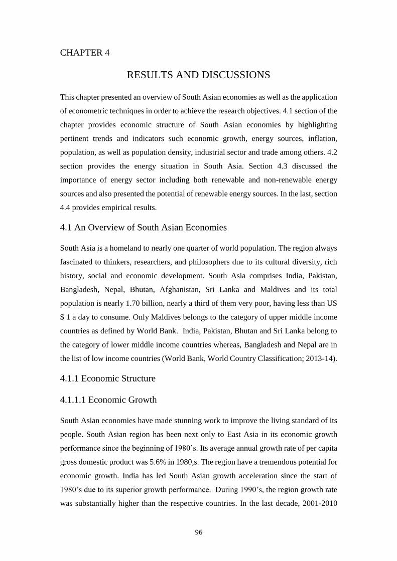
96
CHAPTER 4
RESULTS AND DISCUSSIONS
This chapter presented an overview of South Asian economies as well as the application
of econometric techniques in order to achieve the research objectives. 4.1 section of the
chapter provides economic structure of South Asian economies by highlighting
pertinent trends and indicators such economic growth, energy sources, inflation,
population, as well as population density, industrial sector and trade among others. 4.2
section provides the energy situation in South Asia. Section 4.3 discussed the
importance of energy sector including both renewable and non-renewable energy
sources and also presented the potential of renewable energy sources. In the last, section
4.4 provides empirical results.
4.1 An Overview of South Asian Economies
South Asia is a homeland to nearly one quarter of world population. The region always
fascinated to thinkers, researchers, and philosophers due to its cultural diversity, rich
history, social and economic development. South Asia comprises India, Pakistan,
Bangladesh, Nepal, Bhutan, Afghanistan, Sri Lanka and Maldives and its total
population is nearly 1.70 billion, nearly a third of them very poor, having less than US
$ 1 a day to consume. Only Maldives belongs to the category of upper middle income
countries as defined by World Bank. India, Pakistan, Bhutan and Sri Lanka belong to
the category of lower middle income countries whereas, Bangladesh and Nepal are in
the list of low income countries (World Bank, World Country Classification; 2013-14).
4.1.1 Economic Structure
4.1.1.1 Economic Growth
South Asian economies have made stunning work to improve the living standard of its
people. South Asian region has been next only to East Asia in its economic growth
performance since the beginning of 1980’s. Its average annual growth rate of per capita
gross domestic product was 5.6% in 1980,s. The region have a tremendous potential for
economic growth. India has led South Asian growth acceleration since the start of
1980’s due to its superior growth performance. During 1990’s, the region growth rate
was substantially higher than the respective countries. In the last decade, 2001-2010
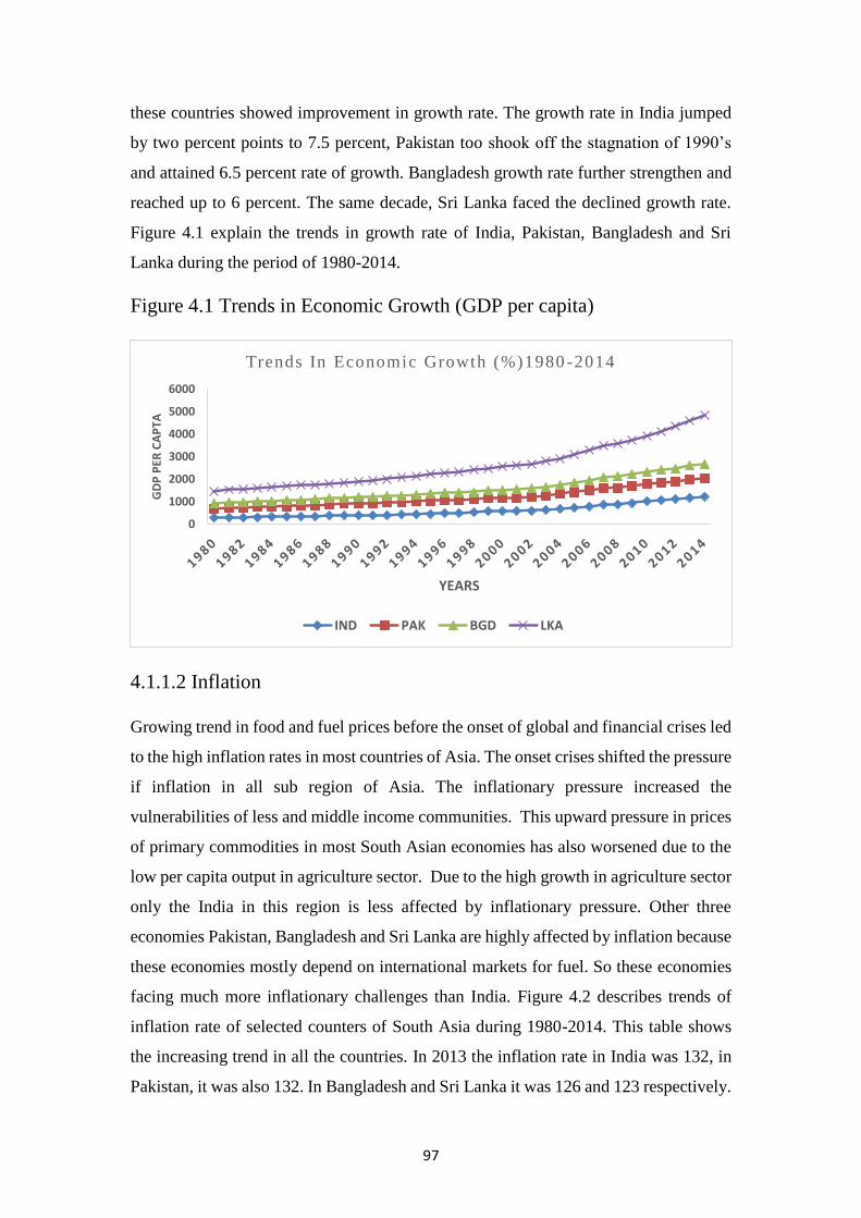
97
these countries showed improvement in growth rate. The growth rate in India jumped
by two percent points to 7.5 percent, Pakistan too shook off the stagnation of 1990’s
and attained 6.5 percent rate of growth. Bangladesh growth rate further strengthen and
reached up to 6 percent. The same decade, Sri Lanka faced the declined growth rate.
Figure 4.1 explain the trends in growth rate of India, Pakistan, Bangladesh and Sri
Lanka during the period of 1980-2014.
Figure 4.1 Trends in Economic Growth (GDP per capita)
4.1.1.2 Inflation
Growing trend in food and fuel prices before the onset of global and financial crises led
to the high inflation rates in most countries of Asia. The onset crises shifted the pressure
if inflation in all sub region of Asia. The inflationary pressure increased the
vulnerabilities of less and middle income communities. This upward pressure in prices
of primary commodities in most South Asian economies has also worsened due to the
low per capita output in agriculture sector. Due to the high growth in agriculture sector
only the India in this region is less affected by inflationary pressure. Other three
economies Pakistan, Bangladesh and Sri Lanka are highly affected by inflation because
these economies mostly depend on international markets for fuel. So these economies
facing much more inflationary challenges than India. Figure 4.2 describes trends of
inflation rate of selected counters of South Asia during 1980-2014. This table shows
the increasing trend in all the countries. In 2013 the inflation rate in India was 132, in
Pakistan, it was also 132. In Bangladesh and Sri Lanka it was 126 and 123 respectively.
0
1000
2000
3000
4000
5000
6000
GD
P P
ER C
AP
TA
YEARS
Trends In Economic Growth (%)1980 -2014
IND PAK BGD LKA
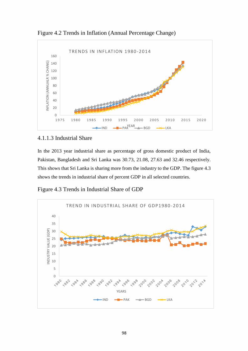
98
Figure 4.2 Trends in Inflation (Annual Percentage Change)
4.1.1.3 Industrial Share
In the 2013 year industrial share as percentage of gross domestic product of India,
Pakistan, Bangladesh and Sri Lanka was 30.73, 21.08, 27.63 and 32.46 respectively.
This shows that Sri Lanka is sharing more from the industry to the GDP. The figure 4.3
shows the trends in industrial share of percent GDP in all selected countries.
Figure 4.3 Trends in Industrial Share of GDP
0
20
40
60
80
100
120
140
160
1 9 7 5 1 9 8 0 1 9 8 5 1 9 9 0 1 9 9 5 2 0 0 0 2 0 0 5 2 0 1 0 2 0 1 5 2 0 2 0
INFL
ATI
ON
(A
NN
UA
LR %
CH
AN
G)
YEAR
TRENDS IN INFLATION 1980 -2014
IND PAK BGD LKA
0
5
10
15
20
25
30
35
40
IND
UST
RY
VA
LUE
(GD
P)
YEARS
TREND IN INDUSTRIAL SHARE OF GDP1980 -2014
IND PAK BGD LKA
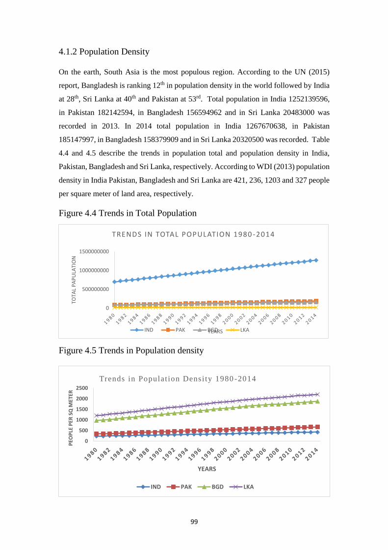
99
4.1.2 Population Density
On the earth, South Asia is the most populous region. According to the UN (2015)
report, Bangladesh is ranking 12th in population density in the world followed by India
at 28th, Sri Lanka at 40th and Pakistan at 53rd. Total population in India 1252139596,
in Pakistan 182142594, in Bangladesh 156594962 and in Sri Lanka 20483000 was
recorded in 2013. In 2014 total population in India 1267670638, in Pakistan
185147997, in Bangladesh 158379909 and in Sri Lanka 20320500 was recorded. Table
4.4 and 4.5 describe the trends in population total and population density in India,
Pakistan, Bangladesh and Sri Lanka, respectively. According to WDI (2013) population
density in India Pakistan, Bangladesh and Sri Lanka are 421, 236, 1203 and 327 people
per square meter of land area, respectively.
Figure 4.4 Trends in Total Population
Figure 4.5 Trends in Population density
0
500000000
1000000000
1500000000
TOTA
L P
AP
ULA
TIO
N
YEARS
TRENDS IN TOTAL POPULATION 1980 -2014
IND PAK BGD LKA
0
500
1000
1500
2000
2500
PEO
PLE
PER
SQ
MET
ER
YEARS
Trends in Populat ion Densi ty 1980 -2014
IND PAK BGD LKA
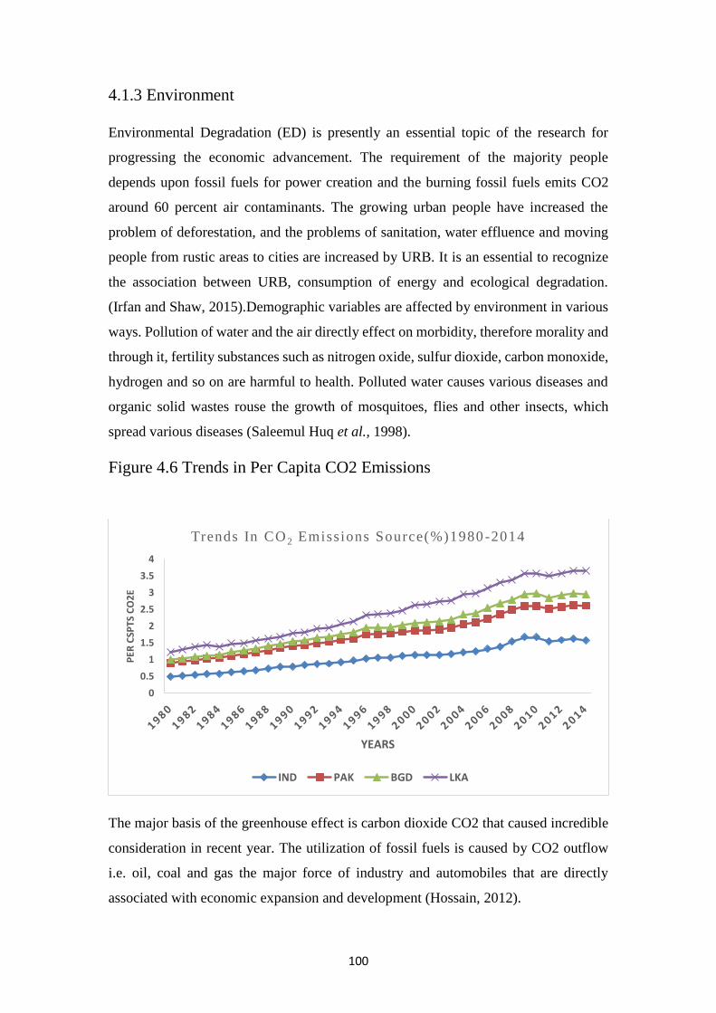
100
4.1.3 Environment
Environmental Degradation (ED) is presently an essential topic of the research for
progressing the economic advancement. The requirement of the majority people
depends upon fossil fuels for power creation and the burning fossil fuels emits CO2
around 60 percent air contaminants. The growing urban people have increased the
problem of deforestation, and the problems of sanitation, water effluence and moving
people from rustic areas to cities are increased by URB. It is an essential to recognize
the association between URB, consumption of energy and ecological degradation.
(Irfan and Shaw, 2015).Demographic variables are affected by environment in various
ways. Pollution of water and the air directly effect on morbidity, therefore morality and
through it, fertility substances such as nitrogen oxide, sulfur dioxide, carbon monoxide,
hydrogen and so on are harmful to health. Polluted water causes various diseases and
organic solid wastes rouse the growth of mosquitoes, flies and other insects, which
spread various diseases (Saleemul Huq et al., 1998).
Figure 4.6 Trends in Per Capita CO2 Emissions
The major basis of the greenhouse effect is carbon dioxide CO2 that caused incredible
consideration in recent year. The utilization of fossil fuels is caused by CO2 outflow
i.e. oil, coal and gas the major force of industry and automobiles that are directly
associated with economic expansion and development (Hossain, 2012).
0
0.5
1
1.5
2
2.5
3
3.5
4
PER
CSP
TS C
O2
E
YEARS
Trends In CO 2 Emissions Source(%)1980-2014
IND PAK BGD LKA
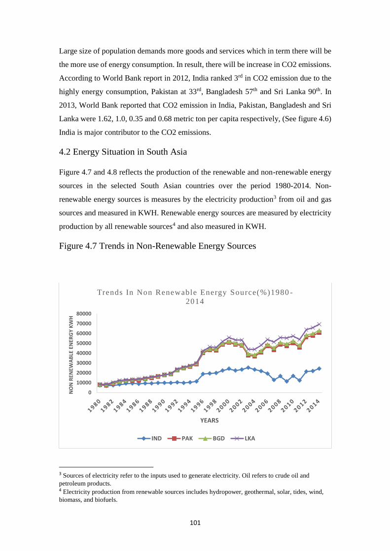
101
Large size of population demands more goods and services which in term there will be
the more use of energy consumption. In result, there will be increase in CO2 emissions.
According to World Bank report in 2012, India ranked 3rd in CO2 emission due to the
highly energy consumption, Pakistan at 33rd, Bangladesh 57th and Sri Lanka 90th. In
2013, World Bank reported that CO2 emission in India, Pakistan, Bangladesh and Sri
Lanka were 1.62, 1.0, 0.35 and 0.68 metric ton per capita respectively, (See figure 4.6)
India is major contributor to the CO2 emissions.
4.2 Energy Situation in South Asia
Figure 4.7 and 4.8 reflects the production of the renewable and non-renewable energy
sources in the selected South Asian countries over the period 1980-2014. Non-
renewable energy sources is measures by the electricity production3 from oil and gas
sources and measured in KWH. Renewable energy sources are measured by electricity
production by all renewable sources4 and also measured in KWH.
Figure 4.7 Trends in Non-Renewable Energy Sources
3 Sources of electricity refer to the inputs used to generate electricity. Oil refers to crude oil and
petroleum products. 4 Electricity production from renewable sources includes hydropower, geothermal, solar, tides, wind,
biomass, and biofuels.
0
10000
20000
30000
40000
50000
60000
70000
80000
NO
N R
ENEW
AB
LE E
NER
GY
KW
H
YEARS
Trends In Non Renewable Energy Source(%)1980 -
2014
IND PAK BGD LKA
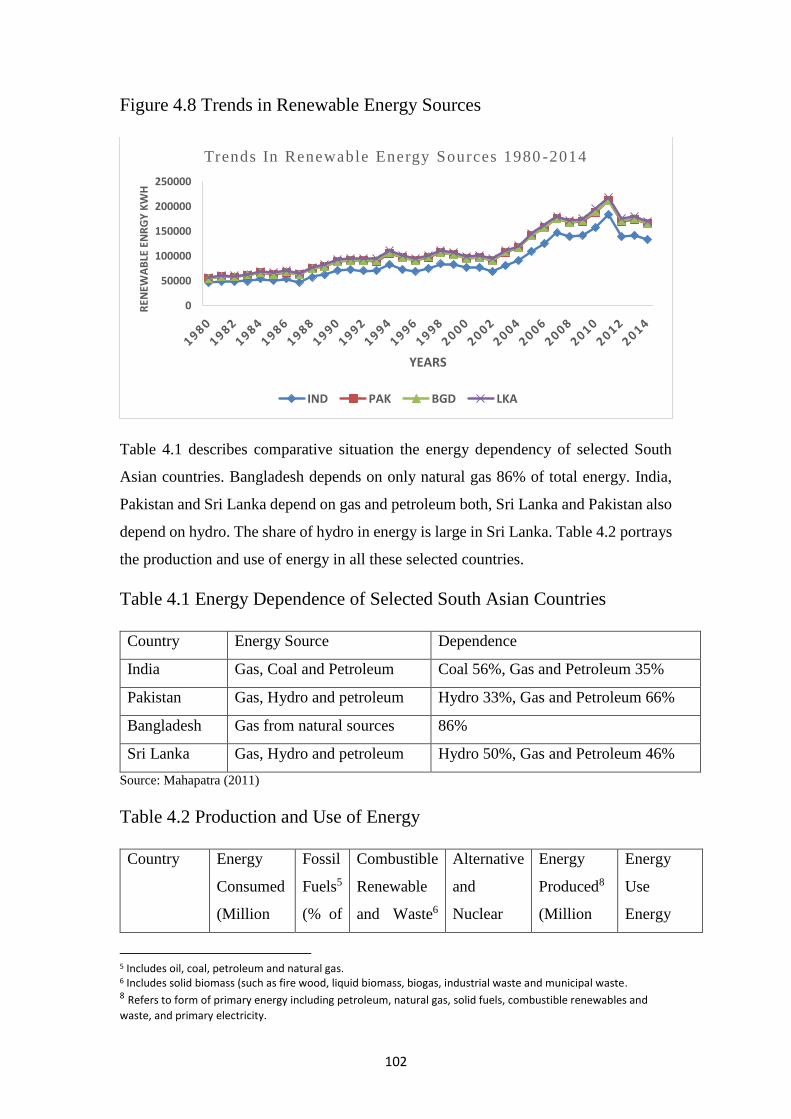
102
Figure 4.8 Trends in Renewable Energy Sources
Table 4.1 describes comparative situation the energy dependency of selected South
Asian countries. Bangladesh depends on only natural gas 86% of total energy. India,
Pakistan and Sri Lanka depend on gas and petroleum both, Sri Lanka and Pakistan also
depend on hydro. The share of hydro in energy is large in Sri Lanka. Table 4.2 portrays
the production and use of energy in all these selected countries.
Table 4.1 Energy Dependence of Selected South Asian Countries
Country Energy Source Dependence
India Gas, Coal and Petroleum Coal 56%, Gas and Petroleum 35%
Pakistan Gas, Hydro and petroleum Hydro 33%, Gas and Petroleum 66%
Bangladesh Gas from natural sources 86%
Sri Lanka Gas, Hydro and petroleum Hydro 50%, Gas and Petroleum 46%
Source: Mahapatra (2011)
Table 4.2 Production and Use of Energy
Country Energy
Consumed
(Million
Fossil
Fuels5
(% of
Combustible
Renewable
and Waste6
Alternative
and
Nuclear
Energy
Produced8
(Million
Energy
Use
Energy
5 Includes oil, coal, petroleum and natural gas. 6 Includes solid biomass (such as fire wood, liquid biomass, biogas, industrial waste and municipal waste. 8 Refers to form of primary energy including petroleum, natural gas, solid fuels, combustible renewables and
waste, and primary electricity.
0
50000
100000
150000
200000
250000
REN
EWA
BLE
EN
RG
Y K
WH
YEARS
Trends In Renewable Energy Sources 1980 -2014
IND PAK BGD LKA
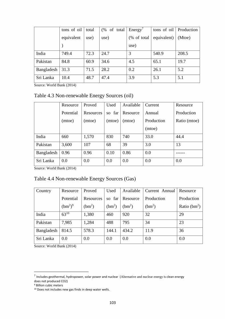
103
tons of oil
equivalent
)
total
use)
(% of total
use)
Energy7
(% of total
use)
tons of oil
equivalent)
Production
(Mtoe)
India 749.4 72.3 24.7 3 540.9 208.5
Pakistan 84.8 60.9 34.6 4.5 65.1 19.7
Bangladesh 31.3 71.5 28.2 0.2 26.1 5.2
Sri Lanka 10.4 48.7 47.4 3.9 5.3 5.1
Source: World Bank (2014)
Table 4.3 Non-renewable Energy Sources (oil)
Resource
Potential
(mtoe)
Proved
Resources
(mtoe)
Used
so far
(mtoe)
Available
Resource
(mtoe)
Current
Annual
Production
(mtoe)
Resource
Production
Ratio (mtoe)
India 660 1,570 830 740 33.0 44.4
Pakistan 3,600 107 68 39 3.0 13
Bangladesh 0.96 0.96 0.10 0.86 0.0 ------
Sri Lanka 0.0 0.0 0.0 0.0 0.0 0.0
Source: World Bank (2014)
Table 4.4 Non-renewable Energy Sources (Gas)
Country Resource
Potential
(bm2)9
Proved
Resources
(bm2)
Used
so far
(bm2)
Available
Resource
(bm2)
Current Annual
Production
(bm2)
Resource
Production
Ratio (bm2)
India 6310 1,380 460 920 32 29
Pakistan 7,985 1,284 488 795 34 23
Bangladesh 814.5 578.3 144.1 434.2 11.9 36
Sri Lanka 0.0 0.0 0.0 0.0 0.0 0.0
Source: World Bank (2014)
7 Includes geothermal, hydropower, solar power and nuclear (Alternative and nuclear energy is clean energy
does not produced CO2) 9 Billion cubic meters 10 Does not includes new gas finds in deep water wells.
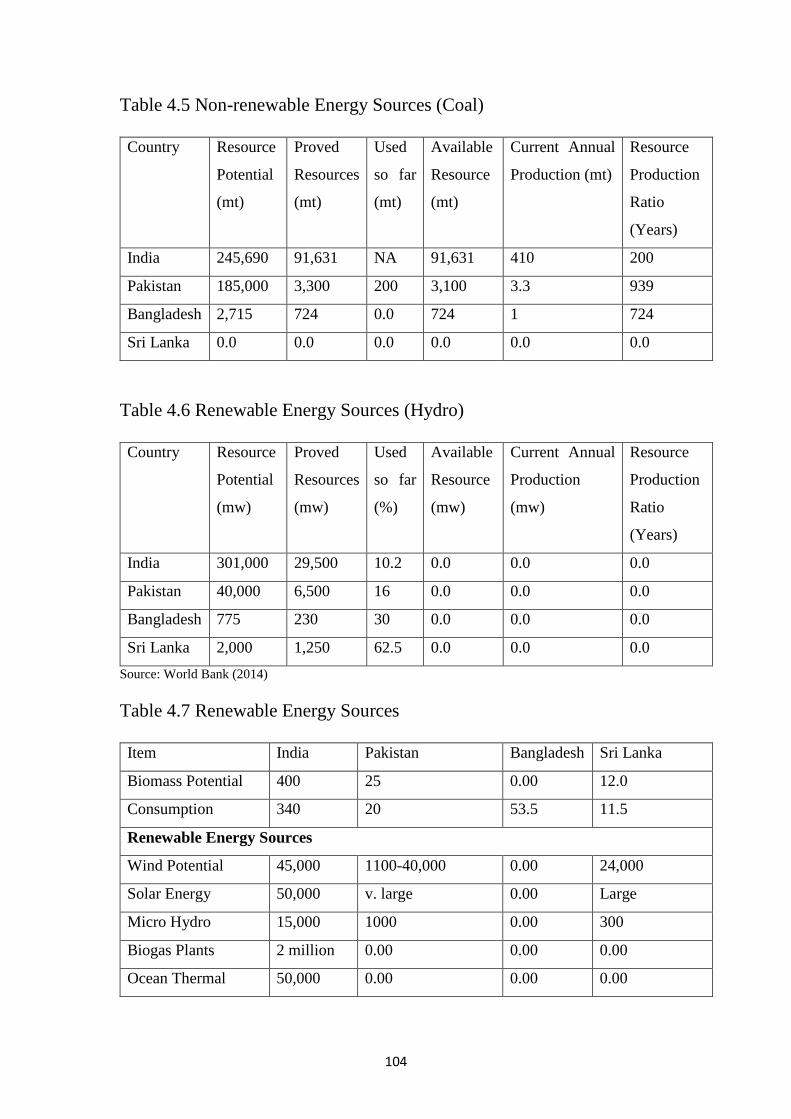
104
Table 4.5 Non-renewable Energy Sources (Coal)
Country Resource
Potential
(mt)
Proved
Resources
(mt)
Used
so far
(mt)
Available
Resource
(mt)
Current Annual
Production (mt)
Resource
Production
Ratio
(Years)
India 245,690 91,631 NA 91,631 410 200
Pakistan 185,000 3,300 200 3,100 3.3 939
Bangladesh 2,715 724 0.0 724 1 724
Sri Lanka 0.0 0.0 0.0 0.0 0.0 0.0
Table 4.6 Renewable Energy Sources (Hydro)
Country Resource
Potential
(mw)
Proved
Resources
(mw)
Used
so far
(%)
Available
Resource
(mw)
Current Annual
Production
(mw)
Resource
Production
Ratio
(Years)
India 301,000 29,500 10.2 0.0 0.0 0.0
Pakistan 40,000 6,500 16 0.0 0.0 0.0
Bangladesh 775 230 30 0.0 0.0 0.0
Sri Lanka 2,000 1,250 62.5 0.0 0.0 0.0
Source: World Bank (2014)
Table 4.7 Renewable Energy Sources
Item India Pakistan Bangladesh Sri Lanka
Biomass Potential 400 25 0.00 12.0
Consumption 340 20 53.5 11.5
Renewable Energy Sources
Wind Potential 45,000 1100-40,000 0.00 24,000
Solar Energy 50,000 v. large 0.00 Large
Micro Hydro 15,000 1000 0.00 300
Biogas Plants 2 million 0.00 0.00 0.00
Ocean Thermal 50,000 0.00 0.00 0.00
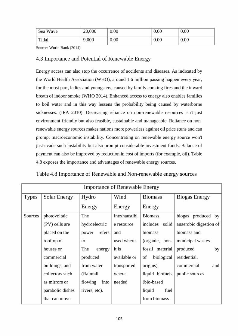
105
Sea Wave 20,000 0.00 0.00 0.00
Tidal 9,000 0.00 0.00 0.00
Source: World Bank (2014)
4.3 Importance and Potential of Renewable Energy
Energy access can also stop the occurrence of accidents and diseases. As indicated by
the World Health Association (WHO), around 1.6 million passing happen every year,
for the most part, ladies and youngsters, caused by family cooking fires and the inward
breath of indoor smoke (WHO 2014). Enhanced access to energy also enables families
to boil water and in this way lessens the probability being caused by waterborne
sicknesses. (IEA 2010). Decreasing reliance on non-renewable resources isn't just
environment-friendly but also feasible, sustainable and manageable. Reliance on non-
renewable energy sources makes nations more powerless against oil price stuns and can
prompt macroeconomic instability. Concentrating on renewable energy source won't
just evade such instability but also prompt considerable investment funds. Balance of
payment can also be improved by reduction in cost of imports (for example, oil). Table
4.8 exposes the importance and advantages of renewable energy sources.
Table 4.8 Importance of Renewable and Non-renewable energy sources
Importance of Renewable Energy
Types Solar Energy Hydro
Energy
Wind
Energy
Biomass
Energy
Biogas Energy
Sources photovoltaic
(PV) cells are
placed on the
rooftop of
houses or
commercial
buildings, and
collectors such
as mirrors or
parabolic dishes
that can move
The
hydroelectric
power refers
to
The energy
produced
from water
(Rainfall
flowing into
rivers, etc).
Inexhaustibl
e resource
and
used where
it is
available or
transported
where
needed
Biomass
includes solid
biomass
(organic, non-
fossil material
of biological
origins),
liquid biofuels
(bio-based
liquid fuel
from biomass
biogas produced by
anaerobic digestion of
biomass and
municipal wastes
produced by
residential,
commercial and
public sources
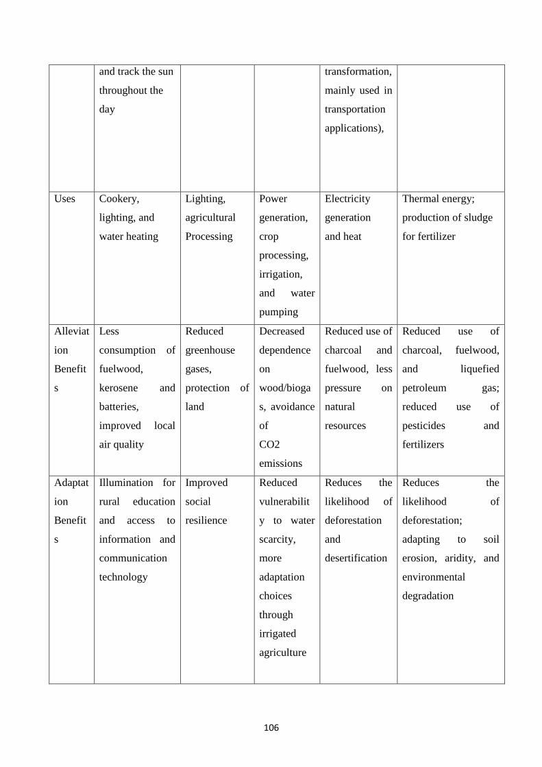
106
and track the sun
throughout the
day
transformation,
mainly used in
transportation
applications),
Uses Cookery,
lighting, and
water heating
Lighting,
agricultural
Processing
Power
generation,
crop
processing,
irrigation,
and water
pumping
Electricity
generation
and heat
Thermal energy;
production of sludge
for fertilizer
Alleviat
ion
Benefit
s
Less
consumption of
fuelwood,
kerosene and
batteries,
improved local
air quality
Reduced
greenhouse
gases,
protection of
land
Decreased
dependence
on
wood/bioga
s, avoidance
of
CO2
emissions
Reduced use of
charcoal and
fuelwood, less
pressure on
natural
resources
Reduced use of
charcoal, fuelwood,
and liquefied
petroleum gas;
reduced use of
pesticides and
fertilizers
Adaptat
ion
Benefit
s
Illumination for
rural education
and access to
information and
communication
technology
Improved
social
resilience
Reduced
vulnerabilit
y to water
scarcity,
more
adaptation
choices
through
irrigated
agriculture
Reduces the
likelihood of
deforestation
and
desertification
Reduces the
likelihood of
deforestation;
adapting to soil
erosion, aridity, and
environmental
degradation
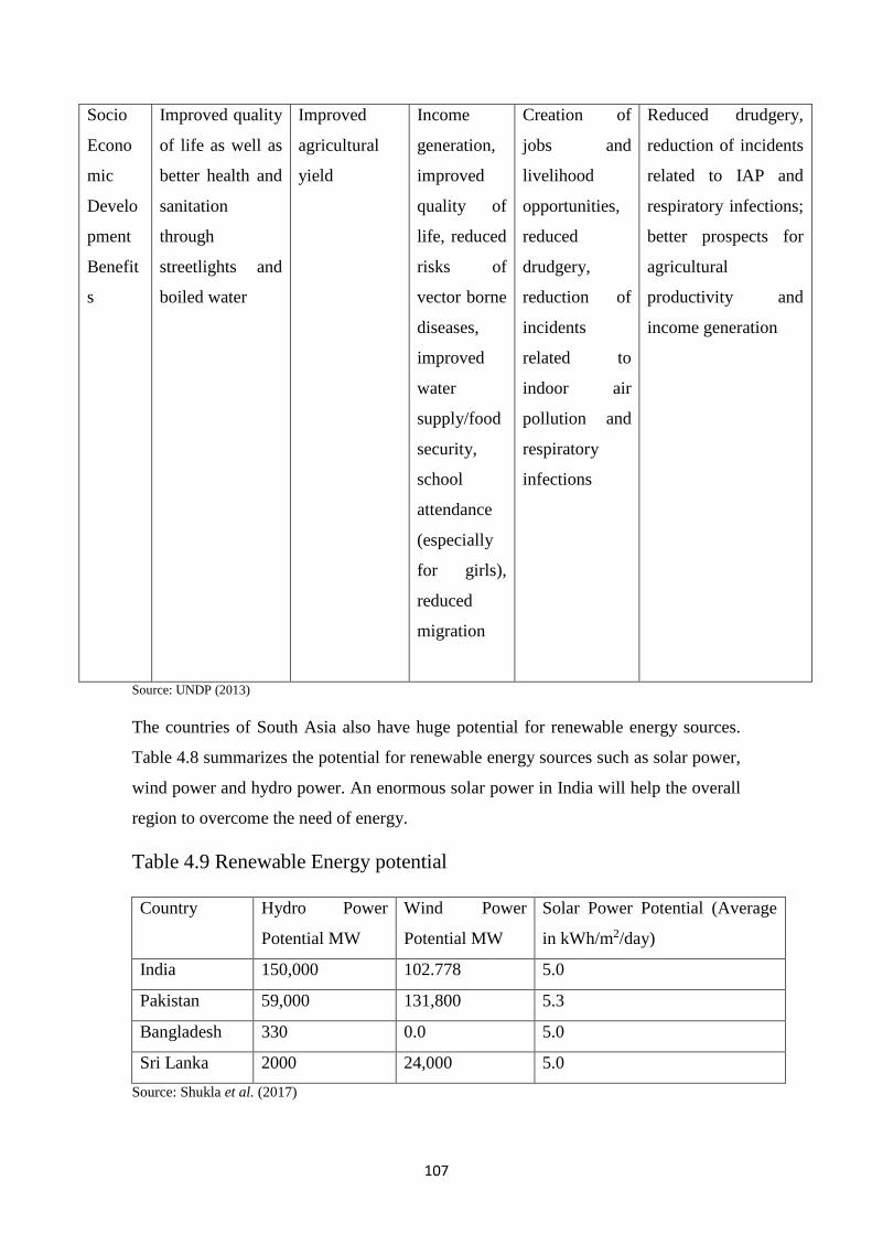
107
Socio
Econo
mic
Develo
pment
Benefit
s
Improved quality
of life as well as
better health and
sanitation
through
streetlights and
boiled water
Improved
agricultural
yield
Income
generation,
improved
quality of
life, reduced
risks of
vector borne
diseases,
improved
water
supply/food
security,
school
attendance
(especially
for girls),
reduced
migration
Creation of
jobs and
livelihood
opportunities,
reduced
drudgery,
reduction of
incidents
related to
indoor air
pollution and
respiratory
infections
Reduced drudgery,
reduction of incidents
related to IAP and
respiratory infections;
better prospects for
agricultural
productivity and
income generation
Source: UNDP (2013)
The countries of South Asia also have huge potential for renewable energy sources.
Table 4.8 summarizes the potential for renewable energy sources such as solar power,
wind power and hydro power. An enormous solar power in India will help the overall
region to overcome the need of energy.
Table 4.9 Renewable Energy potential
Country Hydro Power
Potential MW
Wind Power
Potential MW
Solar Power Potential (Average
in kWh/m2/day)
India 150,000 102.778 5.0
Pakistan 59,000 131,800 5.3
Bangladesh 330 0.0 5.0
Sri Lanka 2000 24,000 5.0
Source: Shukla et al. (2017)
108
4.4 Empirical Results and Discussions
4.4.1 Impact of Renewable and Non-Renewable Energy on
Economic Growth
4.4.1.1 Model 1: Relationship between Renewable and Non-renewable
Energy, Institutions and Economic Growth
4.4.1.1.1 Time Series Results
4.4.1.1.1.1 Unit Root Test Results
There is a basic need to check the stationary properties of the series under consideration
before assessing the log-run relationships among variables. There are numerous
contentions with respect to the use of customary unit root tests. It is obvious from
econometric that ADF tests have low power against the null hypothesis and therefore it
is important to apply other tests like KPSS and DF-GLS to confirm the results of ADF
tests. For present analysis, DF-GLS test is applied both at level and first differences
with constant and with both constant and trend. For the analysis, the null hypothesis of
unit root may be rejected if the calculated values of DF-GLS tests is greater than their
critical values. These critical values are used in absolute terms. In other words the null
hypothesis of unit root is accepted when the calculated values of DF-GLS tests is less
than their critical values (in absolute terms). Similarly, a series is said to be stationary
when the calculated values of DF-GLS tests is greater than their respective critical
values (in absolute terms).
Table 4.10 reports the unit root outcomes of DF GLS test within the sight of trend and
intercept both and only with intercept. The outcomes propose the non-stationery of all
the series at their level shape, however stationary at first difference. According to this
table, the considered variables in selected sample like economic growth (Y), renewable
energy sources (RE), nonrenewable energy sources (NRE), institutions (INS),
population density (PD) and trade openness (To) are integrated at I(1) for individual
country.
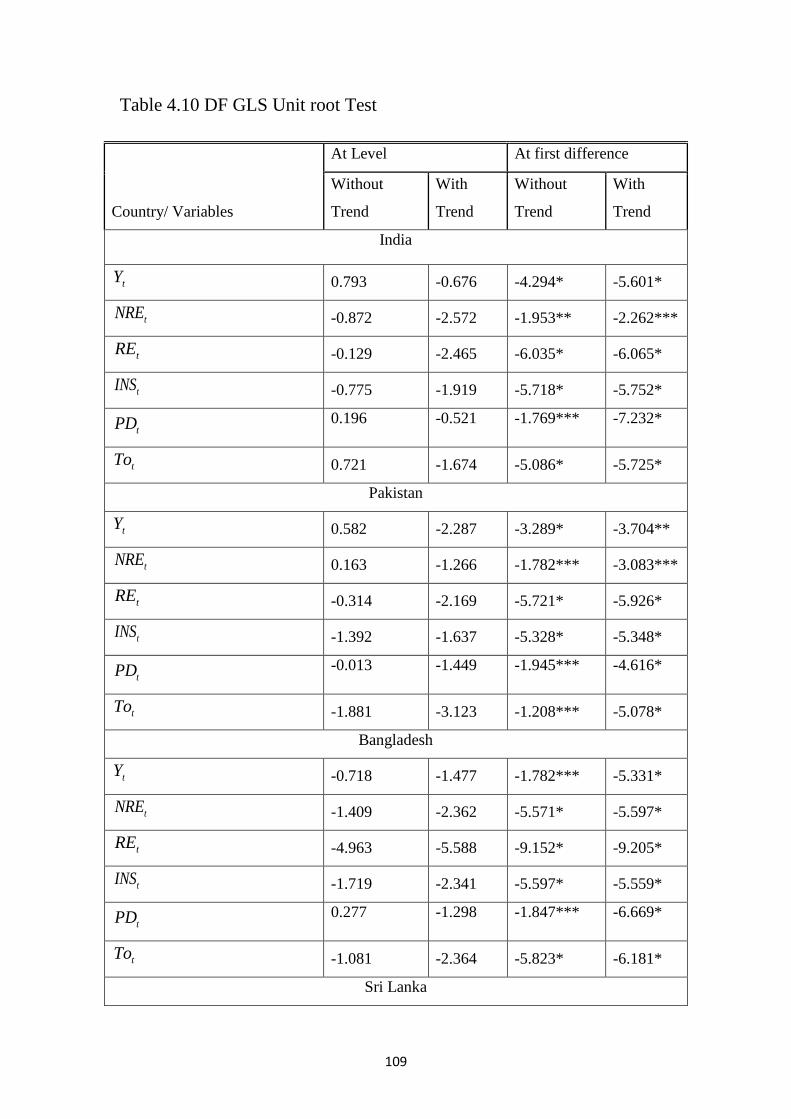
109
Table 4.10 DF GLS Unit root Test
Country/ Variables
At Level At first difference
Without
Trend
With
Trend
Without
Trend
With
Trend
India
tY 0.793 -0.676 -4.294* -5.601*
tNRE -0.872 -2.572 -1.953** -2.262***
tRE -0.129 -2.465 -6.035* -6.065*
tINS -0.775 -1.919 -5.718* -5.752*
tPD 0.196 -0.521 -1.769*** -7.232*
tTo 0.721 -1.674 -5.086* -5.725*
Pakistan
tY 0.582 -2.287 -3.289* -3.704**
tNRE 0.163 -1.266 -1.782*** -3.083***
tRE -0.314 -2.169 -5.721* -5.926*
tINS -1.392 -1.637 -5.328* -5.348*
tPD -0.013 -1.449 -1.945*** -4.616*
tTo -1.881 -3.123 -1.208*** -5.078*
Bangladesh
tY -0.718 -1.477 -1.782*** -5.331*
tNRE -1.409 -2.362 -5.571* -5.597*
tRE -4.963 -5.588 -9.152* -9.205*
tINS -1.719 -2.341 -5.597* -5.559*
tPD 0.277 -1.298 -1.847*** -6.669*
tTo -1.081 -2.364 -5.823* -6.181*
Sri Lanka
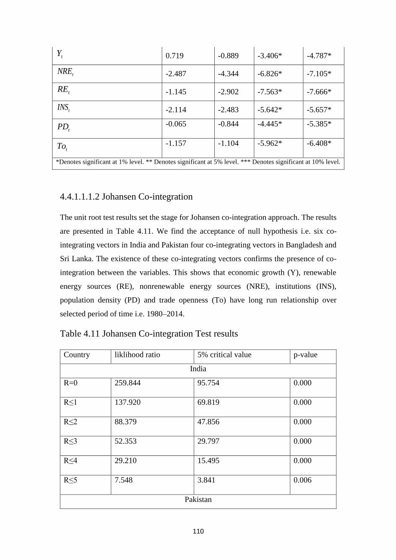
110
4.4.1.1.1.2 Johansen Co-integration
The unit root test results set the stage for Johansen co-integration approach. The results
are presented in Table 4.11. We find the acceptance of null hypothesis i.e. six co-
integrating vectors in India and Pakistan four co-integrating vectors in Bangladesh and
Sri Lanka. The existence of these co-integrating vectors confirms the presence of co-
integration between the variables. This shows that economic growth (Y), renewable
energy sources (RE), nonrenewable energy sources (NRE), institutions (INS),
population density (PD) and trade openness (To) have long run relationship over
selected period of time i.e. 1980–2014.
Table 4.11 Johansen Co-integration Test results
Country liklihood ratio 5% critical value p-value
India
R=0 259.844 95.754 0.000
R≤1 137.920 69.819 0.000
R≤2 88.379 47.856 0.000
R≤3 52.353 29.797 0.000
R≤4 29.210 15.495 0.000
R≤5 7.548 3.841 0.006
Pakistan
tY 0.719 -0.889 -3.406* -4.787*
tNRE -2.487 -4.344 -6.826* -7.105*
tRE -1.145 -2.902 -7.563* -7.666*
tINS -2.114 -2.483 -5.642* -5.657*
tPD -0.065 -0.844 -4.445* -5.385*
tTo -1.157 -1.104 -5.962* -6.408*
*Denotes significant at 1% level. ** Denotes significant at 5% level. *** Denotes significant at 10% level.
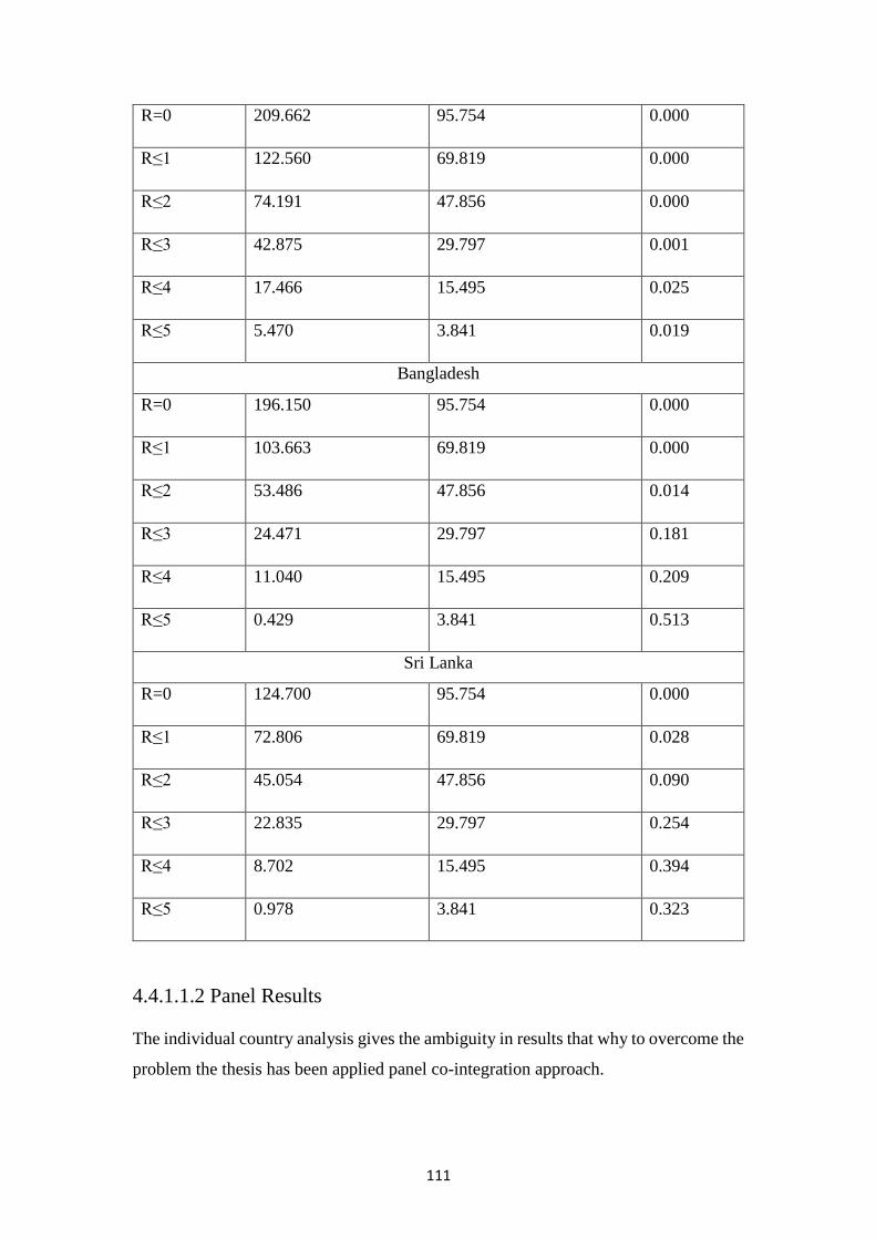
111
R=0 209.662 95.754 0.000
R≤1 122.560 69.819 0.000
R≤2 74.191 47.856 0.000
R≤3 42.875 29.797 0.001
R≤4 17.466 15.495 0.025
R≤5 5.470 3.841 0.019
Bangladesh
R=0 196.150 95.754 0.000
R≤1 103.663 69.819 0.000
R≤2 53.486 47.856 0.014
R≤3 24.471 29.797 0.181
R≤4 11.040 15.495 0.209
R≤5 0.429 3.841 0.513
Sri Lanka
R=0 124.700 95.754 0.000
R≤1 72.806 69.819 0.028
R≤2 45.054 47.856 0.090
R≤3 22.835 29.797 0.254
R≤4 8.702 15.495 0.394
R≤5 0.978 3.841 0.323
4.4.1.1.2 Panel Results
The individual country analysis gives the ambiguity in results that why to overcome the
problem the thesis has been applied panel co-integration approach.
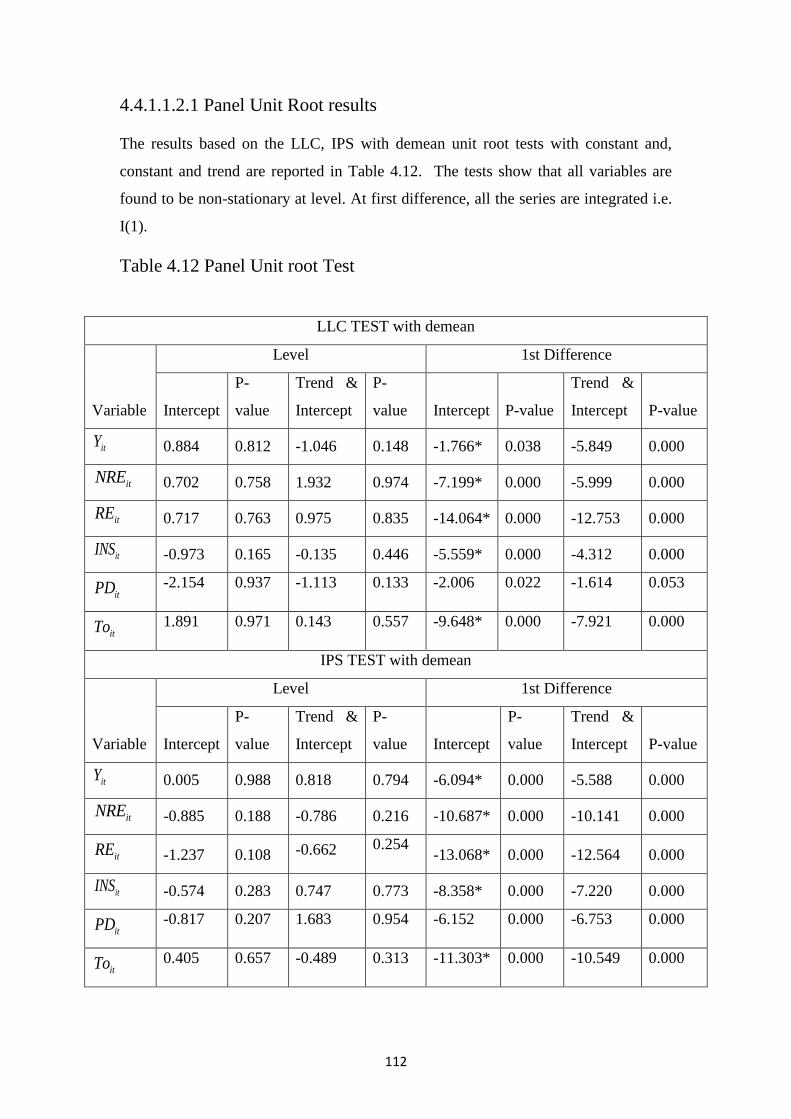
112
4.4.1.1.2.1 Panel Unit Root results
The results based on the LLC, IPS with demean unit root tests with constant and,
constant and trend are reported in Table 4.12. The tests show that all variables are
found to be non-stationary at level. At first difference, all the series are integrated i.e.
I(1).
Table 4.12 Panel Unit root Test
LLC TEST with demean
Variable
Level 1st Difference
Intercept
P-
value
Trend &
Intercept
P-
value Intercept P-value
Trend &
Intercept P-value
itY 0.884 0.812 -1.046 0.148 -1.766* 0.038 -5.849 0.000
itNRE 0.702 0.758 1.932 0.974 -7.199* 0.000 -5.999 0.000
itRE 0.717 0.763 0.975 0.835 -14.064* 0.000 -12.753 0.000
itINS -0.973 0.165 -0.135 0.446 -5.559* 0.000 -4.312 0.000
itPD -2.154 0.937 -1.113 0.133 -2.006 0.022 -1.614 0.053
itTo 1.891 0.971 0.143 0.557 -9.648* 0.000 -7.921 0.000
IPS TEST with demean
Variable
Level 1st Difference
Intercept
P-
value
Trend &
Intercept
P-
value Intercept
P-
value
Trend &
Intercept P-value
itY 0.005 0.988 0.818 0.794 -6.094* 0.000 -5.588 0.000
itNRE -0.885 0.188 -0.786 0.216 -10.687* 0.000 -10.141 0.000
itRE -1.237 0.108 -0.662 0.254 -13.068* 0.000 -12.564 0.000
itINS -0.574 0.283 0.747 0.773 -8.358* 0.000 -7.220 0.000
itPD -0.817 0.207 1.683 0.954 -6.152 0.000 -6.753 0.000
itTo 0.405 0.657 -0.489 0.313 -11.303* 0.000 -10.549 0.000
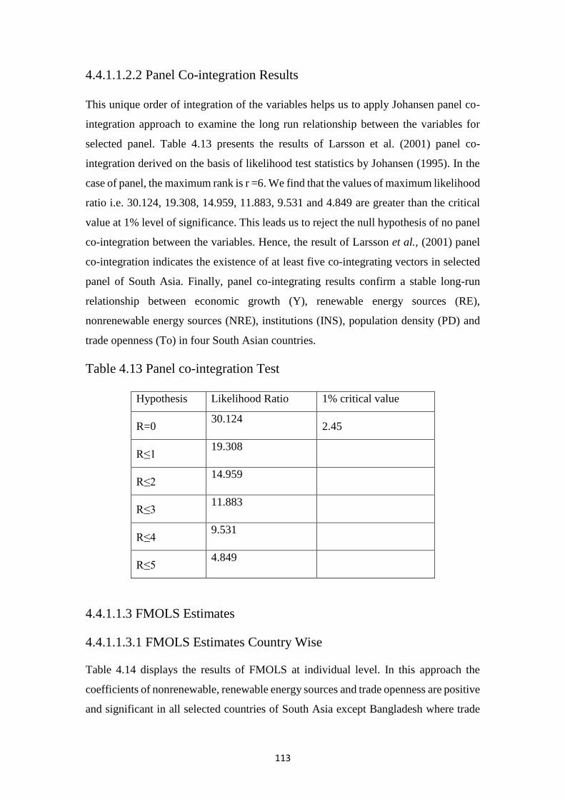
113
4.4.1.1.2.2 Panel Co-integration Results
This unique order of integration of the variables helps us to apply Johansen panel co-
integration approach to examine the long run relationship between the variables for
selected panel. Table 4.13 presents the results of Larsson et al. (2001) panel co-
integration derived on the basis of likelihood test statistics by Johansen (1995). In the
case of panel, the maximum rank is r =6. We find that the values of maximum likelihood
ratio i.e. 30.124, 19.308, 14.959, 11.883, 9.531 and 4.849 are greater than the critical
value at 1% level of significance. This leads us to reject the null hypothesis of no panel
co-integration between the variables. Hence, the result of Larsson et al., (2001) panel
co-integration indicates the existence of at least five co-integrating vectors in selected
panel of South Asia. Finally, panel co-integrating results confirm a stable long-run
relationship between economic growth (Y), renewable energy sources (RE),
nonrenewable energy sources (NRE), institutions (INS), population density (PD) and
trade openness (To) in four South Asian countries.
Table 4.13 Panel co-integration Test
Hypothesis Likelihood Ratio 1% critical value
R=0 30.124
2.45
R≤1 19.308
R≤2 14.959
R≤3 11.883
R≤4 9.531
R≤5 4.849
4.4.1.1.3 FMOLS Estimates
4.4.1.1.3.1 FMOLS Estimates Country Wise
Table 4.14 displays the results of FMOLS at individual level. In this approach the
coefficients of nonrenewable, renewable energy sources and trade openness are positive
and significant in all selected countries of South Asia except Bangladesh where trade
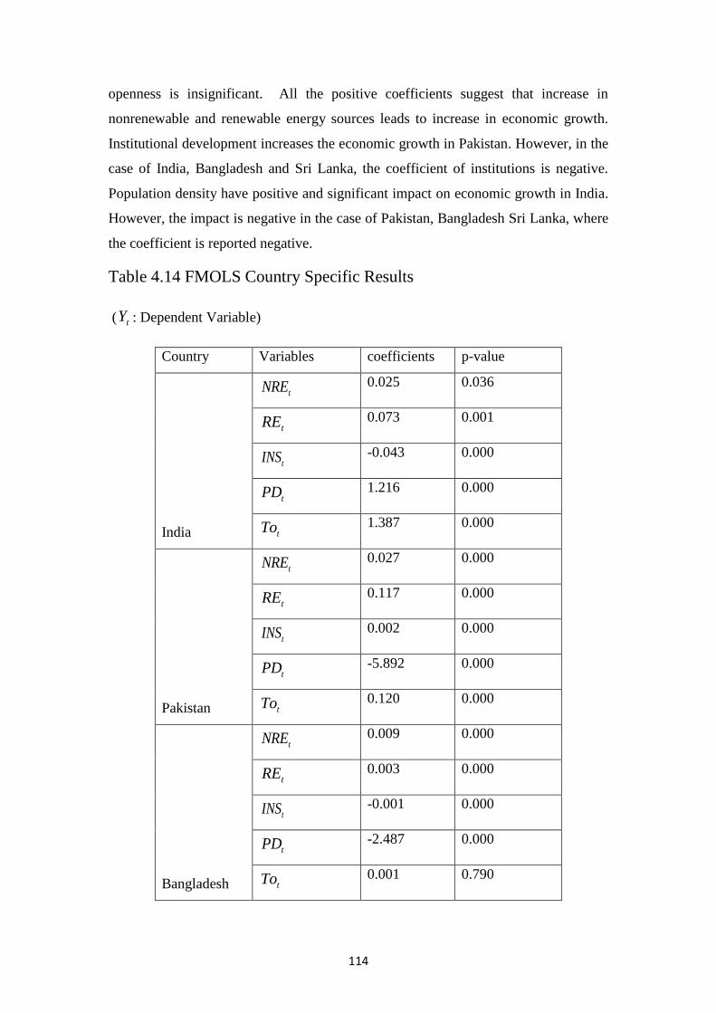
114
openness is insignificant. All the positive coefficients suggest that increase in
nonrenewable and renewable energy sources leads to increase in economic growth.
Institutional development increases the economic growth in Pakistan. However, in the
case of India, Bangladesh and Sri Lanka, the coefficient of institutions is negative.
Population density have positive and significant impact on economic growth in India.
However, the impact is negative in the case of Pakistan, Bangladesh Sri Lanka, where
the coefficient is reported negative.
Table 4.14 FMOLS Country Specific Results
( tY : Dependent Variable)
Country Variables coefficients p-value
India
tNRE 0.025 0.036
tRE 0.073 0.001
tINS -0.043 0.000
tPD 1.216 0.000
tTo 1.387 0.000
Pakistan
tNRE 0.027 0.000
tRE 0.117 0.000
tINS 0.002 0.000
tPD -5.892 0.000
tTo 0.120 0.000
Bangladesh
tNRE 0.009 0.000
tRE 0.003 0.000
tINS -0.001 0.000
tPD -2.487 0.000
tTo 0.001 0.790
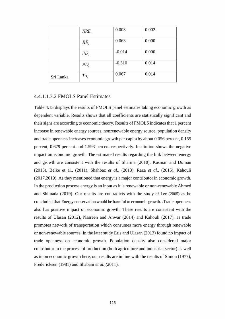
115
Sri Lanka
tNRE 0.003 0.002
tRE 0.063 0.000
tINS -0.014 0.000
tPD -0.310 0.014
tTo 0.067 0.014
4.4.1.1.3.2 FMOLS Panel Estimates
Table 4.15 displays the results of FMOLS panel estimates taking economic growth as
dependent variable. Results shows that all coefficients are statistically significant and
their signs are according to economic theory. Results of FMOLS indicates that 1 percent
increase in renewable energy sources, nonrenewable energy source, population density
and trade openness increases economic growth per capita by about 0.056 percent, 0.159
percent, 0.679 percent and 1.593 percent respectively. Institution shows the negative
impact on economic growth. The estimated results regarding the link between energy
and growth are consistent with the results of Sharma (2010), Kasman and Duman
(2015), Belke et al., (2011), Shahbaz et al., (2013), Raza et al., (2015), Kahouli
(2017,2019). As they mentioned that energy is a major contributor in economic growth.
In the production process energy is an input as it is renewable or non-renewable Ahmed
and Shimada (2019). Our results are contradicts with the study of Lee (2005) as he
concluded that Energy conservation would be harmful to economic growth. .Trade openness
also has positive impact on economic growth. These results are consistent with the
results of Ulasan (2012), Nasreen and Anwar (2014) and Kahouli (2017), as trade
promotes network of transportation which consumes more energy through renewable
or non-renewable sources. In the later study Eris and Ulasan (2013) found no impact of
trade openness on economic growth. Population density also considered major
contributor in the process of production (both agriculture and industrial sector) as well
as in on economic growth here, our results are in line with the results of Simon (1977),
Fredericksen (1981) and Shabani et al.,(2011).
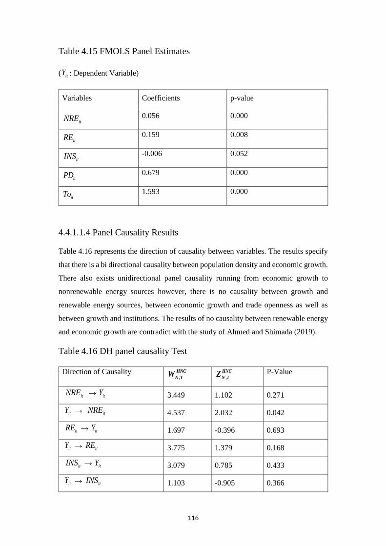
116
Table 4.15 FMOLS Panel Estimates
( itY : Dependent Variable)
Variables Coefficients p-value
itNRE 0.056 0.000
itRE 0.159 0.008
itINS -0.006 0.052
itPD 0.679 0.000
itTo 1.593 0.000
4.4.1.1.4 Panel Causality Results
Table 4.16 represents the direction of causality between variables. The results specify
that there is a bi directional causality between population density and economic growth.
There also exists unidirectional panel causality running from economic growth to
nonrenewable energy sources however, there is no causality between growth and
renewable energy sources, between economic growth and trade openness as well as
between growth and institutions. The results of no causality between renewable energy
and economic growth are contradict with the study of Ahmed and Shimada (2019).
Table 4.16 DH panel causality Test
Direction of Causality ,
HNC
N TW ,
HNC
N TZ P-Value
itNRE → itY 3.449 1.102 0.271
itY → itNRE 4.537 2.032 0.042
itRE → itY 1.697 -0.396 0.693
itY → itRE 3.775 1.379 0.168
itINS → itY 3.079 0.785 0.433
itY → itINS 1.103 -0.905 0.366
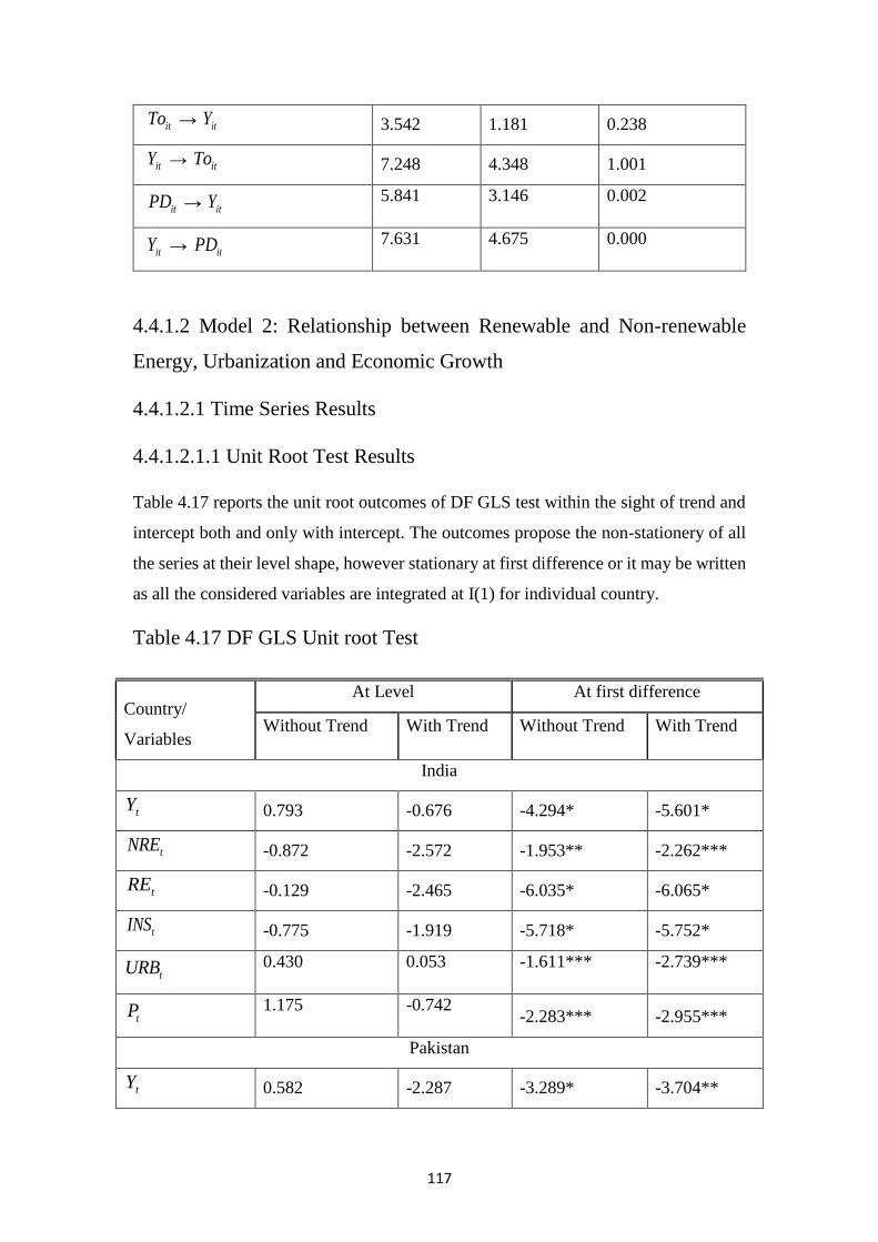
117
itTo → itY 3.542 1.181 0.238
itY → itTo 7.248 4.348 1.001
itPD → itY 5.841 3.146 0.002
itY → itPD 7.631 4.675 0.000
4.4.1.2 Model 2: Relationship between Renewable and Non-renewable
Energy, Urbanization and Economic Growth
4.4.1.2.1 Time Series Results
4.4.1.2.1.1 Unit Root Test Results
Table 4.17 reports the unit root outcomes of DF GLS test within the sight of trend and
intercept both and only with intercept. The outcomes propose the non-stationery of all
the series at their level shape, however stationary at first difference or it may be written
as all the considered variables are integrated at I(1) for individual country.
Table 4.17 DF GLS Unit root Test
Country/
Variables
At Level At first difference
Without Trend With Trend Without Trend With Trend
India
tY 0.793 -0.676 -4.294* -5.601*
tNRE -0.872 -2.572 -1.953** -2.262***
tRE -0.129 -2.465 -6.035* -6.065*
tINS -0.775 -1.919 -5.718* -5.752*
tURB 0.430 0.053 -1.611*** -2.739***
tP 1.175 -0.742
-2.283*** -2.955***
Pakistan
tY 0.582 -2.287 -3.289* -3.704**
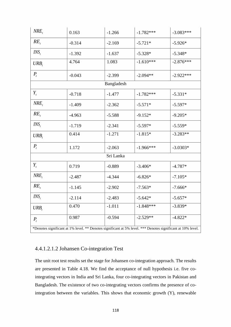
118
4.4.1.2.1.2 Johansen Co-integration Test
The unit root test results set the stage for Johansen co-integration approach. The results
are presented in Table 4.18. We find the acceptance of null hypothesis i.e. five co-
integrating vectors in India and Sri Lanka, four co-integrating vectors in Pakistan and
Bangladesh. The existence of two co-integrating vectors confirms the presence of co-
integration between the variables. This shows that economic growth (Y), renewable
tNRE 0.163 -1.266 -1.782*** -3.083***
tRE -0.314 -2.169 -5.721* -5.926*
tINS -1.392 -1.637 -5.328* -5.348*
tURB 4.764 1.083 -1.610*** -2.876***
tP -0.043 -2.399 -2.094** -2.922***
Bangladesh
tY -0.718 -1.477 -1.782*** -5.331*
tNRE -1.409 -2.362 -5.571* -5.597*
tRE -4.963 -5.588 -9.152* -9.205*
tINS -1.719 -2.341 -5.597* -5.559*
tURB 0.414 -1.271 -1.815* -3.283**
tP 1.172 -2.063 -1.966*** -3.0303*
Sri Lanka
tY 0.719 -0.889 -3.406* -4.787*
tNRE -2.487 -4.344 -6.826* -7.105*
tRE -1.145 -2.902 -7.563* -7.666*
tINS -2.114 -2.483 -5.642* -5.657*
tURB 0.470 -1.011 -1.848*** -3.839*
tP 0.987 -0.594 -2.529** -4.822*
*Denotes significant at 1% level. ** Denotes significant at 5% level. *** Denotes significant at 10% level.
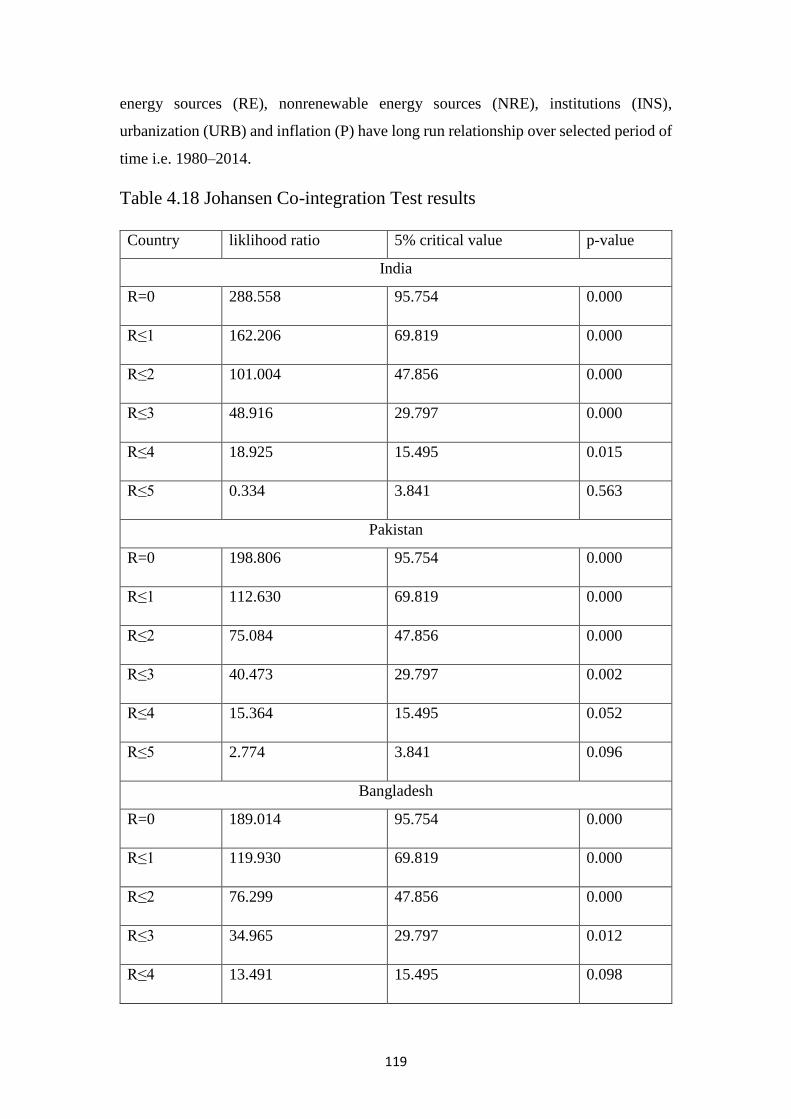
119
energy sources (RE), nonrenewable energy sources (NRE), institutions (INS),
urbanization (URB) and inflation (P) have long run relationship over selected period of
time i.e. 1980–2014.
Table 4.18 Johansen Co-integration Test results
Country liklihood ratio 5% critical value p-value
India
R=0 288.558 95.754 0.000
R≤1 162.206 69.819 0.000
R≤2 101.004 47.856 0.000
R≤3 48.916 29.797 0.000
R≤4 18.925 15.495 0.015
R≤5 0.334 3.841 0.563
Pakistan
R=0 198.806 95.754 0.000
R≤1 112.630 69.819 0.000
R≤2 75.084 47.856 0.000
R≤3 40.473 29.797 0.002
R≤4 15.364 15.495 0.052
R≤5 2.774 3.841 0.096
Bangladesh
R=0 189.014 95.754 0.000
R≤1 119.930 69.819 0.000
R≤2 76.299 47.856 0.000
R≤3 34.965 29.797 0.012
R≤4 13.491 15.495 0.098
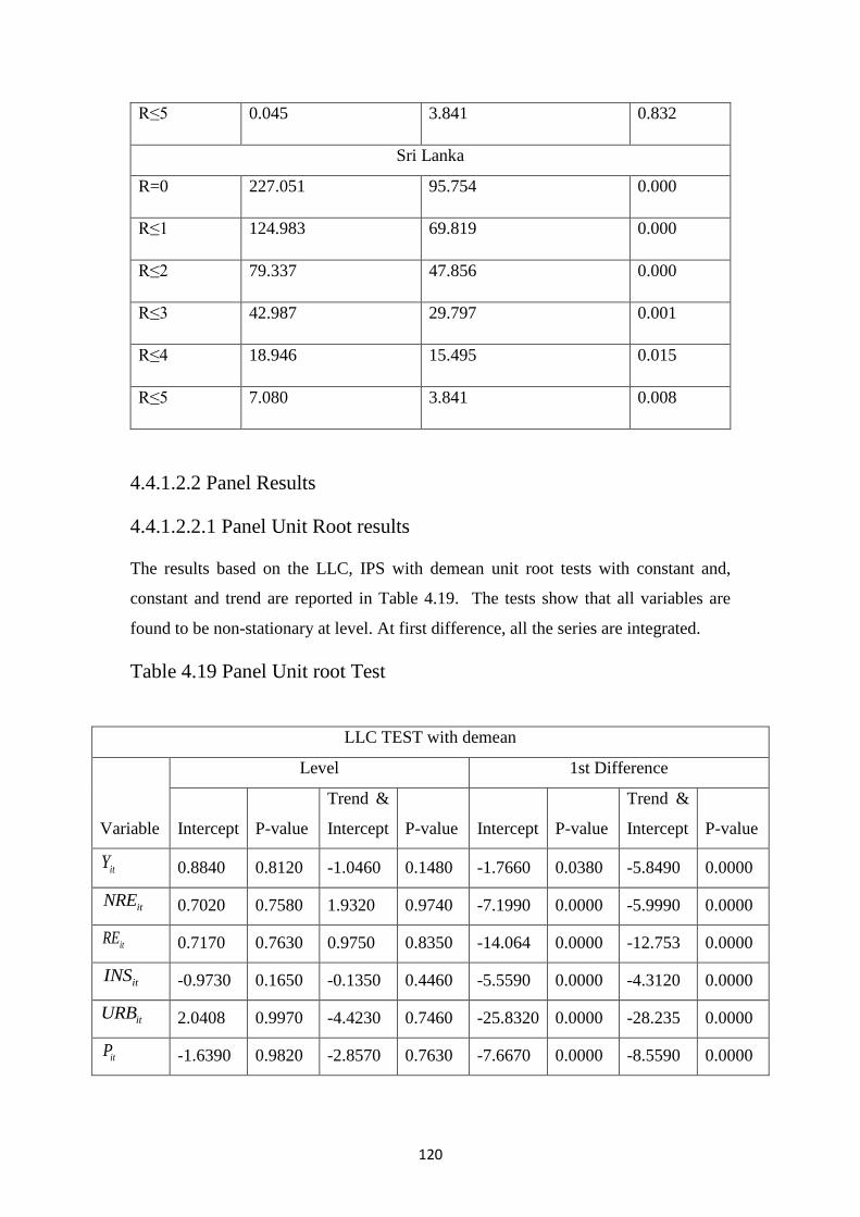
120
R≤5 0.045 3.841 0.832
Sri Lanka
R=0 227.051 95.754 0.000
R≤1 124.983 69.819 0.000
R≤2 79.337 47.856 0.000
R≤3 42.987 29.797 0.001
R≤4 18.946 15.495 0.015
R≤5 7.080 3.841 0.008
4.4.1.2.2 Panel Results
4.4.1.2.2.1 Panel Unit Root results
The results based on the LLC, IPS with demean unit root tests with constant and,
constant and trend are reported in Table 4.19. The tests show that all variables are
found to be non-stationary at level. At first difference, all the series are integrated.
Table 4.19 Panel Unit root Test
LLC TEST with demean
Variable
Level 1st Difference
Intercept P-value
Trend &
Intercept P-value Intercept P-value
Trend &
Intercept P-value
itY 0.8840 0.8120 -1.0460 0.1480 -1.7660 0.0380 -5.8490 0.0000
itNRE 0.7020 0.7580 1.9320 0.9740 -7.1990 0.0000 -5.9990 0.0000
itRE 0.7170 0.7630 0.9750 0.8350 -14.064 0.0000 -12.753 0.0000
itINS -0.9730 0.1650 -0.1350 0.4460 -5.5590 0.0000 -4.3120 0.0000
itURB 2.0408 0.9970 -4.4230 0.7460 -25.8320 0.0000 -28.235 0.0000
itP -1.6390 0.9820 -2.8570 0.7630 -7.6670 0.0000 -8.5590 0.0000
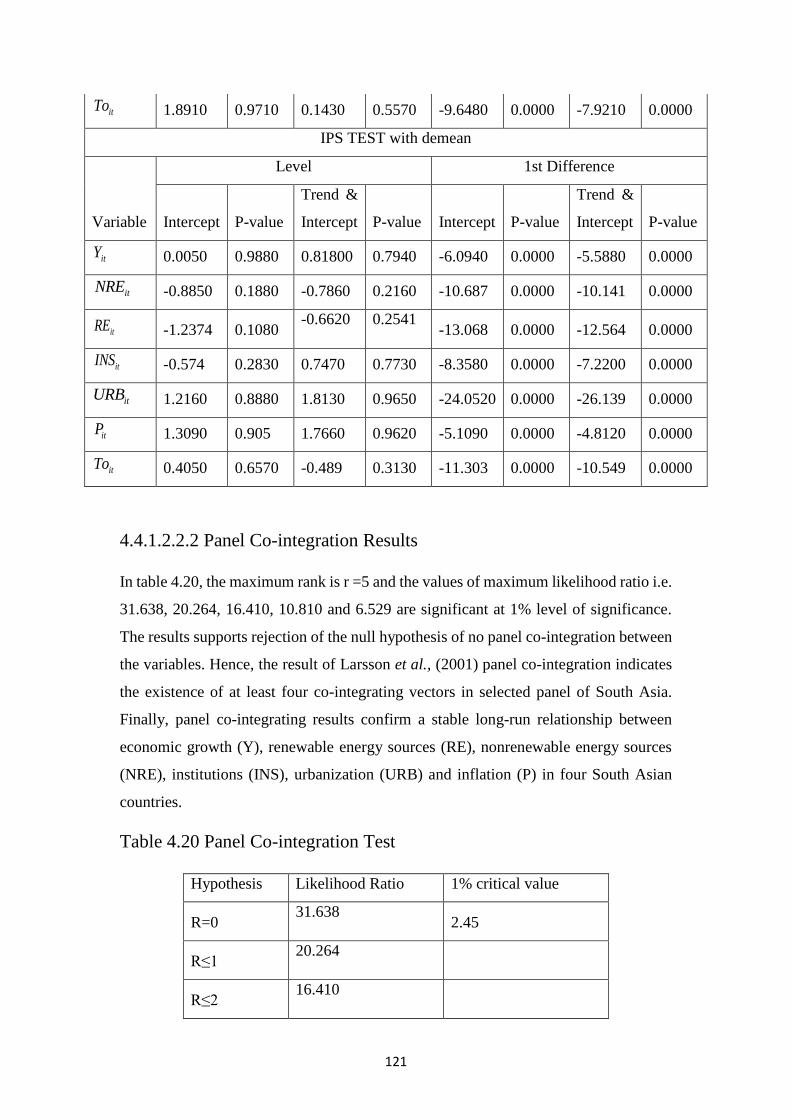
121
4.4.1.2.2.2 Panel Co-integration Results
In table 4.20, the maximum rank is r =5 and the values of maximum likelihood ratio i.e.
31.638, 20.264, 16.410, 10.810 and 6.529 are significant at 1% level of significance.
The results supports rejection of the null hypothesis of no panel co-integration between
the variables. Hence, the result of Larsson et al., (2001) panel co-integration indicates
the existence of at least four co-integrating vectors in selected panel of South Asia.
Finally, panel co-integrating results confirm a stable long-run relationship between
economic growth (Y), renewable energy sources (RE), nonrenewable energy sources
(NRE), institutions (INS), urbanization (URB) and inflation (P) in four South Asian
countries.
Table 4.20 Panel Co-integration Test
Hypothesis Likelihood Ratio 1% critical value
R=0 31.638
2.45
R≤1 20.264
R≤2 16.410
itTo 1.8910 0.9710 0.1430 0.5570 -9.6480 0.0000 -7.9210 0.0000
IPS TEST with demean
Variable
Level 1st Difference
Intercept P-value
Trend &
Intercept P-value Intercept P-value
Trend &
Intercept P-value
itY 0.0050 0.9880 0.81800 0.7940 -6.0940 0.0000 -5.5880 0.0000
itNRE -0.8850 0.1880 -0.7860 0.2160 -10.687 0.0000 -10.141 0.0000
itRE -1.2374 0.1080 -0.6620 0.2541
-13.068 0.0000 -12.564 0.0000
itINS -0.574 0.2830 0.7470 0.7730 -8.3580 0.0000 -7.2200 0.0000
itURB 1.2160 0.8880 1.8130 0.9650 -24.0520 0.0000 -26.139 0.0000
itP 1.3090 0.905 1.7660 0.9620 -5.1090 0.0000 -4.8120 0.0000
itTo 0.4050 0.6570 -0.489 0.3130 -11.303 0.0000 -10.549 0.0000
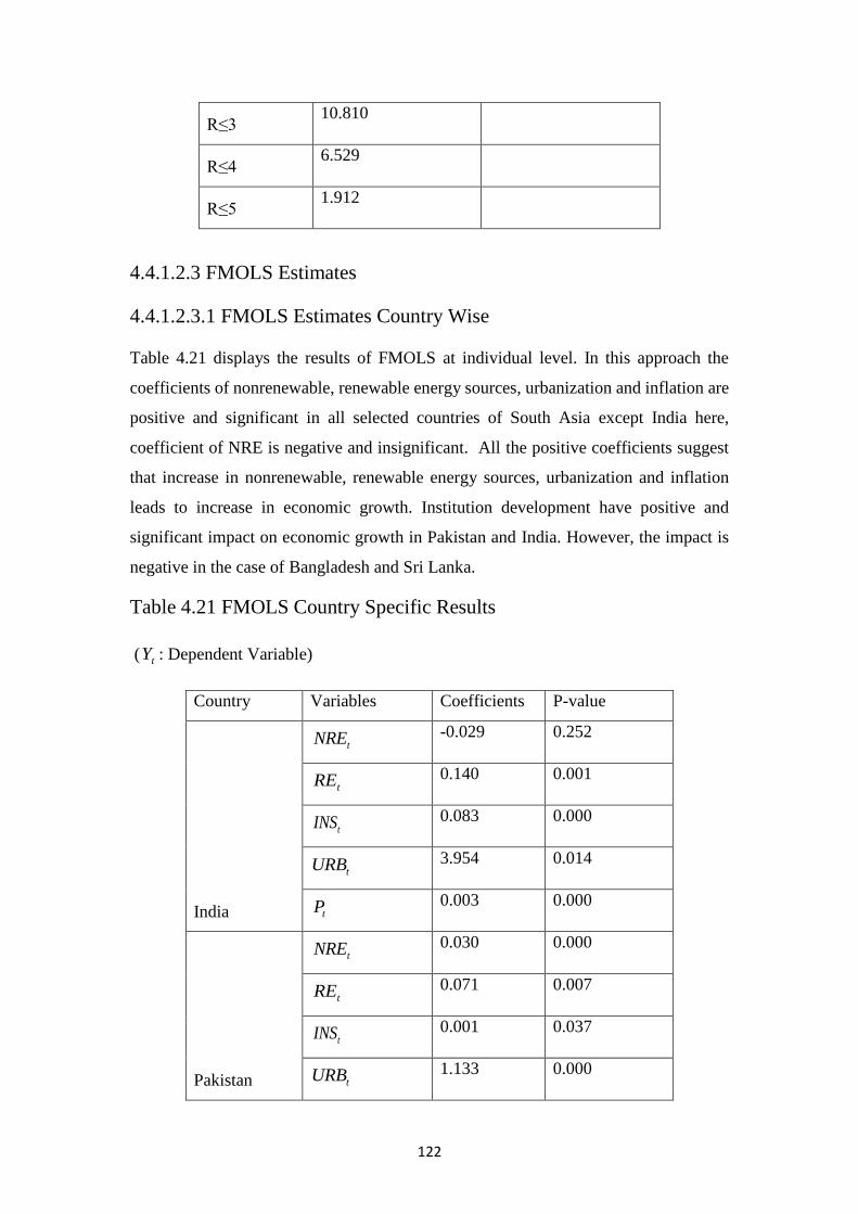
122
R≤3 10.810
R≤4 6.529
R≤5 1.912
4.4.1.2.3 FMOLS Estimates
4.4.1.2.3.1 FMOLS Estimates Country Wise
Table 4.21 displays the results of FMOLS at individual level. In this approach the
coefficients of nonrenewable, renewable energy sources, urbanization and inflation are
positive and significant in all selected countries of South Asia except India here,
coefficient of NRE is negative and insignificant. All the positive coefficients suggest
that increase in nonrenewable, renewable energy sources, urbanization and inflation
leads to increase in economic growth. Institution development have positive and
significant impact on economic growth in Pakistan and India. However, the impact is
negative in the case of Bangladesh and Sri Lanka.
Table 4.21 FMOLS Country Specific Results
( tY : Dependent Variable)
Country Variables Coefficients P-value
India
tNRE -0.029 0.252
tRE 0.140 0.001
tINS 0.083 0.000
tURB 3.954 0.014
tP 0.003 0.000
Pakistan
tNRE 0.030 0.000
tRE 0.071 0.007
tINS 0.001 0.037
tURB 1.133 0.000
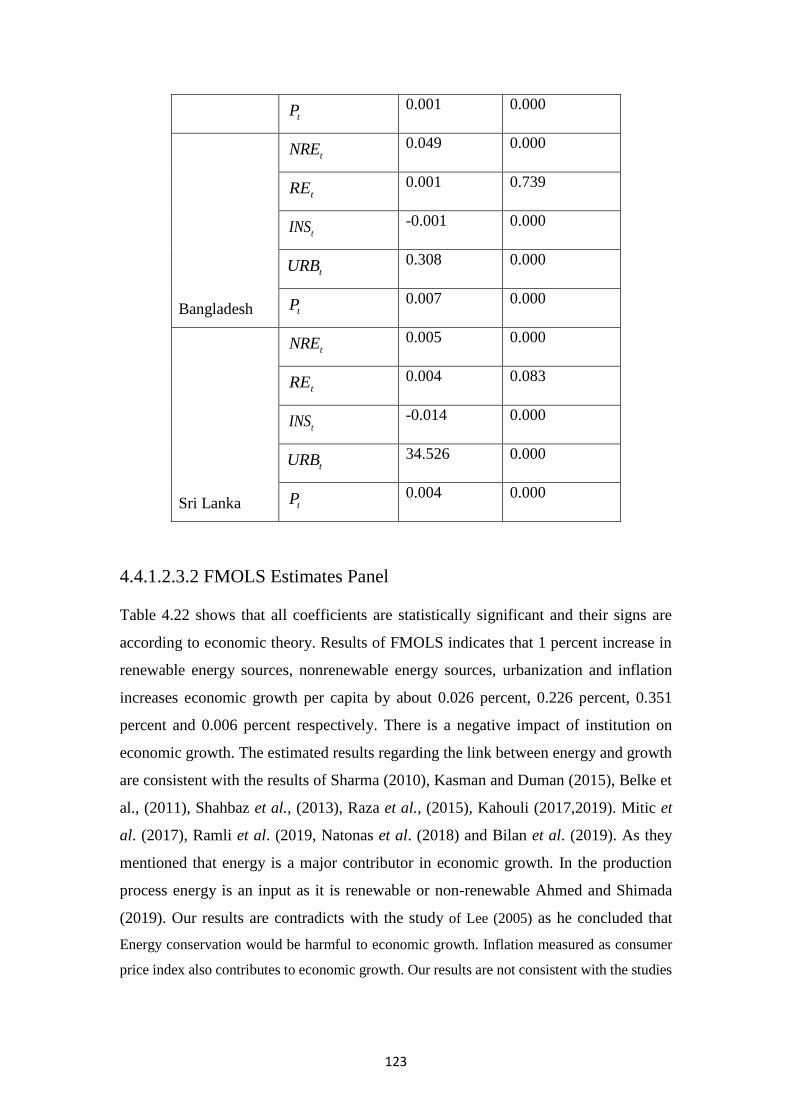
123
tP 0.001 0.000
Bangladesh
tNRE 0.049 0.000
tRE 0.001 0.739
tINS -0.001 0.000
tURB 0.308 0.000
tP 0.007 0.000
Sri Lanka
tNRE 0.005 0.000
tRE 0.004 0.083
tINS -0.014 0.000
tURB 34.526 0.000
tP 0.004 0.000
4.4.1.2.3.2 FMOLS Estimates Panel
Table 4.22 shows that all coefficients are statistically significant and their signs are
according to economic theory. Results of FMOLS indicates that 1 percent increase in
renewable energy sources, nonrenewable energy sources, urbanization and inflation
increases economic growth per capita by about 0.026 percent, 0.226 percent, 0.351
percent and 0.006 percent respectively. There is a negative impact of institution on
economic growth. The estimated results regarding the link between energy and growth
are consistent with the results of Sharma (2010), Kasman and Duman (2015), Belke et
al., (2011), Shahbaz et al., (2013), Raza et al., (2015), Kahouli (2017,2019). Mitic et
al. (2017), Ramli et al. (2019, Natonas et al. (2018) and Bilan et al. (2019). As they
mentioned that energy is a major contributor in economic growth. In the production
process energy is an input as it is renewable or non-renewable Ahmed and Shimada
(2019). Our results are contradicts with the study of Lee (2005) as he concluded that
Energy conservation would be harmful to economic growth. Inflation measured as consumer
price index also contributes to economic growth. Our results are not consistent with the studies
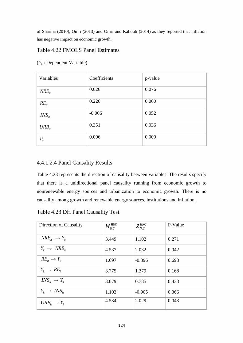
124
of Sharma (2010), Omri (2013) and Omri and Kahouli (2014) as they reported that inflation
has negative impact on economic growth.
Table 4.22 FMOLS Panel Estimates
( itY : Dependent Variable)
Variables Coefficients p-value
itNRE 0.026 0.076
itRE 0.226 0.000
itINS -0.006 0.052
itURB 0.351 0.036
itP 0.006 0.000
4.4.1.2.4 Panel Causality Results
Table 4.23 represents the direction of causality between variables. The results specify
that there is a unidirectional panel causality running from economic growth to
nonrenewable energy sources and urbanization to economic growth. There is no
causality among growth and renewable energy sources, institutions and inflation.
Table 4.23 DH Panel Causality Test
Direction of Causality ,
HNC
N TW ,
HNC
N TZ P-Value
itNRE → itY 3.449 1.102 0.271
itY → itNRE 4.537 2.032 0.042
itRE → itY 1.697 -0.396 0.693
itY → itRE 3.775 1.379 0.168
itINS → itY 3.079 0.785 0.433
itY → itINS 1.103 -0.905 0.366
itURB → itY 4.534 2.029 0.043
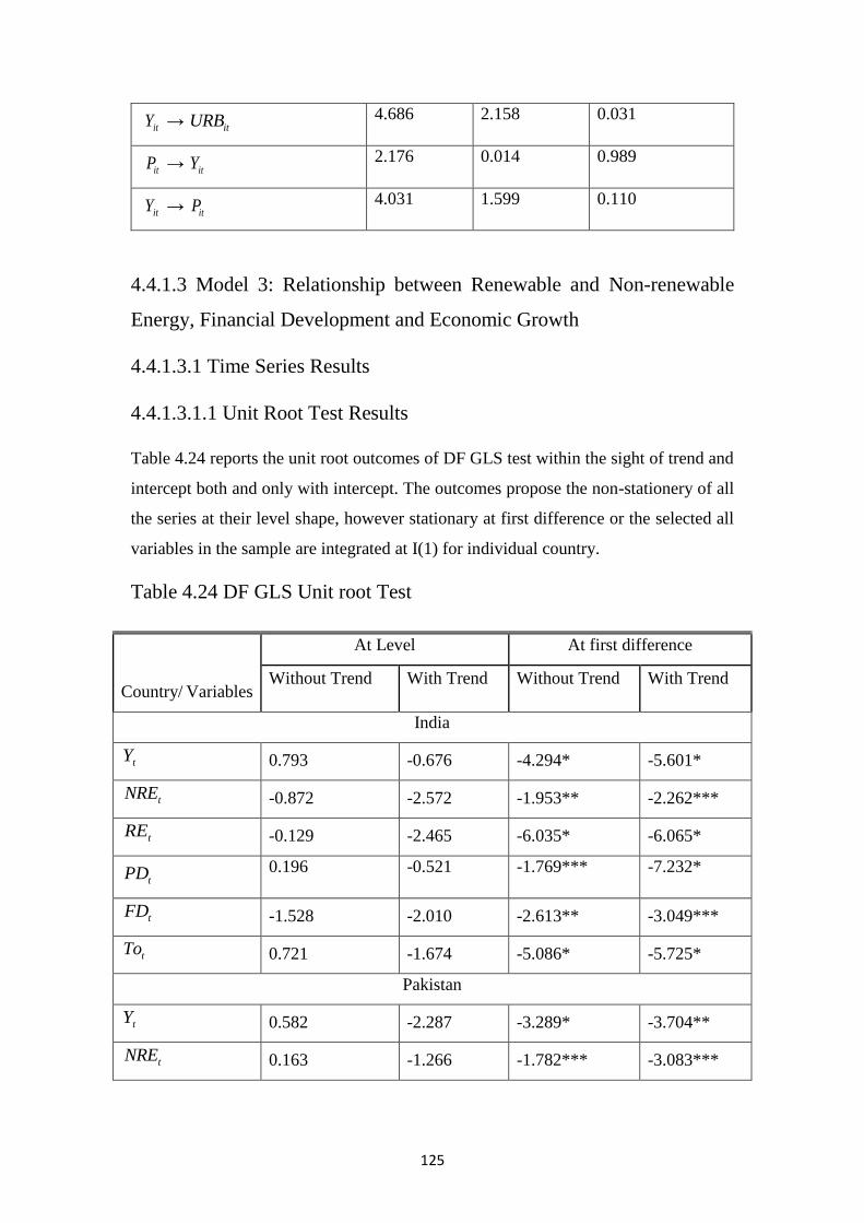
125
itY → itURB 4.686 2.158 0.031
itP → itY 2.176 0.014 0.989
itY → itP 4.031 1.599 0.110
4.4.1.3 Model 3: Relationship between Renewable and Non-renewable
Energy, Financial Development and Economic Growth
4.4.1.3.1 Time Series Results
4.4.1.3.1.1 Unit Root Test Results
Table 4.24 reports the unit root outcomes of DF GLS test within the sight of trend and
intercept both and only with intercept. The outcomes propose the non-stationery of all
the series at their level shape, however stationary at first difference or the selected all
variables in the sample are integrated at I(1) for individual country.
Table 4.24 DF GLS Unit root Test
Country/ Variables
At Level At first difference
Without Trend With Trend Without Trend With Trend
India
tY 0.793 -0.676 -4.294* -5.601*
tNRE -0.872 -2.572 -1.953** -2.262***
tRE -0.129 -2.465 -6.035* -6.065*
tPD 0.196 -0.521 -1.769*** -7.232*
tFD -1.528 -2.010 -2.613** -3.049***
tTo 0.721 -1.674 -5.086* -5.725*
Pakistan
tY 0.582 -2.287 -3.289* -3.704**
tNRE 0.163 -1.266 -1.782*** -3.083***
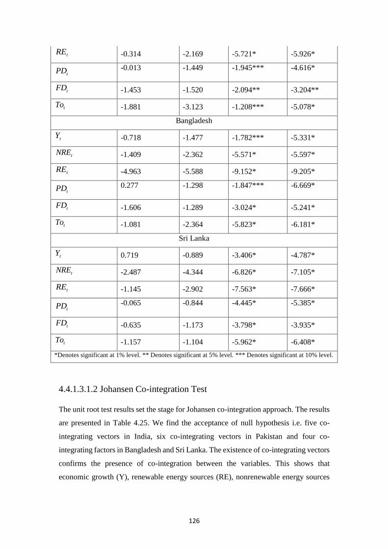
126
4.4.1.3.1.2 Johansen Co-integration Test
The unit root test results set the stage for Johansen co-integration approach. The results
are presented in Table 4.25. We find the acceptance of null hypothesis i.e. five co-
integrating vectors in India, six co-integrating vectors in Pakistan and four co-
integrating factors in Bangladesh and Sri Lanka. The existence of co-integrating vectors
confirms the presence of co-integration between the variables. This shows that
economic growth (Y), renewable energy sources (RE), nonrenewable energy sources
tRE -0.314 -2.169 -5.721* -5.926*
tPD -0.013 -1.449 -1.945*** -4.616*
tFD -1.453 -1.520 -2.094** -3.204**
tTo -1.881 -3.123 -1.208*** -5.078*
Bangladesh
tY -0.718 -1.477 -1.782*** -5.331*
tNRE -1.409 -2.362 -5.571* -5.597*
tRE -4.963 -5.588 -9.152* -9.205*
tPD 0.277 -1.298 -1.847*** -6.669*
tFD -1.606 -1.289 -3.024* -5.241*
tTo -1.081 -2.364 -5.823* -6.181*
Sri Lanka
tY 0.719 -0.889 -3.406* -4.787*
tNRE -2.487 -4.344 -6.826* -7.105*
tRE -1.145 -2.902 -7.563* -7.666*
tPD -0.065 -0.844 -4.445* -5.385*
tFD -0.635 -1.173 -3.798* -3.935*
tTo -1.157 -1.104 -5.962* -6.408*
*Denotes significant at 1% level. ** Denotes significant at 5% level. *** Denotes significant at 10% level.
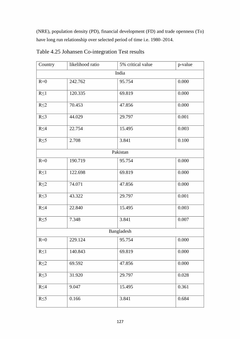
127
(NRE), population density (PD), financial development (FD) and trade openness (To)
have long run relationship over selected period of time i.e. 1980–2014.
Table 4.25 Johansen Co-integration Test results
Country likelihood ratio 5% critical value p-value
India
R=0 242.762 95.754 0.000
R≤1 120.335 69.819 0.000
R≤2 70.453 47.856 0.000
R≤3 44.029 29.797 0.001
R≤4 22.754 15.495 0.003
R≤5 2.708 3.841 0.100
Pakistan
R=0 190.719 95.754 0.000
R≤1 122.698 69.819 0.000
R≤2 74.071 47.856 0.000
R≤3 43.322 29.797 0.001
R≤4 22.840 15.495 0.003
R≤5 7.348 3.841 0.007
Bangladesh
R=0 229.124 95.754 0.000
R≤1 140.843 69.819 0.000
R≤2 69.592 47.856 0.000
R≤3 31.920 29.797 0.028
R≤4 9.047 15.495 0.361
R≤5 0.166 3.841 0.684
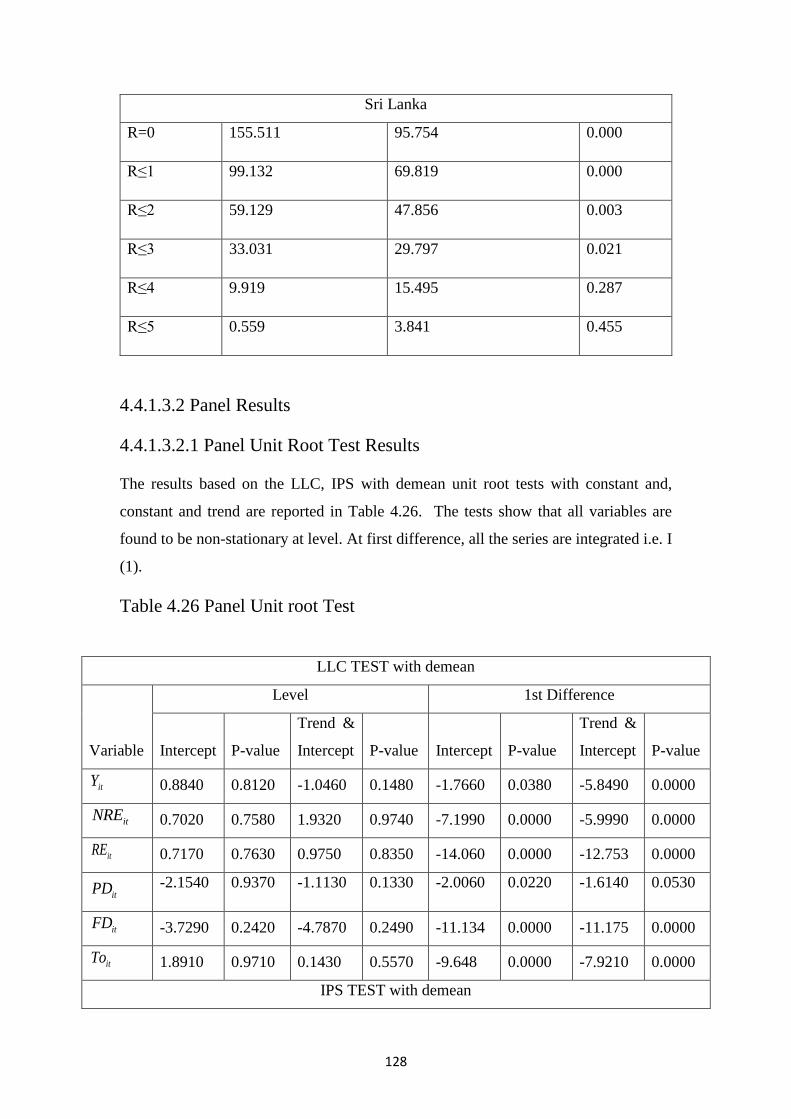
128
Sri Lanka
R=0 155.511 95.754 0.000
R≤1 99.132 69.819 0.000
R≤2 59.129 47.856 0.003
R≤3 33.031 29.797 0.021
R≤4 9.919 15.495 0.287
R≤5 0.559 3.841 0.455
4.4.1.3.2 Panel Results
4.4.1.3.2.1 Panel Unit Root Test Results
The results based on the LLC, IPS with demean unit root tests with constant and,
constant and trend are reported in Table 4.26. The tests show that all variables are
found to be non-stationary at level. At first difference, all the series are integrated i.e. I
(1).
Table 4.26 Panel Unit root Test
LLC TEST with demean
Variable
Level 1st Difference
Intercept P-value
Trend &
Intercept P-value Intercept P-value
Trend &
Intercept P-value
itY 0.8840 0.8120 -1.0460 0.1480 -1.7660 0.0380 -5.8490 0.0000
itNRE 0.7020 0.7580 1.9320 0.9740 -7.1990 0.0000 -5.9990 0.0000
itRE 0.7170 0.7630 0.9750 0.8350 -14.060 0.0000 -12.753 0.0000
itPD -2.1540 0.9370 -1.1130 0.1330 -2.0060 0.0220 -1.6140 0.0530
itFD -3.7290 0.2420 -4.7870 0.2490 -11.134 0.0000 -11.175 0.0000
itTo 1.8910 0.9710 0.1430 0.5570 -9.648 0.0000 -7.9210 0.0000
IPS TEST with demean
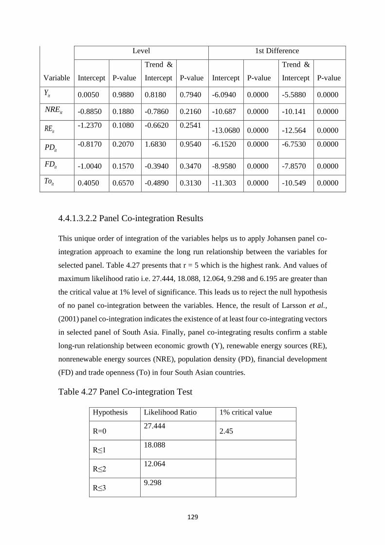
129
4.4.1.3.2.2 Panel Co-integration Results
This unique order of integration of the variables helps us to apply Johansen panel co-
integration approach to examine the long run relationship between the variables for
selected panel. Table 4.27 presents that r = 5 which is the highest rank. And values of
maximum likelihood ratio i.e. 27.444, 18.088, 12.064, 9.298 and 6.195 are greater than
the critical value at 1% level of significance. This leads us to reject the null hypothesis
of no panel co-integration between the variables. Hence, the result of Larsson et al.,
(2001) panel co-integration indicates the existence of at least four co-integrating vectors
in selected panel of South Asia. Finally, panel co-integrating results confirm a stable
long-run relationship between economic growth (Y), renewable energy sources (RE),
nonrenewable energy sources (NRE), population density (PD), financial development
(FD) and trade openness (To) in four South Asian countries.
Table 4.27 Panel Co-integration Test
Hypothesis Likelihood Ratio 1% critical value
R=0 27.444
2.45
R≤1 18.088
R≤2 12.064
R≤3 9.298
Variable
Level 1st Difference
Intercept P-value
Trend &
Intercept P-value Intercept P-value
Trend &
Intercept P-value
itY 0.0050 0.9880 0.8180 0.7940 -6.0940 0.0000 -5.5880 0.0000
itNRE -0.8850 0.1880 -0.7860 0.2160 -10.687 0.0000 -10.141 0.0000
itRE -1.2370 0.1080 -0.6620 0.2541
-13.0680 0.0000 -12.564 0.0000
itPD -0.8170 0.2070 1.6830 0.9540 -6.1520 0.0000 -6.7530 0.0000
itFD -1.0040 0.1570 -0.3940 0.3470 -8.9580 0.0000 -7.8570 0.0000
itTo 0.4050 0.6570 -0.4890 0.3130 -11.303 0.0000 -10.549 0.0000
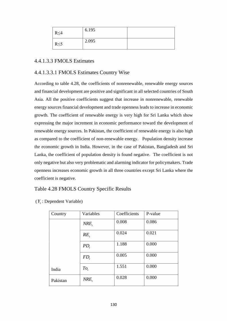
130
R≤4 6.195
R≤5 2.095
4.4.1.3.3 FMOLS Estimates
4.4.1.3.3.1 FMOLS Estimates Country Wise
According to table 4.28, the coefficients of nonrenewable, renewable energy sources
and financial development are positive and significant in all selected countries of South
Asia. All the positive coefficients suggest that increase in nonrenewable, renewable
energy sources financial development and trade openness leads to increase in economic
growth. The coefficient of renewable energy is very high for Sri Lanka which show
expressing the major increment in economic performance toward the development of
renewable energy sources. In Pakistan, the coefficient of renewable energy is also high
as compared to the coefficient of non-renewable energy. Population density increase
the economic growth in India. However, in the case of Pakistan, Bangladesh and Sri
Lanka, the coefficient of population density is found negative. The coefficient is not
only negative but also very problematic and alarming indicator for policymakers. Trade
openness increases economic growth in all three countries except Sri Lanka where the
coefficient is negative.
Table 4.28 FMOLS Country Specific Results
( tY : Dependent Variable)
Country Variables Coefficients P-value
India
tNRE 0.008 0.086
tRE 0.024 0.021
tPD 1.188 0.000
tFD 0.005 0.000
tTo 1.551 0.000
Pakistan tNRE 0.028 0.000
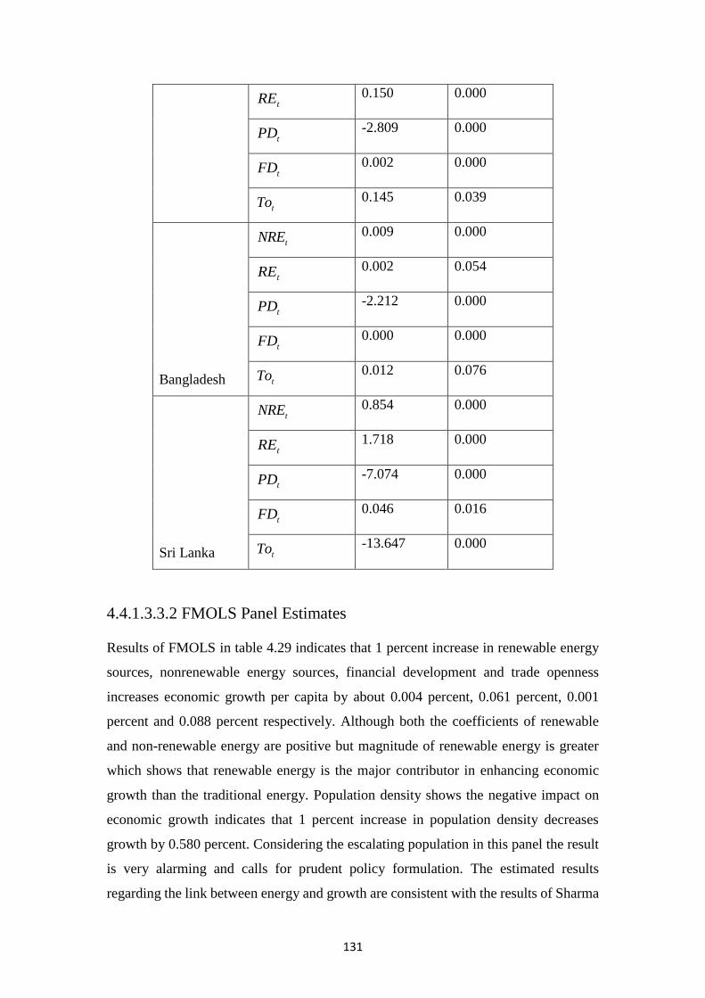
131
tRE 0.150 0.000
tPD -2.809 0.000
tFD 0.002 0.000
tTo 0.145 0.039
Bangladesh
tNRE 0.009 0.000
tRE 0.002 0.054
tPD -2.212 0.000
tFD 0.000 0.000
tTo 0.012 0.076
Sri Lanka
tNRE 0.854 0.000
tRE 1.718 0.000
tPD -7.074 0.000
tFD 0.046 0.016
tTo -13.647 0.000
4.4.1.3.3.2 FMOLS Panel Estimates
Results of FMOLS in table 4.29 indicates that 1 percent increase in renewable energy
sources, nonrenewable energy sources, financial development and trade openness
increases economic growth per capita by about 0.004 percent, 0.061 percent, 0.001
percent and 0.088 percent respectively. Although both the coefficients of renewable
and non-renewable energy are positive but magnitude of renewable energy is greater
which shows that renewable energy is the major contributor in enhancing economic
growth than the traditional energy. Population density shows the negative impact on
economic growth indicates that 1 percent increase in population density decreases
growth by 0.580 percent. Considering the escalating population in this panel the result
is very alarming and calls for prudent policy formulation. The estimated results
regarding the link between energy and growth are consistent with the results of Sharma
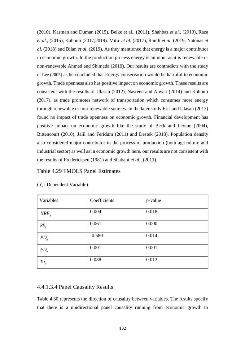
132
(2010), Kasman and Duman (2015), Belke et al., (2011), Shahbaz et al., (2013), Raza
et al., (2015), Kahouli (2017,2019). Mitic et al. (2017), Ramli et al. (2019, Natonas et
al. (2018) and Bilan et al. (2019). As they mentioned that energy is a major contributor
in economic growth. In the production process energy is an input as it is renewable or
non-renewable Ahmed and Shimada (2019). Our results are contradicts with the study
of Lee (2005) as he concluded that Energy conservation would be harmful to economic
growth. Trade openness also has positive impact on economic growth. These results are
consistent with the results of Ulasan (2012), Nasreen and Anwar (2014) and Kahouli
(2017), as trade promotes network of transportation which consumes more energy
through renewable or non-renewable sources. In the later study Eris and Ulasan (2013)
found no impact of trade openness on economic growth. Financial development has
positive impact on economic growth like the study of Beck and Levine (2004),
Bittencourt (2010), Jalil and Feridum (2011) and Destek (2018). Population density
also considered major contributor in the process of production (both agriculture and
industrial sector) as well as in economic growth here, our results are not consistent with
the results of Fredericksen (1981) and Shabani et al., (2011).
Table 4.29 FMOLS Panel Estimates
( itY : Dependent Variable)
Variables Coefficients p-value
itNRE 0.004 0.018
itRE 0.061 0.000
itPD -0.580 0.014
itFD 0.001 0.001
itTo 0.088 0.013
4.4.1.3.4 Panel Causality Results
Table 4.30 represents the direction of causality between variables. The results specify
that there is a unidirectional panel causality running from economic growth to
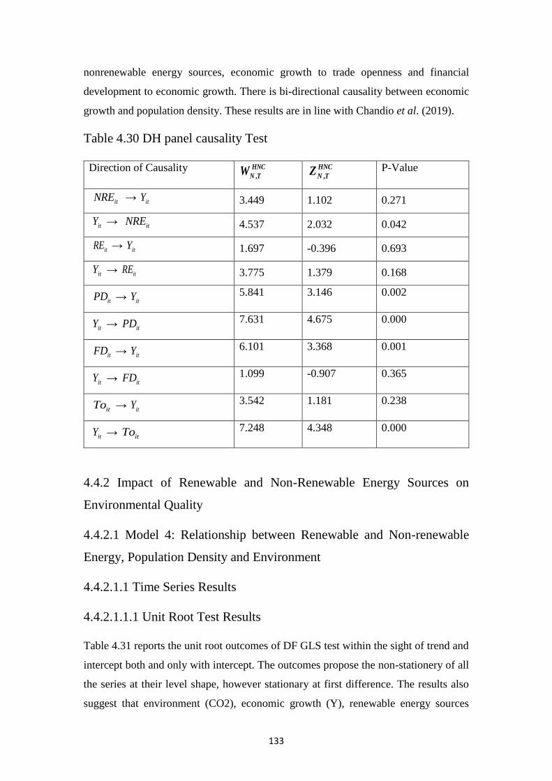
133
nonrenewable energy sources, economic growth to trade openness and financial
development to economic growth. There is bi-directional causality between economic
growth and population density. These results are in line with Chandio et al. (2019).
Table 4.30 DH panel causality Test
Direction of Causality ,
HNC
N TW ,
HNC
N TZ P-Value
itNRE → itY 3.449 1.102 0.271
itY → itNRE 4.537 2.032 0.042
itRE → itY 1.697 -0.396 0.693
itY → itRE 3.775 1.379 0.168
itPD → itY 5.841 3.146 0.002
itY → itPD 7.631 4.675 0.000
itFD → itY 6.101 3.368 0.001
itY → itFD 1.099 -0.907 0.365
itTo → itY 3.542 1.181 0.238
itY → itTo 7.248 4.348 0.000
4.4.2 Impact of Renewable and Non-Renewable Energy Sources on
Environmental Quality
4.4.2.1 Model 4: Relationship between Renewable and Non-renewable
Energy, Population Density and Environment
4.4.2.1.1 Time Series Results
4.4.2.1.1.1 Unit Root Test Results
Table 4.31 reports the unit root outcomes of DF GLS test within the sight of trend and
intercept both and only with intercept. The outcomes propose the non-stationery of all
the series at their level shape, however stationary at first difference. The results also
suggest that environment (CO2), economic growth (Y), renewable energy sources
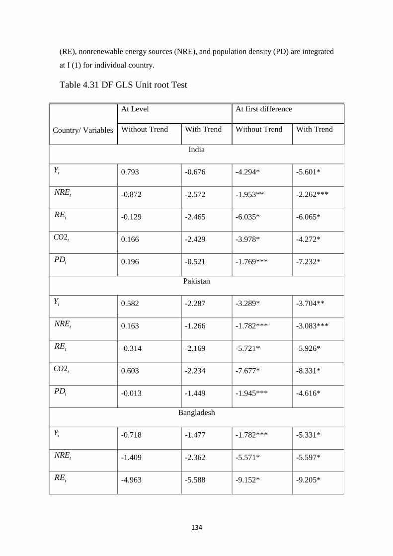
134
(RE), nonrenewable energy sources (NRE), and population density (PD) are integrated
at I (1) for individual country.
Table 4.31 DF GLS Unit root Test
Country/ Variables
At Level At first difference
Without Trend With Trend Without Trend With Trend
India
tY 0.793 -0.676 -4.294* -5.601*
tNRE -0.872 -2.572 -1.953** -2.262***
tRE -0.129 -2.465 -6.035* -6.065*
2tCO 0.166 -2.429 -3.978* -4.272*
tPD 0.196 -0.521 -1.769*** -7.232*
Pakistan
tY 0.582 -2.287 -3.289* -3.704**
tNRE 0.163 -1.266 -1.782*** -3.083***
tRE -0.314 -2.169 -5.721* -5.926*
2tCO 0.603 -2.234 -7.677* -8.331*
tPD -0.013 -1.449 -1.945*** -4.616*
Bangladesh
tY -0.718 -1.477 -1.782*** -5.331*
tNRE -1.409 -2.362 -5.571* -5.597*
tRE -4.963 -5.588 -9.152* -9.205*
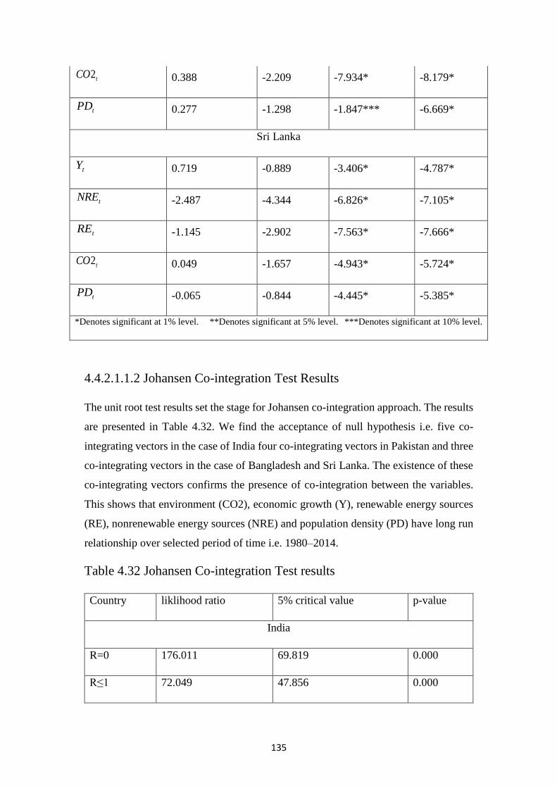
135
4.4.2.1.1.2 Johansen Co-integration Test Results
The unit root test results set the stage for Johansen co-integration approach. The results
are presented in Table 4.32. We find the acceptance of null hypothesis i.e. five co-
integrating vectors in the case of India four co-integrating vectors in Pakistan and three
co-integrating vectors in the case of Bangladesh and Sri Lanka. The existence of these
co-integrating vectors confirms the presence of co-integration between the variables.
This shows that environment (CO2), economic growth (Y), renewable energy sources
(RE), nonrenewable energy sources (NRE) and population density (PD) have long run
relationship over selected period of time i.e. 1980–2014.
Table 4.32 Johansen Co-integration Test results
Country liklihood ratio 5% critical value p-value
India
R=0 176.011 69.819 0.000
R≤1 72.049 47.856 0.000
2tCO 0.388 -2.209 -7.934* -8.179*
tPD 0.277 -1.298 -1.847*** -6.669*
Sri Lanka
tY 0.719 -0.889 -3.406* -4.787*
tNRE -2.487 -4.344 -6.826* -7.105*
tRE -1.145 -2.902 -7.563* -7.666*
2tCO 0.049 -1.657 -4.943* -5.724*
tPD -0.065 -0.844 -4.445* -5.385*
*Denotes significant at 1% level. **Denotes significant at 5% level. ***Denotes significant at 10% level.
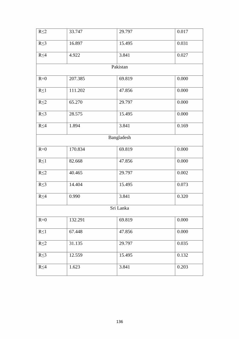
136
R≤2 33.747 29.797 0.017
R≤3 16.897 15.495 0.031
R≤4 4.922 3.841 0.027
Pakistan
R=0 207.385 69.819 0.000
R≤1 111.202 47.856 0.000
R≤2 65.270 29.797 0.000
R≤3 28.575 15.495 0.000
R≤4 1.894 3.841 0.169
Bangladesh
R=0 170.834 69.819 0.000
R≤1 82.668 47.856 0.000
R≤2 40.465 29.797 0.002
R≤3 14.404 15.495 0.073
R≤4 0.990 3.841 0.320
Sri Lanka
R=0 132.291 69.819 0.000
R≤1 67.448 47.856 0.000
R≤2 31.135 29.797 0.035
R≤3 12.559 15.495 0.132
R≤4 1.623 3.841 0.203
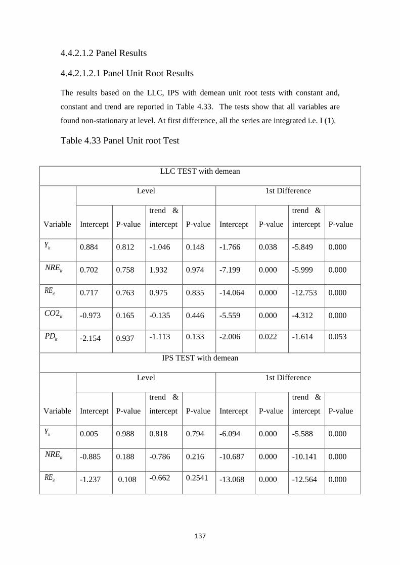
137
4.4.2.1.2 Panel Results
4.4.2.1.2.1 Panel Unit Root Results
The results based on the LLC, IPS with demean unit root tests with constant and,
constant and trend are reported in Table 4.33. The tests show that all variables are
found non-stationary at level. At first difference, all the series are integrated i.e. I (1).
Table 4.33 Panel Unit root Test
LLC TEST with demean
Variable
Level 1st Difference
Intercept P-value
trend &
intercept P-value Intercept P-value
trend &
intercept P-value
itY 0.884 0.812 -1.046 0.148 -1.766 0.038 -5.849 0.000
itNRE 0.702 0.758 1.932 0.974 -7.199 0.000 -5.999 0.000
itRE 0.717 0.763 0.975 0.835 -14.064 0.000 -12.753 0.000
2itCO -0.973 0.165 -0.135 0.446 -5.559 0.000 -4.312 0.000
itPD -2.154 0.937 -1.113 0.133 -2.006 0.022 -1.614 0.053
IPS TEST with demean
Variable
Level 1st Difference
Intercept P-value
trend &
intercept P-value Intercept P-value
trend &
intercept P-value
itY 0.005 0.988 0.818 0.794 -6.094 0.000 -5.588 0.000
itNRE -0.885 0.188 -0.786 0.216 -10.687 0.000 -10.141 0.000
itRE -1.237 0.108 -0.662 0.2541 -13.068 0.000 -12.564 0.000
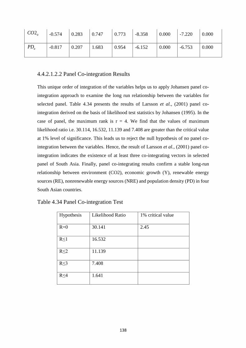
138
4.4.2.1.2.2 Panel Co-integration Results
This unique order of integration of the variables helps us to apply Johansen panel co-
integration approach to examine the long run relationship between the variables for
selected panel. Table 4.34 presents the results of Larsson et al., (2001) panel co-
integration derived on the basis of likelihood test statistics by Johansen (1995). In the
case of panel, the maximum rank is r = 4. We find that the values of maximum
likelihood ratio i.e. 30.114, 16.532, 11.139 and 7.408 are greater than the critical value
at 1% level of significance. This leads us to reject the null hypothesis of no panel co-
integration between the variables. Hence, the result of Larsson et al., (2001) panel co-
integration indicates the existence of at least three co-integrating vectors in selected
panel of South Asia. Finally, panel co-integrating results confirm a stable long-run
relationship between environment (CO2), economic growth (Y), renewable energy
sources (RE), nonrenewable energy sources (NRE) and population density (PD) in four
South Asian countries.
Table 4.34 Panel Co-integration Test
Hypothesis Likelihood Ratio 1% critical value
R=0 30.141 2.45
R≤1 16.532
R≤2 11.139
R≤3 7.408
R≤4 1.641
2itCO -0.574 0.283 0.747 0.773 -8.358 0.000 -7.220 0.000
itPD -0.817 0.207 1.683 0.954 -6.152 0.000 -6.753 0.000
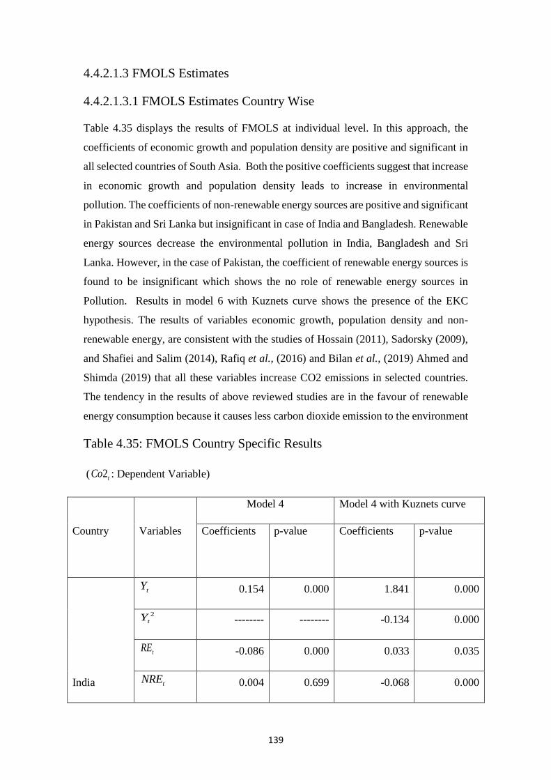
139
4.4.2.1.3 FMOLS Estimates
4.4.2.1.3.1 FMOLS Estimates Country Wise
Table 4.35 displays the results of FMOLS at individual level. In this approach, the
coefficients of economic growth and population density are positive and significant in
all selected countries of South Asia. Both the positive coefficients suggest that increase
in economic growth and population density leads to increase in environmental
pollution. The coefficients of non-renewable energy sources are positive and significant
in Pakistan and Sri Lanka but insignificant in case of India and Bangladesh. Renewable
energy sources decrease the environmental pollution in India, Bangladesh and Sri
Lanka. However, in the case of Pakistan, the coefficient of renewable energy sources is
found to be insignificant which shows the no role of renewable energy sources in
Pollution. Results in model 6 with Kuznets curve shows the presence of the EKC
hypothesis. The results of variables economic growth, population density and non-
renewable energy, are consistent with the studies of Hossain (2011), Sadorsky (2009),
and Shafiei and Salim (2014), Rafiq et al., (2016) and Bilan et al., (2019) Ahmed and
Shimda (2019) that all these variables increase CO2 emissions in selected countries.
The tendency in the results of above reviewed studies are in the favour of renewable
energy consumption because it causes less carbon dioxide emission to the environment
Table 4.35: FMOLS Country Specific Results
( 2tCo : Dependent Variable)
Country
Variables
Model 4 Model 4 with Kuznets curve
Coefficients
p-value
Coefficients
p-value
India
tY 0.154 0.000 1.841 0.000
2
tY -------- -------- -0.134 0.000
tRE -0.086 0.000 0.033 0.035
tNRE 0.004 0.699 -0.068 0.000
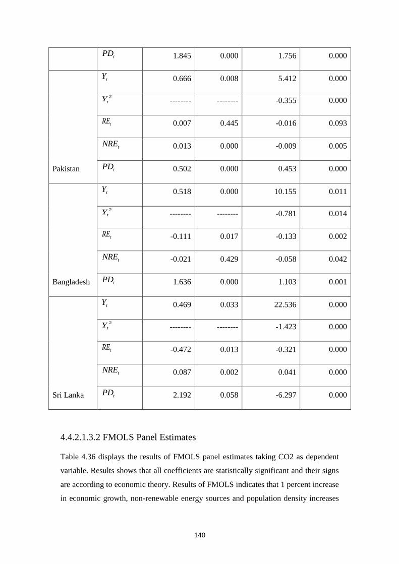
140
tPD 1.845 0.000 1.756 0.000
Pakistan
tY 0.666 0.008 5.412 0.000
2
tY -------- -------- -0.355 0.000
tRE 0.007 0.445 -0.016 0.093
tNRE 0.013 0.000 -0.009 0.005
tPD 0.502 0.000 0.453 0.000
Bangladesh
tY 0.518 0.000 10.155 0.011
2
tY -------- -------- -0.781 0.014
tRE -0.111 0.017 -0.133 0.002
tNRE -0.021 0.429 -0.058 0.042
tPD 1.636 0.000 1.103 0.001
Sri Lanka
tY 0.469 0.033 22.536 0.000
2
tY -------- -------- -1.423 0.000
tRE -0.472 0.013 -0.321 0.000
tNRE 0.087 0.002 0.041 0.000
tPD 2.192 0.058 -6.297 0.000
4.4.2.1.3.2 FMOLS Panel Estimates
Table 4.36 displays the results of FMOLS panel estimates taking CO2 as dependent
variable. Results shows that all coefficients are statistically significant and their signs
are according to economic theory. Results of FMOLS indicates that 1 percent increase
in economic growth, non-renewable energy sources and population density increases
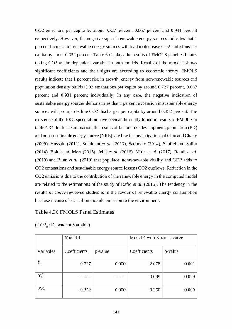
141
CO2 emissions per capita by about 0.727 percent, 0.067 percent and 0.931 percent
respectively. However, the negative sign of renewable energy sources indicates that 1
percent increase in renewable energy sources will lead to decrease CO2 emissions per
capita by about 0.352 percent. Table 6 displays the results of FMOLS panel estimates
taking CO2 as the dependent variable in both models. Results of the model I shows
significant coefficients and their signs are according to economic theory. FMOLS
results indicate that 1 percent rise in growth, energy from non-renewable sources and
population density builds CO2 emanations per capita by around 0.727 percent, 0.067
percent and 0.931 percent individually. In any case, the negative indication of
sustainable energy sources demonstrates that 1 percent expansion in sustainable energy
sources will prompt decline CO2 discharges per capita by around 0.352 percent. The
existence of the EKC speculation have been additionally found in results of FMOLS in
table 4.34. In this examination, the results of factors like development, population (PD)
and non-sustainable energy source (NRE), are like the investigations of Chiu and Chang
(2009), Hossain (2011), Sulaiman et al. (2013), Sadorsky (2014), Shafiei and Salim
(2014), Boluk and Mert (2015), Jebli et al. (2016), Mitic et al. (2017), Ramli et al.
(2019) and Bilan et al. (2019) that populace, nonrenewable vitality and GDP adds to
CO2 emanations and sustainable energy source lessens CO2 outflows. Reduction in the
CO2 emissions due to the contribution of the renewable energy in the computed model
are related to the estimations of the study of Rafiq et al. (2016). The tendency in the
results of above-reviewed studies is in the favour of renewable energy consumption
because it causes less carbon dioxide emission to the environment.
Table 4.36 FMOLS Panel Estimates
( 2itCO : Dependent Variable)
Variables
Model 4 Model 4 with Kuznets curve
Coefficients p-value Coefficients p-value
itY 0.727 0.000 2.078 0.001
2
itY -------- -------- -0.099 0.029
itRE -0.352 0.000 -0.250 0.000
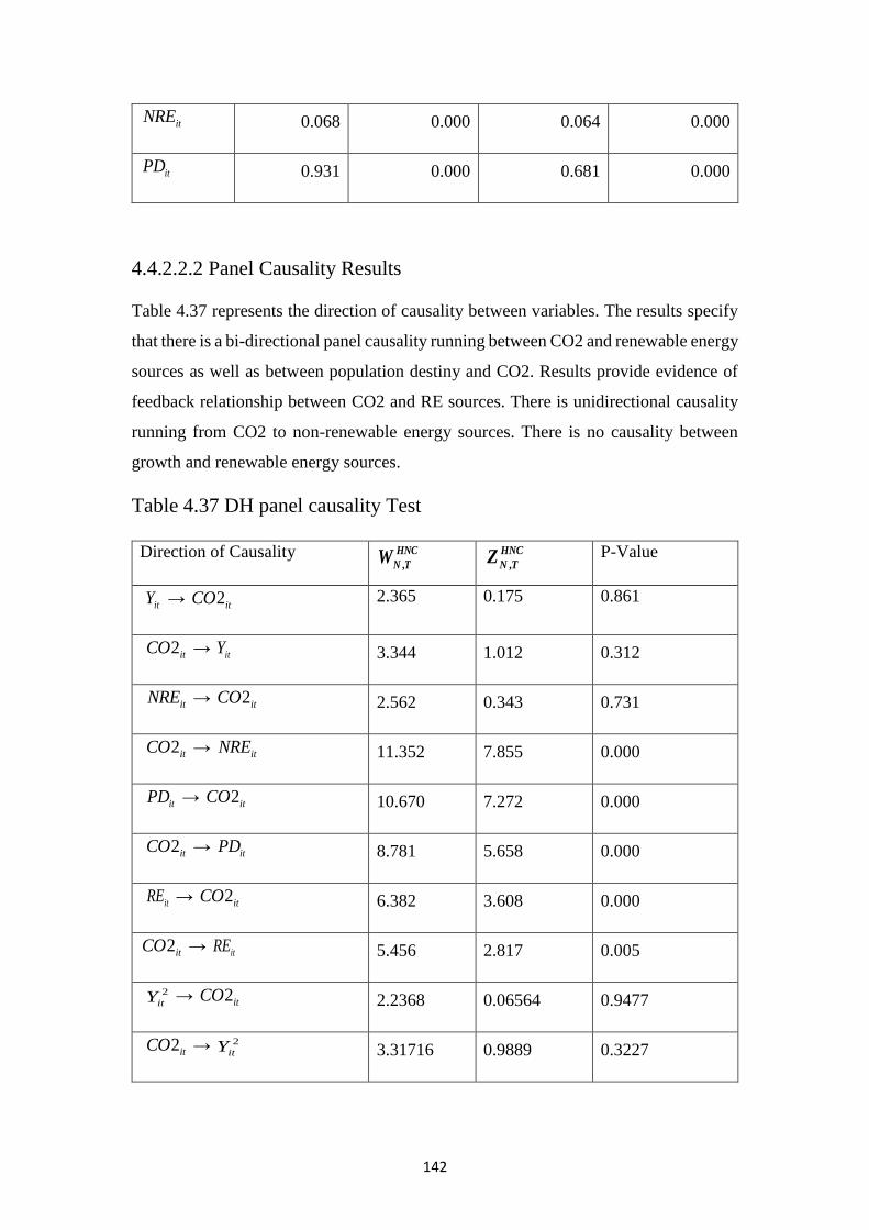
142
itNRE 0.068 0.000 0.064 0.000
itPD 0.931 0.000 0.681 0.000
4.4.2.2.2 Panel Causality Results
Table 4.37 represents the direction of causality between variables. The results specify
that there is a bi-directional panel causality running between CO2 and renewable energy
sources as well as between population destiny and CO2. Results provide evidence of
feedback relationship between CO2 and RE sources. There is unidirectional causality
running from CO2 to non-renewable energy sources. There is no causality between
growth and renewable energy sources.
Table 4.37 DH panel causality Test
Direction of Causality ,
HNC
N TW ,
HNC
N TZ P-Value
itY → 2itCO 2.365 0.175 0.861
2itCO → itY 3.344 1.012 0.312
itNRE → 2itCO 2.562 0.343 0.731
2itCO → itNRE 11.352 7.855 0.000
itPD → 2itCO 10.670 7.272 0.000
2itCO → itPD 8.781 5.658 0.000
itRE → 2itCO 6.382 3.608 0.000
2itCO → itRE 5.456 2.817 0.005
2
itY → 2itCO 2.2368 0.06564 0.9477
2itCO → 2
itY 3.31716 0.9889 0.3227
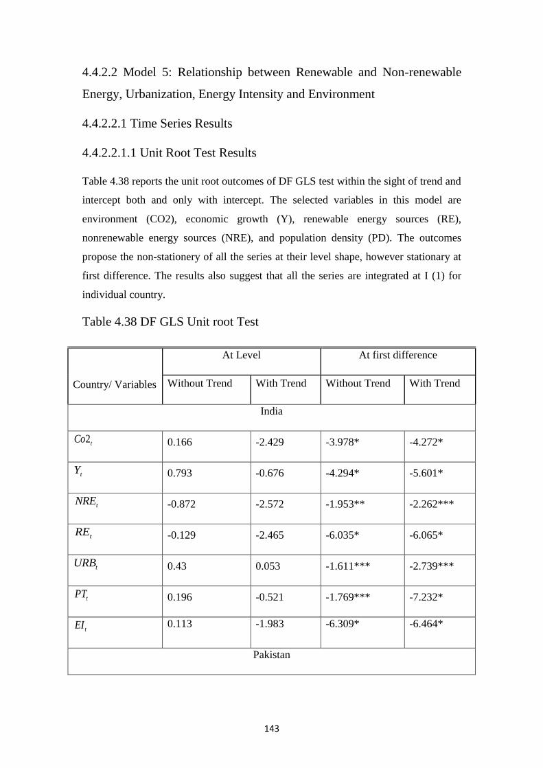
143
4.4.2.2 Model 5: Relationship between Renewable and Non-renewable
Energy, Urbanization, Energy Intensity and Environment
4.4.2.2.1 Time Series Results
4.4.2.2.1.1 Unit Root Test Results
Table 4.38 reports the unit root outcomes of DF GLS test within the sight of trend and
intercept both and only with intercept. The selected variables in this model are
environment (CO2), economic growth (Y), renewable energy sources (RE),
nonrenewable energy sources (NRE), and population density (PD). The outcomes
propose the non-stationery of all the series at their level shape, however stationary at
first difference. The results also suggest that all the series are integrated at I (1) for
individual country.
Table 4.38 DF GLS Unit root Test
Country/ Variables
At Level At first difference
Without Trend With Trend Without Trend With Trend
India
2tCo 0.166 -2.429 -3.978* -4.272*
tY 0.793 -0.676 -4.294* -5.601*
tNRE -0.872 -2.572 -1.953** -2.262***
tRE -0.129 -2.465 -6.035* -6.065*
tURB 0.43 0.053 -1.611*** -2.739***
tPT 0.196 -0.521 -1.769*** -7.232*
tEI 0.113 -1.983 -6.309* -6.464*
Pakistan
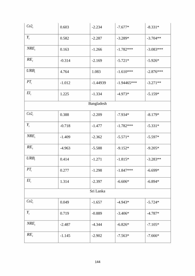
144
2tCo 0.603 -2.234 -7.677* -8.331*
tY 0.582 -2.287 -3.289* -3.704**
tNRE 0.163 -1.266 -1.782*** -3.083***
tRE -0.314 -2.169 -5.721* -5.926*
tURB 4.764 1.083 -1.610*** -2.876***
tPT -1.012 -1.44939 -1.94465*** -3.271**
tEI 1.225 -1.334 -4.973* -5.159*
Bangladesh
2tCo 0.388 -2.209 -7.934* -8.179*
tY -0.718 -1.477 -1.782*** -5.331*
tNRE -1.409 -2.362 -5.571* -5.597*
tRE -4.963 -5.588 -9.152* -9.205*
tURB 0.414 -1.271 -1.815* -3.283**
tPT 0.277 -1.298 -1.847*** -6.699*
tEI 1.314 -2.397 -6.606* -6.894*
Sri Lanka
2tCo 0.049 -1.657 -4.943* -5.724*
tY 0.719 -0.889 -3.406* -4.787*
tNRE -2.487 -4.344 -6.826* -7.105*
tRE -1.145 -2.902 -7.563* -7.666*
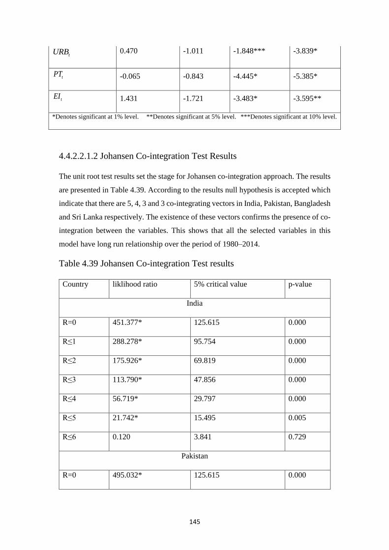
145
4.4.2.2.1.2 Johansen Co-integration Test Results
The unit root test results set the stage for Johansen co-integration approach. The results
are presented in Table 4.39. According to the results null hypothesis is accepted which
indicate that there are 5, 4, 3 and 3 co-integrating vectors in India, Pakistan, Bangladesh
and Sri Lanka respectively. The existence of these vectors confirms the presence of co-
integration between the variables. This shows that all the selected variables in this
model have long run relationship over the period of 1980–2014.
Table 4.39 Johansen Co-integration Test results
Country liklihood ratio 5% critical value p-value
India
R=0 451.377* 125.615 0.000
R≤1 288.278* 95.754 0.000
R≤2 175.926* 69.819 0.000
R≤3 113.790* 47.856 0.000
R≤4 56.719* 29.797 0.000
R≤5 21.742* 15.495 0.005
R≤6 0.120 3.841 0.729
Pakistan
R=0 495.032* 125.615 0.000
tURB 0.470 -1.011 -1.848*** -3.839*
tPT -0.065 -0.843 -4.445* -5.385*
tEI 1.431 -1.721 -3.483* -3.595**
*Denotes significant at 1% level. **Denotes significant at 5% level. ***Denotes significant at 10% level.
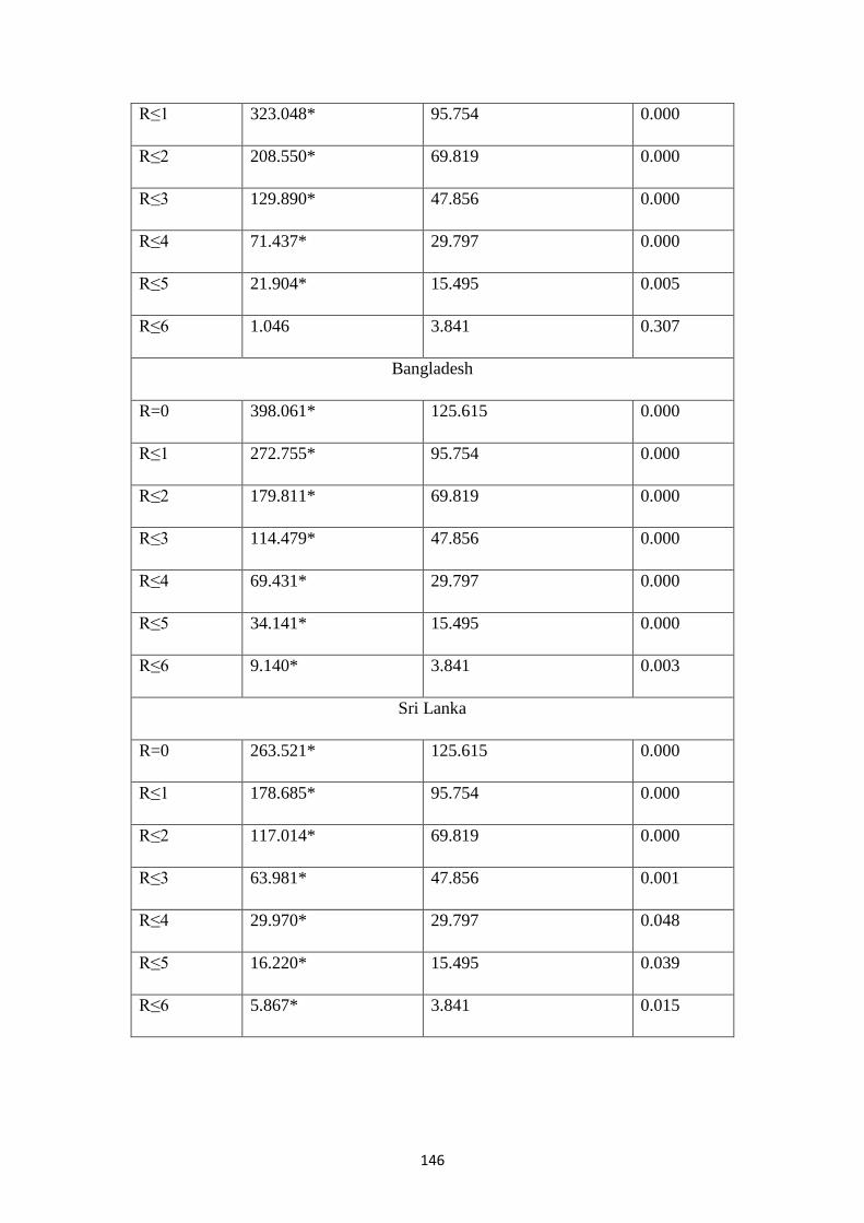
146
R≤1 323.048* 95.754 0.000
R≤2 208.550* 69.819 0.000
R≤3 129.890* 47.856 0.000
R≤4 71.437* 29.797 0.000
R≤5 21.904* 15.495 0.005
R≤6 1.046 3.841 0.307
Bangladesh
R=0 398.061* 125.615 0.000
R≤1 272.755* 95.754 0.000
R≤2 179.811* 69.819 0.000
R≤3 114.479* 47.856 0.000
R≤4 69.431* 29.797 0.000
R≤5 34.141* 15.495 0.000
R≤6 9.140* 3.841 0.003
Sri Lanka
R=0 263.521* 125.615 0.000
R≤1 178.685* 95.754 0.000
R≤2 117.014* 69.819 0.000
R≤3 63.981* 47.856 0.001
R≤4 29.970* 29.797 0.048
R≤5 16.220* 15.495 0.039
R≤6 5.867* 3.841 0.015
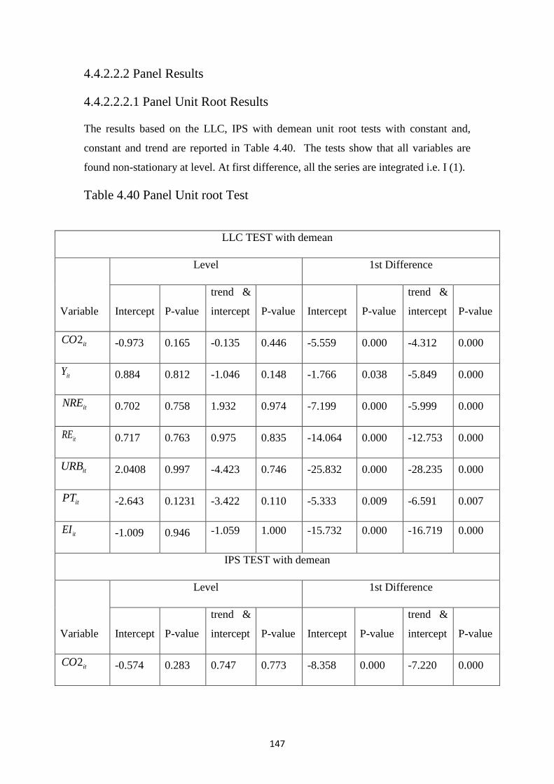
147
4.4.2.2.2 Panel Results
4.4.2.2.2.1 Panel Unit Root Results
The results based on the LLC, IPS with demean unit root tests with constant and,
constant and trend are reported in Table 4.40. The tests show that all variables are
found non-stationary at level. At first difference, all the series are integrated i.e. I (1).
Table 4.40 Panel Unit root Test
LLC TEST with demean
Variable
Level 1st Difference
Intercept P-value
trend &
intercept P-value Intercept P-value
trend &
intercept P-value
2itCO -0.973 0.165 -0.135 0.446 -5.559 0.000 -4.312 0.000
itY 0.884 0.812 -1.046 0.148 -1.766 0.038 -5.849 0.000
itNRE 0.702 0.758 1.932 0.974 -7.199 0.000 -5.999 0.000
itRE 0.717 0.763 0.975 0.835 -14.064 0.000 -12.753 0.000
itURB 2.0408 0.997 -4.423 0.746 -25.832 0.000 -28.235 0.000
itPT -2.643 0.1231 -3.422 0.110 -5.333 0.009 -6.591 0.007
itEI -1.009 0.946 -1.059 1.000 -15.732 0.000 -16.719 0.000
IPS TEST with demean
Variable
Level 1st Difference
Intercept P-value
trend &
intercept P-value Intercept P-value
trend &
intercept P-value
2itCO -0.574 0.283 0.747 0.773 -8.358 0.000 -7.220 0.000
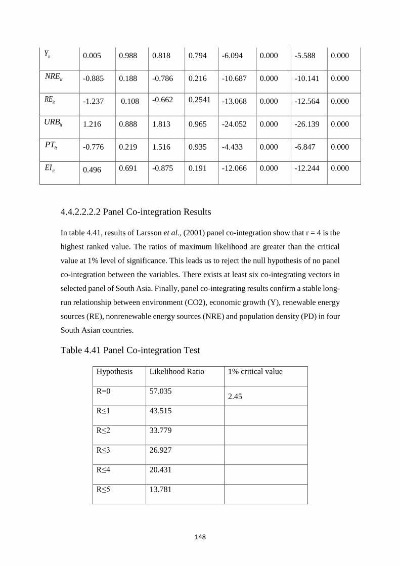
148
4.4.2.2.2.2 Panel Co-integration Results
In table 4.41, results of Larsson et al., (2001) panel co-integration show that r = 4 is the
highest ranked value. The ratios of maximum likelihood are greater than the critical
value at 1% level of significance. This leads us to reject the null hypothesis of no panel
co-integration between the variables. There exists at least six co-integrating vectors in
selected panel of South Asia. Finally, panel co-integrating results confirm a stable long-
run relationship between environment (CO2), economic growth (Y), renewable energy
sources (RE), nonrenewable energy sources (NRE) and population density (PD) in four
South Asian countries.
Table 4.41 Panel Co-integration Test
Hypothesis Likelihood Ratio 1% critical value
R=0 57.035 2.45
R≤1 43.515
R≤2 33.779
R≤3 26.927
R≤4 20.431
R≤5 13.781
itY 0.005 0.988 0.818 0.794 -6.094 0.000 -5.588 0.000
itNRE -0.885 0.188 -0.786 0.216 -10.687 0.000 -10.141 0.000
itRE -1.237 0.108 -0.662 0.2541 -13.068 0.000 -12.564 0.000
itURB 1.216 0.888 1.813 0.965 -24.052 0.000 -26.139 0.000
itPT -0.776 0.219 1.516 0.935 -4.433 0.000 -6.847 0.000
itEI 0.496 0.691 -0.875 0.191 -12.066 0.000 -12.244 0.000
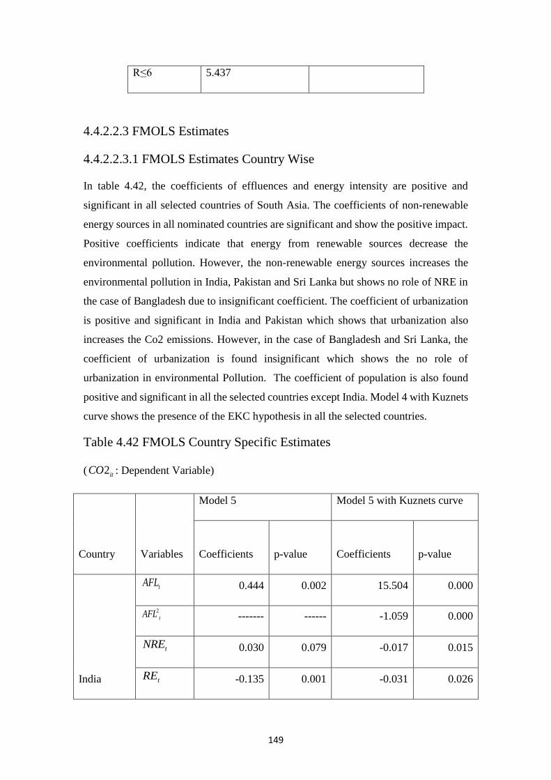
149
R≤6 5.437
4.4.2.2.3 FMOLS Estimates
4.4.2.2.3.1 FMOLS Estimates Country Wise
In table 4.42, the coefficients of effluences and energy intensity are positive and
significant in all selected countries of South Asia. The coefficients of non-renewable
energy sources in all nominated countries are significant and show the positive impact.
Positive coefficients indicate that energy from renewable sources decrease the
environmental pollution. However, the non-renewable energy sources increases the
environmental pollution in India, Pakistan and Sri Lanka but shows no role of NRE in
the case of Bangladesh due to insignificant coefficient. The coefficient of urbanization
is positive and significant in India and Pakistan which shows that urbanization also
increases the Co2 emissions. However, in the case of Bangladesh and Sri Lanka, the
coefficient of urbanization is found insignificant which shows the no role of
urbanization in environmental Pollution. The coefficient of population is also found
positive and significant in all the selected countries except India. Model 4 with Kuznets
curve shows the presence of the EKC hypothesis in all the selected countries.
Table 4.42 FMOLS Country Specific Estimates
( 2itCO : Dependent Variable)
Country
Variables
Model 5 Model 5 with Kuznets curve
Coefficients
p-value
Coefficients p-value
India
tAFL 0.444 0.002 15.504 0.000
2
tAFL ------- ------ -1.059 0.000
tNRE 0.030 0.079 -0.017 0.015
tRE -0.135 0.001 -0.031 0.026
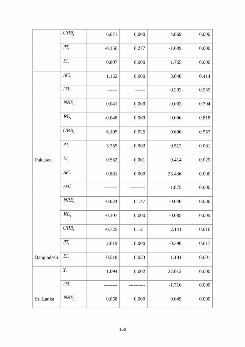
150
tURB 6.071 0.000 4.869 0.000
tPT -0.156 0.277 -1.609 0.000
tEI 0.807 0.000 1.765 0.000
Pakistan
tAFL 1.152 0.000 3.648 0.414
2
tAFL ------ ------ -0.202 0.555
tNRE 0.041 0.000 -0.002 0.794
tRE -0.048 0.069 0.006 0.818
tURB 6.105 0.025 0.696 0.553
tPT 3.355 0.003 0.512 0.081
tEI 0.532 0.001 0.414 0.029
Bangladesh
tAFL 0.881 0.000 23.436 0.000
2
tAFL -------- --------- -1.875 0.000
tNRE -0.024 0.147 -0.040 0.086
tRE -0.107 0.000 -0.085 0.009
tURB -0.725 0.121 2.141 0.016
tPT 2.619 0.000 -0.390 0.617
tEI 0.518 0.023 1.181 0.001
Sri Lanka
tY 1.094 0.002 27.012 0.000
2
tAFL -------- ---------- -1.716 0.000
tNRE 0.058 0.000 0.049 0.000
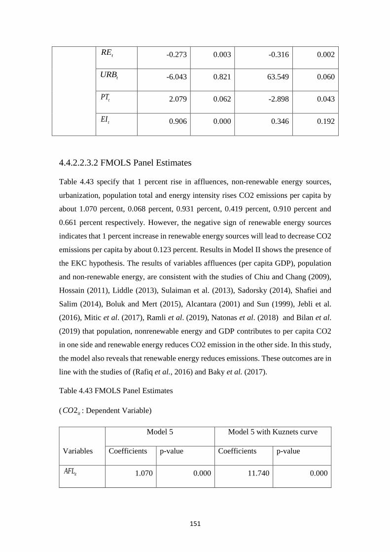
151
tRE -0.273 0.003 -0.316 0.002
tURB -6.043 0.821 63.549 0.060
tPT 2.079 0.062 -2.898 0.043
tEI 0.906 0.000 0.346 0.192
4.4.2.2.3.2 FMOLS Panel Estimates
Table 4.43 specify that 1 percent rise in affluences, non-renewable energy sources,
urbanization, population total and energy intensity rises CO2 emissions per capita by
about 1.070 percent, 0.068 percent, 0.931 percent, 0.419 percent, 0.910 percent and
0.661 percent respectively. However, the negative sign of renewable energy sources
indicates that 1 percent increase in renewable energy sources will lead to decrease CO2
emissions per capita by about 0.123 percent. Results in Model II shows the presence of
the EKC hypothesis. The results of variables affluences (per capita GDP), population
and non-renewable energy, are consistent with the studies of Chiu and Chang (2009),
Hossain (2011), Liddle (2013), Sulaiman et al. (2013), Sadorsky (2014), Shafiei and
Salim (2014), Boluk and Mert (2015), Alcantara (2001) and Sun (1999), Jebli et al.
(2016), Mitic et al. (2017), Ramli et al. (2019), Natonas et al. (2018) and Bilan et al.
(2019) that population, nonrenewable energy and GDP contributes to per capita CO2
in one side and renewable energy reduces CO2 emission in the other side. In this study,
the model also reveals that renewable energy reduces emissions. These outcomes are in
line with the studies of (Rafiq et al., 2016) and Baky et al. (2017).
Table 4.43 FMOLS Panel Estimates
( 2itCO : Dependent Variable)
Variables
Model 5 Model 5 with Kuznets curve
Coefficients p-value Coefficients p-value
itAFL 1.070 0.000 11.740 0.000
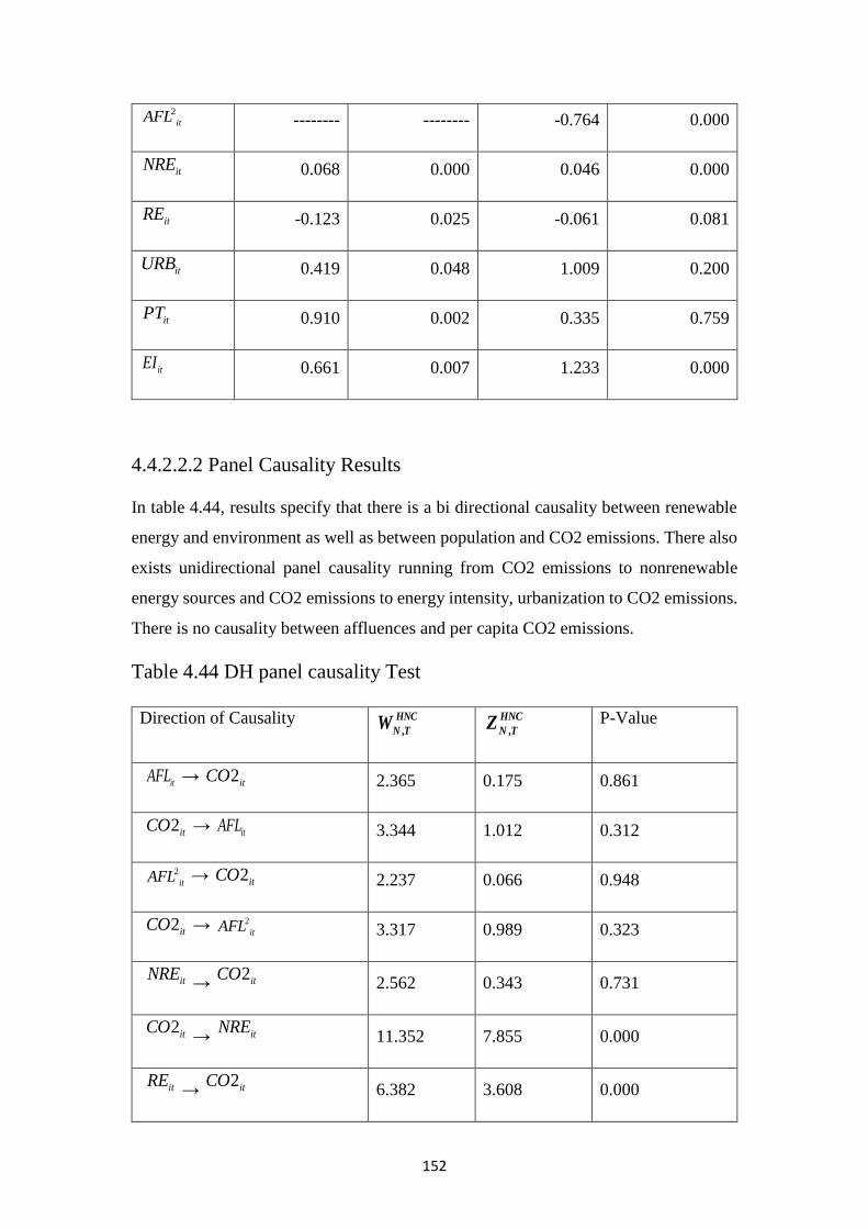
152
2
itAFL -------- -------- -0.764 0.000
itNRE 0.068 0.000 0.046 0.000
itRE -0.123 0.025 -0.061 0.081
itURB 0.419 0.048 1.009 0.200
itPT 0.910 0.002 0.335 0.759
itEI 0.661 0.007 1.233 0.000
4.4.2.2.2 Panel Causality Results
In table 4.44, results specify that there is a bi directional causality between renewable
energy and environment as well as between population and CO2 emissions. There also
exists unidirectional panel causality running from CO2 emissions to nonrenewable
energy sources and CO2 emissions to energy intensity, urbanization to CO2 emissions.
There is no causality between affluences and per capita CO2 emissions.
Table 4.44 DH panel causality Test
Direction of Causality ,
HNC
N TW ,
HNC
N TZ P-Value
itAFL → 2itCO 2.365 0.175 0.861
2itCO → itAFL 3.344 1.012 0.312
2
itAFL → 2itCO 2.237 0.066 0.948
2itCO → 2
itAFL 3.317 0.989 0.323
itNRE →
2itCO 2.562 0.343 0.731
2itCO
→ itNRE 11.352 7.855 0.000
itRE →
2itCO 6.382 3.608 0.000
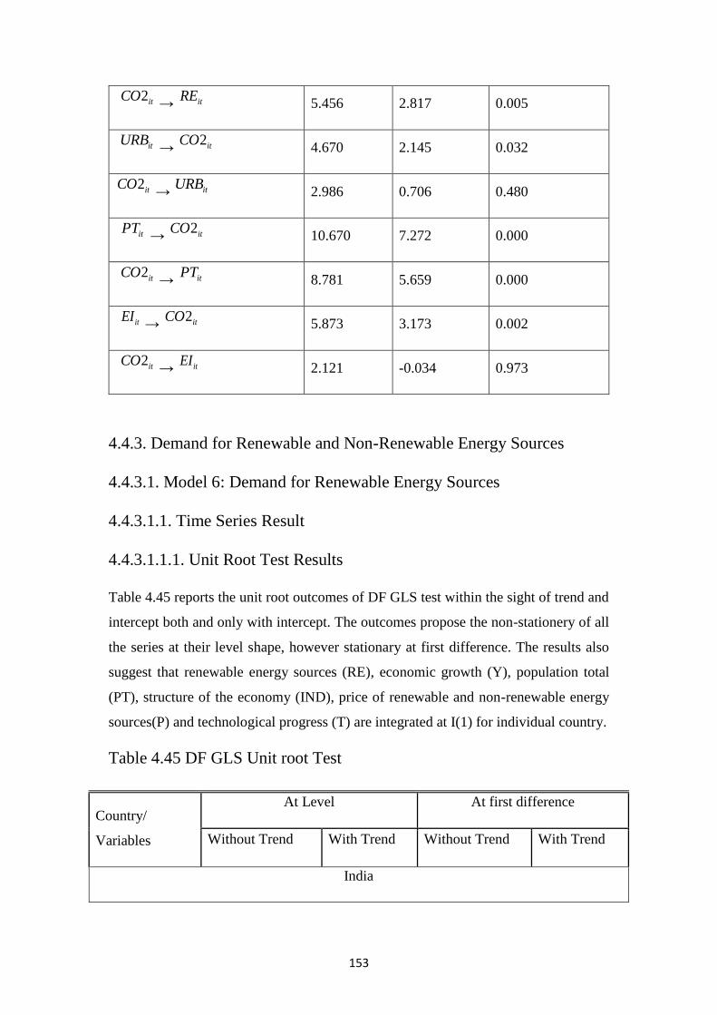
153
2itCO
→ itRE 5.456 2.817 0.005
itURB →
2itCO 4.670 2.145 0.032
2itCO → itURB
2.986 0.706 0.480
itPT →
2itCO 10.670 7.272 0.000
2itCO
→ itPT 8.781 5.659 0.000
itEI →
2itCO 5.873 3.173 0.002
2itCO
→ itEI 2.121 -0.034 0.973
4.4.3. Demand for Renewable and Non-Renewable Energy Sources
4.4.3.1. Model 6: Demand for Renewable Energy Sources
4.4.3.1.1. Time Series Result
4.4.3.1.1.1. Unit Root Test Results
Table 4.45 reports the unit root outcomes of DF GLS test within the sight of trend and
intercept both and only with intercept. The outcomes propose the non-stationery of all
the series at their level shape, however stationary at first difference. The results also
suggest that renewable energy sources (RE), economic growth (Y), population total
(PT), structure of the economy (IND), price of renewable and non-renewable energy
sources(P) and technological progress (T) are integrated at I(1) for individual country.
Table 4.45 DF GLS Unit root Test
Country/
Variables
At Level At first difference
Without Trend With Trend Without Trend With Trend
India
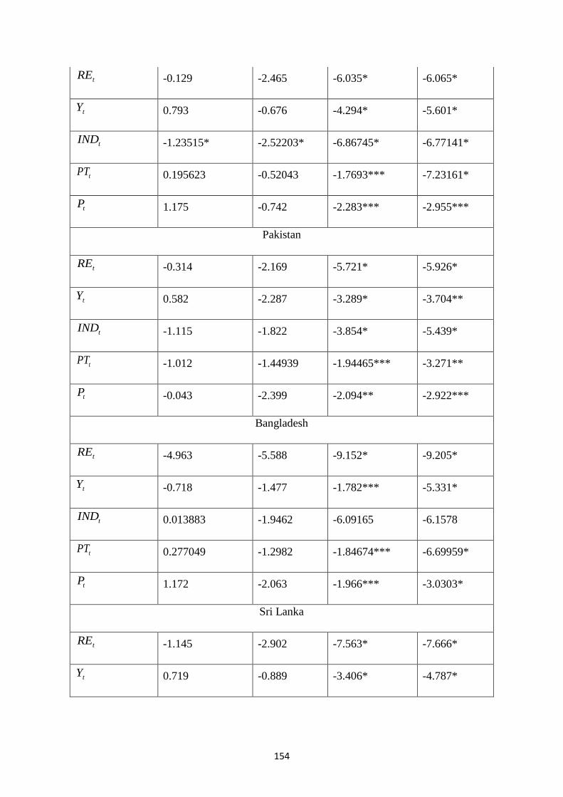
154
tRE -0.129 -2.465 -6.035* -6.065*
tY 0.793 -0.676 -4.294* -5.601*
tIND -1.23515* -2.52203* -6.86745* -6.77141*
tPT 0.195623 -0.52043 -1.7693*** -7.23161*
tP 1.175 -0.742 -2.283*** -2.955***
Pakistan
tRE -0.314 -2.169 -5.721* -5.926*
tY 0.582 -2.287 -3.289* -3.704**
tIND -1.115 -1.822 -3.854* -5.439*
tPT -1.012 -1.44939 -1.94465*** -3.271**
tP -0.043 -2.399 -2.094** -2.922***
Bangladesh
tRE -4.963 -5.588 -9.152* -9.205*
tY -0.718 -1.477 -1.782*** -5.331*
tIND 0.013883 -1.9462 -6.09165 -6.1578
tPT 0.277049 -1.2982 -1.84674*** -6.69959*
tP 1.172 -2.063 -1.966*** -3.0303*
Sri Lanka
tRE -1.145 -2.902 -7.563* -7.666*
tY 0.719 -0.889 -3.406* -4.787*
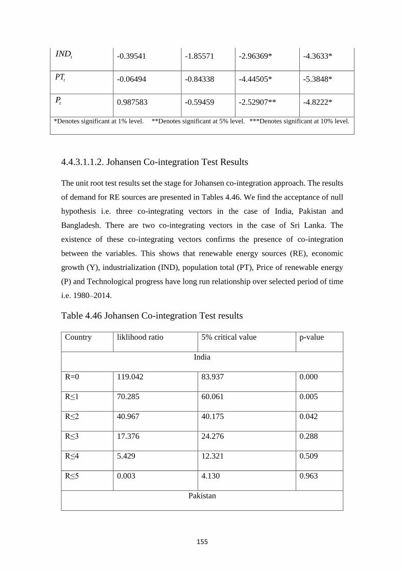
155
4.4.3.1.1.2. Johansen Co-integration Test Results
The unit root test results set the stage for Johansen co-integration approach. The results
of demand for RE sources are presented in Tables 4.46. We find the acceptance of null
hypothesis i.e. three co-integrating vectors in the case of India, Pakistan and
Bangladesh. There are two co-integrating vectors in the case of Sri Lanka. The
existence of these co-integrating vectors confirms the presence of co-integration
between the variables. This shows that renewable energy sources (RE), economic
growth (Y), industrialization (IND), population total (PT), Price of renewable energy
(P) and Technological progress have long run relationship over selected period of time
i.e. 1980–2014.
Table 4.46 Johansen Co-integration Test results
Country liklihood ratio 5% critical value p-value
India
R=0 119.042 83.937 0.000
R≤1 70.285 60.061 0.005
R≤2 40.967 40.175 0.042
R≤3 17.376 24.276 0.288
R≤4 5.429 12.321 0.509
R≤5 0.003 4.130 0.963
Pakistan
tIND -0.39541 -1.85571 -2.96369* -4.3633*
tPT -0.06494 -0.84338 -4.44505* -5.3848*
tP 0.987583 -0.59459 -2.52907** -4.8222*
*Denotes significant at 1% level. **Denotes significant at 5% level. ***Denotes significant at 10% level.
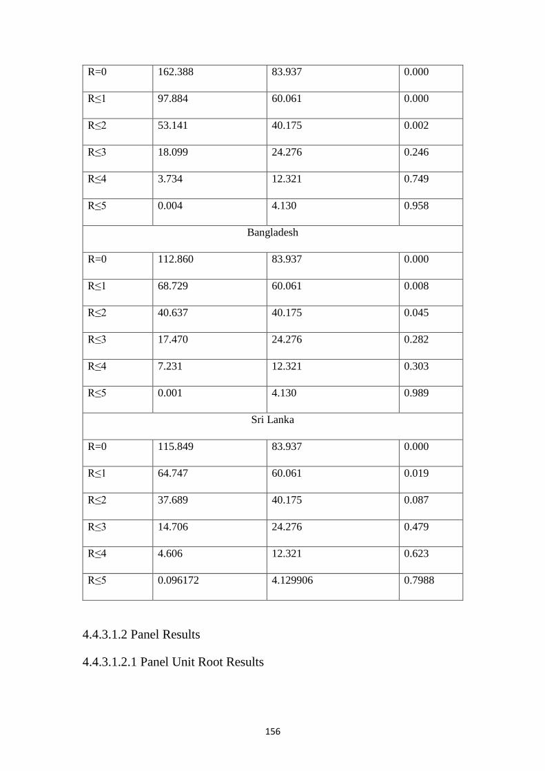
156
R=0 162.388 83.937 0.000
R≤1 97.884 60.061 0.000
R≤2 53.141 40.175 0.002
R≤3 18.099 24.276 0.246
R≤4 3.734 12.321 0.749
R≤5 0.004 4.130 0.958
Bangladesh
R=0 112.860 83.937 0.000
R≤1 68.729 60.061 0.008
R≤2 40.637 40.175 0.045
R≤3 17.470 24.276 0.282
R≤4 7.231 12.321 0.303
R≤5 0.001 4.130 0.989
Sri Lanka
R=0 115.849 83.937 0.000
R≤1 64.747 60.061 0.019
R≤2 37.689 40.175 0.087
R≤3 14.706 24.276 0.479
R≤4 4.606 12.321 0.623
R≤5 0.096172 4.129906 0.7988
4.4.3.1.2 Panel Results
4.4.3.1.2.1 Panel Unit Root Results
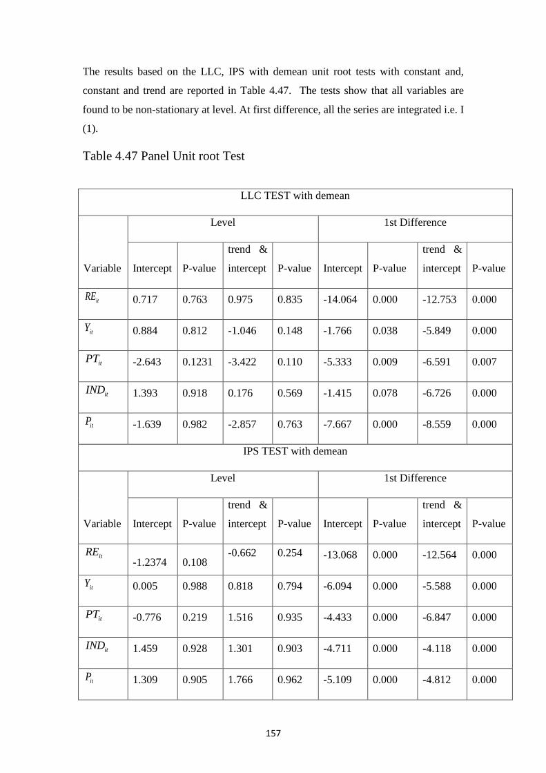
157
The results based on the LLC, IPS with demean unit root tests with constant and,
constant and trend are reported in Table 4.47. The tests show that all variables are
found to be non-stationary at level. At first difference, all the series are integrated i.e. I
(1).
Table 4.47 Panel Unit root Test
LLC TEST with demean
Variable
Level 1st Difference
Intercept P-value
trend &
intercept P-value Intercept P-value
trend &
intercept P-value
itRE 0.717 0.763 0.975 0.835 -14.064 0.000 -12.753 0.000
itY 0.884 0.812 -1.046 0.148 -1.766 0.038 -5.849 0.000
itPT -2.643 0.1231 -3.422 0.110 -5.333 0.009 -6.591 0.007
itIND 1.393 0.918 0.176 0.569 -1.415 0.078 -6.726 0.000
itP -1.639 0.982 -2.857 0.763 -7.667 0.000 -8.559 0.000
IPS TEST with demean
Variable
Level 1st Difference
Intercept P-value
trend &
intercept P-value Intercept P-value
trend &
intercept P-value
itRE
-1.2374 0.108 -0.662 0.254 -13.068 0.000 -12.564 0.000
itY 0.005 0.988 0.818 0.794 -6.094 0.000 -5.588 0.000
itPT -0.776 0.219 1.516 0.935 -4.433 0.000 -6.847 0.000
itIND 1.459 0.928 1.301 0.903 -4.711 0.000 -4.118 0.000
itP 1.309 0.905 1.766 0.962 -5.109 0.000 -4.812 0.000
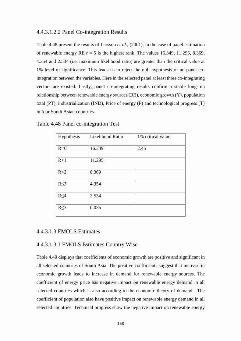
158
4.4.3.1.2.2 Panel Co-integration Results
Table 4.48 present the results of Larsson et al., (2001). In the case of panel estimation
of renewable energy RE r = 5 is the highest rank. The values 16.349, 11.295, 8.369,
4.354 and 2.534 (i.e. maximum likelihood ratio) are greater than the critical value at
1% level of significance. This leads us to reject the null hypothesis of no panel co-
integration between the variables. Here in the selected panel at least three co-integrating
vectors are existed. Lastly, panel co-integrating results confirm a stable long-run
relationship between renewable energy sources (RE), economic growth (Y), population
total (PT), industrialization (IND), Price of energy (P) and technological progress (T)
in four South Asian countries.
Table 4.48 Panel co-integration Test
Hypothesis Likelihood Ratio 1% critical value
R=0 16.349 2.45
R≤1 11.295
R≤2 8.369
R≤3 4.354
R≤4 2.534
R≤5 0.035
4.4.3.1.3 FMOLS Estimates
4.4.3.1.3.1 FMOLS Estimates Country Wise
Table 4.49 displays that coefficients of economic growth are positive and significant in
all selected countries of South Asia. The positive coefficients suggest that increase in
economic growth leads to increase in demand for renewable energy sources. The
coefficient of energy price has negative impact on renewable energy demand in all
selected countries which is also according to the economic theory of demand. The
coefficient of population also have positive impact on renewable energy demand in all
selected countries. Technical progress show the negative impact on renewable energy
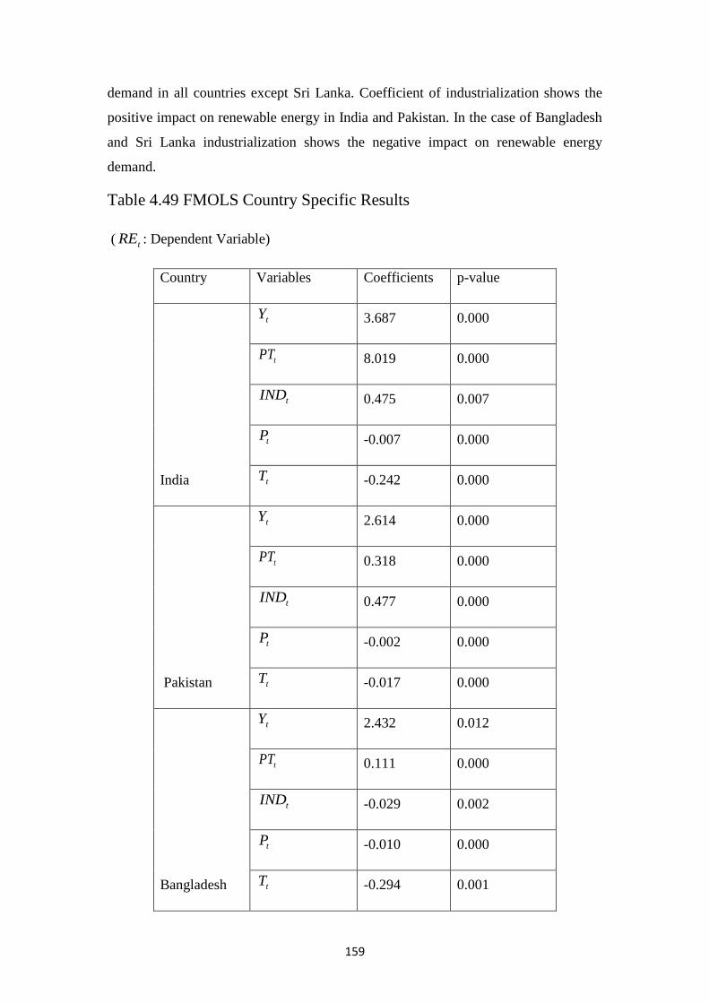
159
demand in all countries except Sri Lanka. Coefficient of industrialization shows the
positive impact on renewable energy in India and Pakistan. In the case of Bangladesh
and Sri Lanka industrialization shows the negative impact on renewable energy
demand.
Table 4.49 FMOLS Country Specific Results
( tRE : Dependent Variable)
Country Variables Coefficients p-value
India
tY 3.687 0.000
tPT 8.019 0.000
tIND 0.475 0.007
tP -0.007 0.000
tT -0.242 0.000
Pakistan
tY 2.614 0.000
tPT 0.318 0.000
tIND 0.477 0.000
tP -0.002 0.000
tT -0.017 0.000
Bangladesh
tY 2.432 0.012
tPT 0.111 0.000
tIND -0.029 0.002
tP -0.010 0.000
tT -0.294 0.001
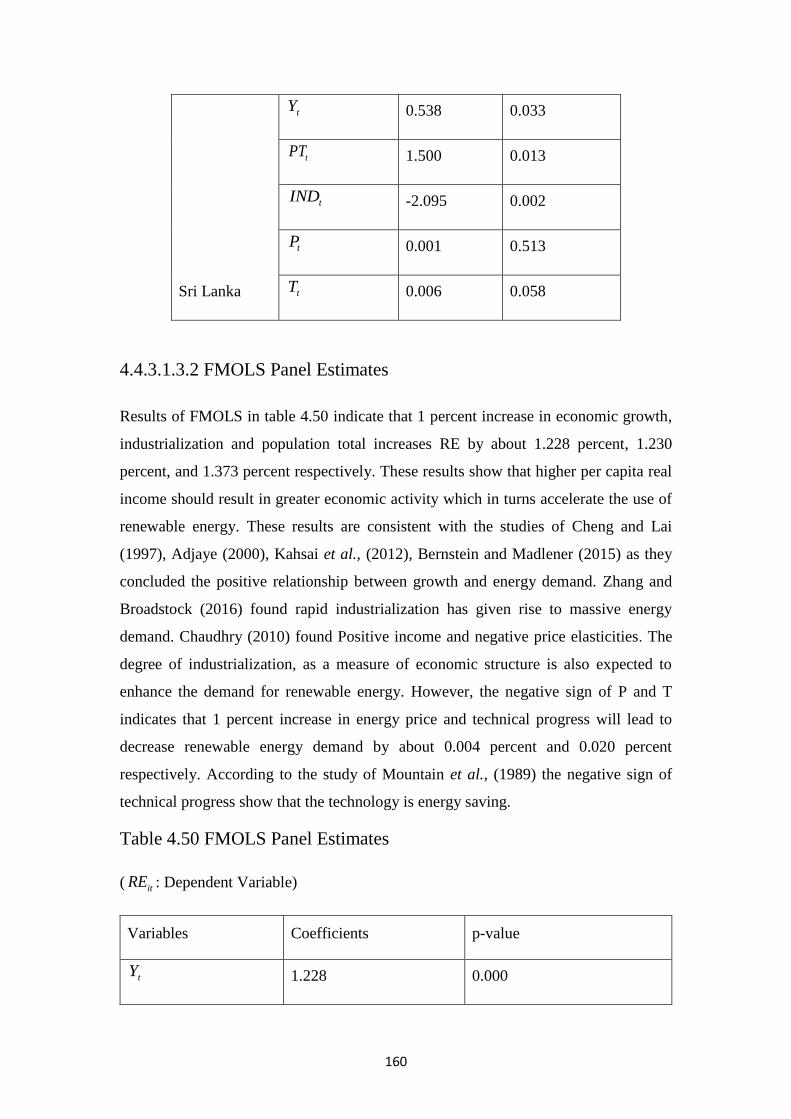
160
Sri Lanka
tY 0.538 0.033
tPT 1.500 0.013
tIND -2.095 0.002
tP 0.001 0.513
tT 0.006 0.058
4.4.3.1.3.2 FMOLS Panel Estimates
Results of FMOLS in table 4.50 indicate that 1 percent increase in economic growth,
industrialization and population total increases RE by about 1.228 percent, 1.230
percent, and 1.373 percent respectively. These results show that higher per capita real
income should result in greater economic activity which in turns accelerate the use of
renewable energy. These results are consistent with the studies of Cheng and Lai
(1997), Adjaye (2000), Kahsai et al., (2012), Bernstein and Madlener (2015) as they
concluded the positive relationship between growth and energy demand. Zhang and
Broadstock (2016) found rapid industrialization has given rise to massive energy
demand. Chaudhry (2010) found Positive income and negative price elasticities. The
degree of industrialization, as a measure of economic structure is also expected to
enhance the demand for renewable energy. However, the negative sign of P and T
indicates that 1 percent increase in energy price and technical progress will lead to
decrease renewable energy demand by about 0.004 percent and 0.020 percent
respectively. According to the study of Mountain et al., (1989) the negative sign of
technical progress show that the technology is energy saving.
Table 4.50 FMOLS Panel Estimates
( itRE : Dependent Variable)
Variables Coefficients p-value
tY 1.228 0.000
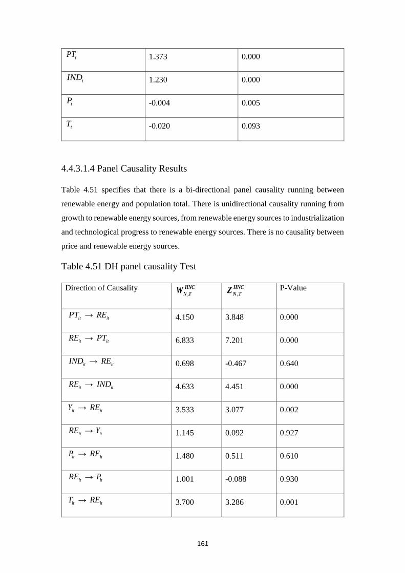
161
tPT 1.373 0.000
tIND 1.230 0.000
tP -0.004 0.005
tT -0.020 0.093
4.4.3.1.4 Panel Causality Results
Table 4.51 specifies that there is a bi-directional panel causality running between
renewable energy and population total. There is unidirectional causality running from
growth to renewable energy sources, from renewable energy sources to industrialization
and technological progress to renewable energy sources. There is no causality between
price and renewable energy sources.
Table 4.51 DH panel causality Test
Direction of Causality ,
HNC
N TW ,
HNC
N TZ P-Value
itPT → itRE 4.150 3.848 0.000
itRE → itPT 6.833 7.201 0.000
itIND → itRE 0.698 -0.467 0.640
itRE → itIND 4.633 4.451 0.000
itY → itRE 3.533 3.077 0.002
itRE → itY 1.145 0.092 0.927
itP → itRE 1.480 0.511 0.610
itRE → itP 1.001 -0.088 0.930
itT → itRE 3.700 3.286 0.001
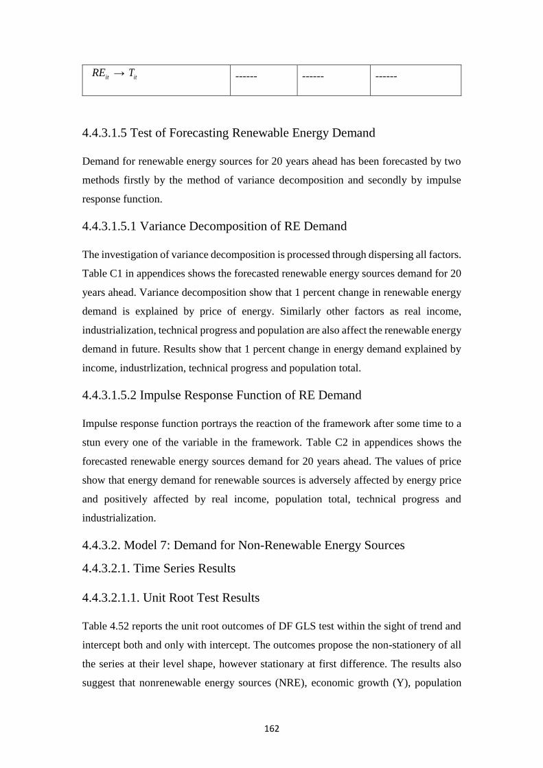
162
itRE → itT ------ ------ ------
4.4.3.1.5 Test of Forecasting Renewable Energy Demand
Demand for renewable energy sources for 20 years ahead has been forecasted by two
methods firstly by the method of variance decomposition and secondly by impulse
response function.
4.4.3.1.5.1 Variance Decomposition of RE Demand
The investigation of variance decomposition is processed through dispersing all factors.
Table C1 in appendices shows the forecasted renewable energy sources demand for 20
years ahead. Variance decomposition show that 1 percent change in renewable energy
demand is explained by price of energy. Similarly other factors as real income,
industrialization, technical progress and population are also affect the renewable energy
demand in future. Results show that 1 percent change in energy demand explained by
income, industrlization, technical progress and population total.
4.4.3.1.5.2 Impulse Response Function of RE Demand
Impulse response function portrays the reaction of the framework after some time to a
stun every one of the variable in the framework. Table C2 in appendices shows the
forecasted renewable energy sources demand for 20 years ahead. The values of price
show that energy demand for renewable sources is adversely affected by energy price
and positively affected by real income, population total, technical progress and
industrialization.
4.4.3.2. Model 7: Demand for Non-Renewable Energy Sources
4.4.3.2.1. Time Series Results
4.4.3.2.1.1. Unit Root Test Results
Table 4.52 reports the unit root outcomes of DF GLS test within the sight of trend and
intercept both and only with intercept. The outcomes propose the non-stationery of all
the series at their level shape, however stationary at first difference. The results also
suggest that nonrenewable energy sources (NRE), economic growth (Y), population
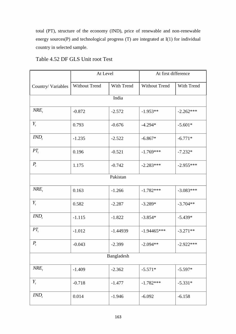
163
total (PT), structure of the economy (IND), price of renewable and non-renewable
energy sources(P) and technological progress (T) are integrated at I(1) for individual
country in selected sample.
Table 4.52 DF GLS Unit root Test
Country/ Variables
At Level At first difference
Without Trend With Trend Without Trend With Trend
India
tNRE -0.872 -2.572 -1.953** -2.262***
tY 0.793 -0.676 -4.294* -5.601*
tIND -1.235 -2.522 -6.867* -6.771*
tPT 0.196 -0.521 -1.769*** -7.232*
tP 1.175 -0.742 -2.283*** -2.955***
Pakistan
tNRE 0.163 -1.266 -1.782*** -3.083***
tY 0.582 -2.287 -3.289* -3.704**
tIND -1.115 -1.822 -3.854* -5.439*
tPT -1.012 -1.44939 -1.94465*** -3.271**
tP -0.043 -2.399 -2.094** -2.922***
Bangladesh
tNRE -1.409 -2.362 -5.571* -5.597*
tY -0.718 -1.477 -1.782*** -5.331*
tIND 0.014 -1.946 -6.092 -6.158
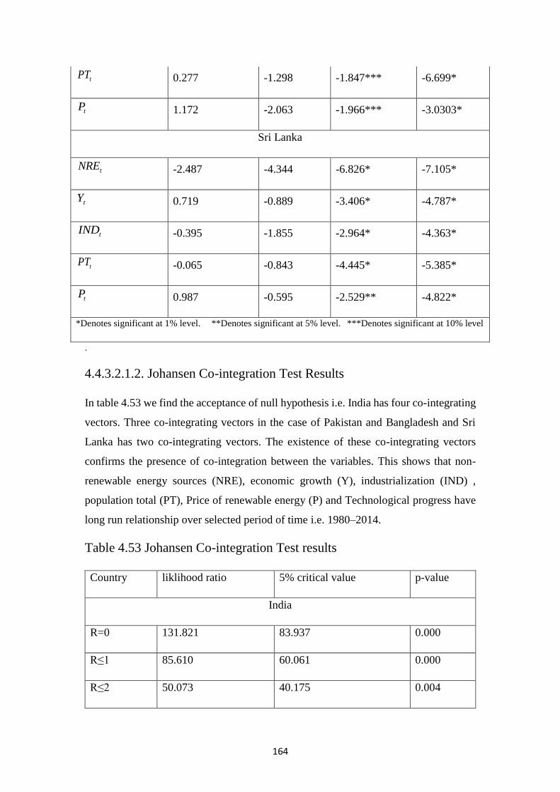
164
.
4.4.3.2.1.2. Johansen Co-integration Test Results
In table 4.53 we find the acceptance of null hypothesis i.e. India has four co-integrating
vectors. Three co-integrating vectors in the case of Pakistan and Bangladesh and Sri
Lanka has two co-integrating vectors. The existence of these co-integrating vectors
confirms the presence of co-integration between the variables. This shows that non-
renewable energy sources (NRE), economic growth (Y), industrialization (IND) ,
population total (PT), Price of renewable energy (P) and Technological progress have
long run relationship over selected period of time i.e. 1980–2014.
Table 4.53 Johansen Co-integration Test results
Country liklihood ratio 5% critical value p-value
India
R=0 131.821 83.937 0.000
R≤1 85.610 60.061 0.000
R≤2 50.073 40.175 0.004
tPT 0.277 -1.298 -1.847*** -6.699*
tP 1.172 -2.063 -1.966*** -3.0303*
Sri Lanka
tNRE -2.487 -4.344 -6.826* -7.105*
tY 0.719 -0.889 -3.406* -4.787*
tIND -0.395 -1.855 -2.964* -4.363*
tPT -0.065 -0.843 -4.445* -5.385*
tP 0.987 -0.595 -2.529** -4.822*
*Denotes significant at 1% level. **Denotes significant at 5% level. ***Denotes significant at 10% level
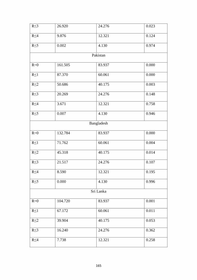
165
R≤3 26.920 24.276 0.023
R≤4 9.876 12.321 0.124
R≤5 0.002 4.130 0.974
Pakistan
R=0 161.505 83.937 0.000
R≤1 87.370 60.061 0.000
R≤2 50.686 40.175 0.003
R≤3 20.269 24.276 0.148
R≤4 3.671 12.321 0.758
R≤5 0.007 4.130 0.946
Bangladesh
R=0 132.784 83.937 0.000
R≤1 71.762 60.061 0.004
R≤2 45.318 40.175 0.014
R≤3 21.517 24.276 0.107
R≤4 8.590 12.321 0.195
R≤5 0.000 4.130 0.996
Sri Lanka
R=0 104.720 83.937 0.001
R≤1 67.172 60.061 0.011
R≤2 39.904 40.175 0.053
R≤3 16.240 24.276 0.362
R≤4 7.738 12.321 0.258
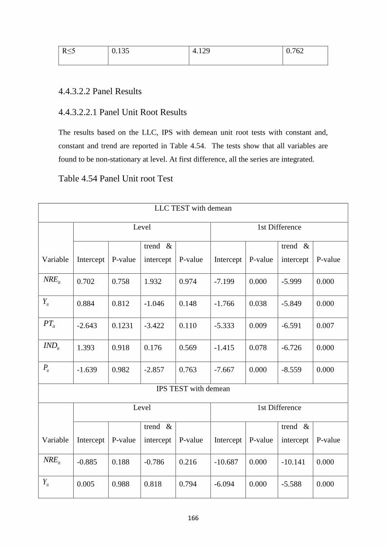
166
R≤5 0.135 4.129 0.762
4.4.3.2.2 Panel Results
4.4.3.2.2.1 Panel Unit Root Results
The results based on the LLC, IPS with demean unit root tests with constant and,
constant and trend are reported in Table 4.54. The tests show that all variables are
found to be non-stationary at level. At first difference, all the series are integrated.
Table 4.54 Panel Unit root Test
LLC TEST with demean
Variable
Level 1st Difference
Intercept P-value
trend &
intercept P-value Intercept P-value
trend &
intercept P-value
itNRE 0.702 0.758 1.932 0.974 -7.199 0.000 -5.999 0.000
itY 0.884 0.812 -1.046 0.148 -1.766 0.038 -5.849 0.000
itPT -2.643 0.1231 -3.422 0.110 -5.333 0.009 -6.591 0.007
itIND 1.393 0.918 0.176 0.569 -1.415 0.078 -6.726 0.000
itP -1.639 0.982 -2.857 0.763 -7.667 0.000 -8.559 0.000
IPS TEST with demean
Variable
Level 1st Difference
Intercept P-value
trend &
intercept P-value Intercept P-value
trend &
intercept P-value
itNRE -0.885 0.188 -0.786 0.216 -10.687 0.000 -10.141 0.000
itY 0.005 0.988 0.818 0.794 -6.094 0.000 -5.588 0.000
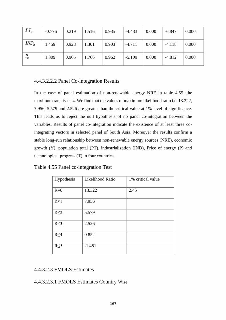
167
4.4.3.2.2.2 Panel Co-integration Results
In the case of panel estimation of non-renewable energy NRE in table 4.55, the
maximum rank is r = 4. We find that the values of maximum likelihood ratio i.e. 13.322,
7.956, 5.579 and 2.526 are greater than the critical value at 1% level of significance.
This leads us to reject the null hypothesis of no panel co-integration between the
variables. Results of panel co-integration indicate the existence of at least three co-
integrating vectors in selected panel of South Asia. Moreover the results confirm a
stable long-run relationship between non-renewable energy sources (NRE), economic
growth (Y), population total (PT), industrialization (IND), Price of energy (P) and
technological progress (T) in four countries.
Table 4.55 Panel co-integration Test
Hypothesis Likelihood Ratio 1% critical value
R=0 13.322 2.45
R≤1 7.956
R≤2 5.579
R≤3 2.526
R≤4 0.852
R≤5 -1.481
4.4.3.2.3 FMOLS Estimates
4.4.3.2.3.1 FMOLS Estimates Country Wise
itPT -0.776 0.219 1.516 0.935 -4.433 0.000 -6.847 0.000
itIND 1.459 0.928 1.301 0.903 -4.711 0.000 -4.118 0.000
itP 1.309 0.905 1.766 0.962 -5.109 0.000 -4.812 0.000
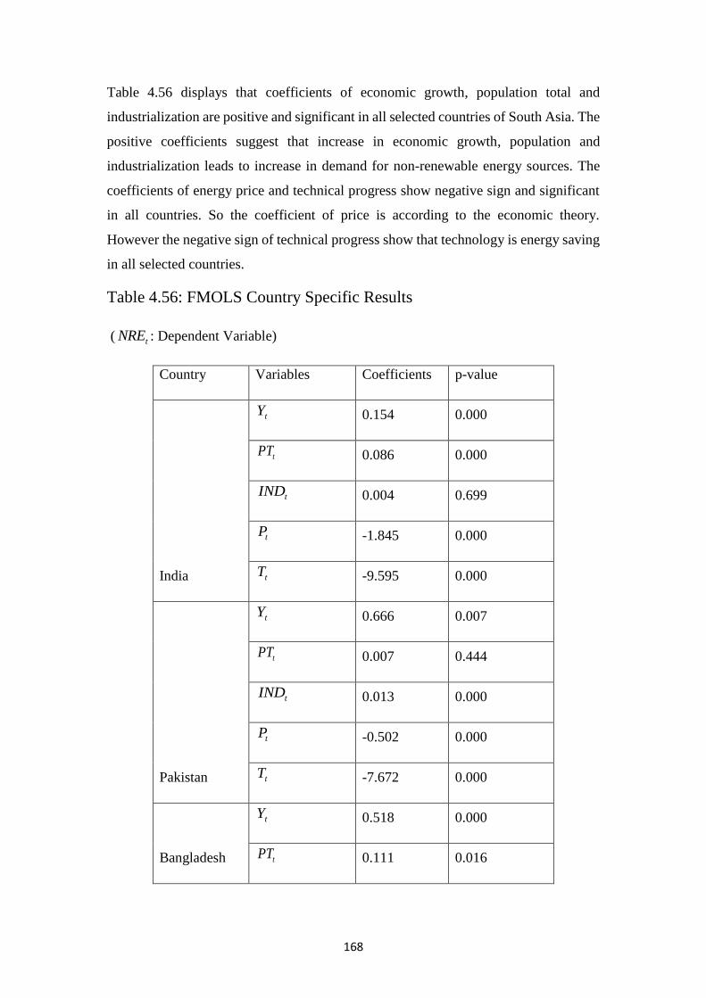
168
Table 4.56 displays that coefficients of economic growth, population total and
industrialization are positive and significant in all selected countries of South Asia. The
positive coefficients suggest that increase in economic growth, population and
industrialization leads to increase in demand for non-renewable energy sources. The
coefficients of energy price and technical progress show negative sign and significant
in all countries. So the coefficient of price is according to the economic theory.
However the negative sign of technical progress show that technology is energy saving
in all selected countries.
Table 4.56: FMOLS Country Specific Results
( tNRE : Dependent Variable)
Country Variables Coefficients p-value
India
tY 0.154 0.000
tPT 0.086 0.000
tIND 0.004 0.699
tP -1.845 0.000
tT -9.595 0.000
Pakistan
tY 0.666 0.007
tPT 0.007 0.444
tIND 0.013 0.000
tP -0.502 0.000
tT -7.672 0.000
Bangladesh
tY 0.518 0.000
tPT 0.111 0.016
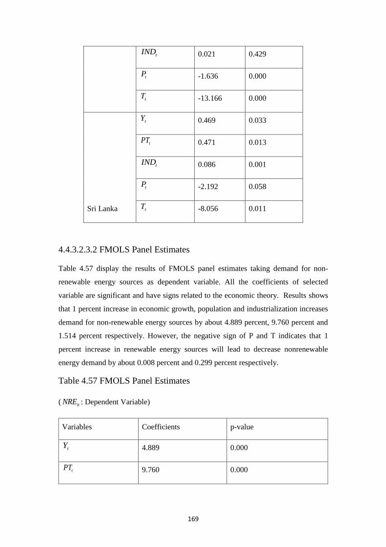
169
tIND 0.021 0.429
tP -1.636 0.000
tT -13.166 0.000
Sri Lanka
tY 0.469 0.033
tPT 0.471 0.013
tIND 0.086 0.001
tP -2.192 0.058
tT -8.056 0.011
4.4.3.2.3.2 FMOLS Panel Estimates
Table 4.57 display the results of FMOLS panel estimates taking demand for non-
renewable energy sources as dependent variable. All the coefficients of selected
variable are significant and have signs related to the economic theory. Results shows
that 1 percent increase in economic growth, population and industrialization increases
demand for non-renewable energy sources by about 4.889 percent, 9.760 percent and
1.514 percent respectively. However, the negative sign of P and T indicates that 1
percent increase in renewable energy sources will lead to decrease nonrenewable
energy demand by about 0.008 percent and 0.299 percent respectively.
Table 4.57 FMOLS Panel Estimates
( itNRE : Dependent Variable)
Variables Coefficients p-value
tY 4.889 0.000
tPT 9.760 0.000
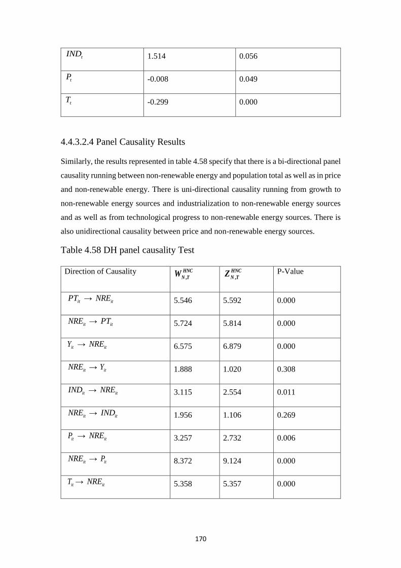
170
tIND 1.514 0.056
tP -0.008 0.049
tT -0.299 0.000
4.4.3.2.4 Panel Causality Results
Similarly, the results represented in table 4.58 specify that there is a bi-directional panel
causality running between non-renewable energy and population total as well as in price
and non-renewable energy. There is uni-directional causality running from growth to
non-renewable energy sources and industrialization to non-renewable energy sources
and as well as from technological progress to non-renewable energy sources. There is
also unidirectional causality between price and non-renewable energy sources.
Table 4.58 DH panel causality Test
Direction of Causality ,
HNC
N TW ,
HNC
N TZ P-Value
itPT → itNRE 5.546 5.592 0.000
itNRE → itPT 5.724 5.814 0.000
itY → itNRE 6.575 6.879 0.000
itNRE → itY 1.888 1.020 0.308
itIND → itNRE 3.115 2.554 0.011
itNRE → itIND 1.956 1.106 0.269
itP → itNRE 3.257 2.732 0.006
itNRE → itP 8.372 9.124 0.000
itT → itNRE 5.358 5.357 0.000
171
4.4.3.2.5 Test of Forecasting Non-Renewable Energy Demand
Demand for non-renewable energy sources for 20 years ahead has been forecasted by
two methods firstly by the method of variance decomposition and secondly by impulse
response function.
4.4.3.2.5.1 Variance Decomposition of NRE Demand
Table C3 in appendices shows the forecasted non-renewable energy sources demand
for 20 years ahead. Variance decomposition show that 1 percent change in non-
renewable energy demand is explained by price of energy. The other variable like real
income, population, technical progress and industrialization also explain the variation
in non-renewable energy demand.
4.4.3.2.5.2 Impulse Response Function of NRE Demand
Table C4 in appendices shows the forecasted non-renewable energy sources demand
for 20 years ahead. The values of price show that energy demand for non-renewable
sources is adversely affected by energy price. Similarly, it is positively affected by
population total, real income, technical progress and industrialization.
4.4.4. Impact of Renewable and Non-Renewable Energy Sources on
Energy Intensity
4.4.4.1 Model 8: Relationship between Renewable and Non-renewable
Energy, Economic Growth, Urbanization and Energy Intensity
4.4.4.1.1. Time Series Results
4.4.4.1.1.1. Unit Root Test Results
Table 4.59 reports the unit root outcomes energy intensity (EI), economic growth (Y),
renewable energy sources (RE), nonrenewable energy sources (NRE), urbanization
(URB) and population density (PD). The outcomes propose the non-stationery of all the
series at their level shape, however stationary at first difference. The results also suggest
that all variables are integrated at I(1) for individual country in selected sample.
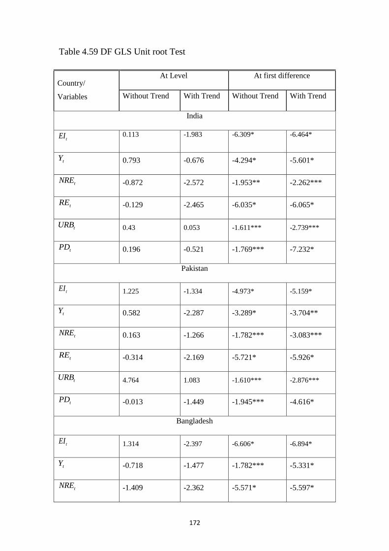
172
Table 4.59 DF GLS Unit root Test
Country/
Variables
At Level At first difference
Without Trend With Trend Without Trend With Trend
India
tEI 0.113 -1.983 -6.309* -6.464*
tY 0.793 -0.676 -4.294* -5.601*
tNRE -0.872 -2.572 -1.953** -2.262***
tRE -0.129 -2.465 -6.035* -6.065*
tURB 0.43 0.053 -1.611*** -2.739***
tPD 0.196 -0.521 -1.769*** -7.232*
Pakistan
tEI 1.225 -1.334 -4.973* -5.159*
tY 0.582 -2.287 -3.289* -3.704**
tNRE 0.163 -1.266 -1.782*** -3.083***
tRE -0.314 -2.169 -5.721* -5.926*
tURB 4.764 1.083 -1.610*** -2.876***
tPD -0.013 -1.449 -1.945*** -4.616*
Bangladesh
tEI 1.314 -2.397 -6.606* -6.894*
tY -0.718 -1.477 -1.782*** -5.331*
tNRE -1.409 -2.362 -5.571* -5.597*
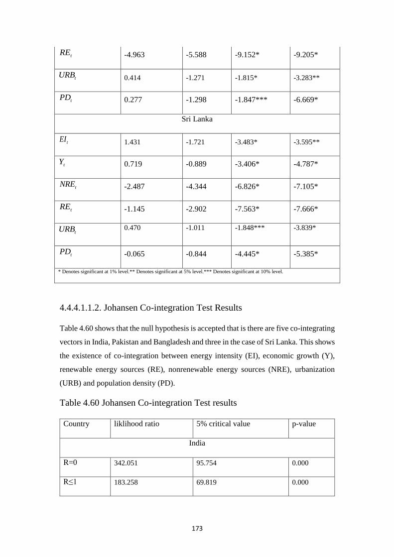
173
4.4.4.1.1.2. Johansen Co-integration Test Results
Table 4.60 shows that the null hypothesis is accepted that is there are five co-integrating
vectors in India, Pakistan and Bangladesh and three in the case of Sri Lanka. This shows
the existence of co-integration between energy intensity (EI), economic growth (Y),
renewable energy sources (RE), nonrenewable energy sources (NRE), urbanization
(URB) and population density (PD).
Table 4.60 Johansen Co-integration Test results
Country liklihood ratio 5% critical value p-value
India
R=0 342.051 95.754 0.000
R≤1 183.258 69.819 0.000
tRE -4.963 -5.588 -9.152* -9.205*
tURB 0.414 -1.271 -1.815* -3.283**
tPD 0.277 -1.298 -1.847*** -6.669*
Sri Lanka
tEI 1.431 -1.721 -3.483* -3.595**
tY 0.719 -0.889 -3.406* -4.787*
tNRE -2.487 -4.344 -6.826* -7.105*
tRE -1.145 -2.902 -7.563* -7.666*
tURB 0.470 -1.011 -1.848*** -3.839*
tPD -0.065 -0.844 -4.445* -5.385*
* Denotes significant at 1% level.** Denotes significant at 5% level.*** Denotes significant at 10% level.
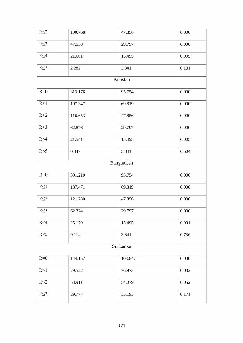
174
R≤2 100.768 47.856 0.000
R≤3 47.538 29.797 0.000
R≤4 21.601 15.495 0.005
R≤5 2.282 3.841 0.131
Pakistan
R=0 313.176 95.754 0.000
R≤1 197.347 69.819 0.000
R≤2 116.653 47.856 0.000
R≤3 62.876 29.797 0.000
R≤4 21.541 15.495 0.005
R≤5 0.447 3.841 0.504
Bangladesh
R=0 301.210 95.754 0.000
R≤1 187.471 69.819 0.000
R≤2 121.280 47.856 0.000
R≤3 62.324 29.797 0.000
R≤4 25.170 15.495 0.001
R≤5 0.114 3.841 0.736
Sri Lanka
R=0 144.152 103.847 0.000
R≤1 79.522 76.973 0.032
R≤2 53.911 54.079 0.052
R≤3 29.777 35.193 0.171
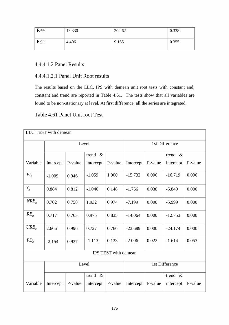
175
R≤4 13.330 20.262 0.338
R≤5 4.406 9.165 0.355
4.4.4.1.2 Panel Results
4.4.4.1.2.1 Panel Unit Root results
The results based on the LLC, IPS with demean unit root tests with constant and,
constant and trend are reported in Table 4.61. The tests show that all variables are
found to be non-stationary at level. At first difference, all the series are integrated.
Table 4.61 Panel Unit root Test
LLC TEST with demean
Variable
Level 1st Difference
Intercept P-value
trend &
intercept P-value Intercept P-value
trend &
intercept P-value
itEI -1.009 0.946 -1.059 1.000 -15.732 0.000 -16.719 0.000
itY 0.884 0.812 -1.046 0.148 -1.766 0.038 -5.849 0.000
itNRE 0.702 0.758 1.932 0.974 -7.199 0.000 -5.999 0.000
itRE 0.717 0.763 0.975 0.835 -14.064 0.000 -12.753 0.000
itURB 2.666 0.996 0.727 0.766 -23.689 0.000 -24.174 0.000
itPD -2.154 0.937 -1.113 0.133 -2.006 0.022 -1.614 0.053
IPS TEST with demean
Variable
Level 1st Difference
Intercept P-value
trend &
intercept P-value Intercept P-value
trend &
intercept P-value
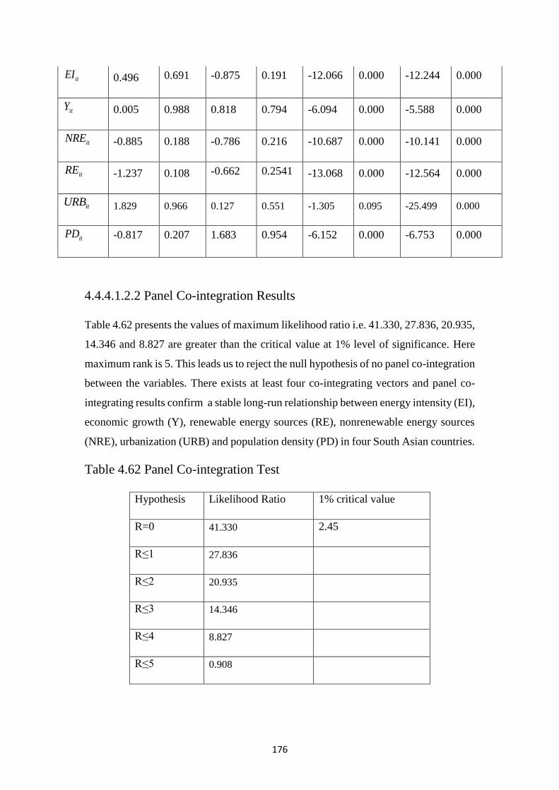
176
4.4.4.1.2.2 Panel Co-integration Results
Table 4.62 presents the values of maximum likelihood ratio i.e. 41.330, 27.836, 20.935,
14.346 and 8.827 are greater than the critical value at 1% level of significance. Here
maximum rank is 5. This leads us to reject the null hypothesis of no panel co-integration
between the variables. There exists at least four co-integrating vectors and panel co-
integrating results confirm a stable long-run relationship between energy intensity (EI),
economic growth (Y), renewable energy sources (RE), nonrenewable energy sources
(NRE), urbanization (URB) and population density (PD) in four South Asian countries.
Table 4.62 Panel Co-integration Test
Hypothesis Likelihood Ratio 1% critical value
R=0 41.330 2.45
R≤1 27.836
R≤2 20.935
R≤3 14.346
R≤4 8.827
R≤5 0.908
itEI 0.496 0.691 -0.875 0.191 -12.066 0.000 -12.244 0.000
itY 0.005 0.988 0.818 0.794 -6.094 0.000 -5.588 0.000
itNRE -0.885 0.188 -0.786 0.216 -10.687 0.000 -10.141 0.000
itRE -1.237 0.108 -0.662 0.2541 -13.068 0.000 -12.564 0.000
itURB 1.829 0.966 0.127 0.551 -1.305 0.095 -25.499 0.000
itPD -0.817 0.207 1.683 0.954 -6.152 0.000 -6.753 0.000
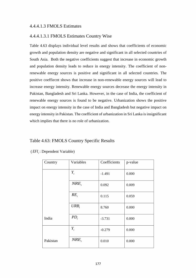
177
4.4.4.1.3 FMOLS Estimates
4.4.4.1.3.1 FMOLS Estimates Country Wise
Table 4.63 displays individual level results and shows that coefficients of economic
growth and population density are negative and significant in all selected countries of
South Asia. Both the negative coefficients suggest that increase in economic growth
and population density leads to reduce in energy intensity. The coefficient of non-
renewable energy sources is positive and significant in all selected countries. The
positive coeffiecnt shows that increase in non-renewable energy sources will lead to
increase energy intensity. Renewable energy sources decrease the energy intensity in
Pakistan, Bangladesh and Sri Lanka. However, in the case of India, the coefficient of
renewable energy sources is found to be negative. Urbanization shows the positive
impact on energy intensity in the case of India and Bangladesh but negative impact on
energy intensity in Pakistan. The coefficient of urbanization in Sri Lanka is insignificant
which implies that there is no role of urbanization.
Table 4.63: FMOLS Country Specific Results
( tEFI : Dependent Variable)
Country Variables Coefficients p-value
India
tY -1.491 0.000
tNRE 0.092 0.009
tRE 0.115 0.059
tURB 8.760 0.000
tPD -3.731 0.000
Pakistan
tY -0.279 0.000
tNRE 0.010 0.000
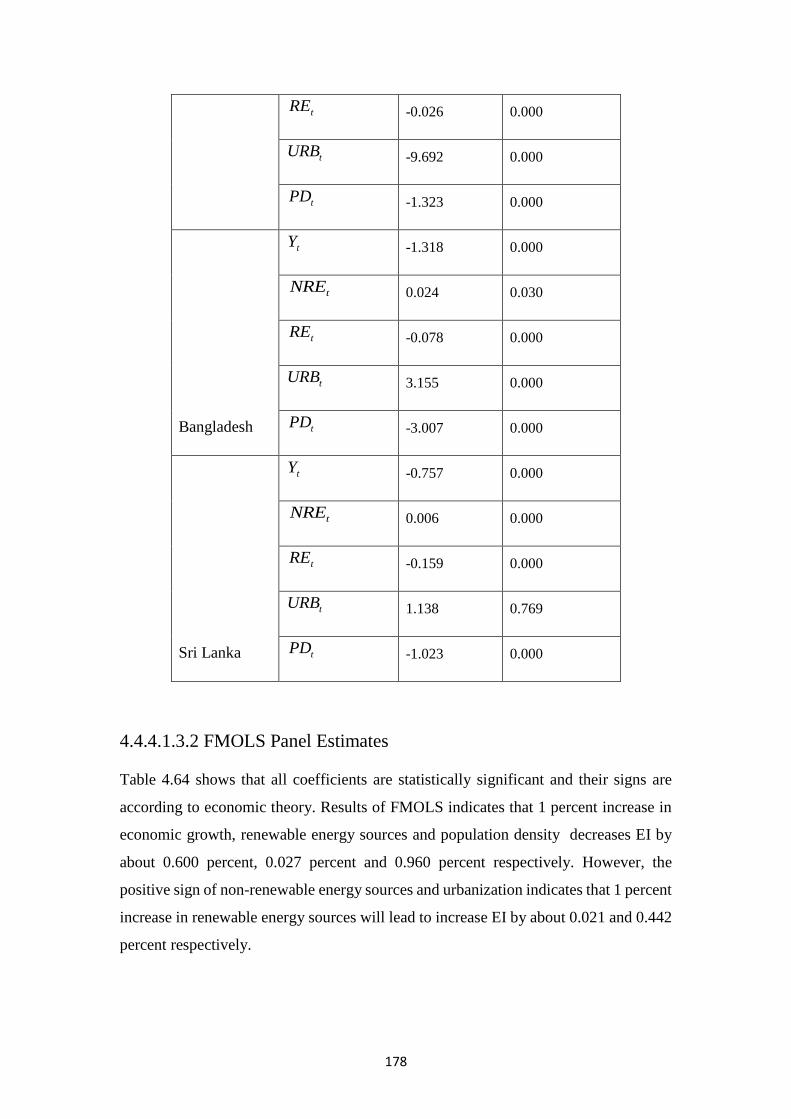
178
tRE -0.026 0.000
tURB -9.692 0.000
tPD -1.323 0.000
Bangladesh
tY -1.318 0.000
tNRE 0.024 0.030
tRE -0.078 0.000
tURB 3.155 0.000
tPD -3.007 0.000
Sri Lanka
tY -0.757 0.000
tNRE 0.006 0.000
tRE -0.159 0.000
tURB 1.138 0.769
tPD -1.023 0.000
4.4.4.1.3.2 FMOLS Panel Estimates
Table 4.64 shows that all coefficients are statistically significant and their signs are
according to economic theory. Results of FMOLS indicates that 1 percent increase in
economic growth, renewable energy sources and population density decreases EI by
about 0.600 percent, 0.027 percent and 0.960 percent respectively. However, the
positive sign of non-renewable energy sources and urbanization indicates that 1 percent
increase in renewable energy sources will lead to increase EI by about 0.021 and 0.442
percent respectively.
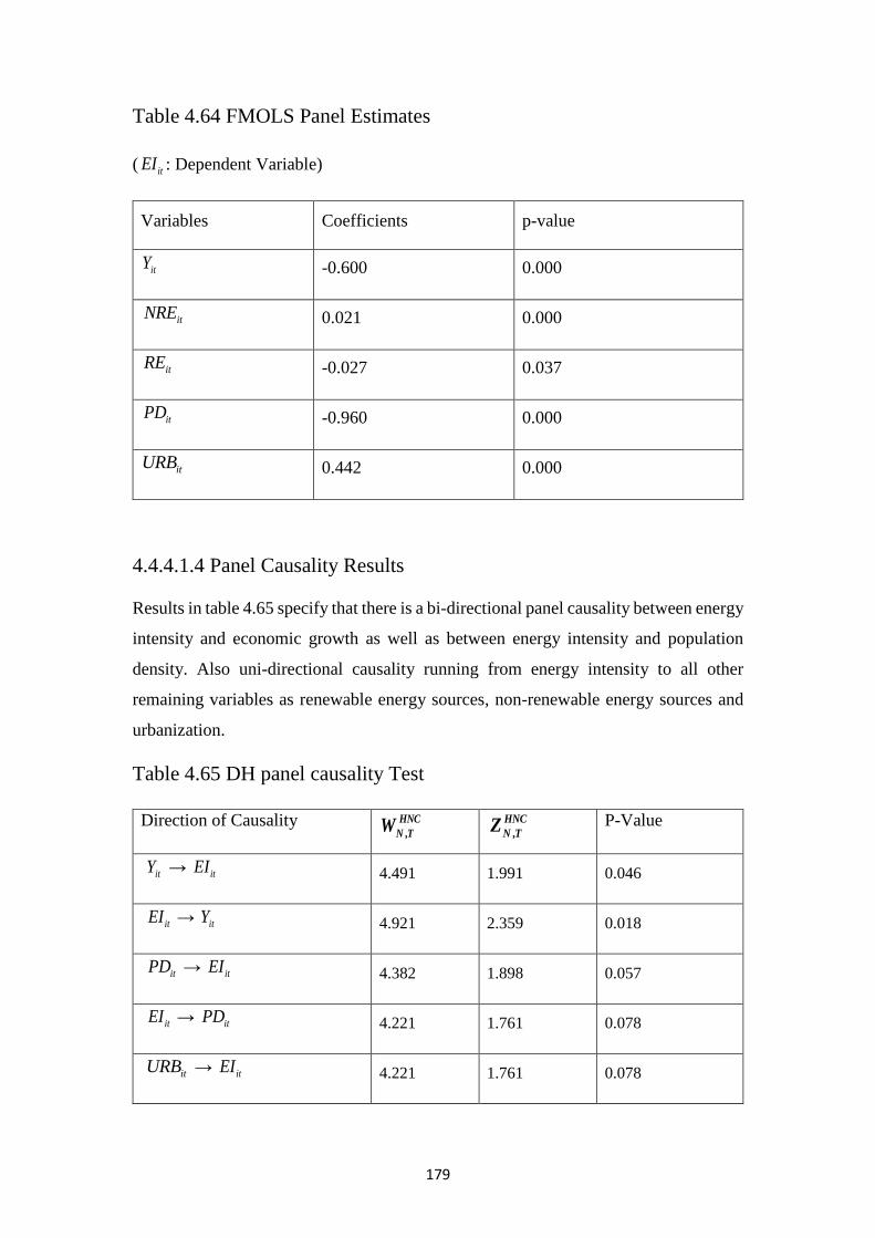
179
Table 4.64 FMOLS Panel Estimates
( itEI : Dependent Variable)
Variables Coefficients p-value
itY -0.600 0.000
itNRE 0.021 0.000
itRE -0.027 0.037
itPD -0.960 0.000
itURB 0.442 0.000
4.4.4.1.4 Panel Causality Results
Results in table 4.65 specify that there is a bi-directional panel causality between energy
intensity and economic growth as well as between energy intensity and population
density. Also uni-directional causality running from energy intensity to all other
remaining variables as renewable energy sources, non-renewable energy sources and
urbanization.
Table 4.65 DH panel causality Test
Direction of Causality ,
HNC
N TW ,
HNC
N TZ P-Value
itY → itEI 4.491 1.991 0.046
itEI → itY 4.921 2.359 0.018
itPD → itEI 4.382 1.898 0.057
itEI → itPD 4.221 1.761 0.078
itURB → itEI 4.221 1.761 0.078
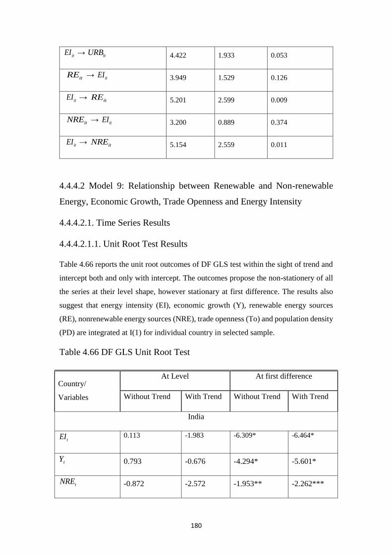
180
itEI → itURB 4.422 1.933 0.053
itRE → itEI 3.949 1.529 0.126
itEI → itRE 5.201 2.599 0.009
itNRE → itEI 3.200 0.889 0.374
itEI → itNRE 5.154 2.559 0.011
4.4.4.2 Model 9: Relationship between Renewable and Non-renewable
Energy, Economic Growth, Trade Openness and Energy Intensity
4.4.4.2.1. Time Series Results
4.4.4.2.1.1. Unit Root Test Results
Table 4.66 reports the unit root outcomes of DF GLS test within the sight of trend and
intercept both and only with intercept. The outcomes propose the non-stationery of all
the series at their level shape, however stationary at first difference. The results also
suggest that energy intensity (EI), economic growth (Y), renewable energy sources
(RE), nonrenewable energy sources (NRE), trade openness (To) and population density
(PD) are integrated at I(1) for individual country in selected sample.
Table 4.66 DF GLS Unit Root Test
Country/
Variables
At Level At first difference
Without Trend With Trend Without Trend With Trend
India
tEI 0.113 -1.983 -6.309* -6.464*
tY 0.793 -0.676 -4.294* -5.601*
tNRE -0.872 -2.572 -1.953** -2.262***
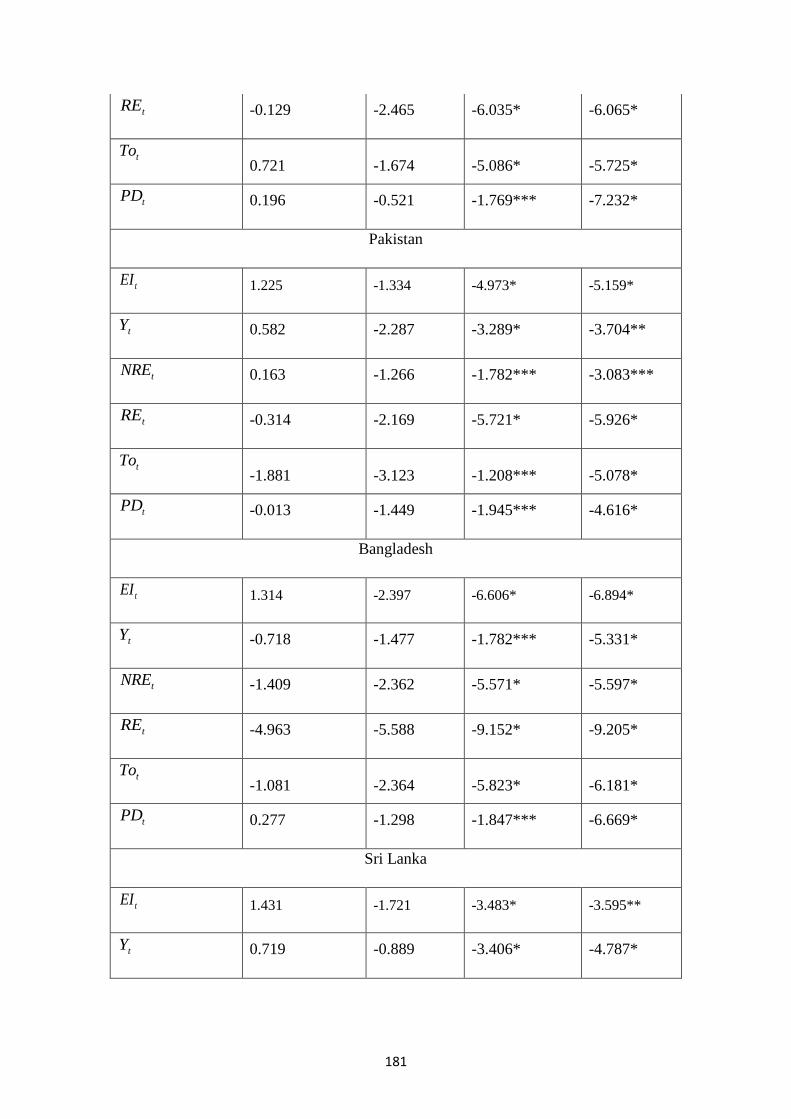
181
tRE -0.129 -2.465 -6.035* -6.065*
tTo 0.721 -1.674 -5.086* -5.725*
tPD 0.196 -0.521 -1.769*** -7.232*
Pakistan
tEI 1.225 -1.334 -4.973* -5.159*
tY 0.582 -2.287 -3.289* -3.704**
tNRE 0.163 -1.266 -1.782*** -3.083***
tRE -0.314 -2.169 -5.721* -5.926*
tTo -1.881 -3.123 -1.208*** -5.078*
tPD -0.013 -1.449 -1.945*** -4.616*
Bangladesh
tEI 1.314 -2.397 -6.606* -6.894*
tY -0.718 -1.477 -1.782*** -5.331*
tNRE -1.409 -2.362 -5.571* -5.597*
tRE -4.963 -5.588 -9.152* -9.205*
tTo -1.081 -2.364 -5.823* -6.181*
tPD 0.277 -1.298 -1.847*** -6.669*
Sri Lanka
tEI 1.431 -1.721 -3.483* -3.595**
tY 0.719 -0.889 -3.406* -4.787*
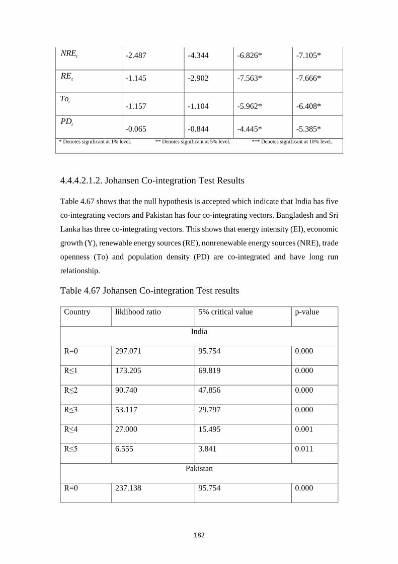
182
4.4.4.2.1.2. Johansen Co-integration Test Results
Table 4.67 shows that the null hypothesis is accepted which indicate that India has five
co-integrating vectors and Pakistan has four co-integrating vectors. Bangladesh and Sri
Lanka has three co-integrating vectors. This shows that energy intensity (EI), economic
growth (Y), renewable energy sources (RE), nonrenewable energy sources (NRE), trade
openness (To) and population density (PD) are co-integrated and have long run
relationship.
Table 4.67 Johansen Co-integration Test results
Country liklihood ratio 5% critical value p-value
India
R=0 297.071 95.754 0.000
R≤1 173.205 69.819 0.000
R≤2 90.740 47.856 0.000
R≤3 53.117 29.797 0.000
R≤4 27.000 15.495 0.001
R≤5 6.555 3.841 0.011
Pakistan
R=0 237.138 95.754 0.000
tNRE -2.487 -4.344 -6.826* -7.105*
tRE -1.145 -2.902 -7.563* -7.666*
tTo -1.157 -1.104 -5.962* -6.408*
tPD -0.065 -0.844 -4.445* -5.385*
* Denotes significant at 1% level. ** Denotes significant at 5% level. *** Denotes significant at 10% level.
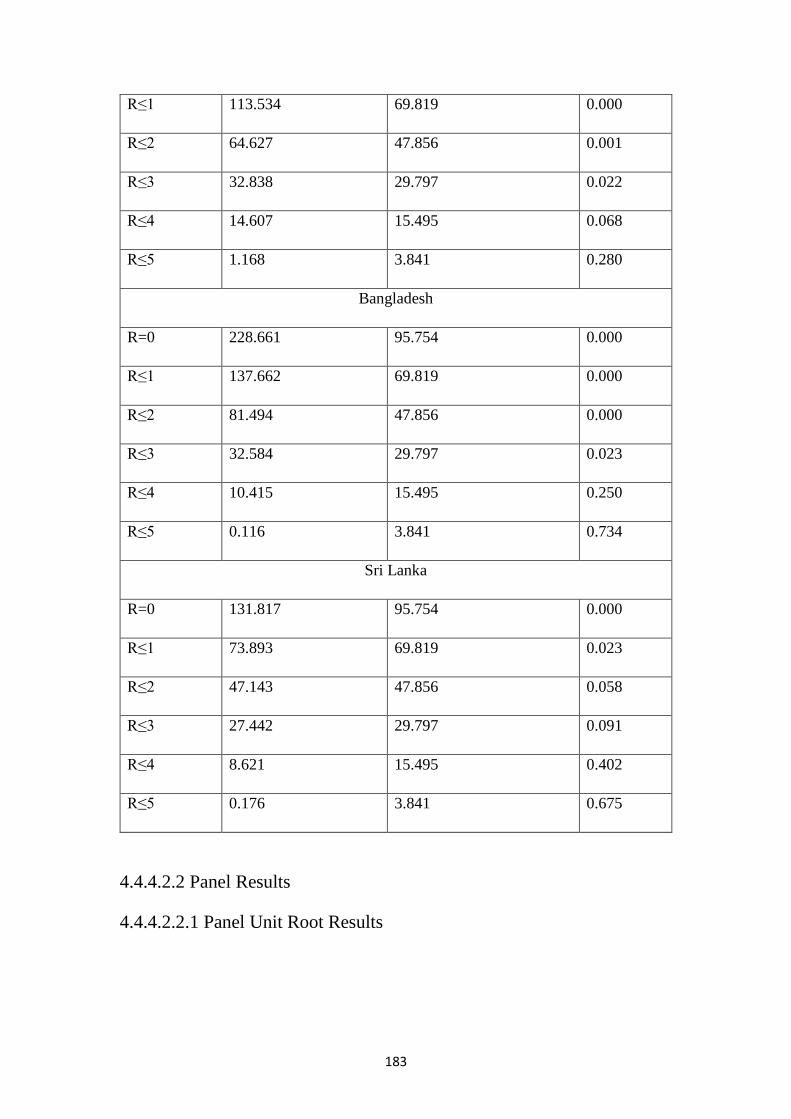
183
R≤1 113.534 69.819 0.000
R≤2 64.627 47.856 0.001
R≤3 32.838 29.797 0.022
R≤4 14.607 15.495 0.068
R≤5 1.168 3.841 0.280
Bangladesh
R=0 228.661 95.754 0.000
R≤1 137.662 69.819 0.000
R≤2 81.494 47.856 0.000
R≤3 32.584 29.797 0.023
R≤4 10.415 15.495 0.250
R≤5 0.116 3.841 0.734
Sri Lanka
R=0 131.817 95.754 0.000
R≤1 73.893 69.819 0.023
R≤2 47.143 47.856 0.058
R≤3 27.442 29.797 0.091
R≤4 8.621 15.495 0.402
R≤5 0.176 3.841 0.675
4.4.4.2.2 Panel Results
4.4.4.2.2.1 Panel Unit Root Results
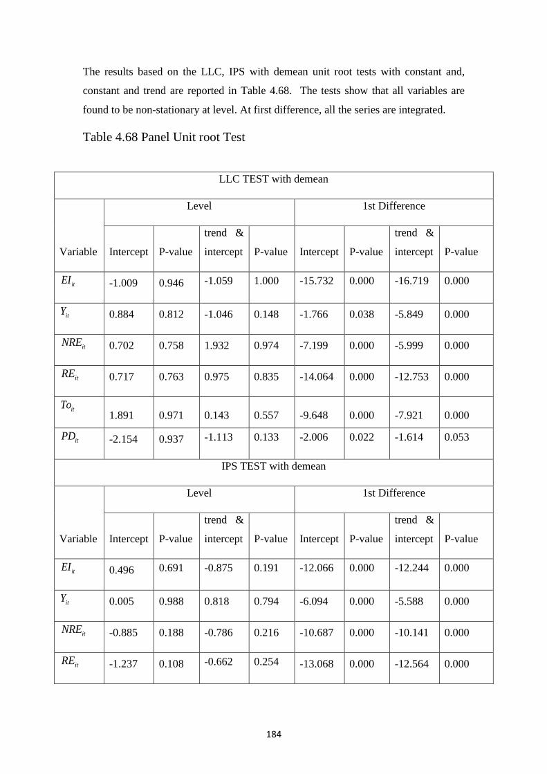
184
The results based on the LLC, IPS with demean unit root tests with constant and,
constant and trend are reported in Table 4.68. The tests show that all variables are
found to be non-stationary at level. At first difference, all the series are integrated.
Table 4.68 Panel Unit root Test
LLC TEST with demean
Variable
Level 1st Difference
Intercept P-value
trend &
intercept P-value Intercept P-value
trend &
intercept P-value
itEI -1.009 0.946 -1.059 1.000 -15.732 0.000 -16.719 0.000
itY 0.884 0.812 -1.046 0.148 -1.766 0.038 -5.849 0.000
itNRE 0.702 0.758 1.932 0.974 -7.199 0.000 -5.999 0.000
itRE 0.717 0.763 0.975 0.835 -14.064 0.000 -12.753 0.000
itTo
1.891 0.971 0.143 0.557 -9.648 0.000 -7.921 0.000
itPD -2.154 0.937 -1.113 0.133 -2.006 0.022 -1.614 0.053
IPS TEST with demean
Variable
Level 1st Difference
Intercept P-value
trend &
intercept P-value Intercept P-value
trend &
intercept P-value
itEI 0.496 0.691 -0.875 0.191 -12.066 0.000 -12.244 0.000
itY 0.005 0.988 0.818 0.794 -6.094 0.000 -5.588 0.000
itNRE -0.885 0.188 -0.786 0.216 -10.687 0.000 -10.141 0.000
itRE -1.237 0.108 -0.662 0.254 -13.068 0.000 -12.564 0.000
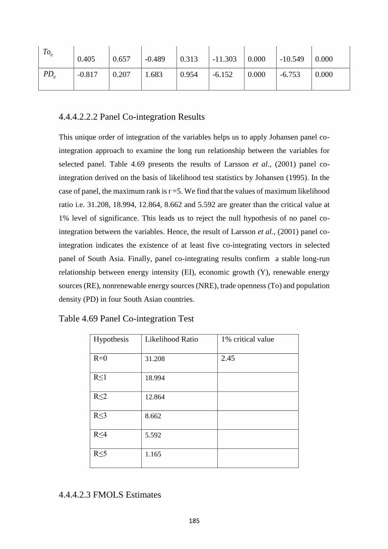
185
4.4.4.2.2.2 Panel Co-integration Results
This unique order of integration of the variables helps us to apply Johansen panel co-
integration approach to examine the long run relationship between the variables for
selected panel. Table 4.69 presents the results of Larsson et al., (2001) panel co-
integration derived on the basis of likelihood test statistics by Johansen (1995). In the
case of panel, the maximum rank is r =5. We find that the values of maximum likelihood
ratio i.e. 31.208, 18.994, 12.864, 8.662 and 5.592 are greater than the critical value at
1% level of significance. This leads us to reject the null hypothesis of no panel co-
integration between the variables. Hence, the result of Larsson et al., (2001) panel co-
integration indicates the existence of at least five co-integrating vectors in selected
panel of South Asia. Finally, panel co-integrating results confirm a stable long-run
relationship between energy intensity (EI), economic growth (Y), renewable energy
sources (RE), nonrenewable energy sources (NRE), trade openness (To) and population
density (PD) in four South Asian countries.
Table 4.69 Panel Co-integration Test
Hypothesis Likelihood Ratio 1% critical value
R=0 31.208 2.45
R≤1 18.994
R≤2 12.864
R≤3 8.662
R≤4 5.592
R≤5 1.165
4.4.4.2.3 FMOLS Estimates
itTo
0.405 0.657 -0.489 0.313 -11.303 0.000 -10.549 0.000
itPD -0.817 0.207 1.683 0.954 -6.152 0.000 -6.753 0.000
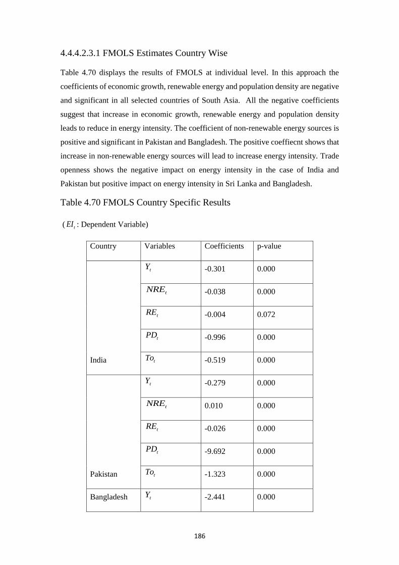
186
4.4.4.2.3.1 FMOLS Estimates Country Wise
Table 4.70 displays the results of FMOLS at individual level. In this approach the
coefficients of economic growth, renewable energy and population density are negative
and significant in all selected countries of South Asia. All the negative coefficients
suggest that increase in economic growth, renewable energy and population density
leads to reduce in energy intensity. The coefficient of non-renewable energy sources is
positive and significant in Pakistan and Bangladesh. The positive coeffiecnt shows that
increase in non-renewable energy sources will lead to increase energy intensity. Trade
openness shows the negative impact on energy intensity in the case of India and
Pakistan but positive impact on energy intensity in Sri Lanka and Bangladesh.
Table 4.70 FMOLS Country Specific Results
( tEI : Dependent Variable)
Country Variables Coefficients p-value
India
tY -0.301 0.000
tNRE -0.038 0.000
tRE -0.004 0.072
tPD -0.996 0.000
tTo -0.519 0.000
Pakistan
tY -0.279 0.000
tNRE 0.010 0.000
tRE -0.026 0.000
tPD -9.692 0.000
tTo -1.323 0.000
Bangladesh tY -2.441 0.000
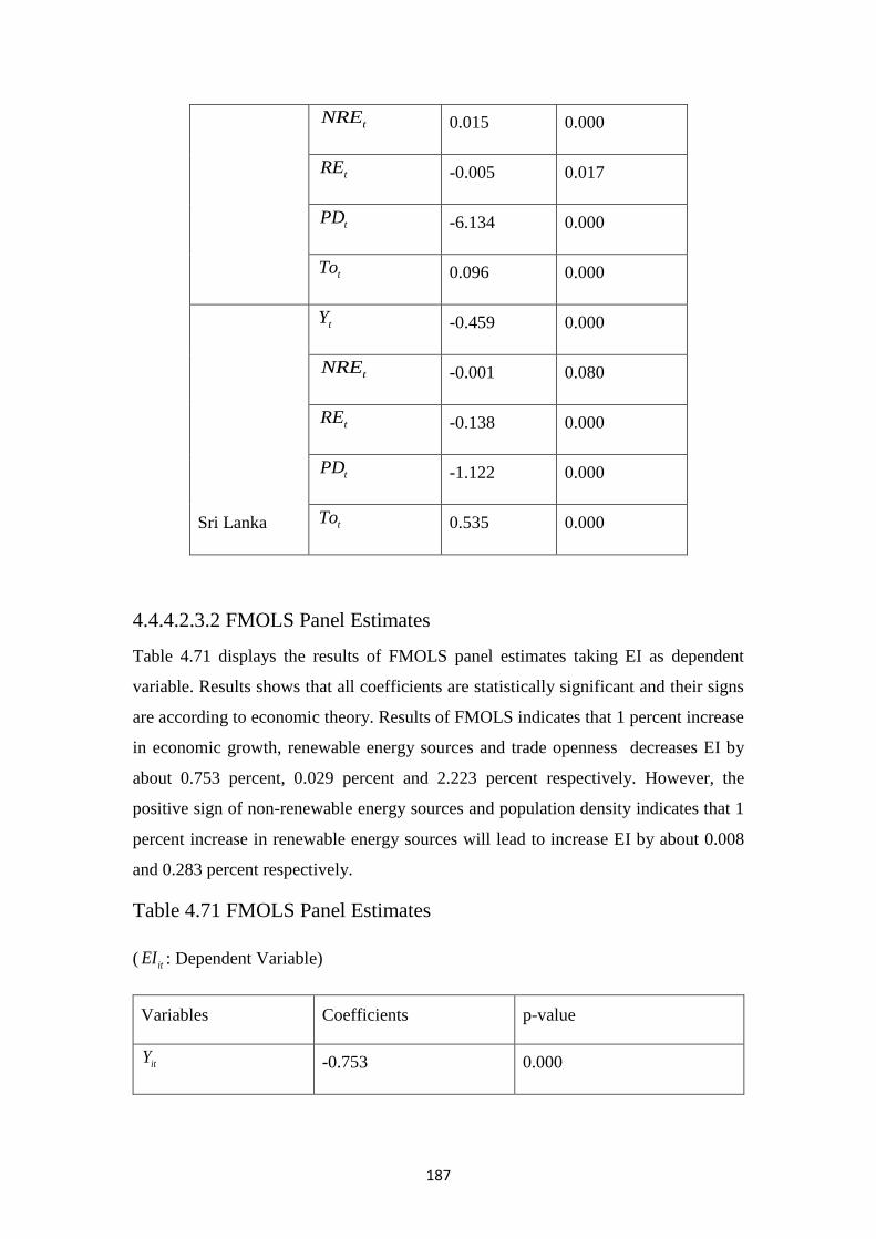
187
tNRE 0.015 0.000
tRE -0.005 0.017
tPD -6.134 0.000
tTo 0.096 0.000
Sri Lanka
tY -0.459 0.000
tNRE -0.001 0.080
tRE -0.138 0.000
tPD -1.122 0.000
tTo 0.535 0.000
4.4.4.2.3.2 FMOLS Panel Estimates
Table 4.71 displays the results of FMOLS panel estimates taking EI as dependent
variable. Results shows that all coefficients are statistically significant and their signs
are according to economic theory. Results of FMOLS indicates that 1 percent increase
in economic growth, renewable energy sources and trade openness decreases EI by
about 0.753 percent, 0.029 percent and 2.223 percent respectively. However, the
positive sign of non-renewable energy sources and population density indicates that 1
percent increase in renewable energy sources will lead to increase EI by about 0.008
and 0.283 percent respectively.
Table 4.71 FMOLS Panel Estimates
( itEI : Dependent Variable)
Variables Coefficients p-value
itY -0.753 0.000
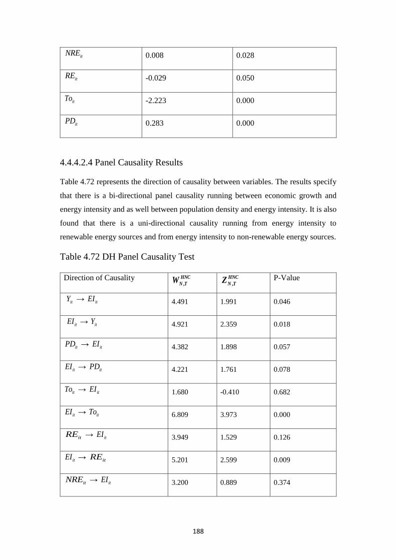
188
itNRE 0.008 0.028
itRE -0.029 0.050
itTo -2.223 0.000
itPD 0.283 0.000
4.4.4.2.4 Panel Causality Results
Table 4.72 represents the direction of causality between variables. The results specify
that there is a bi-directional panel causality running between economic growth and
energy intensity and as well between population density and energy intensity. It is also
found that there is a uni-directional causality running from energy intensity to
renewable energy sources and from energy intensity to non-renewable energy sources.
Table 4.72 DH Panel Causality Test
Direction of Causality ,
HNC
N TW ,
HNC
N TZ P-Value
itY → itEI 4.491 1.991 0.046
itEI → itY 4.921 2.359 0.018
itPD → itEI 4.382 1.898 0.057
itEI → itPD 4.221 1.761 0.078
itTo → itEI 1.680 -0.410 0.682
itEI → itTo 6.809 3.973 0.000
itRE → itEI 3.949 1.529 0.126
itEI → itRE 5.201 2.599 0.009
itNRE → itEI 3.200 0.889 0.374
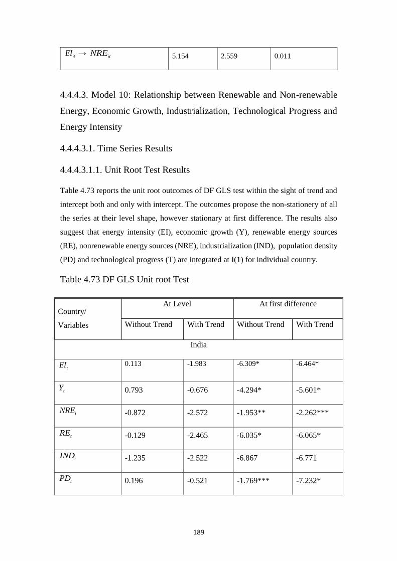
189
itEI → itNRE 5.154 2.559 0.011
4.4.4.3. Model 10: Relationship between Renewable and Non-renewable
Energy, Economic Growth, Industrialization, Technological Progress and
Energy Intensity
4.4.4.3.1. Time Series Results
4.4.4.3.1.1. Unit Root Test Results
Table 4.73 reports the unit root outcomes of DF GLS test within the sight of trend and
intercept both and only with intercept. The outcomes propose the non-stationery of all
the series at their level shape, however stationary at first difference. The results also
suggest that energy intensity (EI), economic growth (Y), renewable energy sources
(RE), nonrenewable energy sources (NRE), industrialization (IND), population density
(PD) and technological progress (T) are integrated at I(1) for individual country.
Table 4.73 DF GLS Unit root Test
Country/
Variables
At Level At first difference
Without Trend With Trend Without Trend With Trend
India
tEI 0.113 -1.983 -6.309* -6.464*
tY 0.793 -0.676 -4.294* -5.601*
tNRE -0.872 -2.572 -1.953** -2.262***
tRE -0.129 -2.465 -6.035* -6.065*
tIND -1.235 -2.522 -6.867 -6.771
tPD 0.196 -0.521 -1.769*** -7.232*
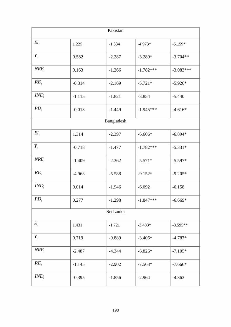
190
Pakistan
tEI 1.225 -1.334 -4.973* -5.159*
tY 0.582 -2.287 -3.289* -3.704**
tNRE 0.163 -1.266 -1.782*** -3.083***
tRE -0.314 -2.169 -5.721* -5.926*
tIND -1.115 -1.821 -3.854 -5.440
tPD -0.013 -1.449 -1.945*** -4.616*
Bangladesh
tEI 1.314 -2.397 -6.606* -6.894*
tY -0.718 -1.477 -1.782*** -5.331*
tNRE -1.409 -2.362 -5.571* -5.597*
tRE -4.963 -5.588 -9.152* -9.205*
tIND 0.014 -1.946 -6.092 -6.158
tPD 0.277 -1.298 -1.847*** -6.669*
Sri Lanka
tEI 1.431 -1.721 -3.483* -3.595**
tY 0.719 -0.889 -3.406* -4.787*
tNRE -2.487 -4.344 -6.826* -7.105*
tRE -1.145 -2.902 -7.563* -7.666*
tIND -0.395 -1.856 -2.964 -4.363
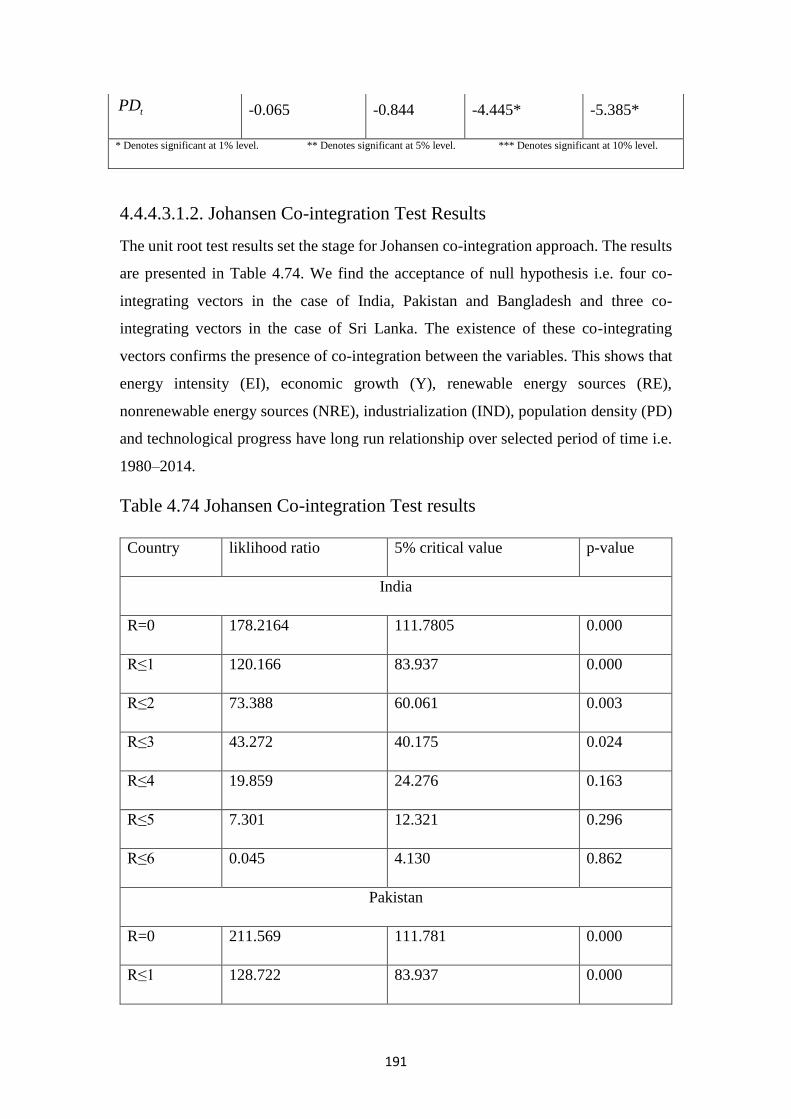
191
4.4.4.3.1.2. Johansen Co-integration Test Results
The unit root test results set the stage for Johansen co-integration approach. The results
are presented in Table 4.74. We find the acceptance of null hypothesis i.e. four co-
integrating vectors in the case of India, Pakistan and Bangladesh and three co-
integrating vectors in the case of Sri Lanka. The existence of these co-integrating
vectors confirms the presence of co-integration between the variables. This shows that
energy intensity (EI), economic growth (Y), renewable energy sources (RE),
nonrenewable energy sources (NRE), industrialization (IND), population density (PD)
and technological progress have long run relationship over selected period of time i.e.
1980–2014.
Table 4.74 Johansen Co-integration Test results
Country liklihood ratio 5% critical value p-value
India
R=0 178.2164 111.7805 0.000
R≤1 120.166 83.937 0.000
R≤2 73.388 60.061 0.003
R≤3 43.272 40.175 0.024
R≤4 19.859 24.276 0.163
R≤5 7.301 12.321 0.296
R≤6 0.045 4.130 0.862
Pakistan
R=0 211.569 111.781 0.000
R≤1 128.722 83.937 0.000
tPD -0.065 -0.844 -4.445* -5.385*
* Denotes significant at 1% level. ** Denotes significant at 5% level. *** Denotes significant at 10% level.
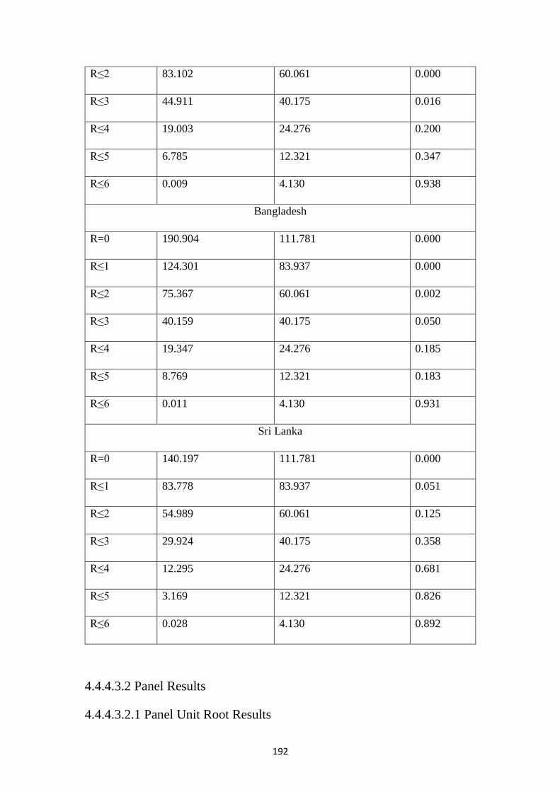
192
R≤2 83.102 60.061 0.000
R≤3 44.911 40.175 0.016
R≤4 19.003 24.276 0.200
R≤5 6.785 12.321 0.347
R≤6 0.009 4.130 0.938
Bangladesh
R=0 190.904 111.781 0.000
R≤1 124.301 83.937 0.000
R≤2 75.367 60.061 0.002
R≤3 40.159 40.175 0.050
R≤4 19.347 24.276 0.185
R≤5 8.769 12.321 0.183
R≤6 0.011 4.130 0.931
Sri Lanka
R=0 140.197 111.781 0.000
R≤1 83.778 83.937 0.051
R≤2 54.989 60.061 0.125
R≤3 29.924 40.175 0.358
R≤4 12.295 24.276 0.681
R≤5 3.169 12.321 0.826
R≤6 0.028 4.130 0.892
4.4.4.3.2 Panel Results
4.4.4.3.2.1 Panel Unit Root Results
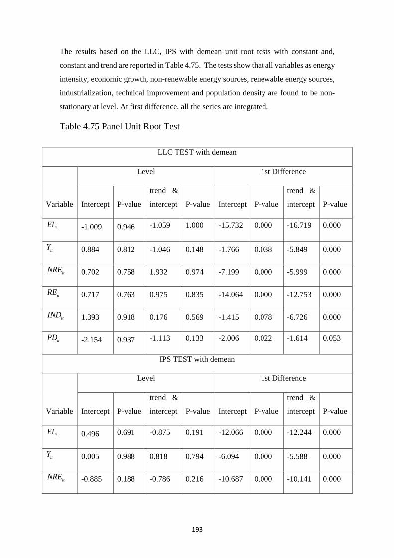
193
The results based on the LLC, IPS with demean unit root tests with constant and,
constant and trend are reported in Table 4.75. The tests show that all variables as energy
intensity, economic growth, non-renewable energy sources, renewable energy sources,
industrialization, technical improvement and population density are found to be non-
stationary at level. At first difference, all the series are integrated.
Table 4.75 Panel Unit Root Test
LLC TEST with demean
Variable
Level 1st Difference
Intercept P-value
trend &
intercept P-value Intercept P-value
trend &
intercept P-value
itEI -1.009 0.946 -1.059 1.000 -15.732 0.000 -16.719 0.000
itY 0.884 0.812 -1.046 0.148 -1.766 0.038 -5.849 0.000
itNRE 0.702 0.758 1.932 0.974 -7.199 0.000 -5.999 0.000
itRE 0.717 0.763 0.975 0.835 -14.064 0.000 -12.753 0.000
itIND 1.393 0.918 0.176 0.569 -1.415 0.078 -6.726 0.000
itPD -2.154 0.937 -1.113 0.133 -2.006 0.022 -1.614 0.053
IPS TEST with demean
Variable
Level 1st Difference
Intercept P-value
trend &
intercept P-value Intercept P-value
trend &
intercept P-value
itEI 0.496 0.691 -0.875 0.191 -12.066 0.000 -12.244 0.000
itY 0.005 0.988 0.818 0.794 -6.094 0.000 -5.588 0.000
itNRE -0.885 0.188 -0.786 0.216 -10.687 0.000 -10.141 0.000
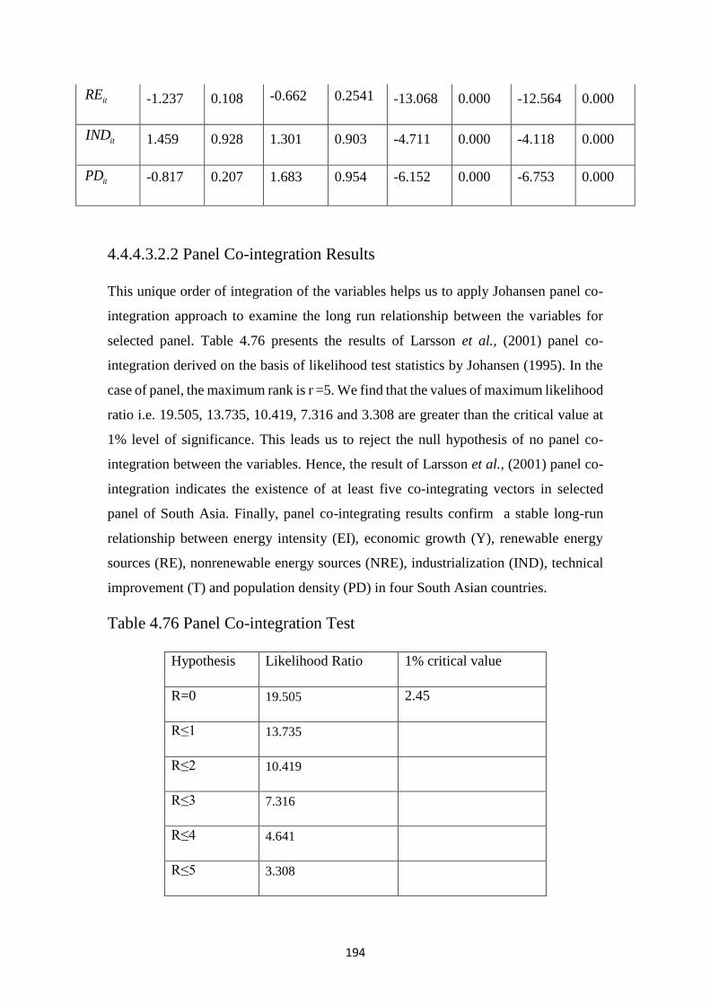
194
4.4.4.3.2.2 Panel Co-integration Results
This unique order of integration of the variables helps us to apply Johansen panel co-
integration approach to examine the long run relationship between the variables for
selected panel. Table 4.76 presents the results of Larsson et al., (2001) panel co-
integration derived on the basis of likelihood test statistics by Johansen (1995). In the
case of panel, the maximum rank is r =5. We find that the values of maximum likelihood
ratio i.e. 19.505, 13.735, 10.419, 7.316 and 3.308 are greater than the critical value at
1% level of significance. This leads us to reject the null hypothesis of no panel co-
integration between the variables. Hence, the result of Larsson et al., (2001) panel co-
integration indicates the existence of at least five co-integrating vectors in selected
panel of South Asia. Finally, panel co-integrating results confirm a stable long-run
relationship between energy intensity (EI), economic growth (Y), renewable energy
sources (RE), nonrenewable energy sources (NRE), industrialization (IND), technical
improvement (T) and population density (PD) in four South Asian countries.
Table 4.76 Panel Co-integration Test
Hypothesis Likelihood Ratio 1% critical value
R=0 19.505 2.45
R≤1 13.735
R≤2 10.419
R≤3 7.316
R≤4 4.641
R≤5 3.308
itRE -1.237 0.108 -0.662 0.2541 -13.068 0.000 -12.564 0.000
itIND 1.459 0.928 1.301 0.903 -4.711 0.000 -4.118 0.000
itPD -0.817 0.207 1.683 0.954 -6.152 0.000 -6.753 0.000
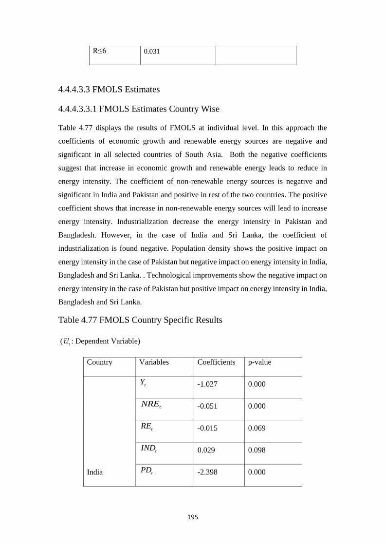
195
R≤6 0.031
4.4.4.3.3 FMOLS Estimates
4.4.4.3.3.1 FMOLS Estimates Country Wise
Table 4.77 displays the results of FMOLS at individual level. In this approach the
coefficients of economic growth and renewable energy sources are negative and
significant in all selected countries of South Asia. Both the negative coefficients
suggest that increase in economic growth and renewable energy leads to reduce in
energy intensity. The coefficient of non-renewable energy sources is negative and
significant in India and Pakistan and positive in rest of the two countries. The positive
coefficient shows that increase in non-renewable energy sources will lead to increase
energy intensity. Industrialization decrease the energy intensity in Pakistan and
Bangladesh. However, in the case of India and Sri Lanka, the coefficient of
industrialization is found negative. Population density shows the positive impact on
energy intensity in the case of Pakistan but negative impact on energy intensity in India,
Bangladesh and Sri Lanka. . Technological improvements show the negative impact on
energy intensity in the case of Pakistan but positive impact on energy intensity in India,
Bangladesh and Sri Lanka.
Table 4.77 FMOLS Country Specific Results
( tEI : Dependent Variable)
Country Variables Coefficients p-value
India
tY -1.027 0.000
tNRE -0.051 0.000
tRE -0.015 0.069
tIND 0.029 0.098
tPD -2.398 0.000
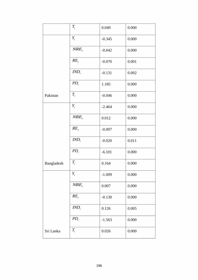
196
tT 0.049 0.000
Pakistan
tY -0.345 0.000
tNRE -0.042 0.000
tRE -0.070 0.001
tIND -0.131 0.002
tPD 1.185 0.000
tT -0.046 0.000
Bangladesh
tY -2.464 0.000
tNRE 0.012 0.000
tRE -0.007 0.000
tIND -0.020 0.011
tPD -6.101 0.000
tT 0.164 0.000
Sri Lanka
tY -1.009 0.000
tNRE 0.007 0.000
tRE -0.130 0.000
tIND 0.126 0.005
tPD -1.563 0.000
tT 0.026 0.000
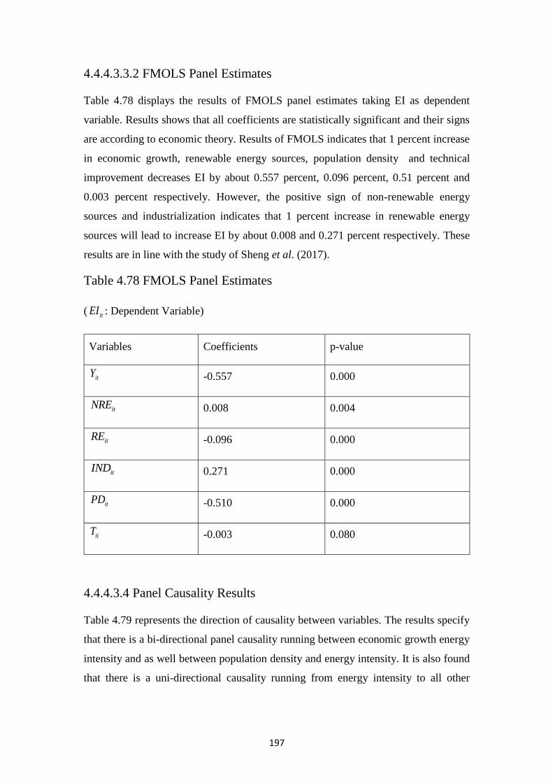
197
4.4.4.3.3.2 FMOLS Panel Estimates
Table 4.78 displays the results of FMOLS panel estimates taking EI as dependent
variable. Results shows that all coefficients are statistically significant and their signs
are according to economic theory. Results of FMOLS indicates that 1 percent increase
in economic growth, renewable energy sources, population density and technical
improvement decreases EI by about 0.557 percent, 0.096 percent, 0.51 percent and
0.003 percent respectively. However, the positive sign of non-renewable energy
sources and industrialization indicates that 1 percent increase in renewable energy
sources will lead to increase EI by about 0.008 and 0.271 percent respectively. These
results are in line with the study of Sheng et al. (2017).
Table 4.78 FMOLS Panel Estimates
( itEI : Dependent Variable)
Variables Coefficients p-value
itY -0.557 0.000
itNRE 0.008 0.004
itRE -0.096 0.000
itIND 0.271 0.000
itPD -0.510 0.000
itT -0.003 0.080
4.4.4.3.4 Panel Causality Results
Table 4.79 represents the direction of causality between variables. The results specify
that there is a bi-directional panel causality running between economic growth energy
intensity and as well between population density and energy intensity. It is also found
that there is a uni-directional causality running from energy intensity to all other
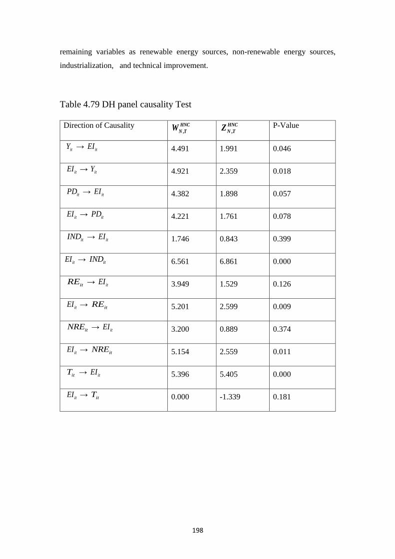
198
remaining variables as renewable energy sources, non-renewable energy sources,
industrialization, and technical improvement.
Table 4.79 DH panel causality Test
Direction of Causality ,
HNC
N TW ,
HNC
N TZ P-Value
itY → itEI 4.491 1.991 0.046
itEI → itY 4.921 2.359 0.018
itPD → itEI 4.382 1.898 0.057
itEI → itPD 4.221 1.761 0.078
itIND → itEI 1.746 0.843 0.399
itEI → itIND 6.561 6.861 0.000
itRE → itEI 3.949 1.529 0.126
itEI → itRE 5.201 2.599 0.009
itNRE → itEI 3.200 0.889 0.374
itEI → itNRE 5.154 2.559 0.011
itT → itEI 5.396 5.405 0.000
itEI → itT 0.000 -1.339 0.181
199
CHAPTER 5
SUMMARY AND CONCLUSIONS
In this chapter, we present the summary and conclusions regarding the study. We, in
detail, summarize the stated research aims and important findings here. It provides
policy recommendations based on empirical findings. It concludes with remarks about
expectations for the future researchers.
5.1 Summary and Conclusions
The fundamental objective of this research was to explore the prospects of renewable
and non-renewable energy sources in South Asian economies by utilizing the latest time
series and panel data techniques over the period 1980-2014. In this context, the study
investigated the causal relationship between both energy sources and economic growth
and also between energies and environment. Moreover, we also calculated the demand
for energy and causality between energy intensity and energy sources.
The first chapter summarizes the plan and the purpose of the study. This chapter also
gives an introduction of the task and an overview of the rationale for the research work.
In the second chapter the relevant review of literature has been discussed which
provides the better understanding of the determinants of the energy demand. This
chapter also forms the foundation for important themes and ideas used throughout the
research process. The overview provides the key factors in South Asian countries
including economic growth, renewable and non-renewable energy sources,
industrialization, population total, population density, CO2 emissions and inflation.
Chapter four provides the methodological framework of the thesis including data and
econometric measures.
Fifth chapter provides detailed methodological issues employed in the estimation of the
empirical models. The empirical work has been done in four phases consisting of two
or three models in each phase. First three models in the study explore the relationship
between economic growth, renewable energy sources, nonrenewable energy sources,
institutions and trade openness taking real gross domestic product as a dependent
variable. Fourth and fifth models explain the impact of renewable and non-renewable
energy sources on environmental quality in the presence of environmental Kuznets
curve (EKC), energy intensity, urbanization and population. Sixth and seventh models
200
determine the demand for renewable and non-renewable energy. In these models, the
future demand for both energy sources has been also forecasted for twenty years. In the
last three models, the energy intensity has been used as dependent variable.
This thesis has applied both time series and panel unit root tests to examine the
integrating properties of the variables. To examine the co-integration between
variables, Johansen likelihood based panel co-integration approaches have been
applied. The Granger causality model is applied to examine the direction of causality
between variables in selected South Asian countries. Empirical results indicates that
all variables are integrated at I(1) confirmed by panel unit root tests and the same
inference is drawn about co-integration between economic growth, trade openness and
both energy sources ( RE, NRE). The FMOLS estimation analysis reveals a positive
relationship between economic growth (Y), renewable energy sources (RE),
nonrenewable energy sources (NRE), institutions (INS) and trade openness (To). The
causality analysis confirms the existence of unidirectional panel causality from
economic growth to nonrenewable energy sources, nonrenewable energy sources to
renewable energy sources and renewable energy sources to trade openness.
The analysis which explores the relationship between environment, economic growth,
renewable energy sources, nonrenewable energy sources and population destiny has
been estimated in models 4 and 5. Using available data we applied unit root tests to
examine the integrating properties of the variables. To examine co-integration between
variables, likelihood based panel co-integration approaches have been applied. The
Granger causality are applied to examine the direction of causality between variables
in selected South Asian countries. Empirical results indicates that all variables are
integrated at I(1) confirmed by panel unit root tests and the same inference is drawn
about co-integration between environment, economic growth, population destiny and
both energy sources ( RE, NRE). The FMOLS estimation analysis reveals a positive
relationship between CO2 emissions, economic growth (Y), and non-renewable energy
sources (NRE) and population destiny (PD). Causality results provide evidence of
feedback relationship between environment and both energy sources.
Model 6 and 7 explore the determinants of demand for renewable energy sources and
nonrenewable energy sources using data of 4 South Asian countries over the period of
1980-2014. Empirical results indicates that all variables are integrated at I(1) confirmed
by unit root tests Results of FMOLS in model 6 indicate that 1 percent increase in
201
economic growth, industrialization and population total increases renewable energy
demand by about 1.228 percent, 1.230 percent, and 1.373 percent respectively. These
results show that higher per capita real income should result in greater economic
activity which in turns accelerate the use of renewable energy. The degree of
industrialization, as a measure of economic structure, is also expected to enhance the
demand for renewable energy. However, the negative sign of energy price and technical
progress indicates that 1 percent increase in energy price and technical progress will
lead to decrease renewable energy demand by about 0.004 percent and 0.020 percent
respectively. The negative sign of technical progress show that the technology is energy
saving. Results in model 7 shows that all coefficients are statistically significant and
their signs are according to economic theory. Results indicate that 1 percent increase in
economic growth, population and industrialization increases demand for non-
renewable energy sources by about 4.889 percent, 9.760 percent and 1.514 percent
respectively. However, the negative sign of energy price and technical progress
indicates that 1 percent increase in renewable energy sources will lead to decrease
nonrenewable energy demand by about 0.008 percent and 0.299 percent respectively.
This analysis in model 8 explores the relationship between energy intensity, economic
growth, renewable energy sources, nonrenewable energy sources and population
destiny. This analysis also explores the relationship between energy intensity, economic
growth, economic growth squared, urbanization, population density and trade openness
in model 9. We also applied unit root tests to examine the integrating properties of the
variables. Empirical results indicates that all variables are integrated at I(1) confirmed
by panel unit root tests and the same inference is drawn about co-integration between
environment, economic growth, population destiny and both energy sources ( RE,
NRE). The FMOLS estimation analysis reveals a negative relationship between energy
intensity, economic growth (Y), renewable energy sources (RE) and population destiny
(PD). Causality results provide evidence of feedback relationship between energy
intensity and economic growth and population density.
According to the estimated results, the final conclusion shows the positive impacts of
renewable and non-renewable energy sources on economic growth in all South Asian
countries. It is commonly known that economic growth depends on production of goods
and services while production depends directly on input like energy whether it is
202
renewable or nonrenewable. Likewise, a country with more energy has comparatively
more economic growth as compare to energy insecure countries.
5.2 Policy Recommendations
On the basis of empirical investigations and obtained results, our recommendations
includes:
The use of energy from renewable sources should be increased while the energy from
non-renewable energy sources should be decreased particularly India and Pakistan
which are the larger consumer of the energy. For the advancement of environmental
quality, the implementation of renewable energy sources in each phase of production
process can be an important factor. It is suggested that this model can be used for long
term energy policy, formation and development of renewable energy sources in future.
South Asian economies which usually dependent on foreign sources for their energy
needs, can rely on renewable energy that reduces the inclusion of foreign energy
sources and hence can reduce their energy cost and dependence. Further, considering
the escalating population in Pakistan and India this result is very alarming and calls for
prudent policy formulation.
This study suggests that there is need to explore new and efficient energy sources to
accelerate economic growth and decrease in CO2 emissions. Renewable energy sources
are environment friendly and tend to decrease CO2 emissions. In order to keep
environment clean and pollution free south Asian economies not only at regional level
but at country level need to devise the policies which promote the use of renewable
energy sources to accelerate economic growth.
This study also suggests that all south Asian countries especially India, Pakistan and
Bangladesh which are the most populous countries in the region need to slow down the
rapid urbanization process to reduce energy intensity. Energy conservation policies
should be adopted to produce more income to improve energy efficiency. In this
context, non-renewable energy sources should be replaced with renewable energy
sources.
Results shows the positive impacts of renewable energy sources on economic growth
in all South Asian countries. To get the benefits of these energy sources on economic
growth, at country level, there is need to install, operate and maintain energy from
renewable sources and encourage energy efficiency technologies. South Asian
203
countries need to formulate those policies that encourage renewable energy
development, appropriate for local conditions of economic development, social
development and resource availability. Moreover, there is need to organize public
research and development programs for a concrete reduction of energy production cost.
These programs at central level can utilize intellectuals, research instruments,
knowledge and other resources across the country. It can also provide a big picture of
progress in technology for renewable energy recourse production cost reduction.
Each South Asian country need to target energy process which include study of sectoral
demand and supply of energy, forecasting trends of various energy sources based on
economic and technological models and strategies to diversify the energy sources. For
this purpose, south Asian countries need to publish their target and include renewable
energy sources in energy mix apart from adopting energy efficiency technologies.
For the special selected South Asian economies the findings suggested that the
Government should form a vigorous policy to diminish the oil, gas and fossil fuel
consumption for electricity production, as a replacement to depend on hydro, solar and
biomass energy sources. Subsequently, the government should promote more gas
concentrated projects to alleviate the contests of gas shortage and provide it to industrial
sector at cheap cost with easy access. These such activities like switching of non-
renewable energy resources to renewable energy resources will boost the growth level
of all countries in onside and will provide pollution free environment on other side. It
will also fulfil the required energy demand in all sectors. More research efforts should
be given to the development of the renewable technologies which will be great helpful
for improving renewable energy growth as well as economic growth in the case
Bangladesh.
Finally, at regional level renewable energy can attract investment, provide energy
security through diversification, super technological research and enhance stable
economic growth. Apart from these, increasing the cost effective penetration of
renewable energy requires Considerable Corporation among decision makers of the
energy sector. Renewable energy resource exploration, evaluation, related information
system and construction of independent renewable energy system in remote areas and
islands should be encouraged in India, Pakistan and Bangladesh.
204
REFERENCES
Abbas, S. Z., Tanweer, R., Ahmad, F., ur Rasheed, F., Karim, J., & Raza, A. (2015).
Assessment of Wind Energy Potential for Small Scale Power Generation at
Thatta, Sindh, Pakistan. Journal of Basic & Applied Sciences,11, 261.
Adjaye, J. A. (2000). The relationship between energy consumption, energy prices and
economic growth: time series evidence from Asian developing countries.
Energy Economics, 22: 625-625.
Ahmad, Md. Mansur. (2012) Openness, Institutions, and Economic Growth: Empirical
Evidence from Panel Estimation: Master Dissertation.
Ahmad, N., Shahbaz, M. & Kyophilavong, P. (2016). Revisiting the emissions-energy-
trade nexus: evidence from the newly industrializing countries. Environmental
Science and Pollution Research.
Ahmed, M, M., and Koji Shimada, K. (2019). The Effect of Renewable Energy
Consumption on Sustainable Economic Development: Evidence from
Emerging and Developing Economies, Energies, 12, 2954
Ahmed, S., Mahmood, A., Hasan, A., Sidhu, G.A.S., & Butt, M.F.U. (2016). A
comparative review of China, India and Pakistan renewable energy sectors and
sharing opportunities. Renewable and Sustainable Energy Reviews, 57, 216-
225.
Aïssa, M. S. B., Jebli, M.B. & Youssef, S.B. (2014). Output, Renewable Energy
Consumption and Trade in Africa. Energy Policy, 66: 11-18.
Akarca, A.T., Long, T.V., (1979). Energy and employment: a time series analysis of
the causal relationship. Resource Energy 5, 326–331.
Akarca, A.T., Long, T.V., (1980). On the relationship between energy and GNP: a re -
examination. Journal of Energy and Development. 5, 326–331.
Akinlo, A. E. (2008), “Energy Consumption and Economic Growth: Evidence from 11
Sub-Sahara African Countries”, Energy Economics, Vol. 30, pp. 2391-2400.
Alam, M. J., Begum, I. A., Buysse, J., Rahman, S. and Huylenbroeck, G. V. (2011).
“Dynamic modeling of causal relationship between energy consumption, CO2

205
emissions and economic growth in India”, Renewable and Sustainable Energy
Reviews, Vol.15: 3243-3251.
Alam, M.J., Begum, I.A., Buysse, J., & Huylenbroek, G.V. (2012). Energy
consumption, carbon emissions, and economic growth nexus in Bangladesh:
Co-integration and dynamic causality analysis. Energy Policy 45 217-225.
Alam.S, Fatima. A, Butt.M.S (2007) Sustainable development in Pakistan in the content
of energy consumption demand and environmental degradation. Journal of
Asians Economics 18 (2007)825-837
Ali, G., Bashir, M. K., Ali, H., & Bashir, M. H. (2016). Utilization of rice husk and
poultry wastes for renewable energy potential in Pakistan: An economic
perspective. Renewable and Sustainable Energy Reviews, 61, 25-29.
Al-Mulali U, Ozturk I (2016). The investigation of environmental Kuznets curve
hypothesis in the advanced economies: the role of energy prices. Renewable and
Sustainable Energy Reviews 54:1622–1631
Al-Mulali, U., Fereidouni, H.G. & Lee, J.Y. (2014). Electricity Consumption from
Renewable and Non-Renewable Sources and Economic Growth: Evidence from
Latin American Countries. Renewable and Sustainable Energy Reviews, 30:
290-298.
Al-Mulali, U., Fereidouni, H.G., Lee, J.Y., Sab, C.N.B.C. (2013). Examining the Bi-
Directional Long Run Relationship between Renewable Energy Consumption
and GDP Growth. Renewable and Sustainable Energy Reviews, 22: 209–222.
Altinay, G and E. Karagol, (2004) Structural break, unit root and the casualty between
energy consumption and GDP in Turkey. Energy Economics 26, 985-994.
Altinay, G and E. Karagol, (2005) Electricity consumption and economic growth:
Evidence from Turkey. Energy Economics 27, 849-856.
Amer, M., & Daim, T.U. (2011). Selection of renewable energy technology for a
developing country: A case of Pakistan. Energy for Sustainable Development
15 (4) 420-435.
Amirat, A., Bouri, A. (2010), Energy and Economic Growth: The Algerian Case.
206
Ang, J.B. (2007). “CO2 emissions, energy consumption, and output in France.” Energy
Policy, Vol. 35, pp. 4772-4778.
Antweiler, Werner, Brian R. Copeland and M. Scott Taylor.(2001). "Is Free Trade
Good for the Environment?." American Economic Review, 91(4):877-908.
Apergis, N. & Danuletiu, D.C. (2014). Renewable Energy and Economic Growth:
Evidence from the Sign of Panel Long-Run Causality. International Journal of
Energy Economics and Policy, 4(4): 578-587.
Apergis, N. & Eleftheriou, S. (2015). Renewable Energy Consumption, Political and
Institutional Factors: Evidence from a Group of European, Asian and Latin
American Countries. The Singapore Economic Review, 60(1): 1550008 (19
pages).
Apergis, N. & Payne, J.E. (2010a). Renewable Energy Consumption and Economic
Growth: Evidence from a Panel of OECD Countries. Energy Policy, 38: 656–
660.
Apergis, N. & Payne, J.E. (2010b). Renewable Energy Consumption and Growth in
Eurasia. Energy Economics, 32: 1392-1397.
Apergis, N. & Payne, J.E. (2011a). The Renewable Energy Consumption–Growth
Nexus in Central America. Applied Energy, 88: 343-347.
Apergis, N. & Payne, J.E. (2011b). On the Causal Dynamics between Renewable and
Non Renewable Energy Consumption and Economic Growth in Developed and
Developing Countries. Energy Syst., 2: 299-312.
Apergis, N. & Payne, J.E. (2011c). Renewable and Non-Renewable Electricity
Consumption Growth Nexus: Evidence from Emerging Market Economies.
Applied Energy, 88: 5226-5230.
Apergis, N. & Payne, J.E. (2012a). Renewable and Non-Renewable Energy
Consumption Growth Nexus: Evidence from a Panel Error Correction Model.
Energy Economics, 34:733-738.
Apergis, N. & Payne, J.E. (2012b). The Electricity Consumption-Growth Nexus:
Renewable Versus Non-Renewable Electricity in Central America. Energy
Sources, (7):423-431.
207
Apergis, N. & Payne, J.E., Menyah, K. & Rufael, Y.W. (2010). On the Causal
Dynamics between Emissions, Nuclear Energy, Renewable Energy, and
Economic Growth. Ecological Economics, 69: 2255-2260.
Apergis, N. (2016). Environmental Kuznets Curves: New Evidence on both Panel and
Country Level CO2 Emissions. Energy Economics, 54: 263-271.
Apergis, N. and Payne, J.E. (2009). “CO2 emissions, energy usage, and output in
Central America.” Energy Policy, Vol. 37, pp. 3282-3286.
Apergis, N., & Payne, J.E. (2009). Energy consumption and economic growth in
Central America: Evidence from panel co-integration and error correction
model. Energy Policy 31 (2) 211-216.
Apergis, N., & Payne, J.E. (2010a). Renewable energy consumption and economic
growth: Evidence from a panel of OECD countries. Energy Policy, 38(1), 656-
660.
Apergis, N., & Payne, J.E. (2010b). Renewable energy consumption and growth in
Eurasia. Energy Economics, 32(6), 1392-1397.
Apergis, N., Payne, J.E. (2012). Renewable and non-renewable energy consumption-
growth nexus: Evidence from a panel error correction model. Energy
Economics, 34(3), 733-738.
Apergis, N.; Payne, J.E.(2010). Renewable energy consumption and economic growth:
Evidence from a panel of OECD countries. Energy Policy, 38, 656–660.
Apergis, N.; Payne, J.E.(2014). The causal dynamics between renewable energy, real
GDP, emissions and oil prices:evidence from OECD countries. Appl. Econ, 46,
4519–4525.
Aqueel, A., and M. S. Butt, (2001) The Relationship between Energy consumption and
Economic Growth in Pakistan, Asia-Pacific Development Journal 8:2
(December), 101-110.
Ara Begum.R, Sohag.K,Abdullah.S.M.S, Jaffar.M (2015) CO2 emission,energy
consumption,economic and population growth in Malaysia.Renewable and
sustainable energy review 41(2015)594-601
208
Arouri, M.E.H., Youssef, A.B., M’henni, H., Rault.C. (2012). Energy consumption,
economic growth, and 𝐶𝑂2 emissions in Middle East and North African
countries. Energy Policy 45 342-349.
Arvin. M.B,Pradhan.R.P , Norman.N.R (2015). Transportation intensity, urbanization,
economic growth, and CO2 emission in the G-20 countries. Utilities policy 35
(2015) 50-66
Asghar Z., (2008). Energy-GDP relationship: a casual analysis for the five countries of
South Asia. Applied Econometrics and International Development. 8, 167–180.
Asghar, Z. Rahat, T. (2011). Energy-GDP relationship: a casual analysis for Pakistan:
A gragh Thoretic Approach. Applied Econometrics and International
Development. 11: 205–214.
Azam, M., & Khan, A. Q. (2015). Urbanization and environmental degradation:
Evidence from four SAARC Countries—Bangladesh, India, Pakistan, and Sri
Lanka. Environmental Progress & Sustainable Energy.
Baek J, Pride D (2014). On the income–nuclear energy–CO2 emissions nexus revisited.
Energy Econ 43:6–10
Baky,M, A, H., Md. Mustafizur Rahman,M, M., Islam, A,K,M, S., (2017).
Development of renewable energy sector in Bangladesh: Current status and
future potentials, Renewable and Sustainable Energy Reviews, 73: 1184–1197
Baran, B., Mamis, M. S., &Alagoz, B. B. (2016). Utilization of energy from waste
potential in Turkey as distributed secondary renewable energy
source.Renewable Energy, 90, 493-500.
Basher, S. A. & Westerlund, J. (2009). Panel cointegration and the monetary exchange
rate model, Economic Modelling, 26, 506-513.
Beck, Thorsten, and Ross Levine (2004), Stock markets, banks, and growth: Panel
evidence, Journal of Banking and Finance 28: 423-442
Belke, A., Dobnik, F., Dreger, C., 2011. Energy consumption and economic growth:
New insights into the cointegration relationship. Energy Econ. 33, 782–789.
209
Belloumi.M,Alshehry.A.S (2016) The impact of urbanization on energy intensity in
Saudi Arabia.Sustainability,8,375
Bento JPC, Moutinho V (2016) CO2 emissions, non-renewable and renewable
electricity production, economic growth, and international trade in Italy. Renew
Sust Energ Rev 55:142–155
Bentzen, J., & Engsted, T. (1993). Short-and long-run elasticities in energy demand: a
cointegration approach. Energy Economics, 15 (1), 9-16.
Bernardini, O., Galli, R., 1993.Dematerialization: long term trends in the intensity of
use of materials and energy. Futures 431–448 (May).
Berndt, E.R., Kolstad, C. & Lee, J. (1993). Measuring the Energy Efficiency and
Productivity Impacts of Embodied Technical Change, Energy Journal, vol. 14,
pp. 33-55.
Bernstein, R., & Madlener, R. (2015). Short- and long-run electricity demand
elasticities at the subsectoral level: A cointegration analysis for German
manufacturing industries. Energy Economics, 48, 178–187.
Bhattacharya M, Paramati S R, Ozturk I, Bhattacharya S. (2016). The effect of
renewable energy consumption on economic growth: evidence from top 38
countries. Appl Energy 162: 733–41.
Bhattacharya, M., A. S. Churchill, and S. R. Paramati. (2017). The dynamic impact of
renewable energy and institutions on economic output and CO2 emissions
across regions. Renewable Energy, 111:157–67.
Bhattacharya, M., S. R. Paramati, I. Ozturk, and S. Bhattacharya. (2016). The effect of
renewable energy consumption on economic growth: evidence from top 38
countries. Applied Energy, 162:733–41
Bilan, Y.; Streimikiene, D.; Vasylieva, T.; Lyulyov, O.; Pimonenko, T.; Pavlyk, A.
(2019). Linking between Renewable Energy, CO2 Emissions, and Economic
Growth: Challenges for Candidates and Potential Candidates for the EU
Membership. Sustainability, 11, 1528.
Bildirici, M.E.(2014) Relationship between biomass energy and economic growth in
transition countries: Panel ARDL approach. GCB Bio Energy, 6, 717–726.
210
Bildirici, M.E.(2014) Relationship between biomass energy and economic growth in
transition countries: Panel ARDL approach. GCB Bio Energy, 6, 717–726.
Bilgili F, Kocak E, Bulut U (2016). The dynamic impact of renewable energy
consumption on CO2 emissions: a revisited Environmental Kuznets Curve
approach. Renew Sust Energ Rev 54:838–845
Bilgili, F. & Ozturk, I. (2015). Biomass Energy and Economic Growth Nexus in G7
Countries: Evidence from Dynamic Panel Data. Renewable and Sustainable
Energy Reviews, 49: 132-138.
Bittencourt, Manoel (2010), Financial development and economic growth in Latin
America: Is Schumpeter right? Working Paper 191, University of Pretoria.
Bölük, G. & Mert, M. (2014). The Renewable Energy and Growth: Evidence for Turkey
using Environmental Kuznets Curve Model. The WEI International Academic
Conference Proceedings, The West East Institute, Budapest, Hungary
Bowden, N. & Payne, J.E. (2010). Sectoral Analysis of the Causal Relationship
between Renewable and Non-Renewable Energy Consumption and Real Output
in the US. Energy Sources, B(5): 400-408.
Breitung, J. (2005). A Parametric Approach to the Estimation of Cointegrating Vectors
in Panel Data, Econometric Reviews, 24(2): 151-173.
Bremner, J., López-Carr, D., Suter, L., & Davis, J. (2010). Population, poverty,
environment, and climate dynamics in the developing world.Interdisciplinary
Environmental Review, 11(2-3), 112-126.
Breusch, T.S & Pagan A.R. (1980). The Lagrange Multiplier Test and Its Applications
to Model Specification Tests in Econometrics, Review of Economic Studies, 47:
239-53.
Burke.P, J., & Liao, H. (2015). Is the price elasticity of demand for coal in China
increasing?. China Economic Review , 36, 309-322.
Canning, D., and Pedroni, P., (2008). Infrastructure, long-run economic growth and
causality tests for cointegrated panels. Manchester School, 76, 504-
527.Economics 19, 435-444.
211
Carlino, G. A., Chatterjee, S., & Hunt, R. M. (2007). Urban density and the rate of
invention. Journal of Urban Economics, 61(3), 389-419.
Carrion-I-Silvestre, Josep Lluis, Barrio-Castro, Tomas Del and lopez-Bazo, Enrique,
(2005). Breaking the Panels: An Application to the GDP Per Capita,
Econometrics Journal, 8: 159-175.
Cetin.M,Ecevit.E(2015) Urbanization,Energy Consumption and CO2 Emissions in
Sub-Sahara Countries:A panel Cointegration and Causality Analysis. Journal
of Economics and Development studies,Vol.3,No.2,pp.66-76
Chandio, A, A., Rauf, A., Jiang,Y.,Ozturk, I and Ahmad , F. (2019). Cointegration and
Causality Analysis of Dynamic Linkage between Industrial Energy
Consumption and Economic Growth in Pakistan, Sustainability, 11, 4546
Chang, C.C. (2010). A multivariate causality test of carbon dioxide emission, energy
consumption and economic growth in China. Applied Energy, 87(11),
3533-3537.
Chaudhry, A. A. (2010). A Panel Data Analysis of Electricity Demand in Pakistan. The
Lahore Journal of Economics, 15, 75-106.
Chaudhry, I.S., Farooq, F., Nasim, I. (2015). Long run panel data analysis of energy
consumption and real GDP of south Asian economies. Pakistan journal
of social sciences, 35(2), 715-727.
Chaudhry, M.A., Raza, R., & Hayat, S.A. (2009). Renewable energy technologies in
Pakistan: Prospects and challenges. Renewable and Sustainable Energy
Reviews 13 (6) 1657-1662.
Chaudhry, Q. Z. (2007). An Investigation of Wind Power Potential of Gharo, Sindh,
Pakistan. Pak J Metrol, 6(11), 1-6.
Chaudhry, T. (2010). Estimating Residential Electricity Demand Responses in
Pakistan’s Punjab. The Lahore Journal of Economics, 15 ,107-138.
Chen, J. H., & Huang, Y. F. (2013). The study of the relationship between carbon
dioxide (CO2) emission and economic growth. Journal of International and
Global Economic Studies, 6(2), 45-61.
212
Cheng, B.S. and T.W.Lai, (1997) An investigation of cointegration and causality
between energy consumption and economic activity in Tiwan. Energy
Chien T, Jin-Li H. Renewable energy: an efficient mechanism to improve GDP. Energy
Policy 2008;36(8):3045–52.
Chiu CL, Chang TH (2009). What proportion of renewable energy supplies is needed
to initially mitigate CO2 emissions in OECD member countries? Renew Sust
Energ Rev 13(6):1669–1674
Cho, S.; Heo, E.; Kim, J (2015). Causal relationship between renewable energy
consumption and economic growth: Comparison between developed and less-
developed countries. Geosyst. Eng. 18, 284–291.
Choi, I. (2001). Unit Roots Tests for Panel Data, Journal of International Money and
Finance 20: 229-272.
Christopher, M. C. (2007) Intensity of Energy Use in the USA. 1949-2003. Journal of
Business and Economics Research, Vol. 5 November 11
Connoly, D., Lund, H., Mathiesen, B.V., & Leahy, M. (2010). A review of computer
tools for analyzing the integration of renewable energy into various energy
systems. Applied Energy, 87(4), 1059-1082.
Creutzig.F,Baiocchi.G,Bierkandt.R,Pichler.P.P,Seto.K.C (2015) Global typology of
urban energy use and potentials for an urbanization mitigation
wedge.PNAS,Vol.112,No.20,6283-6288
Crotte, A., Noland. R. B & Graham. D. J. (2010). An analysis of gasoline demand
elasticities at the national and local levels in Mexico. Energy Policy, 38(8), 4445-
4456.
Dagher, L. (2012). Natural gas demand at the utility level: an application of dynamic
elasticities. Energy Economics, 34(4), 961-969.
Dai.D,Liu.H (2011) An empirical Reasearch and STIRPAT model analysis of
urbanization and CO2 emission in China.Advanced in information sciences and
services sciences.Vol.3.
213
Darmstadter, J.: Dunkerley, J.: and Alterman, J. 1977. How Industrial Societies Use
Energy. A Comparative Analysis. Published for Resources for the Future by the
Johns Hopkins University Press.
De Ridder, K., Lefebre, F., Adriaensen, S., Arnold, U., Beckroege, W., Bronner, C., ...
& IntPanis, L. (2008). Simulating the impact of urban sprawl on air quality and
population exposure in the German Ruhr area. Part I: Reproducing the base
state. Atmospheric Environment, 42(30), 7059-7069.
Dedeoğlu, D., Kaya, H., 2013. Energy use, exports, imports and GDP: New evidence
from the OECD countries. Energy Policy, 57, 469-476.
Destek, M A (2018). Financial development and energy consumption nexus in
emerging economies, ENERGY SOURCES, PART B: ECONOMICS,
PLANNING, AND POLICY, VOL. 13, NO. 1, 76–81
Dogan E, Seker F (2016b) Determinants of CO2 emissions in the European Union: the
role of renewable and non- renewable energy. Renew Energy 94:429–439
Dogan E, Seker F (2016c). The influence of real output, renewable and non-renewable
energy, trade and financial development on carbon emissions in the top
renewable energy countries. Renew Sustain Energy Rev 60:1074–1085
Dogan E. (2015). The relationship between economic growth and electricity
consumption from renewable and non-renewable sources: a study of Turkey.
Renew and Sustain Energy Review 52:534–46.
Drechsel.P,Gyiele.L,Kunze.D,Cofie.O(2001) Population density,Soil nutrient
depletion and economic growth in Sub Saharan Africa. Ecological Economics
38(2001) 251-258
Emmanuel, N. and Ebi, B.O. (2013), Institutional quality, petroleum resources and
economic growth: A difference in differences approach using Nigeria, Brazil
and Canada. International Journal of Humanities and Social Science, 3(20),
198-206.
Erdal, G., Erdal,H., & Esengun, K. (2008). The causality between energy consumption
and economic growth in Turkey. Energy Policy 36 (10) 3838-3842.
214
Eris, M.N; Ulasan, B., 2013.Trade openness and economic growth: Bayesian model
averaging estimate of cross-country growth regressions. Economic Modelling
33: 867–883
Fan, S., & Hyndman, R. J. (2011). The price elasticity of electricity demand in South
Australia. Energy Policy, 39(6), 3709-3719.
Fan.Y,Liu.L.C,Wu.G,Wei.Y.M (2006) Analyzing impact factor of CO2 emission using
the STRIPAT model. Environmental impact Assessment Review 26(2006)377-
395
Fang, Y. (2011). Economic Welfare Impacts from Renewable Energy Consumption:
The China Experience. Renewable and Sustainable Energy Reviews, 15: 5120-
5128.
Farhani. S, Ozturk .I (2015) causal relationship between CO2 emission, real GDP,
energy consumption,trade oppeness, financial development and urbanization in
Tunisia. Environ Sci pollut Res (2015) 22: 15663-15676
Farooq, M. K., & Kumar, S. (2013). An assessment of renewable energy potential for
electricity generation in Pakistan. Renewable and Sustainable Energy
Reviews, 20, 240-254.
Fouquet, R., Pearson, P., Hawdon, D., Robinson, C. & Stevens, P. 1997, "The Future
of UK Final User Energy Demand", Energy Policy, vol. 25, no. 2, pp. 231-240.
Frederiksen, p., 1981. Further Evidence on the Relationship between Population
Density and Infrastructure: The Philippines and Electrification, Economic
Development and Cultural Change, Vol. 29, No. 4 (Jul., 1981), pp. 749-758
Galindo, L. M. (2005), “Short- and Long-run Demand for Energy in Mexico: A Co-
integration Approach”, Energy Policy, Vol. 33, pp. 1179-1185.
Galli, R. (1988). “The Relationship between Energy Intensity and Income Levels:
Forecasting Long Term Energy Demand in Asian Emerging Countries.” The
Energy Journal, (19)4: 85-105.
Gbadebo, O.O. and Okonkwo, C. (2009), Does energy consumption contribute to
economic performance? Empirical evidence from Nigeria. Journal of
Economics and International Finance, 1(2), 44-58.
215
Ghafoor, A., urRehman, T., Munir, A., Ahmad, M., & Iqbal, M. (2016). Current status
and overview of renewable energy potential in Pakistan for continuous energy
sustainability. Renewable and Sustainable Energy Reviews, 60, 1332-1342.
Ghali, K. H. and M. I. T. EI-S akka, (2004) Energy use and output growth in Canada:
a multivariable co-integration analysis. Energy Economics 26, 225-238.
Ghosh, S., (2000) Electricity consumption and economic growth in India. Energy
Policy 30, 125-129.
Ghosh.S,Kanjilal.K(2014) Long term equilibrium relationship between energy
consumption,urbanization and economic activity: Emperical evidence from
india. Energy 66(2014) 324-333
Ghosh.S,Kanjilal.K(2014) Long term equilibrium relationship between energy
consumption,urbanization and economic activity: Emperical evidence from
india. Energy 66(2014) 324-333
GOP, Pakistan Economic Survey 2009-10, Economic Advisor’s Wing, Minis- try of
Finance, Government of Pakistan (GOP), Islamabad.
Guan.X,Zhou.M (2015) Decomposing the effecting factors of urbanization on energy
consumption of china.The open cybernetics&Systemics Journal,2015,9,2035-
2043
Habibullah. M., Masjuki. H., H. Kalam. M.A., Rahman. S. A., Mofijur, M., Mobarak.
H. M.,&Ashraful.A. M. (2015). Potential of biodiesel as a renewable energy
source in Bangladesh. Renewable and Sustainable Energy Reviews, 50, 819-
834.
Hadri, K. (2000). Testing for Stationarity in Heterogenous Panels, Econometrics
Journal, 3: 148-161.
Halder, P. K., Paul, N., Joardder, M. U. H., &Sarker, M. (2015). Energy scarcity and
potential of renewable energy in Bangladesh. Renewable and Sustainable
Energy Reviews, 51, 1636-1649.
Halicioglu, F. (2009) “An Econometric Study of CO2 Emissions, Energy Consumption,
Income and Foreign Trade in Turkey”, Energy Policy, Vol.37, pp.1156-1164.
216
Halicioglu, F. (2011). A dynamic study of income, energy and exports in Turkey.
Halkos, G.E. & Tzeremes, N.G. (2014). The Effect of Electricity Consumption from
Renewable Sources on Countries' Economic Growth Levels: Evidence from
Advanced, Emerging and Developing Economies. Renewable and Sustainable
Energy Reviews, 39: 166-173.
Hamilton, J. D. (2011). Historical oil shocks (No. w16790). National Bureau of
Economic Research.
Heidari.H,Katircioglu.S.T,Saeid pour.L(2015) Economic growth,CO2 emission and
energy consumption in the five ASEAN Countries. Electrical power and energy
system 64(2015)785-791
Hislop, D., (1992) Energy Options, an introduction to small scale renewable energy
technologies, International Tech Publications Ltd, London, p. 103-105.
Ho, C. Y and K, W. Siu, (2006) A dynamic equilibrium of electricity consumption and
GDP in Hong Kong: An empirical investigation. Energy Policy 35, 2507-2513.
Hondroyiannis, G., S. Lolos and E. Papapetrou (2002), “Energy Consumption and
Economic Growth: Assessing the Evidence from Greece”, Energy Economics,
Vol. 24, pp. 319-336.
Hossain, Md. S., 2012. Multivariate Granger causality between economic growth,
electricity consumption, exports and remittances for the panel of three SAARC
countries. Global Journal of Management and Business Research, 12, 41-54.
Hossain, S. (2012). An econometric analysis for CO 2 emissions, energy consumption,
economic growth, foreign trade and urbanization of Japan.
Hossain.M.S(2011) Panel estimation for CO2 emission, energy consumption ,economic
growth,trade oppeness and urbanization of newly industrialization
countries.Energy policy 39(2011)6991-699.
Hungary Bowden, N. & Payne, J.E. (2010). Sectoral Analysis of the Causal
Relationship between Renewable and Non-Renewable Energy Consumption
and Real Output in the US. Energy Sources, B (5): 400-408.
217
Hunt, L.C. & Ninom iya, Y. 2005, "Primary Energy Demand in Japan: An Empirical
Analysis of Long-Term Trends and Future CO2 Emissions", Energy Policy, vol.
33, no. 11, pp. 1409-1424.
Hurlin.C,Venet.B(2008) Financial development and growth:A Re-Examination using a
panel granger causality test.
Im, K., Pesaran H. & Shin Y. (2003). Testing for Unit Roots in Heterogenous Panels,
Journal of Econometrics, 115(1): 53-74.
International Energy Agency, 2007. World energy outlook, IEA, Paris.
Irfan. M, Shaw. K (2015) modeling the effect of energy consumption and urbanization
on environmental pollution in South Asian countries: a non-parametric panel
approach.Qual Quant Dolro.1007/s 11135-015-0294-X
Irfan. M, Shaw. K (2015) modeling the effect of energy consumption and urbanization
on environmental pollution in South Asian countries: a non-parametric panel
approach.Qual Quant Dolro.1007/s 11135-015-0294-X
Iyoboyi, M. and Latifah, M.P. (2014), Institutional capacity and macroeconomic
performance: Empirical evidence from Nigeria. Research in Applied
Economics, 6(1), 38-60.
Jabeur, B, S.(2019) The Relationship Between Renewable Energy Consumption and
Economic Growth in France: a Necessary Condition Analysis. Environ Model
Assess.
Jafari.Y, Othman .J, Mohdnor.A.H.S (2012) energy consumption, economic growth
and environmental pollutants in Indonesia. Journal of policy modeling 34
(2012) 879 – 889
Jalil, A and Feridum, M. (2011). Impact of financial development on economic growth:
empirical evidence from Pakistan, Journal of the Asia Pacific Economy, Vol.
16(1), pp 71-80
Jalil, A. and Mahmud, S. F. (2009). “Environment Kuznets curve for CO2 emissions: a
cointegration analysis”, Energy Policy, Vol. 37, pp. 5167-5172.
218
Jamil, F., & Ahmad, E. (2011). Income and price elasticities of electricity demand:
Aggregate and sector-wise analyses. Energy Policy, 39(9), 5519-5527.
Jebli, M.B. & Youssef, S.B. (2015). Economic Growth, Combustible Renewables and
Waste Consumption, and CO2 Emissions in North Africa. Environ Sci Pollut
Res, published online 12 June.
Jebli, M.B., Youssef, S.B. & Ozturk, I. (2015). The Role of Renewable Energy
Consumption and Trade: Environmental Kuznets Curve Analysis for Sub-
Saharan Africa Countries. African Development Review, 27(3): 288-300.
Jebli, M.B., Youssef, S.B., Ozturk, I. (2016), Testing environmental Kuznets Curve
hypothesis: The role of renewable and non-renewable energy consumption and
trade in OECD countries. Ecological Indicators, 60, 824-831.
Johansen, S. 1995. Likelihood-Based Inference in Cointegrated Vector Autregressive
Models. Oxford: Oxford University Press.
Johansson. T.B., McCormick. K., Neij, L., &Turkenburg. W. (2004). The potentials of
renewable energy, 25, March.
Jones, D.W., 1989. Urbanization and energy use in economic development. Energy J.
10, 29–44.
Judson, R.A., R. Schmalensee and T.M. Stoker (1999). “Economic Development and
the Structure of the Demand for Commercial Energy.” The Energy Journal,
(20)2: 29-57.
Kahia, M., Ben Jebli, M. & Belloumi, M. (2019). Analysis of the impact of renewable
energy consumption and economic growth on carbon dioxide emissions in 12
MENA countries. Clean Technology and Environmental Policy, 21, 871–885.
Kahouli, B., (2017). The short and long run causality relationships among economic
growth, energy consumption and financial development: Evidence from South
Mediterranean Countries (SMCs). Energy Economics. 68, 19–30.
Kahouli, B., (2018). The causality link between energy electricity consumption, CO2
emissions, R & D Stock and Economic Growth in Mediterranean Countries.
Energy. 145, 388–399.
219
Kahouli, B., (2019). Does static and dynamic relationship between economic growth
and energy consumption exist in OECD countries? Energy Reports, 5, 104–116
Kahsai, M.S., Nondo, C., Schaeffer, P.V., Gebremedhin, T.G., 2012. Income level and
the energy consumption-GDP nexus: Evidence from Sub-Saharan Africa.
Energy Econ. 34 (3), 739–746.
Karatayev, M., & Clarke, M. L. (2014). Current energy resources in Kazakhstan and
the future potential of renewables: A review. Energy Procedia, 59, 97-104.
Kashman. A, Duman. Y.S (2015) CO2 emission, economic growth, energy
consumption, trade and urbanization in new EU member and candidates
countries: A panel data analysis. Economic Modeling 44(2014)97-103
Kasman, A., Duman, Y.S., 2015. CO2 emissions, economic growth, energy
consumption, trade and urbanization in new EU member and candidate
countries: A panel data analysis. Econ. Model. 44, 97–103.
Kaygusuz, K., 2007. Energy for sustainable development: key issues and challenges.
Energy Sources, Part B: Economics, Planning, and Policy 2, 73–83.
Kaygusuz, K., Yuksek, O., Sari, A., 2007. Renewable energy sources in the European
Union: markets and capacity. Energy Sources, Part B: Economics, Planning,
and Policy 2, 19–29.
Keyhani. A., Ghasemi-Varnamkhasti.M., Khanali , M. &Abbaszadeh, R. (2010). An
assessment of wind energy potential as a power generation source in the capital
of Iran, Tehran. Energy, 35(1), 188-201.
Khobai H, Roux P Le (2017) The relationship between energy consumption, economic
growth and carbon dioxide emission: the case of South Africa. Int J Energy
Econ Policy 7(3):102–109
Kraft, J., Kraft, A., (1978). On the relationship between energy and GNP. Journal of
Energy Development. 3, 401–403.
Kronenberg(2009) The impact of demographic change on energy use and greenhouse
gas emission in Germany. Ecological Economics 68(2009) 2637-2645
220
Kumar, A., Kumar, K., Kaushik, N., Sharma, S., & Mishra, S. (2010). Renewable
energy in India: current status and future potentials. Renewable and Sustainable
Energy Reviews, 14(8), 2434-2442.
Kumar, S. (2016). Assessment of renewables for energy security and carbon mitigation
in Southeast Asia: The case of Indonesia and Thailand. Applied Energy, 163,
63-70.
Kumar, S., &Madlener, R. (2016). CO 2 emission reduction potential assessment using
renewable energy in India. Energy, 97, 273-282.
Kurbatova, T. &Khlyap, H. (2015). State and economic prospects of developing
potential of non-renewable and renewable energy resources in
Ukraine. Renewable and Sustainable Energy Reviews, 52, 217-226.
Kuznets, S. (1971). Economic Growth of Nations: Total Output and Production
Structure. Cambridge, MA: The Belnapp Press of Harvard University.
Latif, A., &Ramzan, N. (2014) Review of Renewable Energy Resources in Pakistan.
Journal of Global Innovations in Agricultural and Social Sciences, 2 (3), 127-
132.
Lean, H.H., Smyth, R., (2010). On the dynamics of aggregate output, electricity
consumption and exports in Malaysia: evidence from multivariate Granger
causality tests. Appl. Energy 87, 1963–1971.
Lee, C. C. and C. P. Chang, (2008) Energy consumption and economic growth in Asian
economies a more comprehensive analysis using panel data. Energy Economics
30, 50-65.
Lee, C. C., & Lee, J. D. (2010). A panel data analysis of the demand for total energy
and electricity in OECD countries, The Energy Journals, 31, 1-23.
Lee, C. C., (2005) Energy consumption and DGP in developing countries: a
cointegrated panel analysis. Energy Economics 27, 415-427.
Levin, A., Lin C.F. & Chu C.S.J. (2002). Unit Root Tests in Panel Data: Asymptotic
and Finite Sample Properties, Journal of Econometrics.
221
Li, F., Dong, S., LI, X., Liang, Q., & Yang, W. (2011). Energy consumption-economic
growth relationship and carbon dioxide emissions in china. Energy Policy 39
(2) 568-574.
Li, K., Fang, L., He, L. (2018). How urbanization affects China's energy efficiency: A
spatial econometric analysis, Journal of Cleaner Production 200: 1130-1141
Li.B,Yao.R(2009) Urbanization and its impact on building energy consumption and
efficiency in China. Renewable Energy 34(2009)1994-1998
Li.K, Lin.B (2015) Impact of urbanization and industrialization on energy consumption
/CO2 emissions: Does the level of development matter? Renewable and
sustainable Energy Review 52(2015)1107-1122.
Li.K, Lin.B (2015) Impact of urbanization and industrialization on energy consumption
/CO2 emissions: Does the level of development matter? Renewable and
sustainable Energy Review 52(2015)1107-1122.
Liddle.B(2014) impact of population,age structure and urbanization on carbon
emiossion/energy consumption: Evidence from macro-level, cross- country
analyses. Popular Environ (2014) 35:286-304
Liddle.B,Lung.S (2010) Age-structure,urbanization and climate change in developed
countries:revisiting STRIPAT for disaggregated population and consumption
related environmental impacts.Popular Environ(2010) 31:317-343
Lim, K. M., Lim, S. Y., & Yoo, S. H. (2014). Short-and long-run elasticities of
electricity demand in the Korean service sector. Energy Policy, 67, 517-521.
Lin, B.Q. (2003). Electricity Demand in the People's Republic of China: Investment
Requirement and Environmental impact, ERD Working Paper Series,
Economics and Research Department, Asian Development Bank.
Lin, C. Y. C. (2011). Estimating supply and demand in the world oil market. Journal
of Energy and Development, 34 (1), 1-32.
Lin.B,Lin.H(2015) China building energy efficiency and urbanization. Energy and
building 86(2015)356-365
222
Liu, G. (2004). Estimating energy demand elasticities for OECD countries. A dynamic
panel data approach.
Liu, W., Lund, H., Mathiesen, B. V., & Zhang, X. (2011). Potential of renewable energy
systems in China. Applied Energy, 88(2), 518-525.
Liu, X. Meng, C. Tam, (2015) Building information modelling based building design
optimization for sustainability, Energy Build. 105 (1) 139–153.
Liu.Y (2009) exploring the relationship between urbanization and energy consumption
in China using ARDL (autoregressive distribution lag) and FDM (factor
decomposition model). Energy 34 (2009) 1846-1854
Liu.Y, Yamauchi. F (2014) Population density, migeration and return to human capital
and lanfd:Insight from Indonesia. Food policy 48(2014) 182-193
Liu.Y,Yamauchi.F (2014) Population density,migeration and return to human capital
and lanfd:Insight from Indonesia. Food policy 48(2014) 182-193
Lu, M.-J., C.-Y. C. Lawell, and S. Chen. (2017). The effects of energy policies in China
on GDP, industrial output, and new energy profits. Working Paper.
Lund, H. (2007). Renewable energy strategies for sustainable development. Energy,
32(6), 912-919.
Lund.H., & Mathiesen.B.V. (2009). Energy system of 100% renewable energy
systems-The case of Denmark in years 2030 and 2050. Energy, 34(5), 524-531.
Ma, H., Oxley, L., Gibson, J., & Li, W. (2010). A survey of china’s renewable energy
economy. Renewable and Sustainable Energy Reviews, 14(1), 438-445.
Maddala, G.S. & Wu, S. (1999). A Comparative Study of Unit Root Tests with Panel
Data and a New Simple Test, Oxford Bulletin of Economics and Statistics, 61:
631-652.
Mahadevan, R. and J. A. Adjay., (2007) Energy Consumption, economic growth and
prices: A reassessment using Panel VECM for developed and developing
countries. Energy policy 35, 2481-2490.
Mahapatra, S. B.,(2011).On financial management & cost concern for the officers of
coal/energy industry of SAARC countries. Indian Institute of Coal
223
Management, Ranchi,onlineavailableat: ⟨http://www.sari-energy.org/Page
Files/What_We_Do/activities/advanced_coal_managment_dec-2009/Presenta
tions/Day3/FinancialManagement&CostConcerns-SBMahapatra.pdf⟩
(accessed on 17thDecember,2012).
Mahmood, A., Javaid, N., Zafar, A., Riaz, R. A., Ahmed, S., &Razzaq, S. (2014).
Pakistan's overall energy potential assessment, comparison of LNG, TAPI and
IPI gas projects. Renewable and sustainable energy reviews, 31, 182-193.
Maji, I. K. 2015. Does clean energy contribute to economic growth? Evidence from
Nigeria. Energy Reports. 1:145–150.
Makido.Y,Dhakal.S,Yamagata.Y (2012) Relationship between CO2 emission and
urban form. Evidence from fifty Japanese cities. Urban climate 2(2012)55-67
Maria de Fatima, S. R., Bond., C. A., & Willson, B. (2012). Estimation of elasticities
for domestic energy demand in Mozambique. Energy Economics, 34(2), 398-409.
Mark, N. C., Ogaki, M. Sul, D. (2005). Dynamic Seemingly Unrelated Cointegrating
Regressions, Review of Economic Studies 72, 797–820.
Marshall, M. G., Jaggers, K. (2015) POLITY™ IV PROJECT. Political Regime
Characteristics and Transitions, 1800-2015. Dataset Users’ Manual, Colorado
State University (p4manualv2015.pdf)
Masih, A. M. M., Masih, R., (1996). Energy consumption, real income and temporal
causality: results from a multi-country study based on cointegration and error-
correction modeling techniques. Energy Economics 18, 165–183.
Mbarek, M.B., Abdelkafi, A. & Feki, R. (2016). Nonlinear Causality between
Renewable Energy, Economic Growth, and Unemployment: Evidence from
Tunisia. J Know Econ. Publish online 02 February.
Medlock III, K.B. and R. Soligo (2001). “Economic Development and End-Use Energy
Demand.” The Energy Journal, (22)2: 77-105.
Mensah, J. T., Marbuah, G., & Amoah, A. (2015). Energy demand in Ghana: A
disaggregated analysis. Renewable and Sustainable Energy Reviews, 53, 924–
935.
224
Menyah, K., & Woulde-rufael, Y. (2010). Energy consumption, pollution emissions
and economic growth in South Africa. Energy Economics 32 (6) 1374-1382.
Mijakovski, V., Geramitcioski, T., &Mitrevski, V. (2016). Potential and utilization of
renewable energy in the Southeastern region in the Republic of
Macedonia. Renewable and Sustainable Energy Reviews, 59, 1550-1562.
Miketa, A. 2001. Analysis of Energy Intensity Developments in Manufacturing Sectors
in Industrialized and Developing Countries. Energy Policy 29 (2001): 769-775.
Mikhed.v,Zemcik.P (2007) Testing for bubbles in housing markets:A panel data
approach. ISSN 1211-3298
Mindali.O,Raveh.A,Saloman.I (2004) Urban density and energy consumption: A new
look at old statistics. Transportation Research part A38 (2004)143-162
Mirza UK., Ahmad, N., & Majeed, T. (2008). An overview of biomass energy
utilization in Pakistan. Renew Sustain Energy Rev,12, 1988–96
Mitic, P.; Ivanovic, O.M.; Zravkovic, A.(2017). A co-integration analysis of real GDP
and CO2 emissions in transitional countries. Sustainability, 9, 568.
Moore, A. (2011). Demand elasticity of oil in Barbados. Energy Policy , 39(6), 3515-
3519.
Morikawa, M. (2012). Population density and efficiency in energy consumption: An
empirical analysis of service establishments. Energy Economics, 34(5), 1617-
1622.
Mrabet, Z., Alsamara M., Saleh A S., Anwar S (2019) Urbanization and non-renewable
energy demand: A comparison of developed and emerging countries, Energy,
170: 832-839
Mulali. U. A, Sab. C. N. B. C, Fereidouni. H. G (2012) Exploring the bi-directional
long run relationship between urbanization, energy consumption and carbon
dioxide emission. Energy Policy 46(2012) 156-167.
Mulali.U, Ozturk.I (2010) the effect of energy consumption, urbanization, trade
openness, industrial output and political stability on the environmental
degradation in the MENA region. Energy 84 (2015) 382-389
225
Mulali.U.A, Sab.C.N.B.C, Fereidouni.H.G (2012) Exploring the bi-directional long run
relationship between urbanization,energy consumption and carbon dioxide
emission.Energy 46(2012) 156-167.
Mushtaq, F., Qadeer, A., Mir, F., &Aftab, A. (2012). Coal fired power generation
potential of balochistan. Petroleum & Coal, 54(2), 132-142.
Nakomcic-Smaragdakis, B., Cepic, Z., & Dragutinovic, N. (2016). Analysis of solid
biomass energy potential in Autonomous Province of Vojvodina. Renewable
and Sustainable Energy Reviews, 57, 186-191.
Narayan, P. K. and B. Singh, (2006), The electricity consumption and GDP nexus for
the Fiji Islands. Energy Economics 29, 1141-1150.
Narayan, P.K., Narayan, S., Prasad, A., (2008). A structural VAR analysis of electricity
consumption and real GDP: evidence from the G7 countries. Energy Policy 36,
2765–2769.
Narayan, P.K., Smyth, R., (2009). Multivariate Granger causality between electricity
consumption, exports and GDP: evidence from a panel of Middle Eastern
countries. Energy Policy 37, 229–236.
Nasreen, S., Anwar, S., 2014. Causal relationship between trade openness, economic
growth and energy consumption: A panel data analysis of Asian countries.
Energy Policy 69, 82–91.
Nawaz, W., Arif, M., & Masood, B. Energy crises mitigation through available Energy
potential in Pakistan. Superior University, 1-10.
Nejat. P, Jomehzadeh. F, Taheri. M. M, Gohari. M, Majid. M. Z. A (2015) A global
review of energy consumption, CO2 emission and policy in the residential
sector (with an overview of the top ten CO2 emitting countries). Renewable and
sustainable Energy review 43(2015)843-862
Nejat.P,Jomehzadeh.F,Taheri.M.M,Gohari.M,Majid.M.Z.A (2015) A global review of
energy consumption,CO2 emission and policy in the residential sector(with an
overview of the top ten CO2 emitting countries). Renewable and sustainable
Energy review 43(2015)843-862
226
Neto, D. (2012). Testing and estimating time-varying elasticities of Swiss gasoline
demand. Energy Economics, 34(6), 1755-1762.
Niblink, B & Landis, A.E (2016). Assessing renewable energy potential on United
States marginal and contaminated sites. Renewable and Sustainable energy
reviews, (60), 489-497.
Nondo C., Kahsai M. (2009). Energy Consumption and Economic Growth: Evidence
from COMESA Countries. Selected Paper Prepared for Presentation at the
Southern Agricultural Economics Association Annual Meeting, Atlanta, Georgia,
January 31–February 3, 2009.
Noor, S., Siddiqi, M.W., (2010). Energy consumption and economic growth in South
Asian countries: a co-integrated panel analysis. Int. J. Hum. Soc. Sci. 5, 921–926.
Ntanos, S., Skordoulis, M., Kyriakopoulos, G., Arabatzis, G., Chalikias, M., Galatsidas,
S., Batzios,A., and Katsarou, A.(2018). Renewable Energy and Economic
Growth: Evidence from European Countries, Sustainability, 10, 2626
Ocal, O. & Aslan,A. (2013). Renewable Energy Consumption-Economic Growth
Nexus in Turkey. Renewable and Sustainable Energy Reviews, 28: 494–499.
Oh, W. and K. Lee, (2004) Causal relationship between energy consumption and GDP
revisited: the case of Korea 1970-1999. Energy Economics 19, 51-59.
Okajima, S., & Okajima, H. (2013). Estimation of Japanese price elasticities of
residential electricity demand, 1990–2007. Energy Economics, 40, 433-440.
Okoh, A.S. and Ebi, B.O. (2013), Infrastructure investment, institutional quality, and
economic growth in Nigeria: An interactive approach. European Journal of
Humanities and Social Sciences, 26(1), 1343- 1358.
Ologunla, S.E., Kareem, R.O, Raheem, K.A. (2014). Institutions and the resource curse
in Nigeria. Journal of Sustainable Development Studies, 7(1), 36-51.
Omri, A.(2013). CO2 emissions, energy consumption and economic growth nexus in
MENA countries: Evidence from simultaneous equations models. Energy Econ,
40, 657–664.
227
Omri, A., 2013. CO2 emissions, energy consumption and economic growth nexus in
MENA countries: Evidence from simultaneous equations models. Energy Econ.
40, 657–664.
Omri, A., Kahouli, B., 2014. Causal relationships between energy consumption, foreign
direct investment and EG: Fresh evidence from dynamic simultaneousequations
models. Energy Policy 67, 913–922.
Omri, A., Mabrouk, N. B., and Sassi-Tmar, A. 2015. Modeling the causal linkages
between nuclear energy, renewable energy and economic growth in developed
and developing countries. Renewable and Sustainable Energy Reviews.
42:1012–1022.
Ozturk, I. (2010), “A literature survey on energy–growth nexus”, Energy Policy, 38,
340–349.
Ozturk, I. and Acaravci (2010). “CO2 emissions, energy consumption and economic
growth in Turkey”, Renewable and Sustainable Energy Reviews, Vol. 14, pp.
3220-3225.
Paramati, S.R.; Apergis, N.; Ummalla, M.(2018) Dynamics of renewable energy
consumption and economic activities across the agriculture, industry and
service sectors: evidence in the perspective of sustainable development.
Environ. Sci. Pollut. Res., 25, 1375–1387.
Paramati, S.R.; Apergis, N.; Ummalla, M.(2018) Dynamics of renewable energy
consumption and economic activities across the agriculture, industry and
service sectors: evidence in the perspective of sustainable development.
Environ. Sci. Pollut. Res., 25, 1375–1387.
Patwardhan M S.(2010) Use of solar energy for electric energy conversation: a case
study. In: Proceedings of the international conference on current trends in
technology. NUiCONE.
Paul, S. and R. N. Bhattacharya, (2004) Causality between energy consumption and
economic growth in India: A note on conflicting results. Energy Economics 26,
997-983.
228
Payne, J. E. (2010). “Survey of the international evidence on the causal relationship
between energy consumption and growth”, Journal of Economic Studies, 37(1),
53-95.
Peach, N. D. (2007). Three essays on energy and economic growth.
Peach, N.D. (2007). Three essays on energy and economic growth.
Pedroni, P. 2004. Panel Cointegration: Asymptotic and Finite Samples Properties of
Pooled Time Series Tests with an Application to the PPP Hypothesis,
Econometric Theory, 20: 597-625.
Pérez-Lombard, L., Ortiz, J., & Pout, C. (2008). A review on buildings energy
consumption information. Energy and buildings, 40(3), 394-398.
Pesaran, H. (2006). A Simple Panel Unit Root Test in the Presence of Cross Section
Dependency, Cambridge Working Papers in Economics, 0346.
Pesaran, M. H. (2004). General Diagnostic Tests for Cross Section Dependence in
Panels, Cambridge Working Papers in Economics, 435.
Pesaran, M. H. and Yamagata, T., (2008). Testing Slope Homogeneity in Large Panels,
Journal of Econometrics, 142(1): 50–93.
Pesaran, M. H., Ullah, A. & Yamagata, T., (2008). A Bias-Adjusted LM Test of Error
Cross-Section Independence, Econometrics Journal, 11(1), 105-127.
Pindyck, R.S. (1979a). The Structure of World Energy Demand, M IT Press,
Cambridge, Massachusetts and London, England.
Popp, D.C. (2001). The Effect of New Technology on Energy Consumption, Resource
and Energy Economics, vol. 23, no. 3, pp. 215-239.
Poumanyvong .P, Kaneko. S (2010) Does urbanization lead to less energy use and
lower CO2 emissions? A cross country analysis. Ecological Economics 70
(2010) 434 – 444
PTM Annual Report 2009, P.T. Malaysia, Editor 2009: Kuala Lumpur, Malaysia.
Rafiq. S, Salim. R, Nielsen. I (2016) Urbanization, Openness, emissions and energy
intensity: A study of increasingly urbanized emerging economies. Energy
economics 56(2016) 20-28
229
Ramli, N. R., Hashim, A., Hashim, E., Jalil, N. A., Tha, G. P. (2019). Does Energy
Consumption Influence the CO2 Emission?, International Journal of Academic
Research in Accounting, Finance and Management Sciences 9 (3): 329-335
Rapanos, V.T. & Polemis, M.L. 2006, "The Structure of Residential Energy Demand
in Greece", Energy Policy, vol. 34, no. 17, pp. 3137-3143.
Rappaport, J. (2008). Consumption amenities and city population density.Regional
Science and Urban Economics, 38(6), 533-552.
Rauf, A.; Liu, X.; Amin, W.; Ozturk, I.; Rehman, O.; Hafeez, M.(2018). Testing EKC
hypothesis with energy and sustainable development challenges: A fresh
evidence from Belt and Road Initiative economies. Environ. Sci. Pollut. Res.
25, 32066–32080.
Ray .S,Ray.I.A.,(2011) Impact of population growth on Environmental
Degradation:Case of India. Journal of Economics and Sustainable Development
Vol.2,No.8,2011
Raza, S.A., Shahbaz, M., Nguyen, D.K., 2015. Energy conservation policies, growth
and trade performance: Evidence of feedback hypothesis in Pakistan. Energy
Policy 80, 1–10.
Razali.R,Shafie.A,Hassan.A.R,Khan.H (2015) A multivariate study of energy
consumption,urbanization,trade openness and economic growth in
Malaysia.ARPN Journal of engineering and applied sciences.Vol.10,No.21.
REN21, 2008. Renewables 2007 Global Status Report, Paris, REN21 Secretariat and
Washington, DC: World watch Institute.
Riaz, T., (1984) Pakistan: The Energy sector, Ferozsons Ltd, Lahore.
Rickaby, P. A. (1991). Energy and urban development in an archetypal English
town. Environment and Planning B: Planning and Design, 18(2), 153-175.
Rickaby, P. A. (1991). Energy and urban development in an archetypal English
town. Environment and Planning B: Planning and Design, 18(2), 153-175.
230
Ricker-Gilbert, J., Jumbe, C., & Chamberlin, J. (2014). How does population density
influence agricultural intensification and productivity? Evidence from
Malawi. Food Policy, 48, 114-128.
Roberts, B. H. (2007, November). Changes in urban density: its implications on the
sustainable development of Australian cities. In Proceedings of the State of
Australian Cities National Conference (pp. 720-739).
Rufael, Y. W., (2004) Disaggregated industrial energy consumption and GDP: The case
of Shanghai, 1952-1999. Energy economics 26, 69-75.
Rufael, Y. W., (2005) Energy demand and economic growth: The African experience.
Journal of Policy Mod ling 27, 891-903.
Rufael, Y. W., (2006) Electricity consumption and economic growth: A time series
experience of 17 Africans countries. Energy policy 34, 1106-1114.
Sadorsky, P. (2009). Renewable energy consumption and income in emerging
economies. Energy policy, 37(10), 4021-4028.
Sadorsky, P. (2009). Renewable energy consumption, 𝐶𝑂2 emissions and oil prices in
the G7 countries. Energy Economics, 31(3), 456-462.
Sadorsky.P (2014) The effect of urbanization on CO2 emission in emerging
economies.Energy Economics 41(2014) 147-153
Sadorsky.P(2013) Do urbanization and industrialization affect energy intensity in
developing countries? Energy Economics 37 (203) 52-59
Sadraoui.T,Ali.T.B,Deguachi.B (2014) Economic growth and international R&D
Cooperation: A Panel Granger Causality analysis.International journal of
econometrics and financial management,Vol.2,No.1,7-21
Saidi, K & Mbarek, M.B. (2016). Nuclear Energy, Renewable Energy, CO2 Emissions,
and Economic Growth for Nine Developed Countries: Evidence from Panel
Granger Causality Tests. Progress in Nuclear Energy, 88: 364-374.
Saidi.K,Hammami.S(2015) The impact of energy consumption and CO2 emision on
economic growth:Fresh evidence from dynamic simultaneous-equations
models. Sustainable cities and society 14(2015)178-186
231
Salahuddin, M., Gow, J., 2014. EG, EC and CO2 emissions in Gulf cooperation council
countries. Energy 73, 44–58.
Salahuddin, M., Gow, J., Ozturk, I., 2015. Is the long-run relationship between
economic growth, electricity consumption, carbon dioxide emissions and
financial development in Gulf cooperation council countries robust? Renew.
Sustain.Energy Rev. 51, 317–326.
Samouilidis, J.E., Mitropoulos, C.S., 1984. Energy and economic growth in
industrialized countries: the case of Greece. Energy Econ. 6, 191–201.
Sankar,T.L ., Raza,H.A., Barkat.A., Wijatunga .P., Acharya.M ., Raina,D.N. (2015)
REGIONAL ENERGY SECURITY FOR SOUTH ASIA. Regional report.
Sari, R. and Soytas, U. (2009a). “Are global warming and economic growth
compatible? Evidence from five OPEC countries.” Applied Energy, Vol. 86, pp.
1887-1893.
Sebria, M. & Salha, O. B. (2014). On the Causal Dynamics between Economic Growth,
Renewable Energy Consumptionc, CO2 Emissions and Trade Openness: Fresh
Evidence from BRICS countries. Renewable and Sustainable Energy Reviews,
39: 14-23.
Shafie, S. M., Mahlia, T. M. I., Masjuki, H. H., & Ahmad-Yazid, A. (2012). A review
on electricity generation based on biomass residue in Malaysia.Renewable and
Sustainable Energy Reviews, 16(8), 5879-5889.
Shafiei, S. & Salim, R.A. (2014). Non-Renewable and Renewable Energy Consumption
and CO2 Emissions in OECD Countries: A Comparative Analysis. Energy
Policy, 66: 547-556.
Shah, A.A., Qureshi, S.M., Bhutto, A., & shah, A. (2011). Sustainable development
through renewable energy-The fundamental policy dilemmas of Pakistan.
Renewable and Sustainable Energy Reviews, 15(1), 861-865.
Shahbaz, M., Loganathan, N., Zeshan, M., & Zaman, K. (2015). Does renewable energy
consumption add in economic growth? An application of auto-regressive
distributed lag model in Pakistan. Renewable and Sustainable Energy Reviews,
44, 576-585.

232
Shahbaz. M, Loganathan.N, Sbia .R, Afza. T (2015) the effect of urbanization,
affluence and trade openness on energy consumption: A time series analysis in
Malaysia. Renewable and sustainable energy reviews 47 (2015) 683 – 693
Shaifiei.S,Salim.R.A(2014) Non-renewable and renewable energy consumption and
CO2 emission in OECD countries:A comparative analysis . Energy policy
66(2014) 547-556
Sharama. S.S (2011) determinants of carbon dioxide emission: Empirical evidence
from 69 countries. Applied energy 88 (2011) 376-382
Sharif. A, Raza. S.A (2016) Dynamic relationship between urbanization, energy
consumption and environmental degradation in Pakistan: Evidence from
Structure Break Testing. Journal of Management Science, Vol. 3(1):3-23.
Sheng P, He Y, Guo X. (2017) The impact of urbanization on energy consumption and
efficiency. Energy Environment; 28(7):673-86.
Shiu, A. and P, L., Lam. (2004) Electricity consumption and economic growth in China.
Energy Policy 32, 47-54.
Shukla, A. K., Sudhakar, K., Baredar, P. (2017) Renewable energy resources in South
Asian Countries: Challenges, Policies and recommendations. Resource-
Efficient Technologies. 3, pp. 342-346.
Siddiqui, R., (2004) Energy and economic growth in Pakistan. The Pakistan
Development Review 43, pp. 175-200
Simsek, H. A., and Simsek, N. 2013. Recent incentives for renewable energy in Turkey.
Energy Policy. 63:521–530.
Sita.B.B, Marrouch.W and Abosedra .S. (2012). Short run price and income elasticity
of gasoline demand: Evidence from Lebanon. Energy Policy, 46, 109–115.
Sovacool, B.K., 2009. Rejecting renewables: the socio-technical impediments to
renewable electricity in the United States. Energy Policy 37, 4500–4513.
Soytas, U. and Sari, R. (2009b). “Energy consumption, economic growth, and carbon
emissions: Challenges faced by an EU candidate member.” Ecological
Economics, Vol. 68, pp. 1667-1675.
233
Soytas, U., Sari, R. & Ewing, B.T. (2003). Energy Consumption and GDP: Causality
relationship in G7 countries and emerging markets. Energy Economics, 25: 33-
37.
Soytas, U., Sari, R. & Ewing, B.T. (2007). Energy Consumption, Income, and Carbon
Emissions in the United States. Ecological Economics, 62: 482-489.
Stern, D. I., (1993). Energy use and economic growth in the USA: A multivariate
Approach. Energy Economics 15, 137–150.
Stern, D. I., (2000). A multivariate cointegration analysis of the role of energy in the
US macro economy. Energy Economics 22, 267–283.
Stern, N. (2006). Stern review on the economics of climate change. UK Treasury.
Stiglitz, J. E., Walsh, C. E., Gow, J., Guest, R., Richmond, W., & Tani, M.
(2013). Principles of economics. John Wiley & Sons.
Stone, B. (2008). Urban sprawl and air quality in large US cities. Journal of
Environmental Management, 86(4), 688-698.
Stone, B. (2008). Urban sprawl and air quality in large US cities. Journal of
Environmental Management, 86(4), 688-698.
Sulaiman J, Azman A, Saboori B (2013) The potential of renewable energy: using the
environmental Kuznets curve model. American Journal of Environmental
Science 9(2):103–112
Sun, C., & Ouyang, X. (2016). Price and expenditure elasticities of residential energy
demand during urbanization: An empirical analysis based on the household-level
survey data in China. Energy Policy, 88, 56-63.
Sun.C, Ouyang.X, Cai.H, Luo.Z,Li,A(2014)Husehold pathway selection of energy
consumption during urbanization process in china. Energy Conversion and
Management 84(2014) 295-304
Svirejeva-Hopkins, A., & Schellnhuber, H. J. (2008). Urban expansion and its
contribution to the regional carbon emissions: Using the model based on the
population density distribution. Ecological Modelling, 216(2), 208-216.
234
Tabti, M. T. and Mandi, W. 1985. Energy Indicators. OPEC Review 9 (winter) 417-
455.
Talwar, D & Lata. R. (2014). Status and Potential of Renewable Energy. Resources in
India International Journal of Innovative Science, Engineering &Technology,
1 (10), 704-712.
Tan, M., Li, X., Lu, C., Luo, W., Kong, X., & Ma, S. (2008). Urban population densities
and their policy implications in China. Habitat International, 32(4), 471-484.
Tang, C. F., (2008) A re-examination of the relationship between electricity
consumption and economic growth in Malaysia. Energy Policy 36, 3077-3085.
Tervo.H (2009) Centres and peripheries in Finland: Granger causality testing using
panel data. Spatial Economics analysis, 4, 377-390
Toda, H.Y., Yamamoto, T., 1995. Statistical inference in vector auto regressions with
possibly integrated process. Journal of Econometrics 66, 225–250.
Tugcu, C.T., Ozturk, I. & Aslan, A. 2012. Renewable and Non-Renewable Energy
Consumption and Economic Growth Relationship Revisited: Evidence from G7
Countries. Energy Economics, 34: 1942-1950.
Turkekul, B., & Unakıtan, G. (2011). A co-integration analysis of the price and income
elasticities of energy demand in Turkish agriculture. Energy, Policy, 39(5), 2416-
2423.
Ulasan, B., 2012. Openness to international trade and economic growth: a cross-country
empirical investigation. Economics Discussion Paper, (2012-25).
UNDP 2013, ‘Achieving Sustainable Energy for All in the Asia-Pacific’, United
Nations Development Programme. Asia Pacific Regional Centre.
Uttara.S, Bhuvandas . N, Aggarwal .V (2012) impact of urbanization on Environment
IJREAS volume 2, Issue 2(2012). ISSN: 2249-3905
Varun., Bhat, I.K., & Prakash, R. (2009). LCA of renewable energy for electricity
generation systems-A review. Renewable and Sustainable Energy Reviews,
13(5), 1067-1073.
235
Wang .Q,WU.S.D,Zeng.y,WU.B.w(2016) Exploring the relationship between
urbanization ,energy consumption and CO2 emissions in different provinces of
china.Renewable and sustainable Energy review 54(2016)1563-1579
Wang, S.S., Zhou, D.Q., Zhou, P., and Wang, Q.W. (2011). “CO2 emissions, energy
consumption and economic growth in China: A panel data analysis.” Energy
Policy, Vol. 39, pp. 568-574.
Wang, W., Li, Q., Fang, C. & Zhou, C. (2016). The Relationship between Economic
Growth, Energy Consumption, and CO2 Emissions: Empirical Evidence from
China. Science of the Total Environment, 542: 360–371.
Wang.Q (2014) Effects of urbanization on energy consumption in China. Energy policy
65(2014) 332-339
Wang.S, Fang.C, Guan.X, Pang.Ma.H (2014) Urbanization, energy consumption and
carbon dioxide emission in China: A panel data analysis of china provinces.
Applied energy 136(2014)738-749
Wang.S.S, Zhou. D.Q, Zhou.P, Wang .Q.W (2011) CO2 emission .energy consumption
and economic growth in china. A panel data analysis. Energy policy
39(2011)4870-4875
Welsch, H. & Ochsen, C. (2005). The Determinants of Aggregate Energy Use in West
Germany: Factor Substitution, Technological Change, and Trade, Energy
Economics, vol. 27, no. 1, pp. 93-111.
Wijayatunga, P., & Fernando, P. N. (2013). An Overview of Energy Cooperation in
South Asia.
Wikipedia. (2014). Renewable energy in Africa. WIKIPEDIA. Retrieved on July 22,
2014, from http://en.wikipedia.org/wiki/Renewable_energy_in_Africa.
World Bank 2013, World Development Indicators database. World Bank, Washington
D.C. < http://data.worldbank.org/indicator>
World Bank 2014, World Development Indicators database. World Bank, Washington
D.C. < http://data.worldbank.org/indicator>
236
Yanagisawa, A. (2011). Estimation of price elasticity of energy demand in japan
considering socio–economic structure changes. IEEJ, December.
Yang, H.Y., 2000. A note on the causal relationship between energy and GDP in
Taiwan. Energy Econ. 22, 309–317.
Yaun. B, Ren. S, Chen. X (2015) The effect of urbanization, consumption ratio and
consumption structure on residential indirect CO2 emission in China: A
regional comparative analysis. Applied Energy 140(2015)94-106
Yaun.B,Ren.S,Chen.X(2015) The effect of urbanization,consumption ratio and
consumption structure on residential indirsct CO2 emission in China:A regional
comparative analysis. Applied Energy 140(2015)94-106
Yildirim, E., Saraca, S. & Aslan, A. 2012. Energy Consumption and Economic Growth
in the USA: Evidence from Renewable Energy. Renewable and Sustainable
Energy Reviews, 16: 6770-6774.
Yoo, S. H., (2005) The causal relationship between electricity consumption and
economic growth in the ASEAN countries. School of Business and Economics,
330-713.
York, R. (2007). Demographic trends and energy consumption in European Union
Nations, 1960–2025.Social Science Research, 36, 855–872.
Yu, E. S. and Choi, J. 1985. The causal Relationship between Energy and GDP: Am
International Comparison. Journal of Energy and Development (spring): 249-
272.
Yuana, J., C., Zhaoa, S. Yua, and Z. Hub (2006) Electricity consumption and economic
growth in China: Co-integration and co-feature analysis. Energy Economics 29,
1179-1191.
Yuko, D. (2004). The Status of Renewable Energy in Kenya. A study into the Status
and Potential of Power Generation from Biogas Waste in Kenya.
Zamani, M., (2007) Energy consumption and economic activities in Iran. Energy
Economics 29, 1135-1140.
237
Zarazoso. I. M, Maruotti. A (2011) The impact of urbanization on CO2 emission:
Evidence from developing countries. Ecological Economics 70(2011) 1344-
1353
Zarazoso.I.M (2008) The impact of urbanization on CO2 emissions:Evidence from
Developing Countries.
Zarzoso.I.M,Maruotti.A(2011) The impact of urbanization on CO2 emission:Evidence
from developing countries.Ecological Economics 70(2011) 1344-1353
Zeb, R.; Salar, L.; Awan, U.; Zaman, K.; Shahbaz, M. (2014) Causal links between
renewable energy, environmental degradation and economic growth in selected
SAARC countries: Progress towards green economy. Renew. Energy, 71, 123–
132.
Zhang, J., and D. C. Broadstock. 2016. The causality between energy consumption and
Economic growth in China in time-varying framework. The Energy Journal
37(1):29–53.
Zhang, X.-P., Cheng, X.-M., 2009. Energy consumption, carbon emissions, and
economic growth in China. Ecological Economics, 68, 2706– 2712.
Zhang, Z., (2000). Decoupling China’s carbon emissions increase from economic
growth: an economic analysis and policy implications. World Development, 28,
739–752.
Zhang. C, Lin .Y (2012) panel estimation for urbanization, energy consumption and
CO2 emission: A regional analysis in China. Energy policy 49 (2012) 488-498
Zhang.K.H,SONG.S(2003) Rural-urban migration and urbanization in china Evidence
from time-series and cross-section analyses. China Economic Review 14(2003)
386-400
Zhang.Y.J,Liu.Z,Zhang.H,Tan.T.D(2014) The impact of economic growth,industrial
structure and urbanization on carbon emission intensity in china.Nat hazard
(2014) 73:579-595
Ziramba, E. (2010). Price and income elasticities of crude oil import demand in South
Africa: A co-integration analysis. Energy Policy, 38(12), 7844-7849.
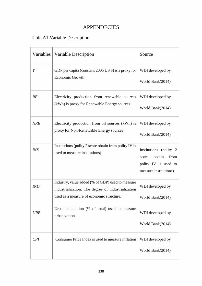
238
APPENDECIES
Table A1 Variable Description
Variables Variable Description Source
Y GDP per capita (constant 2005 US $) is a proxy for
Economic Growth
WDI developed by
World Bank(2014)
RE Electricity production from renewable sources
(kWh) is proxy for Renewable Energy sources
WDI developed by
World Bank(2014)
NRE Electricity production from oil sources (kWh) is
proxy for Non-Renewable Energy sources
WDI developed by
World Bank(2014)
INS Institutions (polity 2 score obtain from polity IV is
used to measure institutions) Institutions (polity 2
score obtain from
polity IV is used to
measure institutions)
IND Industry, value added (% of GDP) used to measure
industrialization. The degree of industrialization
used as a measure of economic structure.
WDI developed by
World Bank(2014)
URB Urban population (% of total) used to measure
urbanization WDI developed by
World Bank(2014)
CPI Consumer Price Index is used to measure inflation
WDI developed by
World Bank(2014)
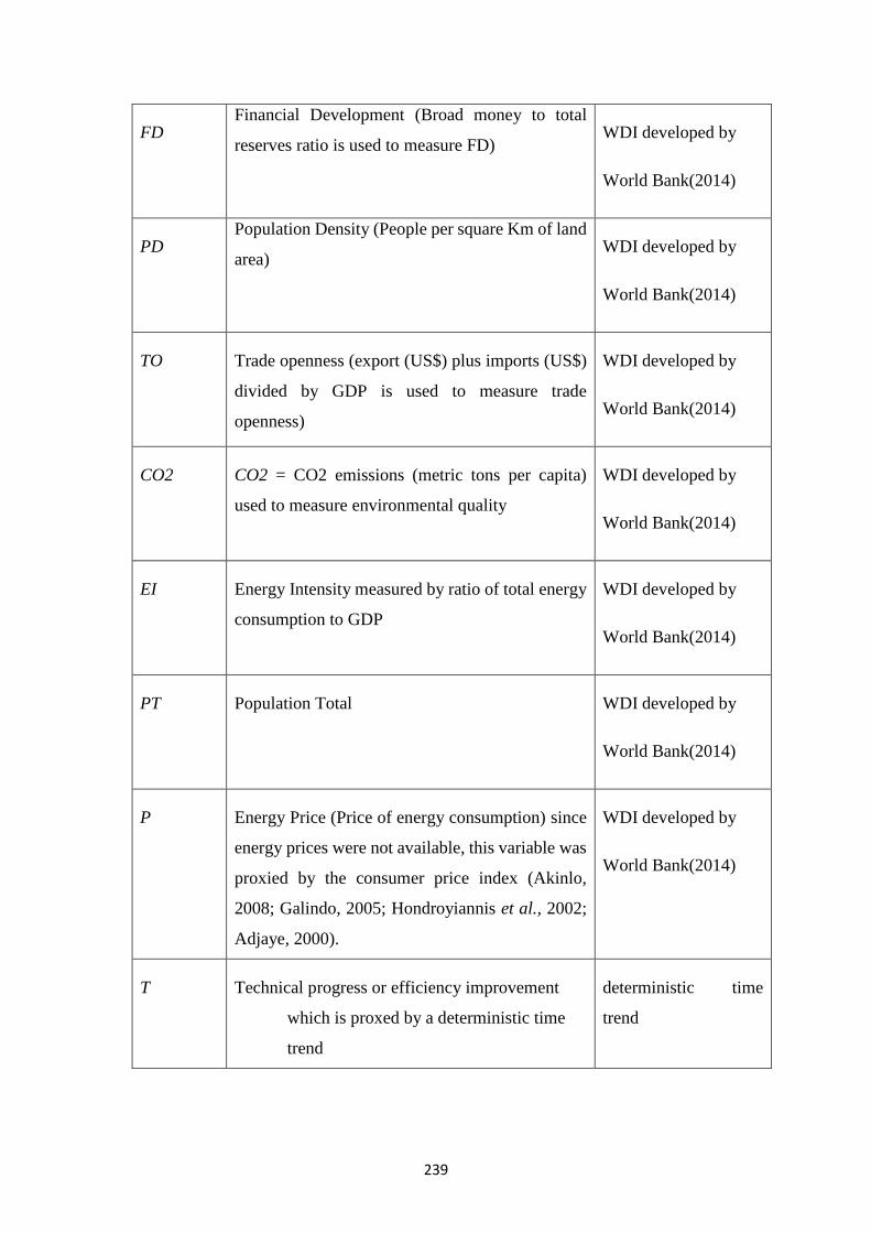
239
FD Financial Development (Broad money to total
reserves ratio is used to measure FD) WDI developed by
World Bank(2014)
PD Population Density (People per square Km of land
area) WDI developed by
World Bank(2014)
TO Trade openness (export (US$) plus imports (US$)
divided by GDP is used to measure trade
openness)
WDI developed by
World Bank(2014)
CO2 CO2 = CO2 emissions (metric tons per capita)
used to measure environmental quality
WDI developed by
World Bank(2014)
EI Energy Intensity measured by ratio of total energy
consumption to GDP
WDI developed by
World Bank(2014)
PT Population Total WDI developed by
World Bank(2014)
P Energy Price (Price of energy consumption) since
energy prices were not available, this variable was
proxied by the consumer price index (Akinlo,
2008; Galindo, 2005; Hondroyiannis et al., 2002;
Adjaye, 2000).
WDI developed by
World Bank(2014)
T Technical progress or efficiency improvement
which is proxed by a deterministic time
trend
deterministic time
trend
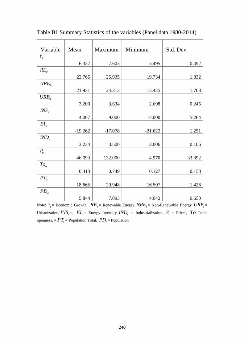
240
Table B1 Summary Statistics of the variables (Panel data 1980-2014)
Variable Mean
Maximum Minimum Std. Dev.
itY
6.327 7.603 5.495 0.492
itRE
22.765 25.935 19.734 1.832
itNRE
21.931 24.313 15.425 1.768
itURB
3.200 3.634 2.698 0.245
itINS
4.007 9.000 -7.000 5.264
itEI
-19.262 -17.078 -21.622 1.251
itIND
3.234 3.500 3.006 0.106
itP
46.093 132.000 4.570 33.392
itTo
0.413 0.749 0.127 0.158
itPT
18.665 20.948 16.507 1.426
itPD
5.844 7.093 4.642 0.650
Note: tY = Economic Growth, tRE = Renewable Energy, tNRE = Non-Renewable Energy tURB =
Urbanization, tINS =, tEI = Energy Intensity, tIND = Industrialization, tP = Prices, tTo Trade
openness, = tPT = Population Total, tPD = Population
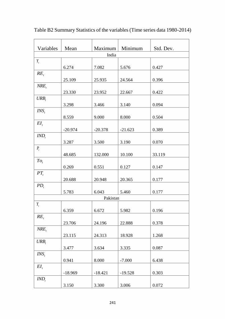
241
Table B2 Summary Statistics of the variables (Time series data 1980-2014)
Variables Mean
Maximum Minimum Std. Dev.
India
tY
6.274 7.082 5.676 0.427
tRE
25.109 25.935 24.564 0.396
tNRE
23.330 23.952 22.667 0.422
tURB
3.298 3.466 3.140 0.094
tINS
8.559 9.000 8.000 0.504
tEI
-20.974 -20.378 -21.623 0.389
tIND
3.287 3.500 3.190 0.070
tP
48.685 132.000 10.100 33.119
tTo
0.269 0.551 0.127 0.147
tPT
20.688 20.948 20.365 0.177
tPD
5.783 6.043 5.460 0.177
Pakistan
tY
6.359 6.672 5.982 0.196
tRE
23.706 24.196 22.888 0.378
tNRE
23.115 24.313 18.928 1.268
tURB
3.477 3.634 3.335 0.087
tINS
0.941 8.000 -7.000 6.438
tEI
-18.969 -18.421 -19.528 0.303
tIND
3.150 3.300 3.006 0.072
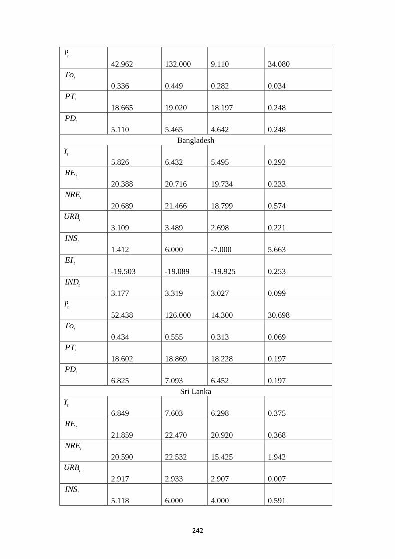
242
tP
42.962 132.000 9.110 34.080
tTo
0.336 0.449 0.282 0.034
tPT
18.665 19.020 18.197 0.248
tPD
5.110 5.465 4.642 0.248
Bangladesh
tY
5.826 6.432 5.495 0.292
tRE
20.388 20.716 19.734 0.233
tNRE
20.689 21.466 18.799 0.574
tURB
3.109 3.489 2.698 0.221
tINS
1.412 6.000 -7.000 5.663
tEI
-19.503 -19.089 -19.925 0.253
tIND
3.177 3.319 3.027 0.099
tP
52.438 126.000 14.300 30.698
tTo
0.434 0.555 0.313 0.069
tPT
18.602 18.869 18.228 0.197
tPD
6.825 7.093 6.452 0.197
Sri Lanka
tY
6.849 7.603 6.298 0.375
tRE
21.859 22.470 20.920 0.368
tNRE
20.590 22.532 15.425 1.942
tURB
2.917 2.933 2.907 0.007
tINS
5.118 6.000 4.000 0.591
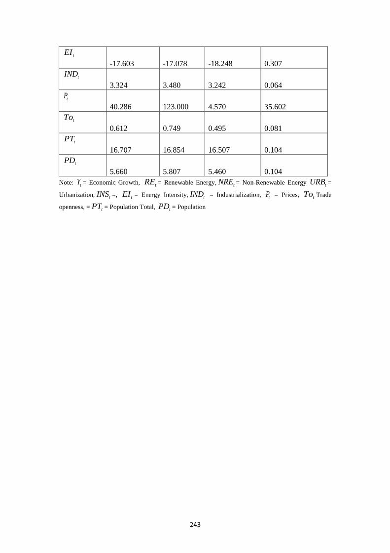
243
tEI
-17.603 -17.078 -18.248 0.307
tIND
3.324 3.480 3.242 0.064
tP
40.286 123.000 4.570 35.602
tTo
0.612 0.749 0.495 0.081
tPT
16.707 16.854 16.507 0.104
tPD
5.660 5.807 5.460 0.104
Note: tY = Economic Growth, tRE = Renewable Energy, tNRE = Non-Renewable Energy tURB =
Urbanization, tINS =, tEI = Energy Intensity, tIND = Industrialization, tP = Prices, tTo Trade
openness, = tPT = Population Total, tPD = Population
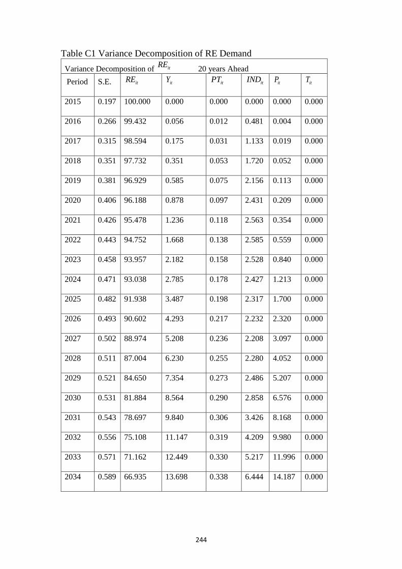
244
Table C1 Variance Decomposition of RE Demand
Variance Decomposition of itRE 20 years Ahead
Period S.E. itRE itY
itPT itIND
itP itT
2015 0.197 100.000 0.000 0.000 0.000 0.000 0.000
2016 0.266 99.432 0.056 0.012 0.481 0.004 0.000
2017 0.315 98.594 0.175 0.031 1.133 0.019 0.000
2018 0.351 97.732 0.351 0.053 1.720 0.052 0.000
2019 0.381 96.929 0.585 0.075 2.156 0.113 0.000
2020 0.406 96.188 0.878 0.097 2.431 0.209 0.000
2021 0.426 95.478 1.236 0.118 2.563 0.354 0.000
2022 0.443 94.752 1.668 0.138 2.585 0.559 0.000
2023 0.458 93.957 2.182 0.158 2.528 0.840 0.000
2024 0.471 93.038 2.785 0.178 2.427 1.213 0.000
2025 0.482 91.938 3.487 0.198 2.317 1.700 0.000
2026 0.493 90.602 4.293 0.217 2.232 2.320 0.000
2027 0.502 88.974 5.208 0.236 2.208 3.097 0.000
2028 0.511 87.004 6.230 0.255 2.280 4.052 0.000
2029 0.521 84.650 7.354 0.273 2.486 5.207 0.000
2030 0.531 81.884 8.564 0.290 2.858 6.576 0.000
2031 0.543 78.697 9.840 0.306 3.426 8.168 0.000
2032 0.556 75.108 11.147 0.319 4.209 9.980 0.000
2033 0.571 71.162 12.449 0.330 5.217 11.996 0.000
2034 0.589 66.935 13.698 0.338 6.444 14.187 0.000
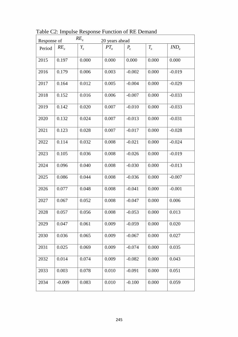
245
Table C2: Impulse Response Function of RE Demand
Response of itRE 20 years ahead
Period itRE itY
itPT itP
itT itIND
2015 0.197 0.000 0.000 0.000 0.000 0.000
2016 0.179 0.006 0.003 -0.002 0.000 -0.019
2017 0.164 0.012 0.005 -0.004 0.000 -0.029
2018 0.152 0.016 0.006 -0.007 0.000 -0.033
2019 0.142 0.020 0.007 -0.010 0.000 -0.033
2020 0.132 0.024 0.007 -0.013 0.000 -0.031
2021 0.123 0.028 0.007 -0.017 0.000 -0.028
2022 0.114 0.032 0.008 -0.021 0.000 -0.024
2023 0.105 0.036 0.008 -0.026 0.000 -0.019
2024 0.096 0.040 0.008 -0.030 0.000 -0.013
2025 0.086 0.044 0.008 -0.036 0.000 -0.007
2026 0.077 0.048 0.008 -0.041 0.000 -0.001
2027 0.067 0.052 0.008 -0.047 0.000 0.006
2028 0.057 0.056 0.008 -0.053 0.000 0.013
2029 0.047 0.061 0.009 -0.059 0.000 0.020
2030 0.036 0.065 0.009 -0.067 0.000 0.027
2031 0.025 0.069 0.009 -0.074 0.000 0.035
2032 0.014 0.074 0.009 -0.082 0.000 0.043
2033 0.003 0.078 0.010 -0.091 0.000 0.051
2034 -0.009 0.083 0.010 -0.100 0.000 0.059
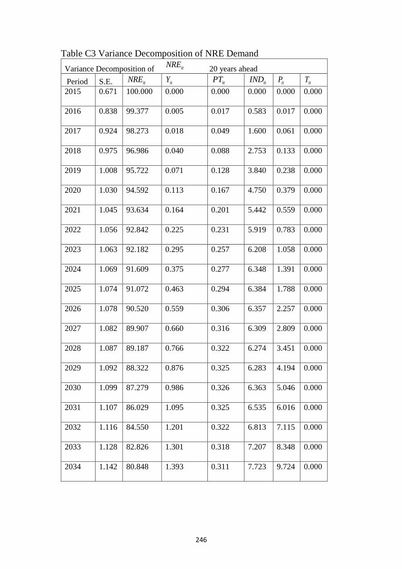
246
Table C3 Variance Decomposition of NRE Demand
Variance Decomposition of itNRE 20 years ahead
Period S.E. itNRE itY
itPT itIND
itP itT
2015 0.671 100.000 0.000 0.000 0.000 0.000 0.000
2016 0.838 99.377 0.005 0.017 0.583 0.017 0.000
2017 0.924 98.273 0.018 0.049 1.600 0.061 0.000
2018 0.975 96.986 0.040 0.088 2.753 0.133 0.000
2019 1.008 95.722 0.071 0.128 3.840 0.238 0.000
2020 1.030 94.592 0.113 0.167 4.750 0.379 0.000
2021 1.045 93.634 0.164 0.201 5.442 0.559 0.000
2022 1.056 92.842 0.225 0.231 5.919 0.783 0.000
2023 1.063 92.182 0.295 0.257 6.208 1.058 0.000
2024 1.069 91.609 0.375 0.277 6.348 1.391 0.000
2025 1.074 91.072 0.463 0.294 6.384 1.788 0.000
2026 1.078 90.520 0.559 0.306 6.357 2.257 0.000
2027 1.082 89.907 0.660 0.316 6.309 2.809 0.000
2028 1.087 89.187 0.766 0.322 6.274 3.451 0.000
2029 1.092 88.322 0.876 0.325 6.283 4.194 0.000
2030 1.099 87.279 0.986 0.326 6.363 5.046 0.000
2031 1.107 86.029 1.095 0.325 6.535 6.016 0.000
2032 1.116 84.550 1.201 0.322 6.813 7.115 0.000
2033 1.128 82.826 1.301 0.318 7.207 8.348 0.000
2034 1.142 80.848 1.393 0.311 7.723 9.724 0.000
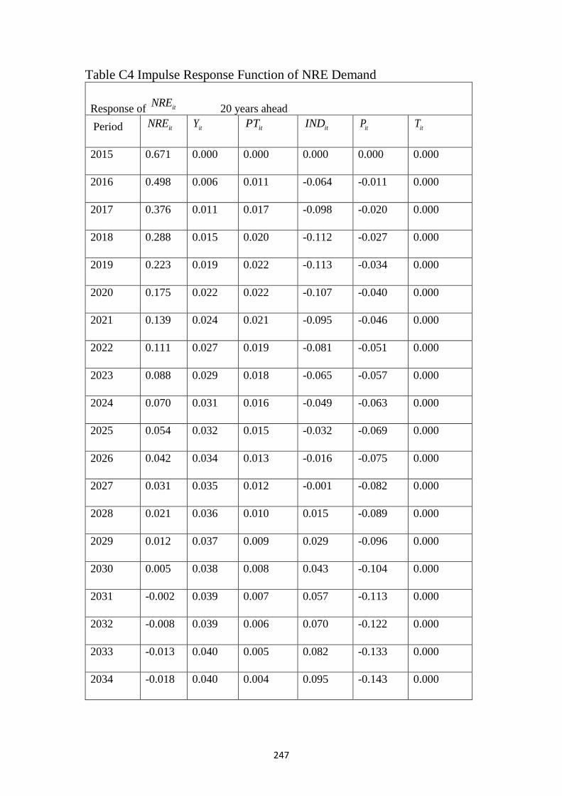
247
Table C4 Impulse Response Function of NRE Demand
Response of itNRE 20 years ahead
Period itNRE itY
itPT itIND
itP itT
2015 0.671 0.000 0.000 0.000 0.000 0.000
2016 0.498 0.006 0.011 -0.064 -0.011 0.000
2017 0.376 0.011 0.017 -0.098 -0.020 0.000
2018 0.288 0.015 0.020 -0.112 -0.027 0.000
2019 0.223 0.019 0.022 -0.113 -0.034 0.000
2020 0.175 0.022 0.022 -0.107 -0.040 0.000
2021 0.139 0.024 0.021 -0.095 -0.046 0.000
2022 0.111 0.027 0.019 -0.081 -0.051 0.000
2023 0.088 0.029 0.018 -0.065 -0.057 0.000
2024 0.070 0.031 0.016 -0.049 -0.063 0.000
2025 0.054 0.032 0.015 -0.032 -0.069 0.000
2026 0.042 0.034 0.013 -0.016 -0.075 0.000
2027 0.031 0.035 0.012 -0.001 -0.082 0.000
2028 0.021 0.036 0.010 0.015 -0.089 0.000
2029 0.012 0.037 0.009 0.029 -0.096 0.000
2030 0.005 0.038 0.008 0.043 -0.104 0.000
2031 -0.002 0.039 0.007 0.057 -0.113 0.000
2032 -0.008 0.039 0.006 0.070 -0.122 0.000
2033 -0.013 0.040 0.005 0.082 -0.133 0.000
2034 -0.018 0.040 0.004 0.095 -0.143 0.000
Top Related