


Languages
Pages
Legal

Principle Component Analysis
and
Model Reduction for Dynamical Systems
D.C. Sorensen
Virginia Tech 12 Nov 2004

Protein Substate Modeling and Identification
PCA Dimension Reduction Using the SVD• Tod Romo • George Phillips
T.D. Romo, J.B. Clarage, D.C. Sorensen and G.N. Phillips, Jr., Automatic Identification of
Discrete Substates in Proteins: Singular Value Decomposition Analysis of Time Averaged
Crystallographic Refinements, Proteins: Structure, Function, and Genetics22,311-321,(1995).
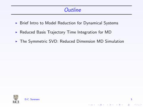
Outline
I Brief Intro to Model Reduction for Dynamical Systems
I Reduced Basis Trajectory Time Integration for MD
I The Symmetric SVD: Reduced Dimension MD Simulation
D.C. Sorensen 3
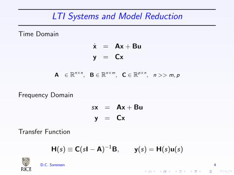
LTI Systems and Model Reduction
Time Domain
x = Ax + Bu
y = Cx
A ∈ Rn×n, B ∈ Rn×m, C ∈ Rp×n, n >> m, p
Frequency Domain
sx = Ax + Bu
y = Cx
Transfer Function
H(s) ≡ C(sI− A)−1B, y(s) = H(s)u(s)
D.C. Sorensen 4

Model Reduction
Construct a new system {A, B, C} with LOW dimension k << n
˙x = Ax + Bu
y = Cx
Goal: Preserve system response
y should approximate y
Projection: x(t) = V ˆx(t) and V ˙x = AVx + Bu
D.C. Sorensen 5
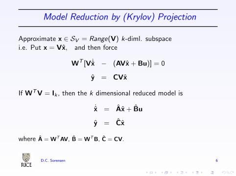
Model Reduction by (Krylov) Projection
Approximate x ∈ SV = Range(V) k-diml. subspacei.e. Put x = Vx, and then force
WT [V ˙x − (AVx + Bu)] = 0
y = CVx
If WTV = Ik , then the k dimensional reduced model is
˙x = Ax + Bu
y = Cx
where A = WTAV, B = WTB, C = CV.
D.C. Sorensen 6
Moment Matching ↔ Krylov Subspace Projection
Pade via Lanczos (PVL)
Freund, Feldmann
Bai
Multipoint Rational Interpolation
Grimme
Gallivan, Grimme, Van Dooren
Gugercin, Antoulas, Beattie
D.C. Sorensen 7
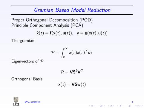
Gramian Based Model Reduction
Proper Orthogonal Decomposition (POD)Principle Component Analysis (PCA)
x(t) = f(x(t),u(t)), y = g(x(t),u(t))
The gramian
P =
∫ ∞
ox(τ)x(τ)Tdτ
Eigenvectors of P
P = VS2VT
Orthogonal Basisx(t) = VSw(t)
D.C. Sorensen 8
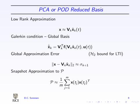
PCA or POD Reduced Basis
Low Rank Approximation
x ≈ Vk xk(t)
Galerkin condition – Global Basis
˙xk = VTk f(Vk xk(t),u(t))
Global Approximation Error (H2 bound for LTI)
‖x− Vk xk‖2 ≈ σk+1
Snapshot Approximation to P
P ≈ 1
m
m∑j=1
x(tj)x(tj)T
D.C. Sorensen 9
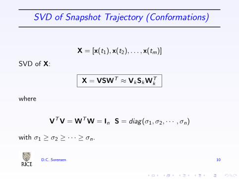
SVD of Snapshot Trajectory (Conformations)
X = [x(t1), x(t2), . . . , x(tm)]
SVD of X:
X = VSWT ≈ VkSkWTk
where
VTV = WTW = In S = diag(σ1, σ2, · · · , σn)
with σ1 ≥ σ2 ≥ · · · ≥ σn.
D.C. Sorensen 10
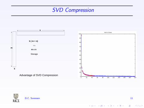
SVD Compression
m
k ( m + n)
m x n
v.s.
Storage
Advantage of SVD Compression
k
n
0 20 40 60 80 100 120 140 160 180 2000
10
20
30
40
50
60
70
80
90
100SVD of Clown
D.C. Sorensen 11
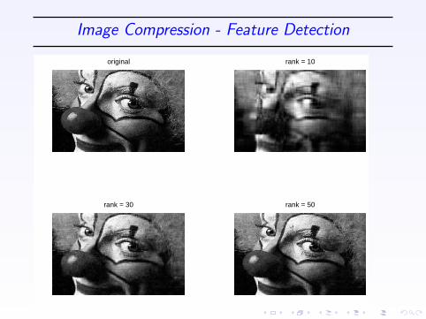
Image Compression - Feature Detection
original rank = 10
rank = 30 rank = 50
POD in CFD
Extensive Literature
Karhunen-Loeve, L. Sirovich
Burns, King
Kunisch and Volkwein
Many, many others
Incorporating Observations – Balancing
Lall, Marsden and Glavaski
K. Willcox and J. Peraire
D.C. Sorensen 13
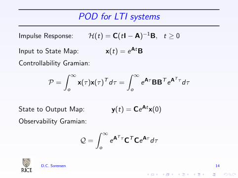
POD for LTI systems
Impulse Response: H(t) = C(tI− A)−1B, t ≥ 0
Input to State Map: x(t) = eAtB
Controllability Gramian:
P =
∫ ∞
ox(τ)x(τ)Tdτ =
∫ ∞
oeAτBBT eAT τdτ
State to Output Map: y(t) = CeAtx(0)
Observability Gramian:
Q =
∫ ∞
oeAT τCTCeAτdτ
D.C. Sorensen 14

Balanced Reduction (Moore 81)
Lyapunov Equations for system Gramians
AP + PAT
+ BBT
= 0 ATQ+QA + C
TC = 0
With P = Q = S : Want Gramians Diagonal and Equal
States Difficult to Reach are also Difficult to Observe
Reduced Model Ak = WTk AVk , Bk = WT
k B , Ck = CkVk
I PVk = WkSk QWk = VkSk
I Reduced Model Gramians Pk = Sk and Qk = Sk .
D.C. Sorensen 15
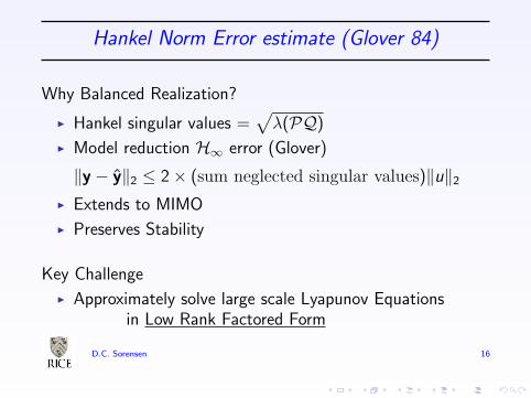
Hankel Norm Error estimate (Glover 84)
Why Balanced Realization?
I Hankel singular values =√
λ(PQ)
I Model reduction H∞ error (Glover)
‖y − y‖2 ≤ 2× (sum neglected singular values)‖u‖2I Extends to MIMO
I Preserves Stability
Key Challenge
I Approximately solve large scale Lyapunov Equationsin Low Rank Factored Form
D.C. Sorensen 16
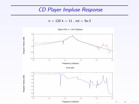
CD Player Impluse Response
n = 120 k = 11 , tol = 5e-3
Frequency (rad/sec)
Sin
gula
r V
alue
s (d
B)
Sigma Plot: n = 120 CDplayer
100
101
102
103
104
105
−150
−100
−50
0
50
Frequency (rad/sec)
Sin
gula
r V
alue
s (d
B)
Error plot
100
101
102
103
104
105
−90
−80
−70
−60
−50
−40
−30
−20
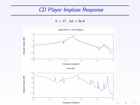
CD Player Impluse Response
k = 17 , tol = 5e-4
Frequency (rad/sec)
Sin
gula
r V
alue
s (d
B)
Sigma Plot: n = 120 CDplayer
100
101
102
103
104
105
−150
−100
−50
0
50
Frequency (rad/sec)
Sin
gula
r V
alue
s (d
B)
Error plot
100
101
102
103
104
105
−80
−70
−60
−50
−40
−30

CD Player Impluse Response
k = 31 , tol = 5e-5
Frequency (rad/sec)
Sin
gula
r V
alue
s (d
B)
Sigma Plot: n = 120 CDplayer
100
101
102
103
104
105
−150
−100
−50
0
50
Frequency (rad/sec)
Sin
gula
r V
alue
s (d
B)
Error plot
100
101
102
103
104
105
−100
−90
−80
−70
−60
−50
−40

CD Player - Hankel Singular Values
0 20 40 60 80 100 12010
−14
10−12
10−10
10−8
10−6
10−4
10−2
100
102
Hankel Singular Values
D.C. Sorensen 20
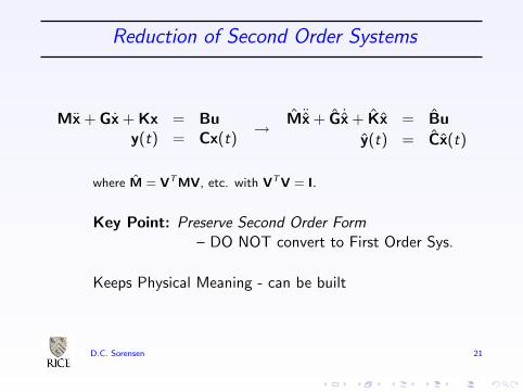
Reduction of Second Order Systems
Mx + Gx + Kx = Buy(t) = Cx(t)
→ M¨x + G ˙x + Kx = Bu
y(t) = Cx(t)
where M = VTMV, etc. with VTV = I.
Key Point: Preserve Second Order Form– DO NOT convert to First Order Sys.
Keeps Physical Meaning - can be built
D.C. Sorensen 21
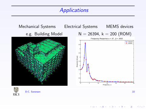
Applications
Mechanical Systems Electrical Systems MEMS devices
e.g. Building Model N = 26394, k = 200 (ROM)
0 5 10 15 20 25 300
0.5
1
1.5
2
2.5
3
3.5
4
4.5
5Frequency Response α = .67 , β = .0032
Frequency ω
Res
pons
e |G
( jω
)|
reducedoriginal
D.C. Sorensen 22
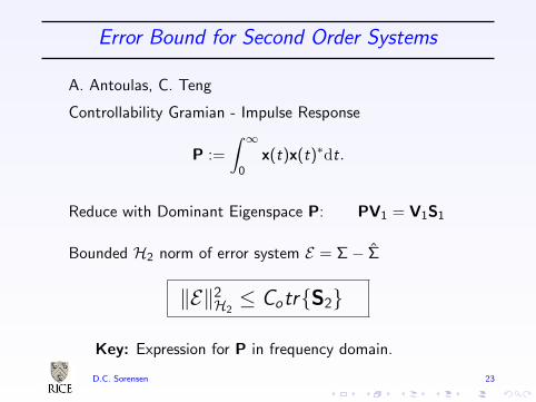
Error Bound for Second Order Systems
A. Antoulas, C. Teng
Controllability Gramian - Impulse Response
P :=
∫ ∞
0x(t)x(t)∗dt.
Reduce with Dominant Eigenspace P: PV1 = V1S1
Bounded H2 norm of error system E = Σ− Σ
‖E‖2H2≤ Cotr{S2}
Key: Expression for P in frequency domain.
D.C. Sorensen 23

PCA Model Reduction for Molecular Dynamics
• Rachel Vincent • Monte Pettitt
D.C. Sorensen 24
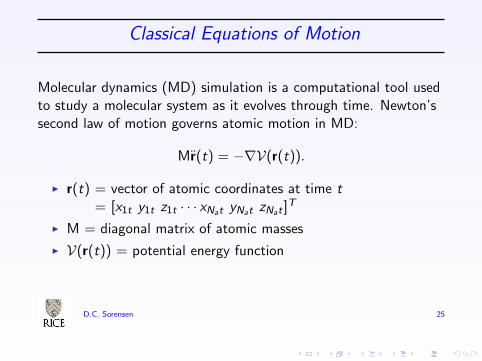
Classical Equations of Motion
Molecular dynamics (MD) simulation is a computational tool usedto study a molecular system as it evolves through time. Newton’ssecond law of motion governs atomic motion in MD:
Mr(t) = −∇V(r(t)).
I r(t) = vector of atomic coordinates at time t= [x1t y1t z1t · · · xNat yNat zNat ]
T
I M = diagonal matrix of atomic masses
I V(r(t)) = potential energy function
D.C. Sorensen 25
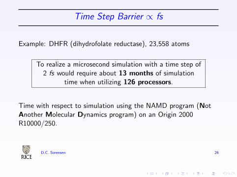
Time Step Barrier ∝ fs
Example: DHFR (dihydrofolate reductase), 23,558 atoms
To realize a microsecond simulation with a time step of2 fs would require about 13 months of simulation
time when utilizing 126 processors.
Time with respect to simulation using the NAMD program (NotAnother Molecular Dynamics program) on an Origin 2000R10000/250.
D.C. Sorensen 26
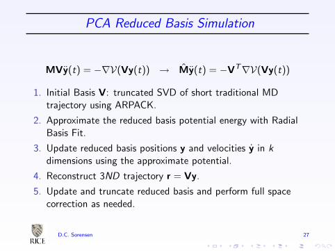
PCA Reduced Basis Simulation
MVy(t) = −∇V(Vy(t)) → My(t) = −VT∇V(Vy(t))
1. Initial Basis V: truncated SVD of short traditional MDtrajectory using ARPACK.
2. Approximate the reduced basis potential energy with RadialBasis Fit.
3. Update reduced basis positions y and velocities y in kdimensions using the approximate potential.
4. Reconstruct 3ND trajectory r = Vy.
5. Update and truncate reduced basis and perform full spacecorrection as needed.
D.C. Sorensen 27
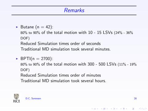
Remarks
I Butane (n = 42):80% to 90% of the total motion with 10 - 15 LSVs (24% - 36%
DOF)
Reduced Simulation times order of secondsTraditional MD simulation took several minutes.
I BPTI(n = 2700):80% to 90% of the total motion with 300 - 500 LSVs (11% - 19%
DOF)
Reduced Simulation times order of minutesTraditional MD simulation took several hours.
D.C. Sorensen 28
Symmetry Preserving SVD (Mili Shah)
Collaboration with the Physical and Biological Computing Group
I Lydia Kavraki
I Mark Moll
I David Schwarz
I Amarda Shehua
I Allison Heath
D.C. Sorensen 29

Symmetry in HIV-1 protease
Backbone representation of HIV-1 protease (from M. Moll)
bound to an inhibitor (shown in orange)Uses PCA dimension reduction of Molecular Dynamics Simulations
Symmetry across a plane should be present
D.C. Sorensen 30
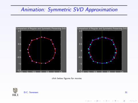
Animation: Symmetric SVD Approximation
−1.5 −1 −0.5 0 0.5 1 1.5−1.5
−1
−0.5
0
0.5
1
1.5Comparison of Regular and Symmetric Preserving SVD
−1.5 −1 −0.5 0 0.5 1 1.5−1.5
−1
−0.5
0
0.5
1
1.5Comparison of Regular and Symmetric Preserving SVD
click below figures for movies
D.C. Sorensen 31
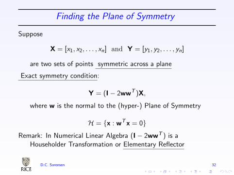
Finding the Plane of Symmetry
Suppose
X = [x1, x2, . . . , xn] and Y = [y1, y2, . . . , yn]
are two sets of points symmetric across a plane
Exact symmetry condition:
Y = (I− 2wwT )X,
where w is the normal to the (hyper-) Plane of Symmetry
H = {x : wTx = 0}
Remark: In Numerical Linear Algebra (I− 2wwT ) is aHouseholder Transformation or Elementary Reflector
D.C. Sorensen 32
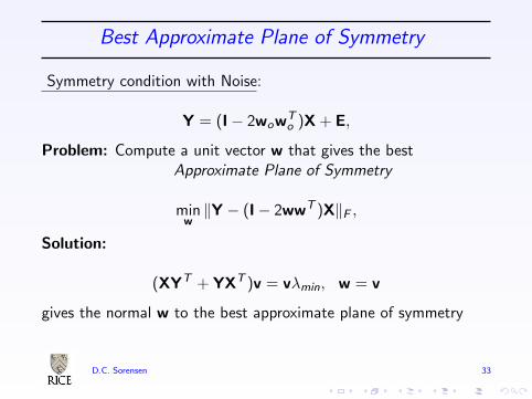
Best Approximate Plane of Symmetry
Symmetry condition with Noise:
Y = (I− 2wowTo )X + E,
Problem: Compute a unit vector w that gives the bestApproximate Plane of Symmetry
minw‖Y − (I− 2wwT )X‖F ,
Solution:
(XYT + YXT )v = vλmin, w = v
gives the normal w to the best approximate plane of symmetry
D.C. Sorensen 33
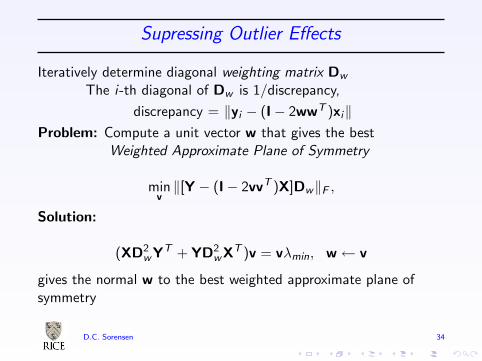
Supressing Outlier Effects
Iteratively determine diagonal weighting matrix Dw
The i-th diagonal of Dw is 1/discrepancy,
discrepancy = ‖yi − (I− 2wwT )xi‖Problem: Compute a unit vector w that gives the best
Weighted Approximate Plane of Symmetry
minv‖[Y − (I− 2vvT )X]Dw‖F ,
Solution:
(XD2wYT + YD2
wXT )v = vλmin, w← v
gives the normal w to the best weighted approximate plane ofsymmetry
D.C. Sorensen 34
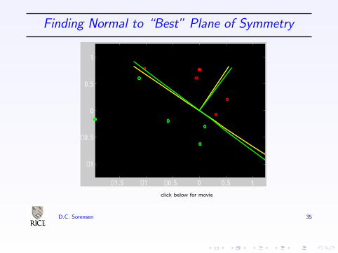
Finding Normal to “Best” Plane of Symmetry
−1.5 −1 −0.5 0 0.5 1
−1
−0.5
0
0.5
1
click below for movie
D.C. Sorensen 35
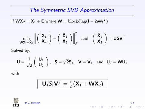
The Symmetric SVD Approximation
If WX2 = X1 + E where W = blockdiag(I− 2wwT )
minWX2=X1
∥∥∥∥(X1
X2
)−
(X1
X2
)∥∥∥∥2
F
and(
X1
X2
)= USVT
Solved by:
U =1√2
(U1
U2
), S =
√2S1, V = V1. and U2 = WU1,
with
U1S1VT1 = 1
2 (X1 + WX2)
D.C. Sorensen 36

Symmetric Major Modes: HIV-1 protease
I Major mode regular SVD is red
I Major mode SYMMETRIC SVD is blue
I 3120 atoms (3*3120=9360 degrees of freedom)
I MD trajectory consisted of 10000 conformations (NAMD)
I SVD and SymSVD used P ARPACK on a Linux cluster
I dual-processor nodes; 1600MHz AMD Athlon processors, 1GBRAM per node. 1GB/s Ethernet connection . 12 Processors= 6 nodes.
I First 10 standard singular vectors: 88 secs.
I First 10 symmetric singular vectors: 131 secs.
D.C. Sorensen 37
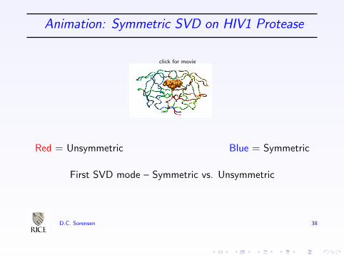
Animation: Symmetric SVD on HIV1 Protease
click for movie
Red = Unsymmetric Blue = Symmetric
First SVD mode – Symmetric vs. Unsymmetric
D.C. Sorensen 38
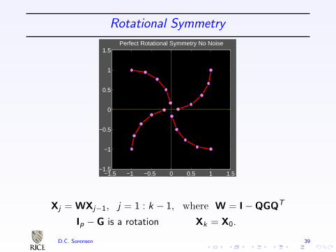
Rotational Symmetry
−1.5 −1 −0.5 0 0.5 1 1.5−1.5
−1
−0.5
0
0.5
1
1.5Perfect Rotational Symmetry No Noise
Xj = WXj−1, j = 1 : k − 1, where W = I−QGQT
Ip − G is a rotation Xk = X0.
D.C. Sorensen 39
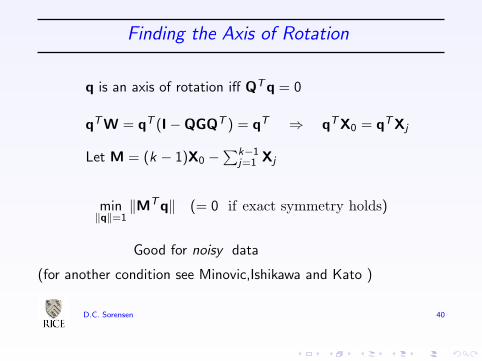
Finding the Axis of Rotation
q is an axis of rotation iff QTq = 0
qTW = qT (I−QGQT ) = qT ⇒ qTX0 = qTXj
Let M = (k − 1)X0 −∑k−1
j=1 Xj
min‖q‖=1
‖MTq‖ (= 0 if exact symmetry holds)
Good for noisy data
(for another condition see Minovic,Ishikawa and Kato )
D.C. Sorensen 40
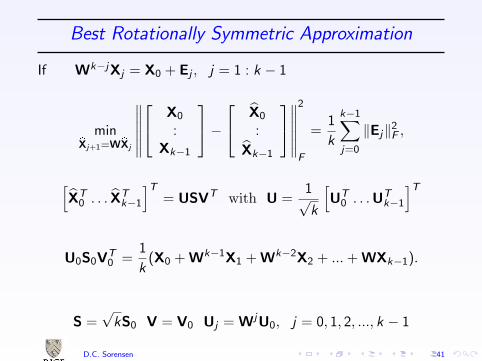
Best Rotationally Symmetric Approximation
If Wk−jXj = X0 + Ej , j = 1 : k − 1
minbXj+1=WbXj
∥∥∥∥∥∥ X0
:Xk−1
− X0
:
Xk−1
∥∥∥∥∥∥2
F
=1
k
k−1∑j=0
‖Ej‖2F ,
[XT
0 . . . XTk−1
]T= USVT with U =
1√k
[UT
0 . . .UTk−1
]T
U0S0VT0 =
1
k(X0 + Wk−1X1 + Wk−2X2 + ... + WXk−1).
S =√
kS0 V = V0 Uj = WjU0, j = 0, 1, 2, ..., k − 1
D.C. Sorensen 41
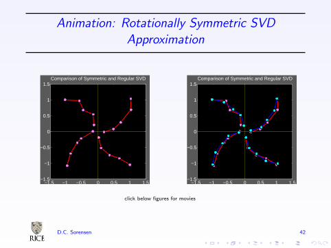
Animation: Rotationally Symmetric SVDApproximation
−1.5 −1 −0.5 0 0.5 1 1.5−1.5
−1
−0.5
0
0.5
1
1.5Comparison of Symmetric and Regular SVD
−1.5 −1 −0.5 0 0.5 1 1.5−1.5
−1
−0.5
0
0.5
1
1.5Comparison of Symmetric and Regular SVD
click below figures for movies
D.C. Sorensen 42

Animation: Rotationally Symmetric SVD on HIV1
click for movie
Red = Unsymmetric Blue = Symmetric
Second SVD mode – Rotationally Symmetric vs. Unsymmetric
D.C. Sorensen 43

Potential for Symmetric SVD
I Obtain a Symmetric PCA reduced dimension approximatetrajectory
I Test Hypothesis of Symmetry in an Unknown Protein
I Locate Symmeteric Sub-Structures
Things to Do:
I Improve convergence rate for finding w
I Give a complete analysis of convergence
I Give a complete analysis of discrepancy weighting
I Extend to more complex symmetries
I Find New Applications
D.C. Sorensen 44
Contact Info.
e-mail: [email protected]
web page: www.caam.rice.edu/ ˜ sorensen/
ARPACK: www.caam.rice.edu/software/ARPACK/
Top Related