Population Aging and International Capital Flows

David Domeij and Martin Flodén1

Department of Economics, Stockholm School of EconomicsDepartment of Economics, Stockholm School of Economics and CEPR

March 14, 2005

Abstract

We use the neoclassical growth framework to model international capital flowsin a world with exogenous demographic change. We compare model implica-tions and actual current account data and find that the model explains a smallbut significant fraction of capital flows between OECD countries, in particularafter 1985.

JEL classification: E22; F21; F41; F47

Keywords: current account; international capital mobility; demographics; Feldstein-Horioka puzzle

1We thank seminar participants at the Stockholm School of Economics, CERGE-EI, London School ofEconomics, Bocconi University, European University Institute, ESSIM 2004, and SED 2004 for comments.We also thank the Wallander and Hedelius Foundation and the Bank of Sweden Tercentenary Foundationfor generous funding.

1 Introduction

According to the life-cycle theory, consumption as a fraction of income varies with age.

Taking this argument one step further, a country’s saving rate depends on the age-structure

of its population. This direct link between demographics and savings, investments, and

capital flows has been addressed in a number of papers. Fair and Dominguez (1991) find

mixed evidence for this story using quarterly U.S. data, while Higgins and Williamson

(1997), Higgins (1998), and Lane and Milesi-Ferretti (2001) find strong support for the

story using lower-frequency data for a large number of countries.

In this paper, we use another approach to examine the same link from demographics

to savings, investment, and international capital flows. Rather than directly testing for

correlations between a country’s age-structure and these macroeconomic variables, we use

a standard neoclassical model that is consistent with the life-cycle theory. We calibrate

this model with population data and projections for a large number of countries, and

examine if the data generated by the model can explain real-world capital flows.

In addition to controlling for the domestic age-distribution this approach allows us to

control for a changing demographic structure in the world economy. In the coming decades,

most developed countries will face aging populations and smaller fractions of prime-age

workers in the population. Theory and the empirical results found by for example Higgins

(1998) then predict that current account balances will fall. It is not possible, however,

that all countries simultaneously run current account deficits. The correlations between

age-structure and capital flows will then not be robust.2 We get around this problem by

using a general equilibrium model, where we force the sum of current accounts in the world

economy to balance in each period.

Many studies (see the survey below) have used calibrated models similar to ours to examine

the consequences of population aging. These studies have typically not tested the model’s

ability to explain historical data. Our paper therefore also contributes by providing a test

2Higgins (1998) was well aware of this problem. For example, he argued that "out-of-sample projectionscannot capture the general equilibrium effects of a novel pattern of global demographic change" (p. 366).

1

of the standard model used frequently in the literature.

We find that the model generates data that can explain a small but significant fraction

of real-world capital flows between countries. This finding both reinforces the results

in previous empirical studies documenting a correlation between age-distributions and

capital flows, and supports the use of calibrated life-cycle models to study the effects of

demographic change.

The model performs better when we restrict attention to data from 1985 and onwards.

This result is consistent with the low mobility of capital documented by Feldstein and

Horioka (1980), and Blanchard and Giavazzi’s (2002) finding that capital has become

more mobile in the last two decades.

As already mentioned, a number of studies use calibrated life-cycle models to examine

how population aging will affect saving and capital flows. Much of this work either treat

economies as closed (following Auerbach and Kotlikoff 1987), or as small open economies

facing exogenous and constant factor prices (following Auerbach et al. 1989). Exceptions

exist, though. Cutler et al. (1990) use a two-region model for the United States and the

non-U.S. OECD countries and find that the U.S. demographic transition is affected by

capital inflows from the other OECD countries. They also point out that the population

aging process will be less dramatic in the United States than in most other OECD coun-

tries. When looking ahead from 1990, their model therefore predicted that the savings

rate in the United States would increase less than in the other countries, and consequently

that the United States would run current account deficits during the 1990’s.3

Brooks (2003) uses an overlapping generations model where individuals live for four peri-

ods, and solves for the equilibrium in a world economy with eight regions. He calibrates

the model with historical and projected population data to generate paths for capital flows

motivated by demographics. In work parallel to and independent of ours, Henriksen (2002)

3Other papers that solve for general equilibrium capital flows induced by demographic change are At-tanasio and Violante (2000), and Flodén (2003). Attanasio and Violante examine how the Latin Americandemographic transition would be affected by capital mobility, while Flodén examines future capital flowsbetween 15 OECD countries.

2

and Feroli (2003) build on Brooks but introduce a richer life-cycle structure. Henriksen

focuses on Japan and the United States while Feroli calibrates a four-region world con-

sisting of the United States, Japan, Germany, and other European countries. They both

find that their models predict American current account deficits and Japanese surpluses

during the last decades, as in the real-world data.

The paper is organized as follows. We present the model in Section 2. In Section 3 we

describe how we calibrate and solve the model. In Section 4 we compare capital flows

implied by the model with real-world data. Finally, in Section 5 we examine the model’s

implications for future capital flows.

2 The Model

We consider a model of a world economy. Each country is populated by overlapping

generations of households that solve a standard life-cycle consumption problem. The

demographic development is exogenous and the production technology is identical across

countries, except that we allow for permanent differences in factor productivity. We assume

that labor is immobile but that capital can move freely between countries.

2.1 The Household’s Optimization Problem

Households enter the labor market at age 20, raise an exogenous number of children

between ages 20 and 49, and die at age N or earlier. Survival between periods is stochastic

and there are domestic annuity markets for savings. Households maximize adult life-time

utility,

(1) max{cs,as+1}Ns=20,b

NXs=20

βsΦs(cs/ψs)

1−µ

1− µ+ΘβNbΦNb

b1−µ

1− µ

3

subject to

(2) cs + as+1 + bI (s = Nb) = ys +(1 + ras ) asφs−1,s

ys = (1− τ s)wshsI (s < 65) + dsI (s ≥ 65)

aN+1 ≥ 0

and

a20 given.

Here β is the discount factor, φs−1,s denotes the survival probability from period s− 1 toperiod s, and Φs = Φ19

Ys

σ=20φσ−1,σ is the unconditional probability that the household

is alive at age s. We normalize Φ19 = 1. Θ is a parameter determining the importance

of bequests, b, and Nb denotes the age at which bequests are given. Total household

consumption is denoted by c, and ψ is the number of consumption equivalents in the

household. Labor supply in efficiency units, h, is exogenous but depends on age. House-

holds hold assets, a, consisting of physical capital and shares in the representative firm in

each country as described below. Finally, I (·) is an indicator function, and ra, w, y, τ ,

and d denote the return on household assets, the wage rate, income, the social security

tax, and the pension benefit.4

2.2 The Pension System

In each country, the government runs a pay-as-you-go, defined-benefits pension system.

There is a flat pension tax on labor income, and the tax revenue is distributed as lump-

sum pension benefits among all retirees (aged 65 and above). The budget constraint for

the pension system in a country is thus

(3) τ t =dtPN

s=65 Pt,swtHt

4To simplify notation, subscripts s on prices r and w denote time relative to the household’s birth year,while subscripts t will be used to denote actual time.

4

where Pt,s denotes the number of people of age s at date t and H is the aggregate labor

supply in efficiency units.

2.3 Production and Asset Markets

The representative firm in a country rents labor H at the wage rate w, and capital K at

the world market price r to maximize the discounted value of dividends,

max{H,K}

∞Xt=1

ÃtY

τ=1

1

1 + raτ

!πt,

where

(4) πt = Kθt (ZtHt)

1−θ − (rt + δ)Kt − Ξ (Kt−1,Kt)− wtHt,

and Zt is productivity per efficiency unit of labor, δ is the depreciation rate of capital, K0

is given, and Ξ is the cost of changing the size of the capital stock used by the firm. We

assume that capital is not installed, so firms only incur adjustment costs if they change

the size of the capital stock used in production.5 There is therefore one world market for

physical capital, and capital and consumption goods are perfect substitutes.

The first order conditions to the firm’s problem are then

(5) wt = (1− θ)Kθt Z

1−θt H−θ

t

and

(6) θ (ZtHt/Kt)1−θ − (rt + δ)− Ξ2 (Kt−1,Kt)− Ξ1 (Kt,Kt+1)

1 + rat+1= 0

where subscripts on Ξ denote derivatives.

5The costs we have in mind are in particular associated with adjusting the size of the labor force.For example, the firm can rent a particular set of machinery and costlessly substitute this machinery foranother identical set in the next period. But if the firm rents more machinery, it will have to hire andtrain new workers.

5

Since there are adjustment costs, dividends may be non-zero and will accrue to the firm’s

owners. The households’ assets therefore include shares in the firms in addition to physical

capital. More specifically, for a household of age s in country i at time t, the portfolio is

ai,t,s = ki,t,s +Xj

Qj,tκj,i,t,s

where k denotes the household’s physical capital and κj denotes the household’s share in

the representative firm in country j, and Qj denotes the price of these shares. Note that

the value of the representative firm in country j at time t is

(7) Vj,t =Xi

NXs=20

Qj,tκj,i,t,s.

2.4 Equilibrium

Let R = {rt}∞1 and Ra = {rat }∞1 denote the paths for returns on physical capital and

household portfolios, and let Wi = {wi,t}∞t=1, Ki = {Ki,t}∞t=1, Qi = {Qi,t}∞t=1, Πi ={πi,t}∞t=1, Vi = {Vi,t}∞t=1, Ti = {τ i,t}∞t=1 , Di = {di,t}∞t=1, denote the paths for wages,capital, share prices, dividends, firm values, social security taxes, and pension benefits in

country i. Furthermore, let Ai,t = {ai,t+τ,20+τ}N−19τ=1 denote the asset path chosen by a

household in country i with initial assets ai,t,20, and let Bi,t = bi,t denote the bequests left

by households of age Nb at the end of period t − 1.6 New entrants on the labor marketreceive the bequests, so

ai,t,20 = bi,tPi,t−1,Nb

Pi,t−1,19.

Finally, let Ai,t =PN

s=20 Pi,t,sai,t,s denote total asset holdings in country i at date t.

Definition 1 An equilibrium consists of world-market interest rate paths R and Ra; country-

specific paths for wages, capital stocks, share prices, dividends, firm values, social security

taxes, and pension benefits Wi, Ki, Qi, Πi, Vi, Ti, and Di; and household decisions Ai,t

6 In period 1, households also enter the economy at ages above 20, with initial assets ai,1,s, and decisionsAsi,1 = {ai,t,σ}N+1σ=s+1 .

6

and Bi,t, such that

1. The world market for capital clears,P

i

¡Ai,t −Ki,t − Vi,t

¢= 0 for all t.

2. Household plans Ai,t and Bi,t solve the household’s optimization problem (1) for all

i and t.

3. The paths for wages, Wi, and the capital stock, Ki, are consistent with firm opti-

mization (5) and (6) in all countries i.

4. The price on the representative firm in country i is

Qi,t =Qi,t+1 + πi,t+11 + rt+1

for all i and t.

5. The budget constraint for the pension system (3) is fulfilled for all i and t.

3 Calibration and Solution

Our strategy is to use current account data generated by the model and test its ability to

predict and explain real-world current account data. We assume that the economy starts

in an initial steady state in period t = 0. Households learn about the future demographic

development in the beginning of period t = 1, and adjust their decisions. Eventually the

economy settles down in a new steady state.

Note that equilibrium condition 4 implies that

Qi,t + πi,tQi,t−1

= 1 + rt

as long as there are no information shocks. Consequently rat = rt in the initial steady state

and for all t ≥ 2, implying that the composition of stocks and physical capital is irrelevantfor the return on households’ portfolios. In the first period, however, the information

7

shock when households learn about the new demographic development implies that the

return on shares may differ from the return on physical capital. The allocation of share

holdings across households in the initial steady state is indeterminate since households

do not anticipate the possibility of an information shock. We assume that all households

have the same portfolio shares in the initial steady state (κj,i,0,s/ai,0,s is the same for all

i and s), solve for Qi,1 from equilibrium condition 4, and calculate ra1 as the total ex post

return on the household’s portfolio.

The model economy consists of 18 OECD countries and one country representing the rest

of the world.7 The population data (P ) is based on the United Nations (2002) which range

from 1950 to 2050, and survival probabilities φ are those implied by the development of

P .8 We assume that the population size and structure was constant at the 1950 level

before 1950. To generate projections after 2050, we assume that the number of newborns

and survival probabilities stabilize in 2050. The world population is then predicted to

stabilize just above 10 billion around year 2150.9 Since we use the actual development

of the population data to calculate the survival probabilities, we implicitly assume that

immigrants arrive without assets and are adopted by domestic households. There are two

reasons for modeling immigration and survival probabilities like this. First, we do not

have data on the age composition of migrants or survival probabilities for all countries,

and therefore cannot calculate or use more explicit survival probabilities. Second, the

solution is simplified when immigrants are adopted by domestic households since this

ensures homogeneity in asset holdings within cohorts.

Households aged 20 to 49 share the burden of raising children, and following OECD (1982)

7The 18 countries are the old OECD countries except Greece, Iceland, and Luxembourg. We have alsoexcluded Norway since its current account is dominated by the effects of the oil findings.

8The UN reports population data in five-year intervals and for five-year cohorts. The population aged80+ was lumped together in one group until 1990. We split this group into five-year cohorts by usingsurvival probabilities from Bell et al. (1992). We use their tables for cohorts born in 1900, 1930, 1960,and 1990 and then interpolate to obtain survival probabilities for other years. These survival probabilitiesrefer to US data. We use this data for all OECD countries, but we lag the data 30 years before using iton the rest of the world.

9See Domeij and Flodén (2005) for further information about the demographic development.

8

child consumption is 50 percent of adult consumption.10 More specifically,

ψi,t,s =

1 + 0.5

19j=0 Pi,t,j49j=20 Pi,t,j

if 20 ≤ s ≤ 49

1 if s ≥ 50

The household dies with certainty at age 100.

Variations in labor productivity across countries are taken from table E7 in Maddison

(2001).11 We assume that these relative levels remain constant over time by assuming

that the exogenous growth rate of total factor productivity is one percent per year in all

countries. Letting γ denote this growth rate, we have Zi,t+1/Zi,t = (1 + γ)1

1−θ = 1.0157

as in Cooley and Prescott (1995). Clearly, assuming that relative labor productivity is

constant over time is not realistic, but we have chosen to abstract from convergence so

that we can isolate the demographic effects on capital flows.

A household’s efficient labor supply h varies with age due to changes in productivity and

labor market participation. As in Flodén (2003) we multiply Hansen’s (1993) productivity

estimates with Fullerton’s (1999) participation rates, and we assume that the resulting

labor-supply profile is constant over time and across countries.

Table 1 summarizes the parameter values used in the utility and production functions.

Since the United Nations provide population data and forecasts in five-year intervals and

sorts the population in five-year age groups, we transform our model into the same five-

year structure. In the baseline specification, we set the risk aversion to µ = 2, and the

capital share in production to θ = 0.36 which are standard values in the business cycle

literature (see for example Cooley and Prescott (1995) and Backus et al. (1995)). Rather

arbitrarily, we assume that all bequests are given just before age 70 (Nb = 14). The main

motivation for this assumption is technical. The annuity markets for savings simplify the

solution of the model. A natural modeling approach with annuity markets would be to

let bequests accrue to the survivors so that those who die at the final age (100) leave

10See Fernández-Villaverde and Kreuger (2003) for a discussion of consumption equivalence scales.11The productivity values vary between 21.94 1990 dollars per hour for Spain and 34.55 for the USA.

Maddison does not report values for Portugal or "the rest of the world". We use Spain’s value for Portugaland ten percent of the U.S. level for the rest of the world.

9

all the bequests. However, only a small fraction of households survive until age 100, and

the accumulated bequest per survivor would be enormous, resulting in poor numerical

precision in the solution algorithm. Taking into account intergenerational gifts and life

expectancy, we argue that age 70 is a realistic choice.

The discount factor, β, the depreciation rate of capital, δ, and the preference parameter

for bequests, Θ, affect the capital-output ratio, the investment share, and the life-cycle

consumption profiles. We choose these parameters to match the average capital-output

ratio and investment share in 1990 and so that β (1 + ra) / (1 + γ)µ = 1 in the initial

steady state.12 According to World Bank data, the average capital-output ratio was 2.74

in 1990 and according to OECD (2004) the average investment share was 0.19.13 The

third condition generates an interest rate such that life-cycle consumption profiles are flat

in the initial steady state.

Eberly (1997) estimates adjustment costs using annual data. Assuming that capital grows

at a constant rate within our five-year periods, her functional form implies that adjustment

costs are approximately

Ξ (Kt−1,Kt) =5ξ

α

"¯¯µ

Kt

Kt−1

¶1/5− (1− δ1)

¯¯#α

Kt−1

where δ1 is the annualized depreciation rate. Eberly estimates that α = 1.8197 in the

United States, and her estimates for a number of other OECD countries are similar. Un-

fortunately, Eberly cannot simultaneously identify ξ and α.We therefore consider different

values for ξ. In the baseline specification we set ξ = 1, resulting in equilibrium adjustment

costs around two percent of output. As a robustness check, we also use a larger cost

(ξ = 2), and the case with no adjustment costs (ξ = 0).

12As a robustness check, we have also fixed the discount factor at its baseline value and chosen country-specific depreciation rates to match each country’s 1990 capital-output ratio. The results were unaffected.See Domeij and Flodén (2005) for further details.13We calculate the capital-output ratio and investment shares as the GDP-weighted averages. Capital-

output ratios are from the Nehru and Dhareshwa World Bank (1995) dataset, and investment shares arefrom OECD (2004). We let India represent the Rest of the World, and take the investment share from thePenn World Tables.

10

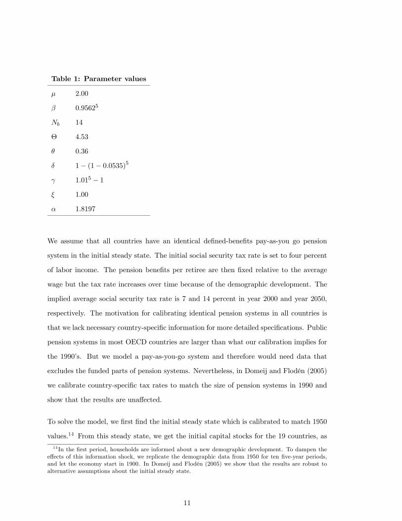
Table 1: Parameter values

µ 2.00

β 0.95625

Nb 14

Θ 4.53

θ 0.36

δ 1− (1− 0.0535)5

γ 1.015 − 1ξ 1.00

α 1.8197

We assume that all countries have an identical defined-benefits pay-as-you go pension

system in the initial steady state. The initial social security tax rate is set to four percent

of labor income. The pension benefits per retiree are then fixed relative to the average

wage but the tax rate increases over time because of the demographic development. The

implied average social security tax rate is 7 and 14 percent in year 2000 and year 2050,

respectively. The motivation for calibrating identical pension systems in all countries is

that we lack necessary country-specific information for more detailed specifications. Public

pension systems in most OECD countries are larger than what our calibration implies for

the 1990’s. But we model a pay-as-you-go system and therefore would need data that

excludes the funded parts of pension systems. Nevertheless, in Domeij and Flodén (2005)

we calibrate country-specific tax rates to match the size of pension systems in 1990 and

show that the results are unaffected.

To solve the model, we first find the initial steady state which is calibrated to match 1950

values.14 From this steady state, we get the initial capital stocks for the 19 countries, as

14 In the first period, households are informed about a new demographic development. To dampen theeffects of this information shock, we replicate the demographic data from 1950 for ten five-year periods,and let the economy start in 1900. In Domeij and Flodén (2005) we show that the results are robust toalternative assumptions about the initial steady state.

11

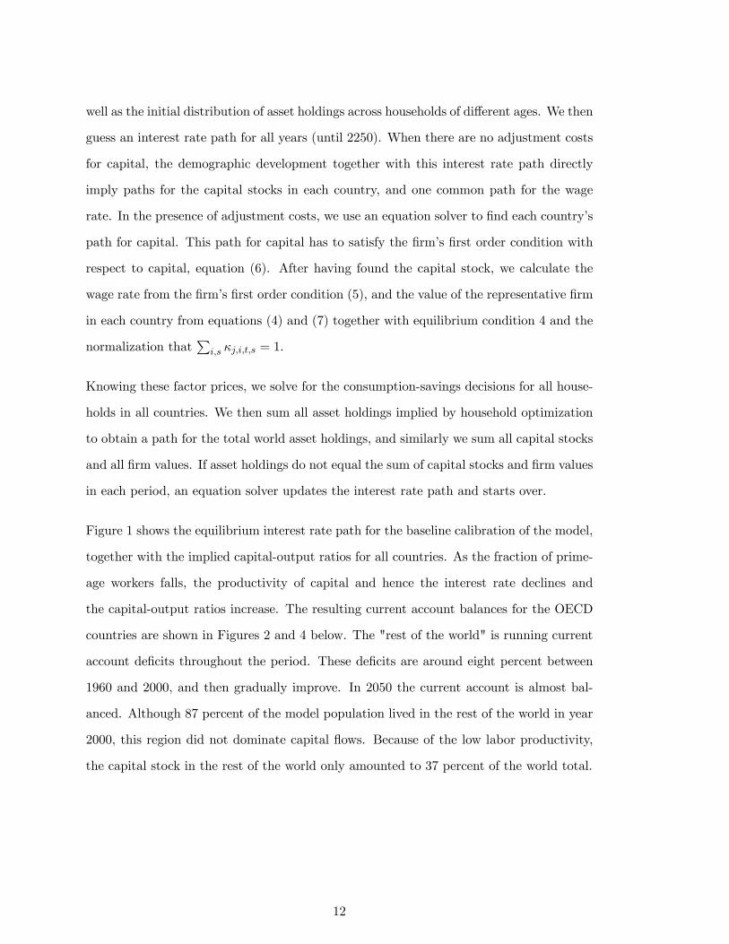
well as the initial distribution of asset holdings across households of different ages. We then

guess an interest rate path for all years (until 2250). When there are no adjustment costs

for capital, the demographic development together with this interest rate path directly

imply paths for the capital stocks in each country, and one common path for the wage

rate. In the presence of adjustment costs, we use an equation solver to find each country’s

path for capital. This path for capital has to satisfy the firm’s first order condition with

respect to capital, equation (6). After having found the capital stock, we calculate the

wage rate from the firm’s first order condition (5), and the value of the representative firm

in each country from equations (4) and (7) together with equilibrium condition 4 and the

normalization thatP

i,s κj,i,t,s = 1.

Knowing these factor prices, we solve for the consumption-savings decisions for all house-

holds in all countries. We then sum all asset holdings implied by household optimization

to obtain a path for the total world asset holdings, and similarly we sum all capital stocks

and all firm values. If asset holdings do not equal the sum of capital stocks and firm values

in each period, an equation solver updates the interest rate path and starts over.

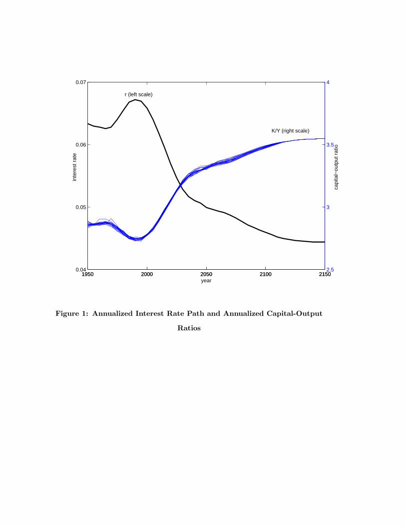
Figure 1 shows the equilibrium interest rate path for the baseline calibration of the model,

together with the implied capital-output ratios for all countries. As the fraction of prime-

age workers falls, the productivity of capital and hence the interest rate declines and

the capital-output ratios increase. The resulting current account balances for the OECD

countries are shown in Figures 2 and 4 below. The "rest of the world" is running current

account deficits throughout the period. These deficits are around eight percent between

1960 and 2000, and then gradually improve. In 2050 the current account is almost bal-

anced. Although 87 percent of the model population lived in the rest of the world in year

2000, this region did not dominate capital flows. Because of the low labor productivity,

the capital stock in the rest of the world only amounted to 37 percent of the world total.

12

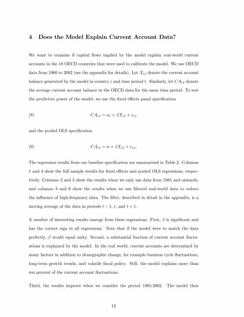
4 Does the Model Explain Current Account Data?

We want to examine if capital flows implied by the model explain real-world current

accounts in the 18 OECD countries that were used to calibrate the model. We use OECD

data from 1960 to 2002 (see the appendix for details). Let Xi,t denote the current account

balance generated by the model in country i and time period t. Similarly, let CAi,t denote

the average current account balance in the OECD data for the same time period. To test

the predictive power of the model, we use the fixed effects panel specification

(8) CAi,t = αi + βXi,t + εi,t

and the pooled OLS specification

(9) CAi,t = α+ βXi,t + εi,t.

The regression results from our baseline specification are summarized in Table 2. Columns

1 and 4 show the full sample results for fixed effects and pooled OLS regressions, respec-

tively. Columns 2 and 5 show the results when we only use data from 1985 and onwards,

and columns 3 and 6 show the results when we use filtered real-world data to reduce

the influence of high-frequency data. The filter, described in detail in the appendix, is a

moving average of the data in periods t− 1, t, and t+ 1.

A number of interesting results emerge from these regressions. First, β is significant and

has the correct sign in all regressions. Note that if the model were to match the data

perfectly, β would equal unity. Second, a substantial fraction of current account fluctu-

ations is explained by the model. In the real world, current accounts are determined by

many factors in addition to demographic change, for example business cycle fluctuations,

long-term growth trends, and volatile fiscal policy. Still, the model explains more than

ten percent of the current account fluctuations.

Third, the results improve when we consider the period 1985-2002. The model then

13

explains more of the data, 17 percent of fluctuations in the panel regression and 27 percent

in the pooled regression, and the parameter estimates are closer to unity. This can be

understood as follows. A fundamental assumption behind our work is that capital can

move freely between countries. Contrary to this assumption, Feldstein and Horioka (1980)

found that the correlation between a country’s investment and saving rate was close to

unity in a sample of OECD countries between 1960 and 1974. During the 1970’s and

1980’s, however, many countries removed restrictions on international capital flows, and

in particular the European economies became more internationally integrated. Blanchard

and Giavazzi (2002) consequently find that the correlation between investment and saving

diminished after 1975 and in particular after 1990. Consistent with these findings, we

find that the parameter estimates for the period 1960-1984 and 1985-2002 are statistically

different at the one percent level in the pooled OLS specification.

Arguably, the demographic impact on current account balances is largest at low frequen-

cies. In most regressions, we focus on the model’s ability to explain current account

fluctuations over five year intervals, thereby eliminating much of business cycle fluctua-

tions. When we reduce the impact of high-frequency fluctuations even further by filtering

the real-world data, as in columns (3) and (6), the explanatory power of the model in-

creases slightly. Furthermore, the high R2 in the pooled regressions, in particular for the

latter period, indicate that the model does not only capture fluctuations in the current

account balance over time, but that it also explains level differences between countries.

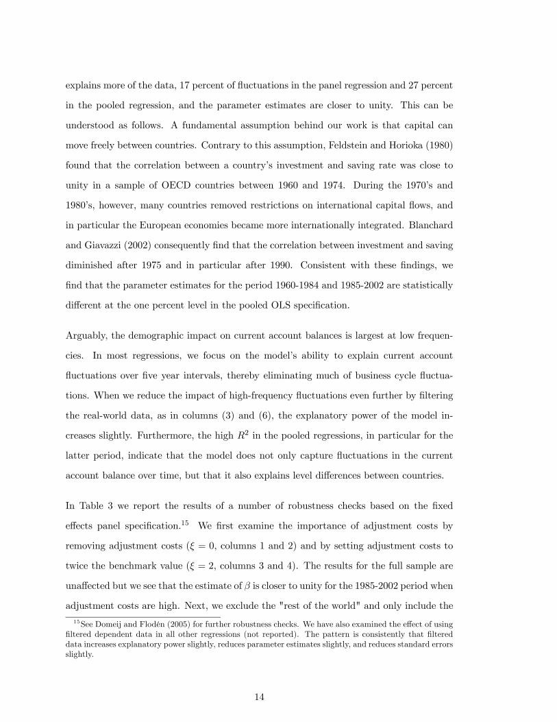
In Table 3 we report the results of a number of robustness checks based on the fixed

effects panel specification.15 We first examine the importance of adjustment costs by

removing adjustment costs (ξ = 0, columns 1 and 2) and by setting adjustment costs to

twice the benchmark value (ξ = 2, columns 3 and 4). The results for the full sample are

unaffected but we see that the estimate of β is closer to unity for the 1985-2002 period when

adjustment costs are high. Next, we exclude the "rest of the world" and only include the

15See Domeij and Flodén (2005) for further robustness checks. We have also examined the effect of usingfiltered dependent data in all other regressions (not reported). The pattern is consistently that filtereddata increases explanatory power slightly, reduces parameter estimates slightly, and reduces standard errorsslightly.

14

OECD countries in the model calibration (columns 5 and 6). The regressions now result

in less significant estimates and lower explanatory power, but the point estimates for β are

still positive and higher in the latter period. The effects of removing the pension system

(columns 7 and 8), and reducing risk aversion to unity (columns 9 and 10) are negligible.

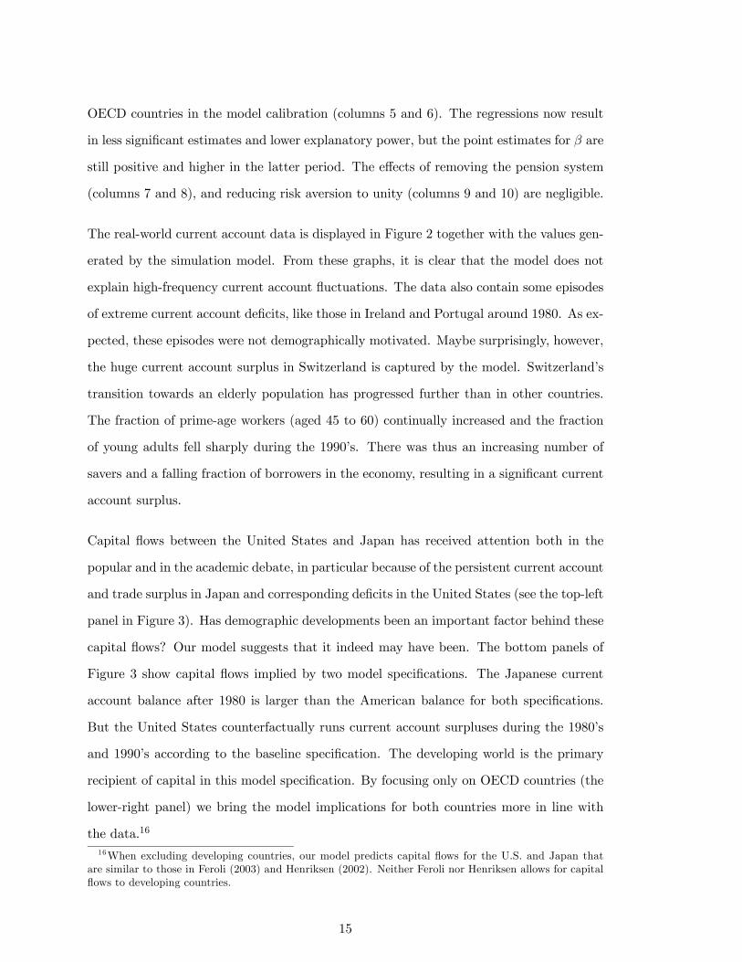
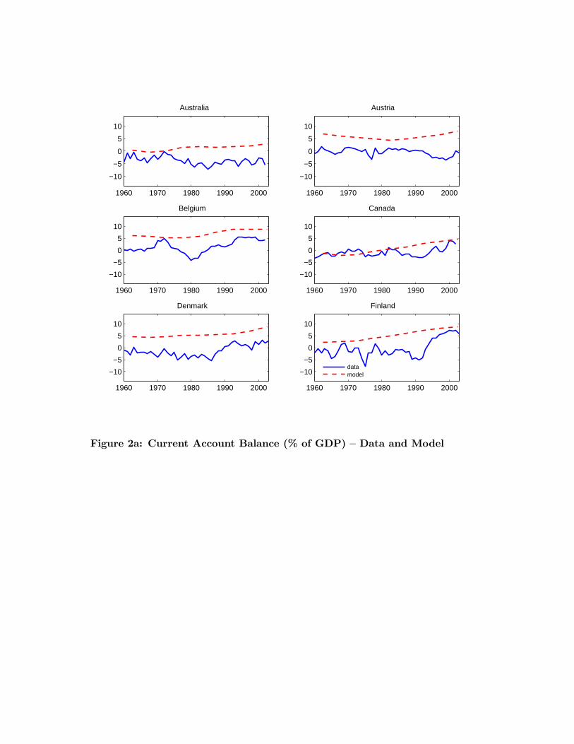
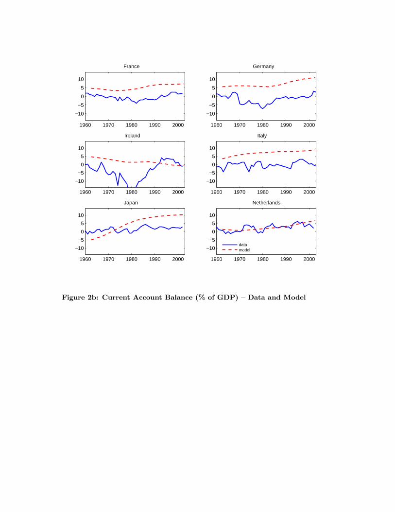
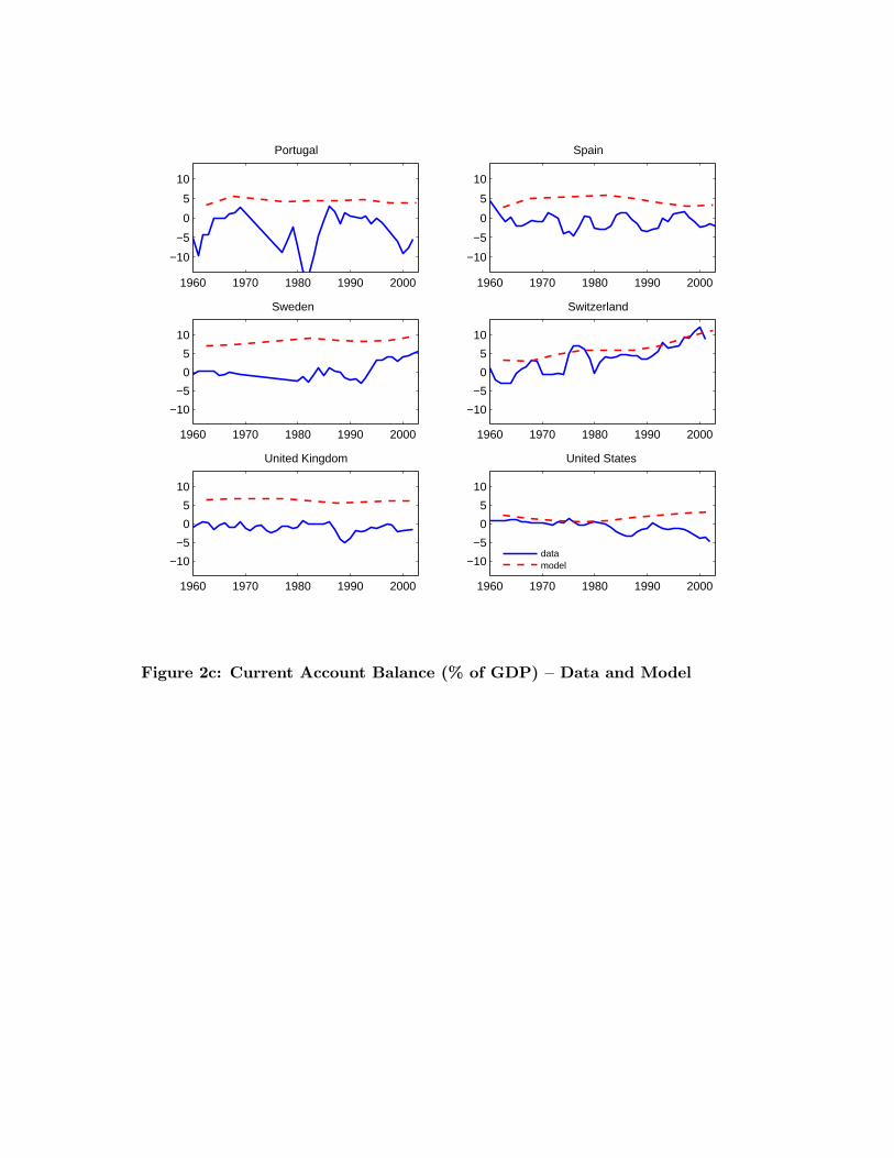
The real-world current account data is displayed in Figure 2 together with the values gen-

erated by the simulation model. From these graphs, it is clear that the model does not

explain high-frequency current account fluctuations. The data also contain some episodes

of extreme current account deficits, like those in Ireland and Portugal around 1980. As ex-

pected, these episodes were not demographically motivated. Maybe surprisingly, however,

the huge current account surplus in Switzerland is captured by the model. Switzerland’s

transition towards an elderly population has progressed further than in other countries.

The fraction of prime-age workers (aged 45 to 60) continually increased and the fraction

of young adults fell sharply during the 1990’s. There was thus an increasing number of

savers and a falling fraction of borrowers in the economy, resulting in a significant current

account surplus.

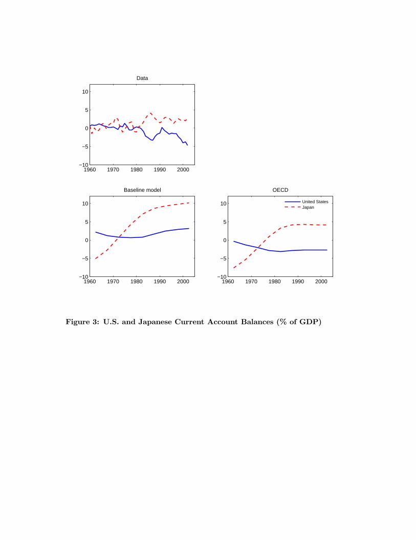
Capital flows between the United States and Japan has received attention both in the

popular and in the academic debate, in particular because of the persistent current account

and trade surplus in Japan and corresponding deficits in the United States (see the top-left

panel in Figure 3). Has demographic developments been an important factor behind these

capital flows? Our model suggests that it indeed may have been. The bottom panels of

Figure 3 show capital flows implied by two model specifications. The Japanese current

account balance after 1980 is larger than the American balance for both specifications.

But the United States counterfactually runs current account surpluses during the 1980’s

and 1990’s according to the baseline specification. The developing world is the primary

recipient of capital in this model specification. By focusing only on OECD countries (the

lower-right panel) we bring the model implications for both countries more in line with

the data.16

16When excluding developing countries, our model predicts capital flows for the U.S. and Japan thatare similar to those in Feroli (2003) and Henriksen (2002). Neither Feroli nor Henriksen allows for capitalflows to developing countries.

15

Behind any change in the current account balance, there must be corresponding changes

in savings or investment rates. To examine whether the model also explains fluctuations

in savings and investment rates we run regressions analogous to (8) and (9) but using

model data for savings or investment rates as the explanatory X variable and OECD

data on savings and investment rates as the dependent variables. The results reported in

Table 4 show that point estimates for the recent time period still are close to unity and

significantly different from zero. The model explains a smaller fraction of the variance in

these variables than in the current account balance.

5 Concluding Discussion

Theory predicts that international capital flows are determined by many factors, for ex-

ample business cycle fluctuations, long-term growth trends, and volatile fiscal policy. In

this paper we ignore all these factors and use a model where all capital flows are generated

by changes in countries’ population age structure, and find that the model can explain a

substantial fraction of capital flows at low frequencies.

We do not argue that the other factors are unimportant. For example, anticipated changes

in productivity or income may explain the current account deficits in Norway in the 1970’s,

and in Ireland and Portugal around 1980. But, allowing for productivity changes in the

model would be problematic. If we assume that such changes are perfectly predicted,

capital flows would be dramatic and unrealistic (imagine for example Japanese households

already in 1950 anticipating the country’s future productivity development). To avoid such

information problems, we have isolated the effects from demographics to capital flows.

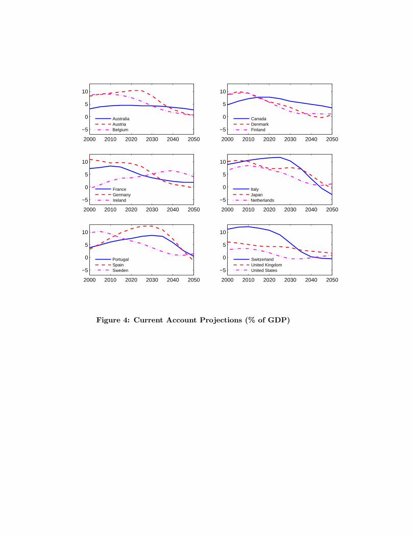
Since the model explains historical data rather well, it may also provide insights about

how the demographic development will affect capital flows in the future. Figure 4 therefore

shows current account projections based on the baseline model specification. The model

predicts current account improvements in Southern Europe and Ireland and a downward

pressure on the current accounts in the United States and Scandinavia during the coming

16

one or two decades. These capital flows are explained by the relative timing of population

aging in the different countries. The former group of countries will see an increasing

fraction of prime-age workers in the coming decades, with a peak after 2020, while the

fraction of prime-age workers has already peaked or is just about to peak in the latter

group of countries.

We want to point out that the current account projections reported in Figure 4 should

not be used as forecasts of future capital flows. Our projections focus on the direct impact

from demographics to capital flows and ignores indirect effects from policy changes, and

policy reforms will most likely be necessary in many countries if the demographic change

turns out to be as dramatic as predicted. Such reforms (for example pension reforms)

could substantially affect capital flows.17

Appendix: Data

Data for 1960-1969 are from OECD (1988) and data for 1970-2002 are from OECD (2004),

and we use current price series for all national accounts data. We calculate the investment

share (I) as (‘increase in stocks’ + ‘gross fixed capital formation’) / GDP for the 1960-1969

period, and as ‘gross capital formation’ / GDP for the 1970-2002 period. The savings rate

(S) is calculated as (GNP+ ‘net current transfers from the rest of the world’− ‘governmentfinal consumption expenditure’ − ‘private final consumption expenditure’) / GDP for the1960-1969 period, and as (GNP + ‘net current transfers from the rest of the world’ + ‘net

capital transfers from the rest of the world’ − ‘final consumption expenditure’) / GDP forthe 1970-2002 period. The current account balance as a fraction of GDP is then calculated

as CA = S − I.

In columns (3) and (6) in Table 2, we use filtered real-world data as the dependent variable.

As before, CAi,t is the average current account balance relative to GDP for that five-year

period. We then calculate CAi,t as 0.25 × CAi,t−1 + 0.50 × CAi,t + 0.25 × CAi,t+1. If

17Börsch-Supan et al. (2004) examine how pension reforms would affect future capital flows.

17

the value for CAi,t is missing, we set a missing value for CAi,t, but if the value for

CAi,t−1 or CAi,t+1 is missing, we use the available observations and adjust the weights.

For example, if t = 1960 values for t = 1955 are missing and we calculate CAi,1960 =

(0.50× CAi,1960 + 0.25× CAi,1965) /0.75. Columns (3) and (6) report results with CAi,t

as the dependent variable.

18

References

Attanasio, O. and G. Violante, "The Demographic Transition in Closed and Open Econ-

omy: A Tale of Two Regions," Working Paper 412, Research Department, Inter-

American Development Bank, Washington, 2000.

Auerbach, A.J. and L.J. Kotlikoff, Dynamic Fiscal Policy (Cambridge: Cambridge Uni-

versity Press, 1987).

Auerbach, A.J., L.J. Kotlikoff, R.P. Hagemann and G. Nicoletti, "The Economic Dynam-

ics of an Ageing Population: The Case of Four OECD Countries," Working Paper

No. 62, Department of Economics and Statistics, OECD, Paris, 1989.

Backus, D.K., P.J. Kehoe and F.E. Kydland, "International Business Cycles: Theory and

Evidence," in T. F. Cooley, ed., Frontiers of Business Cycle Research (Princeton:

Princeton University Press, 1995).

Bell, F.C., A.H. Wade and S.C. Goss, "Life Tables for the United States Social Security

Area 1900-2080," Actuarial Study No. 107, U.S. Department of Health and Human

Services, 1992.

Blanchard, O. and F. Giavazzi, "Current Account Deficits in the Euro Area: The End

of the Feldstein Horioka Puzzle?," Brookings Papers on Economic Activity (2002:2),

147-209.

Börsch-Supan, A., A. Ludwig and J. Winter, "Aging, Pension Reform, and Capital Flows:

A Multi-Country Simulation Model," mimeo, Mannheim Research Institute for the

Economics of Aging, 2004.

Brooks, R., "Population Aging and Global Capital Flows in a Parallel Universe," IMF

Staff Papers 50 (2003), 200-221.

Cooley, T.F. and E.C. Prescott, "Economic Growth and Business Cycles", in T. F.

Cooley, ed., Frontiers of Business Cycle Research (Princeton: Princeton University

Press, 1995).

19

Cutler, D.M., J.M. Poterba, L.M. Sheiner and L.H. Summers, "An Aging Society: Op-

portunity or Challenge?," Brookings Papers on Economic Activity (1990:1), 1-73.

Domeij, D. and M. Flodén, "More on Population Aging and International Capital Flows,"

mimeo, Stockholm School of Economics, 2005.

Eberly, J.C., "International Evidence on Investment and Fundamentals," European Eco-

nomic Review 41 (1997), 1055-1078.

Fair, R.C. and K.M. Dominguez, "Effects of the Changing U.S. Age Distribution on

Macroeconomic Equations," American Economic Review 81 (1991), 1276-1294.

Feldstein, M. and C. Horioka, "Domestic Saving and International Capital Flows," Eco-

nomic Journal 90 (1980), 314-329.

Fernández-Villaverde, J. and D. Krueger, "Consumption over the Life Cycle: Some Facts

from the Consumer Expenditure Survey Data," mimeo, University of Pennsylvania,

2003.

Feroli, M., "Capital Flows Among the G-7 Nations: A Demographic Perspective," Fi-

nance and Economics Discussion Series 2003-54, Board of Governors of the Federal

Reserve System, 2003.

Flodén, M., "Public Saving and Policy Coordination in Aging Economies," Scandinavian

Journal of Economics 105 (2003), 379-400.

Fullerton, H.N. Jr., "Labor Force Participation: 75 Years of Change, 1950-98 and 1998-

2025," Monthly Labor Review 122 (1999), 3-12.

Hansen, G.D., "The Cyclical and Secular Behaviour of the Labor Input: Comparing

Efficiency Units and Hours Worked," Journal of Applied Econometrics 8 (1993),

71-80.

Henriksen, E.R., "A Demographic Explanation of U.S. and Japanese Current Account

Behavior," mimeo, Carnegie Mellon University, 2002.

20

Higgins, M., "Demography, National Savings, and International Capital Flows," Inter-

national Economic Review 39 (1998), 343-369.

Higgins, M. and J.G. Williamson, "Age Structure Dynamics in Asia and Dependence on

Foreign Capital," Population and Development Review 23 (1997), 261-293.

Lane, P.R. and G.M. Milesi-Ferretti, "Long-Term Capital Movements", NBER Macro-

economics Annual (2001:1), 73-116.

Maddison, A., The World Economy: A Millennial Perspective, (Paris: OECD Develop-

ment Centre Studies, 2001).

OECD, The OECD List of Social Indicators, (Paris: OECD, 1982).

OECD, National Accounts 1960-1986: Main Aggregates, Volume I, (Paris: OECD, 1988).

OECD, Annual National Accounts: Main Aggregates, Volume I, Release 02, (Paris:

OECD, 2004).

United Nations, The 2002 Revision Population Database, http://esa.un.org/unpp/, 2002.

World Bank, 1995, Nehru and Dhareshwa Dataset, The World Bank Group, Washington

21

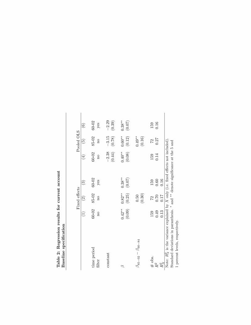
Table2:Regressionresultsforcurrentaccount

Baselinespecification

Fixedeffects

PooledOLS

(1)

(2)

(3)

(4)

(5)

(6)

timeperiod

60-02

85-02

60-02

60-02

85-02

60-02

filter

nono

yes

nono

yes

constant

−2.38−3

.15−2

.29

(0.44)

(0.78)

(0.39)

β0.42∗∗

0.82∗∗

0.38∗∗

0.40∗∗

0.60∗∗

0.38∗∗

(0.09)

(0.25)

(0.07)

(0.08)

(0.12)

(0.07)

β85−02−β60−84

0.50

0.49∗∗

(0.30)

(0.16)

#obs.

159

72159

159

72159

R2

0.49

0.70

0.60

0.14

0.27

0.16

R2 X

0.13

0.17

0.16

Note:

R2 Xisthevarianceexplainedby

Xonly(i.e.fixedeffectsnotincluded).

Standarddeviationsinparanthesis.∗and∗∗denotesignificanceatthe5and

1percentlevels,respectively.

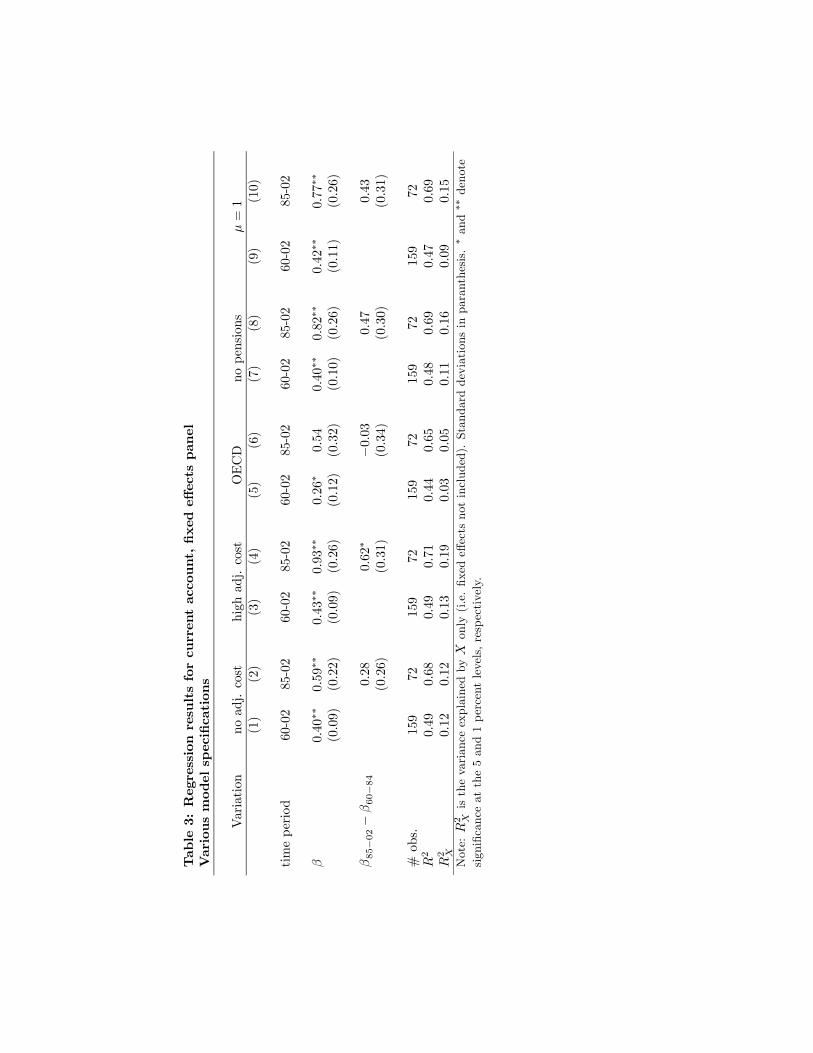
Table3:Regressionresultsforcurrentaccount,fixedeffectspanel

Variousmodelspecifications

Variation

noadj.cost

highadj.cost

OECD

nopensions

µ=1

(1)

(2)

(3)

(4)

(5)

(6)

(7)

(8)

(9)

(10)

timeperiod

60-02

85-02

60-02

85-02

60-02

85-02

60-02

85-02

60-02

85-02

β0.40∗∗

0.59∗∗

0.43∗∗

0.93∗∗

0.26∗

0.54

0.40∗∗

0.82∗∗

0.42∗∗

0.77∗∗

(0.09)

(0.22)

(0.09)

(0.26)

(0.12)

(0.32)

(0.10)

(0.26)

(0.11)

(0.26)

β85−02−β60−84

0.28

0.62∗

−0.03

0.47

0.43

(0.26)

(0.31)

(0.34)

(0.30)

(0.31)

#obs.

159

72159

72159

72159

72159

72R2

0.49

0.68

0.49

0.71

0.44

0.65

0.48

0.69

0.47

0.69

R2 X

0.12

0.12

0.13

0.19

0.03

0.05

0.11

0.16

0.09

0.15

Note:R2 Xisthevarianceexplainedby

Xonly(i.e.fixedeffectsnotincluded).Standarddeviationsinparanthesis.∗and∗∗denote

significanceatthe5and1percentlevels,respectively.

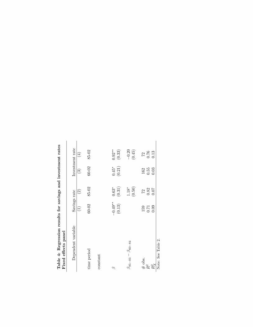
Table4:Regressionresultsforsavingsandinvestmentrates

Fixed

effectspanel

Dependentvariable

Savingsrate

Investmentrate

(1)

(2)

(3)

(4)

timeperiod

60-02

85-02

60-02

85-02

constant

β−0

.49∗∗

0.63∗

0.45∗

0.92∗∗

(0.13)

(0.31)

(0.21)

(0.33)

β85−03−β60−84

1.18∗

−0.20

(0.50)

(0.45)

#obs.

159

72162

72R2

0.71

0.82

0.55

0.76

R2 X

0.09

0.07

0.03

0.13

Note:SeeTable2.

1950 2000 2050 2100 21500.04

0.05

0.06

0.07

year1950 2000 2050 2100 2150

2.5

3

3.5

4

r (left scale)

K/Y (right scale)

capi

tal−

outp

ut r

atio

inte

rest

rat

e

Figure 1: Annualized Interest Rate Path and Annualized Capital-Output

Ratios

1960 1970 1980 1990 2000

−10

−5

0

5

10

Australia

1960 1970 1980 1990 2000

−10

−5

0

5

10

Austria

1960 1970 1980 1990 2000

−10

−5

0

5

10

Belgium

1960 1970 1980 1990 2000

−10

−5

0

5

10

Canada

1960 1970 1980 1990 2000

−10

−5

0

5

10

Denmark

1960 1970 1980 1990 2000

−10

−5

0

5

10

Finland

datamodel

Figure 2a: Current Account Balance (% of GDP) — Data and Model

1960 1970 1980 1990 2000

−10

−5

0

5

10

France

1960 1970 1980 1990 2000

−10

−5

0

5

10

Germany

1960 1970 1980 1990 2000

−10

−5

0

5

10

Ireland

1960 1970 1980 1990 2000

−10

−5

0

5

10

Italy

1960 1970 1980 1990 2000

−10

−5

0

5

10

Japan

1960 1970 1980 1990 2000

−10

−5

0

5

10

Netherlands

datamodel

Figure 2b: Current Account Balance (% of GDP) — Data and Model

1960 1970 1980 1990 2000

−10

−5

0

5

10

Portugal

1960 1970 1980 1990 2000

−10

−5

0

5

10

Spain

1960 1970 1980 1990 2000

−10

−5

0

5

10

Sweden

1960 1970 1980 1990 2000

−10

−5

0

5

10

Switzerland

1960 1970 1980 1990 2000

−10

−5

0

5

10

United Kingdom

1960 1970 1980 1990 2000

−10

−5

0

5

10

United States

datamodel

Figure 2c: Current Account Balance (% of GDP) — Data and Model

1960 1970 1980 1990 2000−10

−5

0

5

10

Data

1960 1970 1980 1990 2000−10

−5

0

5

10

Baseline model

1960 1970 1980 1990 2000−10

−5

0

5

10

OECD

United StatesJapan

Figure 3: U.S. and Japanese Current Account Balances (% of GDP)

2000 2010 2020 2030 2040 2050

−5

0

5

10

AustraliaAustriaBelgium

2000 2010 2020 2030 2040 2050

−5

0

5

10

CanadaDenmarkFinland

2000 2010 2020 2030 2040 2050

−5

0

5

10

FranceGermanyIreland

2000 2010 2020 2030 2040 2050

−5

0

5

10

ItalyJapanNetherlands

2000 2010 2020 2030 2040 2050

−5

0

5

10

PortugalSpainSweden

2000 2010 2020 2030 2040 2050

−5

0

5

10

SwitzerlandUnited KingdomUnited States

Figure 4: Current Account Projections (% of GDP)