


Languages
Pages
Legal


Popula'on Structure
02-‐710 Computa.onal Genomics
Seyoung Kim


What is Popula'on Structure?
• Popula.on Structure – A set of individuals characterized by some measure of gene.c
dis.nc.on
– A “popula.on” is usually characterized by a dis.nct distribu.on over genotypes
– Example Genotypes aa aA AA
Popula.on 1 Popula.on 2
3

Mo'va'on • Reconstruc'ng individual ancestry: The Genographic Project – hJps://genographic.na.onalgeographic.com/
4
Studying human migra.on out of Africa

Mo'va'on
• Study of various traits (e.g., lactose intolerance)
5

Overview
• Background – Hardy-‐Weinberg Equilibrium
– Gene.c driX – Wright’s FST
• Inferring popula.on structure from genotype data – Model-‐based method: Structure (Falush et al., 2003) for admixture
model, linkage model
– Principal component analysis (PaJerson et al., PLoS Gene.cs 2006)
6

Hardy-‐Weinberg Equilibrium
• Hardy-‐Weinberg Equilibruim – Under random ma.ng, both allele and genotype frequencies in a
popula.on remain constant over genera.ons.
– Assump.ons of the standard random ma.ng • Diploid organism
• Sexual reproduc.on • Nonoverlapping genera.ons • Random ma.ng
• Large popula.on size • Equal allele frequencies in the sexes • No migra.on/muta.on/selec.on
– Chi-‐square test for Hardy-‐Weinberg equilibrium
7

Genotype/Allele Frequencies in the Current Genera'on
• Genotype frequencies in the current genera.on – D: frequency for AA – H: frequency for Aa – R: frequency for aa
– D + H + R = 1.0
• Allele frequencies in the current genera.on – p: : frequency of A
• p = (2D + H) / 2 = D + H/2 – q: frequency of a
• q = (2R + H) / 2 = R + H/2
8

Genotype/Allele Frequencies of the Offspring
• Genotype frequencies in the offspring – D’: frequency for AA
• D’ = p2 – H’: frequency for Aa
• H’ = pq + pq = 2pq – R’: frequency for aa
• R’ = q2
• Allele frequencies in the offspring – p’ = (2D’ + H’)/2 = (2p2 + 2pq)/2 = p(p + q) = p
– q’ = (2R’ + H’)/2 = (2q2 + 2pq)/2 = q(q + p) = q
9
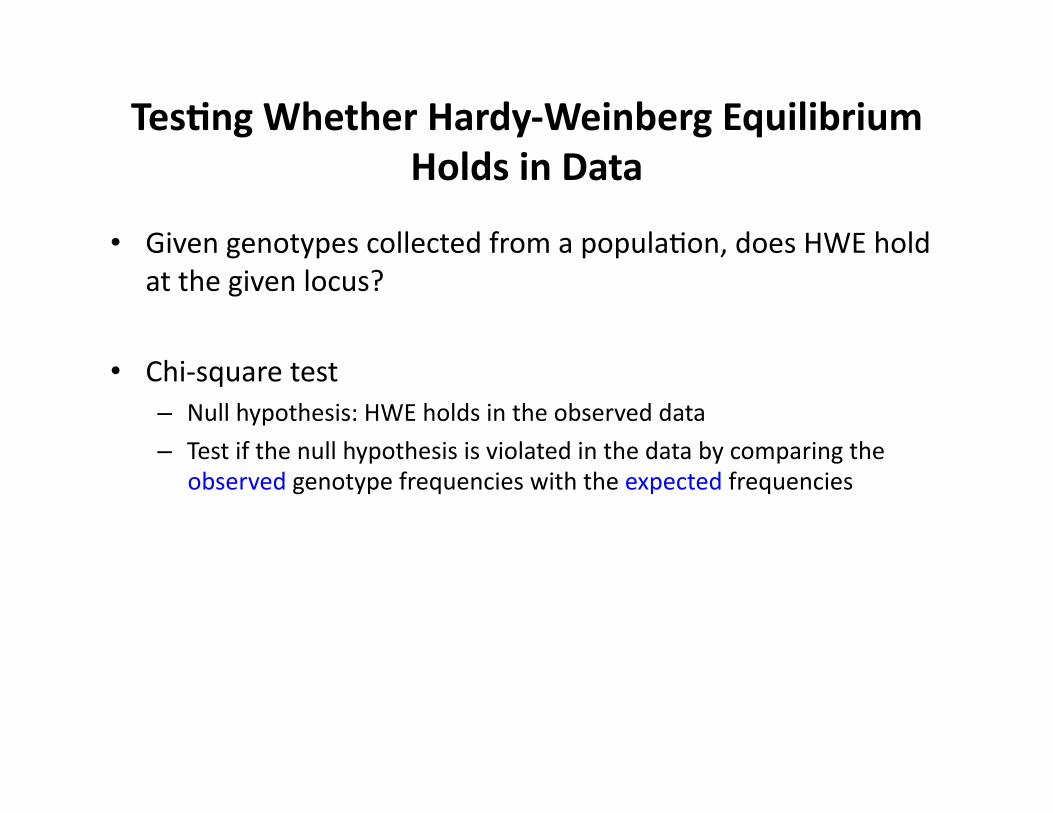
Tes'ng Whether Hardy-‐Weinberg Equilibrium Holds in Data
• Given genotypes collected from a popula.on, does HWE hold at the given locus?
• Chi-‐square test – Null hypothesis: HWE holds in the observed data
– Test if the null hypothesis is violated in the data by comparing the observed genotype frequencies with the expected frequencies

Tes'ng Whether Hardy-‐Weinberg Equilibrium Holds
Genotype AA Aa aa Total
Observed 224 64 6 294
Expected ? ? ? 294
Con.ngency table for chi-‐square test
€
p =224 × 2 + 64294 × 2
= 0.871
q =1− p = 0.129
Step 1: Compute allele frequencies from the observed data

Tes'ng Whether Hardy-‐Weinberg Equilibrium Holds
Genotype AA Aa aa Total
Observed 224 64 6 294
Expected 222.9 66.2 4.9 294
Step 3: Compute the test sta.s.c (degree of freedom 1)
€
χ2 =(observed - expected)2
expected∑
=(224 − 222.9)2
222.9+(64 − 66.2)2
66.2+(6 − 4.9)2
4.9= 0.32
€
p =224 × 2 + 64294 × 2
= 0.871
q =1− p = 0.129
Step 1: Compute allele frequencies from the observed data
€
Expected(AA) = p2n = 0.87072 × 294 = 222.9Step 2: Compute the expected genotype frequencies
Con.ngency table for chi-‐square test

Hardy-‐Weinberg Equilibrium in Prac'ce
• HWE oXen does not hold in reality because of the viola.on of the assump.ons (i.e., random ma.ng, no selec.on, etc.)
• Even when the assump.ons for HWE hold, in reality, allele frequencies change over genera.ons because of the random fluctua.on – gene.c driX!

Gene'c DriL
• The change in allele frequencies in a popula.on due to random sampling
• All muta.ons eventually driX to allele frequency 0 or 1 over .me
• Neutral process unlike natural selec.on – But gene.c driX can eliminate an
allele from the given popula.on.
• The effect of gene.c driX is larger in a small popula.on
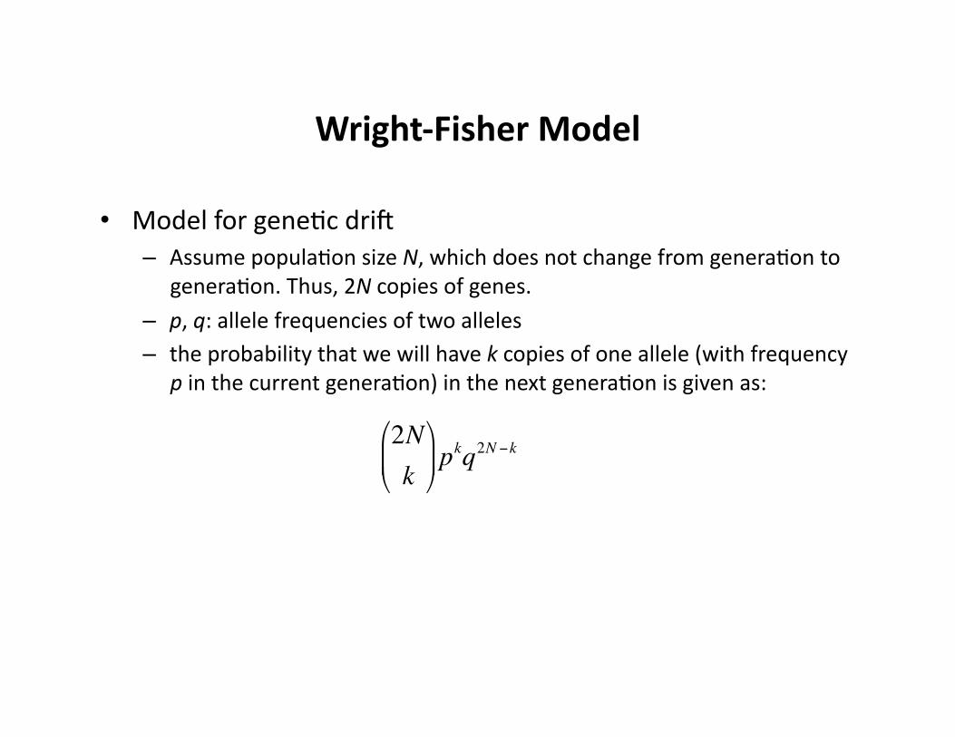
Wright-‐Fisher Model
• Model for gene.c driX – Assume popula.on size N, which does not change from genera.on to
genera.on. Thus, 2N copies of genes.
– p, q: allele frequencies of two alleles – the probability that we will have k copies of one allele (with frequency
p in the current genera.on) in the next genera.on is given as:
€
2Nk
⎛
⎝ ⎜
⎞
⎠ ⎟ pkq2N −k

Popula'on Divergence and Admixture
• Popula.on divergence – Once a single popula.on is separated into two subpopula.ons, each of
the subpopula.ons will be subject to its own gene.c driX and natural selec.on
– Popula.on divergence creates different allele frequencies for the same loci across different popula.ons
• Admixture – Two previously separated popula.ons migrate/mate to form an
admixed popula.on

Scenarios of How Popula'ons Evolve
17
Admixing Single popula.on
Divergence

Popula'on Divergence
• Wright’s FST – Sta.s.cs used to quan.fy the extent of divergence among mul.ple
popula.ons rela.ve to the overall gene.c diversity
– Summarizes the average devia.on of a collec.on of popula.ons away from the mean
– FST = Var(pk)/p’(1-p’) • p’: the overall frequency of an allele across all subpopulations • pk : the allele frequency within population k
18

Overview
• Background – Hardy-‐Weinberg Equilibrium
– Gene.c driX – Wright’s FST
• Inferring popula.on structure from genotype data – Model-‐based method: Structure (Falush et al., 2003) for admixture
model, linkage model
– Principal component analysis (PaJerson et al., PLoS Gene.cs 2006)
19
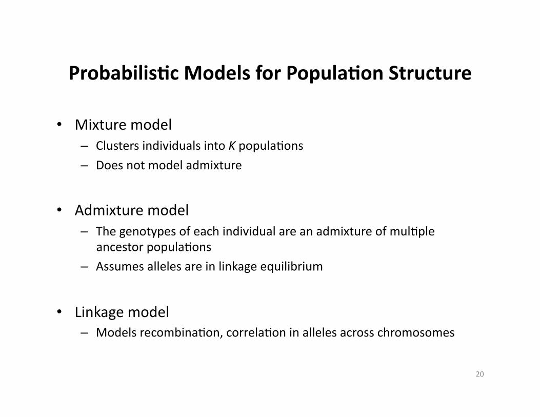
Probabilis'c Models for Popula'on Structure
• Mixture model – Clusters individuals into K popula.ons – Does not model admixture
• Admixture model – The genotypes of each individual are an admixture of mul.ple
ancestor popula.ons
– Assumes alleles are in linkage equilibrium
• Linkage model – Models recombina.on, correla.on in alleles across chromosomes
20

Structure Model
• Hypothesis: Modern popula.ons are created by an intermixing of ancestral popula.ons.
• An individual’s genome contains contribu.ons from one or more ancestral popula.ons.
• The contribu.ons of popula.ons can be different for different individuals.
• Other assump.ons – No linkage disequilbrium
– Markers are i.i.d (independent and iden.cally distributed)
21

Modeling Admixture N individuals
L loci
K ancestral popula.ons
L loci
Allele frequencies at each locus for each ancestral popula.on
Genotype Data
N individuals
L loci
Admixed Genome
N individuals K popula.ons
Individuals’ ancestry propor.ons (Column sum to 1)
0.2 0.3 0.5

STRUCTURE for Modeling Admixture
X
N individuals
L loci
K ancestral popula.ons
L loci
Allele frequencies at each locus for each ancestral popula.on
Genotype Data
Z
N individuals
L loci
Admixed Genome
N individuals K popula.ons
Individuals’ ancestry propor.ons (Column sum to 1)
θn : nth individual
β1 β2 β3
0.2 0.3 0.5

Genera've Model for STRUCTURE
• βk : Allele frequencies for popula.on k at L loci
• For each individual n=1,…,N – Sample θn from Dirichlet(α)
– For each locus i=1,…,L • Sample Zi,n from Mul.nomial(θn)
• Sample Xi,n from βk,i for the popula.on chosen by k=Zi,n
24
βk λ
Xi,n
Zi,n
θn
i=1…L
n=1…N
α
k=1…K
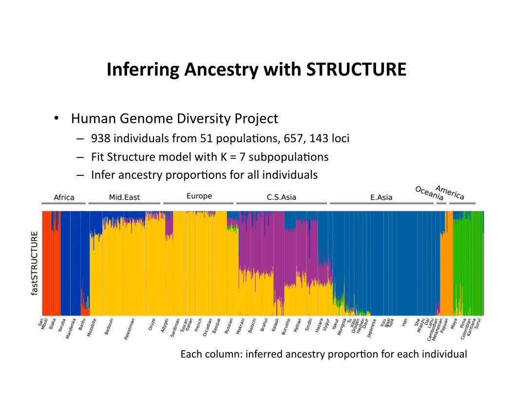
Inferring Ancestry with STRUCTURE
• Human Genome Diversity Project – 938 individuals from 51 popula.ons, 657, 143 loci
– Fit Structure model with K = 7 subpopula.ons – Infer ancestry propor.ons for all individuals
Each column: inferred ancestry propor.on for each individual

Structure Model
• Advantages – Genera.ve process
• Explicit model of admixture – Meaningful interpretable results
– Clustering is probabilis.c • Models uncertainty in clusters or popula.on labels
• Disadvantages – Alleles are same in ancestral and modern popula.ons
– No models of muta.on, recombina.on
26

Extending Structure to Model Linkage
27
βki =1…I λ
xI,n
zI,n
θn
n=1…N
α
x1,n
z1,n
x2,n
z2,n …
k=1…K
• From admixture model, replace the assump.on that the ancestry labels Zil for individual i, locus l are independent with the assump.on that adjacent Zil are correlated.
• Use Poisson process to model the correla.on between neighboring alleles – dl : distance between locus l and
locus l+1 – r: recombina.on rate

Extending Structure to Model Linkage
• As recombina.on rate r goes to infinity, all loci become independent and linkage model becomes admixture model.
• Recombina.on rate r can be viewed as being related to the number of genera.ons since admixture occurred.
• Use MCMC algorithm or varia.onal algorithms to fit the unkown parameters.
28

Neighbour-‐joining Phylogene'c Trees from the Structural Maps

Overview
• Background – Hardy-‐Weinberg Equilibrium
– Gene.c driX – Wright’s FST
• Inferring popula.on structure from genotype data – Model-‐based method: Structure (Falush et al., 2003) for admixture
model, linkage model
– Principal component analysis (PaJerson et al., PLoS Gene.cs 2006)
30

Low-‐dimensional Projec'ons
• Gene.c data is very large – Number of markers may range from a few hundreds to hundreds of
thousands – Thus each individual is described by a high-‐dimensional vector of marker
configura.ons – A low-‐dimensional projec.on of each individual allows easy visualiza.on
• Technique used – Factor analysis – Many sta.s.cal methods exist – ICA, PCA, NMF etc. – Principal Components Analysis (next slide)
• Usually projected to 2 dimensions to allow visualiza.on
31

Matrix Factoriza'on and Popula'on Structure
• Matrix factoriza.on for learning popula.on structure
Genotype Data (NxL matrix)
N: number of samples L: number of loci
Individuals’ ancestry propor.ons (NxK matrix) K: number of subpopula.ons
Subpopula.on Allele Frequencies (KxL matrix) = x
32

Principal Component Analysis to Reveal Popula'on Structure
• Genotype data X – N x L matrix for N individuals and L loci
– Normalize each column of the genotype data matrix
• Perform PCA on the covariance matrix (1/N)XX’ – K principal components with top eigenvalues capture the ancestry
informa.on

Popula'on Structure In Europe
• Apply PCA to genotype data from 197, 146 loci in 1, 387 European individuals
• Each individual is represented in two dimensions using top two principle components
• 2-‐dim projec.ons reflect the geographic regions in the map quite well

Comparison of Different Methods
PCA Model-‐based Clustering
Advantages • Easy visualiza.on • Genera.ve process that explicitly models admixture • Clustering is probabilis.c: it is possible to assign confidence level of clusters
Disadvantages • No intui.on about underlying processes
• Computa.onally more demanding • Based on assump.ons of evolu.onary models: • Structure: No models of muta.on, recombina.on • Recombina.on added in extension linkage model by Falush et al.
35

Summary
• Gene.c varia.on data can be used to infer various aspects of popula.on history such as popula.on divergence admixture.
• HWE describes the theore.cal allele frequencies in the ideal situa.on.
• Gene.c driX and natural selec.on can change allele frequencies from genera.on to genera.on.
• Model-‐based methods such as Structure or matrix-‐factoriza.on methods can be used to infer popula.on structure from genotype data.
Top Related