


Languages
Pages
Legal

Planar Timoshenko-like model for multilayer non-prismaticbeams
Giuseppe Balduzzi . Mehdi Aminbaghai . Ferdinando Auricchio . Josef Fussl
Received: 12 August 2016 / Accepted: 20 December 2016
� The Author(s) 2017. This article is published with open access at Springerlink.com
Abstract This paper aims at proposing aTimoshenko-
likemodel forplanarmultilayer (i.e., non-homogeneous)
non-prismatic beams. Themain peculiarity ofmultilayer
non-prismatic beams is a non-trivial stress distribution
within the cross-section that, therefore, needs a more
careful treatment. In greater detail, the axial stress
distribution is similar to the one of prismatic beams and
can be determined through homogenization whereas the
shear distribution is completely different from prismatic
beams and depends on all the internal forces. The
problem of the representation of the shear stress
distribution is overcame by an accurate procedure that
is devised on the basis of the Jourawsky theory. The
paper demonstrates that the proposed representation of
cross-section stress distribution and the rigorous proce-
dure adopted for the derivation of constitutive, equilib-
rium, and compatibility equations lead to Ordinary
Differential Equations that couple the axial and the shear
bending problems, but allow practitioners to calculate
both analytical and numerical solutions for almost
arbitrary beam geometries. Specifically, the numerical
examples demonstrate that the proposed beam model is
able to predict displacements, internal forces, and
stresses very accurately and with moderate computa-
tional costs. This is also valid for highly heterogeneous
beams characterized by thin and extremely stiff layers.
Keywords Non-homogeneous non-prismatic beam �Tapered beam � Beam of variable cross-section �First order beam model � Arch shaped beam
1 Introduction
According to the terminology introduced by Balduzzi
et al. (2016), the definition multilayer non-prismatic
beam refers to a continuous body made of layers of
different homogeneous materials, in which the geom-
etry of each layer can vary arbitrarily along the
prevailing dimension of the beam. Both researchers
and practitioners are interested in non-prismatic
beams since they allow to reach extremely important
optimization goals such as the desired strength with
the least material usage. Furthermore, multilayer non-
prismatic beams are nowadays more and more
employed in different engineering fields since the
workability of materials (like steel, aluminum, com-
posites, wooden or plastic products) and modern
production technologies (e.g., automatic welding
machines, 3D printers) allow to manufacture elements
with complex geometry without a significant increase
of production costs. As an example, the technologies
G. Balduzzi (&) � M. Aminbaghai � J. Fussl
Institute for Mechanics of Materials and Structures
(IMWS), Vienna University of Technology, Karlsplatz
13/202, 1040 Vienna, Austria
e-mail: [email protected]
F. Auricchio �Department of Civil Engineering and Architecture
(DICAr), University of Pavia, Via Ferrata 3, 27100 Pavia,
Italy
123
Int J Mech Mater Des
DOI 10.1007/s10999-016-9360-3
for the manufacturing of wooden or composite
beams allow to produce bodies made of materials
with different mechanical properties (Frese and
Blaß 2012). Furthermore, existing elementary
model assumptions include that steel and aluminum
beams with I or H cross-section behave under the
hypothesis of plane stress whereas the variable beam
depth is considered by proportional variation of the
different mechanical properties within the cross-
section (Schreyer 1978; Li and Li 2002; Shooshtari
and Khajavi 2010). In both cases, a planar model
capable to tackle multilayer non-prismatic beams
i.e., the object of this document, represents a
necessary tool for the modeling and first design of
such bodies as well as the starting point for the
development of more refined 3D beam models.
Furthermore, the usage of optimized non-pris-
matic beams for several engineering applications
leads the investigation and the modeling of their
behavior to be a critical step for both researchers
and practitioners. First and foremost, the possibility
to optimize the behavior of non-prismatic beams is
a significant advantage of these particular structural
elements, but, at the same time, this must be treated
with caution. As an example, let us consider a non-
prismatic beam designed in order to exploit exactly
the desired material strength in every cross-section
of the beam according to a performed sophisticated
analysis. On the one hand, such an optimization
reduces the cross-section sizes and saves material
but, on the other hand, it reduces also the structure
robustness since all the cross-sections are near to
their limit states. In particular, every small varia-
tion of the stress distribution not caught by the
analysis could lead to premature failure or to
serviceability problems of the structural element
(Paglietti and Carta 2007, 2009; Beltempo et al.
2015b). Finally, optimization processes are often
based on recursive analysis (see e.g., Allaire et al.
1997; Lee et al. 2012). Therefore, the availability
of models that are simultaneously accurate and
computationally cheap is a crucial aspect for
optimized structure designers since it allows to
reduce significantly the costs. As a consequence,
also nowadays the development of effective and
accurate models for non-prismatic structural ele-
ments represents a crucial research field continu-
ously seeking for new contributions.
1.1 Literature review
With respect to planar non-prismatic beam modeling,
several researchers (Bruhns 2003; Hodges et al. 2010;
Balduzzi et al. 2016) have shown with different
strategies that the main effect of the cross-section
variation is a non-trivial stress distribution. Besides,
the influence of cross-section variation on stress
distributions can be predicted by exploiting several
analytical solutions of the 2D elastic problem for an
infinite long wedge known since the first half of the
past century (Atkin 1938; Timoshenko and Goodier
1951). In particular, the equilibrium on lateral surfaces
requires that shear at the cross-section boundaries is
not vanishing, but must be proportional to the axial
stress and the boundary slope (Hodges et al. 2010).
Therefore, the shear distribution not only depends on
the vertical internal force V as usual for prismatic
beams, but also on the bending moment M and the
horizontal internal force H determining the magnitude
of axial stresses (Bruhns 2003, Section3.5).
As a consequence of the non-trivial stress distribu-
tion, also the beams’ shear strain depends on all the
internal forces H, V, and M and, due to the symmetry
of constitutive relations, both the curvature and the
beams’ axial strain depend on the vertical internal
force V (Balduzzi et al. 2016). The numerical exam-
ples discussed by Balduzzi et al. (2016) demonstrate
that the so far introduced relations deeply influence the
whole beam behavior and can not be neglected.
Furthermore, they confirm that non-prismatic beam-
models differ from prismatic ones not only in terms of
variable cross-section area and inertia, but they
especially result in more complex relations between
the independent variables.
A diffused approach for non-prismatic beam mod-
eling consists in using prismatic beam Ordinary
Differential Equations (ODEs) and assuming that the
cross-section area and inertia vary along the beam axis
(Portland Cement Associations 1958; Timoshenko
and Young 1965; Romano and Zingone 1992; Fried-
man and Kosmatka 1993; Shooshtari and Khajavi
2010; Trinh and Gan 2015;Maganti and Nalluri 2015),
neglecting the effects of boundary equilibrium on
stress distributions and the resulting non trivial
constitutive relations. The so far introduced approach
received criticisms since the sixties of the past century
(Boley 1963; Tena-Colunga 1996) and, as a conse-
G. Balduzzi et al.
123
quence, several researchers propose alternative strate-
gies trying to improve the non-prismatic beam mod-
eling (El-Mezaini et al. 1991; Vu-Quoc and Leger
1992; Tena-Colunga 1996). Extending for a moment
the discussion to plates, it is worth noticing that the
idea of using variable stiffness for accounting the
effects of taper is quite diffused (Edwin Sudhagar
et al. 2015; Susler et al. 2016), but enhanced modeling
approaches exist also for this class of bodies (Ra-
jagopal and Hodges 2015). Further problems that
affect non-prismatic beam models, reducing even
more their effectiveness, come from the use of coarse
numerical techniques for the solution of beam model
equations e.g., the attempts to use prismatic beam
Finite Element (FE) in order to model non-prismatic
beams (Banerjee andWilliams 1985, 1986; Tong et al.
1995; Liu et al. 2016).
To the author’s knowledge, the most enhanced
modeling approaches that seem capable to overcome all
the so far discussed limitations have been presented by
Rubin (1999), Hodges et al. (2008, 2010), Auricchio
et al. (2015), Beltempo et al. (2015a), and Balduzzi
et al. (2016). In greater detail, Rubin (1999), Hodges
et al. (2008, 2010) limit their investigations to planar
tapered beams whereas Auricchio et al. (2015), Bel-
tempo et al. (2015a), and Balduzzi et al. (2016)
consider more complex geometries. On the one hand,
the beam model proposed by Rubin (1999) seems to
achieve the best compromise between simplicity and
effectiveness. On the other hand, both the derivation
procedure and the resulting models proposed by
Auricchio et al. (2015) and Beltempo et al. (2015a)
seem sometimes scarcely manageable and computa-
tionally expensive. Finally, Balduzzi et al. (2016)
propose a simple and effective modeling approach
capable to describe the behavior of a large class of non-
prismatic homogeneous beam bodies using the inde-
pendent variables usually adopted in prismatic
Timoshenko beam models. As discussed within the
paper, Balduzzi et al. (2016) generalize effectively the
model proposed by Rubin (1999), providing also an
alternative strategy for the evaluation of the constitutive
relations’ coefficients and leading to a more accurate
estimation of the shear strain energy.
1.2 Paper aims and outline
The models introduced in Sect. 1.1 refer only to
homogeneous beams and are therefore effective for an
extremely limited family of structural elements usu-
ally adopted in practice. Unfortunately, to the author’s
knowledge, effective models for multilayer non-
prismatic beams are not available yet. Once more,
the main problems of available modeling solutions are
the incapability to predict the real stress distribution
within the cross-section and the use of inaccurate
constitutive relations. The most advanced attempts for
the modeling of multilayer non-prismatic beams have
been presented by Vu-Quoc and Leger (1992), Rubin
(1999), and Aminbaghai and Binder (2006) which,
nevertheless, consider only tapered I beams.
This document provides a generalization of the
modeling approach discussed by Balduzzi et al.
(2016) to multilayer non-prismatic beams. Specifi-
cally, the proposed approach exploits the Timoshenko
kinematics and develops a simple and effective beam
model that differs from the Timoshenko-like homo-
geneous beam model proposed by Balduzzi et al.
(2016) mainly by a more complex description of the
cross-section stress distribution. In particular, within
the proposed model the horizontal stress distribution is
determined through homogenization techniques, usu-
ally adopted also for non-homogeneous prismatic
beams (Li and Li 2002; Shooshtari and Khajavi 2010;
Frese and Blaß 2012) and successfully applied also to
functionally graded materials (Murin et al. 2013a, b),
whereas the non-trivial shear distribution is recovered
through a generalization of the Jourawsky theory
(Jourawski 1856; Bruhns 2003). As a consequence, the
present paper not only relaxes the hypothesis on beam
geometry but provides also an alternative, more
rigorous, and more effective strategy for the recon-
struction of the cross-section stress distribution.
The document is structured as follows: Sect. 2
introduces the problem we are going to tackle, Sect. 3
derives the equations governing the behavior of
multilayer non-prismatic beam, Sect. 4 demonstrates
the proposedmodel accuracy through the discussion of
suitable numerical examples that highlight also pos-
sible limitations of the proposed modeling approach,
and Sect. 5 resumes the main conclusions and
delineates further research developments.
2 Problem formulation
This section introduces the details necessary for the
derivation of the ODEs describing the behavior of a
Planar Timoshenko-like model
123

multilayer non-prismatic beam. Specifically, Sect. 2.1
introduces the beam geometry we are going to tackle,
Sect. 2.2 defines the corresponding 2D equations of
the elastic problem used within the proposed beam
model, and Sect. 2.3 tackles the inter-layer equilib-
rium that results to be a crucial aspect for an effective
stress analysis.
2.1 Beam’s geometry
The object of our study is the beam body X—depicted
in Fig. 1—that behaves under the hypothesis of small
displacements and plane stress state. In particular, we
assume that the beam depth b is constant within the
whole domainX and all the fields do not depend on the
depth coordinate z that therefore will never be
considered in the following. Finally, the material that
constitutes the beam body obeys a linear-elastic
constitutive relation.
The beam longitudinal axis L is a closed and
bounded subset of the x-axis, defined as follows
L :¼ x 2 0; l½ �f g ð1Þ
where l is the beam length.
Being n 2 N the number of layers constituting the
beam, we define n þ 1 inter-layer surfaces hi : L ! R
for i ¼ 1. . .n þ 1 stored in the vector h. We assume
that all the interlayer surfaces are continuous functions
with bounded first derivative and h1 xð Þ\h2 xð Þ\ � � �\hi xð Þ\. . .\hnþ1 xð Þ 8x 2 L. Finally, we
assume that l � hiþ1 xð Þ � hi xð Þj j8x 2 L and 8i 21. . .n½ � noticing that this ratio plays a central role in
determining the model effectiveness, as usual in
prismatic beam modeling.
The layer cross-section Aj xð Þ is defined as
Aj xð Þ :¼ yj8x 2 L ) y 2 hj xð Þ; hjþ1 xð Þ� �� �
for j ¼ 1. . .nð2Þ
and consequently the beam cross section A xð Þ reads
A xð Þ :¼[n
j¼1
Aj xð Þ ð3Þ
It is worth noticing that Definitions (2) and (3)
introduce a small notation abuse, in fact Aj xð Þ and
A xð Þ are sets and not functions. Nevertheless, we
decided to adopt this notation in order to highlight the
dependence of set definition on the axis coordinate. In
particular, every function c : A xð Þ ! R defined on the
cross-section will depend explicitly on the y coordi-
nate, but it will implicitly depend also on the axis
coordinate x due to the domain’s definition. Both the
dependencies will be indicated in the following
equations i.e., the function defined on the cross-
section will be denoted as c x; yð Þ without further
specifications on the implicit and explicit
dependencies.
Furthermore, the beam layer Xj is defined as
Xj :¼ x; yð Þjx 2 L; y 2 Aj xð Þ� �
ð4Þ
and consequently the problem domain X reads
X :¼[n
j¼1
Xj ð5Þ
The Young’s and shear moduli (E : A xð Þ ! R and
G : A xð Þ ! R, respectively) are assumed to be con-
stant within each layer and therefore can be defined as
piecewise-constant functions
E x; yð Þ ¼ Ei for y 2 Ai xð Þ; for i ¼ 1. . . n
G x; yð Þ ¼ Gi for y 2 Ai xð Þ; for i ¼ 1. . . nð6Þ
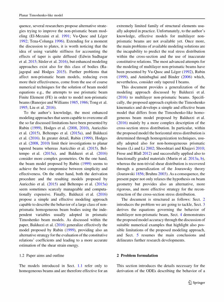
Figure 1 represents the domain X, the adopted
Cartesian coordinate system Oxy, the layer interfaces
y ¼ hi xð Þ for i ¼ 1. . .n þ 1, the beam layers Xj for
j ¼ 1. . .n, and the beam centerline c xð Þ (see Eq. 14).
2.2 2D elastic problem
Being oX the domain boundary—such that
oX :¼ A 0ð Þ [ A lð Þ [ h1 xð Þ [ hnþ1 xð Þ—, we introduce
the partition oXs; oXtf g, where oXs and oXt are the
displacement constrained and the loaded boundaries,
respectively. As usual in beam-model formulation, we
assume that the lower and upper limits belong to the
loaded boundary (i.e., h1 xð Þ and hnþ1 xð Þ 2 oXt)
whereas the initial and final sections A 0ð Þ and A lð Þmay belong to the displacement constrained boundary
O x
y
l
hn+1 A(x) c(x)
x
hnhn−1
hi h2
h1
En,Gn
En−1,Gn−1Ei,Gi
Ei−1,Gi−1E1,G1Ω1
Ωi−1
Ωi
Ωn−1
Ωn
Fig. 1 2D beam geometry, coordinate system, dimensions and
adopted notations
G. Balduzzi et al.
123
oXs that, anyway, must be a non-empty set. Finally, a
distributed load f : X ! R2 is applied within the
domain, a boundary load t : oXt ! R2 is applied on
the loaded boundary, and a suitable boundary dis-
placement function s : oXs ! R2 is assigned on the
displacement constrained boundary.
Being R2�2s the space of symmetric, second order
tensors, we introduce the stress field r : X ! R2�2s ,
the strain field e : X ! R2�2s , and the displacement
field s : X ! R2. Thereby, the strong formulation of
the 2D elastic problem corresponds to the following
boundary value problem
e ¼ rss in X ð7aÞ
r ¼ D : e in X ð7bÞ
r � rþ f ¼ 0 in X ð7cÞ
r � n ¼ t on oXt ð7dÞ
s ¼ s on oXs ð7eÞ
where the operatorrs �ð Þ provides the symmetric part
of the gradient, r � �ð Þ represents the divergence
operator, �ð Þ : �ð Þ denotes the double dot product, andD is the fourth order tensor that defines the mechanical
behavior of the material. Equation (7a) describes the
2D compatibility, Equation (7b) shows the 2D mate-
rial constitutive relation, and 2D equilibrium is
represented by Equation (7c). Equations (7d) and (7e)
represent the boundary equilibrium and the boundary
compatibility conditions where n is the outward unit
vector, defined on the boundary.
It is important to mention that, since the beam body
X is assumed to have no imperfections (e.g., interlayer
delaminations, cracks), the displacement field s is
assumed to be continuous within the whole domain.
Conversely, since the mechanical properties of the
material are defined as piecewise constant functions
(6), according to the 2D material constitutive relation
(7b), the stress field r is expected to be discontinuous
within the domain. Specifically, the discontinuities of
stress field are expected to correspond to the interlayer
surfaces.
2.3 Inter-layer equilibrium
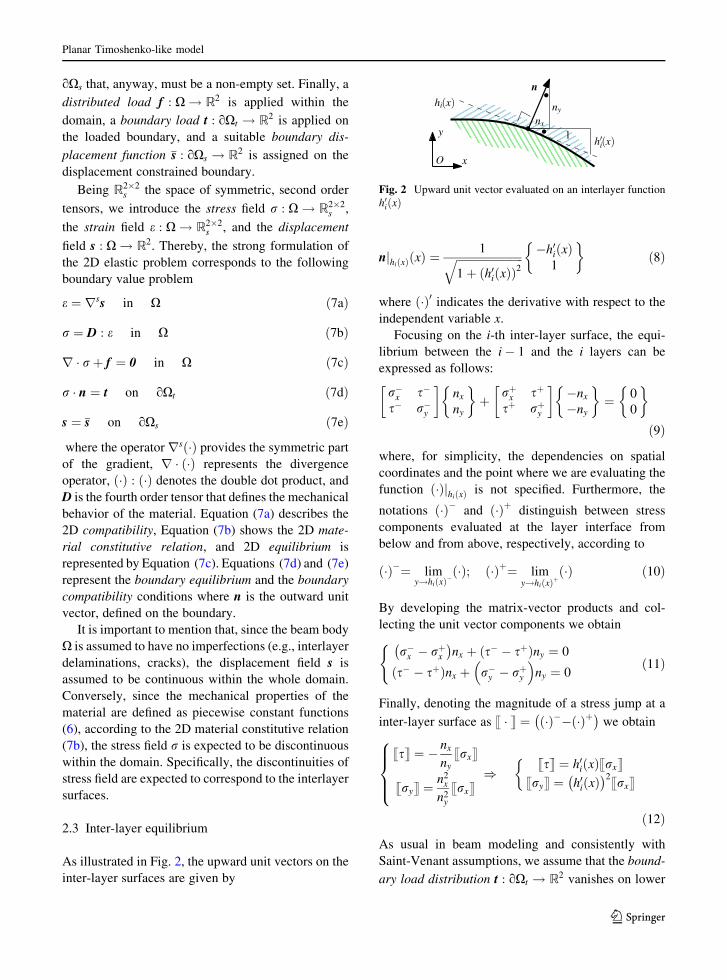
As illustrated in Fig. 2, the upward unit vectors on the
inter-layer surfaces are given by
njhi xð Þ xð Þ ¼ 1ffiffiffiffiffiffiffiffiffiffiffiffiffiffiffiffiffiffiffiffiffiffiffiffi1þ h0
i xð Þð Þ2q �h0
i xð Þ1
� �ð8Þ
where �ð Þ0 indicates the derivative with respect to the
independent variable x.
Focusing on the i-th inter-layer surface, the equi-
librium between the i � 1 and the i layers can be
expressed as follows:
r�x s�
s� r�y
nx
ny
� �þ rþx sþ
sþ rþy
�nx
�ny
� �¼ 0
0
� �
ð9Þ
where, for simplicity, the dependencies on spatial
coordinates and the point where we are evaluating the
function �ð Þjhi xð Þ is not specified. Furthermore, the
notations �ð Þ� and �ð Þþ distinguish between stress
components evaluated at the layer interface from
below and from above, respectively, according to
�ð Þ�¼ limy!hi xð Þ�
�ð Þ; �ð Þþ¼ limy!hi xð Þþ
�ð Þ ð10Þ
By developing the matrix-vector products and col-
lecting the unit vector components we obtain
r�x � rþx� �
nx þ s� � sþð Þny ¼ 0
s� � sþð Þnx þ r�y � rþy
�ny ¼ 0
(
ð11Þ
Finally, denoting the magnitude of a stress jump at a
inter-layer surface as s � t ¼ �ð Þ�� �ð Þþ� �
we obtain
sst ¼ � nx
ny
srxt
sryt ¼n2
x
n2y
srxt
8>><
>>:)
sst ¼ h0i xð Þsrxt
sryt ¼ h0i xð Þ
� �2srxt
�
ð12Þ
As usual in beam modeling and consistently with
Saint-Venant assumptions, we assume that the bound-
ary load distribution t : oXt ! R2 vanishes on lower
O x
ynx
ny
n
1
hi(x)
h′i(x)
Fig. 2 Upward unit vector evaluated on an interlayer function
h0i xð Þ
Planar Timoshenko-like model
123
and upper limits (i.e., tjh1;nþ1¼ 0). Assuming also that
all the stress components vanish outside the beam
domain X, Equation (12) recovers also the stress
constraints coming from boundary equilibrium (7d).
Then, the same relations as described in Auricchio
et al. (2015) and Balduzzi et al. (2016) are obtained.
Considering a multilayer prismatic beam, both
standard and advanced literature states that the hori-
zontal stress has a discontinuous distribution within the
cross-section, in case of different mechanical properties
between the layers, whereas the shear stress has a
continuous distribution (Bareisis 2006; Auricchio et al.
2010; Bardella and Tonelli 2012). In contrary, the inter-
layer equilibrium (12) indicates a discontinuous cross-
section distribution of axial as well as shear stresses.
Furthermore, generalizing the results already discussed
by Auricchio et al. (2015) and Balduzzi et al. (2016),
the horizontal stress rx could be seen as the indepen-
dent variable that completely defines the stress state on
the interlayer surfaces. Finally, generalizing the
results discussed by Boley (1963) and Hodges et al.
(2008, 2010), the shear stress jumps within the cross-
section depend on the variation of the mechanical
properties of the material—determining the jumps of
horizontal stress—and on the slopes of the interlayer
surfaces h0i xð Þ. Therefore the latter seem to be crucial
for the determination of the beam behavior.
3 Simplified 1D model
This section derives the ODEs describing the behavior
of the multilayer non-prismatic beam. The model
consists of 4 main elements:
1. the compatibility equations,
2. the equilibrium equations,
3. the stress representation, and
4. the simplified constitutive relations.
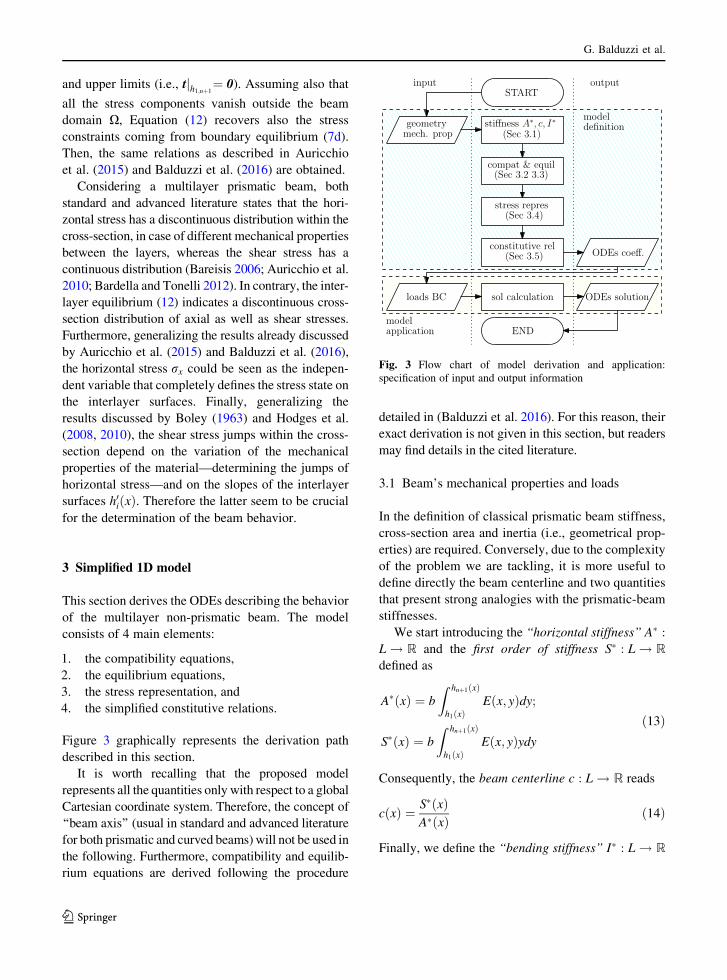
Figure 3 graphically represents the derivation path
described in this section.
It is worth recalling that the proposed model
represents all the quantities only with respect to a global
Cartesian coordinate system. Therefore, the concept of
‘‘beam axis’’ (usual in standard and advanced literature
for both prismatic and curved beams)will not be used in
the following. Furthermore, compatibility and equilib-
rium equations are derived following the procedure
detailed in (Balduzzi et al. 2016). For this reason, their
exact derivation is not given in this section, but readers
may find details in the cited literature.
3.1 Beam’s mechanical properties and loads
In the definition of classical prismatic beam stiffness,
cross-section area and inertia (i.e., geometrical prop-
erties) are required. Conversely, due to the complexity
of the problem we are tackling, it is more useful to
define directly the beam centerline and two quantities
that present strong analogies with the prismatic-beam
stiffnesses.
We start introducing the ‘‘horizontal stiffness’’ A� :L ! R and the first order of stiffness S� : L ! R
defined as
A� xð Þ ¼ b
Z hnþ1 xð Þ
h1 xð ÞE x; yð Þdy;
S� xð Þ ¼ b
Z hnþ1 xð Þ
h1 xð ÞE x; yð Þydy
ð13Þ
Consequently, the beam centerline c : L ! R reads
c xð Þ ¼ S� xð ÞA� xð Þ ð14Þ
Finally, we define the ‘‘bending stiffness’’ I� : L ! R
Fig. 3 Flow chart of model derivation and application:
specification of input and output information
G. Balduzzi et al.
123
I� xð Þ ¼ b
Z hnþ1 xð Þ
h1 xð ÞE yð Þ y � c xð Þð Þ2dy ð15Þ
It is worth recalling that, despite the strong analogy
with prismatic beam coefficients, Definitions (13) and
(15) are not sufficient to define the stiffness of the non-
prismatic beam (see Sect. 3.5). In oder to highlight this
discrepancy, the definition’s names are placed within
quotation marks.
Being fx x; yð Þ and fy x; yð Þ the horizontal and verticalcomponents of the distributed load f , the resulting
loads are defined as
q xð Þ ¼ b
Z hnþ1 xð Þ
h1 xð Þfx x; yð Þdy;
p xð Þ ¼ b
Z hnþ1 xð Þ
h1 xð Þfy x; yð Þdy
m xð Þ ¼ b
Z hnþ1 xð Þ
h1 xð Þfx x; yð Þ c xð Þ � yð Þdy
ð16Þ
where q xð Þ, p xð Þ, and m xð Þ represent the horizontal,
vertical, and bending resulting loads, respectively.
3.2 Compatibility equations
We assume the kinematics usually adopted for pris-
matic Timoshenko beam models. Therefore, the 2D
displacement field s x; yð Þ is represented in terms of
three 1D functions, indicated as generalized displace-
ments: the horizontal displacement u : L ! R, the
rotation u : L ! R, and the vertical displacement
v : L ! R. Specifically, the beam body displacements
are approximated as follows
s x; yð Þ � u xð Þ þ y � c xð Þð Þu xð Þv xð Þ
� �ð17Þ
Furthermore, we introduce the generalized strains i.e.,
the horizontal strain e0 : L ! R, the curvature
v : L ! R, and the shear strain c : L ! R, respec-
tively, which are defined as follows
e0 xð Þ ¼ 1
hnþ1 xð Þ � h1 xð Þ
Z hnþ1 xð Þ
h1 xð Þex x; yð Þdy
v xð Þ ¼ � 12
hnþ1 xð Þ � h1 xð Þð Þ3Z hnþ1 xð Þ
h1 xð Þex x; yð Þ y � c xð Þð Þdy
c xð Þ ¼ 1
hnþ1 xð Þ � h1 xð Þ
Z hnþ1 xð Þ
h1 xð Þexy x; yð Þdy
ð18Þ
where ex and exy are the components of the strain tensor
e.Subsequently, the beam compatibility is expressed
through the following ODEs
e0 xð Þ ¼ u0 xð Þ � c0 xð Þu xð Þ ð19aÞ
v xð Þ ¼ �u0 xð Þ ð19bÞ
c xð Þ ¼ v0 xð Þ þ u xð Þ ð19cÞ
3.3 Equilibrium equations
With the internal forces (i.e., the horizontal internal
force H : L ! R, the vertical internal force
V : L ! R, and the bending moment M : L ! R,
respectively) defined as
H xð Þ ¼ b
Z hnþ1 xð Þ
h1 xð Þrx x; yð Þdy
V xð Þ ¼ b
Z hnþ1 xð Þ
h1 xð Þs x; yð Þdy
M xð Þ ¼ b
Z hnþ1 xð Þ
h1 xð Þrx x; yð Þ c xð Þ � yð Þdy
ð20Þ
the equilibrium ODEs read
H0 xð Þ ¼ �q xð Þ ð21aÞ
M0 xð Þ � H xð Þ � c0 xð Þ þ V xð Þ ¼ �m xð Þ ð21bÞ
V 0 xð Þ ¼ �p xð Þ ð21cÞ
3.4 Stress representation
The representation of stress distributions needs several
definitions. We start by introducing the horizontal-
stress distribution functions dHr : A xð Þ ! R and
dMr : A xð Þ ! R, which define the horizontal stress
distributions induced by horizontal forces and bending
moments, respectively,
dHr x; yð Þ ¼ E x; yð Þ
A� xð Þ ; dMr x; yð Þ ¼ E x; yð Þ
I� xð Þ c xð Þ � yð Þ
ð22Þ
Exploiting Definitions (22), the horizontal stress
distribution can be defined as follows
Planar Timoshenko-like model
123
rx x; yð Þ ¼ dHr x; yð ÞH xð Þ þ dM
r x; yð ÞM xð Þ ð23Þ
Inorder to recover the shear stress distributionwithin the
cross-section we resort to a procedure similar to the one
proposed initially by Jourawski (1856) and nowadays
adopted in most standard literature (Bruhns 2003).
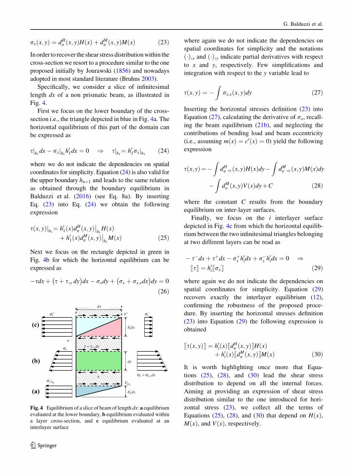
Specifically, we consider a slice of infinitesimal
length dx of a non prismatic beam, as illustrated in
Fig. 4.
First we focus on the lower boundary of the cross-
section i.e., the triangle depicted in blue in Fig. 4a. The
horizontal equilibrium of this part of the domain can
be expressed as
sjh1dx � rxjh1h01dx ¼ 0 ) sjh1¼ h0
1rxjh1 ð24Þ
where we do not indicate the dependencies on spatial
coordinates for simplicity. Equation (24) is also valid for
the upper boundary hnþ1 and leads to the same relation
as obtained through the boundary equilibrium in
Balduzzi et al. (2016) (see Eq. 8a). By inserting
Eq. (23) into Eq. (24) we obtain the following
expression
s x; yð Þjh1¼ h01 xð ÞdH
r x; yð Þ��h1
H xð Þþ h0
1 xð ÞdMr x; yð Þ
��h1
M xð Þ ð25Þ
Next we focus on the rectangle depicted in green in
Fig. 4b for which the horizontal equilibrium can be
expressed as
�sdx þ sþ s;y dy� �
dx � rxdy þ rx þ rx;xdx� �
dy ¼ 0
ð26Þ
where again we do not indicate the dependencies on
spatial coordinates for simplicity and the notations
�ð Þ;x and �ð Þ;y indicate partial derivatives with respect
to x and y, respectively. Few simplifications and
integration with respect to the y variable lead to
s x; yð Þ ¼ �Z
rx;x x; yð Þdy ð27Þ
Inserting the horizontal stresses definition (23) into
Equation (27), calculating the derivative of rx, recall-
ing the beam equilibrium (21b), and neglecting the
contributions of bending load and beam eccentricity
(i.e., assuming m xð Þ ¼ c0 xð Þ ¼ 0) yield the following
expression
s x;yð Þ¼�Z
dHr ;x x;yð ÞH xð Þdy�
ZdMr ;x x;yð ÞM xð Þdy
�Z
dMr x;yð ÞV xð ÞdyþC ð28Þ
where the constant C results from the boundary
equilibrium on inter-layer surfaces.
Finally, we focus on the i interlayer surface
depicted in Fig. 4c from which the horizontal equilib-
rium between the two infinitesimal triangles belonging
at two different layers can be read as
� s�dx þ sþdx � rþx h0idx þ r�x h0
idx ¼ 0 )sst ¼ h0
isrxt ð29Þ
where again we do not indicate the dependencies on
spatial coordinates for simplicity. Equation (29)
recovers exactly the interlayer equilibrium (12),
confirming the robustness of the proposed proce-
dure. By inserting the horizontal stresses definition
(23) into Equation (29) the following expression is
obtained
ss x; yð Þt ¼ h0i xð ÞsdH
r x; yð ÞtH xð Þþ h0
i xð ÞsdMr x; yð ÞtM xð Þ ð30Þ
It is worth highlighting once more that Equa-
tions (25), (28), and (30) lead the shear stress
distribution to depend on all the internal forces.
Aiming at providing an expression of shear stress
distribution similar to the one introduced for hori-
zontal stress (23), we collect all the terms of
Equations (25), (28), and (30) that depend on H xð Þ,M xð Þ, and V xð Þ, respectively.
dx
h′idx
h′1dx
dy
(a)
(b)
(c)
σx|h1 τ |h1τ
τ + τ ,y dyσx
σx +σx,xdx
τ−
τ+σ+x σ−
x
Fig. 4 Equilibrium of a slice of beam of length dx: a equilibriumevaluated at the lower boundary, b equilibrium evaluated within
a layer cross-section, and c equilibrium evaluated at an
interlayer surface
G. Balduzzi et al.
123

Than, the shear-stress distribution dVs : A xð Þ ! R,
defining the shear stress distributions induced by
vertical internal force V xð Þ, can be identified as
dVs x; yð Þ ¼ �
Z y
h1 xð ÞdMr x; tð Þ dt ð31Þ
It is worth mentioning that the so far introduced
definition of shear stress distribution corresponds to
the one provided by Bareisis (2006).
In order to define the shear-stress distributions dHs :
A xð Þ ! R and dMs : A xð Þ ! R induced by horizontal
internal force H xð Þ and bending moment M xð Þrespectively, some additional tools are required. We
start introducing a vector field D : A xð Þ ! Rnþ1. Each
term Di of the vector D is defined as
Di x; yð Þ ¼ d y � hi xð Þð Þh0i xð Þ ð32Þ
where the notation d y � hi xð Þð Þ indicates a Dirac
distribution. Analogously, we define the vectors RH :
L ! Rnþ1 and RM : L ! Rnþ1 as follows
RHi xð Þ ¼ sdH
r x; yð Þt��y¼hi xð Þ; RM
i xð Þ ¼ sdMr x; yð Þt
��y¼hi xð Þ
ð33Þ
Therefore, we define the functions ~dHs ;
~dMs : A xð Þ ! R
~dHs x; yð Þ ¼
Z y
h1 xð ÞD x; tð Þ � RH xð Þ � dH
r ;x x; tð ÞÞ� �
dt
~dMs x; yð Þ ¼
Z y
h1 xð ÞD x; tð Þ � RM xð Þ � dM
r ;x x; tð Þ� �
dt
ð34Þ
and their resulting area
DHs xð Þ ¼
Z hnþ1 xð Þ
h1 xð Þ~dHs x; yð Þdy
DMs xð Þ ¼
Z hnþ1 xð Þ
h1 xð Þ~dMs x; yð Þdy
ð35Þ
As a consequence, the shear-stress distribution func-
tions dHs and dM
s , defining the shear stress distributions
induced by horizontal forceH xð Þ and bendingmoment
M xð Þ, read
dHs x; yð Þ ¼ ~dH
s x; yð Þ � DHs xð ÞdV
s x; yð ÞdMs x; yð Þ ¼ ~dM
s x; yð Þ � DMs xð ÞdV
s x; yð Þð36Þ
According to all so far introduced definitions, the shear
stress distribution can be defined as follows
s x; yð Þ ¼ dHs x; yð ÞH xð Þ þ dM
s x; yð ÞM xð Þ þ dVs yð ÞV xð Þ
ð37Þ
The following statements summarize the key aspects
of the proposed formulation.
• Equations (25), (28), and (30) allow to take into
account the dependency of the shear distribution
within the cross-sections on all the internal forces
H xð Þ, M xð Þ, and V xð Þ.• Furthermore, also the shear stress s exhibits a
discontinuous distribution within the cross-sec-
tion, confirming that a non-prismatic beam
behaves differently from prismatic ones and
according to inter-layer equilibrium discussed in
Sect. 2.3.
• Definitions (31) and (36) satisfy boundary, inter-
nal, and interlayer equilibriums ((25), (28), and
(30), respectively).
• Definition (36) does not ensure that the equilib-
rium on the upper boundary hnþ1 is satisfied. In
particular, it does not guarantee that
limy!hnþ1 xð Þ�
dHs x; yð Þ
�� �� ¼ Dnþ1 x; yð ÞRHnþ1 x; yð Þ
�� ��
limy!hnþ1 xð Þ�
dMs x; yð Þ
�� �� ¼ Dnþ1 x; yð ÞRMnþ1 x; yð Þ
�� ��
ð38Þ
Fortunately, it is possible to proof that Equa-
tion (38) is naturally satisfied since the variation of
the cross-section geometry, inducing the jumps,
compensates with the variation of stress
magnitudes.
• Definition (36) leads
Z hnþ1 xð Þ
h1 xð ÞdHs x; yð Þdy ¼
Z hnþ1 xð Þ
h1 xð ÞdMs x; yð Þdy ¼ 0
ð39Þ
As a consequence, only the shear-stress distribu-
tion functions dVs x; yð Þ depends on the vertical
force V xð Þ, leading to a simpler stress
representation
• Considering an homogeneous beam, the stress
representation provided within this section lead to
the same result as the recovery procedure proposed
in (Balduzzi et al. (2016), Section 3.3). Neverthe-
less, with respect to this reference, the recovery
procedure proposed within this document follows
a more rigorous path.
Planar Timoshenko-like model
123

3.5 Simplified constitutive relations
To complete the Timoshenko-like beam model we
introduce some simplified constitutive relations that
define the generalized strains as a function of the
internal forces.
Therefore, we consider the stress potential, defined
as follows
W� x; yð Þ ¼ 1
2
r2x x; yð ÞE x; yð Þ þ s2 x; yð Þ
G x; yð Þ
� �ð40Þ
Substituting the stress recovery relations (23) and (37)
in Equation (40), the generalized strains result as the
derivatives of the stress potential with respect to the
corresponding internal forces, reading
e0 xð Þ ¼b
Z hnþ1 xð Þ
h1 xð Þ
oW� x; yð ÞoH xð Þ dy ¼
eH xð ÞH xð Þ þ eM xð ÞM xð Þ þ eV xð ÞV xð Þð41aÞ
v xð Þ ¼b
Z hnþ1 xð Þ
h1 xð Þ
oW� x; yð ÞoM xð Þ dy ¼
vH xð ÞH xð Þ þ vM xð ÞM xð Þ þ vV xð ÞV xð Þð41bÞ
c xð Þ ¼b
Z hnþ1 xð Þ
h1 xð Þ
oW� x; yð ÞoV xð Þ dy ¼
cH xð ÞH xð Þ þ cM xð ÞM xð Þ þ cV xð ÞV xð Þð41cÞ
where
eH xð Þ ¼ b
Z hnþ1 xð Þ
h1 xð Þ
dHr x; yð Þ
� �2
E x; yð Þ þdHs x; yð Þ
� �2
G x; yð Þ
!
dy
eM xð Þ ¼ vH xð Þ ¼ b
Z hnþ1 xð Þ
h1 xð Þ
dHr x; yð ÞdM
r x; yð ÞE x; yð Þ dy
þ b
Z hnþ1 xð Þ
h1 xð Þ
dHs x; yð ÞdM
s x; yð ÞG x; yð Þ dy
eV xð Þ ¼ cH xð Þ ¼ b
Z hnþ1 xð Þ
h1 xð Þ
dHs x; yð ÞdM
s x; yð ÞG x; yð Þ dy
vM xð Þ ¼ b
Z hnþ1 xð Þ
h1 xð Þ
dMr x; yð Þ
� �2
E x; yð Þ þdMs x; yð Þ
� �2
G x; yð Þ
!
dy
vV xð Þ ¼ cM xð Þ ¼ b
Z hnþ1 xð Þ
h1 xð Þ
dMs x; yð ÞdV
s x; yð ÞG x; yð Þ dy
cV xð Þ ¼ b
Z hnþ1 xð Þ
h1 xð Þ
dVs x; yð Þ
� �2
G x; yð Þ dy
Equation (41) highlights that curvature and shear
strains depend on both bending moment and vertical
internal force through a non-trivial relation, substan-
tially different from the one that governs the prismatic
beam. This aspect was grasped by Romano (1996) and
was treated more rigorously by Rubin (1999) and
Aminbaghai and Binder (2006) even if their model
uses different coefficients within the constitutive
relations, leading to a coarse estimation of the shear
deformation energy. Furthermore, Equation (41) also
highlights that horizontal and bending stiffnesses non
only depend on the Young’s modulus E, but also on the
shear modulus G.
3.6 Remarks on beam model’s ODEs
Following the notation adopted by Gimena et al.
(2008) the beam model’s ODEs (19), (21), and (41)
can be expressed as
ð42Þ
• The resulting ODEs have the same structure as the
ones obtained by Balduzzi et al. (2016), but differ
due to a more complex definitions of both the
centerline c xð Þ and the constitutive relations.
• Furthermore, the matrix that collects equations’
coefficients has a lower triangular form with
vanishing diagonal terms. As a consequence, the
analytical solution can be easily obtained through
an iterative process of integration done row by
row, starting from H xð Þ and arriving at u xð Þ.• The extremely simple assumptions on kinematics
(17) and internal forces (20) do not allow to tackle
any boundary effect (as usual for most standard
beam models). Therefore the proposed beam
model has not the capability to describe the
phenomena that occurs in the neighborhood of
constraints, concentrated loads, non-smooth
changes of the beam geometry.
G. Balduzzi et al.
123
• Considering a beam made of a single homoge-
neous layer, the herein proposed model recovers
exactly the equations derived by Balduzzi et al.
(2016). Nevertheless, Balduzzi et al. (2016)
recover the shear stress distributions by means of
a suitable (but arbitrary) interpolation of the shear
evaluated at the boundary. On the contrary, the
stress representation provided by Sect. 3.4 rigor-
ously justifies the shear-stress distribution within
the cross-section on the basis of a solid theoretical
background.
• The beam compatibility (19) can be recovered
substituting displacement representation (17) in
2D compatibility (7a) and than inserting the
obtained strains in Equation (18).
• Similarly, the beam equilibrium (21) can be
recovered substituting stress representation (23)
and (37) in 2D equilibrium (7c) and than inserting
the obtained stresses in Equation (20).
For further comments on the resulting ODEs, readers
may refer to Balduzzi et al. (2016).
4 Numerical examples
This section aims at providing further details on the
obtained model capabilities. In particular we consider
three examples: (i) a prismatic cantilever under shear
load, (ii) a non homogeneous tapered beam under
shear load, and (iii) an arch shaped beam under
complex load.
In the following subsections, the stress distributions
will be given with respect to the dimensionless
coordinate y� defined as
y� ¼ y
hnþ1 xð Þ � h1 xð Þð Þjx¼xi
ð43Þ
4.1 Prismatic homogeneous beam
The numerical example provided in this section will
demonstrate that the proposed modeling approach has
the capability to recover the solution of simpler
problems which represents a necessary condition for
proofing the model effectiveness.
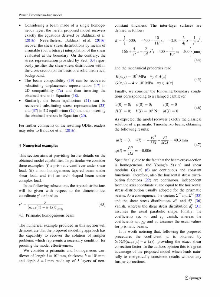
We consider a prismatic and homogeneous can-
tilever of length l ¼ 104 mm, thickness h ¼ 103 mm,
and depth b ¼ 1mm made up of 5 layers of non-
constant thickness. The inter-layer surfaces are
defined as follows
h ¼ �500; �400� 10
11lx; �250� 3
4lx þ 1
l2x2;
�
166þ 5
8lx � 2
3l2x2; 400� 1
10lx; 500
�ðmmÞ
ð44Þ
and the mechanical properties read
E x; yð Þ ¼ 105 MPa 8y 2 A xð ÞG x; yð Þ ¼ 4� 104 MPa 8y 2 A xð Þ
ð45Þ
Finally, we consider the following boundary condi-
tions corresponding to a clamped cantilever
u 0ð Þ ¼ 0; u 0ð Þ ¼ 0; v 0ð Þ ¼ 0
H lð Þ ¼ 0; V lð Þ ¼ 103 N; M lð Þ ¼ 0ð46Þ
As expected, the model recovers exactly the classical
solution of a prismatic Timoshenko beam, obtaining
the following results:
u lð Þ ¼ 0; v lð Þ ¼ � Pl3
3EI� Fl
kGA¼ 40:3mm
u lð Þ ¼ Pl2
2EI¼ �0:006
ð47Þ
Specifically, due to the fact that the beam cross-section
is homogeneous, the Young’s E x; yð Þ and shear
modulus G x; yð Þ (6) are continuous and constant
functions. Therefore, also the horizontal stress distri-
bution functions (22) are continuous, independent
from the axis coordinate x, and equal to the horizontal
stress distribution usually adopted for the prismatic
beams. As a consequence, the vectors RH and RM (33)
and the shear stress distributions dHs and dM
s (36)
vanish, whereas the shear stress distribution dVs (31)
assumes the usual parabolic shape. Finally, the
coefficients eM , eV , and vV vanish, whereas the
coefficients eH , vM and cV assumes the usual values
for prismatic beams.
It is worth noticing that, following the proposed
procedure, the coefficient cV is obtained by
6=5Gb hnþ1 xð Þ � h1 xð Þð Þ, providing the exact shear
correction factor. In the authors opinion this is a great
advantage of the proposed model which leads natu-
rally to energetically consistent results without any
further corrections.
Planar Timoshenko-like model
123
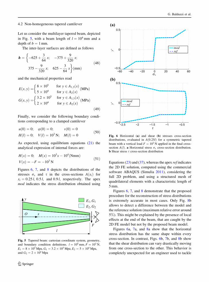
4.2 Non-homogeneous tapered cantilever
Let us consider the multilayer tapered beam, depicted
in Fig. 5, with a beam length of l ¼ 104 mm and a
depth of b ¼ 1mm.
The inter-layer surfaces are defined as follows
h ¼ �625þ 3
64x; �375þ 9
320x;
�
375� 9
320x; 625� 3
64x
�ðmmÞ
ð48Þ
and the mechanical properties read
E x; yð Þ ¼ 8� 105 for y 2 A1;3 xð Þ5� 104 for y 2 A2 xð Þ
�ðMPaÞ
G x; yð Þ ¼ 3:2� 105 for y 2 A1;3 xð Þ2� 104 for y 2 A2 xð Þ
�ðMPaÞ
ð49Þ
Finally, we consider the following boundary condi-
tions corresponding to a clamped cantilever
u 0ð Þ ¼ 0; u 0ð Þ ¼ 0; v 0ð Þ ¼ 0
H lð Þ ¼ 0; V lð Þ ¼ 103 N; M lð Þ ¼ 0ð50Þ
As expected, using equilibrium equations (21) the
analytical expression of internal forces are:
H xð Þ ¼ 0; M xð Þ ¼ 103x � 104ðNmmÞV xð Þ ¼ �F ¼ �103 N
ð51Þ
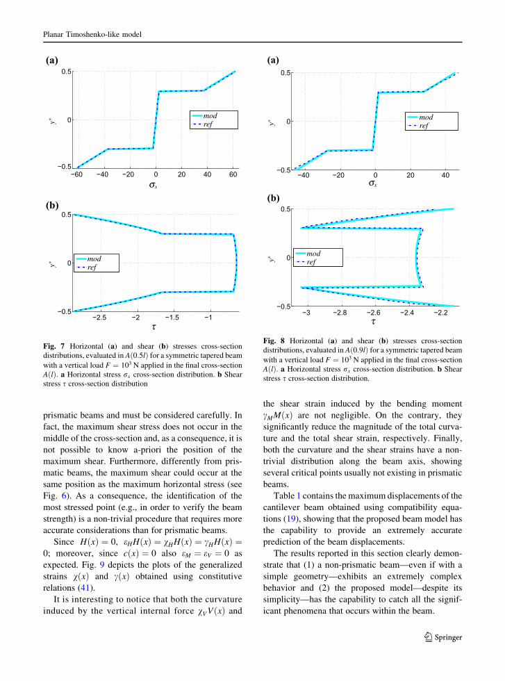
Figures 6, 7, and 8 depicts the distributions of the
stresses rx and s in the cross-sections A xið Þ for
xi ¼ 0:25 l, 0:5 l, and 0:9 l, respectively. The apex
mod indicates the stress distribution obtained using
Equations (23) and (37), whereas the apex ref indicates
the 2D FE solution, computed using the commercial
software ABAQUS (Simulia 2011), considering the
full 2D problem, and using a structured mesh of
quadrilateral elements with a characteristic length of
5mm.
Figures 6, 7, and 8 demonstrate that the proposed
procedure for the reconstruction of stress distributions
is extremely accurate in most cases. Only Fig. 8b
allows to detect a difference between the model and
the reference solution (maximum relative error around
5%). This might be explained by the presence of local
effects at the end of the beam, that are caught by the
2D FE model but not by the proposed beam model.
Figures 6a, 7a, and 8a show that the horizontal
stress distribution has the same shape within every
cross-section. In contrast, Figs. 6b, 7b, and 8b show
that the shear distribution can vary drastically moving
from one cross-section to the other. This behavior is
completely unexpected for an engineer used to tackle
O x
y E1,G1
E2,G2
l
F
Fig. 5 Tapered beam: cartesian coordinate system, geometry,
and boundary condition definitions. l ¼ 104 mm;F ¼ 103 N;
E1 ¼ 8� 105 Mpa;G1 ¼ 3:2� 105 Mpa;E2 ¼ 5� 104 Mpa,
and G2 ¼ 2� 104 Mpa
−60 −40 −20 0 20 40 60−0.5
0
0.5
y∗
modref
σx
−2.5 −2 −1.5 −1 −0.5−0.5
0
0.5
y∗
modref
τ
(a)
(b)
Fig. 6 Horizontal (a) and shear (b) stresses cross-section
distributions, evaluated in A 0:25lð Þ for a symmetric tapered
beam with a vertical load F ¼ 103 N applied in the final cross-
section A lð Þ. a Horizontal stress rx cross-section distribution.
b Shear stress s cross-section distribution
G. Balduzzi et al.
123
prismatic beams and must be considered carefully. In
fact, the maximum shear stress does not occur in the
middle of the cross-section and, as a consequence, it is
not possible to know a-priori the position of the
maximum shear. Furthermore, differently from pris-
matic beams, the maximum shear could occur at the
same position as the maximum horizontal stress (see
Fig. 6). As a consequence, the identification of the
most stressed point (e.g., in order to verify the beam
strength) is a non-trivial procedure that requires more
accurate considerations than for prismatic beams.
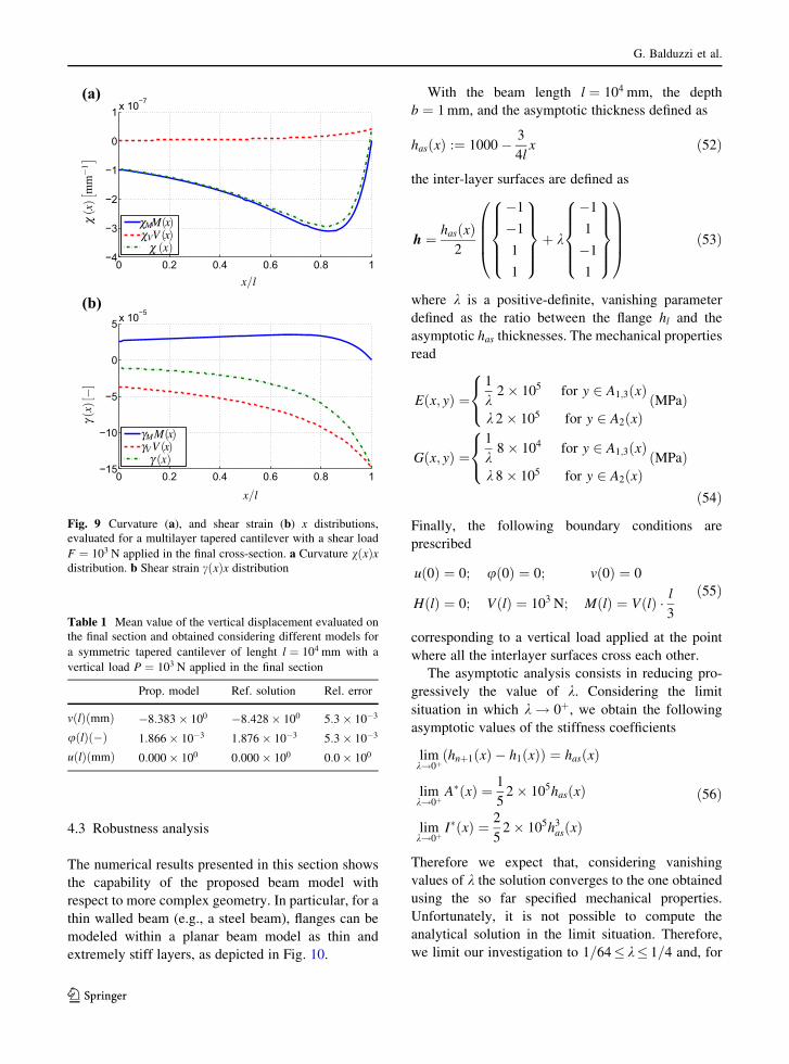
Since H xð Þ ¼ 0, eHH xð Þ ¼ vHH xð Þ ¼ cHH xð Þ ¼0; moreover, since c xð Þ ¼ 0 also eM ¼ eV ¼ 0 as
expected. Fig. 9 depicts the plots of the generalized
strains v xð Þ and c xð Þ obtained using constitutive
relations (41).
It is interesting to notice that both the curvature
induced by the vertical internal force vVV xð Þ and
the shear strain induced by the bending moment
cMM xð Þ are not negligible. On the contrary, they
significantly reduce the magnitude of the total curva-
ture and the total shear strain, respectively. Finally,
both the curvature and the shear strains have a non-
trivial distribution along the beam axis, showing
several critical points usually not existing in prismatic
beams.
Table 1 contains the maximum displacements of the
cantilever beam obtained using compatibility equa-
tions (19), showing that the proposed beam model has
the capability to provide an extremely accurate
prediction of the beam displacements.
The results reported in this section clearly demon-
strate that (1) a non-prismatic beam—even if with a
simple geometry—exhibits an extremely complex
behavior and (2) the proposed model—despite its
simplicity—has the capability to catch all the signif-
icant phenomena that occurs within the beam.
−60 −40 −20 0 20 40 60−0.5
0
0.5
y∗
modref
σx
−2.5 −2 −1.5 −1−0.5
0
0.5
y∗
modref
τ
(a)
(b)
Fig. 7 Horizontal (a) and shear (b) stresses cross-section
distributions, evaluated in A 0:5lð Þ for a symmetric tapered beam
with a vertical load F ¼ 103 N applied in the final cross-section
A lð Þ. a Horizontal stress rx cross-section distribution. b Shear
stress s cross-section distribution
−40 −20 0 20 40−0.5
0
0.5
y∗
modref
σx
−3 −2.8 −2.6 −2.4 −2.2−0.5
0
0.5
y∗
modref
τ
(a)
(b)
Fig. 8 Horizontal (a) and shear (b) stresses cross-section
distributions, evaluated in A 0:9lð Þ for a symmetric tapered beam
with a vertical load F ¼ 103 N applied in the final cross-section
A lð Þ. a Horizontal stress rx cross-section distribution. b Shear
stress s cross-section distribution.
Planar Timoshenko-like model
123
4.3 Robustness analysis
The numerical results presented in this section shows
the capability of the proposed beam model with
respect to more complex geometry. In particular, for a
thin walled beam (e.g., a steel beam), flanges can be
modeled within a planar beam model as thin and
extremely stiff layers, as depicted in Fig. 10.
With the beam length l ¼ 104 mm, the depth
b ¼ 1mm, and the asymptotic thickness defined as
has xð Þ :¼ 1000� 3
4lx ð52Þ
the inter-layer surfaces are defined as
h ¼ has xð Þ2
�1
�1
1
1
8>>><
>>>:
9>>>=
>>>;
þ k
�1
1
�1
1
8>>><
>>>:
9>>>=
>>>;
0
BBB@
1
CCCAð53Þ
where k is a positive-definite, vanishing parameter
defined as the ratio between the flange hl and the
asymptotic has thicknesses. The mechanical properties
read
E x; yð Þ ¼1
k2� 105 for y 2 A1;3 xð Þ
k 2� 105 for y 2 A2 xð Þ
8<
:ðMPaÞ
G x; yð Þ ¼1
k8� 104 for y 2 A1;3 xð Þ
k 8� 105 for y 2 A2 xð Þ
8<
:ðMPaÞ
ð54Þ
Finally, the following boundary conditions are
prescribed
u 0ð Þ ¼ 0; u 0ð Þ ¼ 0; v 0ð Þ ¼ 0
H lð Þ ¼ 0; V lð Þ ¼ 103 N; M lð Þ ¼ V lð Þ � l
3
ð55Þ
corresponding to a vertical load applied at the point
where all the interlayer surfaces cross each other.
The asymptotic analysis consists in reducing pro-
gressively the value of k. Considering the limit
situation in which k ! 0þ, we obtain the following
asymptotic values of the stiffness coefficients
limk!0þ
hnþ1 xð Þ � h1 xð Þð Þ ¼ has xð Þ
limk!0þ
A� xð Þ ¼ 1
52� 105has xð Þ
limk!0þ
I� xð Þ ¼ 2
52� 105h3
as xð Þ
ð56Þ
Therefore we expect that, considering vanishing
values of k the solution converges to the one obtained
using the so far specified mechanical properties.
Unfortunately, it is not possible to compute the
analytical solution in the limit situation. Therefore,
we limit our investigation to 1=64 k 1=4 and, for
0 0.2 0.4 0.6 0.8 1−4
−3
−2
−1
0
1 x 10⁻⁷χ( x)[ m
m−1
]
x/l
χVV (x)χMM(x)
χ (x)
0 0.2 0.4 0.6 0.8 1−15
−10
−5
0
5 x 10⁻⁵
γ(x )[−
]
x/l
γVV (x)γMM(x)
γ (x)
(a)
(b)
Fig. 9 Curvature (a), and shear strain (b) x distributions,
evaluated for a multilayer tapered cantilever with a shear load
F ¼ 103 N applied in the final cross-section. a Curvature v xð Þxdistribution. b Shear strain c xð Þx distribution
Table 1 Mean value of the vertical displacement evaluated on
the final section and obtained considering different models for
a symmetric tapered cantilever of lenght l ¼ 104 mm with a
vertical load P ¼ 103 N applied in the final section
Prop. model Ref. solution Rel. error
v lð ÞðmmÞ �8:383� 100 �8:428� 100 5:3� 10�3
u lð Þð�Þ 1:866� 10�3 1:876� 10�3 5:3� 10�3
u lð ÞðmmÞ 0:000� 100 0:000� 100 0:0� 100
G. Balduzzi et al.
123

every considered k, the reference solution is computed
using the commercial software ABAQUS (Simulia
2011), considering the full 2D problem and using a
structured mesh of quadrilateral elements with a
characteristic length of 5mm.
Figure 11 shows the relative errors for the rotation
u lð Þ and the vertical displacement v lð Þ evaluated at
x ¼ l.
The relative errors in predicting both rotation and
vertical displacement are smaller than 2% in most
cases, even considering small values of k. As a
consequence, we can conclude that the proposed
model is effective and capable to cover most cases of
practical interest.
4.4 Arch shaped beam
The numerical results reported in this section will show
that the proposed beam model can tackle more general
cases, considering generic loads and boundary conditions.
Therefore, the multilayer arch-shaped beam
depicted in Fig. 12 is considered.
With a beam length l ¼ 104 mm and a depth
b ¼ 1mm, the inter-layer surfaces are defined as
h ¼ 363
2000
1
lx2 � 25;
9
50
1
lx2; 500� x
20;
�
525� x
20; 600
oðmmÞ
ð57Þ
whereas the mechanical properties read
E x; yð Þ ¼4� 107 for y 2 A1;3 xð Þ1:6� 106 for y 2 A2 xð Þ1:2� 107 for y 2 A4 xð Þ
8><
>:ðMPaÞ
G x; yð Þ ¼1:538� 107 for y 2 A1;3 xð Þ6:154� 105 for y 2 A2 xð Þ5:217� 106 for y 2 A4 xð Þ
8><
>:ðMPaÞ
ð58Þ
As a consequence, using Equation (14) the centerline
reads
c xð Þ ¼ 7353x4 þ 6:23� 1011x2 þ 4:5� 1015x � 2:4125� 1019
8� 105 87x2 � 1:3� 106x þ 9:25� 1011ð Þð59Þ
Finally, let us consider a distributed load p ¼�1N=mm and the following boundary conditions
u 0ð Þ ¼ 0; H lð Þ ¼ �5� 103 N
v lð Þ ¼ 0; V 0ð Þ ¼ 0
u 0ð Þ ¼ 0; M lð Þ ¼ H lð Þ h1 lð Þ � c lð Þð Þ ¼ 7:953� 106 Nmm
ð60Þ
where the horizontal force H lð Þ and the bending
moment M lð Þ applied at the end of the beam are
O x
y E1,G1E2,G2
l l/3F
Mhas
hl
Fig. 10 Tapered beam: geometry and boundary condition
definition. h0 ¼ 103 mm; hl ¼ 12k h0; l ¼ 104 mm ;F ¼ 103 N,
and M ¼ F � l3
4 8 16 32 64
10−3
10−2
1/λ
e rel
erel ϕ (l)erel v(l)
Fig. 11 Relative errors evaluated for different values of the
parameter k
O x
y
E1,G1E2,G2E3,G3
l
p
M
H
Fig. 12 Arch shaped beam: reference coordinate system,
geometry, and boundary condition definition. l ¼ 104 mm;N ¼5� 103 N; M ¼ �7:953� 106 Nmm; p ¼ 1N=mm;E1 ¼ 4�107 Mpa;G1 ¼ 1:538� 107 Mpa;E2 ¼ 1:6� 106 Mpa;G2 ¼6:154� 105 Mpa;E3 ¼ 1:2� 107 Mpa;G3 ¼ 5:217� 106 Mpa
Planar Timoshenko-like model
123

equivalent to an horizontal force—represented with a
dotted line in Fig. 12—applied at the lower boundary
of the final cross-section.
The distribution of internal forces along the
beam axis, calculated using beam equilibrium
(21), are reported in Fig. 13. Figure 13a clearly
illustrates that the internal forces have the
expected distribution i.e., a constant horizontal
internal force H xð Þ, equal to the load applied in the
final cross-section and a linear distribution of the
vertical internal force V xð Þ. Conversely, Fig. 13b
show that the bending moment M xð Þ is the sum of two
contributions: the formerR
H xð Þ � c0 xð Þdx accounts for
the boundary condition M lð Þ and the moment induced
by the horizontal load due to the variation of the
center-line position within the beam and the latterRV xð Þdx accounts for the bendingmoment induced by
the vertical load p.
Figures 14, 15, and 16 depict the distributions of
the stresses rx and s in the cross-sections A xið Þ wherexi ¼ 0:25 l; 0:5 l; and 0:75 l respectively obtained
using Eqs. (23) and (37). The apex mod indicates the
stress distribution obtained using Equations (23) and
(37), whereas the apex ref indicates the 2D FE
solution, computed using the commercial software
ABAQUS (Simulia 2011), considering the full 2D
problem, and using a structured mesh of quadrilateral
elements with a characteristic length of 5mm.
Figures 14, 15, and 16 demonstrate that the
proposed procedure for the reconstruction of stress
distribution is extremely accurate in most cases. In
particular, Figs. 6b, 7b, and 8b show that the shear
stress distributions vanish at y ¼ h5 xð Þ, confirming
observations reported in Sect. 3.4 and the goodness of
the proposed stress representation procedure. Only
0 0.2 0.4 0.6 0.8 1−5000
0
5000
10000
x/l
Res.Force[N]
H (x)V (x)
0 0.2 0.4 0.6 0.8 1−1
0
1
2
3
4
5x 10⁷
x/l
M(x)[Nmm]
∫H(x)·c′(x)∫V (x)
M (x)
(a)
(b)
Fig. 13 x distribution of internal forces for an arch shaped beam
under complex load condition. a Horizontal H xð Þ and vertical
V xð Þ internal forces x distribution. b Bending moment M xð Þxdistribution
−500 0 500 1000 1500−0.5
0
0.5
y∗
modref
σx
−150 −100 −50 0−0.5
0
0.5
y∗
modref
τ
(a)
(b)
Fig. 14 Horizontal (Fig. 6a) and shear (Fig. 6b) stresses cross-
section distributions, evaluated in A 0:25lð Þ for an arch shaped
beam under complex load condition. a Horizontal stress rx
cross-section distribution. b Shear stress s cross-section
distribution
G. Balduzzi et al.
123
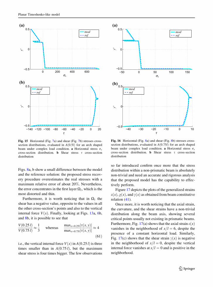
Figs. 8a, b show a small difference between the model
and the reference solution: the proposed stress recov-
ery procedure overestimates the real stresses with a
maximum relative error of about 20%. Nevertheless,
the error concentrates in the first layerX1, which is the
most distorted and thin.
Furthermore, it is worth noticing that in X1 the
shear has a negative value, opposite to the values in all
the other cross-section’s points and also to the vertical
internal force V xð Þ. Finally, looking at Figs. 13a, 6b,
and 8b, it is possible to see that
V 0:25 lð ÞV 0:75 lð Þ �
1
3whereas
maxx¼0:25l s x; yð Þj jmaxx¼0:75l s x; yð Þj j � 4
ð61Þ
i.e., the vertical internal force V xð Þ in A 0:25 lð Þ is threetimes smaller than in A 0:75 lð Þ, but the maximum
shear stress is four times bigger. The few observations
so far introduced confirm once more that the stress
distribution within a non-prismatic beam is absolutely
non-trivial and need an accurate and rigorous analysis
that the proposed model has the capability to effec-
tively perform.
Figure 17 depicts the plots of the generalized strains
e xð Þ, v xð Þ, and c xð Þ as obtained from beam constitutive
relation (41).
Once more, it is worth noticing that the axial strain,
the curvature, and the shear strains have a non-trivial
distribution along the beam axis, showing several
critical points usually not existing in prismatic beams.
Furthermore, Fig. 17(a) shows that the axial strain e xð Þvanishes in the neighborhood of x=l ¼ 6, despite the
presence of a constant horizontal load. Similarly,
Fig. 17(c) shows that the shear strain c xð Þ is negativein the neighborhood of x=l ¼ 0, despite the vertical
internal force vanishes at x=l ¼ 0 and is positive in the
neighborhood.
0 200 400 600−0.5
0
0.5
y∗
modref
σx
−140 −120 −100 −80 −60 −40 −20 0 20−0.5
0
0.5
y∗
modref
τ
(a)
(b)
Fig. 15 Horizontal (Fig. 7a) and shear (Fig. 7b) stresses cross-
section distributions, evaluated in A 0:5lð Þ for an arch shaped
beam under complex load condition. a Horizontal stress rx
cross-section distribution. b Shear stress s cross-section
distribution
−50 0 50 100 150−0.5
0
0.5modref
σx
−40 −30 −20 −10 0 10−0.5
0
0.5
y∗y∗
modref
τ
(a)
(b)
Fig. 16 Horizontal (Fig. 8a) and shear (Fig. 8b) stresses cross-
section distributions, evaluated in A 0:75lð Þ for an arch shaped
beam under complex load condition. a Horizontal stress rx
cross-section distribution. b Shear stress s cross-section
distribution
Planar Timoshenko-like model
123
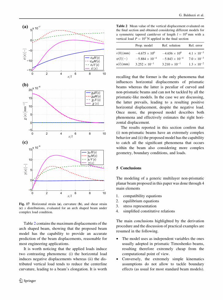
Table 2 contains the maximum displacements of the
arch shaped beam, showing that the proposed beam
model has the capability to provide an accurate
prediction of the beam displacements, reasonable for
most engineering applications.
It is worth noticing that the applied loads induce
two contrasting phenomena: (i) the horizontal load
induces negative displacements whereas (ii) the dis-
tributed vertical load tends to reduce the centerline
curvature, leading to a beam’s elongation. It is worth
recalling that the former is the only phenomena that
influences horizontal displacements of prismatic
beams whereas the latter is peculiar of curved and
non-prismatic beams and can not be tackled by all the
prismatic-like models. In the case we are discussing,
the latter prevails, leading to a resulting positive
horizontal displacement, despite the negative load.
Once more, the proposed model describes both
phenomena and effectively estimates the right hori-
zontal displacement.
The results reported in this section confirm that
(i) non-prismatic beams have an extremely complex
behavior and (ii) the proposedmodel has the capability
to catch all the significant phenomena that occurs
within the beam also considering more complex
geometry, boundary conditions, and loads.
5 Conclusions
The modeling of a generic multilayer non-prismatic
planar beam proposed in this paper was done through 4
main elements
1. compatibility equations
2. equilibrium equations
3. stress representation
4. simplified constitutive relations
The main conclusions highlighted by the derivation
procedure and the discussion of practical examples are
resumed in the following.
• The model uses as independent variables the ones
usually adopted in prismatic Timoshenko beams,
resulting therefore extremely cheap from the
computational point of view.
• Conversely, the extremely simple kinematics
assumptions do not allow to tackle boundary
effects (as usual for most standard beam models).
0 2 4 6 8 10−15
−10
−5
0
5 x 10⁻⁷ε(
x)[−
]
x/l
εHH(x)
εVV (x)εMM(x)
ε (x)
0 2 4 6 8 10−5
0
5
10
15
20 x 10−8
χ(x)[ m
m−1
]
x/l
χVV (x)χMM(x)χHH(x)
χ (x)
0 2 4 6 8 10−5
0
5
10
15 x 10−6
γ(x)[ −
]
x/l
γHH(x)
γVV (x)γMM(x)
γ (x)
(a)
(b)
(c)
Fig. 17 Horizontal strain (a), curvature (b), and shear strain
(c) x distributions, evaluated for an arch shaped beam under
complex load condition.
Table 2 Mean value of the vertical displacement evaluated on
the final section and obtained considering different models for
a symmetric tapered cantilever of length l ¼ 104 mm with a
vertical load P ¼ 103 N applied in the final section
Prop. model Ref. solution Rel. error
v 0ð ÞðmmÞ �4:675� 100 �4:656� 100 4:1� 10�3
u lð Þð�Þ �5:884� 10�4 �5:843� 10�4 7:0� 10�3
u lð ÞðmmÞ 3:252� 10�1 3:210� 10�1 1:3� 10�2
G. Balduzzi et al.
123
Therefore the proposed beam model has not the
capability to describe the phenomena occurring in
the neighborhood of constraints, concentrated
loads, and corners.
• The proposed stress representation highlights that
the shear distribution not only depends on vertical
internal force (as usual fo prismatic beams) but
also on horizontal internal force and bending
moment.
• The complex geometry of multilayer non-pris-
matic beams causes each generalized strain to
depend on all internal forces. The proposed
simplified constitutive relations allow to effec-
tively describe these phenomena, leading to a
consistent and robust beam model.
• The examples discussed in Sect. 4 highlights that
non-prismatic multilayer beams could behave very
differently than prismatic ones.
• Furthermore, numerical examples demonstrate
that the model is effective, robust, and accurate
also for complex geometries (like highly hetero-
geneous beams with extremely thin layers), loads,
and boundary conditions, leading the model to be a
promising tool for practitioners and researcher.
Further developments of the present work will include
the application of the proposed model to more realistic
cases, the consideration of both dynamic and buckling
behaviors, the development of a non-prismatic beam
FE formulation, and the generalization of the proposed
modeling procedure to 3D beams.
Acknowledgements This work was funded by the Austrian
Science Found (FWF): M 2009-N32.
Open Access This article is distributed under the terms of the
Creative Commons Attribution 4.0 International License (http://
creativecommons.org/licenses/by/4.0/), which permits unrest-
ricted use, distribution, and reproduction in any medium, pro-
vided you give appropriate credit to the original author(s) and
the source, provide a link to the Creative Commons license, and
indicate if changes were made.
References
Allaire, G., Bonnetier, E., Francfort, G., Jouve, F.: Shape opti-
mization by the homogenization method. Numerische
Mathematik 76(1), 27–68 (1997)
Aminbaghai, M., Binder, R.: Analytische Berechnung von
Voutenstaben nach Theorie II. Ordnung unter
Berucksichtigung der M- und Q- Verformungen.
Bautechnik 83, 770–776 (2006)
Atkin, E.H.: Tapered beams: suggested solutions for some
typical aircraft cases. Aircr. Eng. 10, 371–374 (1938)
Auricchio, F., Balduzzi, G., Lovadina, C.: A new modeling
approach for planar beams: finite-element solutions based
on mixed variational derivations. J. Mech. Mater. Struct. 5,771–794 (2010)
Auricchio, F., Balduzzi, G., Lovadina, C.: The dimensional
reduction approach for 2D non-prismatic beam modelling:
a solution based on Hellinger–Reissner principle. Int.
J. Solids Struct. 15, 264–276 (2015)
Balduzzi, G., Aminbaghai, M., Sacco, E., Fussl, J., Eberhard-
steiner, J., Auricchio F.: Non-prismatic beams: a simple
and effective Timoshenko-like model. Int. J. Solids Struct.
90, 236–250 (2016)
Banerjee, J.R., Williams, F.W.: Exact Bernoulli–Euler dynamic
stiffness matrix for a range of tapered beams. Int. J. Numer.
Methods Eng. 21(12), 2289–2302 (1985)
Banerjee, J.R., Williams, F.W.: Exact Bernoulli–Euler static
stiffness matrix for a range of tapered beam-columns. Int.
J. Numer. Methods Eng. 23, 1615–1628 (1986)
Bardella, L., Tonelli, D.: Explicit analytic solutions for the
accurate evaluation of the shear stresses in sandwich
beams. J. Eng. Mech. 138, 502–507 (2012)
Bareisis, J.: Stiffness and strength of multilayer beams.
J. Compos. Mater. 40, 515–531 (2006)
Beltempo, A., Balduzzi, G., Alfano, G., Auricchio, F.: Analyt-
ical derivation of a general 2D non-prismatic beam model
based on the Hellinger–Reissner principle. Eng. Struct.
101, 88–98 (2015a)
Beltempo, A., Cappello, C., Zonta, D., Bonelli, A., Bursi, O.,
Costa, C., Pardatscher, W.: Structural health monitoring of
the Colle Isarco viaduct. In: 2015 IEEE Workshop on
Environmental, Energy and Structural Monitoring Systems
(EESMS), pp. 7–11. IEEE (2015b)
Boley, B.A.: On the accuracy of the Bernoulli–Euler theory for
beams of variable section. J. Appl. Mech. 30, 374–378(1963)
Bruhns, O.T.: Advanced Mechanics of Solids. Springer, Berlin
(2003)
Edwin Sudhagar, P., Ananda Babu, A., Rajamohan, V., Jeyaraj,
P.: Structural optimization of rotating tapered laminated
thick composite plates with ply drop-offs. Int. J. Mech.
Mater. Des. 1–40 (2015). doi:10.1007/s10999-015-9319-9
El-Mezaini, N., Balkaya, C., Citipitioglu, E.: Analysis of frames
with nonprismatic members. J. Struct. Eng. 117,1573–1592 (1991)
Frese, M., Blaß, H.J.: Asymmetrically combined glulam aLS
simplified verification of the bending strength. In: CIB-
W18/45-12-1 International Council for Reserach and
Innovation in Builfing and Construction, Working Com-
mission W18—timber structures—Meeting fortyfive
Vaxjo Sweden August 2012 (2012)
Friedman, Z., Kosmatka, J.B.: Exact stiffness matrix of a
nonuniform beam—II bending of a Timoshenko beam.
Comput. Struct. 49(3), 545–555 (1993)
Gimena, L., Gimena, F., Gonzaga, P.: Structural analysis of a
curved beam element defined in global coordinates. Eng.
Struct. 30, 3355–3364 (2008)
Planar Timoshenko-like model
123
Hodges, D.H., Ho, J.C., Yu, W.: The effect of taper on section
constants for in-plane deformation of an isotropic strip.
J. Mech. Mater. Struct. 3, 425–440 (2008)
Hodges, D.H., Rajagopal, A., Ho, J.C., Yu, W.: Stress and strain
recovery for the in-plane deformation of an isotropic
tapered strip-beam. J. Mech. Mater. Struct. 5, 963–975(2010)
Jourawski, D.: Sur le resistance daZun corps prismatique et
daZune piece composee en bois ou on tole de fer a une
force perpendiculaire a leur longeur. In Annales des Ponts
et Chaussees 12, 328–351 (1856)
Lee, E., James, K.A., Martins, J.R.R.A.: Stress-constrained
topology optimization with design-dependent loading.
Struct. Multidiscip. Optim. 46(5), 647–661 (2012)
Li, G.-Q., Li, J.-J.: A tapered Timoshenko–Euler beam element
for analysis of steel portal frames. J. Construct. Steel Res.
58, 1531–1544 (2002)
Liu, S.-W., Bai, R., Chan, S.-L.: Second-order analysis of non-
prismatic steel members by tapered beam-column ele-
ments. Structures 6, 108–118 (2016)
Maganti, N.R., Nalluri, M.R.: Flapwise bending vibration
analysis of functionally graded rotating double-tapered
beams. Int. J. Mech. Mater. Eng. 10(1), 1–10 (2015)
Murin, J., Aminbaghai, M., Hrabovsky, J., Kutis, V., Kugler, S.:
Modal analysis of the FGM beams with effect of the shear
correction function. Compos. Part B Eng. 45(1),1575–1582 (2013a)
Murin, J., Aminbaghai, M., Kutis, V., Hrabovsky, J.: Modal
analysis of the FGM beams with effect of axial force under
longitudinal variable elastic Winkler foundation. Eng.
Struct. 49, 234–247 (2013b)
Paglietti, A., Carta, G.: La favola del taglio efficace nella teoria
delle travi di altezza variabile. In: AIMETA (2007)
Paglietti, A., Carta, G.: Remarks on the current theory of shear
strength of variable depth beams. Open Civil Eng. J. 3,28–33 (2009)
Portland Cement Associations: Portland Cement Associations:
Handbook of Frame Constants. Beam Factor and Moment
Coefficients for Members of Variable Section. Portland
Cement Associations, Washington, DC (1958)
Rajagopal, A., Hodges, D.H.: Variational asymptotic analysis
for plates of variable thickness. Int. J. Solids Struct. 75,81–87 (2015)
Romano, F.: Deflections of Timoshenko beam with varying
cross-section. Int. J. Mech. Sci. 38(8–9), 1017–1035 (1996)Romano, F., Zingone, G.: Deflections of beams with varying
rectangular cross section. J. Eng. Mech. 118(10),2128–2134 (1992)
Rubin, H.: Analytische Berechnung von Staben mit linear
veranderlicher Hohe unter Berucksichtigung von M-, Q-
und N- Verformungen. Stahlbau 68, 112–119 (1999)
Schreyer, H.L.: Elementary theory for linearly tapered beams.
J. Eng. Mech. Div. 104(3), 515–527 (1978)
Shooshtari, A., Khajavi, R.: An efficent procedure to find shape
functions and stiffness matrices of nonprismatic Euler–
Bernoulli and Timoshenko beam elements. Eur. J. Mech.
A/Solids 29, 826–836 (2010)
Simulia: ABAQUS User’s and theory manuals—Release 6.11.
Simulia, Providence (2011)
Susler, S., Turkmen, H.S., Kazancı, Z.: Nonlinear dynamic
analysis of tapered sandwich plates with multi-layered
faces subjected to air blast loading. Int. J. Mech. Mater.
Des. 1–23 (2016). doi:10.1007/s10999-016-9346-1
Tena-Colunga, A.: Stiffness formulation for nonprismatic beam
elements. J. Struct. Eng. 122, 1484–1489 (1996)
Timoshenko, S., Goodier, J.N.: Theory of Elasticity, 2nd edn.
McGraw-Hill, New York City (1951)
Timoshenko, S.P., Young, D.H.: Theory of Structures.
McGraw-Hill, New York City (1965)
Tong, X., Tabarrok, B., Yeh, K.: Vibration analysis of
Timoshenko beams with non-homogeneity and varying
cross-section. J. Sound Vib. 186(5), 821–835 (1995)
Trinh, T.H., Gan, B.S.: Development of consistent shape func-
tions for linearly solid tapered Timoshenko beam. J. Struct.
Construct. Eng. 80, 1103–1111 (2015)
Vu-Quoc, L., Leger, P.: Efficient evaluation of the flexibility of
tapered I-beams accounting for shear deformations. Int.
J. Numer. Methods Eng. 33(3), 553–566 (1992)
G. Balduzzi et al.
123
Top Related