

Languages
Pages
Legal


Essays on Pensions and Savings
Eelco Dirk Zandberg

Publisher: University of Groningen, Groningen, The Netherlands
Printed by: Ipskamp Drukkers
P.O. Box 333
7500 AH Enschede
The Netherlands
ISBN: 978-90-367-8200-5 / 978-90-367-8199-2 (electronic version)
c⃝ 2015 Eelco Zandberg
All rights reserved. No part of this publication may be reproduced, stored in a re-
trieval system of any nature, or transmitted in any form or by any means, electronic,
mechanical, now known or hereafter invented, including photocopying or record-
ing, without prior written permission of the publisher.

Essays on Pensions and Savings
Proefschrift
ter verkrijging van de graad van doctor aan de Rijksuniversiteit Groningen
op gezag van de rector magnificus prof. dr. E. Sterken
en volgens besluit van het College voor Promoties.
De openbare verdediging zal plaatsvinden op
maandag 19 oktober 2015 om 16.15 uur
door
Eelco Dirk Zandberg
geboren op 13 juli 1982 te Haskerland

Promotores
Prof. dr. L. Spierdijk
Prof. dr. R.J.M. Alessie
Beoordelingscommissie
Prof. dr. B.W. Lensink
Prof. dr. A.H.O. van Soest
Prof. dr. A. Barrett

Acknowledgements
When I applied for a PhD position at the Faculty of Economics and Business back
in 2009 I expected to write a thesis about ’monetary policy in a globalizing world’.
Six years later I have finished a thesis about ’pensions and savings’.
First of all, I would like to thank Laura for giving me the opportunity to start
working on a topic that was completely new for me at the time. During my PhD
you kept stimulating me to work on issues that interested me. When I indicated
after a few months that I preferred to change the research topic a little bit, you were
the first to support me.
After two years Rob Alessie became my second supervisor. The rigor with which
you commented on my papers was very welcome and has resulted in a better thesis
in the end. Also, I have appreciated your endless patience and willingness to dis-
cuss issues around household saving patterns.
I would like to thank the PhD coordinators, Martin Land and Linda Toolsema,
and of course the rest of the SOM office for their willingness to assist with all kinds
of administrative duties.
This thesis would not have existed without the financial support of Netspar.
Thank you for giving me the opportunity to work four years on these very interest-
ing issues.
The first two persons who really enthused me for doing research were Jakob de
Haan and Richard Jong-A-Pin. The research-oriented course Political Economics,
which you taught in the spring of 2007, made me decide to apply for the Research
Master and subsequently a PhD position.
Jochen Reiner became one of my best friends after we were study mates during
the Research Master. After the Research Master you started a PhD in Frankfurt,
but we kept visiting each other every few months. And we still talk about doing
research every now and then, despite the fact that you are an assistant professor in
Marketing in the meantime and I am working in the private sector.
I would like to thank my FEB colleagues, in particular Pim, Allard, Remco,
Tomek, Rients, Lammertjan, and Peter. The conversations at the coffee machine

ii
usually had one thing in common: They were neverending and always converged
to discussions about cycling. A special thanks goes to Aljar Meesters. The discus-
sions we had about statistics, econometrics, and science in general were very valu-
able to me. You partly changed my point of view.
Thanks to my current colleagues at TKP Pensioen for taking care of my duties
when I had to take off to work on my thesis. A special thanks goes to my former
boss, Max Pieters, for immediately suggesting me to take two full weeks off when
I indicated that I really needed some time to finish the last chapter of the thesis.
Thanks to my family for always supporting me. A special thanks goes to Dicky
and Madeleine for taking care of our two little boys many, many times. With your
help it became a little bit easier to write a PhD thesis while raising two children.
Finally, the three most important people in my life: I would not have finished
this thesis without you. Thank you for all your support, Suzanne, Julian, and To-
bias. I dedicate this thesis to you.
Eelco Zandberg

Contents
1 Introduction 1
1.1 Introduction . . . . . . . . . . . . . . . . . . . . . . . . . . . . . . . . . 1
1.2 Chapters 2-4 . . . . . . . . . . . . . . . . . . . . . . . . . . . . . . . . . 3
1.2.1 Introduction . . . . . . . . . . . . . . . . . . . . . . . . . . . . . 3
1.2.2 Chapter 2: Research Question, Findings, Conclusions . . . . . 4
1.2.3 Chapter 3: Research Question, Findings, Conclusions . . . . . 5
1.2.4 Chapter 4: Research Question, Findings, Conclusions . . . . . 5
1.3 Chapter 5 . . . . . . . . . . . . . . . . . . . . . . . . . . . . . . . . . . . 7
1.3.1 Introduction . . . . . . . . . . . . . . . . . . . . . . . . . . . . . 7
1.3.2 Chapter 5: Research Question, Findings, Conclusions . . . . . 7
2 Education level and age-wealth profiles 9
2.1 Introduction . . . . . . . . . . . . . . . . . . . . . . . . . . . . . . . . . 9
2.2 Theoretical Considerations . . . . . . . . . . . . . . . . . . . . . . . . . 12
2.2.1 The Dutch Pension System . . . . . . . . . . . . . . . . . . . . 12
2.2.2 Life Cycle Model . . . . . . . . . . . . . . . . . . . . . . . . . . 13
2.3 The Data . . . . . . . . . . . . . . . . . . . . . . . . . . . . . . . . . . . 16
2.4 Econometric Framework . . . . . . . . . . . . . . . . . . . . . . . . . . 22
2.4.1 Empirical Strategy . . . . . . . . . . . . . . . . . . . . . . . . . 22
2.4.2 Permanent Income . . . . . . . . . . . . . . . . . . . . . . . . . 24
2.5 Results . . . . . . . . . . . . . . . . . . . . . . . . . . . . . . . . . . . . 30
2.6 Conclusions . . . . . . . . . . . . . . . . . . . . . . . . . . . . . . . . . 38
2.A Appendix . . . . . . . . . . . . . . . . . . . . . . . . . . . . . . . . . . 39
3 The retirement replacement rate 41
3.1 Introduction . . . . . . . . . . . . . . . . . . . . . . . . . . . . . . . . . 41
3.2 The U.S. Pension System . . . . . . . . . . . . . . . . . . . . . . . . . . 43

iv Contents
3.2.1 First pillar: Social Security . . . . . . . . . . . . . . . . . . . . . 43
3.2.2 Second pillar: Employer-provided pension schemes and 401(k)
plans . . . . . . . . . . . . . . . . . . . . . . . . . . . . . . . . . 45
3.2.3 Third pillar: IRAs and other annuities . . . . . . . . . . . . . . 45
3.3 Calculating Replacement Rates . . . . . . . . . . . . . . . . . . . . . . 46
3.4 Which Variables are Correlated with the Replacement Rate? . . . . . 53
3.5 Conclusions . . . . . . . . . . . . . . . . . . . . . . . . . . . . . . . . . 56
3.A Appendix . . . . . . . . . . . . . . . . . . . . . . . . . . . . . . . . . . 57
4 Retirement replacement rates and saving behavior 61
4.1 Introduction . . . . . . . . . . . . . . . . . . . . . . . . . . . . . . . . . 61
4.2 Data . . . . . . . . . . . . . . . . . . . . . . . . . . . . . . . . . . . . . . 64
4.3 Identification and Empirical Model . . . . . . . . . . . . . . . . . . . . 68
4.4 Results . . . . . . . . . . . . . . . . . . . . . . . . . . . . . . . . . . . . 71
4.4.1 Baseline Specification . . . . . . . . . . . . . . . . . . . . . . . 72
4.4.2 Age-Wealth Profiles . . . . . . . . . . . . . . . . . . . . . . . . 74
4.4.3 Robustness Checks . . . . . . . . . . . . . . . . . . . . . . . . . 77
4.5 Conclusions . . . . . . . . . . . . . . . . . . . . . . . . . . . . . . . . . 88
5 Funding of pensions and economic growth 89
5.1 Introduction . . . . . . . . . . . . . . . . . . . . . . . . . . . . . . . . . 89
5.2 Theory . . . . . . . . . . . . . . . . . . . . . . . . . . . . . . . . . . . . 91
5.2.1 Aggregate Saving Rate . . . . . . . . . . . . . . . . . . . . . . . 91
5.2.2 Other Channels . . . . . . . . . . . . . . . . . . . . . . . . . . . 94
5.3 Data Description . . . . . . . . . . . . . . . . . . . . . . . . . . . . . . 94
5.4 Empirical Results . . . . . . . . . . . . . . . . . . . . . . . . . . . . . . 97
5.4.1 Short-run effects . . . . . . . . . . . . . . . . . . . . . . . . . . 97
5.4.2 Long-run effects . . . . . . . . . . . . . . . . . . . . . . . . . . 100
5.5 Conclusions . . . . . . . . . . . . . . . . . . . . . . . . . . . . . . . . . 105
References 107
Samenvatting (Summary in Dutch) 117

Chapter 1
Introduction
1.1 Introduction
Most Western countries face an aging population. For example, in the Netherlands
the ratio of workers to pensioners will fall from four in 2012 to two in 20401. In other
Western countries, the numbers are comparable. This is caused by two things: First,
the Post-World War II baby boom. This event will have a temporary effect on the
age structure of Western countries. The second cause, increasing life expectancy, is
permanent. Although increasing life expectancy is a joyful thing in itself, it poses
large challenges to health care costs and the economic viability of pension systems.
Several measures have been taken to meet the aging challenge. The legal retire-
ment age has been increased, measures have been taken to increase labor supply
among older workers, and some countries are switching from a pay-as-you-go pen-
sion system to a funded system. All these measures are part of the solution to the
aging problem, but might have other effects as well. For example, Davis and Hu
(2008) claim that funding of pensions spurs economic growth.
A related development is the trend from defined benefit towards defined con-
tribution schemes. An important feature of a defined contribution system is that
individuals (or households) have to absorb investment shocks, interest rate shocks,
and inflation shocks themselves, while in a defined benefit system intergenerational
risk sharing spreads these shocks out over different generations. Therefore, the shift
towards defined contribution can be seen as part of the broader shift towards more
individual responsibility. Saving for retirement becomes more and more an indi-
vidual task, also in the Netherlands.
1 Source: CBS StatLine, http://statline.cbs.nl.

2 Chapter 1
This thesis aims to answer important questions related to aging and saving be-
havior of households: How do retirement replacement rates affect saving behavior
of households? What are the macroeconomic effects when governments decide to
reform the pension system? These two questions are the main focus of attention
of this thesis. To be a bit more specific, this thesis consists of four studies. The first
three studies (Chapters 2, 3, and 4) examine life-cycle saving patterns, while the last
study (Chapter 5) deals with the presumed link between funding of pensions and
economic growth.
The effect of retirement replacement rates on saving behavior is important, be-
cause retirement replacement rates are declining in most Western countries. This
is partly caused by the shift from defined benefit towards defined contribution
schemes. But also defined benefit schemes are becoming less and less generous.
To prevent a steep drop in standard of living after retirement, people thus need to
save in addition to their pension scheme.
Examining life-cycle saving patterns (Chapters 2, 3, and 4) is also motivated
by the observation that out-of-pocket medical expenses hardly exist in the Dutch
health care system, that public pensions are very generous and that the private
pension system is among the best worldwide. So why do people save so much?
Considering it from a life-cycle perspective, the fact that the elderly hardly dissave
already suggests that there is no need for it.
As we noted above, one of the measures that has been taken to confront aging
is funding of pensions. The topic of Chapter 5 is motivated by one of the main
arguments in favor of funding of pensions, namely that funded pension systems are
more resistant to large shocks to the age structure of the population than unfunded
pension systems. However, as Barr (2000) explains, also funded pension systems
are vulnerable to demographic shocks. According to him, the idea that funding
of pensions resolves adverse demographics is one of the ten myths about pension
reform. However, quite some countries are reforming their systems at great costs.
Therefore, we want to examine whether there are macroeconomic effects of these
reforms and whether these effects are positive or negative.
The rest of the introduction is organized as follows: Section 2 describes Chapters
2, 3 and 4 of this thesis. After a short introduction of the topic we will state for each
Chapter its research question, the main findings, and the conclusions. Section 3
offers a short introduction to Chapter 5, of which the theme slightly diverges from
Chapters 2, 3, and 4, again with research question, main findings, and conclusions.

Introduction 3
1.2 Chapters 2-4
1.2.1 Introduction
Since the life-cycle and permanent income hypotheses were posited almost 60 years
ago (Modigliani and Brumberg, 1954, Friedman, 1957) many studies have tested
their implications. One of those is that households, confronted with a hump-shaped
lifetime-income profile, save when they are young and decumulate their savings
after retirement, in order to smooth consumption over the lifetime.
Initially, age-wealth profiles were examined using only discretionary wealth.
The results of these kinds of analyses are mixed (see Browning and Lusardi (1996)).
Most studies simply do not find that households decumulate wealth after retire-
ment and if they do, only at a very slow pace. Several explanations were developed
for the lack of dissaving during retirement. The most important among these are
a precautionary saving motive, uncertainty concerning the time of death and a be-
quest motive.
An alternative explanation is provided by Jappelli and Modigliani (2006). They
argue that mandatory pension premiums are part of saving and, on the other hand,
pension benefits are not part of income that is consumed but wealth decumulation
(see also Auerbach et al. (1991), Gokhale et al. (1996) and Miles (1999), among oth-
ers). According to them, failing to take pension wealth into account would bias the
results of testing the life-cycle hypothesis towards rejecting it. They then show that
adding pension wealth to discretionary wealth produces a perfectly hump-shaped
age-wealth profile for Italian households.
However, this ignores the fact that the design of a mandatory pension system
automatically leads to a hump-shaped age-wealth profile. The decision to accumu-
late wealth through the pension system and decumulate wealth after retirement is
fully beyond the control of households. In that sense it is questionable whether it
constitutes a valid test of the life-cycle model to include pension wealth as it is not
the outcome of a deliberate saving decision by households2. On the other hand, it
is clear that ignoring the pension system and only looking at discretionary wealth
is misleading as well.
Therefore, we propose a test of the life-cycle hypothesis that uses only dis-
cretionary wealth but takes the effects of the pension system on wealth accumu-
lation (and decumulation) into account. In Chapter 2 we do this in an indirect
2 This is not to say that taking pension wealth into account is not important to calculate aggregatesaving rates more accurately.

4 Chapter 1
way using Dutch data. We test whether educational attainment is related to the
amount of wealth that households accumulate before retirement, and decumulate
after retirement. This approach exploits differences in the retirement replacement
rate between groups of Dutch households with different educational attainment.
In Chapters 3 and 4 we use U.S. data. Chapter 3 is mainly descriptive, we discuss
how we calculate retirement replacement rates from the Health and Retirement
Study (HRS) and examine which factors correlate with the retirement replacement
rate. Finally, in Chapter 4 we directly examine the link between retirement replace-
ment rates and saving behavior, using the replacement rates that we calculated in
Chapter 3.
1.2.2 Chapter 2: Research Question, Findings, Conclusions
In Chapter 2, the following research question is dealt with:
Do households with higher educational attainment have steeper age-wealth pro-
files than households with lower educational attainment?
Our contribution to the literature is twofold: First, we take the retirement replace-
ment rate as the basis of our analysis of differences in age-wealth profiles between
groups of households. Second, we use a long panel (1995-2011) with Dutch data
(DNB Household Survey (DHS)), which enables us to observe changes in house-
hold wealth over time. The combination of high data quality and a long panel
makes the DHS very suitable for our purpose. Other datasets are the IPO (Inko-
mens Panel Onderzoek), and the Socio-Economic Panel (SEP), which consists of
administrative data. As Alessie et al. (1997) and Kapteyn et al. (2005) note, stocks,
bonds, and savings accounts are severely underreported in the SEP and the level of
measurement error is not constant over time.
To test some of the implications of the life cycle-permanent income hypothesis
we examine education-specific age-wealth profiles at the household level. Our sam-
ple is an unbalanced panel of 17 years (1994-2010) and approximately 2500 house-
holds of Dutch data. We find that, even after controlling for permanent income,
highly educated households accumulate more non-housing wealth during working
life than low-educated households. Furthermore, only highly educated households
seem to decumulate non-housing wealth after retirement. On the other hand, most
households hardly decumulate housing wealth after retirement.
Especially the finding that the behavior of highly educated households is broadly

Introduction 5
in line with the life-cycle hypothesis, suggests that this group of households would
be able to handle more freedom of choice with respect to saving for retirement in
the Netherlands. Of course, higher financial literacy might have caused the results,
but this is an additional argument for more individual freedom of choice regarding
pensions.
1.2.3 Chapter 3: Research Question, Findings, Conclusions
In Chapter 3, the following research questions are dealt with:
How can the retirement replacement rate of households be calculated from the HRS
data? Which factors correlate with the retirement replacement rate?
The aim of this chapter is mainly descriptive. We show how to calculate replace-
ment rates from the HRS data, describe the main features of our measure, and ex-
amine which factors are correlated with the replacement rate. Two other studies
calculate replacement rates from other data sources: Bernheim et al. (2001) calcu-
late income replacement rates from the Panel Study on Income Dynamics for 430
households and use these to test the effect of replacement rates on wealth accumu-
lation. Hurd et al. (2012) construct replacement rates by education level and marital
status for groups of households in several OECD countries to examine the effect of
the generosity of public pensions on saving for retirement.
We find that the year of birth of the household head has a positive effect on
the first pillar retirement replacement rate, and a negative effect on the overall re-
tirement replacement rate. In other words, the generosity of Social Security has
improved over the years but employer-provided pension plans and 401(k) have
become less generous. The gradual increase in generosity of Social Security is prob-
ably due to the fact that Social Security benefits are pegged to wage inflation instead
of price inflation. In addition, the higher the household head’s level of education
and the level of household income, the lower the replacement rate. Finally, the tim-
ing of retirement only has an effect on the first pillar retirement replacement rate.
The later the moment of retirement, the higher Social Security benefits.
1.2.4 Chapter 4: Research Question, Findings, Conclusions
In Chapter 4, the following research question is dealt with:

6 Chapter 1
Do households with a lower retirement replacement rate have steeper age-wealth
profiles than households with a higher retirement replacement rate?
There is a large amount of studies about the displacement effect of pensions on
nonpension wealth. Among them are the seminal contributions by Feldstein (1974,
1996) and Gale (1998). The main question in this literature is whether pension
wealth crowds out nonpension wealth. Estimates of this displacement effect range
from close to zero (no crowding out) to close to minus one (full crowding out).
Related to this, we study whether the replacement rate affects households’ sav-
ing behavior, and in particular whether age-wealth profiles are affected by the re-
placement rate of households. So, unlike the displacement literature, we do not
use pension wealth but replacement rates. One of the main differences between the
displacement literature and our approach is that we follow households over time,
whereas most studies that estimate the displacement effect rely on cross-sectional
household data.
Although some recent papers (see, for example, Engelhardt and Kumar (2011))
use administrative data to calculate pension wealth, most papers in the displace-
ment literature use survey data. To calculate pension wealth from survey data re-
quires many assumptions. To calculate replacement rates we only need to observe
income before retirement, and income after retirement. The drawback, on the other
hand, of our approach is that we are not able to accurately calculate a displace-
ment effect between -1 and 1. Nonetheless, we are able to test the most important
implications of the life cycle model.
We study the impact of the retirement replacement rate on households’ sav-
ing behavior by using the RAND HRS data file. We estimate quantile regressions
with the ratio of wealth to permanent income as dependent variable, and age dum-
mies and the retirement replacement rate, instrumented by the median retirement
replacement rate over census regions and industry sectors, as main independent
variables. Our study is the first to explicitly link retirement replacement rates to
age-wealth profiles. We have three main findings. First, based on IV regressions we
are unable to conclude that the amount of financial wealth that households have
accumulated around the age of 65, relative to permanent income, is decreasing in
the replacement rate. Second, the age-wealth profile of households in the highest
quartile of the replacement rate-distribution is very flat. Their saving rate is very
low and constant over the lifecycle. Finally, households hardly decumulate wealth
after retirement and some groups even keep saving after retirement.

Introduction 7
These results imply that we can not find evidence that U.S. households accu-
mulate more wealth in response to pensions becoming less generous. In light of
several studies that claim that U.S. households are not saving enough for retire-
ment (Mitchell and Moore, 1998, Wolff, 2002, Skinner, 2007), this finding means
that making pensions less generous will worsen the financial situation of retired
U.S. households.
1.3 Chapter 5
1.3.1 Introduction
Pension systems can be funded, unfunded, or partly funded. In an unfunded pen-
sion system, or pay-as-you-go (PAYG) system, the currently young pay taxes that
are used to pay pensions to the currently old in the same period. In a funded pen-
sion system, young workers contribute to a pension fund and then receive pension
benefits from this fund when they retire. In a PAYG system, no pension assets exist,
because the contributions are immediately used to pay pension benefits; a funded
system instead has a pool of assets available. During the last few decades quite
some countries have transformed their pension system from a PAYG system to a
(partly) funded system. A notable example is Chile, which switched to a funded
system in the 1980s.
However, the switch from a PAYG system to a funded system carries a transition
burden. When the PAYG system was introduced, the first generation of retirees
received a pension benefit without ever having paid for it. This windfall gain has
to be paid back implicitly when the transition to a funded system is made. A few
studies (Holzmann, 1997a,b, Davis and Hu, 2008) suggest that during the transition
from a PAYG system to a funded system economic growth might increase, which
could partly alleviate the transition burden. The main causes of higher economic
growth are a higher saving rate, a more efficient labor market, and capital market
development.
1.3.2 Chapter 5: Research Question, Findings, Conclusions
In Chapter 5, the following research question is dealt with:
Does an increase in the degree of funding of pensions lead to higher economic
growth?

8 Chapter 1
Our measure for the degree of funding is the ratio between pension assets and GDP.
A higher degree of funding increases this ratio. We contribute to the existing literat-
ure by taking the effects of the level of income at the start of the reform period, and
the rate of return of the pension sector into account. In addition, contrary to other
studies, we examine possible short- as well as long-run effects of pension funding
on economic growth. For the short-run we estimate a dynamic growth model with
the growth rate of the ratio of pension assets over GDP as main explanatory vari-
able. Our sample is an unbalanced panel of 54 countries over the period 2001-2010.
To find a possible long-run effect we use a simple cross-sectional growth model and
estimate it by OLS.
For the short-run, we are not able to find any effect of changes in the degree
of funding on economic growth. The growth rate of pension assets is insignificant
in all specifications, with coefficient estimates that are very close to zero. For the
long-run the evidence is mixed. With a simple cross-sectional model we do not find
an effect if we include initial income in the regression model as well; without initial
income as control variable the growth rate of pension assets becomes significant
and positive. The inclusion of initial income, which is negative and significant in
all specifications, is motivated by the convergence hypothesis: poor countries grow
faster than rich countries. However, if we estimate a model with overlapping ob-
servations we find a positive effect of funding on growth, even after controlling for
initial income. The effect is small though. At most, a 10 percentage points increase
in the funding ratio would increase the average economic growth rate in the four
years after the change with 0.18 percentage points.

Chapter 2
Education level and age-wealth
profiles: An empirical
investigation
2.1 Introduction
Since the life-cycle and permanent income hypotheses were posited almost 60 years
ago (Modigliani and Brumberg, 1954, Friedman, 1957) many studies have tested
their implications. One of those is that households, confronted with a hump-shaped
age-income profile, save when they are young and decumulate their savings after
retirement, in order to smooth consumption over the lifetime.
Initially, age-wealth profiles were examined using only discretionary wealth.
The results of these kinds of analyses are mixed (see Browning and Lusardi (1996)
for an overview of the relevant literature). Most studies simply do not find that
households decumulate wealth after retirement and if they do, only at a very slow
pace. Several explanations were developed for the lack of dissaving during retire-
ment. The most important among these are a precautionary saving motive, uncer-
tainty concerning the time of death and a bequest motive.
An alternative explanation is provided by Jappelli and Modigliani (2006). They
argue that mandatory pension premiums are part of saving and, on the other hand,
pension benefits are not part of income that is consumed but wealth decumulation
(see also Auerbach et al. (1991), Gokhale et al. (1996) and Miles (1999), among oth-
ers). According to them, failing to take pension wealth into account would bias the

10 Chapter 2
results of testing the life-cycle hypothesis towards rejecting it. They then show that
adding pension wealth to discretionary wealth produces a perfectly hump-shaped
age-wealth profile for Italian households.
However, this ignores the fact that the design of a mandatory pension system
automatically leads to a hump-shaped age-wealth profile. The decision to accumu-
late wealth through the pension system and decumulate wealth after retirement is
fully beyond the control of households. In that sense it is questionable whether it
constitutes a valid test of the life-cycle model to include pension wealth as it is not
the outcome of a deliberate saving decision by households. On the other hand, it is
clear that ignoring the pension system and only looking at discretionary wealth is
misleading as well.
Therefore, we propose a test of the life-cycle hypothesis that uses only discre-
tionary wealth but takes the effects of the pension system on wealth accumulation
(and decumulation) into account, albeit in an indirect way. Differences in the retire-
ment replacement rate between groups of households will be central to our ana-
lysis. Our hypothesis is that groups of households with a relatively low expected
retirement replacement rate will save more for retirement and dissave more after
retirement than groups of households with a relatively high expected retirement
replacement rate.
We use Dutch data for our analysis. The Dutch pension system is broadly in-
clusive, which means that almost every Dutch citizen is covered. Several factors
influence the retirement replacement rate: The level of income, the length of the
working career and the earnings profile over the working career. In contrast to low-
educated workers, highly educated workers usually have a high level of income,
a relatively short working career and a steep earnings profile. Furthermore, Social
Security in the Netherlands (AOW) is fully independent of the level of income dur-
ing working life, and equal to the minimum wage level for couples and 70% of
the minimum wage level for singles. This suggests that the retirement replacement
rate will be higher for low-educated workers than for highly educated workers.
Furthermore, low-income households will have a retirement replacement rate of
around 100%. The latter makes the Dutch system very suitable for our analyis, as
these households should have no incentive for lifecycle-saving because their in-
come hardly drops after retirement.
Van Santen et al. (2012) report a higher expected retirement replacement rate
the lower the level of education in a sample of Dutch households. As they explain,
this could be due to two effects: First, it might simply be the result of the design of

Education level and age-wealth profiles 11
the Dutch pension system, which is redistributive in nature. Second, these findings
may reflect that highly educated individuals are better informed about the state of
the pension system. If highly educated households have lower retirement replace-
ment rates than low-educated households, the former need to save relatively more
than the latter, according to the life-cycle model. Besides that, you would expect to
observe highly educated households decumulating more wealth after retirement,
relative to their level of income. For the Netherlands, Alessie et al. (1997) indeed
find a hump-shaped age-wealth profile for highly educated households and a rel-
atively flat profile for low-educated households.
We use data from the DNB Household Survey (DHS). To examine differences in
age-wealth profiles between households with different levels of education we per-
form wealth regressions, while controlling for the level of permanent income. We
control for possible cohort effects by dividing the dependent variable, wealth, by
permanent income. Our finding is that, even after controlling for the level of per-
manent income, the higher households are educated the more wealth they accumu-
late before retirement. Furthermore, only university-educated households decumu-
late wealth after retirement, while households with only elementary or secondary
education do not. This is in line with our expectation as the latter group of house-
holds has a retirement replacement rate that is closer to 100%, in which case there
would be no need to save for retirement at all.
We also estimate regression models with interactions between a linear spline
in age and the level of education. The results confirm that highly educated house-
holds, with a lower retirement replacement rate, save more for retirement. Again,
this result holds after controlling for permanent income. Including housing wealth
in our wealth definition shows that, especially highly educated households hardly
decumulate housing wealth after retirement. They thus seem to finance their con-
sumption needs after retirement largely by means of their financial wealth and pen-
sion benefits. It is important to note that we are not looking for a causal effect of
education on saving, but merely examine differences in saving behavior between
different educational groups.
Our contribution to the literature is twofold: First, we take the retirement re-
placement rate as the basis of our analysis of differences in age-wealth profiles
between groups of households. Second, we use a long panel (1995-2011) with Dutch
data, which enables us to observe changes in household wealth over time. The com-
bination of high data quality and a long panel makes the DHS very suitable for our
purpose. Other datasets are the IPO (Inkomens Panel Onderzoek) Wealth Panel,
12 Chapter 2
which is even of better quality but has a short time dimension (from 2005 onwards),
and the Socio-Economic Panel (SEP), which consists of administrative data. How-
ever, as Alessie et al. (1997) and Kapteyn et al. (2005) note, stocks, bonds, and sav-
ings accounts are severely underreported in the SEP and the level of measurement
error is not constant over time.
The rest of the chapter is organized as follows: In Section 2 we present the life-
cycle model and describe the Dutch pension system. Then, in Section 3 we describe
the data, followed by the econometric framework in Section 4. Results and robust-
ness checks are in Section 5 and finally, we conclude in Section 6.
2.2 Theoretical Considerations
In this section we provide a description of the Dutch pension system, and we
shortly introduce the life-cycle permanent-income hypothesis (LC-PIH) and the
implications of differential replacement rates for wealth accumulation over the life-
time.
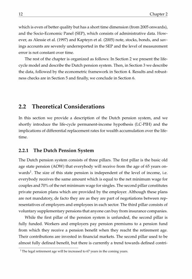
2.2.1 The Dutch Pension System
The Dutch pension system consists of three pillars. The first pillar is the basic old
age state pension (AOW) that everybody will receive from the age of 65 years on-
wards1. The size of this state pension is independent of the level of income, i.e.
everybody receives the same amount which is equal to the net minimum wage for
couples and 70% of the net minimum wage for singles. The second pillar constitutes
private pension plans which are provided by the employer. Although these plans
are not mandatory, de facto they are as they are part of negotiations between rep-
resentatives of employers and employees in each sector. The third pillar consists of
voluntary supplementary pensions that anyone can buy from insurance companies.
While the first pillar of the pension system is unfunded, the second pillar is
fully funded. Workers and employers pay pension premiums to a pension fund
from which they receive a pension benefit when they reacht the retirement age.
Their contributions are invested in financial markets. The second pillar used to be
almost fully defined benefit, but there is currently a trend towards defined contri-
1 The legal retirement age will be increased to 67 years in the coming years.

Education level and age-wealth profiles 13
bution. It is important to stress that the wealth data in this study does not include
occupational pension wealth that is accumulated in the second pillar. The latter rep-
resents a large fraction of Dutch household wealth (Van Ooijen et al., 2015), but, as
explained above, our interest lies in saving behavior conditional on a given pension
arrangement.
The retirement replacement rate is defined as the ratio between net pension in-
come from the first two pillars and net labor income just before retirement. Due to
the existence of the first pillar with its flat benefit level, the Dutch pension system is
redistributive in nature, which implies that the retirement replacement rate will be
decreasing in the level of income. The benchmark gross replacement rate is about
70% for a median career worker, although net replacement rates are a bit higher as
retirees do not pay social security taxes and pension premiums (Van Duijn et al.,
2013).
2.2.2 Life Cycle Model
The LC-PIH states that individuals (or households) will consume a constant frac-
tion of their lifetime income. Because, in general, labor income shows an upward
sloping profile until retirement and suddenly drops afterwards, individuals will
accumulate wealth while working in order to finance consumption during retire-
ment. The theory was originally developed by Modigliani and Brumberg (1954)
and Friedman (1957).
In its most simple form, it implies that wealth W at time t is equal to accumu-
lated savings (see e.g. Kapteyn et al. (2005)), i.e.:
Wt = W0 +t
∑τ=1
(yτ − YPτ ),
where we assume for simplicity that the interest rate and the rate of time preference
are equal to zero. Furthermore, W0 is initial wealth, yτ is non-capital income at time
τ and YPτ is permanent income2 at time τ. Thus, the theory says that individuals
will save the difference between current income and permanent income. If labor
income is more or less hump-shaped over the lifetime, saving should be positive
before retirement and negative after retirement.
Because a perfectly hump-shaped age-wealth profile was hardly ever found
in the first generation of empirical studies about the LC-PIH (King and Dicks-
2 Permanent income is defined as the annuity value of present and future income (Kapteyn et al., 2005).

14 Chapter 2
Mireaux, 1982), the original theory has been adapted in several ways. For example,
if households have a bequest motive wealth may not decline at all after retire-
ment because households behave as if they have an infinite horizon (Barro, 1974,
Hurd, 1989). Also, if agents have a precautionary saving motive the standard life-
cycle model with intertemporally additive quadratic utility functions, perfect cap-
ital markets and perfect certainty (or agents maximizing expected utility) may offer
very unreliable predictions of saving behavior (Browning and Lusardi, 1996). Fi-
nally, the behavioral life-cycle model (Shefrin and Thaler, 1988) takes into account
the problem of self-control, which causes individuals to depart from rational beha-
vior.
There is a very large empirical literature that examines age-wealth profiles (or
saving rates) with micro-data (see Browning and Lusardi (1996) for a survey). How-
ever, there are only a few studies that explicitly investigate differences in wealth
accumulation between educational groups. Solmon (1975) already finds that edu-
cation has a positive effect on saving rates. He uses a cross-section of households
and explicitly looks for a causal effect from education to saving rates. However, in
this study we are investigating differences in saving behavior between groups with
different educational attainment, and not looking for a direct effect from education
to saving.
For the Netherlands, Alessie et al. (1997) find a hump-shaped age-wealth pro-
file for highly educated households and a relatively flat profile for low-educated
households, while Hubbard et al. (1995) conclude the same for the U.S. Avery and
Kennickell (1991), Bernheim and Scholz (1993) and Attanasio (1998) all find higher
saving rates for highly educated households than for low-educated households in
the U.S. According to Browning and Lusardi (1996), these findings are difficult to
reconcile with the standard LC-PIH. However, if the institutional setting in the
U.S. is comparable to the Netherlands (the expected retirement replacement rate
is decreasing in educational attainment) this is doubtful. Our hypothesis is that
these differences can be explained by differences in expected retirement replace-
ment rates between educational groups.
The effect of differences in replacement rates on wealth accumulation can be ex-
amined quite easily in a life-cycle permanent-income framework. The well-known
consumption Euler equation is given by:
U′(Ct) = Et[U′(Ct+1)1 + r1 + ρ
],

Education level and age-wealth profiles 15
where U(.) is an intratemporal utility function that is assumed to be strictly concave
and maximized by the agent, Ct is consumption in period t, r is a constant real
interest rate and ρ is the rate of time preference. If we assume that agents have
access to a risk-free asset with return r, that r = ρ, and that the utility function is
quadratic, the following holds (Hall, 1978):
Ct = Et[Ct+1]. (2.1)
So, expected consumption in period t + 1 equals consumption in period t. In other
words, consumers will smooth consumption over their lifetime.
To illustrate the effect of the retirement replacement rate consider a two-period
consumption model. In the first period, the agent works and in the second period
he or she is retired. Let Y1 be (labor) income in period 1 and Y2 be (pension) income
in period 2. Furthermore, let θ be the retirement replacement rate, equal to Y2Y1
. There
is no lifetime uncertainty and r = ρ = 0. According to equation (2.1), consumption
will be equalized across periods. Thus, C1 = C2 = (1+θ)Y12 . Saving S in period 1 and
2 is given by, respectively S1 = Y1 − C1 = 1−θ2 Y1 and S2 = Y2 − C2 = θ−1
2 Y1.
This shows that in the most simple model the saving rate S/Y only depends on
the retirement replacement rate θ. In addition, by assuming homothetic preferences
S/Y does not contain productivity-related cohort effects anymore. Furthermore, a
lower retirement replacement rate (lower θ) increases saving before retirement (S1)
and decreases saving (increases dissaving) after retirement (S2). Of course, in this
simple set-up saving and dissaving are exactly equal to each other. However, we
abstract from other saving motives such as precautionary saving. If such a motive
would be present, the total level of saving would be higher before retirement. On
the other hand, if households keep saving for precautionary reasons after retire-
ment we might not observe any dissaving at all (see De Nardi et al. (2009, 2010)).
Van Santen et al. (2012) report that the average expected retirement replacement
rate is decreasing in the level of education in a sample of about 600 Dutch individu-
als over the period 2007-2009. Note that their data is about expected replacement
rates, which do not necessarily equal realized replacement rates, as Bottazzi et al.
(2006) and Van Duijn et al. (2013) show. However, individuals base their saving de-
cisions, among other things, on expected replacement rates as they do not know yet
what their realized replacement rate will be in the future. Therefore, expected re-
placement rates are the right measure to use. For individuals with only elementary
education they find an expected replacement rate of 88%, for secondary-educated

16 Chapter 2
81%, for college-educated 76% and for university-educated 75%. Correcting for the
level of income, this implies that highly educated households have a higher saving
rate than low-educated households in order to smooth consumption over the life-
time.
2.3 The Data
We base our empirical analyses on the DNB Household Survey (DHS). Since 1993,
about 2500 Dutch households of the CentERpanel3 are asked, on a yearly basis, to
fill in a questionnaire with questions about their financial position, labor market
position, household characteristics, and health status. The questions relate to the
past year. For example, in the questionnaire of 1993 information should be provided
about the level of several asset and debt categories on the 31st of December 1992.
We use the waves from 1995 onwards, as the data of the first two waves is too
incomplete and unreliable to use in a panel data analysis. Up to 1999 the house-
holds are divided into two panels, one with a representative sample of the Dutch
population and the other with a random sample of households in the highest in-
come decile (the high-income panel). The representative panel consists of about
2000 households and the high-income panel of about 500 households. From 2000
onwards the dataset only contains the representative panel. We will perform our
benchmark analyses with the representative panel, but will estimate all models
with the households from the high-income panel included as well as a robustness
check. However, all summary statistics that we show concern only the representat-
ive sample. Note that we do not use sample weights, so our summary statistics are
not corrected for possible over- or underrepresentation of certain groups.
We take the household, and not the individual, as our unit of analysis. The main
rationale for this choice is that the data does not allow a clear separation of wealth
between different household members.4 Besides that, in most households financial
decisions will be taken at the household level, not at the individual level. One of
the drawbacks of this method is that households, unlike individuals, do not have
a unique birth year. We take the birth year of the oldest household member as the
birth year of the household and the highest education level within the household
3 A group of about 2500 households that form a good representation of the Dutch population.4 Although in principle each household member fills in a questionnaire, it turns out to be impossible to
determine wealth levels on an individual basis.

Education level and age-wealth profiles 17
as the education level of the household. The appendix explains how the different
education levels are defined. Note that for households where the level of education
is time-invariant we take the mode. For couple households, we simply add wealth
and income of both household members to arrive at wealth and income levels of
the household.
We drop all children, grandparents and ’other members of the household’ to
make sure that every household consists of either one or two adult persons. Ignor-
ing the wealth of possible children in the household is justified because children
normally take their wealth with them when they leave the parental home5. We
also drop all individuals who are self-employed as their financial position is too
complicated to be used for a test of the life-cycle model. Furthermore, we drop all
individuals for whom the birth year is unknown. Finally, because there exists a
positive correlation between wealth levels and life expectancy (Jappelli, 1999, At-
tanasio and Hoynes, 2000), we confine ourselves to households with a head who
is younger than 80 years old to prevent a bias towards wealthy households in the
advanced age categories.
One of the well-known problems with survey data concerns measurement er-
ror. Although it is impossible to filter out all unreliable observations, we do try to
identify and drop the most obvious ones. To begin with, we delete all households
that report housing wealth above 10 million euros, which are only four households.
Furthermore, we drop all observations where households report mortgage debt,
but their house has a value of zero. This would mean that they do not own the
house anymore, so a possible mortgage debt should not be counted as negative
housing wealth but rather as negative financial wealth. Besides that, we suspect
that most of these cases concern measurement error as well. All in all, this amounts
to 102 observations.
Following Kapteyn et al. (2005) we use financial net wealth and total net wealth.
The difference between the two wealth measures is that the former excludes hous-
ing wealth. The appendix provides exact details about the construction of both
wealth measures. Some of the asset catgories that we include merit a bit of clari-
fication. Browning and Lusardi (1996) discuss several issues related to the proper
definitions of saving and wealth. One of these concerns the treatment of consumer
durables. The life-cycle model assumes that consumers derive utility from the con-
sumption of service flows rather than consumption expenditures, which implies
5 Although it is difficult to determine wealth levels on an individual basis for adult members of thehousehold, it is possible for children. Note that this is an advantage of the DHS which, unlike mostother datasets, presents wealth on the individual level instead of the household level.

18 Chapter 2
that the investment in durable consumption goods should be considered as sav-
ing to be consistent with the theory (Hendershott and Peek, 1989). Therefore, we
include the value of consumer durables, such as cars, boats and caravans, in our
definition of wealth.
Households that report missing values for all asset and debt categories are de-
leted from the sample. However, if they do report an amount (which may be even
zero) in at least one category, all the other missing values of that particular house-
hold are assumed to be equal to zero. The reason for this assumption is that it
provides us with additional observations, which would be lost if we simply de-
lete all observations with at least one missing value in an asset or debt category. We
believe it is reasonable to assume that for these households missing values consti-
tute a value of zero, because they have provided at least one value for an asset or
debt category. We deflate wealth levels by the Consumer Price Index that Statistics
Netherlands (CBS) provides to ensure that all wealth levels are in real terms (1994
euros).
Table 2.1 shows summary statistics for net disposable income, financial net wealth,
total net wealth, permanent income, financial net wealth divided by permanent in-
come, and total net wealth divided by permanent income. All income measures in
this study are after-tax as the DHS provides a net income variable. In the next sec-
tion we will explain in detail how we calculate permanent income. Note that for
financial net wealth as well as total net wealth the mean is much higher than the
median, which is common in wealth data. Furthermore, the distance between the
3rd quartile and the median is larger than the distance between the 1st quartile and
the median. This implies that the wealth distribution is rightly skewed. This is still
the case after scaling by permanent income.
In total, we have 21,246 observations consisting of 5,918 different households,
which means that each household is on average covered three to four times in the
data set. Income data is missing for about 400 observations, but as we explain in
the next section we predict these income levels so that we can use them to calculate
permanent income.
Tables 2.2 and 2.3 present median financial net wealth and median total net
wealth per age class for the full sample, and for each education category separ-
ately. The medians are taken over all cohorts and time periods, and are as such
not a definitive indicator of a certain age-wealth profile for individual households.
As expected, both financial net wealth and total net wealth are increasing in edu-
cation level, although the values in the lowest age categories for households with

Education level and age-wealth profiles 19
Table 2.1. Summary statistics
Income FNW TNW YP FNW/YP TNW/YP
Observations 20,868 21,246 21,246 21,246 21,246 21,246Households 5,741 5,918 5,918 5,918 5,918 5,918Mean 22,326 31,072 103,561 17,928 1.847 6.185Standard Deviation 29,649 69,501 152,042 7,620 4.184 9.1121st Quartile 14,118 3,480 7,471 12,930 0.211 0.475Median 19,546 14,058 53,232 16,664 0.816 3.0653rd Quartile 26,641 35,275 151,367 21,498 2.143 8.905
Notes: All monetary amounts are in 1994 euros. FNW = Financial Net Wealth, TNW = Total Net Wealth, YP =Permanent Income. All income measures are after-tax.
a university degree are somewhat lower than expected. This could be due to the
relatively steep income profile highly educated people experience, which implies
that, in the absence of liquidity constraints, they will borrow in the beginning of
their adult lives (Lopes, 2008).
The main difference between financial net wealth and total net wealth, apart
from the fact that the latter is consistently higher, is that total net wealth hardly
declines after retirement (except for households with only elementary education)
while financial net wealth does for the two highest education categories (’college’
and ’university’). This could imply that, while highly educated households do seem
to run down financial assets to some extent after retirement, they do not sell their
house in order to satisfy their consumption needs. However, it is important to stress
that age and cohort effects are not disentangled in tables 2.2 and 2.3. The age-wealth
patterns that these tables seem to reveal should therefore be interpreted with cau-
tion.
Tables 2.4 and 2.5 present the same information as tables 2.2 and 2.3, but with
wealth levels scaled by permanent income. The patterns are comparable to tables
2.2 and 2.3. These raw statistics already suggest that the higher households are edu-
cated the more wealth they accumulate, even after scaling for permanent income.

20 Chapter 2
Table 2.2. Median financial net wealth per age category and level of education
Age Full Sample Elementary Secondary College University20-24 1,815 0 653 3,577 2,41525-29 4,400 3,112 2,607 7,198 5,32430-34 7,903 4,402 6,390 10,373 9,74535-39 10,421 4,968 9,269 13,356 14,40040-44 12,002 5,250 11,036 17,223 18,89545-49 12,840 7,274 10,458 18,326 24,72850-54 16,289 10,516 15,130 20,719 30,63155-59 20,631 14,883 16,855 28,261 34,15560-64 23,696 17,827 19,422 30,519 60,57965-69 24,104 13,426 25,722 28,384 57,57270-74 24,815 17,734 25,992 25,459 53,66675-79 24,183 16,733 24,439 28,788 33,086
Note: All monetary amounts are in 1994 euros. The educational groups are determined as follows: Survey parti-cipants who choose ’WO’ are university-educated, participants who choose ’HBO’ are college-educated and par-ticipants who choose either ’HAVO/VWO’ or ’MBO’ are secondary educated. All other participants are definedto be in the elementary-educated group. The level of education is at the household level, taking the highest level ifthere are two household members.
Table 2.3. Median total net wealth per age category and level of education
Age Full Sample Elementary Secondary College University20-24 2,256 123 1,826 3,766 3,10925-29 6,131 4,061 4,329 11,195 5,62030-34 15,941 16,477 13,157 20,389 12,54535-39 32,769 14,161 28,234 48,925 34,98340-44 50,102 17,587 42,405 65,063 66,31345-49 61,222 31,646 54,322 86,240 84,15150-54 73,048 32,332 62,268 97,849 115,83155-59 97,537 63,958 76,360 124,389 185,77860-64 114,045 57,597 99,859 162,387 232,35265-69 113,046 31,355 116,644 136,629 227,33370-74 124,634 40,554 129,552 130,034 259,62875-79 100,176 30,110 97,682 159,069 219,990
Note: All monetary amounts are in 1994 euros. The educational groups are determined as follows: Survey parti-cipants who choose ’WO’ are university-educated, participants who choose ’HBO’ are college-educated and par-ticipants who choose either ’HAVO/VWO’ or ’MBO’ are secondary educated. All other participants are definedto be in the elementary-educated group. The level of education is at the household level, taking the highest level ifthere are two household members.

Education level and age-wealth profiles 21
Table 2.4. Median financial net wealth divided by permanent income per age category andlevel of education
Age Full Sample Elementary Secondary College University20-24 0.055 0.000 0.026 0.133 0.07125-29 0.180 0.150 0.133 0.271 0.14530-34 0.349 0.215 0.336 0.416 0.31135-39 0.522 0.313 0.521 0.601 0.63140-44 0.670 0.354 0.617 0.844 0.90845-49 0.777 0.450 0.674 0.988 1.35150-54 1.041 0.748 1.042 1.131 1.81455-59 1.378 1.127 1.227 1.616 2.21560-64 1.720 1.458 1.479 1.877 3.89365-69 1.774 1.262 1.786 1.899 3.82270-74 1.966 1.700 1.903 1.890 3.49175-79 1.859 1.643 1.990 2.177 2.022
Note: All monetary amounts are in 1994 euros. The educational groups are determined as follows: Survey parti-cipants who choose ’WO’ are university-educated, participants who choose ’HBO’ are college-educated and par-ticipants who choose either ’HAVO/VWO’ or ’MBO’ are secondary educated. All other participants are definedto be in the elementary-educated group. The level of education is at the household level, taking the highest level ifthere are two household members.
Table 2.5. Median total net wealth divided by permanent income per age category and levelof education
Age Full Sample Elementary Secondary College University20-24 0.090 0.004 0.048 0.142 0.09025-29 0.260 0.232 0.220 0.406 0.15530-34 0.701 0.793 0.703 0.806 0.47335-39 1.524 0.770 1.502 2.194 1.20840-44 2.791 1.174 2.792 3.177 3.42045-49 3.628 2.056 3.373 4.352 5.15550-54 4.428 2.183 4.002 5.443 7.17455-59 6.567 4.704 5.705 7.300 10.77060-64 7.918 5.100 6.986 9.658 13.18165-69 8.051 2.654 8.414 9.568 13.91170-74 9.389 3.579 10.289 9.226 15.23175-79 8.365 2.911 7.746 11.295 12.832
Note: All monetary amounts are in 1994 euros. The educational groups are determined as follows: Survey parti-cipants who choose ’WO’ are university-educated, participants who choose ’HBO’ are college-educated and par-ticipants who choose either ’HAVO/VWO’ or ’MBO’ are secondary educated. All other participants are definedto be in the elementary-educated group. The level of education is at the household level, taking the highest level ifthere are two household members.

22 Chapter 2
2.4 Econometric Framework
In the first part of this section we explain our empirical strategy and in the second
part we show how we calculate permanent income.
2.4.1 Empirical Strategy
Panel data on wealth usually contains age, time and cohort effects. Age effects are
what we are ultimately interested in in this study. Time effects especially capture the
business cycle and the corresponding movement on financial markets, which affect
wealth levels. Cohort effects arise if different cohorts have different levels of per-
manent income due to differences in productivity levels across generations (Shor-
rocks, 1975). They can also be caused by different attitudes towards saving between
different generations. People who grew up during the Great Depression might be
thriftier than generations who grew up in times of an economic boom, such as the
post-war period. It is important to account for all these three effects when estim-
ating age-wealth profiles. Failing to take cohort effects into account might give the
impression of a hump-shaped age-wealth profile if older cohorts have lower aver-
age wealth holdings than younger cohorts.
It is impossible to estimate age, time and cohort effects directly in a panel be-
cause calendar year is equal to age plus year of birth (cohort). In such a model the
parameters are not identified. One could assume that there are either no cohort or
no time effects present in the data, but these assumptions may not be justified given
past evidence. An alternative is to use the approach of Deaton and Paxson (1994).
Their solution to the identification problem is to assume that the coefficients on the
year dummies sum to zero and are orthogonal to a time trend. This implies that the
time effects are only a reflection of business cycle effects that average out over the
full sample period. However, we believe that the assumption that the year dum-
mies sum to zero is not plausible in the case of wealth data, as (financial) wealth is
a stock variable which depends on past income shocks.
Jappelli (1999) uses the fact that consumption is proportional to lifetime re-
sources as long as preferences are homothetic. This implies that subtracting (the
log of) consumption from both sides of a wealth regression drops the cohort effect
from the right-hand side of the equation. He then regresses the log of the wealth-
consumption ratio on an age polynomial, a set of unrestricted time dummies, and
some household characteristics. Unfortunately, the DHS does not contain data on
consumption, so the approach of Jappelli (1999) is not feasible for us.

Education level and age-wealth profiles 23
We therefore choose a different strategy, namely dividing wealth by permanent
income. In that case, all productivity-related cohort effects are incorporated in the
dependent variable as long as quadratic utility is assumed.6 Possible differences in
preferences between different cohorts are not captured in this way. However, for
example Kapteyn et al. (2005) show that permanent income and changes in Social
Security can explain all cohort differences in wealth in their sample of Dutch house-
holds. We therefore believe that our approach captures most of the cohort effects.
To estimate age and time effects we use a linear spline function in age and a normal
set of time dummies. The spline function in age has four knots with the fourth one
exactly defined at the legal retirement age of 65.
We also include a set of selectivity dummies and a set of learning dummies7. The
selectivity dummies are meant to capture the idea that households that drop out of
the sample might be different from households that participate at least one more
year. The learning dummies pick up the effect that households might get better or
worse in filling in the questions of the survey as they participate (Kapteyn et al.
(2005)).
Attanasio and Browning (1995), among others, argue that changes in consump-
tion needs due to changing household characteristics are important for the explan-
ation of wealth profiles. Therefore, we include a dummy for couple households and
the number of children in the house as control variables. Finally, we add a dummy
for living in an urban area, and regional dummies for each province of the Nether-
lands. The basic model that we estimate is then as follows:
Wht
YPh
=5
∑i=1
ζisi(ageht) + γt + X′ht β + ϵht, (2.2)
where Wht is wealth of household h in year t, YPh is permanent income of household
h, si is a linear spline function in age, ageht is the age of the head of household h
in year t, γt is a time fixed effect for year t, Xht is a matrix of control variables
discussed above and ϵ is the error term with conditional median zero. Finally, the
ζi, and the elements of the parameter vector β are coefficients to be estimated.
6 In the next section we explain how permanent income is constructed.7 The selectivity dummy is one in year t if the household participates in year t and at least one more
time after year t, and zero otherwise. The first learning dummy is one if the household participates inthat year for the first time, the second learning dummy is one if the household participates in that yearfor the second time, etc.

24 Chapter 2
Note that Med(ϵht|ageht, Xht) = 0 as we assume that WhtYP
hdoes not contain
any cohort effects anymore. We estimate equation (2.2) for all four education cat-
egories. However, we also want to examine the differences in age-wealth profiles
between low- and highly educated households in one regression framework. There-
fore, we define a dummy variable edu that equals one for highly educated house-
holds (college- and university-educated) and zero for low-educated households
(elementary- and secondary-educated). Then, we construct the interaction variables
agei ∗ edu for i = 1,2,...,5.
Adding the interaction effects and the education dummy to equation (2.2) gives
the following regression model:
Wht
YPh
=5
∑i=1
ζisi(ageht) +5
∑i=1
ϕisi(ageht ∗ eduh) + θ eduh + γt
+ X′ht β + ϵht, (2.3)
Note that we assume the level of education to be time-invariant by taking the mode
for each household8. Because the wealth distribution is rightly skewed and we
expect influential outliers to be present, we estimate equations (2.2) and (2.3) by
median regression instead of OLS. To account for heteroskedasticity and within-
household dependence over time we compute cluster-bootstrapped standard er-
rors.
2.4.2 Permanent Income
By definition, permanent income is not observed for individuals who are still alive.
We therefore have to estimate it from the available information. Our strategy to
estimate permanent income consists of three steps: First, we regress current income
on a linear spline function in age, a set of Deaton-Paxson time dummies (see Deaton
and Paxson (1994)), some household characteristics, and a household fixed effect.
Then, based on the regression results we forecast future income levels, and backcast
past income levels. In case we have data on past or future household income we
replace the predicted value by the observed value. Finally, we calculate permanent
income from current income and the predicted levels of past and future income.
8 Respondents could make mistakes in filling in the questionnaire, or alternatively, the level of educa-tion might change over time if the respondent pursues an education during the survey period.

Education level and age-wealth profiles 25
While we choose not to use Deaton-Paxson time dummies for the wealth regres-
sions, we do think they are suitable to model income. As explained above, Deaton
and Paxson (1994) assume that the coefficients on the year dummies sum to zero
and are orthogonal to a time trend, which implies that they are only a reflection of
business cycle effects. While it is hard to argue that this is the case for wealth, it
seems a reasonable assumption for income. Furthermore, it allows us to estimate a
cohort effect as well. We will describe below how we model the cohort effect.
Our model for permanent income largely follows Kapteyn et al. (2005). The
main differences are: First, we backcast and forecast non-capital income, while
Kapteyn et al. (2005) only forecast income. Second, Kapteyn et al. (2005) do not
use Deaton-Paxson time dummies in their income regressions, while we do. If real
GDP per capita around the time the household entered the labor market is used
as a control variable, Deaton-Paxson time dummies are not necessary anymore to
identify the coefficients of the model. However, we prefer to model the time effects
in this way as the coefficients on the dummies sum to zero, which allows us to ig-
nore time effects in backcasting income. This would not be allowed when we had
estimated regular time effects.
As the income data comes from questionnaires it is subject to measurement er-
ror. In general we have no reason to assume that this measurement error is non-
random. However, there seems to be one exception. Some older households, espe-
cially in the lowest education category, report income levels that are too low to be
correct. In the Netherlands, every individual above the age of 65 receives a Social
Security Benefit (AOW in Dutch). We observe some households with incomes that
are (much) lower than the amount of AOW they should receive9. Therefore, we set
an income floor for households with a head who is at least 65 that equals the level
of the AOW benefit.
To estimate current income we largely follow the model of Kapteyn et al. (2005):
log(yht) =5
∑i=1
βisi(ageht) + γ∗t + X
′htρ + uh + ϵht, (2.4)
where yht is net income of household h in year t, si is a linear spline function in age,
ageht is the age of the head of household h in year t, γ∗t is a Deaton-Paxson time fixed
effect, and X consists of a set of learning dummies, a set of selectivity dummies, the
9 The only exception yields people who lived abroad between the age of 15 and 65. Their income couldbe lower than the standard level of the AOW benefit. However, we believe that, especially among thelow-educated, this does not play an important role here.

26 Chapter 2
number of children in the house and a dummy variable for couple households. The
reason for including this dummy is that the level of income depends on whether a
household consists of one or two adults, especially when receiving Social Security
benefits after retirement. We model the individual effect uh (the Mundlak term) as
follows (see Mundlak (1978)):
uh = W ′h θ + δ log(rgdpch) + vh, (2.5)
where Wh consists of the time averages of all time-varying explanatory variables
in equation (2.4) for household h, rgdpch is a cohort-specific variable, which is the
average level of real GDP per capita around the time household h entered the labor
market. This should capture possible cohort effects. We calculate average real GDP
per capita for the years when the household head was between 16 and 25 years
old. Finally, vh is an individual effect that we assume to be random and uncorrel-
ated with the explanatory variables in (2.4). Modeling the individual effects in this
way, we let them depend on household specific means of all time-varying right-
hand side variables and a cohort effect. We insert equation (2.5) into equation (2.4)
and then estimate the latter by the random effects estimator. To allow for intra-
household correlation we calculate clustered standard errors. As especially educa-
tion level and marital status are powerful indicators of lifetime earnings (Hurd et
al., 2012) we estimate separate models for each different education category.
The learning dummies turn out to be jointly insignificant. This means that learn-
ing does not seem to play a role when respondents fill in the questionnaire. The se-
lectivity dummies are also jointly insignificant, which suggests that there is no evid-
ence of endogenous attrition in our sample (see Verbeek and Nijman (1992)). We
therefore drop the learning dummies and selectivity dummies. Table 2.6 presents
the estimation results.
The age spline variables and the Deaton-Paxson time dummies are jointly sig-
nificant for all educational groups. Furthermore, the log of rgdpc around the time
the household entered the labor market is positively significant for all education
groups. This suggests that, controlling for age and time effects, households who
entered the labor market in periods with low productivity, for example during a re-
cession, experience a lower level of income during the rest of their lives, compared
to households who started their working career in a high productivity period.
We also test whether the Mundlak terms that make up the individual effects are
jointly significant, which they are for all groups. If they would have been insigni-

Education level and age-wealth profiles 27
ficant we could just as well have estimated a standard random effects model, but
their significance justifies modeling the individual effects as we do. As expected, the
partner dummy is positively significant, the level of income of couple households
is on average around 28% higher than the income of singles, while the number of
children in the house does not seem to be an important predictor of income. To
get a clearer idea of the age-income profiles that these results imply, we turn to a
graphical presentation.
Figure 2.1 shows education-specific age-income profiles. The dashed lines rep-
resent the 95% confidence bounds. As expected, a higher level of education is as-
sociated with a higher level of income. Especially university-educated workers ex-
perience a relatively steep income profile during the first few years of their work-
ing career. This is one of the causes of the difference in replacement rates between
them and low-educated households. After retirement, income drops gradually for
university-educated households, and stays more or less constant for the other three
educational groups. This is in line with our expectation that replacement rates are
lower for highly-educated households in the Netherlands.
68
1012
14lo
g(in
com
e)
20 40 60 80age
elementary
68
1012
14lo
g(in
com
e)
20 40 60 80age
secondary
68
1012
14lo
g(in
com
e)
20 40 60 80age
college
68
1012
14lo
g(in
com
e)
20 40 60 80age
university
Figure 2.1. Age-income profiles (solid lines) for four different education categories.The dashed lines represent 95% confidence bounds.
Subsequently, we use the coefficient estimates as presented in table 2.6, to pre-

28 Chapter 2
dict past and future incomes. Of course, the evolution of income is mainly driven
by age. However, following Kapteyn et al. (2005), we also want to take into account
that household characteristics might change if people age. We therefore update the
number of children in the house and the presence of a partner as well. In order to
be able to do this we estimate the following fixed effects regression model and use
the coefficient estimates to predict how the number of children in the house and the
probability of a partner change when the household ages:
zht = µh +79
∑a=21
ϕaageh + uht,
where zht is the number of children in the house or the presence of a partner of
household h in year t, µh is a household fixed effect, ageh is an age dummy and uht
is a random error term with mean zero. We assume that education level is time-
invariant, when we backcast and forecast income. Furthermore, we set all time
dummies to zero, as we have modeled them as pure business cycle effects. Finally,
we set the learning dummies and selectivity dummies equal to zero.
We have income data (either directly from the questionnaire or imputed) for
approximately 98% of the sample. However, we do predict past, current, and fu-
ture income of households for which income data is missing, by assuming that the
individual effect equals zero for them. Then, permanent income in year t equals:
YPh =
Wh0 + ∑Tτ=0(1 + r)−τ yhτ
∑Tτ=0(1 + r)−τ
,
where yhτ is the predicted value of yhτ . Note that yhτ includes vh. The equation
above states that permanent income is a weighted average of the present values of
all past, current, and future incomes, where the discount factors form the weights.
In case all incomes would be exactly equal to each other, these would also be equal
to permanent income. One of the simplifications that we make is that we set wealth
at the age of 20, Wh0, equal to zero. We assume that the interest rate r is fixed and
equal to 3%. Furthermore, we only calculate future income until the age of 80 and
assume that it is zero afterwards (or equivalently, that people die at the age of 80).
This means that T equals 59 in the equation above. To keep things as simple as
possible, we ignore survival probabilities because the effect will be negligible.

Education level and age-wealth profiles 29
Table 2.6. Income Regression Estimates
Dependent variable log(Income)Education level elem sec coll uniage 20-32 0.026 0.037 0.040 0.107
(0.033) (0.010)*** (0.010)*** (0.015)***age 32-43 0.043 0.026 0.032 0.059
(0.014)*** (0.005)*** (0.006)*** (0.011)***age 43-54 0.009 0.017 0.019 0.024
(0.006) (0.004)*** (0.004)*** (0.006)***age 54-65 0.003 -0.002 0.005 0.004
(0.006) (0.005) (0.005) (0.011)age 65-79 0.007 0.009 0.007 -0.004
(0.005) (0.004)** (0.005) (0.012)log(rgdpc) 0.638 0.535 0.478 0.569
(0.087)*** (0.088)*** (0.070)*** (0.118) ***partner dummy 0.232 0.281 0.272 0.245
(0.080)*** (0.056)*** (0.052)*** (0.134)*number of children 0.006 0.003 0.032 -0.022
(0.026) (0.018) (0.019)* (0.031)p-value χ2-test joint sign. 0.004 0.000 0.000 0.000age spline variablesp-value χ2-test joint sign. 0.000 0.000 0.000 0.002Deaton-Paxson time dummiesp-value χ2-test joint sign. 0.004 0.001 0.032 0.014Mundlak effectsNumber of observations 4,736 7,117 6,212 2,803Number of households 1,278 1,949 1,699 815R2 0.20 0.20 0.21 0.25
Notes: Estimated by random effects. Numbers in parentheses are clustered standard errors. *,**,*** denote sig-nificance at the 10%, 5% and 1% respectively. log (rgdpc) is het natural logarithm of the average level of realGDP per capita around the time the household entered the labor market. Deaton-Paxson time dummies are in-cluded in the specification but the individual estimates are not reported. The educational groups are determined asfollows: Survey participants who choose ’WO’ are university-educated (uni), participants who choose ’HBO’ arecollege-educated (coll) and participants who choose either ’HAVO/VWO’ or ’MBO’ are secondary educated (sec).All other participants are defined to be in the elementary-educated group (elem). The level of education is at thehousehold level, taking the highest level if there are two household members.

30 Chapter 2
2.5 Results
In this section we present the regression results. First, we show the results from es-
timating equation (2.2) for different education categories. Second, we present and
discuss the results from estimating equation (2.3). Finally, we show results from
estimating all specifications with the households from the high-income panel in-
cluded.
Table 2.7 presents the results of estimating equation (2.2) for all four different
education categories. The dependent variables are financial net wealth divided by
permanent income (columns 1-4), and total net wealth divided by permanent in-
come (columns 5-8). All regressions include a full set of time dummies, but we
drop the selectivity dummies and learning dummies as they both are jointly insig-
nificant.
The age spline variables are jointly significant in all eight regressions. The time
dummies and regional dummies are jointly significant in some of them. Further-
more, the partner dummy is positively significant for most educational groups
but is negative for university-educated households. The number of children in the
house has a negative effect on wealth accumulation, but only when housing wealth
is excluded. Finally, households in urban areas seem to save relatively more than
households in rural areas.
The coefficients on the age spline variables for financial wealth show a pat-
tern that is more or less consistent with our expectations. Households accumulate
wealth during the working span of their lives but only university-educated house-
holds decumulate wealth after retirement. Note that our finding that the coefficient
on age 65-79 is positive for elementary-, secondary-, and college-educated house-
holds does not necessarily imply that they do not decumulate retirement-related
wealth after the age of 65. If they have a strong precautionary saving motive, this
effect might undo the negative wealth effect of decumulation for retirement pur-
poses. In that case we would still observe a positive coefficient estimate. However,
it is clear that university-educated households decumulate wealth much faster after
retirement.
It is essential to realize that we find these patterns while correcting wealth
for the level of permanent income. Our findings are thus not merely a reflection
of the fact that highly educated households have higher levels of income than
low-educated households, but indicate that even if income would be equal across
groups highly educated households accumulate more wealth before retirement and
decumulate wealth after retirement. This is exactly what the LC-PIH predicts, con-

Education level and age-wealth profiles 31
sidering the fact that the retirement replacement rate differs between groups with
different educational attainment.
−1
01
23
45
fin. w
ealth
/per
m. i
ncom
e
50 60 70 80age
first quartile
−1
01
23
45
fin. w
ealth
/per
m. i
ncom
e
50 60 70 80age
second quartile−
10
12
34
5fin
. wea
lth/p
erm
. inc
ome
50 60 70 80age
third quartile
−1
01
23
45
fin. w
ealth
/per
m. i
ncom
e
50 60 70 80age
fourth quartile
Figure 2.2. Age-financial wealth profiles (solid lines) for four different educationcategories. The dashed lines represent 95% confidence bounds.
Figure 2.2 shows the age-financial wealth profiles that the regression results im-
ply. All other variables are evaluated at their means. The dashed lines represent the
95% confidence bounds. It is clear that the profile of university-educated house-
holds differs quite significantly from the others. These highly educated households
save a lot more before retirement, and dissave after retirement. In contrast, the other
educational groups do not save that much before retirement, and do not dissave
after retirement.
Figure 2.3 presents the age-wealth profiles for total net wealth. They are compar-
able to the profiles for financial net wealth in the pre-retirement phase. However,
after retirement university-educated households keep accumulating wealth. This
suggests that university-educated households in general do not sell their house in
order to finance consumption after retirement, because we find a smaller coeffi-
cient for age 65-79 when excluding housing wealth (see table 2.7). This finding is
consistent with the conclusions of, for example, Venti and Wise (1990). In addition,
Alessie et al. (1995) show that Dutch elderly finance consumption mainly through

32 Chapter 2
−1
37
1115
tota
l wea
lth/p
erm
. inc
ome
50 60 70 80age
first quartile
−1
37
1115
tota
l wea
lth/p
erm
. inc
ome
50 60 70 80age
second quartile
−1
37
1115
tota
l wea
lth/p
erm
. inc
ome
50 60 70 80age
third quartile
−1
37
1115
tota
l wea
lth/p
erm
. inc
ome
50 60 70 80age
fourth quartile
Figure 2.3. Age-total wealth profiles (solid lines) for four different education cat-egories. The dashed lines represent 95% confidence bounds.
Social Security (AOW) and occupational pensions, and not by selling their house
(or taking up a second mortgage on their house). A possible explanation might be
that highly-educated households, because they are healthier on average, are able to
stay longer in their own house, compared to low-educated households who might
be forced by their health condition to sell their house (if they own one) and spend
the last few years of their lives in a nursing home.
Jappelli and Modigliani (2006) discuss a possible bias in measures of wealth
levels at advanced ages. As people respond to the survey in the next period, only
the survivors are physically able to do so. However, there is a negative correlation
between mortality and wealth (see, among others, Hurd et al. (2001)), which means
that the survivors are on average richer than the deceased. This would mean that
the sample is biased towards rich individuals, especially for the advanced age cat-
egories. We partly solved this problem by dropping all households with a head
who is older than 80 years, but it remains for the group between (say) 60 and 80
years old. On the other hand, this bias only makes it harder to find a hump-shaped
age-wealth profile. The fact that we do find such a profile for university-educated
households makes our case stronger. For low-educated households we do not find

Education level and age-wealth profiles 33
a hump-shaped age-wealth profile, but because the life expectancy of low-educated
households is much lower than that of highly educated households, it seems to be
a much less serious problem for low-educated households.
Table 2.8 presents regression results from estimating equation (2.3). We show
results for financial net wealth and total net wealth. The age spline variables and
time dummies are jointly significant in all specifications. Furthermore, the interac-
tion effects and the regional dummies are also jointly significant in all regressions.
Overall, the results imply the same age-wealth patterns as the results in table 2.7;
highly educated households (university- and college-educated) accumulate more
wealth before retirement (relative to permanent income) than low-educated house-
holds, and only highly educated households decumulate wealth after retirement.
The only exception is housing wealth, which is not decumulated after retirement.
Tables 2.9 and 2.10 show the results when the households from the high-income
panel are included. The high-income panel consists of 551 households and 1,262 ob-
servations. The largest fraction of these households is either university- or college-
educated (76%). They are surveyed up until 1999. All in all, the results do not differ
much from the results with only the households from the representative panel. The
main difference is that university-educated households seem to accumulate less
wealth and decumulate a bit slower than in the representative panel only. How-
ever, the overall patterns are the same as in tables 2.7 and 2.8.

34 Chapter 2
Tabl
e2.
7.Q
uant
ileR
egre
ssio
nEs
timat
es(r
epre
sent
ativ
esa
mpl
e)
(1)
(2)
(3)
(4)
(5)
(6)
(7)
(8)
Dep
ende
ntva
riab
leFN
WFN
WFN
WFN
WTN
WTN
WTN
WTN
WEd
ucat
ion
leve
lel
emse
chi
-vo
uni
elem
sec
hi-v
oun
iag
e20
-32
0.01
70.
019
0.02
80.
041
0.02
70.
044
0.08
6-0
.012
(0.0
15)
(0.0
05)*
**(0
.012
)**
(0.0
16)*
*(0
.075
)(0
.034
)(0
.040
)**
(0.0
39)
age
32-4
30.
014
0.01
30.
052
0.07
80.
074
0.14
10.
211
0.24
7(0
.009
)(0
.004
)***
(0.0
08)*
**(0
.018
)***
(0.0
48)
(0.0
31)*
**(0
.034
)***
(0.0
51)*
**ag
e43
-54
0.03
10.
012
0.02
90.
075
0.10
10.
095
0.23
80.
518
(0.0
11)*
**(0
.008
)(0
.014
)**
(0.0
33)*
*(0
.061
)*(0
.058
)(0
.054
)***
(0.1
14)
age
54-6
50.
050
0.03
20.
050
0.18
90.
100
0.32
00.
345
0.47
0(0
.017
)***
(0.0
13)*
*(0
.019
)***
(0.0
63)*
**(0
.081
)(0
.113
)***
(0.0
71)*
**(0
.154
)***
age
65-7
90.
010
0.00
90.
010
-0.1
55-0
.062
0.10
70.
033
0.06
3(0
.028
)(0
.017
)(0
.028
)(0
.083
)**
(0.0
88)
(0.2
01)
(0.1
22)
(0.2
06)
part
ner
dum
my
0.25
20.
151
0.23
6-0
.231
1.70
41.
524
0.48
10.
267
(0.1
00)*
*(0
.046
)***
(0.0
77)*
**(0
.134
)*(0
.458
)***
(0.3
20)*
**(0
.307
)(0
.281
)nu
mbe
rof
child
ren
-0.1
14-0
.190
-0.0
86-0
.144
-0.4
15-0
.153
0.05
80.
085
(0.0
35)*
*(0
.055
)***
(0.0
33)*
**(0
.056
)**
(0.1
69)*
*(0
.122
)(0
.130
)(0
.195
)ur
ban
dum
my
0.05
40.
084
0.10
30.
078
0.54
70.
648
0.72
90.
289
(0.0
30)*
(0.0
21)*
**(0
.030
)***
(0.0
49)
(0.2
07)*
**(0
.124
)***
(0.1
22)*
**(0
.190
)p-
valu
eχ
2 -tes
tjoi
ntsi
gnifi
canc
e0.
000
0.00
00.
000
0.00
00.
000
0.00
00.
000
0.00
0ag
esp
line
vari
able
sp-
valu
eχ
2 -tes
tjoi
ntsi
gnifi
canc
e0.
047
0.00
00.
002
0.02
70.
204
0.00
00.
000
0.08
8ti
me
dum
mie
sp-
valu
eχ
2 -tes
tjoi
ntsi
gnifi
canc
e0.
201
0.00
10.
113
0.18
00.
786
0.00
40.
010
0.67
2re
gion
aldu
mm
ies
Num
ber
ofob
serv
atio
ns4,
805
7,24
76,
315
2,84
34,
805
7,24
76,
315
2,84
3N
umbe
rof
hous
ehol
ds1,
324
2,01
41,
741
832
1,32
42,
014
1,74
183
2
Not
es:D
epen
dent
vari
able
s:Fi
nanc
ialN
etW
ealth
/Per
man
entI
ncom
e(FN
W)a
ndTo
talN
etW
ealth
/Per
man
entI
ncom
e(TN
W).
Num
bers
inpa
rent
hese
sare
clus
ter-
boot
stra
pped
stan
dard
erro
rs,b
ased
on50
0re
plic
atio
ns.*
,**,
***d
enot
esig
nific
ance
atth
e10%
,5%
and
1%re
spec
tivel
y.Th
eedu
catio
nalg
roup
sare
dete
rmin
edas
follo
ws:
Surv
eypa
rtic
ipan
tsw
hoch
oose
’WO
’ar
eun
iver
sity
-edu
cate
d(u
ni),
part
icip
ants
who
choo
se’H
BO’
are
colle
ge-e
duca
ted
(col
l)an
dpa
rtic
ipan
tsw
hoch
oose
eith
er’H
AV
O/V
WO
’or
’MBO
’ar
ese
cond
ary
educ
ated
(sec
).A
llot
her
part
icip
ants
are
defin
edto
bein
the
elem
enta
ry-e
duca
ted
grou
p(e
lem
).Th
ele
velo
fedu
catio
nis
atth
eho
useh
old
leve
l,ta
king
the
high
estl
evel
ifth
ere
are
two
hous
ehol
dm
embe
rs.

Education level and age-wealth profiles 35
Table 2.8. Quantile Regression Estimates Interaction Terms (representative sample)
(1) (2)Dependent variable NFW TNWage 20-32 0.031 0.050
(0.006)*** (0.026)*age 32-43 0.020 0.112
(0.005)*** (0.025)***age 43-54 0.028 0.108
(0.009)*** (0.049)**age 54-65 0.050 0.217
(0.013)*** (0.084)**age 65-79 0.023 -0.060
(0.020) (0.110)age 20-32*edu -0.004 -0.046
(0.010) (0.037)age 32-43*edu 0.037 0.138
(0.008)*** (0.034)***age 43-54*edu 0.010 0.149
(0.017) (0.063)**age 54-65*edu 0.016 0.162
(0.023) (0.111)age 65-79*edu -0.037 0.106
(0.034) (0.147)highly educated 0.109 1.048
(0.279) (1.077)partner dummy 0.199 1.194
(0.041)*** (0.183)number of children -0.100 -0.119
(0.015)*** (0.077)urban dummy 0.083 0.656
(0.014)*** (0.077)***p-value χ2-test joint sign. 0.000 0.000age spline variablesp-value χ2-test joint sign. 0.000 0.000interaction effectsp-value χ2-test joint sign. 0.000 0.000time dummiesp-value χ2-test joint sign. 0.000 0.000regional dummiesNumber of observations 21,210 21,210Number of households 5,911 5,911
Notes: Dependent variables: Financial Net Wealth/Permanent Income (FNW) and Total Net Wealth/PermanentIncome (TNW). Numbers in parentheses are cluster-bootstrapped standard errors, based on 500 replications.*,**,*** denote significance at the 10%, 5% and 1% respectively. The variable ’highly educated’ is a dummy vari-able for households with university- or college-education.

36 Chapter 2
Tabl
e2.
9.Q
uant
ileR
egre
ssio
nEs
timat
es(fu
llsa
mpl
e)
(1)
(2)
(3)
(4)
(5)
(6)
(7)
(8)
Dep
ende
ntva
riab
leFN
WFN
WFN
WFN
WTN
WTN
WTN
WTN
WEd
ucat
ion
leve
lel
emse
chi
-vo
uni
elem
sec
hi-v
oun
iag
e20
-32
0.01
60.
037
0.02
50.
040
-0.0
170.
050
0.08
3-0
.002
(0.0
17)
(0.0
06)*
**(0
.012
)**
(0.0
15)*
**(0
.042
)(0
.036
)(0
.009
)***
(0.0
38)
age
32-4
30.
016
0.02
40.
054
0.08
40.
080
0.14
00.
234
0.25
0(0
.009
)*(0
.007
)***
(0.0
08)*
**(0
.016
)***
(0.0
45)*
(0.0
32)*
**(0
.031
)***
(0.0
45)*
**ag
e43
-54
0.03
00.
030
0.03
30.
062
0.09
90.
103
0.21
40.
475
(0.0
11)*
**(0
.012
)**
(0.0
12)*
**(0
.026
)**
(0.0
60)*
(0.0
54)*
(0.0
51)*
**(0
.090
)***
age
54-6
50.
049
0.05
80.
040
0.18
20.
094
0.32
60.
312
0.47
0(0
.016
)***
(0.0
20)*
**(0
.018
)**
(0.0
54)*
**(0
.081
)(0
.105
)***
(0.0
67)*
**(0
.130
)***
age
65-7
90.
010
0.02
10.
008
-0.1
22-0
.060
0.09
30.
049
0.02
8(0
.027
)(0
.029
)(0
.025
)(0
.081
)*(0
.086
)(0
.193
)(0
.120
)(0
.195
)pa
rtne
rdu
mm
y0.
260
0.26
80.
259
-0.2
561.
729
1.55
60.
559
0.26
6(0
.101
)**
(0.0
67)*
**(0
.075
)***
(0.1
33)*
(0.4
68)*
**(0
.331
)***
(0.3
10)*
(0.2
86)
num
ber
ofch
ildre
n-0
.119
-0.1
13-0
.089
-0.1
43-0
.419
-0.1
650.
035
0.08
8(0
.035
)***
(0.0
21)*
**(0
.031
)***
(0.0
51)*
**(0
.168
)**
(0.1
26)
(0.1
16)
(0.1
58)
urba
ndu
mm
y0.
054
0.08
60.
097
0.10
10.
523
0.65
30.
691
0.25
2(0
.029
)*(0
.021
)***
(0.0
28)*
*(0
.042
)**
(0.2
13)*
*(0
.117
)***
(0.1
20)*
**(0
.144
)*p-
valu
eχ
2 -tes
tjoi
ntsi
gnifi
canc
e0.
000
0.00
00.
000
0.00
00.
000
0.00
00.
000
0.00
0ag
esp
line
vari
able
sp-
valu
eχ
2 -tes
tjoi
ntsi
gnifi
canc
e0.
033
0.00
00.
137
0.09
30.
238
0.00
00.
000
0.22
1ti
me
dum
mie
sp-
valu
eχ
2 -tes
tjoi
ntsi
gnifi
canc
e0.
254
0.00
00.
051
0.30
80.
558
0.00
10.
008
0.35
4re
gion
aldu
mm
ies
Num
ber
ofob
serv
atio
ns4,
869
7,48
86,
828
3,28
74,
869
7,48
86,
828
3,28
7N
umbe
rof
hous
ehol
ds1,
348
2,12
11,
961
1,03
21,
348
2,12
11,
961
1,03
2
Not
es:D
epen
dent
vari
able
s:Fi
nanc
ialN
etW
ealth
/Per
man
entI
ncom
e(FN
W)a
ndTo
talN
etW
ealth
/Per
man
entI
ncom
e(TN
W).
Num
bers
inpa
rent
hese
sare
clus
ter-
boot
stra
pped
stan
dard
erro
rs,b
ased
on50
0re
plic
atio
ns.*
,**,
***
deno
tesi
gnifi
canc
eat
the
10%
,5%
and
1%re
spec
tivel
y.Th
esa
mpl
ein
clud
esho
useh
olds
from
the
high
-inco
me
pane
l.Th
eed
ucat
iona
lgro
ups
are
dete
rmin
edas
follo
ws:
Surv
eypa
rtic
ipan
tsw
hoch
oose
’WO
’are
univ
ersi
ty-e
duca
ted
(uni
),pa
rtic
ipan
tsw
hoch
oose
’HBO
’are
colle
ge-e
duca
ted
(col
l)an
dpa
rtic
ipan
tsw
hoch
oose
eith
er’H
AV
O/V
WO
’or
’MBO
’are
seco
ndar
yed
ucat
ed(s
ec).
All
othe
rpa
rtic
ipan
tsar
ede
fined
tobe
inth
eel
emen
tary
-edu
cate
dgr
oup
(ele
m).
The
leve
lof
educ
atio
nis
atth
eho
useh
old
leve
l,ta
king
the
high
estl
evel
ifth
ere
are
two
hous
ehol
dm
embe
rs.

Education level and age-wealth profiles 37
Table 2.10. Quantile Regression Estimates Interaction Terms (full sample)
(1) (2)Dependent variable FNW FNWage 20-32 0.033 0.053
(0.005)*** (0.026)**age 32-43 0.020 0.113
(0.005)*** (0.026)***age 43-54 0.030 0.115
(0.009)*** (0.047)**age 54-65 0.049 0.221
(0.013)*** (0.085)***age 65-79 0.023 -0.072
(0.020) (0.118)age 20-32*edu -0.004 -0.054
(0.009) (0.040)age 32-43*edu 0.041 0.152
(0.007)*** (0.036)***age 43-54*edu 0.011 0.132
(0.014) (0.061)**age 54-65*edu 0.008 0.117
(0.022) (0.107)age 65-79*edu -0.037 0.127
(0.032) (0.157)highly educated 0.138 1.278
(0.258) (1.168)partner dummy 0.213 1.228
(0.039)*** (0.187)***number of children -0.102 -0.121
(0.014)*** (0.070)*urban dummy 0.082 0.624
(0.013)*** (0.070)***p-value χ2-test joint sign. 0.000 0.000age spline variablesp-value χ2-test joint sign. 0.000 0.000interaction effectsp-value χ2-test joint sign. 0.000 0.000time dummiesp-value χ2-test joint sign. 0.000 0.000regional dummiesNumber of observations 22,472 22,472Number of households 6,462 6,462
Notes: Dependent variables: Financial Net Wealth/Permanent Income (FNW) and Total Net Wealth/PermanentIncome (TNW). Numbers in parentheses are cluster-bootstrapped standard errors, based on 500 replications.*,**,*** denote significance at the 10%, 5% and 1% respectively. The sample includes households from the high-income panel. The variable ’highly educated’ is a dummy variable for households with university- or college-education.

38 Chapter 2
2.6 Conclusions
Our most important conclusion is that the amount of financial wealth accumula-
tion before retirement and financial wealth decumulation after retirement is much
higher for university-educated households than for other educational groups. There
are several possible explanations for our findings. One of them is related to the
retirement replacement rate. Given the fact that expected retirement replacement
rates in the Netherlands are consistently lower for highly educated households,
our findings are grossly in line with the LC-PIH. A lower expected retirement re-
placement rate implies that one has to save more for retirement in order to be able
to smooth consumption. It is important to keep in mind that we find these results
after correcting wealth levels for permanent income. Our findings are not driven
by the fact that income is increasing in educational attainment.
Interesting to note is that Alessie et al. (2013) find a larger displacement effect
of pension wealth on discretionary wealth for highly educated households than for
low-educated households across Europe. An explanation could be that highly edu-
cated households save mainly for retirement, while for low-educated households
the precautionary saving motive is more important. In other words, low-educated
households are buffer-stock savers and highly educated households are life cycle
savers (see Carroll (1997)). Our results would perfectly explain this saving pattern,
especially if the retirement replacement rate for highly educated households is con-
sistently lower than for low-educated households in most European countries.
A related explanation could be financial literacy. More financial literate house-
holds might have more realistic expectations about their retirement replacement
rate and better understand the need to save for retirement. This effect should be
visible through expected retirement replacement rates as well. An other issue is
that the well-documented drop in consumption around retirement (Banks et al.
(1998), Bernheim et al. (2001), Haider and Stephens (2007)) might explain why a
large group of households (especially among the low-educated) does not dissave
after retirement.
One of the limitations of our study is that we are not able to examine which
factors explain the age-wealth patterns that we find. The data that we use do not
give information about financial literacy, for example. Furthermore, although there
is already some data on expected retirement replacement rates available for the
Netherlands, it is not yet enough to use in a large panel study as we would like to
do. Future research should be directed towards achieving this.

Education level and age-wealth profiles 39
2.A Appendix
In this appendix we describe in detail all the variables from the DHS that we use.
The questionnaire divides assets and debt into several components. Table 2.A.1 lists
all non-housing wealth asset and debt categories that we use:
Table 2.A.1. Non-Housing Wealth Asset and Debt Categories of the DHS
Assets Debtb1b Checking accounts. s1b Private loans.b2b Employer-sponsored savings. s2b Extended lines of credit.b3b Savings, postbank account. s3b Debts hire-purchase contracts.b4b Deposit books. s4b Debts with mail-order firms.b5b Savings/deposit accounts. s5b Loans from family/friends.b6b Savings certificates. s6b Study loans.b7b Single-premium ann. insurance policies. s7b Credit card debts.b8b Savings/endowments insurance policies. s8b Loans not mentioned before.b9b Combined life-insurance products. x1b Checking acc. with negative balance.b10b Pension scheme, not paid for by employer.b11b Growth funds.b12b Mutual funds/accounts.b13b Bonds/mortgage bonds.b14b Shares/companies.b15b Put-options bought.b16b Put-options written.b17b Call-options bought.b18b Call-options written.b20b Cars.b21b Motorbikes.b22b Boats.b23b Caravans.b24b Money lent out family/friends.b25b Savings/investments not mentioned.
The sum of the 25 asset categories minus the sum of the 9 debt categories gives
financial net wealth. Table 2.A.2 lists all housing wealth asset and debt categories
that we use:
Adding these three asset and debt categories to financial net wealth gives total net
wealth.
Besides questions about the wealth position of participants, the DHS contains a
large amount of questions about background characteristics such as year of birth,

40 Chapter 2
Table 2.A.2. Housing Wealth Asset and Debt Categories of the DHS
Assets Debtb19ogb Real estate. b19hyb Mortgages on real estate.b26ogb Owner of a house. b26hyb Mortgages on the house.b27ogb Owner of a second house. b27hyb Mortgages second house.
level of education, marital status, number of children etcetera. We use the following
in our empirical analysis:
• gebjaar The year of birth of the participant. We define the year of birth of the
household as the year of birth of the oldest household member.
• oplmet (up until the wave of 2001 called ’scholing’) The question asks par-
ticipants for the highest level of education they completed. It is a multiple
choice question with 9 possible answers (up until the wave of 2001 there
were 12 answer possibilities). Participants who choose ’WO’ are university-
educated, participants who choose ’HBO’ are college-educated and participants
who choose either ’HAVO/VWO’ or ’MBO’ are secondary educated. All other
participants are defined to be in the elementary-educated group. For the edu-
cation dummy, we choose to call only participants with a college- or university-
degree highly educated. All the other participants are low-educated. If the
level of education is non-constant over time we take the mode in order to
make this variable time-invariant. Finally, the level of education of the house-
hold is the highest level of education of all household members.
• idink Net total income, which is composed by adding several income com-
ponents (such as salary, early retirement benefits, pension benefits, unem-
ployment benefits, study loans etc.).
• aantalki Number of children in the house.
• partner Dummy variable indicating the presence of a partner.

Chapter 3
The retirement replacement
rate: How to calculate and
which variables are correlated
with it?
3.1 Introduction
The retirement replacement rate1 is the ratio between income after retirement and
income before retirement. As Biggs and Springstead (2008) note, there is not yet a
standard method to determine replacement rates for households. There are, how-
ever, studies that use several different replacement rate measures, although not al-
ways at the level of the household.
Bernheim et al. (2001) calculate income replacement rates from the Panel Study
on Income Dynamics for 430 households and use these to test the effect of replace-
ment rates on wealth accumulation. Hurd et al. (2012) construct replacement rates
by education level and marital status for groups of households in several OECD
countries to examine the effect of the generosity of public pensions on saving for
retirement.
The aim of this chapter is mainly descriptive. We show how to calculate re-
placement rates from the Health and Retirement Study (HRS) data, describe the
1 For the sake of brevity we will refer to the replacement rate instead of the retirement replacement ratethroughout the rest of this chapter.
42 Chapter 3
main features of our measure, and examine which factors are correlated with the
replacement rate. In Chapter 4 of this thesis we will use this measure to examine
the relationship between replacement rates and age-wealth profiles of households.
Calculating a replacement rate poses several challenges: although income after
retirement is straightforward to measure and fairly constant over time, income be-
fore retirement is not. An income pattern consistent with the life cycle model im-
plies that income steadily rises with age and usually reaches a peak around the
age of 50. Therefore, the question is which measure of income to use. Income just
before retirement, average income in the last few years before retirement or an av-
erage over the whole working career?
Munnell and Soto (2005) discuss three issues with respect to the construction of
replacement rates. The first is the timing of retirement, and especially the increasing
popularity of partial retirement. The second problem is the unit of analysis. For
several reasons, replacement rates on an individual basis diverge from household
replacement rates. Also, the treatment of home equity raises some issues.
We calculate household replacement rates by dividing average pension income
by average labor income. As we observe households only around retirement, we
use average labor income from the years just before retirement instead of average
income over the whole working career. Note that this should be kept in mind when
comparing our replacement rates with measures that use average earnings over a
longer period. As we only observe before-tax income, the household replacement
rates that we calculate are before-tax as well.
To examine which factors correlate with the replacement rate of households, we
estimate a simple OLS model with the replacement rate as dependent variable. We
distinguish between the first pillar replacement rate (RRFP) and the overall replace-
ment rate (RRO). RRFP only takes Social Security into account whereas RRO con-
tains employer-provided pension plans and 401(k) as well. In addition, we investig-
ate the relationship between educational attainment and the replacement rate, and
permanent income and the replacement rate separately.
We find that the year of birth of the household head has a positive effect on
RRFP, and a negative effect on RRO. In other words, the generosity of Social Secur-
ity has improved over the years but employer-provided pension plans and 401(k)
have become less generous. The gradual increase in generosity of Social Security is
probably due to the fact that Social Security benefits are pegged to wage inflation
instead of price inflation.
In addition, the higher the household head’s level of education and the level of

The retirement replacement rate 43
household income, the lower the replacement rate. Finally, the timing of retirement
only has an effect on RRFP. The later the moment of retirement, the higher Social
Security benefits, which is not surprising given the design of the system.
The rest of this chapter is organized as follows. Section 2 describes the U.S. pen-
sion system. Section 3 explains in detail how we calculate replacement rates from
the HRS data. Section 4 shows which variables are correlated with the replacement
rate, and finally, Section 5 concludes.
3.2 The U.S. Pension System
In this section we will give a description of the pension system in the United States.
Especially for non-American readers this might be useful to better understand the
analysis that follows. This section is partly based on Diamond and Gruber (1999),
McGarry (2002), Beshears et al. (2009), and information from the Employment Be-
nefit Research Institute2.
The first pillar of the U.S. pension system is the Social Security Retirement Pro-
gram. Around 90 percent of Americans 65 years and older receive Social Secur-
ity benefits.3 The second pillar consists of employer-provided pension plans and
401(k). Employer-provided plans can be either defined benefit or defined contri-
bution, although there is a clear trend towards defined contribution plans. 401(k)
plans are defined contribution plans. The third pillar comprises personal savings,
usually in the form of Individual Retirement Accounts (IRAs).
3.2.1 First pillar: Social Security
The official full retirement age in the United States used to be 65, but is gradually
increased to the age of 67. Workers born before 1937 could still claim unreduced
retirement benefits at 65, but for wokers born in 1960 or later the full retirement
age will be 67. The full retirement age for cohorts born between 1937 and 1960
lies somewhere between 65 and 67, depending on their year of birth. Note that the
earliest that individuals can start receiving Social Security retirement benefits is at
the age of 62, but the monthly benefit is then reduced by about 30 percent (if the full
retirement age is 67). It is also possible to delay retirement benefits. In that case the
monthly benefit is increased by 5-8% relative to the unreduced retirement benefit,
2 http://www.ebri.org/pdf/publications/facts/0405fact.pdf.3 See http://www.ssa.gov/pressoffice/basicfact.htm for some basic facts about Social Security.

44 Chapter 3
although the benefit increase no longer applies if you keep delaying after the age
of 70.
The first step in the calculation of one’s Social Security benefit is the determin-
ation of the Primary Insurance Amount (PIA). The PIA, which equals the size of
the benefit that an individual receives when he or she claims benefits at the full
retirement age, is an increasing and concave function of average earnings over the
working career. In other words, the replacement rate (of Social Security) falls non-
linearly with the average level of lifetime earnings. The PIA is then adjusted on
the basis of the age at which benefits are claimed. Individuals qualify for a benefit
by working for at least forty quarters in covered employment, which encompasses
most sectors of the economy in the meantime. Exceptions are some state and local
employees. So, in contrast to public pensions in most other countries, job history
plays an important role here. The self-employed can also qualify for a benefit by
paying Social Security taxes.
Although the average replacement rate of Social Security is around 40 percent,
there are large differences between income groups. For example, an individual who
has worked for forty years, has average earnings of $20,000, and retires at the age of
65, will have a Social Security replacement rate of around 70 percent (i.e., he or she
will receive a benefit of $14,000), while an individual who also has worked for forty
years and retires at the age of 65 as well but with average earnings of $150,000, will
have a replacement rate of only 11 percent.
Receiving Social Security retirement benefits is subject to an earnings test at the
individual level. If someone who is eligible for Social Security earns more than a
certain floor level, Social Security benefits are reduced proportionately. In principle,
spouses of Social Security beneficiaries are entitled to a benefit of 50 percent of the
PIA, even if they have never worked. However, spouses only receive the larger of
this amount and their own entitlement. Also, dependent children are eligible for
a benefit of 50 percent of the PIA, but the total family benefit can not exceed an
amount of about 175 percent of the PIA.
In addition to the retirement program, Social Security consists of the Supple-
mental Social Security Income (SSI) program that provides income to the low-income
elderly and disabled individuals. An asset test is required for participation in this
program. For example, in 2012 an individual must have assets less than $2000 and
couples must have less than $3000 to get SSI. The program ensures a guaranteed
income for all eligible individuals, which is just below the poverty line. Due to in-
come disregards and supplemental benefits offered by states, income rises above

The retirement replacement rate 45
the poverty line for a small subset of SSI recipients. However, for most recipients
income is below the poverty line.
3.2.2 Second pillar: Employer-provided pension schemes and 401(k)plans
For most individuals the replacement rate of Social Security, on average around 40
percent, is too low to maintain their pre-retirement standard of living, so they par-
ticipate in (non-mandatory) employer-provided pension schemes or 401(k) plans
as well. Employer-provided pension plans can be either defined contribution or
defined benefit. The majority of workers in the United States is now covered by
a defined contribution plan.4 The vast majority of workers with a defined bene-
fit plan is working in the public sector. In addition, since the end of the 1980s the
amount of ”hybrid” plans has been rising steadily. These plans offer a combination
of defined benefit and defined contribution elements.
401(k) are tax-deferred defined contribution plans. In 2013, the maximum an-
nual contribution is $17,500. The contribution limit is increased every now and then
by taking inflation into account. Depending on the plan’s specifications part of the
contribution may be matched by the employer. 401(k) withdrawals are taxable as
ordinary income. With a few exceptions, an individual is allowed to start withdraw-
ing at age 59 12. If you start before this age an early distribution penalty tax will
be imposed. It is allowed to delay receiving until April 1 of the year following the
year in which you reach the age of 70 12. Note that for the employee, participation
in 401(k) plans as well as traditional employer-provided pension plans is volun-
tary, although a large majority of workers participates. At this moment, around 75
percent of eligible employees participate in a 401(k) plan. Since the introduction
of 401(k) in 1981 it is more and more supplanting traditional employer-provided
pension plans.
3.2.3 Third pillar: IRAs and other annuities
If individuals want to save for retirement beyond Social Security, employer-provided
pension plans and 401(k), there are several types of IRAs available. The most com-
mon types of IRA are Traditional IRAs and Roth IRAs. Traditional IRAs exist since
1981 and allow tax-deductible contributions for individuals. However, withdraw-
4 In 2005, 70 percent of workers had a defined contribution plan, and 30 percent had a defined benefitplan (Broadbent et al., 2006).

46 Chapter 3
als from Traditional IRAs are taxable. On the other hand, contributions to Roth
IRAs are non-deductible, but none of the withdrawals from Roth IRAs is taxed if
you withdraw after at least five years and at a minimum age of 59 12. You can make
contributions until the age of 70 12.
The main difference between a 401(k) plan and an IRA is that a 401(k) plan is
offered by the employer, who matches the contributions in some cases, while an
IRA has nothing to do with your job. It simply is a private investment solely by
your own money.
In 2010, 39.5 percent of income of elderly Americans (age 65 and over) came
from Social Security (first pillar), 19.7 percent came from pension plans and an-
nuities, 11.8 percent from income from assets, 26.9 percent from earnings, and 2.1
percent from other sources.5 As the category pension plans and annuities also encom-
passes savings in the third pillar to the extent that retirement wealth is annuitized,
the second and third pillar are quite comparable in size.
3.3 Calculating Replacement Rates
We use the RAND HRS data file, which contains cleaned and processed variables,
model-based imputations, and spousal counterparts of most individual-level vari-
ables. The RAND HRS data file is derived from the HRS, a longitudinal household
survey data set for the study of health and retirement of the elderly in the United
States. We use all ten waves (1992-2010) of the RAND HRS data file. The data file
contains data on demographics and family structure, health, income, social security
and pensions, wealth, and employment history. Almost all variables are defined at
the level of the individual. The only exception are the wealth variables, which are
defined at the level of the household. As it is impossible to assign wealth to indi-
vidual household members, the household will be our unit of analysis throughout
this whole study.
We are not able to calculate a replacement rate for each household. There are
several reasons for this. The most important is insufficient information about in-
come before as well as after retirement. If we observe a household only before re-
tirement, or alternatively, only after retirement, it is impossible to calculate a re-
placement rate. So, at the very minimum we have to observe a household at least
two times, once before retirement and once after retirement, in order to be able
to calculate a replacement rate. In addition, for some households the timing of re-
5 See http://www.ebri.org/pdf/publications/books/databook/DB.Chapter%2007.pdf.

The retirement replacement rate 47
tirement is very unclear. Table 3.1 provides information about the evolution of the
number of observations in each step of the calculation process. In the last step,
where we drop all households for which we are unable to calculate a replacement
rate, we lose around 80% of all households. This is caused by the strict criteria that
we use to classify households as either ”working” or ”retired”. Below we explain
exactly what we do and why we choose these criteria.
Table 3.1. Evolution of number of observations
Operation Obs. lost Level Obs. left Hh’s leftOriginal RAND HRS cohort Indiv.-Year 135,250Couple household becomes single 10,741 Indiv.-Year 124,509household
Households with more than two adults 8,011 Indiv.-Year 116,498Missing birth year 10 Indiv.-Year 116,488Transformation individuals to households 43,600 72,888 7,598Non-respondents in particular wave 22,493 H.h.-Year 50,395 7,388Age < 51 or > 79 3,693 H.h.-Year 46,702 7,181Household head self-employed 5,329 H.h.-Year 41,373 6,897Insufficient information about income 30,791 H.h.-Year 10,582 1,204to calculate the replacement rate
As table 3.1 reveals, a large group that we drop (apart from dropping the house-
holds that are not part of the HRS cohort6) consists of couple households that be-
come single households, either through divorce or death of one of the household
members. The reason for not using these households is that it is very difficult to
aggregate the individual data into household data for this group. For example, we
have to define a birth year for the household. This is the birth year of the household
head, as defined by us. If the household head would die, however, the remain-
ing spouse would become household head and the birth year of the household
head would most likely change. This makes it impossible to study the evolution of
wealth over the lifecycle. Furtermore, in some cases we would observe a large drop
in income after one of the household members deceases.
However, dropping a household from the moment that one of the members
passes away could introduce bias in the estimates of our wealth model (see chapter
4). There exists a positive correlation between wealth levels and life expectancy
6 The Health and Retirement Study consists of several cohorts: AHEAD (born before 1924), CODA(Children of Depression) (born 1924-1930), HRS (born 1931-1941), WB (War Baby) (born 1942-1947), andEBB (Early Baby Boomers) (born 1948-1953). Our study only uses households from the HRS cohort asthe probability of observing them before as well as after retirement is highest for this cohort.

48 Chapter 3
(Hurd, 1990). Therefore, wealthy households might be overrepresented in our sam-
ple, especially in the oldest age categories. To examine the extent of this selection
problem we present median wealth levels by age category, for the full HRS cohort
(households where the household head is born between 1931 and 1941) and for our
sample, in table 3.2.
Table 3.2. Median financial net wealth (FNW) and total net wealth (TNW) per age categoryfor our sample and for the full HRS cohort (1992 dollars)
FNW TNWAge Obs. Sample Obs. HRS Coh. Obs. Sample Obs. HRS Coh.51-55 1,174 30,398 7,955 31,326 976 79,487 6,628 85,54356-59 1,866 34,221 9,514 31,279 1,448 94,605 7,874 93,79160-63 2,184 38,473 11,027 33,119 1,807 101,275 9,511 100,00064-67 2,167 39,903 10,569 36,027 2,045 116,191 9,551 112,60668-71 1,854 30,967 8,617 32,330 1,854 108,577 8,243 109,03172-75 1,003 23,279 5,556 29,046 1,003 97,137 5,468 110,00376-79 334 18,083 2,742 30,597 334 84,785 2,703 114,548Total 10,582 33,923 55,980 32,501 9,467 102,327 49,978 100,496
Notes: The exact definitions of FNW and TNW are given in chapter 4 of this thesis. The full samples (55,980and 49,978 observations) are obtained by dropping all households of which the household head is younger than 51or older than 79 from the original RAND HRS cohort (135,250 individual-level observations, see table 3.1) andtransforming the individual data into household data.
As can be seen in table 3.2, median wealth of our sample is comparable to
median wealth in the full HRS cohort for households younger than 72 years old.
However, for households older than 72, our sample contains less wealthy house-
holds than the full HRS cohort. This is exactly opposite to what one would ex-
pect by dropping all households with a non-constant number of household mem-
bers. However, there is another possible explanation for this. Single households are
overrepresented in our sample, because it is easier to calculate a replacement rate
for single households than for couple households. Wealth levels of single house-
holds will, on average, be lower than wealth levels of couple households. This
might explain the bias towards less wealthy households in the oldest age categor-
ies. A Wilcoxon-Mann-Whitney test reveals that median financial wealth as well as
median total wealth in our sample are not significantly different from the full HRS
cohort (p-values of the tests are 0.69 and 0.16).
We calculate the replacement rate for each household as follows: after collapsing
the wealth and income data by household, we determine for each wave of the data
whether a particular household is working, retired, or whether its status is un-
clear. To be labeled as ”working”, households have to meet the following criteria:

The retirement replacement rate 49
1) the household head7 has to report a ”no retirement status” in the survey (vari-
able rretemp in the RAND HRS), 2) he or she has to report to be ”currently work-
ing for pay” (variable rwork), 3) household before-tax earnings from labor have to
be higher than before-tax pension income, 4) total hours worked per week (of the
household member who works most hours per week) have to be at least 30, and 5)
all household members have to be younger than 65. On the other hand, households
are labeled as ”retired” if i) the household head reports an ”only retired status”, ii)
total hours worked per week are equal to zero for the whole household, and iii)
all household members are at least 65 years old. An unclear status mainly reflects
situations such as partial retirement, or a large age difference between household
members.
We impose that labor earnings have to be higher than pension income (criterion
3) and a minimum of 30 hours worked per week (criterion 4) to prevent that house-
holds where the household head is partially retired are classified as ”working”.
In the same way, the restriction that none of the household members is working
anymore (criterion ii) is to make sure that all household members are fully retired
when the household is classified as ”retired”. These criteria are necessary to obtain
an accurate replacement rate measure.
The next step is to calculate average earnings8 for the years when a household is
considered as ”working”, and to calculate average pension income for the ”retired”
years. Pension income consists of Social Security retirement benefits, Supplemental
Social Security Income, employer-provided pension plans and 401(k) plans. Other
savings (such as those in IRAs) are considered as discretionary savings and thus
not part of pension income. We obtain the replacement rate RR by dividing aver-
age pension income Ypens by average earnings Yearn: RR = Ypens
Yearn . Note that this
is a gross replacement rate, because we observe all income amounts before taxes.
Furthermore, all monetary amounts are in real terms (constant 1992 dollars).
We distinguish between the replacement rate from Social Security only, the first
pillar replacement rate RRFP, and the replacement rate from Social Security, employer-
provided pensions, and 401(k) together, the overall replacement rate RRO. First
pillar pensions consist of Social Security retirement (variable risret) and Supple-
mental Security Income (variable rissi). Employer-provided pensions and 401(k)
7 We define the household head (in case of a couple household) to be the man. In case of a same sexcouple, the older member is the household head. As we study households whose members are bornbetween 1931 and 1941, it is not unreasonable to assume that traditional male-female patterns still existfor these cohorts. However, see Kleinjans (2010) for a discussion of this issue.
8 Earnings consist of earnings from labor (riearn), Social Security disabilty benefits (risdi), unemploy-ment or workers compensation (riunwc), and other government transfers (rigxfr).

50 Chapter 3
plans (variable ripena) form second pillar pensions. Note that we can not distin-
guish between employer-provided pensions and 401(k) plans. Social Security is the
only component of retirement income that is fully mandatory. Employer-provided
pensions and 401(k) are voluntary pension schemes, although a large fraction of
U.S. workers participates in them.
Our calculation method uses an average of earnings in the last few years before
retirement. We do not take final earnings to limit the effect of measurement error.
However, by ignoring earnings in the earlier stages of the lifecycle we might un-
derestimate the replacement rate. Our decision to use this method is driven by data
considerations; we simply do not have information about earnings before the age
of 51.
Table 3.3 presents summary statistics for both replacement rate measures and
its components. Each household has to be working in at least one wave and to be
retired in at least one wave in order to calculate its replacement rate. As we study
the HRS cohort of the RAND HRS data file, which consists of individuals born
between 1931 and 1941, this is the case for a large group of households. Because
we use the first ten waves (1992-2010) of the RAND HRS data file the age of survey
participants ranges from 51 until 79 years old. Eventually we are able to calculate
the replacement rate for 1,204 households. It is important to emphasize that our
measure of the household replacement rate is time-invariant. The median replace-
ment rates are 0.333 and 0.485. This seems quite low, but note that these are gross
(before-tax) replacement rates. The net replacement rates will be higher.
Table 3.3. Summary statistics first pillar replacement rate (RRFP) and overall replacementrate (RRO) and its components
Variable Obs. Hh’s Mean St.dev. Q1 Median Q3RRFP 1,204 1,204 0.457 1.788 0.242 0.333 0.448RRO 1,204 1,204 0.637 1.802 0.357 0.485 0.667Total Income 10,582 1,204 36,531 33,642 15,816 28,416 48,000Income before retirement 3,340 1,204 38,075 28,514 18,200 30,994 50,223Income after retirement 2,967 1,204 18,411 17,736 8,291 14,480 23,446Social Security Income 2,967 1,204 10,537 5,721 6,533 9,502 14,400non-zero S.S. Income 2,872 1,181 10,886 5,478 6,893 9,760 14,597Other Pension Income 2,967 1,204 7,874 16,128 0 2,448 10,620non-zero Pension Income 1,733 779 13,481 19,230 4,032 8,595 16,989
Note: All monetary amounts are in constant 1992 dollars.
Income after retirement consists of Social Security Income and Other Pension

The retirement replacement rate 51
Income. On average, around 80% of Income after retirement consists of Social Se-
curity Income. However, if we only consider observations with non-zero Social Se-
curity Income and Other Pension Income, median Social Security Income is only
a fraction higher than Other Pension Income. Whereas only 95 observations have
zero Social Security Income, 1,234 observations have zero Other Pension Income.
This is around 40% of the observations. Finally, Income before retirement is more
than twice as high as Income after retirement, which reflects the relatively low re-
placement rates that the U.S. pension system delivers.
Table 3.4 presents summary statistics for the replacement rate per level of educa-
tional attainment, where we use the level of education of the household head. The
variable raeduc in the HRS can take on values from one to five. We construct four
levels of educational attainment: ”elementary”, ”secondary”, ”college”, and ”uni-
versity”. If the level of educational attainment is non-constant within households,
we take the mode.
Table 3.4. Replacement Rates and Educational Attainment
RRFP RRO
Level of Education elem sec coll uni elem sec coll uniObservations 274 443 263 224 274 443 263 224Mean 0.746 0.393 0.429 0.264 0.846 0.543 0.618 0.590Standard Deviation 3.534 0.244 1.178 0.233 3.528 0.385 1.188 0.49610th Percentile 0.219 0.195 0.147 0.045 0.267 0.282 0.255 0.20125th Percentile 0.307 0.265 0.227 0.165 0.387 0.369 0.337 0.332Median 0.413 0.355 0.319 0.242 0.517 0.473 0.471 0.48275th Percentile 0.589 0.463 0.416 0.325 0.728 0.640 0.656 0.71390th Percentile 0.875 0.622 0.525 0.426 1.000 0.823 0.844 0.906p-value median test 0.000 0.279
Note: If the HRS variable raeduc is 1 or 2 (Lt-High School or GED) educational attainment is classified aselementary, if it is 3 (High-school graduate) as secondary, if it is 4 (Some college) as college, and if it is 5(College and above) as university.
As Hurd et al. (2012) note, the level of education is a strong predictor of lifetime
earnings. Also, Social Security benefits are an increasing but concave function of
income, which implies that RRFP is decreasing in income. Combining these two
facts predicts that the replacement rate is decreasing in educational attainment. In
addition, the higher one’s education, the later the working career starts, on average,
which has a negative effect on the accumulation of second pillar pension wealth.
Table 3.4 shows that the median RRFP is significantly decreasing in educational
attainment. RRO is also decreasing in educational attainment, although a median

52 Chapter 3
test shows that these differences are not significant. Apparently, the second pillar
largely undoes the distributional effects of the first pillar. As a large component
of the second pillar consists of voluntary pension arrangements, especially highly-
educated households thus seem to make a deliberate choice in using second pillar
pensions to bridge the gap that Social Security creates for them.
Figure 3.1 plots permanent income9 against RRFP. The relationship is negative
and non-linear, as Social Security income (in levels) is an increasing and concave
function of average earnings. Figure 3.2 shows the relationship between permanent
income and RRO. At first sight, this relationship seems to be weak, which is again
an indication that the redistribution that Social Security achieves is largely undone
by the second pillar of the pension system.
0.5
11.
5re
plac
emen
t rat
e (1
st p
illar
)
0 20 40 60 80 100permanent income
bandwidth = .8
Figure 3.1. Correlation beween permanent income (in $1000) and RRFP. The regres-sion line is obtained by a locally weighted regression (Stata command lowess) ofRRFP on permanent income.
9 The appendix contains a detailed description of the calculation method of permanent income.

The retirement replacement rate 53
0.5
11.
5re
plac
emen
t rat
e (1
st a
nd 2
nd p
illar
)
0 20 40 60 80 100permanent income
bandwidth = .8
Figure 3.2. Correlation beween permanent income (in $1000) and RRO. The regres-sion line is obtained by a locally weighted regression (Stata command lowess) ofRRO on permanent income.
3.4 Which Variables are Correlated with the Replace-
ment Rate?
Table 3.5 presents OLS estimates of regressing the (log) replacement rate on some
variables that might be correlated with it. The first two columns show the results
for RRFP, and the last two columns for RRO. The number of observations varies
slightly between the different columns due to a few missing observations for the
expected age of retirement and RRFP. We apply a logarithmic transformation to the
replacement rate and to permanent income, so that this regression coefficient can
be interpreted as an elasticity.
As the replacement rate is a time-invariant variable, possibly correlated vari-
ables should be time-invariant as well. Only for the region dummies we have taken
the mode, although the within-household variation is very small.
As can be seen in the first two columns of table 3.5 Social Security replacement
rates (RRFP) are higher for younger generations, by approximately 1% per year of
birth. This is in line with the observation that pre-tax Social Security benefit levels

54 Chapter 3
are steadily rising, due to the fact that benefits are pegged to wage inflation instead
of price inflation. On the other hand, RRO is around 1% per year of birth lower
for younger generations. One of the causes of this finding could be that employer-
provided pension plans have become less generous the last two decades.
In these regressions, the level of education is not correlated with the replace-
ment rate. Furthermore, as we have seen before, the relationship between perman-
ent income and RRFP is strongly negative. The elasticity of RRFP with respect
to permanent income is around -0.6. Based on the regression results in the last
two columns, RRO is at its minimum around a permanent income level of $40,000
($42,000 based on the results in the last column). Apparently, households with per-
manent income above $40,000 use employer-provided pension plans and 401(k) to
more than compensate the negative relationship between income and Social Secur-
ity benefit levels. In addition, the difference between single and couple households
is insignificant. This is in line with the numbers that Munnell and Soto (2005) re-
port.
We also examine the effect of the expected age of retirement and the actual age
of retirement on the replacement rate. Although it is very difficult to determine the
exact retirement age, especially because partial retirement plays an important role
in the U.S., we use the variable rretemp of the HRS to determine the labor market
status of each household10 in every wave. While both the expected and the actual
age of retirement have a positive effect on RRFP, they do not influence RRO. For
each year that retirement is postponed RRFP increases by approximately 2 to 3%.
Finally, while the education and sector dummies are jointly insignificant, the re-
gion dummies are jointly significant. In other words, there are statistically signific-
ant differences in replacement rates between census regions. This might be related
to the following: Munnell et al. (2008) show that there are considerable differences
in labor participation rates of men aged 55-64 across states and census regions. Also,
Coile and Gruber (2007) report that early retirement is significantly more prevalent
in the Pacific region, and significantly less in New England, compared to the other
regions of the country. Early retirement will, ceteris paribus, decrease the replace-
ment rate, as workers simply have had less time to accumulate pension savings.
Also, Social Security benefits are lower when they are claimed before the official re-
tirement age. In chapter 4 we will exploit these differences between census regions
in an instrumental variables approach.
10 To be more precise, rretemp gives the labor market status of the household head. We admit that thismight be misleading, but think that it is a good approximation as the household head will in most casesbe the person with the highest salary.

The retirement replacement rate 55
Table 3.5. OLS Regression Estimates
Dependent variable log(RRFP) log(RRO)
Year of birth 0.010 0.009 -0.011 -0.014(0.005)* (0.005)* (0.005)** (0.005)***
Secondary education 0.023 0.017 -0.009 -0.026(0.042) (0.042) (0.043) (0.042)
College education 0.029 0.053 -0.052 -0.041(0.058) (0.059) (0.057) (0.058)
University education -0.120 -0.083 -0.054 -0.058(0.075) (0.073) (0.068) (0.067)
Log permanent income ($1000) -0.587 -0.621 -1.572 -1.749(0.057)*** (0.061)*** (0.511)*** (0.551)***
(Log permanent income)2 0.213 0.234(0.072)*** (0.077)***
Couple household -0.032 -0.057 -0.032 -0.008(0.040) (0.038) (0.036) (0.035)
Expected age of retirement 0.030 -0.004(0.006)*** (0.005)
Actual age of retirement 0.021 -0.005(0.005)*** (0.004)
p-value χ2-test joint sign. 0.135 0.228 0.758 0.845education dummiesp-value χ2-test joint sign. 0.128 0.138 0.564 0.446sector dummiesp-value χ2-test joint sign. 0.006 0.005 0.002 0.007region dummiesNumber of observations 1,087 1,181 1,101 1,196R2 0.27 0.27 0.07 0.07
Notes: Numbers in parentheses are robust standard errors. *,**,*** denote significance at the 10%, 5% and 1%respectively. We estimated the regressions of the first two columns with (Log permanent income)2 as well, but thecoefficient estimates turned out to be insignificant. Therefore, in order to be able to interpret the elasticity of RRFPwith respect to permanent income we excluded the quadratic term in the first two columns. All specificationsinclude a full set of sector dummies and region dummies.

56 Chapter 3
3.5 Conclusions
The main contribution of this chapter is that we calculate replacement rates of
households using the HRS. In addition, we show which factors correlate with the
replacement rate of households. It is important to emphasize that we show cor-
relations, not causations. For example, unobserved factors that both influence the
replacement rate and the level of income might cause the correlations that we find
between permanent income and the replacement rate.
Our main findings are that RRFP is higher for younger cohorts, while RRO is
lower, and that the replacement rate is decreasing in educational attainment and
permanent income. Note that this chapter intends to be mainly descriptive, not
explanatory.
In the next chapter of this thesis we will relate the replacement rate of house-
holds to their saving behavior. More specifically, we will test the hypothesis that the
lower the replacement rate of households the more they will save for retirement.

The retirement replacement rate 57
3.A Appendix
In this appendix we describe how we calculate permanent income for each house-
hold. First, we perform a fixed effects regression of (log) income yht on age dum-
mies agea, time effects γ∗t , and a dummy dht for couple households. Note that the
coefficients of this regression model are not fully identified due to the identity age
+ year of birth = time. Therefore, we assume that the time effects sum up to zero
and are orthogonal to a time trend (see Deaton and Paxson (1994)). This also im-
plies that the time effects are modeled as pure business cycle effects and can be
ignored in predicting income. This approach largely follows the model of Kapteyn
et al. (2005):
log(yht) =79
∑a=51
ϕaagea + γ∗t + β dht + uh + ϵht. (3.A.1)
Figure 3.A.1 presents age-income profiles for four different levels of educational
attainment, based on the regression results.
9.5
1010
.511
11.5
log(
inco
me)
50 60 70 80age
elementary
9.5
1010
.511
11.5
log(
inco
me)
50 60 70 80age
secondary
9.5
1010
.511
11.5
log(
inco
me)
50 60 70 80age
college
9.5
1010
.511
11.5
log(
inco
me)
50 60 70 80age
university
Figure 3.A.1. Age-log(income) profiles (solid lines) for four levels of educationalattainment. The dashed lines represent 95% confidence bounds, based on 1000bootstrap replications (clustered at the household level).

58 Chapter 3
If the HRS variable raeduc is 1 or 2 (Lt-High School or GED) educational attain-
ment is classified as elementary, if it is 3 (High-school graduate) as secondary, if it is
4 (Some college) as college, and if it is 5 (College and above) as university.
As expected, income is increasing in educational attainment. Furthermore, the
drop in income is higher for college- and university-educated households than for
elementary- and secondary-educated households. This is in line with the observa-
tion that replacement rates are decreasing in educational attainment.
The next step is to predict past and future incomes, based on the regression
results from estimating equation 3.A.1. We assume that education level is time-
invariant, when we backcast and forecast income. Furthermore, we set all time
dummies to zero, as we have modeled them as pure business cycle effects.
We want to take into account that household characteristics might change if
people age. We therefore estimate the following fixed effects regression model and
use the coefficient estimates to predict how the probability of having a partner
changes when the household ages:
dht = µh +79
∑a=51
ϕaagea + uht,
where dht is the presence of a partner of household h in year t, µh is a household
fixed effect, agea is an age dummy for age a and uht is a random i.i.d. error term
with mean zero and variance σ2u . Note that we assume that income is constant until
the age of 51. We have to make this assumption as we only have data for house-
holds in the age of 51 to 79. Finally, we predict past, current, and future income
of households for which income data is missing, by assuming that the individual
effect equals zero for them.
Then, permanent income in year t equals:
YPh =
Wh0 + ∑Tτ=0(1 + r)−τ yhτ
∑Tτ=0(1 + r)−τ
,
where yhτ is the predicted value of yhτ . This equation states that permanent income
is a weighted average of the present values of all past, current, and future incomes,
where the discount factors form the weights. In case all incomes would be exactly
equal to each other, these would also be equal to permanent income. One of the
simplifications that we make is that we set wealth at the age of 20, Wh0, equal to

The retirement replacement rate 59
zero. We assume that the interest rate r is fixed and equal to 3%. Furthermore, we
only calculate future income until the age of 80 and assume that it is zero afterwards
(or equivalently, that people die at the age of 80). This means that T equals 59 in
the equation above. The effect of taking survival probabilities into account will be
negligible, so we choose to ignore them to keep things as simple as possible.


Chapter 4
Retirement replacement rates
and saving behavior
4.1 Introduction
Several studies (Mitchell and Moore, 1998, Wolff, 2002, Skinner, 2007) claim that
U.S. households are not saving enough for retirement. Madrian and Shea (2001)
show that behavioral explanations might be at the root of so-called ”default” beha-
vior with respect to saving for retirement, which could lead to the inadequacy of
retirement savings. However, other studies (Engen et al., 1999, Scholz et al., 2006)
suggest that the problem is less severe. In light of these issues it is useful to examine
the saving response of households to differences in the generosity of their pension
schemes.
A simple version of the life cycle model (Modigliani and Brumberg, 1954, Fried-
man, 1957) implies that, if income follows a hump-shaped profile over the life cycle,
households will save when they are young and dissave when they are old. The lar-
ger the gap between income before and after retirement, the more households need
to save in order to maintain a reasonable standard of living when retired. The re-
tirement replacement rate1 provides a measure of this gap; it is the ratio between
income after retirement and income before retirement.
There is a large amount of studies about the displacement effect of pensions
on nonpension wealth. Among them are the seminal contributions by Feldstein
(1974, 1996) and Gale (1998). The main question in this literature is whether pension
1 For the sake of brevity we will refer to the replacement rate instead of the retirement replacement ratethroughout the rest of this chapter.

62 Chapter 4
wealth crowds out nonpension wealth. Estimates of this displacement effect range
from close to zero (no crowding out) to close to minus one (full crowding out).
Related to this, we study whether the replacement rate affects households’ sav-
ing behavior, and in particular whether age-wealth profiles are affected by the re-
placement rate of households. So, unlike the displacement literature, we do not
use pension wealth but replacement rates. One of the main differences between the
displacement literature and our approach is that we follow households over time,
whereas most studies that estimate the displacement effect rely on cross-sectional
household data.
Although some recent chapters (see, for example, Engelhardt and Kumar (2011))
use administrative data to calculate pension wealth, most chapters in the displace-
ment literature use survey data. To calculate pension wealth from survey data re-
quires many assumptions. To calculate replacement rates we only need to observe
income before retirement, and income after retirement. The drawback, on the other
hand, of our approach is that we are not able to accurately calculate a displace-
ment effect between -1 and 1. Nonetheless, we are able to test the most important
implications of the life cycle model.
Somewhat related to the subject of our study is the work by Bernheim et al.
(2001), who are unable to find an effect of differences in replacement rates on wealth
accumulation, although they do not use direct wealth data but instead derive it
from income and consumption data. They argue that saving behavior of house-
holds is more consistent with ”rule of thumb”, ”mental accounting”, or hyperbolic
discounting theories of wealth accumulation (see, for example, Laibson (1997)),
than with the life cycle model2. As there have been many adaptations, extensions,
and alternatives proposed to the life cycle model (for an overview, see Attanasio
and Weber (2010)), it is interesting to study whether this particular implication of
the model holds up in the raw data.
Hurd et al. (2012) construct replacement rates by education level and marital
status for groups of households in several OECD countries and use these to estim-
ate the effect of the generosity of public pensions on saving rates. Note that they do
not calculate replacement rates for individual households and only consider public
pensions. Our primary innovation is to calculate replacement rates for public and
private pensions of individual households from the Health and Retirement Study
(HRS) cohort of the RAND HRS data file, and use these to test the effect of the re-
placement rate on households’ saving behavior. We exploit the panel structure of
2 See Akerlof (1991), Thaler (1994), and Lusardi (1999) for other behavioral explanations of saving be-havior.

Retirement replacement rates and saving behavior 63
the data to observe labor income as well as pension income for a group of house-
holds, which allows us to calculate (before-tax) replacement rates.
The replacement rate suffers from the same endogeneity problems as pension
wealth (see, for example, Engelhardt and Kumar (2011)). Most notably, measure-
ment error and unobserved heterogeneity in household saving behavior might cause
correlation between the replacement rate and the error term in a regression of
wealth on the replacement rate. Also, the level of nonpension wealth could influ-
ence the replacement rate if the timing of retirement depends on the amount of
wealth accumulated, in which case correlation between the replacement rate and
the error term is caused by simultaneity.
To overcome the endogeneity problem we use an instrumental variables ap-
proach. In addition, as the distribution of wealth is heavily skewed to the right and
influential outliers might be present, we estimate quantile regressions. To combine
an instrumental variables approach with quantile regressions we use the Instru-
mental Variable Quantile Regressions (IVQR) estimator, proposed by Chernozhukov
and Hansen (2008). This estimator has been used before by, among others, Engel-
hardt and Kumar (2011) and Alessie et al. (2013). In addition, we split our sample in
four subsamples, defined by the four quartiles of the replacement rate distribution,
to investigate whether there are differences in age-wealth profiles between groups
with different replacement rates.
We construct an instrument for the replacement rate based on the census region
of the household, and the employment sector in which the particular household
head has had his or her job with longest job tenure. For example, for a household
from census region Midwest, where the household head worked for most of his or
her career in the public sector, the value of the instrument is the average replace-
ment rate for households from the Midwest who worked in the public sector. As
long as workers do not sort across sectors or move to another census region in re-
sponse to differences in replacement rates, an assumption which is quite common
(Attanasio and Brugiavini, 2003, Engelhardt and Kumar, 2011), our instrument ex-
ploits exogenous variation in the replacement rate.
To examine the effects of the replacement rate on saving behavior we estimate a
regression model with the ratio of wealth to permanent income as dependent vari-
able, and age dummies and the replacement rate as main independent variables.
Our hypothesis is that the lower their replacement rate the more households will
save for retirement, relative to permanent income. In addition, households with a
relatively low replacement rate will dissave more after retirement. In other words,

64 Chapter 4
the lower the replacement rate the steeper the age-wealth profile of households. We
assume that households have full certainty about their replacement rate at the time
of making saving decisions, as they are at most 15 years from retirement3. Note that
this hypothesis is in line with the life cycle model as well as with mental accounting
models.
We have three main findings. First, based on IV regressions we are unable to
conclude that the amount of financial wealth that households have accumulated
around the age of 65, relative to permanent income, is decreasing in the replacement
rate. Second, the age-wealth profile of households in the highest quartile of the
replacement rate-distribution is very flat. Their saving rate is very low and constant
over the lifecycle. Finally, households hardly decumulate wealth after retirement
and some groups even keep saving after retirement.
The remainder of this chapter is organized as follows. Section 2 describes the
data that we use. Section 3 discusses our method of identification and presents the
empirical model. Section 4 presents results, and finally, Section 5 concludes.
4.2 Data
In this section we describe the data that we use. First, we discuss the replacement
rate. Second, we present the other variables that we use in our analysis. We use
the RAND HRS data file, which contains cleaned and processed variables, model-
based imputations, and spousal counterparts of most individual-level variables.
The RAND HRS data file is derived from the HRS, a longitudinal household sur-
vey data set for the study of health and retirement of the elderly in the United
States. We use all ten waves (1992-2010) of the RAND HRS data file. The data file
contains data on demographics and family structure, health, income, social security
and pensions, wealth, and employment history. Almost all variables are defined at
the level of the individual. The only exception are the wealth variables, which are
defined at the level of the household. As it is impossible to assign wealth to indi-
vidual household members, the household will be our unit of analysis throughout
this whole study.
Descriptive statistics of the replacement rate are shown in table 4.1. Chapter 3 of
this thesis contains a detailed description of the calculation method of two replace-
ment rate measures. It also presents a table that clarifies our data selections. We
3 The HRS cohort consists of households with at least one person in the household born between 1931and 1941, who is between 51 and 79 years old during the sample period.

Retirement replacement rates and saving behavior 65
present summary statistics for the first pillar replacement rate RRFP and the over-
all replacement rate RRO. The first pillar contains Social Security and the second
pillar consists of employer-provided pensions and 401(k). Note that the replace-
ment rate is time-invariant, which explains the number of 1,204 observations (one
for each household).
Table 4.1. Summary statistics of the first pillar replacement rate (RRFP) and the overallreplacement rate (RRO)
RRFP RRO
Observations 1,204 1,204Mean 0.457 0.637Standard Deviation 1.788 1.80210th Percentile 0.151 0.25925th Percentile 0.242 0.35750th Percentile (Median) 0.333 0.48575th Percentile 0.448 0.66790th Percentile 0.632 0.883
Note: The replacement rate measure is time-invariant, which explains the number of observations of 1,204.
The median RRFP is 0.333, and the median RRO is 0.485. The mean replacement
rates are higher than the median replacement rates. The percentile measures also
indicate that both replacement rate-distributions are right skewed.
Table 4.2 provides the number of observations, number of households, mean,
standard deviation, first quartile, median, and third quartile of the other variables.
The following wealth categories from the HRS together consitute total wealth: Net
value of real estate (not primary residence), net value of vehicles, net value of busi-
nesses, net value of IRA and Keogh accounts, net value of stocks, mutual funds, and
investment trusts, value of checking, savings, or money market accounts, value of
CD, government savings bonds, and T-bills, net value of bonds and bond funds,
net value of all other savings minus the net value of all other debt, and the value
of housing wealth. Housing wealth consists of the value of primary and secondary
residence minus the value of all mortgages/land contracts and the value of other
home loans for primary and secondary residence. Financial wealth is simply the
difference between total wealth and housing wealth. Note that the value of 401(k)
accounts is not included in any wealth measure, but is considered as part of the
second pillar pension. Furthermore, because we drop all self-employed business
equity is irrelevant in our analysis.
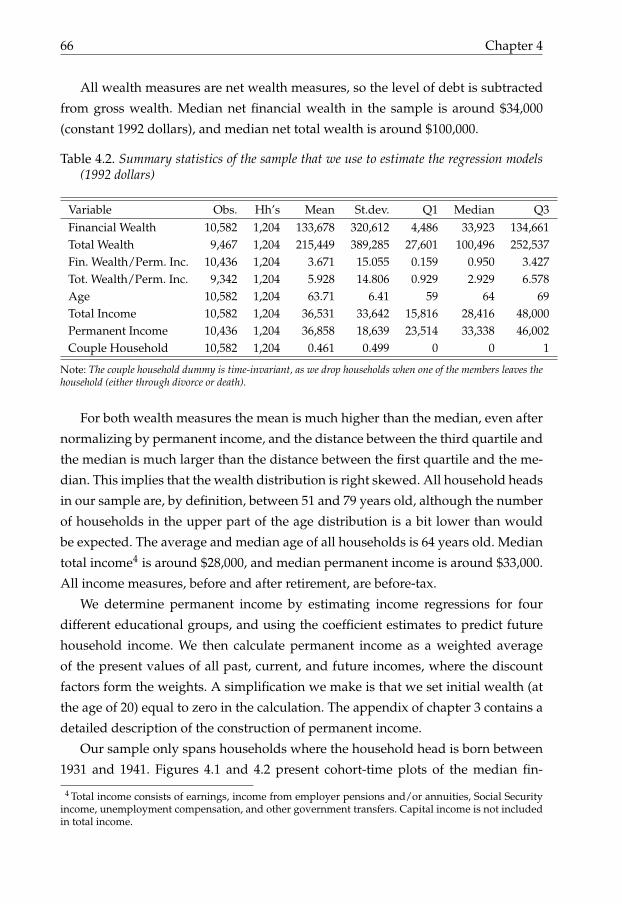
66 Chapter 4
All wealth measures are net wealth measures, so the level of debt is subtracted
from gross wealth. Median net financial wealth in the sample is around $34,000
(constant 1992 dollars), and median net total wealth is around $100,000.
Table 4.2. Summary statistics of the sample that we use to estimate the regression models(1992 dollars)
Variable Obs. Hh’s Mean St.dev. Q1 Median Q3Financial Wealth 10,582 1,204 133,678 320,612 4,486 33,923 134,661Total Wealth 9,467 1,204 215,449 389,285 27,601 100,496 252,537Fin. Wealth/Perm. Inc. 10,436 1,204 3.671 15.055 0.159 0.950 3.427Tot. Wealth/Perm. Inc. 9,342 1,204 5.928 14.806 0.929 2.929 6.578Age 10,582 1,204 63.71 6.41 59 64 69Total Income 10,582 1,204 36,531 33,642 15,816 28,416 48,000Permanent Income 10,436 1,204 36,858 18,639 23,514 33,338 46,002Couple Household 10,582 1,204 0.461 0.499 0 0 1
Note: The couple household dummy is time-invariant, as we drop households when one of the members leaves thehousehold (either through divorce or death).
For both wealth measures the mean is much higher than the median, even after
normalizing by permanent income, and the distance between the third quartile and
the median is much larger than the distance between the first quartile and the me-
dian. This implies that the wealth distribution is right skewed. All household heads
in our sample are, by definition, between 51 and 79 years old, although the number
of households in the upper part of the age distribution is a bit lower than would
be expected. The average and median age of all households is 64 years old. Median
total income4 is around $28,000, and median permanent income is around $33,000.
All income measures, before and after retirement, are before-tax.
We determine permanent income by estimating income regressions for four
different educational groups, and using the coefficient estimates to predict future
household income. We then calculate permanent income as a weighted average
of the present values of all past, current, and future incomes, where the discount
factors form the weights. A simplification we make is that we set initial wealth (at
the age of 20) equal to zero in the calculation. The appendix of chapter 3 contains a
detailed description of the construction of permanent income.
Our sample only spans households where the household head is born between
1931 and 1941. Figures 4.1 and 4.2 present cohort-time plots of the median fin-
4 Total income consists of earnings, income from employer pensions and/or annuities, Social Securityincome, unemployment compensation, and other government transfers. Capital income is not includedin total income.

Retirement replacement rates and saving behavior 67
ancial wealth/permanent income and median total wealth/permanent income ra-
tios. Note that productivity-related cohort effects are not present anymore in these
pictures, as wealth is divided by permanent income. Cohort1930 consists of house-
holds born before 1933, cohort1934 of households born in 1933, 1934, 1935, or 1936,
cohort1938 of households born in 1937, 1938, 1939, or 1940, and cohort1942 of house-
holds born after 1940. Only households from this last cohort clearly have higher
levels of wealth than households from the other three cohorts.
0.3
.6.9
1.2
1.5
1.8
2.1
finan
cial
wea
lth/p
erm
anen
t inc
ome
51 55 59 63 67 71 75 79age
cohort_1930 cohort_1934cohort_1938 cohort_1942
Figure 4.1. Median financial wealth/permanent income across age and cohorts
Less than half of all households in the sample are couple households. This seems
to be much lower than for the overall population between 50 and 80 years old.
The most obvious explanation is that it is easier to calculate a replacement rate for
single households; we just dropped a larger fraction of couple households from the
sample, as we were not able to calculate a replacement rate for them (see chapter 3
for details).

68 Chapter 4
0.6
1.2
1.8
2.4
33.
64.
24.
8to
tal w
ealth
/per
man
ent i
ncom
e
51 55 59 63 67 71 75 79age
cohort_1930 cohort_1934cohort_1938 cohort_1942
Figure 4.2. Median total wealth/permanent income across age and cohorts
4.3 Identification and Empirical Model
Our econometric specification to test the effect of the replacement rate on wealth
holdings is as follows:
Wht
YPh
= γ0 + γa + γt + γ1 log(RRh) + X′ht β + ϵht, (4.1)
where Wht is net wealth of household h in year t, YP is permanent income, γ0 is
a constant, γa captures the age effect, γt captures the time effect, RRh is the re-
placement rate of household h, and X is a vector of control variables, consisting
of education dummies, a dummy for couple households, sector dummies, and re-
gion dummies. Finally, ϵht is an error term, where we allow for intra-household
correlation, so all standard errors that we calculate are clustered at the level of the
household.
In a life cycle model with quadratic utility, all productivity-related cohort effects
are captured in the dependent variable, through their effect on permanent income
(see e.g. Kapteyn et al. (2005)). However, the above specification does not control for

Retirement replacement rates and saving behavior 69
other causes of cohort differences in wealth. For example, generations raised during
the Great Depression might be thriftier than other generations, and therefore have
higher levels of wealth. As the coefficients of a model with age-, time-, and cohort
dummies are unidentified, we choose to only include age- and time dummies in
the main specification.
There are three sources of endogeneity in equation 4.1. First, unobservable tastes
for saving might influence both the replacement rate and the level of wealth. This
is an example of omitted variable bias. Second, Coile and Gruber (2007) find that
retirement decisions are sensitive to the level of retirement wealth already accrued.
Thus, the level of wealth could affect the timing of retirement, which in turn de-
termines the replacement rate. In that case, correlation between the error term and
the replacement rate is caused by simultaneity. Finally, pension income as well as
earnings are most likely measured with error. The replacement rate is obtained by
taking the ratio of these two variables, so the replacement rate will suffer from
measurement error.
If thrifty individuals choose jobs based on generous pension arrangements, the
effect of the replacement rate on wealth levels would be biased upwards. On the
other hand, if wealthy individuals decide to retire earlier, because they can afford
so, the effect would be biased downwards. In the displacement literature, measure-
ment error causes a negative correlation between the wealth/permanent income
ratio and pension wealth, the main independent variable, because measurement er-
ror in pension wealth and permanent income are positively related. In our model,
however, the replacement rate is a ratio of two variables that together determine
permanent income. We thus believe that the correlation between measurement er-
ror in permanent income and measurement error in our main independent variable
is not as problematic as in the displacement literature. However, general measure-
ment error in the replacement rate might cause attenuation bias, which would drive
the coefficient estimate towards zero.
In order to overcome the endogeneity problem we use an instrument for the
replacement rate. We construct this instrument from the data itself. By calculating
median replacement rates over census regions and job sectors, we are able to as-
sign a so-called ”potential replacement rate” to each household, which can be used
as an instrument for the replacement rate. As long as workers do not sort across
employment sectors and do not move to a different census region in search of jobs
with more generous pension arrangements, the instrument is exogenous. Note that
these assumptions are also made by, among others, Attanasio and Brugiavini (2003)

70 Chapter 4
and Engelhardt and Kumar (2011).
The first source of variation in our instrument is thus the census region a house-
hold is living. This effect runs through the timing of retirement. Munnell et al. (2008)
show that there are considerable differences in labor participation rates of men aged
55-64 across states and census regions. Especially in the regions East South Central
and South Atlantic the labor participation rate of older men is low, compared to the
rest of the country. In the regions West North Central, and New England, on the
other hand, the labor participation rate of this group of men is significantly higher
than in the rest of the country. Also, Coile and Gruber (2007) report that early retire-
ment is significantly more prevalent in the Pacific region, and significantly less in
New England, compared to the other regions of the country. Early retirement will,
ceteris paribus, decrease the replacement rate, as workers simply have had less time
to accumulate pension savings. Also, Social Security benefits are lower when they
are claimed before the official retirement age. Munnell et al. (2008) show that, after
controlling for individual worker characteristics, state- or region-specific labor mar-
ket conditions are important in determining these differences in labor participation
rates of individuals around retirement.
The second source of variation is the sector where the household head has had
his or her job with longest reported tenure. We divide the economy in four sectors:
the primary sector, the secondary sector, the tertiary sector, and the public sector.
The generosity of pension schemes differs widely among sectors. For example, it
is well known that pension arrangements in the public sector are generally very
good compared to the private sector. Although the replacement rate of Social Se-
curity (first pillar) is mainly determined by the level of pre-retirement income (it
is decreasing in earnings), the extent to which employer-provided pension plans
(second pillar, together with 401(k)) meet the need of a reasonable standard of liv-
ing after retirement depends, among other things, on the sector in which the worker
is employed.
The variation in our instrument will thus be independent of individual char-
acteristics that cause the endogeneity of the replacement rate. Table 4.3 presents
median replacement rates for all 9 census regions and 4 employment sectors:
The median RRO is highest in census region West North Central, which is in line
with the evidence of Munnell et al. (2008) that labor participation rates of older men
are relatively high in this region. The regions West South Central and Mountain
have the lowest median RRO, while New England has the lowest median RRFP.
This is most probably due to the relatively high income level in New England. As

Retirement replacement rates and saving behavior 71
Table 4.3. Median values RRFP and RRO per census region and per sector
Census region Obs. RRFP RRO Sector Obs. RRFP RRO
New England 410 0.28 0.45 Primary Sector 336 0.40 0.46Mid Atlantic 1,576 0.30 0.51 Secondary Sector 3,584 0.37 0.46East North Central 1,653 0.31 0.49 Tertiary Sector 5,884 0.31 0.51West North Central 1,058 0.37 0.55 Public Sector 572 0.26 0.54South Atlantic 2,679 0.35 0.48East South Central 744 0.38 0.48West South Central 832 0.33 0.41Mountain 485 0.31 0.44Pacific 1,120 0.30 0.51p-value median test 0.000 0.000 0.000 0.000
expected, the employment sector ”Public Sector” has the highest median RRO, and
the lowest RRFP. The median tests at the bottom of the table show that there are
significant differences between sectors and regions for both RRFP and RRO.
To account for the endogeneity of the replacement rate in equation 4.1 we em-
ploy the instrumental variable quantile regression (IVQR) estimator of Chernozhukov
and Hansen (2008)5. The first stage is estimated by OLS, and the second stage by
quantile regression. We limit ourselves to the 50th percentile, essentially performing
median regressions.
An alternative to quantile regression would be to take the log of wealth, as
wealth is more or less lognormally distributed. However, around 11% of observa-
tions concern non-positive wealth levels, so they would be lost after a logarithmic
transformation of the data. It is hard to maintain that this is a random part of the
wealth distribution. The sample would become biased towards households with
positive wealth holdings. Furthermore, quantile regression is more robust against
influential outliers (Koenker, 2005).
4.4 Results
We show results in this section. First, we present findings of estimating the baseline
model. Second, we split our sample into four groups based on the distribution of
the replacement rate, and estimate an age-wealth profile for each of the four groups
separately. Finally, we perform robustness checks.
5 The Matlab file that we use comes from the website of Christian Hansen:http://faculty.chicagobooth.edu/christian.hansen/research/

72 Chapter 4
4.4.1 Baseline Specification
Table 4.4 presents results from estimating equation 4.1 by quantile regression (QR)
and instrumental variable quantile regression (IVQR). The first two columns con-
tain results for RRFP, and the last two columns for RRO. The quantile regression
in the first column shows an estimate of -0.160 for the effect of log RRFP on the
financial wealth/permanent income ratio. This would imply that a 10% increase
in the replacement rate is associated with a fall in the financial wealth/permanent
income ratio of about 0.016. The interpretation is that the difference in average life-
time wealth would be $640 between two households with a permanent income of
$40,000 that are equal to each other in all other respects, except that the household
with the higher level of wealth has a 10% lower replacement rate.
Using the IVQR estimator, we find an insignificant estimate of log RRFP of -
0.065. Apparently, endogeneity leads to a downward bias of the estimate because
taking it into account gives an estimate very close to (and insignificant from) zero.
These results suggest that general measurement error can not be the only cause of
the endogeneity, because if that would have been the case the QR estimate would
have been closer to zero than the IVQR estimate, which is not the case. The coef-
ficient on the instrument in the first stage equals 0.715 and is strongly significant.
Furthermore, the partial F-statistic is 12.6. Note that the life cycle model predicts
that the age-wealth profile of households with a high replacement rate lies below
the profile of households with a low replacement rate. However, it also predicts
that the distance between the two profiles is largest around retirement. We will
come back to this in the next subsection.
Using RRO the estimates are -0.120 and -0.052, but the latter estimate is in-
significantly different from zero. However, as Engelhardt and Kumar (2011) and
Chernozhukov and Hansen (2008) also note, the IVQR estimator is very inefficient.
Although the quantile regression estimates are negative and significant, the IVQR
estimates are insignificant, so we cannot conclude that there is a negative correl-
ation between the replacement rate and the financial wealth/permanent income
ratio. Note also that the partial F-statistic of 6.3 indicates a weak instrument prob-
lem. Finally, the education dummies and the couple household dummy have the
expected positive signs and are all strongly significant.
Adding housing wealth to financial wealth gives total wealth. It is interesting
to examine whether the results for total wealth are comparable to financial wealth
as housing wealth is one of the most illiquid forms of wealth. We therefore think
that, in the context of the life cycle model, it is appropriate to treat it in a different
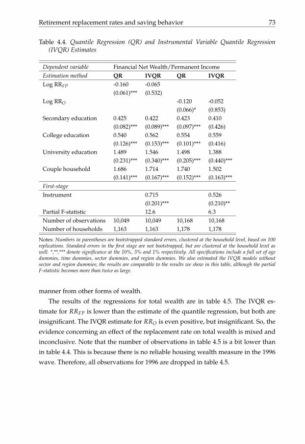
Retirement replacement rates and saving behavior 73
Table 4.4. Quantile Regression (QR) and Instrumental Variable Quantile Regression(IVQR) Estimates
Dependent variable Financial Net Wealth/Permanent IncomeEstimation method QR IVQR QR IVQRLog RRFP -0.160 -0.065
(0.061)*** (0.532)Log RRO -0.120 -0.052
(0.066)* (0.853)Secondary education 0.425 0.422 0.423 0.410
(0.082)*** (0.089)*** (0.097)*** (0.426)College education 0.540 0.562 0.554 0.559
(0.126)*** (0.153)*** (0.101)*** (0.416)University education 1.489 1.546 1.498 1.388
(0.231)*** (0.340)*** (0.205)*** (0.440)***Couple household 1.686 1.714 1.740 1.502
(0.141)*** (0.167)*** (0.152)*** (0.163)***First-stageInstrument 0.715 0.526
(0.201)*** (0.210)**Partial F-statistic 12.6 6.3Number of observations 10,049 10,049 10,168 10,168Number of households 1,163 1,163 1,178 1,178
Notes: Numbers in parentheses are bootstrapped standard errors, clustered at the household level, based on 100replications. Standard errors in the first stage are not bootstrapped, but are clustered at the household level aswell. *,**,*** denote significance at the 10%, 5% and 1% respectively. All specifications include a full set of agedummies, time dummies, sector dummies, and region dummies. We also estimated the IVQR models withoutsector and region dummies; the results are comparable to the results we show in this table, although the partialF-statistic becomes more than twice as large.
manner from other forms of wealth.
The results of the regressions for total wealth are in table 4.5. The IVQR es-
timate for RRFP is lower than the estimate of the quantile regression, but both are
insignificant. The IVQR estimate for RRO is even positive, but insignificant. So, the
evidence concerning an effect of the replacement rate on total wealth is mixed and
inconclusive. Note that the number of observations in table 4.5 is a bit lower than
in table 4.4. This is because there is no reliable housing wealth measure in the 1996
wave. Therefore, all observations for 1996 are dropped in table 4.5.

74 Chapter 4
Table 4.5. Quantile Regression (QR) and Instrumental Variable Quantile Regression(IVQR) Estimates
Dependent variable Total Net Wealth/Permanent IncomeEstimation method QR IVQR QR IVQRLog RRFP -0.249 -0.483
(0.169) (1.460)Log RRO -0.342 0.431
(0.195)* (1.205)Secondary education 0.916 0.877 0.965 0.991
(0.185)*** (0.271)*** (0.189)*** (0.498)**College education 1.094 1.055 1.175 1.242
(0.238)*** (0.541)* (0.232)*** (0.496)**University education 2.400 2.268 2.506 2.609
(0.431)*** (0.933)** (0.362)*** (0.759)***Couple household 3.405 3.358 3.439 3.430
(0.262)*** (0.323)*** (0.243)*** (0.261)***First-stageInstrument 0.715 0.527
(0.199)*** (0.211)**Partial F-statistic 12.9 6.3Number of observations 8,996 8,996 9,101 9,101Number of households 1,163 1,163 1,178 1,178
Notes: Numbers in parentheses are bootstrapped standard errors, clustered at the household level, based on 100replications. Standard errors in the first stage are not bootstrapped, but are clustered at the household level aswell. *,**,*** denote significance at the 10%, 5% and 1% respectively. All specifications include a full set of agedummies, time dummies, sector dummies, and region dummies. We also estimated the IVQR models withoutsector and region dummies; the results are comparable to the results we show in this table, although the partialF-statistic becomes more than twice as large.
4.4.2 Age-Wealth Profiles
As already noted, if households behave according to the life cycle model the age-
wealth profile of households with a high replacement rate should lie below the pro-
file of households with a low replacement rate. Furthermore, the distance between
the profiles should be at its maximum around retirement. Households with a low
replacement rate should save more before retirement, and dissave more after re-
tirement, so their age-wealth profile is expected to be steeper than the profile of
households with a high replacement rate.
We divide the sample into four subsamples, based on the distribution of the
replacement rate. However, due to the endogeneity of the replacement rate, we
cannot simply use the data to define the quartiles. Therefore, we first estimate the

Retirement replacement rates and saving behavior 75
first stage and base the quartiles on the distribution of the predicted replacement
rate, instead of the actual values of the replacement rate. We then estimate quantile
regressions for each of the four subsamples, and examine the resulting age-wealth
profiles. The estimation procedure consists thus of two steps:
1. OLS regression of the endogenous variable, the (log) replacement rate, on the
exogenous variables and the instrument. Based on the regression estimates,
we calculate fitted values and define the four quartiles of the predicted re-
placement rate.
2. Quantile regressions for each of the four samples, with the ratio of wealth to
permanent income regressed on the exogenous variables.
Table 4.6 presents the estimation results for financial wealth. The first four columns
contain results for RRFP, and the last four columns for RRO. Instead of age dum-
mies, we have defined a linear spline in age such that each spline contains an equal
amount of observations. As the sample size of each regression is four times as small
as in tables 4.4 and 4.5 the model would become overparameterized with age dum-
mies. Furthermore, we have excluded education dummies, region dummies, and
sector dummies to limit convergence problems while estimating the model.
The coefficient estimate of the couple household dummy is in line with the find-
ings in tables 4.4 and 4.5. We also show the coefficient estimates for all age spline
variables. Figures 4.3 and 4.4 show age-wealth profiles for all four quartiles of the
replacement rate distribution, based on these coefficient estimates. The other vari-
ables are evaluated at their sample means.
Figure 4.3 reveals that the amount of wealth that is accumulated before retire-
ment is decreasing in RRFP. Households from the lowest quartile of the replace-
ment rate-distribution have accumulated six times as much financial wealth, rel-
ative to permanent income, around the age of 65 than households in the highest
quartile of the distribution. This is in line with the predictions of the life cycle
model. The picture of wealth decumulation after retirement is less clear, which is
partly caused by the large standard errors of the estimates of age 70-79. However,
it seems that households in the highest two quartiles of the distribution, so with
the highest RRFP’s, do not dissave after retirement. This is again what the life cycle
model predicts.
Households with a lower RRFP keep saving after retirement. Possible explan-
ations might be uncertain life expectancies and the risk of out-of-pocket medical
expenses for these households (see De Nardi et al. (2009, 2010)). In addition, sev-

76 Chapter 4
−1
01
23
45
fin. w
ealth
/per
m. i
ncom
e
50 60 70 80age
first quartile
−1
01
23
45
fin. w
ealth
/per
m. i
ncom
e
50 60 70 80age
second quartile
−1
01
23
45
fin. w
ealth
/per
m. i
ncom
e
50 60 70 80age
third quartile
−1
01
23
45
fin. w
ealth
/per
m. i
ncom
e
50 60 70 80age
fourth quartile
Figure 4.3. Age-financial wealth profiles (solid lines) for all quartiles of the RRFP-distribution. The dashed lines represent 95% confidence bounds, based on 1000bootstrap replications (clustered at the household level).
eral studies have documented that households experience a drop in consumption
around retirement (e.g., Banks et al. (1998), Bernheim et al. (2001), Haider and
Stephens (2007)). This could also explain why households do not dissave after re-
tirement, namely that they simply do not need to as their pension income is high
enough to satisfy their consumption needs.
The age-wealth profiles in figure 4.4, where the quartiles of the RRO-distribution
are used, are comparable to the ones in figure 4.3. Again, in none of the four groups
households decumulate wealth after retirement, while the accumulation of wealth
before retirement is decreasing in the replacement rate.
If we include housing wealth the picture roughly stays the same, as table 4.7
and figures 4.5 and 4.6 reveal. If there is any wealth decumulation at all, it is in the
lowest quartiles of the replacement rate distribution. Furthermore, also total wealth
is decreasing in the replacement rate.

Retirement replacement rates and saving behavior 77
−1
01
23
45
fin. w
ealth
/per
m. i
ncom
e
50 60 70 80age
first quartile
−1
01
23
45
fin. w
ealth
/per
m. i
ncom
e
50 60 70 80age
second quartile
−1
01
23
45
fin. w
ealth
/per
m. i
ncom
e
50 60 70 80age
third quartile
−1
01
23
45
fin. w
ealth
/per
m. i
ncom
e
50 60 70 80age
fourth quartile
Figure 4.4. Age-financial wealth profiles (solid lines) for all quartiles of the RRO-distribution. The dashed lines represent 95% confidence bounds, based on 1000bootstrap replications (clustered at the household level).
4.4.3 Robustness Checks
To check the influence of accounting for the endogeneity of the replacement rate on
our findings, we perform a robustness check. Instead of dividing the sample in four
parts based on the distribution of the fitted values of a regression with the replace-
ment rate as left-hand side variable, we divide the sample in four parts based on
the actual distribution of the replacement rate. We thus treat the replacement rate
as an exogenous variable. Tables 4.8 and 4.9 present the regression results for the
four groups, and figures 4.7-4.10 show the age-wealth profiles that these regression
results imply.
The main difference with the baseline results is that when we divide the sample
on the basis of actual replacement rates, households in the lowest two quartiles of
the RRFP distribution decumulate wealth after retirement, while these groups keep
accumulating wealth in the baseline model. Of course, the nature of the robustness
check implies that the composition of these groups differs. However, in general we
observe the same patterns as in figures 4.3-4.6: Wealth accumulation is decreasing
in the replacement rate and there is hardly decumulation of wealth after retirement.

78 Chapter 4
−1
37
1115
tota
l wea
lth/p
erm
. inc
ome
50 60 70 80age
first quartile
−1
37
1115
tota
l wea
lth/p
erm
. inc
ome
50 60 70 80age
second quartile
−1
37
1115
tota
l wea
lth/p
erm
. inc
ome
50 60 70 80age
third quartile
−1
37
1115
tota
l wea
lth/p
erm
. inc
ome
50 60 70 80age
fourth quartile
Figure 4.5. Age-total wealth profiles (solid lines) for all quartiles of the RRFP-distribution. The dashed lines represent 95% confidence bounds, based on 1000bootstrap replications (clustered at the household level).

Retirement replacement rates and saving behavior 79
Tabl
e4.
6.Q
uant
ileR
egre
ssio
nsw
ithSu
bsam
ples
Base
don
the
Rep
lace
men
tRat
e-D
istr
ibut
ion
Dep
ende
ntva
riab
leFi
nanc
ialN
etW
ealt
h/Pe
rman
entI
ncom
eR
epla
cem
entr
ate
RR
FPR
RO
Qua
rtile
repl
acem
entr
ate-
dist
r.1s
t2n
d3r
d4t
h1s
t2n
d3r
d4t
hA
ge51
-58
0.07
80.
085
0.04
80.
020
0.10
30.
069
0.04
20.
030
(0.0
38)*
*(0
.038
)**
(0.0
29)*
(0.0
11)*
(0.0
44)*
*(0
.028
)**
(0.0
30)
(0.0
18)
Age
58-6
20.
159
0.09
60.
066
0.03
90.
080
0.12
30.
119
0.04
1(0
.068
)**
(0.0
67)
(0.0
59)
(0.0
21)*
(0.0
68)
(0.0
48)*
*(0
.048
)**
(0.0
27)
Age
62-6
60.
087
0.19
90.
004
0.03
20.
082
0.05
70.
084
0.03
6(0
.085
)(0
.064
)***
(0.0
44)
(0.0
18)*
(0.0
75)
(0.0
56)
(0.0
50)*
(0.0
30)
Age
66-7
0-0
.168
0.07
5-0
.070
0.00
90.
019
-0.0
23-0
.002
0.02
2(0
.081
)**
(0.0
55)
(0.0
43)*
(0.0
15)
(0.0
67)
(0.0
46)
(0.0
43)
(0.0
22)
Age
70-7
90.
138
0.04
8-0
.001
0.00
20.
086
0.02
70.
039
-0.0
06(0
.098
)(0
.056
)(0
.026
)(0
.012
)(0
.070
)(0
.046
)(0
.042
)(0
.016
)C
oupl
eho
useh
old
2.44
72.
110
1.46
90.
773
2.15
62.
101
1.74
01.
513
(0.3
58)*
**(0
.223
)***
(0.2
64)*
**(0
.182
)***
(0.2
43)*
**(0
.341
)***
(0.2
62)*
**(0
.370
)***
Num
ber
ofob
serv
atio
ns2,
556
2,56
12,
569
2,52
42,
558
2,55
62,
553
2,54
3N
umbe
rof
hous
ehol
ds32
135
936
832
637
142
641
636
2
Not
es:N
umbe
rsin
pare
nthe
ses
are
boot
stra
pped
stan
dard
erro
rs,c
lust
ered
atth
eho
useh
old
leve
l,ba
sed
on10
0re
plic
atio
ns.*
,**,
***
deno
tesi
gnifi
canc
eat
the
10%
,5%
and
1%re
spec
tivel
y.In
the
first
step
the
endo
geno
usva
riab
les,
(log)
RR
FPan
d(lo
g)R
RO
are
regr
esse
don
the
exog
enou
sva
riab
les
and
the
inst
rum
ent.
Base
don
the
regr
essi
ones
timat
es,
wec
alcu
late
fitte
dva
lues
and
defin
ethe
four
quar
tiles
ofth
epre
dict
edR
RFP
and
RR
O.I
nth
esec
ond
step
wep
erfo
rmqu
antil
ereg
ress
ions
fore
ach
ofth
efou
rsub
sam
ples
,with
the
ratio
ofw
ealth
tope
rman
enti
ncom
ere
gres
sed
onth
eex
ogen
ous
vari
able
s.A
llsp
ecifi
catio
nsin
clud
ea
full
seto
ftim
edu
mm
ies.
The
age
effe
cts
are
capt
ured
bya
linea
rsp
line
inag
e.Ed
ucat
ion
dum
mie
s,re
gion
dum
mie
s,an
dse
ctor
dum
mie
sar
eex
clud
edin
the
quan
tile
regr
essi
ons
tolim
itco
nver
genc
epr
oble
ms,
butn
ote
that
thes
edu
mm
ies
are
incl
uded
tode
term
ine
the
dist
ribu
tion
ofth
ere
plac
emen
tra
tein
the
first
step
.We
also
estim
ated
alls
peci
ficat
ions
with
adu
mm
yfo
rco
hort
1942
incl
uded
(see
sect
ion
2).H
owev
er,t
heco
effic
ient
estim
ate
isin
sign
ifica
ntin
alls
peci
ficat
ions
and
the
estim
ates
ofth
eot
her
coef
ficie
nts
are
com
para
ble
toth
eon
esin
this
tabl
e.

80 Chapter 4
Tabl
e4.
7.Q
uant
ileR
egre
ssio
nsw
ithSu
bsam
ples
Base
don
the
Rep
lace
men
tRat
e-D
istr
ibut
ion
Dep
ende
ntva
riab
leTo
talN
etW
ealt
h/Pe
rman
entI
ncom
eR
epla
cem
entr
ate
RR
FPR
RO
Qua
rtile
repl
acem
entr
ate-
dist
r.1s
t2n
d3r
d4t
h1s
t2n
d3r
d4t
hA
ge51
-58
0.15
20.
198
0.20
20.
081
0.24
10.
181
0.05
10.
151
(0.0
80)*
*(0
.063
)***
(0.0
50)*
**(0
.064
)(0
.053
)***
(0.0
67)*
**(0
.084
)(0
.039
)***
Age
58-6
20.
157
0.05
20.
127
0.20
00.
138
0.09
80.
098
0.20
4(0
.113
)(0
.089
)(0
.090
)(0
.054
)***
(0.1
36)
(0.1
00)
(0.0
79)
(0.0
76)*
**A
ge62
-66
0.06
90.
196
0.17
90.
013
0.16
10.
203
0.10
80.
133
(0.1
20)
(0.1
19)*
(0.1
09)
(0.0
48)
(0.1
53)
(0.1
24)
(0.0
89)
(0.0
70)*
Age
66-7
0-0
.065
0.07
1-0
.171
-0.0
040.
087
-0.1
86-0
.028
0.07
1(0
.167
)(0
.107
)(0
.107
)(0
.078
)(0
.145
)(0
.109
)*(0
.105
)(0
.075
)A
ge70
-79
0.18
60.
054
0.07
3-0
.013
0.03
80.
045
-0.0
120.
120
(0.1
90)
(0.1
17)
(0.0
72)
(0.0
62)
(0.1
48)
(0.1
39)
(0.0
78)
(0.0
86)
Cou
ple
hous
ehol
d3.
832
3.65
72.
919
3.14
43.
674
3.68
43.
141
3.58
5(0
.558
)***
(0.4
20)*
**(0
.341
)***
(0.4
59)*
**(0
.447
)***
(0.4
65)*
**(0
.364
)***
(0.4
89)*
**N
umbe
rof
obse
rvat
ions
2,27
82,
295
2,29
42,
271
2,29
62,
290
2,27
92,
273
Num
ber
ofho
useh
olds
328
359
368
326
371
424
415
358
Not
es:S
eeta
ble
4.6

Retirement replacement rates and saving behavior 81
−1
37
1115
tota
l wea
lth/p
erm
. inc
ome
50 60 70 80age
first quartile
−1
37
1115
tota
l wea
lth/p
erm
. inc
ome
50 60 70 80age
second quartile
−1
37
1115
tota
l wea
lth/p
erm
. inc
ome
50 60 70 80age
third quartile
−1
37
1115
tota
l wea
lth/p
erm
. inc
ome
50 60 70 80age
fourth quartile
Figure 4.6. Age-total wealth profiles (solid lines) for all quartiles of the RRO-distribution. The dashed lines represent 95% confidence bounds, based on 1000bootstrap replications (clustered at the household level).

82 Chapter 4
Tabl
e4.
8.Q
uant
ileR
egre
ssio
nsw
ithSu
bsam
ples
Base
don
the
Rep
lace
men
tRat
e-D
istr
ibut
ion
Dep
ende
ntva
riab
leFi
nanc
ialN
etW
ealt
h/Pe
rman
entI
ncom
eR
epla
cem
entr
ate
RR
FPR
RO
Qua
rtile
repl
acem
entr
ate-
dist
r.1s
t2n
d3r
d4t
h1s
t2n
d3r
d4t
hA
ge51
-58
0.06
80.
079
0.03
20.
006
0.06
70.
029
0.02
60.
035
(0.0
38)*
(0.0
28)*
**(0
.028
)(0
.016
)(0
.034
)**
(0.0
26)
(0.0
24)
(0.0
26)
Age
58-6
20.
102
0.04
90.
018
0.05
50.
121
0.10
30.
049
0.02
4(0
.057
)*(0
.050
)(0
.044
)(0
.024
)**
(0.0
58)*
*(0
.043
)**
(0.0
49)
(0.0
31)
Age
62-6
6-0
.097
0.13
2-0
.003
0.06
00.
056
-0.0
390.
071
0.08
8(0
.085
)(0
.066
)**
(0.0
45)
(0.0
30)*
*(0
.068
)(0
.040
)(0
.054
)(0
.039
)**
Age
66-7
0-0
.078
-0.0
53-0
.067
0.00
4-0
.015
-0.0
30-0
.080
0.01
0(0
.077
)(0
.057
)(0
.044
)(0
.016
)(0
.060
)(0
.039
)(0
.040
)**
(0.0
33)
Age
70-7
9-0
.078
-0.0
20-0
.002
0.02
90.
083
-0.0
11-0
.030
0.05
7(0
.051
)(0
.047
)(0
.035
)(0
.021
)(0
.058
)(0
.032
)(0
.023
)(0
.030
)*C
oupl
eho
useh
old
2.60
22.
423
1.09
20.
892
3.26
31.
792
1.83
21.
323
(0.3
45)*
**(0
.312
)***
(0.2
25)*
**(0
.242
)***
(0.4
25)*
**(0
.250
)***
(0.2
82)*
**(0
.267
)***
Num
ber
ofob
serv
atio
ns2,
580
2,56
92,
575
2,55
12,
596
2,29
22,
275
2,27
4N
umbe
rof
hous
ehol
ds29
929
029
329
930
329
829
829
7
Not
es:N
umbe
rsin
pare
nthe
ses
are
boot
stra
pped
stan
dard
erro
rs,c
lust
ered
atth
eho
useh
old
leve
l,ba
sed
on10
0re
plic
atio
ns.*
,**,
***
deno
tesi
gnifi
canc
eat
the
10%
,5%
and
1%re
spec
tivel
y.W
edi
vide
the
sam
ple
into
four
quar
tiles
,bas
edon
the
dist
ribu
tion
ofR
RFP
and
RR
O.W
epe
rfor
mqu
antil
ere
gres
sion
sfo
rea
chof
the
subs
ampl
es,w
ithth
era
tioof
wea
lthto
perm
anen
tin
com
ere
gres
sed
onth
eex
ogen
ous
vari
able
s.A
llsp
ecifi
catio
nsin
clud
ea
full
set
oftim
edu
mm
ies.
The
age
effe
cts
are
capt
ured
bya
linea
rsp
line
inag
e.Ed
ucat
ion
dum
mie
s,re
gion
dum
mie
s,an
dse
ctor
dum
mie
sar
eex
clud
edin
the
quan
tile
regr
essi
ons
tolim
itco
nver
genc
epr
oble
ms.
Not
eth
atpo
ssib
leen
doge
neity
ofth
ere
plac
emen
trat
eis
fully
igno
red
inth
ese
regr
essi
ons.
We
also
estim
ated
alls
peci
ficat
ions
with
adu
mm
yfo
rco
hort
1942
incl
uded
(see
sect
ion
2).H
owev
er,t
heco
effic
ient
estim
ate
isin
sign
ifica
ntin
alls
peci
ficat
ions
and
the
estim
ates
ofth
eot
her
coef
ficie
nts
are
com
para
ble
toth
eon
esin
this
tabl
e.

Retirement replacement rates and saving behavior 83
Tabl
e4.
9.Q
uant
ileR
egre
ssio
nsw
ithSu
bsam
ples
Base
don
the
Rep
lace
men
tRat
e-D
istr
ibut
ion
Dep
ende
ntva
riab
leTo
talN
etW
ealt
h/Pe
rman
entI
ncom
eR
epla
cem
entr
ate
RR
FPR
RO
Qua
rtile
repl
acem
entr
ate-
dist
r.1s
t2n
d3r
d4t
h1s
t2n
d3r
d4t
hA
ge51
-58
0.04
40.
225
0.04
70.
129
0.18
70.
153
0.09
90.
126
(0.0
79)
(0.0
56)*
**(0
.055
)(0
.048
)***
(0.0
60)*
**(0
.055
)***
(0.0
69)
(0.0
44)*
**A
ge58
-62
0.11
00.
011
0.06
90.
155
0.09
10.
184
0.04
80.
102
(0.0
97)
(0.0
92)
(0.0
67)
(0.0
69)*
*(0
.106
)(0
.082
)**
(0.0
84)
(0.0
74)
Age
62-6
6-0
.075
0.11
30.
068
0.14
80.
034
0.02
00.
091
0.17
0(0
.121
)(0
.108
)(0
.089
)(0
.099
)(0
.124
)(0
.083
)(0
.084
)(0
.095
)*A
ge66
-70
-0.2
11-0
.107
-0.1
200.
016
-0.0
010.
025
-0.1
04-0
.042
(0.1
31)
(0.0
85)
(0.0
76)
(0.0
80)
(0.1
33)
(0.1
13)
(0.0
74)
(0.0
93)
Age
70-7
9-0
.175
-0.0
590.
049
0.16
4-0
.047
0.04
4-0
.147
0.14
8(0
.071
)**
(0.1
13)
(0.0
85)
(0.0
71)*
*(0
.141
)(0
.099
)(0
.061
)**
(0.0
60)*
*C
oupl
eho
useh
old
4.26
13.
392
2.68
03.
088
5.00
44.
001
3.08
42.
712
(0.5
82)*
**(0
.405
)***
(0.3
71)*
**(0
.359
)***
(0.6
82)*
**(0
.438
)***
(0.4
23)*
**(0
.353
)***
Num
ber
ofob
serv
atio
ns2,
310
2,29
92,
302
2,28
92,
330
2,32
32,
330
2,32
2N
umbe
rof
hous
ehol
ds29
929
029
329
930
329
829
829
7
Not
es:S
eeta
ble
4.8

84 Chapter 4
−1
01
23
45
fin. w
ealth
/per
m. i
ncom
e
50 60 70 80age
first quartile
−1
01
23
45
fin. w
ealth
/per
m. i
ncom
e
50 60 70 80age
second quartile
−1
01
23
45
fin. w
ealth
/per
m. i
ncom
e
50 60 70 80age
third quartile
−1
01
23
45
fin. w
ealth
/per
m. i
ncom
e
50 60 70 80age
fourth quartile
Figure 4.7. Age-financial wealth profiles (solid lines) for all quartiles of the RRFP-distribution. Note that possible endogeneity is ignored in determining this dis-tribution. The dashed lines represent 95% confidence bounds, based on 1000bootstrap replications (clustered at the household level).

Retirement replacement rates and saving behavior 85
−1
01
23
45
fin. w
ealth
/per
m. i
ncom
e
50 60 70 80age
first quartile
−1
01
23
45
fin. w
ealth
/per
m. i
ncom
e
50 60 70 80age
second quartile
−1
01
23
45
fin. w
ealth
/per
m. i
ncom
e
50 60 70 80age
third quartile
−1
01
23
45
fin. w
ealth
/per
m. i
ncom
e
50 60 70 80age
fourth quartile
Figure 4.8. Age-financial wealth profiles (solid lines) for all quartiles of the RRO-distribution. Note that possible endogeneity is ignored in determining this dis-tribution. The dashed lines represent 95% confidence bounds, based on 1000bootstrap replications (clustered at the household level).

86 Chapter 4
−1
37
1115
tota
l wea
lth/p
erm
. inc
ome
50 60 70 80age
first quartile
−1
37
1115
tota
l wea
lth/p
erm
. inc
ome
50 60 70 80age
second quartile
−1
37
1115
tota
l wea
lth/p
erm
. inc
ome
50 60 70 80age
third quartile
−1
37
1115
tota
l wea
lth/p
erm
. inc
ome
50 60 70 80age
fourth quartile
Figure 4.9. Age-total wealth profiles (solid lines) for all quartiles of the RRFP-distribution. Note that possible endogeneity is ignored in determining this dis-tribution. The dashed lines represent 95% confidence bounds, based on 1000bootstrap replications (clustered at the household level).

Retirement replacement rates and saving behavior 87
−1
37
1115
tota
l wea
lth/p
erm
. inc
ome
50 60 70 80age
first quartile
−1
37
1115
tota
l wea
lth/p
erm
. inc
ome
50 60 70 80age
second quartile
−1
37
1115
tota
l wea
lth/p
erm
. inc
ome
50 60 70 80age
third quartile
−1
37
1115
tota
l wea
lth/p
erm
. inc
ome
50 60 70 80age
fourth quartile
Figure 4.10. Age-total wealth profiles (solid lines) for all quartiles of the RRO-distribution. Note that possible endogeneity is ignored in determining this dis-tribution. The dashed lines represent 95% confidence bounds, based on 1000bootstrap replications (clustered at the household level).

88 Chapter 4
4.5 Conclusions
The finding that large groups of households keep saving after retirement is already
well-documented in the literature (see, among others, Alessie et al. (1997), Banks
and Rohwedder (2003)). We confirm this finding. However, we do not find sup-
port for the hypothesis that the amount of financial wealth is decreasing in the
retirement replacement rate. So, we are unable to claim a causal effect of the re-
placement rate on the amount of accumulated wealth. Whether this effect is simply
not there or the IVQR estimator is too inefficient remains an open question. Finally,
the age-wealth profile of households in the highest quartile of the replacement rate-
distribution is very flat, which is in line with the predictions of the life cycle model.
One of the limitations of our study is that we do not have access to inform-
ation about the state where households are living. Using this information would
make the instrument stronger, as the variation in replacement rates is much larger
between states than between census regions. Furthermore, data on the complete
income history of households would allow us to improve the caluculation of per-
manent income and the replacement rate. An interesting avenue for future research
would be to examine what the main determinants are of differences in replacement
rates. Also, the issues around the calculation of replacement rates deserve some
more attention.

Chapter 5
Funding of pensions and
economic growth: Are they
really related?
5.1 Introduction
In many countries pay-as-you-go (PAYG) pension systems are being replaced by
(partly) funded pension systems, a shift largely motivated by population aging.
Proponents of these shifts also argue that funded pension systems can lead to higher
economic growth. If this effect arises during the transition, it could partly allevi-
ate the transition burden associated with the shift from PAYG to funding (Borsch-
Supan et al., 2005). Considering the vast number of countries undertaking sim-
ilar transitions, it is useful to examine whether these shifts led to higher economic
growth rates.
A few empirical studies (Holzmann, 1997a,b, Davis and Hu, 2008) argue that
funding of pensions is associated with higher economic growth rates, due to higher
saving rates, capital market development and reduced labor market distortions. In
a PAYG system, pension contributions represent transfers from the young to the
old; in a funded pension system, the contributions can be viewed as savings. There-
fore, a higher degree of funding means more people save through their mandatory
pension scheme, which should lead to a higher aggregate saving rate. Capital mar-
ket development also could be stimulated because more resources become available
This chapter is based on Zandberg and Spierdijk (2013)

90 Chapter 5
for the capital market when pensions are funded. Finally, labor market distortions
might be mitigated, because funded pension systems have less distorting effects on
labor supply decisions than do unfunded systems. These three effects all suggest
higher growth.
Our evidence of an effect of funding on growth is mixed. For the short-run we
do not find any effect at all, while we find some evidence for an effect in the long-
run. However, this latter evidence highly depends on the empirical model that we
use. There seems to be a positive effect when we estimate a model with overlapping
observations, but we do not find this positive effect when we use a simple cross-
sectional model.
The data set we use spans 54 countries, 29 of which are OECD countries, during
the years 2001-2010. To examine whether changes in the degree of funding affect
economic growth in the short-run we estimate a dynamic growth model with the
growth rate of the ratio of pension assets over GDP as main explanatory variable.
We employ a bias-corrected Least Square Dummy Variable (LSDV)-estimator with
bootstrap standard errors where we assume country-specific steady-state growth
rates. The growth rate of pension assets is insignificant in all specifications, with
coefficient estimates that are very close to zero. We also estimate a model without
country fixed effects, and the results are comparable.
To find a possible long-run effect we use a simple cross-sectional growth model
and estimate it by OLS. Once we also include initial income, which has a negative
effect on growth as predicted by the convergence literature (see Barro (1997)), the
growth rate of pension assets becomes insignificant. However, when we estimate a
growth model with overlapping observations the growth rate of pension assets has
a significantly positive effect on economic growth, which remains after the inclu-
sion of initial income, although the coefficient estimates become smaller. We correct
the standard errors in the overlapping observations model for serial correlation that
is caused by the overlapping nature of the data.
Davis and Hu (2008) also examine empirically whether the level of pension as-
sets, scaled by GDP, is related to economic growth; they conclude that pension fund
growth is positively related to economic growth, especially in emerging market eco-
nomies. Holzmann (1997a,b) finds a positive relationship between pension reform
and total factor productivity in Chile, and Davis (2002, 2004) has examined the link
between institutionalization (i.e., the proportion of equity held by institutional in-
vestors) and GDP growth but finds no effect. However, these last two studies do not
test the hypothesis that pension funding increases economic growth, because they

Funding of pensions and economic growth 91
include insurance companies and mutual funds as part of institutional investors.
The rest of the chapter is organized as follows: In Section 2 we present the the-
ory. Then in Section 3, we describe the data, followed in Section 4 by a description
of the empirical strategy and the results. Finally, we conclude in Section 5.
5.2 Theory
In this section we consider the channels through which funding might influence
economic growth. We divide these into the effect through the aggregate saving rate,
which has received most attention in the literature, and other channels.
Pension systems can be funded, unfunded, or partly funded. In an unfunded
pension system, or PAYG system, the currently young pay taxes that are used to
pay pensions to the currently old in the same period. In a funded pension system,
young workers contribute to a pension fund and then receive pension benefits from
this fund when they retire. In a PAYG system, no pension assets exist, because the
contributions are immediately used to pay pension benefits; a funded system in-
stead has a pool of assets available. In most countries, pension systems combine
PAYG and funded elements, though worldwide trends indicate increased switch-
ing from PAYG to (partly) funded pension systems. This switch creates consider-
able transition costs, because the windfall gain for the first generation of pension
beneficiaries must be paid back implicitly (Sinn, 2000). Borsch-Supan et al. (2005)
argue however that such pension reforms lead to higher economic growth, because
they increase saving rates and the efficiency of capital markets, which partly com-
pensates for the transition costs. Furthermore, increased growth should alleviate
problems associated with an aging population, which are the primary motives for
reforming pension systems. These arguments suggest that funding of pensions can
increase economic growth rates by increasing the aggregate saving rate, develop-
ment of capital markets, reducing labor market distortions, and improving corpor-
ate governance.
5.2.1 Aggregate Saving Rate
The contributions of workers to a PAYG system represent a pure tax, because they
are used immediately to pay pension benefits to retirees. In contrast, the pension
premiums in a funded system constitute savings that get invested in the capital

92 Chapter 5
market. A shift toward more funding therefore might increase the aggregate saving
rate and, accordingly, may increase economic growth. For this effect to be operat-
ive in practice, three conditions must be fulfilled (Barr, 2000): Funding must lead to
a higher saving rate than PAYG, the additional savings must induce more invest-
ment, and additional investments must lead to a higher economic growth rate.
Although the effect of funding on saving could be permanent, it might be highest
during the transition from the PAYG system to the funded system. That is, during
the transition, funds build-up and this leads to a net increase in pension fund as-
sets. At some point in time though, the pension fund matures, and the net inflow
of funds slows or even becomes negative, such that the outflow of funds to pension
beneficiaries creates dissaving.
A few other issues may play a role as well. The transition to a funded system
must be financed by either the government or the workers. In the former case, the
government issues debt that might undo the possible positive effect on the aggreg-
ate saving rate. Furthermore, as Blanchard and Fischer (1989) point out, a funded
pension system can increase the aggregate saving rate only if the pension fund
forces people to save more than they would have saved voluntarily. If saving rates
are already high, people simply replace part of their voluntary saving with the
mandatory pension saving, and the aggregate saving rate might stay the same.
Davis and Hu (2006) argue that financial liberalization affects the relationship
between funding and saving. That is, households living in countries with a relat-
ively repressed financial sector might face liquidity constraints, so in these coun-
tries forced saving should have a greater effect on the national saving rate than it
does in countries with a more liberalized financial system. However, there liquidity
constraints could play a role among low-income households.
The question of whether funding leads to more saving has been examined ex-
tensively in the empirical literature. The comprehensive international study of Reisen
and Bailliu (1997) considers the link between pension fund assets and saving rates,
using data from 11 OECD- and non-OECD countries. They conclude that the ac-
cumulation of pension fund assets has a positive and significant impact on private
saving, though the effect is eight times greater for non-OECD countries than for
OECD countries. Lopez-Murphy and Musalem (2004) test whether the accumula-
tion of pension fund assets influences national saving rates; they find that it in-
creases national saving when the funds are part of a mandatory pension program
but decreases it if the pension funds represent public programs to foster voluntary
pension saving. Bosworth and Burtless (2004) also provide evidence that pension

Funding of pensions and economic growth 93
saving substitutes for other forms of private saving in OECD countries.
According to Samwick (2000), the effect of funding on saving depends primar-
ily on the way the government chooses to finance the transition. There is a cohort
that has paid pension premiums into a PAYG system, but will not be able to col-
lect benefits from it. That is, the cohort immediately after them pays its pension
premiums into the new funded system (i.e., their contributions are invested in the
capital market, instead of being paid immediately as pension benefits). The govern-
ment must finance this ’gap’, which often entails higher taxes or government debt.
Samwick (2000) undertakes an empirical analysis: First, he analyzes the time-series
behavior of several countries that have undergone a pension reform and finds that
none of them, with the exception of Chile, experienced a significant increase in na-
tional saving after the reform. Second, he assesses saving rates in a cross-sectional
data set and finds that countries with PAYG systems tend to have lower saving
rates than those with funded pension systems. Thus evidence on the link between
funding and saving is mixed.
Moreover, a priori it is not clear whether higher saving automatically translates
into more investment. On the one hand, a lot of pension funds invest members’
contributions in a portfolio of worldwide securities. For example, in 2003 Dutch
pension funds invested 57% of their funds abroad (Kakes, 2006). Thus a higher sav-
ing rate could have only limited influence on domestic investment. On the other
hand, in some countries the government forces pension funds to invest a large part
of their funds in their own country. Furthermore, the ’Feldstein-Horioka puzzle’2
(Feldstein and Horioka, 1980) indicates that domestic investment is strongly re-
lated to domestic saving (Davis and Hu, 2008). It also depends on the quality of
investment. An example from the latter days of communism shows extremely high
investment rates in the Soviet Union, with economic growth rates close to nil (Barr,
2000). Finally, when pension funds use funds to finance government debt, it is ques-
tionable whether productive investments result.
It is important to stress that the saving channel reflects a possible long-term
effect. It simply takes a few years before higher saving might translate into higher
economic growth.
2 The ’Feldstein-Horioka puzzle’ notes that though capital can flow freely across the world in search ofthe highest possible return, saving and investment within a single country remain strongly related.

94 Chapter 5
5.2.2 Other Channels
The development of capital markets also might allow funding to influence eco-
nomic growth. The literature has established a clear positive link between funding
and financial development (Catalan et al., 2000, Impavido et al., 2003, Hu, 2005),
and financial development is positively associated with economic growth (Levine
and Zervos, 1998, Beck and Levine, 2004). Thus it appears that funding leads to
better developed capital markets, which enhance growth in turn. Yet Barr and Dia-
mond (2006) argue that capital market development is a less relevant argument
for developed economies, whose capital markets are already quite well-developed.
On the other hand, in developing countries with capital markets that are hardly
developed yet, this could affect economic growth in the short-run already.
A shift from a PAYG system to a funded pension system decreases the amount
of distorting taxes that the government has to collect (Disney et al., 2004). Also,
the weak link between pension contributions and benefits in PAYG systems leads
workers to retire earlier and engage in less job mobility (Disney, 2002). Therefore, a
shift from PAYG to funding might increase economic efficiency and lead to higher
growth. However, simulation studies show that the effects are actually rather small
(Raffelhuschen, 1993, Kotlikoff, 1996).
Finally, another argument put forward in the literature indicates that funding of
pensions could increase growth by improving corporate governance (Barr and Dia-
mond, 2006, Davis and Hu, 2008), perhaps due to pension funds’ demand for more
transparency and accountability at the firm level, as well as pressures on pension
funds to undertake socially responsible investments (Clark and Hebb, 2003). Des-
pite clear evidence of such a positive impact at the firm level in the United States
(Woidtke, 2002, Coronado et al., 2003), only Davis (2002) argues that these effects
may be economy-wide.
5.3 Data Description
To examine the possible effect of changes in the degree of pension funding on eco-
nomic growth, we use data on the amount of pension assets at the country-level.
These data come from the OECD Statistics and consist of the total amount of pen-
sion assets for 54 countries during the period 2001-2010. Of these, 29 are OECD
countries and 25 are non-OECD countries. For 25 countries, we have data for all

Funding of pensions and economic growth 95
the years; for 29 countries the time series is incomplete. We thus have 416 observa-
tions pertaining to the amount of pension assets.
Contrary to earlier studies, we use the amount of pension assets instead of the
amount of pension fund assets as a measure of funding. This total amount of pen-
sion assets is a broader measure than only the assets of pension funds. The differ-
ence between total pension assets and the assets of pension funds consists of pen-
sion insurance contracts, book reserves on balance sheets of sponsoring companies,
banks’ managed funds, investment companies’ managed funds and all kinds of
other funds. For most countries, these represent just a small part of total pension
assets; however, in the United States, Denmark, Sweden, France, and South Korea
they make up around or even more than 50% of total pension assets. In our view,
whether pension savings are invested by pension funds or by some other institute
does not make a difference in the context of our study.
Davis and Hu (2008) use the ratio of pension fund assets over GDP as a proxy
for pension funding, because changes in the amount of pension assets over time can
result from changes in the degree of funding. We believe that it may be necessary
to correct the amount of pension assets for the rate of return that the pension sector
earns. Increases in the amount of pension assets that result from capital market
gains do not reflect changes in the degree of funding. On the other hand, there
might be feedback effects as well; an increase in the degree of funding could have
a positive impact on the rate of return. We will therefore estimate the empirical
model that we describe in the next section with and without the rate of return of
the pension sector included as control variable.
The GDP data come from the Penn World Tables 7.0. Furthermore, to calculate
the rates of return on pension assets, we use several data sources. The OECD Statist-
ics provide (incomplete) data about the shares of investment portfolios that pension
funds allocate to stocks, bonds, loans, cash, and so on. The MSCI World Gross Re-
turn Index, which includes reinvested gross dividends, provides a measure of rates
of return on stocks. Furthermore, we take returns on the Barclays Capital Global
Aggregate Bond Index as a measure for bond returns. Finally, we use the interest
rate on three-month Treasury bills as a measure of the return that pension funds
earn on their cash.
The following equation shows how we calculate the rate of return of the pension
sector for country i in year t:

96 Chapter 5
rit =(MSCIt ∗ ωit + Bond Returnt ∗ αit + T-billt ∗ πit)
(ωit + αit + πit).
ω, α and π are the shares of the investment portfolio that are allocated to stocks,
bonds (which we define to include loans), and cash, respectively.
We make three assumptions in this calculation. First, all pension funds (or other
institutes that invest money for future retirees) invest in a worldwide portfolio of
securities. Second, real estate earns the same rate of return as stocks and all other
investments (land, unallocated insurance contracts, private investment funds and
other investments) earn the average rate of return for stocks, bonds and cash com-
bined. Therefore, ω, α, and π do not necessarily sum to one. Third, because we do
not have data about the shares of the different investment categories for all country-
year observations, for countries for which we lack some data, we take the average
of the available years and use it to represent the shares for the missing years. For
countries with no data at all, we take the average over all available countries in that
year.
In table 5.1 we provide descriptive statistics of our data. For each variable, the
table displays the number of observations, mean, standard deviation, minimum
and maximum. Besides that, we show the between- and within-country standard
deviations and the number of countries (n) and time periods (T). Note that the
amount of pension assets as a fraction of GDP varies between 0% and about 178%;
that is, our sample includes countries with completely PAYG and countries with
nearly fully funded pension systems. Besides the level, we show the growth rate of
pension assets/GDP. The maximum growth rate is over 400%, which is caused by
the fact that there are some countries with hardly any pension assets at all. A tiny
increase then immediately results in a very high growth rate.

Funding of pensions and economic growth 97
Table 5.1. Summary statistics
Numb. of Std.Variable Obs. Mean Dev. Min. Max.Real GDP per capita growth Overall N=484 2.35 3.73 -19.29 12.09
Between n=54 1.56Within T=8-9 3.39
Pension assets/GDP Overall N=416 31.99 41.87 0.00 177.83Between n=54 38.36Within T=3-10 7.38
(Pension assets/GDP) growth Overall N=354 12.87 32.76 -42.75 410.54Between n=54 29.81Within T=2-9 23.94
Rate of return pension sector Overall N=540 5.99 8.66 -26.87 28.20Between n=54 0.73Within T=10 8.63
Notes: The mean, standard deviation, minimum, and maximum are in full percentage points. N is the totalnumber of observations, n is the number of countries, and T is the number of years. The rate of return of thepension sector is calculated by using the MSCI World Gross Return Index, the Barclays Capital Global AggregateBond Index, and the 3-month T-bill rate plus data on the share of pension assets that is invested in stocks, bondsand cash.
5.4 Empirical Results
In this section we present our empirical strategy and the regression results. We first
examine possible short-run effects and then possible long-run effects.
5.4.1 Short-run effects
To examine whether changes in the degree of pension funding affect economic
growth in the short-run we estimate the following regression model:
log(yit/yi,t−1) = µi + δt + γ1 log(yi,t−1/yi,t−2) + γ2 log(PAi,t−1/PAi,t−2)
+ γ3 rorit + ϵit, (5.1)
where y is real GDP per capita of country i in year t, PA is the ratio of pension assets
over nominal GDP, ror is the rate of return of the pension sector, µi is a country fixed
effect, δt is a time fixed effect, and ϵ is the error term. With this approach we focus
on a possible short-run effect of funding on growth during the transition from a

98 Chapter 5
PAYG to a (partly) funded system.
The country fixed effect µi is included to allow different countries to have dif-
ferent steady-state growth rates. We also estimate equation (5.1) without country
fixed effects, using a simple pooled OLS model. Whereas the fixed effects model
can only identify the possible effect of changes in the degree of funding within
countries, without the country fixed effects it is possible to identify the effect of
changes within and between countries. The drawback is that we then assume that
all countries grow at the same rate, ceteris paribus.
The amount of pension assets is measured on the last day of the year. Note that
we take the first lag of the growth in pension assets to prevent possible reverse caus-
ality. Furthermore, it is very hard to think of a situation in which changes in pension
funding would immediately influence economic growth. Therefore, changes in the
amount of pension assets during period t − 1 are assumed to influence economic
growth in period t.
Widely used estimators for dynamic panel models include the Arellano-Bond
and Blundell-Bond estimators (Arrelano and Bond, 1991, Blundell and Bond, 1998),
both of which were developed for small T, large n panels, where T refers to the time
dimension and n to the cross-sectional dimension of the data. With 54 cross-sections
our n is too small relative to our T (8), to employ these estimators.
As an alternative, we consider the within (or LSDV) estimator. Nickell (1981)
shows that this estimator is not consistent for finite T in dynamic panel data mod-
els, where the inconsistency for n → ∞ is O(T−1). In other words, the inconsistency
is inversely proportional to T and disappears when T becomes very large. How-
ever, our T is 8, and the bias in our estimates will be considerable when we use the
within estimator for our dynamic panel model.
Accordingly, we use a bias-corrected LSDV estimator for equation (5.1). Bun
and Kiviet (2003) provide LSDV bias approximations, extended to unbalanced pan-
els by Bruno (2005a). The analytical approximation of the bias that we use has or-
der O(T−1), the simplest bias approximation that Bun and Kiviet (2003) consider.
It still accounts for most of the bias in the LSDV estimator when nT ≥ 400 and
n ≥ 10. We initialize this bias correction procedure with a standard Blundell-
Bond estimator with no intercept (see Bruno (2005b) for details). In addition, we
use a non-parametric bootstrap procedure to estimate the asymptotic variance-
covariance matrix of the bias-corrected LSDV estimates. Kiviet and Bun (2001) show
that this variance estimator is superior to the standard analytical variance estimator.
Table 5.2 presents the estimates of equation (5.1). We show results from four dif-

Funding of pensions and economic growth 99
Table 5.2. Short-Run Effect of Funding on Growth
Dependent variable Real GDP per capita growth(1) (2) (3) (4)
lagged real GDP per capita growth 0.488 0.458 0.638 0.637(0.073)*** (0.073)*** (0.058)*** (0.059)***
(Pension assets/GDP) growth 0.001 0.003 -0.005 -0.005(0.005) (0.005) (0.010) (0.010)
rate of return pension sector 0.056 0.018(0.028)** (0.027)
Observations 317 317 317 317R2 - - 0.72 0.72
Notes: Columns 1 and 2 estimated by the bias-corrected LSDV estimator. Numbers in parentheses are bootstrapstandard errors. Columns 3 and 4 estimated by OLS (without country fixed effects). Numbers in parentheses areclustered standard errors. *,**,*** denote significance at 10%, 5% and 1% respectively. Growth-variables and therate of return are measured as fractions. The rate of return of the pension sector is calculated by using the MSCIWorld Gross Return Index, the Barclays Capital Global Aggregate Bond Index, and the 3-month T-bill rate plusdata on the share of pension assets that is invested in stocks, bonds and cash.
ferent specifications, with and without country fixed effects, and with and without
the rate of return of the pension sector as control variable. All four specifications
include a full set of time fixed effects. In columns 1 and 2 we show results with
country fixed effects, estimated by the bias-corrected LSDV estimator. In columns
3 and 4 we show results without country fixed effects, estimated by pooled OLS.
In order to account for possible serial correlation in the residuals, we cluster the
standard errors across cross-sections (countries) in columns 3 and 4.
As discussed before, the relationship between pension assets and the rate of re-
turn might be two-sided. On the one hand, high rates of return increase the growth
rate of pension assets beyond what is caused by changes in funding. On the other
hand, if countries decide to increase the funding ratio of their pensions this might
have a positive effect on the rate of return. Thus, if we include the rate of return
as a control variable, we also correct for that part of the growth in pension assets
that affects the rate of return3. However, if we do not include the rate of return we
ignore the possible effect of the rate of return on pension assets. Therefore, the true
effect of changes in funding on economic growth will be somewhere in between the
estimates with and without the rate of return included.
In all specifications the coefficient estimate of the growth of pension assets is
very close to zero and insignificant. The autoregressive parameter (γ1) is between
0.4 and 0.7, while the rate of return has a positive effect, as expected, but is only
3 We would like to thank an anonymous referee for pointing this out.

100 Chapter 5
significant in the model with country fixed effects. Furthermore, the inclusion of
the rate of return hardly affects the relationship between changes in funding and
economic growth, in contrast with our expectations.
All in all, we are led to conclude that changes in the degree of pension fund-
ing do not influence economic growth in the short-run. At least, not in the period
between 2001 and 2010 in a large sample of OECD and non-OECD countries.
5.4.2 Long-run effects
Although we are not able to find an effect of changes in the degree of funding
on economic growth in the short-run, there are several channels through which
funding might impact upon growth that need somewhat more time. For example,
it will probably take a few years before a larger pool of savings will translate into
a higher rate of capital formation and thus higher economic growth. Therefore, we
examine how changes in the degree of funding affect average economic growth in
the years after the change. We start with a simple visual inspection of the data.
0.0
2.0
4.0
6re
al G
DP
per
cap
ita g
row
th
6 7 8 9 10 11log(real GDP per capita)
Figure 5.1. log(real GDP per capita) plotted against real GDP per capita growth(measured as a fraction)
Figure 5.1 plots log(real GDP per capita) against real GDP per capita growth.
As expected, and predicted by the convergence literature (see Barro (1997)), the

Funding of pensions and economic growth 101
−.5
0.5
11.
52
pens
ion
asse
t gro
wth
7 8 9 10 11log(real GDP per capita)
Figure 5.2. log(real GDP per capita) plotted against pension asset growth (measuredas a fraction)
relationship is negative; poor countries grow faster than rich countries. However,
from figure 5.2 the relationship between log(real GDP per capita) and pension asset
growth seems to be negative as well. Thus, it are mainly poor countries that have
high levels of pension asset growth. Then, simply looking at the bivariate relation-
ship between pension asset growth and economic growth, as in figure 5.3, reveals
a positive relationship between the two; countries with high levels of pension as-
set growth tend to grow faster than countries with low (or negative) pension asset
growth. The positive relationship becomes even stronger if we drop the obvious
outlier.
However, the question is whether this positive link between changes in funding
and economic growth remains when we control for initial income. It might be that
poorer countries do not grow faster because they reformed their pension system,
but simply because they are catching-up with the developed world. In that case,
it is a convergence effect that is at work and not an effect of pension funding on
economic growth. Besides that, for countries with hardly any pension assets at all
it is much easier to achieve enormous growth in pension assets as it is for countries
with almost fully funded pension systems. This is simply due to the nature of the

102 Chapter 5
0.0
2.0
4.0
6re
al G
DP
per
cap
ita g
row
th
−.5 0 .5 1 1.5 2pension asset growth
Figure 5.3. Pension asset growth plotted against real GDP per capita growth (bothvariables measured as a fraction)
growth rate as a measure of changes in funding. Therefore, we will estimate regres-
sion models with and without initial income included. Thus, to find out whether
there are long-run effects of changes in the degree of funding of the pension sys-
tem on economic growth we use a classical empirical growth model (see e.g. Barro
(2001), Rodrik (2008)):
1T
log(yi,t+T/yit) = γ0 + γ1 log(yit) + γ2 log(PAi,t/PAi,t−1)
+ γ3 rorit + ϵi,t+T , (5.2)
where the year t is 2002, T equals 7, and all other variables are as defined before. We
thus regress the average growth rate over the period 2002-2009 on the (log) level of
income in 2002, the growth rate of pension assets from 2001 to 2002, and the rate
of return of the pension sector in 2002. Because the amount of observations is very
limited we use the period 2002-2009 instead of 2002-2010 as economic growth rates
for 2010 are not (yet) available for all countries.

Funding of pensions and economic growth 103
Table 5.3. OLS Estimates of Long-Run Effect of Funding on Growth
Dependent variable Average real GDP per capita growth 2002-2009(1) (2) (3) (4)
log real GDP per capita -0.012 -0.013(0.002)*** (0.002)***
(Pension assets/GDP) growth 0.019 0.003 0.021 0.006(0.009)** (0.004) (0.010)* (0.004)
rate of return pension sector -0.027 -0.065(0.032) (0.029)**
Observations 33 33 33 33R2 0.18 0.62 0.19 0.71
Notes: Numbers in parentheses are robust standard errors. *,**,*** denote significance at 10%, 5% and 1% re-spectively. Growth-variables and the rate of return are measured as fractions. The rate of return of the pensionsector is calculated by using the MSCI World Gross Return Index, the Barclays Capital Global Aggregate BondIndex, and the 3-month T-bill rate plus data on the share of pension assets that is invested in stocks, bonds andcash.
Table 5.3 presents the results of estimating equation (5.2). We show the results
for several specifications; with and without the rate of return as control variable,
and with and without initial income included.
Looking at the estimates for the growth rate of pension assets, it turns out to be
significantly positive when we do not include initial income in the regression. But,
when we do include initial income, which is significantly negative, the point estim-
ate of the growth rate of pension assets decreases and becomes insignificant. Fur-
thermore, the R2 dramatically increases. This is exactly what we discussed above;
apparently relatively poor countries, with high growth rates of pension assets, grow
faster than rich countries because they are poor and not because their pensions are
being funded. Finally, the rate of return of the pension sector has a negative effect
on growth, which seems to contradict theory, but does not qualitatively alter the
effect of changes in funding on growth.
One of the drawbacks of the simple cross-sectional model is that it leaves us
with only 34 observations. It might be that we do no find significant effects because
we simply do not have enough data. We therefore estimate a model with over-
lapping observations as well. Average economic growth between 2002 and 2006 is
regressed on income in 2002, the growth of pension assets from 2001 to 2002 and
the rate of return of the pension sector in 2002, average economic growth between
2003 and 2007 is regressed on income in 2003, the growth of pension assets from
2002 to 2003 and the rate of return of the pension sector in 2003, and so on. This
yields 5 observations for countries with no missing data, and a total amount of 199

104 Chapter 5
observations for all countries together.
We estimate this model with pooled OLS, as the number of observations for
each cross-section is too limited to estimate a fixed effects model. In order to ac-
count for serial correlation within clusters (countries), serial correlation caused by
the overlapping observations, and correlation between groups we should calculate
Hodrick-standard errors (Hodrick, 1992). However, as these are not available for
panel data, we calculate clustered bootstrap standard errors (see Cameron et al.
(2008)) where we cluster by country. We thus assume correlation within countries
over time. The results are in table 5.4.
Table 5.4. OLS Estimates of Long-Run Effect of Funding on Growth (overlapping observa-tions)
Dependent variable Average real GDP per capita growth(1) (2) (3) (4)
log real GDP per capita -0.011 -0.011(0.002)*** (0.002)***
(Pension assets/GDP) growth 0.031 0.019 0.030 0.018(0.009)*** (0.007)** (0.009)*** (0.007)**
rate of return pension sector 0.046 0.051(0.019)** (0.018)***
Observations 197 197 197 197R2 0.12 0.33 0.14 0.35
Notes: Numbers in parentheses are clustered bootstrap standard errors. *,**,*** denote significance at 10%, 5%and 1% respectively. Growth-variables and the rate of return are measured as fractions. The rate of return of thepension sector is calculated by using the MSCI World Gross Return Index, the Barclays Capital Global AggregateBond Index, and the 3-month T-bill rate plus data on the share of pension assets that is invested in stocks, bondsand cash.
The growth rate of pension assets is significantly positive in all specifications
although the point estimate becomes smaller when we include initial income, but it
remains significant. The rate of return has a significantly positive effect on economic
growth in all specifications. However, its inclusion seems to have hardly any effect
on the estimate for the change in pension funding.
Finally, as figures 5.1-5.3 reveal, there are some obvious outliers present in the
data. Therefore, we also estimated all models without these outliers. Most results
are comparable to the results with the outliers included, with the exception of
the model with overlapping observations. Leaving out 5 observations where the
growth rate of pension assets exceeds 100% results in an insignificant estimate for
the growth rate of pension assets when initial income is included (columns 2 and
4). We show these results in table 5.5. Furthermore, we also estimated the mod-

Funding of pensions and economic growth 105
els with a few variables included that should proxy for steady-state growth (i.e.,
trade/GDP, investment/GDP). We do not show the results here, but they are also
comparable to the results in tables 5.3 and 5.4.
Table 5.5. OLS Estimates of Long-Run Effect of Funding on Growth (overlapping observa-tions: without outliers)
Dependent variable Average real GDP per capita growth(1) (2) (3) (4)
log real GDP per capita -0.011 -0.011(0.002)*** (0.002)***
(Pension assets/GDP) growth 0.039 0.014 0.038 0.014(0.013)*** (0.011) (0.013)*** (0.012)
rate of return pension sector 0.042 0.047(0.019)** (0.016)***
Observations 192 192 192 192R2 0.08 0.29 0.10 0.31
Notes: Numbers in parentheses are clustered bootstrap standard errors. *,**,*** denote significance at 10%, 5%and 1% respectively. Growth-variables and the rate of return are measured as fractions. The rate of return of thepension sector is calculated by using the MSCI World Gross Return Index, the Barclays Capital Global AggregateBond Index, and the 3-month T-bill rate plus data on the share of pension assets that is invested in stocks, bondsand cash.
The evidence for a long-run effect of changes in funding on economic growth
seems to be mixed. We only find a positive effect when we use a model with over-
lapping observations, but this positive effect disappears when we exclude a few
outliers. The point estimate in the model with the outliers included is 0.018, which
means that a 10 percentage points increase in the funding ratio would increase the
average economic growth rate in the four years after the change with 0.18 percent-
age points, which seems to be rather modest4.
5.5 Conclusions
In the short-run there does not seem to be a link between funding of pensions and
economic growth. In light of the fact that most theoretical explanations of an ef-
fect of funding on growth focus on long-term effects, this finding is not surprising.
4 One might wonder whether a possible selection bias is present. If the sample would mainly consistof countries that reformed their pension sector, this might be the case as a trigger for reform could below economic growth rates. However, our sample contains countries that did reform but just as wellcountries that did not. Therefore, we believe that selection bias is hardly a problem here.

106 Chapter 5
However, especially for developing countries increases in funding ratios might im-
mediately lead to better developed capital markets and higher economic growth in
turn. Nonetheless, it does not show up in our data.
In the long-run there might be a positive effect of funding of pensions on eco-
nomic growth, although the effect seems to be modest; at most, a 10 percentage
points increase in the funding ratio would increase the average economic growth
rate in the four years after the change with 0.18 percentage points. Furthermore,
only when we use a model with overlapping observations is there a positive effect
that does not disappear after the inclusion of initial income, but even this effect is
sensitive to the treatment of outliers. Note that we corrected the standard errors for
the overlapping nature of the data in this model.
However, the growth rate of pension assets as a measure of changes in the de-
gree of funding merits some further discussion. Quite a few developing countries
hardly have any pension assets at all. If their pension assets/GDP ratio would in-
crease from, say 0.5% to 2%, which is still very low, the growth rate of pension
assets is 300%. On the other hand, if a country with a pension assets/GDP ratio of
80% would increase funding towards a pension assets/GDP ratio of 100%, which is
quite a remarkable increase, the growth rate would only be 25%. Of course, if there
is any effect of funding on growth, it should be larger in the latter country. However,
countries with low levels of pension assets seem to grow faster, simply because
they are predominantly low-income countries which tend to grow faster than high-
income countries according to the convergence literature. Then, this would show
up as a positive effect of changes in the degree of funding on economic growth,
while it is actually due to the nature of the measure that we use.
Finally, our findings might reflect a weaker link between funding and saving
than is commonly found, perhaps because pension funds invest a significant amount
of their assets abroad. It also could be that additional savings do not translate into
greater economic growth, or capital market development and reduced labor mar-
ket distortions are less important than we think. Another possible explanation is
the presence of a long-horizon effect that our dataset, covering one decade, cannot
pick up. Further research clearly should attempt to find satisfactory explanations
for our results. In particular, data about the fraction of assets that pension funds in-
vest abroad would be helpful in order to calculate more precisely country-specific
rates of return of the pension sector when using pension assets as a measure of
funding.

References
Akerlof, G. (1991). Procrastination and obedience. American Economic Review Papers
and Proceedings, 81(2), 1-19.
Alessie, R., Angelini, V. and Van Santen, P. (2013). Pension wealth and household
savings in europe: Evidence from sharelife. European Economic Review, 63, 308-
328.
Alessie, R., Lusardi, A. and Aldershof, T. (1997). Income and wealth over the life
cycle: Evidence from panel data. Review of Income and Wealth, 43(1), 1-32.
Alessie, R., Lusardi, A. and Kapteyn, A. (1995). Saving and wealth holding of the
elderly. Ricerche Economiche, 49, 293-315.
Arrelano, M. and Bond, S. (1991). Some tests of specification for panel data: Monte
Carlo evidence and an application to employment equations. Review of Economic
Studies, 58, 277-297.
Attanasio, O. (1998). A cohort analysis of saving behavior by U.S. households.
Journal of Human Resources, 33(3), 575-609.
Attanasio, O. and Browning, M. (1995). Consumption over the life cycle and over
the business cycle. American Economic Review, 85, 1118-1137.
Attanasio, O. and Brugiavini, A. (2003). Social security and households’ saving.
Quarterly Journal of Economics, 118(3), 1075-1119.
Attanasio, O. and Hoynes, H. (2000). Differential mortality and wealth accumula-
tion. Journal of Human Resources, 35(1), 1-29.
Attanasio, O. and Weber, G. (2010). Consumption and saving: Models of inter-
temporal allocation and their implications for public policy. Journal of Economic
Literature, 48(3), 693-751.

108 References
Auerbach, A., Gokhale, J. and Kotlikoff, L. (1991). Tax policy and the economy, vol.
v. In D. Bradford (Ed.), (chap. Generational accounts: A meaningful alternative
to deficit accounting). University of Chicago Press.
Avery, R. and Kennickell, A. (1991). Household saving in the US. Review of Income
and Wealth, 37(4), 409-432.
Banks, J., Blundell, R. and Tanner, S. (1998). Is there a retirement-savings puzzle?
American Economic Review, 88(4), 769-788.
Banks, J. and Rohwedder, S. (2003). Life-cycle savings and public policy. In
A. Borsch-Supan (Ed.), (chap. Pensions and life-cycle savings profiles in the UK).
Academic Press.
Barr, N. (2000). Reforming pensions: Myths, truths, and policy choices (IMF Working
Paper No. 00/139). International Monetary Fund.
Barr, N. and Diamond, P. (2006). The economics of pensions. Oxford Review of
Economic Policy, 22(1), 15-39.
Barro, R. (1974). Are government bonds net wealth? Journal of Political Economy,
82(6), 1095-1117.
Barro, R. (1997). Determinants of economic growth. MIT Press.
Barro, R. (2001). Human capital and growth. American Economic Review, 91(2),
12-17.
Beck, T. and Levine, R. (2004). Stock markets, banks and growth: Panel evidence.
Journal of Banking and Finance, 28, 423-442.
Bernheim, B. and Scholz, J. (1993). Tax policy and the economy, vol. 7. In J. Poterba
(Ed.), (chap. Private saving and public policy). MIT Press.
Bernheim, B., Skinner, J. and Weinberg, S. (2001). What accounts for the variation
in retirement wealth among U.S. households. American Economic Review, 91(4),
832-857.
Beshears, J., Choi, J., Laibson, D. and Madrian, B. (2009). Social security policy in
a changing environment. In J. Brown, J. Liebman and D. Wise (Eds.), (chap. The
Importance of Default Options for Retirement Saving Outcomes: Evidence from
the United States). University of Chicago Press.

References 109
Biggs, A. and Springstead, G. (2008). Alternate measures of replacement rates for
Social Security benefits and retirement income. Social Security Bulletin, 68(2), 1-
19.
Blanchard, O. and Fischer, S. (1989). Lectures on macroeconomics. MIT Press.
Blundell, R. and Bond, S. (1998). Initial conditions and moment restrictions in
dynamic panel data models. Journal of Econometrics, 87(1), 115-143.
Borsch-Supan, A., Koke, F. and Winter, J. (2005). Pension reform, savings behavior,
and capital market performance. Journal of Pension Economics and Finance, 4, 87-
107.
Bosworth, B. and Burtless, G. (2004). Pension reform and saving. National Tax
Journal, 57, 703-727.
Bottazzi, R., Jappelli, T. and Padula, M. (2006). Retirement expectations, pension
reforms, and their impact on private wealth accumulation. Journal of Public Eco-
nomics, 90(12), 2187-2212.
Broadbent, J., Palumbo, M. and Woodman, E. (2006). The shift from defined benefit to
defined contribution pension plans - implications for asset allocation and risk manage-
ment. Prepared for a Working Group on Institutional Investors, Global Savings
and Asset Allocation established by the Committee on the Global Financial Sys-
tem.
Browning, M. and Lusardi, A. (1996). Household saving: Micro theories and micro
facts. Journal of Economic Literature, 34(4), 1797-1855.
Bruno, G. (2005a). Approximating the bias of the lsdv estimator for dynamic un-
balanced panel data models. Economics Letters, 87, 361-366.
Bruno, G. (2005b). Estimation and inference in dynamic unbalanced panel-data
models with a small number of individuals. The Stata Journal, 5(4), 473-500.
Bun, M. and Kiviet, J. (2003). On the diminishing returns of higher-order terms in
asymptotic expansions of bias. Economics Letters, 79, 145-152.
Cameron, A. C., Gelbach, J. and Miller, D. (2008). Bootstrap-based improvements
for inference with clustered errors. The Review of Economics and Statistics, 90(3),
414-427.

110 References
Carroll, C. (1997). Buffer-stock saving and the life cycle/permanent income hypo-
thesis. Quarterly Journal of Economics, 112, 1-55.
Catalan, M., Impavido, G. and Musalem, A. (2000). Contractual savings or stock
market development: Which leads? (Social Protection Discussion Paper Series No.
0020). The World Bank.
Chernozhukov, V. and Hansen, C. (2008). Instrumental variable quantile regression:
A robust inference approach. Journal of Econometrics, 142(1), 379-398.
Clark, G. and Hebb, T. (2003). Understanding pension fund corporate engagement in
a global arena (Working Paper in Geography No. 03-01). Oxford University, Eng-
land.
Coile, C. and Gruber, J. (2007). Future Social Security entitlements and the retire-
ment decision. Review of Economics and Statistics, 89(2), 234-246.
Coronado, J., Engen, E. and Knight, B. (2003). Public funds and private capital
markets: The investment practices and performance of state and local pension
funds. National Tax Journal, 56(3), 579-594.
Davis, P. (2002). Institutional investors, corporate governance and the performance
of the corporate sector. Economic Systems, 26, 203-229.
Davis, P. (2004). Financial development and economic growth. In C. A. E. Good-
hart (Ed.), (chap. Financial development, institutional investors and economic
performance). Palgrave-Macmillan.
Davis, P. and Hu, Y.-W. (2006). Oxford handbook of pensions and retirement in-
come. In A. M. G.L. Clark and J. Orszag (Eds.), (p. 201-218). Oxford University
Press.
Davis, P. and Hu, Y.-W. (2008). Does funding of pensions stimulate economic
growth? Journal of Pension Economics and Finance, 7, 221-249.
Deaton, A. and Paxson, C. (1994). Studies in the economics of aging. In D. Wise
(Ed.), (p. 331-362). University of Chicago Press.
De Nardi, M., French, E. and Jones, J. (2009). Life expectancy and old age savings.
American Economic Review: Papers and Proceedings, 99(2), 110-115.
De Nardi, M., French, E. and Jones, J. (2010). Why do the elderly save? The role of
medical expenses. Journal of Political Economy, 118(1), 39-75.

References 111
Diamond, P. and Gruber, J. (1999). Social security and retirement around the world.
In J. Gruber and D. A. Wise (Eds.), (chap. Social Security and Retirement in the
United States). University of Chicago Press.
Disney, R. (2002, June). Retirement, pension costs and tax policy in europe. Presented
at Retirement Policy, Reykjavik, Iceland.
Disney, R., Boeri, T. and Jappelli, T. (2004). Are contributions to public pension
programmes a tax on employment? Economic Policy, 19(39), 269-311.
Engelhardt, G. and Kumar, A. (2011). Pensions and household wealth accumula-
tion. The Journal of Human Resources, 46(1), 203-236.
Engen, E., Gale, W. and Uccello, C. (1999). The adequacy of household saving.
Brookings Papers on Economic Activity, 1999(2), 65-187.
Feldstein, M. (1974). Social security, induced retirement, and aggregate capital
accumulation. Journal of Political Economy, 82(5), 905-926.
Feldstein, M. (1996). Social security and savings: New time series evidence. National
Tax Journal, 46(2), 151-164.
Feldstein, M. and Horioka, C. (1980). Domestic saving and international capital
flows. Economic Journal, 90(358), 314-329.
Friedman, M. (1957). A theory of the consumption function. Princeton University
Press.
Gale, W. (1998). The effects of pensions on household wealth: A re-evaluation of
theory and evidence. Journal of Political Economy, 106(4), 706-723.
Gokhale, J., Kotlikoff, L. and Sabelhaus, J. (1996). Understanding the postwar de-
cline in U.S. saving: A cohort analysis. Brookings Papers on Economic Activity,
1996(1), 315-390.
Haider, S. and Stephens, M. (2007). Is there a retirement-consumption puzzle? Evid-
ence using subjective retirement expectations. Review of Economics and Statistics,
89(2), 247-264.
Hall, R. (1978). Stochastic implications of the life cycle-permanent income hypo-
thesis: Theory and evidence. Journal of Political Economy, 86(6), 971-987.

112 References
Hendershott, P. and Peek, J. (1989). The measurement of saving, investment, and
wealth. In R. Lipsey and H. S. Tice (Eds.), (chap. Aggregate U.S. private saving:
Conceptual measures and empirical tests). University of Chicago Press.
Hodrick, R. (1992). Dividend yields and expected stock returns: alternative proced-
ures for inference and measurement. Review of Financial Studies, 5(3), 357-386.
Holzmann, R. (1997a). On economic benefits and fiscal requirements of moving
from unfunded to funded pensions. European Economy Reports and Studies, 4, 121-
166.
Holzmann, R. (1997b). Pension reform, financial market development, and eco-
nomic growth: Preliminary evidence from Chile. Staff Papers - International Mon-
etary Fund, 44(2), 149-178.
Hu, Y.-W. (2005). Pension reform, economic growth and financial development (Econom-
ics and Finance Working Paper No. 05-05). Brunel University.
Hubbard, G., Skinner, J. and Zeldes, S. (1995). Precautionary saving and social
insurance. Journal of Political Economy, 103, 360-399.
Hurd, M. (1989). Mortality risk and bequests. Econometrica, 57(4), 779-813.
Hurd, M. (1990). Research on the elderly: Economic status, retirement, and con-
sumption and saving. Journal of Economic Literature, 28(2), 565-637.
Hurd, M., McFadden, D. and Merrill, A. (2001). Themes in the economics of aging.
In D. Wise (Ed.), (chap. Predictions of mortality among the elders). University of
Chicago Press.
Hurd, M., Michaud, P. and Rohwedder, S. (2012). The displacement effect of public
pensions on the accumulation of financial assets. Fiscal Studies, 33(1), 107-128.
Impavido, G., Musalem, A. and Tressel, T. (2003). The impact of contractual savings
institutions on securities markets (World Bank Policy Research Working Paper No.
2948). The World Bank.
Jappelli, T. (1999). The age-wealth profile and the life-cycle hypothesis: A cohort
analysis with a time series of cross-sections of Italian households. Review of In-
come and Wealth, 45(1), 57-75.

References 113
Jappelli, T. and Modigliani, F. (2006). Essays in memory of alberto ando. In
L. R. Klein (Ed.), (chap. The age-saving profile and the life-cycle hypothesis).
Edward Elgar.
Kakes, J. (2006). Financial behaviour of Dutch pension funds: A disaggregated approach
(DNB Working Paper No. 108). De Nederlandsche Bank.
Kapteyn, A., Alessie, R. and Lusardi, A. (2005). Explaining the wealth holdings
of different cohorts: Productivity growth and Social Security. European Economic
Review, 49(5), 1361-1391.
King, M. and Dicks-Mireaux, L.-D. (1982). Asset holdings and the life-cycle. The
Economic Journal, 92, 247-267.
Kiviet, J. and Bun, M. (2001). The accuracy of inference in small samples of dynamic
panel data models (Vol. 79; Tinbergen Institute Discussion Paper No. 2001-006/4).
Tinbergen Institute.
Kleinjans, K. (2010). The man of the house: How the use of household head characteristics
may lead to omitted variable bias (Working Paper). California State University -
Fullerton.
Koenker, R. (2005). Quantile regression. Cambridge University Press.
Kotlikoff, L. (1996). Tax policy and the economy. In J. Poterba (Ed.), (p. 1-32). MIT
Press.
Laibson, D. (1997). Golden eggs and hyperbolic discounting. Quarterly Journal of
Economics, 112(2), 443-477.
Levine, R. and Zervos, S. (1998). Stock markets, banks, and economic growth.
American Economic Review, 88(3), 537-558.
Lopes, P. (2008). Credit card debt and default over the life cycle. Journal of Money,
Credit and Banking, 40(4), 769-790.
Lopez-Murphy, P. and Musalem, A. (2004). Pension funds and national saving (Policy
Research Working Paper Series No. 3410). The World Bank.
Lusardi, A. (1999). Behavioral dimensions of retirement economics. In H. Aaron
(Ed.), (p. 1-32). Brookings Institution Press.
Madrian, B. and Shea, D. (2001). The power of suggestion: Inertia in 401(k) parti-
cipation and savings behavior. Quarterly Journal of Economics, 116(4), 1149-1187.

114 References
McGarry, K. (2002). The distributional aspects of social security and social security
reform. In M. Feldstein and J. Liebman (Eds.), (chap. Guaranteed Income. SSI
and the Well-Being of the Elderly Poor). University of Chicago Press.
Miles, D. (1999). Modelling the impact of demographic change upon the economy.
The Economic Journal, 109, 1-36.
Mitchell, O. and Moore, J. (1998). Can Americans afford to retire? New evidence
on retirement saving adequacy. Journal of Risk and Insurance, 65(3), 371-400.
Modigliani, F. and Brumberg, R. (1954). Post keynesian economics. In K. Kurihara
(Ed.), (chap. Utility analysis and the consumption function: An interpretation of
cross-section data). Rutgers University Press.
Mundlak, Y. (1978). On the pooling of time series and cross section data. Economet-
rica, 46(1), 69-85.
Munnell, A. and Soto, M. (2005). What replacement rates do households actually exper-
ience in retirement? (Working Paper No. CRR WP 2005-10). Center for Retirement
Research at Boston College.
Munnell, A., Soto, M., Triest, R. and Zhivan, N. (2008). Do state economics or indi-
vidual characteristics determine whether older men work? (Working Paper No. 2008-
8-13). Center for Retirement Research at Boston College.
Nickell, S. (1981). Biases in dynamic models with fixed effects. Econometrica, 49,
1417-1426.
Raffelhuschen, B. (1993). Funding social security through pareto-optimal conver-
sion policies. Journal of Economics, 7, 105-131.
Reisen, H. and Bailliu, J. (1997). Do funded pensions contribute to higher aggregate
savings: A cross-country analysis (OECD Development Centre Technical Papers
No. 130). OECD.
Rodrik, D. (2008). The real exchange rate and economic growth. Brookings Papers
on Economic Activity, 2008(Fall 2008), 365-412.
Samwick, A. (2000). Is pension reform conducive to higher saving? The Review of
Economics and Statistics, 82(2), 264-272.
Scholz, J., Seshadri, A. and Khitatrakun, S. (2006). Are Americans saving ”optim-
ally” for retirement? Journal of Political Economy, 114(4), 607-643.

References 115
Shefrin, H. and Thaler, R. (1988). The behavioral life-cycle hypothesis. Economic
Inquiry, XXVI, 609-643.
Shorrocks, A. (1975). The age-wealth relationship: A cross section and cohort ana-
lysis. Review of Economics and Statistics, 57, 155-163.
Sinn, H.-W. (2000). Why a funded pension system is useful and why it is not useful.
International Tax and Public Finance, 7, 389-410.
Skinner, J. (2007). Are you sure you’re saving enough for retirement? Journal of
Economic Perspectives, 21(3), 59-80.
Solmon, L. (1975). Education, income, and human behavior. In F. T. Juster (Ed.),
(chap. The relation between schooling and savings behavior: An example of the
indirect effects of education). NBER.
Thaler, R. (1994). Psychology and savings policies. American Economic Review Papers
and Proceedings, 84(2), 186-196.
Van Duijn, M., Mastrogiacomo, M., Lindeboom, M. and Lundborg, P. (2013). Expec-
ted and actual replacement rates in the pension system of the Netherlands: How
and why do they differ? Journal of Pension Economics and Finance, 12(2), 168-189.
Van Ooijen, R., Alessie, R. and Kalwij, A. (2015). Saving behavior and portfolio
choice after retirement. De Economist, 163(3), 353-404.
Van Santen, P., Alessie, R. and Kalwij, A. (2012). Probabilistic survey questions
and incorrect answers: Retirement income replacement rates. Journal of Economic
Behavior and Organization, 82(1), 267-280.
Venti, S. and Wise, D. (1990). Issues in the economics of aging. In D. Wise (Ed.),
(chap. But they don’t want to reduce housing equity). NBER.
Verbeek, M. and Nijman, T. (1992). Testing for selectivity bias in panel data models.
International Economic Review, 33, 681-703.
Woidtke, T. (2002). Agents watching agents? Evidence from pension fund owner-
ship and firm value. Journal of Financial Economics, 63(1), 99-131.
Wolff, E. (2002). Retirement insecurity: The income shortfalls awaiting the soon-to-retire.
Economic Policy Institute.
Zandberg, E. and Spierdijk, L. (2013). Funding of pensions and economic growth:
Are they really related? Journal of Pension Economics and Finance, 12(2), 151-167.


Samenvatting (Summary in
Dutch)
De meeste westerse landen worden geconfronteerd met een vergrijzende bevol-
king. In Nederland zal de verhouding tussen werkenden en gepensioneerden dalen
van vier in 2012 tot twee in 2040 5. In andere westerse landen zijn de cijfers verge-
lijkbaar. Dit wordt veroorzaakt door twee dingen: Ten eerste, de babyboom na de
Tweede Wereldoorlog. Dit heeft een tijdelijk effect op de bevolkingspiramide van
westerse landen. De tweede oorzaak, de stijgende levensverwachting, is perma-
nent. Deze stijgende levensverwachting vormt een grote uitdaging voor de kosten
van de gezondheidszorg en ons pensioenstelsel.
Er zijn verschillende maatregelen genomen om de gevolgen van de vergrijzing
op te vangen. De wettelijke pensioenleeftijd is verhoogd, er zijn maatregelen geno-
men om het arbeidsaanbod onder oudere werknemers te verhogen, en een aantal
landen is overgestapt van een omslagstelsel naar een kapitaaldekkingsstelsel. Hoe-
wel deze maatregelen primair bedoeld zijn om de vergrijzing het hoofd te bieden,
zouden er mogelijke neveneffecten kunnen optreden. Davis en Hu (2008) stellen bij-
voorbeeld dat de overgang van een omslagstelsel naar een kapitaaldekkingsstelsel
economische groei bevordert.
Een andere ontwikkeling is de verschuiving van DB-regelingen (eindloon of
middelloon) naar beschikbare premieregelingen. Een belangrijk kenmerk van een
beschikbare premieregeling is dat individuen (of huishoudens) de investerings-,
rente- en inflatieschokken zelf op moeten vangen, terwijl in een DB-regeling in-
tergenerationele risicodeling deze schokken uitsmeert over meerdere generaties.
Daarom kan de verschuiving van DB-regelingen naar beschikbare premieregelin-
gen worden gezien als onderdeel van de bredere verschuiving naar meer individu-
5 Bron: CBS StatLine, http://statline.cbs.nl

118 Samenvatting (Summary in Dutch)
ele verantwoordelijkheid. Sparen voor pensioen wordt meer en meer een individu-
ele taak, ook in Nederland.
Dit proefschrift probeert een aantal belangrijke vragen op het gebied van ver-
grijzing en spaargedrag van huishoudens te beantwoorden: Hoe beınvloeden ver-
vangingsratios het spaargedrag van huishoudens? Wat zijn de macro-economische
effecten wanneer overheden besluiten om het pensioenstelsel te hervormen? Dit
zijn de vragen die centraal staan in dit proefschrift. In totaal bestaat dit proefschrift
uit vier studies: De eerste drie studies (hoofdstukken 2, 3 en 4) onderzoeken le-
venscyclus besparingspatronen, terwijl de laatste studie (hoofdstuk 5) gaat over
het veronderstelde verband tussen de financiering van pensioenen (omslagstelsel
of kapitaaldekkingsstelsel) en economische groei.
Het effect van de vervangingsratio op spaargedrag is belangrijk, omdat vervan-
gingsratios dalen in de meeste westerse landen. Dit wordt deels veroorzaakt door
de verschuiving van DB-regelingen naar beschikbare premieregelingen. Maar ook
DB-regelingen zijn de laatste jaren minder genereus geworden. Om een scherpe da-
ling van de levensstandaard na pensionering te voorkomen is het dus noodzakelijk
dat huishoudens sparen voor hun pensioen.
Het onderzoeken van levenscyclus besparingspatronen (hoofdstukken 2, 3, en
4) is ook interessant vanwege de observatie dat out-of-pocket medische kosten nau-
welijks bestaan in het Nederlandse zorgstelsel, dat publieke pensioenen (AOW)
zeer gul zijn en dat het pensioenstelsel tot de beste stelsels ter wereld behoort. Dus
waarom sparen Nederlandse huishoudens zo veel? Gezien vanuit een levenscy-
clusperspectief suggereert het feit dat ouderen nauwelijks ontsparen al dat er geen
behoefte aan is.
Zoals eerder al beschreven, is een van de maatregelen die is genomen om de
vergrijzing het hoofd te bieden het kapitaaldekkend maken van pensioenen. Het
onderwerp van hoofdstuk 5 is geınspireerd door een van de belangrijkste argumen-
ten voor het kapitaaldekkend maken van pensioenen, namelijk dat een kapitaal-
dekkingsstelsel beter bestand zou zijn tegen grote schokken in de leeftijdsopbouw
van de bevolking dan een omslagstelsel. Echter, ook een kapitaaldekkingsstelsel is
kwetsbaar voor demografische schokken. Volgens Barr (2000) is het idee dat het ka-
pitaaldekkend maken van pensioenen de effecten van een ongunstige leeftijdsop-
bouw van de bevolking tenietdoet een van de tien mythes over het hervormen van
pensioenstelsels. Er zijn echter heel wat landen die hun pensioenstelsel hervormen
tegen hoge kosten. Daarom willen we onderzoeken wat de macro-economische ef-
fecten van deze hervormingen zijn en of ze positief of negatief zijn.

Samenvatting (Summary in Dutch) 119
Hoofdstuk 2-4: Sparen over de levenscyclus
Sinds het levenscyclusmodel en de permanente inkomenshypothese 60 jaar gele-
den werden geformuleerd hebben vele studies de implicaties hiervan getest. Een
daarvan is dat huishoudens, geconfronteerd met een bultvormig inkomensprofiel
over hun levenscyclus, sparen als ze jong zijn en ontsparen na pensionering zodat
consumptie min of meer constant is over de levenscyclus.
Aanvankelijk werden vermogensprofielen onderzocht met behulp van discreti-
onair vermogen. De resultaten van dit soort analyses zijn wisselend (zie Browning
en Lusardi (1996)). De meeste studies vinden echter niet dat huishoudens interen
op hun vermogen na pensionering en als ze het wel doen, slechts zeer beperkt. Er
zijn verschillende verklaringen bedacht voor het ontbreken van ontsparing na pen-
sionering. De belangrijkste hiervan zijn het zekerheidsmotief, onzekerheid over het
moment van overlijden en een mogelijk erfenismotief.
Een alternatieve verklaring wordt gegeven door Jappelli en Modigliani (2006).
Zij stellen dat verplichte pensioenpremies deel uit maken van besparingen en dat
daarnaast pensioenuitkeringen moeten worden gezien als ontsparing. Volgens hen
zorgt het negeren van pensioenvermogen ervoor dat de resultaten vertekenen en
het levenscyclusmodel ten onrechte wordt verworpen. Ze tonen aan dat het toe-
voegen van pensioenvermogen aan discretionair vermogen een perfect bultvormig
leeftijd-vermogensprofiel oplevert voor Italiaanse huishoudens.
Dit gaat echter voorbij aan het feit dat het ontwerp van een verplicht pensioen-
stelsel per definitie tot een bultvormig leeftijd-vermogensprofiel leidt. De beslissing
om vermogen op te bouwen via het pensioenstelsel en dit vermogen weer af te bou-
wen na pensionering wordt niet bewust door huishoudens genomen. Daarom is het
maar de vraag of door gebruik te maken van pensioenvermogen een geldige test
van het levenscyclus model tot stand komt.
We stellen een test van het levenscyclusmodel voor die alleen discretionair ver-
mogen gebruikt, maar daarnaast rekening houdt met de effecten van het pensi-
oenstelsel op vermogensopbouw (en afbouw). In hoofdstuk 2 doen we dat op een
indirecte manier met behulp van Nederlandse gegevens. We testen of opleidingsni-
veau is gerelateerd aan de hoeveelheid vermogen die huishoudens opbouwen voor
pensionering, en de hoeveelheid vermogensdecumulatie na pensionering. Deze be-
nadering maakt gebruik van de verschillen in de vervangingsratio tussen groepen
Nederlandse huishoudens met verschillende opleidingsniveaus. In hoofdstukken
3 en 4 gebruiken we Amerikaanse data. Hoofdstuk 3 is vooral beschrijvend, we be-
spreken hoe we de vervangingsratio berekenen vanuit de Health and Retirement

120 Samenvatting (Summary in Dutch)
Study (HRS) data, en we onderzoeken welke factoren samenhangen met de ver-
vangingsratio. Tenslotte wordt in hoofdstuk 4 het directe verband tussen vervan-
gingsratios en spaargedrag onderzocht met behulp van de vervangingsratios die
we berekend hebben in hoofdstuk 3.
Hoofdstuk 2: Het vermogensprofiel over de levenscyclus in relatie tot opleidings-
niveau
In hoofdstuk 2 wordt de volgende onderzoeksvraag behandeld:
Hebben hoog opgeleiden een steiler vermogensprofiel over hun levenscyclus dan
laag opgeleiden?
Onze bijdrage aan de literatuur is tweeledig: Ten eerste nemen we de vervangings-
ratio als basis voor onze analyse van de verschillen in leeftijd-vermogensprofielen
tussen groepen huishoudens. Ten tweede maken we gebruik van een lang panel
(1995-2011) met Nederlandse data (DNB Household Survey (DHS)), wat ons in
staat stelt om veranderingen in huishoudvermogen over de tijd te observeren. De
combinatie van de hoge kwaliteit van de gegevens en een lang panel maakt de DHS
zeer geschikt voor ons doel. Andere datasets zijn het IPO (Inkomens Panel Onder-
zoek), en het Socio-Economic Panel (SEP), die uit administratieve gegevens bestaat.
Zoals Alessie et al. (1997) en Kapteyn et al. (2005) opmerken zijn aandelen, obliga-
ties en spaarrekeningen zwaar ondergerapporteerd in het SEP en zijn meetfouten
niet constant over de tijd.
Om enkele implicaties van het levenscyclusmodel en de permanente inkomens-
hypothese te testen onderzoeken we onderwijsspecifieke leeftijd-vermogensprofielen
op huishoudniveau. Onze steekproef is een ongebalanceerd panel van 17 jaar (1994-
2010) en circa 2.500 Nederlandse huishoudens. We vinden dat, zelfs na correctie
voor permanent inkomen, hoogopgeleide huishoudens meer vermogen opbouwen
voor pensionering dan laag opgeleide huishoudens. Bovendien, alleen hoogopge-
leide huishoudens lijken te ontsparen na pensionering. Aan de andere kant eten
huishoudens nauwelijks hun huis op na pensionering.
Hoofdstuk 3: De vervangingsratio van Amerikaanse huishoudens
In hoofdstuk 3 worden de volgende onderzoeksvragen behandeld:

Samenvatting (Summary in Dutch) 121
Hoe kan de vervangingsratio van huishoudens worden berekend op basis van de
HRS data? Welke factoren correleren met de vervangingsratio?
Het doel van dit hoofdstuk is vooral beschrijvend. We laten zien hoe vervangings-
ratios kunnen worden berekend op basis van de HRS data, we beschrijven de be-
langrijkste kenmerken van onze maatstaf, en we onderzoeken welke factoren zijn
gecorreleerd met de vervangingsratio. Twee andere studies berekenen vervangings-
ratios vanuit andere gegevensbronnen: Bernheim et al. (2001) berekenen vervan-
gingsratios op basis van de Panel Study on Income Dynamics voor 430 huishou-
dens en gebruiken deze om het effect van de vervangingsratios op vermogensop-
bouw te testen. Hurd et al. (2012) construeren vervangingsratios per opleidingsni-
veau en burgerlijke staat voor groepen huishoudens in een aantal OESO-landen om
het effect van de generositeit van publieke pensioenen op levenscyclus besparingen
te onderzoeken.
We vinden dat het geboortejaar van het hoofd van het huishouden een positief
effect heeft op de vervangingsratio van de eerste pijler, en een negatief effect op de
totale vervangingsratio. Met andere woorden, de generositeit van publieke pensi-
oenen (Social Security) is verbeterd in de Verenigde Staten, maar de pensioenrege-
lingen die door de werkgever worden aangeboden en 401(k) zijn minder genereus
geworden. De geleidelijke stijging van de generositeit van de publieke pensioenen
wordt waarschijnlijk veroorzaakt door het feit dat de hoogte van publieke pensi-
oenen gekoppeld is aan de inflatie in plaats van algemene loonstijgingen. Andere
bevindingen zijn een negatief verband tussen onderwijsniveau en gezinsinkomen
enerzijds en de vervaningsratio anderzijds. Tot slot, het moment van pensioneren
heeft alleen effect op de vervangingsratio van de eerste pijler. Hoe later het moment
van pensionering, des te hoger de pensioenuitkering.
Hoofdstuk 4: Spaargedrag van huishoudens in relatie tot de vervangingsratio
In hoofdstuk 4 wordt de volgende onderzoeksvraag behandeld:
Hebben huishoudens met een lage vervangingsratio een steiler vermogensprofiel
over de levenscyclus dan huishoudens met een hoge vervangingsratio?
Er bestaan veel studies over het verdringingseffect van pensioenvermogen op ove-
rig vermogen. Feldstein (1974, 1996) en Gale (1998) zijn de belangrijkste studies.
De belangrijkste vraag in deze literatuur is of pensioenvermogen overig vermo-

122 Samenvatting (Summary in Dutch)
gen verdringt. Schattingen van dit effect varieren van bijna nul (geen verdringing)
naar dicht bij minus een (volledige verdringing). Gerelateerd hieraan bestuderen
we of de vervangingsratio invloed heeft op het spaargedrag van huishoudens, en in
het bijzonder of vermogensprofielen over de levenscyclus worden beınvloed door
de vervangingsratio van huishoudens. Dus, in tegenstelling tot de literatuur over
mogelijke verdringingseffecten gebruiken we geen pensioenvermogen, maar ver-
vangingsratios. Een van de belangrijkste verschillen tussen de literatuur en onze
benadering is dat we huishoudens volgen over tijd, terwijl de meeste studies die
verdringingseffecten schatten afhankelijk zijn van cross-sectie data.
Hoewel sommige recente papers (zie bijvoorbeeld Engelhardt en Kumar (2011))
administratieve gegevens voor pensioenvermogen gebruiken, wordt in de meeste
studies gebruik gemaakt van enquetegegevens. Het vereist nogal wat aannames
om pensioenvermogen te berekenen op basis van enquetegegevens. Om vervan-
gingsratios te berekenen hoeven we alleen het inkomen voor en na pensionering te
observeren. Het nadeel van onze aanpak is echter dat we niet in staat zijn om nauw-
keurig het verdringingseffect als een waarde tussen 0 en 1 te berekenen. Toch zijn
we in staat om de belangrijkste implicaties van het levenscyclus model te testen.
We bestuderen de impact van de vervangingsratio op het spaargedrag van huis-
houdens met behulp van de RAND HRS dataset. We schatten kwantielregressies
met de verhouding tussen vermogen en permanent inkomen als afhankelijke va-
riabele, en leeftijdsdummies en de vervangingsratio, geınstrumenteerd door de
mediane vervangingsratio per regio en sector, als de belangrijkste onafhankelijke
variabelen. Onze studie is de eerste die expliciet vervangingsratios linkt aan ver-
mogensprofielen. De drie belangrijkste bevindingen zijn als volgt: Ten eerste, op
basis van IV regressies zijn we niet in staat om te concluderen dat de hoogte van
het vermogen dat huishoudens hebben opgebouwd rond hun pensioenleeftijd, ten
opzichte van permanent inkomen, stijgt naarmate de vervangingsratio daalt. Ten
tweede, de vermogensprofielen van huishoudens in het hoogste kwartiel van de
vervangingsratio-distributie zijn zeer vlak. Hun spaarquote is zeer laag en constant
over de levenscyclus. Tot slot, huishoudens ontsparen nauwelijks na pensionering
en sommige groepen blijven zelfs sparen na pensionering.
Deze resultaten betekenen dat we geen bewijs kunnen vinden voor de stelling
dat Amerikaanse huishoudens meer vermogen opbouwen als reactie op het minder
genereus worden van pensioenen. In het licht van de verschillende studies die be-
weren dat Amerikaanse huishoudens niet genoeg sparen voor hun pensioen (Mit-
chell en Moore (1998), Wolff (2002), Skinner (2007)), betekenen deze resultaten dat

Samenvatting (Summary in Dutch) 123
het minder genereus worden van pensioenen ervoor zorgt dat de financile situatie
van gepensioneerde Amerikaanse huishoudens zal verslechteren.
Hoofdstuk 5: Een kapitaaldekkingsstelsel en economische groei
In een omslagstelsel betalen werknemers pensioenpremies die worden gebruikt om
de pensioenen te betalen aan gepensioneerden in dezelfde periode. In een kapi-
taaldekkingsstelsel betalen werknemers pensioenpremies aan een pensioenfonds
en ontvangen ze een pensioenuitkering van dit pensioenfonds als ze met pensioen
gaan. In een omslagstelsel zijn toezeggingen niet gedekt door onderliggend kapi-
taal omdat de premies onmiddellijk worden gebruikt om pensioenuitkeringen te
betalen; bij een kapitaaldekkingsstelsel is er wel sprake van kapitaal. Tijdens de af-
gelopen decennia hebben een aantal landen hun pensioenstelsel hervormd van een
omslagstelsel naar een kapitaaldekkingsstelsel. Een opmerkelijk voorbeeld is Chili,
dat overstapte naar een kapitaaldekkingsstelsel in de jaren ’80 van de vorige eeuw.
Echter, de overgang van een omslagstelsel naar een kapitaaldekkingsstelsel brengt
transitiekosten met zich mee. Toen het omslagstelsel werd ingevoerd, ontving de
eerste generatie gepensioneerden een pensioenuitkering zonder hier ooit pensi-
oenpremies voor te hebben betaald. Deze meevaller moet impliciet worden terug-
betaald bij de overgang naar een kapitaaldekkingsstelsel. Sommige studies (Holz-
mann (1997a,b), Davis en Hu (2008)) stellen dat tijdens de overgang van een om-
slagstelsel naar een kapitaaldekkingsstelsel economische groei zou kunnen toene-
men, waarmee de transitiekosten deels worden gecompenseerd. De belangrijkste
oorzaken van hogere economische groei zijn een hogere spaarquote, een efficientere
arbeidsmarkt, en de ontwikkeling van kapitaalmarkten.
In hoofdstuk 5 wordt daarom de volgende onderzoeksvraag behandeld:
Leidt de overgang van een omslagstelsel naar een kapitaaldekkingsstelsel tot ho-
gere economische groei?
Onze maatstaf voor de mate van kapitaaldekking is de verhouding tussen pensi-
oenvermogen en het Bruto Binnenlands Product. Hoe hoger deze ratio, des te ho-
ger de mate van kapitaaldekking. We dragen bij aan de bestaande literatuur door
de mogelijke effecten van de hoogte van het nationaal inkomen aan het begin van
de hervormingsperiode, en het rendement van de pensioensector mee te nemen in
onze analyse. Bovendien, in tegenstelling tot andere studies, zoeken we naar een
mogelijk effect van de mate van kapitaaldekking op economische groei op zowel

124 Samenvatting (Summary in Dutch)
de korte als lange termijn. Voor de korte termijn schatten we een dynamisch groei-
model met de groei van de verhouding tussen pensioenvermogen en het BBP als
belangrijkste verklarende variabele. Onze steekproef is een ongebalanceerd panel
van 54 landen over de periode 2001-2010. Om een mogelijk lange termijn effect
te vinden gebruiken we een eenvoudig cross-sectie groeimodel dat we met OLS
schatten.
Wat de korte termijn betreft zijn we niet in staat om enig effect van verande-
ringen in de mate van kapitaaldekking op economische groei te vinden. Het groei-
tempo van pensioenvermogen is in geen enkele specificatie statistisch significant,
en de coefficient schattingen liggen zeer dicht bij nul. Voor de lange termijn is het
bewijs wisselend. Met een eenvoudig cross-sectie model vinden we geen effect als
we corrigeren voor initieel nationaal inkomen in het regressiemodel; zonder initi-
eel inkomen als controle variabele is het groeitempo van pensioenvermogen sig-
nificant en positief. Het opnemen van initieel inkomen, dat negatief en significant
is in alle specificaties, wordt gemotiveerd door de convergentie-hypothese: Arme
landen groeien sneller dan rijke landen. Echter, als we een model met overlappende
observaties schatten, vinden we een positief effect voor de mate van kapitaaldek-
king op economische groei, zelfs na correctie voor initieel inkomen. Het effect is
echter gering. Hooguit zou een 10 procentpunt stijging van de mate van kapitaal-
dekking economische groei in de vier jaar daarna met 0,18 procentpunt verhogen.