


Languages
Pages
Legal


RUHRECONOMIC PAPERS
Performance-related Funding of Universities – Does more Competition Lead to Grade Infl ation?
#288
Thomas K. BauerBarbara S. Grave

Imprint
Ruhr Economic Papers
Published by
Ruhr-Universität Bochum (RUB), Department of EconomicsUniversitätsstr. 150, 44801 Bochum, Germany
Technische Universität Dortmund, Department of Economic and Social SciencesVogelpothsweg 87, 44227 Dortmund, Germany
Universität Duisburg-Essen, Department of EconomicsUniversitätsstr. 12, 45117 Essen, Germany
Rheinisch-Westfälisches Institut für Wirtschaftsforschung (RWI)Hohenzollernstr. 1-3, 45128 Essen, Germany
Editors
Prof. Dr. Thomas K. BauerRUB, Department of Economics, Empirical EconomicsPhone: +49 (0) 234/3 22 83 41, e-mail: [email protected]
Prof. Dr. Wolfgang LeiningerTechnische Universität Dortmund, Department of Economic and Social SciencesEconomics – MicroeconomicsPhone: +49 (0) 231/7 55-3297, email: [email protected]
Prof. Dr. Volker ClausenUniversity of Duisburg-Essen, Department of EconomicsInternational EconomicsPhone: +49 (0) 201/1 83-3655, e-mail: [email protected]
Prof. Dr. Christoph M. SchmidtRWI, Phone: +49 (0) 201/81 49-227, e-mail: [email protected]
Editorial Offi ce
Joachim SchmidtRWI, Phone: +49 (0) 201/81 49-292, e-mail: [email protected]
Ruhr Economic Papers #288
Responsible Editor: Christoph M. Schmidt
All rights reserved. Bochum, Dortmund, Duisburg, Essen, Germany, 2011
ISSN 1864-4872 (online) – ISBN 978-3-86788-334-4The working papers published in the Series constitute work in progress circulated to stimulate discussion and critical comments. Views expressed represent exclusively the authors’ own opinions and do not necessarily refl ect those of the editors.

Ruhr Economic Papers #288
Thomas K. Bauer and Barbara S. Grave
Performance-related Funding of Universities – Does more Competition
Lead to Grade Infl ation?

Bibliografi sche Informationen der Deutschen Nationalbibliothek
Die Deutsche Bibliothek verzeichnet diese Publikation in der deutschen National-bibliografi e; detaillierte bibliografi sche Daten sind im Internet über: http://dnb.d-nb.de abrufb ar.
ISSN 1864-4872 (online)ISBN 978-3-86788-334-4
Thomas K. Bauer and Barbara S. Grave1
Performance-related Funding of Universities – Does more Competition Lead to Grade Infl ation?
AbstractGerman universities are regarded as being under-fi nanced, ineffi cient, and performing below average if compared to universities in other European countries and the US. Starting in the 1990s, several German federal states implemented reforms to improve this situation. An important part of these reforms has been the introduction of indicator-based funding systems. These fi nancing systems aimed at increasing the competition between universities by making their public funds dependent on their relative performance concerning diff erent output measures, such as the share of students obtaining a degree or the amount of third party funds. This paper evaluates whether the indicator-based funding created unintended incentives, i.e. whether the reform caused a grade infl ation. Estimating mean as well as quantile treatment eff ects, we cannot support the hypothesis that increased competition between universities causes grade infl ation.
JEL Classifi cation: H52, I21, I22
Keywords: Grade infl ation; higher education funding; university competition
October 2011
1 Thomas K. Bauer: RWI, Ruhr-Universität Bochum, IZA Bonn; Barbara S. Grave: RWI. – We are grateful to Ronald Bachmann, Christoph M. Schmidt and the participants of the Micro Seminar at the ANU, Canberra. – All remaining errors are our own. – All correspondence to Barbara S. Grave, Rheinisch-Westfälisches Institut für Wirtschaftsforschung (RWI), Hohenzollernstr. 1-3, 45128 Essen, Germany, E-Mail: [email protected].

1 Introduction
Education policies increasingly rely on incentive schemes to improve the quality of teaching. These
schemes include, among others, performance-related pay systems for teachers and schools, where
the salary of the teachers or public funds allocated to schools depend on the performance of a class
or a school measured by standardized tests. Performance-based allocation of public funds is also
increasingly used to give incentives for performance improvements in the higher education system.
However, it is well known that performance-related pay schemes may result in unintended or undesired
(strategic) reactions of the agents if these schemes are designed poorly. In the case of the educational
system, these schemes may, for example, result in agents teaching to the rating or even circumventive
behavior. Empirically, the evidence on the effects of performance-related pay-systems is rather mixed.
While Kingdon and Teal (2007), Atkinson, Burgess, Croxson, Gregg, Propper, Slater, and Wilson
(2009), and Lavy (2009) find positive effects of these payment schemes on student performance for
India, England, and Israel, respectively, Martins (2010) finds a decline in student achievement and an
increase in grade inflation for Portugal. However, empirical evidence points to undesirable strategic
reaction such as teaching to the rating (e.g. Burgess, Propper, Slater, and Wilson, 2005; Jacob, 2005;
Reback, 2008) or cheating (e.g. Jacob and Levitt, 2003a,b).
In Germany, the reforms of the funding system for universities has been started in the early
1990s, when the federal states (Bundesländer) became increasingly aware of the inefficiency and
lack of performance of German universities (e.g. Joumady and Ris, 2005; Kocher, Luptacik, and
Sutter, 2006). For example, in 2008 the graduation rate in tertiary education, i.e. the number
of graduates relative to the age-specific population, was 36% in Germany compared to 48% in the
OECD average and 47% in the US (OECD, 2010). These reforms aimed to implement managerial
instruments in public institutions (called New Public Management, NPM) in order to increase the
universities’ efficiency and performance. An important element of these reforms has been a change
of the allocation system of public funds to the universities. In the traditional funding system, the
universities’ budget was determined by simply carrying forward the previous year’s budget. Neither
was this budget related to the universities’ performance, nor did the universities compete for the
funds. Furthermore, the universities had only little financial autonomy, because the public funds were
strictly apportioned to specific expenditures. In contrast, the new funding system does not only offer
the universities more flexibility in using their budget. It should also generate incentives to increase
performance and efficiency via a more intense competition between the universities by making parts
of the fund depending on a set of performance indicators.
Similar to the incentive-based payment and funding schemes at schools, the indicator-based fund-
ing system for universities may also generate wrong incentives. For example, by rewarding the number
of graduates, the university may react by decreasing quality standards, e.g. inflating grades, rather
4

than increasing teaching quality. The empirical evidence on the effects of performance-orientated
funding schemes on university behavior is scarce. The theoretical model developed by Warning and
Welzel (2005) suggests that public funding that is linked to the number of students supports grade
inflation.2 Grade inflation in turn is problematic, because it affects the correlation between grades
and students’ ability. As grades become more compressed, they lose their function as a signal of
otherwise unobserved ability for the students themselves (internal signal) and for potential employers
(external signal). Sabot and Wakeman-Linn (1991) and Bar, Kadiyali, and Zussman (2009) find that
grade inflation leads to a distortion of students’ allocation across courses and disciplines. Further-
more, grade inflation may lead to either underinvestment or overinvestment in human capital (Eaton
and Eswaran, 2008). Schwager (2008) argues that employers may use social origin as a signal for
productivity if grades are less than fully informative. Bagues, Labini, and Zinovyeva (2008) show that
there is, if any, a negative correlation between high-grading departments and labor market outcomes.
They further argue that the existing Italian funding scheme, which rewards universities with higher
value added measured by students’ academic performance, favors universities with lower standards.
This paper contributes to this literature by analyzing whether the introduction of the indicator-
based funding system for German universities generated unintended strategic reactions, in particular,
whether it has been accompanied by grade inflation. In order to assess the causal effect of the
German funding reform on average grades, and hence on grade inflation, we rely on a difference-
in-differences approach utilizing the different timing of the introduction of indicator-based funding
systems across the federal states. The empirical results suggest that these funding systems did not
affect mean grades significantly. To provide a more complete picture of the treatment effect, we also
apply quantile regressions in order to evaluate the effects of the funding reform on the entire grade
distribution. Here, we do not observe any evidence for grade inflation either.
The remainder of this paper is organized as follows. Section 2 gives an overview on the funding
reform and section 3 presents the data and the empirical strategy. The results are presented in section
4. Section 5 concludes.
2 The funding reform
In Germany, the majority of tertiary education institutions are public (about 63% in 2011). Despite
some general rules that are determined by the federal government to ensure comparability (Federal
Framework Act on Higher Education - Hochschulrahmengesetz), such as the admission of students,
2However, there are also other reasons for grade inflation discussed in the literature, e.g. the improvement ofteaching evaluations (Siegfried and Fels, 1979; Nelson and Lynch, 1984; Krautmann and Sander, 1999), the attractionof more students in general (Warning and Welzel, 2005) or too poorly attended courses (e.g. Dickson, 1984), thecompetition among departments for students (Freeman, 1999; Anglin and Meng, 2000) or an institution’s effort toimprove teaching quality, research productivity, or both (Love and Kotchen, 2010).
5

the federal states are responsible for higher education. Because of an increasing awareness of ineffi-
ciencies in the German university system as well as a lack of performance if compared to universities in
other countries, several reforms have been implemented starting in the early 1990s. Based on instru-
ments of the New Public Management (NPM), a new system of university steering was implemented.
Managerial instruments were introduced that aimed to emulate a market-like environment through
the introduction of competition, emphasis on performance reporting and the increase of autonomy of
the universities.
As a part of the reform, the reformulation of the Federal Framework Act on Higher Education
regularized the idea of a funding system that is based on performance indicators in 1998. Following
this change in law, the federal states were obliged to reform their higher education system in line
with these general principles. Especially the change in the funding system caused substantial debates,
mainly because universities are to a large extend financed by public funds. In 1993, for example,
the share of public funds in the budget of the universities was 63%, while third-party funds reached
only a share of 8% (Statistisches Bundesamt, 2009).3 Several inefficiencies marked the pre-reform
funding system (in the remainder called ”traditional system”). The universities received public funds
based on the previous year’s budgets that were simply carried forward. The budget was strongly need-
oriented and depended mainly on the output a university was supposed to produce, i.e. the number of
students that should be taught. It was not related to the output actually produced by the university.
Additionally, the budget was apportioned to specific expenditure categories (”line-item budgeting”).
The transferability of budget apportions between expenditure categories and budget years was limited,
which strongly reduced a university’s capability to allocate their resources efficiently. One well-known
problem of this funding scheme was the incentive to universities to spend the public funds not used
by the end of the budget year quite randomly in order to prevent a cutback in their budget for the
next year (”December fever”).
The funding reforms aimed to make the budgeting system for universities more flexible. In par-
ticular, the transferability between expenditure categories as well as between budget years was made
possible. Some states even ceased to apportion the public funds to detailed expenditure categories
and introduced lump-sum budgets. The increased financial autonomy gained by the universities was
accompanied by an increase in the autonomy of the universities concerning their organization and their
strategic planing as well as by new steering and controlling instruments that have been implemented
by the federal states. In addition to contracts that apply to all universities, the latter also includes
university-specific target agreements.4 A main part of the new budget system has been, however, the
3The remaining 39% were due to operating income. Note that the composition of the university budgets varysubstantially between the federal states.
4Target agreements or university contracts are concluded between the federal state, i.e. the respective Ministry ofEducation, and the universities. These contracts lay down certain institutional policies and goals as well as funding forachievement of institutional goals.
6

introduction of an indicator-based funding system, making the budget of a university dependent on
a set of performance indicators. These indicators can be both, input- (e.g. number of academic staff
or students) or output- (e.g. number of graduates or amount of third-party funds) oriented.
Because of the federalistic organization of the German higher education system, a variety of
funding reforms developed across the federal states, including different years of introduction, different
proportions of public funds that are allocated based on indicators, different scopes of competition,
different performance benchmarks and different sets of indicators. In the following analysis we evaluate
the funding model that has been introduced in North-Rhine Westphalia (NRW) between 1993 and
1997. The case of NRW is particularly interesting, because it was the first state that made public
funding dependent on universities’ performance. Since we do not observe North-Rhine Westphalian
technical colleges in our data, we concentrate on the model introduced at universities.
Table 1: Funding allocation model at North-Rhine Westphalian universities (1993-1997)
1993 1994 1995 1996 1997
Share on total public funds (%) 0.1 0.5 1 2 3Indicators (Share in %):
Relative number of students (1.-4. semester) - - - 20 20Relative number of graduates 100 100 70 35 35Relative amount of third party funds - - 24 20 20Relative number of graduates with doctoral degree - - 6 5 5Relative number of academic staff - - - 20 20
Notes: For the indicator students, the most recent data is used. For all other indicators, an average overthe last three years is used. All indicators are weighted by field of study. Since 1996, the graduates areadditionally weighted by duration of study. - The university’s performance is measured relative to theperformance of the other North-Rhine Westphalian universities.Source: Ministerium für Wissenschaft und Forschung des Landes Nordrhein-Westfalen (n.d.)
Table 1 summarizes the development of the indicator-based funding system in NRW. In 1993, the
amount of public funds allocated on the basis of indicators was relatively small (about 0.1%), but
increased to 3% until 1997.5 At first, only one indicator – the number of graduates relative to the
other North-Rhine Westphalian universities – was used to allocate the performance-related part of the
budget. The relative amount of third-party funds and the relative number of graduates with doctoral
degree has been introduced as additional indicators in 1995. In 1996, the model was enlarged by using
the relative number of students and academic staff as indicators. As this paper is concerned with
the issue of grade inflation, we concentrate on indicators that may affect grades, i.e. the number of
graduates and the number of students. In the period under study, these two indicators accounted for
55% to 100% of the funds that were dependent on performance-indicators.
5The total sum of public funds for North-Rhine Westphalian universities and technical colleges was 2,647 millionEuros in 1993 and 3,128 million Euros in 1998 (Statistisches Bundesamt, 2004).
7

3 Data and identification strategy
The following empirical analysis employs the Student Survey 1983-2007, a representative sample of
German university students that has been collected by the AG Hochschulforschung at the University
of Konstanz.6 The survey started in the Winter Term 1982/1983 and has been repeated every two- or
three years since. In every wave, between 7,000 and 10,000 German students at specific universities
were asked about different topics related to their study, e.g. their learning behavior and attendance,
the quality of teaching, as well as some socio-demographic characteristics. The main strength of this
dataset is the long time period and its combination of data on students’ academic achievement with
study and student characteristics.
Even though the dataset is unique, it is limited on the regional and yearly dimension. In particular,
only 13 out of 16 federal states are included and in each of the federal states students of at most four
different universities are surveyed in every wave. Choosing students enrolled at universities in North-
Rhine Westphalia as treatment group, our sample comprises students at the universities of Bochum
and Essen. Both universities are located in the Ruhr Area. Students enrolled at universities in
Baden-Wuerttemberg and Bavaria represent the control group. These universities consist of Freiburg
and Karlsruhe in Baden-Wuerttemberg and the University of Munich and the technical colleges of
Coburg and Munich in Bavaria. The choice of the treatment and control group was forced by several
characteristics of our data as well as differences in the higher education system across the federal
states. As shown in Table A1 in the Appendix, most of the states cannot be used as treatment or
control group because of the limited number of available observations (Brandenburg, Mecklenburg-
West Pomerania, Rhineland-Palatinate, Saxony-Anhalt, Schleswig-Holstein, and Thuringia). The city
states Berlin and Hamburg are also ineligible, since their higher education system is different to those
of the other federal states. In particular, since the density of universities is higher in city states, the
competition, e.g. for students, may be of a different nature. Furthermore, these universities often
attract a large amount of students from neighboring federal states. Of the remaining states, the
treatment and control group is selected considering the development of the outcome measure, i.e.
average grades the students earned during their whole study (see Figure 1) as well as the timing of
the reforms (see Table A1 in the Appendix).
Since the introduction of the funding reform can be treated as a natural experiment, we rely on a
difference-in-differences approach (DD) to assess the question whether the introduction of indicator-
based funding at German universities led to grade inflation.7 In particular, our empirical strategy
6See Simeaner, Dippelhofer, Bargel, Ramm, and Bargel (2007) for a documentation. The dataset is distributed bythe GESIS-ZA Central Archive for Empirical Social Science (Zentralarchiv für empirische Sozialforschung) or by theAG Hochschulforschung at the University of Konstanz.
7For a further discussion on the difference-in-differences strategy see e.g. Bauer, Fertig, and Schmidt (2009) andLechner (2010).
8

Figure 1: Development of average grades for possible treatment and control states
4.2
4.3
4.4
4.5
4.6
4.7
Ave
rage
gra
de
1985 1990 1995 2000 2005Survey year
Baden−Wuerttemberg BavariaHesse North−Rhine WestphaliaSaxony
Note: Squares indicate the time of the reform’s introduction. − The grades range from1 (worst) to 6 (best). Source: Student survey 1983−2007, AG Hochschulforschung.
exploits the fact that the indicator-based funding scheme was not introduced simultaneously in all
federal states. The idea of the DD is to compare the development of an outcome variable over time
between a treatment group and a well-defined control group. This comparison can be used to remove
any bias due to changes over time that are common to both groups.
Using students from North-Rhine Westphalia as treatment and students from Baden-Wuerttemberg
and Bavaria as control group, the DD approach is implemented by estimating the following regression
model using pooled OLS:
Yit = γ1Tt + γ2Postt + η1NRWi + δ(Postt × NRWi ) + X ′itβ + εit , (1)
where Yit is the outcome variable, i.e. the average grade8 of student i at time t they have earned
during their undergraduate study. εit is an idiosyncratic error term. X is a vector of covariates
that includes variables on student and study characteristics. In particular, we control for socio-
demographic characteristics of the students by including age and gender. As proxies for ability, we
incorporate the final high school grade9 as well as both parents’ education, distinguishing between
less than vocational degree, vocational degree and tertiary degree. Different characteristics of the
course of study are measured by the length of study, a binary variable indicating whether the student
8The German grade scale ranges from 1 to 6 with 1 being the best and 6 the worst grade. In order to pass an exam,a grade of 4 or better is necessary. We transform the grade (by subtracting it from 7) such that 1 is the worst and 6is the best grade to attain that a positive sign in the estimation output indicates an improvement in grades.
9The final high school grade is transformed in the same way as the final high school grade such that 1 is the worstand 6 is the best grade.
9

changed the university or major and proxies for the university quality assessed by the students, i.e. the
teaching quality, the performance requirements and the way the course of study is structured. The
students’ perception of quality is aggregated on faculty level and measured on a scale from 0 to 6,
with a higher number indicating a higher quality. Additionally, we include the field of study and the
university. A description of the variables used in the analysis is provided in Table A2 in the Appendix.
Tt is a trend variable that is incorporated to control for a general trend that is similar for both
groups. Postt is a dummy variable that takes a value of one for observations after the reform (1994
and 1997) and zero otherwise. By including Postt in the regression, time-specific variations in grades
affecting both groups similarly are taken into account. The binary variable NRWi indicates the
treatment group and the interaction term (Postt ×NRWi ) takes the value 1 for observations after the
reform in the treatment group and zero otherwise. The coefficient of interest, δ, measures the mean
treatment effect on the treated, i.e. the effect of the funding reform on students’ average grades. A
positive and significant δ would show that the reform led to better grades in the treatment group.
Assuming that the proxies for university quality included in X are sufficient to rule out improved grades
due to better quality, a positive sign can be interpreted as evidence for grade inflation.
Since we observe treatment and control group at two points in time after the reform, we addi-
tionally allow the treatment effect to differ by post-reform years. This is reasonable, since one of
our indicators of interest, the number of graduates, is based on lagged values, i.e. the number of
graduates is averaged over the last three years. In particular, we estimate the regression model:
Yit = γ1Tt + γ2Post1994t + γ3Post1997t + η1NRWi
+δ1994(Post1994t × NRWi ) + δ1997(Post1997t × NRWi ) + X ′itβ + εit , (2)
where Post1994t and Post1997t indicate the respective post-reform year. The coefficients of interest
are now δ1994, estimating the reform’s effect one year, and δ1997, measuring the effect four years after
the reform. All other variables are similar to those used in equation (1).
Analyzing the reform’s effect in terms of changes in the mean only may provide an incomplete
and misleading picture. To evaluate whether the reform led to grade inflation, changes in the whole
distribution of grades are of interest, since grade inflation can lead to a compression of the grade
distribution. On the one hand, the grade distribution may become compressed at the upper end, if all
students get better grades but the best students cannot obtain better grades. On the other hand, the
compression may occur at the lower tail of the grade distribution if just the achievement requirements
for passing an exam are decreased and hence more students pass an exam.
In order to evaluate the effect of the funding reform on the entire grade distribution, we augment
our analysis to the estimation of quantile treatment effects (QTE), which gives us the treatment
10

effect at specific quantiles of the grade distribution. We estimate the conditional QTE as proposed
by Froelich and Melly (2010). They state that under the following two assumptions, the conditional
exogenous QTEs can be estimated by the classical quantile regression estimator proposed by Koenker
and Bassett (1978). The first assumption requires that the outcome vaiable Y is a linear function in
the controls X and the treatment variable D. The second assumption requires exogeneity of both,
X and D. Using these assumptions, we can estimate the conditional quantile treatment effects for
D = Postt × NRWi . Hence, averaging again over both post-reform years, we estimate:
Qτ (Yit |Xit) = γτ1Tt + γτ2Postt + ητ1NRWi + δτ (Postt × NRWi ) + X ′itβ
τ + ετit , (3)
where Qτ (Yit |Xit) is the grade at the τ th quantile, conditional on the set of control variables X. Tt
again is a trend variable, and Postt and NRWi indicate the post-reform period and the treatment
group, respectively. X is the same set of control variables as in the mean effect estimation and ετit
is the i.i.d. error term. The treatment effect at quantile τ is measured by δτ . Assuming that in the
case of grade inflation, instructors give all students better grades and that the best students cannot
obtain better grades, we would expect positive and significant δτ at all quantiles. This is because the
distribution is shifted to the right, i.e. towards better grades, as well as compressed at the upper tail
of the distribution. If instructors just reduce the requirements to pass an exam, we would observe
grade compression at the lower end of the grade distribution. Evidence pointing in this direction are
positive and significant δτ for lower quantiles.
Allowing for year-specific treatment effects, equation (3) is also estimated including dummy vari-
ables and their interaction for both the post-reform years:
Qτ (Yit |Xit) = γτ1Tt + γτ2Post1994t + γτ3Post1997t + ητ1NRWi
+δτ1994(Post1994t × NRWi ) + δτ1997(Post1997t × NRWi )
+X ′itβ
τ + ετit . (4)
The coefficients of interest are δτ1994 and δτ1997 that measure the quantile treatment effect in year
1994 and 1997, respectively, at quantile τ . Post1994t and Post1997t again indicate the two post-
reform years. All other variables included are similar to those incorporated in equation (3). The crucial
identification assumption of our approach is, however, that the difference in the outcome measure,
i.e. average grades, between treatment and control group would have stayed stable in the absence
of the funding reform. Unfortunately, this assumption cannot be tested because the counterfactual is
unobservable. A further requirement in estimating an unbiased reform effect is that no other reform
or change took place in the same period that influenced treatment and control group differently. We
11

are not aware of any significant reform or trend that may interfere with the funding reform. The
general trend in increasing grades over time has a similar pattern for all federal states (see Figure 1)
and can therefore be controlled for by including a trend variable.
The Student Survey 1983-2007 is a cross-sectional survey of all enrolled students at a specific
university. We therefore observe students of all semesters, leading to two types of treated students.
The first type consists of students that started their degree some time after the reform was imple-
mented and thus studied under the new regime only. The second type of students started before the
reform, but is observed some time after the reform. Those students studied under both regimes and
their average grades are some combination of grading standards before and after the reform, because
we only observe the average grade of the students over their entire study up to the survey date. To
account for these two types of students, we define two different treatment groups: (i) only students
that started their university education after the implementation of the reform (”full treatment group”)
and (ii) the full treatment group and students that studied before and after the reform (”full and
partial treatment group”). For students with partial treatment the treatment dummy is weighted by
the relative duration of treatment.
We exclude all students with graded intermediate exams from the analysis, since for them, neither
the date of the intermediate exam nor information on average grades is provided by the data.10
Students studying for 31 semesters or more as well as students that started their study when being
older than 40 years are excluded. Furthermore, all students with average university grades equal to six
and those with final high school grades worse than the maximum exam passing grade (grade 4) are
excluded, as this is a clear indication of measurement error. The final sample including only students
with full treatment comprises 9,496 observations; the sample including all students contains 10,307
observations. Summary statistics for the treatment and control group before and after the reform are
shown in the Appendix in Table A3.
4 Results
To give a first impression on how average grades changed with the reform, Table 2 reports the grades
of the treatment and control group before and after the reform.11 Panel 1 compares the difference
between pre- and post-reform grades for the treatment group with the respective difference for the
control group. Here, we distinguish between the average grades over both post-treatment years, i.e.
1994 and 1997 ((2)-(1)), and grades for each of the two post-reform years separately ((3)-(1) and
10Before the introduction of the Bachelor and Master degrees, in most degree programs the students complete atwo year period of initial studies to attain an intermediate exam (Vordiplom/ Zwischenprüfung). After passing thisintermediate exam the students gain access to the main course of study (Hauptstudium) that leads to the final universitydegree.
11For sake of brevity, here, we only present the results for the full treatment group.
12

(4)-(1), respectively). Another way to calculate the unconditional treatment effect is to compare the
difference between treatment group and control group before the reform with the difference between
these groups after the reform ((A)-(B)). Again, we calculate this difference for both post-reform years
together as well as for each of the post-reform years separately. The unconditional treatment effect
on the treated is 0.01 in the case of averaging over both post-reform years, and -0.071 for the year
1994 and 0.059 for the year 1997, respectively. In Panel 2 of Table 2 the treatment group is compared
to only Baden-Wuerttemberg (BW) as control state; in Panel 3 only Bavaria (BY) is used as control
state. Using only one of the two states as control group yields similar results of positive effects in
the year 1997, while in 1994 a negative effect is apparent. However, the effect averaged over both
treatment years is positive only when comparing North-Rhine Westphalia with Bavaria.
Table 2: Average student grades for treatment and control group1994,1997 1994 1997
Pre Post Post Post(1) (2) (2)-(1) (3) (3)-(1) (4) (4)-(1)
Panel 1(A) Treatment group 4.245 4.327 0.082 4.222 -0.022 4.391 0.146
(0.012) (0.030) (0.032) (0.047) (0.050) (0.039) (0.040)(B) Control group 4.338 4.410 0.072 4.386 0.049 4.425 0.087
(0.009) (0.020) (0.023) (0.031) (0.036) (0.025) (0.029)(A)-(B) 0.093 0.083 0.010 0.164 -0.071 0.034 0.059
(0.015) (0.035) (0.041) (0.056) (0.063) (0.045) (0.051)
Panel 2(A) Treatment group 4.245 4.327 0.082 4.222 -0.022 4.391 0.146
(0.012) (0.030) (0.032) (0.047) (0.050) (0.039) (0.040)(C) Baden-Wuerttemberg 4.319 4.407 0.088 4.392 0.072 4.420 0.100
(0.013) (0.028) (0.032) (0.043) (0.046) (0.038) (0.042)(A)-(C) 0.075 0.080 -0.005 0.169 -0.094 0.029 0.046
(0.018) (0.041) (0.046) (0.064) (0.068) (0.054) (0.058)
Panel 3(A) Treatment group 4.245 4.327 0.082 4.222 -0.022 4.391 0.146
(0.012) (0.030) (0.032) (0.047) (0.050) (0.039) (0.040)(D) Bavaria 4.352 4.412 0.060 4.379 0.026 4.429 0.077
(0.013) (0.027) (0.034) (0.042) (0.056) (0.034) (0.041)(A)-(D) 0.108 0.085 0.022 0.156 -0.048 0.038 0.069
(0.017) (0.040) (0.047) (0.063) (0.075) (0.051) (0.057)
Notes: Standard errors in parentheses. - The numbers refer to the full treatment group.Source: Student survey 1983-2007, AG Hochschulforschung, own calculations.
The estimated average treatment effects of the funding reform are shown in Table 3.12 Columns
(1) to (3) present the results when we consider only those students, who studied completely under
either the old or the new funding regime. Columns (4) to (6) show the results when we additionally
consider students with a partial treatment. i.e. students who studied under both regimes. Panel A
of Table 3 presents the mean treatment effect pooled over both post-reform years, while Panel B
differentiates between the two post-reform years.
12The full table including all controls is presented in Table A4 in the Appendix.
13
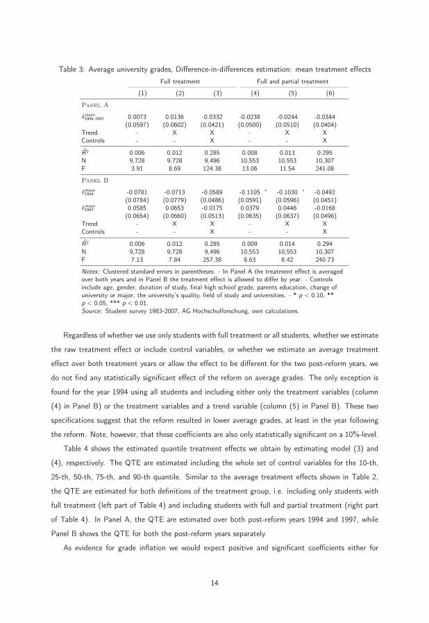
Table 3: Average university grades, Difference-in-differences estimation: mean treatment effectsFull treatment Full and partial treatment
(1) (2) (3) (4) (5) (6)
Panel A
δmean1994,1997 0.0073 0.0136 -0.0332 -0.0238 -0.0244 -0.0344
(0.0597) (0.0602) (0.0421) (0.0500) (0.0510) (0.0404)Trend - X X - X XControls - - X - - X
R̄2 0.006 0.012 0.285 0.008 0.013 0.295N 9,728 9,728 9,496 10,553 10,553 10,307F 3.91 8.69 124.38 13.06 11.54 241.08
Panel B
δmean1994 -0.0781 -0.0713 -0.0589 -0.1105 ∗ -0.1030 ∗ -0.0492
(0.0784) (0.0779) (0.0486) (0.0591) (0.0596) (0.0451)δmean1997 0.0585 0.0653 -0.0175 0.0379 0.0446 -0.0168
(0.0654) (0.0660) (0.0513) (0.0635) (0.0637) (0.0496)Trend - X X - X XControls - - X - - X
R̄2 0.006 0.012 0.285 0.009 0.014 0.294N 9,728 9,728 9,496 10,553 10,553 10,307F 7.13 7.84 257.38 8.63 8.42 240.73
Notes: Clustered standard errors in parentheses. - In Panel A the treatment effect is averagedover both years and in Panel B the treatment effect is allowed to differ by year. - Controlsinclude age, gender, duration of study, final high school grade, parents education, change ofuniversity or major, the university’s quality, field of study and universities. - * p < 0.10, **p < 0.05, *** p < 0.01.Source: Student survey 1983-2007, AG Hochschulforschung, own calculations.
Regardless of whether we use only students with full treatment or all students, whether we estimate
the raw treatment effect or include control variables, or whether we estimate an average treatment
effect over both treatment years or allow the effect to be different for the two post-reform years, we
do not find any statistically significant effect of the reform on average grades. The only exception is
found for the year 1994 using all students and including either only the treatment variables (column
(4) in Panel B) or the treatment variables and a trend variable (column (5) in Panel B). These two
specifications suggest that the reform resulted in lower average grades, at least in the year following
the reform. Note, however, that these coefficients are also only statistically significant on a 10%-level.
Table 4 shows the estimated quantile treatment effects we obtain by estimating model (3) and
(4), respectively. The QTE are estimated including the whole set of control variables for the 10-th,
25-th, 50-th, 75-th, and 90-th quantile. Similar to the average treatment effects shown in Table 2,
the QTE are estimated for both definitions of the treatment group, i.e. including only students with
full treatment (left part of Table 4) and including students with full and partial treatment (right part
of Table 4). In Panel A, the QTE are estimated over both post-reform years 1994 and 1997, while
Panel B shows the QTE for both the post-reform years separately.
As evidence for grade inflation we would expect positive and significant coefficients either for
14

Table 4: Average university grades, Difference-in-differences estimation: Conditional quantile treat-ment effects
Full treatment (N= 9,496) Full and partial treatment (N=10,307)
τ10 τ25 τ50 τ75 τ90 τ10 τ25 τ50 τ75 τ90
Panel A
δτ -0.0454 -0.0254 -0.0264 -0.0088 -0.0224 -0.0752 -0.0251 -0.0221 -0.0221 -0.0398(0.0562) (0.0399) (0.0414) (0.0423) (0.0532) (0.0532) (0.0399) (0.0386) (0.0379) (0.0477)
Panel B
δτ1994 -0.0878 -0.0516 -0.0712 -0.0708 -0.0458 -0.1018 -0.0312 -0.0381 -0.0735 -0.0542(0.0848) (0.0637) (0.0667) (0.0656) (0.0845) (0.0771) (0.0575) (0.0549) (0.0493) (0.0663)
δτ1997 -0.0033 0.0009 -0.0059 0.0066 -0.0165 -0.0069 0.0024 -0.0044 0.0061 -0.0300(0.0687) (0.0511) (0.0534) (0.0527) (0.0672) (0.0644) (0.0495) (0.0483) (0.0446) (0.0602)
Notes: Robust standard errors in parentheses. - In Panel A the treatment effect is averaged over both yearsand in Panel B the treatment effect is allowed to differ by year. - All regressions include as control variables atrend, age, gender, duration of study, final high school grade, parents’ education, change of university ormajor, the university’s quality, field of study and universities. - * p < 0.10, ** p < 0.05, *** p < 0.01.Source: Student survey 1983-2007, AG Hochschulforschung, own calculations.
all quantiles or at lower quantiles only. While the former supports evidence for a shift of the grade
distribution and a grade compression at better grades, the latter induces grade compression at the
lower end of the grade distribution. However, we do not find any evidence of grade inflation caused
by the introduction of the indicator-based funding reform.
We perform several robustness checks. Firstly, the multiple points in time before the introduction
of the reform that we observe in the data can be used to test whether the universities in North-
Rhine Westphalia anticipated the reform, i.e. whether our estimates suffer from an Ashenfelter’s
dip-problem, by including dummy variables for the years 1992 and 1989 in the regression. The results
do not give an indication that the universities changed their grading policy in anticipation of the
reform. Secondly, we estimate the treatment effect including only one of the control states, i.e. either
Baden-Wuerttemberg or Bavaria. Again, the results are not affected by this change.
5 Conclusion
The performance of a higher education system depends on both the sufficient supply of financial
resources and the efficient use of these resources. Starting in the early 1990s, several reforms were
implemented in the German higher education system to increase the universities’ efficiency and perfor-
mance. The German federal states, who are responsible for the organization of the higher education
system, followed a different pace in implementing these reforms, whose goal was the introduction
of managerial instruments in publicly funded institutions (New Public Management). In this paper,
we focus on the instrument of performance-based funding as it was an important part of these re-
forms. In contrast to the traditional funding system in which the budget of a given year was based
on past budgets and the outcome a university should produce, the new funding system takes the
15
actual performance of a university into account. The university’s performance is measured by a set
of indicators, e.g. the number of graduates or the amount of third party funds. Additionally, the
university’s performance is compared to the performance of other universities.
However, such a funding system is only able to increase university quality if they provide the
right incentives. Existing evidence shows that a funding system that concentrates on a few output
indicators may lead to wrong incentives. Using for example the number of graduates as an indicator
to determine the amount of public funds a university receives, the university may reduce quality
standards to increase the amount of graduates rather than increasing teaching quality. In such a case,
the reform may lead to grade inflation while the goal of increasing teaching quality is not reached.
In this paper we analyze whether the new funding system indeed caused wrong incentives to
German universities. In particular, we assess the influence of the indicator-based funding system on
the students’ average grades to identify whether the funding reform led to grade inflation. The case
of Germany, with the federal states being responsible for higher education, provides the possibility to
apply a difference-in-differences approach. However, due to data restrictions only short time effects can
be investigated. We choose North-Rhine Westphalia as the treatment state and Baden-Wuerttemberg
and Bavaria as the control states that we are able to observe for the years 1984 to 1997.
Since in NRW the indicator-based funding scheme was introduced in 1993, we observe two post
reform points in time, i.e. the years 1994 and 1997. The amount of states’ higher education funds
that was allocated based on indicators, however, was small. At the beginning of the reform, 0.1%
and later on 3% of public funds were allocated based on universities’ performance. The allocation
model incorporated several indicators that changed over the years. The two indicators that may lead
to grade inflation, i.e. the number of students and the number of graduates, account for 55% to
100% of the performance based allocated funds.
Evaluating the funding reform at the mean of average grades in a first step, we do not find
evidence for grade inflation. In a second step, we consider the entire grade distribution to evaluate
the effects of the reform by estimating quantile treatment effects. If grades are inflated, the grade
distribution either is shifted towards better grades and becomes compressed at the upper tail or it
becomes compressed at the lower end of the grade distribution. In the former case, all students get
better grades. For students with the best grades, the grades cannot become better resulting in a
compression at the upper tail of the distribution. In the latter case, the achievement requirements for
passing an exam are decreased and the distribution becomes compressed at the lower tail. Estimating
quantile treatment effects, we do not find evidence for grade inflation either.
Our results can be interpreted in two ways. On the one hand, the share of funds that is allocated
based on indicators may be too small to provide an incentive to the universities to inflate grades.
However, this in turn raises the question whether this low amount of indicator-based funding is able
to achieve improvements in the universities’ efficiency and performance. On the other hand, our
16

results may suggest that the universities did not inflate grades to get more funds. It should be also
stressed, that we are only able to estimate short term effects of the reform. It might well be the case,
that this short time period is not sufficient for the reforms to reach their full impact.
References
Anglin, P., and R. Meng (2000): “Evidence on grades and grade inflation on Ontario’s universi-
ties,” Canadian Public Policy, 36(3), 361–368.
Atkinson, A., S. Burgess, B. Croxson, P. Gregg, C. Propper, H. Slater, and D. Wil-
son (2009): “Evaluating the impact of performance-related pay for teachers in England,” Labour
Economics, 16(3), 251–261.
Bagues, M., M. S. Labini, and N. Zinovyeva (2008): “Differential Grading Standards and
University Funding: Evidence from Italy,” CESifo Economic Studies, 54(2), 149–176.
Bar, T., V. Kadiyali, and A. Zussman (2009): “Grade Information and Grade Inflation: The
Cornell Experiment,” Journal of Economic Perspectives, 22(3), 91–108.
Bauer, T. K., M. Fertig, and C. M. Schmidt (2009): Empirische Wirtschaftsforschung: Eine
Einführung. Springer, Berlin.
Burgess, S., C. Propper, H. Slater, and D. Wilson (2005): “Who wins and who loses
from school accountability? The distribution of educational gain in English secondary schools,”
The Centre for Market and Public Organisation 05/128, Department of Economics, University of
Bristol, UK.
Dickson, V. A. (1984): “An Economic Model of Faculty Grading Practices,” The Journal of
Economic Education, 15(3), 197–203.
Eaton, B. C., and M. Eswaran (2008): “Differential Grading Standards and Student Incentives,”
Canadian Public Policy, 34(2), 215–236.
Freeman, D. G. (1999): “Grade divergence as a market outcome,” The Journal of Economic
Education, 30(44), 344–351.
Froelich, M., and B. Melly (2010): “Estimation of quantile treatment effects with Stata,” Stata
Journal, 10(3), 423–457(35).
Jacob, B. A. (2005): “Accountability, incentives and behavior: the impact of high-stakes testing in
the Chicago Public Schools,” Journal of Public Economics, 89(5-6), 761–796.
17

Jacob, B. A., and S. D. Levitt (2003a): “Catching Cheating Teachers: The Results of an
Unusual Experiment in Implementing Theory,” Brookings-Wharton Papers on Urban Affairs, pp.
185–209.
(2003b): “Rotten Apples: An Investigation of the Prevalence and Predictors of Teacher
Cheating,” Quarterly Journal of Economics, 118(3), 843–877.
Joumady, O., and C. Ris (2005): “Performance in European higher education: A non-parametric
production frontier approach,” Education Economics, 13(2), 189–205.
Kingdon, G. G., and F. Teal (2007): “Does performance related pay for teachers improve student
performance? Some evidence from India,” Economics of Education Review, 26(4), 473–486.
Kocher, M. G., M. Luptacik, and M. Sutter (2006): “Measuring productivity of research in
economics: A cross-country study using DEA,” Socio-Economic Planning Sciences, 40(4), 314–332.
Koenker, R., and G. Bassett (1978): “Regression Quantiles,” Econometrica, 46(1), 33–50.
Krautmann, A. C., and W. Sander (1999): “Grades and student evaluations of teachers,”
Economics of Education Review, 18(1), 59–63.
Lavy, V. (2009): “Performance pay and teachers’ effort, productivity and grading ethics,” American
Economic Review, 99(5), 1979–2011.
Lechner, M. (2010): “The Estimation of Causal Effects by Difference-in-Difference Methods,”
University of St. Gallen Department of Economics working paper series 2010-28, Department of
Economics, University of St. Gallen.
Love, D. A., and M. J. Kotchen (2010): “Grades, Course Evaluations, and Academic Incentives,”
Eastern Economic Journal, 36, 151–163.
Martins, P. (2010): “Individual Teacher Incentives, Student Achievement and Grade Inflation,”
CEE Discussion Papers 0112, Centre for the Economics of Education, LSE.
Ministerium für Wissenschaft und Forschung des Landes Nordrhein-Westfalen
(n.d.): “Finanzautonomie, Kostenrechnung und erfolgsorientierte Mittelverteilung,” Schriftenreihe
zur Hochschulreform.
Nelson, J., and K. Lynch (1984): “Grade inflation, real income, simultaneity, and teaching
evaluation,” The Journal of Economic Education, 15(1), 21–37.
OECD (2010): Education at a glance - OECD indicators. OECD, Paris.
18

Reback, R. (2008): “Teaching to the rating: School accountability and the distribution of student
achievement,” Journal of Public Economics, 92(5-6), 1394–1415.
Sabot, R., and J. Wakeman-Linn (1991): “Grade inflation and course choice,” The Journal of
Economic Perspectives, 5(1), 159–170.
Schwager, R. (2008): “Grade Inflation, Social Background, and Labour Market Matching,” Dis-
cussion Paper No. 08-070.
Siegfried, J., and R. Fels (1979): “Research on teaching college economics: a survey,” Journal
of Economic Literature, 17(3), 923–969.
Simeaner, H., S. Dippelhofer, H. Bargel, M. Ramm, and T. Bargel (2007): “Datenal-
manach Studierendensurvey 1983 - 2007. Studiensituation und Studierende an Universitäten und
Fachhochschulen,” (Heft 51) Konstanz, Arbeitsgruppe Hochschulforschung, Universität Konstanz.
Statistisches Bundesamt (2004): Finanzen der Hochschulen 2002, Fachserie 11/ Reihe 4.5.
Statistisches Bundesamt, Wiesbaden.
Warning, S., and P. Welzel (2005): “A Note on grade inflation and university competition,”
Internet: http://www.fep.up.pt/conferences/earie2005/cd_rom/Session%20III/III.L/warning.pdf.
19

Appendix
Table A1: Number of observations by pre- and post-reform period, federal state, and year1984 1985 1986 1987 1988 1989 1990 1991 1992 1993 1994 1995
Baden-Wuerttemberg 1,036 (2) - 945 (2) - - 806 (2) - - 566 (2) - 499 (2) -Bavaria 1,414 (3) - 1,220 (3) - - 1,018 (3) - - 661 (3) - 552 (3) -Berlin 445 (1) - 423 (1) - - 334 (1) - - 286 (1) - 251 (1) -Brandenburg - - - - - - - - 96 (1) - 111 (1) -Hamburg 1,150 (2) - 1,002 (2) - - 829 (2) - - 696 (2) - 635 (2) -Hesse 773 (2) - 675 (2) - - 650 (2) - - 511 (2) - 427 (2) -Mecklenburg-West Pomerania - - - - - - - - 258 (2) - 143 (2) -North Rhine-Westphalia 1,076 (2) - 990 (2) - - 938 (2) - - 820 (2) - 635 (2) -Rhineland-Palatinate 134 (1) - 142 (1) - - 107 (1) - - 99 (1) - 84 (1) -Saxony - - - - - - - - 357 (2) - 387 (2) -Saxony-Anhalt - - - - - - - - 216 (2) - 121 (2) -Schleswig-Holstein 121 (1) - 98 (1) - - 103 (1) - - 82 (1) - 76 (1) -Thuringia - - - - - - - - 79 (1) - 63 (1) -
1996 1997 1998 1999 2000 2001 2002 2003 2004 2005 2006
Baden-Wuerttemberg - 466 (2) - - 481 (2) - - 606 (2) - - 443 (2)Bavaria - 538 (3) - - 687 (3) - - 980 (4) - - 515 (3)Berlin - 173 (1) - - 219 (1) - - 224 (1) - - 166 (1)Brandenburg - 146 (1) - - 195 (1) - - 190 (1) - - 127 (1)Hamburg - 505 (2) - - 506 (2) - - 569 (2) - - 458 (2)Hesse - 368 (2) - - 318 (2) - - 611 (3) - - 638 (3)Mecklenburg-West Pomerania - 204 (2) - - 315 (2) - - 256 (2) - - 255 (2)North Rhine-Westphalia - 491 (2) - - 507 (2) - - 543 (2) - - 416 (2)Rhineland-Palatinate - 52 (1) - - 69 (1) - - 226 (2) - - 179 (2)Saxony - 514 (2) - - 604 (2) - - 605 (2) - - 527 (2)Saxony-Anhalt - 126 (2) - - 224 (2) - - 221 (2) - - 201 (2)Schleswig-Holstein - 60 (1) - - 68 (1) - - 232 (2) - - 178 (2)Thuringia - 78 (1) - - 92 (1) - - 105 (1) - - 75 (1)
Note: The federal states of Bremen, Lower Saxony, and Saarland are not included in the sample. - The lighter graycells indicate the pre-reform and the darker gray cells the post-reform period. - Number of universities in parentheses.Source: Student survey 1983-2007, AG Hochschulforschung, own calculations.
20
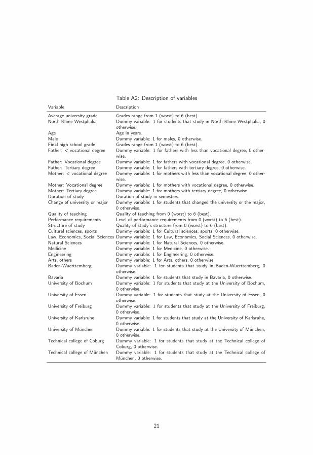
Table A2: Description of variablesVariable Description
Average university grade Grades range from 1 (worst) to 6 (best).North Rhine-Westphalia Dummy variable: 1 for students that study in North-Rhine Westphalia, 0
otherwise.Age Age in years.Male Dummy variable: 1 for males, 0 otherwise.Final high school grade Grades range from 1 (worst) to 6 (best).Father: < vocational degree Dummy variable: 1 for fathers with less than vocational degree, 0 other-
wise.Father: Vocational degree Dummy variable: 1 for fathers with vocational degree, 0 otherwise.Father: Tertiary degree Dummy variable: 1 for fathers with tertiary degree, 0 otherwise.Mother: < vocational degree Dummy variable: 1 for mothers with less than vocational degree, 0 other-
wise.Mother: Vocational degree Dummy variable: 1 for mothers with vocational degree, 0 otherwise.Mother: Tertiary degree Dummy variable: 1 for mothers with tertiary degree, 0 otherwise.Duration of study Duration of study in semesters.Change of university or major Dummy variable: 1 for students that changed the university or the major,
0 otherwise.Quality of teaching Quality of teaching from 0 (worst) to 6 (best).Performance requirements Level of performance requirements from 0 (worst) to 6 (best).Structure of study Quality of study’s structure from 0 (worst) to 6 (best).Cultural sciences, sports Dummy variable: 1 for Cultural sciences, sports, 0 otherwise.Law, Economics, Social Sciences Dummy variable: 1 for Law, Economics, Social Sciences, 0 otherwise.Natural Sciences Dummy variable: 1 for Natural Sciences, 0 otherwise.Medicine Dummy variable: 1 for Medicine, 0 otherwise.Engineering Dummy variable: 1 for Engineering, 0 otherwise.Arts, others Dummy variable: 1 for Arts, others, 0 otherwise.Baden-Wuerttemberg Dummy variable: 1 for students that study in Baden-Wuerttemberg, 0
otherwise.Bavaria Dummy variable: 1 for students that study in Bavaria, 0 otherwise.University of Bochum Dummy variable: 1 for students that study at the University of Bochum,
0 otherwise.University of Essen Dummy variable: 1 for students that study at the University of Essen, 0
otherwise.University of Freiburg Dummy variable: 1 for students that study at the University of Freiburg,
0 otherwise.University of Karlsruhe Dummy variable: 1 for students that study at the University of Karlsruhe,
0 otherwise.University of München Dummy variable: 1 for students that study at the University of München,
0 otherwise.Technical college of Coburg Dummy variable: 1 for students that study at the Technical college of
Coburg, 0 otherwise.Technical college of München Dummy variable: 1 for students that study at the Technical college of
München, 0 otherwise.
21
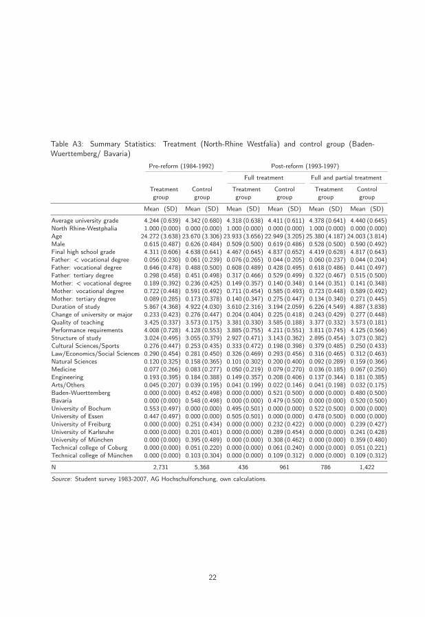
Table A3: Summary Statistics: Treatment (North-Rhine Westfalia) and control group (Baden-Wuerttemberg/ Bavaria)
Pre-reform (1984-1992) Post-reform (1993-1997)
Full treatment Full and partial treatment
Treatmentgroup
Controlgroup
Treatmentgroup
Controlgroup
Treatmentgroup
Controlgroup
Mean (SD) Mean (SD) Mean (SD) Mean (SD) Mean (SD) Mean (SD)
Average university grade 4.244 (0.639) 4.342 (0.680) 4.318 (0.638) 4.411 (0.611) 4.378 (0.641) 4.440 (0.645)North Rhine-Westphalia 1.000 (0.000) 0.000 (0.000) 1.000 (0.000) 0.000 (0.000) 1.000 (0.000) 0.000 (0.000)Age 24.272 (3.638) 23.670 (3.306) 23.933 (3.656) 22.949 (3.205) 25.380 (4.187) 24.003 (3.814)Male 0.615 (0.487) 0.626 (0.484) 0.509 (0.500) 0.619 (0.486) 0.528 (0.500) 0.590 (0.492)Final high school grade 4.311 (0.606) 4.638 (0.641) 4.467 (0.645) 4.837 (0.652) 4.419 (0.628) 4.817 (0.643)Father: < vocational degree 0.056 (0.230) 0.061 (0.239) 0.076 (0.265) 0.044 (0.205) 0.060 (0.237) 0.044 (0.204)Father: vocational degree 0.646 (0.478) 0.488 (0.500) 0.608 (0.489) 0.428 (0.495) 0.618 (0.486) 0.441 (0.497)Father: tertiary degree 0.298 (0.458) 0.451 (0.498) 0.317 (0.466) 0.529 (0.499) 0.322 (0.467) 0.515 (0.500)Mother: < vocational degree 0.189 (0.392) 0.236 (0.425) 0.149 (0.357) 0.140 (0.348) 0.144 (0.351) 0.141 (0.348)Mother: vocational degree 0.722 (0.448) 0.591 (0.492) 0.711 (0.454) 0.585 (0.493) 0.723 (0.448) 0.589 (0.492)Mother: tertiary degree 0.089 (0.285) 0.173 (0.378) 0.140 (0.347) 0.275 (0.447) 0.134 (0.340) 0.271 (0.445)Duration of study 5.867 (4.368) 4.922 (4.030) 3.610 (2.316) 3.194 (2.059) 6.226 (4.549) 4.887 (3.838)Change of university or major 0.233 (0.423) 0.276 (0.447) 0.204 (0.404) 0.225 (0.418) 0.243 (0.429) 0.277 (0.448)Quality of teaching 3.425 (0.337) 3.573 (0.175) 3.381 (0.330) 3.585 (0.188) 3.377 (0.332) 3.573 (0.181)Performance requirements 4.008 (0.728) 4.128 (0.553) 3.885 (0.755) 4.211 (0.551) 3.811 (0.745) 4.125 (0.566)Structure of study 3.024 (0.495) 3.055 (0.379) 2.927 (0.471) 3.143 (0.362) 2.895 (0.454) 3.073 (0.382)Cultural Sciences/Sports 0.276 (0.447) 0.253 (0.435) 0.333 (0.472) 0.198 (0.398) 0.379 (0.485) 0.250 (0.433)Law/Economics/Social Sciences 0.290 (0.454) 0.281 (0.450) 0.326 (0.469) 0.293 (0.456) 0.316 (0.465) 0.312 (0.463)Natural Sciences 0.120 (0.325) 0.158 (0.365) 0.101 (0.302) 0.200 (0.400) 0.092 (0.289) 0.159 (0.366)Medicine 0.077 (0.266) 0.083 (0.277) 0.050 (0.219) 0.079 (0.270) 0.036 (0.185) 0.067 (0.250)Engineering 0.193 (0.395) 0.184 (0.388) 0.149 (0.357) 0.208 (0.406) 0.137 (0.344) 0.181 (0.385)Arts/Others 0.045 (0.207) 0.039 (0.195) 0.041 (0.199) 0.022 (0.146) 0.041 (0.198) 0.032 (0.175)Baden-Wuerttemberg 0.000 (0.000) 0.452 (0.498) 0.000 (0.000) 0.521 (0.500) 0.000 (0.000) 0.480 (0.500)Bavaria 0.000 (0.000) 0.548 (0.498) 0.000 (0.000) 0.479 (0.500) 0.000 (0.000) 0.520 (0.500)University of Bochum 0.553 (0.497) 0.000 (0.000) 0.495 (0.501) 0.000 (0.000) 0.522 (0.500) 0.000 (0.000)University of Essen 0.447 (0.497) 0.000 (0.000) 0.505 (0.501) 0.000 (0.000) 0.478 (0.500) 0.000 (0.000)University of Freiburg 0.000 (0.000) 0.251 (0.434) 0.000 (0.000) 0.232 (0.422) 0.000 (0.000) 0.239 (0.427)University of Karlsruhe 0.000 (0.000) 0.201 (0.401) 0.000 (0.000) 0.289 (0.454) 0.000 (0.000) 0.241 (0.428)University of München 0.000 (0.000) 0.395 (0.489) 0.000 (0.000) 0.308 (0.462) 0.000 (0.000) 0.359 (0.480)Technical college of Coburg 0.000 (0.000) 0.051 (0.220) 0.000 (0.000) 0.061 (0.240) 0.000 (0.000) 0.051 (0.221)Technical college of München 0.000 (0.000) 0.103 (0.304) 0.000 (0.000) 0.109 (0.312) 0.000 (0.000) 0.109 (0.312)
N 2,731 5,368 436 961 786 1,422
Source: Student survey 1983-2007, AG Hochschulforschung, own calculations.
22

Table A4: Average university grades, Difference-in-differences estimation: mean treatment effectsFull treatment Full and partial treatment
(3) (3’) (6) (6’)
North Rhine-Westphalia -0.0774 ∗∗ (0.0357) -0.0772 ∗∗ (0.0357) -0.0747 ∗ (0.0374) -0.0750 ∗ (0.0373)Post-reform (1994,1997) -0.0374 (0.0339) -0.0212 (0.0297)Post-reform (1994) -0.0320 (0.0326) -0.0113 (0.0279)Post-reform (1997) -0.0402 (0.0415) -0.0436 (0.0440)δmean1994,1997 -0.0332 (0.0421) -0.0344 (0.0404)δmean1994 -0.0589 (0.0486) -0.0492 (0.0451)δmean1997 -0.0175 (0.0513) -0.0168 (0.0496)
Trend 0.0267 ∗∗∗ (0.0083) 0.0266 ∗∗∗ (0.0087) 0.0244 ∗∗∗ (0.0083) 0.0257 ∗∗∗ (0.0090)Age -0.0027 (0.0027) -0.0027 (0.0028) -0.0015 (0.0029) -0.0016 (0.0029)Male 0.0418 ∗∗ (0.0175) 0.0417 ∗∗ (0.0174) 0.0414 ∗∗ (0.0177) 0.0414 ∗∗ (0.0176)Final high school grade 0.2781 ∗∗∗ (0.0142) 0.2781 ∗∗∗ (0.0142) 0.2738 ∗∗∗ (0.0143) 0.2737 ∗∗∗ (0.0143)Father: vocational degree 0.0478 ∗∗ (0.0209) 0.0478 ∗∗ (0.0209) 0.0486 ∗∗∗ (0.0178) 0.0485 ∗∗∗ (0.0179)Father: tertiary degree 0.0839 ∗∗∗ (0.0223) 0.0840 ∗∗∗ (0.0223) 0.0831 ∗∗∗ (0.0200) 0.0830 ∗∗∗ (0.0201)Mother: vocational degree 0.0043 (0.0145) 0.0043 (0.0145) 0.0062 (0.0143) 0.0058 (0.0144)Mother: tertiary degree 0.0416 ∗∗ (0.0199) 0.0417 ∗∗ (0.0198) 0.0451 ∗∗ (0.0181) 0.0448 ∗∗ (0.0182)Duration of study 0.0055 (0.0051) 0.0054 (0.0051) 0.0056 (0.0050) 0.0056 (0.0050)Change of university or major 0.0275 (0.0175) 0.0276 (0.0176) 0.0274 ∗ (0.0163) 0.0275 ∗ (0.0163)Law/Economics/Social Sciences -0.1102 (0.0721) -0.1100 (0.0721) -0.1030 (0.0655) -0.1027 (0.0653)Natural Sciences -0.0425 (0.0579) -0.0426 (0.0579) -0.0312 (0.0544) -0.0312 (0.0543)Medicine 0.0859 (0.0938) 0.0862 (0.0937) 0.0964 (0.0883) 0.0975 (0.0882)Engineering -0.1258 ∗ (0.0688) -0.1258 ∗ (0.0687) -0.1196 ∗ (0.0641) -0.1196 ∗ (0.0640)Arts/Others 0.2037 ∗∗∗ (0.0545) 0.2037 ∗∗∗ (0.0545) 0.2082 ∗∗∗ (0.0513) 0.2082 ∗∗∗ (0.0513)Quality of teaching 0.2699 ∗∗ (0.1097) 0.2708 ∗∗ (0.1097) 0.2847 ∗∗∗ (0.1051) 0.2855 ∗∗∗ (0.1046)Performance requirements -0.5473 ∗∗∗ (0.0466) -0.5471 ∗∗∗ (0.0466) -0.5636 ∗∗∗ (0.0464) -0.5633 ∗∗∗ (0.0463)Structure of study 0.2772 ∗∗∗ (0.0805) 0.2767 ∗∗∗ (0.0804) 0.2734 ∗∗∗ (0.0804) 0.2725 ∗∗∗ (0.0803)University of Essen 0.0513 (0.0418) 0.0514 (0.0418) 0.0548 (0.0377) 0.0545 (0.0378)University of Karlsruhe -0.0848 ∗∗ (0.0379) -0.0850 ∗∗ (0.0378) -0.0814 ∗∗ (0.0368) -0.0813 ∗∗ (0.0369)University of München -0.0047 (0.0336) -0.0046 (0.0336) -0.0039 (0.0332) -0.0038 (0.0333)Technical college of München -0.1401 ∗∗∗ (0.0410) -0.1399 ∗∗∗ (0.0412) -0.1450 ∗∗∗ (0.0398) -0.1442 ∗∗∗ (0.0400)Constant 3.4489 ∗∗∗ (0.3273) 3.4465 ∗∗∗ (0.3271) 3.4617 ∗∗∗ (0.3159) 3.4600 ∗∗∗ (0.3152)
R̄2 0.285 0.285 0.295 0.294N 9,496 9,496 10,307 10,307F 124.38 257.38 241.08 240.73
Notes: Clustered standard errors in parentheses. - * p < 0.10, ** p < 0.05, *** p < 0.01.Source: Student survey 1983-2007, AG Hochschulforschung, own calculations.
23
Top Related