Languages
Pages
Legal


NASA/CR—20210000284
PEM Fuel Cell MODEL for Conceptual Design of Hydrogen eVTOL Aircraft Anubhav Datta Associate Professor Alfred Gessow Rotorcraft Center University of Maryland, College Park, Maryland
January 2021

NASA STI Program ... in Profile
Since its founding, NASA has been dedicated to the advancement of aeronautics and space science. The NASA scientific and technical information (STI) program plays a key part in helping NASA maintain this important role.
The NASA STI program operates under the auspices of the Agency Chief Information Officer. It collects, organizes, provides for archiving, and disseminates NASA’s STI. The NASA STI program provides access to the NTRS Registered and its public interface, the NASA Technical Reports Server, thus providing one of the largest collections of aeronautical and space science STI in the world. Results are published in both non-NASA channels and by NASA in the NASA STI Report Series, which includes the following report types:
• TECHNICAL PUBLICATION. Reports of completed research or a major significant phase of research that present the results of NASA Programs and include extensive data or theoretical analysis. Includes compilations of significant scientific and technical data and information deemed to be of continuing reference value. NASA counter-part of peer-reviewed formal professional papers but has less stringent limitations on manuscript length and extent of graphic presentations.
• TECHNICAL MEMORANDUM. Scientific and technical findings that are preliminary or of specialized interest, e.g., quick release reports, working papers, and bibliographies that contain minimal annotation. Does not contain extensive analysis.
• CONTRACTOR REPORT. Scientific and technical findings by NASA-sponsored contractors and grantees.
• CONFERENCE PUBLICATION. Collected papers from scientific and technical conferences, symposia, seminars, or other meetings sponsored or co-sponsored by NASA.
• SPECIAL PUBLICATION. Scientific, technical, or historical information from NASA programs, projects, and missions, often concerned with subjects having substantial public interest.
• TECHNICAL TRANSLATION. English-language translations of foreign scientific and technical material pertinent to NASA’s mission.
Specialized services also include organizing and publishing research results, distributing specialized research announcements and feeds, providing information desk and personal search support, and enabling data exchange services.
For more information about the NASA STI program, see the following:
• Access the NASA STI program home page at http://www.sti.nasa.gov
• E-mail your question to [email protected]
• Phone the NASA STI Information Desk at 757-864-9658
• Write to: NASA STI Information Desk Mail Stop 148 NASA Langley Research Center Hampton, VA 23681-2199

NASA/CR—20210000284
PEM Fuel Cell MODEL for Conceptual Design of Hydrogen eVTOL Aircraft Anubhav Datta Associate Professor Alfred Gessow Rotorcraft Center University of Maryland, College Park, Maryland
National Aeronautics and Space Administration Ames Research Center Moffett Field, CA 94035-1000
January 2021

This report is available in electronic form at
http://ntrs.nasa.gov

Contents
1 Abstract 3
2 Introduction 4
3 Hydrogen Infrastructure in the U.S. 14
4 Design Method 22
5 Analysis Method 26
6 Theory 276.1 Eh and Er . . . . . . . . . . . . . . . . . . . . . . . . . . . . . . . . . . . . . . . . . . . . . . . 276.2 The i − v Curve . . . . . . . . . . . . . . . . . . . . . . . . . . . . . . . . . . . . . . . . . . . 286.3 H2 flow . . . . . . . . . . . . . . . . . . . . . . . . . . . . . . . . . . . . . . . . . . . . . . . . 306.4 H2 Energy and Storage . . . . . . . . . . . . . . . . . . . . . . . . . . . . . . . . . . . . . . . . 336.5 Air flow . . . . . . . . . . . . . . . . . . . . . . . . . . . . . . . . . . . . . . . . . . . . . . . . 38
7 Balance of Plant 42
8 Weights 48
9 Software Overview 56
10 List of inputs and outputs 57
11 Example: Baseline 80 kW 72
12 Example: Modern 80 kW 77
13 Example: Modern 500 kW 88
14 Rotorcraft Sizing 9714.1 Basic Sizing . . . . . . . . . . . . . . . . . . . . . . . . . . . . . . . . . . . . . . . . . . . . . . 9714.2 Essential Refinements . . . . . . . . . . . . . . . . . . . . . . . . . . . . . . . . . . . . . . . . 10014.3 Example: NASA Electric Quad-rotor . . . . . . . . . . . . . . . . . . . . . . . . . . . . . . . . 10814.4 Example: Maryland Electric Quad-rotor . . . . . . . . . . . . . . . . . . . . . . . . . . . . . . 11314.5 Example: Single Main-Rotor and Tail-rotor . . . . . . . . . . . . . . . . . . . . . . . . . . . . 119
15 Summary and Conclusions 124
16 Technology Drivers, Requirements and Recommendations 127
17 References 132
18 Source Code and Input Decks 135
2

1 Abstract
A model and software for design and analysis of a Proton Exchange Membrane fuel cell (PEMFC) systemare developed for hydrogen eVTOL aircraft. Examples are provided of stacks designed for 80 kWe and 500kWe net electrical power. Examples are provided of eVTOL designed for 250 and 400 lb payload. Thetrade-offs included stack characteristics, hydrogen storage characteristics, and aircraft payload and range.The objectives were to identify the key technology drivers of a hydrogen rotorcraft, establish technologytargets for a viable aircraft, and recommend research to address the fundamental pre-competitive barriers.The current U.S. infrastructure on hydrogen informed the targets and recommendations. The key conclusionis that the advances made in cell electrochemical power density over the last decade might allow a PEMFCsystem to meet, or even beat, piston engine powered light-utility rotorcraft. The development must focuson the key drivers of a hydrogen eVTOL. The drivers are ultra-light stack cooling and short-term hydrogenstorage. A stack system of net electrical power 100−150 kWe with specific power 1.1 kWe/kg including air,cooling, and electrical subsystems, and a tank storage of 15% weight fraction hydrogen are the minimumtargets to meet the performance of a modern piston-engine rotorcraft, with a range of 180 nautical miles,payload of 400 lb, and gross weight of about 1400 lb. This is defined as the objective aircraft. If only onetarget is met, an aircraft of half the range could be produced, with a 30% greater gross take-off weight.This is defined as an intermediate aircraft. Because definitive conclusions are premature without weightsand loads data on a flight-worthy stack system, it is recommended that a fuel cell powered hydrogen eVTOLdemonstrator be built and flown. The existing hydrogen infrastructure for cars provide ample opportunity tocreate a pilot program. About 12 metric tons of retail hydrogen are available for cars every day in California,which is less than 0.05% of the yearly hydrogen production in the U.S.. A hypothetical fleet of 100 aircraft,operating 3 flights a day, would increase the demand by 2.25 tons per day and require 140 MWh of renewableelectricity for green hydrogen.
3

2 Introduction
This report describes a model and software for design and analysis of a Proton Exchange Membrane (alsoknown as Polymer Electrolyte Membrane) fuel cell (PEM FC) system. The software sizes a PEMFC systemto meet certain specified requirements (design) and then predicts its performance for a set of conditions(analysis). The software is meant to support the conceptual design and technology assessment of a PEMFCpowered hydrogen electric-Vertical Take off and Landing aircraft.
An electric-Vertical Take off and Landing aircraft (eVTOL) is defined as a vertical lift aircraft propelledby electric power and capable of carrying people. A hydrogen eVTOL (H2eVTOL) derives its electrical powerfrom a hydrogen PEMFC. The abbreviation VTOL is used synonymously with rotorcraft. The notationsH2, H and h2 are used as shorthands for hydrogen. The words fuel cell, PEM FC, and PEMFC are usedinterchangeably.
A PEMFC system consists of a fuel stack, ancillary subsystems, and hydrogen storage. The softwarefacilitates the description and analysis of a typical general-purpose PEMFC system, while retaining theability to assess new and advanced concepts. The software implements low-fidelity phenomenological modelsbased on test data and look-up tables. For ancillary subsystems, device level models are used which can becalibrated to test data.
The models were developed for eVTOL sizing and analysis reported in Datta and Johnson 2012 and2014, Ng and Datta 2019, and Ng, Patil and Datta 2021. They are consolidated here. The models for stackweight and cooling system are expanded. Cell characteristics are updated with recent advances reported bythe U.S. Department of Energy Hydrogen Program (DOE HP).
A section on rotorcraft sizing is included, with examples to illustrate how the fuel cell models enterand affect sizing. The rotorcraft sizing model is kept simple so it can be reproduced easily and mightserve as a common-basis for technology assessment by fuel cell, hydrogen, and rotorcraft specialists. Theexamples are chosen so that operations are feasible within the current U.S. hydrogen infrastructure. Thesizing methodology is generic however, and can be easily extended to larger aircraft.
Datta and Johnson 2012, 2014 made assessments of battery and hydrogen eVTOL using DOE HP tech-nology of the 2000s and gave a set of technology targets for practical eVTOL. The fuel cell targets have nowbeen met by the DOE HP. The advances have been scaled up to 80 kW power, tested, peer-reviewed, andpublished, see Ahluwalia, Wang and Steinbach 2016 and Thompson et al 2018. The reported cell character-istics have nearly reached the pure-oxygen limit. The objective of this report is to assess the implications ofthese advances on a conceptual hydrogen eVTOL, identify the key technology drivers for a viable aircraft,and establish clear technology targets for the future.
Unique opportunities of growth in PEMFC and hydrogen infrastructure may be afforded by eVTOL.The usual reservations about PEMFC, such as the lack of regenerative braking and heavy hydrogen storage,do not apply to eVTOL. First, there is no regenerative braking in VTOL, so batteries provide no specialadvantage. Second, very short duration on-board storage is needed (1-3 hrs), so lighter tanks are conceivable.The problem of low pressures at high altitudes, encountered in an airliner, is also bypassed; rotorcraft areby design low altitude aircraft. The requirement for quiet flight in urban / civil missions eliminates thehydrogen combustion engine as an option. Combustion also produces NOx, a criteria air pollutant. ThusPEMFC is the natural choice for clean and quiet hydrogen eVTOL.
4

Background
There is a vast literature on fuel cells. Modern texts such as Barbir 2005, Spiegel 2007, O’Hayre, Cha,Colella and Prinz 2009 and Dicks and Rand 2018, cover them comprehensively. Many peer-reviewed journalspublish fuel cell research (Table 1), including Fuel Cells from Fundamentals to Systems (Wiley) and Int.
J. of Hydrogen Energy (Elsevier), that are dedicated exclusively to the topic. The papers mainly reportadvances in material science and electrochemistry. Some that are relevant to aeronautics are also publishedin various AIAA journals, but they are few. Only a single paper appears in the Journal of the American
Helicopter Society. Fuel cells are not mature yet to be a viable means of aircraft propulsion.
Advanced Materials Fuel Cells from Fundamentals to SystemsAdvanced Energy Materials Int J of Energy ResearchAngewandte Chemie (in German) Int J of Hydrogen EnergyComputers and Chemical Engineering J of Power SourcesChemical Engineering Science J of Electrochemical Society (ECS)Chemical Reviews J of Materials Chemistry (A, B, C)ChemSusChem J of Physical Chemistry (A, B, C)Electrochimica Acta J of Membrane ScienceEnergies Nature MaterialsEnergy and Fuels Nature EnergyEnergy and Environmental Science Renewable and Sustainable Energy ReviewsEnvironmental Science and Technology World Electric Vehicle Journal
Table 1: Some journals that publish fuel cell research.
Figure 1 highlights some of the interesting past and present applications of fuel cells in aerospace.There is a long history of fuel cells in space. The first fuel cell powered spacecraft was the Gemini
V launched in 1965. The PEMFC system was developed by General Electric beginning 1962. Its legacycontinues to this day; see Burke 2003 and Burke 2012 for reviews of hydrogen and fuel cell programs atNASA. Space fuel cells must use pure oxygen and are often needed in a regenerative (reverse) mode whereelectricity (from solar panels) is used to produce hydrogen and oxygen from water. The power requiredis usually low, around 1-10 kW, and the consideration of weight less important than in aviation. Reliableoperation over extreme duration (years and perhaps decades) is more crucial.
The modern PEMFC matured in ground and automobile sectors. These PEMFC extract oxygen from airand operate in the normal (or forward) mode to generate electricity while producing water from hydrogen andoxygen. The electricity drives a motor. The power output of automobile fuel cells is of the order of 100 kW.The U.S. Department of Energy began its Hydrogen Program in 2002, pursuant to the Hydrogen Future Actof 1996 and the Matsunaga Hydrogen RD&D Program Act of 1990. The legislative mandate of the HydrogenProgram covered industrial, residential, transportation, and utility applications. By transportation, onlyground vehicles were meant. The Founding Agreement — FreedomCAR in 2002, was a Fuel Partnershipbetween DOE and the U.S. Council of Automotive Research. Even though the Hydrogen Program citedaerospace experience in its mandate as context for accelerating wider application of hydrogen technologies,aviation always remained outside its scope. The Year-2020 DOE Hydrogen Program Plan (released 12November 2020) mentions aviation in passing as one of many Other emerging opportunities (pg. 29) andlists a program called REEACH (pg. 40) but otherwise places no emphasis on aviation. Thus, the progressachieved in the Hydrogen Program generally remains outside the purview of aviation experts. A few isolatedattempts from outside are made from time to time, such as a conversion study of Boeing 787 at Sandia Labs(Pratt et al 2011) or a conversion study of Robinson R22 at NASA Ames (Datta and Johnson 2014), butthey are limited to paper studies.
Inspired by space and ground applications, experimental airplanes have been flown with PEMFC. The
5

Figure 1: Fuel cells in aerospace. Space applications use pure oxygen fuel cells. Aircraft use air breathing fuel cells.
6

unmanned Global Observer prototype (15.24 m wing span, 1/3-scale) by AeroVironment is the earliest doc-umented fuel-cell powered aircraft that flew successfully (an earlier attempt by a similar aircraft designatedHP-03 ended in crash on its first flight on 26 June 2003; the crash was due to aeroelastic problems notthe fuel cells, see NASA-NOAA crash report by Noll et al 2004). The Global Observer used PEMFC withliquid hydrogen as fuel (the HP-03 was originally meant to produce hydrogen on board using a regenerativefuel cell, but the actual aircraft was built with a normal fuel cell to bypass problems encountered duringdesign of the regenerative system). The Global Observer prototype flew on 26 May 2005 at the U.S. Army’sYuma Proving Grounds in Arizona. Details remain unpublished. Since then, full-scale Global Observers(53 m wing span) have made many successful flights (the first prototype crashed 18 hrs into its 9th flight),but very little technical information is available in the public domain. A number of manned airplanes havealso been flight tested since then. These include the single-occupant/pilot Boeing (Spain) Fuel Cell airplane(Lapena-Rey et al 2010), the single-occupant/pilot DLR Antares (Kallo et al 2015) and the four-occupantDLR Hy4 (unpublished, but some information can be found in Flade et al 2016). Gaseous hydrogen was usedas fuel for both. The Boeing (Spain) and DLR programs are well documented, but weight information isunavailable. Only the Naval Research Laboratory Ion Tiger Program, which flew a small 0.55 kW unmannedairplane on 0.5 kg of liquid hydrogen, documented weights methodically (across several publications between2011-2014, see Stroman et al 2014 and Swider-Lyons et al 2014 for final numbers). Most of these efforts usederivatives of automobile fuel cells.
Inspired by airplanes, small experimental rotorcraft have been flown with PEMFC. A battery poweredsmall kit helicopter Maxi-Joker 2 was converted to a fuel cell helicopter (2 m single main rotor diameter,10 kg gross take-off weight, and 4 kg empty weight) by United Technologies Research Corporation (UTRC)(Moffitt and Zaffou 2012). It flew on 11 October 2009 at East Hartford Campus of UTRC. Some weightinformation is available. The power density of the stack was 0.65 kW/kg, stack including ancillaries was0.5 kW/kg, the stack weight was 3.4 kg, and the maximum power output was 1.75 kW. Gaseous hydrogenwas stored at 289 bar, in a 2.3% weight fraction tank. The PEMFC was custom made, the tank was acommercial unit. Since then, commercial rotary-wing drones have made their debut in the UAS market anddemonstrated extreme endurance compared to batteries. Little to no information on weight breakdown ispublished.
The weights that are available in public are plotted in Fig 2. Stack power is plotted versus weight. OnlyToyota, Honda, Ion Tiger, and the UTRC helicopter data are obtained from peer-reviewed sources. Mostsources provide only the stack weight. Some provide weights of ancillary subsystems but do not specify whatthey are. Whether the power reported is gross or net electrical is unspecified. The commercial rotary-wingdrones report total weight including hydrogen. Fewer details are available for the under-water systems. Outof this incomplete and often inconsistent information, no useful trends or sensible weight models can begenerated.
A number of previous NASA reports describe PEMFC weight models for special-purpose applications.These include, Burke 1999, on regenerative PEMFC performed in the context of AeroVironment’s high-altitude unmanned solar Centurion airplane (a precursor to the Helios series culminating in the HP-03),Colozza 2002, on hydrogen storage weights for aircraft applications, and Colozza and Jakupca 2019, onthermal sizing for ground-based systems on Mars.
The objective of this work is a general-purpose method with well-defined models for weights. Users withaccess to measured weights should be able to calibrate the models and make reliable assessment of moreadvanced concepts. The models are simple, as appropriate for a conceptual design environment, yet rootedin test data, geometry and materials. Only PEMFC is considered as it is the lightest of all fuel cells (highestspecific power, kW/kg) and at present the only path to clean, renewable, emissions-free flight. Only air-breathing PEMFC is considered, and only the normal or forward operation is modeled, as appropriate foreVTOL.
7

10-1 100 101 102 103
Stack Weight, kg
10-1
100
101
102
103
Pow
er, k
W
2.0 kW/kg
0.50
0.25 kW/kg1.0
UAV fixed-wingUAV rotary-wing
UTRC helicopter2009
Under-water vehiclescommercial motive
commercial stationary
Airplanes
Toyota 2008
Honda2005
Toyota 2015
DOE hyd prog2015 target
Honda 2009
Figure 2: State-of-the-art power and weight of PEMFC systems of < 500 kW.
8

Units and Standard Conventions
Throughout the report, SI units are used unless otherwise mentioned. Non-SI units are used for somecomponents where they are the norm to maintain uniformity in literature. The pertinent conversions aredescribed below.
Energy :
1 Watt-hr (Wh) = 3600 Joule (J)
1 kilo Watt-hr (kWh) = 3.6 Mega-Joule (MJ)
Pressure :
1 atm = 101, 325 Pascal (Pa) = 1.01325 bar = 14.6959 lbf/inch−2 (psi)
1 bar = 0.1 Mega-Pascal (MPa)
Temperature :
1 Celsius (C) = 1 Kelvin (K) − 273.15
Volume :
1 Liter (L) = 0.001 m3
1 U.S. gallon (gal) = 3.7854 L
1 cubic ft/min (CFM) = 14.72× 10⁻⁴ m3/s = 1.472 L/s
Throughout the report, ISA and STP-NIST standard conventions are used (Table 2). The STP-IUPACis also used in fuel cell literature. It is identical to STP-NIST except for a small difference in temperature.
Standard T T p p pK C Kelvin bar kPa atm
ISA/SL 15 288.15 1.01325 101.325 1STP-NIST 25 298.15 1 100 0.9869STP-IUPAC 0 273.15 1 100 0.9869
Table 2: Standard conditions.
The Proton Exchange Membrane Fuel Cell (PEMFC)
A Proton Exchange Membrane (also known as Polymer Electrolyte Membrane) fuel cell (PEMFC) is shownin Fig 3. The basic operation is as follows.
Hydrogen flows into the anode electrode and decomposes into protons and electrons.
H2 → 2H+ + 2e− Anode, release of electrons, oxidation
The electrons pass through an external circuit which is how current is generated. The protons pass throughan electrolyte membrane.
Air flows into the cathode electrode and the oxygen combines with protons and electrons to producewater (vapor or liquid).
1/2O2 + 2e− + 2H+ → H2O Cathode, capture of electrons, reduction
Nitrogen and other gases simply pass through without reaction.Overall, a fuel cell extracts energy released during the following reaction as charge with a voltage
H2 + 1/2 O2 → H2O
9

Figure 3: A proton exchange membrane fuel cell.
Hydrogen and air enter a fuel cell through channels built into what are called bipolar plates. The bipolarplates can also contain channels for coolant. The channels have intricate design. The bipolar plates are theheaviest parts of a fuel cell and can contribute up to 80% of its weight.
The anode and cathode electrode each consist of two parts: a gas diffusion layer (GDL) and a catalystlayer (Anode or Cathode catalyst layers (ACL or CCL)). The hydrogen and air diffuse through these layers.The GDL is typically made of carbon paper or cloth, carbon powder, and polytetrafluoroethylene (PTFE).Teflon is a brand name of PTFE made by Chemours, a spin-off of DuPont (DuPont discovered the compoundin 1938). The catalyst layer is typically made of Platinum on Carbon (Pt/C) powder and an ionomer. Nafion,a brand name for sulfonated tetrafluoroethylene, is a typical ionomer (also discovered by DuPont, in late1960s). In its simplest form, the electrode is just a carbon cloth coated with Pt/C on one side. The typicalcatalyst loading varies from 0.1 − 0.4 milligram of Pt/cm2. The catalyst is responsible for breaking downhydrogen into protons and electrons. Both the GDL and ACL/CCL are porous and partially hydratedstructures. The dispersed carbon particles have a typical diameter of 0.7 µm whereas the Pt nanoparticlesparched on top of carbon have typical diameters of 3 − 5 nm. Large pores in between the particles formducts for hydrogen and oxygen to diffuse from the bipolar plates to the respective catalyst layers. Thesmaller pores form ducts for water. Once split, hydrogen passes its electrons to Platinum and protons tothe electrolyte membrane. The membrane is also a polymer, typically Nafion. When sufficiently hydrated itis an excellent conductor of protons. The membrane and the electrodes together are called the MembraneElectrode Assembly (MEA).
The electrons flowing through the outer circuit is captured back into the cathode catalyst layer (CCL)by Platinum. At the cathode, oxygen diffuses through the GDL to react with the protons coming fromthe membrane and electrons from Platinum to produce water (vapor or liquid) and heat. So the cathodeside generates water and heat. Platinum ensures water, not hydrogen peroxide, a toxic gas, is produced.Platinum makes fuel cells expensive.
It is crucial that the membrane is sufficiently hydrated for proton conduction. Because water and heatare generated at the cathode, the membrane on the cathode side tends to saturate, while the membraneon the anode side tends to dehydrate. This reduces the conductivity of the protons. To limit this prob-lem, the cell is fed with humidified gases at temperatures higher than the cell temperature. However, toomuch humidification — meant for the membrane — can flood the electrodes and prevent gas transport to
10

the membrane/catalyst interface. Balanced humidification is critical — too little or too much are bothdetrimental.
Unlike a combustion engine, a fuel cell has no exhaust gases to carry heat out, so the heat must beremoved entirely by other means. The low temperature operation of the stack (65-85C) makes it harderfor coolants to carry heat out; the small temperature difference between stack and the ambient also requirea large radiator. Radiators are heavy, and a major overhead in high power stacks. Cooling can be a majorbarrier in aviation unless lighter weight methods are devised.
The PEMFC System
Cells connected in parallel form a PEMFC stack. Ancillary subsystems are needed to operate the stack. Thestack and the ancillary subsystems form the PEMFC stack system. The stack system, and the fuel tank andfuel delivery subsystem form the total PEMFC system.
The PEMFC system model is sketched in Fig 4. The architecture mimics a modern automobile PEMFCsystem. The subsystems are listed below.
1. Stack
2. Air management system
3. Low temperature cooling (LTC) system
4. High temperature cooling (HTC) system
5. Water management system
6. Electrical system
7. Hydrogen tank and delivery system.
The stack and the tank are the principal subsystems. Not all ancillary subsystems are needed to model everyPEMFC system.
The design method sizes the PEMFC system. The block diagram for sizing is shown in Fig 5 (top). Adesign power PD is specified and the stack is sized to generate this power. The net electrical power PDe
is the power generated minus the power to operate the ancillary subsystems which is called the balance ofplant PBOP .
PDe = PD − PBOP
The design method iterates the sizing method to compensate for the balance of plant and achieve a specifiednet electrical power. The block diagram for design is shown in Fig 5 (bottom).
The analysis method predicts the performance of a PEMFC system after it is designed under variousoff design conditions. The block diagram of analysis is shown in Fig 6. The current is specified and thevoltage and net electrical power are calculated. Only steady-state current is considered. Ng and Datta 2019measured the stack transients and found them fast (similar to a Li ion battery) and first order (resistive andcapacitive behavior). The system transients are therefore determined by air and cooling system transients.These are discipline dependent (car or aircraft) and in absence of data left out of scope.
Cost analysis is left out of scope. Cost analysis for fuel cell cars are published by the DOD HP, see forexample Thompson et al 2018 for a recent analysis for high-volume manufacturing scenarios. Cost analysisof fuel cell eVTOL may be premature before an airworthy stack system is built and tested and a clearunderstanding of parts and supply chain is acquired.
11

Figure 4: A PEMFC system. The subsystems shown are air, low temperature cooling (LTC), stack, high temperature cooling(HTC), and water (H20). The lines and arrows show the flow of air, coolant, and water. The electrical subsystem (not shown)covers transmission and distribution of power from the stack to the drive as well as controllers and power to each subsystem.P=pump. M=motor. T=turbine. C=compressor. Humid=humidifier.
12

Figure 5: Design block diagrams.
Figure 6: Analysis block diagram.
Outline of Report
In the sections that follow, the existing U.S. hydrogen infrastructure is described first. It sets the contextfor design. The design and analysis steps are outlined in Sections 4 and 5 respectively. The theory behindthe steps are described in Section 6. Sections 7 and 8 are dedicated respectively to power consumption andweight models. Section 9 outlines the software. Section 10 describes the inputs and outputs. Example fuelcell designs are described in Section 11 (Yr-2000 cell technology, 80 kWe stack), Section 12 (modern cells, 80kWe stacks) and Section 13 (modern cells, 500 kWe stacks). The 80 kWe models can be used for cars. The500 kWe models are meant for aviation. The examples are templates to be calibrated with test data whenthey become available. Section 14 describes a simplified rotorcraft sizing method which is used in exampleslater to illustrates how the fuel cell models enter and affect sizing. The method is kept deliberately simple soit can be reproduced by non-rotorcraft specialists. Three examples are given: 1) a single-occupant conceptualNASA electric quad-rotor, 2) a two-occupant conceptual Maryland electric quad-rotor, and 3) a two-occupantmain rotor-tail rotor helicopter calibrated loosely to a R22 Beta II weight, range, and payload. The thirdexample allows technology targets to be calibrated for a certified airframe. Section 15 gives summary andconclusions. Section 16 gives the technology drivers, and requirements and makes recommendations for ahydrogen eVTOL pilot program. The software is appended at the end.
13

3 Hydrogen Infrastructure in the U.S.
This section describes the hydrogen infrastructure in the U.S., from supply, to retail to codes and standards.Infrastructure informed design, particularly tank and aircraft size, and the scale of examples.In 2020, 9 million metric tons of hydrogen were produced in the U.S., and 87 million globally.Globally, hydrogen is produced from various sources (Table 3). They are color coded accordingly, although
there is no formal or universal convention. About 95% of hydrogen is produced from fossil fuels. Thishydrogen is coded grey or brown. The production process emits 9–12 tons of CO and CO2 per ton ofhydrogen from grey to brown. When backed by carbon capture and storage it is coded blue. The energycontent of hydrogen is 39 kWh/kg. The production efficiency is around 90% which means 43 kWh/kg ofenergy is spent to produce this hydrogen. About 4% of hydrogen is produced from water electrolysis. Whenthe electricity is derived from wind or solar, the hydrogen is coded green. When the electricity is from nuclear,it is coded purple. About 250 megawatts (MW) are presently dedicated to producing green hydrogen. Theproduction efficiency is around 70% which means 55 kWh/kg of energy is spent to produce green hydrogen.
% Produced Source Process Color
48% Natural gas 1. Steam reformation grey
If backed by carbon capture & storage blue
2. Methane pyrolysis with turquoise
no green house gas emissions
30% Petroleum Steam reformation grey
18% Coal Coal gasification or carbonisation brown
4% Renewable Water electrolysis with electricity green
Electricity from nuclear power purple
Table 3: Sources of hydrogen.
The price of grey-brown hydrogen is U.S. $1-3/kg. The price of green hydrogen varies widely. Often$5-19/kg is quoted but that number is the price of electricity. In the U.S., the average price of electricityis 13 cents/kWh, but variation across states, Hawaii-34, California-22, Maryland-13, to Washington-9.5cents/kWh, gives the range. Then there is the cost of transportation (except green hydrogen producedon-site) and compression or liquefaction.
Globally, hydrogen has a vast industrial usage (Table 4). Only a tiny fraction is used in transportation.A significant amount is used in oil refining. So even though hydrogen is produced largely from fossil fuels,fossil fuels are also produced using hydrogen.
% Use Industry
25% Oil refining through hydrodesulfurization and hydrocrackingHydrodesulfurization — removal of Sulfur from gasoline, jet fuel, kerosene etcHydrocracking — conversion of heavy fuel into diesel, jet fuel, kerosene etc
55% Ammonia production through Haber-BoschHaber-Bosch — artificial fixation of nitrogen with hydrogen
10% Methanol production10% Other, such as HCl production, hydrogenation, coolant, transportation
Table 4: Usage of hydrogen.
14

Hydrogen is transported through pipelines and trucks. According to the U.S. DOE Office of EnergyEfficiency and Renewable Energy, there are 1600 miles of hydrogen pipelines in the U.S.. They are ownedby merchant hydrogen producers, and located near large users such as oil refineries and ammonia plants,most of which are in the Gulf Coast region. Beyond pipelines, hydrogen is distributed through trucksthat haul trailers stacked with long pressure-tight steel cylinders of gaseous hydrogen (CGH2) called tubetrailers. The cylinders are limited to 250 bar pressure, per U.S. Department of Transportation regulation,and carry typically 380 − 420 kg of hydrogen. The capacity of the truck is limited by the weight of steelcylinders. Specially insulated, cryogenic (−253C), tanker trucks haul liquid hydrogen (LH2). Liquefactioncan consume up to 30% of hydrogen energy. In addition, some hydrogen can evaporate (boil-off), more so ifthe tank surface to volume ratio is high as in small trucks. Typical tanks can carry from 1,500–25,000 gallons(400–6,500 kg, using density of 70 kg/m3) of liquid hydrogen at 1 bar. Thus, liquid trucks are economicalfor longer distances and larger amounts of hydrogen, for rocket launches for example. Hydrogen is thendispensed into compressed gas cylinders at the retail stations or poured directly as liquid. Compared to the1600 miles of hydrogen pipeline, there are 3 million miles of natural gas pipelines, as of December 3, 2020,per U.S. Energy Information Administration. A study on how hydrogen might be blended into existingnatural gas pipelines can be found in the NREL report by Melaina, Antonia and Penev 2013.
The Alternative Fuels Data Center, under the Office of Energy Efficiency and Renewable Energy, U.S.DOE, maintains a data base on fleet, fuels and fueling stations in the U.S. and Canada. According to thisdatabase, as of June 2021, there are 68 open hydrogen stations in the U.S.; 19 are private and 49 are publicretail outlets. These provide fuel to the 10,665 fuel cell cars, sold and leased, and 48 fuel cell buses currentlyin operation. Almost all outlets provide compressed gas at 350 or 700 bar.
State Fueling station City Pressure
bar
Arizona Nel hydrogen-Nikola, 4141 E Broadway Rd Phoenix 350
California SunLine Transit Agency, 32-505 Harry Oliver Trail Thousand Palms 350
California Honda MC Formula Station, 1900 Harpers Way Torrance 700
California AC Transit, Oakland, 1100 Seminary Ave Oakland 350
California AC Transit, Emeryville, 1172 45th St Emeryville 350
California Orange County Trans Authority, 4301 MacAurthur Blvd Santa Ana 350
Colorado DOE/NREL, 15013 Denver West Pkwy Golden 350, 700
Connecticut Tri-Gen, 539 Technology Park Dr Torrington 350
Delaware Air Liquide, 200 Gbc Dr Newark unknown
Hawaii Blue Planet Research, 71-1645 Mamalahoa Hwy 2 Kailua-Kona 350
Massachusetts Bus Transit Auth., Charlestown Garage, 21 Arlington Ave Boston 350
Massachusetts Greentown Labs, 444 Somerville Ave Somerville 700
Michigan Ford Lab, Miller Rd and S Dix St Dearborn 350, 700
Michigan Bus Transportation Authority, 5051 S Dort Hwy Grand Blanc 350
New York Hempstead - Dept of Cons & Waterways, 1401 Lido Blvd Point Lookout 350
Ohio Regional Transit Auth., Stark Area, 1600 Gateway Blvd SE Canton 350
Ohio DOD/Defense Supply Center Columbus unknown
Virginia DOD/Fleet Service Center, 7847 Senate St, Bldg 126 Richmond unknown
Washington Army/Ft Lewis, McKinley Ave & Garfield St Ft Lewis unknown
Table 5: Private outlets of hydrogen in the U.S..
The 19 private outlets are listed in Table 5 along with their tank pressure capability. Of the 49 publicretail outlets, 48 are in California. The only other outlet is in Honolulu, Hawaii, a Toyota Mirai dealershipin 2850 Pukoloa St run by Servo. It produces 20 kg of hydrogen per day and allows up to 4 car fill-ups atpressures of 350 and 700 bar. The California Air Resources Board (CARB) maintains a yearly count of fleetand fueling stations in California (see CARB 2020). The count for Yr-2019 was reported as 43 by CARBon July 3, 2020. The projection for Yr-2020 at the time was 58. The unofficial count as of July 2021 by the
15

Figure 7: California public outlets of hydrogen as of June 2021; retail open–47, retail in permitting phase–35, retail only for heavyduty bus–3, and retail only for heavy duty truck–4.
16

California Fuel Cell Partnership (a non-government entity) is 49. Figure 7, taken from their report, showsthe location of these 49 stations. 47 are currently open. The stations are all in the north (21) or south of thestate (26). There are 35 additional stations that are completed but awaiting permit, 8 in the north and 27in the south. The three identified for heavy duty buses appear under private fueling station in Table 5. Thefour identified for heavy duty trucks are unaccounted for in Table 5. Overall, the data from various sourcesare consistent.
The fuel retail statistics of California is compiled in Table 6. The fossil fuel data is from California EnergyCommission Annual Retail Fuel Outlet Reporting (CEC-A15) published online. The latest available data isfor Yr-2019. Sales are reported, in volume (Million gallons) per year. There is no reporting requirement forhydrogen, so sales numbers are not available. But the capacity of the stations are reported. This numberis often combined with projections for stations about to come online. The data from CARB 2020 AnnualReport (CARB 2020) is assumed to be the authentic source. It reports Yr-2019 capacity as 11,972 kg/day,which converted to /year is given in Table 6. Since volume is a function of pressure, capacity is reportedin mass (Million kg) not volume. 4.3 Million kg is 0.0043 Million tons ≈ 0.048% of annual U.S. hydrogenproduction. For Yr-2020 and 2021, the CARB 2020 report gives only projected capacities. Un-official countsof actual amounts dispensed (from a CARB official) are 2.1 Million kg in 2020 and 3.5 Million kg so far in2021, numbers that are possibly lower due to Covid-19.
Fuel Number of Stations Amount of H2
Fossil Fuel Sales (Million U.S. gallons/yr)Gasoline 8,269 13,473Diesel 4,958 1,559Propane 301 3E-85 Gas 181 37Natural Gas 121 18
Total 10,449 15,090
Hydrogen Capacity (Million kg/yr)Retail: 2019 43 4.3Retail: 2020 48 2.1Retail: 2021 (until June) 47 3.5
Total 84
Table 6: Retail fuel outlet statistics for the U.S. state of California; some outlets sell multiplefuel types so the number of stations may not add up to the total. E-85 is 83% ethanol and17% gasoline in California.
The 700 bar gaseous storage is the current standard for on-board tanks in fuel cell cars. The 350 barstorage is used for buses and fork-lifts. Protocols for fueling are defined by the SAE J2601 document.The J2601 is a family of protocols applicable to two fuel delivery pressures: 35 MPa (350 bar, ≈5000 psi,designation H35) and 70 MPa (700 bar, ≈10,000 psi, designation H70), three fuel delivery temperatures:−40C, −30C and −20C (designation T40, T30, and T20 respectively) and two storage volume categories,one from 49.7 to 248.6 L (for H35 and H70) and another for 248.6 L and above (for H70 only). All cars soldin California are designed to follow this protocol (see CARB 2020 for details). The general arrangement ina typical car re-fueling station is shown in Fig 8, taken from a Toyota Mirai Yr-2018 brochure.
As hydrogen is pumped into the tank, its internal temperature rises rapidly. Nominal mass flow ratesare 10-30 gram/s (the advertised re-fuel time for cars is 3 mins for 5 kg hydrogen which gives a rate of 28g/s) at the end of which the internal tank temperature reaches 60 − 85C. The rate is limited by maximum
17

Figure 8: Toyota Mirai refueling diagram taken from the Yr-2018 sales brochure).
temperature of 85C to prevent material degradation and over pressure greater than 125% of 700 bar. Afterfill-in, the tank settles to its nominal working temperature of 15−20C. The lower the delivery temperature,more the fill-in. The current DOE stipulation is 15C. The lowest delivery temperature of -40C can produce99% fill-in whereas -20C is likely to produce about 94% fill-in. The faster the rate, the lower the fill-in,with the penalty diminishing at lower delivery temperatures.
The impact on design is that the on-board tanks must be sized for 700 bar and 15− 20C to merge withthe current infrastructure. An assumption of 100% fill-in is reasonable for sizing. Re-fueling rates of 10-15g/s can be assumed.
Energy is spent to compress hydrogen. About 15% of hydrogen energy is needed to compress to 700 bar(adiabatic limit) and about 30% to liquefy it. So the total energy spent from fossil fuel to the tank includingthe 90% production efficiency are about (1/0.9 + 0.15)× 39 = 49 kWh/kg for 700 bar and (1/0.9 + 0.30)×39 = 55 kWh/kg for liquid. The numbers for green hydrogen including its 70% production efficiency are(1/0.7 + 0.15)× 39 = 62 kWh/kg for 700 bar and (1/0.7 + 0.30)× 39 = 67 kWh/kg for liquid respectively.
Codes and Standards
Because of the vast industrial usage, there are a large number of U.S. codes and standards on hydrogen,covering pipelines, storage, transportation, and fire protection. Some have recently been established for fuelcell cars. A few have ventured into unmanned and even manned aircraft. Most of these are incompletedrafts, and none applicable directly to rotorcraft. So none informed the design and analysis method in thisreport. But the existing standards are important guide rails for innovation as well as indicators of the issues
18

and challenges that await aviation. Therefore, for completeness, some of the relevant U.S. standards arelisted in Table 7 with limited description. They are available through the corresponding societies: AmericanBureau of Shipping (ABS), American Society of Mechanical Engineers (ASME), American Society of Test-ing and Materials (ASTM), Compressed Gas Association (CGA), American National Standards Institute(ANSI), Canadian Standards Association (CSA), National Fire Protection Association (NFPA), and Societyof Automotive Engineers (SAE).
19

Code/Standard Description
ABS Fuel Cell Power Systems for Marine and Offshore
ASME B31.12 H2 piping & pipelinesASME STP-PT-006 Design guide for H2 piping & pipelinesASME BPVC Section VIII construction of pressure vessels
Division 3 (pressure > 10,000 psi), Article KD-10 (gaseous H2)Code Case 2579 — Composite tanks for gaseous H2Code Case 2569 — SA-372 Steel tanks for high-pressure gaseous H2Code Case 2563 — Al Allow 6061 for high-pressure gaseous H2Section X construction of fiber-reinforced plastic pressure vehiclesSection XII transportation tanks
ASTM Various testing methodsD7606-17, D7634-10, D7649-19, D7650-13, D7651-17, D7652-11,D7653-18, D7675-15, D7676-18, D7892-15, D7941/7941M-14Test method for CO chemisorption: WK17123Design of Fuel Cells for Unmanned Aircraft: WK60937
CGA Various piping, inspection, leak detection, and qualification methodsPublications C6.4, C21, G5.3-5.6, H1-H5, H12-H15, HxxxxPublications P6, P12, P28, P41, PS31, PS33, PS46, PS48
ANSI/CSA CHMC1, CHMC2, FC1, FC3, FC5, FC6, HGV2, HGV3.1, HGV4.1-4.10CSA HGV19880-3: Gaseous H2 fueling
HPRD1H2 powered industrial forklifts: HPIT1, HPIT2Disposal of H2 fuel containers: SPE 2.3.1
NFPA 2, 55, 70 Article 692, 110 Appendix A-3-1.4, 853, 855
SAE AIR 6464 H2 Fuel Cell Aircraft Fuel Cell SafetySAE AS 6865 Installation of Fuel Cell Systems in Large Civil AircraftSAE Terminology: J2574, J2760
RP for measuring emissions and fuel consumption of gaseous H2 vehicles: J2572RP for measuring fuel consumption of hybrid heavy-duty gaseous H2 vehicles: J2601Fueling protocols and connection devices:J2601, J2601/2-/4, J2719, J2719/1, J2799, J3219Performance Test Procedures: J2615-J2617Recycling: J2594Safety: J2578, 2579, 2760, 2990/1, 3089
State StandardsCalifornia California Fuel Standard: SAE J2719:201109
H2 Station Permitting GuidebookMichigan Handling gaseous and liquefied H2 systems: R 29 7001 - R 29 7126South Carolina Hydrogen Permitting Act for H2 and Fuel Cells: H3835
Continued on next page
20

Table 7 – Continued from previous page
Code/Standard Description
U.S. Federal StandardsDept of Commerce NIST H2 Gas measuring devices
NIST Regulations — Retail Sales of H2 Fuel Standard SpecificationNIST Regulations — Retail Sales of H2 Fuel
Dept of Energy H2 and Fuel Cells Permitting Guide: Module 1, Module 2H2 Fuel Quality Specifications for PEMFC in Road Vehicles
Dept of Labor Hydrogen safety: OSHA 29 CFR1910.103Dept of Transportation Transporting Micro Fuel Cells on Passenger Aircraft
Table 7: U.S. codes and standards for H2 and Fuel Cell systems.WK=work item under development. RP=recommended practice.
There are many hydrogen standards outside the U.S.; national standards by Japan (Japanese StandardsAssociation, JIS), China (Guobiao Standards, GB for mandatory and GB/T for recommended), Korea (KS,adapted from French IEC), Taiwan (CNS, based on ISO), and Australia (AS ISO, based on ISO); Euro-pean standards by the European Community Directive (EC), Economic Commission for Europe for theUnited Nations (UN/ECE), CEN-CENELEC, European Industrial Gases Association (EIGA), the Euro-pean Organization for Civil Aviation Equipment (EUROCEA), and the Det Norske Veritas (DNV) (formerlyGermanischer Lloyd and Det Norske Veritas); and international standards by the International StandardsOrganization (ISO), International Electrotechnical Commission (IEC, encompassing the Austrian, British,and German standards), International Maritime Organization (IMO), International Organization for Le-gal Metrology (IOML), and the United Nations Work Party 29 on Global Regulations on Pollution andEnvironment Global Technical Regulations (GTR) of hydrogen vehicles.
The American Institute of Aeronautics and Astronautics (AIAA) has a generic guidance document onhydrogen safety, ANSI/AIAA G095A-2017.
In summary, about 12,000 kg/day of retail hydrogen is available for 10,000 fuel cell cars at 49 stationsin the U.S.. All but one are in the state of California, concentrated in its northern and southern regions.This amount is less than 0.05% of the annual hydrogen production in the U.S.. To conform to existinginfrastructure and standards of re-fueling, tanks must be sized for gaseous hydrogen at 700 bar 15-20C.
21

4 Design Method
Design sizes the fuel stack first, followed by the hydrogen system, air system, cooling systems, water system,and the electrical system. Sizing means predicting weights and volumes to meet certain specified require-ments. The requirements are to deliver a specified power PD (design power) at minimum weight or at aspecified stack efficiency. An outline of the method is given here. The details of each step are given in theTheory section.
Figure 9 shows the functional blocks of design. The same blocks are also used for analysis.
Figure 9: Functional blocks of design and analysis.
The reversible cell voltages Eh and Er are calculated from the cell reaction: H2 + (1/2) O2 → H2O at aspecified stack temperature TS and pressure pS. Eh represents the total energy released by the reaction. Er isa smaller amount that is actually converted to voltage. The ideal thermodynamic efficiency is: ηr = Er/Eh.The energies are higher when the product water is in liquid form (higher heating value (HHV)) than in vaporform (lower heating value (LHV)). In vapor form, the latent heat of vaporization is not released.
22

0 0.2 0.4 0.6 0.8 1 1.2 1.40
0.2
0.4
0.6
0.8
1
1.2
1.4
1.6
Current density, A/cm2
Cel
l vol
tage
, V; P
ower
den
sity
, W/c
m2 ; Hea
t, W
/cm
2
Eh = 1.4722 V
Er = 1.1782 V
heat
voltage
power
Figure 10: Typical characteristics of a PEM fuel cell. Voltage, power, and heating plottedversus current density (i − v, i − p, i − q). Eh and Er correspond to higher heating values forcell reaction at 2.5 atm air pressure and 80C temperature.
Er is the open circuit voltage. As current is drawn, the cell voltage drops.The variation of cell voltage with current is the i − v curve. It is the characteristic curve of a fuel
cell. Figure 10 shows a typical curve. The current is normalized by the area of the membrane so it iscurrent density (typical unit is Ampere/cm2). The corresponding power-current characteristic curve is i− pwhere p = i v is the power density (Watt/cm2). The corresponding heat-current characteristic curve is i− qwhere q = i (Eh − v) is the heat released (Watt/cm2). In the present model, the i − v curve is constructedfrom test data (or predictions from higher-fidelity analysis) as a model fit using underlying thermodynamicconstants. The variation of the constants with stack temperature, pressure, and cathode and anode relativehumidity can be specified. The thermodynamic nature of the underlying constants allow sensible technologyexploration.
At any point on the curve, the practical thermodynamic efficiency of the cell is η = v/Eh. The higherheating value of Eh gives the proper efficiency, even when the product water is in vapor form, as it is thetrue fraction of chemical energy extracted from hydrogen. The lower heating value of Eh skews the efficiencyto a higher value. This might be appropriate when comparing efficiencies with combustion engines wherethe product water is always in vapor form.
The i − v curve is the basis for design. The design decision is to select a point on the i − v curve.Any point on the curve can be selected and the stack sized to deliver a specified power at a specified
voltage. If the specified power is P , and the selected power density is p, then the membrane area must be P/psince p is the power produced per unit area. The volume and weight will be proportional to this area. Anyspecified voltage V can be supplied by splitting the membrane area into nc pieces (cells) and arranging them
23

in parallel (stack) and make the cell voltages add up to V = nc v. Thus, stack voltage V only determines thenumber of cells in a stack: nc = V/v (rounded to integer), not the weight. The membrane area of each cellis called the active area: Ac = P/(nc p). Higher the voltage larger the number of cells and smaller the area.Thus, voltage determines the aspect ratio of the stack. Substituting p = i v gives Ac = P/(nc v i) = P/(V i)and since P/V is the stack current I, the active area Ac = I/i. Because the cells are in series the samecurrent I = i Ac flows through all cells. The characteristic curve i − p has a peak power pmax (≈ 0.4 − 0.8Watt/cm2 depending on technology level). Selecting this point produces a minimum weight stack. But thispoint occurs at a high current density (≈ 0.6 − 1.2 Ampere/cm2 depending on technology level) where thecell voltage is very low (≈ 0.3−0.5 V) and hence cell efficiency v/Eh is very low. Low efficiency means morehydrogen to deliver the same power. Therefore the criteria for selecting a point on the i− v curve is not thestack weight alone but also the weight of hydrogen needed to accomplish the mission. This is where missionenters the calculation and the weight of hydrogen storage makes this entry quite dramatic.
The following targets can be specified for selecting the cell design point:1) minimize stack weight (selects point of peak power pmax),2) specify cell efficiency η (cell voltage v = η Eh is a fall out), or3) specify cell voltage v (cell efficiency η = v/Eh is a fall out).Let the selected cell design point be: ic, vc and pc, where pc = ic vc. The number of cells nc, the cell
active area Ac, and the cell efficiency ηD for a specified design power PD and voltage VD (or equivalentlyspecified current ID = PD/VD) are then the following.
nc =VD
vcAc =
PD
nc pc=
ID
icηD =
vc
Eh(1)
The rest of the design falls out of these key variables.The size of the stack: weight, volume, and aspect ratio are estimated from Ac and nc.Once sized, the current, voltage, power, and efficiency at any current density i are the following.
I = i Ac V = nc v P = V I = Ac nc p η =v
Eh(2)
These are the stack I − V and I − P characteristics. The maximum power available is Pmax = Ac nc pmaxwhere pmax is the maximum cell power density obtained at ipmax. Note that ipmax is not the maximumcell current density imax. The current at maximum power is Ipmax = ipmax Ac. So at maximum powerthe following relations hold.
Ipmax = ipmax Ac
Vpmax = nc vpmax
Pmax = Vpmax Ipmax = Ac nc pmax
η|pmax = vpmax/Eh
(3)
The hydrogen (fuel) mass flow rate wH (kg/s) is calculated from the current ID for design flow rate andcurrent Ipmax for maximum power flow rate. The weight of hydrogen carried on-board can be specified andthe time of operation calculated, or, the time of operation specified and weight of hydrogen calculated. Thetank weight is calculated from a specified tank weight fraction (weight of hydrogen ÷ weight of hydrogenplus weight of tank). The tank volume is calculated from density of hydrogen and a specified volume fraction(volume of hydrogen ÷ volume of tank). The density depends on specified full-tank pressure and temperatureif stored as gas.
The oxygen mass flow rate wO (kg/s) is calculated similarly. The air mass flow rate is obtained from themole fraction of oxygen in air xO = 0.2095. The mass flow rate supplied wAir in is higher by a specifiedfactor (≈ 1.5 − 2.5). The air mass flow rate at the outlet wAir out is the supply minus oxygen. The airsupply must be pressurized to the stack pressure pS . A blower can be used up to ≈ 30 kPa, a pump up to≈ 100 kPa, but for higher pressures a compressor is needed. Compressed air can reach high temperatures,
24

and if the temperature rises above the stack temperature TS the air has to be cooled. This is the taskof the low temperature cooling system (a low temperature coolant circulates in a loop). For pressurizedstacks, the air at the outlet is at a high pressure, and some power can be recovered from the air with aturbine. At automobile power levels (≈ 100 kW) axial-flow turbines called expanders are used, and thecompressor-expander module (CEM) forms a single unit.
The water generation rate wW is the sum of hydrogen and oxygen rates. It can be in a combined vaporand liquid form. The vapor and liquid fractions are calculated based on the stack pressure drop ∆pS andthe saturated vapor pressure of water at the stack output temperature. The stack pressure drop is specified(typically ≈ 30 kPa). It is assumed the stack output temperature is maintained at the stack temperatureTS by the stack cooling system. The saturated vapor pressure of water is then a function of the stacktemperature. The stack exit pressure pS −∆pS is the saturated vapor pressure plus the pressure of dry air.So the pressure of dry air can be calculated by subtracting the saturated vapor pressure. The humidity ratioh is calculated from the saturated vapor pressure and the pressure of dry air. The mass flow rate of vaporis the humidity ratio times the mass flow rate of air at the outlet: wW vap = h wAir out. If the vapor rateis greater than water generation rate it means a humidifier will be needed or the cathode will dry up. Ifthis condition occurs, the vapor rate is made equal to the water generation rate. If the vapor rate is lowerthan water generation rate, then an external humidifier will not be needed. The water generation minus thevapor rate is the liquid water rate. A specified fraction of the liquid water can be stored. This simplifiedmodel is adequate for basic sizing.
The stack heating at design power is found from the voltage loss in each cell, number of cells, and thecurrent: Q = (Eh − vc)nc Ac ic = (1/ηD − 1)PD. The option to use either the higher or lower value ofEh is available for when the product water is entirely in vapor form and the latent heat of vaporization isnot released. Stack cooling is the task of the high temperature cooling system (a high temperature coolantcirculates in a loop). The main difference from the low temperature coolant loop is a larger radiator operatingat a higher temperature.
The fuel, air, heating, water, and electrical subsystems have additional weight fraction allocations forregulators, filters, plumbing, and power. Regulators cover mechanical valves, ejectors, and mixers to elec-tronic switches, diodes and converters. Filters covers demisters and separators. Plumbing covers mechanicalpipes, connectors, cooling lines and electrical wires. Power covers pumps, fans, motors, electronic controllersand batteries wherever needed.
The power to operate the subsystems is the balance of plant PBOP . The net useful power is reported inkW-electrical or kWe.
PDe = PD − PBOP (4)
The system efficiency is
ηD =v
Eh
PDe
PD(5)
The fraction PDe/PD ≈ 0.86 − 0.90 for a modern system of 80 kWe.The specific power of the stack is PD/W (kW/kg) where W is the weight of the stack, the specific power
of the stack system is PDe/W (kWe/kg) where W is the weight of the entire stack system including allancillary subsystems but without the fuel and tank, and the specific fuel consumption (SFC) is wH/PDe
(kg/kWe-hr).
25

5 Analysis Method
Analysis predicts the performance of a PEMFC after it is designed for a set of conditions. Performancecovers electrical outputs, efficiency, balance of plant, heating and the net useful power. An outline of themethod is given here. The details of each step are given in the Theory section.
The same functional blocks in Fig 9 are used, only in a different sequence.The stack current I is specified. The current is assumed steady. Transients are important for detailed
design of the stack and power system, so their neglect is a simplifying assumption.Under design conditions, the performance follows Eq 2. Under off-design conditions, the characteristic
curve i− v must be re-calculated. So the airflow is calculated first, which is the only change from the designmethod. The hydrogen (fuel), oxygen, and air mass flow rates are calculated from the specified current.The compressor power is calculated from the air mass flow rate and the ambient pressure. If it exceedsthe maximum compressor power then the stack pressure cannot be maintained. The new stack pressure iscalculated assuming the compressor is at maximum power. The result is detrimental, either due to rise incompressor power or deterioration of the cell voltage. This loss in power is the principal altitude effect inthe model.
The stack temperature is maintained, the heating is adjusted accordingly. If the ambient temperature isbelow the design value, the compressor output temperature is closer to the stack temperature, which meansthe inlet cooling (low temperature cooling system) takes less power. If there is no compressor, the inlet airmust be heated instead, but this heat is taken from the stack, so the stack cooling (high temperature coolingsystem) takes less power. The result is beneficial, due to ease of cooling.
The anode and cathode relative humidity are specified.Once the new i − v is known, the remaining steps are identical to the design method.
26

6 Theory
This section describes the steps outlined in the design and analysis methods. It covers Eh and Er, the i− vcurve, hydrogen flow, hydrogen energy, and air flow.
6.1 Eh and Er
The enthalpy h and entropy s of hydrogen, oxygen, and water are calculated at the stack temperature andstandard pressure (1 bar) using the Shomate equations (Shomate, 1954)
h =At + Bt2/2 + Ct3/3 + Dt4/4 − E/t + F − H
s =A ln(t) + Bt + Ct2/2 + Dt3/3 − E/(2t2) + G(6)
where t = T/1000, T is the stack temperature in Kelvin (K), and A − H are constants obtained from theNational Institute of Standards and Technology (NIST) Standard Reference Database (SRD) 69 (Chase1998). The equations give enthalpy in kJ/mol and entropy in J/mol-K.
For the fuel cell reaction: H2 + (1/2) O2 → H2O (liquid), the heat of reaction is the difference in enthalpyof formation of the products and reactants: ∆h = hW liq − hH − (1/2)hO. The equation is exothermic so∆h is negative. The ideal reversible cell voltage is calculated by equating its magnitude to electrical energy(following Nernst): −∆h = q Eh where Eh is the ideal reversible cell voltage, q is the charge transferred byall the electrons released by a mole of hydrogen, and the negative sign gives the magnitude of ∆h. Twoelectrons (N = 2) are released by a molecule of hydrogen from the anode half reaction (oxidation: H2 →2 H+ + 2 e−) and one mole contains NA = 6.02214076× 10²³ molecules (Avogadro’s number), thus N NA
electrons are released by a mole of hydrogen. The charge of one electron is qe = 1.6022 × 10⁻¹⁹ Coulomb.Thus q = N NA qe. The product NA qe is the charge of one mole of electrons called Faraday’s constant F .F = 96485 Coulomb/mole. Thus q = N F , and the ideal reversible cell voltage is
Eh = −∆h
N F(7)
In this equation, ∆h is in Joules/mole (note: the Shomate equation gives h in kJ/mole so it should bemultiplied with 1000 for consistent unit), N = 2, and F = 96485 Coulomb/mole.
For example, at STP, T = 298.15 K (25 C), hH = 0, hO = 0, hW liq = 286 J/mole (water in liquidform) or hWvap = 242 kJ/mole (water in vapor form). So ∆h = −286 kJ/mole and Eh = 1.48 V (liquid)or ∆h = −242 kJ/mole and Eh = 1.25 V (vapor). The enthalpy changes are called the higher heating value(HHV) and lower heating value (LHV) of hydrogen; loosely, the voltages Eh = 1.48 V and 1.25 V are calledthe HHV and LHV of hydrogen.
When the product water is in liquid form, more heat is released, hence the heat of reaction is called thehigher heating value (HHV) or gross calorific value (GCV). When the product water is in the vapor form,the latent heat of vaporization is lost, so less heat is released and hence the heat of reaction is called thelower heating value (LHV) or the net calorific value (NCV).
H2 + (1/2)O2 → H2O liquid + 286 kJ/mole
H2 + (1/2)O2 → H2O vapor + 242 kJ/mole(8)
27

The higher heating value (HHV) is the thermodynamically correct heating value as it accounts for all theenergy that is contained in the fuel. It is the heating value used throughout this report.
The heating value changes with temperature. For example, at T = 353.15 K (80 C), the HHV ∆h = −284kJ/mole and Eh = 1.472 V.
The heat of reaction is the internal energy contained in the fuel. This heat cannot be entirely convertedto useful work. There are irreversible losses due to entropy. The part that can be converted is the Gibbs freeenergy. The change in entropy for the cell reaction: H2 + (1/2) O2 → H2O (liquid) is ∆s = sW liq − sH −(1/2)sO. The Gibbs free energy is then ∆g = ∆h−T ∆s. At a non-standard pressure P and impure reactants(air instead of oxygen) the expression is modified by the concentration and stoichiometric coefficients of thespecies.
∆g = ∆h − T ∆s + R T lnpW
pH pSO
(9)
The logarithmic term is non-dimensional, with the numerator and denominator representing activities ofthe product and reactant species. The activities are partial pressures in atmosphere (without units) raisedto a power of their stoichiometry. Thus pW = 1, pH = 1, and pO = xO × P where xO = 0.2095 is themole fraction of oxygen in air and P is the stack pressure (pressure of air supply to cathode) in atmosphere.S = 1/2 is the number of molecules of oxygen per molecule of fuel from the cathode half reaction (reduction:(1/2) O2 + 2 e− + 2 H+ → H2 O). R = 8.3144621 J/mol-K is the universal gas constant. T is temperaturein K. Converting the Gibbs free energy to electrical energy (following Nernst) produces the true reversiblecell voltage
Er = −∆g
N F(10)
This is the Nernst equation. Er is also called the Nernst potential.The ideal thermodynamic efficiency is
ηi =∆g
∆h=
Er
Eh(11)
where ∆h and Eh correspond to the HHV of hydrogen and equal 286 kJ/mole and 1.48 V respectively.For example, for T = 298.15 K (25 C), P = 1 atm, and xO = 1 (pure oxygen), ∆g = −237, 141 J/mole
and Er = 1.229 V. The ideal thermodynamic efficiency ηi = 1.229/1.48 = 0.83. For T = 353.15 K (80 C),P = 3 atm, and xO = 0.2095 (air), ∆g = −227, 629 J/mole and Er = 1.180 V. The ideal thermodynamicefficiency ηi = 1.180/1.472 = 0.80.
6.2 The i − v Curve
The operating cell voltage v is a function of the current density i (A/cm2) and is equal to the reversible cellvoltage or the Nernst potential Er minus three losses: activation loss (due to reaction kinetics), ohmic loss(from ionic and electronic resistance), and concentration loss (due to mass transport). Normally, a leakagecurrent ileak is needed to fully model the behavior. The following model is used (O’Hayre, Cha, Colella,Prinz, 2009).
v = Er−ηact − ηohmic − ηconc
ηact =[
aA + bA ln(
i + ileak)]
+[
aC + bC ln(
i + ileak)]
ηohmic = i ASRΩ
ηconc = C lniL
iL −(
i + ileak)
(12)
28

The true efficiency is defined as
η =v
Eh= ηi
v
Er= ηi ηr (13)
where the voltage efficiency ηr is defined as
ηr =v
Er(14)
The true efficiency is the fraction of fuel energy converted to voltage whereas the voltage efficiency is thefraction of maximum possible voltage.
The total current produced at the electrodes is i + ileak, of which ileak is lost in side reactions and i isthe useful current that flows through the cell. The leakage current ileak reduces Er to the measured opencircuit voltage v(0)
v(0) = Er − (aA + bA ln ileak) − (aC + bC ln ileak) − C lniL
iL − ileak(15)
Typically ileak ≈ 0.01− 0.3 A/cm2. iL is the limiting current, the maximum current beyond which reactantconcentration would fall to zero. Thus i + ileak < iL which gives the maximum current for which the modelis valid: i < iL − ileak. Beyond this current the concentration loss is undefined. The concentration loss issignificant only when i approaches iL − ileak when it rises abruptly. Under nominal operations, this loss isinsignificant. Typically iL ≈ 1 − 2 A/cm2.
The true and voltage efficiencies including the leakage current are the following.
η =v
Eh
i
i + ileakηr =
v
Er
i
i + ileak(16)
They are zero when the current is zero, but undefined if the leakage current is also zero. The correction issignificant only at low currents.
The ohmic loss is proportional to i (not i + ileak) as it is the current that flows through the cell.The activation loss represent kinetic losses at the electrodes and the two constants a and b are related to
two other constants i0 and α that are more fundamental.
aA = −R T
αA nA Fln i0A bA =
R T
αA nA F(17)
for the anode and
aC = −R T
αC nC Fln i0C bC =
R T
αC nC F(18)
for the cathode. This form is the Tafel approximation of the Butler-Volmer equation and is valid only fori >> i0. However it is a good approximation for PEMFC and adequate for its normal operating currents.
There are eight fitting constants in total: αA, i0A, αC , i0C (unit-less), C (volt), ASRΩ (area specific resis-tance in Ohm.cm2), iL (limiting current, A/cm2), and ileak (leakage current in A/cm2). The temperature Tis the stack temperature (in K), R = 8.3144621 J/mol.K, nA = 2 is the number of moles of electron releasedat the anode per mole of hydrogen, nC = 4 is the number of moles of electron captured at the cathode permole of oxygen, and F = 96485 Faraday’s constant in Coulombs/mole.
The constants are obtained by curve fitting through measured i − v data (or perhaps predictions from ahigher-fidelity analysis). The i−v data is sensitive to pressure, temperature, and anode and cathode relativehumidity. The effect of pressure is important and the most significant on αC , ASRΩ, and iL. These aremodeled by table look-up.
The effect of temperature and relative humidity can be significant on ASRΩ and iL. These are modeledas polynomial fits.Temperature corrections relative to the reference values are introduced in the form
∆ = k1 t + k2 t2 (19)
29

where t = TS − Tref is the stack temperature deviation from a reference value and k1 and k2 are obtainedfrom test data. The reference temperature and the constants k can be different for ∆ASRΩ and ∆iL.
Anode relative humidity arh and cathode relative humidity crh corrections relative to the reference valuesare introduced in the form
∆ =k1a a + k2a a2+
k1a1c a c + k2a1c a2 c + k2a2c a2 c2 + k1a2c a c2 +
k2c c2 + k1c c
(20)
where a = arh − arhref and c = crh − crhref are deviations from the reference values (arh and crh are inpercentages) and the constants k are obtained from test data. The reference humidity and the constants kare different for ∆ASRΩ and ∆iL.
The characteristic curves for a typical fuel cell are shown in Figs 11 and 12 (data from Yan, Toghianiand Wu 2006, and Yan, Toghiani and Causey 2006). The cell test conditions were 80 C, 100% anode andcathode relative humidity, H2/Air stoichiometry of 1.2/2, 25 cm2 area, 1 mg/cm2 Pt loading. The cellpressure was varied. Model parameters for this cell are given in Table 8.
The characteristic curves for an advanced automotive fuel cell are shown in Figs 13 and 14 (data fromAhluwalia, Wang and Steinbach 2016). The cell test conditions were 80 C, 100% anode and cathode relativehumidity, H2/Air stoichiometry of 2/2, 50 cm2 area, 0.05-0.15 mg/cm2 Pt loading. The cell pressure wasvaried. Model parameters for this cell are given in Table 9. Based on the parameters, the activation constantαC is higher implying lesser kinematic loss at the cathode (Eq 18). The limiting current iL is also significantlyhigher. These produce significantly higher voltages and power densities. They are now equal or nearly equalto values possible with pure-oxygen fuel cells.
Pressure 1 atm 2 atm 3 atm 4 atm
Er, V 1.1713 1.1765 1.1797 1.1819i0C 0.0001 0.0001 0.0001 0.0001αC 0.15 0.155 0.155 0.16i0A 0.1 0.1 0.1 0.1αA 0.5 0.5 0.5 0.5ASRΩ, Ω cm2 0.12 0.115 0.1 0.06iL, A/cm2 0.73 1.0 1.1 1.23ileak, A/cm2 0.01 0.01 0.01 0.01C, V 0.08 0.08 0.08 0.12
Table 8: Model parameters for a baseline cell; 80C.
There is very limited data below stack pressure of 1 atmosphere. Measurements on a 12 kW fuel cell at750 bar (0.74 atm; equivalent to 9, 500-ft ISA/SL altitude) reported a drop of about 5.3% in gross powerand efficiency (Werner et al 2015) as long as humidity and stoichiometry were well controlled. This amountsto a correction of about 0.56% per 1000 ft, close to the 0.5% assumed earlier in Datta and Johnson 2014.
6.3 H2 flow
Hydrogen flows into the anode. The mass flow needed is obtained from the anode half reaction.
H2 → 2H+ + 2e− Anode, release of electrons, oxidation (21)
30

0 0.2 0.4 0.6 0.8 1 1.2 1.4 1.6 1.8 20
0.2
0.4
0.6
0.8
1
Current density, A/cm2
Cel
l vol
tage
, V
1.002.003.004.00
Symbols − Test dataLines − Model
Figure 11: Current density-voltage (i-v) characteristics of a baseline PEM FC at various stackpressures in atm; 80C.
0 0.2 0.4 0.6 0.8 1 1.2 1.4 1.6 1.8 20
0.2
0.4
0.6
0.8
1
1.2
Current density, A/cm2
Pow
er d
ensi
ty, W
/cm2
1.002.003.004.00
Symbols − Test dataLines − Model
Figure 12: Power density-voltage (i-p) characteristics of a baseline PEM FC at various stackpressures in atm; 80C.
31

0 0.2 0.4 0.6 0.8 1 1.2 1.4 1.6 1.8 20
0.2
0.4
0.6
0.8
1
Current density, A/cm2
Cel
l vol
tage
, V
1.001.251.502.002.50
Symbols − Test dataLines − Model
Figure 13: Current density-voltage (i-v) characteristics of a modern PEM FC at various stackpressures in atm; 80C.
0 0.2 0.4 0.6 0.8 1 1.2 1.4 1.6 1.8 20
0.2
0.4
0.6
0.8
1
1.2
Current density, A/cm2
Pow
er d
ensi
ty, W
/ cm
2
1.001.251.502.002.50
Symbols − Test dataLines − Model
Figure 14: Power density-voltage (i-p) characteristics of a modern PEM FC at various stackpressures in atm; 80C.
32

Pressure 1 atm 1.25 atm 1.5 atm 2 atm 2.5 atm
Er, V 1.1713 1.1729 1.1743 1.1765 1.1782i0C 0.0001 0.0001 0.0001 0.0001 0.0001αC 0.18 0.19 0.20 0.21 0.22i0A 0.1 0.1 0.1 0.1 0.1αA 0.5 0.5 0.5 0.5 0.5ASRΩ, Ω cm2 0.04 0.04 0.04 0.04 0.04iL, A/cm2 1.75 1.85 1.95 2.25 2.45ileak, A/cm2 0.15 0.15 0.20 0.25 0.30C, V 0.03 0.035 0.035 0.35 0.35
Table 9: Model parameters for a modern cell; temperature 80C.
Let SH moles of hydrogen produce N moles of electrons. Here SH = 1 and N = 2.Since a mole of electrons carry a charge of F Coulomb (F = 96485 Coulomb/mole is the Faraday’s
constant), N moles of electrons carry NF Coulomb. So SH moles of hydrogen produce NF Coulomb. If onemole of hydrogen weigh mH kg, SH moles of hydrogen weigh SHmH kg. So SHmH kg of hydrogen produceNF Coulomb. Or 1 Coulomb is produced by SHmH/NF kg of hydrogen. So I Ampere (Coulomb/s) isproduced by ISHmH/NF kg/s of hydrogen. The current I must be produced in every cell so the totalconsumption is found by multiplying the number of cells nc.
Thus, the mass flow rate of hydrogen is
wH = SHmH
N FI nc (22)
where wH is the mass flow in kg/s, nc is the number of cells, I is the current in Ampere, N = 2, F = 96485Coulomb/mole, mH = 2.01588× 10⁻³ kg/mole is the molecular weight of hydrogen and SH = 1.
If supply rate is greater than consumption, SH is multiplied with a utilization factor fH .
wH in = fH SHmH
N FI nc (23)
where fH ≈ 1 is desired but can be up to 2.From Eq (2), I nc = P nc/V = P/v, so it can also be written as
wH in = fH SHmH
N F
P
v(24)
which shows it is proportional to power but varies inversely with cell voltage. A higher cell voltage giveslower fuel flow for the same power.
At the design point: I = ID, P = PD, v = vc.At maximum power: I = Ipmax, P = Pmax, v = vpmax.
6.4 H2 Energy and Storage
Hydrogen is the first element in the periodic table (official NIST version, SP 966, August 2019). It has theminimum number of protons in its nucleus, 1, and has the lowest atomic weight 1.00794×10⁻³ kg/mole (themolecular weight mH is twice this value).
Hydrogen makes up 73% of the mass of the visible universe (25% is helium and 2% everything else)but only 0.14% of Earth’s crust. More than 99% of Earth’s crust is made of oxygen 46.1%, silicon 28.2%,
33

aluminum 8.23%, iron 5.63%, calcium 4.15%, sodium 2.36%, magnesium 2.33%, potassium 2.09%, andtitanium 0.565% (CRC Handbook, Haynes 2016-2017). Hydrogen comes next at 0.14 − 0.15%. It is asabundant as carbon, which is placed between 0.02 − 0.15% by various sources, and an order of magnitudemore abundant than lithium 0.0017− 0.002%.
The triple point of hydrogen, where three phases solid-liquid-gas are in thermodynamic equilibrium,occurs at a temperature of 13.96 K (−259.19 C) and pressure of 0.0712 atm (0.0721 bar or 0.00721 MPa).The critical point, where two phases liquid-gas are in thermodynamic equilibrium, occurs at a temperatureof 33.18 K (−239.97 C) and pressure of 12.83 atm (13 bar or 1.3 MPa). The density of hydrogen at thecritical point is only 31 kg/m3 (0.031 kg/L). At a lower pressure of 1 atm (0.987 bar or 0.0987 MPa) hydrogenattains a fully liquid state at a temperature of 20.28 K (−252.87 C), which is almost as low as the triplepoint. But the density is almost twice that of the density at critical point and equal to 70.99 kg/m3 (0.07099kg/L). This density is used for sizing liquid hydrogen tanks. The temperature is cryogenic, defined as < 93K (−180 C), but the pressure is near 1 atm.
For gaseous storage, the pressure must be very high. The density is calculated as a function of temperatureand pressure using the compressibility equation from Lemmon, Huber, and Leachman 2008 (basis for SAEStandard J2572, Recommended Practice for measuring fuel consumption and range of fuel cell and hybrid fuelcell Vehicles fueled by compressed gaseous hydrogen). The compressibility factor Z varies with equilibriumtemperature and pressure in the form of a truncated virial equation.
Z = 1 +9
∑
i=1
ai pci
(100
T
)bi
(25)
Here p is the pressure in MPa, T is temperature in K, and the constants are given in Table 10. The densityis
ρ = mHp × 106
Z R T(26)
where mH = 2.01588 × 10⁻³ kg/mole is the molecular weight of hydrogen and the factor 106 converts thepressure p from MPa to Pa. The significance of the virial equation is that by measuring pressure andtemperature inside the tank the amount of hydrogen can be inferred. Hydrogen deviates from ideal gas atlow temperatures and at high pressures.
i ai bi ci
1 0.05888460 1.325 1.02 -0.06136111 1.87 1.03 -0.002650473 2.5 2.04 0.002731125 2.8 2.05 0.001802374 2.938 2.426 -0.001150707 3.14 2.637 0.9588528×10⁻⁴ 3.37 3.08 -0.1109040×10⁻⁶ 3.75 4.09 0.1264403×10⁻⁹ 4.0 5.0
Table 10: Constants associated with the density equation of hydrogen.
The calculated density of gaseous hydrogen for a range of temperatures and pressures are shown inTable 11. The density is very low under normal conditions (≈ 0.08 kg/m3), but at high pressures of700− 800 bar and low temperatures near −150 C, it can reach up to 67− 70 kg/m3, close to the density ofliquid hydrogen, 70.99 kg/m3. The variation of density with temperature and pressure are shown in Fig 15and Fig 16 respectively. These are obtained using Eq 26.
34

-300 -250 -200 -150 -100 -50 0 50 100 150Temperature, Celsius
0
10
20
30
40
50
60
Den
sity
, kg/
m3
1 MPa
5 MPa
45 MPa
10 MPa
35 MPa
0.1 MPa
70 MPa
Figure 15: Hydrogen density versus temperature. 1 MPa = 10 bars = 9.87 atm.
0 10 20 30 40 50 60 70 80 90 100Pressure, MPa
0
10
20
30
40
50
60
70
80
Den
sity
, kg/
m3
-50 C
-100 C-150 C
-200 C
0 C50 C
100 C
Figure 16: Hydrogen density versus pressure. 1 MPa = 10 bars = 9.87 atm.
35

T T p p Z ρK C MPa bar kg/m3
288.15 15 0.101325 1.01325 1.00060847 0.0852298.15 25 1.00059670 0.0823
123.15 -150 35 350 1.45787964 47.27173.15 -100 1.34577496 36.42223.15 -50 1.28161475 29.67273.15 0 1.23794514 25.10288.15 15 1.22728706 23.99293.15 20 1.22394613 23.65
123.15 -150 70 700 2.05722315 66.99173.15 -100 1.75662614 55.80223.15 -50 1.59397850 47.71273.15 0 1.49044155 41.69288.15 15 1.46616598 40.17293.15 20 1.46608910 40.17
123.15 -150 80 800 2.22310657 70.84173.15 -100 1.87250052 59.82223.15 -50 1.68245728 51.66273.15 0 1.56192187 45.46288.15 15 1.53365948 43.88293.15 20 1.52489131 43.38
Table 11: Compressibility Z and density ρ of gaseous hydrogen.
The energy stored is the higher heating value (HHV) of hydrogen. At STP, it is 286 kJ/mole from thechange in enthalpy for the cell reaction: H2 + (1/2) O2 → H2O (liquid) at T = 298.15 K where the productwater is in liquid form. Converting mole to mass using the molecular weight of hydrogen mH = 2.01588×10⁻³
kg/mole, gives 142 MJ/kg (or 39.4 kWh/kg). This is the specific energy (energy per unit mass of the fuel)at STP. The lower heating value (LHV) of hydrogen is 242 kJ/mole at STP from the change in enthalpy forthe cell reaction: H2 + (1/2) O2 → H2O (vapor) at T = 298.15 K where the product water is now in vaporform. Converting mole to mass gives 120 MJ/kg (or 33.3 kWh/kg). The energy available for voltage is lower,and is equal to the Gibbs free energy, which depends on additional conditions of the reaction namely, thepressure and mole fraction of oxygen. At pressure of P = 1 atm, and mole fraction xO = 1 (pure oxygen),the HHV gives Gibbs free energy of ∆g = −237 kJ/mole, which when converted to mass gives 117.64 MJ/kg(32.7 kWh/kg).
The heating values depend on temperature. At a typical stack temperature of T = 353.15 K (80 C), theHHV is 141 MJ/kg (39 kWh/kg). The corresponding available energy for voltage, the Gibbs free energy, atP = 1 atm and mole fraction xO = 1 (pure oxygen), is 113.25 MJ/kg (31.5 kWh/kg). The available energyat P = 3 atm and mole fraction xO = 1 (pure oxygen), is 114.06 MJ/kg (31.7 kWh/kg). The energy atP = 3 atm and mole fraction xO = 0.2095 (air), is even lower, 112.92 MJ/kg (31.4 kWh/kg). The mole tomass conversion only uses the molecular weight of hydrogen even though oxygen is also a reactant. Thus,the assumption is only the fuel is carried, the oxygen is supplied from outside air.
The density ρ (mass per volume) multiplied by specific energy (energy per mass) gives energy densityED (energy per volume) of the fuel. The specific energy is the heating value ∆h. Common units of ED are
36
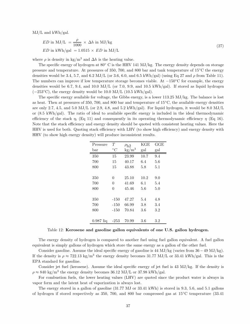
MJ/L and kWh/gal.
ED in MJ/L =ρ
1000× ∆h in MJ/kg
ED in kWh/gal = 1.0515 × ED in MJ/L(27)
where ρ is density in kg/m3 and ∆h is the heating value.The specific energy of hydrogen at 80 C is the HHV 141 MJ/kg. The energy density depends on storage
pressure and temperature. At pressures of 350, 700, and 800 bar and tank temperature of 15C the energydensities would be 3.4, 5.7, and 6.2 MJ/L (or 3.6, 6.0, and 6.5 kWh/gal) (using Eq 27 and ρ from Table 11).The numbers can improve if low temperature storage becomes viable. At −150C for example, the energydensities would be 6.7, 9.4, and 10.0 MJ/L (or 7.0, 9.9, and 10.5 kWh/gal). If stored as liquid hydrogen(−253C), the energy density would be 10.0 MJ/L (10.5 kWh/gal).
The specific energy available for voltage, the Gibbs energy, is a lower 113.25 MJ/kg. The balance is lostas heat. Then at pressures of 350, 700, and 800 bar and temperature of 15C, the available energy densitiesare only 2.7, 4.5, and 5.0 MJ/L (or 2.9, 4.8, and 5.2 kWh/gal). For liquid hydrogen, it would be 8.0 MJ/Lor (8.5 kWh/gal). The ratio of ideal to available specific energy is included in the ideal thermodynamicefficiency of the stack ηi (Eq 11) and consequently in its operating thermodynamic efficiency η (Eq 16).Note that the stack efficiency and energy density should be quoted with consistent heating values. Here theHHV is used for both. Quoting stack efficiency with LHV (to show high efficiency) and energy density withHHV (to show high energy density) will produce inconsistent results.
Pressure T ρh2 KGE GGEbar C kg/m3 gal gal
350 15 23.99 10.7 9.4700 15 40.17 6.4 5.6800 15 43.88 5.8 5.1
350 0 25.10 10.2 9.0700 0 41.69 6.1 5.4800 0 45.46 5.6 5.0
350 -150 47.27 5.4 4.8700 -150 66.99 3.8 3.4800 -150 70.84 3.6 3.2
0.987 liq -253 70.99 3.6 3.2
Table 12: Kerosene and gasoline gallon equivalents of one U.S. gallon hydrogen.
The energy density of hydrogen is compared to another fuel using fuel gallon equivalent. A fuel gallonequivalent is simply gallons of hydrogen which store the same energy as a gallon of the other fuel.
Consider gasoline. Assume the ideal specific energy of gasoline is 44 MJ/kg (varies from 36−49 MJ/kg).If the density is ρ ≈ 722.13 kg/m3 the energy density becomes 31.77 MJ/L or 33.41 kWh/gal. This is theEPA standard for gasoline.
Consider jet fuel (kerosene). Assume the ideal specific energy of jet fuel is 43 MJ/kg. If the density isρ ≈ 840 kg/m3 the energy density becomes 36.12 MJ/L or 37.98 kWh/gal.
For combustion fuels, the lower heating values (LHV) are quoted since the product water is always invapor form and the latent heat of vaporization is always lost.
The energy stored in a gallon of gasoline (31.77 MJ or 33.41 kWh) is stored in 9.3, 5.6, and 5.1 gallonsof hydrogen if stored respectively as 350, 700, and 800 bar compressed gas at 15C temperature (33.41
37

kWh of energy ÷ 3.6, 6.0, and 6.5 kWh/gal of hydrogen); or in 3.2 gallons of hydrogen if stored as liquid(33.41 ÷ 10.5). These are the gasoline gallon equivalents (GGE). Similarly, the energy stored in a gallon ofkerosene (36.12 MJ/L or 37.98 kWh/gal) is stored in 10.7, 6.4, or 5.8 gallons of hydrogen under the samepressures and temperature (37.98 kWh of energy ÷3.6, 6.0, and 6.5 kWh/gal of hydrogen); or in 3.6 gallonsof hydrogen when stored as liquid. This would be the kerosene gallon equivalent (KGE).
So a fuel gallon equivalent (FGE) is gallons of hydrogen given by
FGE =EDfuel × 1 gallon
EDh2=
ρfuelρh2
∆hfuel∆hh2
× 1 gallon (28)
where ρ is density and ∆h is the specific energy or heating value.Table 12 lists the kerosene and gasoline gallon equivalents. The numbers are generated using: ∆hh2 =
141 MJ/kg (HHV of hydrogen at 80 C), ρker = 840 kg/m3 and ∆hker = 43 MJ/kg for kerosene, andρgas = 722.13 kg/m3 and ∆hgas = 44 MJ/kg for gasoline. Only ρh2 varies with pressure and temperature(third column). If stored at 700 bar and 15 C, 6.4 gallons of hydrogen are needed for every gallon ofkerosene, and 5.6 gallons of hydrogen for every gallon of gasoline.
The true fuel gallon equivalent (FGE true) is found by including engine efficiency in the definition.
FGE true =ρfuelρh2
∆hfuel∆hh2
ηfuelηh2
× 1 gallon (29)
Figure 17 shows commercial and experimental automobile tank data for 350 bar, 450 bar, 700 bar andliquid storage for 5 − 10 kg of hydrogen. The weight fraction is defined as weight of hydrogen at full tank÷ weight of tank system including hydrogen. A weight fraction of 5% means 5 kg of hydrogen needs 100kg of tank system including the hydrogen. This data was collected in 2014 and some products no longerexist. The average still remains at 5.5% or so, for 5 kg of storage, due to the requirement to prevent boil-offover days and weeks. The fraction is expected to improve with higher amounts of storage. Figure 18 givesextreme examples. But it is really short-term storage, where boil-off can be allowed, that might enablehigher fractions. The Navy Ion Tiger demonstrated 13% with only 0.5 kg of hydrogen (liquid) using theshort term nature of storage. There is a gap in test data for the amount of hydrogen envisioned for eVTOL(10 − 20 kg) and the amount of storage time envisioned for eVTOL (1 − 3 hr) for a definitive conclusion.
6.5 Air flow
Air flows into the cathode and carries with it oxygen needed for the reaction. Let the mass flow rate of air bewAir in kg/s and the oxygen needed be wO kg/s. Non-reacting gases (mainly nitrogen) and excess oxygenleave as exhaust. Let this rate be wAir out. Water is generated inside the stack at a rate of wW = wO + wH .This water also leaves as exhaust.
The cathode should be humidified, but not flooded. Water and humidity management in the cathode iscomplex. In general, the total water exhaust contains the product water generated and water transportedfrom anode to cathode through the membrane. A part of the water generated can be humidified and passedback into the anode and cathode to keep the electrodes and membranes hydrated. Then, water vapor alsoenters the cathode. Water production, transport, and balance are affected by intricate mechanisms inside afuel cell. Modeling these mechanisms are important for stack design but not aircraft design. In the presentmodel, only the product water is considered. So the model is simple; the input to the cathode is wAir in andthe outputs are wAir out and wW . The product water is either vapor or liquid, if the output air is saturatedwith vapor. Regardless of simplicity, the mass flow rate across the stack must be conserved.
38
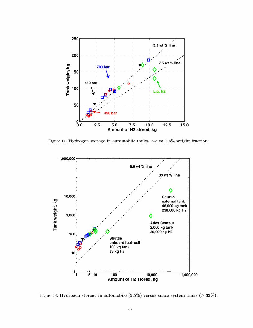
0.0 2.5 5.0 7.5 10.0 12.5 15.00
50
100
150
200
250
Amount of H2 stored, kg
Tank
wei
ght,
kg
350 bar
Liq. H2
700 bar
450 bar
5.5 wt % line
7.5 wt % line
Figure 17: Hydrogen storage in automobile tanks. 5.5 to 7.5% weight fraction.
1 5 10 100 10,000 1,000,0001
10
100
1,000
10,000
1,000,000
Amount of H2 stored, kg
Tank
wei
ght,
kg
Shuttle onboard fuel−cell100 kg tank33 kg H2
Atlas Centaur2,000 kg tank20,000 kg H2
Shuttle external tank46,000 kg tank230,000 kg H2
5.5 wt % line
33 wt % line
Figure 18: Hydrogen storage in automobile (5.5%) versus space system tanks (≥ 33%).
39

The conservation of mass across the stack is described as follows.
(input) wH + wAir in =wH + wO + wAir out=wW + wAir out=wW liq + wW vap + wAir out (output)
(30)
The mass flow rate of air is calculated from the mass flow rate of oxygen. The mass flow rate of oxygenis obtained from the cathode half reaction
1/2 O2 + 2e− + 2H+ → H2O Cathode, capture of electrons, reduction (31)
Let SO moles of oxygen capture the N moles of electrons in the cathode arriving from the anode half reaction.Here SO = 1/2 and N = 2. (One mole of oxygen captures N/SO = nC = 4 moles of electrons at the cathodewhich was used during the construction of the i − v curve earlier.)
Since a mole of electron carries a charge of F Coulomb (F = 96485 Coulomb/mole is the Faraday’sconstant), N moles of electrons carry NF Coulomb. So SO moles of oxygen are needed to capture NFCoulomb. If one mole of oxygen weigh mO kg, SO moles of oxygen weigh SOmO kg. So SOmO kg of oxygenis needed to capture NF Coulomb. Or 1 Coulomb is captured by SOmO/NF kg of oxygen. So I Ampere(Coulomb/s) is captured by ISOmO/NF kg/s of oxygen. The current I must be captured in every cell sothe total consumption is found by multiplying the number of cells nc.
Thus, the mass flow rate of oxygen is
wO = SOmO
N FI nc (32)
where wO is the mass flow in kg/s, nc is the number of cells, I is the current in Ampere, N = 2, F = 96485Coulomb/mole, mO = 31.9988× 10⁻³ kg/mole is the molecular weight of oxygen, and SO = 1/2.
The mass flow rate of air is then
wAir = SOmA
xO N FI nc (33)
where wAir is the mass flow in kg/s and xO = 0.2095 is the mole fraction of oxygen in air.If supply rate is greater than consumption SO is multiplied with an utilization factor fA.
wAir in = fA SOmA
xO N FI nc (34)
Typically, fA ≈ 1.5 − 2.5 for PEMFC.From Eq (2), I nc = P nc/V = P/v, so it can also be written as
wAir in = fA SOmA
xO N F
P
v(35)
which shows it is proportional to power but varies inversely with cell voltage. A higher cell voltage requireslower air flow for the same power.
The volume flow rate of air is
vAir in =wAir in
mA
R T
p(36)
where vAir in is the volume flow of air in m3/s, p is stack pressure in Pa, R = 8.3144621 J/mol.K is theuniversal gas constant, T is the stack temperature in K, mA = 28.9655 × 10⁻³ kg/mole is the molecularweight of dry air, and wAir in is the mass flow in kg/s. The fraction R/mA = 287 J/kg-K is the specific gasconstant of dry air.
40

The volume flow rate in cubic feet per minute (CFM) is often used.
CFM = 4.72 × 10⁻⁴ × vAir in (37)
At the design point, I = ID, P = PD, v = vc.At the maximum power point: I = Ipmax, P = Pmax, v = vpmax.The air flow out is air flow in minus the oxygen consumed.
wAir out = wAir in − wO (38)
The product water is the hydrogen plus oxygen consumed.
wW = wH + wO (39)
The vapor and liquid content can be estimated from the humidity ratio. The saturation pressure of watervapor, pWs, is calculated using the empirical Arden Buck equations (Buck 1981; revised 1996).
α =
(
18.678−C
234.5
) ( C
257.14 + C
)
pWs = 611.21 eα
(40)
where C is the stack output temperature and pWs is the pressure in Pa.The maximum saturation humidity ratio is
hs =mW
mA
pWs
p − pWs= 0.622
pWs
p − pWs(41)
where mW = 18.0153 × 10⁻³ kg/mole is the molecular mass of water, mA = 28.965 × 10⁻³ kg/mole is themolecular mass of air, and p is the stack output pressure. p = pS − ∆pS . pS is the stack inlet pressure and∆pS is a specified stack pressure drop. ∆pS ≈ 20 − 50 kPa for a 80 kWe stack.
If hs wAir out ! wW , the product water is in vapor form.Then
wW vap = wW
wW liq = 0(42)
In this case less water is produced than what the air can hold. A cathode humidifier will be needed.If hs wAir out < wW , the product water is partially liquid after air saturation with vapor.Then
wW vap = hs wAir outwW liq = wW − wW vap
(43)
In this case more water is produced than what the output air can hold. A cathode humidifier will not beneeded. A prescribed fraction f of wW liq is stored on-board.
41

7 Balance of Plant
The power to operate the subsystems is the balance of plant (BOP) PBOP . This section describes thecalculation of power for air supply, hydrogen supply, cooling systems, water system, and the electricalsystem.
Power generated (kW) minus BOP is the net electrical power (kWe). Normally, air supply consumesthe most power, but power is also needed to supply fuel, circulate coolants, pump water, and operate thecontroller and other power electronics.
PBOP = PAir + PFuel + PLtc + PHtc + PWater + PElec (44)
Power is calculated in Watts in the following form.
P = dP + Pmodel (45)
where Pmodel is the model prediction and dP an user specified increment. Because there is no historicaldata base, the model uses elementary theory and scaling laws of the form k Xe where X is the principalscaling variable and k and e are calibration constants from data or higher fidelity analysis. dP can be usedto specify losses directly with k = 0.
Air supply
The air supply loss is from a blower or pump or a compressor-expander.The power of a blower or pump is calculated as
Pblower = ∆p vAir in/η
Pblower max = ∆p vAir in max/η(46)
where ∆p = pS − pa is the difference between the stack pressure and atmospheric pressure in Pa, v is thevolume flow rate in m3/s (Eq 36), and η is the efficiency. A blower can be used up to ∆p ≈ 30 kPa, a pumpup to ≈ 100 kPa (stationary), but for higher pressures a compressor is needed.
The power of a compressor is
Pcomp = Cp wAir in ∆T
Pcomp, max = Cp wAir in max ∆T(47)
where Cp is specific heat of air in J/kg-K, w is the inlet air flow in kg/s, and ∆T is the rise in temperature inthe compressor in K. If the input and output temperatures and pressures are T1 and P1, and T2 and P2 respec-tively, then the ideal (minimum) power is obtained for isentropic compression when T2 = T1 (P2/P1)(γ−1)/γ
where γ is the ratio of specific heat. An efficiency η accounts for non-ideal compression and other mechanicallosses. Typically η ≈ 0.7 − 0.8.
∆T =
[(
P2
P1
) γ−1
γ
− 1
]
T11
η(48)
42
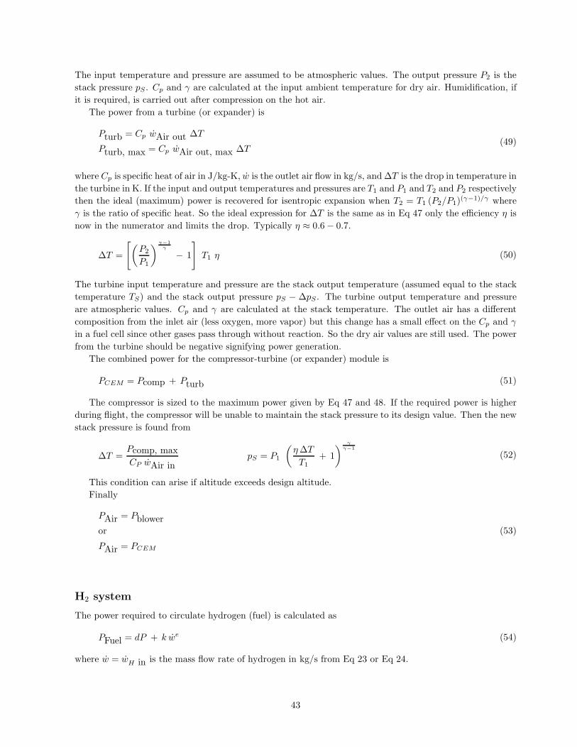
The input temperature and pressure are assumed to be atmospheric values. The output pressure P2 is thestack pressure pS . Cp and γ are calculated at the input ambient temperature for dry air. Humidification, ifit is required, is carried out after compression on the hot air.
The power from a turbine (or expander) is
Pturb = Cp wAir out ∆T
Pturb, max = Cp wAir out, max ∆T(49)
where Cp is specific heat of air in J/kg-K, w is the outlet air flow in kg/s, and ∆T is the drop in temperature inthe turbine in K. If the input and output temperatures and pressures are T1 and P1 and T2 and P2 respectivelythen the ideal (maximum) power is recovered for isentropic expansion when T2 = T1 (P2/P1)(γ−1)/γ whereγ is the ratio of specific heat. So the ideal expression for ∆T is the same as in Eq 47 only the efficiency η isnow in the numerator and limits the drop. Typically η ≈ 0.6 − 0.7.
∆T =
[(
P2
P1
) γ−1
γ
− 1
]
T1 η (50)
The turbine input temperature and pressure are the stack output temperature (assumed equal to the stacktemperature TS) and the stack output pressure pS − ∆pS . The turbine output temperature and pressureare atmospheric values. Cp and γ are calculated at the stack temperature. The outlet air has a differentcomposition from the inlet air (less oxygen, more vapor) but this change has a small effect on the Cp and γin a fuel cell since other gases pass through without reaction. So the dry air values are still used. The powerfrom the turbine should be negative signifying power generation.
The combined power for the compressor-turbine (or expander) module is
PCEM = Pcomp + Pturb (51)
The compressor is sized to the maximum power given by Eq 47 and 48. If the required power is higherduring flight, the compressor will be unable to maintain the stack pressure to its design value. Then the newstack pressure is found from
∆T =Pcomp, maxCP wAir in
pS = P1
(η ∆T
T1+ 1
) γγ−1
(52)
This condition can arise if altitude exceeds design altitude.Finally
PAir = Pbloweror
PAir = PCEM
(53)
H2 system
The power required to circulate hydrogen (fuel) is calculated as
PFuel = dP + k we (54)
where w = wH in is the mass flow rate of hydrogen in kg/s from Eq 23 or Eq 24.
43

High temperature cooling system
The high temperature cooling system refers to the stack cooling system. The nomenclature follows theDOE HP. The nomenclature is generic since it is not essential a liquid cooling system be part of the model.Normally, a liquid cooling system is needed for stacks of power > 10 kW. The distinction between high andlow temperature coolants is also formal since often the same coolant is used to circulate in both systems —the stack and the air. Other nomenclatures are also used in literature such as the inner and outer coolingsystems. The model developed is conceptual and broadly applicable to all.
The Heat Ventilation and Air Conditioning (HVAC) system of the vehicle is ignored so refrigerant andcondensers are not included in the model. It is assumed these are already dealt as in any conventionalaircraft with cabin air and not strictly a part of the propulsion system.
The power required to circulate the coolant is calculated as
PHtc = dP + k Qe wf (55)
where Q in Watts is the net heat to be rejected and w = wc in kg/s is the coolant mass flow rate. For aircooled systems, there is no coolant, and the exponent f = 0. The Q and w are calculated as follows.
The total stack heat is
Qstack = (Eh − v) i Anc = (Eh − v) iP
p= (Eh − v)
P
v=
(1/η − 1
)
P (56)
where Eh is the higher heating value and η = v/Eh. The higher heating value provides a conservativeestimate by including conditions under which liquid water forms in the stack releasing the latent heat ofcondensation. This estimate can be too conservative, in which case the lower heating value can be used.
The maximum heat is at the maximum power
Qstack max = (Eh − vpmax) ipmax Anc =(
1/η|pmax − 1)
Pmax (57)
where η|pmax = vpmax/Eh. If the maximum heat is deemed too high, the design heat can be used forsizing. Then the maximum power is not continuous power and must be rated.
If there is no compressor, a part of the stack heat can be used to heat the inlet air.
Qin = Cp wAir in ∆T (58)
where Cp is the specific heat of air J/kg-K at the ambient temperature, w is the mass flow rate of air in kg/s(Eq 34), and ∆T is the difference in temperature between the stack and the ambient.
A part of the heat is carried out by the air
Qout = Cp wAir out ∆T (59)
where Cp is the specific heat of air J/kg-K at the stack temperature, w is the mass flow rate of air in kg/s(Eq 38), and ∆T is the difference in temperature between the stack and the ambient. The input stoichiometry(fA SO in Eq 34) is a key variable that affects this heat.
A part of the heat is dissipated.The dissipated heat can be specified as a fraction of the total stack heat
Qd = fd Qstack (60)
or calculated from natural convection (Qc) and radiation (Qr) losses from the stack exposed surface area.
Qd = Qc + Qr
Qc = As h (TS − Ta)
Qr = As ϵ σ(
T 4S − T 4
a
)
(61)
44

The area As is the stack exposed surface area specified as a fraction of stack active area.
As = fs nc Ac (62)
The coefficient h is the overall convection heat transfer coefficient in W/m2K, TS is the stack temperature inK, Ta is the ambient temperature in K as seen by the stack (atmospheric ambient or the enclosure), ϵ is theemissivity of the stack (non-dimensional ≈ 0.8), and σ = 5.670367× 10⁻⁸ W/m2K4 is the Stefan-Boltzmannconstant. The coefficient h is difficult to calculate and assumed to be an input from a more detailed heatanalysis that considers air flow over the stack. It is typically in the range 10 − 100 W/m2K. If these detailsare not available the fraction fd can be specified instead. For very small stacks (≈ 10 − 50 W) fs can be sohigh that cooling is not a problem at all, and a heater might be needed instead to raise the stack temperature.
The net heat to be rejected is the balance
Q = Qstack − Qin − Qout − Qd (63)
The cooling system is a pumped loop circulating a coolant which collects the heat (by flowing throughthe cells or by other means) to a radiator which rejects it to the atmosphere.
The mass flow rate of the coolant is found from
Q = Cp wc ∆Tc (64)
where Cp is the specific heat of the coolant in J/kg-K at the coolant temperature, wc is the mass flow rateof the coolant in kg/s, and ∆Tc is the rise in coolant temperature as it absorbs stack heat. ∆Tc < 15 C.The coolant inlet and outlet temperatures are then assumed to be TS − ∆Tc and TS respectively.
The difference in temperature between the stack coolant outlet temperature (assumed equal to the stacktemperature TS) and the ambient temperature of the radiator Ta is an important parameter ∆T . The ambienttemperature is the maximum temperature for which the system is still be able to reject the heat. The ratioQ/∆T is a heat rejection parameter that has been found useful in automobile fuel cells to optimize stacktemperature and efficiency. Q/∆T < 1.45 kW/C is a target for automobile stacks of 80-kWe with ambientheat rejection temperature of Ta = 40C. In the present model, Ta is specified and Q/∆T is calculated.
Medium Specific Density Thermal Boiling Freezingheat conductivity point point
kJ/kg-K kg/m3 W/m K C C
Water 4.18 995 0.65 100 0
50-50 3.28 1082 0.40 107 -37Water/Ethylene Glycol
50-50 3.56 1010 0.36 106 -45Water/Propylene Glycol
Table 13: Properties of typical coolants.
Table 13 shows typical liquid coolants. The cooling channels are usually built into the bipolar plates ofthe cells. A deionizer is used to prevent the coolant from becoming conductive due to ion contaminationfrom the bipolar plates. An electrically conductive coolant leads to high leakage current which reduces cellefficiency. Antioxidants are also used for the same purpose. In addition, corrosion inhibitors are also used.So the properties are modified from the nominal water/Glycol values in Table 13 and should be specifiedaccordingly.
45

The radiator rejects heat by convection (Qc) and radiation (Qr) from the radiator surface area.
Q = Qc + Qr
Qc = Ar h (Tr − Ta)
Qr = Ar ϵ σ(
T 4r − T 4
a
)
(65)
The area Ar is the radiator surface area in m2 that is to be calculated. The coefficient h is the overallconvection heat transfer coefficient in W/m2K, Tr is a specified radiator temperature in K, ϵ is the emissivityof the stack (non-dimensional), and σ = 5.670367× 10⁻⁸ W/m2K4 is the Stefan-Boltzmann constant. Thecoefficient h is difficult to calculate and assumed to be an input from a more detailed heat analysis thatconsiders air flow over the radiator. The coefficient h = Nu k/D where Nu is the Nusselt number (non-dimensional), k is the thermal conductivity in W/m K, and D is the hydraulic diameter. Nu depends onnatural or forced convection, laminar or turbulent flow, and the Prandtl, Reynolds, and Rayleigh numbers(Nu = 1 for pure conduction, ≈ 10 for laminar flow, and ≈ 100 − 1000 for turbulent flow). Other inputsare the radiator temperature Tr (≈ 100C), ϵ (≈ 0.7 − 0.8), and the ambient temperature Ta for which thesystem should still be able to reject heat. The final output is the radiator area Ar from which the weightand volume can be calculated.
Low temperature cooling
The power required to circulate the coolant is calculated as
PLtc = dP + k Qe wf (66)
where Q in Watts is the heat to be rejected and w = wc in kg/m is the coolant mass flow rate. For aircooled systems (no coolant) the exponent f = 0. The heat Q and coolant mass flow rate w are calculated asfollows.
Q = Cp wAir in ∆T (67)
where Cp is the specific heat of air J/kg-K at the compressor output temperature, w is the mass flow rate ofair in kg/s (Eq 34), and ∆T is the difference in temperature between the compressor output and the stacktemperature in K.
The cooling system is a pumped loop circulating a coolant which collects the heat (by flowing throughthe cells or by other means) to a radiator which rejects it to the atmosphere.
The mass flow rate of the coolant is found from
Q = Cp wc ∆Tc (68)
where Cp is the specific heat of the coolant J/kg-K at the coolant temperature, wc is the mass flow rate ofthe coolant in kg/s, and ∆Tc is the rise in coolant temperature. ∆Tc < 15 C.
The heat rejection in the radiator follows the same theory as high temperature cooling. If the sameradiator is used, only one should be modeled by using k = 0 for the other.
Water system
The power required to circulate the water is
PWater = dP + k we (69)
where w = wW liq is the maximum liquid water rate in kg/m (Eq 43 or, for a conservative estimate, Eq 39).
46

Electrical system
The power required for the electrical system is
PElec = dP + k P e (70)
where P = Pmax is the maximum stack power in Watts.
47

8 Weights
This section describes the calculation of weights, although by weight, really mass is meant.The total weight consists of the weight of the stack, air supply, hydrogen (fuel), tank, cooling systems,
water system, and the electrical system.
W = WStack + WAir + WFuel + WTank + WLtc + WHtc + WWater + WElec (71)
Weight (mass) is calculated in kg in the following form.
W = dW + Wmodel (72)
where Wmodel is the model prediction and dW is an user specified increment. Because there is no historicaldata base, the models use elementary theory and scaling laws of the form k Xe where X is the principalvariable and k and e are calibration constants from data or higher fidelity analysis. dW can be used tospecify weights directly with k = 0.
Volume is calculated in m3 in the same manner
S = dS + Smodel (73)
Stack
If the stack power is P , and the cell power density is p, the membrane area must be P/p since p is thepower produced per unit area. If the weight is assumed to be proportional to this area: W ∝ P/p, then theconstant of proportionality is a ratio of cell power density and stack power to weight.
κ =p
P/W (74)
This ratio is a text-book design factor. It has dimensions of mass per area and unit of kg/m2. It varies onlywith materials and mechanical construction of the stack. It ranges from 4 − 20 kg/m2 with lower values forbetter stacks. As an example, if the design factor is 5 kg/m2, then cells of power density pc = 0.5 W/cm2
(= 5 kW/m2) would produce a stack of P/W = 1.0 kW/kg. If superior cells of pc = 1 W/cm2 (= 10 kW/m2)can be found, a lighter stack of P/W = 2.0 kW/kg can be built.
The stack power P = Ac nc p from Eq 2, hence the design factor is
κ =W
nc Ac(75)
which is how it is calculated.The weight of a stack is calculated part by part. Figure 19 gives a diagram of the main parts of a
typical fuel cell which is the basis for the present model. For detailed topology and fabrication processes andmaterials of modern cells, see De Las Heras et al 2018.
The weight of the proton exchange membrane (PEM) is
Wpem = Ac tpem ρpem (76)
where W is the weight in kg, Ac is the cell active area in m2 (the area covered by the catalysts), ρ is densityin kg/m3, and t is thickness in m.
48

Figure 19: Parts of a typical fuel cell.
Figure 20: Parts of a typical fuel stack.
49

The membrane electrode assembly (MEA) is the membrane sandwiched between a pair of gas diffusionlayers (GDL) and then sealed with gaskets. The GDL have the same area as the active area. The sealinggaskets occupy a small fraction of this area given by the factor k. The weight of the MEA is
Wmea = Wpem + 2 Ac tgdl ρgdl + 2 kseal Ac tseal ρseal (77)
The cell is the MEA sandwiched between a pair of bipolar plates. The bipolar plates contain channelsthrough which reactants (air on cathode and hydrogen on anode side) and coolants flow. The channels canbe of many designs. The non-dimensional porosity φ accounts for them at a gross level. The weight of thecell is
Wcell = Wmea + 2 kbp Ac tbp ρbp φbp (78)
The unit is the collection of cells
Wunit = nc Wcell (79)
The stack is the unit sandwiched between current collectors, insulating layers, and end plates, all tiedtogether by a fastener. Figure 20 shows the parts of a typical stack. The stack weight is
WStack = Wunit +∑
2 k Ac t ρ + Wfas + Wother (80)
where the summation is over the collector plates (cp), insulating plates (ip), and end-plates (ep) with theirrespective area fraction, thickness, and density. The weight of the fastener is an input since they vary widelyfrom basic steel bolts and clamps to lighter composite wraps. The other weights cover for missing items inthe model.
In general, the weight is proportional of the active area times the number of cells, plus an overhead. SinceAc = P/(nc p), the weight is simply proportional to the design power P divided by the cell power density p.
WStack = k0 + k1P
p(81)
The constants k0 and k1 vary only with construction technology and materials.The length of the stack is
Lstack = tc +∑
2 t (82)
where the summation is over the gdl, seal, bp, cp, ip, and ep. The thickness and length are in m.The cross-sectional area of the stack (m2) is the area of the end-plate.
Astack = Aep = kep Ac (83)
The volume of the stack (m3) is
Sstack = Lstack Astack (84)
An equivalent cell thickness (m) is calculated by dividing stack length with number of cells.
tcell =Lstack
nc(85)
An equivalent cell density (kg/m3) is calculated by specifying a porosity φstack (non-dimensional)
ρcell =Wstack − Wfas − Wother
Lstack Ac φstack(86)
50

The equivalent cell thickness and density make up the simplest weight model
WStack = ρcell tcell nc Ac φstack + Wfas + Wother (87)
For this model Lstack = tcell nc and Astack = Ac.Either Eq 80 or Eq 87 can be used to calculate the stack weight.The design factor is then found using Eq 75 and Eq 81
κ =WStacknc Ac
=k0
P/p+ k1 (88)
where k0 is from the overhead of Wfas and Wother. It can dominate small low power stacks < 1 kW, andproduce a poor (high) design factor even with good electrochemistry.
Fuel system
The fuel system supplies hydrogen to the stack. The weight model consists of hydrogen and the tank.
WFuel =Wh2 + Wtank (89)
There is no real model of the tank, just specified fractions, which are adequate for the conceptual natureof the design.
The gravimetric weight fraction of hydrogen storage wf is defined as the weight of a full tank of hydrogendivided by the weight of hydrogen and tank system combined.
wf =Wh2
Wh2 + Wtankwt % = wf × 100 (90)
Thus the weight of hydrogen and tank system is
Wh2 + Wtank =Wh2wf
(91)
and the tank alone is
Wtank =1 − wf
wfWh2 (92)
The system gravimetric capacity or net specific energy of storage is
∆hh2 tank = wf ∆hh2 (93)
The specific energy of hydrogen is ∆hh2 = 141 MJ/kg (HHV) or 120 MJ/kg (LHV). But 1 kg of hydrogenrequires 1/wf kg of tank system. Thus the net specific energy is wf × 141 (HHV) or wf × 120 (LHV). For 6wt% the net specific energy is 8.5 MJ/kg (HHV) or 7.2 MJ/kg (LHV), or 2.35 kWh/kg (HHV) or 2 kWh/kg(LHV). This value should not be compared with batteries; the weight of the fuel stack should be includedfor any comparison since batteries combine the engine and the fuel. In fact a battery also carries its oxidizerwhich contributes to both its high compactness and heavy weight.
A volume fraction is defined similarly, except the tank volume automatically includes the hydrogen.
sf =Sh2
Stank(94)
Thus the tank volume is
Stank =Sh2sf
(95)
51

The volume of hydrogen is related to the hydrogen weight and density at full tank.
Stank =Wh2
ρh2 sf(96)
A tank volume overhead factor can also be defined for volume
sov =Stank − Sh2
Stank= 1 − sf (97)
Thus alternatively, the tank volume is
Stank =Wh2
ρh2 (1 − sov)(98)
The weight of hydrogen divided by the volume of the tank is the storage density.
ρh2 store =Wh2Stank
= ρh2 sf = ρh2 (1 − sov) (99)
The storage density is also called the volumetric weight fraction in literature.The weight fraction wf and storage density ρh2 store are typical model inputs. The storage density
makes it easy and intuitive to calculate the tank volume Stank from weight of hydrogen Wh2. But thestorage density must be lower than hydrogen density otherwise non-physical results are produced. Since thehydrogen density is a function of temperature and pressure, this is not easy to track. The tank overheadfactor sov is a safer and the preferred input. Results are always physically meaningful for sov > 0.
Air supply system
The air supply to the stack consists of a blower (or compressor and turbine) and a humidifier. Provisionsare also kept for filters, regulators, power supply, and plumbing. A power supply might be needed forhumidification or for cold-start.
WAir =Wblower + Wcomp + Wturb + Whumidifier +
Wfilter + Wregulator + Wpower + Wplumbing(100)
The weights and volumes of the blower, compressor, and turbine are scaled to the maximum mass flowrate (kg/s) and power with specified constants and exponents.
W or S = k we P f (101)
where k, e, and f are input separately for each component, w is the maximum mass flow rate (kg/s) and Pis the maximum power (W).
For the blower or the compressor, w is maximum mass flow rate of air input; for the turbine, w is themaximum mass flow rate of air output.
w = wAir in, max blower or compressor
w = wAir out, max turbine(102)
For stacks of power < 100 kW, an axial-flow turbine (expander) is typically integrated into a singlecompressor-expander unit. Then only one sizing model can be used.
52

The weight of the humidifier, cooler, filter, regulator, and power are simply fractions of total weight ofthe air supply system
W = dW + f WAir (103)
The weight of the plumbing is given by
W = dW + wl (104)
where w is the weight per length (kg/m) and l is the length of plumbing (m).
High temperature cooling system
A high temperature cooling system cools the stack. The weight model consists of a radiator and coolant. Acooler is not needed as the purpose is to simply remove the heat. Provisions are kept for filters, regulators,power supply (to circulate the coolant), and plumbing.
WHtc =Wcoolant + Wradiator +
Wfilter + Wregulator + Wpower + Wplumbing(105)
The weight of the coolant is proportional to the heat rejected or coolant mass flow rate.
Wcoolant = dW + k Qe wfc (106)
where W is the weight in kg, dW is an increment, k, e and f are input parameters, Q is heating in Wattfrom Eq 63, and wc is the coolant mass flow from Eq 64. For e = 0 and f = 1, k is time in seconds givestotal mass of coolant k w in kg.
The weight of the radiator is scaled to the heat rejected or the radiator area.
Wradiator = dW + k Qe Afr (107)
where W is the weight in kg, dW is an increment, k and e are input parameters, and Q is heating in W fromEq 63, and Ar is the radiator area in m2 from Eq 65. If there is no radiator f = 0. If there is a radiatorf = 1 and k is the radiator weight per area in kg/m2. Typical values can range from 3 − 8 kg/m2.
The volume of the radiator is accounted for in the same manner as the weight
Sradiator = dS + k Qe Afr (108)
where S is volume in m3, dS is an increment, and k and e are input parameters. If there is no radiatorf = 0. If there is a radiator f = 1, and k is the radiator thickness in m.
The radiator can be a very heavy component and a major weight overhead. Determining the factorsrequire detailed design that takes advantage of the application environment.
The weight of the filter, regulator, and power are simply input fractions of total weight of the coolingsystem
W = dW + f WHtc (109)
The weight of the plumbing is given by
W = dW + wl (110)
where w is the weight per length (kg/m) and l is the length of plumbing (m).
53

Low temperature cooling system
If a compressor is used, and the compression ratio is high, the output air is at a high temperature. A lowtemperature cooling system is required to cool the air before it enters the stack. The weight model consistsof a cooler, coolant, and a radiator. Provisions are kept for filters, regulators, power supply (to circulate thecoolant), and plumbing.
WLtc =Wcooler + Wcoolant + Wradiator +
Wfilter + Wregulator + Wpower + Wplumbing(111)
The weight of the cooler is scaled to the heat rejected.
Wcooler = dW + k Qe (112)
where W is weight in kg, dW is an increment, k is an input parameter, and Q is heating from Eq 67.The weight of the coolant is scaled to the heat rejected or the coolant mass flow rate.
Wcoolant = dW + k Qe wfc (113)
where W is the weight in kg, dW is a prescribed weight, k, e and f are input parameters, Q is heating fromEq 67 and wc is the coolant mass flow from Eq 68. For e = 0 and f = 1, k is time in seconds gives totalmass of coolant k w in kg.
The weight of the radiator is scaled to the heat rejected or the area.
Wradiator = dW + k Qe Afr (114)
where W is the weight in kg, dW is a prescribed weight, k, e and f are input parameters, and Q is heatingin W from Eq 67, and Ar is the radiator area in m2. If there is no radiator f = 0. If there is a radiatorf = 1 and k is the radiator weight per area in kg/m2. Typical values can range from 3 − 8 kg/m2.
The volume of the radiator is accounted for in the same manner as the weight
Sradiator = dS + k Qe Afr (115)
where S is volume in m3, dS is a prescribed volume in m3, and k, e, and f are input parameters. If there isno radiator f = 0. If there is a radiator f = 1 and k is the radiator thickness in m.
The weight of the filter, regulator, and power are prescribed as fractions of total weight of the coolingsystem
W = dW + f Wltc (116)
The weight of the plumbing is given by
W = dW + wl (117)
where w is the weight per length (kg/m) and l is the length of plumbing (m).
Water system
The water system model is just a storage tank with provisions for filters, regulators, power supply (to pump),and plumbing.
WWater =Wtank +
Wfilter + Wregulator + Wpower + Wplumbing(118)
54

The weight of water stored is
W = f t wW liq (119)
where f is the fraction of water produced by the stack over a time t at a rate w. The fraction f and time tare specified inputs.
The weight and volume of the tank are
Wtank = (1 + wov) W
Stank = (1 + sov) W/ρ(120)
where the fractions wov and sov are specified and ρ is the density of water.The weight of the filter, regulator, and power are input fractions of total weight of the water system.
W = dW + f WWater (121)
The weight of the plumbing is given by
W = dW + wl (122)
where W is the weight per length (kg/m) and l is the length of plumbing (m).
Electrical system
The electrical system model consists of a controller with provisions for power electronics and plumbing(wiring).
WElec =Wcontroller + Wpower + Wplumbing (123)
The weight of the controller is scaled to the maximum stack current.
Wcontroller = dW + k Ie (124)
where dW , k and e are inputs and I = Ipmax.The weight of power electronics is simply input fraction of total weight of the electrical system.
Wpower = dW + f WElec (125)
The weight of the plumbing is given by
W = dW + wl (126)
where w is the weight per length (kg/m) and l is the length of wiring (m).
55

9 Software Overview
The software is written in MATLAB.The src directory contains the following source files.
createiv.m Creates i − v.
DATA gptX.m Gas phase thermochemistry data.
X=H2, O2, H2Ol (liq water) and H2Ov (vapor).
DATA DryAirCp.m Air Cp and γ.
h2density.m Density of compressed hydrogen.
ISAtmosphere.m Atmospheric model up to 11 km.
ivpolarization.m Uses i − v. Applies corrections.
pemfc.m Designs system for a specified power kW.
pemfcdesign.m Designs system for a specified net power kWe.
Iterates pemfc.m.
pemfcstatic.m Analyzes a design.
watervp.m Saturated vapor pressure of water.
The following run directories are provided.run Baseline 80kW
run Modern 80kW
run Modern 80kW liqcool
run Modern 500kW liqcool
run Modern 500kW liqcool P1.0
Each run directory contain the following files.
Input-output file
fcvariables.m Lists all inputs and outputs.
Outputs set to zero.
Drivers for design
drivercreativ.m Fits model to i − v data.
driverpemfc.m Executes pemfc.m
driverpemfcdesign.m Executes pemfcdesign.m
driverpemfcPvsW.m Generates design power versus weight.
driverpemfcragone.m Generates Ragone plot.
Drivers for analysis
driverpemfcenginechartvsH.m For a fixed design, generates
power, SFC, and H2 flow versus altitude.
driverpemfcenginechartvsP.m For a fixed design, generates
SFC and H2 flow versus net power.
All PEMFC design variables are contained in a single fuel cell data structure FCST. All PEMFC analysisvariables are contained in a single fuel cell operation structure FCOP. The structures are contained in asingle file fcvariables.m. Only this file and the two structures are needed for integration with an aircraftdesign code.
The codes are listed at the end of the report and also available upon request from Aeromechanics Branch,NASA-ARC or the Alfred Gessow Rotorcraft Center, University of Maryland.
56

10 List of inputs and outputs
The inputs and outputs are listed in the file fcvariables.m. The outputs are initialized to zero. The variablesare in SI units unless appended otherwise; for example, POWER kW is in kilo-Watts.
The primary inputs for stack weight and size are listed in Table 14. The design power PD is the primaryinput (POWERdsg kW). The power option ioptp=1 produces a stack with the design power as the maximumpower. The maximum power is continuous power. The cell efficiency ηc and voltage vc fall out. This optionproduces the minimum stack weight and volume. The option ioptp=2 produces a stack that generates thedesign power at a specified cell efficiency ηc (etac). The cell voltage vc and maximum power fall out. Thepower option ioptp=3 produces a stack that generates the design power at a specified cell voltage vc (vc).The cell efficiency and the maximum power fall out. For options ioptp=2 and 3, whether maximum poweris continuous power, depends on the inputs to the cooling system. The stack voltage at design power VD
does not affect weight or volume but the aspect ratio; higher voltage require more cells and a longer stackbut have lower current and a smaller cross-section.
variables definition units
POWERdsg kW design power kW
vc cell voltage at design power V
etac cell efficiency at design power
ioptp input options for design power:
1 POWERdsg kW is max power; etac and vc fall out
2 etac; vc and max power fall out
3 vc; etac and max power fall out V
Voltage stack voltage at design power V
Table 14: Primary inputs for stack sizing.
The inputs for environment are listed in Table 15. Only pressure and temperature are needed for thefuel cell. The altitude input is limited to 11 km.
The inputs for cell i − v data are listed in Table 16. The option ioptiv=1 uses data from the tableivdatainp. The row number for maximum power ipmaxinp is needed for this option. Alternatively, thedata can be created using the variables listed in the table. The ideal reversible cell voltage Er can be inputdirectly, or calculated inside if the input is set to zero.
The inputs for stack weights are listed in Table 17. A pem sandwiched between two gdl, two gaskets,and two bipolar plates constitute one pem cell. All cells together constitute the unit. The unit sandwichedbetween two current collector plates, insulating plates, and two end plates constitute the stack. The fastenercan be bolts and nuts or specially designed clamps and straps. The bipolar plate contains channels for fueland air flow, accounted for by the porosity.
The inputs for the fuel (hydrogen) system are listed in Table 18.The inputs for the air supply system are listed in Table 19.The inputs for the high temperature cooling system are listed in Table 20.The inputs for the low temperature cooling system are listed in Table 21. They are similar to the high
temperature system except the stack dissipation inputs are replaced with cooler inputs.The inputs for the water system are listed in Table 22.
57

variables definition units
iatm input options for environment
0 ISA
1 ISA + temperature correction
2 input pressure and temperatureC
OneAtm Atmospheric pressure Pa
pressure pressure at design altitude Pa
temperatureC temperature at design altitude C
altitudeDesign design altitude; used for iatm 0 or 1 m
Table 15: Inputs for environment.
The inputs for the electrical system are listed in Table 23.Other inputs are listed in Table 24.
58
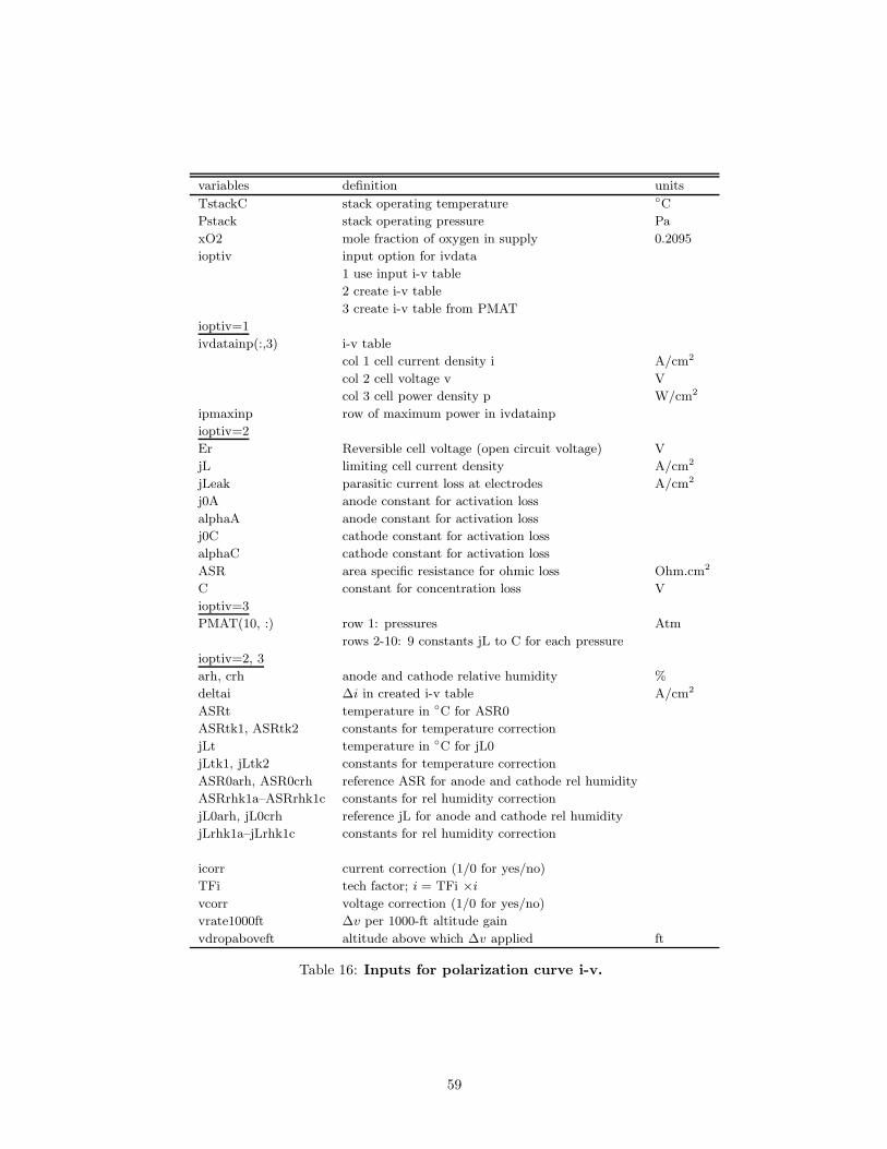
variables definition units
TstackC stack operating temperature C
Pstack stack operating pressure Pa
xO2 mole fraction of oxygen in supply 0.2095
ioptiv input option for ivdata
1 use input i-v table
2 create i-v table
3 create i-v table from PMAT
ioptiv=1
ivdatainp(:,3) i-v table
col 1 cell current density i A/cm2
col 2 cell voltage v V
col 3 cell power density p W/cm2
ipmaxinp row of maximum power in ivdatainp
ioptiv=2
Er Reversible cell voltage (open circuit voltage) V
jL limiting cell current density A/cm2
jLeak parasitic current loss at electrodes A/cm2
j0A anode constant for activation loss
alphaA anode constant for activation loss
j0C cathode constant for activation loss
alphaC cathode constant for activation loss
ASR area specific resistance for ohmic loss Ohm.cm2
C constant for concentration loss V
ioptiv=3
PMAT(10, :) row 1: pressures Atm
rows 2-10: 9 constants jL to C for each pressure
ioptiv=2, 3
arh, crh anode and cathode relative humidity %
deltai ∆i in created i-v table A/cm2
ASRt temperature in C for ASR0
ASRtk1, ASRtk2 constants for temperature correction
jLt temperature in C for jL0
jLtk1, jLtk2 constants for temperature correction
ASR0arh, ASR0crh reference ASR for anode and cathode rel humidity
ASRrhk1a–ASRrhk1c constants for rel humidity correction
jL0arh, jL0crh reference jL for anode and cathode rel humidity
jLrhk1a–jLrhk1c constants for rel humidity correction
icorr current correction (1/0 for yes/no)
TFi tech factor; i = TFi ×i
vcorr voltage correction (1/0 for yes/no)
vrate1000ft ∆v per 1000-ft altitude gain
vdropaboveft altitude above which ∆v applied ft
Table 16: Inputs for polarization curve i-v.
59

variables definition units
ioptsw input option for stack weight
0 simple
1 detailed
TFwstack tech factor, weight
TFsstack tech factor, volume
dWwstack correction weight kg
dSsstack correction volume m3
ioptsw=0
tcell thickness of a cell m
dcell density of stack kg/m3
porosity porosity of stack fraction
ioptsw=1
dendplate density of end-plate (2 per stack) kg/m3
dinsulplate density of insulator plate (2 per stack) kg/m3
dcollplate density of current collector (2 per stack) kg/m3
dpem density of proton exchange membrane kg/m3
dgdl density of gas diffusion layer (2 per pem) kg/m3
dbipolarplate density of bipolar plate electrodes (2 per pem) kg/m3
dgasket density of sealing gasket (2 per pem) kg/m3
Aendplatefrac area of end plate fraction active area
tendplatecons thickness of end plate, constant m
tendplatefrac thickness of end plate, fraction thickness of unit
Ainsulplate area of insulating plate, fraction active area
tinsulplatecons thickness of insulating plate, constant m
tinsulplatefrac thickness of insulating plate, fraction thickness of unit
Acollplatefrac area of collector plate, fraction active area
tcollplatecons thickness of collector plate, constant m
tcollplatefrac thickness of collector plate, fraction thickness of unit
Wfastener weight of fastener kg
tpem thickness of pem m
tgdl thickness of gas diffusion layer m
tbipolarplate thickness of bipolarplate m
pbipolarplate porosity of bipolarplate
Abipolarplatefrac area of bipolarplate, fraction active area
tgasket thickness of gasket m
Agasketfrac area of gasket, fraction active area
Wstackother other weights kg
Table 17: Inputs for stack weight.
60

variables definition units
fH2utilization H2 utilization factor (≈ 1 − 1.05)
h2tankwfg wt fraction gravimetric kg/kg
= h2 weight ÷ (h2+tank) weight
itanktype type of tank volume model
1 input wt fraction volumetric
2 liquid hydrogen
3 compressed gas
itanktype=1
h2tankwfs weight fraction volumetric ρh2 store kg/m3
= h2 weight ÷ tank volume (storage density)
itanktype=2, 3
h2tankSov tank volume overhead sov
= (vol tank - vol h2) ÷ vol tank
itanktype=3
h2tankTC compressed gas temperature C
h2tankBar compressed gas pressure bar
ioptf fuel option for energy calculation
1 input weight of hydrogen
2 input time
ioptf=1
Whydrogen weight of hydrogen kg
ioptf=2
Endurance min duration of design power min
FGErho base fuel density kg/m3
FGEMJkg base fuel ∆h MJ/kg
FGEeta base fuel engine efficiency
P0 power, prescribed W
k, e power, constant and exponent
W0 wt, prescribed, for filter, regulator, power kg
fW wt, fraction system weight
Table 18: Inputs for hydrogen system. The base fuel inputs are used only for gallon equivalents.
61

variables definition units
fAirFlowRate air utilization factor (≈ 2.5)
DPstack Stack pressure drop Pa
iBlower 1/0 for yes/no
iCompressor 1/0 for yes/no
iTurbine 1/0 for yes/no; turned 0 for iCompressor=0
blower, compressor, and turbine
Eta Efficiency
W0 wt, prescribed kg
Wtf wt, technology factor
Wk, Wfe, Wpe wt, constant and flow and power exponents
S0 vol, prescribed m3
Stf vol, technology factor
Sk, Sfe, Spe vol, constant and flow and power exponents
filter, regulator, power, humidifier
W0 wt, prescribed kg
fW wt, fraction system weight
PlumbW0 wt, prescribed
PlumbWl length of plumbing m
PlumbWw weight per length kg/m
Table 19: Inputs for air-supply system.
62

variables definition units
iHV Heating values used for sizing
0-LHV, 1-HHV
iHTR Power level used in sizing
0-design power, 1-max power
coolantCp Cp of coolant fluid J/kg-K
coolantdT Coolant rise in temperature K
W0coolant wt, constant, coolant kg
W0k wt, constant of flow sec
radiator
W0 wt, prescribed kg
Wk, We, Wf wt, constant, heat, and area exponents
Wk = 0 zero area
Wf = 0 unknown area
Wf = 1, We = 0, calculated area, Wk = kg/m2
S0 vol, prescribed m3
Sk, Se, Sf vol, constant, heat, and area exponents
Sk = 0 zero area
Sf = 0 unknown area
Sf = 1, We = 0, calculated area, Sk = thickness in m
radiator area
h radiator heat transfer coefficient W/m2/K
Tr radiator temperature K
Ta ambient temperature for cooling K
epr radiator emissivity
stack dissipation
fd fraction of stack heat
hs stack heat transfer coefficient W/m2/K
Tas ambient temperature for cooling K
eps stack emissivity
fs stack surface area, fraction active area
filter, regulator, power
W0 wt, prescribed kg
fW wt, fraction system weight
PlumbW0 wt, prescribed
PlumbWl length of plumbing m
PlumbWw weight per length kg/m
P0 power, prescribed W
k, e, f power, constant, heat and coolant flow exponent
Table 20: Inputs for the high temperature cooling system.
63

variables definition units
iLTR Power level used in sizing
0-design power, 1-max power
coolantCp Cp of coolant fluid J/kg-K
coolantdT Coolant ambient temperature K
W0coolant wt, constant, coolant kg
W0k wt, constant of flow sec
radiator
W0 wt, prescribed kg
Wk, We, Wf wt, constant, heat, and area exponents
Wk = 0 zero area
Wf = 0 unknown area
Wf = 1, We = 0, calculated area, Wk = kg/m2
S0 vol, prescribed m3
Sk, Se, Sf vol, constant, heat, and area exponents
Sk = 0 zero area
Sf = 0 unknown area
Sf = 1, We = 0, calculated area, Sk = thickness in m
radiator area
h radiator heat transfer coefficient W/m2/K
Tr radiator temperature K
Ta ambient temperature for cooling K
eps radiator emissivity
cooler
W0 wt, prescribed kg
Wk, We wt, constant and heat exponents
filter, regulator, power
W0 wt, prescribed kg
fW wt, fraction system weight
PlumbW0 wt, prescribed
PlumbWl length of plumbing m
PlumbWw weight per length kg/m
P0 power, prescribed W
k, e, f power, constant, heat and coolant flow exponent
Table 21: Inputs for the low temperature cooling system.
64

variables definition units
rhowater density of water kg/m3
waterstoragefrac frac of produced water stored
waterstoragehour for how long hr
watertankSov tank volume overhead
watertankWov tank weight overhead
filter, regulator, power
W0 wt, prescribed kg
fW wt, fraction system weight
PlumbW0 wt, prescribed
PlumbWl length of plumbing m
PlumbWw weight per length kg/m
P0 power, prescribed W
k, e power, constant and exponent
Table 22: Inputs for water storage system.
variables definition units
controller
W0 wt, prescribed kg
Wk, We wt, constant and current exponent
regulator, power
W0 wt, prescribed kg
fW wt, fraction system weight
PlumbW0 wt, prescribed
PlumbWl length of wiring m
PlumbWwk weight per length constant
PlumbWwe weight per length current exponent
P0 power, prescribed W
k, e power, constant and exponent
Table 23: Inputs for electrical systems.
variables definition units
unforeseen overheads
fovpower power, fraction total power
fovweight weight, fraction total weight
fovvolume volume, fraction total volume
iplotVIP plot stack i-v-p 1/0 yes/no
iprntSCR screen output 1/0 yes/no
Table 24: Other inputs.
65

The outputs of design are shown in Table 25. All variables are within the data structure FCST. For exam-ple the variable ivdata is really FCST.ivdata. The design outputs are produced by the driver driverpemfc.m
and driverpemfcdesign.m.The outputs of analysis have the same variable names and are not repeated. But they are fewer in
number as the stack is already designed. They are within the data structure FCOP. The analysis outputsare produced by the driver pemfcstatic.m. Analysis should be performed only after design. See Examples inlater sections.
variables definition units
Cell/stack performance
ivdata(:,3) cell i − v − p table usedcol 1: i, current density A/cm2
col 2: v, voltage Vcol 3: p, power density W/cm2
Eh Eh, ideal reversible cell voltage (enthalpy) VEr Er, true reversible cell voltage (Gibbs) VAactive cm2 Ac, cell active area cm2
Ncell nc, number of cellsIstackdsg stack current at design power AVstackdsg stack voltage at design power VIstackmax stack current max AVstackmax stack voltage max VIstackPmax stack current at max power AVstackPmax stack voltage at max power Vvcdsg vc, cell voltage, design Vicdsg ic, cell current density, design A/m2
pcdsg pc, cell power density, design W/m2
etadsgHHV η, true efficiency, design power with HHV Eh
etadsgLHV η, true efficiency, design power with LHV Eh
etamaxHHV η, true efficiency, max power with HHV Eh
etamaxLHV η, true efficiency, max power with LHV Eh
etavdsgHHV ηr, voltage efficiency, design power with HHV Er
etavdsgLHV ηr, voltage efficiency, design power with LHV Er
Cell/stack size
Sstack stack volume m3
Lstack stack length mAstack stack cross-sectional area m2
Wstack stack weight data structure.total weight, total kg
total = end + insulating + collector + unit.endplate weight, end plate kg.insulplate weight, insulating plate kg.collplate weight, collector plate kg.unit weight, unit kg
unit = number of cells × weight of each cell.cell weight, cell kg
cell = mea + bipolar plates.bipolarplate weight, bipolar plates kg
Continued on next page
66

Table 25 – Continued from previous page
variables definition units
.mea weight, membrane electrode assembly kgmea = pem + gdl + gasket
.pem weight, membrane kg
.gdl weight, gas diffusion layers kg
.gasket weight, gaskets kg
.other weight, other kgWstackk0 k0, design factor constant kgWstackk1 k1, design factor constant kg/m2
DFstack design factor, pc/( P/Wstack ) kg/m2
SP specific power, design power kW/kgSPmax specific power, max power kW/kg
Air systemSblower volume, blower m3
Scomp volume, compressor m3
Sturb volume, turbine m3
Pblower kW power, blower, design kWPblowermax kW power, blower, max kWPcomp kW power, compressor, design kWPcompmax kW power, compressor, max kWPturb kW power, turbine, design kWPturbmax kW power, turbine, max kWPair kW power, total, design kWPairmax kW power, total, max kWWair weight kg.total total kg.blower blower kg.comp compressor kg.turb turbine kg.precooler precooler kg.humidifier humidifier kg.filter filter kg.plumbing plumbing kg.power power components kg.regulator regulators kgMassAirrate kgs air mass flow, design power kg/sMassAirrate max kgs air mass flow, max power kg/sMassAirrate Ls air volume flow, design power L/sMassAirrate max Ls air volume flow, max power L/sMassAirrate out kgs air mass flow out, design power kg/sMassAirrate out max kgs air mass flow out, max power kg/sHumidity ratio humidity ratio out, design powerMassWaterrate kgs water mass flow out, design power kg/sMassVaporrate kgs water vapor mass flow out, design power kg/sMassLiquidrate kgs water liquid mass flow out, design power kg/s
Continued on next page
67

Table 25 – Continued from previous page
variables definition units
Fuel/H2 system
Sh2tank volume of H2 tank m3
Wfuel weight of H2 fuel system kg.total weight, total kg.H2 weight, H2 kg.tank weight, tank kg.filter weight, filters kg.plumbing weight, plumbing kg.power weight, power components kg.regulator weight, regulators kgPfuel kW power, fuel system, design power kWPfuelmax kW power, fuel system, max power kWMassH2rate kgs H2 mass flow, design power kg/sMassH2rate Pmax kgs H2 mass flow, max power kg/sSFCPdsg kgkWh SFC, design power kg/kW-hrSFCPmax kgkWh SFC, max power kg/kW-hr
Low temp cooling (ltc)
Wlt weight of ltc system kg.total weight, total kg.filter weight, filters kg.plumbing weight, plumbing kg.regulator weight, regulators kg.coolant weight, coolant liquid kg.radiator weight, radiator kg.power weight, power components kgPlt kW power, ltc, design power kWPltmax kW power, ltc, max power kWSltradiator volume, radiator m3
Altradiator area, radiator m2
HEATINGlt kW heat load kWHEATINGlt max kW heat load max kWCflowdsglt coolant flow, design power kg/sCflowmaxlt coolant flow, max power kg/sCflowlt coolant flow used for ltc sizing kg/s
= Cflowdsglt for input iLTR=0
High temp cooling (htc)
Wht weight of htc system kg.total weight, total kg.filter weight, filters kg.plumbing weight, plumbing kg.regulator weight, regulators kg.coolant weight, coolant liquid kg.radiator weight, radiator kg.power weight, power components kg
Continued on next page
68
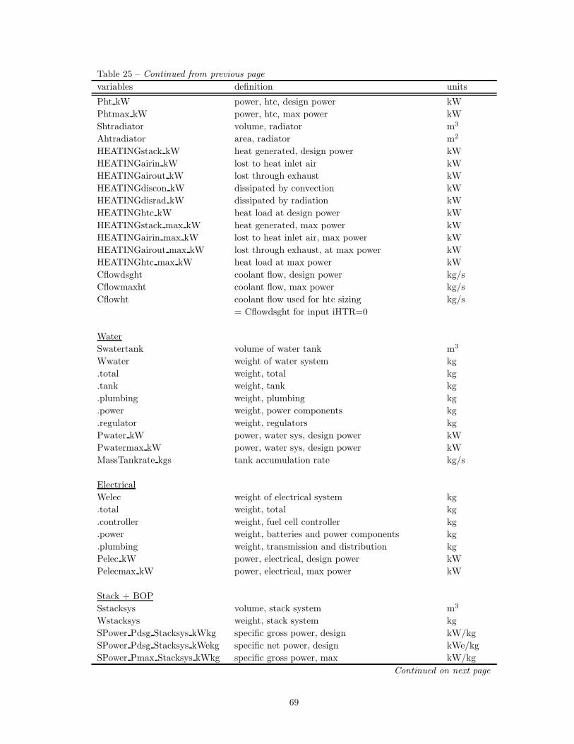
Table 25 – Continued from previous page
variables definition units
Pht kW power, htc, design power kWPhtmax kW power, htc, max power kWShtradiator volume, radiator m3
Ahtradiator area, radiator m2
HEATINGstack kW heat generated, design power kWHEATINGairin kW lost to heat inlet air kWHEATINGairout kW lost through exhaust kWHEATINGdiscon kW dissipated by convection kWHEATINGdisrad kW dissipated by radiation kWHEATINGhtc kW heat load at design power kWHEATINGstack max kW heat generated, max power kWHEATINGairin max kW lost to heat inlet air, max power kWHEATINGairout max kW lost through exhaust, at max power kWHEATINGhtc max kW heat load at max power kWCflowdsght coolant flow, design power kg/sCflowmaxht coolant flow, max power kg/sCflowht coolant flow used for htc sizing kg/s
= Cflowdsght for input iHTR=0
WaterSwatertank volume of water tank m3
Wwater weight of water system kg.total weight, total kg.tank weight, tank kg.plumbing weight, plumbing kg.power weight, power components kg.regulator weight, regulators kgPwater kW power, water sys, design power kWPwatermax kW power, water sys, design power kWMassTankrate kgs tank accumulation rate kg/s
ElectricalWelec weight of electrical system kg.total weight, total kg.controller weight, fuel cell controller kg.power weight, batteries and power components kg.plumbing weight, transmission and distribution kgPelec kW power, electrical, design power kWPelecmax kW power, electrical, max power kW
Stack + BOPSstacksys volume, stack system m3
Wstacksys weight, stack system kgSPower Pdsg Stacksys kWkg specific gross power, design kW/kgSPower Pdsg Stacksys kWekg specific net power, design kWe/kgSPower Pmax Stacksys kWkg specific gross power, max kW/kg
Continued on next page
69

Table 25 – Continued from previous page
variables definition units
SPower Pmax Stacksys kWekg specific net power, max kWe/kgDFstacksys design factor, pc/( P/Wstacksys ) kg/m2
Total SystemStotal volume, total system m3
Wtotal weight, total system kgPOWERdsg kWe net electrical design power kWePOWERmax kW gross max power kWPOWERmax kWe net electrical max power kWeEtadsgHHV true efficiency at design power using HHVEtadsgLHV true efficiency at design power using LHVEtamaxHHV true efficiency at max power using HHVEtamaxLHV true efficiency at max power using LHVFGEHHV Fuel gallon equivalent using HHV (chemical) galFGELHV Fuel gallon equivalent using HHV (chemical) galFGEHHVtrue chemical × efficiency galFGELHVtrue chemical × efficiency galSFCPdsg kgkWhe SFC, at net electrical design power kg/kWe-hrSFCPmax kgkWhe SFC, at net electrical max power kg/kWe-hrENERGY Pdsg kWh energy capacity, at design power kWhENERGY Pdsg kWhe net electrical energy at design power kWe-hrENERGY Pmax kWhe net electrical energy at max power kWe-hrENERGY Pmax kWh gross energy capacity at max power kW-hrSPower Pdsg kWkg specific gross power kW/kgSPower Pdsg kWekg specific net power kWe/kgSPower Pmax kWkg specific gross max power kW/kgSPower Pmax kWekg specific net max power kWe/kgEDensity Pdsg kWhL energy density at gross design power kW-hr/LEDensity Pdsg kWheL energy density at net design power kWe-hr/LEDensity Pmax kWhL energy density at gross max power kW-hr/LEDensity Pmax kWheL energy density at net max power kWe-hr/LSEnergy Pdsg kWhkg specific energy at gross design power kW-hr/kgSEnergy Pdsg kWhekg specific energy at net design power kWe-hr/kgSEnergy Pmax kWhkg specific energy at gross max power kW-hr/kgSEnergy Pmax kWhekg specific energy at net max power kWe-hr/kg
Table 25: Outputs of stack design. All variables are within the datastructure FCST. Design and max power refer to conditions whenstack generates design and maximum power. L=Liter. gal=U.S.gallon. HHV=Higher Heating Value of H2. LHV=Lower HeatingValue of H2.
70

The variables required to design the rotorcraft are acquired by executing the driverpemfc.m and pemfc-
static.m over a range of inputs. These variables and corresponding drivers are listed in Table 26. The driverinputs over write fcvariables.m.
variables definition units
driverpemfcPvsW.m
FCST.
StackWvsP(:,2) gross power, stack weight kW, kg
StackSystemWvsPe(:,3) net power, net power max, stack sys weight kWe, kWe, kg
stack sys = total system - fuel - tank
driverpemfcWvsH.m
FCST.
StackSystemWvsH(:,2) altitude, stack sys weight m, kg
driverpemfcenginechartvsH.m
FCOP.
Pevs1000ft(:,5) col 1: altitude 1000-ft
col 2, 3: power, net power kW, kWe
col 4, 5: SFC, fuel flow kg/kW-hr, kg/hr
driverpemfcenginechartvsP.m
FCOP.
H2flowvsP(:,2) net power, fuel flow kWe, kg/hr
SFCvsP(:,2) net power, SFC kWe, kg/kW-hr
SFCvsPefrac(:,2) power fraction, SFC non-dim, kg/kW-hr
power fraction = net power ÷ net design power
Table 26: Drivers and outputs for rotorcraft design.
71

11 Example: Baseline 80 kW
A hypothetical PEMFC system of net power 80 kWe (kW-electrical) is sized with cell characteristics givenin Figs 11 and 12 (data from Yan, Toghiani and Wu 2006). These are representative of Yr-2000 technologyand considered the baseline.
The model constants for i − v curves for pressures 1 to 4 atm were given in Table 8. Temperature andhumidity corrections were extracted for area specific resistance and the limiting current about the referencetemperature 80C (353.15 K) and reference humidity 100%. In absence of data, the same corrections wereassumed to apply to all pressures. The symbols have usual meanings and units (see Section on Theory/Thei − v Curve).
The temperature corrections are the following.
∆ASRΩ = 0.002 (T − 353.15) + 0.0006 (T − 353.15)2
∆iL = −0.003 (T − 353.15)− 0.0015 (T − 353.15)2
The humidity corrections are the following.
a = arh − 100
c = arh − 100
∆ASRΩ = −0.005a + 2 × 10⁻⁶ a c2 + 7 × 10⁻⁵ c2 + 0.0021 c
∆iL = −1 × 10⁻⁴ c2 − 0.0076 c
The example case is given in the run directory run Baseline 80kW.The stack pressure is specified as 2.5 atm. So the 2 and 3 atm model constants in Table 8 are interpolated
linearly for cell i − v. The stack temperature is specified as 80C which is the temperature of the dataset.The driver drivercreateiv.m is used to calculate the model constants. The i−v data is available for 1, 2, 3,
and 4 atm pressures. The constants in Table 8 produced good fits.Figure 21 shows the voltage data at 2 and 3 atm and the model fit for 2.5 atm. The cell power density
is p = i v, and the heat density is q = i (Eh − v). The true efficiency and the voltage efficiency (Eq 16)are shown in Fig 22. There is nominally no maximum efficiency point, the peak is merely an artifact of theleakage current. Higher efficiencies are obtained at lower currents (lower power) and lower efficiencies athigher currents (higher power). So the maximum power density generally occurs at low efficiency.
The driver drivercreateiv.m outputs an i−v−p data table and a variable ipmax which is the row numberof maximum power. The resolution ∆i is set by the variable deltai (deltai = 0.01 is used). The i − v − ptable and ipmax are input in fcvariables.m as ivdatainp and ipmaxinp.
The model fit is input in fcvariables.m. For option ioptiv=1, the data table i−v−p is input as ivdatainpalong with the row number of maximum power ipmaxinp; for ioptiv=2, the 9 constants are input; and forioptiv=3, a matrix PMAT is input which contains the 9 constants for each pressure.
There can be a loss in cell voltage from cell-level to the stack-level. The variable deltav accounts for thisloss. A typical value for a 80 kWe stack is 0.01 V. There can be a drop in cell voltage with altitude when acompressor is not used. A typical value is 0.56% per 1000-ft. A base altitude can be input above which thecorrection is applied. The variable vcorr determines whether these corrections are applied. Here vcorr=0 sono corrections are applied.
vcorr = 0
72

0 0.2 0.4 0.6 0.8 1 1.2 1.40
0.2
0.4
0.6
0.8
1
1.2
1.4
1.6
Current density, A/cm2
Cel
l vol
tage
, V; P
ower
den
sity
, W/c
m2 ; Hea
t, W
/cm
2
Data3 atm
voltage
Er = 1.1782 V
Eh = 1.4722 V
Data2 atm
power
heat
Figure 21: Cell voltage, power, and heating versus current of baseline cells representative ofYr-2000 technology. Symbols are data at 2 and 3 atm. Lines are models at 2.5 atm. 80C.100% anode and cathode relative humidity.
0 0.2 0.4 0.6 0.8 1 1.2 1.40
0.1
0.2
0.3
0.4
0.5
0.6
0.7
Current density, A/cm2
Cel
l effi
cien
cy
True efficiencyVoltage efficiency
Figure 22: Cell efficiency of baseline cells at 2.5 atm, 80C.
73

deltav = -0.01vrate1000ft = -0.0056vdropaboveft = 1000The stack is built of conventional materials.The end plate is Aluminum (ρ = 1600 kg/m3), the insulation plate is polyoxy-methylene (ρ = 1420
kg/m3), the collector plate is Copper (ρ = 8940 kg/m3), the membrane is Nafion (ρ = 500 kg/m3), the gasdiffusion layer and catalyst layer are a single carbon cloth coated with Pt/C on one side (ρ = 440 kg/m3),the bipolarplate is graphite (ρ = 2160 kg/m3), and the gasket is rubber (ρ = 1000 kg/m3). These inputscan be changed based on an actual stack.
A technology factor can be specified.TFwstack = 1.0The design environment is SL/ISA. This impacts the balance of plant.The driver driverpemfc.m sizes a stack for a gross power given by the input POWERdsg kW. The net
electric power is lower due to the balance of plant. The option ioptp=1 produces a stack of minimum weight.For this option, the cell operates at the maximum power density, hence at a low voltage (Fig 21), andtherefore at a poor efficiency (Fig 22) (efficiency is ≈ v/1.4722). The option ioptp=3, with voltage specifiedas vc=0.6, produces a stack of high efficiency. For this option, the maximum power is higher than the designpower.
The cooling systems can be sized either to design power or to maximum power. In this example, it issized to the design power.
iLTR = 0iHTR = 0The high temperature cooling system is the stack cooling system. The heat load can be specified either
for LHV (product water in vapor form, Eh = 1.256 V) or HHV (product water in liquid form, Eh = 1.4722V). Less cooling is needed when the water is in vapor form as the heat of vaporization is not released. Inthis example, the LHV is used.
iHV = 0Hydrogen is stored at 5.7% weight fraction as compressed gas at 700 bar 15C. For option ioptf=1, the
amount of hydrogen is specified. In this example 5 kg is assumed.H2wfrac = 0.057Whydrogen = 5h2tankBar = 700h2tankTC = 15Table 27 shows two stack designs — minimum weight and high efficiency (based on input voltage vc
selected from Fig 22). In the table, only the variables that change from one column to the next are shown,an empty column means a repeated value. The outputs are saved in files B80minwgtDESIGN.tex andB80highetaDESIGN.tex.
In the minimum weight design, the design power 80 kWe is the maximum power and the maximumcontinuous power (MCP). In the high efficiency design, the design power 80 kWe is the maximum continouspower (MCP), but it is not the maximum power. The maximum power is 95 kWe. But since the stackcooling system is sized to the design power, this is not continuous power. 95 kWe is 1.188 × 80 kWe which isclose to the typical intermediate rated power factor for helicopters (IRP=1.185) but short of the maximumrated power factor (MRP=1.269) and the contingency rated power factor (CRP=1.33). These margins canbe provided if the stack is sized to higher efficiencies (by increasing input voltage vc) but at the cost of higherweight.
In summary, baseline cells can provide typical power densities pc ≈ 0.30 − 0.37 W/cm2 at efficiencies ofη ≈ 0.3 − 0.4. Specific power of the stack can be 0.8 − 1.0 kW/kg with a charitable design factor of 3.5kg/m2. But specific power of the stack system is what is more important. This is driven by the weight of the
74

Component Variables Unit B80 B80
min weight high η
Cell vc V 0.458 0.601
pc W/cm2 0.375 0.303
ηc, ηv 0.31, 0.38, 0.40, 0.50
Weight kg 0.15 0.23
Stack No of cells 546 416
Active area cm2 470 731
Weight kg 90 107
Sp power kW/kg 1.07 0.86
Design fac kg/m2 3.52
Air Air flow kg/s 0.19 0.14
Power kW 12.7 9.3
Weight kg 17.5 20.8
HT cool Q gen kW 170 102
Q load kW 153 87
Q/∆T kW/C 2.3 1.3
Power kW 1.5 0.87
Weight kg 1.7 0.99
LT cool Q gen kW 9.6 6.9
Power kW 0.10 0.07
Weight kg 1.0 0.74
Electrical Power kW 1.9 1.8
Weight kg 4.8 7.5
Stack system
P, P net kW, kWe 96, 80
Pmax, Pmax net kW, kWe 96, 80 114, 95
Weight kg 116 137
Sp Power kWe/kg 0.69 0.58
Fuel H2 flow kg/s 0.0022 0.0016
H2 stored kg 5
Tank wt% 5.7
Total Weight kg 90
Total system
Endurance min 38 51
Energy kWhe 50 68
Weight kg 205 227
Sp Power kWe/kg 0.39 0.35
Sp Energy kWe-hr/kg 0.24 0.30
Energy density kWe/L 0.21 0.29
η 0.26 0.35
GGE U.S. gal 5.5 4.0
Table 27: 80 kWe PEMFC designs with baseline cells. SL/ISA. Stack: 250V, 2.5 atm, 80C;tank: 700 bar, 15C; cell: Eh, Er: 1.47, 1.18 V (HHV) and 1.26, 1.17 (LHV). No water tank.ηc, ηv: true (HHV) and voltage efficiencies of cell; η: efficiency of the system (HHV). Gallongasoline equivalent (GGE) based on combustion efficiency 0.25.
75

balance of plant subsystems, particularly the air and the cooling systems. The stack system specific poweris placed around 0.6 − 0.7 kWe/kg in this example.
Comparison with batteries must include the hydrogen and tank weight. In this example, with 5 kghydrogen storage, the specific energy and power are around 240 − 300 Wh/kg and 0.39 − 0.35 kW/kgrespectively, where the net electrical energy and power are used. The specific power is equivalent to batteryC-rates of 1.625 —1.167 (390 W/240 Wh — 350 W/300 Wh), where the lower C-rate corresponds to thehigher specific energy — a behavior consistent with any electrochemical source. Note that the batteryspecifications used for comparison should be pack level, available and installed.
76

12 Example: Modern 80 kW
A hypothetical PEMFC system of net power 80 kWe (kW-electrical) is sized with cell characteristics givenin Figs 13 and 14 (Alhuwalia, Wang and Steinbach 2016). These are representative of modern automobilefuel cells. This example can be used as a template for a DOE HP benchmark stack.
Only the cell characteristics are changed from the previous example, so the new results reflect only theimpact of advanced electrochemistry.
The model constants for the relevant i − v curves were given in Table 9. In absence of data, the samecorrections are retained for temperature and humidity as the baseline cells.
The example cases are given in the run directories run Modern 80kW and run Modern 80kW liqcool. Theliqcool example has additional inputs to size radiators and coolants.
The stack pressure is again specified as 2.5 atm. The model constants need not be interpolated sincedata is available at this pressure. The stack temperature is again 80C.
The driver drivercreateiv.m is used to calculate the model constants. The i − v data is available for1, 1.25, 1.5, 2.0 and 2.5 atm. The constants in Table 9 produced good fits.
Figure 23 shows the data and the model fit. The true efficiency and the voltage efficiency of the cell(Eq 16) are shown in Fig 24. There is truly no maximum efficiency point, the peak efficiency is merelyan artifact of the leakage current. The leakage current is quite high in this example, hence the waveformdifferent from the baseline cell, with a clear maximum around vc ≈ 0.7 V.
The driver drivercreateiv.m outputs an i−v−p data table and a variable ipmax which is the row numberof maximum power. The resolution ∆i is set by the variable deltai (deltai = 0.01 is used). The i − v − ptable and ipmax are input in fcvariables.m as ivdatainp and ipmaxinp.
The model fit is input in fcvariables.m. For option ioptiv=1, the data table i−v−p is input as ivdatainpalong with the row number of maximum power ipmaxinp; for ioptiv=2, the 9 constants are input; and forioptiv=3, a matrix PMAT is input which contains the 9 constants for each pressure.
The stack is built of same materials as the baseline stack.The design environment remains SL/ISA.The driver driverpemfc.m sizes a stack for a gross power given by the input POWERdsg kW. The net
electric power is lower due to balance of plant. The option ioptp=1 produces a stack of minimum weight. Forthis option, the cell at maximum power density hence a low voltage (Fig 23) and therefore a low efficiency(Fig 24) (efficiency is ≈ v/1.4722). The option ioptp=3, with voltage specified as vc=0.7, produces a stacknear maximum efficiency. For this option, the maximum power is also higher than the design power.
The cooling systems are still sized to the design power as the baseline case.The heat load is specified for LHV as the baseline case.Hydrogen is stored at 5.7% weight fraction as compressed gas at 700 bar 15C. For option ioptf=1, the
amount of hydrogen is specified. In this example 5 kg is assumed.H2wfrac = 0.057Whydrogen = 5h2tankBar = 700h2tankTC = 15Table 28 shows two stack designs (columns 4 and 5) — minimum weight and high efficiency (as determined
by the input cell voltage). In the table, only the variables that change from one column to the next areshown, an empty column is a repeat value. The outputs are saved in files M80minwgtDESIGN.tex andM80highetaDESIGN.tex.
77

0 0.2 0.4 0.6 0.8 1 1.2 1.4 1.6 1.8 20
0.2
0.4
0.6
0.8
1
1.2
Current density, A/cm2
Cel
l vol
tage
, V; P
ower
den
sity
, W/c
m2
Cell voltage, VCell power density, W/cm2
Data
Model POWER
VOLTAGE
Figure 23: Cell voltage, power, and heating versus current of modern automobile cells repre-sentative of Yr-2020 technology. Symbols are data at 2.5atm. Lines are models. 80C.
0 0.2 0.4 0.6 0.8 1 1.2 1.4 1.6 1.8 20
0.1
0.2
0.3
0.4
0.5
Current density, A/cm2
Cel
l effi
cien
cy
True efficiencyVoltage efficiency
Figure 24: Cell efficiency of modern cells at 2.5 atm, 80C.
78

Component Variables Unit M80 M80 M80
min weight max η max η/liq cool
Cell vc V 0.564 0.700
pc W/cm2 1.116 0.734
ηc, ηv 0.33, 0.42, 0.37, 0.46
Weight kg 0.06 0.11
Stack No of cells 443 357
Active area cm2 192 355
Weight kg 30 45
Sp power kW/kg 3.2 2.1
Design fac kg/m2 3.52
Air Air flow kg/s 0.1732 0.1529
Power kW 11.6 10.2
Weight kg 16 24
HT cool Q gen kW 134 95
Q load kW 122 83
Q/∆T kW/C 1.9 1.3
Power kW 1.2 0.82 0.59
Weight kg 1.4 0.9 44
LT cool Q gen kW 8.7 7.7 13
Power kW 0.09 0.08 0.06
Weight kg 0.9 0.8 6.9
Electrical Power kW 1.9 1.9
Weight kg 4.1 7.7
Stack system
P, P net kW, kWe 95, 80 93, 80
Pmax, Pmax net kW, kWe 95, 80 141, 119
Weight kg 52 78 127
Sp Power kWe/kg 1.53 1.03 0.63
Fuel H2 flow kg/s 0.002 0.0018
H2 stored kg 5
Tank wt% 5.7
Tank + H2 kg 90
Total system
Endurance min 41 47
Energy kWhe 55 62
Weight kg 142 167 216
Sp Power kWe/kg 0.56 0.48 0.37
Sp Energy kWe-hr/kg 0.39 0.37 0.29
Energy density kWe/L 0.3 0.32 0.28
η 0.28 0.32
GGE U.S. gal 5.0 4.4
Table 28: 80 kWe PEMFC designs with modern cells. SL/ISA. Stack: 250V, 2.5 atm, 80C;tank: 700 bar, 15C; cell: Eh, Er: 1.47, 1.18 V (HHV) and 1.26, 1.17 (LHV). No water tank.ηc, ηv: true (HHV) and voltage efficiencies of cell; η: efficiency of the system (HHV). Gasolinegallon equivalent (GGE) based on combustion efficiency 0.25. Liquid cooling is sized to designpower.
79

The high efficiency design mimics the Toyota Mirai loosely, based on the few details that are easilyavailable: cell weight 0.102 kg, number of cells 370, maximum power output 114 kW (kW or kWe unclear),5 kg hydrogen storage at 700 bar, tank wt% 5.7, and tank internal volume of 122.4 L. The example assumesa storage temperature of 15C and predicts 126 L.
In the minimum weight design, the design power 80 kWe is the maximum power and the maximumcontinuous power (MCP). In the high efficiency design, the design power 80 kWe is the maximum continouspower (MCP), but it is not the maximum power. The maximum power is 119 kWe. But since the stackcooling system is sized to the design power, this is not continuous power. 119 kWe is 1.475 × 80 kWe whichis ample margin to cover all rated power factors — intermediate rated power factor (IRP=1.185), maximumrated power factor (MRP=1.269) and contingency rated power factor (CRP=1.33). These margins can bereduced if the stack is sized to lower efficiencies (input voltage vc) which would also reduce its weight.
In summary, modern cells can provide typical power densities pc ≈ 0.7 − 1.1 W/cm2 at efficiencies ofη ≈ 0.33−0.37. These power densities are twice as high as the baseline cells. Specific power of the stack canbe 2− 3 kW/kg with a charitable design factor of 3.5 kg/m2. Note that the stack design factor remains thesame as baseline cells since no change is made to the structure and materials. But specific power of the stacksystem is what is more important. This value is driven by the weight of the balance of plant componentsparticularly air and heat. The stack system specific power is placed around 1.0 − 1.5 kWe/kg.
Comparison with batteries must include the hydrogen and tank weight. With modern cells, the specificenergy and power are increased to 370 − 390 Wh/kg and 0.56 − 0.48 kW/kg respectively, where the netelectrical energy and power are used. The specific power is equivalent to battery C-rates of 1.5 — 1.23continuous, where the lower C-rate corresponds to the higher specific energy — a behavior consistent withany electrochemical source. Note that the battery specifications used for comparison should be pack level,available and installed.
For sizing an aircraft, the following power and fuel flow models are required.
1. Weight versus power (design),
2. Weight versus altitude for a specified power (design),
3. Power versus altitude for a specified engine (analysis),
4. Fuel flow versus power for a specified engine (design and analysis), and
5. Power versus velocity for a specified engine (design and analysis).
There is no model for 5. Power versus velocity. Some variation is expected from the airspeed effect oncooling and perhaps even ram effect on the stack pressure and air density. But there is no measured data tobuild such a model.
The following energy and electrical models are needed.
1. Ragone plot of specific power versus specific energy (design), and
2. Current, voltage and power range for a specified engine (analysis).
The drivers that generate these models are now briefly described.The driver driverpemfcPvsW.m generates power versus weight. Figure 25 shows the net electrical power
output versus the weight of the stack system.The driver driverpemfcWvsH.m calculates the stack system weight versus altitude for a specified net
electrical power. Figure 26 shows the variations for two stack designs. The compressor power increases withaltitude which requires a heavier compressor (so the stack system weight is increased), while at the sametime a larger stack is needed to compensate for this loss (so the stack weight is also increased).
The driver driverpemfcragone.m calculates the Ragone plots. Figure 27 shows the Ragone plots for thetwo designs. A Ragone plot shows the variation of specific power and specific energy for the total system
80

between the two extremes of all stack-no fuel and no stack-all fuel. The left end of the plot approaches allstack-no fuel, so the specific energy approaches zero and specific power to that of the stack system alone(Fig 25). The right end of the plot approaches no stack-all fuel, so the specific energy approaches that of thefuel system alone whereas specific power approaches zero. The variation is a straight line, but curves on alog-log plot which is how it is typically plotted. Since power P is related to energy E through time t, P t = E,or log P = log E − log t. For t = 1 hr, log P = log E; for t = 1/2 hr, log P = log E + log 2; for t = 2 hr,log P = log E − log 2; in general then, for t = 2n hr, log P = log E − n log 2, where n = . . . ,−2,−1, 0, 1, 2 . . .produce parallel lines equi-spaced by log 2. The Ragone plots in Fig 27 show that the high efficiency stacksystem is lighter for continuous operations longer than 2 hours and that their maximum power is higher thanthe minimum weight stacks. Thus, the selection of design is governed by the time of continuous operation,and the requirement for intermittent high power. For continuous operation beyond 2 hr, the high efficiencystack will burn less hydrogen and this effect will more than compensate for the stack weight.
Figure 28 shows the dramatic impact of hydrogen storage weight fraction.Figure 29 shows specific power versus energy density.Figure 30 shows the impact of the type of hydrogen storage on the energy density. There is not much to
be gained by increasing pressure; but lowering the temperature could have a major impact. However, noneof these effects are nearly as dramatic as that of a rising weight fraction, as shown in Fig 28.
Once the stack is sized, its operation is determined by the stack current. The stack power and voltagevariations with current are shown in Fig 31, stack efficiency in Fig 32, and stack specific fuel consumption(SFC) in Fig 33.
The driver driverpemfcenginechartvsH.m generates the engine charts of power versus altitude. Figure 34shows these variations.
The driver driverpemfcenginechartvsP.m generates the engine charts of fuel flow versus power. Figure 36shows the specific fuel consumption. The effect of the leakage current is quite significant, particularly at lowpower operation.
The example run Modern 80kW liqcool is same as the maximum efficiency stack, but with the coolingsystems sized in greater detail. The radiator and the coolant weight are now included in sizing. This stackis shown in column 6 of Table 28.
The low temperature cooling system is sized to maximum power.iLTR = 1The high temperature cooling system is sized to the design power.iHTR = 0So the stack can be operated at maximum power as long as the high temperature cooling system would
allow.The radiator ambient temperature is assumed as 20C which is lower than the typical 40C for automobile
fuel cells. The stack ambient temperature is specified as 40C to allow for temperature rise in its housing.For both the cooling systems, the radiator weight is assumed to be 3.5 kg/m2. The radiator temperature isTr = 95C. The coolant is water with specific heat ratio Cp = 4180 J/kg-K and density ρ = 997 kg/m3. Inan actual stack deionized water/Glycol mixer with other additives would be used and properties specifiedaccordingly. The rise in coolant temperature is input as ∆Tc = 10C (typically the maximum is 15C).Coolant volume flow rates of around 70 L/min are predicted which are consistent with a typical automobilefuel cell. Fresh supply for 20 sec continuous is input, which gives a coolant capacity of 23 L. Conventionalautomobiles typically have ≈ 5 − 18 L coolant capacity. The data for fuel cell automobiles is not available.The increase in overall weight is very significant with the radiator and the coolant.
In summary, a more detailed model of the cooling system increased the stack system weight very sig-nificantly from 78 kg to 128 kg. The specific energy and power for the total system are reduced to 290Wh/kg and 0.37 kW/kg respectively, for net electrical energy and power. The specific power is equivalentto a battery C-rate of 1.28. The leakage current was found to have a significant effect on the low poweroperation.
81

0 50 100 150 200 2500
50
100
150
200
250
Stack system Weight, kg
Net
Pow
er, k
We
Max efficiencyη = 0.32
1.03 kWe/kg
Min weightη = 0.28
1.53 kWe/kg
Figure 25: Stack net electrical power (kWe) versus stack system weight (kg). η is systemefficiency.
0 20 40 60 80 100 1200
2
4
6
8
10
12
14
Alti
tude
, x 1
000
ft
Weight, kg
Minweight
Maxefficiency
Minweight
Stackonly
Stacksystem
Maxefficiency
Figure 26: Stack and stack system weight versus altitude/ISA; net electrical power is 80 kWe.
82

102 103
102
103
Specific energy, Whe/kg
Spec
ific
pow
er, W
e/kg
4 hours
2 hours
1 hour
30 mins15 mins
7.5 mins
Max efficiency stack@ max power
Min weight stack
Max efficiency stack@ design power
Figure 27: Ragone plot. Full system specific power versus specific energy. Design power andmaximum power shown for the maximum efficiency stack. Design power = maximum powerfor the minimum weight stack.
102 103102
103
Specific energy, Whe/kg
Spec
ific
pow
er, W
e/kg
4 hours
2 hours
1 hour
30 mins15 mins
7.5 mins
5.7%baseline
15%30%
7.5%
Figure 28: Ragone plot. Impact of hydrogen storage weight fraction 5.7%–30%. Design powershown for the maximum efficiency stack.
83

102 103
102
103
Energy density, Whe/L
Spec
ific
pow
er, W
e/kg
Max efficiency stack@ max power
Max efficiency stack@ design power
Min weight stack
Figure 29: Specific power versus energy density. 700 bar 15C compressed gas storage. De-sign power and maximum power shown for the maximum efficiency stack. Design power =maximum power for the minimum weight stack.
102 103
102
103
Energy density, Whe/L
Spec
ific
pow
er, W
e/kg
Liq H2800b −50C800b 0C800b 15C700b 15C baseline
Figure 30: Specific power versus energy density. Impact of hydrogen storage type. Designpower shown for the maximum efficiency stack.
84

0 100 200 300 400 500 600 700 8000
50
100
150
200
250
300
350
400
Stack current, A
Stac
k vo
ltage
, V; S
tack
Pow
er, k
W
Min weight
250 V
Max efficiency
Max efficiency
VOLTAGE
POWER93 kW
Min weight95 kW
Figure 31: Operating electrical parameters of 80 kWe stacks.
0 100 200 300 400 500 600 700 8000
0.1
0.2
0.3
0.4
0.5
Stack current, A
Stac
k ef
ficie
ncy
Max efficiency stackDesign point
Min weight stackDesign point
0.33
0.37
Figure 32: Operating efficiency of 80 kWe stacks.
85

0 100 200 300 400 500 600 700 8000
0.01
0.02
0.03
0.04
0.05
0.06
0.07
0.08
0.09
0.1
Stack current, A
SFC
, kg
/ kW−h
r
Max efficiency
Min weight
Figure 33: Operating specific fuel consumption of 80 kWe stacks.
0 2 4 6 8 10 12 1455
60
65
70
75
80
85
Altitude, x 1000 ft
Net
Pow
er,k
We
Min weightSL
Min weight5K−ft / 20C
SL
Max efficiency5K−ft / 20C
Figure 34: Operating altitude versus power for 80 kWe stacks. Impact of SL and 5,000-ft /20C designs. Fuel flow fixed at design power 80 kWe.
86

0 20 40 60 80 100 1200
2
4
6
8
10
12
Net Power, kWe
H2
flow
, kg/
hr
SL5,000−ft10,000−ft
Design pointSL/ISA
w/oleakagecurrent
Figure 35: Operating fuel flow versus power at various altitudes for a ISA/SL design. Impactof leakage current.
0 20 40 60 80 100 1200
0.01
0.02
0.03
0.04
0.05
0.06
0.07
0.08
0.09
0.1
0.11
0.12
0.13
Net Power, kWe
SFC
, kg/
kWe−
hr
SL
Design pointSL/ISA
w/oleakagecurrent
5,000−ft
10,000−ft
Figure 36: Operating fuel flow versus power at various altitudes for a ISA/SL design. Impactof leakage current.
87

13 Example: Modern 500 kW
The 80 kWe liquid cooled example of the previous section is extended to a hypothetical 500 kWe power. Inpreparation of rotorcraft sizing, the environment is changed from SL/ISA to 5000-ft / 20C.
The new environment inputs in fcvariables.m are.iatm = 1altitudeDesign = 1524temperatureC = 20Hydrogen is still stored at 5.7% weight fraction as compressed gas at 700 bar 15 C but the amount of
hydrogen is doubled to 10 kg. For option ioptf=1, the amount of hydrogen is specified.H2wfrac = 0.057Whydrogen = 10h2tankBar = 700h2tankTC = 15A 500 kW system designed for rotorcraft will likely require many changes that will affect scaling with
power. These include the radiator heat transfer coefficients, radiator weight along with support structure,the surface area of the stack after packaging, the type of coolant, and coolant capacity. A realistic explorationof these changes require reliable test data.
eVTOL might allow the elimination of some subsystems. For low altitude flight, a pressurized stack maynot be essential, so the compressor-expander can be deleted, and along with it, the low temperature coolingsystem. Because hydrogen storage is needed for only a short duration (1− 3 hr), high weight fraction tanks(15 − 30% or higher) that allow boil-off, may be practical. These excursions are easily modeled. Some ofthem are illustrated below and their impact studied later in rotorcraft sizing.
The same drivers described earlier are used to design the stacks.The driver driverpemfcdesign.m sizes stacks for net electrical power. Table 29 shows four stacks designed
for 500 kWe. Two of these are 2.5 atm stacks (columns 4 and 5) — minimum weight and high efficiency (asdetermined by the input cell voltage from 2.5 atm i− v data), and the other two are 1 atm stacks (columns6 and 7) — minimum weight and high efficiency (as determined by the input cell voltage from 1 atm i − vdata).
The driver driverpemfcPvsW.m generates power versus weight.The relevant output is FCST.StackSystemWvsPe (Table 26) which contains net power, maximum net
power, and the stack system weight. Figure 37 shows the variation of weight with power for the minimumweight stack designs. The design power is the maximum power for a minimum weight design. Figure 38shows the effect of environment on the design. Figure 39 shows the same variation for a maximum efficiencydesign. Figure 40 shows the effect of environment. The maximum power is higher than the design powerfor a maximum efficiency stack. But the maximum power is not continuous power since the stack coolingwas sized only to the design power. If there is a low and high power requirement, such as cruise and hover,the stack could be sized to the lower power as the design power (stack weight WL) if the higher power iswithin the maximum power and the cooling system limits. The next option would be to size it to the higherpower as the maximum power (stack weight WH). The last and the heaviest option would be to size it tothe higher power as the design power. The last two options are used later in rotorcraft sizing.
The driver driverpemfcenginechartvsP.m generates fuel flow versus power. The relevant outputs areFCOP.H2flowvsPe, FCOP.SFCvsPe and FCOP.SFCvsPefrac (Table 26) which contain respectively the fuelflow versus net power, specific fuel consumption versus net power, and specific fuel consumption versus netpower as fraction of net design power.
88

0 100 200 300 400 5000
50
100
150
200
250
300
350
400
450
500
Stack system Weight, kg
Net
Pow
er, k
We
Max Power =Design Power
Max efficiencyη = 0.28
0.67 kWe/kg
Figure 37: Stack net electrical power (kWe) versus stack system weight (kg) for a minimumweight stack. Maximum power = design power. 2.5 atm stack. SL/ISA design.
0 100 200 300 400 5000
50
100
150
200
250
300
350
400
450
500
Stack system Weight, kg
Net
Pow
er, k
We
SL/ISA
5K−ft / 20C
Min weightη = 0.27
0.61 kWe/kg
Figure 38: Stack net electrical power (kWe) versus stack system weight (kg) for a minimumweight stack. Maximum power = design power. 2.5 atm stack. ISA/SL versus 5000-ft/20Cdesign.
89

0 100 200 300 400 5000
50
100
150
200
250
300
350
400
450
500
Stack system Weight, kg
Net
Pow
er, k
We
WHWL
Design Power
Max efficiencyη = 0.32
0.63 kWe/kg
Lower power
Higher power
Max Powerη = 0.27
0.94 kWe/kg
Figure 39: Stack net electrical power (kWe) versus stack system weight (kg) for a maximumefficiency stack. Maximum power > design power. 2.5 atm stack. SL/ISA design.
0 100 200 300 400 5000
50
100
150
200
250
300
350
400
450
500
Stack system Weight, kg
Net
Pow
er, k
We
5K−ft / 20 C
Maxpower
Designpower
SL/ISA
5K−ft / 20C
η = 0.310.56 kWe/kg
η = 0.250.83 kWe/kg
Figure 40: Stack net electrical power (kWe) versus stack system weight (kg) for a maximumefficiency stack. Maximum power > design power. 2.5 atm stack. SL/ISA versus 5000-ft/20Cdesign.
90

Figure 41 shows the fuel flow for stacks of 100 − 500 kWe designs. Figure 42 shows the correspondingspecific fuel consumption. Figure 43 shows the specific fuel consumption plotted versus fraction of net designpower. The variations collapse to one curve. Note that the minimum occurs at a slight offset from 1.0. Thisis because the maximum efficiency point on the i− v curve occurs in fact at vc = 0.688 V not vc = 0.7 V asinput. If re-designed with vc = 0.688 V, the curves will touch the minimum at 1.0.
The two low pressure 1 atm stacks are sized to explore possible avenues of weight reduction. The 1.0 atmdata in Fig 13 is used which produce the model constants given in Table 9. The constants can be insertedin the PMAT table with ioptiv = 3 or input directly. The only change in fcvariables.m is then
Pstack = 1.0 × 101325For the maximum efficiency design, drivercreateiv.m is used to find the voltage of maximum efficiency.vc = 0.67Since the stacks are designed for 5000-ft, the 1 atm stacks also require a compressor. But the compression
ratio is small (about 0.83) and the temperature of the compressor output is lower than the stack temperatureso the low temperature cooling system can still be avoided. These lead to significant weight reduction.
Although the low pressure stacks have a lower voltage, they also have a lower leakage current, so the cellefficiency ultimately remains the same. The drawback is they have lower power density, and are thereforetwice as heavy. However, the overall weights change when the entire stack system is considered. The lowpressure stacks need a smaller compressor so weight and balance of plant are both reduced, and the overallsystem is lighter. The net efficiency is also higher, so the specific fuel consumption in Fig 44 is lower.Figures 45 and 46 show the weights for minimum weight designs. Figures 47 and 48 show the weights formaximum efficiency designs. The penalty in low pressure stacks is in the ceiling due to altitude loss, shownearlier in Fig 34.
In summary, a low pressure stack system might be lighter overall, even though the stack itself is heavier.The air management system can be lighter and the low temperature cooling system can be eliminated. Thus,interesting possibilities exist, but definitive conclusions require a testbed and weight data.
91

0 100 200 300 400 500 600 700 8000
10
20
30
40
50
60
70
80
Net Power, kWe
H2
flow
, kg/
hr
100
200
300
400
500 kWe
Figure 41: Operating fuel flow versus power for stacks of various design powers. Horizontallines mark fuel flow at design power. Maximum efficiency stacks. 5000-ft/20C designs.
0 100 200 300 400 500 600 700 8000.04
0.05
0.06
0.07
0.08
0.09
0.1
0.11
0.12
Net Power, kWe
SFC
, kg/
kWe−
hr
100 200 400 500 kWe300
Figure 42: Operating specific fuel consumption (SFC) versus power for stacks of various designpowers. Horizontal line marks SFC at design power. Maximum efficiency stacks. 5000-ft/20Cdesigns.
92

0 0.25 0.5 0.75 1 1.25 1.50.04
0.05
0.06
0.07
0.08
0.09
0.1
0.11
0.12
Fraction of Net Design Power
SFC
, kg/
kWe−
hr
Design level
Figure 43: Operating specific fuel consumption (SFC) versus fraction of design power for stacksof various design powers. Horizontal line marks SFC at design power. Maximum efficiencystacks. 5000-ft/20C designs.
0 0.25 0.5 0.75 1 1.25 1.50.04
0.05
0.06
0.07
0.08
0.09
0.1
0.11
0.12
Fraction of Net Design Power
SFC
, kg/
kWe−
hr 2.5 atm stackDesign level
Design level
1 atm stack
Figure 44: Operating specific fuel consumption (SFC) versus fraction of design power for stacksof various design powers. Horizontal line marks SFC at design power. 2.5 atm versus 1 atmstacks. 5000-ft/20C designs.
93

Component Variables Unit 2.5 atm 2.5 atm 1 atm 1 atm
min weight max η min weight max η
Cell vc V 0.564 0.700 0.530 0.67
pc W/cm2 1.116 0.734 0.794 0.493
qc W/cm2 1.367 0.582 1.090 0.431
ηc 0.33 0.37 0.33 0.38
ηv 0.42 0.46 0.41 0.48
Stack No of cells 443 357 472 373
Active area cm2 1247 2297 1467 2957
Q load kW 795 541 758 498
Q/∆T kW/C 13.3 9.0 12.6 8.3
Stack Sp P kW/kg 3.17 2.08 2.25 1.4
Design factor kW/m2 3.52 3.52 3.52 3.52
BOP
Air kW 97 86 34 29
LT cool kW 0.67 0.60 0 0
HT cool kW 5.7 3.9 5 3.6
Elec kW 12.3 12.0 11 10.9
Total kW 161 102 50 43
Weights
Stack kg 194 289 244 389
Air kg 130 193 17 27
LT cool kg 51 76 0 0
HT cool kg 422 287 402 264
Elec kg 27 50 23 47
Total kg 825 895 687 728
Fuel
H2 flow kg/s 0.0131 0.0116 0.0119 0.0102
H2 stored kg 10
Tank wt% 5.7 — same —
Tank + H2 kg 175 — same —
Total system
P, P net kW, kWe 616, 500 602, 500 550, 500 543, 500
Pmax, Pmax net kW, kWe 616, 500 915, 742 550, 500 876, 796
Stack sys Sp P kWe/kg 0.61 0.56 0.73 0.69
Stack sys Sp P kWe/kg max 0.61 0.83 0.73 1.09
Sp Energy kWe-hr/kg 0.130 0.135 0.145 0.163
η 0.27 0.31 0.30 0.35
Design factor kg/m2 15 11 10 6.6
Table 29: 500 kWe PEMFC designs with modern cells and liquid cooling. 5000-ft/20C. Stack:250V, 80C. No water tank. ηc, ηv: true (HHV) and voltage efficiencies of cell; η: efficiency ofthe system (HHV) at design power. BOP is at design power. Stack cooling is sized to designpower.
94
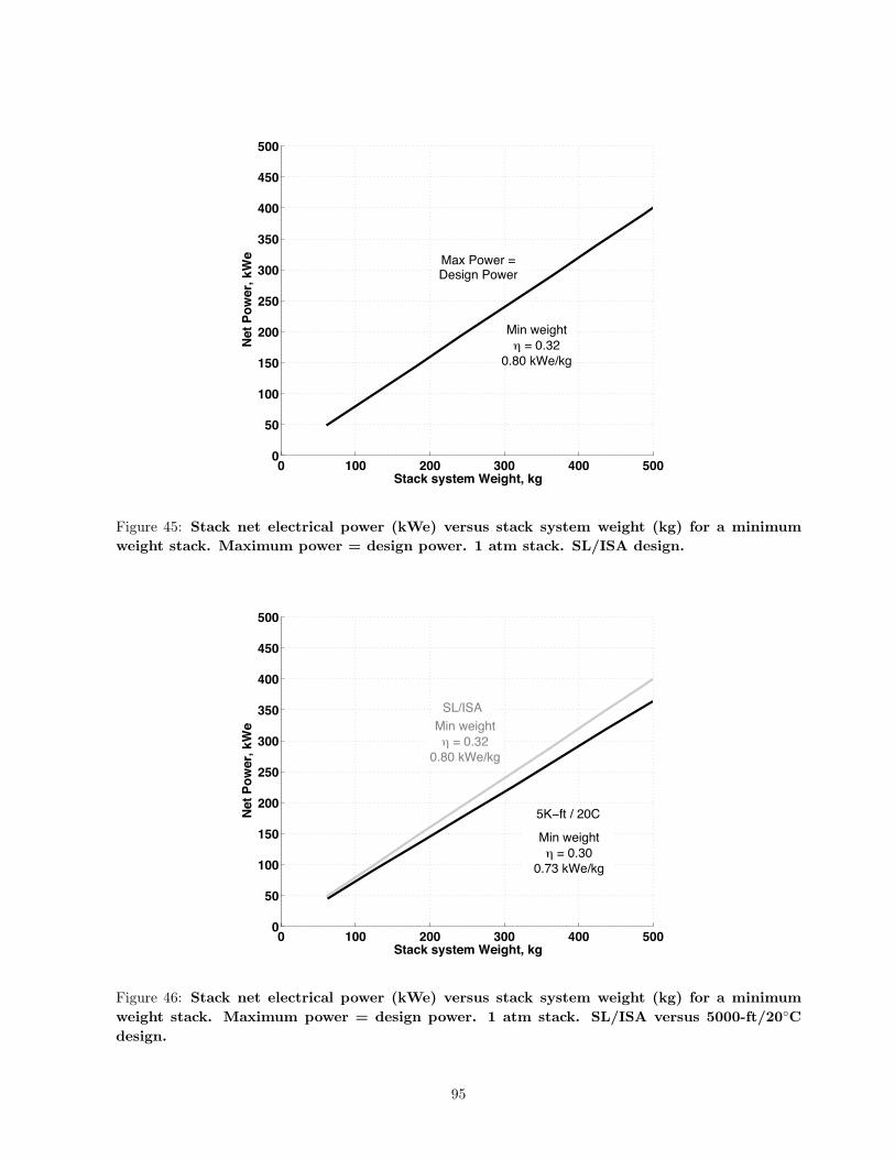
0 100 200 300 400 5000
50
100
150
200
250
300
350
400
450
500
Stack system Weight, kg
Net
Pow
er, k
We
Max Power =Design Power
Min weightη = 0.32
0.80 kWe/kg
Figure 45: Stack net electrical power (kWe) versus stack system weight (kg) for a minimumweight stack. Maximum power = design power. 1 atm stack. SL/ISA design.
0 100 200 300 400 5000
50
100
150
200
250
300
350
400
450
500
Stack system Weight, kg
Net
Pow
er, k
We
5K−ft / 20C
Min weightη = 0.30
0.73 kWe/kg
SL/ISAMin weightη = 0.32
0.80 kWe/kg
Figure 46: Stack net electrical power (kWe) versus stack system weight (kg) for a minimumweight stack. Maximum power = design power. 1 atm stack. SL/ISA versus 5000-ft/20Cdesign.
95

0 100 200 300 400 5000
50
100
150
200
250
300
350
400
450
500
Stack system Weight, kg
Net
Pow
er, k
We
WH
Lower power
Design Power
Max Powerη = 0.29
1.22 kWe/kg
Max efficiencyη = 0.37
0.76 kWe/kg
WL
Higher power
Figure 47: Stack net electrical power (kWe) versus stack system weight (kg) for a maximumefficiency stack. Maximum power > design power. 1 atm stack. SL/ISA design.
0 100 200 300 400 5000
50
100
150
200
250
300
350
400
450
500
Stack system Weight, kg
Net
Pow
er, k
We
SL/ISA
5K−ft / 20Cη = 0.28
1.09 kWe/kgDesignpower
Maxpower
η = 0.350.69 kWe/kg
5K−ft / 20 C
Figure 48: Stack net electrical power (kWe) versus stack system weight (kg) for a maximumefficiency stack. Maximum power > design power. 1 atm stack. SL/ISA vs 5000-ft/20Cdesign.
96

14 Rotorcraft Sizing
A simple sizing method is presented. The objective is to illustrate how the fuel cell models enter and affectsizing, and how it compares with other powerplants, namely, batteries and piston-engines. The model iskept deliberately simple, with a minimal set of parameters, so it can be reproduced easily and might serveas a common-basis for assessment by fuel cell, hydrogen, and rotorcraft specialists.
The sizing problem is defined as the following.Given — Mission and payload WPAY .Find — Design gross weight W and engine power P .The mission is generally described in segments, with environment, reserves, power factors and flight tasks
defined for each segment. For simplicity, only two segments are considered, a hover and a cruise segment.The principal design variable is the disk loading DL. DL = W/A (lb/ft2 or N/m2) where W is the
rotorcraft gross take-off weight (lb or N) and A (ft2 or m2) is the projected disk area of all lifting rotorsthat balance the weight. If there are NR identical rotors of radius R (ft or m), the projected disk area isA = NR πR2. Disk loadings of 8 and 14 lb/ft2 are typical of large helicopters and tiltrotors respectively,whereas 2 − 4 lb/ft2 are typical of small light-utility helicopters.
The sizing method finds the gross weight and engine power for a specified disk loading. The disk loadingis then varied to span the design space.
The sizing method begins with an initial estimate of W , calculates aircraft power, calculates the weightsof all subsystems based on this power, adds them to obtain a new aircraft weight, and iterates the newweight until convergence. The subsystem models keep account of the running weight of the aircraft due tofuel burn or payload change. Here, weight changes during the mission are ignored.
The hover Figure of Merit FM and cruise lift to drag ratios L/D are required. These are the efficiencymetrics in hover and cruise.
FM = 0.7 − 0.8 for all rotorcraft. FM < 1.0.L/D = 4 − 6 for helicopters and compounds and 7 − 9 for tiltrotors.If the configuration is known, FM and L/D can be calculated and updated within the weight iteration.
14.1 Basic Sizing
Specify a disk loading DL, hover power factor PF , air density ρ, and cruise speed V .Assume FM in hover out of ground effect (OGE) and L/D in cruise.Starting from an initial gross take-off weight W , iterate the following steps to converge.
1. Calculate hover power out of ground effect (OGE) PH and engine power P
PH =1
FMW
√
DL
2 ρ
P = PH × PF
(127)
The power factor PF ≥ 1 is a specified margin.
The unit of ρ is kg/m3 if W is in N, or slug/ft3 if W is in lb.
2. From DL and number of rotors, find rotor radius R.
97

3. Calculate cruise power PC at the specified cruise speed V
PC =W V
L/D(128)
4. Calculate structural weight WS
WS = fS W (129)
The factor fS is very difficult to determine yet it can make or break a design. This is where full-scale prototype testing becomes essential for a new kind of aircraft. Historical trends of conventionalhelicopters indicate fS = 0.25 is a good target to aspire (Harris 2012).
5. Calculate power plant weight WP and fuel weight WFuel.
The engine models are from Harris 2012 and the motor model from Ng and Datta 2019.
Turboshaft: WP in lb = 1.8 (P in hp)0.9
Piston: WP in lb = 6.5 (P in hp)0.9
Electric motor: WP in kg = 0.4 (Q in Nm/η)0.71
(130)
where Q is the motor torque and η is motor efficiency.
The fuel weight models are
Turboshaft: WFuel in lb = SFC in lb/hp-hr × E in hp-hr
Piston: WFuel in lb = SFC in lb/hp-hr × E in hp-hr
Battery: WBatt in kg =EB in Wh
Specific Energy SE in Wh/kg
(131)
The specific fuel consumption (SFC) varies from turboshaft to piston. E is the mission energy. If SFCvaries from hover to cruise then the calculations are performed accordingly using energy in hover andcruise (EH and EC). In general, engine charts provide SFC as a function of power.
The battery energy EB requires calculation of C-rates ζ (1/hr). If hH and hC are the hover and cruisetimes in hours, including reserves, then the energy and required C-rates are
EH = hH PH
EC = hC PC
E = EH + EC
ζH =PH
E=
1
hH + (PC/PH)hCor 0 if hH = 0
ζC =PC
E=
1
(PH/PC)hH + hCor 0 if hC = 0
(132)
If the required C-rates are within the maximum available C-rate ζmax then EB = E. Otherwise EB =P/ζmax where P is the higher power. In this case, more energy is carried than needed. For example,if only 5 min of hover is needed, i.e. 1/12 hr, then the required C-rate in hover is ζH = PH/EH = 12.If the available C-rate is only 6, then ζH = PH/EH = 6, or EH =(1/6) PH , which means the batterymust be sized for 1/6 hr of hover, i.e. 10 min, even when only 5 min were needed.
The specific energy SE (Wh/kg) of current Li-ion batteries is approximated by Ng and Datta 2019
SE =vc Cc
(0.0075 + 0.024 Cc) fT≈
vc
0.024 fT(133)
98
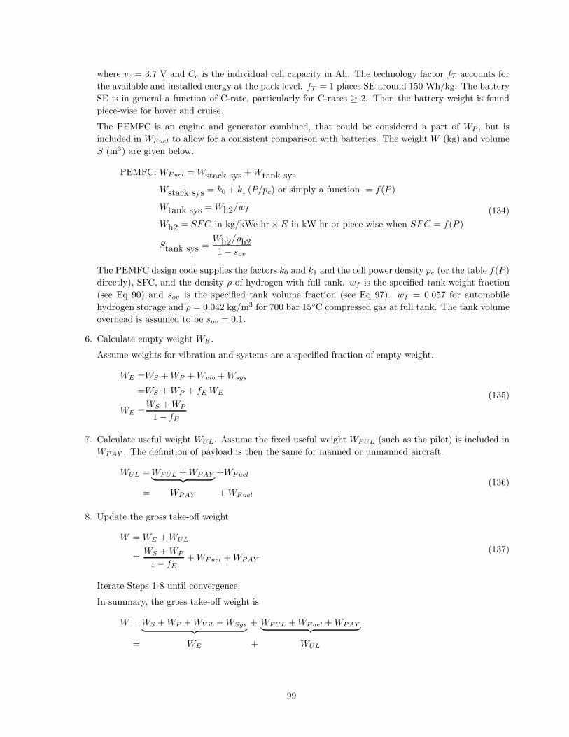
where vc = 3.7 V and Cc is the individual cell capacity in Ah. The technology factor fT accounts forthe available and installed energy at the pack level. fT = 1 places SE around 150 Wh/kg. The batterySE is in general a function of C-rate, particularly for C-rates ≥ 2. Then the battery weight is foundpiece-wise for hover and cruise.
The PEMFC is an engine and generator combined, that could be considered a part of WP , but isincluded in WFuel to allow for a consistent comparison with batteries. The weight W (kg) and volumeS (m3) are given below.
PEMFC: WFuel = Wstack sys + Wtank sys
Wstack sys = k0 + k1 (P/pc) or simply a function = f(P )
Wtank sys = Wh2/wf
Wh2 = SFC in kg/kWe-hr× E in kW-hr or piece-wise when SFC = f(P )
Stank sys =Wh2/ρh21 − sov
(134)
The PEMFC design code supplies the factors k0 and k1 and the cell power density pc (or the table f(P )directly), SFC, and the density ρ of hydrogen with full tank. wf is the specified tank weight fraction(see Eq 90) and sov is the specified tank volume fraction (see Eq 97). wf = 0.057 for automobilehydrogen storage and ρ = 0.042 kg/m3 for 700 bar 15C compressed gas at full tank. The tank volumeoverhead is assumed to be sov = 0.1.
6. Calculate empty weight WE .
Assume weights for vibration and systems are a specified fraction of empty weight.
WE =WS + WP + Wvib + Wsys
=WS + WP + fE WE
WE =WS + WP
1 − fE
(135)
7. Calculate useful weight WUL. Assume the fixed useful weight WFUL (such as the pilot) is included inWPAY . The definition of payload is then the same for manned or unmanned aircraft.
WUL =WFUL + WPAY︸ ︷︷ ︸
+WFuel
= WPAY + WFuel
(136)
8. Update the gross take-off weight
W = WE + WUL
=WS + WP
1 − fE+ WFuel + WPAY
(137)
Iterate Steps 1-8 until convergence.
In summary, the gross take-off weight is
W = WS + WP + WV ib + WSys︸ ︷︷ ︸
+ WFUL + WFuel + WPAY︸ ︷︷ ︸
= WE + WUL
99

Also
W = WS + WP + WV ib + WSys + WFUL + WFuel︸ ︷︷ ︸
+ WPAY
= WO + WPAY
where WO is the operating weight.
The gross take-off weight W is also denoted by WGTO. WGTO for the primary mission is the designgross weight denoted by WD.
14.2 Essential Refinements
While the basic sizing gives a crude assessment of whether the aircraft can lift off the ground, for realisticassessment, the following refinements are essential.
1) FM in Step 1 should be calculated and updated every iteration,2) L/D in Step 3 should be calculated and updated every iteration,3) Step 4 should include rotor weight with dependence on flapping frequency, and4) Step 5 should be combined with a gear-box.
Refinement 1: Hover Figure of Merit (FM)
The calculation of FM requires the additional inputs: tip Mach number MT , solidity σ, an induced powerfactor κ, an average airfoil lift curve slope clα and a mean airfoil drag coefficient cd0.
As W is updated (thrust T = W ), the ideal and actual powers Ph and PH can be calculated. Their ratiois the FM. The ideal power is the ideal induced power
Ph = W
√
DL
2 ρ=
W 1.5
√2 ρ A
The actual power is the true induced power κh Ph where κh is the induced power factor (≈ 1.05− 1.15) andthe profile power from drag of the blades.
PH = κhW 1.5
√2 ρ A
+1
8σ cd0 ρ A (ΩR)3
Thus
FM =Ph
PH=
W 1.5√
2 ρ A
κhW 1.5√
2 ρ A+ 1
8 σ cd0 ρ A (ΩR)3(138)
The tip speed ΩR = MT as were as is the speed of sound. The solidity is the ratio of blade area to diskarea σ = Ab/A. The blade area is written as Ab = Nb c R where Nb is the number of blades and c is a meanchord, so σ = Nb c/πR.
The power loading PL = W/PH (lb/hp) is then
PL =FM
PF
√
2 ρ
DL(139)
Figure 49 shows measured PL versus DL of current rotorcraft. The maximum engine installed power P isused in the plot, so the constant FM curves are really constant FM/PF curves.
100

Also needed is the thrust coefficient
CT =T
ρ A (ΩR)2
and the blade loading CT /σ. The mean airfoil lift coefficient cl is related to this parameter
cl = 6CT
σ
The mean airfoil angle of attack is then cl/clα. The mean angle of attack must remain below stall forsensible results. Therefore, a maximum CT /σ is specified (normally ≈ 0.12), and if the updated W exceedsthis limit, the solidity σ is increased, by increasing the mean chord of the blade. The wider chord enters therotor weight model.
Free-wake analysis and measured or 2D-CFD calculated airfoil decks are needed for proper estimates ofκ and cd0 which are then input into the analysis. Or, Mach-scaled model rotors (same tip Mach number asfull-scale) are hover tested to identify these constants.
0 5 10 15 20 250
2
4
6
8
10
12
14
16
Disk loading, lb/ft2
Pow
er lo
adin
g, lb
/hp
HelicopterTandemCoaxialTiltrotor
0.6
0.40.5
Figure of Merit
Figure 49: Power loading versus disk loading of rotorcraft. Engine installed power and take-offweight are used.
Refinement 2: Cruise Lift-to-Drag (L/D)
The calculation of L/D requires the additional input: the drag of the fuselage without the rotor blades(but including the hub). The fuselage drag DF is expressed as
DF = 1/2 ρ V 2 F
101

where F is a drag area. The drag area in ft2 can be approximated for existing rotorcraft by the Harris curve
F = f
(W in lb
1000
)2/3
where the factor f ≈ 4.2 on average for all helicopters from 2, 000− 40, 000 lb, but ≈ 2.6 for a modern civilhelicopter with retractable landing gear, and even lower ≈ 1.5 for a tiltrotor.
The power required by a rotorcraft in level equilibrium flight is composed of rotor induced power (togenerate lift, subscript i), rotor profile power (to overcome drag of the rotating blades, subscript o) and thepropulsive power required to overcome drag (subscript p), DF V .
P = Pi + Po + DF V
The lift-to-drag ratio is
L/D =W
P/V(140)
The coefficient of power is
CP =P
ρ A (ΩR)3
Helicopter:For a helicopter, the coefficients of power are the following.
CPi = κf λi CT
where
λi =CT
2√
µ2 + λ2is the induced inflow
µ = V cosαS/ΩR is the advance ratio
αS ≈ tan−1 DF /W is the rotor shaft tilt forward
λ = V sin αS/ΩR + λi = µ tan αS + λi is the total inflow
CT =T
ρ A (ΩR)2where rotor thrust T ≈
(
D2F + W 2
)1/2
CPo = 1/8 σ cd0 (1 + 4.65 µ2)
CPp =DF V
ρ A (ΩR)3= 1/2
µ3
cos3 αS
F
A≈ 1/2 µ3 F
Afor αS < 10
(141)
All together
CP = κfC2
T
2√
µ2 + λ2+ 1/8 σ cd0 (1 + 4.65 µ2) + 1/2 µ3 F
A
Given aircraft weight W , fuselage drag area F , rotor tip speed, solidity, disk area, and airfoil drag, thepower can be calculated at any speed. κf is the induced power factor in cruise and can be used to accountfor non-uniform inflow, wake distortion and interference losses. The classical approximation to accountfor non-uniform inflow is κf ≈ 1.15. The effective drag coefficient cd0 can be calibrated to higher-fidelitypredictions.
102

The inflow
λ = µ tan αS + λi where λi =CT
2√
µ2 + λ2is itself a function of λ
requires Newton-Raphson iterations to solve, but a simpler approximation λi ≈ CT/2µ can be used for speedsµ > 0.1 or so. This gives
CP ≈ κfC2
T
2 µ+ 1/8 σ cd0 (1 + 4.65 µ2) + 1/2 µ3 F
A
Compound Helicopter:The same Eq 141 apply with the following changes.For wing/s, the wing drag is added to the fuselage drag and the rotor thrust reduced by a specified wing
lift share.
DF =1/2 ρ V 2
[
F + AW
(
cd0W +c2lW
π AR e
)]
clW =LW
1/2 ρ V 2 AW
T ≈(
D2F + (W − LW )2
)1/2
αS ≈ tan−1 DF /(W − LW )
(142)
AW is the total surface area of the wing, cd0W is its zero-lift drag coefficient and the c2lW term is its lift-
induced drag coefficient. AR is the aspect ratio and e is the Oswald efficiency factor. e < 1 and typically≈ 0.8.
For propeller/s, the propeller profile drag is added and the rotor thrust reduced by a specified propellerthrust share. The propeller profile power Po = propeller CPo × ρ AP (ΩR)3P , where AP and (ΩR)P arethe disk area and tip speed of the propeller. The profile power coefficient of Eq 141 can be used or refinedto Eq 143 given later for tiltrotor. The rotor thrust is reduced by a specified propeller thrust TP , so
T =(
(DF − TP )2 + (W − LW )2)1/2 and αS ≈ tan−1(DF − TP )/(W − LW ).
Given the wing properties — area, aspect ratio, drag coefficient, e, and propeller properties — cd0, tipspeed, and disk area, and specified lift and thrust shares, DF and T can be calculated and inserted in Eq 141to find power.
Tiltrotor:The tiltrotor is a winged compound with the special capability of airplane mode when the rotors are fully
tilted forward.In hover, DF = 0 and T = W . Wing download might increase required thrust by 10− 30% W.In airplane mode cruise, LW = W and T = DF . The wing loading WL = W/AW (lb/ft2) is similar
to disk loading and a typical value is 70 lb/ft2. Specifying a design wing-loading determines the wingarea. Specifying a design wing-loading along with a corresponding design speed, determines the design winglift coefficient clW . Alternatively, specifying a design wing-loading along with a corresponding design liftcoefficient clW , sets the design speed.
103

0 50 100 150 200 2500
1
2
3
4
5
6
7
8
9
Airspeed, kt
Airc
raft
L / D
( =
W V
/ P
)
HelicopterTandemCompoundTiltrotor
LockheedAH−56A
attack prototype
Sik S−67Attack prototype
Bell 209attack prototype
YR−4B
BellXV−15tiltrotor
Sik UH−60AUtility
TransportCoax
XH−59A
Figure 50: Measured L/D of various rotorcraft.
In airplane mode, the coefficients of power are the following.
CPi = κf λi CT
where
λi = −λC
2+
√(
λC
2
)2
+CT
2≈
CT
2 λCand λC =
V
ΩRis the cruise inflow
CT =T
ρ A (ΩR)2where rotor thrust T = DF
CPo = 1/8 σ cd0 FP
where
FP =√
1 + λ2C
(
1 + 5/2 λ2C
)
+ 3/2 λ4C ln
1 +√
1 + λ2C
λC
CPp =DF V
ρ A (ΩR)3= 1/2 λ3
C
[F
A+
AW
A
(
cd0W +c2lW
π AR e
)]
where
clW =LW
1/2 ρ V 2 AW=
WL1/2 ρ V 2
(143)
104

0 50 100 150 200 2500
1
2
3
4
5
6
7
8
9
Airspeed, kt
Airc
raft
L/D
Helicopter
Tiltrotor
Figure 51: Calculated L/D of a helicopter and tiltrotor.
All together
CP = κfC2
DF
2 λC+ 1/8 σ cd0 FP + 1/2 λ3
C
(F
A+
AW
Acd0W
)
+ 1/2 λ3C
AW
A
c2lW
π AR e
In dimensional form
P =
(
κfC2
DF
2 λC+ 1/8 σ cd0 FP
)
ρ A (ΩR)3 +1
2ρ V 3 (F + AW cd0W ) +
W
V
2 WL
ρ
1
π AR e
The rotor induced power is negligible in airplane mode as C2DF /2λC ≈ 0.
At speeds slower than the design speed, the lift coefficient of the wing must increase for wing lift to stillsupport the weight, so the aircraft must pitch up. The pitch angle θ also tilts the rotor thrust up so it mustnow equal T = DF / cos θ. The lifting component of this thrust, LR = T sin θ, reduces the lift required fromthe wing, so really LW = W − LR. The lift coefficient can be iterated to find the right pitch angle at whichthe wing and the rotor lifts balance the weight. Normally for pitch angles θ < 10 this iteration can beignored as LR << W . Regardless, the results is that a slight pitch up of the aircraft usually produces atbetter L/D. The tiltrotor data in Fig 50 (from XV-15) shows this peak around 150 kt.
Example calculations are shown in Fig 51. The examples consist of two aircraft of same gross weightW = 5000 lb, flying at SL/ISA with air density ρ = 0.00237 slug/ft3, and speed of sound aS = 1100 ft/s. Therotor properties are the same: tip Mach number MT = 0.5 (lower than the typical ≈ 0.65 to reduce noise),solidity σ = 0.06, induced power factor κf = 1.15, and airfoil mean profile drag coefficient cd0 = 0.008.For the helicopter, the Harris drag factor f = 4.2 and disk loading DL = 2.5 lb/ft2. For the tiltrotor, the
105

Harris drag factor f = 1.5 and disk loading DL = 13 lb/ft2. Additional inputs for the tiltrotor are the wingproperties: design wing loading WL = 70 lb/ft2, design speed V = 250 kt, wing mean profile drag coefficientcd0W = 0.01, aspect ratio AR = 8, Oswald efficiency e = 0.8, and airfoil mean lift curve slope clα = 5.73.The pylon is always down. Below 100 kt the wing stalls due to the high pitch of the aircraft; in practice,flaps are deployed to increase lift coefficient, which typically brings down the L/D below a helicopter. Thespeed of peak L/D is a function of the tip speed (i.e. tip Mach number) either through the advance ratio µ(helicopter) or the inflow ratio λC (tiltrotor).
The simple expressions are based on energy balance in equilibrium flight without regard to how theequilibrium is achieved (trim solution) or whether it can in fact be achieved (stall limit). The many underlyingassumptions used to arrive at these closed form expressions are too simplistic. Some of them, such as uniforminflow, uniform chord, linear lift, and constant drag can be accounted for by calibrating the coefficientsκ, cd, cl, e to flight test data. Some, such as, compressibility, stall, 3D effects and interference require higher-fidelity lifting-line analysis. The simple analysis also assumes all NR rotors operate at the same state.
The measured L/D = WV/P of current rotorcraft is compiled in Fig 50. Compounds buy higher speedswithout significant low speed penalty. Tiltrotors buy very high speed with significant low speed penalty.The penalty leads to higher structural weight fraction fS .
In a tiltrotor, reducing tip speed ΩR in cruise to 50% of hover, reduces power and improves L/Dsignificantly. An electric motor is capable of this reduction with less than 15% loss in efficiency. The turbo-shaft limit is around 15− 20% reduction in ΩR (the V-22). Ng and Datta 2019 predicts L/D ≈ 10− 11 with50% reduction in tip speed, with a refined trim analysis and airfoil decks, see Fig 52. The 50% reduction wasthe limit beyond which the rotor stalled and there was no gain. This is an exclusive advantage of electricpower and a tiltrotor with high cruise speed can take advantage of it.
Figure 52: Predicted L/D of an electric tiltrotor with 50% rotor tip speed reduction in cruise.
106

Refinement 3: Rotor Weight
The structural weight calculation in Step 4 should be refined to calculate rotor weights. Even thoughthere are no production eVTOL, there is a rich variety of production rotors, and the historical weights fromthese rotors are a reliable basis on which to predict rotor weights. Rotor weights vary with rotor radius,chord, and flapping frequency and these variations must be accounted for in the weight iteration.
The weight of each rotor is calculated using the U.S. Army AFDD82 model which calculates the weightof all blades (7.7% average error based on 37 aircraft) and the hub (10.2% average error based on 35 aircraft)in lb.
Wb = χb 0.02606 N0.6592b R1.3371 c0.9959 (ΩR)0.6682 ν2.5279
β
Wh = χh 0.003722 N0.2807b R1.3371 (ΩR)0.4290 ν2.1414
h W 0.5505b
WR = Wb + Wh
(144)
whereνβ in /rev is the blade flapping frequency (rad/s) divided by rotational speed Ω (rad/s),νh in /rev is the hub frequency (= νβ , or collective frequency for teetering rotors),Nb is the number of blades,c and R are the mean chord and radius respectively in ft,and ΩR is the tip speed in ft/s.The χ are calibration or technology factors (< 1 for future advanced rotor assumption).The structural weight WS in step 4 is now changed to
WS = NR WR + fS W
where fs is now the weight fraction of the rest of the aircraft without the rotors.
Refinement 4: Gear-box
Inclusion of a gear-box in Step 5 changes the electric motor equation in Eq 130 and adds a gear-boxweight. Gear-boxes are far more torque dense than electric motors. They also absorb the intense rotorvibratory loads that might otherwise break the motors.
The weight of the gear box and rotor shaft is calculated using the U.S. Army AFDD83 model (7.7%average error based on 30 aircraft).
WP in kg = 0.4
(Q in Nm
GR ηg η
)0.71
WG in lb = 57.72 (P in hp)0.8195 f0Q.068 n0.0663
g
(Motor RPM
1000
)0.037 1
Rotor RPM0.638
(145)
where ηg is the gear box efficiency, GR is the gear ratio (Motor RPM/Rotor RPM), fQ is a constant, and ng
is the number of gear boxes (= 1 for eVTOL for each motor/rotor). The total weight is found by multiplyingwith the number of rotors NR. fQ represents the second rotor torque limit in %. fQ = 60 for twin rotorsand 3 for single main-rotor and tail-rotor.
A conservative model for efficiency is used, valid for GR < 100.
ηg = 1 −GR
100
These are crude trends and should be used with caution. The gear-ratio can be increased to very highnumbers, since there is no mechanical limit on the gear-speed or heat limit on the motor. The motorequation is derived from permanent magnet motors whereas the gear box equation is from conventionalturbo-shaft helicopters.
107

14.3 Example: NASA Electric Quad-rotor
The NASA electric quad-rotor is a battery-powered single-occupant conceptual design by Johnson, Silva andSolis 2018 and Johnson and Silva 2018.
The original work used NASA Design and Analysis of Rotorcraft software with detailed modeling of manysubsystems. Here, the method described earlier in the section on Rotorcraft Sizing / Essential Requirementsis used. The Figure of Merit is calculated using Eq 138. The helicopter power and L/D are calculated usingEq 140 and 141 respectively. The basic trends can be reproduced with a small number of inputs listed below.
The conditions are 5000-ft ISA + 20C which give the following.Air density ρ = 0.0019438 slug/ft3 (1.0018 kg/m3)Speed of sound as = 1132 ft/s (345 m/s)
The sizing mission is given by the following.Payload = 250 lb (including pilot)Hover OGE = 4 minCruise speed for best range = Vbr ≈ 70 knot (36 m/s), so this speed is specified for all designsCruise reserve = 20 min
The aircraft inputs are the following.Disk loading = 2.5 lb/ft2
Fraction structural weight fS = 0.20Fraction vibration and systems weight fE = 0.15Harris drag factor f = 2.95Number of rotors = 4
The rotor inputs are the following.Number of blades per rotor = 3Tip Mach number MT = 0.4 (tip speed = 138 m/s)Solidity = 0.0646Airfoil mean drag coefficient cd0 = 0.009Airfoil mean lift curve slope clα = 5.73 per radianκh = 1.15κf = 1.15Flapping frequency νβ = 1.125 / revHub frequency νh = νβ
Blade tech factor = 0.5Hub tech factor = 0.5
The power system inputs are the following.Power factor PF = 1.5RPM motor = 1000η Motor = 0.80Fraction controller and power conditioner weight = 0.5Fraction cooling system weight = 0.5fQ = 60ng = 1Battery Wh/kg available and installed = 150, 200, 300, 400Battery Max C-rate = unlimited
108

Figures 53 and 54 show the gross weight and hover power respectively varying with range for a batterypowered aircraft. There is a mis-match in predictions at higher battery specific energies, but they match atthe lower levels. The lower levels are closer to the state-of-the-art. Note that the specific energy are at thepack level, installed and available (80% discharge, end-of-life) values.
The batteries are now replaced with PEMFC. A 2.5 atm modern stack sized for maximum efficiencyis used. The power versus weight was shown in Fig 40 and specifications for a 500 kWe design given inTable 29 column 5. The tank specifications were 5.7% weight fraction filled to 700 bar 15C with 10%overhead for structural volume. Figure 55 shows the design gross weight varying with range. If the stack issized to deliver the maximum aircraft power (1.5× hover power OGE) as design power (cooling system sizedto design power) the higher solid line is obtained. If the stack is sized to deliver the maximum aircraft poweras maximum power (cooling system sized to design power) then the lower dashed line is obtained. This isthe more appropriate design as the power factor of 1.5 places the hover power near and slightly below thedesign power ensuring continuous hover. This is still an over design as only 4 min of hover is required. ThePEMFC solution surpasses the 200 Wh/kg battery solution above a range of 60 nm (produces a lighter andsmaller aircraft). The barrier is the 400 L tank volume seen in Fig 56. These solutions are representative ofmodern automobile fuel cell technology.
In eVTOL, short-term hydrogen storage is envisioned to allow greater hydrogen weight fractions. Thedramatic impact of increasing hydrogen weight fractions from 5.7 to 7.5 to 15% is evident in both the figures.At 15% weight fraction, a range of 125 nm is possible with an aircraft of 2750 lb. About 35 lb of hydrogenwould be needed to fly this range, so the tank volume remains very high at 450 L. If a 1 atm stack is usedinstead of a 2.5 atm stack, the predictions change significantly. The power versus weight of a 1 atm stackwas shown in Fig 48 and specifications for a 500 kWe design given in Table 29 column 7. Figure 57 and 58show the gross weight and tank volumes with 1 atm stacks. The PEMFC solution now overtakes the 200Wh/kg battery solution above a range of 25 nm and the 300 Wh/kg battery solution above 85 nm. Thecorresponding tank volumes are shown in Fig 58. At 15% weight fraction, a range of 125 nm is now possiblewith an aircraft of only 2000 lb. About 20 lb of hydrogen would be needed to fly this range, so the tankvolume is reduced to only 260 L.
Quantitative conclusions are premature without calibrations from an actual flight test aircraft (or aflight-worthy test bed), but the trends are clear, and they reveal the key technology drivers. These are:1) high weight fraction hydrogen storage up to at least 15%, and 2) power-to-weight ratios greater than1.0 kWe/kg for the stack system (stack plus ancillary subsystems). The unique attributes of an eVTOL— short hover, short hydrogen storage (2-3 hrs), and low altitude near 1-atm flight should be leveraged toopen opportunities for achieving these targets. The downwash from the rotors should be leveraged to pursueavenues for lighter stack cooling.
109

0 25 50 75 100 125 150 175 2000
1000
2000
3000
4000
5000
6000
Range, n−miles
Wei
ght,
lb
NASA
150 Wh/kg
200 Wh/kg
300 Wh/kg
400 Wh/kg
UMD
Figure 53: Gross weight versus range with batteries. Electric quad-rotor. 250 lb payload.Battery specific energy are pack-level available and installed values.
0 25 50 75 100 125 150 175 2000
50
100
150
200
250
300
350
400
450
Range, n−miles
Hov
er p
ower
, hp
150 Wh/kg
400 Wh/kg
200 Wh/kg 300
Wh/kg
NASA
UMD
Figure 54: Hover power versus range with batteries. Electric quad-rotor. 250 lb payload.Battery specific energy are pack-level available and installed values.
110

0 25 50 75 100 125 150 175 2000
1000
2000
3000
4000
5000
6000
Range, n−miles
Wei
ght,
lb
150 300 400 Wh/kg
200
PEM FC
BATTERIES
H2 7.5%
H2 15%
Hover P x PF = Max FC P0.83 kWe/kg H2 5.7%
Hover P x PF = Dsg FC P0.56 kWe/kg H2 5.7%
Figure 55: Gross weight versus range with 2.5 atm PEMFC sized to deliver 1.5× hover poweras design power (solid line) and maximum power (dashed line). Hydrogen wt% 5.7, 7.5 and15. Electric quad-rotor. 250 lb payload.
0 25 50 75 100 125 150 175 2000
100
200
300
400
500
600
Range, n−miles
H2
tank
vol
ume,
L
700 bar 15 C@ 0.0362 kg/L
Hover P x PF = Max FC P0.83 kWe/kg H2 5.7%
48 lbH2
28 lbH2
Hover P x PF = Dsg FC P0.56 kWe/kg H2 5.7%
H2 7.5%
H2 15%
Figure 56: Tank volume versus range with 2.5 atm PEMFC sized to deliver 1.5× hover poweras design power (solid line) and maximum power (dashed line). 2.5 atm stacks. 700 bar 15
C tank. Hydrogen wt% 5.7, 7.5 and 15. Electric quad-rotor. 250 lb payload.
111

0 25 50 75 100 125 150 175 2000
1000
2000
3000
4000
5000
6000
Range, n−miles
Wei
ght,
lb
150 200 400 Wh/kg
Hover P x PF = Dsg FC P0.69 kWe/kg H2 5.7%
Hover P x PF = Max FC P1.09 kWe/kg H2 5.7%
H2 15%
H2 7.5%
PEM FC
BATTERIES
300
Figure 57: Tank volume versus range with 1 atm PEMFC sized to deliver 1.5× hover power asdesign power (solid line) and maximum power (dashed line). 700 bar 15 C tank. Hydrogenwt% 5.7, 7.5 and 15. Electric quad-rotor. 250 lb payload.
0 25 50 75 100 125 150 175 2000
100
200
300
400
500
600
Range, n−miles
H2
tank
vol
ume,
L
700 bar 15 C@ 0.0362 kg/L
48 lbH2
Hover P x PF = Dsg FC P0.69 kWe/kg H2 5.7%
Hover P x PF = Max FC P1.09 kWe/kg H2 5.7%
H2 7.5%
H2 15%
35 lbH2
Figure 58: Tank volume versus range with 1 atm PEMFC sized to deliver 1.5× hover poweras design power (solid line) and maximum power (dashed line). 700 bar 15 C at full tank.Hydrogen wt% 5.7, 7.5 and 15. Electric quad-rotor. 250 lb payload.
112
14.4 Example: Maryland Electric Quad-rotor
The Maryland electric quad-rotor is a battery-powered two-occupant conceptual design by Fisler and Datta2020. It follows the NASA quad-rotor, only carries a higher payload of 400 lb, equal to the payload of theR22 Beta II helicopter.
The method described earlier in the section on Rotorcraft Sizing / Essential Requirements is used. TheFigure of Merit is calculated using Eq 138. The helicopter power and L/D are calculated using Eq 140 and141 respectively. The changes in inputs from the NASA quad-rotor are the payload (400 lb instead of 250lb), the Harris drag factor f (3.95 instead of 2.95), and a stall limit on the blade loading (CT /σ ≤ 0.12).
The conditions are 5000-ft ISA + 20C which give the following.Air density ρ = 0.0019438 slug/ft3 (1.0018 kg/m3)Speed of sound as = 1132 ft/s (345 m/s)
The sizing mission is given by the following.Payload = 400 lb (increased)Hover OGE = 4 minsCruise speed = Vbr ≈ 70 knot (118 ft/s) so this speed is specified for all designsCruise reserve = 20 min
The aircraft inputs are the following.Disk loading = 2.5 lb/ft2
Fraction structural weight fS = 0.20Fraction vibration and systems weight fE = 0.15Harris drag factor f = 3.95 (increased)Number of rotors = 4
The rotor inputs are the following.Number of blades per rotor = 3Tip Mach number MT = 0.4 (tip speed = 138 m/s)Solidity = 0.0646Airfoil mean drag coefficient cd0 = 0.0090Airfoil mean lift curve slope clα = 5.73 per radianκh = 1.15κf = 1.15Flapping frequency νβ = 1.125 / revHub frequency νh = νβ
Blade tech factor = 0.5Hub tech factor = 0.5Maximum CT /σ = 0.12 (stall limit)
The power system inputs are the following.Power factor PF = 1.5RPM motor = 1000η Motor = 0.80Fraction controller and power conditioner weight = 0.5Fraction cooling system weight = 0.5fQ = 60ng = 1
113
Battery Wh/kg available and installed = 150, 200, 300, 400Battery Max C-rate = unlimited, 2
Figure 59 shows the gross weight varying with range for a battery powered aircraft. Figure 60 shows thecorresponding C-rates. The 150 and 200 Wh/kg values are near the state-of-the-art specific energy at packlevel, installed and available (80% discharge, end-of-life). The C-rates required for a range of 25 nm are 2.5Cin hover and 1C in cruise. The required C-rates are set by the hover time and range, hence independentof specific energy of the batteries, a requirement that is typically at odds with electrochemistry where theavailable C-rates typically diminish with specific energy. The plots show, higher energy batteries (200 or300 Wh/kg) enable greater range for the same aircraft weight, or lighter aircraft for the same range. Thelatter appears to be the more effective option. If however, higher energy comes at the cost of lower C-rate,flying a greater range might be the only option. These options impact infrastructure. Thus, aircraft andinfrastructure are tied to the trajectory of battery technology.
The batteries are now replaced with PEMFC. Figure 61 shows the gross weight versus range with threetypes of designs — two with 2.5 atm stacks and one with a 1 atm stack. All are sized for maximumefficiency. The tank specifications for all are 5.7% weight fraction filled to 700 bar 15C with 10% overheadfor structural volume. First consider the 2.5 atm stack. If it is sized to deliver the maximum aircraft power(1.5× hover power OGE) as the design power the higher solid line in the farthest corner is obtained. If thestack is sized to deliver the maximum aircraft power as maximum power (cooling system sized to designpower) then the lower solid line is obtained. This is the more appropriate design as the power factor of1.5 places the hover power near or slightly below the design power ensuring continuous hover. If the 1 atmstack is used, the weights are lowered significantly, showing the potential benefits of low altitude flight. Thecorresponding tank volumes are shown in Fig 62. These solutions are representative of modern automobilefuel cell technology.
For comparison, the piston engine R22 Beta II gross weight (1371 lb), range (180 nm), and fuel tankvolumes (100 L), are plotted. As expected, these are located far below the electric power plants.
In eVTOL, short-term hydrogen storage is envisioned to allow greater hydrogen weight fractions. Theeffect of weight fraction is shown in Fig 63. Increasing weight fraction flattens the curve up to 15%, beyondwhich there is a diminishing return. Figure 64 shows the effect of stack system power-to-weight. Increasingpower-to-weight lowers the curve up to 1.5 kWe/kg beyond which there is a diminishing return. Thus, fora 400 lb payload, 15% weight fraction and 1.5 kWe/kg power-to-weight appear to be effective targets. Theremaining difference from the R22 is largely due to the quad-rotor configuration, not the power plant.
The effect of hydrogen weight fraction on tank volume is shown in Fig 65. Increasing weight fractionreduces the gross weight and the amount of hydrogen needed and therefore the volume. At 15%, 44 lb ofhydrogen is needed to fly the R22 range, which implies a 550 L tank. Figure 66 shows that storage pressurehas a limited impact on tank volume beyond 700 bar. From 700 bar to 800 bar there is a gain of only 50 L.Temperature has a greater impact. From 15C to −150C the volume is halved and equals to that of liquidhydrogen. However, these are not available options with the current infrastructure.
Quantitative conclusions are premature without calibrations from an actual flight aircraft (or a flight-worthy test bed), but the trends are clear, and they reveal the key technology drivers. These are refinedfrom the previous section to include: 1) high weight fraction hydrogen storage of at least 15—30%, 2) power-to-weight ratios of at least 1.0—1.5 kWe/kg for the stack system (stack plus ancillary subsystems), and 3)achieve storage tank temperatures of −50C or lower.
114

0 25 50 75 100 125 150 175 2000
1000
2000
3000
4000
5000
6000
Range, n−miles
Wei
ght,
lb
150 200
BATTERIES
300 Wh/kg(2C)
R22Beta II
Figure 59: Gross weight versus range with batteries. Electric quad-rotor. 400 lb payload.Specific energy are pack-level available and installed values.
0 25 50 75 100 125 150 175 2000
0.5
1
1.5
2
2.5
3
3.5
4
4.5
Range, nm
Bat
tery
C−r
ate
(1/h
r)
150
200
300 Wh/kg(2C)
HOVER
CRUISE
Figure 60: Required C-rate versus range with batteries. Electric quad-rotor. 400 lb payload.Specific energy are pack-level available and installed values. Dotted: hover. Solid: cruise.
115

0 25 50 75 100 125 150 175 2000
1000
2000
3000
4000
5000
6000
Range, n−miles
Wei
ght,
lb
Hover P x PF = Dsg FC P0.56 kWe/kg, 2.5atm
Hover P x PF = Max FC PkWe/kg 0.83, 2.5 atm
Hover P x PF = Max FC PkWe/kg 1.09, 1.0 atm
200 150 300 Wh/kg(2C)
BATTERIES
R22Beta II
Figure 61: Gross weight versus range with 2.5 atm and 1 atm PEMFC sized to deliver 1.5× hoverpower as design power (solid line) or as maximum power (dashed line). Electric quad-rotor.400 lb payload. Hydrogen wt% 5.7.
0 25 50 75 100 125 150 175 2000
100
200
300
400
500
600
Range, nm
H2
tank
vol
ume,
L
Hover P x PF = Max FC P1.09 kWe/kg 1 atm
Hover P x PF = Max FC P0.83 kWe/kg 2.5 atm
700 bar 15 C@ 0.0362 kg/L
Hover P x PF = Dsg FC P0.56 kWe/kg 2.5 atm
R22Beta II
Figure 62: Tank volume versus range with 2.5 atm and 1 atm PEMFC sized to deliver 1.5× hoverpower as design power (solid line) or as maximum power (dashed line). Electric quad-rotor.400 lb payload. Hydrogen wt% 5.7. H2 storage 700 bar 15C.
116

0 25 50 75 100 125 150 175 2000
1000
2000
3000
4000
5000
6000
Range, n−miles
Wei
ght,
lb
BATTERIES
300 Wh/kg(2C)
200 150
Hover P x PF = Max FC PkWe/kg 1.09, 1.0 atm
30%
H2 tank wt7.5%
15%
H2 5.7%
R22Beta II
Figure 63: Gross weight versus range with 1 atm PEMFC sized to deliver 1.5× hover power asmaximum power. Impact of hydrogen wt%. Electric quad-rotor. 400 lb payload. H2 storage700 bar 15C.
0 25 50 75 100 125 150 175 2000
1000
2000
3000
4000
5000
6000
Range, n−miles
Wei
ght,
lb
BATTERIES
300 Wh/kg(2C)
200 150
Hover P x PF = Max FC P1.0 atm, H2 tank wt 15%
kWe/kg1.09
1.50
2.00
R22Beta II
Figure 64: Gross weight versus range with 1 atm PEMFC sized to deliver 1.5× hover power asmaximum power. Impact of stack system specific power. Electric quad-rotor. 400 lb payload.Hydrogen wt% 15. H2 storage 700 bar 15C.
117

0 25 50 75 100 125 150 175 2000
100
200
300
400
500
600
Range, nm
H2
tank
vol
ume,
L
700 bar 15 C@ 0.0362 kg/L
Hover P x PF = Max FC P1.09 kWe/kg, 1.0 atm
15%8%
H2 48 lb
44 lbH2 5.7%
30% 35 lb
R22Beta II
Figure 65: Tank volume versus range with 1 atm PEMFC sized to deliver 1.5× hover power asmaximum power. Impact of hydrogen wt%. Electric quad-rotor. 400 lb payload. H2 storage700 bar 15 C.
0 25 50 75 100 125 150 175 2000
100
200
300
400
500
600
Range, nm
H2
tank
vol
ume,
L
H2 tank wt% 15
Hover P x PF = Max FC P1.09 kWe/kg, 1.0 atm
700b 15 C800b 15 C
800b 0 C800b −50 C800b −150 C
Liq H2
800b −150 C ~= Liq H2
H244 lbfor all
R22Beta II
Figure 66: Tank volume versus range with 1 atm PEMFC sized to deliver 1.5× hover power asmaximum power. Impact of hydrogen storage type. Hydrogen wt% 15. Electric quad-rotor.400 lb payload.
118
14.5 Example: Single Main-Rotor and Tail-rotor
The gap between the R22 and the quad-rotors in the previous sections were due to the configuration. Asingle main-rotor and tail-rotor configuration is sized to bridge this gap.
First, a piston engine helicopter is sized to the R22 Beta II-like specifications: payload 400 lb, range 180nm, and gross weight 1370 lb. Next, the power system is replaced with a PEMFC and an electric motor andgear box. The specific power and hydrogen weight fraction are then varied until the results converge to R22again. The resulting targets are the benchmarks for achieving the objective aircraft.
The 400 lb payload corresponds to a standard tank. The payload and the 20 min cruise reserve (requiredfor VFR) determine the range. It is not clear what this range is; published values vary between 160 nm to208 nm. A range of 180 nm is assumed.
The auxiliary tank flies empty for a 400 lb payload. This is useful in the context of hydrogen storagewhere higher volumes are needed. The standard and the auxiliary tanks have usable volumes of 19.2 and10.5 U.S. gallons respectively. The 19.2 gallon (73 L) was used in Datta and Johnson 2014. Since then,the R22 Service Bulletin SB-109 on 8 January 2014 (superseded by SB-109A on 15 January 2018) requiredall-aluminum tanks (new or retrofitted) to be bladder-type tanks no later than 15 January 2020. The newbladder-type tanks have lower usable volumes of 16.9 and 9.4 U.S. gallons (63.9 L and 35.6 L) respectively. Sothe total volume available for hydrogen storage is assumed to be the sum, ≈ 100 L. Since the target payloadis 400 lb, the auxiliary tank must be flown empty for a range of 180 nm. For the hydrogen eVTOL, of samepayload and range, fuel volume is a fall out, and this volume should be compared with 100 L available fromboth tanks. The R22 fuel is 100LL Avgas (also identified as 100L overseas), which is a 100 octane, low-leadaviation gasoline of density ≈ 800 kg/m3 and specific energy 43.5 MJ/kg (12.1 kWh/kg).
The main configuration inputs such as disk loading, number of blades, solidity, cruise speed and fuselagedrag, are fixed to the R22 values. The mission remains the same as that of the electric quad-rotor. So theresulting design is similar but not identical to the R22.
The Lycoming O-360-J2A piston engine of the R22 has a maximum power of 145 hp (108 kW). It isde-rated to the transmission limit of 97.5 kW. The PEMFC is sized to the maximum power to maintainconsistency in power to weight. The hover power is ≈ 82 − 93 kW, depending on conditions, so a powerfactor PF = 1.25 is used. The engine speed is 2652 RPM. The same speed is specified for the electricmotor so that the transmission does not contribute to differences between the power plants. The flappingfrequency is assumed as 1.01/rev, and the blade and hub technology factors were calibrated to converge toR22 specifications.
The final R22 inputs are listed below.
The conditions are 5000-ft ISA + 20C which give the following.Air density ρ = 0.0019438 slug/ft3 (1.0018 kg/m3)Speed of sound as = 1132 ft/s (345 m/s)
The sizing mission is given by the following.Payload = 400 lbHover OGE = 4 minsCruise speed = 80 knot (135 ft/s)Cruise reserve = 20 min
The aircraft inputs are the following.Disk loading = 2.75 lb/ft2
Fraction structural weight fS = 0.22Fraction vibration and systems weight fE = 0.15Harris drag factor f = 2.95
119

0 25 50 75 100 125 150 175 2000
1000
2000
3000
4000
5000
6000
Range, n−miles
Wei
ght,
lb
OBJECTIVEA/C
150 200
BATTERIES
300 Wh/kg(2C)
1.09 kWe/kgH2 15%
1.09 kWe/kgH2 5.7%
0.69 kWe/kgH2 5.7%
0.69 kWe/kgH2 15%
R 22Prediction R 22 Beta II
INTERMEDIATEA/C
Figure 67: Gross weight versus range. Piston engine, PEMFC and battery aircraft. Interme-diate aircraft: 1/2 range of R22. Objective aircraft: same range and weight of R22. Stacksystem of 1.09 kWe/kg (including BOP) and H2 weight fraction 15%.
0 25 50 75 100 125 150 175 2000
100
200
300
400
500
600
Range, n−miles
H2
tank
vol
ume,
L
Compressed gas700b 15 C storage
23 lb
1.09 kWe/kgH2 wt 15%
0.69 kWe/kgH2 wt 5.7%
0.69 kWe/kgH2 wt 15%
33 lb
1.09 kWe/kgH2 wt 5.7%
OBJECTIVEA/C
R22 Beta II
INTERMEDIATEA/C
Figure 68: Tank volume versus range of PEMFC aircraft. Intermediate aircraft: 1/2 range ofR22. Objective aircraft: same range and weight of R22.
120

0 25 50 75 100 125 150 175 2000
50
100
150
200
250
300
350
400
450
500
Range, n−miles
Pow
er, h
p
OBJECTIVEA/C
R 22 Beta II
1.09 kWe/kgH2 wt 5.7%
1.09 kWe/kgH2 wt 15%
R 22Prediction
0.69 kWe/kgH2 wt 15%
0.69 kWe/kgH2 wt 5.7%
INTERMEDIATEA/C
Figure 69: Installed power versus range. Piston engine, PEMFC and battery aircraft. Inter-mediate aircraft: 1/2 range of R22. Objective aircraft: same range and weight of R22. Stacksystem of 1.09 kWe/kg (including BOP) and H2 weight fraction 15%.
0 25 50 75 100 125 150 175 2000
50
100
150
200
250
300
Range, n−miles
Ener
gy, k
Wh
OBJECTIVEA/C
0.69 kWe/kgH2 wt 5.7%
1.09 kWe/kgH2 wt 15%
1.09 kWe/kgH2 wt 5.7%
INTERMEDIATEA/C
0.69 kWe/kgH2 wt 15%
Figure 70: Energy capacity versus range of PEMFC aircraft. Intermediate aircraft: 1/2 rangeof R22. Objective aircraft: same range and weight of R22.
121

Number of rotors = 1
The rotor inputs are the following.Number of blades per rotor = 2Tip Mach number MT = 0.6 (tip speed = 138 m/s)Solidity = 0.030Airfoil mean drag coefficient cd0 = 0.01Airfoil mean lift curve slope clα = 5.73κh = 1.15κf = 1.15Flapping frequency νβ = 1.01 / revHub frequency νh = νβ
Blade tech factor = 0.5Hub tech factor = 0.5
The power system inputs are the following.Power factor PF = 1.25RPM piston engine = 2652SFC piston engine = 0.40 lb/hp-hrEngine tech factor = 0.70fQ = 3 (for single main-rotor and tail-rotor)
The electric power system inputs are the same as the quad-rotor inputs in the previous section.Power factor PF = 1.25RPM motor = 2652η Motor = 0.80Fraction controller and power conditioner weight = 0.5Fraction cooling system weight = 0.5ng = 1For batteries, are following inputs are used.Battery Wh/kg available and installed = 150, 200, 300Battery Max C-rate = unlimited, 2For PEMFC, 1 atm stacks are used, sized for maximum efficiency.
Figure 67 shows the design gross weight varying with range. The piston engine aircraft is calibrated toproduce the R22 weight and range (R22 prediction line).
The PEMFC design uses a 1 atm stack sized for maximum efficiency. This is the same technology as inthe last column of Table 29 and in Fig 48. At 5000 ft/20C, the power to weight at design power (maximumefficiency η = 0.35) is 0.69 kWe/kg. The power to weight at maximum power is (lower efficiency η = 0.28)1.09 kWe/kg which is 1.58× the design power. The tank specification is 5.7% weight fraction filled to 700bar 15C with 10% overhead for structural volume.
If the stack is sized to deliver the aircraft maximum power (1.25× hover power OGE) as the stack designpower, the solid black line is obtained. The stack design power is continuous power since the cooling systemis sized for it. Half the range of the R22 (90 nm) can be flown with an aircraft twice its weight (2800 lb).The stack system specific power is 0.69 kWe/kg which is the total weight including air, cooling, and electricalsystems (everything except the fuel and fuel tank) divided by the net electrical power at design power. Butthis is an over design since the stack maximum power is ≈ 1.58× the stack design power and this margin
122

remains unused. Since the aircraft is at cruise most of the time and cruise power is only ≈ 0.7− 0.8× hoverpower OGE, even the stack design power remains unused most of the time.
Given the short 4 min hover, the stack could be sized to deliver the aircraft maximum power (1.25× hoverpower OGE) as the stack maximum power. Then the dashed line is obtained. The stack system specificpower is now 1.09 kWe/kg which is the total weight divided by the net electrical power at maximum power.Half the range of the R22 (90 nm) can now be flown with an aircraft of 1800 lb. The aircraft maximum poweris no longer continuous, but rated according to stack cooling. Thus, the actual design could lie anywherealong the marked vertical line; the heaviest aircraft if stack cooling is impossible above design power, andthe lightest aircraft when it is possible for 4 min hover.
Even if the stack is sized to deliver the aircraft maximum power as the stack design power, the lightestaircraft would still be possible, if hydrogen weight fraction were increased from 5.7% to 15%. Thus, thereare two alternative paths to the lightest aircraft. The lightest aircraft is marked as an intermediate aircraft.It is a benchmark aircraft for what modern automobile fuel cells can possibly achieve if tailored to eVTOL;either with a low pressure stack or a higher weight fraction storage. If both are accomplished, the resultingaircraft would converge to the R22. This aircraft is marked as the objective aircraft. Once again, the verticalband covers for the unknown heating behavior of the stack. So the aircraft could be between 1370 lb and2000 lb. The intermediate aircraft lies just beyond a 300 Wh/kg battery aircraft (pack level, available andinstalled). The objective aircraft is far beyond.
Figure 68 shows the corresponding tank volumes. The intermediate aircraft requires 2.5× the R22 tankvolume (200 L). The objective aircraft about 3× (300 L). This extra volume has to be found. Since newaircraft need not conform to an existing shape or form, it might be possible to find this extra volume.The intermediate aircraft would require 7.5 kg hydrogen at 700 bar 15C. The intermediate band is between7.5−11.2 kg. The objective aircraft would require 10.4 kg hydrogen. The objective band is between 10.4−15kg.
Figure 69 shows the installed power levels (net electrical). The intermediate aircraft requires 175 hp (131kWe) of installed power. The hover power is 1/1.25× installed power and equals 105 kWe. The maximumcontinuous power is the stack design power which is 1/1.58× installed power and equals 83 kWe. On theother end of the intermediate band is an aircraft of 275 hp (205 kWe). The hover power is 164 kWe and themaximum continuous power is 130 kWe. So the intermediate band is between 175−275 hp (131−205 kWe).The objective band starts from the objective aircraft at 145 hp (108 kWe). The hover power is 1/1.25×installed power and equals 87 kWe. The maximum continuous power is 1/1.58× installed power and equals67.5 kWe which is near the cruise power of the R22. On the other end of the objective band is an aircraftof 200 hp (149 kWe). The hover power is 119 kWe and the maximum continuous power is 94 kWe which isnear the hover power of the R22. So the objective band is between 145 − 200 hp (108 − 149 kWe).
Figure 70 shows the energy consumed per mission. The intermediate aircraft consumes about 80 kWh(80 − 135 kWh band) whereas the objective aircraft consumes 130 kWh (130 − 180 kWh band).
123
15 Summary and Conclusions
A method for design and analysis of a Proton Exchange Membrane fuel cell (PEMFC) system was developed.The software sizes a PEMFC system to meet certain specified requirements (design) and then predicts itsperformance for a set of conditions (analysis).
The design and analysis were based on simplified formulas and a reduced set of parameters to serve asa common-basis for technology assessment by fuel cell, hydrogen, and rotorcraft specialists. Examples ofstack designs were provided for comparative assessment. Examples of rotorcraft designs were provided forillustration of how fuel cells affect sizing.
Examples of stack designs were provided for 80 kWe and 500 kWe net power. The 80 kWe example is atemplate for a modern automobile stack such as the U.S. Department of Defense Hydrogen Program (DOEHP) benchmark stack. Calibration will require subsystem weights and power data. The 500 kWe exampleis a template for a hypothetical eVTOL stack.
Examples of eVTOL designs were provided for 250 and 400 lb payload. The 250 lb example is similar to ahypothetical NASA electric quad-rotor. The 400 lb examples are similar to a hypothetical Maryland electricquad-rotor and the Robinson R22 Beta II helicopter. Comparisons were presented with piston engine andbatteries. The objectives were to establish the key technology drivers and requirements for fuel cell hydrogeneVTOL. The R22-like example allowed technology targets to be anchored to a certified aircraft.
Cost analysis was left out of scope.Based on the above study, the following key conclusions were drawn.
1. Hydrogen supply: There is sufficient hydrogen infrastructure in the U.S. for a pilot program onhydrogen eVTOL aircraft. There are 49 retail hydrogen stations in the U.S. as of July 2021, 48 inCalifornia, and one in Hawaii. There are 19 additional private stations, 5 of which are in California, 2each in Massachusetts, Michigan, and Ohio, and one each in Arizona, Colorado, Connecticut, Delaware,Hawaii, New York, Virginia and Washington. About 12,000 kg of retail hydrogen is available for fuelcell ground vehicles per day in California. This is 0.05% of the 9 million metric tons of hydrogenproduced in the U.S. in 2020.
2. Fueling: Fueling infrastructure is available for 350 bar tanks (buses and forklift) and 700 bar tanks(cars) of gaseous hydrogen. The fueling standards are defined in SAE J2601. The fueling rate is about20 − 30 g/s during which there is a rapid rise in temperature. The rate is limited by the maximumtemperature of the automobile fuel cell tanks which is about 85C. To maximize fill-in, the fuel deliverytemperature is kept as low as −40C. The tank temperature can reach 50 − 80C during fueling thensettles into an equilibrium at 15 − 20C. Thus, 700 bar 15 − 20C storage is an appropriate sizingspecification for the fuel tank if current infrastructure is to be used. The density of hydrogen underthese conditions is 40.17 kg/m3.
3. PEM cell: The performance of a modern air-breathing PEM fuel cell has reached near pure-oxygenlevels. A modern cell can produce maximum power densities pc of 0.8 W/cm2 at 1 atm to 1.1 W/cm2
at 2.5 atm. The corresponding cell current density and voltages are 0.5 A/cm2 and 0.5 V and 2.0A/cm2 and 0.55 V respectively. The cell efficiencies are 0.34 and 0.37, and cell heating 0.53 W/cm2
and 0.7 W/cm2 respectively. The maximum power density occurs at a low voltage hence low efficiencyand high heating. Hence a lighter stack consumes more fuel for the same power and produces moreheat. The highest voltage and efficiency occur at or near zero power and is therefore not a practicaldesign point. So a moderate voltage and efficiency is selected so that the power density is adequate.
124

State-of-the-art voltages and current densities are around 0.65 V and 0.75 A/cm2 for a 1 atm stack(efficiency 0.44 and power density 0.5 W/cm2) and 0.7 V and 1.0 A/cm2 for a 2.5 atm stack (efficiency0.48 and power density 0.7 W/cm2). Leakage current can reduce efficiency significantly.
4. Stack Weight: The stack weight W is proportional to stack power generated P and inversely propor-tional to cell power density pc. The constant of proportionality is a design factor DF which dependsonly on the structure and materials. So the specific power of a stack is P/W = pc/DF where electro-chemistry impacts the numerator and structure impacts the denominator. A power density of pc ≈ 1W/cm2 gives P/W = 10/DF kW/kg where DF has unit kg/m2. The specific power of the stack canreach 2 kW/kg with a design factor of 5 kg/m2. The design factors of commercial off-the-shelf stackslie between 20 − 50 kg/m2.
5. Specific Power: The net specific power of the stack system P/W is the net electrical power dividedby the stack system weight. The net electrical power in kWe is the gross power generated minusthe balance of plant loss. The stack system weight is the weight of the stack plus all the ancillarysubsystems. The steepest balance of plant loss is from the compressor in the air subsystem. Theheaviest component is usually the radiator of the stack cooling subsystem. For example, a 2 kW/kgstack might effectively be 0.5 − 1 kWe/kg stack system. Thus ancillary subsystems can produce morethan 100-300% overhead.
6. Stack Design: A stack can be designed for minimum weight or high efficiency. The choice impactsthe overhead. Minimum weight comes at the price of low efficiency hence high fuel consumption. Highefficiency comes at the price of greater weight. Minimum weight also produces maximum heatingwhich, depending on the cooling system, can more than offset any gain in stack weight. The decisionis based on many factors such as: power level, mission time, altitude loss, and method of stack cooling,all of which depend on the application.
7. Barrier to Specific Power: The principal barrier to specific power in rotorcraft appears to be theweight of the stack cooling system. A straight-forward radiator-based automobile solution will not do.The burden may be relieved by leveraging the unique eVTOL mission. A short hover (5−15 min) opensthe possibility of sizing the stack for maximum efficiency and continuous cooling only at cruise powerwhile rating the hover power for duration. The secondary barrier to specific power is the compressorof the air intake system. Low altitude flight (< 14, 000 ft) may open the possibility of eliminatingthis system or making it lighter by using a 1 atm stack and rating the ceiling appropriately. There issome precedence for such systems in fixed-wing experimental motor gliders and some published dataon altitude loss. Then the air pre-cooling system can also be removed. Definitive conclusions requiresystematic parametric test data.
8. Specific Energy: A fuel cell is an engine and in itself has no specific energy. Specific energy isproduced by the addition of the hydrogen subsystem. Likewise, the hydrogen subsystem in itselfhas no specific power. Therefore, comparison with batteries must include the stack system and thehydrogen subsystem. A 80 kWe stack system with 5 kg hydrogen in automobile-like long-term tanksof weight fraction 5.7% was predicted to deliver specific energy and specific power of 370− 390 Wh/kgand 0.56 − 0.48 kW/kg respectively where the energy and power were net electrical and the weightincluded the total system. The specific power is equivalent to battery C-rates of 1.5 − 1.23 with thelower value corresponding to the higher specific energy consistent with any electrochemical source.
9. Barrier to Specific Energy: The principal barrier to specific energy in rotorcraft is the weight frac-tion of hydrogen storage. A straight-forward low boil-off 5-8% automobile solution will not do. Thisbarrier can be resolved by leveraging the short-term nature of storage in aviation, particularly in ro-torcraft and eVTOL where only 1−3 hr of storage is needed. Peer-reviewed efforts report 13% storagefor tiny amounts of hydrogen (0.5 kg) in un-manned airplanes, 20-30% storage for moderate amounts
125

of hydrogen (30-35 kg) in the space shuttle, and massive storage fractions > 100% for massive amountsof hydrogen in launch vehicles. Once again, test data is needed for any definitive conclusion.
10. Quad-rotor eVTOL of 250 lb Payload: For a quad-rotor eVTOL of payload 250 lb, hover of 4min, cruise at 70 kt with 20 min reserve, an automobile PEMFC system with 2.5 atm stacks sized toproduce the aircraft maximum power as stack design power and 5.7% hydrogen storage, the designcloses at a minimum gross weight of 4000 lb. But if sized to produce the same power as stack maximumpower, of intermittent rating, leveraging the short hover time, with the aircraft cruise power equal toor lower than the stack design power, then an aircraft of 2200 lb is feasible. This solution surpasses a150 Wh/kg battery aircraft (pack level, installed and available at 80% discharge at end of life) abovea range of 25 nm and a 200 Wh/kg battery aircraft above 65 nm. At 15% hydrogen storage, a rangeof 125 nm is possible with an aircraft of 2750 lb which corresponds to a 400 Wh/kg battery solution.About 35 lb of hydrogen will be needed to fly this range which will require a large 450 L tank. Theassessment changes significantly with low pressure 1 atm stacks. A range of 125 nm may now bepossible with an aircraft of only 2000 lb. About 20 lb of hydrogen will be needed which will require atank volume of only 260 L. This solution surpasses a 200 Wh/kg battery aircraft above 10 nm, a 300Wh/kg above 35 nm, and a 400 Wh/kg above 65 nm.
11. Quad-rotor eVTOL of 400 lb Payload: For a quad-rotor eVTOL of payload 400 lb, hover of 4min, cruise at 70 kt with 20 min reserve, an automobile PEMFC system with 2.5 atm stacks sized toproduce the aircraft maximum power as stack design power and 5.7% hydrogen storage, the designcloses at a minimum gross weight of 5500 lb. But if sized to produce the same power as stack maximumpower, of intermittent rating, leveraging the short hover time, with the aircraft cruise power equal toor lower than the stack design power, then an aircraft of 3000 lb is feasible. This solution surpasses a150 Wh/kg battery aircraft (pack level, installed and available at 80% discharge at end of life) above arange of 20 nm and a 200 Wh/kg battery aircraft above 55 nm. The assessment changes significantlywith low pressure 1 atm stacks and 15% hydrogen storage. A range of 125 nm is now possible with anaircraft of only 3000 lb. About 44 lb of hydrogen will be needed which will require a tank volume ofaround 550 L. This solution surpasses a 200 Wh/kg battery aircraft above 10 nm and a 300 Wh/kgbattery aircraft above 35 nm.
12. Single main-rotor eVTOL of 400 lb Payload: For a single main-rotor tail-rotor eVTOL of pay-load 400 lb, hover of 4 min, cruise at 80 kt (similar to a R22) with 20 min reserve, a PEMFC systemwith 1.0 atm stacks sized to produce the aircraft maximum power as stack maximum power at 1.09kWe/kg and 15% hydrogen storage, would meet the R22 specifications. However, the usable tank vol-ume would be 300 L which is ≈ 3× the R22 usable volume. This solution is identified as the objectiveaircraft. A heavier stack system of 0.69 kWe/kg with the same 15% storage, or the same stack systembut with a lower 5.7% storage, would achieve half the range (90 nm) with a 1800 lb aircraft (30% morethan the R22). A tank size of 200 L would be needed. This solution is identified as an intermediateaircraft. The intermediate aircraft is similar to a 325 kWh/kg (1-1.5C) battery powered aircraft. Theobjective aircraft is far beyond batteries.
13. H2 storage: There appears little gain in volumetric hydrogen storage above a pressure of 700 bar. Itis beneficial to lower the storage temperature below 15C. The density of hydrogen at 700 bar and 0C,-50C, -100C, and -150C are 42, 48, 56 and 67 kg/m3 respectively. The density of liquid hydrogenat 1 bar is 71 kg/m3. Storage at −150C, if it were possible, would be nearly as compact as liquidstorage purely in terms of used volume.
126

16 Technology Drivers, Requirements and Recommendations
The report described conceptual stack designs and conceptual hydrogen eVTOL designs with trade-offs withinthose designs. The trade-offs included stack characteristics, hydrogen storage characteristics, and aircraftpayload and range. The objectives were to the identify the key technology drivers of a hydrogen rotorcraft,establish the requirements, and offer recommendations on research to address fundamental barriers.
The key technology drivers were identified as follows.
1. High weight fraction (> 15%) short term (1 − 3 hr) hydrogen storage.
2. High specific power stack system including ancillary subsystems (> 1.0 kWe/kg).
3. Ultra-light stack cooling.
4. Low temperature hydrogen storage (< 15 C).
Datta and Johnson 2014 gave a list of requirements for hydrogen eVTOL. The cell electrochemical re-quirements (voltage and power density) have now been met. The U.S. hydrogen infrastructure has also grownsince then. In view of these advances, the requirements are re-derived systematically for an intermediateand an objective aircraft. These aircraft might be suitable candidates for a hydrogen eVTOL demonstrator.
Both the intermediate and objective aircraft are designed to carry the same payload as the RobinsonR22 Beta II. The intermediate aircraft has half the range with 30% increase in gross take-off weight. Theobjective aircraft has the same range and gross weight as the R22. The intermediate aircraft needs only50% more hydrogen than cars (7.5 kg) whereas the objective aircraft needs twice that of cars (11 kg). Theintermediate aircraft needs twice the usable tank volume than the R22 (200 L) whereas the objective aircraftneeds three times the volume (300 L).
The technology requirements are listed in Table 30. The present column is loosely based on ToyotaMirai. The stack system data (cell electrochemical properties, P/W, stack pressure and heat) are from theDOE HP for a stack of similar class. The power to weight P/W (net electrical power ÷ stack system weightincluding air, cooling, and electrical systems) was not readily available, so the predicted value from the 2.5atm, maximum efficiency, liquid cooled stack in Table 29 is used, which has a specific power of 0.53 kWe/kgat design power. It is the same model as the liquid cooled stack in Table 28, which has a specific power of0.63 kWe/kg, only designed for 5000-ft/20C. The ∆vc/ft is the average loss in cell voltage due to altitude.This value is based on DLR airplane measurements.
The electrochemical requirements are assumed met for the purposes of this report. The stack pressureis not a requirement, only a possible path to the target specific power. The specific power corresponds tothe bands for intermediate and objective aircraft. The target is the higher value of 1.1 kWe/kg with 0.7kWe/kg continuous. The fall back is the lower value 0.7 kWe/kg continuous. The power levels correspond tothe bands for intermediate and objective aircraft. The target aircraft is the lower value; intermediate targetis 131 kWe max with a minimum continuous power of 83 kWe, the objective target is 108 kWe max witha minimum continuous power of 68 kWe. The hover power is 1/1.25× maximum power. If these targetscannot be met, then the higher values should be pursued with a heavier 0.7 kWe/kg system. The objectiveaircraft is smaller, hence requires lower power.
The heat rejection criteria is the stack heat load Q divided by the difference in temperature ∆T betweenthe stack coolant outlet temperature (≈ stack temperature TS) and the maximum ambient temperature ofthe radiator Ta for which the system is still able to reject the heat. The ratio Q/∆T < 1.45 kW/C is atarget for automobile stacks of 80-kWe at Ta = 40C. The criteria for rotorcraft is unknown without actual
127

Variable Unit Present Intermediate Objectivecar aircraft aircraft
Stack systemcell vc, pc V, W/cm2 0.70, 0.75 (2.5 atm) - met - - met -
0.65, 0.50 (1.0 atm) - met - - met -P/W stack sys kWe/kg 0.83 max 1.10 max 1.10 max
kWe/kg 0.56 con 0.70 con 0.70 constack pressure atm 2.5 1.0 1.0∆vc/h V/1000-ft −0.0056 -accept- -minimize-Power kWe 100 for 30 sec 131 − 205 for 30 sec 108 − 149 for 30 sec
kWe 105 − 164 for 4 min 87 − 120 for 4 minkWe 73 83 − 130 con 68 − 94 con
Energy kWe-hr 100 80 − 135 130 − 180Heat Q/∆T kW/C 1.45 3.1 2.5
H2 storageH2 wt% 5.7 5.7 15H2 mass kg 5.0 7.5 − 11 11 − 15Tank vol L 122 200− 320 300 − 400Tank vol% kg/L 0.041 -accept- -maximize-H2 fill bar, C 700/15C -accept- cooler C
or liquid
Table 30: PEMFC requirements for a two-seat hydrogen eVTOL. ∆vc/h is the cell voltage losswith altitude. P/W is net electrical power ÷ weight of stack system including air, cooling, andelectrical systems (everything except fuel and fuel tank).
measurements. The criteria shown is simply 1.45 scaled to maximum power (the lower values in the bands)and multiplied with the factor ∆Trc/∆Tcar = 1.625. The car ∆T ≈ 40C is based on stack and ambienttemperatures of 40C whereas the rotorcraft ∆T ≈ 65C is based on a reduced ambient of Ta = 15C foraviation.
The technology targets are compared to state-of-the-art rotorcraft engines in Figs 71 (all engines) and72 (piston engine). The engine data is from Rosen 2008. The PEMFC concept engines sized earlier are alsoplotted. The maximum power is used on the horizontal axis. The intermediate and objective P/W targetof 1.09 kWe/kg is marked with a straight line. The 1.5 kWe/kg target marked as ultimate is aspirational,informed only by the electric quad-rotor analysis in Fig 64, but otherwise arbitrary.
Combustion engines scale well with power (higher P/W at higher power). PEMFC has no engine exhaustand their low temperature operation do not lend well to radiator cooling. The scatter in the predictedPEMFC weights is due to differences in type of design (minimum weight versus maximum efficiency), stackpressure (2.5 atm versus 1 atm), and cooling system modeling (baseline versus liquid). No scaling trendscan be established without weights data from the cooling system. A PEMFC engine should strictly includethe electric motor. It is left out because motor weights scale with torque, not power, and the gear-box ina rotorcraft can be sized to reduce the total weight of gear-box and motor independently from the energysource. The Datta and Johnson 2014 targets (2.5 − 4.0 kW/kg for motors) provide ample margin. Thecombustion engines are plotted based on their dry weight.
The impact on hydrogen infrastructure in California is shown in Table 31. The calculation for cars is basedon 10,000 fuel cell cars each requiring 1.2 kg/day of hydrogen on an average. With 5 kg tanks it amounts to
128

0.24 fill/day for each car. The calculation for eVTOL are based on 7.5− 11 kg hydrogen and 80− 135 kWhenergy per flight for an intermediate fleet and 11− 15 kg hydrogen and 130− 180 kWh energy per flight foran objective fleet. The intermediate fleet is assumed to be 100 aircraft with 3 flights/day requiring at least22.5 kg/day of hydrogen. The objective fleet is assumed to be 1000 aircraft with 5 flights/day requiring 55kg/day of hydrogen. This is an extreme case; for context, only about 4600 R22 were built between 1979and 2015. Fleet energy is total energy dispensed/day = Energy/fill × Fills/day × Fleet, given in units ofmegawatt-hr (MWh). About 2.25 metric tons of hydrogen are needed per day for the intermediate fleet,and 55 metric tons for the objective fleet. The energy required to produce this hydrogen is calculated basedon Section 2 estimates of 49 kWh/kg for grey and 62 kWh/kg for green (generation and compression into700 bar tanks). The intermediate fleet will require about 140 MWh of renewable electricity per day forgreen hydrogen. For context, 250 MW are presently deployed world wide for green hydrogen. So half anhour of generation is sufficient to operate the intermediate fleet. The higher capacity of the objective fleetis due to more aircraft and flights per day. If scaled back to the same number of aircraft and flights as theintermediate fleet, about 3.3 ton of hydrogen will be needed per day, and 205 MWh of renewable electricityper day for green hydrogen (not shown in Table 31).
Variable Unit Present Intermediate Objectivecars fleet fleet
Fueling rate min/kg 0.6 accept acceptFueling temp C -40 accept lower or liquidVehicle range n-miles 312 90 180H2/fill kg 5 7.5 − 11 11 − 15Fills/day 0.24 3 5H2/day Metric ton 12 2.25 − 3.3 55 − 75Energy/fill kWh 100 80 − 135 130 − 180Fleet vehicles 10,000 100 1000Energy dispensed MWh/day 240 24 − 41 650 − 900
Energy to produce H2Grey MWh/day 588 110− 162 2700− 3650Green MWh/day 744 140− 204 3410− 4650
Table 31: Hydrogen eVTOL impact on California infrastructure. Present fleet: 10,000 cars,1.2 kg/day, 1.2/5 fill/day. Intermediate fleet: 100 A/C, 3 flights a day, 3 fill/day, 33 kg/day.Objective fleet: 1000 A/C, 5 flights a day, 5 fill/day, 55 kg/day.
The assessment presented is only a crude approximation without a careful calibration of the tool withmeasurements. Dedicated research and engineering investments are needed to acquire these measurements ina rotorcraft environment. A demonstrator testbed is ultimately needed to support new aircraft development.These and other recommendations are listed below.
1. The design and analysis tool should be calibrated with weights and performance data from a 80-100kW automobile fuel cell.
2. Short-term, high weight fraction hydrogen storage should be fabricated and tested. Boil-off and hy-drogen leakage rates should be measured.
3. A hydrogen eVTOL demonstrator aircraft should be built and flown. The objective aircraft is the idealtarget. If this target is not feasible, the intermediate aircraft can be the fall back option.
129

0 1000 2000 3000 4000 50000
2
4
6
8
10
12
kW
kW/k
g
Current turbo−shafts
1960s turbo−shafts
1940s/50s piston
PEMFC concepts
Figure 71: Comparison of the PEMFC systems with state-of-the-art rotorcraft combustionengines. PEMFC power is maximum net electrical power in kWe. Weight includes stack andall ancillary subsystems including coolant. Engine weights are dry weights.
0 200 400 600 800 1000 1200 1400 16000
0.2
0.4
0.6
0.8
1
1.2
1.4
1.6
1.8
2
kW
kW/k
g
R 22PEMFC concepts
1940s/1950s piston
R 44
Intermediate & Objective Targets
Ultimate Target
Figure 72: Comparison of the PEMFC systems with state-of-the-art rotorcraft piston engines.PEMFC power is maximum net electrical power in kWe. Weight includes stack and all ancillarysubsystems including coolant. Engine weights are dry weights.
130

4. The demonstrator aircraft should fly interchangeable high and low pressure stacks, interchangeable lowand high power stacks, measure wake and downwash effects on stack cooling, attempt 15% and higherweight fraction tanks, and carry a high C-rate battery in parallel for power sharing in maneuvers aswell as contingency back up.
Rotorcraft aeromechanics would drive the architecture of a PEMFC hydrogen eVTOL. Aeromechanicssets the requirements and the specifications of the power plant. It determines how it should be unifiedwithin the high wake, high vibratory loading environment of a rotorcraft to mitigate its cooling barrier andmaintain its structural integrity. A 2 − 3 year lead time is often needed for new engine development for anew rotorcraft. Power and platform are integrally coupled in VTOL, and must be designed in an unifiedmanner. Isolated efforts to drop-in or retro-fit existing solutions from elsewhere are unlikely to produceviable aircraft.
Acknowledgment
This work was performed at the Alfred Gessow Rotorcraft Center (AGRC), University of Maryland atCollege Park, under the NASA Task No./NIA Task Order 601066 with technical monitoring from WayneJohnson (ARC-AV) and Charles Benny Lunsford (LaRC-EA1). The work is based on the graduate researchperformed by Wanyi Ng (currently Propulsion Engineer, NASA Goddard Space Flight Center), MrinalgoudaPatil (currently PhD student, AGRC), and Emily Fisler (currently PhD student, AGRC). The work alsobenefited from the seminars and testimonies of hydrogen experts at the H2 eVTOL Council meetings of theVertical Flight Society.
131

17 References
Ahluwalia, R. K., Wang, X. and Steinbach, A. J., “Performance of Advanced Automotive Fuel CellSystems with Heat Rejection Constraint,” Journal of Power Sources, Vol. 309, 31 March 2016, pp 178–191.
Barbir, F., PEM Fuel Cells Theory and Practice, Elsevier Academic Press, 2005.
Buck, A. L., “New Equations for Computing Vapor Pressure and Enhancement Factor,” Journal of Ap-
plied Meteorology, Vol. 20, (12), December 1981, pp. 1527–1532; see extension in Buck Research CR-1AUser’s Manual, Appendix 1, 1996.
Burke, K. A., “High Energy Density Regenerative Fuel Cell Systems for Terrestrial Applications,”NASA/TM-1999-209429, 1999.
Burke, K. A., “Fuel Cells for Space Science Applications,” NASA/TM-2003-212730, November 2003.
Burke, K. A., “Current Perspective on Hydrogen and Fuel Cells,” Comprehensive Renewable Energy,Elsevier, Reference collection Vol. 4, Chapter 4.02, 2012, pp. 29–63.
Colozza, A. J., “Hydrogen Storage for Aircraft Applications Overview,” NASA/CR-2002-211867, Septem-ber 2002.
California Air Resources Board, “2020 Annual Evaluation of Fuel Cell Electric Vehicle Deployment &Hydrogen Fuel Station Network Development,” Report Pursuant to AB 8; Perea, Chapter 401, Statutes of2013, September 2020.
Colozza, A. J. and Jakupca, I., “Thermal System Sizing Comparison of a PEM and Solid Oxide FuelCell Systems on Mars,” NASA/TM-2019-220019.
Chase, M. W., Jr., NIST-JANAF Thermochemical Tables, Fourth Ed., J. Phys. Chem. Ref. Data,Monograph 9, 1998, pp 1-1951.
Datta, A. and Johnson, W., “Requirements for a Hydrogen Powered All-Electric Manned Helicopter,”Paper AIAA 2012-5405, 12th AIAA Aviation Technology, Integration, and Operations (ATIO) Conferenceand 14th AIAA/ISSMO Multidisciplinary Analysis and Optimization Conference, Indianapolis, IN, 17–19September 2012.
Datta, A. and Johnson, W., “Power Plant Design and Performance Analysis of a Manned All-ElectricHelicopter,” AIAA Journal of Propulsion and Power, Vol. 30, (2), March 2014.
De Las Heras, A., Vivas, F. J., Segura, F. and Andujar, J. M., “From the Cell to the Stack. A Chrono-logical Walk Through the Techniques to Manufacture the PEFCs Core,” Renewable and Sustainable Energy
Reviews, Vol. 96, November 2018, pp. 29–45.
132

Dicks, A. L. and Rand, D. A. J., Fuel Cell Systems Explained, John Wiley and Sons, Inc., Third Ed., 2018.
Flade, S., Stephan, T., Thalau, O., Burberg, T., Schirmer, J. and Kallo, J., “Air Breathing (PEM) FuelCells in Aviation,” ECS Transactions, Vol. 75, (14), September 2016, pp. 471–477.
Harris, F. D., “Introduction to Autogyros, Helicopters, and Other V/STOL Aircraft,” NASA/SP-2012-215959, Vol II: Helicopters, October 2012.
Haynes, W. M., CRC Handbook of Chemistry and Physics, 97th Ed., 2016–2017.
Johnson, W., Silva, C. and Solis, E., “Concept Vehicles for VTOL Air Taxi Operations,” AHS TechnicalConference on Aeromechanics Design for Transformative Vertical Flight, San Francisco, CA, January 16–19,2018.
Johnson, W. and Silva, C., “Observations from Exploration of VTOL Urban Air Mobility Designs,” 7thAsian/Australian Rotorcraft Forum, Juju Island, Korea, October 30–November 1, 2018.
Kallo, J., Flade, S., Stephan, T., and Schirmer, J., “Antares DLR H2 Test Bed for Electric Propulsion,”AIAA Paper 2015-1305, 53rd AIAA Aerospace Sciences Meeting, January 2015.
Lapena-Rey, N., Mosquera, J., Bataller, E., and Ort, F., “First Fuel-Cell Manned Aircraft,” Journal of
Aircraft, Vol. 47, No. 6, 2010, pp. 1825 1835.
Lemmon, E. W., Huber, M. L., Friend, D. G., Paulina, C., “Standardized Equation for Hydrogen GasDensities for Fuel Consumption Applications 1,” SAE Paper 2006-01-0434, SAE World Congress and Exhi-bition, Detroit, MI, April 3–4, 2006.
Ng, W. and Datta, A., “Hydrogen Fuel Cells and Batteries for Electric-Vertical Take Off and LandingAircraft,” AIAA Journal of Aircraft, Vol. 56, (5), September 2019.
Ng, W., Patil, M., and Datta, A., “Hydrogen Fuel Cell and Battery Hybrid Architecture for RangeExtension of Electric VTOL (eVTOL) Aircraft,” Journal of the American Helicopter Society, Vol. 66, (1),January 2021, pp 1–13.
Melaina, M. W., Antonia, O., and Penev, M., “Blending Hydrogen into Natural Gas Pipeline Networks:A Review of Key Issues,” NREL/TP-5600-51995, March 2013.
Noll, T. E., Brown, J. M., Perez-Davis, M. E., Ishmael, S. D., Tiffany, G. C., and Gaier, M., “Investiga-tion of the Helios Prototype Aircraft Mishap,” Volume I, Mishap Report, January 2004.
O’Hayre, R., Cha, S., Colella, W. and Prinz, F. B., Fuel Cell Fundamentals, John Wiley and Sons, Inc.,Second Ed., 2009.
Pratt, J. W., Klebanoff, L. E., Munoz-Ramos, K., Akhil, A. A., Curgus, D. B., and Schenkman, B. L.,“Proton Exchange Membrane Fuel Cells for Electrical Power Generation On-Board Commercial Airplanes,”SAND 2011-3119, May 2011.
Romeo, G., Borello, F., Correa, G., and Cestino, E., “ENFICA-FC: Design of Transport Aircraft Poweredby Fuel Cell and Flight Test of Zero Emission 2-Seater Aircraft Powered by Fuel Cells Fueled by Hydrogen,”
133

International Journal of Hydrogen Energy, Vol. 38, No. 1, 2013, pp. 469—479.
Rosen, K. M., “A Prospective: The Importance of Propulsion Technology to the Development of He-licopter Systems with a Vision for the Future, The 27th Alexander A. Nikolsky Lecture,” Journal of the
American Helicopter Society, Vol. 53, (4), October 2008, pp. 307337.
Shomate, C. H., “A Method for Evaluating and Correlating Thermodynamic Data,” The Journal of
Physical Chemistry, Vol. 58, (4), April 1954, pp 368–372.
Spiegel, C. S., Designing and Building of Fuel Cells, McGraw-Hill, First Ed., 2007.
Stroman, R., Schuette, M., Swider-Lyons, K., Rodgers, J. and Edwards, E., “Liquid Hydrogen Fuel CellSystem Design and Demonstration in a Small Long Endurance Air Vehicle,” Int. J. of Hydrogen Energy,Vol. 39, (21), July 2014, pp. 11279–11290.
Swider-Lyons, K., Stroman, R., Rodgers, J., Gould, B., Mackrell, J., Schuette, M., and Page, G., “Hy-drogen Fuel Cells for Small Unmanned Air Vehicles,” ECS Transactions, Vol. 64, (3), 2014, pp. 963–972.
Thompson, S. T., James, B. D., Huya-Kouadio, J. M., Houchins, C., DeSantis, D. A., Ahluwalia, R., Wil-son, A. R., Kleen, G. and Papageorgopoulos, D., “Direct Hydrogen Fuel Cell Electric Vehicle Cost Analysis:System and High-Volume Manufacturing Description, Validation, and Outlook,” Journal of Power Sources,Vol. 399, September 2018, pp. 304–313.
Werner, C., Gores, F., Busemeyer, L., Kallo, J., Heitmann, S., and Griebenow, M., “Characteristics ofPEMFC Operation in Ambient- and Low- pressure environment Considering the Fuel Cell Humidification,”CEAS Aeronautical Journal, Vol. 6, (2), June 2015, pp. 229–243.
Yan, Q., Toghiani, H., Wu, H., “Investigation of water transport through membrane in a PEM fuel cellby water balance experiments,” Journal of Power Sources, Vol. 158, (1), July 2006, pp. 316–325.
Yan, Q., Toghiani, H., Causey, H., “Steady State and Dynamic Performance of Proton Exchange Mem-brane Fuel Cells (PEMFCs) Under Various Operating Conditions and Load Changes,” Journal of Power
Sources, Vol. 161, (1), October 2006, pp. 492–502.
134

18 Source Code and Input Decks
Files in src directory.
135

% DATA_gptH2.m
% Gas Phase Thermochemistry data
% NIST Standard Reference Database 69; NIST Chemistry WebBook
% New parameter fit October 2001
% Molecular weight: 2.01588
% Ref: Chase, M. W., Jr., NIST-JANAF Thermochemical Tables,
% Fourth Edition, J. Phys. Chem. Ref. Data, Monograph 9, 1998, 1-1951.
% T temperature in Kelvin (K)
% g standard Gibbs free energy kJ/mol
% s standard entropy kJ/mol.K
% h standard enthalpy kJ/mol
% cp heat capacity J/mol.K
function [g, h, s, cp] = DATA_gptH2(T);
if T >= 298 && T < 1000
A = 33.066178;
B = -11.363417;
C = 11.432816;
D = -2.772874;
E = -0.158558;
F = -9.980797;
G = 172.707974;
H = 0.;
elseif T >= 1000 && T < 2500
A = 18.563083;
B = 12.257353;
C = -2.859786;
D = 0.268238;
E = 1.977990;
F = -1.147438;
G = 156.288133;
H = 0.;
elseif T >= 2500 && T <= 6000
A = 43.413560;
B = -4.293079;
C = 1.272428;
D = -0.096876;
E = -20.533862;
F = -38.515158;
G = 162.081354;
H = 0.;
else
error(’DATA_gptH2.m: no data for T < 298K or > 6000K’);
end
h298 = 0;
t = T/1000;
t2 = t*t;
t3 = t2*t;
t4 = t3*t;
136

cp = A + B*t + C*t2 + D*t3 + E/t2;
h = h298 + A*t + B*t2/2 + C*t3/3 + D*t4/4 - E/t + F - H;
s = A*log(t) + B*t + C*t2/2 + D*t3/3 - E/(2*t2) + G;
s = s*1e-3;
g = h - T*s;
end
137

% DATA_gptO2.m
% Gas Phase Thermochemistry data
% NIST Standard Reference Database 69; NIST Chemistry WebBook
% New parameter fit January 2009
% Molecular weight: 31.9988
% T temperature in Kelvin (K)
% g standard Gibbs free energy kJ/mol
% s standard entropy kJ/mol.K
% h standard enthalpy kJ/mol
% cp heat capacity J/mol.K
function [g, h, s, cp] = DATA_gptO2(T);
if T >= 100 && T < 700
A = 31.32234;
B = -20.23531;
C = 57.86644;
D = -36.50624;
E = -0.007374;
F = -8.903471;
G = 246.7945;
H = 0.;
elseif T >= 700 && T < 2000
A = 30.03235;
B = 8.772972;
C = -3.988133;
D = 0.788313;
E = -0.741599;
F = -11.32468;
G = 236.1663;
H = 0.;
elseif T >= 2000 && T <= 6000
A = 20.91111;
B = 10.72071;
C = -2.020498;
D = 0.146449;
E = 9.245722;
F = 5.337651;
G = 237.6185;
H = 0.;
else
error(’DATA_gptO2.m: no data for T < 100K or > 6000K’);
end
h298 = 0;
t = T/1000;
t2 = t*t;
t3 = t2*t;
t4 = t3*t;
138

cp = A + B*t + C*t2 + D*t3 + E/t2;
h = h298 + A*t + B*t2/2 + C*t3/3 + D*t4/4 - E/t + F - H;
s = A*log(t) + B*t + C*t2/2 + D*t3/3 - E/(2*t2) + G;
s = s*1e-3;
g = h - T*s;
end
139

% DATA_gptH2Ol.m
% Liquid Phase Thermochemistry data
% NIST Standard Reference Database 69; NIST Chemistry WebBook
% New parameter fit January 2009
% Molecular weight: 18.0153
% Ref: Chase, M. W., Jr., NIST-JANAF Thermochemical Tables,
% Fourth Edition, J. Phys. Chem. Ref. Data, Monograph 9, 1998, 1-1951.
% T temperature in Kelvin (K)
% g standard Gibbs free energy kJ/mol
% s standard entropy kJ/mol.K
% h standard enthalpy kJ/mol
% cp heat capacity J/mol.K
function [g, h, s, cp] = DATA_gptH2Ol(T);
if T >= 273 && T < 500
% NIST range is 298 < T < 500
A = -203.6060;
B = 1523.290;
C = -3196.413;
D = 2474.455;
E = 3.855326;
F = -256.5478;
G = -488.7163;
H = -285.8305;
else
error(’DATA_gptH2Ol.m: no data for T < 273K or > 500K’);
end
h298 = -285.8304;
t = T/1000;
t2 = t*t;
t3 = t2*t;
t4 = t3*t;
cp = A + B*t + C*t2 + D*t3 + E/t2;
h = h298 + A*t + B*t2/2 + C*t3/3 + D*t4/4 - E/t + F - H;
s = A*log(t) + B*t + C*t2/2 + D*t3/3 - E/(2*t2) + G;
s = s*1e-3;
g = h - T*s;
end
140

% DATA_gptH2Ov.m
% Gas Phase Thermochemistry data
% NIST Standard Reference Database 69; NIST Chemistry WebBook
% Data last reviewed in March 1979
% Molecular weight: 18.0153
% Ref: Chase, M. W., Jr., NIST-JANAF Thermochemical Tables,
% Fourth Edition, J. Phys. Chem. Ref. Data, Monograph 9, 1998, 1-1951.
% T temperature in Kelvin (K)
% g standard Gibbs free energy kJ/mol
% s standard entropy kJ/mol.K
% h standard enthalpy kJ/mol
% cp heat capacity J/mol.K
function [g, h, s, cp] = DATA_gptH2Ov(T);
if T >= 280 && T < 1700
% NIST range is 500 < T < 1700
A = 30.092;
B = 6.832514;
C = 6.793435;
D = -2.534480;
E = 0.082139;
F = -250.8810;
G = 223.3967;
H = -241.8264;
elseif T >= 1700 && T <= 6000
A = 41.96426;
B = 8.622053;
C = -1.499780;
D = 0.098119;
E = -11.15764;
F = -272.1797;
G = 219.7809;
H = -241.8264;
else
error(’DATA_gptH2Ol.m: no data for T < 280K or > 6000K’);
end
h298 = -241.8264;
t = T/1000;
t2 = t*t;
t3 = t2*t;
t4 = t3*t;
cp = A + B*t + C*t2 + D*t3 + E/t2;
h = h298 + A*t + B*t2/2 + C*t3/3 + D*t4/4 - E/t + F - H;
s = A*log(t) + B*t + C*t2/2 + D*t3/3 - E/(2*t2) + G;
s = s*1e-3;
g = h - T*s;
end
141

% Dry air Cp, Cv, Gamma
% Cp and Cv in J/kg-K
function [Cp, Cv, Gamma] = DATA_DryAirCp(C)
K = C + 273.15;
% T(Kelvin) Cp (kJ/kg-K) Cv (kJ/kg-K) Cp/Cv
m=[
175 1.0023 0.7152 1.401
200 1.0025 0.7154 1.401
225 1.0027 0.7156 1.401
250 1.0031 0.7160 1.401
275 1.0038 0.7167 1.401
300 1.0049 0.7178 1.400
325 1.0063 0.7192 1.400
350 1.0082 0.7211 1.398
375 1.0106 0.7235 1.397
400 1.0135 0.7264 1.395
450 1.0206 0.7335 1.391
500 1.0295 0.7424 1.387
550 1.0398 0.7527 1.381
600 1.0511 0.7640 1.376
650 1.0629 0.7758 1.370
700 1.0750 0.7879 1.364
750 1.0870 0.7999 1.359
800 1.0987 0.8116 1.354
850 1.1101 0.8230 1.349
900 1.1209 0.8338 1.344
950 1.1313 0.8442 1.340
1000 1.1411 0.8540 1.336
1050 1.1502 0.8631 1.333
1100 1.1589 0.8718 1.329
1150 1.1670 0.8799 1.326
1200 1.1746 0.8875 1.323
1250 1.1817 0.8946 1.321
];
Cp = interp1(m(:,1),m(:,2),K)*1e3;
Cv = interp1(m(:,1),m(:,3),K)*1e3;
Gamma = interp1(m(:,1),m(:,4),K);
142

% watervp.m
% T is temperature in dec C
% p is vapor pressure in Pa
% Arden Buck equations 1996
% Empirical correlations of saturation vapor pressure to temperature
% for moist air.
% See:
% Buck, A. L. (1981), "New equations for computing vapor pressure
% and enhancement factor", J. Appl. Meteorol., 20: 1527-1532
% Buck (1996), Buck Research CR-1A User’s Manual, Appendix 1.
function p = watervp(T)
if T >= 0
% over liquid water
p = 6.1121 * exp( (18.678 - T/234.5) * ( T / (257.14+T) ) );
else
% over ice
p = 6.1115 * exp( (23.036 - T/333.7) * ( T / (279.82+T) ) );
end
p = p * 100;
143

% create i-v data
function [ivdata, Eh, Er, ipmax] = createiv...
(tempC, PstackA, xO2, deltai, Er, ...
j0C, alphaC, j0A, alphaA, ASR, jL, jleak, C)
F = 96485; % Faraday’s constant Coulombs/mole
R = 8.3144621; % Ideal gas const J/mol.K
T = 273.15 + tempC; % temperature in K
RT = R*T;
nA = 2; % Anode: moles of e per mole of H2
nC = 4; % Cathode: moles of e per mole of O2
% Find Eh and Er
[Hg, Hh, Hs, Hcp] = DATA_gptH2(T);
[Og, Oh, Os, Ocp] = DATA_gptO2(T);
[Wlg, Wlh, Wls, Wlcp] = DATA_gptH2Ol(T);
Delh_kJm = Wlh - (Hh + 0.5*Oh);
Delg_kJm = Wlg - (Hg + 0.5*Og);
Delg_kJm = Delg_kJm + RT*1e-3*log(1/(1*(PstackA*xO2)^0.5));
Eh = -Delh_kJm*1e3/(nA*F);
if Er==0
% Er unknown, calculate
Er = -Delg_kJm*1e3/(nA*F);
else
% Er known, no action
end
% Create i-v
aA = - RT * log(j0A) / (alphaA * nA * F);
bA = RT / (alphaA * nA * F);
aC = - RT * log(j0C) / (alphaC * nC * F);
bC = RT / (alphaC * nC * F);
% jL-jleak-0.001 to prevent undefined concentration loss
irange=deltai:deltai:jL-jleak-0.001;
ic(1)=0; vc(1)=Er; pc(1)=0;
for icurrent = 2:length(irange)+1
j = irange(icurrent-1);
activationlossA = aA + bA*log(j+jleak);
activationlossC = aC + bC*log(j+jleak);
activationloss = activationlossA + activationlossC;
ohmicloss = j*ASR;
concentrationloss = C * log( jL/(jL-j-jleak) );
ic(icurrent) = j;
vc(icurrent) = Er - activationloss - ohmicloss - concentrationloss;
pc(icurrent) = vc(icurrent)*j;
end
ivdata=[ic’ vc’ pc’];
ipmax=1; pmax=pc(1);
for i=2:length(ic);
144

if pc(i) > pmax
ipmax=i;
pmax=pc(i);
end
end
145

% h2density.m
% K temperature in Kelvin
% MPa pressure in Mega Pascal
% r density in kg/m3
% Z compressibility factor ( p = Z r RT )
function [r, Z] = h2density(K, MPa)
v=[
% i a b c
1 0.05888460 1.325 1.0
2 -0.06136111 1.87 1.0
3 -0.002650473 2.5 2.0
4 0.002731125 2.8 2.0
5 0.001802374 2.938 2.42
6 -0.001150707 3.14 2.63
7 0.9588528e-4 3.37 3.0
8 -0.1109040e-6 3.75 4.0
9 0.1264403e-9 4.0 5.0
];
Z = 1;
for i=1:9
a = v(i,2); b = v(i,3); c = v(i,4);
Z = Z + a * (100/K)^b * MPa^c;
end
M = 2.01588; % molar mass, g/mole
R = 8.314472; % Universal Gas Constant, J / (mole.Kelvin)
r = MPa * 1e6 * M * 1e-3 / (Z * R * K); % kg/m3
146

% ISA up to 11 km
% short version: for PEMFC only need temp, pressure, and density
% t : Temp in K
% p : Pressure in N/m2
% d : Density in kg/m3
% v : viscosity in Pa-s
% s : speed of sound in m/s
% iflag : 0 for standard day (i.e. SL temperature = 15.15 C
% 1 for non-standard day, temperature correction applied
% TC : temperature at altitude h (for hot/cold day) in K.
% ignored if iflag = 0.
% if iflag = 1,
% TC=temperature in C.
function [t,p,d,v,s] = ISAtmosphere(iflag,h,TC)
if h > 11000;
disp(’need h < 11 km’)
stop
end
PSL=1.01325*1e5; % N/m2
DSL=1.225; % kg/m3
TSL=288.15; % K
g0=9.81; % m/s2
a1=-0.0065; % lapse rate in 1st gradient zone (0 < h < 11 km)
R=287.05; % J/kg K
gamma=1.414; % Cp/Cv for speed of sound calculation
% Calculate standard day
t=TSL+a1*h;
p=PSL * (t/TSL)^(-(g0/(a1*R)));
d=DSL * (t/TSL)^(-(g0/(a1*R)+1));
% Non-standard day correction
% pressure remains as standard, correct density for temperature
if iflag ~= 0
t=TC+273.15;
d=p/(R*t);
end
s = sqrt(gamma*R*t);
v0 = 18.27*1e-6; % Pa.s
T0 = 291.15; % K
C = 120; % K
v = v0*((T0+C)/(t+C))*(t/T0)^1.5;
147

% ivpolarization.m
function [I,V,P,Pmax,iPmax,vPmax,Imax,Vmax] = ivpolarization...
(ivdatainput, ipmax, iflag, Z, l, ...
vcorr, h, h0, f, ...
icorr, tfi, deltav)
% INPUTS:
% ivdata matrix of cols i, v, p
% ipmax row number of maximum p
% iflag
% 0 given current find voltage,power
% 1 given voltage find current,power
% 2 given power,l find current,voltage
% l = 1 current range is lower side of max power
% l = 0 current range is higher side of max power
% for iflag=0,1 l is not used
% > 2 returns current & voltage for max power
% Z current, voltage, or power per iflag
% vcorr 1-voltage correction, 0 otherwise
% h altitude, ft
% h0 base altitude, ft, above which correction applies
% f vc degradation factor per 1000 ft
% icorr 1-current correction, 0 otherwise
% tfi Tech Factor; for a given v, changes i
% deltav for a given i, reduction in v
% OUTPUTS:
% current I, voltage V, power P
% max power Pmax, current & voltage at Pmax: iPmax, vPmax
% max current Imax, max voltage Vmax
ivdata = ivdatainput;
% first, tech factor on current
if icorr==1
ivdata(:,1) = ivdata(:,1)*tfi;
ivdata(:,3) = ivdata(:,3)*tfi;
end
% second, correction on voltage
if vcorr==1
if h > h0
vfac = 1+( (h-h0)/1000)*f;
else
vfac = 1;
end
ivdata(:,2) = ivdata(:,2)*vfac - deltav;
ivdata(:,3) = ivdata(:,3)*vfac - ivdata(:,1)*deltav;
end
148

iPmax = ivdata(ipmax,1);
vPmax = ivdata(ipmax,2);
imax = length(ivdata);
Vmin = min(ivdata(:,2));
Vmax = max(ivdata(:,2));
Imin = min(ivdata(:,1));
Imax = max(ivdata(:,1));
Pmin = min(ivdata(:,3));
Pmax = max(ivdata(:,3));
% defaults
I = iPmax;
V = vPmax;
P = Pmax;
if iflag==0
I = Z;
if I > Imax
disp(’ic > imax ?’)
disp(I)
disp(Imax)
error(’Error: ivpolarization.m’)
end
if I < Imin
disp(’ic < imin ?’)
disp(I)
disp(Imin)
error(’Error: ivpolarization.m’)
end
V = interp1(ivdata(:,1),ivdata(:,2),I,’linear’);
P = I*V;
end
if iflag==1
V = Z;
if V > Vmax;
disp(’vc > vmax ?’)
disp(V)
disp(Vmax)
error(’Error: ivpolarization.m’)
end
if V < Vmin;
disp(’vc < vmin ?’)
disp(V)
disp(Vmin)
error(’Error: ivpolarization.m’)
end
149

I = interp1(ivdata(:,2),ivdata(:,1),V,’linear’);
P = I*V;
end
if iflag==2
P = Z;
if P > Pmax+0.0005;
disp(’pc > pmax ?’)
disp(P)
disp(Pmax)
error(’Error: ivpolarization.m’)
end
if P < Pmin;
disp(’pc < pmin ?’)
disp(P)
disp(Pmin)
error(’Error: ivpolarization.m’)
end
if l==1
I = interp1(ivdata(1:ipmax,3),ivdata(1:ipmax,1),P,’linear’);
V = interp1(ivdata(1:ipmax,1),ivdata(1:ipmax,2),I,’linear’);
elseif l==0
I = interp1(ivdata(ipmax:imax,3),ivdata(ipmax:imax,1),P,’linear’);
V = interp1(ivdata(ipmax:imax,1),ivdata(ipmax:imax,2),I,’linear’);
else
disp(’range variable l must be 0 or 1’)
error(’Error: ivpolarization.m’)
end
end
150

% pemfc.m
% A Datta
% U Maryland 2020
POWERdsg_kW = FCST.POWERdsg_kW;
Vstack_V = FCST.Voltage;
Whydrogen = FCST.Whydrogen;
Endurance_min = FCST.Endurance_min;
iplotVIP = FCST.iplotVIP;
iprntSCR = FCST.iprntSCR;
fAirFlowRate = FCST.fAirFlowRate;
fH2utilization = FCST.fH2utilization;
TstackC = FCST.TstackC;
Pstack = FCST.Pstack;
xO2 = FCST.xO2;
DPstack = FCST.DPstack;
altitude = FCST.altitudeDesign;
vcorr = FCST.vcorr;
vrate = FCST.vrate1000ft;
h0 = FCST.vdropaboveft;
icorr = FCST.icorr;
tfi = FCST.TFi;
deltav = FCST.deltav;
OneAtm = FCST.OneAtm;
temperatureC = FCST.temperatureC;
temperatureK = FCST.temperatureC + 273.15;
CompEta = FCST.CompEta;
TurbEta = FCST.TurbEta;
tcell = FCST.tcell;
dcell = FCST.dcell;
porosity = FCST.porosity;
dendplate = FCST.dendplate;
dinsulplate = FCST.dinsulplate;
dcollplate = FCST.dcollplate;
dpem = FCST.dpem;
dgdl = FCST.dgdl;
dbipolarplate = FCST.dbipolarplate;
dgasket = FCST.dgasket;
Aendplatefrac = FCST.Aendplatefrac;
tendplatecons = FCST.tendplatecons;
tendplatefrac = FCST.tendplatefrac;
Ainsulplatefrac = FCST.Ainsulplatefrac;
tinsulplatecons = FCST.tinsulplatecons;
tinsulplatefrac = FCST.tinsulplatefrac;
Acollplatefrac = FCST.Acollplatefrac;
tcollplatecons = FCST.tcollplatecons;
tcollplatefrac = FCST.tcollplatefrac;
Wfastener = FCST.Wfastener;
tpem = FCST.tpem;
tgdl = FCST.tgdl;
151

tbipolarplate = FCST.tbipolarplate;
pbipolarplate = FCST.pbipolarplate;
Abipolarplatefrac = FCST.Abipolarplatefrac;
tgasket = FCST.tgasket;
Agasketfrac = FCST.Agasketfrac;
Wstackother = FCST.Wstackother;
TFwstack = FCST.TFwstack;
dWwstack = FCST.dWwstack;
dSstack = FCST.dSsstack;
TFsstack = FCST.TFsstack;
crh = FCST.crh;
arh = FCST.arh;
deltai = FCST.deltai;
ASR0t = FCST.ASR0t;
ASRtk2 = FCST.ASRtk2;
ASRtk1 = FCST.ASRtk1;
jL0t = FCST.jL0t;
jLtk2 = FCST.jLtk2;
jLtk1 = FCST.jLtk1;
ASR0arh = FCST.ASR0arh;
ASR0crh = FCST.ASR0crh;
ASRrhk1a = FCST.ASRrhk1a;
ASRrhk2a = FCST.ASRrhk2a;
ASRrhk1a1c = FCST.ASRrhk1a1c;
ASRrhk1a2c = FCST.ASRrhk1a2c;
ASRrhk2a2c = FCST.ASRrhk2a2c;
ASRrhk2a1c = FCST.ASRrhk2a1c;
ASRrhk2c = FCST.ASRrhk2c;
ASRrhk1c = FCST.ASRrhk1c;
jL0arh = FCST.jL0arh;
jL0crh = FCST.jL0crh;
jLrhk1a = FCST.jLrhk1a;
jLrhk2a = FCST.jLrhk2a;
jLrhk1a1c = FCST.jLrhk1a1c;
jLrhk1a2c = FCST.jLrhk1a2c;
jLrhk2a2c = FCST.jLrhk2a2c;
jLrhk2a1c = FCST.jLrhk2a1c;
jLrhk2c = FCST.jLrhk2c;
jLrhk1c = FCST.jLrhk1c;
fovpower = FCST.fovpower;
fovweight = FCST.fovweight;
fovvolume = FCST.fovvolume;
if iprntSCR==1
disp(’ ’)
disp(’ ’)
disp(’ ===========================’)
disp(’ PEMFC SYSTEM DESIGN’)
disp(’ ===========================’)
152

disp(’ ’)
disp(’ ’)
end
% Constants:
Runival = 0.0820578; % universal gas constant in atm.L/mol.K
Runivkj = 8.3144621*1e-3; % universal gas constant in kJ/mol.K
Faraday = 96485.3365; % Coulomb/mole
N = 2; % no of electrons per molecule of H2
SH2 = 1; % H2 stoichiometry
MH2 = 2.01588*1e-3; % molecular mass of H2 (kg/mole)
SAir = 1/2; % Air stoichiometry
MAir = 28.965*1e-3; % molecular mass of Air (kg/mole)
SO2 = 1/2; % O2 stoichiometry
MO2 = 31.9988*1e-3; % molecular mass of O2 (kg/mole)
MH2O = 18.0153*1e-3; % molecular mass of H2O (kg/mole)
SN2 = 1/2; % N2 stoichiometry
MN2 = 28.0134*1e-3; % molecular mass of N2 (kg/mole)
Rdryair = Runivkj/MAir; % dry air gas constant, kJ/kg.K
SB = 5.670367*1e-8; % Stephan-Boltzmann W/m2/K4
if iprntSCR==1
disp(’ ’)
disp(’ ENVIRONMENT’)
disp(’ ’)
end
% atmosphere; need temperature and pressure; only for compressor
iatm = FCST.iatm;
switch iatm
case 0
% ISA
[temperatureK, pressure, density, viscosity, sound]=...
ISAtmosphere(0,altitude,0);
temperatureC = temperatureK - 273.15;
FCST.temperatureC = temperatureC;
FCST.pressure = pressure;
FCST.density = density;
case 1
% ISA + temp correction
[temperatureK, pressure, density, viscosity, sound]=...
ISAtmosphere(1,altitude,temperatureC);
FCST.pressure = pressure;
FCST.density = density;
otherwise
% input temp and pressure directly
pressure = FCST.pressure;
density = pressure/(1e3 * Rdryair * temperatureK);
FCST.density = density;
153
end
if iprntSCR==1
fprintf(’%s %8.4f %s\n’,’Altitude = ’,altitude,’m’);
fprintf(’%s %8.4f %s\n’,’Pressure = ’,pressure/OneAtm,’Atm’);
fprintf(’%s %8.4f %s\n’,’Temperature = ’,temperatureK-273.15,’C’);
fprintf(’%s %8.4f %s\n’,’Density = ’,density,’kg/m3’);
disp(’ ’)
end
% ============
% STACK
% ============
if iprntSCR==1
disp(’ ’)
disp(’ STACK’)
disp(’ ’)
end
% w/compressor or blower Pstack = atmospheric pressure
if FCST.iCompressor==0 && FCST.iBlower==0
fprintf(’%s\n’,’WARNING:’);
fprintf(’%s\n’,’No compressor or blower.’);
fprintf(’%s\n’,’Re-setting stack pressure to atmospheric pressure.’);
Pstack = pressure;
end
% Ideal thermodynamic quantities. Need only for efficiencies.
% H-Hydrogen; O-Oxygen; Wv-H2O vapor; Wl-H2O liquid
% Thermodynamic values at stack temperature
Pstack_atm = Pstack / OneAtm;
TstackK = TstackC + 273.15;
[Hg, Hh, Hs, Hcp] = DATA_gptH2(TstackK);
[Og, Oh, Os, Ocp] = DATA_gptO2(TstackK);
[Wvg, Wvh, Wvs, Wvcp] = DATA_gptH2Ov(TstackK);
[Wlg, Wlh, Wls, Wlcp] = DATA_gptH2Ol(TstackK);
Delh_kJm = Wlh - (Hh + 0.5*Oh);
Delg_kJm = Wlg - (Hg + 0.5*Og);
% Correct for stack pressure
Delg_kJm = Delg_kJm + Runivkj*TstackK*log(1/(1*(Pstack_atm*xO2)^0.5));
Eh_V = -Delh_kJm*1e3/(N*Faraday);
Er_V = -Delg_kJm*1e3/(N*Faraday);
Delh_MJkg = Delh_kJm * 1e-3 / MH2;
Delg_MJkg = Delg_kJm * 1e-3 / MH2;
154

Delh_LHV_kJm = Wvh - (Hh + 0.5*Oh);
Delg_LHV_kJm = Wvg - (Hg + 0.5*Og);
Delg_LHV_kJm = Delg_LHV_kJm + Runivkj*TstackK*log(1/(1*(Pstack_atm*xO2)^0.5));
Eh_LHV_V = -Delh_LHV_kJm*1e3/(N*Faraday);
Er_LHV_V = -Delg_LHV_kJm*1e3/(N*Faraday);
Delh_LHV_MJkg = Delh_LHV_kJm * 1e-3 / MH2;
Delg_LHV_MJkg = Delg_LHV_kJm * 1e-3 / MH2;
if iprntSCR==1
fprintf(’%s %8.4f %s\n’,’Stack temp = ’, TstackC,’C’);
fprintf(’%s %8.4f %s\n’,’Stack pres = ’, Pstack_atm,’atm’);
fprintf(’%s %8.4f %s\n’,’O2 mole frac = ’, xO2,’ ’);
fprintf(’%s\n’,’ ’);
fprintf(’%s\n’,’Higher Heating Value (HHV)’);
fprintf(’%s %8.4f %s\n’,’ Enthalpy = ’, -Delh_kJm,’kJ/mole’);
fprintf(’%s %8.4f %s\n’,’ ’, -Delh_MJkg,’MJ/kg’);
fprintf(’%s %8.4f %s\n’,’ Gibbs = ’, -Delg_kJm,’kJ/mole’);
fprintf(’%s %8.4f %s\n’,’ ’, -Delg_MJkg,’MJ/kg’);
fprintf(’%s %8.4f %s\n’,’ Eh = ’, Eh_V,’V’);
fprintf(’%s %8.4f %s\n’,’ Er = ’, Er_V,’V’);
fprintf(’%s %8.4f %s\n’,’ eta ideal = ’, Er_V/Eh_V,’Er/Eh’);
fprintf(’%s\n’,’ ’);
fprintf(’%s\n’,’Lower Heating Value (LHV)’);
fprintf(’%s %8.4f %s\n’,’ Enthalpy = ’, -Delh_LHV_kJm,’kJ/mole’);
fprintf(’%s %8.4f %s\n’,’ ’, -Delh_LHV_MJkg,’MJ/kg’);
fprintf(’%s %8.4f %s\n’,’ Gibbs = ’, -Delg_LHV_kJm,’kJ/mole’);
fprintf(’%s %8.4f %s\n’,’ ’, -Delg_LHV_MJkg,’MJ/kg’);
fprintf(’%s %8.4f %s\n’,’ Eh = ’, Eh_LHV_V,’V’);
fprintf(’%s %8.4f %s\n’,’ Er = ’, Er_LHV_V,’V’);
fprintf(’%s %8.4f %s\n’,’ eta ideal = ’, Er_LHV_V/Eh_LHV_V,’Er/Eh’);
fprintf(’%s\n’,’ ’);
end
% create i-v data
if FCST.ioptiv == 1
% use i-v-p data from input
FCST.ivdata = FCST.ivdatainp;
FCST.ipmax = FCST.ipmaxinp;
else
switch FCST.ioptiv
case 2
% take parameters from input
Er = FCST.Er;
j0C = FCST.j0C;
alphaC = FCST.alphaC;
j0A = FCST.j0A;
alphaA = FCST.alphaA;
ASR = FCST.ASR;
jL = FCST.jL;
jleak = FCST.jleak;
155

C = FCST.C;
case 3
% find parameters from PMAT
PMAT = FCST.PMAT;
[m,n]=size(PMAT);
Pinterp = Pstack_atm;
if Pstack_atm > PMAT(1,n)
disp(’ERROR: Pstack > PMAT table pressure’)
disp(’ Re-setting Pstack=1 atm’)
Pstack_atm = PMAT(1,n);
Pinterp = Pstack_atm;
end
if Pstack_atm < PMAT(1,1)
% start from here
Pinterp = PMAT(1,1);
% use theoretical correction in createiv for below
end
j0C = interp1(PMAT(1,1:n),PMAT(2,1:n),Pinterp,’linear’);
alphaC = interp1(PMAT(1,1:n),PMAT(3,1:n),Pinterp,’linear’);
j0A = interp1(PMAT(1,1:n),PMAT(4,1:n),Pinterp,’linear’);
alphaA = interp1(PMAT(1,1:n),PMAT(5,1:n),Pinterp,’linear’);
ASR = interp1(PMAT(1,1:n),PMAT(6,1:n),Pinterp,’linear’);
jL = interp1(PMAT(1,1:n),PMAT(7,1:n),Pinterp,’linear’);
jleak = interp1(PMAT(1,1:n),PMAT(8,1:n),Pinterp,’linear’);
C = interp1(PMAT(1,1:n),PMAT(9,1:n),Pinterp,’linear’);
Er = 0.; % find from thermodynamic constants
otherwise
% default
Er = FCST.Er;
j0C = FCST.j0C;
alphaC = FCST.alphaC;
j0A = FCST.j0A;
alphaA = FCST.alphaA;
ASR = FCST.ASR;
jL = FCST.jL;
jleak = FCST.jleak;
C = FCST.C;
end
% create i-v-p data from parameters
% temperature correction to ASR
t = TstackC - ASR0t;
dASRt = ASRtk2*t^2 + ASRtk1*t;
% temperature correction to jL
t = TstackC - jL0t;
djLt = jLtk2*t^2 + jLtk1*t;
% relative humidity corrections to ASR and jL
a = arh - ASR0arh; c = crh - ASR0crh;
dASRrh = ASRrhk1a * a + ...
ASRrhk2a * a^2 + ...
ASRrhk1a1c * a * c + ...
ASRrhk2a1c * a^2 * c + ...
ASRrhk2a2c * a^2 * c^2 + ...
ASRrhk1a2c * a * c^2 + ...
156

ASRrhk2c * c^2 + ...
ASRrhk1c * c;
a = arh - jL0arh; c = crh - jL0crh;
djLrh = jLrhk1a * a + ...
jLrhk2a * a^2 + ...
jLrhk1a1c * a * c + ...
jLrhk2a1c * a^2 * c + ...
jLrhk2a2c * a^2 * c^2 + ...
jLrhk1a2c * a * c^2 + ...
jLrhk2c * c^2 + ...
jLrhk1c * c;
ASR = ASR + dASRt + dASRrh;
jL = jL + djLt + djLrh;
[ivdata, Eh, Er, ipmax] = createiv(TstackC, Pstack_atm, ...
xO2, deltai, Er, ...
j0C, alphaC, j0A, alphaA, ASR, jL, jleak, C);
FCST.ivdata = ivdata;
FCST.ipmax = ipmax;
end
% Find cell voltage vc
altitude_ft = altitude/0.3048;
switch FCST.ioptp
case 1
% flag=3 returns I, V, P for max power.
% I=I_Pmax; V=V_Pmax; P=Pmax.
[I,V,P,Pmax,I_Pmax,V_Pmax,~,~]...
= ivpolarization(FCST.ivdata,FCST.ipmax,3,0,1,...
vcorr,altitude_ft,h0,vrate,icorr,tfi,deltav);
Vcell_V = V;
case 2
Vcell_V = FCST.etac * Eh_V;
[I,Vmax,P,Pmax,I_Pmax,V_Pmax,~,~]...
= ivpolarization(FCST.ivdata,FCST.ipmax,0,0,1,...
vcorr,altitude_ft,h0,vrate,icorr,tfi,deltav);
if Vcell_V >= Vmax
disp(’etac too high; no cell voltage found.’)
fprintf(’%s %6.4f \n’,’Max efficiency = ’,Vmax/Eh_V)
error(’Error: pemfc.m’)
end
case 3
Vcell_V = FCST.vc;
[I,Vmax,P,Pmax,I_Pmax,V_Pmax,~,~]...
= ivpolarization(FCST.ivdata,FCST.ipmax,0,0,1,...
vcorr,altitude_ft,h0,vrate,icorr,tfi,deltav);
if Vcell_V >= Vmax
disp(’vc too high; no cell voltage found.’)
fprintf(’%s %6.4f \n’,’Max vc = ’,Vmax)
error(’Error: pemfc.m’)
end
otherwise
157

disp(’Wrong FCST.ioptp’)
disp(’Use 0, 1, or 2’)
error(’Error: pemfc.m’)
end
Ncell = floor(Vstack_V/Vcell_V); % Ncell rounded to integer
Vcell_V = Vstack_V/Ncell; % refine Vcell after rounding
% using vc, find ic from polarization curve
[Icell_Acm2,~,~,Pcell_max_Wcm2,Icell_Pmax,Vcell_Pmax,icmax,vcmax] = ...
ivpolarization(FCST.ivdata,FCST.ipmax,1,Vcell_V,0,...
vcorr,altitude_ft,h0,vrate,icorr,tfi,deltav);
Istackdsg_A = POWERdsg_kW*1e3/Vstack_V; % design current
Aactive_cm2 = Istackdsg_A/Icell_Acm2; % Active area
POWERmax_kW = Aactive_cm2*Ncell*Pcell_max_Wcm2*1e-3; % max power
IstackPmax = Aactive_cm2*Icell_Pmax;
VstackPmax = Ncell*Vcell_Pmax;
Istackmax_A = Aactive_cm2*icmax; % max current
Vstackmax_V = Ncell*vcmax; % max voltage
Aactive = Aactive_cm2 * 1e-4; % Active area in m2
Pcell_Wcm2 = Icell_Acm2 * Vcell_V;
Qcell_Wcm2 = Icell_Acm2 * (Eh_LHV_V - Vcell_V);
fleakage = Icell_Acm2 / (Icell_Acm2 + jleak);
fleakagemax = Icell_Pmax / (Icell_Pmax + jleak);
FCST.icdsg = Icell_Acm2*1e4;
FCST.vcdsg = Vcell_V;
FCST.pcdsg = Pcell_Wcm2 * 1e4;
FCST.qcdsg = Qcell_Wcm2 * 1e4;
FCST.etadsgHHV = Vcell_V * fleakage / Eh_V;
FCST.etadsgLHV = Vcell_V * fleakage /Eh_LHV_V;
FCST.etamaxHHV = Vcell_Pmax * fleakage /Eh_V;
FCST.etamaxLHV = Vcell_Pmax * fleakage /Eh_LHV_V;
FCST.etavdsgHHV = Vcell_V * fleakage /Er_V;
FCST.etavdsgLHV = Vcell_V * fleakage /Er_LHV_V;
if iprntSCR==1
if vcorr == 1
fprintf(’%s %4.2f %s %5.0f %s\n’,’Cell vc reduction = ’,...
vrate*100,’% per 1000 ft above’, h0,’ft’);
end
disp(’ ’)
fprintf(’%s %8.4f %s\n’,’No of cells = ’,Ncell,’’);
fprintf(’%s %8.4f %s\n’,’Active area = ’,Aactive_cm2,’cm2’);
fprintf(’%s %8.4f %s\n’,’Cell voltage vc = ’,Vcell_V,’V’);
fprintf(’%s %8.4f %s\n’,’Cell current ic = ’,Icell_Acm2,’A/cm2’);
fprintf(’%s %8.4f %s\n’,’Cell power pc = ’,Pcell_Wcm2,’W/cm2’);
fprintf(’%s %8.4f %s\n’,’Cell heat qc = ’,Qcell_Wcm2,’W/cm2’);
fprintf(’%s %8.4f %s\n’,’Efficiency = ’,FCST.etadsgHHV,’vc/Eh (HHV)’);
fprintf(’%s %8.4f %s\n’,’ v ’,FCST.etavdsgHHV,’vc/Er (HHV)’);
fprintf(’%s %8.4f %s\n’,’ ’,FCST.etadsgLHV,’vc/Eh (LHV)’);
158

fprintf(’%s %8.4f %s\n’,’ v ’,FCST.etavdsgLHV,’vc/Er (LHV)’);
fprintf(’%s %8.4f %s\n’,’Stack current = ’,Istackdsg_A,’A’);
fprintf(’%s %8.4f %s\n’,’Stack voltage = ’,Vstack_V,’V’);
end
switch FCST.ioptsw
case 0
Sstack = Ncell * Aactive * tcell;
Lstack = Ncell * tcell;
Astack = Aactive;
Wstack.total = Ncell * Aactive * tcell * dcell * porosity;
FCST.Wstackk1 = Wstack.total/(Ncell * Aactive);
Wstack.total = TFwstack * Wstack.total + dWwstack;
Sstack = TFsstack * Sstack + dSstack;
FCST.Wstackk0 = dWwstack;
otherwise
% cell = pem + gdl + gasket + bipolarplate
% = mea + bipolarplate
Apem = Aactive;
Agdl = Aactive;
Agasket = Aactive * Agasketfrac;
Abipolarplate = Aactive * Abipolarplatefrac;
Amea = Abipolarplate;
tmea = tpem + 2.0 * tgdl;
Wpem = tpem * Apem * dpem;
Wgdl = tgdl * Agdl * dgdl * 2.0;
Wgasket = tgasket * Agasket * dgasket * 2.0;
Wmea = Wpem + Wgdl + Wgasket;
Wbipolarplate = tbipolarplate * Abipolarplate * ...
dbipolarplate * pbipolarplate * 2.0;
Wcell = Wmea + Wbipolarplate;
tacell = tpem + 2.0 * (tgdl + tbipolarplate);
tunit = tacell * Ncell;
Wunit = Wcell * Ncell;
% stack = endplate + insulating plate + collector plate + cells
tendplate = tendplatecons + tendplatefrac * tunit;
Aendplate = Aactive * Aendplatefrac;
Wendplate = tendplate * Aendplate * dendplate * 2.0;
tinsulplate = tinsulplatecons + tinsulplatefrac * tunit;
Ainsulplate = Aactive * Ainsulplatefrac;
Winsulplate = tinsulplate * Ainsulplate * dinsulplate * 2.0;
tcollplate = tcollplatecons + tcollplatefrac * tunit;
Acollplate = Aactive * Acollplatefrac;
Wcollplate = tcollplate * Acollplate * dcollplate * 2.0;
tstack = tendplate + tinsulplate + tcollplate + tunit;
Astack = Aendplate;
Sstack = TFsstack * tstack * Astack + dSstack;
159

Lstack = Sstack / Astack;
W = Wendplate + ...
Winsulplate + ...
Wcollplate + ...
Wunit + ...
Wfastener + ...
Wstackother;
tcell = tstack / Ncell;
dcell = W / (tstack * Aactive * porosity);
W = TFwstack * W + dWwstack;
Wstack.total = W;
Wstack.endplate = TFwstack * Wendplate;
Wstack.insulplate = TFwstack * Winsulplate;
Wstack.collplate = TFwstack * Wcollplate;
Wstack.unit = TFwstack * Wunit;
Wstack.cell = TFwstack * Wcell;
Wstack.mea = TFwstack * Wmea;
Wstack.bipolarplate = TFwstack * Wbipolarplate;
Wstack.pem = TFwstack * Wpem;
Wstack.gdl = TFwstack * Wgdl;
Wstack.gasket = TFwstack * Wgasket;
Wstack.other = TFwstack * Wstackother + dWwstack;
fendplate = Wstack.endplate/W;
finsulplate = Wstack.insulplate/W;
fcollplate = Wstack.collplate/W;
funit = Wstack.unit/W;
fmea = Wstack.mea*Ncell/W;
fbipolarplate = Wstack.bipolarplate*Ncell/W;
fpem = Wstack.pem*Ncell/W;
fgdl = Wstack.gdl*Ncell/W;
fgasket = Wstack.gasket*Ncell/W;
fother = Wstack.other/W;
FCST.Wstackk1 = (W - dWwstack - Wstackother)/(Ncell*Aactive);
FCST.Wstackk0 = dWwstack + Wstackother;
end
SP = POWERdsg_kW / Wstack.total;
SPmax = POWERmax_kW / Wstack.total;
DFstack = Wstack.total/(Ncell * Aactive);
if iprntSCR==1
disp(’ ’)
fprintf(’%s %8.4f %s\n’,’P design = ’,POWERdsg_kW,’kW’);
fprintf(’%s %8.4f %s\n’,’P max = ’,POWERmax_kW,’kW’);
fprintf(’%s %8.4f %s\n’,’W stack = ’,Wstack.total,’kg’);
fprintf(’%s %8.4f %s\n’,’k0 = ’,FCST.Wstackk0,’kg’);
fprintf(’%s %8.4f %s\n’,’k1 = ’,FCST.Wstackk1,’kg/m2’);
if FCST.ioptsw ~= 0
disp(’ ’)
160

fprintf(’%s %8.4f %s %5.2f %s\n’,’ endplate = ’,Wstack.endplate,’kg’, fendplate*100, ’%’);
fprintf(’%s %8.4f %s %5.2f %s\n’,’ insulator = ’,Wstack.insulplate,’kg’, finsulplate*100, ’%’);
fprintf(’%s %8.4f %s %5.2f %s\n’,’ collector = ’,Wstack.collplate,’kg’, fcollplate*100, ’%’);
fprintf(’%s %8.4f %s\n’,’ cell unit = ’,Wstack.unit,’kg’);
fprintf(’%s %8.4f %s\n’,’ one cell = ’,Wstack.cell,’kg’);
fprintf(’%s %8.4f %s %5.2f %s\n’,’ bp plate = ’,Wstack.bipolarplate,’kg’, fbipolarplate*100, ’%’);
fprintf(’%s %8.4f %s\n’,’ one mea = ’,Wstack.mea,’kg’);
fprintf(’%s %8.4f %s %5.2f %s\n’,’ gas = ’,Wstack.gdl,’kg’, fgasket*100, ’%’);
fprintf(’%s %8.4f %s %5.2f %s\n’,’ gdl = ’,Wstack.gasket,’kg’, fgdl*100, ’%’);
fprintf(’%s %8.4f %s %5.2f %s\n’,’ pem = ’,Wstack.pem,’kg’, fpem*100, ’%’);
fprintf(’%s %8.4f %s %5.2f %s\n’,’ other = ’,Wstack.other,’kg’, fother*100, ’%’);
disp(’ ’)
end
fprintf(’%s %8.4f %s\n’,’S stack = ’,Sstack,’m3’);
fprintf(’%s %8.4f %s\n’,’SP = ’,SP,’kW/kg’);
fprintf(’%s %8.4f %s\n’,’SP @ P max = ’,SPmax,’kW/kg’);
fprintf(’%s %8.4f %s\n’,’Design Factor = ’,DFstack,’kg/m2’);
disp(’ ’)
end
FCST.Eh = Eh_V;
FCST.Er = Er_V;
FCST.Aactive_cm2 = Aactive_cm2;
FCST.Ncell = Ncell;
FCST.Istackdsg = Istackdsg_A;
FCST.Vstackdsg = Vstack_V;
FCST.Istackmax = Istackmax_A;
FCST.Vstackmax = Vstackmax_V;
FCST.IstackPmax = IstackPmax;
FCST.VstackPmax = VstackPmax;
FCST.Wstack = Wstack;
FCST.Sstack = Sstack;
FCST.Lstack = Lstack;
FCST.Astack = Astack;
FCST.SP = SP;
FCST.SPmax = SPmax;
FCST.DFstack = DFstack;
if iprntSCR==1
disp(’ ’)
disp(’ FLOW & HEAT’)
disp(’ ’)
end
% Hydrogen input
% Anode: H2 --> (2H+) + (2e-)
MassH2rate_kgs = SH2*(MH2/(N*Faraday))*POWERdsg_kW*1e3/Vcell_V/fleakage;
MassH2rate_Pmax_kgs = SH2*(MH2/(N*Faraday))*POWERmax_kW*1e3/Vcell_Pmax/fleakagemax;
MassH2rate_kgs = fH2utilization * MassH2rate_kgs;
161

MassH2rate_Pmax_kgs = fH2utilization * MassH2rate_Pmax_kgs;
switch FCST.ioptf
case 2
% Endurance given, find Whydrogen
MassH2_kg = MassH2rate_kgs * Endurance_min * 60;
MassH2_Pmax_kg = MassH2rate_kgs * Endurance_min * 60;
FCST.Whydrogen = MassH2_kg;
FCST.Whydrogen_Pmax = MassH2_Pmax_kg;
otherwise
% Whydrogen given, find endurance
% Endurance_min = Whydrogen * ...
% N*Faraday*Vcell_V / (SH2*MH2*POWERdsg_kW*1e3*60);
% Endurance_Pmax_min = Whydrogen * ...
% N*Faraday*Vcell_Pmax / (SH2*MH2*POWERmax_kW*1e3*60);
Endurance_min = Whydrogen / (MassH2rate_kgs * 60);
Endurance_Pmax_min = Whydrogen / (MassH2rate_kgs * 60);
FCST.Endurance_min = Endurance_min;
FCST.Endurance_Pmax_min = Endurance_Pmax_min;
MassH2_kg = Whydrogen;
MassH2_Pmax_kg = Whydrogen;
end
ENERGY_Pdsg_kWh = POWERdsg_kW*(Endurance_min/60);
ENERGY_Pmax_kWh = POWERmax_kW*(Endurance_Pmax_min/60);
SFCPdsg_kgkWh = MassH2rate_kgs*3600/POWERdsg_kW;
SFCPmax_kgkWh = MassH2rate_Pmax_kgs*3600/POWERmax_kW;
FCST.MassH2rate_kgs = MassH2rate_kgs;
FCST.MassH2rate_Pmax_kgs = MassH2rate_Pmax_kgs;
FCST.SFCPdsg_kgkWh = SFCPdsg_kgkWh;
FCST.SFCPmax_kgkWh = SFCPmax_kgkWh;
if iprntSCR==1
fprintf(’%s %8.4f %s\n’,’H2 amount = ’,MassH2_kg,’kg’);
fprintf(’%s %8.4f %s\n’,’H2 in = ’,MassH2rate_kgs,’kg/s’);
fprintf(’%s %8.4f %s\n’,’H2 in @ Pmax = ’,MassH2rate_Pmax_kgs,’kg/s’);
fprintf(’%s %8.4f %s\n’,’SFC = ’,SFCPdsg_kgkWh,’kg/kW-hr’);
fprintf(’%s %8.4f %s\n’,’SFC @ Pmax = ’,SFCPmax_kgkWh,’kg/kW-hr’);
end
% Air input
% Cathode: (1/2) O2 + (2e-) + (2H+) --> H2O
MassAirrate_kgs = SAir * (MAir/(N*xO2*Faraday)) * POWERdsg_kW*1e3 * ...
fAirFlowRate/Vcell_V/fleakage;
MassAirrate_Ls = (MassAirrate_kgs/MAir)*Runival*TstackK/Pstack_atm;
if iprntSCR==1
fprintf(’%s %8.4f %s\n’,’Air in = ’,MassAirrate_kgs,’kg/s’);
fprintf(’%s %8.4f %s\n’,’Air in vol = ’,MassAirrate_Ls,’L/sec’);
162

end
FCST.MassAirrate_kgs = MassAirrate_kgs;
FCST.MassAirrate_Ls = MassAirrate_Ls;
% max flows determine compressor/expander size.
% max air flow occurs at vpmax - cell voltage at max power
MassAirrate_max_kgs = SAir * (MAir/(N*xO2*Faraday)) * POWERmax_kW*1e3 * ...
fAirFlowRate/Vcell_Pmax/fleakagemax;
MassAirrate_max_Ls = (MassAirrate_max_kgs/MAir)*Runival*TstackK/Pstack_atm;
if iprntSCR==1
fprintf(’%s %8.4f %s\n’,’Air in P max = ’,MassAirrate_max_kgs,’kg/s’);
fprintf(’%s %8.4f %s\n’,’Air in P max vol = ’,MassAirrate_max_Ls,’L/sec’);
end
FCST.MassAirrate_max_kgs = MassAirrate_max_kgs;
FCST.MassAirrate_max_Ls = MassAirrate_max_Ls;
% O2 input - need for air and water output
MassO2rate_kgs = SO2 * (MO2/(N*Faraday)) * POWERdsg_kW*1e3 / Vcell_V /fleakage;
MassO2rate_Pmax_kgs = SO2 * (MO2/(N*Faraday)) * POWERmax_kW*1e3 / Vcell_Pmax / fleakage;
% Air output
% Air input - O2 used up in reaction
MassAirrate_out_kgs = MassAirrate_kgs - MassO2rate_kgs;
MassAirrate_out_max_kgs = MassAirrate_max_kgs - MassO2rate_Pmax_kgs;
if iprntSCR==1
fprintf(’%s %8.4f %s\n’,’Air out = ’,MassAirrate_out_kgs,’kg/s’);
fprintf(’%s %8.4f %s\n’,’Air out P max = ’,MassAirrate_out_max_kgs,’kg/s’);
end
FCST.MassAirrate_out_kgs = MassAirrate_out_kgs;
FCST.MassAirrate_out_max_kgs = MassAirrate_out_max_kgs;
% Water output
% rate of water production
MassWaterrate_kgs = MassH2rate_kgs + MassO2rate_kgs;
MassWaterrate_Pmax_kgs = MassH2rate_Pmax_kgs + MassO2rate_Pmax_kgs;
% output humidity and vapor
% decide on humidifer based on design power, not max power.
% if not needed at design power, no humidifier.
% let stack dry up at max power.
% exit pr = stack pr - pr drop in stack
Pstack_exit = Pstack - DPstack;
% part of exit pr is vapor pressure. rest is dry air pressure.
Pvaporstack_out = watervp(TstackC);
Pdryairstack_out = Pstack_exit - Pvaporstack_out;
% humidity
163

Humidity_ratio = MH2O*Pvaporstack_out / (MAir*Pdryairstack_out);
% vapor needed to saturate output air
hm = Humidity_ratio * MassAirrate_out_kgs;
if hm < MassWaterrate_kgs
% vapor < water means enough water to saturate output air
% assume humidifier not needed
MassVaporrate_out_kgs = hm;
iHumid = 0;
else
% vapor > water means less water than needed to saturate output air
MassVaporrate_out_kgs = MassWaterrate_kgs;
% assume humidifier needed
% cathode will dry up without a humidifier
iHumid = 1;
end
hmmax = Humidity_ratio * MassAirrate_out_max_kgs;
if hmmax < MassWaterrate_Pmax_kgs
MassVaporrate_out_max_kgs = hmmax;
else
MassVaporrate_out_max_kgs = MassWaterrate_kgs;
end
% rate of liq water leaving cell
MassLiquidrate_kgs = MassWaterrate_kgs - MassVaporrate_out_kgs;
MassLiquidrate_Pmax_kgs = ...
MassWaterrate_Pmax_kgs - MassVaporrate_out_max_kgs;
MassTankrate_kgs = 0;
MassTankrate_Pmax_kgs = 0;
if MassLiquidrate_kgs > 0
frac = FCST.waterstoragefrac;
MassTankrate_kgs = frac * MassLiquidrate_kgs;
MassTankrate_Pmax_kgs = frac * MassLiquidrate_Pmax_kgs;
end
% stop for non-physical results
if Pstack_exit < 0
disp(’ ’)
fprintf(’%s\n’,’ERROR:’);
fprintf(’%s\n’,’Pressure too low. Pstack cannot be < DPstack:’);
fprintf(’%s %8.4f %s\n’,’P stack = ’,Pstack_atm,’atm’);
fprintf(’%s %8.4f %s\n’,’DP stack = ’,DPstack/OneAtm,’atm’);
fprintf(’%s\n’,’Use compressor.’);
stop
end
if Humidity_ratio < 0.01
disp(’ ’)
fprintf(’%s\n’,’ERROR:’);
fprintf(’%s\n’,’Output humidity zero. Temperature too low’);
fprintf(’%s %8.4f %s\n’,’Sat humidity ratio = ’,Humidity_ratio,’ ’);
fprintf(’%s\n’,’Use compressor.’);
stop
end
164

if iprntSCR==1
fprintf(’%s %8.4f %s\n’,’Water produced = ’,MassWaterrate_kgs,’kg/s’);
fprintf(’%s %8.4f %s\n’,’Sat humidity ratio = ’,Humidity_ratio,’ ’);
fprintf(’%s %8.4f %s\n’,’Vapor out satu = ’,hm,’kg/s’);
fprintf(’%s %8.4f %s\n’,’Vapor out true = ’,MassVaporrate_out_kgs,’kg/s’);
if MassWaterrate_kgs > MassVaporrate_out_kgs
fprintf(’%s \n’,’ Water produced > Vapor to saturate air out.’);
fprintf(’%s \n’,’ Humidifier not be needed.’);
else
fprintf(’%s \n’,’ Water produced < Vapor to saturate air out.’);
fprintf(’%s \n’,’ Humidifier needed.’);
fprintf(’%s \n’,’ Include in weight budget under AIR SYSTEM.’);
end
fprintf(’%s %8.4f %s\n’,’Liq water = ’,MassLiquidrate_kgs,’kg/s’);
fprintf(’%s %8.4f %s\n’,’Liq water stored = ’,MassTankrate_kgs,’kg/s’);
end
FCST.Humidity_ratio = Humidity_ratio;
FCST.MassWaterrate_kgs = MassWaterrate_kgs;
FCST.MassVaporrate_kgs = MassVaporrate_out_kgs;
FCST.MassLiquidrate_kgs = MassLiquidrate_kgs;
FCST.MassTankrate_kgs = MassTankrate_kgs;
% Total exit air flow rate
Massrate_out_kgs = MassAirrate_out_kgs;
Massrate_out_max_kgs = MassAirrate_out_max_kgs;
if iprntSCR==1
fprintf(’%s %8.4f %s\n’,’Flow out = ’,Massrate_out_kgs,’kg/s’);
fprintf(’%s %8.4f %s\n’,’Flow out P max = ’,Massrate_out_max_kgs,’kg/s’);
end
% Heating
if FCST.iHV==1;
% use higher heating value (product water is liquid)
Eforheat = Eh_V;
if iprntSCR==1;
fprintf(’%s %8.4f %s\n’,’Eh of HHV (liq water)’,Eh_V,’V’);
end
else
% use lower heating value (product water is vapor)
Eforheat = Eh_LHV_V;
if iprntSCR==1;
fprintf(’%s %8.4f %s\n’,’Eh of LHV (vap water)’,Eh_LHV_V,’V’);
end
end
HEATINGstack_kW = (Eforheat-Vcell_V)*Icell_Acm2*Aactive_cm2*Ncell*1e-3/fleakage;
HEATINGstack_max_kW = (Eforheat-Vcell_Pmax)*Icell_Pmax*Aactive_cm2*Ncell*1e-3/fleakagemax;
165

if iprntSCR==1
fprintf(’%s %8.4f %s\n’,’Heat out = ’,HEATINGstack_kW,’kW’);
fprintf(’%s %8.4f %s\n’,’Heat out P max = ’,HEATINGstack_max_kW,’kW’);
disp(’ ’)
end
% ===========================
% AIR SYSTEM
% ===========================
if iprntSCR==1
disp(’ ’)
disp(’ AIR SYSTEM’)
disp(’ ’)
end
Wblower = 0;
Pblower_kW = 0;
Pblowermax_kW = 0;
Wcomp = 0;
Pcomp_kW = 0;
Pcompmax_kW = 0;
Scomp = 0;
Wturb = 0;
Pturb_kW = 0;
Pturbmax_kW = 0;
Sturb = 0;
% Blower
if FCST.iBlower==1
if iprntSCR==1
disp(’ ’)
disp(’Blower: ’)
disp(’ ’)
end
DeltaP = Pstack - pressure;
if DeltaP > 100000
fprintf(’%s\n’,’WARNING:’);
fprintf(’%s %8.4f %s\n’,’Delta P = ’,DeltaP*1e-3,’kPa’);
fprintf(’%s\n’,’Blower/Pump impractical above 100 kPa’);
fprintf(’%s\n’,’Use compressor.’);
end
end
if FCST.iBlower==1
166

rhoAir = pressure / (1e3 * Rdryair * TstackK);
volAirrate_max_m3s = MassAirrate_max_kgs / rhoAir;
volAirrate_m3s = MassAirrate_kgs / rhoAir;
CFM = volAirrate_m3s * 2118.88;
CFMmax = volAirrate_max_m3s * 2118.88;
Pblower_kW = DeltaP * volAirrate_m3s * 1e-3;
Pblowermax_kW = DeltaP * volAirrate_max_m3s * 1e-3;
x = MassAirrate_max_kgs;
y = Pblowermax_kW * 1e3;
dW = FCST.BlowW0;
tf = FCST.BlowWtf;
ex = FCST.BlowWfe;
ey = FCST.BlowWpe;
k = FCST.BlowWk;
Wblower = dW + tf * k * x^ex * y^ey;
dS = FCST.BlowS0;
tf = FCST.BlowStf;
ex = FCST.BlowSfe;
ey = FCST.BlowSpe;
k = FCST.BlowSk;
Sblower = dS + tf * k * x^ex * y^ey;
if iprntSCR==1
fprintf(’%s %8.4f %s\n’,’Delta P = ’,DeltaP/OneAtm,’atm’);
fprintf(’%s %8.4f %s\n’,’Flow = ’,MassAirrate_kgs,’kg/s’);
fprintf(’%s %8.4f %s\n’,’CFM = ’,CFM,’ft3/min’);
fprintf(’%s %8.4f %s\n’,’Flow max = ’,MassAirrate_max_kgs,’kg/s’);
fprintf(’%s %8.4f %s\n’,’CFM max = ’,CFMmax,’ft3/min’);
fprintf(’%s %8.4f %s\n’,’Weight = ’,Wblower,’kg’);
fprintf(’%s %8.4f %s\n’,’Volume = ’,Sblower*1e3,’L’);
end
FCST.Sblower = Sblower;
FCST.Pblower_kW = Pblower_kW;
FCST.Pblowermax_kW = Pblowermax_kW;
end
% Compressor-Turbine
iTurbine = 0;
iCompressor = 0;
if FCST.iCompressor==1
if iprntSCR==1
disp(’ ’)
disp(’Compressor: ’)
disp(’ ’)
end
T1compC = temperatureC;
[Cp_air, Cv_air, Gamma_air] = DATA_DryAirCp(T1compC);
P1comp = pressure;
P2comp = Pstack;
T1comp = T1compC + 273.15;
167

fac1 = (Gamma_air-1)/Gamma_air;
fac2 = (P2comp/P1comp)^fac1 - 1;
DeltaT = fac2 * T1comp / CompEta;
T2comp = T1comp + DeltaT;
Pcomp_kW = Cp_air * MassAirrate_kgs * DeltaT * 1e-3;
Pcompmax_kW = Cp_air * MassAirrate_max_kgs * DeltaT * 1e-3;
if Pcompmax_kW < 0.1
if iprntSCR==1
fprintf(’%s %8.4f %s\n’,’Power max = ’,Pcompmax_kW,’kW’);
fprintf(’%s \n’,’Compressor not needed ’);
end
Pcomp_kW = 0.;
Pcompmax_kW = 0.;
iTurbine = 0;
iCompressor = 0;
else
iTurbine = 1;
iCompressor = 1;
end
FCST.Pcomp_kW = Pcomp_kW;
FCST.Pcompmax_kW = Pcompmax_kW;
end
if iCompressor==1
% size
x = MassAirrate_max_kgs;
y = Pcompmax_kW * 1e3;
dW = FCST.CompW0;
tf = FCST.CompWtf;
k = FCST.CompWk;
ex = FCST.CompWfe;
ey = FCST.CompWpe;
Wcomp = dW + tf * k * x^ex * y^ey;
dS = FCST.CompS0;
tf = FCST.CompStf;
k = FCST.CompSk;
ex = FCST.CompSfe;
ey = FCST.CompSpe;
Scomp = dS + tf * k * x^ex * y^ey;
if iprntSCR==1
fprintf(’%s %8.4f %s\n’,’Cp/Cv = ’,Gamma_air,’ ’);
fprintf(’%s %8.4f %s\n’,’Cp = ’,Cp_air,’J/kg.K ’);
fprintf(’%s %8.4f %s\n’,’P1 = ’,P1comp/OneAtm,’atm’);
fprintf(’%s %8.4f %s\n’,’P2 = ’,P2comp/OneAtm,’atm’);
fprintf(’%s %8.4f %s\n’,’T1 = ’,T1compC,’deg C’);
fprintf(’%s %8.4f %s\n’,’T2 = ’,T2comp-273.15,’deg C’);
fprintf(’%s %8.4f %s\n’,’Delta T = ’,DeltaT,’deg C’);
fprintf(’%s %8.4f %s\n’,’Flow = ’,MassAirrate_kgs,’kg/s’);
fprintf(’%s %8.4f %s\n’,’Flow max = ’,MassAirrate_max_kgs,’kg/s’);
168

fprintf(’%s %8.4f %s\n’,’Efficiency = ’,CompEta,’ ’);
fprintf(’%s %8.4f %s\n’,’Power = ’,Pcomp_kW,’kW’);
fprintf(’%s %8.4f %s\n’,’Power max = ’,Pcompmax_kW,’kW’);
fprintf(’%s %8.4f %s\n’,’Weight = ’,Wcomp,’kg’);
fprintf(’%s %8.4f %s\n’,’Volume = ’,Scomp*1e3,’L’);
end
FCST.Wcomp = Wcomp;
FCST.Scomp = Scomp;
% low temperature cooling system
% only when compressor is needed
DeltaT = T2comp - TstackK;
if DeltaT <= 0.
% no cooling system needed
HEATINGair = 0;
HEATINGairmax = 0;
else
% heat to be removed
HEATINGair = Cp_air * MassAirrate_kgs * DeltaT;
HEATINGairmax = Cp_air * MassAirrate_max_kgs * DeltaT;
end
iLTR = FCST.iLTR;
if iLTR==0
HEATINGdsg = HEATINGair;
else
HEATINGdsg = HEATINGairmax;
end
hr = FCST.ltRadiatorhr + 273.15;
Tr = FCST.ltRadiatorTr + 273.15;
Ta = FCST.ltRadiatorTa + 273.15;
epr = FCST.ltRadiatorepr;
fac = hr*(Tr - Ta) + epr*SB*(Tr^4 - Ta^4);
Ar = 1;
if fac > 0
Ar = HEATINGdsg/fac;
end
RadiatorS0 = FCST.ltRadiatorS0;
k = FCST.ltRadiatorSk;
e = FCST.ltRadiatorSe;
f = FCST.ltRadiatorSf;
Sradiator = RadiatorS0 + k * HEATINGdsg^e * Ar^f;
RadiatorW0 = FCST.ltRadiatorW0;
k = FCST.ltRadiatorWk;
e = FCST.ltRadiatorWe;
f = FCST.ltRadiatorWf;
Wradiator = RadiatorW0 + k * HEATINGdsg^e * Ar^f;
CoolantW0 = FCST.ltCoolantW0;
k = FCST.ltCoolantWk;
e = FCST.ltCoolantWe;
f = FCST.ltCoolantWf;
Cpcool = FCST.ltCoolantCp;
dTcool = FCST.ltCoolantdT;
169

Cflowdsg = HEATINGdsg / ( Cpcool*dTcool );
Wcoolant = CoolantW0 + k * HEATINGdsg^e * Cflowdsg^f;
CoolerW0 = FCST.ltCoolerW0;
k = FCST.ltCoolerWk;
e = FCST.ltCoolerWe;
Wcooler = CoolerW0 + k * HEATINGdsg^e;
ltFilterW0 = FCST.ltFilterW0;
ltRegulatorW0 = FCST.ltRegulatorW0;
ltPowerW0 = FCST.ltPowerW0;
ltPlumbW0 = FCST.ltPlumbW0;
w = FCST.ltPlumbWw;
l = FCST.ltPlumbWl;
WPlumb = ltPlumbW0 + w*l;
W = Wradiator + Wcoolant + Wcooler + WPlumb + ...
ltFilterW0 + ltRegulatorW0 + ltPowerW0;
% handle the fractions
f1 = FCST.ltFilterfW;
f2 = FCST.ltRegulatorfW;
f3 = FCST.ltPowerfW;
Wtotal = W / (1-f1-f2-f3);
% final
FCST.Wlt.total = Wtotal;
FCST.Wlt.filter = ltFilterW0 + f1 * Wtotal;
FCST.Wlt.regulator = ltRegulatorW0 + f2 * Wtotal;
FCST.Wlt.power = ltPowerW0 + f3 * Wtotal;
FCST.Wlt.radiator = Wradiator;
FCST.Wlt.coolant = Wcoolant;
FCST.Wlt.cooler = Wcooler;
FCST.Wlt.plumbing = WPlumb;
FCST.Sltradiator = Sradiator;
FCST.Altradiator = Ar;
FCST.HEATINGltmax_kW= HEATINGairmax * 1e-3;
FCST.HEATINGlt_kW = HEATINGair * 1e-3;
Cflowmax = HEATINGairmax / ( Cpcool*dTcool );
Cflow = HEATINGair / ( Cpcool*dTcool );
FCST.Cflowlt = Cflow;
FCST.Cflowmaxlt = Cflowmax;
FCST.Cflowdsglt = Cflowdsg;
% any power consumption to circulate coolant
dP = FCST.Plt0;
k = FCST.Pltk;
e = FCST.Plte;
f = FCST.Pltf;
Cflow = HEATINGair / ( Cpcool*dTcool );
Cflowmax = HEATINGairmax / ( Cpcool*dTcool );
P = dP + k * HEATINGair^e * Cflow^f;
Pmax = dP + k * HEATINGairmax^e * Cflow^f;
Plt_kW = P*1e-3;
Pltmax_kW = Pmax*1e-3;
FCST.Plt_kW = Plt_kW;
FCST.Pltmax_kW = Pltmax_kW;
170

if iprntSCR==1
disp(’ ’)
disp(’Low temperature cooling system: ’)
fprintf(’%s %8.4f %s\n’,’Air-Stack = ’,DeltaT,’deg C’)
fprintf(’%s %8.4f %s\n’,’Heat max = ’,HEATINGdsg*1e-3,’kW’)
fprintf(’%s %8.4f %s\n’,’kW max/C = ’,HEATINGdsg*1e-3/DeltaT,’kW/deg C’)
fprintf(’%s %8.4f %s\n’,’Coolant q = ’,FCST.ltCoolantWf*Cflowdsg,’kg/s’)
fprintf(’%s %8.4f %s\n’,’A Radiator = ’,FCST.Altradiator,’m2’)
fprintf(’%s %8.4f %s\n’,’S Radiator = ’,FCST.Sltradiator*1e3,’L’)
fprintf(’%s\n’,’Weights’);
fprintf(’%s %8.4f %s\n’,’Radiator = ’,FCST.Wlt.radiator,’kg’)
fprintf(’%s %8.4f %s\n’,’Coolant = ’,FCST.Wlt.coolant,’kg’)
fprintf(’%s %8.4f %s\n’,’Filter = ’,FCST.Wlt.filter,’kg’)
fprintf(’%s %8.4f %s\n’,’Regulator = ’,FCST.Wlt.regulator,’kg’)
fprintf(’%s %8.4f %s\n’,’Plumbing = ’,FCST.Wlt.plumbing,’kg’)
fprintf(’%s %8.4f %s\n’,’Power = ’,FCST.Wlt.power,’kg’)
fprintf(’%s %8.4f %s\n’,’TOTAL = ’,FCST.Wlt.total,’kg’)
disp(’ ’)
fprintf(’%s\n’,’Accessory power’);
fprintf(’%s %8.4f %s\n’,’Power = ’,FCST.Plt_kW,’kW’)
end
end
% Turbine
if FCST.iTurbine==1 && iTurbine==1
if iprntSCR==1
disp(’ ’)
disp(’Expander:’)
disp(’ ’)
end
T1turbC = TstackC;
[Cp_air, Cv_air, Gamma_air] = DATA_DryAirCp(T1turbC);
P1turb = Pstack - DPstack;
P2turb = pressure;
T1turb = T1turbC + 273.15;
fac1 = (Gamma_air-1)/Gamma_air;
fac2 = (P2turb/P1turb)^fac1 - 1;
DeltaT = fac2 * T1turb * TurbEta;
T2turb = T1turb + DeltaT;
Pturb_kW = Cp_air * Massrate_out_kgs * DeltaT * 1e-3;
Pturbmax_kW = Cp_air * Massrate_out_max_kgs * DeltaT * 1e-3;
% size
% size
x = Massrate_out_max_kgs;
y = Pturbmax_kW * 1e3;
dW = FCST.TurbW0;
tf = FCST.TurbWtf;
171

k = FCST.TurbWk;
ex = FCST.TurbWfe;
ey = FCST.TurbWpe;
WTurb = dW + tf * k * x^ex * y^ey;
dS = FCST.TurbS0;
tf = FCST.TurbStf;
k = FCST.TurbSk;
ex = FCST.TurbSfe;
ey = FCST.TurbSpe;
STurb = dS + tf * k * x^ex * y^ey;
if iprntSCR==1
fprintf(’%s %8.4f %s\n’,’Cp/Cv = ’,Gamma_air,’ ’);
fprintf(’%s %8.4f %s\n’,’Cp = ’,Cp_air,’J/kg.K ’);
fprintf(’%s %8.4f %s\n’,’P1 = ’,P1turb/OneAtm,’atm’);
fprintf(’%s %8.4f %s\n’,’P2 = ’,P2turb/OneAtm,’atm’);
fprintf(’%s %8.4f %s\n’,’T1 = ’,T1turbC,’deg C’);
fprintf(’%s %8.4f %s\n’,’T2 = ’,T2turb-273.15,’deg C’);
fprintf(’%s %8.4f %s\n’,’Delta T = ’,DeltaT,’deg C’);
fprintf(’%s %8.4f %s\n’,’Flow = ’,Massrate_out_kgs,’kg/s’);
fprintf(’%s %8.4f %s\n’,’Flow max = ’,Massrate_out_max_kgs,’kg/s’);
fprintf(’%s %8.4f %s\n’,’Efficiency = ’,TurbEta,’ ’);
fprintf(’%s %8.4f %s\n’,’Power = ’,Pturb_kW,’kW’);
fprintf(’%s %8.4f %s\n’,’Power max = ’,Pturbmax_kW,’kW’);
fprintf(’%s %8.4f %s\n’,’Weight = ’,Wturb,’kg’);
fprintf(’%s %8.4f %s\n’,’Volume = ’,Sturb,’m3’);
disp(’ ’)
fprintf(’%s %8.4f %s\n’,’Net C-T = ’,Pcomp_kW + Pturb_kW,’kW’);
fprintf(’%s %8.4f %s\n’,’Net max = ’,...
Pcompmax_kW + Pturbmax_kW,’kW’);
disp(’ ’)
end
FCST.Wturb = Wturb;
FCST.Sturb = Sturb;
FCST.Pturb_kW = Pturb_kW;
FCST.Pturbmax_kW = Pturbmax_kW;
end
Pair_kW = Pblower_kW + Pcomp_kW + Pturb_kW;
Pairmax_kW = Pblowermax_kW + Pcompmax_kW + Pturbmax_kW;
AirPlumbW0 = FCST.AirPlumbW0;
w = FCST.AirPlumbWw;
l = FCST.AirPlumbWl;
WPlumb = AirPlumbW0 + w*l;
% handle the fractions
AirFilterW0 = FCST.AirFilterW0;
AirRegulatorW0 = FCST.AirRegulatorW0;
AirPowerW0 = FCST.AirPowerW0;
AirHumidifierW0 = FCST.AirHumidifierW0;
W = Wblower + Wcomp + Wturb + WPlumb + ...
172

AirFilterW0 + AirRegulatorW0 + AirPowerW0;
f1 = FCST.AirFilterfW;
f2 = FCST.AirRegulatorfW;
f3 = FCST.AirPowerfW;
f4 = 0;
if iHumid==1
f4 = FCST.AirHumidifierfW;
W = W + AirHumidifierW0;
end
Wtotal = W / (1-f1-f2-f3-f4);
% final
FCST.Wair.total = Wtotal;
FCST.Wair.blower = Wblower;
FCST.Wair.comp = Wcomp;
FCST.Wair.turb = Wturb;
FCST.Wair.filter = AirFilterW0 + f1 * Wtotal;
FCST.Wair.regulator = AirRegulatorW0 + f2 * Wtotal;
FCST.Wair.power = AirPowerW0 + f3 * Wtotal;
if iHumid==1
FCST.Wair.humidifier = AirHumidifierW0 + f4 * Wtotal;
end
FCST.Wair.plumbing = WPlumb;
FCST.Pair_kW = Pblower_kW + Pcomp_kW + Pturb_kW;
FCST.Pairmax_kW = Pblowermax_kW + Pcompmax_kW + Pturbmax_kW;
if iprntSCR==1
disp(’ ’)
fprintf(’%s\n’,’Accessory Weights’);
fprintf(’%s %8.4f %s\n’,’Precooler = ’,FCST.Wair.precooler,’kg’)
fprintf(’%s %8.4f %s\n’,’Humidifier = ’,FCST.Wair.humidifier,’kg’)
fprintf(’%s %8.4f %s\n’,’Filter = ’,FCST.Wair.filter,’kg’)
fprintf(’%s %8.4f %s\n’,’Regulator = ’,FCST.Wair.regulator,’kg’)
fprintf(’%s %8.4f %s\n’,’Plumbing = ’,FCST.Wair.plumbing,’kg’)
fprintf(’%s %8.4f %s\n’,’Power = ’,FCST.Wair.power,’kg’)
fprintf(’%s %8.4f %s\n’,’TOTAL = ’,FCST.Wair.total,’kg’)
end
% ==========================
% Storage/tanks
% ==========================
if iprntSCR==1
disp(’ ’)
disp(’ ’)
disp(’ H2 TANK’)
disp(’ ’)
end
% hydrogen tank weight and volume
K = FCST.h2tankTC + 273.15;
MPa = FCST.h2tankBar*0.1;
173
[r,Z] = h2density(K,MPa);
itanktype = FCST.itanktype;
switch itanktype
case 1
h2tankwfg = FCST.h2tankwfg;
h2tankwfs = FCST.h2tankwfs;
Wh2tank = MassH2_kg / h2tankwfg;
Sh2tank = MassH2_kg / h2tankwfs;
Sh2 = MassH2_kg / r;
h2tanksf = Sh2/Sh2tank;
h2tankSov = 1 - h2tanksf;
FCST.h2tanksf = h2tanksf;
FCST.h2tankSov = h2tankSov;
case 2
r = 70.99;
h2tankSov = FCST.h2tankSov;
h2tankwfg = FCST.h2tankwfg;
h2tanksf = 1 - h2tankSov;
Sh2 = MassH2_kg / r;
Sh2tank = Sh2/h2tanksf;
h2tankwfs = MassH2_kg / Sh2tank;
Wh2tank = MassH2_kg / h2tankwfg;
FCST.h2tanksf = h2tanksf;
FCST.h2tankwfs = h2tankwfs;
otherwise
h2tankSov = FCST.h2tankSov;
h2tankwfg = FCST.h2tankwfg;
h2tanksf = 1 - h2tankSov;
Sh2 = MassH2_kg / r;
Sh2tank = Sh2/h2tanksf;
h2tankwfs = MassH2_kg / Sh2tank;
Wh2tank = MassH2_kg / h2tankwfg;
FCST.h2tanksf = h2tanksf;
FCST.h2tankwfs = h2tankwfs;
end
if iprntSCR==1
switch itanktype
case 1
disp(’STORAGE: input wt% gravimetric & effective density’)
case 2
disp(’STORAGE: liquid h2’)
disp(’ input wt% gravimetric & tank volume overhead’)
fprintf(’%s %8.4f %s\n’,’density = ’,r,’kg/m3’);
otherwise
disp(’STORAGE: input wt% gravimetric &’)
disp(’ T, P, tank volume overhead’)
disp(’ ’)
fprintf(’%s %8.4f %s\n’,’H2 density = ’,r,’kg/m3’);
fprintf(’%s %8.4f %s\n’,’H2 compres = ’,Z,’non-dim’);
end
174

fprintf(’%s %8.4f %s\n’,’W fuel = ’,MassH2_kg,’kg’);
fprintf(’%s %8.4f %s\n’,’W tank = ’,Wh2tank,’kg including fuel’);
fprintf(’%s %8.4f %s\n’,’S tank = ’,Sh2tank*1e3,’L’);
fprintf(’%s %8.4f %s\n’,’vol frac = ’,h2tanksf,’m3/m3’);
fprintf(’%s %8.4f %s\n’,’vol ov = ’,h2tankSov,’(Stank-SH2)/Stank’);
fprintf(’%s %8.4f %s\n’,’wt% grav = ’,h2tankwfg,’kg/kg’);
fprintf(’%s %8.4f %s\n’,’wt% volu = ’,h2tankwfs*1e-3,’kg/L’);
disp(’ ’)
end
FuelFilterW0 = FCST.FuelFilterW0;
FuelRegulatorW0 = FCST.FuelRegulatorW0;
FuelPowerW0 = FCST.FuelPowerW0;
FuelPlumbW0 = FCST.FuelPlumbW0;
w = FCST.FuelPlumbWw;
l = FCST.FuelPlumbWl;
WFuelPlumb = FuelPlumbW0 + w*l;
W = Wh2tank + WFuelPlumb + ...
FuelFilterW0 + FuelRegulatorW0 + FuelPowerW0;
% handle the fractions
f1 = FCST.FuelFilterfW;
f2 = FCST.FuelRegulatorfW;
f3 = FCST.FuelPowerfW;
Wtotal = W / (1-f1-f2-f3);
% final
FCST.Sh2tank = Sh2tank;
FCST.Wfuel.total = Wtotal;
FCST.Wfuel.H2 = MassH2_kg;
FCST.Wfuel.tank = Wh2tank - MassH2_kg;
FCST.Wfuel.filter = FuelFilterW0 + f1 * Wtotal;
FCST.Wfuel.regulator = FuelRegulatorW0 + f2 * Wtotal;
FCST.Wfuel.power = FuelPowerW0 + f3 * Wtotal;
FCST.Wfuel.plumbing = WFuelPlumb;
% any power consumption to store / deliver fuel
dP = FCST.Pfuel0;
k = FCST.Pfuelk;
e = FCST.Pfuele;
P = dP + k * MassH2rate_kgs^e;
Pfuel_kW = P*1e-3;
FCST.Pfuel_kW = Pfuel_kW;
P = dP + k * MassH2rate_Pmax_kgs^e;
Pfuelmax_kW = P*1e-3;
FCST.Pfuelmax_kW = Pfuelmax_kW;
if iprntSCR==1
disp(’ ’)
fprintf(’%s\n’,’Accessory weights’);
fprintf(’%s %8.4f %s\n’,’Filter = ’,FCST.Wfuel.filter,’kg’)
fprintf(’%s %8.4f %s\n’,’Regulator = ’,FCST.Wfuel.regulator,’kg’)
fprintf(’%s %8.4f %s\n’,’Plumbing = ’,FCST.Wfuel.plumbing,’kg’)
fprintf(’%s %8.4f %s\n’,’Power = ’,FCST.Wfuel.power,’kg’)
fprintf(’%s %8.4f %s\n’,’TOTAL = ’,FCST.Wfuel.total,’kg’)
disp(’ ’)
175

fprintf(’%s\n’,’Accessory power’);
fprintf(’%s %8.4f %s\n’,’Power = ’,FCST.Pfuel_kW,’kW’)
end
% ==========================
% Stack Cooling
% ==========================
if iprntSCR==1
disp(’ ’)
disp(’ ’)
disp(’ STACK COOLING’)
disp(’ ’)
end
FCST.HEATINGstack_max_kW = HEATINGstack_max_kW;
FCST.HEATINGstack_kW = HEATINGstack_kW;
% heat used to raise inlet air temp to stack temperature
HEATINGairin_kW = 0;
HEATINGairin_max_kW = 0;
if FCST.iCompressor==0 %&& iCompressor==1
% then there is no compressor
% air must be heated on entry; this heat can be taken from stack
[Cp_air, Cv_air, Gamma_air] = DATA_DryAirCp(temperatureC);
DeltaT = TstackK-temperatureK;
HEATINGairin_kW = Cp_air * MassAirrate_kgs * DeltaT * 1e-3;
HEATINGairin_max_kW = Cp_air * MassAirrate_max_kgs * DeltaT * 1e-3;
end
FCST.HEATINGairin_kW = HEATINGairin_kW;
FCST.HEATINGairin_max_kW = HEATINGairin_kW;
% heat carried out by air flow
[Cp_air, Cv_air, Gamma_air] = DATA_DryAirCp(temperatureC);
DeltaT = TstackK-temperatureK;
HEATINGairout_kW = Cp_air * MassAirrate_out_kgs * DeltaT * 1e-3;
HEATINGairout_max_kW = Cp_air * MassAirrate_out_max_kgs * DeltaT * 1e-3;
FCST.HEATINGairout_kW = HEATINGairout_kW;
FCST.HEATINGairout_max_kW = HEATINGairout_max_kW;
% heat dissipated
fd = FCST.htStackfd;
hs = FCST.htStackhs;
Ta = FCST.htStackTa + 273.15;
eps = FCST.htStackeps;
fs = FCST.htStackfs;
As = fs * Aactive * Ncell;
HEATINGdiscon_kW = As * hs * (TstackK - Ta) * 1e-3;
HEATINGdisrad_kW = As * eps * SB * (TstackK^4 - Ta^4) * 1e-3;
176

HEATINGdis_kW = fd*HEATINGstack_kW + ...
HEATINGdiscon_kW + HEATINGdisrad_kW;
FCST.HEATINGdiscon_kW = HEATINGdiscon_kW;
FCST.HEATINGdisrad_kW = HEATINGdisrad_kW;
FCST.HEATINGdis_kW = HEATINGdis_kW;
HEATING = (HEATINGstack_kW - HEATINGairin_kW - ...
HEATINGairout_kW - HEATINGdis_kW) * 1e3;
HEATINGmax = (HEATINGstack_max_kW - HEATINGairin_max_kW - ...
HEATINGairout_max_kW - HEATINGdis_kW) * 1e3;
% high temperature cooling system
iHTR = FCST.iHTR;
if iHTR==0
% size to design heat load
HEATINGdsg = HEATING;
else
% size to max heat load
HEATINGdsg = HEATINGmax;
end
DeltaT = TstackK-temperatureK;
hr = FCST.htRadiatorhr + 273.15;
Tr = FCST.htRadiatorTr + 273.15;
Ta = FCST.htRadiatorTa + 273.15;
epr = FCST.htRadiatorepr;
fac = hr*(Tr - Ta) + epr*SB*(Tr^4 - Ta^4);
Ar = 1;
if fac > 0
Ar = HEATINGdsg/fac;
end
RadiatorS0 = FCST.htRadiatorS0;
k = FCST.htRadiatorSk;
e = FCST.htRadiatorSe;
f = FCST.htRadiatorSf;
Sradiator = RadiatorS0 + k * HEATINGdsg^e * Ar^f;
RadiatorW0 = FCST.htRadiatorW0;
k = FCST.htRadiatorWk;
e = FCST.htRadiatorWe;
f = FCST.htRadiatorWf;
Wradiator = RadiatorW0 + k * HEATINGdsg^e * Ar^f;
CoolantW0 = FCST.htCoolantW0;
k = FCST.htCoolantWk;
e = FCST.htCoolantWe;
f = FCST.htCoolantWf;
Cpcool = FCST.htCoolantCp;
dTcool = FCST.htCoolantdT;
Cflowdsg = HEATINGdsg / ( Cpcool*dTcool );
Wcoolant = CoolantW0 + k * HEATINGdsg^e * Cflowdsg^f;
htFilterW0 = FCST.htFilterW0;
htRegulatorW0 = FCST.htRegulatorW0;
htPowerW0 = FCST.htPowerW0;
htPlumbW0 = FCST.htPlumbW0;
w = FCST.htPlumbWw;
177

l = FCST.htPlumbWl;
WPlumb = htPlumbW0 + w*l;
W = Wradiator + Wcoolant + WPlumb + ...
htFilterW0 + htRegulatorW0 + htPowerW0;
% handle the fractions
f1 = FCST.htFilterfW;
f2 = FCST.htRegulatorfW;
f3 = FCST.htPowerfW;
Wtotal = W / (1-f1-f2-f3);
% final
FCST.Wht.total = Wtotal;
FCST.Wht.filter = htFilterW0 + f1 * Wtotal;
FCST.Wht.regulator = htRegulatorW0 + f2 * Wtotal;
FCST.Wht.power = htPowerW0 + f3 * Wtotal;
FCST.Wht.radiator = Wradiator;
FCST.Wht.coolant = Wcoolant;
FCST.Wair.plumbing = WPlumb;
FCST.Shtradiator = Sradiator;
FCST.Ahtradiator = Ar;
FCST.HEATINGhtc_kW = HEATINGdsg * 1e-3;
Cflow = HEATING / ( Cpcool*dTcool );
Cflowmax = HEATINGmax / ( Cpcool*dTcool );
FCST.Cflowht = Cflow;
FCST.Cflowdsght = Cflowdsg;
FCST.Cflowmaxht = Cflowmax;
% any power consumption to circulate coolant
dP = FCST.Pht0;
k = FCST.Phtk;
e = FCST.Phte;
f = FCST.Phtf;
P = dP + k * HEATINGmax^e * Cflowmax^f;
Phtmax_kW = P*1e-3;
FCST.Phtmax_kW = Phtmax_kW;
P = dP + k * HEATING^e * Cflow^f;
Pht_kW = P*1e-3;
FCST.Pht_kW = Pht_kW;
if iprntSCR==1
disp(’ ’)
fprintf(’%s %8.4f %s\n’,’Stack-Amb = ’,DeltaT,’deg C’)
if iHTR==0
fprintf(’%s\n’,’Heat load at dsg power used in sizing:’);
fprintf(’%s %8.4f %s\n’,’Heat gen = ’,HEATINGstack_kW,’kW’)
fprintf(’%s %8.4f %s\n’,’ sent to inlet ’,HEATINGairin_kW,’kW’)
fprintf(’%s %8.4f %s\n’,’ out in exhaust ’,HEATINGairout_kW,’kW’)
fprintf(’%s %8.4f %s\n’,’ convect loss ’,HEATINGdiscon_kW,’kW’)
fprintf(’%s %8.4f %s\n’,’ radiation loss ’,HEATINGdisrad_kW,’kW’)
fprintf(’%s %8.4f %s\n’,’Heat load = ’,HEATING*1e-3,’kW’)
fprintf(’%s %8.4f %s\n’,’kW / C = ’,HEATING*1e-3/DeltaT,’kW/deg C’)
fprintf(’%s %8.4f %s\n’,’Coolant q = ’,FCST.htCoolantWf*Cflowdsg,’kg/s’)
lpm = (FCST.htCoolantWf*Cflowdsg / FCST.htCoolantrho) * 60000;
fprintf(’%s %8.4f %s\n’,’ ’,lpm,’L/min’)
else
178

fprintf(’%s\n’,’Heat load at max power used in sizing:’);
fprintf(’%s %8.4f %s\n’,’Heat gen = ’,HEATINGstack_max_kW,’kW’)
fprintf(’%s %8.4f %s\n’,’ sent to inlet ’,HEATINGairin_max_kW,’kW’)
fprintf(’%s %8.4f %s\n’,’ out in exhaust ’,HEATINGairout_max_kW,’kW’)
fprintf(’%s %8.4f %s\n’,’ convect loss ’,HEATINGdiscon_kW,’kW’)
fprintf(’%s %8.4f %s\n’,’ radiation loss ’,HEATINGdisrad_kW,’kW’)
fprintf(’%s %8.4f %s\n’,’Heat load = ’,HEATINGmax*1e-3,’kW’)
fprintf(’%s %8.4f %s\n’,’kW max/C = ’,HEATINGmax*1e-3/DeltaT,’kW/deg C’)
fprintf(’%s %8.4f %s\n’,’Coolant q = ’,FCST.htCoolantWf*Cflowmax,’kg/s’)
lpm = (FCST.htCoolantWf*Cflowmax / FCST.htCoolantrho) * 60000;
fprintf(’%s %8.4f %s\n’,’ ’,lpm,’L/min’)
end
disp(’ ’)
fprintf(’%s %8.4f %s\n’,’A Radiator = ’,FCST.Ahtradiator,’m2’)
fprintf(’%s %8.4f %s\n’,’S Radiator = ’,FCST.Shtradiator*1e3,’L’)
fprintf(’%s\n’,’Weights:’);
fprintf(’%s %8.4f %s\n’,’Radiator = ’,FCST.Wht.radiator,’kg’)
fprintf(’%s %8.4f %s\n’,’Coolant = ’,FCST.Wht.coolant,’kg’)
fprintf(’%s %8.4f %s\n’,’Filter = ’,FCST.Wht.filter,’kg’)
fprintf(’%s %8.4f %s\n’,’Regulator = ’,FCST.Wht.regulator,’kg’)
fprintf(’%s %8.4f %s\n’,’Plumbing = ’,FCST.Wht.plumbing,’kg’)
fprintf(’%s %8.4f %s\n’,’Power = ’,FCST.Wht.power,’kg’)
fprintf(’%s %8.4f %s\n’,’TOTAL = ’,FCST.Wht.total,’kg’)
disp(’ ’)
fprintf(’%s\n’,’Accessory power’);
fprintf(’%s %8.4f %s\n’,’Power = ’,FCST.Pht_kW,’kW’)
end
% ==========================
% Water System
% ==========================
if iprntSCR==1
disp(’ ’)
disp(’ ’)
disp(’ WATER EXHAUST’)
disp(’ ’)
end
frac = FCST.waterstoragefrac;
hour = FCST.waterstoragehour;
Sov = FCST.watertankSov;
Wov = FCST.watertankWov;
mrate = MassTankrate_kgs;
mratemax = MassTankrate_Pmax_kgs;
vrate = mrate / FCST.rhowater;
Wwater = mrate * hour * 3600;
Swater = Wwater / FCST.rhowater;
Wwatertank = Wwater * (1 + Wov);
Swatertank = Swater * (1 + Sov);
waterPlumbW0 = FCST.waterPlumbW0;
179

w = FCST.waterPlumbWw;
l = FCST.waterPlumbWl;
WPlumb = waterPlumbW0 + w*l;
waterFilterW0 = FCST.waterFilterW0;
waterRegulatorW0 = FCST.waterRegulatorW0;
waterPowerW0 = FCST.waterPowerW0;
W = WPlumb + Wwatertank + ...
waterFilterW0 + waterRegulatorW0 + waterPowerW0;
% handle the fractions
f1 = FCST.htFilterfW;
f2 = FCST.waterRegulatorfW;
f3 = FCST.waterPowerfW;
Wtotal = W / (1-f1-f2-f3);
% final
FCST.Wwater.total = Wtotal;
FCST.Wwater.tank = Wwatertank;
FCST.Wwater.filter = waterFilterW0 + f1 * Wtotal;
FCST.Wwater.regulator = waterRegulatorW0 + f2 * Wtotal;
FCST.Wwater.power = waterPowerW0 + f3 * Wtotal;
FCST.Wwater.plumbing = WPlumb;
FCST.Swatertank = Swatertank;
% any power consumption to pump water
dP = FCST.Pwater0;
k = FCST.Pwaterk;
e = FCST.Pwatere;
P = dP + k * mrate^e;
Pwater_kW = P*1e-3;
FCST.Pwater_kW = Pwater_kW;
P = dP + k * mratemax^e;
Pwatermax_kW = P*1e-3;
FCST.Pwatermax_kW = Pwatermax_kW;
if iprntSCR==1
disp(’ ’)
fprintf(’%s %8.4f %s\n’,’Water rate = ’,mrate,’kg/s’)
fprintf(’%s %8.4f %s\n’,’Water flow = ’,vrate*1000/60,’L/min’)
fprintf(’%s %8.4f %s\n’,’S tank = ’,FCST.Swatertank*1e3,’L’)
disp(’ ’)
fprintf(’%s\n’,’Accessory Weights’);
fprintf(’%s %8.4f %s\n’,’Tank = ’,FCST.Wwater.tank,’kg’)
fprintf(’%s %8.4f %s\n’,’Filter = ’,FCST.Wwater.filter,’kg’)
fprintf(’%s %8.4f %s\n’,’Regulator = ’,FCST.Wwater.regulator,’kg’)
fprintf(’%s %8.4f %s\n’,’Plumbing = ’,FCST.Wwater.plumbing,’kg’)
fprintf(’%s %8.4f %s\n’,’Power = ’,FCST.Wwater.power,’kg’)
fprintf(’%s %8.4f %s\n’,’TOTAL = ’,FCST.Wwater.total,’kg’)
disp(’ ’)
fprintf(’%s\n’,’Accessory power’);
fprintf(’%s %8.4f %s\n’,’Power = ’,FCST.Pwater_kW,’kW’)
end
% ==========================
% Electrical System
180

% ==========================
if iprntSCR==1
disp(’ ’)
disp(’ ’)
disp(’ ELECTRICAL’)
disp(’ ’)
end
elecPlumbW0 = FCST.elecPlumbW0;
k = FCST.elecPlumbWwk;
e = FCST.elecPlumbWwe;
w = k * Istackmax_A^e;
l = FCST.elecPlumbWl;
WPlumb = elecPlumbW0 + w*l;
elecControlW0 = FCST.elecControlW0;
k = FCST.elecControlWk;
e = FCST.elecControlWe;
Wcontroller = elecControlW0 + k * Istackmax_A^e;
elecPowerW0 = FCST.elecPowerW0;
elecRegulatorW0 = FCST.elecRegulatorW0;
W = WPlumb + Wcontroller + elecPowerW0 + elecRegulatorW0;
% handle the fractions
f1 = FCST.elecPowerfW;
f2 = FCST.elecRegulatorfW;
Wtotal = W / (1-f1-f2);
% final
FCST.Welec.total = Wtotal;
FCST.Welec.plumbing = WPlumb;
FCST.Welec.controller = Wcontroller;
FCST.Welec.power = elecPowerW0 + f1 * Wtotal;
FCST.Welec.regulator = elecRegulatorW0 + f2 * Wtotal;
% any power consumption
dP = FCST.Pelec0;
k = FCST.Peleck;
e = FCST.Pelece;
P = dP + k * 1e3 * POWERdsg_kW^e;
Pelec_kW = P*1e-3;
FCST.Pelec_kW = Pelec_kW;
P = dP + k * 1e3 * POWERmax_kW^e;
Pelecmax_kW = P*1e-3;
FCST.Pelecmax_kW = Pelecmax_kW;
if iprntSCR==1
disp(’ ’)
fprintf(’%s\n’,’Weights’);
fprintf(’%s %8.4f %s\n’,’Controller = ’,FCST.Welec.controller,’kg’)
fprintf(’%s %8.4f %s\n’,’Plumbing = ’,FCST.Welec.plumbing,’kg’)
fprintf(’%s %8.4f %s\n’,’Power = ’,FCST.Welec.regulator,’kg’)
fprintf(’%s %8.4f %s\n’,’Power = ’,FCST.Welec.power,’kg’)
fprintf(’%s %8.4f %s\n’,’TOTAL = ’,FCST.Welec.total,’kg’)
disp(’ ’)
fprintf(’%s\n’,’Accessory power’);
fprintf(’%s %8.4f %s\n’,’Power = ’,FCST.Pelec_kW,’kW’)
181

end
% ================
% Other overhead
% ===============
if iprntSCR==1
disp(’ ’)
disp(’ ’)
disp(’ OTHER’)
disp(’ ’)
end
Pother_kW = POWERdsg_kW * fovpower;
Pothermax_kW = POWERmax_kW * fovpower;
Wtotal = FCST.Wstack.total + ...
FCST.Wfuel.total + ...
FCST.Wair.total + ...
FCST.Wlt.total + ...
FCST.Wht.total + ...
FCST.Wwater.total + ...
FCST.Welec.total;
Stotal = FCST.Sstack + ...
FCST.Sblower + FCST.Scomp + FCST.Sturb + ...
FCST.Sh2tank + ...
FCST.Sltradiator + FCST.Shtradiator + ...
FCST.Swatertank;
Wother = Wtotal * fovweight;
Sother = Stotal * fovvolume;
if iprntSCR==1
fprintf(’%s %8.4f %s\n’,’Other P = ’,Pother_kW,’kW’);
fprintf(’%s %8.4f %s\n’,’Other W = ’,Wother,’kg’);
fprintf(’%s %8.4f %s\n’,’Other S = ’,Sother*1e3,’Liter’);
end
FCST.Wother = Wother;
FCST.Sother = Sother;
FCST.Pother_kW = Pother_kW;
FCST.Pothermax_kW = Pothermax_kW;
% ================
% TOTAL
% ================
% mass kg
Wtotal = FCST.Wstack.total + ...
FCST.Wfuel.total + ...
182

FCST.Wair.total + ...
FCST.Wlt.total + ...
FCST.Wht.total + ...
FCST.Wwater.total + ...
FCST.Welec.total + ...
FCST.Wother;
% volume m3
Stotal = FCST.Sstack + ...
FCST.Sblower + FCST.Scomp + FCST.Sturb + ...
FCST.Sh2tank + ...
FCST.Sltradiator + FCST.Shtradiator + ...
FCST.Swatertank + ...
FCST.Sother;
% in liter
StotalL = Stotal*1000;
% power kW
% balance of plant at design power
Pbop_kW = FCST.Pair_kW + ...
FCST.Pfuel_kW + ...
FCST.Plt_kW + FCST.Pht_kW + ...
FCST.Pwater_kW + ...
FCST.Pelec_kW + ...
FCST.Pother_kW;
% balance of plant at max power
Pbopmax_kW = ...
FCST.Pairmax_kW + ...
FCST.Pfuelmax_kW + ...
FCST.Pltmax_kW + FCST.Phtmax_kW + ...
FCST.Pwatermax_kW + ...
FCST.Pelecmax_kW + ...
FCST.Pothermax_kW;
FCST.Wtotal = Wtotal;
FCST.Stotal = Stotal;
FCST.StotalL = StotalL;
FCST.Pbop_kW = Pbop_kW;
FCST.Pbopmax_kW = Pbopmax_kW;
% Stack system (total - fuel system)
Wstacksys=FCST.Wstack.total + ...
FCST.Wair.total + ...
FCST.Wlt.total + ...
FCST.Wht.total + ...
FCST.Wwater.total + ...
FCST.Welec.total + ...
FCST.Wother;
183

Sstacksys=FCST.Sstack + ...
FCST.Sblower + FCST.Scomp + FCST.Sturb + ...
FCST.Sltradiator + FCST.Shtradiator + ...
FCST.Swatertank + ...
FCST.Sother;
% in liter
SstacksysL=Sstacksys*1000;
FCST.Wstacksys = Wstacksys;
FCST.Sstacksys = Sstacksys;
% ================
% SUMMARY
% ================
if iprntSCR==1
disp(’ ’); disp(’ ’); disp(’ ’);
disp(’ DESIGN SUMMARY’)
disp(’ ’)
end
% power
POWERdsg_kWe = POWERdsg_kW - Pbop_kW;
POWERfactor = POWERdsg_kWe/POWERdsg_kW;
POWERmax_kWe = POWERmax_kW - Pbopmax_kW;
POWERfactor_max = POWERmax_kWe/POWERmax_kW;
% net system efficiencies = stack x (P-Pbop)/P
EtadsgHHV = FCST.etadsgHHV * POWERfactor;
EtadsgLHV = FCST.etadsgLHV * POWERfactor;
EtamaxHHV = FCST.etamaxHHV * POWERfactor;
EtamaxLHV = FCST.etamaxLHV * POWERfactor;
% energy
ENERGY_Pdsg_kWh = POWERdsg_kW*(Endurance_min/60);
ENERGY_Pmax_kWh = POWERmax_kW*(Endurance_Pmax_min/60);
ENERGY_Pdsg_kWhe = POWERdsg_kWe*(Endurance_min/60);
ENERGY_Pmax_kWhe = POWERmax_kWe*(Endurance_Pmax_min/60);
% fuel gallon equivalents (Delh is -ve, hence the minus sign)
FGEHHV = -(FCST.FGErho * FCST.FGEMJkg)/(r * Delh_MJkg);
FGELHV = -(FCST.FGErho * FCST.FGEMJkg)/(r * Delh_LHV_MJkg);
FGEHHVtrue = -(FCST.FGErho * FCST.FGEMJkg * FCST.FGEeta)/...
(r * Delh_MJkg * EtadsgHHV);
FGELHVtrue = -(FCST.FGErho * FCST.FGEMJkg * FCST.FGEeta)/...
(r * Delh_LHV_MJkg * EtadsgLHV);
% Specific quantities
SFCPdsg_kgkWhe = MassH2rate_kgs*3600/POWERdsg_kWe;
SFCPmax_kgkWhe = MassH2rate_Pmax_kgs*3600/POWERmax_kWe;
184

SPower_Pdsg_kWkg = POWERdsg_kW/Wtotal;
SPower_Pdsg_kWekg = POWERdsg_kWe/Wtotal;
SPower_Pmax_kWkg = POWERmax_kW/Wtotal;
SPower_Pmax_kWekg = POWERmax_kWe/Wtotal;
SPower_Pdsg_Stack_kWkg = POWERdsg_kW/FCST.Wstack.total;
SPower_Pdsg_Stack_kWekg = POWERdsg_kWe/FCST.Wstack.total;
SPower_Pdsg_Stacksys_kWkg = POWERdsg_kW/Wstacksys;
SPower_Pdsg_Stacksys_kWekg = POWERdsg_kWe/Wstacksys;
SPower_Pmax_Stack_kWkg = POWERmax_kW/FCST.Wstack.total;
SPower_Pmax_Stack_kWekg = POWERmax_kWe/FCST.Wstack.total;
SPower_Pmax_Stacksys_kWkg = POWERmax_kW/Wstacksys;
SPower_Pmax_Stacksys_kWekg = POWERmax_kWe/Wstacksys;
DFstacksys = Wstacksys/(Ncell * Aactive);
EDensity_Pdsg_kWhL = ENERGY_Pdsg_kWh/StotalL;
EDensity_Pdsg_kWheL = ENERGY_Pdsg_kWhe/StotalL;
EDensity_Pmax_kWhL = ENERGY_Pmax_kWh/StotalL;
EDensity_Pmax_kWheL = ENERGY_Pmax_kWhe/StotalL;
SEnergy_Pdsg_kWhkg = ENERGY_Pdsg_kWh/Wtotal;
SEnergy_Pdsg_kWhekg = ENERGY_Pdsg_kWhe/Wtotal;
SEnergy_Pmax_kWhkg = ENERGY_Pmax_kWh/Wtotal;
SEnergy_Pmax_kWhekg = ENERGY_Pmax_kWhe/Wtotal;
if iprntSCR==1
disp(’ ’);
fprintf(’%s \n\n’,’Power:’);
fprintf(’%s %8.4f %s\n’,’P gross = ’,POWERdsg_kW,’kW’);
fprintf(’%s %8.4f %s\n’,’P net = ’,POWERdsg_kWe,’kWe’);
fprintf(’%s %8.4f %s\n’,’% gross = ’,POWERfactor*100,’%’);
fprintf(’%s %8.4f %s\n’,’SFC = ’,SFCPdsg_kgkWh,’kg/kW-hr’);
fprintf(’%s %8.4f %s\n’,’Eta = ’,EtadsgHHV,’(HHV)’);
fprintf(’%s %8.4f %s\n’,’ = ’,EtadsgLHV,’(LHV)’);
disp(’ ’);
fprintf(’%s \n’,’ P losses (balance of plant)’);
fprintf(’%s %8.4f %s\n’,’ Air ’,FCST.Pair_kW,’kW’);
fprintf(’%s %8.4f %s\n’,’ Fuel ’,FCST.Pfuel_kW,’kW’);
fprintf(’%s %8.4f %s\n’,’ LT cooling ’,FCST.Plt_kW,’kW’);
fprintf(’%s %8.4f %s\n’,’ HT cooling ’,FCST.Pht_kW,’kW’);
fprintf(’%s %8.4f %s\n’,’ Water ’,FCST.Pwater_kW,’kW’);
fprintf(’%s %8.4f %s\n’,’ Electrical ’,FCST.Pelec_kW,’kW’);
fprintf(’%s %8.4f %s\n’,’ Other ’,FCST.Pother_kW,’kW’);
disp(’ ’)
fprintf(’%s %8.4f %s\n’,’P gross max = ’,POWERmax_kW,’kW’);
fprintf(’%s %8.4f %s\n’,’P net max = ’,POWERmax_kWe,’kWe’);
fprintf(’%s %8.4f %s\n’,’% gross = ’,POWERfactor_max*100,’%’);
fprintf(’%s %8.4f %s\n’,’SFC = ’,SFCPmax_kgkWh,’kg/kW-hr’);
fprintf(’%s %8.4f %s\n’,’Eta = ’,EtamaxHHV,’(HHV)’);
fprintf(’%s %8.4f %s\n’,’ = ’,EtamaxLHV,’(LHV)’);
185

disp(’ ’); disp(’ ’); disp(’ ’);
fprintf(’%s \n\n’,’Energy:’);
fprintf(’%s %8.4f %s\n’,’Endurance = ’,Endurance_min,’min’);
fprintf(’%s %8.4f %s\n’,’@ Pmax = ’,Endurance_Pmax_min,’min’);
fprintf(’%s %8.4f %s\n’,’E = ’,ENERGY_Pdsg_kWh,’kWh’);
fprintf(’%s %8.4f %s\n’,’E net P = ’,ENERGY_Pdsg_kWhe,’kWhe’);
fprintf(’%s %8.4f %s\n’,’E Pmax = ’,ENERGY_Pmax_kWh,’kWh’);
fprintf(’%s %8.4f %s\n’,’E net Pmax = ’,ENERGY_Pmax_kWhe,’kWhe’);
disp(’ ’); disp(’ ’); disp(’ ’);
fprintf(’%s \n\n’,’Fuel gallon equivalents @ Pdsg:’);
fprintf(’%s \n’,’Base fuel input:’);
fprintf(’%s %8.4f %s\n’,’Energy = ’,FCST.FGEMJkg,’MJ/kg’);
fprintf(’%s %8.4f %s\n’,’Density = ’,FCST.FGErho,’kg/m3’);
fprintf(’%s %8.4f %s\n’,’Engine eta = ’,FCST.FGEeta,’(combustion)’);
fprintf(’%s \n’,’Fuel Cell compared to base fuel:’);
fprintf(’%s %8.4f %s\n’,’HHV = ’,FGEHHV,’U.S. gal’);
fprintf(’%s %8.4f %s\n’,’LHV = ’,FGELHV,’U.S. gal’);
fprintf(’%s %8.4f %s\n’,’HHV true = ’,FGEHHVtrue,’U.S. gal’);
fprintf(’%s %8.4f %s\n’,’LHV true = ’,FGELHVtrue,’U.S. gal’);
disp(’ ’); disp(’ ’); disp(’ ’);
fprintf(’%s \n\n’,’Weights:’);
fprintf(’%s %8.4f %s\n’,’W total = ’,Wtotal,’kg’);
fprintf(’%s %8.4f %s\n’,’W Stack Sys = ’,Wstacksys,’kg’);
fprintf(’%s %8.4f %s\n’,’S Stack Sys = ’,Sstacksys,’m3’);
disp(’ ’);
fprintf(’%s \n’,’ Break-down’);
fprintf(’%s %8.4f %s\n’,’ Stack ’,FCST.Wstack.total,’kg’);
fprintf(’%s %8.4f %s\n’,’ Air ’,FCST.Wair.total,’kg’);
fprintf(’%s %8.4f %s\n’,’ Fuel H2 ’,FCST.Wfuel.H2,’kg’);
fprintf(’%s %8.4f %s\n’,’ Tank sys ’,FCST.Wfuel.total-FCST.Wfuel.H2,’kg’);
fprintf(’%s %8.4f %s\n’,’ HT cooling ’,FCST.Wht.total,’kg’);
fprintf(’%s %8.4f %s\n’,’ LT cooling ’,FCST.Wlt.total,’kg’);
fprintf(’%s %8.4f %s\n’,’ Water ’,FCST.Wwater.total,’kg’);
fprintf(’%s %8.4f %s\n’,’ Electrical ’,FCST.Welec.total,’kg’);
fprintf(’%s %8.4f %s\n’,’ Other ’,FCST.Wother,’kg’);
disp(’ ’)
disp(’ ’); disp(’ ’); disp(’ ’);
fprintf(’%s \n\n’,’Specific power and energy of total system:’);
disp(’ ’)
fprintf(’%s \n\n’,’Stack, Stack system:’);
fprintf(’%s %8.4f %s\n’,’SPstack = ’,SPower_Pdsg_Stack_kWkg, ’kW/kg’);
fprintf(’%s %8.4f %s\n’,’ ’,SPower_Pdsg_Stack_kWekg, ’kWe/kg’);
fprintf(’%s %8.4f %s\n’,’ @ Pmax = ’,SPower_Pmax_Stack_kWkg, ’kW/kg’);
fprintf(’%s %8.4f %s\n’,’ ’,SPower_Pmax_Stack_kWekg, ’kWe/kg’);
fprintf(’%s %8.4f %s\n’,’SPstacksys = ’,SPower_Pdsg_Stacksys_kWkg,’kW/kg’);
fprintf(’%s %8.4f %s\n’,’ ’,SPower_Pdsg_Stacksys_kWekg,’kWe/kg’);
186

fprintf(’%s %8.4f %s\n’,’ @ Pmax = ’,SPower_Pmax_Stacksys_kWkg,’kW/kg’);
fprintf(’%s %8.4f %s\n’,’ ’,SPower_Pmax_Stacksys_kWekg,’kWe/kg’);
fprintf(’%s %8.4f %s\n’,’DF system = ’,DFstacksys,’kg/m2’);
disp(’ ’)
fprintf(’%s \n\n’,’Full system: Stack, stack system, fuel, fuel system:’);
fprintf(’%s %8.4f %s\n’,’SP = ’,SPower_Pdsg_kWkg, ’kW/kg’);
fprintf(’%s %8.4f %s\n’,’SE = ’,SEnergy_Pdsg_kWhkg, ’kWh/kg’);
fprintf(’%s %8.4f %s\n’,’ED = ’,EDensity_Pdsg_kWhL, ’kWh/L’);
fprintf(’%s %8.4f %s\n’,’SPe = ’,SPower_Pdsg_kWekg, ’kWe/kg’);
fprintf(’%s %8.4f %s\n’,’SEe = ’,SEnergy_Pdsg_kWhekg,’kWhe/kg’);
fprintf(’%s %8.4f %s\n’,’EDe = ’,EDensity_Pdsg_kWheL,’kWhe/L’);
disp(’ ’)
fprintf(’%s %8.4f %s\n’,’SP @ Pmax = ’,SPower_Pmax_kWkg, ’kW/kg’);
fprintf(’%s %8.4f %s\n’,’SE @ Pmax = ’,SEnergy_Pmax_kWhkg, ’kWh/kg’);
fprintf(’%s %8.4f %s\n’,’ED @ Pmax = ’,EDensity_Pmax_kWhL, ’kWh/L’);
fprintf(’%s %8.4f %s\n’,’SPe @ Pmax = ’,SPower_Pmax_kWekg, ’kWe/kg’);
fprintf(’%s %8.4f %s\n’,’SEe @ Pmax = ’,SEnergy_Pmax_kWhekg,’kWhe/kg’);
fprintf(’%s %8.4f %s\n’,’EDe @ Pmax = ’,EDensity_Pmax_kWheL,’kWhe/L’);
disp(’ ’); disp(’ ’);
end
FCST.SFCPdsg_kgkWhe = SFCPdsg_kgkWhe;
FCST.SFCPmax_kgkWhe = SFCPmax_kgkWhe;
FCST.POWERdsg_kWe = POWERdsg_kWe;
FCST.POWERmax_kW = POWERmax_kW;
FCST.POWERmax_kWe = POWERmax_kWe;
FCST.EtadsgHHV = EtadsgHHV;
FCST.EtadsgLHV = EtadsgLHV;
FCST.EtamaxHHV = EtamaxHHV;
FCST.EtamaxLHV = EtamaxLHV;
FCST.FGEHHV = FGEHHV;
FCST.FGELHV = FGELHV;
FCST.FGEHHVtrue = FGEHHVtrue;
FCST.FGELHVtrue = FGELHVtrue;
FCST.ENERGY_Pdsg_kWh = ENERGY_Pdsg_kWh;
FCST.ENERGY_Pdsg_kWhe = ENERGY_Pdsg_kWhe;
FCST.ENERGY_Pmax_kWh = ENERGY_Pmax_kWh;
FCST.ENERGY_Pmax_kWhe = ENERGY_Pmax_kWhe;
FCST.SPower_Pdsg_kWkg = SPower_Pdsg_kWkg;
FCST.SPower_Pdsg_kWekg = SPower_Pdsg_kWekg;
FCST.SPower_Pmax_kWkg = SPower_Pmax_kWkg;
FCST.SPower_Pmax_kWekg = SPower_Pmax_kWekg;
FCST.SPower_Pdsg_Stack_kWkg = SPower_Pdsg_Stack_kWkg;
FCST.SPower_Pdsg_Stack_kWekg = SPower_Pdsg_Stack_kWekg;
FCST.SPower_Pdsg_Stacksys_kWkg = SPower_Pdsg_Stacksys_kWkg;
FCST.SPower_Pdsg_Stacksys_kWekg = SPower_Pdsg_Stacksys_kWekg;
187

FCST.SPower_Pmax_Stacksys_kWkg = SPower_Pmax_Stacksys_kWkg;
FCST.SPower_Pmax_Stacksys_kWekg = SPower_Pmax_Stacksys_kWekg;
FCST.DFstacksys = DFstacksys;
FCST.EDensity_Pdsg_kWhL = EDensity_Pdsg_kWhL;
FCST.EDensity_Pdsg_kWheL = EDensity_Pdsg_kWheL;
FCST.EDensity_Pmax_kWhL = EDensity_Pmax_kWhL;
FCST.EDensity_Pmax_kWheL = EDensity_Pmax_kWheL;
FCST.SEnergy_Pdsg_kWhkg = SEnergy_Pdsg_kWhkg;
FCST.SEnergy_Pdsg_kWhekg = SEnergy_Pdsg_kWhekg;
FCST.SEnergy_Pmax_kWhkg = SEnergy_Pmax_kWhkg;
FCST.SEnergy_Pmax_kWhekg = SEnergy_Pmax_kWhekg;
if iprntSCR==1
disp(’ ’)
disp(’ ’)
end
% ==================================================
% End - PEMFC system design
% Stack operating characteristics
% ==================================================
[~,~,~,~,~,~,imax,vmax]=ivpolarization(FCST.ivdata,FCST.ipmax,0,0,0,...
vcorr,altitude_ft,h0,vrate,icorr,tfi,deltav);
icrange=0:0.01:imax;
for ii=1:length(icrange)
ic = icrange(ii);
[~,vc,~,~,~,~,~,~]=ivpolarization(FCST.ivdata,FCST.ipmax,0,ic,0,...
vcorr,altitude_ft,h0,vrate,icorr,tfi,deltav);
Vrange(ii) = vc*Ncell;
Irange(ii) = ic*Aactive_cm2;
Prange(ii) = Irange(ii)*Vrange(ii); % Watt
fleakage = ic/(ic + jleak);
etarange(ii) = vc * fleakage /Eh_V;
H2flow(ii) = SH2*(MH2/(N*Faraday))*Prange(ii)/vc/fleakage; % kg/s
SFCrange(ii) = H2flow(ii)*3600*1e3/Prange(ii); % kg/kW-hr
end
if FCST.iplotVIP==1
% Gross Power and Voltage vs Current
figure;
hold on; grid on; set(gca,’FontSize’,16);
plot(Irange,Vrange,’k-’,’LineWidth’,3);
plot(Irange,ones(1,length(Irange))*Vstack_V,’k--’,’LineWidth’,3);
plot(Irange,Prange*1e-3,’r-’,’LineWidth’,3);
plot(Irange,ones(1,length(Irange))*POWERdsg_kW,’r--’,’LineWidth’,3);
188

legend(’Stack Voltage’,’Design value’,...
’Stack Power’,’Design value’);
xlabel(’Stack current, A’);
ylabel(’Stack voltage, V; Stack Power, kW’);
title(’Stack voltage and power’);
% Efficiency vs Current
figure;
hold on; grid on; set(gca,’FontSize’,16);
plot(Irange,etarange,’k-’,’LineWidth’,3);
etadesign = FCST.etadsgHHV;
plot(Irange,ones(1,length(Irange))*etadesign,’k--’,’LineWidth’,3);
legend(’Efficiency range’,’Design efficiency’);
xlabel(’Stack current, A’);
ylabel(’Stack efficiency’);
title(’Operating efficiency’);
% Fuel flow vs Current
figure;
hold on; grid on; set(gca,’FontSize’,16);
plot(Irange,H2flow*3600,’k-’,’LineWidth’,3);
plot(Irange,ones(1,length(Irange))*FCST.MassH2rate_kgs*3600,...
’k--’,’LineWidth’,3);
legend(’Hydrogen flow range’,’Design flow’);
xlabel(’Stack current, A’);
ylabel(’H2 flow, kg/hr’);
title(’Operating H2 flow’);
% SFC vs Current
figure;
hold on; grid on; set(gca,’FontSize’,16);
plot(Irange,SFCrange,’k-’,’LineWidth’,3);
plot(Irange,ones(1,length(Irange))*FCST.SFCPdsg_kgkWh,’k--’,’LineWidth’,3);
legend(’SFC’,’Design SFC’);
xlabel(’Stack current, A’);
ylabel(’SFC, kg / kW-hr’);
title(’SFC’);
end
clear Irange Vrange Prange SFCrange etarange ic vc
if iprntSCR==1
disp(’ ’)
disp(’ ’)
disp(’ ’)
end
189
% pemfcdesign.m
% Given Design power, size stack and system
FCST.iplotVIP = 0;
% Net power (KWe) needed from stack
kWe = FCST.POWERdsg_kW;
% Find jacobian
pemfc;
F0 = FCST.POWERdsg_kWe;
if kWe==0
delta=0.01;
else
delta = 0.05*kWe;
end
FCST.POWERdsg_kW = FCST.POWERdsg_kW + delta;
pemfc;
F = FCST.POWERdsg_kWe;
JAC = (F-F0)/delta;
% Iterate
driveriter=1;
while abs(kWe - FCST.POWERdsg_kWe) > 0.001
FCST.POWERdsg_kW = FCST.POWERdsg_kW + (kWe - FCST.POWERdsg_kWe)/JAC;
pemfc;
driveriter = driveriter+1;
fprintf(’%s %3i\n’,’Iteration no = ’,driveriter);
if driveriter > 100; disp(’ *** NO CONVERGENCE *** ’); break; end
end
% Last call for plot
FCST.iplotVIP=1;
pemfc
190

% pemfcstatic.m
% A Datta
% U Maryland 2020
Istack = FCOP.Istack;
altitude = FCOP.altitude;
iatm = FCOP.iatm;
pressure = FCOP.pressure;
temperatureC = FCOP.temperatureC;
CompEta = FCOP.CompEta;
TurbEta = FCOP.TurbEta;
BlowEta = FCOP.BlowEta;
vcorr = FCOP.vcorr;
vrate = FCOP.vrate1000ft;
h0 = FCOP.vdropaboveft;
crh = FCOP.crh;
arh = FCOP.arh;
% Inputs, design, fixed
fAirFlowRate = FCST.fAirFlowRate;
fH2utilization = FCST.fH2utilization;
xO2 = FCST.xO2;
DPstack = FCST.DPstack;
Aactive_cm2 = FCST.Aactive_cm2;
Ncell = FCST.Ncell;
fovpower = FCST.fovpower;
OneAtm = FCST.OneAtm;
TstackC = FCST.TstackC;
Pstack = FCST.Pstack;
icorr = FCST.icorr;
tfi = FCST.TFi;
deltav = FCST.deltav;
iplotVIP = FCST.iplotVIP;
iprntSCR = FCST.iprntSCR;
deltai = FCST.deltai;
ASR0t = FCST.ASR0t;
ASRtk2 = FCST.ASRtk2;
ASRtk1 = FCST.ASRtk1;
jL0t = FCST.jL0t;
jLtk2 = FCST.jLtk2;
jLtk1 = FCST.jLtk1;
ASR0arh = FCST.ASR0arh;
ASR0crh = FCST.ASR0crh;
ASRrhk1a = FCST.ASRrhk1a;
ASRrhk2a = FCST.ASRrhk2a;
ASRrhk1a1c = FCST.ASRrhk1a1c;
ASRrhk1a2c = FCST.ASRrhk1a2c;
ASRrhk2a2c = FCST.ASRrhk2a2c;
ASRrhk2a1c = FCST.ASRrhk2a1c;
ASRrhk2c = FCST.ASRrhk2c;
ASRrhk1c = FCST.ASRrhk1c;
191

jL0arh = FCST.jL0arh;
jL0crh = FCST.jL0crh;
jLrhk1a = FCST.jLrhk1a;
jLrhk2a = FCST.jLrhk2a;
jLrhk1a1c = FCST.jLrhk1a1c;
jLrhk1a2c = FCST.jLrhk1a2c;
jLrhk2a2c = FCST.jLrhk2a2c;
jLrhk2a1c = FCST.jLrhk2a1c;
jLrhk2c = FCST.jLrhk2c;
jLrhk1c = FCST.jLrhk1c;
if iprntSCR==1
disp(’ ’)
disp(’ ’)
disp(’ ===========================’)
disp(’ PEMFC SYSTEM OPERATION’ )
disp(’ STEADY-STATE ’ )
disp(’ ===========================’)
disp(’ ’)
disp(’ ’)
end
% Constants:
Runival = 0.0820578; % universal gas constant in atm.L/mol.K
Runivkj = 8.3144621*1e-3; % universal gas constant in kJ/mol.K
Faraday = 96485.3365; % Coulomb/mole
N = 2; % no of electrons per molecule of H2
SH2 = 1; % H2 stoichiometry
MH2 = 2.01588*1e-3; % molecular mass of H2 (kg/mole)
SAir = 1/2; % Air stoichiometry
MAir = 28.965*1e-3; % molecular mass of Air (kg/mole)
SO2 = 1/2; % O2 stoichiometry
MO2 = 31.9988*1e-3; % molecular mass of O2 (kg/mole)
MH2O = 18.0153*1e-3; % molecular mass of H2O (kg/mole)
SN2 = 1/2; % N2 stoichiometry
MN2 = 28.0134*1e-3; % molecular mass of N2 (kg/mole)
Rdryair = Runivkj/MAir; % dry air gas constant, kJ/kg.K
SB = 5.670367*1e-8; % Stephan-Boltzmann W/m2/K4
switch iatm
case 0
% ISA
[temperatureK, pressure, density, viscosity, sound]=...
ISAtmosphere(0,altitude,0);
temperatureC = temperatureK - 273.15;
FCOP.pressure = pressure;
192

FCOP.temperatureC = temperatureC;
FCOP.density = density;
case 1
% ISA + temp correction
[temperatureK, pressure, density, viscosity, sound]=...
ISAtmosphere(1,altitude,temperatureC);
FCOP.pressure = pressure;
FCOP.density = density;
otherwise
% input temp and pressure directly
pressure = FCOP.pressure;
density = pressure/(1e3 * Rdryair * temperatureK);
FCOP.density = density;
end
% Ideal thermodynamic quantities. Need only for efficiencies.
% H-Hydrogen; O-Oxygen; Wv-H2O vapor; Wl-H2O liquid
% Thermodynamic values at stack temperature
Pstack_atm = Pstack / OneAtm;
TstackK = TstackC + 273.15;
[Hg, Hh, Hs, Hcp] = DATA_gptH2(TstackK);
[Og, Oh, Os, Ocp] = DATA_gptO2(TstackK);
[Wvg, Wvh, Wvs, Wvcp] = DATA_gptH2Ov(TstackK);
[Wlg, Wlh, Wls, Wlcp] = DATA_gptH2Ol(TstackK);
Delh_kJm = Wlh - (Hh + 0.5*Oh);
Delg_kJm = Wlg - (Hg + 0.5*Og);
% Correct for stack pressure
Delg_kJm = Delg_kJm + Runivkj*TstackK*log(1/(1*(Pstack_atm*xO2)^0.5));
Eh_V = -Delh_kJm*1e3/(N*Faraday);
Er_V = -Delg_kJm*1e3/(N*Faraday);
Delh_MJkg = Delh_kJm * 1e-3 / MH2;
Delg_MJkg = Delg_kJm * 1e-3 / MH2;
Delh_LHV_kJm = Wvh - (Hh + 0.5*Oh);
Delg_LHV_kJm = Wvg - (Hg + 0.5*Og);
Delg_LHV_kJm = Delg_LHV_kJm + Runivkj*TstackK*log(1/(1*(Pstack_atm*xO2)^0.5));
Eh_LHV_V = -Delh_LHV_kJm*1e3/(N*Faraday);
Er_LHV_V = -Delg_LHV_kJm*1e3/(N*Faraday);
Delh_LHV_MJkg = Delh_LHV_kJm * 1e-3 / MH2;
Delg_LHV_MJkg = Delg_LHV_kJm * 1e-3 / MH2;
% estimate the leakage factor
% first get leakage current
% create i-v data
if FCST.ioptiv == 1
% no action
else
193

switch FCST.ioptiv
case 2
% take parameters from input
jleak = FCST.jleak;
case 3
% find parameters from PMAT
PMAT = FCST.PMAT;
[m,n]=size(PMAT);
Pinterp = Pstack_atm;
if Pstack_atm > PMAT(1,n)
disp(’ERROR: Pstack > PMAT table pressure’)
disp(’ Re-setting Pstack=1 atm’)
Pstack_atm = PMAT(1,n);
Pinterp = Pstack_atm;
end
if Pstack_atm < PMAT(1,1)
% start from here
Pinterp = PMAT(1,1);
% use theoretical correction in createiv for below
end
jleak = interp1(PMAT(1,1:n),PMAT(8,1:n),Pinterp,’linear’);
otherwise
% default
jleak = FCST.jleak;
end
end
Icell_Acm2 = Istack / Aactive_cm2;
fleakage = Icell_Acm2 / (Icell_Acm2 + jleak);
% Hydrogen input
% Anode: H2 --> (2H+) + (2e-)
MassH2rate_kgs = SH2*(MH2/(N*Faraday)) * Istack * Ncell/fleakage;
MassH2rate_kgs = fH2utilization * MassH2rate_kgs;
if iprntSCR==1
fprintf(’%s %8.4f %s\n’,’H2 in = ’,MassH2rate_kgs,’kg/s’);
end
% Air input
% Cathode: (1/2) O2 + (2e-) + (2H+) --> H2O
MassAirrate_kgs = SAir * (MAir/(N*xO2*Faraday)) * Istack * Ncell * ...
fAirFlowRate / fleakage;
MassAirrate_Ls = (MassAirrate_kgs/MAir)*Runival*TstackK/Pstack_atm;
if iprntSCR==1
fprintf(’%s %8.4f %s\n’,’Air in = ’,MassAirrate_kgs,’kg/s’);
fprintf(’%s %8.4f %s\n’,’Air in vol = ’,MassAirrate_Ls,’L/sec’);
end
194

% O2 input - need for air and water output
MassO2rate_kgs = SO2 * (MO2/(N*Faraday)) * Istack * Ncell / fleakage;
% Air output
% Air input - O2 used up in reaction
MassAirrate_out_kgs = MassAirrate_kgs - MassO2rate_kgs;
if iprntSCR==1
fprintf(’%s %8.4f %s\n’,’Air out = ’,MassAirrate_out_kgs,’kg/s’);
end
% Water output
% rate of water production
MassWaterrate_kgs = MassH2rate_kgs + MassO2rate_kgs;
% exit pr out of stack = stack pr - pr drop in stack
Pstack_exit = Pstack - DPstack;
% part of exit pr is vapor pressure. rest is dry air pressure.
Pvaporstack_out = watervp(TstackC);
Pdryairstack_out = Pstack_exit - Pvaporstack_out;
% humidity
Humidity_ratio = MH2O*Pvaporstack_out / (MAir*Pdryairstack_out);
% vapor needed to saturate output air
hm = Humidity_ratio * MassAirrate_out_kgs;
if hm < MassWaterrate_kgs
% vapor < water means enough water to saturate output air
MassVaporrate_out_kgs = hm;
else
% vapor > water means less water than needed to saturate output air
MassVaporrate_out_kgs = MassWaterrate_kgs;
end
% rate of liq water leaving cell
MassLiquidrate_kgs = MassWaterrate_kgs - MassVaporrate_out_kgs;
MassTankrate_kgs = 0;
if MassLiquidrate_kgs > 0
frac = FCST.waterstoragefrac;
MassTankrate_kgs = frac * MassLiquidrate_kgs;
end
% stop for non-physical results
if Pstack_exit < 0
disp(’ ’)
fprintf(’%s\n’,’ERROR:’);
fprintf(’%s\n’,’Pressure too low. Pstack cannot be < DPstack:’);
fprintf(’%s %8.4f %s\n’,’P stack = ’,Pstack_atm,’atm’);
fprintf(’%s %8.4f %s\n’,’DP stack = ’,DPstack/OneAtm,’atm’);
fprintf(’%s\n’,’Use compressor.’);
stop
end
if Humidity_ratio < 0.01
195

disp(’ ’)
fprintf(’%s\n’,’ERROR:’);
fprintf(’%s\n’,’Output humidity zero. Temperature too low’);
fprintf(’%s %8.4f %s\n’,’Sat humidity ratio = ’,Humidity_ratio,’ ’);
fprintf(’%s\n’,’Use compressor.’);
stop
end
if iprntSCR==1
fprintf(’%s %8.4f %s\n’,’Water produced = ’,MassWaterrate_kgs,’kg/s’);
fprintf(’%s %8.4f %s\n’,’Humidity = ’,Humidity_ratio,’ratio’);
fprintf(’%s %8.4f %s\n’,’Vapor out satu = ’,hm,’kg/s’);
fprintf(’%s %8.4f %s\n’,’Vapor out true = ’,MassVaporrate_out_kgs,’kg/s’);
fprintf(’%s %8.4f %s\n’,’Water produced = ’,MassLiquidrate_kgs,’kg/s’);
fprintf(’%s %8.4f %s\n’,’Water to tank = ’,MassTankrate_kgs,’kg/s’);
end
% Total exit air flow rate
Massrate_out_kgs = MassAirrate_out_kgs;
if iprntSCR==1
fprintf(’%s %8.4f %s\n’,’Flow out = ’,Massrate_out_kgs,’kg/s’);
end
Pblower_kW = 0;
Pcomp_kW = 0;
Pturb_kW = 0;
% Blower
if FCST.iBlower==1
DeltaP = Pstack - pressure;
rhoAir = pressure / (1e3 * Rdryair * TstackK);
volAirrate_m3s = MassAirrate_kgs / rhoAir;
CFM = volAirrate_m3s * 2118.88;
Pblower_kW = DeltaP * volAirrate_m3s * 1e-3;
if iprntSCR==1
disp(’ ’)
fprintf(’%s \n’,’Blower:’);
fprintf(’%s %8.4f %s\n’,’Delta P = ’,DeltaP/OneAtm,’atm’);
fprintf(’%s %8.4f %s\n’,’Flow = ’,MassAirrate_kgs,’kg/s’);
fprintf(’%s %8.4f %s\n’,’CFM = ’,CFM,’ft3/min’);
fprintf(’%s %8.4f %s\n’,’CFM = ’,CFM,’ft3/min’);
end
if Pblower_kW > FCST.Pblowermax_kW + 0.01
Pblower_kW = FCST.Pblowermax_kW;
DeltaP = FCST.Pblowermax_kW / (volAirrate_m3s * 1e-3);
Pstack = pressure + DeltaP;
Pstack_atm = Pstack/OneAtm;
196

if iprntSCR==1
disp(’ ’)
fprintf(’%s \n’,’Blower power > max’);
fprintf(’%s \n’,’Re-setting power to max’);
fprintf(’%s %8.4f %s\n’,’Power = ’,FCST.Pblowermax_kW,’kW’);
fprintf(’%s \n’,’Update stack P’);
fprintf(’%s %8.4f %s\n’,’P new = ’,Pstack_atm,’atm’);
disp(’ ’)
end
switch FCST.ioptiv
case 1
%nothing can be done since i-v is direct table input
%disp(’ ’);
%fprintf(’%s \n’,’ERROR: compressor power > max’);
%fprintf(’%s %8.4f %s\n’,’P comp max = ’,FCST.Pcompmax_kW,’kW’);
%fprintf(’%s \n’,’Size stack for operating T and altitude’);
%fprintf(’%s %8.4f %s\n’,’Altitude = ’,altitude/0.3048,’ft’);
%fprintf(’%s %8.4f %s\n’,’Temperature = ’,temperatureC,’C’);
%disp(’ ’); disp(’ ’); stop
case 2
% apply theoretical pressure correction in createiv
Er = FCST.Er;
j0C = FCST.j0C;
alphaC = FCST.alphaC;
j0A = FCST.j0A;
alphaA = FCST.alphaA;
ASR = FCST.ASR;
jL = FCST.jL;
jleak = FCST.jleak;
C = FCST.C;
case 3
% used measured pressure corrections
% find parameters from PMAT
PMAT = FCST.PMAT;
[m,n]=size(PMAT);
Pinterp = Pstack_atm;
if Pstack_atm > PMAT(1,n)
disp(’WARNING: Pstack > PMAT table pressure’)
disp(’ Resetting Pstack to max table’)
Pstack_atm = PMAT(1,n);
Pinterp = Pstack_atm;
end
if Pstack_atm < PMAT(1,1)
% start from here
Pinterp = PMAT(1,1);
% use theoretical correction in createiv for below
end
j0C = interp1(PMAT(1,1:n),PMAT(2,1:n),Pinterp,’linear’);
alphaC = interp1(PMAT(1,1:n),PMAT(3,1:n),Pinterp,’linear’);
j0A = interp1(PMAT(1,1:n),PMAT(4,1:n),Pinterp,’linear’);
alphaA = interp1(PMAT(1,1:n),PMAT(5,1:n),Pinterp,’linear’);
ASR = interp1(PMAT(1,1:n),PMAT(6,1:n),Pinterp,’linear’);
jL = interp1(PMAT(1,1:n),PMAT(7,1:n),Pinterp,’linear’);
197

jleak = interp1(PMAT(1,1:n),PMAT(8,1:n),Pinterp,’linear’);
C = interp1(PMAT(1,1:n),PMAT(9,1:n),Pinterp,’linear’);
Er = 0.; % find from thermodynamic constants
otherwise
% no action
end
end
end
% Compressor-Turbine
iCompressor = 0;
iTurbine = 0;
if FCST.iCompressor==1
T1compC = temperatureC;
[Cp_air, Cv_air, Gamma_air] = DATA_DryAirCp(T1compC);
P1comp = pressure;
P2comp = Pstack;
T1comp = T1compC + 273.15;
fac1 = (Gamma_air-1)/Gamma_air;
fac2 = (P2comp/P1comp)^fac1 - 1;
DeltaT = fac2 * T1comp / CompEta;
T2comp = T1comp + DeltaT;
Pcomp_kW = Cp_air * MassAirrate_kgs * DeltaT * 1e-3;
if Pcomp_kW < 0.1
if iprntSCR==1
fprintf(’%s \n’,’Compressor not needed ’);
end
Pcomp_kW = 0.;
iTurbine = 0;
iCompressor = 0;
else
iTurbine = 1;
iCompressor = 1;
end
if iprntSCR==1
disp(’ ’)
fprintf(’%s \n’,’Compressor:’);
fprintf(’%s %8.4f %s\n’,’Cp/Cv = ’,Gamma_air,’ ’);
fprintf(’%s %8.4f %s\n’,’Cp = ’,Cp_air,’J/kg.K ’);
fprintf(’%s %8.4f %s\n’,’P1 = ’,P1comp/OneAtm,’atm’);
fprintf(’%s %8.4f %s\n’,’P2 = ’,P2comp/OneAtm,’atm’);
fprintf(’%s %8.4f %s\n’,’T1 = ’,T1compC,’deg C’);
fprintf(’%s %8.4f %s\n’,’T2 = ’,T2comp-273.15,’deg C’);
fprintf(’%s %8.4f %s\n’,’Delta T = ’,DeltaT,’deg C’);
fprintf(’%s %8.4f %s\n’,’Flow = ’,MassAirrate_kgs,’kg/s’);
fprintf(’%s %8.4f %s\n’,’Efficiency = ’,CompEta,’ ’);
fprintf(’%s %8.4f %s\n’,’Power = ’,Pcomp_kW,’kW’);
end
198

% Pcomp > Pcomp max from design ?
Pcompmax_kW = FCST.Pcompmax_kW;
if Pcomp_kW > Pcompmax_kW + 0.01
% limit power to max power
Pcomp_kW = Pcompmax_kW;
% find new P2comp and T2comp
DeltaT = Pcompmax_kW * 1e3 / (Cp_air * MassAirrate_kgs);
T2comp = T1comp + DeltaT;
fac1 = Gamma_air / (Gamma_air-1);
fac2 = (CompEta * DeltaT / T1comp + 1)^fac1;
P2comp = P1comp * fac2;
Pstack = P2comp;
Pstack_atm = Pstack/OneAtm;
if iprntSCR==1
disp(’ ’)
fprintf(’%s \n’,’Compressor power > max’);
fprintf(’%s \n’,’Re-setting power to max’);
fprintf(’%s %8.4f %s\n’,’Power = ’,FCST.Pcompmax_kW,’kW’);
fprintf(’%s \n’,’Update stack P’);
fprintf(’%s %8.4f %s\n’,’P new = ’,Pstack_atm,’atm’);
disp(’ ’)
end
switch FCST.ioptiv
case 1
%nothing can be done since i-v is direct table input
%disp(’ ’);
%fprintf(’%s \n’,’ERROR: compressor power > max’);
%fprintf(’%s %8.4f %s\n’,’P comp max = ’,FCST.Pcompmax_kW,’kW’);
%fprintf(’%s \n’,’Size stack for operating T and altitude’);
%fprintf(’%s %8.4f %s\n’,’Altitude = ’,altitude/0.3048,’ft’);
%fprintf(’%s %8.4f %s\n’,’Temperature = ’,temperatureC,’C’);
%disp(’ ’); disp(’ ’); stop
case 2
% apply theoretical pressure correction in createiv
Er = FCST.Er;
j0C = FCST.j0C;
alphaC = FCST.alphaC;
j0A = FCST.j0A;
alphaA = FCST.alphaA;
ASR = FCST.ASR;
jL = FCST.jL;
jleak = FCST.jleak;
C = FCST.C;
case 3
% used measured pressure corrections
% find parameters from PMAT
PMAT = FCST.PMAT;
[m,n]=size(PMAT);
Pinterp = Pstack_atm;
if Pstack_atm > PMAT(1,n)
disp(’WARNING: Pstack > PMAT table pressure’)
disp(’ Resetting Pstack to max table’)
199

Pstack_atm = PMAT(1,n);
Pinterp = Pstack_atm;
end
if Pstack_atm < PMAT(1,1)
% start from here
Pinterp = PMAT(1,1);
% use theoretical correction in createiv for below
end
j0C = interp1(PMAT(1,1:n),PMAT(2,1:n),Pinterp,’linear’);
alphaC = interp1(PMAT(1,1:n),PMAT(3,1:n),Pinterp,’linear’);
j0A = interp1(PMAT(1,1:n),PMAT(4,1:n),Pinterp,’linear’);
alphaA = interp1(PMAT(1,1:n),PMAT(5,1:n),Pinterp,’linear’);
ASR = interp1(PMAT(1,1:n),PMAT(6,1:n),Pinterp,’linear’);
jL = interp1(PMAT(1,1:n),PMAT(7,1:n),Pinterp,’linear’);
jleak = interp1(PMAT(1,1:n),PMAT(8,1:n),Pinterp,’linear’);
C = interp1(PMAT(1,1:n),PMAT(9,1:n),Pinterp,’linear’);
Er = 0.; % find from thermodynamic constants
otherwise
% no action
end
end
end
% create i-v-p data from parameters
% temperature correction to ASR
t = TstackC - ASR0t;
dASRt = ASRtk2*t^2 + ASRtk1*t;
% temperature correction to jL
t = TstackC - jL0t;
djLt = jLtk2*t^2 + jLtk1*t;
% relative humidity corrections to ASR and jL
a = arh - ASR0arh; c = crh - ASR0crh;
dASRrh = ASRrhk1a * a + ...
ASRrhk2a * a^2 + ...
ASRrhk1a1c * a * c + ...
ASRrhk2a1c * a^2 * c + ...
ASRrhk2a2c * a^2 * c^2 + ...
ASRrhk1a2c * a * c^2 + ...
ASRrhk2c * c^2 + ...
ASRrhk1c * c;
a = arh - jL0arh; c = crh - jL0crh;
djLrh = jLrhk1a * a + ...
jLrhk2a * a^2 + ...
jLrhk1a1c * a * c + ...
jLrhk2a1c * a^2 * c + ...
jLrhk2a2c * a^2 * c^2 + ...
jLrhk1a2c * a * c^2 + ...
jLrhk2c * c^2 + ...
jLrhk1c * c;
ASR = ASR + dASRt + dASRrh;
jL = jL + djLt + djLrh;
[ivdata, Eh, Er, ipmax] = createiv(TstackC, Pstack_atm, ...
xO2, deltai, Er, ...
200
j0C, alphaC, j0A, alphaA, ASR, jL, jleak, C);
FCOP.ivdata = ivdata;
FCOP.ipmax = ipmax;
% low temperature cooling system
Plt_kW = 0;
if FCST.iCompressor==1 && iCompressor==1
% only when compressor is needed
DeltaT = T2comp - TstackK;
if DeltaT <= 0.
% no cooling system needed
HEATINGair = 0;
else
% heat to be removed
HEATINGair = Cp_air * MassAirrate_kgs * DeltaT;
end
Cpcool = FCST.ltCoolantCp;
dTcool = FCST.ltCoolantdT;
Cflow = HEATINGair / ( Cpcool*dTcool );
% power consumption
dP = FCST.Plt0;
k = FCST.Pltk;
e = FCST.Plte;
f = FCST.Pltf;
P = dP + k * HEATINGair^e * Cflow^f;
Plt_kW = P*1e-3;
if iprntSCR==1
disp(’ ’)
disp(’Low temperature cooling system: ’)
fprintf(’%s %8.4f %s\n’,’Delta T = ’,DeltaT,’deg C’)
fprintf(’%s %8.4f %s\n’,’Heat = ’,HEATINGair*1e-3,’kW’)
fprintf(’%s %8.4f %s\n’,’kW/C = ’,HEATINGair*1e-3/DeltaT,’kW/deg C’)
fprintf(’%s %8.4f %s\n’,’Coolant q = ’,f*Cflow,’kg/s’)
fprintf(’%s %8.4f %s\n’,’Power = ’,Plt_kW,’kW’)
end
end
Icell_Acm2 = Istack / Aactive_cm2;
altitude_ft = altitude/0.3048;
% from ic find vc from polarization curve
[I,V,P,Pmax,iPmax,vPmax,Imax,Vmax] = ...
ivpolarization(FCOP.ivdata,FCOP.ipmax,0,Icell_Acm2,1,...
vcorr,altitude_ft,h0,vrate,icorr,tfi,deltav);
Vcell = V;
etac = Vcell * fleakage / Eh_V;
Vstack = Vcell * Ncell;
POWER_kW = Istack * Vstack * 1e-3;
201

% Turbine
if FCST.iTurbine==1 && iTurbine==1
T1turbC = TstackC;
[Cp_air, Cv_air, Gamma_air] = DATA_DryAirCp(T1turbC);
P1turb = Pstack - DPstack;
P2turb = pressure;
T1turb = T1turbC + 273.15;
fac1 = (Gamma_air-1)/Gamma_air;
fac2 = (P2turb/P1turb)^fac1 - 1;
DeltaT = fac2 * T1turb * TurbEta;
T2turb = T1turb + DeltaT;
Pturb_kW = Cp_air * Massrate_out_kgs * DeltaT * 1e-3;
if iprntSCR==1
disp(’ ’)
fprintf(’%s \n’,’Turbine:’);
fprintf(’%s %8.4f %s\n’,’Cp/Cv = ’,Gamma_air,’ ’);
fprintf(’%s %8.4f %s\n’,’Cp = ’,Cp_air,’J/kg.K ’);
fprintf(’%s %8.4f %s\n’,’P1 = ’,P1turb/OneAtm,’atm’);
fprintf(’%s %8.4f %s\n’,’P2 = ’,P2turb/OneAtm,’atm’);
fprintf(’%s %8.4f %s\n’,’T1 = ’,T1turbC,’deg C’);
fprintf(’%s %8.4f %s\n’,’T2 = ’,T2turb-273.15,’deg C’);
fprintf(’%s %8.4f %s\n’,’Delta T = ’,DeltaT,’deg C’);
fprintf(’%s %8.4f %s\n’,’Flow = ’,Massrate_out_kgs,’kg/s’);
fprintf(’%s %8.4f %s\n’,’Efficiency = ’,TurbEta,’ ’);
fprintf(’%s %8.4f %s\n’,’Power = ’,Pturb_kW,’kW’);
fprintf(’%s %8.4f %s\n’,’Net C-T = ’,Pcomp_kW + Pturb_kW,’kW’);
disp(’ ’)
end
end
Pair_kW = Pblower_kW + Pcomp_kW + Pturb_kW;
% Storage/tanks
% any power consumption to store / deliver fuel
dP = FCST.Pfuel0;
k = FCST.Pfuelk;
e = FCST.Pfuele;
P = dP + k * MassH2rate_kgs^e;
Pfuel_kW = P*1e-3;
if iprntSCR==1
disp(’ ’)
fprintf(’%s\n’,’H2 Tank: ’);
fprintf(’%s %8.4f %s\n’,’Power = ’,Pfuel_kW,’kW’)
202

end
% Stack Cooling
if iprntSCR==1
disp(’ ’)
fprintf(’%s\n’,’High temperature cooling system: ’);
end
if FCST.iHV==1;
% use higher heating value (product water is liquid)
Eforheat = Eh_V;
if iprntSCR==1;
fprintf(’%s %8.4f %s\n’,’Eh of HHV (liq water)’,Eh_V,’V’);
end
else
% use lower heating value (product water is vapor)
Eforheat = Eh_LHV_V;
if iprntSCR==1;
fprintf(’%s %8.4f %s\n’,’Eh of LHV (vap water)’,Eh_LHV_V,’V’);
end
end
HEATINGstack_kW = (Eforheat-Vcell)*Icell_Acm2*Aactive_cm2*Ncell*1e-3/fleakage;
% heat used to raise inlet air temp to stack temperature
HEATINGairin_kW = 0;
if FCST.iCompressor==0
% then there is no compressor
% air must be heated on entry; this heat can be taken from stack
[Cp_air, Cv_air, Gamma_air] = DATA_DryAirCp(temperatureC);
DeltaT = TstackK-temperatureK;
HEATINGairin_kW = Cp_air * MassAirrate_max_kgs * DeltaT * 1e-3;
end
FCOP.HEATINGairin_kW = HEATINGairin_kW;
% heat carried out by air flow
[Cp_air, Cv_air, Gamma_air] = DATA_DryAirCp(temperatureC);
DeltaT = TstackK-temperatureK;
HEATINGairout_kW = Cp_air * MassAirrate_out_kgs * DeltaT * 1e-3;
FCOP.HEATINGairout_kW = HEATINGairout_kW;
% heat dissipated
fd = FCST.htStackfd;
hs = FCST.htStackhs;
Ta = FCST.htStackTa + 273.15;
eps = FCST.htStackeps;
fs = FCST.htStackfs;
As = fs * Aactive * Ncell;
HEATINGdiscon_kW = As * hs * (TstackK - Ta) * 1e-3;
HEATINGdisrad_kW = As * eps * SB * (TstackK^4 - Ta^4) * 1e-3;
HEATINGdis_kW = fd*HEATINGstack_max_kW + ...
203

HEATINGdiscon_kW + HEATINGdisrad_kW;
FCOP.HEATINGdiscon_kW = HEATINGdiscon_kW;
FCOP.HEATINGdisrad_kW = HEATINGdisrad_kW;
FCOP.HEATINGdis_kW = HEATINGdis_kW;
% high temperature cooling system
DeltaT = TstackK-temperatureK;
HEATING = (HEATINGstack_kW - HEATINGairin_kW - ...
HEATINGairout_kW - HEATINGdis_kW) * 1e3;
Cpcool = FCST.htCoolantCp;
dTcool = FCST.htCoolantdT;
Cflow = HEATING / ( Cpcool*dTcool );
% any power consumption to circulate coolant
dP = FCST.Pht0;
k = FCST.Phtk;
e = FCST.Phte;
f = FCST.Phtf;
P = dP + k * HEATING^e * Cflow^f;
Pht_kW = P*1e-3;
if iprntSCR==1
fprintf(’%s %8.4f %s\n’,’Delta T = ’,DeltaT,’deg C’)
fprintf(’%s %8.4f %s\n’,’Heat out = ’,HEATING*1e-3,’kW’);
fprintf(’%s %8.4f %s\n’,’kW/C = ’,HEATING*1e-3/DeltaT,’kW/deg C’)
fprintf(’%s %8.4f %s\n’,’Coolant q = ’,f*Cflow,’kg/s’)
fprintf(’%s %8.4f %s\n’,’Power = ’,Pht_kW,’kW’);
end
% Water System
% any power consumption to pump water
dP = FCST.Pwater0;
k = FCST.Pwaterk;
e = FCST.Pwatere;
P = dP + k * mrate^e;
Pwater_kW = P*1e-3;
if iprntSCR==1
disp(’ ’)
fprintf(’%s\n’,’Water : ’);
fprintf(’%s %8.4f %s\n’,’Power = ’,Pwater_kW,’kW’);
disp(’ ’)
end
% Electrical System
% any power consumption
dP = FCST.Pelec0;
204

k = FCST.Peleck;
e = FCST.Pelece;
P = dP + k * 1e3 * POWER_kW^e;
Pelec_kW = P*1e-3;
if iprntSCR==1
disp(’ ’)
fprintf(’%s\n’,’Electrical : ’);
fprintf(’%s %8.4f %s\n’,’Power = ’,Pelec_kW,’kW’);
disp(’ ’)
end
% Other overhead
Pother_kW = POWER_kW * fovpower;
if iprntSCR==1
disp(’ ’)
fprintf(’%s\n’,’Other : ’);
fprintf(’%s %8.4f %s\n’,’Power = ’,Pother_kW,’kW’);
disp(’ ’)
end
% TOTAL
% power kW
% balance of plant at design power
Pbop_kW = Pair_kW + ...
Pfuel_kW + ...
Plt_kW + Pht_kW + ...
Pwater_kW + ...
Pelec_kW + ...
Pother_kW;
% SUMMARY
POWER_kWe = POWER_kW - Pbop_kW;
POWERfactor = POWER_kWe/POWER_kW;
etas = etac * POWERfactor; % final system efficiency
SFC_kgkWhe = MassH2rate_kgs*3600/POWER_kWe;
SFC_kgkWh = MassH2rate_kgs*3600/POWER_kW;
if iprntSCR==1
disp(’ ’)
fprintf(’%s \n’,’Summary:’);
fprintf(’%s %8.4f %s\n’,’P = ’,POWER_kW,’kW’);
fprintf(’%s %8.4f %s\n’,’SFC = ’,SFC_kgkWh,’kg/kW-hr’);
fprintf(’%s %8.4f %s\n’,’P bop = ’,Pbop_kW,’kW’);
205

fprintf(’%s %8.4f %s\n’,’ Air ’,Pair_kW,’kW’);
fprintf(’%s %8.4f %s\n’,’ Fuel ’,Pfuel_kW,’kW’);
fprintf(’%s %8.4f %s\n’,’ LT cooling ’,Plt_kW,’kW’);
fprintf(’%s %8.4f %s\n’,’ HT cooling ’,Pht_kW,’kW’);
fprintf(’%s %8.4f %s\n’,’ Water ’,Pwater_kW,’kW’);
fprintf(’%s %8.4f %s\n’,’ Electrical ’,Pelec_kW,’kW’);
fprintf(’%s %8.4f %s\n’,’ Other ’,Pother_kW,’kW’);
fprintf(’%s %8.4f %s\n’,’P net = ’,POWER_kWe,’kWe’);
fprintf(’%s %8.4f %s\n’,’SFC P net = ’,SFC_kgkWhe,’kg/kWe-hr’);
disp(’ ’); disp(’ ’)
end
FCOP.SFC_kgkWh = SFC_kgkWh;
FCOP.SFC_kgkWhe = SFC_kgkWhe;
FCOP.POWER_kW = POWER_kW;
FCOP.Pair_kW = Pair_kW;
FCOP.Pfuel_kW = Pfuel_kW;
FCOP.Plt_kW = Plt_kW;
FCOP.Pht_kW = Pht_kW;
FCOP.Pwater_kW = Pwater_kW;
FCOP.Pelec_kW = Pelec_kW;
FCOP.Pother_kW = Pother_kW;
FCOP.Pblower_kW = Pblower_kW;
FCOP.Pcomp_kW = Pcomp_kW;
FCOP.Pturb_kW = Pturb_kW;
FCOP.POWER_kWe = POWER_kWe;
FCOP.Pbop_kW = Pbop_kW;
FCOP.etac = etac;
FCOP.etas = etas;
FCOP.Vstack = Vstack;
FCOP.MassH2rate_kgs = MassH2rate_kgs;
FCOP.MassAirrate_kgs = MassAirrate_kgs;
FCOP.MassAirrate_Ls = MassAirrate_Ls;
FCOP.MassO2rate_kgs = MassO2rate_kgs;
FCOP.MassAirrate_out_kgs = MassAirrate_out_kgs;
FCOP.MassWaterrate_kgs = MassWaterrate_kgs;
FCOP.MassLiquidrate_kgs = MassLiquidrate_kgs;
FCOP.MassTankrate_kgs = MassTankrate_kgs;
FCOP.MassVaporrate_out_kgs = MassVaporrate_out_kgs;
FCOP.Humidity = Humidity_ratio;
FCOP.HEATINGairin_kW = HEATINGairin_kW;
FCOP.HEATINGstack_kW = HEATINGstack_kW;
206

Drivers in the run directories.
207

% Driver for createiv
% Use this code to determine parameters
% Er jOC alphaC jOA alphaA ASR jL jLeak C
% and
% temperature and (cathode & anode) humidity corrections to ASR and jL
% to best fit an available i-v test data.
% Example:
% Paramaters were extracted from i-v data pressure 1, 1.25, 1.5, 2, 2.5 atm.
% These are given in the PMAT matrix below.
clear all
rundir = pwd;
srcdir = ’../src’;
% inputs ----------------------------------------------------------
TstackC = 80;
Pstack_atm = 2.5;
xO2 = 0.2095;
Er = 0.0;
% Parameters extracted from raw data by Yan et al 2006:
% row 1: pressures in atm
% rows 2-9: jOC alphaC jOA alphaA ASR jL jLeak C
% Er can be input separately by inspection of data (Er = v @ i=0), or
% set to zero. If set to zero, createiv will use its theoritical value.
% % 1. Use these to build model
% j0C = 0.0001;
% alphaC = 0.1800;
% j0A = 0.1000;
% alphaA = 0.5000;
% ASR = 0.0400;
% jL = 1.7500;
% jleak = 0.1500;
% C = 0.0300;
%2. Set up table look-up with model constants vs pressure
PMAT=[
1 1.25 1.5 2.0 2.5
0.0001 0.0001 0.0001 0.0001 0.0001
0.1800 0.1900 0.2000 0.2100 0.2200
0.1000 0.1000 0.1000 0.1000 0.1000
0.5000 0.5000 0.5000 0.5000 0.5000
0.0400 0.0400 0.0400 0.0400 0.0400
1.7500 1.8500 1.9500 2.2500 2.4500
0.1500 0.1500 0.2000 0.2500 0.3000
0.0300 0.0350 0.0350 0.0350 0.0350
%Er=1.1713 1.1729 1.1743 1.1765 1.1782 <- not needed
];
[m,n]=size(PMAT);
208

if Pstack_atm > PMAT(1,n)
disp(’ERROR: Pstack > PMAT table pressure; Re-setting Pstack=1 atm’)
Pstack_atm = 1;
end
if Pstack_atm < PMAT(1,1)
disp(’ERROR: Pstack < PMAT table pressure; Re-setting Pstack=1 atm’)
Pstack_atm = 1;
end
j0C = interp1(PMAT(1,1:n),PMAT(2,1:n),Pstack_atm,’linear’);
alphaC = interp1(PMAT(1,1:n),PMAT(3,1:n),Pstack_atm,’linear’);
j0A = interp1(PMAT(1,1:n),PMAT(4,1:n),Pstack_atm,’linear’);
alphaA = interp1(PMAT(1,1:n),PMAT(5,1:n),Pstack_atm,’linear’);
ASR = interp1(PMAT(1,1:n),PMAT(6,1:n),Pstack_atm,’linear’);
jL = interp1(PMAT(1,1:n),PMAT(7,1:n),Pstack_atm,’linear’);
jleak = interp1(PMAT(1,1:n),PMAT(8,1:n),Pstack_atm,’linear’);
C = interp1(PMAT(1,1:n),PMAT(9,1:n),Pstack_atm,’linear’);
% for temperature and humidity corrections in ASR and jL
arh = 100;
crh = 100;
% temp corrections
ASR0t = 80; % ref temp, no corr at this temp
ASRtk2 = 0.0006;
ASRtk1 = 0.002;
jL0t = 80; % ref temp, no corr at this temp
jLtk2 = -0.0015;
jLtk1 = -0.003;
% humidity corrections
ASR0arh = 100; % ref anode rh, no corr at this arh
ASR0crh = 100; % ref cathode rh, no corr at this crh
ASRrhk1a = -0.005;
ASRrhk2a = 0.;
ASRrhk1a1c = 0.;
ASRrhk1a2c = 2.0e-6;
ASRrhk2a2c = 0.;
ASRrhk2a1c = 0.;
ASRrhk2c = 7.0e-5;
ASRrhk1c = 0.0021;
jL0arh = 100;
jL0crh = 100;
jLrhk1a = 0.;
jLrhk2a = 0.;
jLrhk1a1c = 0.;
jLrhk1a2c = 0.;
jLrhk2a2c = 0.;
jLrhk2a1c = 0.;
jLrhk2c = -0.0001;
jLrhk1c = -0.0076;
% i-v data current resolution
deltai = 0.02;
% end-inputs ----------------------------------------------------------
209

% temperature correction to ASR
t = TstackC - ASR0t;
dASRt = ASRtk2*t^2 + ASRtk1*t;
% temperature correction to jL
t = TstackC - jL0t;
djLt = jLtk2*t^2 + jLtk1*t;
% relative humidity corrections to ASR and jL
a = arh - ASR0arh; c = crh - ASR0crh;
dASRrh = ASRrhk1a * a + ...
ASRrhk2a * a^2 + ...
ASRrhk1a1c * a * c + ...
ASRrhk2a1c * a^2 * c + ...
ASRrhk2a2c * a^2 * c^2 + ...
ASRrhk1a2c * a * c^2 + ...
ASRrhk2c * c^2 + ...
ASRrhk1c * c;
a = arh - jL0arh; c = crh - jL0crh;
djLrh = jLrhk1a * a + ...
jLrhk2a * a^2 + ...
jLrhk1a1c * a * c + ...
jLrhk2a1c * a^2 * c + ...
jLrhk2a2c * a^2 * c^2 + ...
jLrhk1a2c * a * c^2 + ...
jLrhk2c * c^2 + ...
jLrhk1c * c;
ASR = ASR + dASRt + dASRrh;
jL = jL + djLt + djLrh;
cd(srcdir)
[ivdata, Eh, Er, ipmax] = createiv(TstackC, Pstack_atm, xO2, deltai, Er, ...
j0C, alphaC, j0A, alphaA, ASR, jL, jleak, C);
cd(rundir);
ic = ivdata(:,1);
vc = ivdata(:,2);
pc = ivdata(:,3);
fl = ic./(ic + jleak);
et = vc.*fl/Eh;
etv = vc.*fl/Er;
210
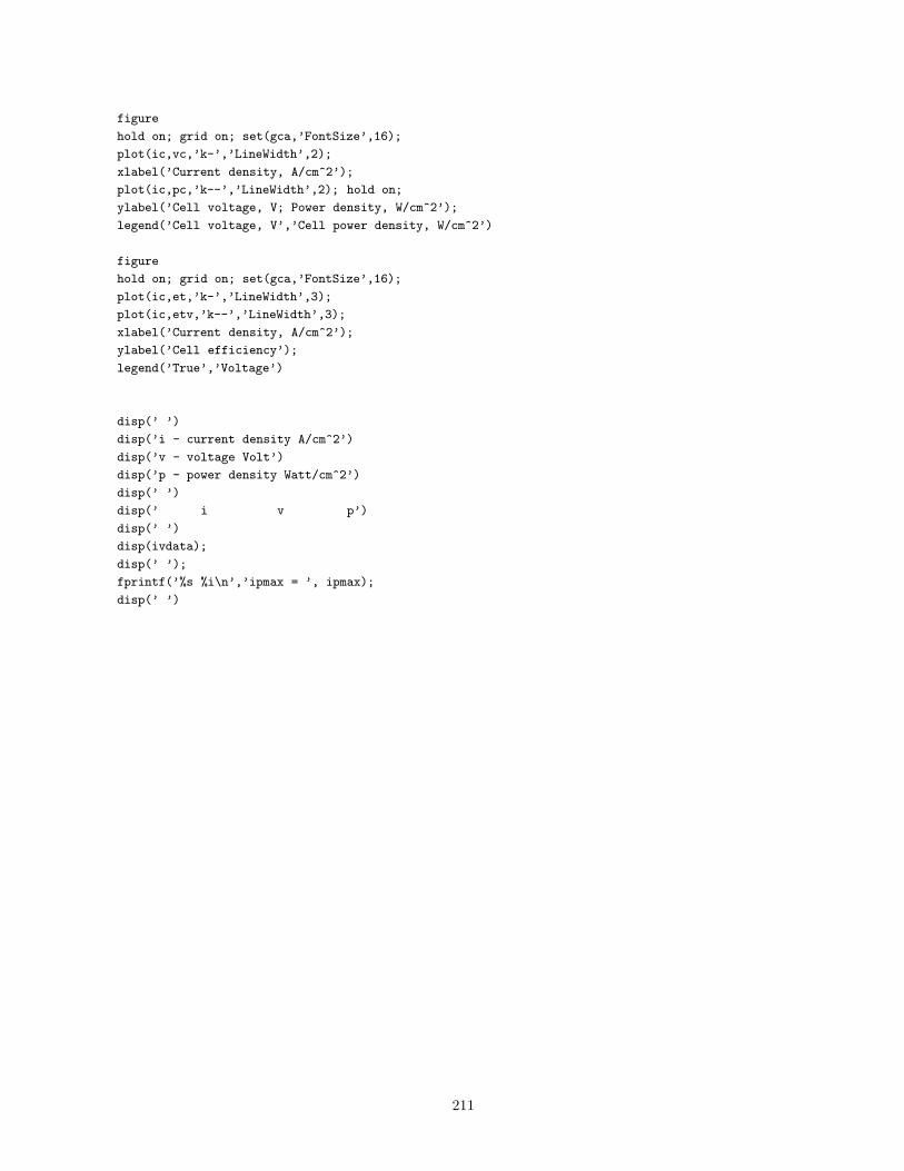
figure
hold on; grid on; set(gca,’FontSize’,16);
plot(ic,vc,’k-’,’LineWidth’,2);
xlabel(’Current density, A/cm^2’);
plot(ic,pc,’k--’,’LineWidth’,2); hold on;
ylabel(’Cell voltage, V; Power density, W/cm^2’);
legend(’Cell voltage, V’,’Cell power density, W/cm^2’)
figure
hold on; grid on; set(gca,’FontSize’,16);
plot(ic,et,’k-’,’LineWidth’,3);
plot(ic,etv,’k--’,’LineWidth’,3);
xlabel(’Current density, A/cm^2’);
ylabel(’Cell efficiency’);
legend(’True’,’Voltage’)
disp(’ ’)
disp(’i - current density A/cm^2’)
disp(’v - voltage Volt’)
disp(’p - power density Watt/cm^2’)
disp(’ ’)
disp(’ i v p’)
disp(’ ’)
disp(ivdata);
disp(’ ’);
fprintf(’%s %i\n’,’ipmax = ’, ipmax);
disp(’ ’)
211

% Driver for pemfc
% Size stack for an input gross power kW or vc or stack efficiency.
clear all
rundir = pwd;
srcdir = ’../src’;
fcvariables;
cd(srcdir)
pemfc;
cd(rundir);
212

% Driver for Design.
% Size stack for an input net power kWe or vc or stack efficiency.
clear all
rundir = pwd;
srcdir = ’../src’;
fcvariables;
cd(srcdir)
pemfcdesign;
cd(rundir);
213

% Driver for Analysis.
% For a fixed design, find operating space with altitude.
clear all
rundir = pwd;
srcdir = ’../src’;
fcvariables;
cd(srcdir)
% turn off plots
FCST.iplotVIP=0;
FCST.iprntSCR=1;
% design
pemfcdesign;
% Versus altitude
% First, Set operating current to design, max power, or max current
% (FCST.Istackdsg, FCST.IstackPmax, or FCST.Istackmax)
FCOP.Istack = FCST.Istackdsg;
% Now, vary altitude
Xrange = [0:500:14000]*0.3048;
FCOP.Istack = FCST.Istackdsg;
for iloop = 1:length(Xrange)
FCOP.altitude = Xrange(iloop);
pemfcstatic;
H1000ft(iloop) = FCOP.altitude/304.8;
pout(iloop) = FCOP.POWER_kW;
poute(iloop) = FCOP.POWER_kWe;
sfcout(iloop) = FCOP.SFC_kgkWhe;
H2SE(iloop) = 1/FCOP.SFC_kgkWhe;
H2in(iloop) = FCOP.MassH2rate_kgs;
end
cd(rundir);
FCOP.Pevs1000ft = [H1000ft; pout; poute; sfcout; H2in*3600];
% power vs altitude
figure;
hold on; grid on; set(gca,’FontSize’,16);
plot(H1000ft, pout,’k-’,’LineWidth’,3);
xlabel(’Altitude, x 1000 ft’); ylabel(’Gross Power,kW’);
figure;
hold on; grid on; set(gca,’FontSize’,16);
214

plot(H1000ft, poute,’k-’,’LineWidth’,3);
xlabel(’Altitude, x 1000 ft’); ylabel(’Net Power,kWe’);
% SFC vs altitude
figure;
hold on; grid on; set(gca,’FontSize’,16);
plot(H1000ft, sfcout,’k-’,’LineWidth’,3);
xlabel(’Altitude, x 1000 ft’); ylabel(’SFC,kg/kWhe’);
% fuel flow vs altitude
figure;
hold on; grid on; set(gca,’FontSize’,16);
plot(H1000ft, H2in*3600,’k-’,’LineWidth’,3);
xlabel(’Altitude, x 1000 ft’); ylabel(’H2 flow,kg/hr’);
215

% Driver for Analysis.
% For a fixed design, find operating space.
clear all
rundir = pwd;
srcdir = ’../src’;
fcvariables;
cd(srcdir)
% turn off plots
FCST.iplotVIP=0;
FCST.iprntSCR=1;
% design
FCST.POWERdsg_kW = 500;
pemfcdesign;
% Versus Current (i.e. fuel flow)
FCOP.iatm = 1;
FCOP.altitude = 5000*0.3048;
FCOP.temperatureC = 20;
% use a fraction of FCST.IstackPmax at higher altitude
Xrange = [100:100:1.0*FCST.IstackPmax];
for iloop = 1:length(Xrange)
FCOP.Istack = Xrange(iloop);
pemfcstatic;
vout(iloop) = FCOP.Vstack;
pout(iloop) = FCOP.POWER_kW;
sfcout(iloop) = FCOP.SFC_kgkWhe;
H2SE(iloop) = 1/FCOP.SFC_kgkWhe;
poute(iloop) = FCOP.POWER_kWe;
H2in(iloop) = FCOP.MassH2rate_kgs;
Airin(iloop) = FCOP.MassAirrate_kgs;
Waterliqout(iloop) = FCOP.MassWaterrate_kgs;
Watervapout(iloop) = FCOP.MassVaporrate_out_kgs;
Dryairout(iloop) = FCOP.MassAirrate_out_kgs - ...
FCOP.MassVaporrate_out_kgs;
end
cd(rundir);
FCOP.SFCvsPe = [poute; sfcout]; % kg/kWe-hr vs kWe
FCOP.SFCvsPefrac = [poute/FCST.POWERdsg_kWe; sfcout]; % kg/kWe-hr vs frac
FCOP.H2flowvsPe = [poute; H2in*3600]; % kg/hr vs kWe
% fuel flow vs net power
figure;
hold on; grid on; set(gca,’FontSize’,16);
plot(poute,H2in*3600,’k-’,’LineWidth’,3);
216

plot(poute,ones(1,length(poute))*FCST.MassH2rate_kgs*3600,...
’k-’,’LineWidth’,1);
xlabel(’Net Power, kWe’); ylabel(’H2 flow, kg/hr’);
% SFC vs net power and netpower/design power
figure;
hold on; grid on; set(gca,’FontSize’,16);
plot(poute,sfcout,’k-’,’LineWidth’,3);
plot(poute,ones(1,length(poute))*FCST.SFCPdsg_kgkWhe,...
’k-’,’LineWidth’,1);
xlabel(’Net Power, kWe’); ylabel(’SFC, kg/kWe-hr’);
figure;
hold on; grid on; set(gca,’FontSize’,16);
plot(poute/FCST.POWERdsg_kWe,sfcout,’k-’,’LineWidth’,3);
plot(poute/FCST.POWERdsg_kWe,ones(1,length(poute))*FCST.SFCPdsg_kgkWhe,...
’k-’,’LineWidth’,1);
xlabel(’Fraction of Net Design Power’); ylabel(’SFC, kg/kWe-hr’);
figure;
hold on; grid on; set(gca,’FontSize’,16);
plot(poute,H2SE,’k-’,’LineWidth’,3);
plot(poute,ones(1,length(poute))*(1/FCST.SFCPdsg_kgkWhe),...
’k-’,’LineWidth’,1);
xlabel(’Net Power, kWe’); ylabel(’Available Sp Energy, kWh/kg’);
title(’Available Specific Energy (1/SFC) vs Power’);
% Voltage and current vs net power
figure
hold on; grid on; set(gca,’FontSize’,16);
plot(poute,vout,’k-’,’LineWidth’,3);
plot(poute,pout,’r--’,’LineWidth’,3);
plot(poute,ones(1,length(poute))*FCST.Vstackdsg,...
’k-’,’LineWidth’,1);
plot(poute,ones(1,length(poute))*FCST.POWERdsg_kWe,...
’r-’,’LineWidth’,1);
legend(’Voltage’,’Current’);
xlabel(’Net Power, kWe’); ylabel(’Stack Voltage, V; Stack Current, A’);
title(’Voltage and Current vs Power’);
% Voltage and power vs current
figure
hold on; grid on; set(gca,’FontSize’,16);
plot(Xrange,vout,’k-’,’LineWidth’,3);
plot(Xrange,pout,’r--’,’LineWidth’,3);
plot(Xrange,poute,’r.-’,’LineWidth’,3);
plot(Xrange,ones(1,length(poute))*FCST.Vstackdsg,...
’k-’,’LineWidth’,1);
plot(Xrange,ones(1,length(poute))*FCST.POWERdsg_kWe,...
’r-’,’LineWidth’,1);
legend(’Voltage’,’Power’,’Power net’);
xlabel(’Stack current, A’); ylabel(’Stack Voltage, V; Stack Power, kW’);
title(’Voltage and Power vs Current’);
217

% Driver for Design.
% Design for fixed gross power kW (net power kWe + balance of plant).
% Vary power.
clear all
rundir = pwd;
srcdir = ’../src’;
fcvariables;
FCST.iplotVIP = 0;
vecPOWERdsg_kW = [50:50:600];
for iloopvecPOWERdsg_kW = 1:length(vecPOWERdsg_kW);
FCST.POWERdsg_kW = vecPOWERdsg_kW( iloopvecPOWERdsg_kW );
cd(srcdir)
pemfc;
cd(rundir);
Pout( iloopvecPOWERdsg_kW ) = FCST.POWERdsg_kW;
Poute( iloopvecPOWERdsg_kW ) = FCST.POWERdsg_kWe;
Poutmax( iloopvecPOWERdsg_kW ) = FCST.POWERmax_kW;
Poutmaxe( iloopvecPOWERdsg_kW ) = FCST.POWERmax_kWe;
Wout( iloopvecPOWERdsg_kW ) = FCST.Wtotal;
Wstacksysout( iloopvecPOWERdsg_kW ) = FCST.Wstacksys;
Wstackout( iloopvecPOWERdsg_kW ) = FCST.Wstack.total;
Wairout( iloopvecPOWERdsg_kW ) = FCST.Wair.total;
Wfuelout( iloopvecPOWERdsg_kW ) = FCST.Wfuel.H2;
Wtankout( iloopvecPOWERdsg_kW ) = FCST.Wfuel.tank;
Wltcout( iloopvecPOWERdsg_kW ) = FCST.Wlt.total;
Whtcout( iloopvecPOWERdsg_kW ) = FCST.Wht.total;
Wwaterout( iloopvecPOWERdsg_kW ) = FCST.Wwater.total;
Weleccout( iloopvecPOWERdsg_kW ) = FCST.Welec.total;
Wotherout( iloopvecPOWERdsg_kW ) = FCST.Wother;
Sout( iloopvecPOWERdsg_kW ) = FCST.Stotal;
Eout( iloopvecPOWERdsg_kW ) = FCST.EtadsgHHV;
end
FCST.StackWvsP = [Pout; Wstackout];
FCST.StackSystemWvsPe = [Poute; Poutmaxe; Wstacksysout];
% Stack weight vs gross design power
figure;
hold on; grid on; set(gca,’FontSize’,16);
plot(Wstackout,Pout,’k-’,’LineWidth’,3);
plot(Wstackout,Poutmax,’k--’,’LineWidth’,3);
legend(’Design’,’Maximum’);
xlabel(’Stack weight, kg’); ylabel(’Gross Power, kW’);
% Power-to-weight
218

figure;
hold on; grid on; set(gca,’FontSize’,16);
plot(Wstackout,Pout./Wstackout,’k-’,’LineWidth’,3);
xlabel(’Stack weight, kg’); ylabel(’Power/Weight, kW/kg’);
% Stack system weight vs net design power
figure;
hold on; grid on; set(gca,’FontSize’,16);
plot(Wstacksysout,Poute,’k-’,’LineWidth’,3);
plot(Wstacksysout,Poutmaxe,’k--’,’LineWidth’,3);
legend(’Design’,’Maximum’);
xlabel(’Stack system weight, kg’); ylabel(’Net Power, kWe’);
% Power-to-weight
figure;
hold on; grid on; set(gca,’FontSize’,16);
plot(Wstacksysout,Poute./Wstacksysout,’k-’,’LineWidth’,3);
xlabel(’Stack system Weight, kg’); ylabel(’Power/Weight, kWe/kg’);
% System weight break-down by components
figure;
hold on; grid on; set(gca,’FontSize’,16);
plot(Wout,Pout,’k-’,’LineWidth’,3);
plot(Wstackout,Pout,’k--’,’LineWidth’,3);
plot(Wairout,Pout,’r--’,’LineWidth’,2);
plot(Wltcout,Pout,’r--’,’LineWidth’,2);
plot(Whtcout,Pout,’r-’,’LineWidth’,2);
plot(Weleccout,Pout,’k-’,’LineWidth’,1);
plot(Wwaterout,Pout,’k--’,’LineWidth’,1);
ylabel(’Gross Power, kW’); xlabel(’Weight, kg’);
legend(’Total’,’Stack’,’Air’,’ltc’,’htc’,’elec’,’water’);
219

% Ragone plot
clear all
rundir = pwd;
srcdir = ’../src’;
fcvariables;
cd(srcdir)
FCST.iplotVIP = 0; % no performance plots
FCST.iprntSCR = 0; % no screen outputs
FCST.ioptf = 1; % fuel option 1
Fuelkg = 1:0.25:20;
for iloop=1:length(Fuelkg)
FCST.Whydrogen = Fuelkg(iloop);
pemfc;
% net @ design power
out10(iloop)= FCST.SEnergy_Pdsg_kWhekg;
out20(iloop)= FCST.SPower_Pdsg_kWekg;
out30(iloop)= FCST.EDensity_Pdsg_kWheL;
% net @ max power
out100(iloop)= FCST.SEnergy_Pmax_kWhekg;
out200(iloop)= FCST.SPower_Pmax_kWekg;
out300(iloop)= FCST.EDensity_Pmax_kWheL;
end
cd(rundir);
% net @ design power
figure
color = ’b-’;
x = out30*1e3; y = out20*1e3;
loglog(x,y,color,’LineWidth’,3); hold on; grid on; set(gca,’FontSize’,16);
xlabel(’Energy density, Whe/L’); ylabel(’Specific power, We/kg’);
title(’@ Design Power’)
axis([50 1000 50 5000])
figure
x = out10*1e3; y = out20*1e3;
loglog(x,y,color,’LineWidth’,3); hold on; grid on; set(gca,’FontSize’,16);
xlabel(’Specific energy, Whe/kg’); ylabel(’Specific power, We/kg’);
title(’@ Design Power’)
axis([50 1000 50 5000])
clear x;
x=[1 1000];
y=x./(4.0); loglog(x,y,’k--’,’LineWidth’,2); % 4 hr line
y=x./(2.0); loglog(x,y,’k--’,’LineWidth’,2); % 2 hr line
y=x./(1.0); loglog(x,y,’k--’,’LineWidth’,2); % 1 hr line
220

y=x./(0.5); loglog(x,y,’k--’,’LineWidth’,2); % 30 min
y=x./(0.25); loglog(x,y,’k--’,’LineWidth’,2); % 15 min
y=x./(0.125); loglog(x,y,’k--’,’LineWidth’,2); % 7.5 min
h=text(700,200,’ 4 hours’); set(h,’Rotation’,30,’FontSize’,14);
h=text(700,400,’ 2 hours’); set(h,’Rotation’,30,’FontSize’,14);
h=text(700,800,’ 1 hour’); set(h,’Rotation’,30,’FontSize’,14);
h=text(700,1600,’30 mins’); set(h,’Rotation’,30,’FontSize’,14);
h=text(600,2600,’15 mins’); set(h,’Rotation’,30,’FontSize’,14);
h=text(300,2600,’7.5 mins’); set(h,’Rotation’,30,’FontSize’,14);
% net @ max power
color = ’r-’;
figure
x = out300*1e3; y = out200*1e3;
loglog(x,y,color,’LineWidth’,3); hold on; grid on; set(gca,’FontSize’,16);
xlabel(’Energy density, Whe/L’); ylabel(’Specific power, We/kg’);
title(’@ Max Power’)
axis([50 1000 50 2000])
figure
x = out100*1e3; y = out200*1e3;
loglog(x,y,color,’LineWidth’,3); hold on; grid on; set(gca,’FontSize’,16);
xlabel(’Specific energy, Whe/kg’); ylabel(’Specific power, We/kg’);
title(’@ Max Power’)
axis([50 1000 50 5000])
clear x;
x=[1 1000];
y=x./(4.0); loglog(x,y,’k--’,’LineWidth’,2); % 4 hr line
y=x./(2.0); loglog(x,y,’k--’,’LineWidth’,2); % 2 hr line
y=x./(1.0); loglog(x,y,’k--’,’LineWidth’,2); % 1 hr line
y=x./(0.5); loglog(x,y,’k--’,’LineWidth’,2); % 30 min
y=x./(0.25); loglog(x,y,’k--’,’LineWidth’,2); % 15 min
y=x./(0.125); loglog(x,y,’k--’,’LineWidth’,2); % 7.5 min
h=text(700,200,’ 4 hours’); set(h,’Rotation’,30,’FontSize’,14);
h=text(700,400,’ 2 hours’); set(h,’Rotation’,30,’FontSize’,14);
h=text(700,800,’ 1 hour’); set(h,’Rotation’,30,’FontSize’,14);
h=text(700,1600,’30 mins’); set(h,’Rotation’,30,’FontSize’,14);
h=text(600,2600,’15 mins’); set(h,’Rotation’,30,’FontSize’,14);
h=text(300,2600,’7.5 mins’); set(h,’Rotation’,30,’FontSize’,14);
221

% Driver for Design.
% Design for fixed net power kWe (gross power kW - balance of plant).
% Vary altitude.
clear all
rundir = pwd;
srcdir = ’../src’;
fcvariables;
FCST.iplotVIP = 0;
kWe = 80;
vecaltitudeDesign = [0:1000:14000]*0.3048; % m
for iloopvec = 1:length(vecaltitudeDesign);
FCST.altitudeDesign = vecaltitudeDesign( iloopvec );
FCST.POWERdsg_kW = kWe;
cd(srcdir)
pemfcdesign; close all;
cd(rundir);
H1000ft( iloopvec ) = FCST.altitudeDesign/304.8;
Pout( iloopvec ) = FCST.POWERdsg_kW;
Poute( iloopvec ) = FCST.POWERdsg_kWe;
Wout( iloopvec ) = FCST.Wtotal;
Wstackout( iloopvec ) = FCST.Wstack.total;
Wairout( iloopvec ) = FCST.Wair.total;
Wfuelout( iloopvec ) = FCST.Wfuel.H2;
Wtankout( iloopvec ) = FCST.Wfuel.tank;
Wltcout( iloopvec ) = FCST.Wlt.total;
Whtcout( iloopvec ) = FCST.Wht.total;
Wwaterout( iloopvec ) = FCST.Wwater.total;
Weleccout( iloopvec ) = FCST.Welec.total;
Wotherout( iloopvec ) = FCST.Wother;
Sout( iloopvec ) = FCST.Stotal;
Eout( iloopvec ) = FCST.EtadsgHHV;
end
W = Wout - Wfuelout - Wtankout;
FCST.StackSystemWvsH = [vecaltitudeDesign; W];
% altitude vs Stack weight
figure;
hold on; grid on; set(gca,’FontSize’,16);
plot(Wstackout,H1000ft,’k-’,’LineWidth’,3);
ylabel(’Altitude, x 1000 ft’); xlabel(’Stack weight, kg’);
222

% altitude vs Stack system weight
figure;
hold on; grid on; set(gca,’FontSize’,16);
plot(W,H1000ft,’k-’,’LineWidth’,3);
ylabel(’Altitude, x 1000 ft’); xlabel(’Stack system weight, kg’);
% weight break-down by components
figure;
hold on; grid on; set(gca,’FontSize’,16);
plot(W,H1000ft,’k-’,’LineWidth’,3);
plot(Wstackout,H1000ft,’k--’,’LineWidth’,3);
plot(Wairout,H1000ft,’b--’,’LineWidth’,2);
plot(Wltcout,H1000ft,’r--’,’LineWidth’,2);
plot(Whtcout,H1000ft,’r-’,’LineWidth’,2);
plot(Weleccout,H1000ft,’k-’,’LineWidth’,1);
plot(Wwaterout,H1000ft,’k--’,’LineWidth’,1);
ylabel(’Altitude, x 1000 ft’); xlabel(’Weight, kg’);
legend(’Total’,’Stack’,’Air’,’ltc’,’htc’,’elec’,’water’);
223

The input decks fcvariables.m.
Only the inputs for run Baseline 80kW, run Modern 80 kW, and run Modern 80 kW liqcool are listed. The others
need small changes that are described in the report.
224
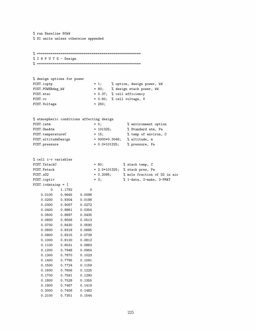
% run Baseline 80kW
% SI units unless otherwise appended
% =====================================================
% I N P U T S - Design
% =====================================================
% design options for power
FCST.ioptp = 1; % option, design power, kW
FCST.POWERdsg_kW = 80; % design stack power, kW
FCST.etac = 0.37; % cell efficiency
FCST.vc = 0.60; % cell voltage, V
FCST.Voltage = 250;
% atmospheric conditions affecting design
FCST.iatm = 0; % environment option
FCST.OneAtm = 101325; % Standard atm, Pa
FCST.temperatureC = 15; % temp of environ, C
FCST.altitudeDesign = 0000*0.3048; % altitude, m
FCST.pressure = 0.0*101325; % pressure, Pa
% cell i-v variables
FCST.TstackC = 80; % stack temp, C
FCST.Pstack = 2.5*101325; % stack pres, Pa
FCST.xO2 = 0.2095; % mole fraction of O2 in air
FCST.ioptiv = 3; % 1-data, 2-make, 3-PMAT
FCST.ivdatainp = [
0 1.1782 0
0.0100 0.9645 0.0096
0.0200 0.9304 0.0186
0.0300 0.9057 0.0272
0.0400 0.8861 0.0354
0.0500 0.8697 0.0435
0.0600 0.8556 0.0513
0.0700 0.8430 0.0590
0.0800 0.8318 0.0665
0.0900 0.8215 0.0739
0.1000 0.8120 0.0812
0.1100 0.8031 0.0883
0.1200 0.7948 0.0954
0.1300 0.7870 0.1023
0.1400 0.7795 0.1091
0.1500 0.7724 0.1159
0.1600 0.7656 0.1225
0.1700 0.7591 0.1290
0.1800 0.7528 0.1355
0.1900 0.7467 0.1419
0.2000 0.7408 0.1482
0.2100 0.7351 0.1544
225

0.2200 0.7295 0.1605
0.2300 0.7241 0.1665
0.2400 0.7187 0.1725
0.2500 0.7135 0.1784
0.2600 0.7084 0.1842
0.2700 0.7035 0.1899
0.2800 0.6985 0.1956
0.2900 0.6937 0.2012
0.3000 0.6890 0.2067
0.3100 0.6843 0.2121
0.3200 0.6796 0.2175
0.3300 0.6751 0.2228
0.3400 0.6706 0.2280
0.3500 0.6661 0.2331
0.3600 0.6617 0.2382
0.3700 0.6573 0.2432
0.3800 0.6529 0.2481
0.3900 0.6486 0.2530
0.4000 0.6444 0.2577
0.4100 0.6401 0.2624
0.4200 0.6359 0.2671
0.4300 0.6317 0.2716
0.4400 0.6275 0.2761
0.4500 0.6233 0.2805
0.4600 0.6192 0.2848
0.4700 0.6150 0.2891
0.4800 0.6109 0.2932
0.4900 0.6068 0.2973
0.5000 0.6027 0.3013
0.5100 0.5985 0.3053
0.5200 0.5944 0.3091
0.5300 0.5903 0.3129
0.5400 0.5862 0.3165
0.5500 0.5821 0.3201
0.5600 0.5779 0.3236
0.5700 0.5738 0.3271
0.5800 0.5696 0.3304
0.5900 0.5655 0.3336
0.6000 0.5613 0.3368
0.6100 0.5571 0.3398
0.6200 0.5529 0.3428
0.6300 0.5486 0.3456
0.6400 0.5443 0.3484
0.6500 0.5400 0.3510
0.6600 0.5357 0.3535
0.6700 0.5313 0.3559
0.6800 0.5268 0.3582
0.6900 0.5224 0.3604
0.7000 0.5178 0.3625
0.7100 0.5133 0.3644
0.7200 0.5086 0.3662
0.7300 0.5039 0.3679
0.7400 0.4992 0.3694
226

0.7500 0.4943 0.3707
0.7600 0.4894 0.3720
0.7700 0.4844 0.3730
0.7800 0.4793 0.3738
0.7900 0.4741 0.3745
0.8000 0.4687 0.3750
0.8100 0.4633 0.3753
0.8200 0.4577 0.3753
0.8300 0.4520 0.3751
0.8400 0.4460 0.3747
0.8500 0.4399 0.3739
0.8600 0.4336 0.3729
0.8700 0.4270 0.3715
0.8800 0.4202 0.3698
0.8900 0.4131 0.3677
0.9000 0.4056 0.3651
0.9100 0.3978 0.3620
0.9200 0.3894 0.3583
0.9300 0.3805 0.3539
0.9400 0.3710 0.3487
0.9500 0.3606 0.3426
0.9600 0.3493 0.3354
0.9700 0.3368 0.3267
0.9800 0.3225 0.3161
0.9900 0.3061 0.3030
1.0000 0.2864 0.2864
1.0100 0.2615 0.2641
1.0200 0.2272 0.2317
1.0300 0.1699 0.1750
];
FCST.ipmaxinp = 83;
FCST.Er = 1.1782;
FCST.j0C = 0.0001;
FCST.alphaC = 0.155;
FCST.j0A = 0.1;
FCST.alphaA = 0.5;
FCST.ASR = 0.1075;
FCST.jL = 1.05;
FCST.jleak = 0.01;
FCST.C = 0.08;
FCST.PMAT = [
1 2 3 4 % Presssure, atm
0.0001 0.0001 0.0001 0.0001 % jOC
0.1500 0.1550 0.1550 0.1600 % alphaC
0.1000 0.1000 0.1000 0.1000 % jOA
0.5000 0.5000 0.5000 0.5000 % alphaA
0.1200 0.1150 0.1000 0.0600 % ASR, Ohm cm2
0.7300 1.0000 1.1000 1.2300 % jL, A/cm2
0.0100 0.0100 0.0100 0.0100 % jLeak, A/cm2
0.0800 0.0800 0.0800 0.1200 % C, Volt
];
FCST.crh = 100;
FCST.arh = 100;
227

FCST.deltai = 0.02;
% temp corr
FCST.ASR0 = 0.12; % ref value
FCST.ASR0t = 80; % ref temp
FCST.ASRtk2 = 0.0006;
FCST.ASRtk1 = 0.002;
FCST.jL0 = 0.73; % ref value
FCST.jL0t = 80; % ref temp
FCST.jLtk2 = -0.0015;
FCST.jLtk1 = -0.003;
% humidity corrections in ASR and jL
FCST.ASR0arh = 100; % ref anode rh
FCST.ASR0crh = 100; % ref cathode rh
FCST.ASRrhk1a = -0.005;
FCST.ASRrhk2a = 0.;
FCST.ASRrhk1a1c = 0.;
FCST.ASRrhk1a2c = 2.0e-6;
FCST.ASRrhk2a2c = 0.;
FCST.ASRrhk2a1c = 0.;
FCST.ASRrhk2c = 7.0e-5;
FCST.ASRrhk1c = 0.0021;
FCST.jL0arh = 100;
FCST.jL0crh = 100;
FCST.jLrhk1a = 0.;
FCST.jLrhk2a = 0.;
FCST.jLrhk1a1c = 0.;
FCST.jLrhk1a2c = 0.;
FCST.jLrhk2a2c = 0.;
FCST.jLrhk2a1c = 0.;
FCST.jLrhk2c = -0.0001;
FCST.jLrhk1c = -0.0076;
% other corrections
FCST.icorr = 0; % ic corr (0/1)
FCST.TFi = 1.0; % changes ic to ic.Tfi
FCST.vcorr = 0; % vc corr for alt (0/1)
FCST.deltav = -0.01; % cell to stack correction
FCST.vrate1000ft = -0.0056; % percent drop / 1000 ft
FCST.vdropaboveft = 1000; % above 1000-ft
% stack weight variables
FCST.TFwstack = 1.0; % Tech factor stack weight
FCST.dWwstack = 0.0; % correction stack weight
FCST.TFsstack = 1.0; % Tech factor stack volume
FCST.dSsstack = 0.0; % correction stack volume
FCST.ioptsw = 1; % 0: simple, 1: detailed
FCST.tcell = 0.001381; % cell thickness, m
FCST.dcell = 2584; % cell density, kg/m3
FCST.porosity = 1.0;
% Component breakdown
FCST.dendplate = 1600; % end plate, Al
FCST.dinsulplate = 1420; % polyoxy-methylene
FCST.dcollplate = 8940; % collector plate, Cu
228

FCST.dpem = 500; % membrane, Nafion
FCST.dgdl = 440; % gas diffusion layer
FCST.dbipolarplate = 2160; % graphite
FCST.dgasket = 1000; % rubber
FCST.Aendplatefrac = 1.1; % Area = 1.1 Active area
FCST.tendplatecons = 0.0; % thickness constant
FCST.tendplatefrac = 0.020; % thickness = 0.05 tunit
FCST.Ainsulplatefrac = 1.1; % fraction active area
FCST.tinsulplatecons = 0.0; % thickness constrant
FCST.tinsulplatefrac = 0.005; % thickness = 0.02 tunit
FCST.Acollplatefrac = 0.5; % fraction active area
FCST.tcollplatecons = 0.0; % thickness constant
FCST.tcollplatefrac = 0.005; % thickness = 0.01 tunit
FCST.Wfastener = 0.0; % bolt/clamp, steel, 7850 kg/m3
FCST.tpem = 0.00010; % membrane, Nafion
FCST.tgdl = 0.00020; % gas diffusion layer
FCST.tbipolarplate = 0.00100; % graphite; avg seal + mea region
FCST.pbipolarplate = 0.60000; % porosity due to channels
FCST.Abipolarplatefrac = 1.10; % fraction active area
FCST.tgasket = 0.00200; % rubber
FCST.Agasketfrac = 0.03; % fraction active area
FCST.Wstackother = 0.00; % any other weight
% H2 tank system
FCST.fH2utilization = 1.0;
FCST.itanktype = 3;
FCST.ioptf = 1; % fuel option; 1-h2, 2-endurance
FCST.Whydrogen = 5;
FCST.Endurance_min = 60;
% 350 bar: 0.0515, 17.2; 700 bar: 0.057, 40;
% cryo-compressed Al: 0.09, 41; cryo-compressed steel: 0.055, 41
% liq: 0.075, 65;
FCST.h2tankwfg = 0.057; % kg/kg wt fraction gravimetric
FCST.h2tankwfs = 40.00; % kg/m3 wt fraction volumetric
FCST.h2tankBar = 700; % tank storage pressure
FCST.h2tankTC = 15; % tank storage temperature C
FCST.h2tankSov = 0.10; % tank volume overhead
FCST.FuelFilterW0 = 0.;
FCST.FuelFilterfW = 0.;
FCST.FuelRegulatorW0 = 0; % kg
FCST.FuelRegulatorfW = 0.01; % fraction fuel sys wt
FCST.FuelPowerW0 = 0; % kg wt of power supply
FCST.FuelPowerfW = 0.01; % fraction fuel sys wt
FCST.FuelPlumbW0 = 0; % kg plumbing constant wt
FCST.FuelPlumbWw = 0; % kg/m plumb wt per length
FCST.FuelPlumbWl = 0; % m plumb length
FCST.Pfuel0 = 0; % prescribed power
FCST.Pfuelk = 0; % prop to fuel flow rate
FCST.Pfuele = 0; % expo to fuel flow rate
FCST.FGErho = 722.13;% density of gasoline
229

FCST.FGEMJkg = 44; % heating value of gasoline, MJ/kg
FCST.FGEeta = 0.25; % efficiency of FGE fuel
% Air system variables
FCST.fAirFlowRate = 2.5;
FCST.DPstack = 30000; % pres drop in stack, Pa
% Blower
FCST.iBlower = 0;
FCST.BlowEta = 0.75;
FCST.BlowW0 = 0;
FCST.BlowWtf = 1.0;
FCST.BlowWk = 1/1000;
FCST.BlowWfe = 0;
FCST.BlowWpe = 1;
FCST.BlowS0 = 0;
FCST.BlowStf = 1.0;
FCST.BlowSk = 1/3e6;
FCST.BlowSfe = 0;
FCST.BlowSpe = 1;
% Compressor
FCST.iCompressor = 1;
FCST.CompEta = 0.75;
FCST.CompW0 = 0.;
FCST.CompWtf = 1.0;
FCST.CompWk = 7e-4; % 122 kg/kg/s or 7e-4 kg/W
FCST.CompWfe = 0;
FCST.CompWpe = 1;
FCST.CompS0 = 0.;
FCST.CompStf = 1.0;
FCST.CompSk = 4.14e-7; % 0.0722 m3/kg/s or 4.14e-7 m3/W
FCST.CompSfe = 0;
FCST.CompSpe = 1;
% Turbo-expander (axial-flow turbine)
FCST.iTurbine = 1;
FCST.TurbEta = 0.75;
FCST.TurbW0 = 0.;
FCST.TurbWtf = 1.0;
FCST.TurbWk = 0;
FCST.TurbWfe = 0;
FCST.TurbWpe = 0;
FCST.TurbS0 = 0.;
FCST.TurbStf = 1.0;
FCST.TurbSk = 0;
FCST.TurbSfe = 0;
FCST.TurbSpe = 0;
% accessories
FCST.AirFilterW0 = 0; % kg
FCST.AirFilterfW = 0.01; % fraction Air sys wt
FCST.AirRegulatorW0 = 0; % kg
230

FCST.AirRegulatorfW = 0.01; % fraction Air sys wt
FCST.AirPowerW0 = 0; % kg controller
FCST.AirPowerfW = 0.05; % fraction Air sys wt
FCST.AirPlumbW0 = 0; % kg plumbing constant wt
FCST.AirPlumbWw = 0; % kg/m plumb wt per length
FCST.AirPlumbWl = 0; % m plumb length
FCST.AirHumidifierW0 = 0; % kg
FCST.AirHumidifierfW = 0.05; % fraction Air sys wt
% Heat system variables
% low temp system (air pre-cooler, only if compressor used)
FCST.iLTR = 0; % 0-Pdsg load, 1-Pmax load
FCST.ltRadiatorhr = 1015; % rad conv ht trans coeff W/m2/K
FCST.ltRadiatorTa = 20; % rad Ta in C
FCST.ltRadiatorTr = 95; % rad Tr in C
FCST.ltRadiatorepr = 0.8; % rad emissivity
FCST.ltRadiatorW0 = 0; % kg
FCST.ltRadiatorWk = 1e-4; % kg/W (f=0) 1e-4 or kg/m2 (e=0) 3.5405
FCST.ltRadiatorWe = 1;
FCST.ltRadiatorWf = 0;
FCST.ltRadiatorS0 = 0; % m3
FCST.ltRadiatorSk = 1e-7; % m3/W (f=0) 1e-7 or thick (e=0) 0.035
FCST.ltRadiatorSe = 1;
FCST.ltRadiatorSf = 0;
FCST.ltCoolantCp = 4180; % J/kg-K (water)
FCST.ltCoolantdT = 10; % coolant deltaT (max 15)
FCST.ltCoolantW0 = 0; % kg
FCST.ltCoolantWk = 1e-6; % kg/W (f=0) 1e-6 or time sec (e=0) 30
FCST.ltCoolantWe = 1;
FCST.ltCoolantWf = 0;
FCST.ltCoolerW0 = 0; % kg
FCST.ltCoolerWk = 1e-6; % kg/W
FCST.ltCoolerWe = 1; %
FCST.ltFilterW0 = 0; % kg
FCST.ltFilterfW = 0.01; % fraction Heat sys wt
FCST.ltRegulatorW0 = 0; % kg
FCST.ltRegulatorfW = 0.01; % fraction Heat sys wt
FCST.ltPowerW0 = 0; % kg
FCST.ltPowerfW = 0.01; % fraction Heat sys wt
FCST.ltPlumbW0 = 0; % kg plumbing constant wt
FCST.ltPlumbWw = 0; % kg/m plumb wt per length
FCST.ltPlumbWl = 0; % m plumb length
FCST.Plt0 = 0; % any power needed
FCST.Pltk = 0.01; % 0.01-heat, kPa-flow (water)
FCST.Plte = 1; % expo to heating
FCST.Pltf = 0; % expo to flow
% Heat system variables
% high temp system (stack cooling)
FCST.iHV = 0; % 0-LHV, 1-HHV
231

FCST.iHTR = 0; % 0-Pdsg load, 1-Pmax load
FCST.htStackfd = 0; % stack frac stack heat dissipated
FCST.htStackhs = 3; % stack conv ht trans coeff W/m2/K
FCST.htStackTa = 40; % stack Ta in C
FCST.htStackeps = 0.8; % stack emissivity
FCST.htStackfs = 0.6; % stack frac surface/active area
FCST.htRadiatorhr = 1015; % rad conv ht trans coeff W/m2/K
FCST.htRadiatorTa = 20; % rad Ta in C
FCST.htRadiatorTr = 95; % rad Tr in C
FCST.htRadiatorepr = 0.8; % rad emissivity
FCST.htRadiatorW0 = 0; % kg
FCST.htRadiatorWk = 1e-5; % kg/W (f=0) 1e-5 or kg/m2 (e=0) 3.5405
FCST.htRadiatorWe = 1;
FCST.htRadiatorWf = 0;
FCST.htRadiatorS0 = 0; % m3
FCST.htRadiatorSk = 1e-7; % m3/W (f=0) 1e-7 or thick (e=0) 0.035
FCST.htRadiatorSe = 1;
FCST.htRadiatorSf = 0;
FCST.htCoolantCp = 4180; % J/kg-K (water)
FCST.htCoolantrho = 997; % kg/m3 (water)
FCST.htCoolantdT = 10; % coolant Tc in C
FCST.htCoolantW0 = 0; % kg
FCST.htCoolantWk = 1e-6; % kg/W (f=0) 1e-6 or time sec (e=0) 5
FCST.htCoolantWe = 1;
FCST.htCoolantWf = 0;
FCST.htFilterW0 = 0; % kg
FCST.htFilterfW = 0.01; % fraction Heat sys wt
FCST.htRegulatorW0 = 0; % kg
FCST.htRegulatorfW = 0.01; % fraction Heat sys wt
FCST.htPowerW0 = 0; % kg
FCST.htPowerfW = 0.01; % fraction Heat sys wt
FCST.htPlumbW0 = 0; % kg plumbing constant wt
FCST.htPlumbWw = 0; % kg/m plumb wt per length
FCST.htPlumbWl = 0; % m plumb length
FCST.Pht0 = 0; % any power needed
FCST.Phtk = 0.01; % 0.01-heat, kPa-flow (water)
FCST.Phte = 1; % expo to heat
FCST.Phtf = 0; % expo to coolant flow
% Water system variables
FCST.rhowater = 997; % kg/m3
FCST.waterstoragefrac = 0.2; % fraction of produce stored
FCST.waterstoragehour = 0.5; % accumulated over this time
FCST.watertankSov = 0; % Stank = (1+Sov).Swater
FCST.watertankWov = 0; % Wtank = (1+Wov).Wwater
FCST.waterFilterW0 = 0; % kg
FCST.waterFilterfW = 0; % fraction Heat sys wt
FCST.waterRegulatorW0 = 0; % kg
FCST.waterRegulatorfW = 0; % fraction water sys wt
FCST.waterPowerW0 = 0; % kg
FCST.waterPowerfW = 0; % fraction water sys wt
FCST.waterPlumbW0 = 0; % kg plumbing constant wt
232

FCST.waterPlumbWw = 0; % kg/m plumb wt per length
FCST.waterPlumbWl = 0; % m plumb length
FCST.Pwater0 = 0; % any power needed
FCST.Pwaterk = 1e6; % prop to liq water flow
FCST.Pwatere = 1; % expo to liq water flow
% electrical system variables
FCST.elecControlW0 = 0; % kg
FCST.elecControlWk = 0.01; % prop to stack current
FCST.elecControlWe = 1.0; % expo to stack current
FCST.elecRegulatorW0 = 0; % kg
FCST.elecRegulatorfW = 0; % fraction elec sys wt
FCST.elecPowerW0 = 0; % kg
FCST.elecPowerfW = 0.01; % fraction elec sys wt
FCST.elecPlumbW0 = 0; % kg plumbing constant wt
FCST.elecPlumbWwk = 0.01; % prop to stack current
FCST.elecPlumbWwe = 1.0; % expo to stack current
FCST.elecPlumbWl = 0; % m plumb length
FCST.Pelec0 = 0; % any power needed
FCST.Peleck = 0.02; % prop to stack power
FCST.Pelece = 1.0; % expo to stack power
% additional gross overhead fractions
FCST.fovpower = 0.0;
FCST.fovweight = 0.0;
FCST.fovvolume = 0.0;
% output options
FCST.iplotVIP = 1;
FCST.iprntSCR = 1;
% =====================================================
% O U T P U T S - Design
% =====================================================
% overall weight, power, energy, and specific quantities
% stack efficiencies
FCST.etadsgHHV = 0.;
FCST.etadsgLHV = 0.;
FCST.etamaxHHV = 0.;
FCST.etamaxLHV = 0.;
% net system efficiencies
FCST.EtadsgHHV = 0.;
FCST.EtadsgLHV = 0.;
FCST.EtamaxHHV = 0.;
FCST.EtamaxLHV = 0.;
233

% Fuel gallon equivalents
FCST.FGEHHV = 0.; % chemical
FCST.FGELHV = 0.; % chemical
FCST.FGEHHVtrue = 0.; % engine (chemical x efficiency)
FCST.FGELHVtrue = 0.; % engine (chemical x efficiency)
FCST.Wtotal = 0.;
FCST.Stotal = 0.;
FCST.Wstacksys = 0.;
FCST.Sstacksys = 0.;
FCST.DFstacksys = 0.;
FCST.SFCPdsg_kgkWh = 0.;
FCST.SFCPmax_kgkWh = 0.;
FCST.SFCPdsg_kgkWhe = 0.;
FCST.SFCPmax_kgkWhe = 0.;
FCST.POWERdsg_kWe = 0.;
FCST.POWERmax_kW = 0.;
FCST.POWERmax_kWe = 0.;
FCST.ENERGY_Pdsg_kWh = 0.;
FCST.ENERGY_Pdsg_kWhe = 0.;
FCST.ENERGY_Pmax_kWh = 0.;
FCST.ENERGY_Pmax_kWhe = 0.;
FCST.SPower_Pdsg_Stack_kWkg = 0.;
FCST.SPower_Pdsg_Stack_kWekg = 0.;
FCST.SPower_Pmax_Stack_kWkg = 0.;
FCST.SPower_Pmax_Stack_kWekg = 0.;
FCST.SPower_Pdsg_Stacksys_kWkg = 0.;
FCST.SPower_Pdsg_Stacksys_kWekg= 0.;
FCST.SPower_Pmax_Stacksys_kWkg = 0.;
FCST.SPower_Pmax_Stacksys_kWekg= 0.;
FCST.SPower_Pdsg_kWkg = 0.;
FCST.SPower_Pdsg_kWekg = 0.;
FCST.SPower_Pmax_kWkg = 0.;
FCST.SPower_Pmax_kWekg = 0.;
FCST.EDensity_Pdsg_kWhL = 0.;
FCST.EDensity_Pdsg_kWheL = 0.;
FCST.EDensity_Pmax_kWhL = 0.;
FCST.EDensity_Pmax_kWheL = 0.;
FCST.SEnergy_Pdsg_kWhkg = 0.;
FCST.SEnergy_Pdsg_kWhekg = 0.;
FCST.SEnergy_Pmax_kWhkg = 0.;
FCST.SEnergy_Pmax_kWhekg = 0.;
% stack variables
% performance
FCST.ivdata = 0.;
FCST.Eh = 0.;
234

FCST.Er = 0.;
FCST.Aactive_cm2 = 0.;
FCST.Ncell = 0.;
FCST.Istackdsg = 0.;
FCST.Vstackdsg = 0.;
FCST.Istackmax = 0.;
FCST.Vstackmax = 0.;
FCST.IstackPmax = 0.;
FCST.VstackPmax = 0.;
FCST.SP = 0.;
FCST.SPmax = 0.;
FCST.vcdsg = 0.;
FCST.icdsg = 0.;
FCST.pcdsg = 0.;
FCST.etavdsgHHV = 0.;
FCST.etavdsgLHV = 0.;
% size
FCST.Sstack = 0.;
FCST.Lstack = 0.;
FCST.Astack = 0.;
FCST.DFstack = 0.;
Wstack.total = 0.;
Wstack.endplate = 0.;
Wstack.insulplate = 0.;
Wstack.collplate = 0.;
Wstack.unit = 0.;
Wstack.cell = 0.;
Wstack.mea = 0.;
Wstack.bipolarplate = 0.;
Wstack.pem = 0.;
Wstack.gdl = 0.;
Wstack.gasket = 0.;
Wstack.other = 0.;
FCST.Wstack = Wstack;
FCST.Wstackk0 = 0.;
FCST.Wstackk1 = 0.;
% Air system variables
FCST.Sblower = 0.;
FCST.Scomp = 0.;
FCST.Sturb = 0.;
Wair.total = 0.;
Wair.blower = 0.;
Wair.comp = 0.;
Wair.turb = 0.;
Wair.precooler = 0.;
Wair.humidifier = 0.;
Wair.filter = 0.;
Wair.plumbing = 0.;
Wair.power = 0.;
235

Wair.regulator = 0.;
FCST.Wair = Wair;
FCST.Pair_kW = 0.;
FCST.Pairmax_kW = 0.;
FCST.Pblower_kW = 0.;
FCST.Pblowermax_kW = 0.;
FCST.Pcomp_kW = 0.;
FCST.Pcompmax_kW = 0.;
FCST.Pturb_kW = 0.;
FCST.Pturbmax_kW = 0.;
FCST.MassAirrate_kgs = 0.;
FCST.MassAirrate_max_kgs = 0.;
FCST.MassAirrate_Ls = 0.;
FCST.MassAirrate_max_Ls = 0.;
FCST.MassAirrate_out_kgs = 0.;
FCST.MassAirrate_out_max_kgs = 0.;
FCST.Humidity_ratio = 0.;
FCST.MassWaterrate_kgs = 0.;
FCST.MassVaporrate_kgs = 0.;
FCST.MassLiquidrate_kgs = 0.;
% Fuel system variables
FCST.Sh2tank = 0.;
Wfuel.total = 0.;
Wfuel.H2 = 0.;
Wfuel.tank = 0.;
Wfuel.filter = 0.;
Wfuel.plumbing = 0.;
Wfuel.power = 0.;
Wfuel.regulator = 0.;
FCST.Wfuel = Wfuel;
FCST.Pfuel_kW = 0.;
FCST.Pfuelmax_kW = 0.;
FCST.MassH2rate_kgs = 0.;
FCST.MassH2rate_Pmax_kgs = 0.;
FCST.SFCPdsg_kgkWh = 0.;
FCST.SFCPmax_kgkWh = 0.;
% low temp cooling system variables (air pre-cooler)
Wlt.total = 0.;
Wlt.filter = 0.;
Wlt.plumbing = 0.;
Wlt.regulator = 0.;
Wlt.coolant = 0.;
Wlt.radiator = 0.;
Wlt.power = 0.;
FCST.Wlt = Wlt;
FCST.Plt_kW = 0.;
FCST.Pltmax_kW = 0.;
FCST.Sltradiator = 0.;
236

FCST.Altradiator = 0.;
FCST.HEATINGlt_kW = 0.;
FCST.HEATINGlt_max_kW = 0.;
FCST.Cflowmaxlt = 0.;
FCST.Cflowdsglt = 0.;
FCST.Cflowlt = 0.;
% high temp cooling system variables (stack cooler)
Wht.total = 0.;
Wht.filter = 0.;
Wht.plumbing = 0.;
Wht.regulator = 0.;
Wht.coolant = 0.;
Wht.radiator = 0.;
Wht.power = 0.;
FCST.Wht = Wht;
FCST.Pht_kW = 0.;
FCST.Phtmax_kW = 0.;
FCST.Shtradiator = 0.;
FCST.Ahtradiator = 0.;
FCST.HEATINGstack_kW = 0.;
FCST.HEATINGairin_kW = 0.;
FCST.HEATINGairout_kW = 0.;
FCST.HEATINGstack_max_kW = 0.;
FCST.HEATINGairin_max_kW = 0.;
FCST.HEATINGairout_max_kW = 0.;
FCST.HEATINGdiscon_kW = 0.;
FCST.HEATINGdisrad_kW = 0.;
FCST.HEATINGhtc_max_kW = 0.;
FCST.HEATINGhtc_kW = 0.;
FCST.Cflowmaxht = 0.;
FCST.Cflowdsght = 0.;
FCST.Cflowht = 0.;
% Water system
FCST.Swatertank = 0.;
Wwater.total = 0.;
Wwater.tank = 0.;
Wwater.plumbing = 0.;
Wwater.power = 0.;
Wwater.regulator = 0.;
FCST.Wwater = Wwater;
FCST.Pwater_kW = 0.;
FCST.Pwatermax_kW = 0.;
FCST.MassTankrate_kgs = 0.;
% Electrical system
Welec.total = 0.;
Welec.controller = 0.;
Welec.power = 0.;
237

Welec.plumbing = 0.;
FCST.Welec = Welec;
FCST.Pelec_kW = 0.;
FCST.Pelecmax_kW = 0.;
% Other
FCST.Wother = 0.;
FCST.Pother_kW = 0.;
FCST.Sother = 0.;
% =====================================================
% I N P U T S - Operations
% =====================================================
FCOP.Istack = 0;
FCOP.iatm = 0;
FCOP.altitude = 0000*0.3048;
FCOP.temperatureC = 0;
FCOP.BlowEta = 0.75;
FCOP.CompEta = 0.75;
FCOP.TurbEta = 0.75;
FCOP.vcorr = 0; % vc correction
FCOP.vrate1000ft = -0.005; % percent drop / 1000 ft
FCOP.vdropaboveft = 1000; % above 1000-ft
FCOP.arh = FCST.arh;
FCOP.crh = FCST.arh;
% =====================================================
% O U T P U T S - Operations
% =====================================================
FCOP.ivdata = 0;
FCOP.pressure = 0;
FCOP.Vstack = 0;
FCOP.SFC_kgkWh = 0;
FCOP.POWER_kW = 0;
FCOP.Pair_kW = 0;
FCOP.Pfuel_kW = 0;
FCOP.Plt_kW = 0;
FCOP.Pht_kW = 0;
FCOP.Pwater_kW = 0;
FCOP.Pelec_kW = 0;
FCOP.Pother_kW = 0;
FCOP.POWER_kWe = 0;
FCOP.Pbop_kW = 0;
FCOP.Pblower_kW = 0;
FCOP.Pcomp_kW = 0;
FCOP.Pturb_kW = 0;
238

FCOP.etac = 0;
FCOP.etas = 0;
FCOP.Vstack = 0;
FCOP.MassH2rate_kgs = 0;
FCOP.MassAirrate_kgs = 0;
FCOP.MassAirrate_Ls = 0;
FCOP.MassO2rate_kgs = 0;
FCOP.MassAirrate_out_kgs = 0;
FCOP.MassWaterrate_kgs = 0;
FCOP.MassLiquidrate_kgs = 0;
FCOP.MassTankrate_kgs = 0;
FCOP.MassVaporrate_out_kgs = 0;
FCOP.Humidity = 0;
FCOP.HEATINGairin_kW = 0;
FCOP.HEATINGstack_kW = 0;
FCOP.SFCvsPe = 0; % kg/kWe-hr vs kWe
FCOP.H2flowvsPe = 0; % kg/hr vs kg/hr
FCOP.Pevs1000ft = 0; % [kW, h in 1000-ft]
FCOP.SFCvs1000ft = 0; % [kg/kWhe in 1000-ft]
FCOP.H2invs1000ft = 0; % [kg/s, h in 1000-ft]
239

% run Modern 80kW
% SI units unless otherwise appended
% =====================================================
% I N P U T S - Design
% =====================================================
% design options for power
FCST.ioptp = 3; % option, design power, kW
FCST.POWERdsg_kW = 80; % design stack power, kW
FCST.etac = 0.37; % cell efficiency
FCST.vc = 0.70; % cell voltage, V
FCST.Voltage = 250;
% atmospheric conditions affecting design
FCST.iatm = 0; % environment option
FCST.OneAtm = 101325; % Standard atm, Pa
FCST.temperatureC = 20; % temp of environ, C
FCST.altitudeDesign = 0000*0.3048; % altitude, m
FCST.pressure = 0.0*101325; % pressure, Pa
% cell i-v variables
FCST.TstackC = 80; % stack temp, C
FCST.Pstack = 2.5*101325; % stack pres, Pa
FCST.xO2 = 0.2095; % mole fraction of O2 in air
FCST.ioptiv = 3; % 1-data, 2-make, 3-PMAT
FCST.ivdatainp = [
0 1.1782 0
0.0200 0.8580 0.0172
0.0400 0.8529 0.0341
0.0600 0.8481 0.0509
0.0800 0.8434 0.0675
0.1000 0.8390 0.0839
0.1200 0.8347 0.1002
0.1400 0.8305 0.1163
0.1600 0.8264 0.1322
0.1800 0.8225 0.1481
0.2000 0.8187 0.1637
0.2200 0.8150 0.1793
0.2400 0.8114 0.1947
0.2600 0.8078 0.2100
0.2800 0.8044 0.2252
0.3000 0.8010 0.2403
0.3200 0.7977 0.2553
0.3400 0.7945 0.2701
0.3600 0.7913 0.2849
0.3800 0.7881 0.2995
0.4000 0.7850 0.3140
0.4200 0.7820 0.3284
240

0.4400 0.7790 0.3428
0.4600 0.7761 0.3570
0.4800 0.7732 0.3711
0.5000 0.7703 0.3852
0.5200 0.7675 0.3991
0.5400 0.7647 0.4129
0.5600 0.7619 0.4267
0.5800 0.7592 0.4403
0.6000 0.7565 0.4539
0.6200 0.7538 0.4673
0.6400 0.7511 0.4807
0.6600 0.7485 0.4940
0.6800 0.7459 0.5072
0.7000 0.7433 0.5203
0.7200 0.7407 0.5333
0.7400 0.7381 0.5462
0.7600 0.7356 0.5591
0.7800 0.7331 0.5718
0.8000 0.7306 0.5845
0.8200 0.7281 0.5970
0.8400 0.7256 0.6095
0.8600 0.7231 0.6219
0.8800 0.7207 0.6342
0.9000 0.7182 0.6464
0.9200 0.7158 0.6585
0.9400 0.7134 0.6706
0.9600 0.7109 0.6825
0.9800 0.7085 0.6943
1.0000 0.7061 0.7061
1.0200 0.7037 0.7178
1.0400 0.7013 0.7293
1.0600 0.6989 0.7408
1.0800 0.6965 0.7522
1.1000 0.6941 0.7635
1.1200 0.6917 0.7747
1.1400 0.6893 0.7858
1.1600 0.6869 0.7968
1.1800 0.6845 0.8077
1.2000 0.6821 0.8185
1.2200 0.6797 0.8292
1.2400 0.6773 0.8399
1.2600 0.6749 0.8504
1.2800 0.6725 0.8607
1.3000 0.6700 0.8710
1.3200 0.6676 0.8812
1.3400 0.6651 0.8913
1.3600 0.6627 0.9012
1.3800 0.6602 0.9111
1.4000 0.6577 0.9208
1.4200 0.6552 0.9304
1.4400 0.6527 0.9399
1.4600 0.6501 0.9492
1.4800 0.6476 0.9584
241

1.5000 0.6450 0.9675
1.5200 0.6424 0.9764
1.5400 0.6397 0.9852
1.5600 0.6371 0.9938
1.5800 0.6344 1.0023
1.6000 0.6316 1.0106
1.6200 0.6288 1.0187
1.6400 0.6260 1.0267
1.6600 0.6232 1.0344
1.6800 0.6202 1.0420
1.7000 0.6173 1.0493
1.7200 0.6142 1.0565
1.7400 0.6111 1.0633
1.7600 0.6079 1.0700
1.7800 0.6047 1.0763
1.8000 0.6013 1.0823
1.8200 0.5978 1.0880
1.8400 0.5942 1.0934
1.8600 0.5905 1.0983
1.8800 0.5866 1.1028
1.9000 0.5825 1.1067
1.9200 0.5782 1.1101
1.9400 0.5736 1.1128
1.9600 0.5687 1.1147
1.9800 0.5635 1.1157
2.0000 0.5577 1.1154
2.0200 0.5514 1.1137
2.0400 0.5441 1.1101
2.0600 0.5358 1.1037
2.0800 0.5256 1.0933
2.1000 0.5125 1.0763
2.1200 0.4933 1.0458
2.1400 0.4535 0.9705
];
FCST.ipmaxinp = 100;
FCST.Er = 1.1782;
FCST.j0C = 0.0001;
FCST.alphaC = 0.22;
FCST.j0A = 0.1;
FCST.alphaA = 0.5;
FCST.ASR = 0.04;
FCST.jL = 2.45;
FCST.jleak = 0.30;
FCST.C = 0.35;
FCST.PMAT = [
1 1.25 1.5 2.0 2.5
0.0001 0.0001 0.0001 0.0001 0.0001
0.1800 0.1900 0.2000 0.2100 0.2200
0.1000 0.1000 0.1000 0.1000 0.1000
0.5000 0.5000 0.5000 0.5000 0.5000
0.0400 0.0400 0.0400 0.0400 0.0400
1.7500 1.8500 1.9500 2.2500 2.4500
0.1500 0.1500 0.2000 0.2500 0.3000
242

0.0300 0.0350 0.0350 0.0350 0.0350
];
FCST.crh = 100;
FCST.arh = 100;
FCST.deltai = 0.02;
% temp corr
FCST.ASR0 = 0.12; % ref value
FCST.ASR0t = 80; % ref temp
FCST.ASRtk2 = 0.0006;
FCST.ASRtk1 = 0.002;
FCST.jL0 = 0.73; % ref value
FCST.jL0t = 80; % ref temp
FCST.jLtk2 = -0.0015;
FCST.jLtk1 = -0.003;
% humidity corrections in ASR and jL
FCST.ASR0arh = 100; % ref anode rh
FCST.ASR0crh = 100; % ref cathode rh
FCST.ASRrhk1a = -0.005;
FCST.ASRrhk2a = 0.;
FCST.ASRrhk1a1c = 0.;
FCST.ASRrhk1a2c = 2.0e-6;
FCST.ASRrhk2a2c = 0.;
FCST.ASRrhk2a1c = 0.;
FCST.ASRrhk2c = 7.0e-5;
FCST.ASRrhk1c = 0.0021;
FCST.jL0arh = 100;
FCST.jL0crh = 100;
FCST.jLrhk1a = 0.;
FCST.jLrhk2a = 0.;
FCST.jLrhk1a1c = 0.;
FCST.jLrhk1a2c = 0.;
FCST.jLrhk2a2c = 0.;
FCST.jLrhk2a1c = 0.;
FCST.jLrhk2c = -0.0001;
FCST.jLrhk1c = -0.0076;
% other corrections
FCST.icorr = 0; % ic corr (0/1)
FCST.TFi = 1.0; % changes ic to ic.Tfi
FCST.vcorr = 0; % vc corr for alt (0/1)
FCST.deltav = -0.01; % cell to stack correction
FCST.vrate1000ft = -0.0056; % percent drop / 1000 ft
FCST.vdropaboveft = 1000; % above 1000-ft
% stack weight variables
FCST.TFwstack = 1.0; % Tech factor stack weight
FCST.dWwstack = 0.0; % correction stack weight
FCST.TFsstack = 1.0; % Tech factor stack volume
FCST.dSsstack = 0.0; % correction stack volume
FCST.ioptsw = 1; % 0: simple, 1: detailed
FCST.tcell = 0.001381; % cell thickness, m
FCST.dcell = 2584; % cell density, kg/m3
FCST.porosity = 1.0;
243
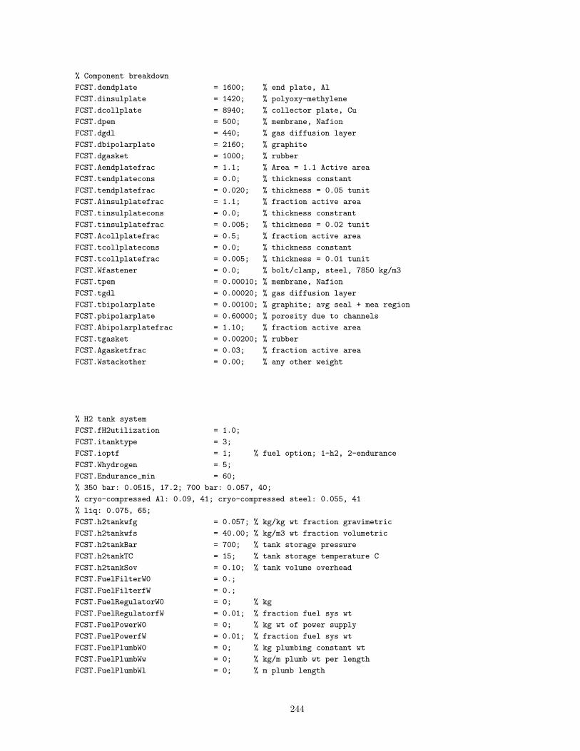
% Component breakdown
FCST.dendplate = 1600; % end plate, Al
FCST.dinsulplate = 1420; % polyoxy-methylene
FCST.dcollplate = 8940; % collector plate, Cu
FCST.dpem = 500; % membrane, Nafion
FCST.dgdl = 440; % gas diffusion layer
FCST.dbipolarplate = 2160; % graphite
FCST.dgasket = 1000; % rubber
FCST.Aendplatefrac = 1.1; % Area = 1.1 Active area
FCST.tendplatecons = 0.0; % thickness constant
FCST.tendplatefrac = 0.020; % thickness = 0.05 tunit
FCST.Ainsulplatefrac = 1.1; % fraction active area
FCST.tinsulplatecons = 0.0; % thickness constrant
FCST.tinsulplatefrac = 0.005; % thickness = 0.02 tunit
FCST.Acollplatefrac = 0.5; % fraction active area
FCST.tcollplatecons = 0.0; % thickness constant
FCST.tcollplatefrac = 0.005; % thickness = 0.01 tunit
FCST.Wfastener = 0.0; % bolt/clamp, steel, 7850 kg/m3
FCST.tpem = 0.00010; % membrane, Nafion
FCST.tgdl = 0.00020; % gas diffusion layer
FCST.tbipolarplate = 0.00100; % graphite; avg seal + mea region
FCST.pbipolarplate = 0.60000; % porosity due to channels
FCST.Abipolarplatefrac = 1.10; % fraction active area
FCST.tgasket = 0.00200; % rubber
FCST.Agasketfrac = 0.03; % fraction active area
FCST.Wstackother = 0.00; % any other weight
% H2 tank system
FCST.fH2utilization = 1.0;
FCST.itanktype = 3;
FCST.ioptf = 1; % fuel option; 1-h2, 2-endurance
FCST.Whydrogen = 5;
FCST.Endurance_min = 60;
% 350 bar: 0.0515, 17.2; 700 bar: 0.057, 40;
% cryo-compressed Al: 0.09, 41; cryo-compressed steel: 0.055, 41
% liq: 0.075, 65;
FCST.h2tankwfg = 0.057; % kg/kg wt fraction gravimetric
FCST.h2tankwfs = 40.00; % kg/m3 wt fraction volumetric
FCST.h2tankBar = 700; % tank storage pressure
FCST.h2tankTC = 15; % tank storage temperature C
FCST.h2tankSov = 0.10; % tank volume overhead
FCST.FuelFilterW0 = 0.;
FCST.FuelFilterfW = 0.;
FCST.FuelRegulatorW0 = 0; % kg
FCST.FuelRegulatorfW = 0.01; % fraction fuel sys wt
FCST.FuelPowerW0 = 0; % kg wt of power supply
FCST.FuelPowerfW = 0.01; % fraction fuel sys wt
FCST.FuelPlumbW0 = 0; % kg plumbing constant wt
FCST.FuelPlumbWw = 0; % kg/m plumb wt per length
FCST.FuelPlumbWl = 0; % m plumb length
244

FCST.Pfuel0 = 0; % prescribed power
FCST.Pfuelk = 0; % prop to fuel flow rate
FCST.Pfuele = 0; % expo to fuel flow rate
FCST.FGErho = 722.13;% density of gasoline
FCST.FGEMJkg = 44; % heating value of gasoline, MJ/kg
FCST.FGEeta = 0.25; % efficiency of FGE fuel
% Air system variables
FCST.fAirFlowRate = 2.5;
FCST.DPstack = 30000; % pres drop in stack, Pa
% Blower
FCST.iBlower = 0;
FCST.BlowEta = 0.75;
FCST.BlowW0 = 0;
FCST.BlowWtf = 1.0;
FCST.BlowWk = 1/1000;
FCST.BlowWfe = 0;
FCST.BlowWpe = 1;
FCST.BlowS0 = 0;
FCST.BlowStf = 1.0;
FCST.BlowSk = 1/3e6;
FCST.BlowSfe = 0;
FCST.BlowSpe = 1;
% Compressor
FCST.iCompressor = 1;
FCST.CompEta = 0.75;
FCST.CompW0 = 0.;
FCST.CompWtf = 1.0;
FCST.CompWk = 7e-4; % 122 kg/kg/s or 7e-4 kg/W
FCST.CompWfe = 0;
FCST.CompWpe = 1;
FCST.CompS0 = 0.;
FCST.CompStf = 1.0;
FCST.CompSk = 4.14e-7; % 0.0722 m3/kg/s or 4.14e-7 m3/W
FCST.CompSfe = 0;
FCST.CompSpe = 1;
% Turbo-expander (axial-flow turbine)
FCST.iTurbine = 1;
FCST.TurbEta = 0.75;
FCST.TurbW0 = 0.;
FCST.TurbWtf = 1.0;
FCST.TurbWk = 0;
FCST.TurbWfe = 0;
FCST.TurbWpe = 0;
FCST.TurbS0 = 0.;
FCST.TurbStf = 1.0;
FCST.TurbSk = 0;
FCST.TurbSfe = 0;
FCST.TurbSpe = 0;
245
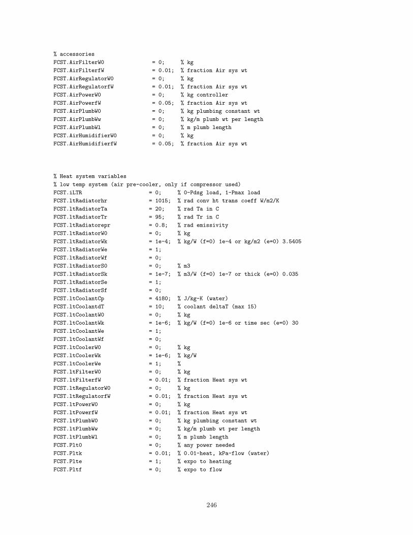
% accessories
FCST.AirFilterW0 = 0; % kg
FCST.AirFilterfW = 0.01; % fraction Air sys wt
FCST.AirRegulatorW0 = 0; % kg
FCST.AirRegulatorfW = 0.01; % fraction Air sys wt
FCST.AirPowerW0 = 0; % kg controller
FCST.AirPowerfW = 0.05; % fraction Air sys wt
FCST.AirPlumbW0 = 0; % kg plumbing constant wt
FCST.AirPlumbWw = 0; % kg/m plumb wt per length
FCST.AirPlumbWl = 0; % m plumb length
FCST.AirHumidifierW0 = 0; % kg
FCST.AirHumidifierfW = 0.05; % fraction Air sys wt
% Heat system variables
% low temp system (air pre-cooler, only if compressor used)
FCST.iLTR = 0; % 0-Pdsg load, 1-Pmax load
FCST.ltRadiatorhr = 1015; % rad conv ht trans coeff W/m2/K
FCST.ltRadiatorTa = 20; % rad Ta in C
FCST.ltRadiatorTr = 95; % rad Tr in C
FCST.ltRadiatorepr = 0.8; % rad emissivity
FCST.ltRadiatorW0 = 0; % kg
FCST.ltRadiatorWk = 1e-4; % kg/W (f=0) 1e-4 or kg/m2 (e=0) 3.5405
FCST.ltRadiatorWe = 1;
FCST.ltRadiatorWf = 0;
FCST.ltRadiatorS0 = 0; % m3
FCST.ltRadiatorSk = 1e-7; % m3/W (f=0) 1e-7 or thick (e=0) 0.035
FCST.ltRadiatorSe = 1;
FCST.ltRadiatorSf = 0;
FCST.ltCoolantCp = 4180; % J/kg-K (water)
FCST.ltCoolantdT = 10; % coolant deltaT (max 15)
FCST.ltCoolantW0 = 0; % kg
FCST.ltCoolantWk = 1e-6; % kg/W (f=0) 1e-6 or time sec (e=0) 30
FCST.ltCoolantWe = 1;
FCST.ltCoolantWf = 0;
FCST.ltCoolerW0 = 0; % kg
FCST.ltCoolerWk = 1e-6; % kg/W
FCST.ltCoolerWe = 1; %
FCST.ltFilterW0 = 0; % kg
FCST.ltFilterfW = 0.01; % fraction Heat sys wt
FCST.ltRegulatorW0 = 0; % kg
FCST.ltRegulatorfW = 0.01; % fraction Heat sys wt
FCST.ltPowerW0 = 0; % kg
FCST.ltPowerfW = 0.01; % fraction Heat sys wt
FCST.ltPlumbW0 = 0; % kg plumbing constant wt
FCST.ltPlumbWw = 0; % kg/m plumb wt per length
FCST.ltPlumbWl = 0; % m plumb length
FCST.Plt0 = 0; % any power needed
FCST.Pltk = 0.01; % 0.01-heat, kPa-flow (water)
FCST.Plte = 1; % expo to heating
FCST.Pltf = 0; % expo to flow
246

% Heat system variables
% high temp system (stack cooling)
FCST.iHV = 0; % 0-LHV, 1-HHV
FCST.iHTR = 0; % 0-Pdsg load, 1-Pmax load
FCST.htStackfd = 0; % stack frac stack heat dissipated
FCST.htStackhs = 3; % stack conv ht trans coeff W/m2/K
FCST.htStackTa = 40; % stack Ta in C
FCST.htStackeps = 0.8; % stack emissivity
FCST.htStackfs = 0.6; % stack frac surface/active area
FCST.htRadiatorhr = 1015; % rad conv ht trans coeff W/m2/K
FCST.htRadiatorTa = 20; % rad Ta in C
FCST.htRadiatorTr = 95; % rad Tr in C
FCST.htRadiatorepr = 0.8; % rad emissivity
FCST.htRadiatorW0 = 0; % kg
FCST.htRadiatorWk = 1e-5; % kg/W (f=0) 1e-5 or kg/m2 (e=0) 3.5405
FCST.htRadiatorWe = 1;
FCST.htRadiatorWf = 0;
FCST.htRadiatorS0 = 0; % m3
FCST.htRadiatorSk = 1e-7; % m3/W (f=0) 1e-7 or thick (e=0) 0.035
FCST.htRadiatorSe = 1;
FCST.htRadiatorSf = 0;
FCST.htCoolantCp = 4180; % J/kg-K (water)
FCST.htCoolantrho = 997; % kg/m3 (water)
FCST.htCoolantdT = 10; % coolant Tc in C
FCST.htCoolantW0 = 0; % kg
FCST.htCoolantWk = 1e-6; % kg/W (f=0) 1e-6 or time sec (e=0) 5
FCST.htCoolantWe = 1;
FCST.htCoolantWf = 0;
FCST.htFilterW0 = 0; % kg
FCST.htFilterfW = 0.01; % fraction Heat sys wt
FCST.htRegulatorW0 = 0; % kg
FCST.htRegulatorfW = 0.01; % fraction Heat sys wt
FCST.htPowerW0 = 0; % kg
FCST.htPowerfW = 0.01; % fraction Heat sys wt
FCST.htPlumbW0 = 0; % kg plumbing constant wt
FCST.htPlumbWw = 0; % kg/m plumb wt per length
FCST.htPlumbWl = 0; % m plumb length
FCST.Pht0 = 0; % any power needed
FCST.Phtk = 0.01; % 0.01-heat, kPa-flow (water)
FCST.Phte = 1; % expo to heat
FCST.Phtf = 0; % expo to coolant flow
% Water system variables
FCST.rhowater = 997; % kg/m3
FCST.waterstoragefrac = 0.2; % fraction of produce stored
FCST.waterstoragehour = 0.5; % accumulated over this time
FCST.watertankSov = 0; % Stank = (1+Sov).Swater
FCST.watertankWov = 0; % Wtank = (1+Wov).Wwater
FCST.waterFilterW0 = 0; % kg
FCST.waterFilterfW = 0; % fraction Heat sys wt
FCST.waterRegulatorW0 = 0; % kg
247
FCST.waterRegulatorfW = 0; % fraction water sys wt
FCST.waterPowerW0 = 0; % kg
FCST.waterPowerfW = 0; % fraction water sys wt
FCST.waterPlumbW0 = 0; % kg plumbing constant wt
FCST.waterPlumbWw = 0; % kg/m plumb wt per length
FCST.waterPlumbWl = 0; % m plumb length
FCST.Pwater0 = 0; % any power needed
FCST.Pwaterk = 1e6; % prop to liq water flow
FCST.Pwatere = 1; % expo to liq water flow
% electrical system variables
FCST.elecControlW0 = 0; % kg
FCST.elecControlWk = 0.01; % prop to stack current
FCST.elecControlWe = 1.0; % expo to stack current
FCST.elecRegulatorW0 = 0; % kg
FCST.elecRegulatorfW = 0; % fraction elec sys wt
FCST.elecPowerW0 = 0; % kg
FCST.elecPowerfW = 0.01; % fraction elec sys wt
FCST.elecPlumbW0 = 0; % kg plumbing constant wt
FCST.elecPlumbWwk = 0.01; % prop to stack current
FCST.elecPlumbWwe = 1.0; % expo to stack current
FCST.elecPlumbWl = 0; % m plumb length
FCST.Pelec0 = 0; % any power needed
FCST.Peleck = 0.02; % prop to stack power
FCST.Pelece = 1.0; % expo to stack power
% additional gross overhead fractions
FCST.fovpower = 0.0;
FCST.fovweight = 0.0;
FCST.fovvolume = 0.0;
% output options
FCST.iplotVIP = 1;
FCST.iprntSCR = 1;
% =====================================================
% O U T P U T S - Design
% =====================================================
% overall weight, power, energy, and specific quantities
% stack efficiencies
FCST.etadsgHHV = 0.;
FCST.etadsgLHV = 0.;
FCST.etamaxHHV = 0.;
FCST.etamaxLHV = 0.;
% net system efficiencies
248

FCST.EtadsgHHV = 0.;
FCST.EtadsgLHV = 0.;
FCST.EtamaxHHV = 0.;
FCST.EtamaxLHV = 0.;
% Fuel gallon equivalents
FCST.FGEHHV = 0.; % chemical
FCST.FGELHV = 0.; % chemical
FCST.FGEHHVtrue = 0.; % engine (chemical x efficiency)
FCST.FGELHVtrue = 0.; % engine (chemical x efficiency)
FCST.Wtotal = 0.;
FCST.Stotal = 0.;
FCST.Wstacksys = 0.;
FCST.Sstacksys = 0.;
FCST.DFstacksys = 0.;
FCST.SFCPdsg_kgkWh = 0.;
FCST.SFCPmax_kgkWh = 0.;
FCST.SFCPdsg_kgkWhe = 0.;
FCST.SFCPmax_kgkWhe = 0.;
FCST.POWERdsg_kWe = 0.;
FCST.POWERmax_kW = 0.;
FCST.POWERmax_kWe = 0.;
FCST.ENERGY_Pdsg_kWh = 0.;
FCST.ENERGY_Pdsg_kWhe = 0.;
FCST.ENERGY_Pmax_kWh = 0.;
FCST.ENERGY_Pmax_kWhe = 0.;
FCST.SPower_Pdsg_Stack_kWkg = 0.;
FCST.SPower_Pdsg_Stack_kWekg = 0.;
FCST.SPower_Pmax_Stack_kWkg = 0.;
FCST.SPower_Pmax_Stack_kWekg = 0.;
FCST.SPower_Pdsg_Stacksys_kWkg = 0.;
FCST.SPower_Pdsg_Stacksys_kWekg= 0.;
FCST.SPower_Pmax_Stacksys_kWkg = 0.;
FCST.SPower_Pmax_Stacksys_kWekg= 0.;
FCST.SPower_Pdsg_kWkg = 0.;
FCST.SPower_Pdsg_kWekg = 0.;
FCST.SPower_Pmax_kWkg = 0.;
FCST.SPower_Pmax_kWekg = 0.;
FCST.EDensity_Pdsg_kWhL = 0.;
FCST.EDensity_Pdsg_kWheL = 0.;
FCST.EDensity_Pmax_kWhL = 0.;
FCST.EDensity_Pmax_kWheL = 0.;
FCST.SEnergy_Pdsg_kWhkg = 0.;
FCST.SEnergy_Pdsg_kWhekg = 0.;
FCST.SEnergy_Pmax_kWhkg = 0.;
FCST.SEnergy_Pmax_kWhekg = 0.;
% Design factor of system
249

FCST.DFsystem = 0.; % cell pc / (P/W) in kW/kg
FCST.DFsysteme = 0.; % cell pc / (P/W) in kWe/kg
% stack variables
% performance
FCST.ivdata = 0.;
FCST.Eh = 0.;
FCST.Er = 0.;
FCST.Aactive_cm2 = 0.;
FCST.Ncell = 0.;
FCST.Istackdsg = 0.;
FCST.Vstackdsg = 0.;
FCST.Istackmax = 0.;
FCST.Vstackmax = 0.;
FCST.IstackPmax = 0.;
FCST.VstackPmax = 0.;
FCST.SP = 0.;
FCST.vcdsg = 0.;
FCST.icdsg = 0.;
FCST.pcdsg = 0.;
FCST.etadsg = 0.;
FCST.etavdsgHHV = 0.;
FCST.etavdsgLHV = 0.;
% size
FCST.Sstack = 0.;
FCST.Lstack = 0.;
FCST.Astack = 0.;
FCST.DFstack = 0.;
Wstack.total = 0.;
Wstack.endplate = 0.;
Wstack.insulplate = 0.;
Wstack.collplate = 0.;
Wstack.unit = 0.;
Wstack.cell = 0.;
Wstack.mea = 0.;
Wstack.bipolarplate = 0.;
Wstack.pem = 0.;
Wstack.gdl = 0.;
Wstack.gasket = 0.;
Wstack.other = 0.;
FCST.Wstack = Wstack;
FCST.Wstackk0 = 0.;
FCST.Wstackk1 = 0.;
% Air system variables
FCST.Sblower = 0.;
FCST.Scomp = 0.;
FCST.Sturb = 0.;
Wair.total = 0.;
Wair.blower = 0.;
Wair.comp = 0.;
250

Wair.turb = 0.;
Wair.precooler = 0.;
Wair.humidifier = 0.;
Wair.filter = 0.;
Wair.plumbing = 0.;
Wair.power = 0.;
Wair.regulator = 0.;
FCST.Wair = Wair;
FCST.Pair_kW = 0.;
FCST.Pairmax_kW = 0.;
FCST.Pblower_kW = 0.;
FCST.Pblowermax_kW = 0.;
FCST.Pcomp_kW = 0.;
FCST.Pcompmax_kW = 0.;
FCST.Pturb_kW = 0.;
FCST.Pturbmax_kW = 0.;
FCST.MassAirrate_kgs = 0.;
FCST.MassAirrate_max_kgs = 0.;
FCST.MassAirrate_Ls = 0.;
FCST.MassAirrate_max_Ls = 0.;
FCST.MassAirrate_out_kgs = 0.;
FCST.MassAirrate_out_max_kgs = 0.;
FCST.Humidity_ratio = 0.;
FCST.MassWaterrate_kgs = 0.;
FCST.MassVaporrate_kgs = 0.;
FCST.MassLiquidrate_kgs = 0.;
% Fuel system variables
FCST.Sh2tank = 0.;
Wfuel.total = 0.;
Wfuel.H2 = 0.;
Wfuel.tank = 0.;
Wfuel.filter = 0.;
Wfuel.plumbing = 0.;
Wfuel.power = 0.;
Wfuel.regulator = 0.;
FCST.Wfuel = Wfuel;
FCST.Pfuel_kW = 0.;
FCST.Pfuelmax_kW = 0.;
FCST.MassH2rate_kgs = 0.;
FCST.MassH2rate_Pmax_kgs = 0.;
FCST.SFCPdsg_kgkWh = 0.;
FCST.SFCPmax_kgkWh = 0.;
% low temp cooling system variables (air pre-cooler)
Wlt.total = 0.;
Wlt.filter = 0.;
Wlt.plumbing = 0.;
Wlt.regulator = 0.;
Wlt.coolant = 0.;
251
Wlt.radiator = 0.;
Wlt.power = 0.;
FCST.Wlt = Wlt;
FCST.Plt_kW = 0.;
FCST.Pltmax_kW = 0.;
FCST.Sltradiator = 0.;
FCST.Altradiator = 0.;
FCST.HEATINGlt_kW = 0.;
FCST.HEATINGlt_max_kW = 0.;
FCST.Cflowmaxlt = 0.;
FCST.Cflowdsglt = 0.;
FCST.Cflowlt = 0.;
% high temp cooling system variables (stack cooler)
Wht.total = 0.;
Wht.filter = 0.;
Wht.plumbing = 0.;
Wht.regulator = 0.;
Wht.coolant = 0.;
Wht.radiator = 0.;
Wht.power = 0.;
FCST.Wht = Wht;
FCST.Pht_kW = 0.;
FCST.Phtmax_kW = 0.;
FCST.Shtradiator = 0.;
FCST.Ahtradiator = 0.;
FCST.HEATINGstack_kW = 0.;
FCST.HEATINGairin_kW = 0.;
FCST.HEATINGairout_kW = 0.;
FCST.HEATINGstack_max_kW = 0.;
FCST.HEATINGairin_max_kW = 0.;
FCST.HEATINGairout_max_kW = 0.;
FCST.HEATINGdiscon_kW = 0.;
FCST.HEATINGdisrad_kW = 0.;
FCST.HEATINGhtc_max_kW = 0.;
FCST.HEATINGhtc_kW = 0.;
FCST.Cflowmaxht = 0.;
FCST.Cflowdsght = 0.;
FCST.Cflowht = 0.;
% Water system
FCST.Swatertank = 0.;
Wwater.total = 0.;
Wwater.tank = 0.;
Wwater.plumbing = 0.;
Wwater.power = 0.;
Wwater.regulator = 0.;
FCST.Wwater = Wwater;
FCST.Pwater_kW = 0.;
FCST.Pwatermax_kW = 0.;
252

FCST.MassTankrate_kgs = 0.;
% Electrical system
Welec.total = 0.;
Welec.controller = 0.;
Welec.power = 0.;
Welec.plumbing = 0.;
FCST.Welec = Welec;
Welec.Pelec_kW = 0.;
Welec.Pelecmax_kW = 0.;
% Other
FCST.Wother = 0.;
FCST.Pother_kW = 0.;
FCST.Sother = 0.;
% =====================================================
% I N P U T S - Operations
% =====================================================
FCOP.Istack = 0;
FCOP.iatm = 0;
FCOP.altitude = 0000*0.3048;
FCOP.temperatureC = 20;
FCOP.BlowEta = 0.75;
FCOP.CompEta = 0.75;
FCOP.TurbEta = 0.75;
FCOP.vcorr = 0; % vc correction
FCOP.vrate1000ft = -0.005; % percent drop / 1000 ft
FCOP.vdropaboveft = 1000; % above 1000-ft
FCOP.arh = FCST.arh;
FCOP.crh = FCST.arh;
% =====================================================
% O U T P U T S - Operations
% =====================================================
FCOP.ivdata = 0;
FCOP.pressure = 0;
FCOP.Vstack = 0;
FCOP.SFC_kgkWh = 0;
FCOP.POWER_kW = 0;
FCOP.Pair_kW = 0;
FCOP.Pfuel_kW = 0;
FCOP.Plt_kW = 0;
FCOP.Pht_kW = 0;
FCOP.Pwater_kW = 0;
253

FCOP.Pelec_kW = 0;
FCOP.Pother_kW = 0;
FCOP.POWER_kWe = 0;
FCOP.Pbop_kW = 0;
FCOP.Pblower_kW = 0;
FCOP.Pcomp_kW = 0;
FCOP.Pturb_kW = 0;
FCOP.etac = 0;
FCOP.etas = 0;
FCOP.Vstack = 0;
FCOP.MassH2rate_kgs = 0;
FCOP.MassAirrate_kgs = 0;
FCOP.MassAirrate_Ls = 0;
FCOP.MassO2rate_kgs = 0;
FCOP.MassAirrate_out_kgs = 0;
FCOP.MassWaterrate_kgs = 0;
FCOP.MassLiquidrate_kgs = 0;
FCOP.MassTankrate_kgs = 0;
FCOP.MassVaporrate_out_kgs = 0;
FCOP.Humidity = 0;
FCOP.HEATINGairin_kW = 0;
FCOP.HEATINGstack_kW = 0;
FCOP.SFCvsPe = 0; % kg/kWe-hr vs kWe
FCOP.H2flowvsPe = 0; % kg/hr vs kg/hr
FCOP.Pevs1000ft = 0; % [kW, h in 1000-ft]
FCOP.SFCvs1000ft = 0; % [kg/kWhe in 1000-ft]
FCOP.H2invs1000ft = 0; % [kg/s, h in 1000-ft]
254

% run Modern 80kW liqcool
% SI units unless otherwise appended
% =====================================================
% I N P U T S - Design
% =====================================================
% design options for power
FCST.ioptp = 3; % option, design power, kW
FCST.POWERdsg_kW = 80; % design stack power, kW
FCST.etac = 0.37; % cell efficiency
FCST.vc = 0.70; % cell voltage, V
FCST.Voltage = 250;
% atmospheric conditions affecting design
FCST.iatm = 0; % environment option
FCST.OneAtm = 101325; % Standard atm, Pa
FCST.temperatureC = 15; % temp of environ, C
FCST.altitudeDesign = 0000*0.3048; % altitude, m
FCST.pressure = 0.0*101325; % pressure, Pa
% cell i-v variables
FCST.TstackC = 80; % stack temp, C
FCST.Pstack = 2.5*101325; % stack pres, Pa
FCST.xO2 = 0.2095; % mole fraction of O2 in air
FCST.ioptiv = 3; % 1-data, 2-make, 3-PMAT
FCST.ivdatainp = [
0 1.1782 0
0.0200 0.8580 0.0172
0.0400 0.8529 0.0341
0.0600 0.8481 0.0509
0.0800 0.8434 0.0675
0.1000 0.8390 0.0839
0.1200 0.8347 0.1002
0.1400 0.8305 0.1163
0.1600 0.8264 0.1322
0.1800 0.8225 0.1481
0.2000 0.8187 0.1637
0.2200 0.8150 0.1793
0.2400 0.8114 0.1947
0.2600 0.8078 0.2100
0.2800 0.8044 0.2252
0.3000 0.8010 0.2403
0.3200 0.7977 0.2553
0.3400 0.7945 0.2701
0.3600 0.7913 0.2849
0.3800 0.7881 0.2995
0.4000 0.7850 0.3140
0.4200 0.7820 0.3284
255

0.4400 0.7790 0.3428
0.4600 0.7761 0.3570
0.4800 0.7732 0.3711
0.5000 0.7703 0.3852
0.5200 0.7675 0.3991
0.5400 0.7647 0.4129
0.5600 0.7619 0.4267
0.5800 0.7592 0.4403
0.6000 0.7565 0.4539
0.6200 0.7538 0.4673
0.6400 0.7511 0.4807
0.6600 0.7485 0.4940
0.6800 0.7459 0.5072
0.7000 0.7433 0.5203
0.7200 0.7407 0.5333
0.7400 0.7381 0.5462
0.7600 0.7356 0.5591
0.7800 0.7331 0.5718
0.8000 0.7306 0.5845
0.8200 0.7281 0.5970
0.8400 0.7256 0.6095
0.8600 0.7231 0.6219
0.8800 0.7207 0.6342
0.9000 0.7182 0.6464
0.9200 0.7158 0.6585
0.9400 0.7134 0.6706
0.9600 0.7109 0.6825
0.9800 0.7085 0.6943
1.0000 0.7061 0.7061
1.0200 0.7037 0.7178
1.0400 0.7013 0.7293
1.0600 0.6989 0.7408
1.0800 0.6965 0.7522
1.1000 0.6941 0.7635
1.1200 0.6917 0.7747
1.1400 0.6893 0.7858
1.1600 0.6869 0.7968
1.1800 0.6845 0.8077
1.2000 0.6821 0.8185
1.2200 0.6797 0.8292
1.2400 0.6773 0.8399
1.2600 0.6749 0.8504
1.2800 0.6725 0.8607
1.3000 0.6700 0.8710
1.3200 0.6676 0.8812
1.3400 0.6651 0.8913
1.3600 0.6627 0.9012
1.3800 0.6602 0.9111
1.4000 0.6577 0.9208
1.4200 0.6552 0.9304
1.4400 0.6527 0.9399
1.4600 0.6501 0.9492
1.4800 0.6476 0.9584
256

1.5000 0.6450 0.9675
1.5200 0.6424 0.9764
1.5400 0.6397 0.9852
1.5600 0.6371 0.9938
1.5800 0.6344 1.0023
1.6000 0.6316 1.0106
1.6200 0.6288 1.0187
1.6400 0.6260 1.0267
1.6600 0.6232 1.0344
1.6800 0.6202 1.0420
1.7000 0.6173 1.0493
1.7200 0.6142 1.0565
1.7400 0.6111 1.0633
1.7600 0.6079 1.0700
1.7800 0.6047 1.0763
1.8000 0.6013 1.0823
1.8200 0.5978 1.0880
1.8400 0.5942 1.0934
1.8600 0.5905 1.0983
1.8800 0.5866 1.1028
1.9000 0.5825 1.1067
1.9200 0.5782 1.1101
1.9400 0.5736 1.1128
1.9600 0.5687 1.1147
1.9800 0.5635 1.1157
2.0000 0.5577 1.1154
2.0200 0.5514 1.1137
2.0400 0.5441 1.1101
2.0600 0.5358 1.1037
2.0800 0.5256 1.0933
2.1000 0.5125 1.0763
2.1200 0.4933 1.0458
2.1400 0.4535 0.9705
];
FCST.ipmaxinp = 100;
FCST.Er = 1.1782;
FCST.j0C = 0.0001;
FCST.alphaC = 0.22;
FCST.j0A = 0.1;
FCST.alphaA = 0.5;
FCST.ASR = 0.04;
FCST.jL = 2.45;
FCST.jleak = 0.30;
FCST.C = 0.35;
FCST.PMAT = [
1 1.25 1.5 2.0 2.5
0.0001 0.0001 0.0001 0.0001 0.0001
0.1800 0.1900 0.2000 0.2100 0.2200
0.1000 0.1000 0.1000 0.1000 0.1000
0.5000 0.5000 0.5000 0.5000 0.5000
0.0400 0.0400 0.0400 0.0400 0.0400
1.7500 1.8500 1.9500 2.2500 2.4500
0.1500 0.1500 0.2000 0.2500 0.3000
257

0.0300 0.0350 0.0350 0.0350 0.0350
];
FCST.crh = 100;
FCST.arh = 100;
FCST.deltai = 0.02;
% temp corr
FCST.ASR0 = 0.12; % ref value
FCST.ASR0t = 80; % ref temp
FCST.ASRtk2 = 0.0006;
FCST.ASRtk1 = 0.002;
FCST.jL0 = 0.73; % ref value
FCST.jL0t = 80; % ref temp
FCST.jLtk2 = -0.0015;
FCST.jLtk1 = -0.003;
% humidity corrections in ASR and jL
FCST.ASR0arh = 100; % ref anode rh
FCST.ASR0crh = 100; % ref cathode rh
FCST.ASRrhk1a = -0.005;
FCST.ASRrhk2a = 0.;
FCST.ASRrhk1a1c = 0.;
FCST.ASRrhk1a2c = 2.0e-6;
FCST.ASRrhk2a2c = 0.;
FCST.ASRrhk2a1c = 0.;
FCST.ASRrhk2c = 7.0e-5;
FCST.ASRrhk1c = 0.0021;
FCST.jL0arh = 100;
FCST.jL0crh = 100;
FCST.jLrhk1a = 0.;
FCST.jLrhk2a = 0.;
FCST.jLrhk1a1c = 0.;
FCST.jLrhk1a2c = 0.;
FCST.jLrhk2a2c = 0.;
FCST.jLrhk2a1c = 0.;
FCST.jLrhk2c = -0.0001;
FCST.jLrhk1c = -0.0076;
% other corrections
FCST.icorr = 0; % ic corr (0/1)
FCST.TFi = 1.0; % changes ic to ic.Tfi
FCST.vcorr = 0; % vc corr for alt (0/1)
FCST.deltav = -0.01; % cell to stack correction
FCST.vrate1000ft = -0.0056; % percent drop / 1000 ft
FCST.vdropaboveft = 1000; % above 1000-ft
% stack weight variables
FCST.TFwstack = 1.0; % Tech factor stack weight
FCST.dWwstack = 0.0; % correction stack weight
FCST.TFsstack = 1.0; % Tech factor stack volume
FCST.dSsstack = 0.0; % correction stack volume
FCST.ioptsw = 1; % 0: simple, 1: detailed
FCST.tcell = 0.001381; % cell thickness, m
FCST.dcell = 2584; % cell density, kg/m3
FCST.porosity = 1.0;
258

% Component breakdown
FCST.dendplate = 1600; % end plate, Al
FCST.dinsulplate = 1420; % polyoxy-methylene
FCST.dcollplate = 8940; % collector plate, Cu
FCST.dpem = 500; % membrane, Nafion
FCST.dgdl = 440; % gas diffusion layer
FCST.dbipolarplate = 2160; % graphite
FCST.dgasket = 1000; % rubber
FCST.Aendplatefrac = 1.1; % Area = 1.1 Active area
FCST.tendplatecons = 0.0; % thickness constant
FCST.tendplatefrac = 0.020; % thickness = 0.05 tunit
FCST.Ainsulplatefrac = 1.1; % fraction active area
FCST.tinsulplatecons = 0.0; % thickness constrant
FCST.tinsulplatefrac = 0.005; % thickness = 0.02 tunit
FCST.Acollplatefrac = 0.5; % fraction active area
FCST.tcollplatecons = 0.0; % thickness constant
FCST.tcollplatefrac = 0.005; % thickness = 0.01 tunit
FCST.Wfastener = 0.0; % bolt/clamp, steel, 7850 kg/m3
FCST.tpem = 0.00010; % membrane, Nafion
FCST.tgdl = 0.00020; % gas diffusion layer
FCST.tbipolarplate = 0.00100; % graphite; avg seal + mea region
FCST.pbipolarplate = 0.60000; % porosity due to channels
FCST.Abipolarplatefrac = 1.10; % fraction active area
FCST.tgasket = 0.00200; % rubber
FCST.Agasketfrac = 0.03; % fraction active area
FCST.Wstackother = 0.00; % any other weight
% H2 tank system
FCST.fH2utilization = 1.0;
FCST.itanktype = 3;
FCST.ioptf = 1; % fuel option; 1-h2, 2-endurance
FCST.Whydrogen = 5;
FCST.Endurance_min = 60;
% 350 bar: 0.0515, 17.2; 700 bar: 0.057, 40;
% cryo-compressed Al: 0.09, 41; cryo-compressed steel: 0.055, 41
% liq: 0.075, 65;
FCST.h2tankwfg = 0.057; % kg/kg wt fraction gravimetric
FCST.h2tankwfs = 40.00; % kg/m3 wt fraction volumetric
FCST.h2tankBar = 700; % tank storage pressure
FCST.h2tankTC = 15; % tank storage temperature C
FCST.h2tankSov = 0.10; % tank volume overhead
FCST.FuelFilterW0 = 0.;
FCST.FuelFilterfW = 0.;
FCST.FuelRegulatorW0 = 0; % kg
FCST.FuelRegulatorfW = 0.01; % fraction fuel sys wt
FCST.FuelPowerW0 = 0; % kg wt of power supply
FCST.FuelPowerfW = 0.01; % fraction fuel sys wt
FCST.FuelPlumbW0 = 0; % kg plumbing constant wt
FCST.FuelPlumbWw = 0; % kg/m plumb wt per length
FCST.FuelPlumbWl = 0; % m plumb length
259

FCST.Pfuel0 = 0; % prescribed power
FCST.Pfuelk = 0; % prop to fuel flow rate
FCST.Pfuele = 0; % expo to fuel flow rate
FCST.FGErho = 722.13;% density of gasoline
FCST.FGEMJkg = 44; % heating value of gasoline, MJ/kg
FCST.FGEeta = 0.25; % efficiency of FGE fuel
% Air system variables
FCST.fAirFlowRate = 2.5;
FCST.DPstack = 30000; % pres drop in stack, Pa
% Blower
FCST.iBlower = 0;
FCST.BlowEta = 0.75;
FCST.BlowW0 = 0;
FCST.BlowWtf = 1.0;
FCST.BlowWk = 1/1000;
FCST.BlowWfe = 0;
FCST.BlowWpe = 1;
FCST.BlowS0 = 0;
FCST.BlowStf = 1.0;
FCST.BlowSk = 1/3e6;
FCST.BlowSfe = 0;
FCST.BlowSpe = 1;
% Compressor
FCST.iCompressor = 1;
FCST.CompEta = 0.75;
FCST.CompW0 = 0.;
FCST.CompWtf = 1.0;
FCST.CompWk = 7e-4; % 122 kg/kg/s or 7e-4 kg/W
FCST.CompWfe = 0;
FCST.CompWpe = 1;
FCST.CompS0 = 0.;
FCST.CompStf = 1.0;
FCST.CompSk = 4.14e-7; % 0.0722 m3/kg/s or 4.14e-7 m3/W
FCST.CompSfe = 0;
FCST.CompSpe = 1;
% Turbo-expander (axial-flow turbine)
FCST.iTurbine = 1;
FCST.TurbEta = 0.75;
FCST.TurbW0 = 0.;
FCST.TurbWtf = 1.0;
FCST.TurbWk = 0;
FCST.TurbWfe = 0;
FCST.TurbWpe = 0;
FCST.TurbS0 = 0.;
FCST.TurbStf = 1.0;
FCST.TurbSk = 0;
FCST.TurbSfe = 0;
FCST.TurbSpe = 0;
260

% accessories
FCST.AirFilterW0 = 0; % kg
FCST.AirFilterfW = 0.01; % fraction Air sys wt
FCST.AirRegulatorW0 = 0; % kg
FCST.AirRegulatorfW = 0.01; % fraction Air sys wt
FCST.AirPowerW0 = 0; % kg controller
FCST.AirPowerfW = 0.05; % fraction Air sys wt
FCST.AirPlumbW0 = 0; % kg plumbing constant wt
FCST.AirPlumbWw = 0; % kg/m plumb wt per length
FCST.AirPlumbWl = 0; % m plumb length
FCST.AirHumidifierW0 = 0; % kg
FCST.AirHumidifierfW = 0.05; % fraction Air sys wt
% Heat system variables
% low temp system (air pre-cooler, only if compressor used)
FCST.iLTR = 1; % 0-Pdsg load, 1-Pmax load
FCST.ltRadiatorhr = 1015; % rad conv ht trans coeff W/m2/K
FCST.ltRadiatorTa = 20; % rad Ta in C
FCST.ltRadiatorTr = 95; % rad Tr in C
FCST.ltRadiatorepr = 0.8; % rad emissivity
FCST.ltRadiatorW0 = 0; % kg
FCST.ltRadiatorWk = 3.5405;% kg/W (f=0) 1e-4 or kg/m2 (e=0) 3.5405
FCST.ltRadiatorWe = 0;
FCST.ltRadiatorWf = 1;
FCST.ltRadiatorS0 = 0; % m3
FCST.ltRadiatorSk = 0.035; % m3/W (f=0) 1e-7 or thick (e=0) 0.035
FCST.ltRadiatorSe = 0;
FCST.ltRadiatorSf = 1;
FCST.ltCoolantCp = 4180; % J/kg-K (water)
FCST.ltCoolantdT = 10; % coolant deltaT (max 15)
FCST.ltCoolantW0 = 0; % kg
FCST.ltCoolantWk = 20; % kg/W (f=0) 1e-6 or time sec (e=0) 5
FCST.ltCoolantWe = 0;
FCST.ltCoolantWf = 1;
FCST.ltCoolerW0 = 0; % kg
FCST.ltCoolerWk = 1e-6; % kg/W
FCST.ltCoolerWe = 1; %
FCST.ltFilterW0 = 0; % kg
FCST.ltFilterfW = 0.01; % fraction Heat sys wt
FCST.ltRegulatorW0 = 0; % kg
FCST.ltRegulatorfW = 0.01; % fraction Heat sys wt
FCST.ltPowerW0 = 0; % kg
FCST.ltPowerfW = 0.01; % fraction Heat sys wt
FCST.ltPlumbW0 = 0; % kg plumbing constant wt
FCST.ltPlumbWw = 0; % kg/m plumb wt per length
FCST.ltPlumbWl = 0; % m plumb length
FCST.Plt0 = 0; % any power needed
FCST.Pltk = 300; % 0.01-heat, kPa-flow (water)
FCST.Plte = 0; % expo to heating
FCST.Pltf = 1; % expo to flow
261

% Heat system variables
% high temp system (stack cooling)
FCST.iHV = 0; % 0-LHV, 1-HHV
FCST.iHTR = 0; % 0-Pdsg load, 1-Pmax load
FCST.htStackfd = 0; % stack frac stack heat dissipated
FCST.htStackhs = 3; % stack conv ht trans coeff W/m2/K
FCST.htStackTa = 40; % stack Ta in C
FCST.htStackeps = 0.8; % stack emissivity
FCST.htStackfs = 0.6; % stack frac surface/active area
FCST.htRadiatorhr = 1015; % rad conv ht trans coeff W/m2/K
FCST.htRadiatorTa = 40; % rad Ta in C
FCST.htRadiatorTr = 95; % rad Tr in C
FCST.htRadiatorepr = 0.8; % rad emissivity
FCST.htRadiatorW0 = 0; % kg
FCST.htRadiatorWk = 3.5405;% kg/W (f=0) 1e-5 or kg/m2 (e=0) 3.5405
FCST.htRadiatorWe = 0;
FCST.htRadiatorWf = 1;
FCST.htRadiatorS0 = 0; % m3
FCST.htRadiatorSk = 0.035; % m3/W (f=0) 1e-7 or thick (e=0) 0.035
FCST.htRadiatorSe = 0;
FCST.htRadiatorSf = 1;
FCST.htCoolantCp = 4180; % J/kg-K (water)
FCST.htCoolantrho = 997; % kg/m3 (water)
FCST.htCoolantdT = 10; % coolant Tc in C
FCST.htCoolantW0 = 0; % kg
FCST.htCoolantWk =20; % kg/W (f=0) 1e-6 or time sec (e=0) 5
FCST.htCoolantWe = 0;
FCST.htCoolantWf = 1;
FCST.htFilterW0 = 0; % kg
FCST.htFilterfW = 0.01; % fraction Heat sys wt
FCST.htRegulatorW0 = 0; % kg
FCST.htRegulatorfW = 0.01; % fraction Heat sys wt
FCST.htPowerW0 = 0; % kg
FCST.htPowerfW = 0.01; % fraction Heat sys wt
FCST.htPlumbW0 = 0; % kg plumbing constant wt
FCST.htPlumbWw = 0; % kg/m plumb wt per length
FCST.htPlumbWl = 0; % m plumb length
FCST.Pht0 = 0; % any power needed
FCST.Phtk = 300; % 0.01-heat, kPa-flow (water)
FCST.Phte = 0; % expo to heat
FCST.Phtf = 1; % expo to coolant flow
% Water system variables
FCST.rhowater = 997; % kg/m3
FCST.waterstoragefrac = 0.2; % fraction of produce stored
FCST.waterstoragehour = 0.5; % accumulated over this time
FCST.watertankSov = 0; % Stank = (1+Sov).Swater
FCST.watertankWov = 0; % Wtank = (1+Wov).Wwater
FCST.waterFilterW0 = 0; % kg
FCST.waterFilterfW = 0; % fraction Heat sys wt
FCST.waterRegulatorW0 = 0; % kg
262

FCST.waterRegulatorfW = 0; % fraction water sys wt
FCST.waterPowerW0 = 0; % kg
FCST.waterPowerfW = 0; % fraction water sys wt
FCST.waterPlumbW0 = 0; % kg plumbing constant wt
FCST.waterPlumbWw = 0; % kg/m plumb wt per length
FCST.waterPlumbWl = 0; % m plumb length
FCST.Pwater0 = 0; % any power needed
FCST.Pwaterk = 1e6; % prop to liq water flow
FCST.Pwatere = 1; % expo to liq water flow
% electrical system variables
FCST.elecControlW0 = 0; % kg
FCST.elecControlWk = 0.01; % prop to stack current
FCST.elecControlWe = 1.0; % expo to stack current
FCST.elecRegulatorW0 = 0; % kg
FCST.elecRegulatorfW = 0; % fraction elec sys wt
FCST.elecPowerW0 = 0; % kg
FCST.elecPowerfW = 0.01; % fraction elec sys wt
FCST.elecPlumbW0 = 0; % kg plumbing constant wt
FCST.elecPlumbWwk = 0.01; % prop to stack current
FCST.elecPlumbWwe = 1.0; % expo to stack current
FCST.elecPlumbWl = 0; % m plumb length
FCST.Pelec0 = 0; % any power needed
FCST.Peleck = 0.02; % prop to stack power
FCST.Pelece = 1.0; % expo to stack power
% additional gross overhead fractions
FCST.fovpower = 0.0;
FCST.fovweight = 0.0;
FCST.fovvolume = 0.0;
% output options
FCST.iplotVIP = 1;
FCST.iprntSCR = 1;
% =====================================================
% O U T P U T S - Design
% =====================================================
% overall weight, power, energy, and specific quantities
% stack efficiencies
FCST.etadsgHHV = 0.;
FCST.etadsgLHV = 0.;
FCST.etamaxHHV = 0.;
FCST.etamaxLHV = 0.;
% net system efficiencies
263

FCST.EtadsgHHV = 0.;
FCST.EtadsgLHV = 0.;
FCST.EtamaxHHV = 0.;
FCST.EtamaxLHV = 0.;
% Fuel gallon equivalents
FCST.FGEHHV = 0.; % chemical
FCST.FGELHV = 0.; % chemical
FCST.FGEHHVtrue = 0.; % engine (chemical x efficiency)
FCST.FGELHVtrue = 0.; % engine (chemical x efficiency)
FCST.Wtotal = 0.;
FCST.Stotal = 0.;
FCST.Wstacksys = 0.;
FCST.Sstacksys = 0.;
FCST.DFstacksys = 0.;
FCST.SFCPdsg_kgkWh = 0.;
FCST.SFCPmax_kgkWh = 0.;
FCST.SFCPdsg_kgkWhe = 0.;
FCST.SFCPmax_kgkWhe = 0.;
FCST.POWERdsg_kWe = 0.;
FCST.POWERmax_kW = 0.;
FCST.POWERmax_kWe = 0.;
FCST.ENERGY_Pdsg_kWh = 0.;
FCST.ENERGY_Pdsg_kWhe = 0.;
FCST.ENERGY_Pmax_kWh = 0.;
FCST.ENERGY_Pmax_kWhe = 0.;
FCST.SPower_Pdsg_Stack_kWkg = 0.;
FCST.SPower_Pdsg_Stack_kWekg = 0.;
FCST.SPower_Pmax_Stack_kWkg = 0.;
FCST.SPower_Pmax_Stack_kWekg = 0.;
FCST.SPower_Pdsg_Stacksys_kWkg = 0.;
FCST.SPower_Pdsg_Stacksys_kWekg= 0.;
FCST.SPower_Pmax_Stacksys_kWkg = 0.;
FCST.SPower_Pmax_Stacksys_kWekg= 0.;
FCST.SPower_Pdsg_kWkg = 0.;
FCST.SPower_Pdsg_kWekg = 0.;
FCST.SPower_Pmax_kWkg = 0.;
FCST.SPower_Pmax_kWekg = 0.;
FCST.EDensity_Pdsg_kWhL = 0.;
FCST.EDensity_Pdsg_kWheL = 0.;
FCST.EDensity_Pmax_kWhL = 0.;
FCST.EDensity_Pmax_kWheL = 0.;
FCST.SEnergy_Pdsg_kWhkg = 0.;
FCST.SEnergy_Pdsg_kWhekg = 0.;
FCST.SEnergy_Pmax_kWhkg = 0.;
FCST.SEnergy_Pmax_kWhekg = 0.;
264

% stack variables
% performance
FCST.ivdata = 0.;
FCST.Eh = 0.;
FCST.Er = 0.;
FCST.Aactive_cm2 = 0.;
FCST.Ncell = 0.;
FCST.Istackdsg = 0.;
FCST.Vstackdsg = 0.;
FCST.Istackmax = 0.;
FCST.Vstackmax = 0.;
FCST.IstackPmax = 0.;
FCST.VstackPmax = 0.;
FCST.SP = 0.;
FCST.vcdsg = 0.;
FCST.icdsg = 0.;
FCST.pcdsg = 0.;
FCST.etadsg = 0.;
FCST.etavdsgHHV = 0.;
FCST.etavdsgLHV = 0.;
% size
FCST.Sstack = 0.;
FCST.Lstack = 0.;
FCST.Astack = 0.;
FCST.DFstack = 0.;
Wstack.total = 0.;
Wstack.endplate = 0.;
Wstack.insulplate = 0.;
Wstack.collplate = 0.;
Wstack.unit = 0.;
Wstack.cell = 0.;
Wstack.mea = 0.;
Wstack.bipolarplate = 0.;
Wstack.pem = 0.;
Wstack.gdl = 0.;
Wstack.gasket = 0.;
Wstack.other = 0.;
FCST.Wstack = Wstack;
FCST.Wstackk0 = 0.;
FCST.Wstackk1 = 0.;
% Air system variables
FCST.Sblower = 0.;
FCST.Scomp = 0.;
FCST.Sturb = 0.;
Wair.total = 0.;
Wair.blower = 0.;
Wair.comp = 0.;
Wair.turb = 0.;
Wair.precooler = 0.;
265

Wair.humidifier = 0.;
Wair.filter = 0.;
Wair.plumbing = 0.;
Wair.power = 0.;
Wair.regulator = 0.;
FCST.Wair = Wair;
FCST.Pair_kW = 0.;
FCST.Pairmax_kW = 0.;
FCST.Pblower_kW = 0.;
FCST.Pblowermax_kW = 0.;
FCST.Pcomp_kW = 0.;
FCST.Pcompmax_kW = 0.;
FCST.Pturb_kW = 0.;
FCST.Pturbmax_kW = 0.;
FCST.MassAirrate_kgs = 0.;
FCST.MassAirrate_max_kgs = 0.;
FCST.MassAirrate_Ls = 0.;
FCST.MassAirrate_max_Ls = 0.;
FCST.MassAirrate_out_kgs = 0.;
FCST.MassAirrate_out_max_kgs = 0.;
FCST.Humidity_ratio = 0.;
FCST.MassWaterrate_kgs = 0.;
FCST.MassVaporrate_kgs = 0.;
FCST.MassLiquidrate_kgs = 0.;
% Fuel system variables
FCST.Sh2tank = 0.;
Wfuel.total = 0.;
Wfuel.H2 = 0.;
Wfuel.tank = 0.;
Wfuel.filter = 0.;
Wfuel.plumbing = 0.;
Wfuel.power = 0.;
Wfuel.regulator = 0.;
FCST.Wfuel = Wfuel;
FCST.Pfuel_kW = 0.;
FCST.Pfuelmax_kW = 0.;
FCST.MassH2rate_kgs = 0.;
FCST.MassH2rate_Pmax_kgs = 0.;
FCST.SFCPdsg_kgkWh = 0.;
FCST.SFCPmax_kgkWh = 0.;
% low temp cooling system variables (air pre-cooler)
Wlt.total = 0.;
Wlt.filter = 0.;
Wlt.plumbing = 0.;
Wlt.regulator = 0.;
Wlt.coolant = 0.;
Wlt.radiator = 0.;
Wlt.power = 0.;
266

FCST.Wlt = Wlt;
FCST.Plt_kW = 0.;
FCST.Pltmax_kW = 0.;
FCST.Sltradiator = 0.;
FCST.Altradiator = 0.;
FCST.HEATINGlt_kW = 0.;
FCST.HEATINGlt_max_kW = 0.;
FCST.Cflowmaxlt = 0.;
FCST.Cflowdsglt = 0.;
FCST.Cflowlt = 0.;
% high temp cooling system variables (stack cooler)
Wht.total = 0.;
Wht.filter = 0.;
Wht.plumbing = 0.;
Wht.regulator = 0.;
Wht.coolant = 0.;
Wht.radiator = 0.;
Wht.power = 0.;
FCST.Wht = Wht;
FCST.Pht_kW = 0.;
FCST.Phtmax_kW = 0.;
FCST.Shtradiator = 0.;
FCST.Ahtradiator = 0.;
FCST.HEATINGstack_kW = 0.;
FCST.HEATINGairin_kW = 0.;
FCST.HEATINGairout_kW = 0.;
FCST.HEATINGstack_max_kW = 0.;
FCST.HEATINGairin_max_kW = 0.;
FCST.HEATINGairout_max_kW = 0.;
FCST.HEATINGdiscon_kW = 0.;
FCST.HEATINGdisrad_kW = 0.;
FCST.HEATINGhtc_max_kW = 0.;
FCST.HEATINGhtc_kW = 0.;
FCST.Cflowmaxht = 0.;
FCST.Cflowdsght = 0.;
FCST.Cflowht = 0.;
% Water system
FCST.Swatertank = 0.;
Wwater.total = 0.;
Wwater.tank = 0.;
Wwater.plumbing = 0.;
Wwater.power = 0.;
Wwater.regulator = 0.;
FCST.Wwater = Wwater;
FCST.Pwater_kW = 0.;
FCST.Pwatermax_kW = 0.;
FCST.MassTankrate_kgs = 0.;
267

% Electrical system
Welec.total = 0.;
Welec.controller = 0.;
Welec.power = 0.;
Welec.plumbing = 0.;
FCST.Welec = Welec;
Welec.Pelec_kW = 0.;
Welec.Pelecmax_kW = 0.;
% Other
FCST.Wother = 0.;
FCST.Pother_kW = 0.;
FCST.Sother = 0.;
% =====================================================
% I N P U T S - Operations
% =====================================================
FCOP.Istack = 0;
FCOP.iatm = 0;
FCOP.altitude = 0000*0.3048;
FCOP.temperatureC = 0;
FCOP.BlowEta = 0.75;
FCOP.CompEta = 0.75;
FCOP.TurbEta = 0.75;
FCOP.vcorr = 0; % vc correction
FCOP.vrate1000ft = -0.005; % percent drop / 1000 ft
FCOP.vdropaboveft = 1000; % above 1000-ft
FCOP.arh = FCST.arh;
FCOP.crh = FCST.arh;
% =====================================================
% O U T P U T S - Operations
% =====================================================
FCOP.ivdata = 0;
FCOP.pressure = 0;
FCOP.Vstack = 0;
FCOP.SFC_kgkWh = 0;
FCOP.POWER_kW = 0;
FCOP.Pair_kW = 0;
FCOP.Pfuel_kW = 0;
FCOP.Plt_kW = 0;
FCOP.Pht_kW = 0;
FCOP.Pwater_kW = 0;
FCOP.Pelec_kW = 0;
FCOP.Pother_kW = 0;
268

FCOP.POWER_kWe = 0;
FCOP.Pbop_kW = 0;
FCOP.Pblower_kW = 0;
FCOP.Pcomp_kW = 0;
FCOP.Pturb_kW = 0;
FCOP.etac = 0;
FCOP.etas = 0;
FCOP.Vstack = 0;
FCOP.MassH2rate_kgs = 0;
FCOP.MassAirrate_kgs = 0;
FCOP.MassAirrate_Ls = 0;
FCOP.MassO2rate_kgs = 0;
FCOP.MassAirrate_out_kgs = 0;
FCOP.MassWaterrate_kgs = 0;
FCOP.MassLiquidrate_kgs = 0;
FCOP.MassTankrate_kgs = 0;
FCOP.MassVaporrate_out_kgs = 0;
FCOP.Humidity = 0;
FCOP.HEATINGairin_kW = 0;
FCOP.HEATINGstack_kW = 0;
FCOP.SFCvsPe = 0; % kg/kWe-hr vs kWe
FCOP.H2flowvsPe = 0; % kg/hr vs kg/hr
FCOP.Pevs1000ft = 0; % [kW, h in 1000-ft]
FCOP.SFCvs1000ft = 0; % [kg/kWhe in 1000-ft]
FCOP.H2invs1000ft = 0; % [kg/s, h in 1000-ft]
269
Top Related