Download - Passive vs. Active Control of Rhythmic Ball Bouncing: The ...€¦ · Passive vs. Active Control of Rhythmic Ball Bouncing: The Role of Visual Information ... Previous work shows

Passive vs. Active Control of Rhythmic Ball Bouncing:The Role of Visual Information

Isabelle A. SieglerUniv Paris-Sud

Benoıt G. BardyUniversity of Montpellier I

William H. WarrenBrown University

The simple task of bouncing a ball on a racket offers a model system for studying how human actors exploitthe physics and information of the environment to control their behavior. Previous work shows that peopletake advantage of a passively stable solution for ball bouncing but can also use perceptual information toactively stabilize bouncing. In this article, we investigate (a) active and passive contributions to the control ofbouncing, (b) the visual information in the ball’s trajectory, and (c) how it modulates the parameters of racketoscillation. We used a virtual ball bouncing apparatus to manipulate the coefficient of restitution � andgravitational acceleration g during steady-state bouncing (Experiment 1) and sudden transitions (Experiment2) to dissociate informational variables. The results support a form of mixed control, based on the half-periodof the ball’s trajectory, in which racket oscillation is actively regulated on every cycle in order to keep thesystem in or near the passively stable region. The mixed control mode may be a general strategy for integratingpassive stability with active stabilization in perception–action systems.

Keywords: perception and action, visual control, rhythmic movement, dynamical systems

Adaptive behavior, by definition, requires the spatiotemporalcoordination of one’s actions with the surrounding environment.Accounting for the organization of adaptive behavior thus dependson understanding the dynamics of the interaction between agentand environment (Warren, 2006). A critical issue is the degree towhich human actors exploit environmental constraints, includingphysical properties and informational variables, in order to achievestable patterns of behavior in a given task. To the extent that theydo so, responsibility for the organization in behavior cannot simplybe attributed to internal neural structure, but must be distributedacross an embodied agent and its environment (Gibson, 1979).

The task of bouncing a ball on a racket offers a deceptivelysimple model system with which to investigate these behavioraldynamics. Rhythmically hitting a ball to a constant height impli-cates the entire cycle of perception and action: when the racketapplies a force to the ball at impact, this alters the state ofthe environment and generates multisensory information about theball’s trajectory, which can reciprocally be used to regulate theracket cycle. The central question is precisely how the actor

exploits the physical and informational constraints of the ball–racket system to stabilize rhythmic bouncing.

Schaal, Atkeson, and Sternad (1996) originally showed that ifthe ball is hit at a particular point in a racket’s harmonic cycle,bouncing is passively stable, that is, will continue to a constantheight indefinitely despite small perturbations, without active per-ceptual control. The evidence indicates that participants indeedprefer the passively stable regime (Sternad, Duarte, Katsumata, &Schaal, 2001), and thus appear to exploit this physical stabilityproperty. However, recent results also show that participants ac-tively stabilize bouncing under some conditions (de Rugy, Wei,Muller, & Sternad, 2003; Morice, Siegler, Bardy, & Warren,2007), implying that they also take advantage of perceptual infor-mation to control the racket oscillation. In the present study we usea virtual bouncing apparatus to investigate three issues: first, thecontributions of active and passive control to the stabilization ofbouncing; second, the visual information that is used for thiscontrol; and third, the parameters of racket oscillation that aremodulated by such information.

Dynamics of Ball Bouncing

The dynamics of bouncing a ball on a racket in one (vertical)dimension was analyzed by Schaal et al. (1996) and Dijkstra,Katsumata, de Rugy, and Sternad (2004). Assuming that racketmotion is harmonic (sinusoidal), the bouncing ball map predictsthe state variables of racket phase �r at impact and ball launchvelocity vb after impact, for given parameter values of the gravi-tational constant g, coefficient of restitution �, racket period Tr,and racket amplitude Ar. The coefficient of restitution representsthe elasticity of the ball-racket system (i.e. the “bounciness” of the

Isabelle A. Siegler, Univ Paris-Sud; Benoıt G. Bardy, University ofMontpellier I; and William H. Warren, Brown University.

This research was supported by the National Science Foundation GrantBCS-0450218 and by the ENACTIVE European Commission network ofexcellence IST #002114. The authors would like to thank Bruno Manteland Antoine Morice for their assistance with the research, and DagmarSternad for helpful discussions.

Correspondence regarding this article should be addressed to IsabelleSiegler, Univ Paris-Sud, Laboratoire Controle Moteur et Perception,UPRES EA 4042, Orsay, F- 91405 Cedex. E-mail: [email protected]

Journal of Experimental Psychology: © 2010 American Psychological AssociationHuman Perception and Performance2010, Vol. 36, No. 3, 729–750

0096-1523/10/$12.00 DOI: 10.1037/a0016462

729

ball with a constant racket). Analysis of the bouncing ball mapdemonstrated the existence of a passive stability regime: If impactoccurs during the last quarter of the racket cycle, when the racket’supward motion has a positive velocity but is decelerating, thenfollowing small perturbations of the ball or racket the system willrelax back to a stable period-1 attractor, with constant values of vb

�r, and bounce height. The bouncing ball system is thus self-stabilizing, such that small errors will die away without activeerror correction.

Specifically, the ball-racket system is passively stable if racketacceleration at impact (ar) remains in the negative range

�2g�1 � �2�

�1 � ��2 � ar � 0. (1)

For example, with � � 0.5 and g � 9.8 m/s2, racket accelerationmust be between �10.9 and 0 m/s2 for passive stability, andanalysis revealed a narrower region of maximal stability between–5 and –2 m/s2. Intuitively, self-stabilization occurs because anupward perturbation of the ball will delay impact with the decel-erating racket, so the racket will have a lower impact velocity andhit the ball to a lower height, yielding an earlier impact in the nextcycle. Over multiple cycles, this compensates for the upwardperturbation; and vice versa for a downward perturbation. Thus,exploiting passive stability obviates the need for active errorcorrection of small perturbations.

Passive or Active Stabilization?

However, the existence of a passively stable regime does notrule out a contribution of active perceptual control. Perceptualinformation may be used to identify the passive regime duringlearning, to initialize the system in the passive region at the onsetof bouncing, or to maintain ongoing bouncing. The first aim of thepresent study was to determine the mode of control used tomaintain bouncing, specifically how it combines active and pas-sive stabilization.

At one extreme is (a) the pure passive control hypothesis, whichargues that bouncing is maintained through passive stabilizationalone in an open-loop fashion, without relying on perceptualinformation. At the other extreme is (b) the pure active controlhypothesis, that perceptual information is used to actively stabilizebouncing on every cycle in a closed-loop fashion, without regardto passive stability. One example is the “mirror algorithm” inwhich racket velocity symmetrically mirrors ball velocity, yieldingbouncing outside the passively stable range, with positive impactaccelerations (Buhler, Koditschek, & Kindlmann, 1994). An inter-mediate hypothesis is what we will call (c) hybrid control, inwhich small perturbations are passively stabilized while largeperturbations outside the passive range are actively stabilized. Thisimplies a threshold at the stability boundary where perceptualcontrol is initiated, based on the magnitude of the perturbation.Finally, (d) the mixed control hypothesis proposes that activestabilization exploits the passive physics of the task. On this view,bouncing is perceptually controlled on each cycle in order to keepthe system in or near the passively stable region, thereby reducingthe magnitude of racket adjustment and increasing stability.

Initial reports confirmed that experienced participants tend tobounce in the passively stable region, with negative impact accel-

erations clustered in the maximally stable range (Schaal et al.,1996; Sternad et al., 2001). In addition, the variability of impactacceleration and ball amplitude were lowest in the maximallystable range, as expected. With practice, impact accelerationsbecame progressively negative over trials and converged to themaximally stable region (Sternad et al., 2001). This evidenceindicates that actors exploit passive stability, consistent with thepassive control hypothesis.

However, subsequent reports found that bouncing could also besustained in the unstable region, with positive impact accelera-tions, implicating a form of active control (Siegler, Mantel,Warren, & Bardy, 2003; Morice et al., 2007). To probe thispossibility, de Rugy et al. (2003) perturbed the coefficient ofrestitution � at single impacts during ongoing bouncing (equiva-lent to perturbing the launch velocity), destabilizing the system ona majority of trials. They observed that participants rapidly com-pensated for large perturbations by adjusting the period of racketoscillation, so that impact acceleration and phase returned to thepassively stable range within two to three cycles. These results aresuggestive of hybrid control, in which perturbations beyond thepassively stable range are actively corrected.

While this article was in preparation, Wei, Dijkstra, and Sternad(2007) reported a study that manipulated both large and small pertur-bations in �. They again found relaxation times of only two to threecycles, much more rapid than predicted by passive stabilization(Dijsktra et al., 2004). Moreover, they observed that racket adjust-ments were proportional to the magnitude of perturbation within aswell as beyond the stable region, consistent with active control. Butthere were also traces of passive stability, for bouncing generallyreturned to the negative acceleration range, larger perturbations re-quired longer relaxation times, and decreases in � yielded longerrelaxation times than increases in �. They interpreted these results asevidence for a “blend” of active and passive stabilization.

More recently, Wei, Dijkstra, and Sternad (2008) looked for thepresence of active control components when the task was performedat steady state in different stability conditions (by varying � from 0.3to 0.9). Wei et al (2008) interpreted significant differences betweenthe autocovariance functions of the predictions of the passive stabilitymodel and the data as differences in the time needed to compensatefor errors and therefore as the presence of active control components.Yet, significant differences were only exhibited for high values of �(� � 0.6), which lead to very bouncy balls and the most unstableconditions. This main analysis did not show that active control waspresent at lower values of �. Wei et al. (2008) also performedregressions between perceptual variables and action variables. As theyobserved that the slopes were more negative when calculated on theexperimental data than on the model data, for all participants and all� values, Wei et al. (2008) concluded that participants did use activeerror compensation. However, these two analyses appear to be incon-sistent for the more stable conditions, and further studies are neededto gain insight into this important question.

Thus, taken together, the existing pattern of data is most consistentwith the mixed control hypothesis, by which bouncing is activelycontrolled on every cycle to keep the system within or near thepassively stable region. Here we test the hypotheses using a converg-ing approach, by manipulating g as well as � and analyzing thedependency of racket adjustments on the ball’s trajectory.

730 SIEGLER, BARDY, AND WARREN

Information for Active Control

These findings implicate a role for perceptual information in theactive control of bouncing. The second aim of the present study wasthus to determine the optical variables of the ball’s trajectory that areused for active stabilization. A number of variables are potentiallyinformative about the timing of the upcoming impact, and thus couldbe used to regulate the period and phase of racket oscillation. Theyinclude (a) visual information in the ball’s trajectory; (b) hapticinformation about the time and force of the current impact; (c)acoustic information about the time, and possibly the force, of thecurrent impact; and (d) combinations of the above variables.

In the first investigation of informational variables, Sternad et al.(2001) withdrew either visual or haptic information once the partici-pant had achieved stable bouncing on each trial. Surprisingly, withonly haptic (and acoustic) information available, bouncing could bemaintained at the optimal mean negative impact acceleration, al-though its variability increased significantly compared to a full-information control. This demonstrates that haptic (and acoustic)information is sufficient to sustain bouncing in the passively stableregion, but it also implies a stabilizing role for vision. Conversely,bouncing could also be maintained with only visual (and acoustic)information available, although the mean impact acceleration wasclose to zero (marginally stable), and its variability again increased.This result implies that haptic information also plays a stabilizing roleand more accurately specifies the maximally stable region. Finally,Morice et al. (2007) found that bouncing can be maintained outsidethe passively stable region with vision alone, confirming that visualinformation is sufficient for active stabilization.

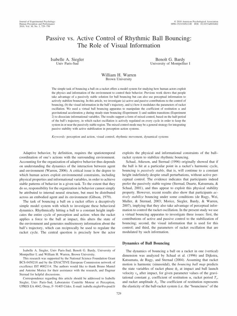
We can formalize the information these variables offer to spec-ify the time-to-impact (refer to Figure 1). Assume that ball massmb, coefficient of restitution �, and gravitational acceleration g areconstant under given conditions, and that contact with the racketoccurs at a constant height (hc). To stabilize bouncing, the agentmust hit the returning ball at a particular phase in the racket cycle

(�r) when racket acceleration is negative. Hence, useful temporalinformation would specify the period of the ball’s flight fromimpact to impact (Tb), or the time from the peak of flight until theball returns to the contact height (tdown).

First, consider haptic information (the derivation appears in Ap-pendix A). The ball’s ith flight period Ti, relative to the previousperiod Ti � 1, is proportional to the force Fi and duration �ti ofcontact,

Ti � �Ti�1 �2Fi�ti

gmb(2)

where F�t � I is the impulse at impact. Thus, for a given ball thechange in the upcoming flight period is specified by haptic infor-mation about the impact impulse. This information could be usedto adjust racket period to match flight period and maintain aconstant impact phase. To determine whether this solution isstable, the haptic system would also have to determine the accel-eration and phase at the moment of impact from proprioceptionabout arm motion. Note, however, that Eq. 2 depends on � and g,and thus the information would have to be rescaled to new con-ditions over multiple bounces. In principle, haptic informationcould thus account for the ability to maintain stable bouncing aftervision is withdrawn (Sternad et al., 2001), although it is insuffi-cient to initialize bouncing with an unknown ball or to rapidlycorrect for ball perturbations during flight.

Second, acoustic variables specify the moment of impact, andsound intensity may provide information about the force of impact.Thus, analogous to Eq. 2, acoustic information could also be usedto determine the change in flight period and maintain stablebouncing, although not to initialize bouncing or rapidly correct forperturbations during flight.

Third, there are a number of optical variables from the ball’strajectory that could be used to determine the time-to-impact andto correct for perturbations during flight. We identified four can-didate hypotheses, most of which depend on g (derivations appearin Appendix B).

(i) Launch velocity. Assuming that g is known, the ball’sflight time (period Tb) is specified by its launch velocity vb. Halfof this value corresponds to the downward flight time from thepeak to the contact height (tdown):

tdown �vb

gor Tb �

2vb

g(3)

(ii) Peak height. Given that g is known, the downward flighttime is determined by its peak height hp. The flight period is twicethis value:

tdown � �2hp

gor Tb � 2�2hp

g(4)

Note that the visually perceived height may also depend on theperceived distance of the ball, or on other aspects of the visualcontext. When astronauts in zero-g conditions were asked to catcha falling ball travelling at a constant velocity, McIntyre, Zago,Berthoz, and Lacquaniti (2001) reported that they were adapted toearth’s gravitational acceleration (g � 9.81 m/s2), and henceresponded too early. This suggests that participants could useheight information to control bouncing if g is implicitly known.

Figure 1. Definition of variables for racket motion (solid line, subscript r)and ball trajectory (broken lines, subscript b). C0 labels the racket cyclecontaining a key event; in Experiment 2, g transitions occur at the ball peakduring C0, and � transitions occur at impact just prior to C0. tup0 and tdown0

refer to upward and downward ball flight (dashed line) during C0. Racketcycles can be subclassified into four quarter-cycles, corresponding tophases of acceleration and deceleration.

731PASSIVE VS. ACTIVE CONTROL OF BALL BOUNCING

(iii) Half-period. The duration of the downward half-periodof the ball’s flight from peak to contact (tdown) is equal to that ofthe upward half-period from contact to peak (tup). The total flightperiod is thus twice this value:

tdown � tup or Tb � 2tup. (5)

It is important that this relationship does not depend on g, aslong it remains constant during the ball’s flight. This gives us ameans of dissociating the half-period hypothesis from the otherinformational variables.

(iv) Tau-gap. During the ball’s descent, the movement of theracket could be guided by the tau of the motion-gap, that is, therate of closure of the spatial gap between the ball and the racketpositions. The tau-gap �c is the first-order time-to-closure of themotion-gap, i.e., the current size of the motion-gap x divided by itscurrent rate of closure x (Lee, 1976; Bootsma & Oudejans, 1993):

�c � x/x. (6)

Unless g is additionally taken into account, this variable over-estimates the actual time-to-closure, but it converges as the ballapproaches the contact height.

In the present experiments, we sought to determine the effectivevisual information in the ball’s trajectory. Three of the ball variablesdescribed above depend upon a known g, whereas half-period infor-mation does not: the duration of the downward half-period of theball’s trajectory is the same as that of the upward half-period regard-less of g. We thus dissociated these variables by changing g to a newconstant value at the peak of the ball’s trajectory, which allowed us totest several hypotheses. First, if participants rely on peak height (hp),launch velocity (vb), or tau-gap (�c), they would have to relearn a newimplicit value of g over a number of bounces, and should thus exhibitpredictable errors in racket timing following a transition in g.McIntyre et al.’s (2001) observation that astronauts failed to adapt tozero-g conditions in 90 trials of ball catching implies that g may notbe quickly relearned. Second, if participants rely on the duration of theupward half-period (tup), they should rapidly adapt racket motion tothe new value of g, possibly within one cycle. Third, because a suddenchange in � at impact does not alter the informativeness of any ofthese variables, it should elicit rapid adaptation regardless of theinformation used. Finally, pure passive control should produce noracket adjustments after g or � transitions, and error should increaseon subsequent bounces. Correlations between ball variables andracket variables thus allow us to make inferences about the effectivevisual information.

The Racket Oscillator

The third aim of this study was to determine the parameters ofracket motion that are modulated during active control, in order tocharacterize the racket oscillator. The bouncing task involvesrhythmic movement of the forearm about the elbow, which can bemodeled as a nonlinear oscillator defined over neuromuscular andbiomechanical components. As a first approximation, racket oscil-lation can be described by three variables: period, amplitude, andphase, various combinations of which can yield a given racketvelocity at impact. To maintain bouncing to a constant targetheight h, the required racket velocity at impact (vr) is strongly

constrained by the environmental parameters �, g, and h, asfollows:

vr �� 1

� � 1�2gh (7)

(Note that impact velocity is not completely determined byenvironmental conditions, because the racket height at impact andthe bouncing error to the target may also vary.) For sustainedaccurate bouncing, we can identify the following constraints on theracket variables. First, the racket period should approximate theball’s flight period, which is strongly dependent on g and h (byEquation 4). Second, the racket phase at impact may theoreticallyvary, but to satisfy passive stability it should be constrained to theupward decelerating quarter-cycle of racket motion. Third, given aperiod and phase, racket amplitude should be adjusted to producethe impact velocity demanded by �, g, and h (Equation 7). Note,however, that the relation among these three racket variables mayvary as long as they generate the required impact velocity.

A dynamical modeling strategy was pioneered by Kay, Kelso,Saltzman, and Schoner (1987) in a study of wrist oscillation. Asthe pacing frequency was increased using a metronome, theyobserved a monotonic decrease in the amplitude of wrist move-ment and a monotonic increase in peak velocity. The minimalmodel that could account for these data was a hybrid limit cycleoscillator with nonlinear damping. The damping component in-cluded a Rayleigh term that depended on position and captured theamplitude effect, and a Van der Pol term that depended on velocityand captured the peak velocity effect. It is important that both theseeffects of frequency were reproduced by changing a single controlparameter, the oscillator’s stiffness coefficient.

Beek, Rikkert, and van Wieringen (1996) sought to generalizethe model to rhythmic forearm movements about the elbow. Aspacing frequency increased, they also observed that amplitudedecreased in all participants, whereas peak velocity increased inonly a minority of participants and decreased in the majority. Toaccount for the latter group, Beek et al. (1996) proposed a revisedRayleigh term that depends on frequency as well as position. A keyquestion for models of bouncing is thus whether racket amplitudeand period are related, as observed by Kay et al. (1987) and Beeket al. (1996), or can be controlled independently.

Such models suggest that rhythmic movements might be per-ceptually controlled by coupling informational variables to oscil-lator control variables (Warren, 2006); the control variables mayeither be state variables (Schoner, 1991) or parameters (Bingham,2004; Kay & Warren, 2001). In the case of bouncing, racket periodmight be controlled by using visual information about the ball’sflight period to modulate a stiffness parameter, racket phase byadditional information about the previous impact phase, and racketamplitude by visual information about the error to the target. Forinstance, de Rugy et al. (2003) modeled racket motion using aneural half-center oscillator and compensated for perturbations byusing the ball’s launch velocity, which specifies it’s flight period(Eq. 3), to reset the oscillator period. This served to maintain thedesired impact phase and restore the period of bouncing over thenext several cycles. However, an empirical control model willdepend on both the form of the oscillator and the informationactually used to regulate it. By investigating the effective visual


information and how it modulates the racket oscillator, we seek toconstrain the relevant class of models.

We studied the modulation of racket parameters by varying theenvironmental conditions � and g and testing the following pre-dictions, under the constraint of bouncing to a constant targetheight. First, with an increase in g one would expect a compen-satory decrease in racket period, possibly accompanied by adjust-ments in amplitude and/or phase to produce the required impactvelocity. Second, with an increase in �, one would expect acompensatory decrease in racket amplitude to produce the requiredvelocity, but no shift in racket period. An observed independence(or dependence) of racket period and amplitude would place con-straints on the relevant class of model oscillators. Finally, corre-lations between ball variables and racket variables should allow usto infer the coupling of visual information to control parameters.

We conducted two experiments to investigate the mode ofcontrol during bouncing, the information used, and how it modu-lated the racket oscillator. In Experiment 1, we examined steady-state bouncing under various environmental conditions with con-stant values of g and �. In Experiment 2, we examined adaptationof racket oscillation to sudden changes in g or �.

General Methods

Participants

Thirteen participants (27.8 5.3 years) were tested in the twoexperiments presented here. They were informed about the exper-imental procedure and signed a consent form. Participants hadpreviously taken part in one or two ball-bouncing experiments, andthus had learned how to produce stable bouncing (Sternad et al.,2001).

Apparatus

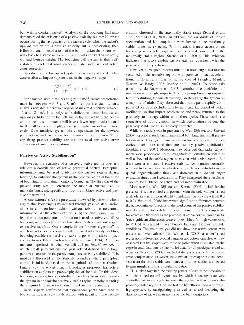
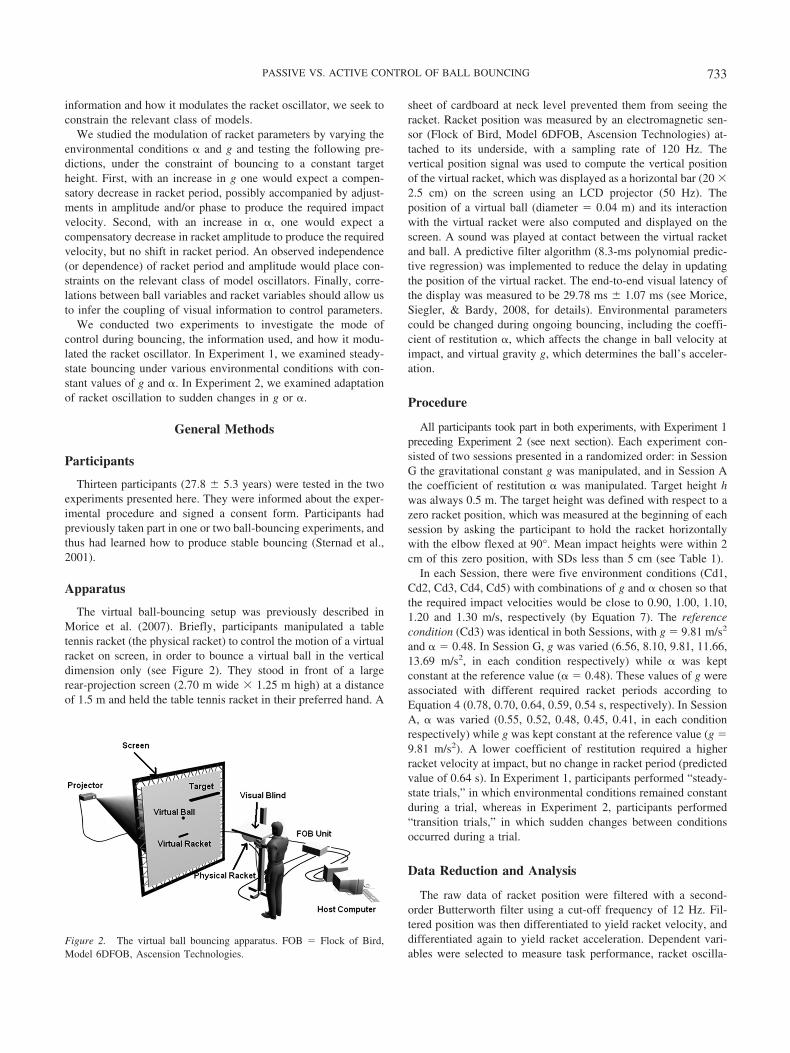
The virtual ball-bouncing setup was previously described inMorice et al. (2007). Briefly, participants manipulated a tabletennis racket (the physical racket) to control the motion of a virtualracket on screen, in order to bounce a virtual ball in the verticaldimension only (see Figure 2). They stood in front of a largerear-projection screen (2.70 m wide 1.25 m high) at a distanceof 1.5 m and held the table tennis racket in their preferred hand. A

sheet of cardboard at neck level prevented them from seeing theracket. Racket position was measured by an electromagnetic sen-sor (Flock of Bird, Model 6DFOB, Ascension Technologies) at-tached to its underside, with a sampling rate of 120 Hz. Thevertical position signal was used to compute the vertical positionof the virtual racket, which was displayed as a horizontal bar (20 2.5 cm) on the screen using an LCD projector (50 Hz). Theposition of a virtual ball (diameter � 0.04 m) and its interactionwith the virtual racket were also computed and displayed on thescreen. A sound was played at contact between the virtual racketand ball. A predictive filter algorithm (8.3-ms polynomial predic-tive regression) was implemented to reduce the delay in updatingthe position of the virtual racket. The end-to-end visual latency ofthe display was measured to be 29.78 ms 1.07 ms (see Morice,Siegler, & Bardy, 2008, for details). Environmental parameterscould be changed during ongoing bouncing, including the coeffi-cient of restitution �, which affects the change in ball velocity atimpact, and virtual gravity g, which determines the ball’s acceler-ation.

Procedure

All participants took part in both experiments, with Experiment 1preceding Experiment 2 (see next section). Each experiment con-sisted of two sessions presented in a randomized order: in SessionG the gravitational constant g was manipulated, and in Session Athe coefficient of restitution � was manipulated. Target height hwas always 0.5 m. The target height was defined with respect to azero racket position, which was measured at the beginning of eachsession by asking the participant to hold the racket horizontallywith the elbow flexed at 90°. Mean impact heights were within 2cm of this zero position, with SDs less than 5 cm (see Table 1).

In each Session, there were five environment conditions (Cd1,Cd2, Cd3, Cd4, Cd5) with combinations of g and � chosen so thatthe required impact velocities would be close to 0.90, 1.00, 1.10,1.20 and 1.30 m/s, respectively (by Equation 7). The referencecondition (Cd3) was identical in both Sessions, with g � 9.81 m/s2

and � � 0.48. In Session G, g was varied (6.56, 8.10, 9.81, 11.66,13.69 m/s2, in each condition respectively) while � was keptconstant at the reference value (� � 0.48). These values of g wereassociated with different required racket periods according toEquation 4 (0.78, 0.70, 0.64, 0.59, 0.54 s, respectively). In SessionA, � was varied (0.55, 0.52, 0.48, 0.45, 0.41, in each conditionrespectively) while g was kept constant at the reference value (g �9.81 m/s2). A lower coefficient of restitution required a higherracket velocity at impact, but no change in racket period (predictedvalue of 0.64 s). In Experiment 1, participants performed “steady-state trials,” in which environmental conditions remained constantduring a trial, whereas in Experiment 2, participants performed“transition trials,” in which sudden changes between conditionsoccurred during a trial.

Data Reduction and Analysis

The raw data of racket position were filtered with a second-order Butterworth filter using a cut-off frequency of 12 Hz. Fil-tered position was then differentiated to yield racket velocity, anddifferentiated again to yield racket acceleration. Dependent vari-ables were selected to measure task performance, racket oscilla-

Figure 2. The virtual ball bouncing apparatus. FOB � Flock of Bird,Model 6DFOB, Ascension Technologies.


tion, and ball/racket impact. Performance was characterized by theerror in bouncing to the target (ε) defined as the difference be-tween the midpoint of the ball at its peak position and target height,and by the racket velocity at impact (vr). Racket oscillation wascharacterized by the cycle period (Tr), defined as the time betweentwo successive peak racket positions, and racket cycle amplitude(Ar), defined as the difference between successive valley and peakracket positions (Sternad et al., 2001; De Rugy, et al., 2003).Ball/racket impact was characterized by the phase in the racketcycle at impact (�r), calculated as the ratio between the time ofimpact in the racket cycle and the cycle period, and the racketacceleration at impact (ar).

A racket cycle (Ci) was defined by two successive maximumracket positions (see Figure 1). For convenience, racket cycleswere numbered from a discrete event such as a transition or animpact, where C0 refers to the cycle that immediately follows thekey event, C�1 refers to the preceding cycle, and C1, C2 . . . , referto the subsequent cycles (Figure 1).

Experiment 1: Steady-State Bouncing

In Experiment 1, we examined how racket oscillation dependson environmental parameters g and � during steady-state bounc-ing. We manipulated g and � between trials but held their valuesconstant within a trial. Our first aim was to determine whetherracket parameters can be independently controlled, to gain insightinto appropriate model oscillators. We expected higher values of gto yield a compensatory decrease in racket period, and perhapscorresponding shifts in racket amplitude and/or impact phase.Conversely, we expected higher values of � to yield a compensa-tory decrease in racket amplitude but no change in racket period.Finally, if participants exploit passive stability, we would expectthe impact acceleration to remain in the passive range.

Our second aim was to begin investigating the coupling ofinformational variables in the ball’s trajectory to parameters of

racket oscillation. Recall that the informativeness of launch veloc-ity and peak height depend on an implicitly known value of g,whereas that of flight period does not; these variables are thusdissociated by varying g. Consequently, correlations between vari-ables of the ball’s trajectory and variables of racket motion com-puted across g conditions may reveal the information used tocontrol bouncing, under the assumption that participants do notrapidly learn a new value of g during one trial.

Method

In Session A and Session G, subjects first performed two prac-tice trials in the reference condition, followed by one test trial ineach of the five environment conditions in a random order. Eachtrial lasted 40 s. For analysis, the first 8 s of data were removedfrom each trial to eliminate transients. The dependent variableswere then measured for each remaining racket cycle, and thesevalues were averaged to yield means for each trial.

Results

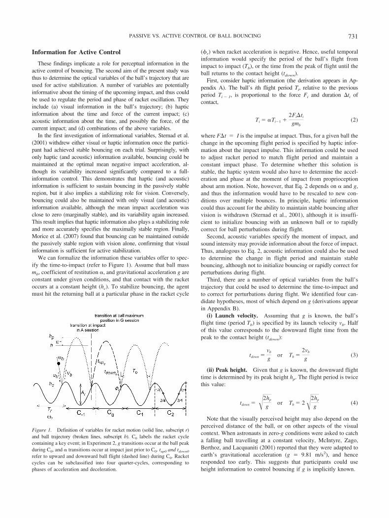
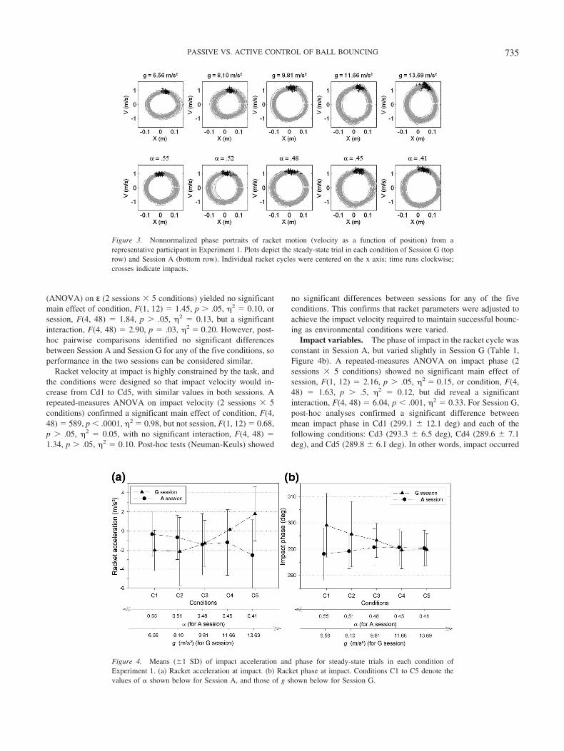
Data from a representative participant are presented in phaseportraits (non-normalized) in Figure 3, which plot racket velocityas a function of racket position. Note that impact (black crosses)tends to occur near or just after the peak (upward) racket velocity,and that the size and shape of the portrait change systematicallywith g and �. A summary of the means and standard deviations ofall dependent variables appears in Table 1.

Task performance: error and racket velocity at impact.Participants could sustain quite accurate bouncing under all con-ditions, with constant errors around �2 cm and standard deviationsabout 0.5 cm. Looking first at the mean bouncing error (ε),participants bounced the ball approximately 2 cm above the target,consistent with aligning the bottom of the 4 cm diameter ball withthe target line. A two-way repeated measures analysis of variance

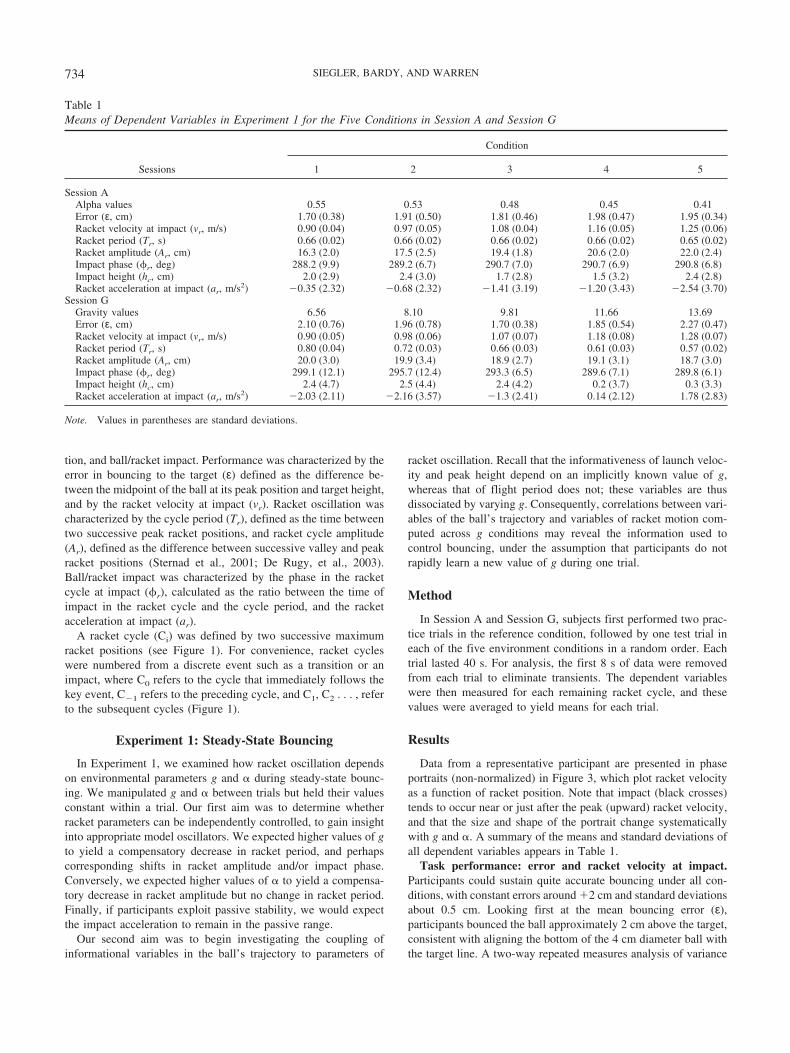
Table 1Means of Dependent Variables in Experiment 1 for the Five Conditions in Session A and Session G

Sessions

Condition

1 2 3 4 5

Session AAlpha values 0.55 0.53 0.48 0.45 0.41Error (ε, cm) 1.70 (0.38) 1.91 (0.50) 1.81 (0.46) 1.98 (0.47) 1.95 (0.34)Racket velocity at impact (vr, m/s) 0.90 (0.04) 0.97 (0.05) 1.08 (0.04) 1.16 (0.05) 1.25 (0.06)Racket period (Tr, s) 0.66 (0.02) 0.66 (0.02) 0.66 (0.02) 0.66 (0.02) 0.65 (0.02)Racket amplitude (Ar, cm) 16.3 (2.0) 17.5 (2.5) 19.4 (1.8) 20.6 (2.0) 22.0 (2.4)Impact phase (�r, deg) 288.2 (9.9) 289.2 (6.7) 290.7 (7.0) 290.7 (6.9) 290.8 (6.8)Impact height (hc, cm) 2.0 (2.9) 2.4 (3.0) 1.7 (2.8) 1.5 (3.2) 2.4 (2.8)Racket acceleration at impact (ar, m/s2) �0.35 (2.32) �0.68 (2.32) �1.41 (3.19) �1.20 (3.43) �2.54 (3.70)

Session GGravity values 6.56 8.10 9.81 11.66 13.69Error (ε, cm) 2.10 (0.76) 1.96 (0.78) 1.70 (0.38) 1.85 (0.54) 2.27 (0.47)Racket velocity at impact (vr, m/s) 0.90 (0.05) 0.98 (0.06) 1.07 (0.07) 1.18 (0.08) 1.28 (0.07)Racket period (Tr, s) 0.80 (0.04) 0.72 (0.03) 0.66 (0.03) 0.61 (0.03) 0.57 (0.02)Racket amplitude (Ar, cm) 20.0 (3.0) 19.9 (3.4) 18.9 (2.7) 19.1 (3.1) 18.7 (3.0)Impact phase (�r, deg) 299.1 (12.1) 295.7 (12.4) 293.3 (6.5) 289.6 (7.1) 289.8 (6.1)Impact height (hc, cm) 2.4 (4.7) 2.5 (4.4) 2.4 (4.2) 0.2 (3.7) 0.3 (3.3)Racket acceleration at impact (ar, m/s2) �2.03 (2.11) �2.16 (3.57) �1.3 (2.41) 0.14 (2.12) 1.78 (2.83)

Note. Values in parentheses are standard deviations.


(ANOVA) on ε (2 sessions 5 conditions) yielded no significantmain effect of condition, F(1, 12) � 1.45, p � .05, 2 � 0.10, orsession, F(4, 48) � 1.84, p � .05, 2 � 0.13, but a significantinteraction, F(4, 48) � 2.90, p � .03, 2 � 0.20. However, post-hoc pairwise comparisons identified no significant differencesbetween Session A and Session G for any of the five conditions, soperformance in the two sessions can be considered similar.

Racket velocity at impact is highly constrained by the task, andthe conditions were designed so that impact velocity would in-crease from Cd1 to Cd5, with similar values in both sessions. Arepeated-measures ANOVA on impact velocity (2 sessions 5conditions) confirmed a significant main effect of condition, F(4,48) � 589, p � .0001, 2 � 0.98, but not session, F(1, 12) � 0.68,p � .05, 2 � 0.05, with no significant interaction, F(4, 48) �1.34, p � .05, 2 � 0.10. Post-hoc tests (Neuman-Keuls) showed

no significant differences between sessions for any of the fiveconditions. This confirms that racket parameters were adjusted toachieve the impact velocity required to maintain successful bounc-ing as environmental conditions were varied.

Impact variables. The phase of impact in the racket cycle wasconstant in Session A, but varied slightly in Session G (Table 1,Figure 4b). A repeated-measures ANOVA on impact phase (2sessions 5 conditions) showed no significant main effect ofsession, F(1, 12) � 2.16, p � .05, 2 � 0.15, or condition, F(4,48) � 1.63, p � .5, 2 � 0.12, but did reveal a significantinteraction, F(4, 48) � 6.04, p � .001, 2 � 0.33. For Session G,post-hoc analyses confirmed a significant difference betweenmean impact phase in Cd1 (299.1 12.1 deg) and each of thefollowing conditions: Cd3 (293.3 6.5 deg), Cd4 (289.6 7.1deg), and Cd5 (289.8 6.1 deg). In other words, impact occurred

Figure 3. Nonnormalized phase portraits of racket motion (velocity as a function of position) from arepresentative participant in Experiment 1. Plots depict the steady-state trial in each condition of Session G (toprow) and Session A (bottom row). Individual racket cycles were centered on the x axis; time runs clockwise;crosses indicate impacts.

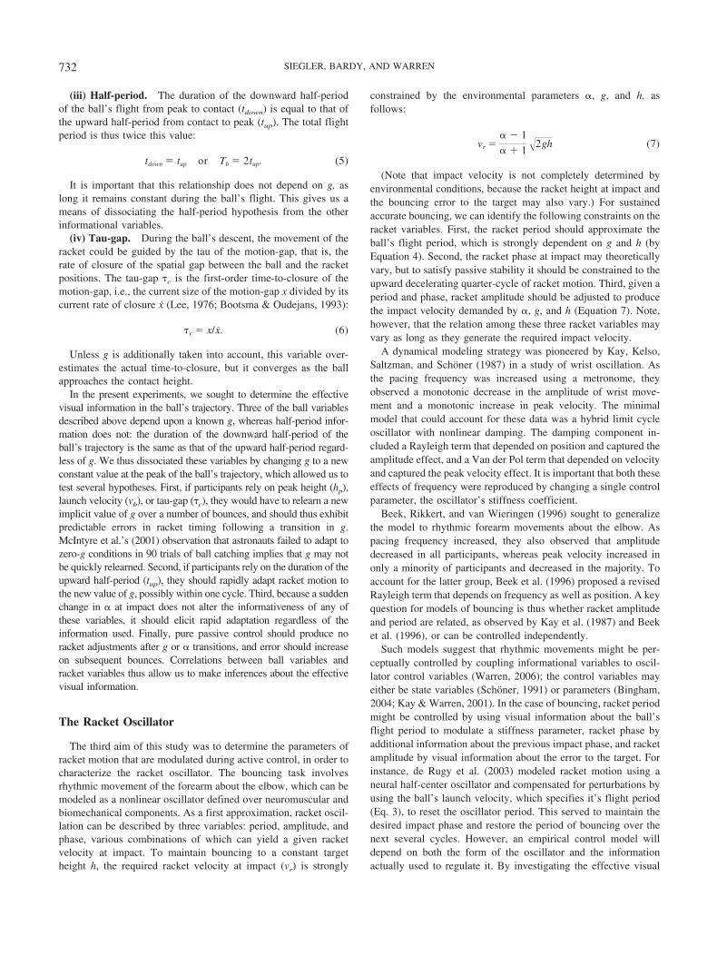
Figure 4. Means (1 SD) of impact acceleration and phase for steady-state trials in each condition ofExperiment 1. (a) Racket acceleration at impact. (b) Racket phase at impact. Conditions C1 to C5 denote thevalues of � shown below for Session A, and those of g shown below for Session G.


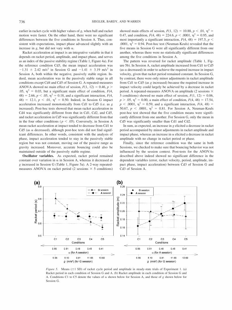
earlier in racket cycle with higher values of g, when ball and racketmotion were faster. On the other hand, there were no significantdifferences between the five conditions in Session A. Thus, con-sistent with expectations, impact phase advanced slightly with anincrease in g, but did not vary with �.

Racket acceleration at impact is an integrative variable in that itdepends on racket period, amplitude, and impact phase, and servesas an index of the passive stability regime (Table 1, Figure 4a). Forthe reference condition Cd3, the mean impact acceleration was�1.31 2.42 m/s2 in Session G and �1.41 3.19 m/s2 inSession A, both within the negative, passively stable region. In-deed, mean acceleration was in the passively stable range in allconditions except Cd4 and Cd5 of Session G. A repeated-measuresANOVA showed no main effect of session, F(1, 12) � 0.46, p �.05, 2 � 0.03, but a significant main effect of condition, F(4,48) � 2.66, p � .05, 2 � 0.18, and a significant interaction, F(4,48) � 12.1, p � .01, 2 � 0.50. Indeed, in Session G impactacceleration increased monotonically from Cd1 to Cd5 (i.e. as gincreased). Post-hoc tests showed that mean racket acceleration inCd4 was significantly different from that in Cd1, Cd2, and Cd5,and racket acceleration in Cd5 was significantly different from thatin the four other conditions ( p � .05). Conversely, in Session Amean racket acceleration at impact tended to decrease from Cd1 toCd5 (as � decreased), although post-hoc tests did not find signif-icant differences. In other words, consistent with the analysis ofphase, impact acceleration tended to stay in the passively stableregion but was not constant, moving out of the passive range asgravity increased. Moreover, accurate bouncing could also bemaintained outside of the passively stable regime.

Oscillator variables. As expected, racket period remainedconstant over variation in � in Session A, whereas it decreased asg increased in Session G (Table 1, Figure 5a). A 2-way repeated-measures ANOVA on racket period (2 sessions 5 conditions)

showed main effects of session, F(1, 12) � 10.88, p � .01, 2 �0.47, and condition, F(4, 48) � 224.6, p � .0001, 2 � 0.95, andmost importantly a significant interaction, F(4, 48) � 197.5, p �.0001, 2 � 0.94. Post-hoc test (Neuman-Keuls) revealed that thefive means in Session G were all significantly different from oneanother, whereas there were no statistically significant differencesamong the five conditions in Session A.

The pattern was reversed for racket amplitude (Table 1, Fig-ure 5b). In Session A, racket amplitude increased from Cd1 to Cd5(as � decreased) in order to achieve the required increase in impactvelocity, given that racket period remained constant. In Session G,by contrast, there were only minor adjustments in racket amplitudefrom Cd1 to Cd5 (as g increased) because the required increase inimpact velocity could largely be achieved by a decrease in racketperiod. A repeated-measures ANOVA on amplitude (2 sessions 5 conditions) showed no main effect of session, F(1, 12) � 0.06,p � .05, 2 � 0.00, a main effect of condition, F(4, 48) � 17.54,p � .0001, 2 � 0.59, and a significant interaction, F(4, 48) �50.67, p � .0001, 2 � 0.81. For Session A, Neuman-Keulspost-hoc test showed that the five condition means were signifi-cantly different from one another. For Session G, only the mean inCd5 was significantly smaller than Cd1 and Cd2.

In sum, as expected, an increase in g elicited a decrease in racketperiod accompanied by minor adjustments in racket amplitude andimpact phase, whereas an increase in � elicited a decrease in racketamplitude with no change in racket period or phase.

Finally, since the reference condition was the same in bothSessions, we checked to make sure that bouncing behavior was notinfluenced by the session context. Post-tests for the ANOVAsdescribed above indeed showed no significant difference in thedependent variables (error, racket velocity, period, amplitude, im-pact phase, impact acceleration) between Cd3 of Session G andCd3 of Session A.

Figure 5. Means (1 SD) of racket cycle period and amplitude in steady-state trials of Experiment 1. (a)Racket period in each condition of Session G and A. (b) Racket amplitude in each condition of Session G andA. Conditions C1 to C5 denote the values of � shown below for Session A, and those of g shown below forSession G.


Covariation of oscillator variables. In order to assess thedependencies among racket oscillator variables, correlations andlinear regressions were performed between racket amplitude (Ar),racket frequency (�r), and peak racket velocity (vmax) on everycycle (we tested frequency rather than period to be comparablewith the literature on rhythmic movement). In Session A, whereracket amplitude decreased with � but g remained constant, therewas no correlation between amplitude and frequency (N � 65, R ��0.05, R2 � 0.003). In contrast, in Session G, where racketfrequency increased with g, we find a significant negative corre-lation between amplitude and frequency (N � 65, R � �0.33,R2 � 0.11, Ar � 0.27 – 0.05 �r, p � .01). However, the correlationcoefficient is quite small, reflecting the constraints on amplitudefor the task of bouncing to a target height. This analysis confirmedthe observation that racket parameters for frequency and amplitudedo not necessarily covary, but can be controlled independently.

Second, if racket motion is approximately harmonic [y ��Ar/ 2�cos�2��rt�], we would expect that peak velocity is propor-tional to amplitude with a coefficient of ��r � 4.77s�1. Indeed, inSession A, peak velocity and amplitude were significantly corre-lated (N � 65, R � 0.84, R2 � 0.7) with a regression slope closeto the predicted value (vmax � 0.31 � 4.44Ar m/s, p � .001).Similarly, in Session G, given that both frequency and impactvelocity increased with g, it is not surprising to obtain a positiverelationship between �r and vmax [N � 65, r � .65, r2 � 0.42,vmax � 0.39 � 0.52 �r, p � .001].

Correlations Between Information Variables and RacketOscillation

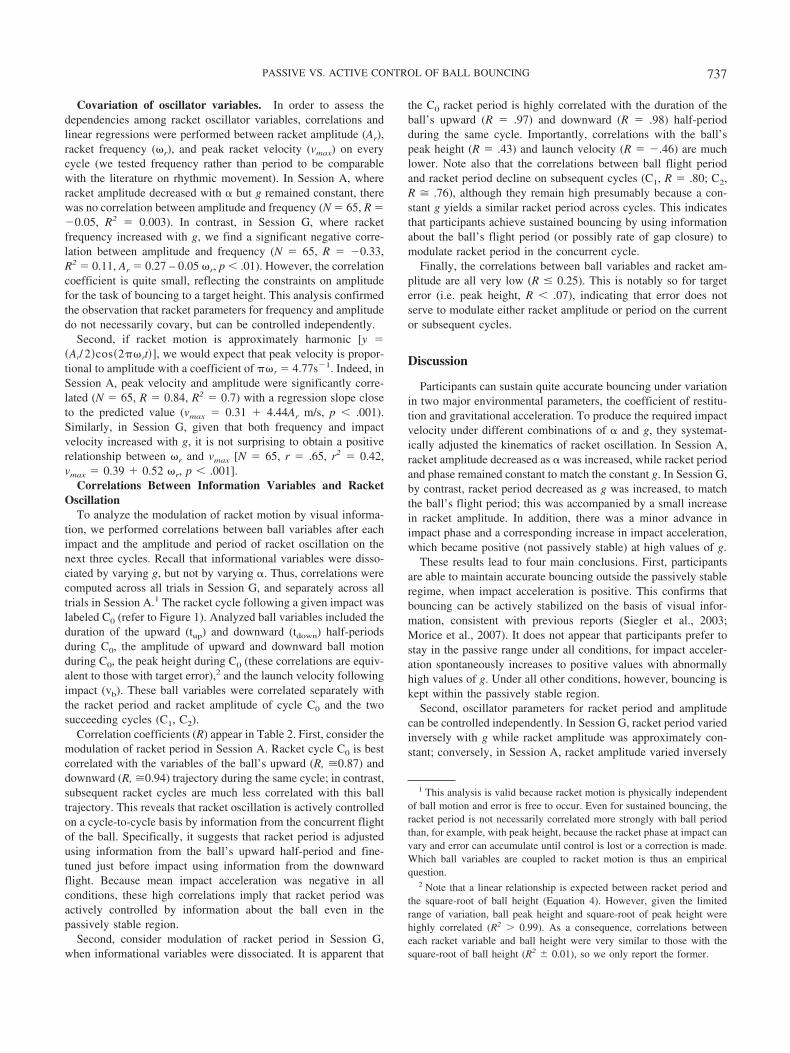
To analyze the modulation of racket motion by visual informa-tion, we performed correlations between ball variables after eachimpact and the amplitude and period of racket oscillation on thenext three cycles. Recall that informational variables were disso-ciated by varying g, but not by varying �. Thus, correlations werecomputed across all trials in Session G, and separately across alltrials in Session A.1 The racket cycle following a given impact waslabeled C0 (refer to Figure 1). Analyzed ball variables included theduration of the upward (tup) and downward (tdown) half-periodsduring C0, the amplitude of upward and downward ball motionduring C0, the peak height during C0 (these correlations are equiv-alent to those with target error),2 and the launch velocity followingimpact (vb). These ball variables were correlated separately withthe racket period and racket amplitude of cycle C0 and the twosucceeding cycles (C1, C2).

Correlation coefficients (R) appear in Table 2. First, consider themodulation of racket period in Session A. Racket cycle C0 is bestcorrelated with the variables of the ball’s upward (R, �0.87) anddownward (R, �0.94) trajectory during the same cycle; in contrast,subsequent racket cycles are much less correlated with this balltrajectory. This reveals that racket oscillation is actively controlledon a cycle-to-cycle basis by information from the concurrent flightof the ball. Specifically, it suggests that racket period is adjustedusing information from the ball’s upward half-period and fine-tuned just before impact using information from the downwardflight. Because mean impact acceleration was negative in allconditions, these high correlations imply that racket period wasactively controlled by information about the ball even in thepassively stable region.

Second, consider modulation of racket period in Session G,when informational variables were dissociated. It is apparent that

the C0 racket period is highly correlated with the duration of theball’s upward (R � .97) and downward (R � .98) half-periodduring the same cycle. Importantly, correlations with the ball’speak height (R � .43) and launch velocity (R � �.46) are muchlower. Note also that the correlations between ball flight periodand racket period decline on subsequent cycles (C1, R � .80; C2,R � .76), although they remain high presumably because a con-stant g yields a similar racket period across cycles. This indicatesthat participants achieve sustained bouncing by using informationabout the ball’s flight period (or possibly rate of gap closure) tomodulate racket period in the concurrent cycle.

Finally, the correlations between ball variables and racket am-plitude are all very low (R � 0.25). This is notably so for targeterror (i.e. peak height, R � .07), indicating that error does notserve to modulate either racket amplitude or period on the currentor subsequent cycles.

Discussion

Participants can sustain quite accurate bouncing under variationin two major environmental parameters, the coefficient of restitu-tion and gravitational acceleration. To produce the required impactvelocity under different combinations of � and g, they systemat-ically adjusted the kinematics of racket oscillation. In Session A,racket amplitude decreased as � was increased, while racket periodand phase remained constant to match the constant g. In Session G,by contrast, racket period decreased as g was increased, to matchthe ball’s flight period; this was accompanied by a small increasein racket amplitude. In addition, there was a minor advance inimpact phase and a corresponding increase in impact acceleration,which became positive (not passively stable) at high values of g.

These results lead to four main conclusions. First, participantsare able to maintain accurate bouncing outside the passively stableregime, when impact acceleration is positive. This confirms thatbouncing can be actively stabilized on the basis of visual infor-mation, consistent with previous reports (Siegler et al., 2003;Morice et al., 2007). It does not appear that participants prefer tostay in the passive range under all conditions, for impact acceler-ation spontaneously increases to positive values with abnormallyhigh values of g. Under all other conditions, however, bouncing iskept within the passively stable region.

Second, oscillator parameters for racket period and amplitudecan be controlled independently. In Session G, racket period variedinversely with g while racket amplitude was approximately con-stant; conversely, in Session A, racket amplitude varied inversely

1 This analysis is valid because racket motion is physically independentof ball motion and error is free to occur. Even for sustained bouncing, theracket period is not necessarily correlated more strongly with ball periodthan, for example, with peak height, because the racket phase at impact canvary and error can accumulate until control is lost or a correction is made.Which ball variables are coupled to racket motion is thus an empiricalquestion.

2 Note that a linear relationship is expected between racket period andthe square-root of ball height (Equation 4). However, given the limitedrange of variation, ball peak height and square-root of peak height werehighly correlated (R2 � 0.99). As a consequence, correlations betweeneach racket variable and ball height were very similar to those with thesquare-root of ball height (R2 0.01), so we only report the former.


with � while racket period remained constant. This was a conse-quence of the task constraints, for it was advantageous for racketperiod to match the flight period of the ball determined by aconstant g, in which case racket amplitude had to vary with � toofor the ball to reach the target. We did observe a small inverserelationship between frequency (�r � 1/Tr) and amplitude inSession G, as amplitude decreased slightly in Cd5, consistent withprevious results for unconstrained rhythmic movement (Kay et al.,1987; Beek et al., 1996). However, there was no such relationshipin Session A. These results imply that a model of unconstrainedmovements in which frequency and amplitude are coupled andcontrolled by a single parameter, such as the stiffness coefficient inthe hybrid Rayleigh-van der Pol (Kay et al., 1987), would notsimply transfer to movements with strong task constraints. At leasttwo control parameters that independently modulate frequency andamplitude are called for.

Third, racket oscillation is actively controlled on a cycle-by-cycle basis. High correlations between ball and racket variablesindicate that information about the ball’s trajectory influencesracket oscillation in the same cycle. It is important to point out thatthese cycle-by-cycle adjustments occurred during steady-statebouncing in the passively stable region. This is consistent with themixed control hypothesis, in which perceptual regulation plays acontinuous role, rather than the hybrid control hypothesis, in whichactive adjustments only occur to correct for perturbations outsidethe stable range.

Finally, we can draw some preliminary conclusions about thevisual information that is used to control racket parameters. Ball-racket correlations indicate that racket period is modulated by thedurations of the upward and downward ball flight in the samecycle, rather than by its peak height or launch velocity. This resultsuggests that the ball’s ascending half-period regulates a parametercontrolling the frequency of racket oscillation. Such an informa-tional coupling would explain how participants successfully

matched racket period to ball period under varying gravitationalconditions. In addition, it is possible that the tau-gap during theball’s descent might be used to fine-tune the racket period, al-though this result could also be due to the necessary correlationbetween the upward and downward half-periods of the ball’sflight. We seek to test this question in Experiment 2. On the otherhand, racket amplitude does not seem to be regulated by any of thestudied ball variables including, somewhat surprisingly, error tothe target on one bounce.

This analysis depends on the fact that informational variableswere dissociated by varying g between trials and assumes thatparticipants do not learn a new value of g during a 40-s trial,consistent with McIntyre et al. (2001). But if they were able to doso, the present pattern of correlations could result from reliance onpeak height or launch velocity corrected by an implicitly knownvalue of g (Equations 3 and 4). Thus, in Experiment 2 we probedthe informational variables by applying sudden changes in g and �within a trial and analyzing immediate adjustments in racketoscillation.

Experiment 2: Adaptation to Sudden Changes

In Experiment 2, we investigated the control of bouncing byrandomly changing an environmental parameter during ongoingbouncing, referred to as transition trials. The purpose of the ex-periment was twofold: to determine the mode of perceptual controland the information it relies on.

First, we sought another test of the hypotheses of passive andactive control by determining whether the racket oscillation isadjusted within one cycle following a sudden change in g or �.Some transitions are destabilizing, in that they take the system intothe unstable region, while others are stabilizing, in that they bring(or leave) the system into the passively stable region. On the pureactive control hypothesis, we would expect rapid adjustments after

Table 2Correlations Between Ball Variables and Racket Variables in Experiment 1, for Three Successive Racket Cycles in Session Aand Session G

Session

All conditions

Racket cycle period Racket cycle amplitude

C0 C1 C2 C0 C1 C2

Session ABall variables

Up half-period (tup0) .86 .32 .20 .05 �.06 �.03 (ns)Down half-period (tdown0) .93 .32 .22 .04 �.06 �.03 (ns)Peak height (hp) .81 .17 .05 �.02 �.13 (ns) �.10Launch velocity (vb) .87 .32 .21 .05 �.06 �.03 (ns)N 2,810

Session GBall variables

Up half-period (tup0) 0.97 0.80 0.75 0.25 0.21 0.23Down half-period (tdown0) 0.98 0.80 0.76 0.25 0.21 0.24Peak height (hp) 0.43 0.06 �0.02 (ns) 0.07 �0.02 (ns) 0.04Launch velocity (vb) �0.46 �0.61 �0.65 0.02 (ns) �0.02 (ns) 0.00 (ns)N 2,781

Note. Unless indicated otherwise (not significant [ns]), all correlations are significant ( p � .05). N � Number of studied cycles; C0 � cycle thatimmediately follows the key event; C1, C2 � subsequent cycles.


all transition types, but they may or may not act to move thesystem into the stable range. On the mixed control hypothesis,adjustments following destabilizing transitions should move thesystem back into the passively stable range, and those followingstabilizing transitions should keep the system in that range. Fi-nally, on the hybrid control hypothesis, we would expect activeadjustments only after destabilizing transitions, not stabilizingtransitions.

Our second purpose was to probe the visual information used toregulate racket adjustments. The results of Experiment 1 suggestthat racket period is modulated by the ball’s flight period in thesame racket cycle, assuming that participants did not learn the newvalue of g within one trial. Here we conduct a more sensitive testby measuring ball-racket correlations in the first few racket cyclesafter a transition, before participants had time to interact with theball and learn the new value of g. If participants take significantlylonger to recover steady-state performance in Session G than inSession A, it would suggest that they use visual information thatdepends on g to control bouncing; if there is no difference betweenSessions, it would suggest that the effective information does notdepend on g.

Moreover, correlations between ball and racket variables imme-diately after a g transition may reveal the information used. Ifparticipants rely on peak height or launch velocity, their correla-tions with racket period should be high in the first cycle after atransition, while the correlations between flight period and racketperiod should be lower, resulting in increased error. Conversely, ifparticipants rely on the duration of the ball’s upward half-period orgap closure during the downward half-period, their correlationswith racket period should be higher than those for peak height andlaunch velocity. In contrast, all correlations should be relativelystrong following an � transition, because it does not dissociate theinformation.

Methods

The five environment conditions (Cd1 to Cd5) in Session A andSession G had the same values of g and � as in Experiment 1, sothe required pre- and posttransition racket velocities were equatedacross sessions. Participants performed 12 transition trials in eachsession, with three transitions per trial. A trial lasted 80 s and wascomposed of four phases with durations of 16 or 24 s, therebyrandomly varying the time between transitions. The first and thirdphases always presented the reference condition (Cd3, g � 9.81,� � .48) whereas the second and fourth phases presented one ofthe other conditions. Thus, in Session G there were two small andtwo large transitions that increased g and two small and two largetransitions that decreased g (see Table 3); correspondingly, inSession A there were four transitions that decreased � and four thatincreased �. Transitions from the reference condition to otherconditions were each presented six times per session, and thereverse transitions were each presented three times per session.

In Session G, the value of g was changed at the ball’s maximumposition in racket cycle C0, thereby dissociating its upward half-period from its downward half-period (refer to Figure 2). InSession A, the value of � was changed at the impact immediatelybefore C0. In the analysis, dependent variables were averagedacross trials to yield a mean for the transition cycle (C0), and forpreceding (C�1) and succeeding (C1, . . .) cycles. The two sessionsoccurred in a random order, and trials were presented in a randomorder within sessions.

Results

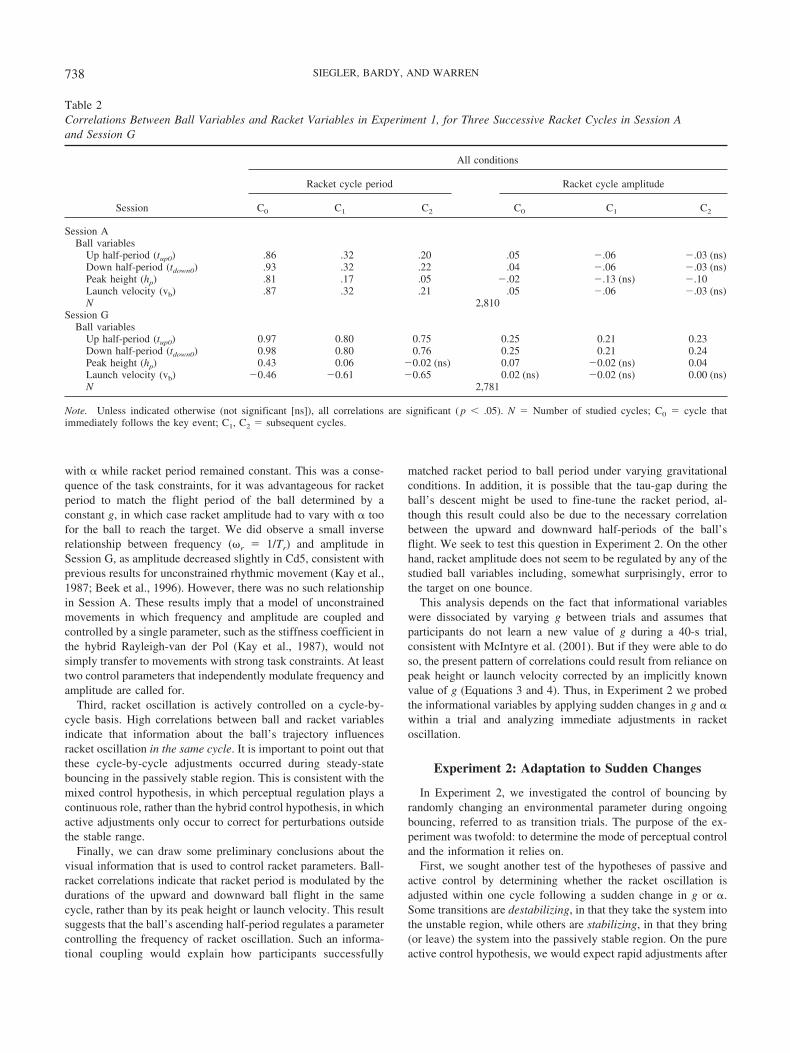
Stabilizing and destabilizing transitions. The mean acceler-ation on the last impact before (Impact �1) and first impact after(Impact 0) the transition is reported in Table 3 (see also Figure 6).

Table 3Characteristics of Transitions in Experiment 2, Session A and Session G

Sessions Transition type N Height F(df) pPlateaubounce

Racket accelerationbefore transition

Racket accelerationafter transition

Session ADecrease � large .553.48 39 F(8, 304) � 8.80 p � .0001� 3 �1.65 (5.16) �1.21 (6.71)Small .523.48 39 F(8, 304) � 6.63 p � .0001� 2 �1.07 (6.03) �0.04 (7.25)Small .483.45b 78 F(8, 616) � 4.82 p � .0001� 4 �1.09 (5.71) �1.59 (6.31)�

Large .483.41 78 F(8, 616) � 18.4 p � .0001� 4 �0.70 (6.04) 0.45 (8.32)Increase � large .413.48b 39 F(8, 304) � 10.0 p � .0001� 2 �1.35 (6.28) �2.66 (5.74)�

Small .453.48b 39 F(8, 304) � 1.68 p � .1 0 �0.89 (7.12) �1.98 (5.11)�

Small .483.52b 78 F(8, 616) � 6.26 p � .0001� 2 �0.55 (6.45) �2.37 (5.80)�

Large .483.55b 78 F(8, 616) � 13.8 p � .0001� 4 �0.10 (5.72) �2.40 (5.43)�

Session GIncrease g large 6.5639.81a 39 F(8, 304) � 15.3 p � .0001� 2 �1.76 (5.46) 4.52 (4.03)�

Small 8.1039.81a 39 F(8, 304) � 5.65 p � .0001� 1 �1.53 (4.38)� 1.77 (4.08)�

Small 9.81311.66a 78 F(8, 616) � 6.71 p � .01� 3 �0.93 (5.52) 2.91 (6.32)�

Large 9.81313.69a 78 F(8, 616) � 41.7 p � .0001� 5 �1.55 (6.51)� 5.66 (5.98)�

Decrease g large 13.6939.81b 39 F(8, 304) � 3.54 p � .001� 1 3.39 (7.82)� �8.88 (6.36)�

Small 11.6639.81b 39 F(8, 304) � 5.08 p � .0001� 1 0.42 (5.98) �3.78 (5.98)�

Small 9.8138.10b 78 F(8, 616) � 2.34 p � .02� 1 0.47 (6.51) �4.86 (5.92)�

Large 9.8136.56b 78 F(8, 616) � 1.71 p � .09 0 �0.15 (6.51) �7.56 (4.43)�

Note. Number of transitions (N). Results of ANOVAs on error (cycles 0 to 8) for each transition type; number of cycles after C0 before plateau of accuratebouncing is reached; and mean racket acceleration at impact during C�1 (before transition) and C0 (after transition).a Take out of stable region. b Bring into stable region.� Significant change in error across cycles.


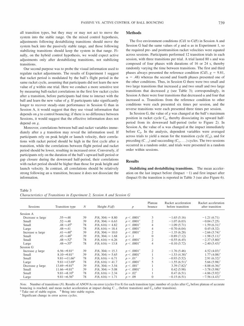
To classify transition types as stabilizing or destabilizing, weperformed one-sample t tests to determine whether the meanimpact acceleration before and after the transition was statisticallydifferent from zero (see Table 3). In Session G, all four increasesin g were destabilizing, taking the system into the significantlypositive range ( p � .05), whereas all four decreases in g werestabilizing, bringing the system into the significantly negativerange ( p � .05). In Session A, none of the transitions weresignificantly destabilizing, whereas all increases in � andone decrease (.483.45) were stabilizing, bringing the systeminto the significantly negative range ( p � .05); the other threetransitions were neutral, not significantly different from zero

before or after the transition. Note that impact acceleration tendedto return toward the negative range following a destabilizingtransition (Figure 6b) and remain in the negative range after astabilizing transition (Figure 6a, c).

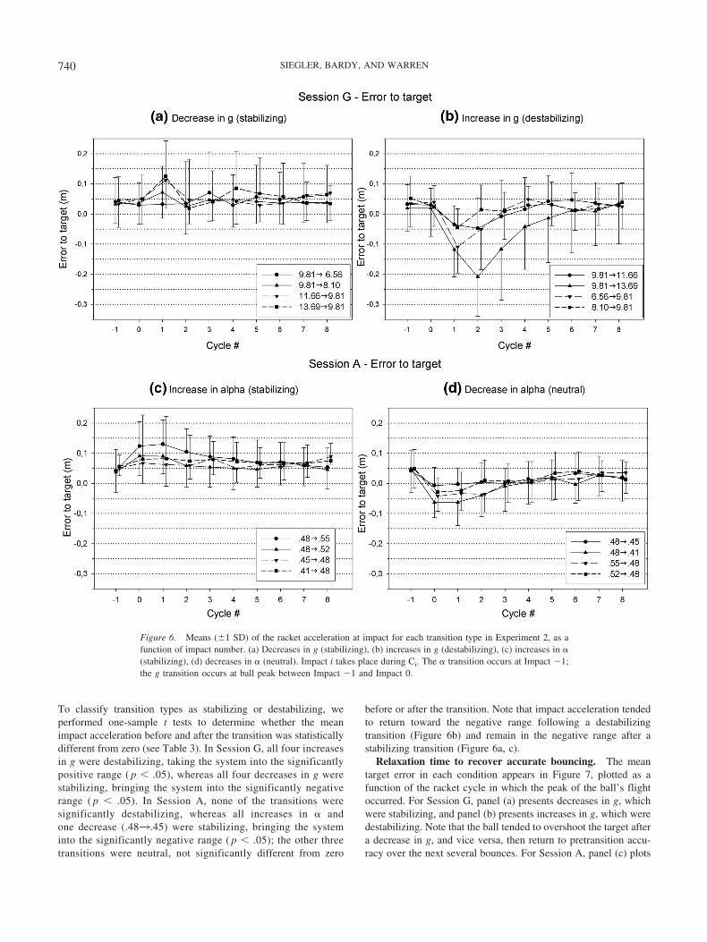
Relaxation time to recover accurate bouncing. The meantarget error in each condition appears in Figure 7, plotted as afunction of the racket cycle in which the peak of the ball’s flightoccurred. For Session G, panel (a) presents decreases in g, whichwere stabilizing, and panel (b) presents increases in g, which weredestabilizing. Note that the ball tended to overshoot the target aftera decrease in g, and vice versa, then return to pretransition accu-racy over the next several bounces. For Session A, panel (c) plots

Figure 6. Means (1 SD) of the racket acceleration at impact for each transition type in Experiment 2, as afunction of impact number. (a) Decreases in g (stabilizing), (b) increases in g (destabilizing), (c) increases in �(stabilizing), (d) decreases in � (neutral). Impact i takes place during Ci. The � transition occurs at Impact �1;the g transition occurs at ball peak between Impact �1 and Impact 0.


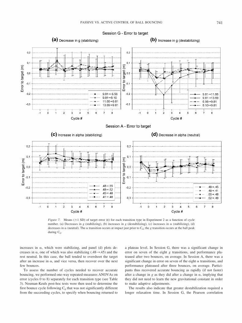
increases in �, which were stabilizing, and panel (d) plots de-creases in �, one of which was also stabilizing (.483.45) and therest neutral. In this case, the ball tended to overshoot the targetafter an increase in �, and vice versa, then recover over the nextfew bounces.

To assess the number of cycles needed to recover accuratebouncing, we performed one-way repeated-measures ANOVAs onerror (cycles 0 to 8) separately for each transition type (see Table3). Neuman-Keuls post-hoc tests were then used to determine thefirst bounce cycle following C0 that was not significantly differentfrom the succeeding cycles, to specify when bouncing returned to

a plateau level. In Session G, there was a significant change inerror on seven of the eight g transitions, and performance pla-teaued after two bounces, on average. In Session A, there was asignificant change in error on seven of the eight � transitions, andperformance plateaued after three bounces, on average. Partici-pants thus recovered accurate bouncing as rapidly (if not faster)after a change in g as they did after a change in �, implying thatthey did not need to learn the new gravitational constant in orderto make adaptive adjustments.

The results also indicate that greater destabilization required alonger relaxation time. In Session G, the Pearson correlation

Figure 7. Means (1 SD) of target error (ε) for each transition type in Experiment 2 as a function of cyclenumber. (a) Decreases in g (stabilizing), (b) increases in g (destabilizing), (c) increases in � (stabilizing), (d)decreases in � (neutral). The � transition occurs at impact just prior to C0; the g transition occurs at the ball peakduring C0.


between the first post-transition impact acceleration and the num-ber of bounces to plateau was r � .77. In Session A, the correlationwas only r � .26, reflecting the absence of destabilization and thenarrow range of impact accelerations.

Racket adjustments. To test active and passive stabilization,we examined racket adjustments following the transition. To nor-malize racket motion across conditions, we first determined refer-ence values of racket period by averaging the three pretransitioncycles (C�3 to C�1), and then computed ratios of racket periodover the reference value for racket cycles C�1 to C8. A ratio of 1.0indicates that a cycle period was equal to the pretransition refer-ence value, and a ratio greater than 1.0 indicates it was larger than

the reference value. This computation was repeated for racketamplitude.

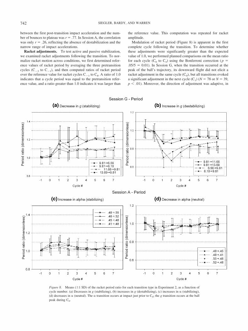
Modulation of racket period (Figure 8) is apparent in the firstcomplete cycle following the transition. To determine whetherthese adjustments were significantly greater than the expectedvalue of 1.0, we performed planned comparisons on the mean ratiofor each cycle (C0 to C4) using the Bonferroni correction ( p �.05/5 � 0.01). In Session G, when the transition occurred at thepeak of the ball’s trajectory, its downward flight did not elicit aracket adjustment in the same cycle (C0), but all transitions evokeda significant adjustment in the next cycle (C1) (N � 78 or N � 39,p � .01). Moreover, the direction of adjustment was adaptive, in

Figure 8. Means (1 SD) of the racket period ratio for each transition type in Experiment 2, as a function ofcycle number. (a) Decreases in g (stabilizing), (b) increases in g (destabilizing), (c) increases in � (stabilizing),(d) decreases in � (neutral). The � transition occurs at impact just prior to C0; the g transition occurs at the ballpeak during C0.


that racket period increased with a decrease in g (Figure 8a), andvice versa (Figure 8b). In Session A, when the transition occurredat impact, the ball’s complete flight was sufficient to elicit anadjustment in the same cycle (C0) for all transition types (N � 78or N � 39, p � .01). Again, the direction of adjustment wasadaptive, in that racket period increased with an increase in �(Figure 8c), and vice versa (Figure 8d). Importantly, these racketadjustments occurred not only after destabilizing transitions (Fig-ure 8a), but also after stabilizing transitions (Figure 8b, c) andneutral ones (Figure 8d) as well. Thus, participants rapidly andadaptively adjusted the period of the first complete racket cycleafter a transition, whether it destabilized the system or not.

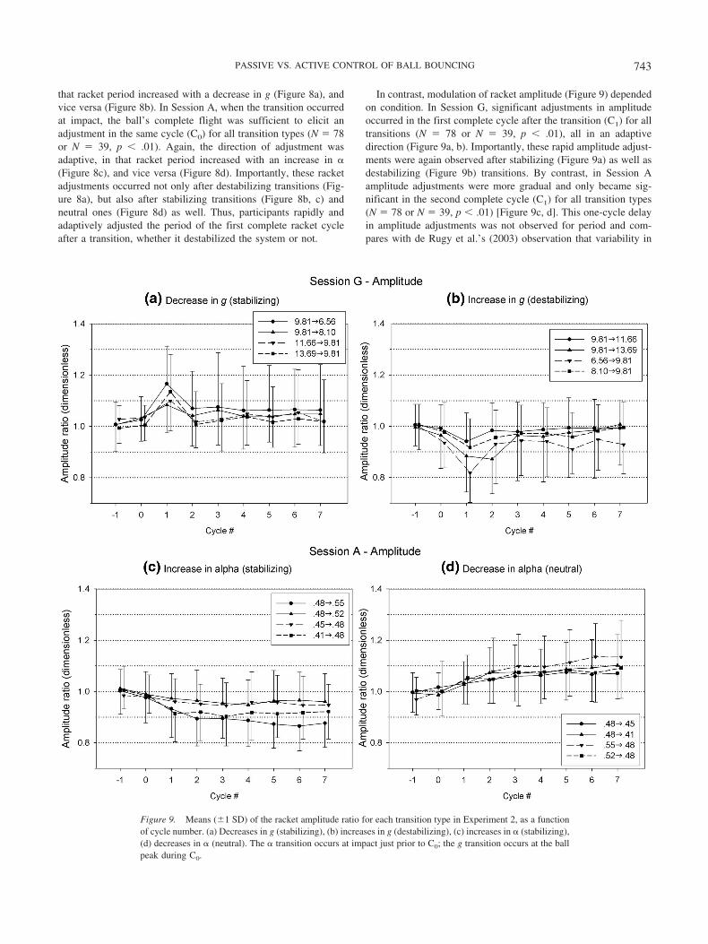
In contrast, modulation of racket amplitude (Figure 9) dependedon condition. In Session G, significant adjustments in amplitudeoccurred in the first complete cycle after the transition (C1) for alltransitions (N � 78 or N � 39, p � .01), all in an adaptivedirection (Figure 9a, b). Importantly, these rapid amplitude adjust-ments were again observed after stabilizing (Figure 9a) as well asdestabilizing (Figure 9b) transitions. By contrast, in Session Aamplitude adjustments were more gradual and only became sig-nificant in the second complete cycle (C1) for all transition types(N � 78 or N � 39, p � .01) [Figure 9c, d]. This one-cycle delayin amplitude adjustments was not observed for period and com-pares with de Rugy et al.’s (2003) observation that variability in

Figure 9. Means (1 SD) of the racket amplitude ratio for each transition type in Experiment 2, as a functionof cycle number. (a) Decreases in g (stabilizing), (b) increases in g (destabilizing), (c) increases in � (stabilizing),(d) decreases in � (neutral). The � transition occurs at impact just prior to C0; the g transition occurs at the ballpeak during C0.


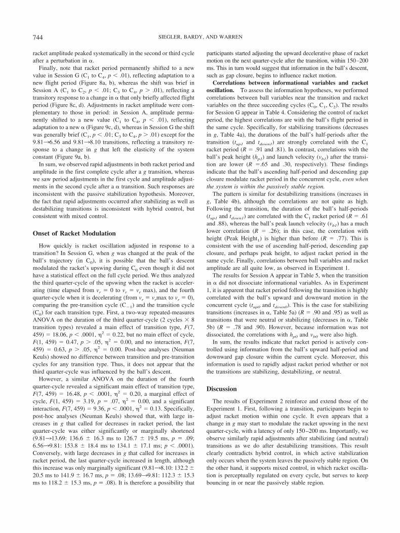
racket amplitude peaked systematically in the second or third cycleafter a perturbation in �.

Finally, note that racket period permanently shifted to a newvalue in Session G (C1 to C4, p � .01), reflecting adaptation to anew flight period (Figure 8a, b), whereas the shift was brief inSession A (C1 to C2, p � .01; C3 to C4, p � .01), reflecting atransitory response to a change in � that only briefly affected flightperiod (Figure 8c, d). Adjustments in racket amplitude were com-plementary to those in period: in Session A, amplitude perma-nently shifted to a new value (C1 to C4, p � .01), reflectingadaptation to a new � (Figure 9c, d), whereas in Session G the shiftwas generally brief (C1, p � .01; C3 to C4, p � .01) except for the9.8136.56 and 9.8138.10 transitions, reflecting a transitory re-sponse to a change in g that left the elasticity of the systemconstant (Figure 9a, b).

In sum, we observed rapid adjustments in both racket period andamplitude in the first complete cycle after a g transition, whereaswe saw period adjustments in the first cycle and amplitude adjust-ments in the second cycle after a � transition. Such responses areinconsistent with the passive stabilization hypothesis. Moreover,the fact that rapid adjustments occurred after stabilizing as well asdestabilizing transitions is inconsistent with hybrid control, butconsistent with mixed control.

Onset of Racket Modulation

How quickly is racket oscillation adjusted in response to atransition? In Session G, when g was changed at the peak of theball’s trajectory (in C0), it is possible that the ball’s descentmodulated the racket’s upswing during C0 even though it did nothave a statistical effect on the full cycle period. We thus analyzedthe third quarter-cycle of the upswing when the racket is acceler-ating (time elapsed from vr � 0 to vr � vr max), and the fourthquarter-cycle when it is decelerating (from vr � vrmax to vr � 0),comparing the pre-transition cycle (C�1) and the transition cycle(C0) for each transition type. First, a two-way repeated-measuresANOVA on the duration of the third quarter-cycle (2 cycles 8transition types) revealed a main effect of transition type, F(7,459) � 18.06, p � .0001, 2 � 0.22, but no main effect of cycle,F(1, 459) � 0.47, p � .05, 2 � 0.00, and no interaction, F(7,459) � 0.63, p � .05, 2 � 0.00. Post-hoc analyses (NeumanKeuls) showed no difference between transition and pre-transitioncycles for any transition type. Thus, it does not appear that thethird quarter-cycle was influenced by the ball’s descent.

However, a similar ANOVA on the duration of the fourthquarter-cycle revealed a significant main effect of transition type,F(7, 459) � 16.48, p � .0001, 2 � 0.20, a marginal effect ofcycle, F(1, 459) � 3.19, p � .07, 2 � 0.00, and a significantinteraction, F(7, 459) � 9.36, p � .0001, 2 � 0.13. Specifically,post-hoc analyses (Neuman Keuls) showed that, with large in-creases in g that called for decreases in racket period, the lastquarter-cycle was either significantly or marginally shortened(9.81313.69: 136.6 16.3 ms to 126.7 19.5 ms, p � .09;6.5639.81: 153.8 18.4 ms to 134.1 17.1 ms; p � .0001).Conversely, with large decreases in g that called for increases inracket period, the last quarter-cycle increased in length, althoughthis increase was only marginally significant (9.8138.10: 132.2 20.5 ms to 141.9 16.7 ms, p � .08; 13.6939.81: 112.3 15.3ms to 118.2 15.3 ms, p � .08). It is therefore a possibility that

participants started adjusting the upward decelerative phase of racketmotion on the next quarter-cycle after the transition, within 150–200ms. This in turn would suggest that information in the ball’s descent,such as gap closure, begins to influence racket motion.

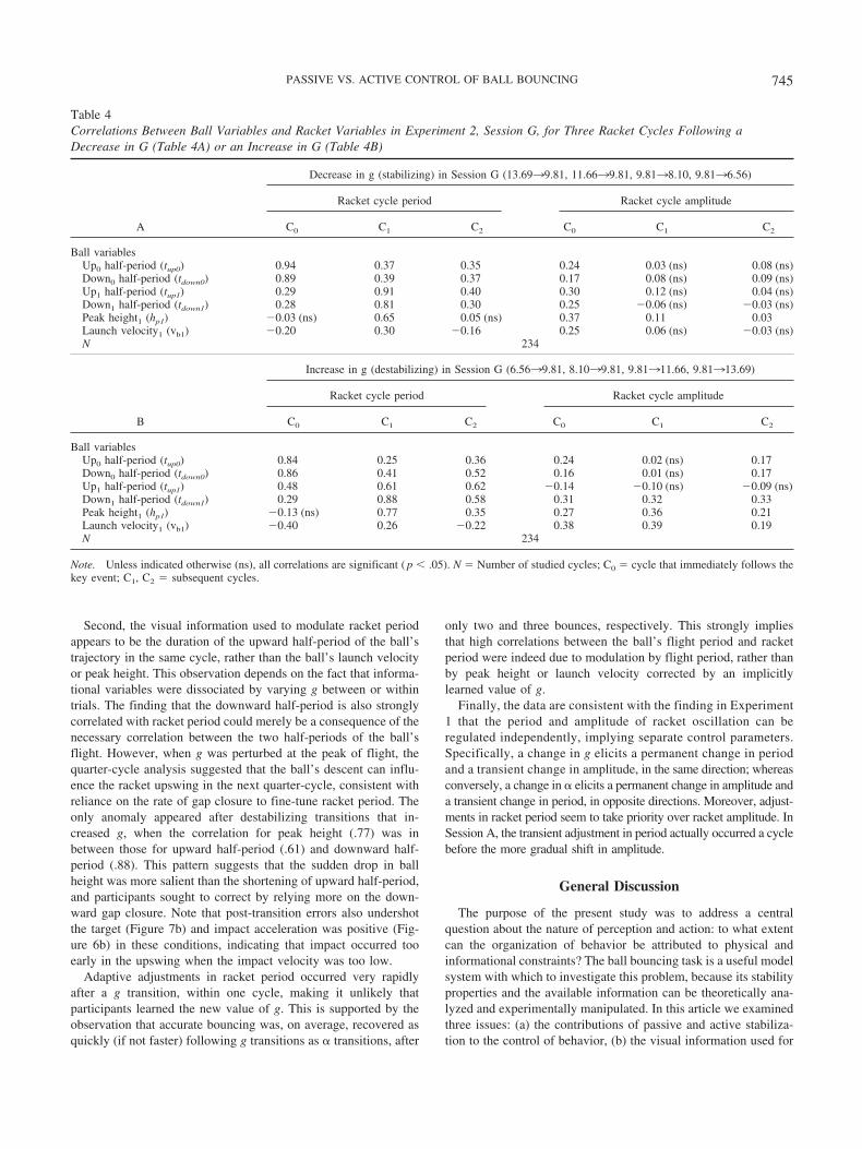
Correlations between informational variables and racketoscillation. To assess the information hypotheses, we performedcorrelations between ball variables near the transition and racketvariables on the three succeeding cycles (C0, C1, C2). The resultsfor Session G appear in Table 4. Considering the control of racketperiod, the highest correlations are with the ball’s flight period inthe same cycle. Specifically, for stabilizing transitions (decreasesin g, Table 4a), the durations of the ball’s half-periods after thetransition (tup1 and tdown1) are strongly correlated with the C1

racket period (R � .91 and .81). In contrast, correlations with theball’s peak height (hp1) and launch velocity (vb1) after the transi-tion are lower (R �.65 and .30, respectively). These findingsindicate that the ball’s ascending half-period and descending gapclosure modulate racket period in the concurrent cycle, even whenthe system is within the passively stable region.

The pattern is similar for destabilizing transitions (increases ing, Table 4b), although the correlations are not quite as high.Following the transition, the duration of the ball’s half-periods(tup1 and tdown1) are correlated with the C1 racket period (R � .61and .88), whereas the ball’s peak launch velocity (vb1) has a muchlower correlation (R � .26); in this case, the correlation withheight (Peak Height1) is higher than before (R � .77). This isconsistent with the use of ascending half-period, descending gapclosure, and perhaps peak height, to adjust racket period in thesame cycle. Finally, correlations between ball variables and racketamplitude are all quite low, as observed in Experiment 1.

The results for Session A appear in Table 5, when the transitionin � did not dissociate informational variables. As in Experiment1, it is apparent that racket period following the transition is highlycorrelated with the ball’s upward and downward motion in theconcurrent cycle (tup0 and tdown0). This is the case for stabilizingtransitions (increases in �, Table 5a) (R � .90 and .95) as well astransitions that were neutral or stabilizing (decreases in �, Table5b) (R � .78 and .90). However, because information was notdissociated, the correlations with hp0 and vb0 were also high.

In sum, the results indicate that racket period is actively con-trolled using information from the ball’s upward half-period anddownward gap closure within the current cycle. Moreover, thisinformation is used to rapidly adjust racket period whether or notthe transitions are stabilizing, destabilizing, or neutral.

Discussion

The results of Experiment 2 reinforce and extend those of theExperiment 1. First, following a transition, participants begin toadjust racket motion within one cycle. It even appears that achange in g may start to modulate the racket upswing in the nextquarter-cycle, with a latency of only 150–200 ms. Importantly, weobserve similarly rapid adjustments after stabilizing (and neutral)transitions as we do after destabilizing transitions. This resultclearly contradicts hybrid control, in which active stabilizationonly occurs when the system leaves the passively stable region. Onthe other hand, it supports mixed control, in which racket oscilla-tion is perceptually regulated on every cycle, but serves to keepbouncing in or near the passively stable region.


Second, the visual information used to modulate racket periodappears to be the duration of the upward half-period of the ball’strajectory in the same cycle, rather than the ball’s launch velocityor peak height. This observation depends on the fact that informa-tional variables were dissociated by varying g between or withintrials. The finding that the downward half-period is also stronglycorrelated with racket period could merely be a consequence of thenecessary correlation between the two half-periods of the ball’sflight. However, when g was perturbed at the peak of flight, thequarter-cycle analysis suggested that the ball’s descent can influ-ence the racket upswing in the next quarter-cycle, consistent withreliance on the rate of gap closure to fine-tune racket period. Theonly anomaly appeared after destabilizing transitions that in-creased g, when the correlation for peak height (.77) was inbetween those for upward half-period (.61) and downward half-period (.88). This pattern suggests that the sudden drop in ballheight was more salient than the shortening of upward half-period,and participants sought to correct by relying more on the down-ward gap closure. Note that post-transition errors also undershotthe target (Figure 7b) and impact acceleration was positive (Fig-ure 6b) in these conditions, indicating that impact occurred tooearly in the upswing when the impact velocity was too low.

Adaptive adjustments in racket period occurred very rapidlyafter a g transition, within one cycle, making it unlikely thatparticipants learned the new value of g. This is supported by theobservation that accurate bouncing was, on average, recovered asquickly (if not faster) following g transitions as � transitions, after

only two and three bounces, respectively. This strongly impliesthat high correlations between the ball’s flight period and racketperiod were indeed due to modulation by flight period, rather thanby peak height or launch velocity corrected by an implicitlylearned value of g.

Finally, the data are consistent with the finding in Experiment1 that the period and amplitude of racket oscillation can beregulated independently, implying separate control parameters.Specifically, a change in g elicits a permanent change in periodand a transient change in amplitude, in the same direction; whereasconversely, a change in � elicits a permanent change in amplitude anda transient change in period, in opposite directions. Moreover, adjust-ments in racket period seem to take priority over racket amplitude. InSession A, the transient adjustment in period actually occurred a cyclebefore the more gradual shift in amplitude.

General Discussion

The purpose of the present study was to address a centralquestion about the nature of perception and action: to what extentcan the organization of behavior be attributed to physical andinformational constraints? The ball bouncing task is a useful modelsystem with which to investigate this problem, because its stabilityproperties and the available information can be theoretically ana-lyzed and experimentally manipulated. In this article we examinedthree issues: (a) the contributions of passive and active stabiliza-tion to the control of behavior, (b) the visual information used for

Table 4Correlations Between Ball Variables and Racket Variables in Experiment 2, Session G, for Three Racket Cycles Following aDecrease in G (Table 4A) or an Increase in G (Table 4B)

A

Decrease in g (stabilizing) in Session G (13.6939.81, 11.6639.81, 9.8138.10, 9.8136.56)


C0 C1 C2 C0 C1 C2

Ball variablesUp0 half-period (tup0) 0.94 0.37 0.35 0.24 0.03 (ns) 0.08 (ns)Down0 half-period (tdown0) 0.89 0.39 0.37 0.17 0.08 (ns) 0.09 (ns)Up1 half-period (tup1) 0.29 0.91 0.40 0.30 0.12 (ns) 0.04 (ns)Down1 half-period (tdown1) 0.28 0.81 0.30 0.25 �0.06 (ns) �0.03 (ns)Peak height1 (hp1) �0.03 (ns) 0.65 0.05 (ns) 0.37 0.11 0.03Launch velocity1 (vb1) �0.20 0.30 �0.16 0.25 0.06 (ns) �0.03 (ns)N 234

B

Increase in g (destabilizing) in Session G (6.5639.81, 8.1039.81, 9.81311.66, 9.81313.69)


C0 C1 C2 C0 C1 C2

Ball variablesUp0 half-period (tup0) 0.84 0.25 0.36 0.24 0.02 (ns) 0.17Down0 half-period (tdown0) 0.86 0.41 0.52 0.16 0.01 (ns) 0.17Up1 half-period (tup1) 0.48 0.61 0.62 �0.14 �0.10 (ns) �0.09 (ns)Down1 half-period (tdown1) 0.29 0.88 0.58 0.31 0.32 0.33Peak height1 (hp1) �0.13 (ns) 0.77 0.35 0.27 0.36 0.21Launch velocity1 (vb1) �0.40 0.26 �0.22 0.38 0.39 0.19N 234

Note. Unless indicated otherwise (ns), all correlations are significant ( p � .05). N � Number of studied cycles; C0 � cycle that immediately follows thekey event; C1, C2 � subsequent cycles.


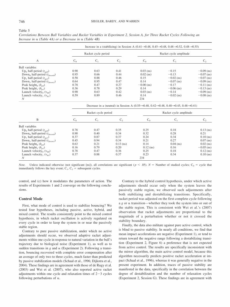
control, and (c) how it modulates the parameters of action. Theresults of Experiments 1 and 2 converge on the following conclu-sions.

Control Mode

First, what mode of control is used to stabilize bouncing? Wetested four hypotheses, including passive, active, hybrid, andmixed control. The results consistently point to the mixed controlhypothesis, in which racket oscillation is actively regulated onevery cycle in order to keep the system in or near the passivelystable region.

Contrary to pure passive stabilization, under which no activeadjustments should occur, we observed adaptive racket adjust-ments within one cycle in response to natural variation in the ball’strajectory due to biological noise (Experiment 1), as well as tosudden transitions in g and � (Experiment 2). Following a transi-tion, bouncing recovered with complete error compensation afteran average of only two to three cycles, much faster than predictedby passive stabilization models (Schaal et al., 1996; Dijkstra et al.,2004). These findings are in agreement with those of de Rugy et al.(2003) and Wei et al. (2007), who also reported active racketadjustments within one cycle and relaxation times of 2�3 cyclesfollowing perturbations of �.

Contrary to the hybrid control hypothesis, under which activeadjustments should occur only when the system leaves thepassively stable region, we observed such adjustments afterboth stabilizing and destabilizing transitions. Specifically,racket period was adjusted on the first complete cycle followinga g or � transition—whether they took the system into or out ofthe stable region. This is consistent with Wei et al.’s (2007)observation that racket adjustments are proportional to themagnitude of a perturbation whether or not it crossed thestability boundary.

Finally, the data also militate against pure active control, whichis blind to passive stability. In nearly all conditions, we find thatmean impact accelerations are negative (Experiment 1), or tend toreturn toward the negative range following a destabilizing transi-tion (Experiment 2, Figure 6) a preference that is not expectedfrom active control. The results are specifically inconsistent withthe mirror algorithm, the main active control model, because thisalgorithm necessarily predicts positive racket acceleration at im-pact (Schaal et al., 1996), whereas it was generally negative in thepresent experiment. In addition, traces of passive stability aremanifested in the data, specifically in the correlation between thedegree of destabilization and the number of relaxation cycles(Experiment 2, Session G). These findings are in agreement with

Table 5Correlations Between Ball Variables and Racket Variables in Experiment 2, Session A, for Three Racket Cycles Following anIncrease in � (Table 4A) or a Decrease in � (Table 4B)

A

Increase in a (stabilizing) in Session A (0.4130.48, 0.4530.48, 0.4830.52, 0.4830.55)


C0 C1 C2 C0 C1 C2

Ball variablesUp0 half-period (tup0) 0.90 0.63 0.41 0.03 (ns) �0.15 �0.09 (ns)Down0 half-period (tdown0) 0.95 0.66 0.44 0.02 (ns) �0.13 �0.07 (ns)Up1 half-period (tup1) 0.58 0.88 0.46 0.15 �0.02 (ns) �0.07 (ns)Down1 half-period (tdown1) 0.64 0.95 0.47 0.14 �0.07 (ns) �0.09 (ns)Peak height0 (hp0) 0.78 0.47 0.27 �0.00 (ns) �0.17 �0.11 (ns)Peak height1 (hp1) 0.36 0.78 0.29 0.14 �0.06 (ns) �0.13 (ns)Launch velocity0 (vb0) 0.90 0.63 0.42 0.03 (ns) �0.14 �0.09 (ns)Launch velocity1 (vb1) 0.59 0.89 0.46 0.14 �0.02 (ns) �0.08 (ns)N 234

B

Decrease in a (neutral) in Session A (0.5530.48, 0.4230.48, 0.4830.45, 0.4830.41)


C0 C1 C2 C0 C1 C2

Ball variablesUp0 half-period (tup0) 0.78 0.47 0.35 0.25 0.18 0.13 (ns)Down0 half-period (tdown0) 0.90 0.40 0.34 0.32 0.28 0.21Up1 half-period (tup1) 0.37 0.87 0.37 0.24 0.34 0.10 (ns)Down1 half-period (tdown1) 0.45 0.94 0.34 0.21 0.27 0.07 (ns)Peak height0 (hp0) 0.63 0.21 0.13 (ns) 0.14 0.04 (ns) 0.02 (ns)Peak height1 (hp1) 0.16 0.79 0.20 0.12 (ns) 0.16 �0.05 (ns)Launch velocity0 (vb0) 0.78 0.47 0.36 0.25 0.18 0.12 (ns)Launch velocity1 (vb1) 0.37 0.88 0.37 0.23 0.34 0.10 (ns)N 234

Note. Unless indicated otherwise (not significant [ns]), all correlations are significant ( p � .05). N � Number of studied cycles; C0 � cycle thatimmediately follows the key event; C1, C2 � subsequent cycles.


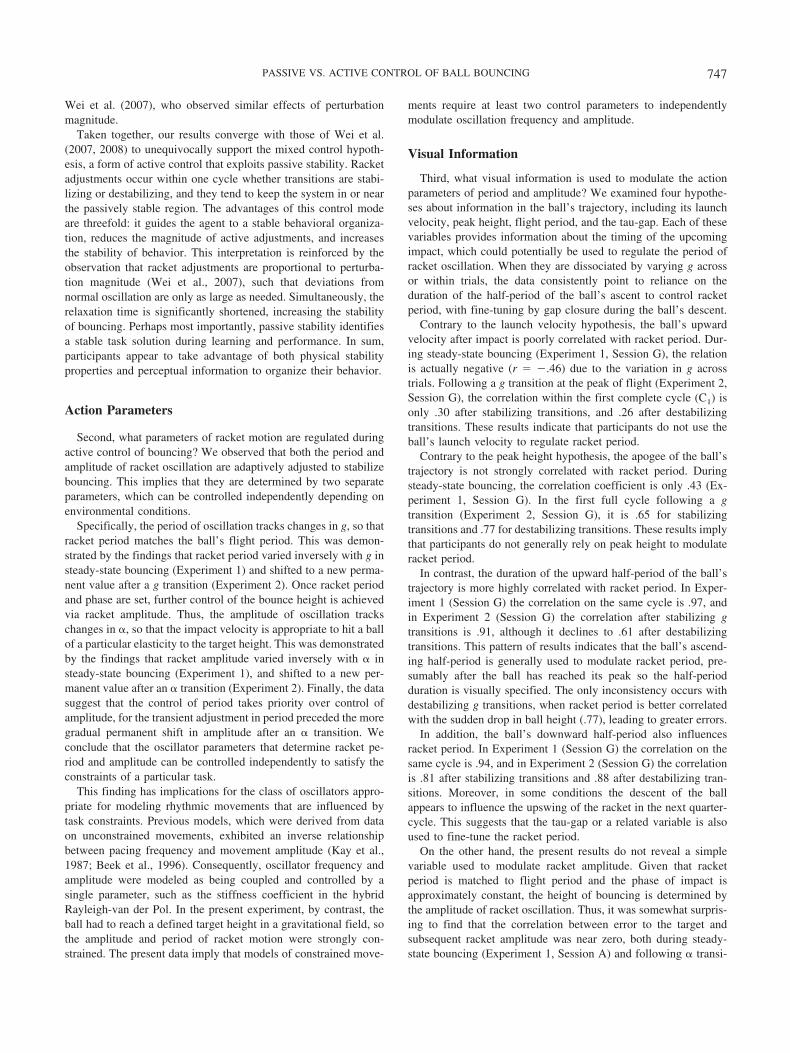
Wei et al. (2007), who observed similar effects of perturbationmagnitude.

Taken together, our results converge with those of Wei et al.(2007, 2008) to unequivocally support the mixed control hypoth-esis, a form of active control that exploits passive stability. Racketadjustments occur within one cycle whether transitions are stabi-lizing or destabilizing, and they tend to keep the system in or nearthe passively stable region. The advantages of this control modeare threefold: it guides the agent to a stable behavioral organiza-tion, reduces the magnitude of active adjustments, and increasesthe stability of behavior. This interpretation is reinforced by theobservation that racket adjustments are proportional to perturba-tion magnitude (Wei et al., 2007), such that deviations fromnormal oscillation are only as large as needed. Simultaneously, therelaxation time is significantly shortened, increasing the stabilityof bouncing. Perhaps most importantly, passive stability identifiesa stable task solution during learning and performance. In sum,participants appear to take advantage of both physical stabilityproperties and perceptual information to organize their behavior.

Action Parameters

Second, what parameters of racket motion are regulated duringactive control of bouncing? We observed that both the period andamplitude of racket oscillation are adaptively adjusted to stabilizebouncing. This implies that they are determined by two separateparameters, which can be controlled independently depending onenvironmental conditions.

Specifically, the period of oscillation tracks changes in g, so thatracket period matches the ball’s flight period. This was demon-strated by the findings that racket period varied inversely with g insteady-state bouncing (Experiment 1) and shifted to a new perma-nent value after a g transition (Experiment 2). Once racket periodand phase are set, further control of the bounce height is achievedvia racket amplitude. Thus, the amplitude of oscillation trackschanges in �, so that the impact velocity is appropriate to hit a ballof a particular elasticity to the target height. This was demonstratedby the findings that racket amplitude varied inversely with � insteady-state bouncing (Experiment 1), and shifted to a new per-manent value after an � transition (Experiment 2). Finally, the datasuggest that the control of period takes priority over control ofamplitude, for the transient adjustment in period preceded the moregradual permanent shift in amplitude after an � transition. Weconclude that the oscillator parameters that determine racket pe-riod and amplitude can be controlled independently to satisfy theconstraints of a particular task.

This finding has implications for the class of oscillators appro-priate for modeling rhythmic movements that are influenced bytask constraints. Previous models, which were derived from dataon unconstrained movements, exhibited an inverse relationshipbetween pacing frequency and movement amplitude (Kay et al.,1987; Beek et al., 1996). Consequently, oscillator frequency andamplitude were modeled as being coupled and controlled by asingle parameter, such as the stiffness coefficient in the hybridRayleigh-van der Pol. In the present experiment, by contrast, theball had to reach a defined target height in a gravitational field, sothe amplitude and period of racket motion were strongly con-strained. The present data imply that models of constrained move-

ments require at least two control parameters to independentlymodulate oscillation frequency and amplitude.

Visual Information

Third, what visual information is used to modulate the actionparameters of period and amplitude? We examined four hypothe-ses about information in the ball’s trajectory, including its launchvelocity, peak height, flight period, and the tau-gap. Each of thesevariables provides information about the timing of the upcomingimpact, which could potentially be used to regulate the period ofracket oscillation. When they are dissociated by varying g acrossor within trials, the data consistently point to reliance on theduration of the half-period of the ball’s ascent to control racketperiod, with fine-tuning by gap closure during the ball’s descent.

Contrary to the launch velocity hypothesis, the ball’s upwardvelocity after impact is poorly correlated with racket period. Dur-ing steady-state bouncing (Experiment 1, Session G), the relationis actually negative (r � �.46) due to the variation in g acrosstrials. Following a g transition at the peak of flight (Experiment 2,Session G), the correlation within the first complete cycle (C1) isonly .30 after stabilizing transitions, and .26 after destabilizingtransitions. These results indicate that participants do not use theball’s launch velocity to regulate racket period.

Contrary to the peak height hypothesis, the apogee of the ball’strajectory is not strongly correlated with racket period. Duringsteady-state bouncing, the correlation coefficient is only .43 (Ex-periment 1, Session G). In the first full cycle following a gtransition (Experiment 2, Session G), it is .65 for stabilizingtransitions and .77 for destabilizing transitions. These results implythat participants do not generally rely on peak height to modulateracket period.

In contrast, the duration of the upward half-period of the ball’strajectory is more highly correlated with racket period. In Exper-iment 1 (Session G) the correlation on the same cycle is .97, andin Experiment 2 (Session G) the correlation after stabilizing gtransitions is .91, although it declines to .61 after destabilizingtransitions. This pattern of results indicates that the ball’s ascend-ing half-period is generally used to modulate racket period, pre-sumably after the ball has reached its peak so the half-periodduration is visually specified. The only inconsistency occurs withdestabilizing g transitions, when racket period is better correlatedwith the sudden drop in ball height (.77), leading to greater errors.

In addition, the ball’s downward half-period also influencesracket period. In Experiment 1 (Session G) the correlation on thesame cycle is .94, and in Experiment 2 (Session G) the correlationis .81 after stabilizing transitions and .88 after destabilizing tran-sitions. Moreover, in some conditions the descent of the ballappears to influence the upswing of the racket in the next quarter-cycle. This suggests that the tau-gap or a related variable is alsoused to fine-tune the racket period.

On the other hand, the present results do not reveal a simplevariable used to modulate racket amplitude. Given that racketperiod is matched to flight period and the phase of impact isapproximately constant, the height of bouncing is determined bythe amplitude of racket oscillation. Thus, it was somewhat surpris-ing to find that the correlation between error to the target andsubsequent racket amplitude was near zero, both during steady-state bouncing (Experiment 1, Session A) and following � transi-


tions (Experiment 2, Session A), when g was constant. This resultimplies that adjustments in racket amplitude are not based on theerror in a single bounce, but may adapt more gradually based onaverage error over several preceding bounces. Such an interpreta-tion is consistent with the gradual shift in racket amplitude overabout four cycles we observed following � transitions (Figure 9b).Given the level of biological noise in bouncing, this would avoidamplifying variable error while reducing constant error with ballsof different elasticity.

In sum, when informational variables are dissociated by varyingg, racket period is more strongly correlated with the ascendinghalf-period of the ball’s flight, rather than its launch velocity orpeak height. This is an elegant solution that simply maps the ball’supward half-period into the racket period, a relation that holdsindependent of the gravitational constant and thus does not requireknowledge of g. It also explains why our participants were able toadapt to sudden changes in g within a few cycles, whereas McIn-tyre et al.’s (2001) astronauts failed to do so after many trials. Inour bouncing task, participants had access to upward half-periodinformation that specified the required racket period withoutknowledge of g, whereas in their catching task the upward half-period information was unavailable, so action had to be recali-brated to a new value of g.

Putting these pieces together, the following account of theperception–action cycle in ball bouncing emerges. The bouncingtask involves coupling a limit-cycle racket oscillation to a periodicball trajectory. The physical coupling at impact yields the bounc-ing ball map with its passive stability properties. The informationalcoupling actively stabilizes bouncing cycle by cycle, while keep-ing the system near the passively stable region, in a form of mixedcontrol. In particular, the half-period of the ball’s upward flight isused to control the period of racket oscillation, perhaps by directlymodulating the oscillator’s stiffness parameter. In addition, a vari-able related to average bounce error probably modulates a param-eter that independently controls the amplitude of racket oscillation,on a slower time scale. De Rugy et al. (2003) proposed a prelim-inary version of such a model, which used the ball’s launchvelocity to reset the period of a neural half-center oscillator.Although this enabled the model to rapidly recover from � per-turbations, it would not adapt to changes in g as observed in thepresent data. Instead, the results suggest using the ball’s ascendinghalf-period to regulate a parameter governing the period of theracket oscillator.

Mixed control thus takes advantage of both physical andinformational constraints in order to realize a stable and adap-tive solution for a behavioral task. On the one hand, it serves toreduce adjustments and simplify control when compared to pureactive control, and on the other, it serves to reduce relaxationtime and increase stability when compared to pure passivecontrol. Such a mixed control mode may be a general strategyfor integrating passive stability with active stabilization inperception�action systems (Warren, 2006). For example, itappears to be manifested in the active control of passive dy-namic walking in legged robots (Collins, Ruina, Tedrake, &Wisse, 2005; Tedrake, Zhang, Fong, & Seung, 2004), balance ininverted pendulum systems (Foo, Kelso, & de Guzman, 2000;Schoner, 1991), and tasks such as infant bouncing in a “jollyjumper” (Goldfield, Kay, & Warren, 1993) or juggling a soccerball (Tlili, Mottet, Bupuy, & Pavis, 2004). In this manner,

actors take advantage of both physical stability properties andinformational variables in order to achieve stable and adaptivepatterns of behavior.

References

Beek, P. J., Rikkert, W. E. I., & van Wieringen, P. C. W. (1996). Limitcycle properties of rythmic forearm movements. Journal of Experimen-tal Psychology: Human Perception and Performance, 22, 1077–1092.

Bingham, G. P. (2004). A perceptually driven dynamical model of biman-ual rhythmic movement (and phase perception). Ecological Psychology,16, 45–53.

Bootsma, R. J., & Oudejans, R. R. D. (1993). Visual information abouttime-to-collision between two objects. Journal of Experimental Psychol-ogy: Human Perception and Performance, 19, 1041–1052.

Buhler, M., Koditschek, D. E., & Kindlmann, P. J. (1994). Planning andcontrol of robotic juggling and catching tasks. International Journal ofRobotics Research, 13, 101–118.

Collins, S., Ruina, A., Tedrake, R., & Wisse, M. (2005). Efficientbipedal robots based on passive-dynamic walkers. Science, 307,1082–1085.

de Rugy, A., Wei, K., Muller, H., & Sternad, D. (2003). Activelytracking ‘passive’ stability in a ball bouncing task. Brain Research,982, 64 –78.

Dijkstra, T. M. H., Katsumata, H., de Rugy, A., & Sternad, D. (2004). Thedialogue between data and model: Passive stability and relaxation be-havior in a ball bouncing task. Nonlinear Studies, 11, 319–344.

Foo, P., Kelso, J. A. S., & de Guzman, G. C. (2000). Functional stabili-zation of unstable fixed points: Human pole balancing using time-to-balance information. Journal of Experimental Psychology: Human Per-ception and Performance, 26, 1281–1297.

Gibson, J. J. (1979). The ecological approach to visual perception. Boston:Houghton Mifflin.

Goldfield, E. C., Kay, B. A., & Warren, W. H. (1993). Infant bouncing:The assembly and tuning of action systems. Child Development, 64,1128–1142.

Kay, B. A., Kelso, J. A., Saltzman, E. L., & Schoner, G. (1987). Space-timebehavior of single and bimanual rhythmical movements: Data and limitcycle model. Journal of Experimental Psychology: Human Perceptionand Performance, 13, 178–192.

Kay, B. A., & Warren, W. H. (2001). Coupling of posture and gait: Modelocking and parametric excitation. Biological Cybernetics, 85, 89–106.

Lee, D. N. (1976). A theory of visual control of braking based on infor-mation about time-to-collision. Perception, 5, 437–459.

McIntyre, J., Zago, M., Berthoz, A., & Lacquaniti, F. (2001). Does thebrain model Newton’s laws? Nature Neuroscience, 4, 693–694.

Morice, A., Siegler, I. A., & Bardy, B. G. (2008). Action-perceptionpatterns in virtual ball bouncing: Combating system latency and trackingfunctional validity. Journal of Neuroscience Methods, 169, 255–266.

Morice, A., Siegler, I. A., Bardy, B. G., & Warren, W. H. (2007). Learningnew perception-action solutions in virtual ball bouncing. ExperimentalBrain Research, 181, 249–265.

Schoner, G. (1991). Dynamic theory of action-perception patterns: The‘moving room’ paradigm. Biological Cybernetics, 64, 455–462.

Schaal, S., Atkeson, C. G., & Sternad, D. (1996). One-handed juggling: Adynamical approach to a rhythmic movement task. Journal of MotorBehavior, 28, 165–183.

Siegler, I., Mantel, B., Warren, W. H., & Bardy, B. (2003, August).Behavioral dynamics of a rhythmic ball-bouncing task. Paper presentedat the Progress in Motor Control IV, Caen, France.

Sternad, D., Duarte, M., Katsumata, H., & Schaal, S. (2001). Bouncing aball: Tuning into dynamic stability. Journal of Experimental Psychol-ogy: Human Perception and Performance, 27, 1163–1184.

Tedrake, R., Zhang, T. W., Fong, M., & Seung, H. S. (2004). Actuating a


simple 3D passive dynamic walker. IEEE International Conference onRobotics and Automation, 5, 4656–4661.

Tlili, M., Mottet, D., Dupuy, M.-A., & Pavis, B. (2004). Stability and phaselocking in human soccer juggling. Neuroscience Letters, 360, 45–48.

Warren, W. H. (2006). The dynamics of perception and action. Psycho-logical Review, 113, 358–389.

Wei, K., Dijkstra, T. M. H., & Sternad, D. (2007). Passive stability andactive control in a rhythmic task. Journal of Neurophysiology, 98,2633–2646.

Wei, K., Dijkstra, T. M. H., & Sternad, D. (2008). Stability and variability:Indicators for passive stability and active control in a rhythmic task.Journal of Neurophysiology, 99, 3027–3041.

Appendix A

Haptic Information

Assume that ball mass mb, coefficient of restitution �, andgravitational acceleration g are constant for given conditions, andthat contact with the racket occurs at a constant height (hc). Tocontrol the timing of the next impact, a key desideratum is theperiod of the ball’s flight (Tb) between impacts, or the time of itsdownward flight from the peak of the trajectory until it returns tothe contact height (tdown).

By the laws of motion for falling bodies, the ball’s ith flight iscompletely determined by its launch velocity (vi), and the resultingflight period Ti is given by

Ti �2vi

g. (A1)

Assuming mb �� mr, the ball’s launch velocity following impactcan be determined from its incident velocity prior to impact ui�1,by the change in momentum:

mbvi � �mb ui�1 � Fi�ti

vi � �ui�1 �Fi�ti

mb

(A2)

where � is the coefficient of restitution, and Fi is the force and �tithe duration of contact; note that the latter constitute the impulse ofimpact I � F�t. Substituting (2) into (1), we get

Ti �

2��ui�1 �Fi�ti

mb�

g. (A3)

Noting that ui � 1 is equal to the preceding launch velocity vi � 1

for the i � 1th flight, from (1) we obtain

ui�1 � vi�1 �gTi�1

2. (A4)

Finally, substituting (4) into (3) allows us to predict the currentflight period from the preceding flight period and the impactimpulse:

Ti � �Ti�1 �2Fi�ti

gmb(A5)

where �, mb, and g are constants.

Appendix B

Optical Information

(i) Launch velocity. By the laws of motion, the current velocityof a falling body is

v � vo � gt (B1)

Hence, on the ball’s ith flight its incident velocity at contact withthe racket (ui) is related to the downward flight time (tdown) fromthe peak height (where vo � 0) to the contact height,

ui � � gtdown (B2)

and rearranging,

tdown � �ui

g. (B3)

Given that the incident velocity is equal to the launch veloc-ity on that cycle (ui � �vi) and substituting into B3, we obtainthat the downward flight time is a function of the launchvelocity:

tdown �vi

g(B4)

or

Tb �2vb

g. (B5)

(ii) Peak height. By the laws of motion, the current height ofa falling body is

(Appendices continue)


hp � hc � vot �1

2gtdown

2. (B6)

Since vo � 0 at the peak height hp, rearranging we obtain that thedownward flight time is a function of peak height:

tdown � �2hp

g(B7)

or

Tb � 2�2hp

g. (B8)

(iii) Half-period. The duration of the upward half-period fromcontact to the peak of the flight (tup) is equal to that of thedownward half-period from peak to the next contact (tdown). Thus,the downward flight time is specified by the upward half-period:

tdown � tup (B9)

or

Tb � 2tup. (B10)

(iv) Tau-gap. Hitting the ball entails controlling the motion-gap between the ball and the racket. Lee (1976) suggests that timeunderlies the process of change of any motion-gap with the taufunction. Tau of a motion-gap is numerically equal to the ratio ofthe current size, x of the motion-gap to its current rate of closurex, i.e.:

�c � x/x. (B11)

Received August 1, 2008Revision received March 17, 2009

Accepted March 24, 2009 �
