Download - Pacific Orca Distribution Survey (PODS) conducted aboard ... · Pacific Orca Distribution Survey (PODS) ... Orca Distribution Survey (PODS), conducted aboard ... during the Pacific

June 2009

Pacific Orca Distribution Survey (PODS) conducted aboard the NOAA ship

McArthur II in March 2008

(STATE DEPT. CRUISE NO: 2008-019)

M. Bradley Hanson1, Dawn P. Noren1, Thomas F. Norris2, Candice K. Emmons1, Marla M. Holt1, Elizabeth Phillips3,4 and Jeannette E. Zamon4

1NOAA/NMFS/Northwest Fisheries Science Center 2725 Montlake Blvd. E

Seattle, WA 98112

2Bio-Waves Inc. 517 Cornish Dr.

Encinitas, CA 92024

3Oregon State University/CIMRS Pt. Adams Research Station

Hammond, OR 97121

4NOAA/NMFS/Northwest Fisheries Science Center Pt. Adams Research Station

Hammond, OR 97121

ii

Contents

List of Tables . . . . . . . . . . . . . . . . . . . . . . . . . . . . . . . . . . . . . . . . . . . . . . . . . . . . . . . . . . . . . . . . . ii

List of Figures . . . . . . . . . . . . . . . . . . . . . . . . . . . . . . . . . . . . . . . . . . . . . . . . . . . . . . . . . . . . . . . . ii

Introduction . . . . . . . . . . . . . . . . . . . . . . . . . . . . . . . . . . . . . . . . . . . . . . . . . . . . . . . . . . . . . . . . . . . 1

Survey Objectives . . . . . . . . . . . . . . . . . . . . . . . . . . . . . . . . . . . . . . . . . . . . . . . . . . . . . . . . . . . . . . 1

Study Area . . . . . . . . . . . . . . . . . . . . . . . . . . . . . . . . . . . . . . . . . . . . . . . . . . . . . . . . . . . . . . . . . . . 1

Itinerary . . . . . . . . . . . . . . . . . . . . . . . . . . . . . . . . . . . . . . . . . . . . . . . . . . . . . . . . . . . . . . . . . . . . . 1

Methods and Materials . . . . . . . . . . . . . . . . . . . . . . . . . . . . . . . . . . . . . . . . . . . . . . . . . . . . . . . . . . 2

Visual surveys . . . . . . . . . . . . . . . . . . . . . . . . . . . . . . . . . . . . . . . . . . . . . . . . . . . . . . . . . . 2

Acoustic Survey . . . . . . . . . . . . . . . . . . . . . . . . . . . . . . . . . . . . . . . . . . . . . . . . . . . . . . . . 3

Photo-Identification . . . . . . . . . . . . . . . . . . . . . . . . . . . . . . . . . . . . . . . . . . . . . . . . . . . . . 5

Biopsy Sampling . . . . . . . . . . . . . . . . . . . . . . . . . . . . . . . . . . . . . . . . . . . . . . . . . . . . . . . . 5

Prey remains collection . . . . . . . . . . . . . . . . . . . . . . . . . . . . . . . . . . . . . . . . . . . . . . . . . . . 6

Behavioral observations . . . . . . . . . . . . . .. . . . . . . . . . . . . . . . . . . . . . . . . . . . . . . . . . . . . 6

Oceanography . . . . . . . . . . . . . . . . . . . . . . . . . . . . . . . . . . . . . . . . . . . . . . . . . . . . . . . . . . 6

Results and Discussion . . . . . . . . . . . . . . . . . . . . . . . . . . . . . . . . . . . . . . . . . . . . . . . . . . . . . . . . . 7

Sightings and Search Effort – Cetaceans . . . . . . . . . . . . . . . . . . . . . . . . . . . . . . . . . . . . . . 7

Sightings and Search Effort – Sea Birds . . . . . . . . . . . . . . . . . . . . . . . . . . . . . . . . . . . . . . 7

Acoustics detections . . . . . . . . . . . . . . . . . . . . . . . . . . . . . . . . . . . . . . . . . . . . . . . . . . . . . . 7

Killer whale encounters . . . . . . . . . . . . . . . . . . . . . . . . . . . . . . . . . . . . . . . . . . . . . . . . . . . 8

Oceanography . . . . . . . . . . . . . . . . . . . . . . . . . . . . . . . . . . . . . . . . . . . . . . . . . . . . . . . . . . . 8

Acknowledgements . . . . . . . . . . . . . . . . . . . . . . . . . . . . . . . . . . . . . . . . . . . . . . . . . . . . . . . . . . . . . 8

Literature Cited . . . . . . . . . . . . . . . . . . . . . . . . . . . . . . . . . . . . . . . . . . . . . . . . . . . . . . . . . . . . . . . .9

Tables . . . . . . . . . . . . . . . . . . . . . . . . . . . . . . . . . . . . . . . . . . . . . . . . . . . . . . . . . . . . . . . . . . . . . . .10

Figures . . . . . . . . . . . . . . . . . . . . . . . . . . . . . . . . . . . . . . . . . . . . . . . . . . . . . . . . . . . . . . . . . . . . . . .18

iii

LIST OF TABLES

Table 1. Participating scientists . . . . . . . . . . . . . . . . . . . . . . . . . . . . . . . . . . . . . . . . . . . . . . . . . . . .10

Table 2. Visual survey effort summary . . . . . . . . . . . . . . . . . . . . . . . . . . . . . . . . . . . . . . . . . . . . . . 10

Table 3. Visual sightings summary – Cetaceans and pinnipeds . . .. . . . . . . . . . . . . . . . . . . . . . . . . 11

Table 4. Cetacean and pinniped sightings . . . . . . . . . . . . . . . . . . . . . . . . . . . . . . . . . . . . . . . . . . . 12

Table 5. Marine bird survey effort . . . . . . . . . . . . . . . . . . . . . . . . . . . . . . . . . . . . . . . . . . . . . . . . . 13

Table 6. Total counts of bird species . . . . . . . . . . . . . . . . . . . . . . . . . . . . . . . . . . . . . . . . . . . . . . . .14

Table 7. Acoustic detections of marine mammals . . . . . . . . . . . . . . . . . . . . . . . . . . . . . . . . . . . . .16

Table 8. Killer whale encounters . . . . . . . . . . . . . . . . . . . . . . . . . . . . . . . . . . . . . . . . . . . . . . . . . . . 16

Table 9. Summary of environmental data . . . . . . . . . . . . . . . . . . . . . . . . . . . . . . . . . . . . . . . . . . . . .16

Table 10. XBT deployment locations . . . . . . . . . . . . . . . . . . . . . . . . . . . . . . . . . . . . . . . . . . . . . . . .17

Table 11. CTD deployment locations . . . . . . . . . . . . . . . . . . . . . . . . . . . . . . . . . . . . . . . . . . . . . . . 17

LIST OF FIGURES

Figure 1. Cruise track . . . . . . . . . . . . . . . . . . . . . . . . . . . . . . . . . . . . . . . . . . . . . . . . . . . . . . . . . . . .18

Figure 2. Visual On and Off –effort monitoring of cetaceans . . . . . . . . . . . . . . . . . . . . . . . . . . . . .19

Figure 3. On and Off -effort sightings of cetaceans . . . . . . . . . . . . . . . . . . . . . . . . . . . . . . . . . . . . . 20

Figure 4. Acoustic detections of marine mammals . . . . . . . . . . . . . . . . . . . . . . . . . . . . . . . . . . . . . .21

Figure 5. XBT and CTD deployments . . . . . . . . . . . . . . . . . . . . . . . . . . . . . . . . . . . . . . . . . . . . . . 22

1

Pacific Orca Distribution Survey (PODS), conducted aboard the NOAA ship McArthur II in March 2008

M. Bradley Hanson, Dawn P. Noren, Thomas F. Norris, Candice K. Emmons, Marla M. Holt,

Elizabeth Phillips and Jeannette E. Zamon

Introduction

In 2001 the Southern resident killer whale (SRKW) population was petitioned for listing under

the Endangered Species Act (ESA). A series of workshops were held in 2003 and 2004 to

identify data gaps and risk factors associated with the 20% decline this population experienced in

the late 1990s. The primary data gap identified with this population was its winter distribution.

Although the population has been identifiable since 1976, only 12 documented sightings in the

winter in coastal waters existed in 2001, ranging form central California to the Queen Charlotte

Islands, British Columbia. With the 2005 listing of the population under the ESA, Critical

Habitat designation was required but in the initial designation none of the coastal U.S waters were

included due to a paucity of sighting data. In order to obtain location data to improve the Critical

Habitat designation, as well as obtain other information on behavior and prey selection, winter

cruises to locate SRKWs have been conducted annually from 2004, except for the year 2005 (no

sea days were allocated to this task in FY05). Here we report on the sighting and acoustic data

collected for killer whales and other marine mammal species and seabirds, as well as describe the

oceanographic data collected during the Pacific Ocean killer whale and cetaceans Distribution

survey, March 2008 (PODs 2008) conducted aboard the NOAA ship McArthur II.

Survey Objectives

The overall objective of this cruise was to locate southern resident killer whales (SRKWs) in

order to better document their winter range as well as improve our understanding of their

behavior and habitat use in these areas. In addition, other biological and oceanographic data were

collected to better characterize their environment. Other objectives included photo-identification,

behavioral observations, and acoustic study of sounds produced by other cetaceans in this area

during the winter.

Study Area

The survey tracklines for the project included the waters of the continental shelf from southern

Vancouver Island to central Oregon. This region is within the range of most of the documented

sightings of SRKW during the late March timeframe.

Itinerary

The cruise began on 17 March 2008 in Portland, Oregon and ended on 26 March 2008 in Seattle,

Washington. A set of predetermined tracklines were established prior to the survey to cover the

portion of the study area with the highest probability of encounter of SRKW based on previous

sightings. In general, the ship was to initially follow the tracklines from the mouth of the

Columbia River north to Grays Harbor, Washington. If no southern resident killer whales were

encountered the ship followed a set of tracklines south, potentially as far as central Oregon,

depending on weather and whale detections. The ship would then return north repeating these

tracklines. Tracklines were modified during the cruise due to weather or other considerations. In

addition, modifications were made by transiting directly to areas where recently reported

2

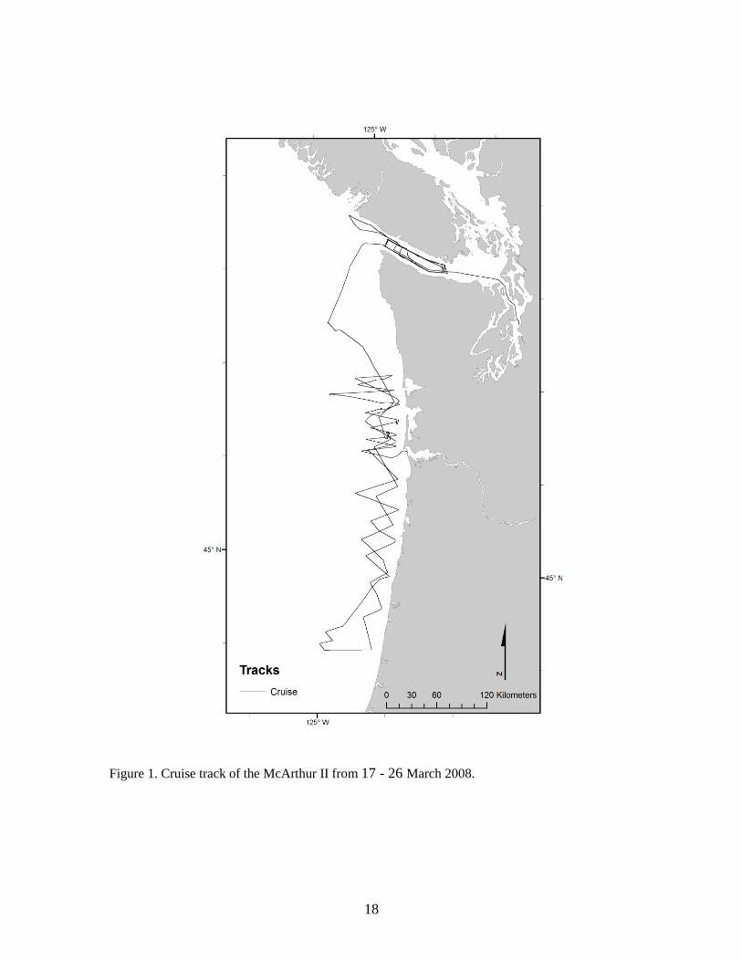
sightings of killer whales were likely to be southern resident killer whales. The final ship track is

shown in Figure 1.

Methods and Materials

Surveys were conducted for marine mammals and seabirds during this cruise. Two survey

methods for marine mammals were used, visual and acoustic. In addition, oceanographic data

were collected. Scientific Personnel that collected these data are listed in Table 1.

Visual Surveys

Marine Mammals

Line-transect survey methods were the primary visual survey method. This effort was consistent

with Southwest Fisheries Science Center’s approach for use in estimating abundance (Kinzey et

al. 2001). The McArthur II traveled at 9-10 knots (through the water) along the designated

trackline. A daily watch for marine mammals was maintained during daylight hours by scientific

observers on the flying bridge (approximately 0700 to 1800), except when the ship was stopped

to conduct other sampling operations, or when precluded by weather. A team of three observers

searched with 25x150 binoculars, 7X binoculars, and unaided eye. The two outboard observers

scanned from 10 degrees across the trackline to 90 degrees abeam with the Big Eyes. The

observers reported sighting angle using the azimuth incorporated into the binocular mount (this

azimuth was calibrated to zero at the beginning of the cruise). The recorder monitored the entire

180 degree field of view with 7x 50 binoculars and unaided eye. Sighting conditions, watch

effort, sightings, and other required information were entered into a computer, using the program

WinCruz (written by R. Holland, SWFSC), hooked up to the ship's GPS (for course, speed and

position information). Observers worked for 30 minutes at each of the three stations and rotated

through the three positions for a total of 1.5 hours on the flying bridge, with an hour break

between sets of rotations.

If weather (sea state, rain, or fog) precluded effective observations with the 25x binoculars, a two

observer watch (designated off-effort) was manned on either the flying bridge or bridge with

7x50 binoculars or unaided eye. The observers scanned with unaided eye and 7x50 binoculars for

marine mammals. Sighting conditions, watch effort, sightings, and other required information

were also entered into a computer by observers, using the program WinCruz (written by R.

Holland, SWFSC), hooked up to the ship's GPS (for course, speed and position information).

On sighting a marine mammal or other feature of biological interest, the marine mammal

observer team on watch occasionally requested the vessel be maneuvered to approach the

cetacean school or feature for investigation. During these occasions, the team went off-effort to

allow the ship to approach the group of marine mammals and make estimates of group size. For

killer whale sightings, behavioral state data were collected and photographs were taken. Weather

permitting, a small boat was deployed for biopsy, behavioral data collection, photographic and

other operations for killer whales. Depending on the duration and end location of the encounter

the trackline was generally re- intersected at the closet point.

3

Seabirds

Surveys of marine bird distribution were recorded by trained observers during daylight hours

when ship speed exceeded 2.5 m/s (5 knots). Two observers were on watch at all times during

survey effort. Observers went off-effort for meals and rest as necessary to avoid fatigue.

Observations began at dawn each morning. A primary observer counted and identified all flying

or sitting birds within a strip transect extending 300 m out from the bow to the beam of the ship

(90 arc), while the second observer recorded data and helped with identification and sightings of

birds close to the ship. During mild weather, observations were collected from the flying bridge

(deck height = 12.6 m) on the side of the vessel with the best viewing conditions for each survey

(e.g., no glare). In the event of precipitation exceeding a light drizzle, observations were collected

from the sheltered bridge wing in the lee of the wind (deck height 10.3 m).

Binoculars (8x magnification) were used to aid in counting and species identification. Data were

called out to the secondary observer who immediately entered them into a laptop computer

running the “SeeBird” data acquisition program v 2.3.0 (Southwest Fisheries Science Center, La

Jolla, CA). The computer was linked to GPS satellite data input so that each observation was

associated with a latitude/longitude position and time stamp. Behavior of seabirds was noted and

recorded (e.g. sitting, feeding, flying and flight direction, etc). Marine mammals, large

aggregations of seabirds, and rare species observed beyond the 300-m observation zone were also

recorded, using the SeeBird software’s capability to annotate distance outside of 300-m and the

“comment” feature in the software.

Acoustic survey - Two different types of acoustic monitoring systems were available during the

cruise, a dual towed array system and sonobuoys.

Towed Arrays - hydrophones

The towed array system consisted of 2 hydrophones arrays: a 2 element array (array A); and a 5

element array (array B). Array A consisted of 2 elements with 3.15 m spacing and approximately

330m of lead in cable. The 2 elements for array A had an effective (i.e. flat) frequency response

of 100 Hz – 40 kHz. Array A was the primary array deployed (i.e. day and night) during normal

survey mode. Array B consisted of 5 elements: two paired phones at either end with 3m spacing

between each element in the pair, and a single hydrophone near the middle (330 m from the end

pair and 130m from the first pair) for a total aperture of 660m (between the first and last pair).

The last element of array B consisted of a broad-band, high-frequency element with a flat

frequency response up to 200 kHz. Array B was intended to complement array A during

nighttime encounters with resident killer whales in order to improve tracking capabilities. Each

array was spooled on its own hydraulically powered winch for deployment and retrieval.

Usually, array A was deployed at lengths of 200-300m from the fantail of the ship, depending on

the bottom depth and other factors. Approximately 10 lbs of lead weight was attached to each

array approximately 180m from the end of the array to sink it to a suitable depth. Array B was

deployed with 200m of cable from the first pair of elements (for a total length of ~ 660m).

The deck cable was connected to the dry end of the array after deployment via a weather-proof

electronic connector. The deck cable led from the winch into the dry-lab where the array power

supply, signal conditioning, and signal processing, and signal recording system were located on

the McArthur II. Array A was powered by two 12V DC batteries using a differential power

(positive, negative & ground) configuration. Array B was powered by a 16V gel-cell.

4

Towed Arrays - Signal conditioning system

Six channels from both arrays (2 elements from array A, and the first 4 elements from array B)

were passed to a 6-channel low pass filter (Alligator Filter Tech. model AAF) set at a fixed 48

kHz corner frequency. The seventh channel (from hydrophone 5 of array B) was sent to a low-

pass filter with a corner frequency set at 96 kHz. The signal was then split between a National

Instruments 6062E DAQ card for (for high-frequency recordings) and a programmable band-pass

filter (Krohn-Hite model 3362) with a corner frequency set at 48 kHz. The high pass filter was

adjusted as needed between 500 Hz and 4 kHz (default set at 500Hz) and used to reduce any low-

frequency engine and flow noise. All seven channels (i.e. all hydrophones from both arrays)

were fed into a MOTU Traveler PC digital interface. The MOTU interface was used to digitize all

seven channels of array signals and then sent to ISHMAEL via a fire-wire cable.

Towed Arrays - Signal processing and recording system

One laptop was dedicated for running ISHMAEL sound localization and digital recording

software (developed by D. Mellinger, OSU-PMEL, Newport, OR). A second laptop was

dedicated to running Whaletrack II (developed by Glenn Gailey, TAMUG, TX). These two

computers were connected via a network connection to an Ethernet router which was used to pass

information from ISHMAEL to Whaletrack II (see Appendix II for setup procedures).

ISHMAEL was used to record acoustic data and process calls for localization. Generally, data

were sampled and recorded at 96 kHz for both arrays. Two-channels were recorded when array

A was deployed and 7 channels (2 from array A, and 5 from array B) when both arrays were

deployed. In some instances other sample rates and channels were recorded as needed.

Recordings were made continuously at 10 minute intervals with times with most start-times

aligned on the hour and every ten minutes after the hour.

Animal vocalizations were manually selected in ISHMAEL for localization by windowing the

signal with a pointing device (e.g. a trackball or touchpad). Depending on localization method

selected n ISHMAEL either a left-right ambiguous bearing, an un-ambiguous bearing, or a

relative location was estimated. All bearings and locations were estimated relative to the ship’s

location. Instantaneous estimates of locations were possible using a newly developed “crossed-

pair” localization method in ISHMAEL. The bearing or location estimate and additional

information were automatically passed to Whaletrack II via the network connection.

Whaletrack II was used to plot bearings and/or location estimates passed from ISHMAEL.

Whaletrack II also acquired and plotted ship position via a serial GPS connection. Ship track

history, current heading and speed as well as an estimated position of the array were calculated

and stored in an MSAccess database created by Whaletrack II. Information about effort, acoustic

contacts and settings of acoustic equipment (e.g. gain and filter cutoffs) were also recorded in

Whaletrack II.

Bearings plotted in Whaletrack II were used to estimate the animal’s location using a “sequential-

bearing fix” technique. This technique involved sequentially plotting several bearings to the

target while steadily moving past it. The locations of animal(s) were estimated visually by the

computer operator who subjectively assessed the point where the bearing lines intersect.

Bearings and estimated locations of animal calls were saved in a Whaletrack II database file.

Screen dumps of bearing and ship plots were occasionally saved.

5

Sonobuoy System

Type AN/SSQ-57B USN sonobuoys (effective audio frequency response 10 Hz – 20 kHz)

transmitting at various radio frequencies (164-167 MHz range) were deployed as conditions

warranted. Sonobuoys are self-contained units that automatically power-up upon contact with

water and transmit sounds via radio waves. All sonobuoys were set at 90m hydrophone

deployment depths and 8 hour operating life (auto-scuttle setting). The sonobuoy radio signals

were received by a mast mounted antennae connected to an ICOM IC-PCR1000 receiver that was

controlled through a PC-based software interface. Acoustic signals from the receiver were

recorded to a hard-drive using ISHMAEL and a NI 6062E DAQ card or the internal PC sound

card.

Towed Arrays - Monitoring

Array A was monitored 24/7 as the ship proceeded on the tracklines weather permitting and

except for oceanographic data collection during CTD deployment. The vessel slowed from

survey speed to approximately 3 knots at the midpoint of each line in order to provide improved

acoustic monitoring conditions. Array B was deployed primarily at night, to facilitate tracking,

and recovered in the morning. On occasion it was left out during the daytime. The array(s) were

retrieved during nighttime CTD operations (usually between 20:00 and 21:00) but were re-

deployed immediately afterwards. Only 2 channel recordings were made from Array A, even

when both arrays were deployed. This allowed faster computational times when obtaining

bearings and localizations.

A single visual observer on the flying bridge monitored the 2 element array aurally using a

headset at all times when the visual team was on effort. If a killer whale vocalization was

detected (or possibly detected), a member of bio-acoustics team was called to begin acoustics

monitoring in the acoustics lab and proceed to attempt to localize calls. If killer whale sounds

were detected at night, the bio-acoustician on watch would attempt to localize and track them

until the visual observers came on watch at daybreak.

If southern resident killer whales were detected, every effort was made to remain with these

animals for as long as possible. Visual sightings as well as acoustic data from the towed acoustic

array or sonobouys were used to track the whales. Behavioral data were collected during visual

observations, and if weather permitted, a small boat was deployed in order collect behavioral

data, predation event remains, and photographs.

Photo-ID Photographs of marine mammals were taken on an opportunistic basis. The animals

were either approached by the research vessel during normal survey operations, approached the

research vessel on their own, or were approached by a small boat. Photographs of individuals

were taken with digital 35 mm SLR cameras using 300 and 400 mm lenses for those species that

have photo-ID existing catalogs.

Biopsy Sampling - Biopsies for genetic analyses of killer whales were collected on an

opportunistic basis in U.S. and Canadian waters. Samples collected for killer whales were only

taken from small boats using the method outlined by Barrett-Leonard et al. (1996). For cetaceans

that approached within 10m to 30m of the bow of the McArthurII biopsy samples were collected

using a dart fired from a dart rifle (S. Claussen per.comm.).

Prey remains/fecal collection – Prey remains from predation events (scales, tissue) of marine

mammals and fecal samples were collected on an opportunistic basis. These samples were

6

collected from animals that were approached by the small boat using a long-handled (4-m)

fine-mesh net.

Behavioral Observations – Behavioral observations of marine mammals were taken on an

opportunistic basis. The animals to be observed were approached by the research vessel during

normal survey operations, approached the vessel on their own, or were approached by a small

boat. Observations recorded from the McArthurII included general behavioral state. During

small boat operations a focal follow approach was used that was similar to Ford and Ellis (2006).

Oceanography

Thermosalinograph Sampling

The ship’s Sea-bird Electronics Thermosalinograph (TSG) sampled surface water temperature

and salinity continuously during the entire cruise track. The data from the TSG and from a GPS

were continuously recorded by the ship's Scientific Computing System (SCS). The TSG

information was also used in the field by the oceanographer to record latitude, longitude, surface

water temperature, and salinity during expendable bathyothermograph (XBT) casts, surface water

sampling, and CTD casts.

Expendable Bathyothermographs (XBTs) Deployment and Surface Water sampling

Expendable bathyothermographs (XBTs) were deployed at 0900, 1200, and 1500 hours, and

surface water samples were collected at 0600, 0900, 1200, 1500, and 1800 hours local ship time,

and at other times, under the discretion of the Chief Scientist (e.g., surface water samples are also

taken every hour when in the presence of killer whales). For XBT deployments, Sippican Deep

Blue probes were used and data were transmitted to the Shipboard Environmental data

Acquisition System. After each XBT drop, a surface water sample for chlorophyll a analysis was

collected in a bucket deployed over the side of the ship. Immediately following bucket sampling,

a 50 ml sample of the water was filtered onto a 2.5 cm GF/F filter. All filters were wrapped in

foil, labeled, and stored frozen in Ziploc freezer bags until sample analysis, which occurred on the

ship within <1-2 weeks of collection. For extraction, the filters were placed in culture tubes with

8 ml of 90% (v/v) acetone and stored in the freezer for a minimum of 2 hours. The tubes were

then allowed to equilibrate with room temperature, and fluorescence was measured using a

Turner Designs 10-AU Digital Field Fluorometer.

CTD Casts

A CTD (conductivity-temperature-depth) station was occupied each evening one hour after

sunset, weather and sufficient depth permitting. In the event that a CTD cast was cancelled due to

inclement weather or because the ship was tracking killer whales, an XBT was also deployed

when the surface water sample was collected at 1800 hours. CTD data and seawater samples

were collected using a SeaBird 9/11+ CTD with a 12-place rosette and Niskin bottles. All casts

were to 1000m (depth permitting) with the descent rate set at 30 m/min for the first 100m of the

cast, then 60 m/min after that, including the upcast between bottles. Niskin bottle water samples

were collected at 12 standard depths (0, 10, 20, 30, 40, 50, 75, 100, 150, 200, 500, 1000) between

the surface and 1000 meters, or to within 10 m of the bottom. For each cast, water samples were

collected for chlorophyll a analysis at all depths to 200 m. Immediately following sampling, a 50

ml sample of the water was filtered onto a 2.5 cm GF/F filter. All filters were wrapped in foil,

labeled, and stored frozen in Ziploc freezer bags until sample analysis, which occurred on the

7

ship within <1-2 weeks of collection. Chlorophyll a extraction and analysis were conducted

using the same protocol as above. Water samples for salinity analysis were collected at 100, 500,

and 1000 m (or to within 10 m of bottom). Three additional salt samples were collected every

other day so that the depths sampled were 30 m, 100m, 150m, 200 m, 500 m, and 1000 m. Water

samples for salinity analysis were stored upright at ambient room temperature. Salinity samples

were processed within one month after the cruise at the University of Washington Marine

Chemistry Laboratory in Seattle. Water samples (approximately 40 ml) for nutrient analysis from

each of the 11 depths up to 500 m were transferred into pre-rinsed (10% HCl and H2O) vials and

frozen upright. Nutrient samples were processed within 1 year after the cruise, at the University

of Washington Marine Chemistry Laboratory in Seattle.

Results and Discussion

Search Effort and Sightings – Marine mammals

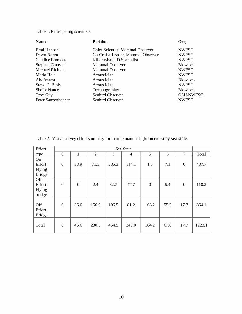
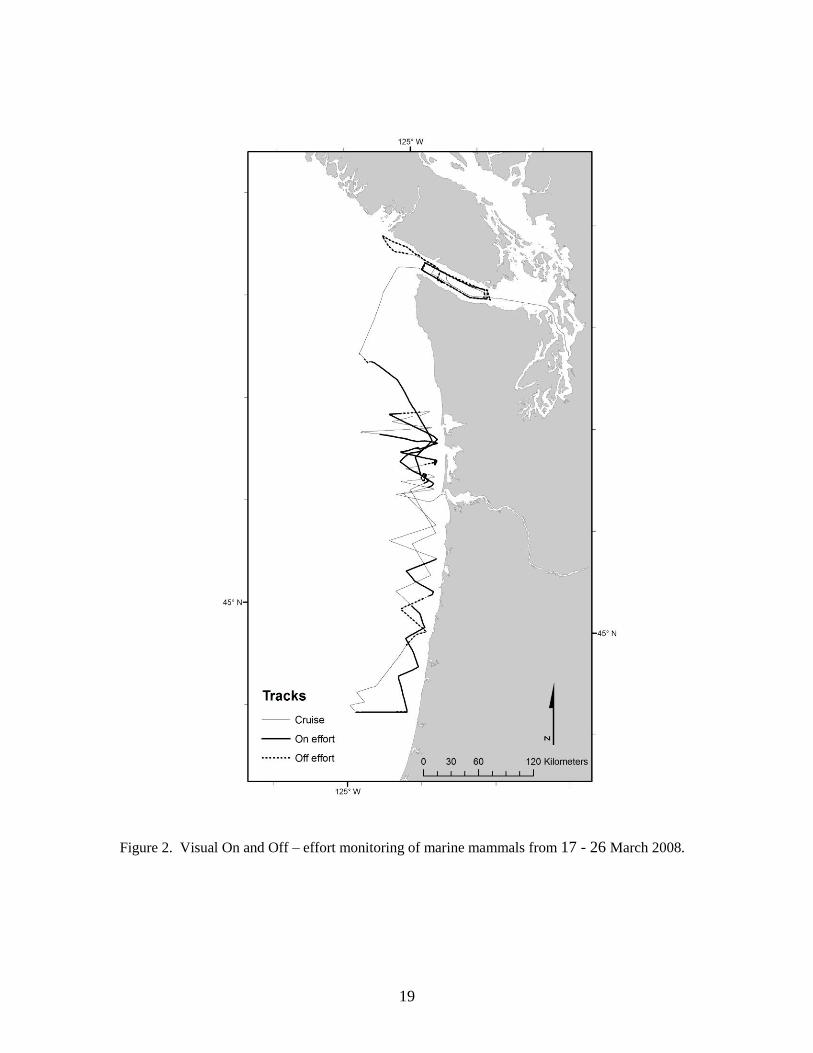
A total of 1223.1 km were surveyed in the study area during eight of the 10 total sea days,

yielding an average of 152.9 km/day (Table 2, Figure 2). However, only 487.7 km were

considered on-effort, and of the 735.4 km total off–effort, 118.2 km were conducted on the flying

bridge and 617.2 were conducted on the bridge. Survey efforts were hampered from 23-25

March due to inclement weather.

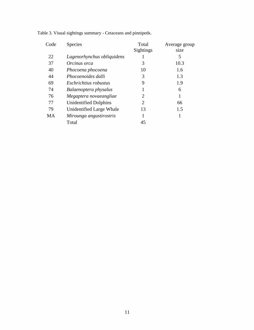
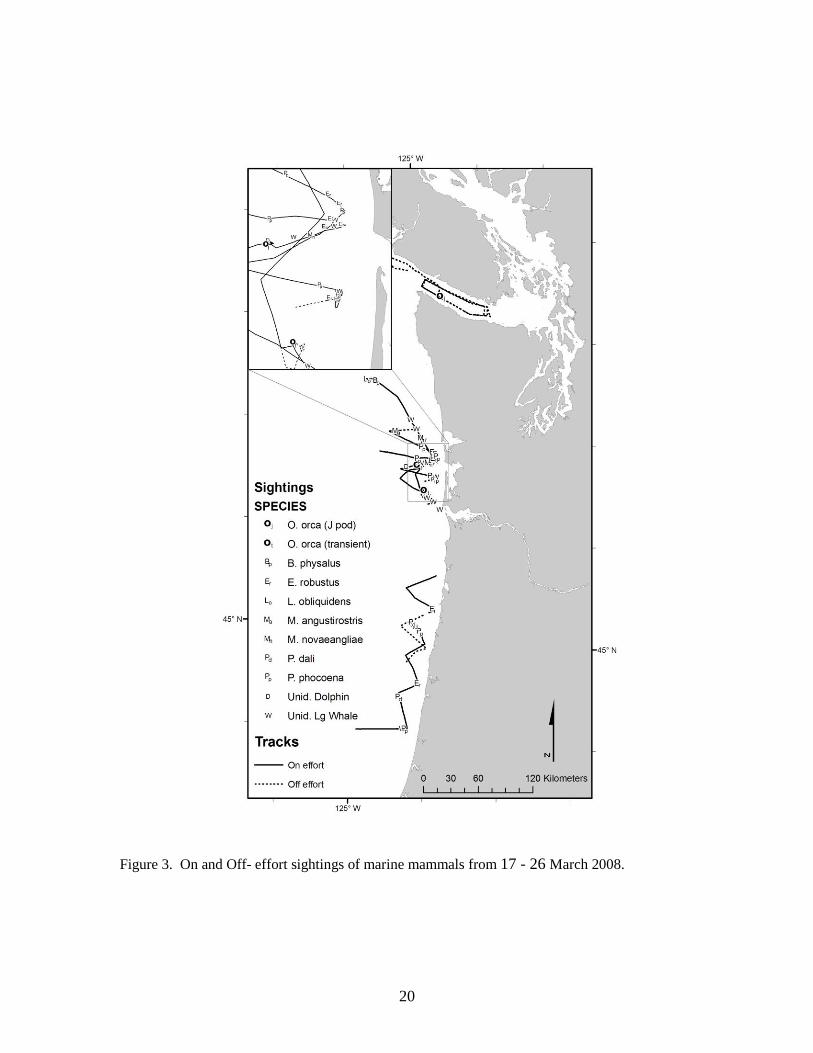
A total of 45 marine mammal sightings were made during all effort categories (Table 3). The

majority of sightings were made while on-effort (39) although a few were observed while off–

effort (6) (Table 4). Seven identifiable cetacean and one pinniped species were sighted (Figure

3). The most commonly sighted species were unidentified large whales, followed by harbor

porpoise (Phocoena phocoena) and gray whales (Eschrichtius robustus). Two groups of killer

whales (transients) were initially sighted without an acoustic cue (see Acoustics section). No

ship-based biopsy attempts were made. We collected one biopsy sample from southern resident

killer whales (J pod) encountered on 25 March in Canadian waters.

Search effort and sightings - Seabirds

A total of 931.7 kilometers of on-effort survey observations were collected between 18 Mar 2008

and 24 Mar 2008; total effort for each day is shown in Table 5. Observation conditions were

generally good: average Beaufort sea state was 3, and the Observing Condition factor, which is a

qualitative measure of the ability to detect small, fast-moving species such as phalaropes or

storm-petrels, was either Fair or Good for all surveys.

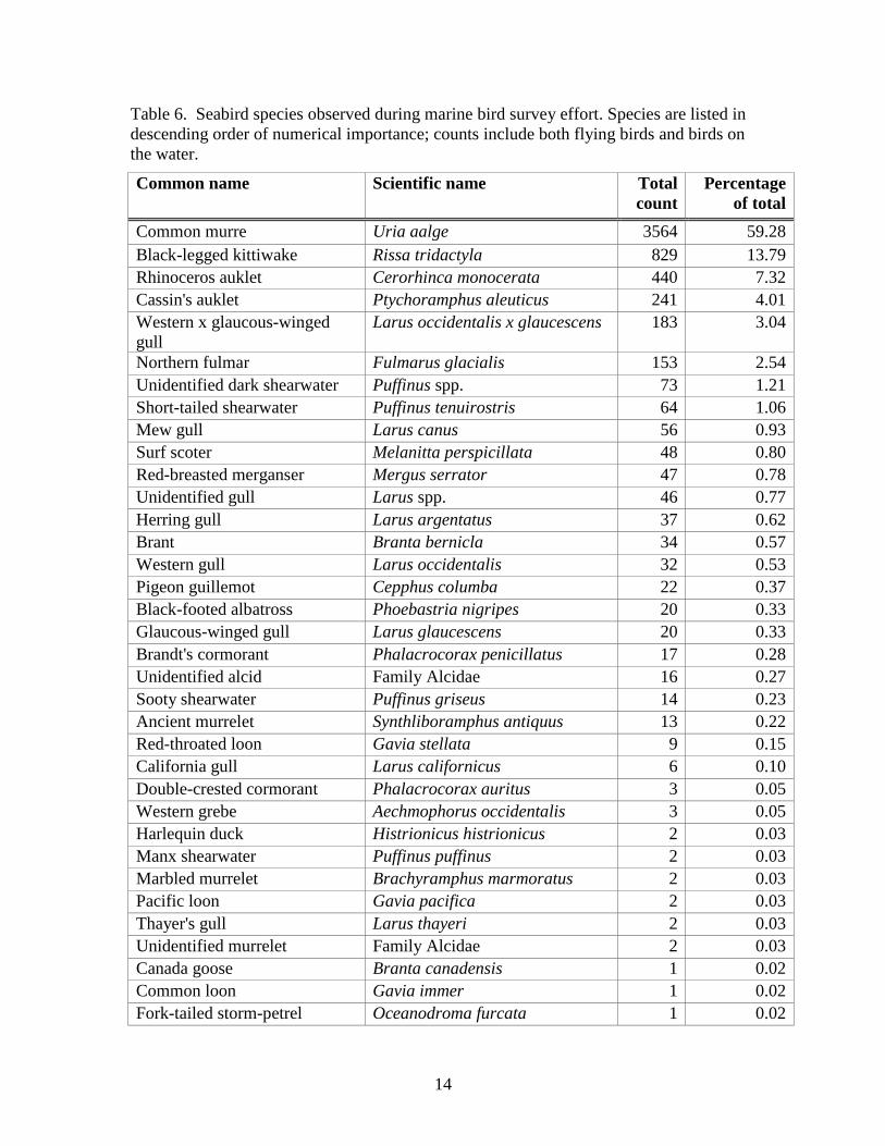
A total of 6,012 seabirds were observed and counted during on-effort transects (Table 6). Ninety

percent of all birds counted were from only six species: common murre (Uria aalge, 59.3%),

black-legged kittiwake (Rissa tridactyla, 13.8%), rhinoceros auklet (Cerorhinca monocerata,

7.3%), Cassin’s auklet (Ptychoramphus aleuticus, 4.0%), western-glaucous-winged hybrid gulls

(Larus occidentalis x glausescens, 3.0%), and northern fulmars (Fulmarus glacialis, 2.5%). The

observed species composition indicates an assemblage of primarily non-breeding late winter

migrants (e.g. kittiwakes) and resident breeding species (e.g. murres), as well as a few non-

breeding summer migrants (e.g. sooty shearwaters).

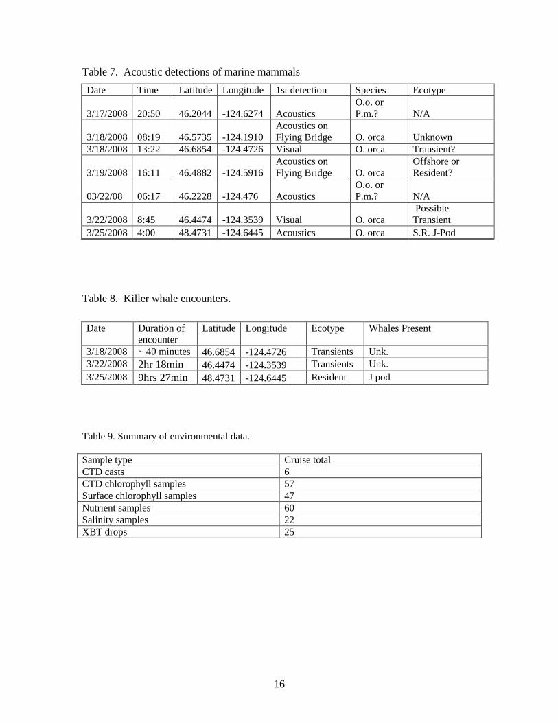
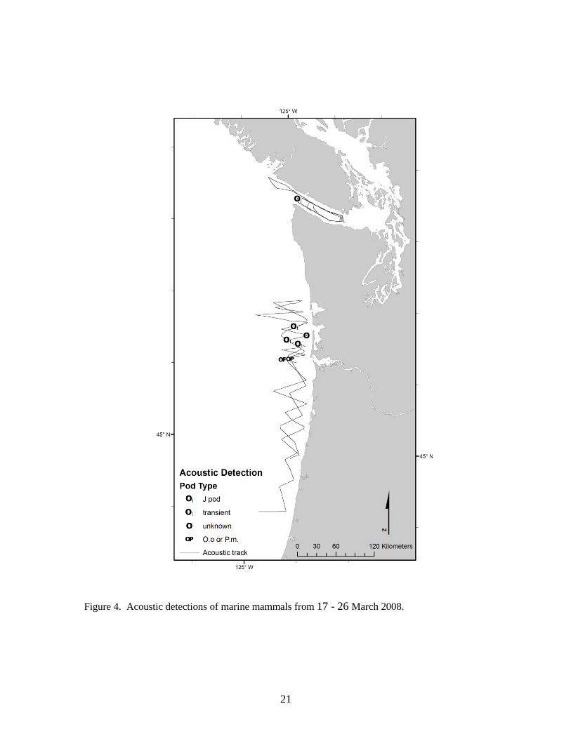
Acoustic detections

During the eight days at sea in the study area, the towed array system (i.e. at least one towed

array) was deployed and monitored for a total of 159 hours. Excluding the first and last sea days

8

(when partial days only were possible) average daily acoustic effort (day and night) was

approximately 21.1 hours per day. If the times the array had to be retrieved for the daily CTD

cast and inclement weather periods are excluded (~ 28 hrs) , the resulting 159 hour effort

represents approximately 95% of the time ‘available’ for conducting acoustic effort. All acoustic

data during on-effort period were digitally recorded to hard drives. There were no significant

malfunctions of the acoustic array or any related acoustic hardware. No sonobuoys were

deployed.

A total of seven acoustic detections were made during the cruise. All were attributed (or possibly

attributed) to killer whales although sperm whales (Physeter macrocephalus) could not be ruled

out (Table 7). Of these, four acoustic detections were visually confirmed, including a night-time

detection of the southern resident J-pod that was acoustically tracked until daylight when the pod

was visually located. Of those acoustic detections that were not visually confirmed, one (# 7) was

of a few faint killer whale calls that were not heard again. The two remaining detections (#1 and

#9) were clicks and could not be definitively attributed to killer whales in the field.

Killer whale encounters

Two of the three ecotype of killer whales found in the North Pacific Ocean, transients and

residents, were encountered during the cruise (Table 8). For the resident type, J pod from the

southern community was observed in U.S. and Canadian waters. We were able to conduct small

boat operations with this group of whales for several hours and one biopsy sample was collected.

No predation event or fecal samples were collected. We also encountered two groups of

transients, both off southern Washington.

Oceanography

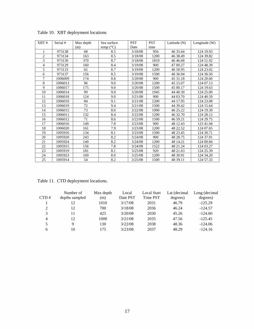
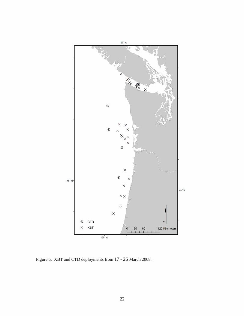
Twenty-five XBT deployments and six CTD deployments were made during the cruise (Table 9,

10, 11, Figure 5). Forty-seven surface chlorophyll samples, 57 CTD chlorophyll samples, 22

salinity samples, and 60 nutrient samples were collected.

Acknowledgements

This cruise report is dedicated to Stephen Claussen. We are grateful to the officers and crew of

the McArthur II for their support, and their expertise was essential to the success of this cruise.

The accomplishments of the cruise would not have been possible without the dedication and hard

work of the research team participants. Cruise logistics were assisted by NWFSC staff, including

Christel Martin, and Nick Adams and other staff from Vera Trainer’s program. We appreciate

the support and assistance of several colleagues at the SWFSC. Special thanks to Damon Holzer,

NWFSC for expert development of the figures. Marine mammal research in the U.S. was

conducted under NMFS Permit No. 782-1824-01 issued to the NWFSC and in Canada under

DFO Marine Mammal License 2008-03 and SARA License 84.

9

Literature Cited

Barrett-Lennard, L. G., T. G. Smith, and G. M. Ellis. 1996. A cetacean biopsy system

using lightweight pneumatic darts, and its effect on the behavior of killer whales.

Marine Mammal Science 12:14-27.

Ford, J.K.B., and Ellis, G.M. 2006. Selective foraging by fish-eating killer whales

Orcinus orca in British Columbia. Marine Ecology Progress Series 316: 185–199.

Kinzey, D., Gerrodette, T., Dizon, A., Perryman, W., Olson, P. and Rankin, S. 2001. Marine

Mammal Data Collected During a Survey in the Eastern Tropical Pacific Ocean Aboard

the NOAA Ships McArthur and David Starr Jordan, July 28 – December 09, 2000.

10

Table 1. Participating scientists.

Name1 Position Org

Brad Hanson Chief Scientist, Mammal Observer NWFSC

Dawn Noren Co-Cruise Leader, Mammal Observer NWFSC

Candice Emmons Killer whale ID Specialist NWFSC

Stephen Claussen Mammal Observer Biowaves

Michael Richlen Mammal Observer NWFSC

Marla Holt Acoustician NWFSC

Aly Azarra Acoustician Biowaves

Steve DeBlois Acoustician NWFSC

Shelly Nance Oceanographer Biowaves

Troy Guy Seabird Observer OSU/NWFSC

Peter Sanzenbacher Seabird Observer NWFSC

Table 2. Visual survey effort summary for marine mammals (kilometers) by sea state.

Effort

type

Sea State

0 1 2 3 4 5 6 7 Total

On

Effort

Flying

Bridge

0

38.9

71.3

285.3

114.1

1.0

7.1

0

487.7

Off

Effort

Flying

bridge

0

0

2.4

62.7

47.7

0

5.4

0

118.2

Off

Effort

Bridge

0

36.6

156.9

106.5

81.2

163.2

55.2

17.7

864.1

Total

0

45.6

230.5

454.5

243.0

164.2

67.6

17.7

1223.1

11

Table 3. Visual sightings summary - Cetaceans and pinnipeds.

Code Species Total

Sightings

Average group

size

22 Lagenorhynchus obliquidens 1 5

37 Orcinus orca 3 10.3

40 Phocoena phocoena 10 1.6

44 Phocoenoides dalli 3 1.3

69 Eschrichtius robustus 9 1.9

74 Balaenoptera physalus 1 6

76 Megaptera novaeangliae 2 1

77 Unidentified Dolphins 2 66

79 Unidentified Large Whale 13 1.5

MA Mirounga angustirostris 1 1

Total 45

12

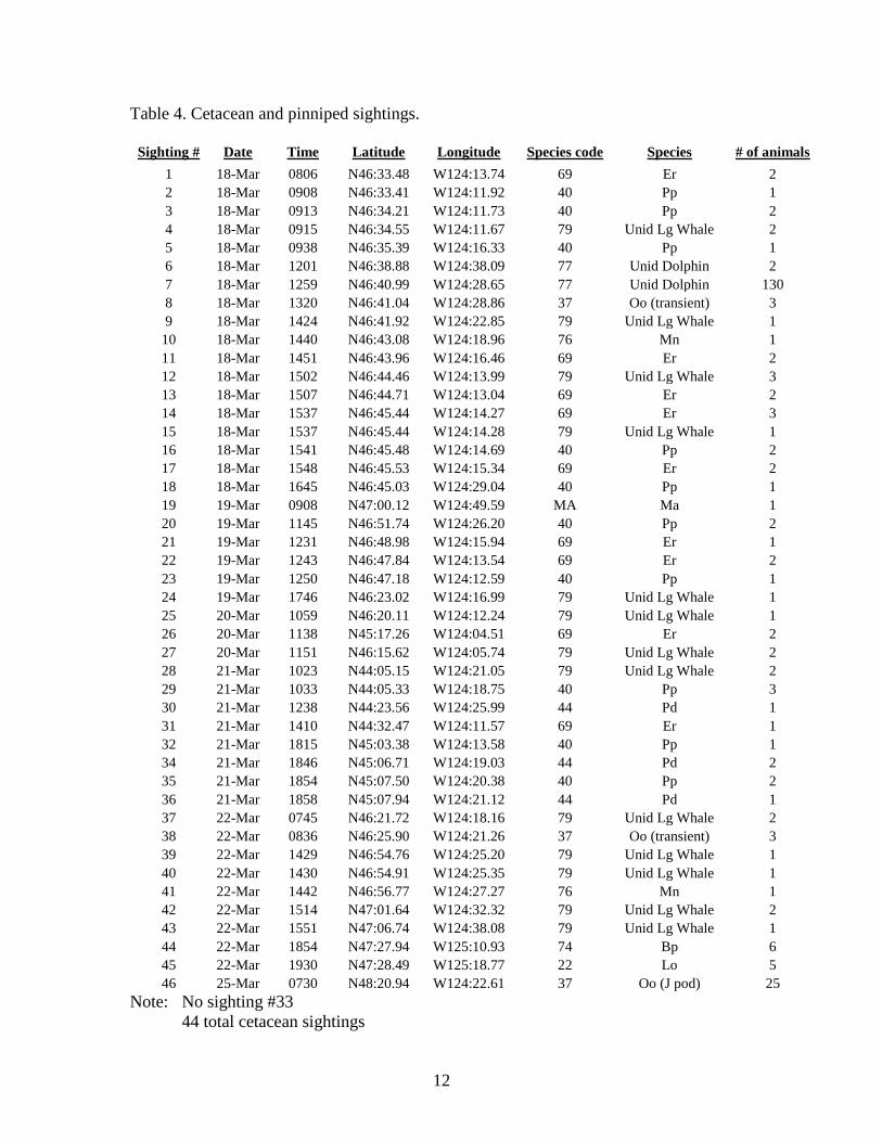
Table 4. Cetacean and pinniped sightings.

Sighting # Date Time Latitude Longitude Species code Species # of animals

1 18-Mar 0806 N46:33.48 W124:13.74 69 Er 2

2 18-Mar 0908 N46:33.41 W124:11.92 40 Pp 1

3 18-Mar 0913 N46:34.21 W124:11.73 40 Pp 2

4 18-Mar 0915 N46:34.55 W124:11.67 79 Unid Lg Whale 2

5 18-Mar 0938 N46:35.39 W124:16.33 40 Pp 1

6 18-Mar 1201 N46:38.88 W124:38.09 77 Unid Dolphin 2

7 18-Mar 1259 N46:40.99 W124:28.65 77 Unid Dolphin 130

8 18-Mar 1320 N46:41.04 W124:28.86 37 Oo (transient) 3


10 18-Mar 1440 N46:43.08 W124:18.96 76 Mn 1

11 18-Mar 1451 N46:43.96 W124:16.46 69 Er 2


13 18-Mar 1507 N46:44.71 W124:13.04 69 Er 2

14 18-Mar 1537 N46:45.44 W124:14.27 69 Er 3


16 18-Mar 1541 N46:45.48 W124:14.69 40 Pp 2

17 18-Mar 1548 N46:45.53 W124:15.34 69 Er 2

18 18-Mar 1645 N46:45.03 W124:29.04 40 Pp 1

19 19-Mar 0908 N47:00.12 W124:49.59 MA Ma 1

20 19-Mar 1145 N46:51.74 W124:26.20 40 Pp 2

21 19-Mar 1231 N46:48.98 W124:15.94 69 Er 1

22 19-Mar 1243 N46:47.84 W124:13.54 69 Er 2

23 19-Mar 1250 N46:47.18 W124:12.59 40 Pp 1



26 20-Mar 1138 N45:17.26 W124:04.51 69 Er 2



29 21-Mar 1033 N44:05.33 W124:18.75 40 Pp 3

30 21-Mar 1238 N44:23.56 W124:25.99 44 Pd 1

31 21-Mar 1410 N44:32.47 W124:11.57 69 Er 1

32 21-Mar 1815 N45:03.38 W124:13.58 40 Pp 1

34 21-Mar 1846 N45:06.71 W124:19.03 44 Pd 2

35 21-Mar 1854 N45:07.50 W124:20.38 40 Pp 2

36 21-Mar 1858 N45:07.94 W124:21.12 44 Pd 1


38 22-Mar 0836 N46:25.90 W124:21.26 37 Oo (transient) 3



41 22-Mar 1442 N46:56.77 W124:27.27 76 Mn 1



44 22-Mar 1854 N47:27.94 W125:10.93 74 Bp 6

45 22-Mar 1930 N47:28.49 W125:18.77 22 Lo 5

46 25-Mar 0730 N48:20.94 W124:22.61 37 Oo (J pod) 25

Note: No sighting #33

44 total cetacean sightings

13

Table 5. Marine bird survey effort, in linear distance surveyed by day.

Survey Date Total kilometers surveyed

18 March 2008 132.53

19 March 2008 138.53

20 March 2008 96.5

21 March 2008 174.63

22 March 2008 147.97

23 March 2008 121.02

24 March 2008 120.63

Total 931.68

14

Table 6. Seabird species observed during marine bird survey effort. Species are listed in

descending order of numerical importance; counts include both flying birds and birds on

the water.

Common name Scientific name Total

count

Percentage

of total

Common murre Uria aalge 3564 59.28

Black-legged kittiwake Rissa tridactyla 829 13.79

Rhinoceros auklet Cerorhinca monocerata 440 7.32

Cassin's auklet Ptychoramphus aleuticus 241 4.01

Western x glaucous-winged

gull

Larus occidentalis x glaucescens 183 3.04

Northern fulmar Fulmarus glacialis 153 2.54

Unidentified dark shearwater Puffinus spp. 73 1.21

Short-tailed shearwater Puffinus tenuirostris 64 1.06

Mew gull Larus canus 56 0.93

Surf scoter Melanitta perspicillata 48 0.80

Red-breasted merganser Mergus serrator 47 0.78

Unidentified gull Larus spp. 46 0.77

Herring gull Larus argentatus 37 0.62

Brant Branta bernicla 34 0.57

Western gull Larus occidentalis 32 0.53

Pigeon guillemot Cepphus columba 22 0.37

Black-footed albatross Phoebastria nigripes 20 0.33

Glaucous-winged gull Larus glaucescens 20 0.33

Brandt's cormorant Phalacrocorax penicillatus 17 0.28

Unidentified alcid Family Alcidae 16 0.27

Sooty shearwater Puffinus griseus 14 0.23

Ancient murrelet Synthliboramphus antiquus 13 0.22

Red-throated loon Gavia stellata 9 0.15

California gull Larus californicus 6 0.10

Double-crested cormorant Phalacrocorax auritus 3 0.05

Western grebe Aechmophorus occidentalis 3 0.05

Harlequin duck Histrionicus histrionicus 2 0.03

Manx shearwater Puffinus puffinus 2 0.03

Marbled murrelet Brachyramphus marmoratus 2 0.03

Pacific loon Gavia pacifica 2 0.03

Thayer's gull Larus thayeri 2 0.03

Unidentified murrelet Family Alcidae 2 0.03

Canada goose Branta canadensis 1 0.02

Common loon Gavia immer 1 0.02

Fork-tailed storm-petrel Oceanodroma furcata 1 0.02

15

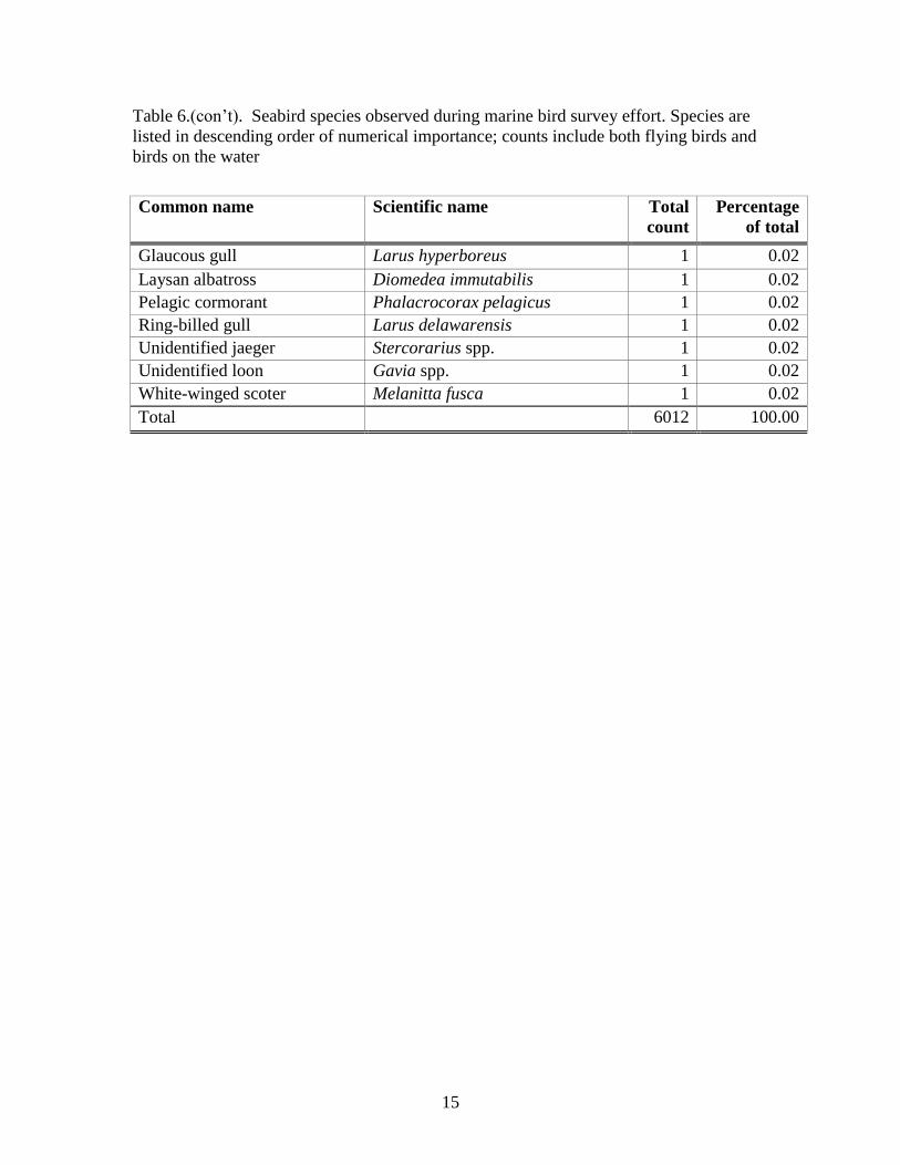
Table 6.(con’t). Seabird species observed during marine bird survey effort. Species are

listed in descending order of numerical importance; counts include both flying birds and

birds on the water

Common name Scientific name Total

count

Percentage

of total

Glaucous gull Larus hyperboreus 1 0.02

Laysan albatross Diomedea immutabilis 1 0.02

Pelagic cormorant Phalacrocorax pelagicus 1 0.02

Ring-billed gull Larus delawarensis 1 0.02

Unidentified jaeger Stercorarius spp. 1 0.02

Unidentified loon Gavia spp. 1 0.02

White-winged scoter Melanitta fusca 1 0.02

Total 6012 100.00

16

Table 7. Acoustic detections of marine mammals

Date Time Latitude Longitude 1st detection Species Ecotype

3/17/2008 20:50 46.2044 -124.6274 Acoustics

O.o. or

P.m.? N/A

3/18/2008 08:19 46.5735 -124.1910

Acoustics on

Flying Bridge O. orca Unknown

3/18/2008 13:22 46.6854 -124.4726 Visual O. orca Transient?

3/19/2008 16:11 46.4882 -124.5916

Acoustics on

Flying Bridge O. orca

Offshore or

Resident?

03/22/08 06:17 46.2228 -124.476 Acoustics

O.o. or

P.m.? N/A

3/22/2008 8:45 46.4474 -124.3539 Visual O. orca

Possible

Transient

3/25/2008 4:00 48.4731 -124.6445 Acoustics O. orca S.R. J-Pod

Table 8. Killer whale encounters.

Date Duration of

encounter

Latitude Longitude Ecotype Whales Present

3/18/2008 ~ 40 minutes 46.6854 -124.4726 Transients Unk.

3/22/2008 2hr 18min 46.4474 -124.3539 Transients Unk.

3/25/2008 9hrs 27min 48.4731 -124.6445 Resident J pod

Table 9. Summary of environmental data.

Sample type Cruise total

CTD casts 6

CTD chlorophyll samples 57

Surface chlorophyll samples 47

Nutrient samples 60

Salinity samples 22

XBT drops 25

17

Table 10. XBT deployment locations

XBT # Serial # Max depth

(m)

Sea surface

temp (°C)

PST

Date

PST

time

Latitude (N) Longitude (W)

1 973138 68 8.5 3/18/08 956 46 35.64 124 19.93

2 973134 163 8.5 3/18/08 1200 46 38.49 124 39.82

3 973130 370 8.7 3/18/08 1819 46 46.68 124 51.92

4 973129 160 8.4 3/19/08 900 47 00.27 124 48.39

5 973133 65 8.7 3/19/08 1200 46 50.95 124 23.02

6 973137 156 8.5 3/19/08 1500 46 36.94 124 36.50

7 1006009 174 8.8 3/20/08 900 45 31.18 124 20.60

8 1006013 96 9.0 3/20/08 1200 45 15.07 124 07.13

9 1006017 175 9.0 3/20/08 1500 45 00.17 124 19.63

10 1006014 99 9.0 3/20/08 1945 44 40.30 124 25.00

11 1006018 124 9.0 3/21/08 900 44 03.70 124 40.59

12 1006010 84 9.1 3/21/08 1200 44 17.95 124 23.08

13 1006019 72 9.4 3/21/08 1500 44 39.42 124 15.64

14 1006015 73 8.0 3/22/08 1000 46 25.22 124 19.39

15 1006011 132 8.4 3/22/08 1200 46 32.70 124 28.12

16 1006012 71 8.6 3/22/08 1500 46 59.21 124 29.75

17 1006016 149 7.8 3/23/08 900 48 12.43 123 41.94

18 1006020 161 7.9 3/23/08 1200 48 22.52 124 07.65

19 1005916 134 8.1 3/23/08 1500 48 23.45 124 30.71

20 1005920 243 8.2 3/24/08 900 48 28.75 124 37.91

21 1005924 140 8.2 3/24/08 1200 48 14.21 124 00.84

22 1005915 156 7.8 3/24/08 1522 48 21.24 124 03.27

23 1005919 181 8.1 3/25/08 920 48 21.63 124 25.39

24 1005923 169 8.0 3/25/08 1200 48 30.91 124 34.20

25 1005914 54 8.2 3/25/08 1500 48 39.11 124 57.33

Table 11. CTD deployment locations.

CTD #

Number of

depths sampled

Max depth

(m)

Local

Date PST

Local Start

Time PST

Lat (decimal

degrees)

Long (decimal

degrees)

1 12 1010 3/17/08 2031 46.79 -125.29

2 12 700 3/18/08 2036 46.24 -124.57

3 11 425 3/20/08 2030 45.26 -124.60

4 12 1000 3/21/08 2035 47.56 -125.45

5 9 130 3/22/08 2038 48.36 -124.06

6 10 175 3/23/08 2037 48.29 -124.16

18

Figure 1. Cruise track of the McArthur II from 17 - 26 March 2008.

19

Figure 2. Visual On and Off – effort monitoring of marine mammals from 17 - 26 March 2008.

20

Figure 3. On and Off- effort sightings of marine mammals from 17 - 26 March 2008.

21

Figure 4. Acoustic detections of marine mammals from 17 - 26 March 2008.

22

Figure 5. XBT and CTD deployments from 17 - 26 March 2008.