


Languages
Pages
Legal


IN DEGREE PROJECT COMPUTER SCIENCE AND ENGINEERING,SECOND CYCLE, 30 CREDITS
, STOCKHOLM SWEDEN 2019
Optimizing LTE test traffic using search- and expert algorithms
WILLIAM SCHRÖDER
KTH ROYAL INSTITUTE OF TECHNOLOGYSCHOOL OF ELECTRICAL ENGINEERING AND COMPUTER SCIENCE


Optimizing LTE test traffic using search- and expert algorithms
William Schröder
Master thesis in computer science (30 credits) at the school of computer science and engineering
Royal Institute of Technology 2019-05-26
Supervisor at CSC was Anders Holst Examiner was Örjan Ekeberg

Abstract This thesis investigates whether artificial intelligence techniques can replace
the optimization process that is currently performed by experts for LTE/4G
stability tests at Ericsson. The investigation covers the usage of search
algorithms and expert systems and the thesis then implements a hybrid
algorithm. This implemented solution is then tested upon three different
architectures to judge how well it optimizes tests without causing further
problems. The conclusion is that the implemented solution optimizes tests
sufficiently but does so using only mobile users. To reflect reality better, static
users would also need to be included in the optimization process.

Sammanfattning Syftet med det här exjobbet är att undersöka huruvida tekniker baserade på
artificiell intelligens skulle kunna ersätta de optimeringssteg som för
närvarande görs av experter under stabilitetstester för LTE/4G vid Ericsson.
Bakgrundsundersökningen täcker sökalgoritmer och expertsystem och en
hybridalgoritm har sedan implementerats. Ett experiment har därefter
genomförts på tre olika testfall för att utvärdera den implementerade
algoritmens förmåga att optimera test utan att introducera nya problem i
testet. Slutsatsen är att optimeringen har tillräcklig effekt men att detta endast
görs genom att omfördela mobila användare. Statiska användare skulle också
behöva inkluderas i algoritmen för att göra dess optimeringar mer realistiska.

Table of Contents 1 Introduction............................................................................................................................. 1
1.1 Problem description ..................................................................................................... 1
1.2 Objective ............................................................................................................................ 2
1.3 Scope ................................................................................................................................... 2
1.4 Evaluation ......................................................................................................................... 2
1.5 Outline ................................................................................................................................ 3
1.6 Terminology ..................................................................................................................... 3
2 Background .............................................................................................................................. 5
2.1 LTE technology ............................................................................................................... 5
2.2 Lab environment ............................................................................................................ 6
2.2.1 Architecture.............................................................................................................. 7
2.2.2 UE assignment ......................................................................................................... 8
2.2.3 Test execution and evaluation .......................................................................... 8
2.2.4 Optimal test configuration .............................................................................. 11
3 Related methods ................................................................................................................. 13
3.1 Optimization problems ............................................................................................ 13
3.2 Local search algorithms ........................................................................................... 14
3.2.1 Heat based search ............................................................................................... 16
3.2.2 Multi-start search................................................................................................ 17
3.2.3 Genetic algorithm ................................................................................................ 19
3.2.4 Multi-neighbor search....................................................................................... 20
3.2.5 Alternating neighborhood search ................................................................ 21
3.3 Knowledge based systems ...................................................................................... 21
3.3.1 Rule based .............................................................................................................. 22
3.3.2 Fuzzy logic .............................................................................................................. 22
3.3.3 Training based...................................................................................................... 24
3.3.4 Analysis ................................................................................................................... 24

3.4 Hybrid algorithms ...................................................................................................... 24
3.4.1 Interpolation with expert system ................................................................ 25
3.4.2 Optimizing binary search with expert system........................................ 25
3.5 Flow networks ............................................................................................................. 25
4 Method .................................................................................................................................... 27
4.1 Problem formalization ............................................................................................. 27
4.2 Node traffic discovery ............................................................................................... 28
4.3 Cell traffic optimization ........................................................................................... 28
4.4 Solution strategy ......................................................................................................... 29
4.5 Node level formula analysis ................................................................................... 30
4.6 Cell level formula analysis ...................................................................................... 31
4.7 Node level traffic redistribution ........................................................................... 31
4.8 Cell level traffic redistribution .............................................................................. 32
4.8.1 The flow network approach ........................................................................... 32
4.8.2 Multiple bad cells ................................................................................................ 35
4.8.3 Handover types priority ................................................................................... 36
4.8.4 Net flow between nodes ................................................................................... 36
5 Experiment............................................................................................................................ 37
5.1 Node level formula analysis ................................................................................... 37
5.2 Cell level formula analysis ...................................................................................... 37
5.3 LTE test configuration .............................................................................................. 38
5.3.1 Formulae used ...................................................................................................... 39
5.3.2 Test cases................................................................................................................ 39
5.4 Evaluation metrics ..................................................................................................... 41
5.5 Results ............................................................................................................................. 41
6 Discussion.............................................................................................................................. 44
6.1 Analysis ........................................................................................................................... 44
6.2 Criticism.......................................................................................................................... 45

6.3 Alternative solutions ................................................................................................. 45
7 Conclusion ............................................................................................................................. 47
8 References ............................................................................................................................. 48

1 - Introduction
1
1 Introduction The theme of this thesis is search algorithms and expert systems. The purpose
is to investigate whether algorithms in these fields can be deployed in time
constrained environments with no previous knowledge and still perform with
adequate results.
1.1 Problem description The problem of this thesis is provided by the LTE stability team of Ericsson.
Their objective is to ensure that the specifications of the radio base stations
sold by Ericsson to its customers pass the stability requirements. To
accomplish this, they regularly perform tests in their networks with simulated
roaming users. The requirements tested form a subset of the many test
demands that exists across Ericsson and are for the stability team focused on
analyzing how the base stations react to multiple users switching to and from
its coverage zones. For each test, they specify the hardware of the base
stations being tested as well as the initial number of users throughout the
network. The goal is to have as many handovers between the base stations as
possible without them showing any indications of instability in the test
results.
Because tests take considerable time to run (around 3 hours), the
configuration steps are very delicate. As the team configure the tests to be on
the borderline of what the base stations can handle, there is an overwhelming
risk of there being too much, causing instability. In these cases, the testers
must analyze the test results and try to come up with a new configuration that
would remove the errors, while reducing the number of handovers as little as
possible. This process is far from trivial and takes up a lot of the testers’ time.
Thus, there is a need to have an artificial intelligence help the testers
determine how to redistribute the simulated users in order for the next test to
pass the requirements. Ideally, the algorithm should be able to run
autonomously overnight, allowing the system multiple iterations of
improvements to reach the optimal configuration.
The considerable amount of time it takes to run a test is also the source of the
uniqueness of this problem, which is that data points required for the
optimization are expensive to produce. Thus, the contributions of this thesis

1 - Introduction
2
are: a literature study on optimization methods with this constraint in mind; a
theoretical suggestion of how an iterative algorithm for solving the described
problem can be designed; and an implementation and evaluation of the
algorithm for a single step in this iteration. Simulated tests, like the ones used
in this thesis, contributes to a sustainable environment by avoiding the need
for some hardware tests, reducing power consumption. By automating these
tests, this thesis also makes a contribution in sustainability. Ethical concerns
are not an issue as the work is done in automation which affects nothing but the tests ran of one tester on simulated equipment.
1.2 Objective The goal of the thesis is to investigate what algorithms can be used to solve
the test optimization problem and to do a comparison between these. The
primary objective is to find an algorithm which reliably suggest improvements
to a test configuration given its latest results. This algorithm must provide
improvement suggestions that accommodate all the experts’ requirements
while minimizing the reduction of handovers. There can be no requirement on
training data as no test history is being kept of how different configurations
yield what results. A secondary objective has also been set out. The suggested
algorithm should be able to run multiple iterations and use results from more
than one set of test results during optimization.
The specific problem statement is
Can an algorithm that suggests optimizations to LTE mobility tests be
constructed? If so, could such algorithm be designed to converge using
test results of multiple iterations?
1.3 Scope Only one iteration of the proposed algorithm is tested in the test networks.
Also, out of the discussed theoretical alternatives only one implementation
could be tested for availability reasons.
1.4 Evaluation From Ericsson’s perspective, evaluating the effectiveness of the
implementation concerns measuring the usefulness of the test configuration
suggestions it provides to the testers. Ideally, these would be evaluated by

1 - Introduction
3
comparing the results of a test conducted with the initial configuration with
one using the configuration suggested by the proposed algorithm. However,
for practical purposes this was not possible and thus the evaluation will
instead be based on a function provided by the experts. This leads to the
following evaluation formulation:
The algorithm is given an initial test configuration and the
corresponding test results to find a better configuration. The suggested
changes are then analyzed using a function formulated by the experts to
deduce how likely they are to lead to improved test results. If the
evaluation suggests the changes should yield improved results, the
algorithm has been successful.
To ensure the algorithm can handle a variety of test scenarios, the algorithm is
tested upon three typical test configurations. These are:
1. A small test (few routes), testing the algorithm’s operating capacity
when the setting is constrained.
2. A medium sized test (standard routes), aimed to symbolize the
general usage case.
3. A large test (many routes), challenging the algorithm to make
optimal assignments when the solution space is larger.
1.5 Outline The thesis first covers the details of LTE as a background to understanding the
tests conducted. This knowledge is then used to model the underlying
optimization problem and to divide it into sub-problems. Each such sub-
problem is then investigated individually with a literature study to determine
which algorithms to pursue in the implementation phase. Next, parts of the
algorithm are implemented and evaluated using the previously described
strategy.
1.6 Terminology This section is meant as a quick summary of the terms used in this report.
Each of the terms is more thoroughly described later in the report.
LTE: The technical term for 4G technology.

1 - Introduction
4
Node: Also referred to as ENB this is the abbreviation for radio base
stations used in 4G/LTE and is represented as n.
Cell: A subcomponent of a node which provides coverage in a certain
direction. It can be visualized as a circular arc originating from the node
where users can connect to the node. Cells are represented as c. A cell c
is considered to belong to a node n if c is a subcomponent of n.
Route: A path describing user movement between two cells, thus
performing a specific handover between these cells. Routes have a
handover type and are represented as r. A route r is considered to
belong to a cell c if r has an endpoint in c. Similarly, r is considered to
belong to a node n if there is a cell c such that r belongs to c and c
belongs to n.
Handover type: A protocol the cells use when performing a handover
of users to another cell. Can be either S1, X2, intra or irat.
Traffic: Also referred to as load or less accurately as UEs or users;
traffic is an intensity measurement of how many handovers that are
performed during a given time period. Traffic is represented as t and is
a property of routes, in which case tr represents the amount of traffic on
route r.
Formula: A specific test result field, presented in success- or failure
rate. An example would be node level handover rejects due to high load.
Formulae are represented as f. Formula measurement denotes the
value a specific formula has for a given test. Formula filter is the
function which returns a Boolean value as to whether a formula
measurement is within the tolerance range or not.

2 - Background
5
2 Background As a prerequisite to analyzing the optimization problem that is the basis for
the implementation, this section covers the basics of LTE technology as well as
a more detailed description of the test networks in the stability team.
2.1 LTE technology The test network that is being utilized in this thesis is a simulation of the LTE
network, sometimes referred to as 4G. At the time of writing (March 2017)
this is the most recent cellular communication technology. It consists of these
components:
• The User Equipment (UE).
• The Evolved UMTS Terrestrial Radio Access Network (E-UTRAN).
• The Evolved Packet Core (EPC).
See figure 2-1 below for a diagram of the subsystems.
Figure 2-1: LTE network architecture
The UEs corresponds to user held devices, such as cell phones or tablets, that
are connected to the LTE network. They each contain a sim card which
identifies them across the network. There are various categories and
properties of the UEs but for this thesis they can simply be considered as
users.
The E-UTRAN is the subsystem in closest proximity to the UEs and provide the
access points to the LTE infrastructure, known as eNodeBs (ENB), henceforth
abbreviated as nodes. These are the LTE correspondents to what in GSM is
known as the Radio Base Stations (RBS) and act as links between the UEs and
the packet core (EPC). The nodes are also responsible for controlling the
operations of its connected UEs which among other things includes handling
handovers to other nodes when the UEs leave its area of operations. To
accomplish these objectives, two communication interfaces are available to

2 - Background
6
the nodes, (Poole, n.d.). The S1 interface is used to communicate with the EPC.
The main form of data transferred through this interface is user data
transmitted between nodes and the EPC, i.e. network data. The other available
interface, X2, is more commonly used to communicate handover information
with other nodes directly as the UEs leave one node for another. See figure 2-2
for an overview of the E-UTRAN subsystem.
Figure 2-2: LTE access network
Additionally, there is a third interface, known as irat, used for communicating
handover information to nodes of other mobile technologies should UEs move
from an LTE node to, say a WCDMA NB (the 3G correspondent of a node).
There are also instances where handovers within the LTE network would run
over the S1 interface rather than through X2, which is normally employed.
This means that the handovers are communicated through the EPC layer
rather than through direct communication between two nodes.
2.2 Lab environment This section focuses on the test network environment at 4G Stability. There
are a variety of configuration settings for these networks, the ones of interest
to this thesis are:
• The test network architecture which describes the hardware and the
handover types of the UEs.
• The amount of traffic on each component of the architecture.
The rest of this chapter covers these configurations in order as well as a
description of how tests are executed and evaluated.
2 - Background
7
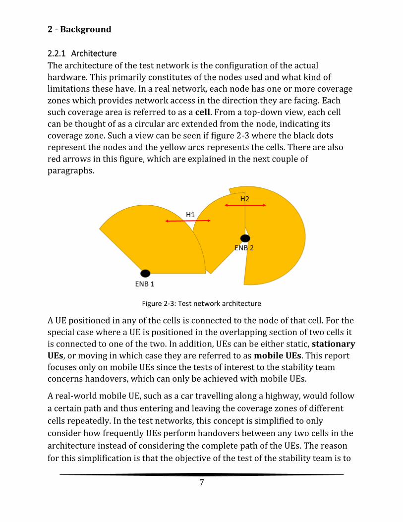
2.2.1 Architecture
The architecture of the test network is the configuration of the actual
hardware. This primarily constitutes of the nodes used and what kind of
limitations these have. In a real network, each node has one or more coverage
zones which provides network access in the direction they are facing. Each
such coverage area is referred to as a cell. From a top-down view, each cell
can be thought of as a circular arc extended from the node, indicating its
coverage zone. Such a view can be seen if figure 2-3 where the black dots
represent the nodes and the yellow arcs represents the cells. There are also
red arrows in this figure, which are explained in the next couple of
paragraphs.
Figure 2-3: Test network architecture
A UE positioned in any of the cells is connected to the node of that cell. For the
special case where a UE is positioned in the overlapping section of two cells it
is connected to one of the two. In addition, UEs can be either static, stationary
UEs, or moving in which case they are referred to as mobile UEs. This report
focuses only on mobile UEs since the tests of interest to the stability team
concerns handovers, which can only be achieved with mobile UEs.
A real-world mobile UE, such as a car travelling along a highway, would follow
a certain path and thus entering and leaving the coverage zones of different
cells repeatedly. In the test networks, this concept is simplified to only
consider how frequently UEs perform handovers between any two cells in the
architecture instead of considering the complete path of the UEs. The reason
for this simplification is that the objective of the test of the stability team is to

2 - Background
8
provide specifications of the node capabilities individually, rather than
analyzing mobile UEs’ impact on the complete architecture. For this reason,
test UEs are defined using routes which represent a specific handover
between two cells of the same or different nodes. figure 2-3 depicts routes as
red arrows between two cells, indicating all mobile UEs on this route would
perform a handover between these two cells. In the same figure, there are two
routes, defined as H1 and H2. These routes have a significant difference as H1
is an inter-route between different nodes while H2 is an intra-route between
two cells of the same node. Recall from the
LTE technology section that inter-routes can be conducted using three
different protocols, S1 (via the EPC interface) and X2 (direct node to node
handover) or irat (to a node of another mobile technology). Handovers using
intra-routes do not have any associated handover type.
2.2.2 UE assignment
With the infrastructure fully configured using the architecture, the next step is
to put traffic into the test. Traffic is represented by a set amount of mobile
UEs that operate on a certain route, thus performing the handover stated by
this route. Thus, by increasing traffic on a route, the connected nodes will
have a higher load since they need to deal with more handovers. Ideally, the
load on each node in the test should be as close as possible to the hardware
limitations without exceeding them.
2.2.3 Test execution and evaluation
After a test has been configured with architecture and traffic, it is executed in
one of the test networks. During the test run, traffic is simulated with various
intensity between low and high peaks. The evaluation measurements for the
test is accessible as soon as the test starts, but at this stage everything is zero.
The longer the test runs the more accurate these measurements are. Tests are
always deterministic meaning two tests that run with the same configuration
produces the same results.

2 - Background
9
Evaluating the results of a test is done by examining the results of
measurements known as formulae1. The full evaluation results of a test
involve hundreds of different formulae, each describing how well the test
went with respect to some parameters, whereof only a handful are relevant to
the stability team. Formulae are separated into two categories: node- and cell
level. An example would be ‘handovers rejects due to high load’ which is a
node-level formula depicting the number of attempted handovers that failed
due to the node already operating at peak capacity. A formula can also be
defined on the cell level, then referred to as cell-level formula. All future
references to formulae refer to the subset of formulae that are relevant for the
stability team.
The value of each formula, referred to as formula measurement is presented
in percent. Node-level formulae indicate rates of failure, meaning the goal is to
be as low as possible, while cell-level formulae indicate rates of success and
should thus be maximized. Furthermore, the formulae have a tolerance range
where architecture components performed adequately. The Boolean value for
a specific formula is referred to as formula filter and is denoted by g where
g(f) is True if the formulae measurement of f is within the tolerance range of f.
Since the formulae of interest varies from test to test, including the tolerance
ranges, these parameters must be specified as input to each test.
As the traffic intensities vary throughout the test, so does the evaluation
measurements. For this reason, formulae measurements are sampled at
specific time intervals of 15 minutes or more. Figure 2-4 depicts such an
interval sampling during the time period 08:15 to 17:15 using a sampling
interval of 60 minutes. Two test runs are visible in the graph, one which was
started before 08.15 and ended around the graph dip at 11.15. Another test
was then started which finished around 17.15.
1 The name formula originates from the fact that evaluation measurements are based on some sort of calculation (i.e. successful attempts divided by total attempts) and thus it is said that the evaluation measurements is the result of a formula.

2 - Background
10
Figure 2-4: Formulae measurement sampling
Experts of the stability team have analyzed the relationship between load and
formulae measurements and determined that the behavior of this function is
too complex in nature to be used for optimization in the general test case.
Thus, the formulae measurements of each test must be analyzed separately.
The experts have also provided some general information as to how load
relates to formulae measurements. For the node level, formulae
measurements are expected to have a roughly linear relationship with traffic.
On the cell level however, reducing load on a cell marginally affects the
formulae measurements of that cell until a certain point where there is a rapid
improvement in formulae measurements. A schematic illustration is depicted
in Figure 2-5.

2 - Background
11
Figure 2-5: Schematic illustration of formulae measurements relationship with load.
2.2.4 Optimal test configuration
With the details of the test environment covered, the question is now how the
thesis’ goal should be reached, i.e. how to construct the optimal test. There are
two factors contributing to evaluating the quality of the tests:
• The formulae filters, indicating to what extent the hardware passed the
set-up requirements. The more formulae passed, the better the results.
• The amount of traffic, indicating how much pressure the hardware was
under. The more traffic, the more useful the results.
Between these factors, it is more important to pass the configured formulae
filters than having much load on the node. Thus, the goal when optimizing the
test can be expressed as “configuring the test with maximum possible traffic
amount on each node such that the test still passes the formulae filters”.
Should one or more nodes or cells not pass any of the corresponding formulae
filters then those are considered bad nodes or bad cells. In such cases, the
bad nodes and/or cells needs to have their traffic reduced. The most straight
forward way of performing this traffic reduction would be to remove static
UEs from the bad node/cell. However, since the stability team is interested in
Form
ula
mea
surm
ent
Load
Schematic illustration of the load-formula measurement
relationship
Cell level Node level

2 - Background
12
testing how the nodes’ capacity in handling handovers, the traffic reduction
has to be made with mobile UEs. Recall from the Architecture section that
mobile UEs are added using routes between different cells, and thus that there
is a conflict of interest between the connected cells as to what the reduction
should be.
Thus, configuring an optimal test is a matter of finding traffic assignments
to routes in such a way that all formulae filters for each node and cell in
the architecture pass while traffic is maximized on each node. This is the
formulation for the underlying optimization problem which is analyzed
further in the Method section.

3 - Related methods
13
3 Related methods This section covers the basis of the algorithms designed later in the report. Its
primary function is to act as a resource for the reader to further understand
these underlying concepts before proceeding with the report. The main points
of this chapter are basics on optimization problems, local search algorithms,
knowledge based systems and flow networks.
3.1 Optimization problems Optimization problems can be defined as the following: “for a given problem
with a space of solutions, find the best such solution”. The solution space
consists of a set of unknown variables where a valid assignment of these
variables is a potential solution to the problem. To determine the best
solution, an objective function that depends on these variables is used. The
goal when solving the optimization problem is to either minimize or maximize
the objective function by configuring the variables.
Moreover, the range of the variables in the solution space determines the
characterization of the optimization problem. Firstly, the solution space can
be discrete or continuous and can also be subject to constraints in what is
then defined as a constrained optimization problem. Constraints can either
be defined as a relationship- or range limitations of the variables in the
solution space. Additionally, the optimization problem can have either zero,
one or multiple objectives. While one objective function is common, multiple
objective functions are also possible (e.g. finding the cheapest and quickest
flight available). In these cases, one normally must specify a weight for the
different objectives (e.g. finding a cheap flight that should also be quick if
possible) for the objective requirement(s) to be interpreted correctly. The
case of zero objectives is also interesting, in this case the goal is simply to find
a legal variable assignment. An evaluation function is used to evaluate how
well a solution matches the objectives.
When faced with an optimization problem, there are two different approaches
to finding a solution. The most obvious one, a solver, solves an instance of the
problem. The other approach, a modeler, attempts to find relationships
between constraints and variables to analyze the problem in the general case.

3 - Related methods
14
To illustrate the difference between these methods, consider the problem of
finding the quickest flight path between London and New York. The solution
of this problem varies from day to day due to the air corridor allocation,
weather etc. These factors limit the options and thus they are constraints in
this constrained optimization problem. To find a solution for a certain time
where the air corridors and weather conditions are given, a solver would be
employed to find the solution. If, however, the goal is to analyze the general
form of the problem (i.e. without knowing the air corridors and weather
conditions) then a modeler would be used to identify relationships between
the constraints and the solution.
3.2 Local search algorithms A local search algorithm is a method used to solve optimization problems. In
addition, it is often used to improve existing solutions that other algorithms
have found. A good example of this is the TSP problem. Assume that another
algorithm has already found a solution to a certain instance and the question
is now if it is possible to start from the solution and try to find improvements.
A local search algorithm can accomplish this by exploring two of the paths
found in the previous algorithm and investigate whether the route would be
faster by switching these two routes. This process is referred to as 2-opt and
is quick to run since one iteration of the algorithm takes constant time. This
optimization has proven to outperform even the best algorithms designed to
solve the TSP problem (Johnson & McGeoch, 1995). The search can also take
the name n-opt if more than two paths are considered at once.
The general solving process of a local search algorithm involves improving an
existing solution step by step by exploring neighboring solutions and adopt
those that appear promising, with the hopes of ending up at the goal. As a
metaphor, imagine that you are in the middle of a maze and must find a way
out. You see four different paths available, and while none of the paths
immediately leads to the goal, the visible length of path A is longer than any of
the other paths. Judging by this information, path A seems the most promising
since it allows for the most movement. The view of a local search algorithm
very much resembles this example. It explores neighboring solutions and
applies changes on a local level to traverse the search space. Just as a human
exploring a maze, its terminating conditions are either reaching the goal

3 - Related methods
15
(getting out of the maze) or exceeding the time limit (giving up) stating how
close to the goal it came.
Local search algorithms face an important challenge with local optima. To
understand this dilemma, consider a simple search algorithm known as hill
climbing. In this algorithm, a blind, one-dimensional man traverses a x*sin(x)
graph starting from x=0 with the hopes of reaching the highest peak, starting
at x=0. He will reach the first peak at x=2 thinking he has reached the highest
point, while in fact there are other mountains in the distance which would in
fact be higher peaks than where he is currently at. In more mathematical
terms, the peak found by the blind man is a local maximum but not the global
maximum he was seeking. This problem of getting stuck a local maximum is
one a local search algorithm is often faced with and there are various
improvements that can be conducted to avoid this issue.
To address the problem of local optima as well as speeding up the search, the
paper “A local search template” (Vaessens, Aarts, & Lenstra, 1997) starts from
the basic local search version and tries to come up with improvements. The
basic local search template considered by the author is the deterministic
iterative improvement algorithm which is another name for the previously
described example of local search when finding the way out of a maze. As a
recap, consider a local search algorithm that explores all its immediate
neighbors before picking the most promising one. The algorithm then accepts
this best neighbor as its current states and continues the search from there
until no further improvements can be made. The authors suggest various
categories of improvements to this algorithm:
• Exploring many neighbors at once, resulting in a multi-neighbor
search. This is the opposite of the single-neighbor search which is
referred to as the best improvement algorithm.
• Starting the search from various starting points, referred to as a multi-
start search.
• Allowing the neighbor function to accept worse states on certain
occasions to avoid getting stuck in local optima, called heat based
algorithms.
• Replacing the concept of current solution with a population. This
approach takes the name of a genetic algorithm.

3 - Related methods
16
• Alternating between different neighborhood functions to try to get the
best of multiple worlds. This is referred to as alternating
neighborhood search.
The remainder of this section covers each of these proposed improvements in
turn and analyze how they can be used to model the local search for the
formula analysis. Throughout these subsections, it is important to keep in
mind that algorithm running time is not an issue, since this time is negligible
compared to the time it takes to perform a test (at least an hour). Instead, a
desirable property of the formula analysis is to perform the local search while
doing as few “reads” as possible. The reason being that a test of three hours
needs to run for every such read and thus the time available for the algorithm
decreases very quickly as multiple reads are being conducted.
3.2.1 Heat based search
This category considers two algorithms, simulated annealing and tabu search.
Simulated annealing is an algorithm that involves using a random variable
which allows the local search to sometimes accept moving to a worse
neighbor compared to the current state. The goal of this is strategy is for it to
avoid getting stuck in local maxima and continue the search for the global
maximum, initially by moving to a worse solution. Its name comes from the
annealing process in the metal industry, which is used when shaping metal
objects. Initially, the material must be very hot for the worker to be able to
shape it and as the material cools, it becomes increasingly robust. The same
strategy is used in the simulated annealing algorithms; initially the
temperature is very high, allowing the algorithms to examine far worse
neighbors but as time progresses, the temperature decreases and the
algorithm has less margin in choosing worse solutions. Finally, after a fixed
amount of runs the temperature is so low that the algorithm is only allowed to
improve by moving to neighboring solutions by which time it has hopefully
found the global optimal value (Jacobson, 2013), (Carr, 2017).
Tabu search has a similar approach to simulated annealing but was originally
intended only as a higher-level heuristic upon which one can implement
another local search algorithm that runs with the help of the tabu search. Just
as simulated annealing, its goal is to allow that local search to surpass local
optima by accepting worse solutions. The difference however, lies in that tabu

3 - Related methods
17
search utilizes a list of previously visited states, tabu lists, which it refers back
to whenever the local search finds a spot where there are no improving
neighbors available. The tabu lists can hence be perceived as an aid for a local
search algorithm to be used whenever there are no improving moves. This
would allow any local search algorithm to be combined with tabu search to
reach the global optimum while avoiding local maxima traps (Gendreau,
2002).
To understand whether this category of solutions improves the local search
for the load reduction discovery, it is important to realize in what scenarios
local maximum are a problem and when they are not. For a monotonic
function, there are no local maxima and thus any maximum value found is also
the global maxima. This might seem obvious, since the maximum value y of a
monotonic increasing function would be the greatest assignment of x.
However, consider the case where the objective is to find the minimum
assignment of x in a monotonic increasing function such that f(x) > c where c
is a constraint given by the problem. Here, the optimal is not the greatest
value of x but the lowest values of x that fulfills the constraints.
As it happens, the function that maps traffic load to formula measurements is
of the monotonic increasing type where the goal is to reduce traffic as little as
possible while still reaching zero on the formula measurements. A discretized
version of this function could then be represented by a sorted array for which
binary search is an efficient solver, with the expectation to conduct log(n)
reads before the optimal solution is reached. For these reasons, the search
algorithm does not need help finding optimal solutions since it does this
already, instead a strategy is sought that could potentially reduce the running
time. Following this line of reasoning, neither simulated annealing nor tabu
search improves performance since both algorithms involves more reads
without improving the solution. The reason being that local optima are not a
problem due to the monotonic nature of the explored function.
3.2.2 Multi-start search
Another interesting improvement option is the multi-start search. There are
at least two different arguments for utilizing this strategy; one is to avoid local
optima and the other is to improve the running time where parallelism is
available. To understand this, consider how multiple starting points decided

3 - Related methods
18
with randomness allows the search to hill climb from various valleys with the
hopes of reaching various mountain tops. This information can then be used
to find the best mountain top which also hopefully is the global optimum. As it
happens multi-search has proven to be more efficient than algorithms such as
simulated annealing in the TSP problem (Boese, Kahng, & Muddu, 1993),
(Johnson, Local Optimization and the Traveling Salesman Problem, 1990).
The next question is to decide how many different starting points to use. The
first intuition is to use as many starting points as the amount of parallelism
available based on the reason that each starting point can then run on its own
thread and thus the exploration of each starting point does not interfere with
the available resources of exploration paths that belong to other origins.
Nevertheless, the multi-start strategy could also be employed in environments
which are single-threaded with the idea of immediately disposing suboptimal
starting points. As an example, consider the optimal load reduction is 17 while
the starting points chosen are 10, 20 and 30. First a test of reduction 10 is
executed, where there would still be indications of bad cells since the
reduction is not low enough. Next, the test of reduction 20 is run, where the
formula shows 0. From this information, it can be deduced that the optimal
load reduction lies between 10 and 20 and thus there is no reason to run
further starting points.
It is also worth mentioning that due to the nature of the formula analysis, the
multi-start search is not applicable. The reason being that the original test
serves as the starting point for the first iteration, hence the algorithm cannot
introduce new starting points. Instead, pseudo-starting points could be
introduced after the first test, i.e. in the second iteration. This would allow the
algorithms to further improve the solution by finding neighbors to these
second iteration starting points.
Nevertheless, it is not clear that this strategy is an improvement to binary
search. Without problem specific information available to the algorithm,
binary search runs quicker due to the monotonic increasing property of the
load/formulae function. Inclusion of problem specific information in the form
of rules is covered in the hybrid algorithms section.

3 - Related methods
19
3.2.3 Genetic algorithm
The most ambitious of all the improvements categories would be to try to
optimize the solver by employing a genetic algorithm. This kind of algorithm,
like its name implies, relies on survival of the fittest when it comes to
exploring neighboring solutions. In a living subject, this process is reflected by
chromosomes where those with the highest fitness tends to be the ones to
survive and reproduce new offspring. When the amount of offspring is zero,
this algorithm does not do a whole lot because it would then progress as
quickly as any other. The advantage comes when considering parallelism. If
the genetic algorithm can consider multiple different solutions (or offspring)
simultaneously, it can use the results to analyze which of these solutions that
are better fit to the problem configuration (Smita Sharma, 2013).
However, for a genetic algorithm to be complete, it must also include the
concepts of mutation and crossover – both of which have biological
counterparts. Mutation symbolizes the introduction of randomness into the
algorithm by allowing changes to occur with low probability. The purpose of
mutation in the genetic algorithm is to make sure it has the capacity to explore
the entire search space, again related to not being stuck in local minima or
maxima. For the same reason, the mutation cannot occur with high probability
because this would transform the algorithm into a random search which is not
very effective. Crossover on the other hand, details how an offspring is a
combination of the properties of its parents. However, in the special case
where there is only one parent, crossover cannot really be accomplished since
its very nature implies there are genetic information in two parents which is
combined.
This kind of implementation of a genetic algorithm for solving a hill climbing
problem has also been discussed by (Smita Sharma, 2013). They accomplish
this by replacing the chromosome evaluation part of a regular genetic
algorithm with a hill climbing search. This form the general algorithm
structure which is defined as:
1. Initialization: The algorithm starts with an initial set of solutions which
are used as the basis for the future search.
2. Selection: The most fit are chosen to continue the search from based on
some sort of evaluation function.

3 - Related methods
20
3. Hill climbing: A hill climbing algorithm is used to produce offspring of
each solution, i.e. moving each solution to a neighbor.
4. Recombination: This is where mutation and crossover occur.
5. Replacement: The original selection of solutions is replaced with the
result from this iteration and a new selection phase is entered.
This process can then be iterated until the result is good enough, based on
some sort of measurement or time limit. The authors then proceeded to
compare a regular genetic algorithm with the hybrid algorithm, utilizing the
hill climbing search on certain instances of the TSP problem. The results
showed that that the hybrid solution found shorter tours in all cases which
implies that the hill climbing addition can be a useful tool in optimizing hard
problems. Again, it is worth stressing that for this solution with genetic
algorithms to be useful in the problem of this thesis, there has to be multiple
tests executed simultaneously, such that many offspring solutions can be
investigated in each iteration. Due to the current high demand of test
execution time, this is unlikely to happen and thus a genetic algorithm is
abandoned for this thesis.
3.2.4 Multi-neighbor search
Much alike the multi-start strategy of local search, the multi-neighbor
approach involves branching to run not only the best immediate neighbor, but
to run the algorithms with K different neighbors after which the search
continues from these. This approach, which is also referred to as K-nearest
neighbor, carries the same advantages as multi-start search but is more
ambitious since it branches the solutions at every intersection rather than
only branching at the starting point. Therefore, it reduces the chances of being
stuck in local optima while also making effective use of available parallelism.
However, since it has previously been concluded that local optima are not an
issue for the formula analysis, the issue when considering this approach is
whether it can speed up the search or not assuming no parallelism is
available. The answer to this question is very much alike that to multi start,
with no problem specific information available this does not present an
improvement to a simple binary search. It is however possible that such
problem specific information could make a case for usage of multi-neighbor.
Including problem specific information is discussed further in the hybrid
algorithms section.

3 - Related methods
21
3.2.5 Alternating neighborhood search
Another attempt to improve the result and speed of a local search algorithms
it to use alternating (or variable) neighborhood search. The goal of this
approach is to, similar to heat based search strategies, allow the local search
to sometimes jump to solutions that would normally not be considered by the
algorithm. This is done through a process known as shaking, where a point
from the K:th neighborhood at a certain stage is used to move the search into
fresh territory (Hansen & Mladenovic, 1999). However, as the main idea of
this improvement is to avoid local minima it is not very promising from the
load reduction discovery for already mentioned reasons.
3.3 Knowledge based systems Another approach to solve the formula analysis is to use inference on a set of
problem specific information to deduce the traffic removal for each route. This
approach differs from search algorithms in this aspect, since the search
strategy is completely autonomous while knowledge based systems contain a
database of information the algorithm can use to infer and deduce solutions.
The advantage of this kind of algorithm is that the logic behind the solutions
proposed by the algorithm can be presented so that a human can follow the
deduction process. (Liao, 2005).
While there are a multitude of different approaches to this kind of algorithm,
most share some common traits. The systems need to store information
provided by humans in what is known as a knowledge base. Built upon this
knowledge base is an inference engine which contains the algorithm for
deducing solutions based on the problem provided and the rules contained in
the knowledge base. The inference engine can operate in one of two ways;
either by forward chaining which starts the problem and then applies rules to
try to reach the goal or by backwards chaining which starts with the goal and then tries to apply rules which leads to the problem.
These steps can be executed in iterative steps to apply rule after rule to from a
deduction chain from the problem to the solution. Shu-Hsien Liao (Liao, 2005)
lists a multitude of different variation of logic based systems. Those of interest
to the load reduction problem are:
• Rule based system

3 - Related methods
22
• Fuzzy expert systems
• Training based systems
The remainder of this section covers each approach and how they can be used to solve the formula analysis.
3.3.1 Rule based
The defining part of a rule based system is that its knowledge base consists of
rules, commonly if-then statements. The inference engine of such an algorithm
operates by trying to match rules based on the case stated in the rules which
is a three-step process: finding candidate rules to be used on the current state,
chose which rule to adopt should there be more than one and finally apply the
rule to reach a new state. This is an iterative process that advances the state of
the initial solution closer to the goal with each step (Liao, 2005).
3.3.2 Fuzzy logic
The use of fuzzy logic is best seen as an improvement that can be applied to a
rule based system. The idea is to allow the algorithm to deal with
uncertainties rather than absolute true and false values with the goal of easier
being able to represent human reasoning (Liao, 2005). This is done by letting
variables assume any value between 0 and 1 rather than being restricted to
the endpoints. A way of looking at this strategy is that each such variable
represents a measurement regarding how truthful a variable is, rather than
seeing it as either true or false.
It is common for a fuzzy logic extension to be applied to a rule based system
(Bernard, 1987) (Chang & Liu, 2008). The point of this strategy is that the
rules can now be stated using fuzzy logic rather than Boolean terms, which is
often how humans perceive rules. Consider this example of a rule: “If the
water level is high then decrease the water flow slightly”. This statement is
easy for a human to understand and can also be stated with fuzzy logic.
However, with Boolean logic this rule does not make sense, due to phrasings
such as “high” and “slightly” which cannot be directly mapped to true or false.
For these systems to work, reality needs to be converted to fuzzy logic during
problem input and the back again during solution output. To accomplish these
tasks, a common strategy is to apply a so called fuzzifier (or more correctly a
fuzzification interface) and a defuzzifier (defuzzification interface) for the

3 - Related methods
23
system to interpret the input and to output the result of its operations. These
modules operate by using membership functions which fuzzify crisp data into
fuzzy sets. The purpose of these functions is to quantify how much the crisp
data belongs to the fuzzy set represented by that membership function. The
degree of membership is measured using a value between 0 (does not belong
to this group) to 1 (belongs to this group). An example of such a fuzzy set
could be: “To what degree can the water level L be considered high”.
Normally, the membership functions form a triangular shape when drawn in a
graph, with a peak in appurtenance in the middle and then decreasing in both
directions. Therefore, the membership function to the given fuzzy set could be
defined as the following (Lee, 1990):
• 0-10 ml: 0 (too low)
• 10-15 ml: 0.5 (could be considered high – lower bound)
• 15-20 ml: 1 (definitely high)
• 20-25 ml: 0.5 (could be considered high – upper bound)
• 25+ ml: 0 (too high)
This membership function can now be used to indicate whether the
previously described rule regarding water levels should be used or not, given
a certain water state. Note that the membership of high does not extend to
infinity, since water levels higher than a certain point could belong to another
fuzzy set, such as “critically high”. A similar membership function would of
course also need to be included to formulate a fuzzy set of what “slightly
decrease” in this rule means when defuzzifying back to crisp data in the
output of the system. When using the defuzzifier to map the fuzzy values back
to real world values the peak value is chosen. If the water level membership
function would be used to defuzzify, the peak value 17.5 would be chosen.
The notion of completeness is important when designing a rule based system
using fuzzy logic. This term implies that for any state there should be a legal
rule which applies, assuming the goal has not already been reached. To
accomplish this requirement, there is normally a rule in the knowledge base
which states that should no other rule’s condition be matched well enough
with the fuzzy sets then the output is no action (Lee, 1990). The purpose of
this rule is to make sure the system is not forced to apply a rule which would
move the state to a worse condition.

3 - Related methods
24
The advantages of using fuzzy logic to improve a rule based system are clear.
Fuzzy rules are easier to formulate for experts as the number conversion is
done separately. Also, fuzzy logic helps deciding which rules to use should
there be many that match the criteria since each rule has a measured degree
of matching based on the membership functions output. This allows the
engine to pick the rule that has the highest degree of matching and then
implement this one. The downsides however lie in that there is a loss of
precision. The accuracy can however be controlled by using smaller intervals
in the membership functions, resulting in more precisely defined fuzzy sets.
Despite this, fuzzy logic is too imprecise to be used in high accuracy systems.
3.3.3 Training based
A different approach to model a logic based system is to use machine learning
approach. These strategies are based upon the algorithm learning
relationships from previous examples rather than using human supplies rules
as was the case with rule based systems. Two such examples are artificial
neural networks and case based reasoning which both are based on receiving
training data in terms of past experiences with known output. This
information is then used to configure the algorithms which can then be used
to provide answers to similar problems.
3.3.4 Analysis
The problems with using training based algorithms for the load reduction
discovery problem is that there is no real training data available. The
information available when configuring the algorithm is the advice of experts
which work better with rule based systems since these are designed to accept
data in this format. This is especially true for systems which employ fuzzy
logic due to their ability to accept rules in the human tongue.
3.4 Hybrid algorithms The conclusions thus far are that while local search algorithms are often
efficient, they struggle to outperform a simple binary search for the load
reduction problem due to the monotonic nature of the function. Logic based
systems on the other hand, especially rule based using fuzzy logic, seems
promising. However, this approach currently lacks the ability to draw
conclusions based on its previous runs. This section discusses two search

3 - Related methods
25
improvements to the logic based system so that it uses information from
multiple runs more efficiently.
3.4.1 Interpolation with expert system
The easiest strategy to accomplish this goal is to accompany the logic based
system with an interpolation engine. This would allow the algorithm to make
deductions not only by the rules in its knowledge base but also based on the
tests that have already been completed by interpolating the test results. The
base assumption, also based on the expert’s knowledge, would be that there is
a linear relation between load and formula measurements. From this
assumption, each test completed would provide another piece of information
to an overdetermined linear system which could be solved by the least square
method to draw conclusions as to where the next point should be. This
deduction could be combined with the rule applied from the inference engine
to make a hypothesis where the solution is.
3.4.2 Optimizing binary search with expert system
Another strategy to improve the algorithm is to use the binary search strategy
previously explained in conjunction with the logic based system. The idea
here is to use the logic based system to advice the binary search where to
search next. On first thought, this might seem strange since the binary search
always looks at the middle element and then decides whether to continue
searching in the lower half or the upper half. However, by definition the
objective of the binary search is not necessarily to choose the middle element
but to choose the element based on minimizing statistical expectation such
that the solution is just as likely to be in the lower half as in the upper half. In
some cases, this pivot element is not the one in the middle, and this is also the
case with the load reduction problem. By using a logic based system, the
inference engine can provide deductions as to where to proceed with the binary search.
3.5 Flow networks Flow networks, originally suggested in (Ford & Fulkerson, 1962) is a graph
model used to visualize the problem of finding a maximum flow between two
points. While such problems can also be solved as a linear program, modeling
them as a flow network is simpler and makes the problem less
computationally expensive to solve. Despite the age of the original paper, the

3 - Related methods
26
problem of maximum flow is still discussed today and improvements are
discussed even in papers in 2018, such as (Ghaffari, Karrenbauer, Kuhn,
Lenzen, & Patt-Shamir, 2018) which discusses how distributed system can be used to solve maximum flow problems more efficiently.
The graph definition for a flow network is defined as (G, c, s, t) where:
• G is the underlying directed graph
• c is the capacity function of the arcs
• S is the source vertex
• t is the sink vertex
The solution to the maximum flow problem on a flow network is to find the
maximum flow from the source vertex S to the sink vertex T using the arcs of
the graph. Flow cannot be added or removed on any other vertex. In addition,
the capacity on each arc specify the maximum amount of flow than can pass
through that arc.
An example of an algorithm used to solve the maximum flow problem of flow
network is the Edmonds-Karp algorithm which has a maximum running time
of O(VE2) where V is the numbers of vertices and E is the number of arcs in
the graph G (Lammich & Reza Sefidgar, 2018).

4 - Method
27
4 Method This section covers the method used. First, the information presented in the
Background section is used to formulate the optimization problem. Then, the
optimization problem is modularized into smaller steps. Finally, the
implementation of each of these steps is covered.
4.1 Problem formalization With the test network covered, the problem can now be formalized using the
parameters available. The goal is to find traffic allocations for all routes such
that the node and cell level formulae are satisfied while maximizing the traffic
on each node. However, since the experts already have good knowledge about
maximum load the solver is not allowed to increase the amount of traffic on
any node from the testers’ initial configuration. The formalized problem
formulation is presented in equation 4-1 where fN and fC are the node level-
and cell level formulae while n, c, r and t represent node, cell, route and traffic.
Recall from the Terminology section that a route r is considered to belong to a
node n if there is a cell c that is a subcomponent of n and has an endpoint in r.
The term ∆tr reflects the change in route load prior to and after the
optimization, i.e. tr0 + ∆tr = tr. Finally, g(f) is the function returning a Boolean
value of whether the formula filter of f has passed.
argmax𝑡𝑟
∑𝑡𝑟𝑟
𝑠𝑢𝑐ℎ 𝑡ℎ𝑎𝑡
∑ ∆𝑡𝑟𝑟:𝑟∈𝑛
≤ 0
∀n, ∀fn: 𝑔(𝑓𝑛)
∀c, ∀fc: 𝑔(𝑓𝑐)
(4-1)
The optimization problem formulation of equation 4-1 can now be
modularized into steps. Separating the two formulae constraints into different
goals, yields the following objectives:
1. Find the maximum traffic assignment that satisfies the node formulae
requirement: ∀n, ∀fn: 𝑔(𝑓𝑛)
2. Find a traffic redistribution that satisfies the cell level formulae requirement: ∀c, ∀fc: 𝑔(𝑓𝑐)
Since cells are subcomponents of nodes, the solution to 1) form a constraint
when solving 2). That is, a traffic allocation that maximizes load while all

4 - Method
28
nodes pass the set-out formulae constraints implies that all nodes have
achieved the tolerable amount of traffic. Thus, solving 2) is a matter of
redistributing load in each node such that each cell also passes the formulae.
Given this problem breakdown, the node traffic discovery step of solving the
problem is defined as the solution to 1) and is formalized in equation 4-2.
Also, the call traffic optimization is defined as the solution to 2) given the
constraint of the node maximization, formalized in equation 4-3. Since both
models deal with traffic changes, the term ∆tr has been split into ∆tr’ and ∆tr’’, where ∆tr = ∆tr’ + ∆tr’’.
max∑𝑡𝑟𝑟
𝑠𝑢𝑐ℎ 𝑡ℎ𝑎𝑡
∑ ∆𝑡𝑟′
𝑟:𝑟∈𝑛
≤ 0
∀n, ∀fn: 𝑔(𝑓𝑛)
(4-2)
𝑓𝑖𝑛𝑑 𝑡𝑟 𝑠𝑢𝑐ℎ 𝑡ℎ𝑎𝑡
∀c, ∀fc: 𝑔(𝑓𝑐)
∑ ∆𝑡𝑟′′
𝑟:𝑟∈𝑛
= 0(4-3)
4.2 Node traffic discovery The general goal of the node traffic discovery is to find a traffic model that is
as harsh as possible while still being solvable. In this context, this translates to
minimizing the load reduction of each node without any of them showing
symptoms of instability. To achieve this goal, there are two main problems
that needs to be solved. The first problem is to find how much traffic that
should be removed from each bad node. This problem is henceforth referred
to as the node-level formula analysis. Additionally, there are in most cases
multiple different routes originating from nodes that can be targets for traffic
removal. Thus, the second problem, the node-level traffic redistribution
problem involves finding what routes any traffic reduction should be
conducted on in order to reduce the node load.
4.3 Cell traffic optimization The problem of solving equation 4-3 is referred to as the cell traffic
optimization. The main difference between the node traffic discovery and this
step is that while the former reduces traffic the latter must find a legal
destination to move that traffic to without removing any traffic. Thus,

4 - Method
29
passing all formula filters indicating bad cells is a matter of distributing some
load of those cells between the connected routes in such a way that each node
shows zero change in load. Complicating matters further is that traffic cannot
directly be moved between cells but are instead moved between routes. Thus,
two cells are affected by each move operation, since every route is connected
between two cells (recall figure 2-3).
In addition, traffic reallocation is also constrained by the handover types of
the different routes. These constraints have been set up by the stability team
since they favor testing the nodes’ capacity to handle handovers of certain
types over others. The internal priority order is depicted in equation 4-4 and
states that X2 is the most important handover type to fulfill followed by S1
and Irat and lastly intra. The purpose of this rule is to restrict the optimization
from removing traffic of a higher priority handover type in favor of one of
lower priority. As an example, removing traffic on X2 and adding traffic on S1
is illegal while the other way around is ok.
𝑋2 > 𝑆1, 𝐼𝑟𝑎𝑡 > 𝐼𝑛𝑡𝑟𝑎 (4-4)
Thus, the cell traffic optimization is also divided into two subproblems. It
requires a cell-level formula analysis to find the amount of traffic that needs
to be reduced on each cell. Then, the cell-level traffic redistribution
problem finds paths where traffic can be redistributed to and should there be
multiple ways of doing so, also calculates what traffic should be redistributed
to each route.
4.4 Solution strategy Based on the discussion in the Related methods section, solving the
subproblems discussed can either be done using the experts leading to a
knowledge based system or using algorithms operating based on data alone
which falls under the local search algorithm category. Despite the various
discussed improvements that can be made to the local search algorithm it is
still difficult to find a version that outperforms an interpolation algorithm, the
main reason behind this being the monotonic nature of the function that is
optimized. Heat based search provides no benefits while complexity of the
genetic algorithm approach means there is a lot of overhead due to the
mutation and crossover operation that needs to be carried out. Since the

4 - Method
30
number of test runs are limited this process is too costly. Nevertheless, the
multi-start and multi-neighbor solutions provided some potential
improvements should there be problem specific information or parallelism available.
Optimizing the tests using either expert systems or local search algorithms
can run multiple iterations while attempting to converge to the optimal
solution. The following sections covers the implementation of the previously
mentioned subproblems of an arbitrary such iteration. The idea is that
illustrate that if any iteration, including the first, configures the test closer to
the optimal solution then multiple iterations would also converge to the optimal solution.
4.5 Node level formula analysis The node version of the formula analysis from the second iteration and
forward is most candidly solved with an interpolation algorithm since node
traffic load has an approximately linear relationship with the corresponding
formulae measurements. Thus, the node-level formula measurements
relationship to the traffic load for a given node can be modeled using the
standard linear equation and solved with a minimum of two data points. For
the first iteration however, only one data point is available meaning another
solution is required.
Solving the case of one data point with a purely data-driven approach can be
accomplished using a separate experiment of multiple tests to estimate the
initial reduction. This experiment could be done by trying different traffic
reduction amounts in steps of five percent and observe whether the test then
passes the node formula measurements. There are however a couple of issues
with this approach. Primarily, the formulae of interest as well as the tolerance
levels vary from test to test meaning it is by no means guaranteed that the
reduction constant will remain stable between test cases or even between nodes.
Another option is to base the initial guess using expert formulated rules
meaning the hybrid algorithm discussed in 3.4.1 Interpolation with expert
system on page 25 is used. Thus, the expert part of the hybrid algorithm is a
rule of how generously the formula analysis should remove traffic from the

4 - Method
31
node in the first iteration. This rule can vary from test to test and can be
formulated either with Boolean or fuzzy logic. Also, the assumption of a linear
relationship between traffic and formula measurements is based on experts’
input and is thus also a part of the rule base for this hybrid solution. This
approach will be used for the experiment, further details on the rules used are
presented in the Experiment section.
4.6 Cell level formula analysis Like the formula analysis for nodes, the cell level formula analysis can also be
conducted using either a data-driven approach or an expert system. The
situation for cells does however differ from nodes in that cell formula
measurements relationship with load is non-linear (recall Figure 2-5) and
thus more difficult to model. Doing so in a purely data-driven approach is
however possible using a binary search strategy in the case of multiple
iterations. Nevertheless, it is more promising to also include a rule-based
system for the experts to provide a clue as to what pivot element to use.
Thus, a hybrid algorithm is proposed for the cell level formula analysis. The
algorithm discussed in 3.4.2 Optimizing binary search with expert system on
page 25 can be used to supplement the expert’s knowledge with a search
algorithm. This implies that for each iteration the algorithm considers the
previously highest traffic iteration that passed the formulae filters together
with the previously lowest traffic iteration that did not pass them. A rule
provided by the experts is then used to decide the pivot element in the available range.
4.7 Node level traffic redistribution For the node level traffic redistribution, the implementation method does not
have much impact. The reason is that any traffic this module redistributes
between cells is likely to be overwritten by the optimization phase for the cell
level traffic redistribution in the next iteration anyway. For completeness however, some different options are presented.
The data-driven solution is to simply distribute the traffic reduction evenly
between all routes connected to the node. This approach assumes the traffic is
close to correctly configured from the start and makes no effort to rebalance
the traffic between the cells without further information. Despite being the

4 - Method
32
simplest approach, this is by no means a bad idea for this reason alone; the
experts probably configured the traffic well from the start.
A rule-based option of redistributing load would be to try to put the traffic
reduction on routes connected to bad cells based on weights provided by
experts. This sounds promising but it is important to remember that basing
node level traffic on cell level formulae filters is illogical since modified node
traffic will affect the optimization in the next stage. Thus, the data-driven
approach is selected for the node level traffic redistribution.
4.8 Cell level traffic redistribution Since the cell-level traffic redistribution is part of phase two of the
optimization process it is restricted by the results of the node level traffic
discovery. Thus, any traffic move operation suggested by the cell-level traffic
redistribution must not violate this restriction, depicted in equation 4-5. Here,
∆tR‘’ is the delta traffic assigned during the optimization on each route.
∑ ∆tr′′ = 0
𝑟:𝑟∈𝑛
(4-5)
Assigning traffic allocations to routes without violating equation 4-5 is non-
trivial. It implies that for any bad cell that requires a traffic delta of -t there
must be cells on the same node that combined receives a traffic delta of +t for
the node level traffic load not to be altered. One way of ensuring these
conditions is to model the cell-level traffic redistribution as a max-flow
problem.
4.8.1 The flow network approach
When consider the cell-level traffic redistribution as a max flow problem, a
flow network is used to represent the architecture. Note that normally the
vertices in a flow network is by convention referred to as nodes, but due to
the confusion with architecture nodes (ENBs) in this context, the flow
network nodes will henceforth be referred to as vertices. Recall from section
3.5 that a flow network is described as (G, c, s, t) where:
• G is the underlying directed graph
• c is the capacity function of the arcs
• S is the source vertex

4 - Method
33
• t is the sink vertex
The underlying directed graph (G) is defined as follows. Each cell in the
architecture is represented by two vertices while the arcs (edges) represent
the set of non-intra routes in the architecture. One of the two vertices for each
cell is referred to as the plus vertex and implies that all the incoming flow to
this vertex is an addition of traffic on the corresponding route. The opposite is
true for the minus vertex. Any arc between two vertices of the same parity is
removed from the graph. This guarantees that flow in the graph will alternate
between plus and minus vertices. Thus, the node level traffic load will not be
altered since a solution to the max flow problem guarantees that there is no
loss or addition of flow at any vertex. Additionally, arcs are added to form a
complete graph between all plus vertices of the same node. The same is also
done for all the minus vertices of each node. These arcs represent the
property that flow can be freely distributed in a node, as long as all incoming
flow is also going out without changing parity inside the node. Under these
conditions, the node traffic restriction is upheld.
Now assume that there is a bad cell in one of the vertices. All arcs connecting
this vertex to other vertices of the same node are removed from the graph as
they cannot be used to reduce the load of the bad cell. The source vertex (s)
is now added and connected to the plus vertex of the bad cell. The other plus
vertices of the same node will be connected to the sink vertex (t). This
resulting graph is visualized in Figure 4-1. All non-directed arcs represent arcs
in both directions. A path of arcs connecting the source to the sink has been
highlighted, indicating that this path can be used to reduce load of cell one in
node three.

4 - Method
34
Figure 4-1: The flow network graph
To correctly solve the max flow problem, there must be a capacity on each arc.
This represents the maximum flow that a specific arc can support. The
capacity function (c) for this flow network is defined as follows:
• All arcs directing flow from a plus to a minus vertex have a capacity
according to the current traffic load of the route they represent. The
reason is that no more than the current traffic load can be removed
from any route.
• The arc between the source and the bad cell have a capacity according
to the formula analysis of mentioned bad cell. This is the amount of flow
the algorithm should try to accommodate in the network to solve the
bad cell.
• Any other arc has infinite capacity.
Up until this point, routes between cells of the same node has not been
considered. However, such intra-routes can also be used to solve the cell-
level traffic redistribution. In fact, they can be added to the flow similarly to
the inter-routes. Consider Figure 4-2, where there is only one node with four
cells, with one bad cell in C1. All arcs have not been drawn out due to

4 - Method
35
cluttering, but the same rules as the previous definition of the flow network
applies. That is, all good cells are connected to the sink vertex and there is a
complete graph of all vertices of same parity (except the bad cell). In addition,
the present intra routes have been drawn out between the vertices
corresponding to its route, but only from one parity to another. Just as before,
the capacities of intra routes from a plus to a minus vertex correspond to the
current load. A valid path of arcs has been highlighted from the source to the
sink vertex.
Figure 4-2: The flow network with intra routes
A max flow solution to this network would also be a solution to the bad cell
when interpreting flow as traffic delta. An algorithm such as Ford-Fulkerson
(Ford & Fulkerson, 1962) can find a solution to the max-flow problem in
polynomial time with respect to the size of the graph. The number of vertices
does increase as each cell is represented by two vertices. Nevertheless, this
increase is linear and thus the complexity of solving the cell-level traffic redistribution using this flow network is still polynomial.
4.8.2 Multiple bad cells
While the flow network solution has been shown to optimize one bad cell, the
question is now how this approach deals with multiple bad cells. Connecting

4 - Method
36
the source node to all bad cells and similarly connecting all good cells of the
same node to the sink yields one graph. However, this allows for flow from the
source node of one bad cell to a good cell of another node, thus violating the
node traffic restriction of equation 4-5. Another problem that needs to be
solved is how to deal with the handover type priority of equation 4-4 which
states that handover types have an internal priority dictating what handover
traffic that can be added in favor of other such handover types. These two
issues will now be covered.
4.8.3 Handover types priority
The issue regarding handover type priority can be resolved during the path
exploration part (e.g. breath-first search) of the Ford Fulkerson. By keeping
track of the highest priority arc to a minus vertex explored thus far for each
path, the exploration of that path may not explore arcs of a lower priority to a
plus vertex. This ensures all paths that are then use to assign flow are valid
with regards to handover types.
4.8.4 Net flow between nodes
Similar to the handover-type priority, the problem of assigning flow form one
bad cell to cells of another node can be resolved during the path discovery. By
keeping track of the bad cell used in the start of path, the same path may only
use the sink node of that cell. This ensures that the node traffic restriction of
equation 4-5 is not violated during the max flow algorithm.

5 - Experiment
37
5 Experiment This section covers the investigation that was conducted using output from
the test networks of the stability team at Ericsson. First, the configuration of
the algorithm’s parameters is presented, followed by the architectures used
for the experiment. Finally, the results are listed.
5.1 Node level formula analysis Since the node-level formula analysis is based on expert rules for the first
iteration of test optimization, a rule must be defined for this purpose. A
discussion with the experts has yielded that the initial node traffic reduction
should be around 10% of the original traffic load. However, using fuzzy logic;
this estimate can be enhanced to work across different scenarios of traffic. To
begin with, if the initial traffic load of the node is less than twenty, the 10%
rule would mean that the reduction is less than two. The traffic simulated tool
used at Ericsson supports only changes at two or more which would make this
traffic reduction meaningless. Thus, this rule can be enhanced by using a fuzzy
logic rule phrased as “if the initial traffic amount is very low, then the traffic
reduction should be the minimum change supported by the tool”. The
membership function to “very low” in this case would be an initial traffic load
of less than 20 while the defuzzifier would state that the “minimum supported
change” would equal two. For this thesis, all other initial traffic amount maps to a reduction of 10%. This rule is depicted in equation 5-1.
ℎ0(𝑛) = 2 𝑖𝑓 𝑡𝑛 < 200.1𝑡𝑛 𝑜𝑡ℎ𝑒𝑟𝑤𝑖𝑠𝑒
(5-1)
5.2 Cell level formula analysis As for initial reduction of cell load, the discussion with the experts also yielded
that this reduction should be around 10%. However, there are several lapses
with using only a simple 10% rule which is now highlighted. To begin with,
the purpose of the 10% rule is to reflect the fact that the experts are likely to
have made an initial good estimate of what the traffic should be on each
component. This is however much more likely to be true for nodes rather than
cell. The reason is that nodes have been established to follow a linear
relationship between load and formula. Cells on the other hand have been said
to follow an unpredictable relationship between the same units. Thus, it

5 - Experiment
38
makes sense to enhance the cell level initial guess with fuzzy logic to reflect
the current state of the experts’ guess as to what the reduction should be.
To begin with, consider the case where we have yet to detect a traffic load for
a specific cell that results in it being good (i.e. a lower bound). In such
situations, there is no knowledge as to what the next guess should be and thus
the best available information is to follow the expert’s advice of 10%
reduction of the observed upper bound. If on the other we have observed both
a lower bound and an upper bound, then this information can be used to
formulate a guess based on linear interpolation between the two values, as
described in the algorithm section. Choosing between following the experts
and using the linear interpolation value is now the challenge. A reasonable
way of making this choice is to observe the difference between the lower and
upper bounds. If the distance between these values is large, then it would
appear that the experts initial guess is bad since the span of possible solutions
is large. If the distance between the high and low values are small on the other
hand, the experts probably estimated the traffic well, and the 10% rule can be
used.
This yields the following fuzzifier: If there is no previous knowledge of good
cell values (membership: unobserved lower bound) then use the experts’ rule
or 10%. In addition, if there is an observed low value close to the observed
upper bound (membership: difference is below 100) then use the experts’ rule
of 10%. If none of these conditions apply, use binary interpolation. This is
illustrated in equation 5-2 where 𝑂(𝑐) is the upper bound and Ω(𝑐) is the
lower bound of a given cell.
ℎ(𝑐) =
0.1𝑡𝑐 𝑖𝑓 Ω(𝑐) = ∞
0.1𝑡𝑐 𝑖𝑓 𝑂(𝑐) − Ω(𝑐) < 100
𝑂(𝑐) − Ω(𝑐)
2 𝑜𝑡ℎ𝑒𝑟𝑤𝑖𝑠𝑒
(5-2)
5.3 LTE test configuration The test used for the experiment had an interval sampling rate of 15 minutes
and the tests used as input for this experiment had ran for durations of 2-3
hours.

5 - Experiment
39
5.3.1 Formulae used
The formulae used for the experiment are:
Node level (tolerance: <=0%):
• Handover reject frequency due to overload
• Handover reject frequency due to high load
• Handover reject frequency due to high intensity
• Handover reject frequency due to software limitations
Cell level (tolerance: >=97%):
• Accessibility status
• Mobility status
• DTX rate
5.3.2 Test cases
As previously mentioned, the investigation is performed on three different
architectures: low, standard and many routes. The few routes configuration is
designed to test the algorithm’s capabilities to find traffic reallocations despite
having limited options. A description of the configuration is seen in figure 5-1.
The standard routes configuration is the architecture used for these specific
nodes and cells even before it was included as part of the experiments of this
thesis. Thus, it represents a regular test with a standard number of routes. Its
architecture is described in figure 5-2. The final architecture is given an
excessive number of routes to test the algorithm’s ability to make the most
use of the options available. Its architecture is depicted in figure 5-3.

5 - Experiment
40
Figure 5-1: The few routes architecture
Figure 5-2: The standard routes architecture
Figure 5-3: The many routes architecture

5 - Experiment
41
5.4 Evaluation metrics To understand the algorithm’s impact on the traffic situation, two statistics
have been chosen in accordance with the experts. These are:
Cell solve score (CSS), which reflects the system’s capabilities to reduce cell
traffic where required. It is calculated as the average cell solve quota across
the bad cells, where the cell solve quota is the sum of traffic removed from a
bad cell divided by the formula analysis estimation for the same cell. Thus, the
higher the score the more successful the algorithm has been at removing
traffic from the bad cells. The calculation is depicted in equation 5-3 where CB
denotes the set of bad cells.
𝐶𝑆𝑆 =
∑ ∑ min (∆tr′′
𝑔(𝑐), 1.0)𝑟:𝑟∈𝑐𝑐:𝑐∈𝐶𝐵
|𝐶𝐵|(5-3)
Cell squared error score (CSES) reflects the extent to which the algorithm’s
traffic modifications could cause more bad cells in future iterations. It is
calculated as the sum of the squared traffic increase across all cells
normalized by the number of bad cells. The squaring is used to indicate that
high traffic increases on cells are bad since those cells are more likely to
become bad in the next iteration. Thus, a lower CSES score is better. The
calculation is depicted in equation 5-4 where again CB denotes the set of bad
cells.
𝐶𝑆𝐸𝑆 =∑ ∆t(𝑐)2𝑐:∆t(𝑐)>0
|𝐶𝐵| 𝑤ℎ𝑒𝑟𝑒 ∆𝑡(𝑐) = ∑ ∆tr
′′
𝑟:𝑟∈𝑐
(5-4)
5.5 Results A database of tests results was prepared by the stability team for the
experiment. This database contained 10 tests whereof each was optimized
using each architecture, thus a total of 30 optimizations were performed. Out
of the 10 tests, there were five groups of two for each number of bad cells,
ranging from 1 to 5. A complete list is shown in Table 5-1. The motivation for
this selection is that the number of bad cells has a substantial effect on the
performance of the optimization as there are fewer good cells that can accept

5 - Experiment
42
more load. The test cases were selected randomly from a time period of one
week.
Bad cells Few routes Standard routes
Many routes
Sum
1 2 2 2 6 2 2 2 2 6 3 2 2 2 6 4 2 2 2 6 5 2 2 2 6 Sum 10 10 10 30
Table 5-1: Experiments conducted
For each combination of architecture and bad cells count the optimization was
performed using the method and configuration described. Afterwards, the
evaluations metric CSS and CSES were calculated. The result with the lowest
CSS score for each combination was selected for each such set of experiments
is presented in Table 5-2. The reason for the exclusion of the high CSS result
for each experiment was to reduce the effect of low-hanging fruit affecting the optimization positively with so few tests available.
Bad cells
Few routes Standard routes Many routes
CSS CSES CSS CSES CSS CSES 1 100 200 100 200 100 100 2 0 0 0 0 100 275 3 30 81 33 33 37 23 4 28 6 53 36 53 48 5 28 15 40 52 60 120
Table 5-2: Worst result for each subset of experiments
The evaluation metrics was then aggregated based on the architecture, thus
eliminating the number of bad cells as a variable. The reason is that the
number of bad cells is not an actual point of interest to the experiment, rather
a means of ensuring fairness. The median, mean and standard deviations per
architecture was calculated for each such aggregation. The results are
displayed in Table 5-3.

5 - Experiment
43
Statistic Few routes Standard routes Many routes
CSS CSES CSS CSES CSS CSES Median 30 15 40 36 60 100 Mean 37 60 45 64 70 113 Standard deviation
37 85 36 78 28 98
Table 5-3: Aggregated statistics for the full experiment

6 - Discussion
44
6 Discussion This section analyzes the results and list the issues, improvements and
alternative solutions.
6.1 Analysis Upon examining Table 5-3 there is a linearly increasing trend between the
architecture size and CSS score. In addition, the CSS variance decreases with
architecture size. This indicates that the algorithm makes consistently
effective use of the available traffic allocation options to optimize traffic and
avoid further bad cells.
However, another visible trend is that the CSES score also increases as the
architecture grows larger. One reason for this phenomenon is that all traffic
removed from bad cells must be put somewhere else, so if the algorithm
removes more traffic from the bad cells then this is also compensated for by
adding further traffic on some good cells, increasing the CSES score. An
especially good example is the test case with two bad cells, which was very
difficult to solve. Neither in low or standard routes were there a solution
available, while the solution found in the many routes architecture required a
relatively heavy investment in other good cells in order to solve the bad cells
entirely. As this was the by far highest CSES score in the entire results table, it
had a severe impact on the CSES mean score for the many routes architecture.
Other trends that can be observed in the results is that the CSS score
decreases with a high number of bad cells. This is to be expected since solving
all the bad cells when there are more such cells than good is a difficult
operation due to the limited options of reallocations. The reader might also
wonder why the few routes have such a high CSES score for one bad cell. This
is a phenomenon which can occur specifically when running with one bad cell
since the routes could potentially be very bad for this cell, especially if the
handover types of these few routes prevents traffic reallocations that would
yield a lower CSES score. As the number of bad cells increase however, this
phenomenon in not as influential on the total score as the algorithm is given
more options in terms of which routes to use.

6 - Discussion
45
6.2 Criticism To begin with, consider some of the issues by using the proposed solution in
this thesis. The implemented solution implies that by reallocating the mobile
traffic (UEs that move between cells) the tests can be reconfigured to reduce
the number of bad cells. However, not all actual users in the real world are
mobile. One example is an airport under harsh weather conditions, in which
case there would be multiple static UEs connected to the nodes, but not a lot
of mobile UEs.
To put this in a test environment, consider a cell with a max capacity of 1000
UEs which at the time of configuration is given 900 static UEs and 150 mobile
UEs. The algorithm reduces the amount of mobile UEs by half to reach the
configuration 900 static UEs and 75 mobile UEs, thus passing the capacity
requirements and the test has passed. However, the ratio between static and
mobile UEs has been severely impacted, from 14% mobile UEs to 7%. Thus,
the test has been passed during different circumstances than was initially
configured. Altering the rations of mobile UEs affect the type of traffic being
teste since certain traffic types more frequently occur for static UEs. One
example is video traffic is more likely to occur for static UEs than mobile UEs.
Thus, by changing the ratio between mobile and static UEs without changing
the traffic profiles, it is possible the algorithm could create unrealistic tests
which is a problem. To resolve this issue, the test configuration options
available to the solver must be expanded.
6.3 Alternative solutions An alternative approach to the proposed algorithm which has been briefly
discussed in the Related methods section is to use a learning system instead.
This would involve discovering configurations by using the results of multiple
tests as training data. While the traffic redistribution algorithms are
autonomous as they are, the formula analysis currently depends on the
expert’s rules to make decisions. Thus, this module could be replaced by a
learning algorithm. To make this work, the new algorithm would need to take
the input formula measurements into consideration when doing this
modelling since these parameters impact how large the required traffic
reduction is for the bad architecture components. Using a learning algorithm
could help avoiding undershooting the optimal load in cases where the logic

6 - Discussion
46
used by the experts would cause the nodes to run with less traffic that they
could potentially handle.
The problem with learning algorithms however is that they require training
data in potentially large amounts. As it is, there are no such records kept as
they are deleted after a certain amount of time. Thus, there would first need to
be a data collection phase, storing information about relationships between
traffic amounts and formula measurements. A sample of different learning
algorithms would then have to be tested on this data and then evaluated
based on precision and recall with the goal of coming up with a solution that
would outperform the rules provided by the experts.
A way of bypassing the lack of available data points could be to approximately
model the test network in a simulation and train a learning algorithm by
running it on the simulated network. Agents trained using different
architectures on the simulated network could then be evaluated against the
actual test networks. This would avoid the expensive process of producing
training data on actual test networks. It is however likely a challenge to
properly simulate the test networks and how they affect the formulae used in
the optimization process suggested in this thesis.

7 - Conclusion
47
7 Conclusion To conclude, the objective outlined will be covered in order.
The primary objective was to find an algorithm which reliably suggest
improvements to a test while accommodating all the experts’ requirements
and minimizing the reduction of handovers. The proposed solution used node
level load as a constraint in the optimization problem and forces a handover
amount that is as high as possible. The optimization step then enforces the
expert’s requirements regarding handover type priority during the solution
discovery.
The secondary objective was that the suggested algorithm should be able to
run multiple iterations and use results from more than one set of test results
during optimization. The method discussed has covered this case by
introducing hybrid algorithms which utilize both expert’s rules and search
based algorithms on data from multiple iterations. However, this was not
tested in the experiment and thus no conclusions can be drawn as to whether
this works in practice.
Finally, to answer the problem statement:
Can an algorithm that suggests optimizations to LTE mobility tests be
constructed? If so, could such algorithm be designed to converge using
test results of multiple iterations?
Yes, such an algorithm can and has been constructed which has proven to
work on three test cases. As the test cases grew larger the algorithm managed
to optimize better, suggesting it works in a wide variety of cases. No definitive
conclusions can be drawn as to how it works in multiple iterations however as
this part was not verified in the experiment due to restrictions in the
availability of the test platform.

8 - References
48
8 References Bernard, J. (1987). Use of a Rule-Based System for Process Control. Cambridge,
Massachusetts, USA: Massachusetts Institute of Technology.
Boese, K., Kahng, A., & Muddu, S. (1993). A new adaptive multi-start technique
for combinatorial global optimization. Los Angeles, CA. USA: UCLA
Computer Science Department. Retrieved from
http://www.sciencedirect.com/science/article/pii/016763779490065
5
Carr, R. (2017, August 4). Simulated Annealing. Retrieved August 8, 2017, from
Wolfram MathWorld:
http://mathworld.wolfram.com/SimulatedAnnealing.html
Chang, P.-C., & Liu, C.-H. (2008). A TSK type fuzzy rule based system for stock
price prediction. Expert Systems with Applications 34, 135-144.
Ford, L. J., & Fulkerson, D. (1962). Flows in Networks. Princeton, NJ: Princeton
University Press.
Gendreau, M. (2002, July). AN INTRODUCTION TO TABU SEARCH. Retrieved
from
http://home.ifi.uio.no/infheur/Bakgrunn/Intro_to_TS_Gendreau.htm
Ghaffari, M., Karrenbauer, A., Kuhn, F., Lenzen, C., & Patt-Shamir, B. (2018).
Near-Optimal Distributed Maximum Flow. Retrieved 05 26, 2019, from
https://arxiv.org/pdf/1508.04747.pdf
Hansen, P., & Mladenovic, N. (1999). Variable neighborhood search: Principles
and applications. European Journal of Operational Research, 449-467.
Jacobson, L. (2013, April 11). Simulated Annealing for beginners. Retrieved
from The Project Spot: http://www.theprojectspot.com/tutorial-
post/simulated-annealing-algorithm-for-beginners/6
Johnson, D. (1990). Local Optimization and the Traveling Salesman Problem.
Murray Hill, USA: AT&T Bell Laboratories. Retrieved from
http://dl.acm.org/citation.cfm?id=684359&CFID=937142151&CFTOKE
N=88888369

8 - References
49
Johnson, D., & McGeoch, L. (1995). The Traveling Salesman Problem: A Case
Study in Local Optimization. Retrieved from
https://www.cs.ubc.ca/~hutter/previous-earg/EmpAlgReadingGroup/TSP-JohMcg97.pdf
Lammich, P., & Reza Sefidgar, S. (2018). Formalizing the Edmonds-Karp
Algorithm. Retrieved 05 26, 2019, from https://www.isa-
afp.org/browser_info/current/AFP/EdmondsKarp_Maxflow/document.
Lee, C. (1990). Fuzzy Logic in Control Systems: Fuzzy Logic Controller - Part 1.
IEEE TRANSACTIONS ON SYSTTMS. MAN, ANID CYBERNETICS, 20, 404-
418. Retrieved from http://ieeexplore.ieee.org/stamp/stamp.jsp?arnumber=52551
Liao, S.-H. (2005). Expert system methodologies and applications - a decade
review from 1995 to 2004. Expert Systems with Applications, 93-103.
Retrieved from
http://www.sciencedirect.com/science/article/pii/S09574174040009
34
Poole, I. (n.d.). GSM Network Architecture. Retrieved March 28, 2017, from
Radio-Electronics.com: http://www.radio-
electronics.com/info/cellulartelecomms/gsm_technical/gsm_architecture.php
Smita Sharma, G. G. (2013, December). M.Tech (CSE), Department of
Computer Science & Applications KU,. International Journal of Computer
Science and Mobile Computing, 27-34. Retrieved from Hybridizing
Genetic Algorithm with Hill Climbing in Replacement Operator:
https://www.ijarcsse.com/docs/papers/Volume_3/12_December2013/
V3I12-0158.pdf
Strang, G. (2016). Introduction to Linear Algebra, Fifth Edition. Massachusetts,
USA: Massachusetts Institute of Technology. Retrieved August 13, 2017,
from Massachusetts Institute of Technology:
http://math.mit.edu/~gs/linearalgebra/ila0403.pdf

8 - References
50
Vaessens, R. J., Aarts, E. H., & Lenstra, J. K. (1997). A local search template.
Great Britain: Elseiver Science Ltd.

TRITA -EECS-EX-2019:164
www.kth.se
Top Related